Guillermo Espinoza. PhD

Seminario “Matemáticas Aplicadas en Finanzas”

TEMARIO

1) Construcción y manejo de portafolios

2) Smart Beta: Momentum, Value, Low-Vol

3) PCA, datamining y burbujas financieras

4) Proyectos de investigación

Universo de Inversiones

1) Equity, Acciones locales o internacionales

2) Renta fija local o internacional: credito y bonos gobierno

3) Monedas

4) Commodities

5) Derivados (Hedge Funds) y productos estructurados

Universo de Inversiones

1) Mucha Información hace difícil tomar decisiones de forma

manual. Informacion economica, fluctuaciones de precios,

riesgos geo-politicos, etc.

2) Juego de suma cero?? Inversores tienen dinero y necesitan

retornos. Los que piden prestamos necesitan dinero y toman

riesgos. Se realiza un trade entre ambos grupos.

Ejemplos

1) Un importador/exportador quiere cubrirse de fluctuaciones

en el tipo de cambio.

2) Un emisor de un bono quiere cubrirse de su exposicion a

fluctuaciones en la tasa de interes.

Ejemplos

1) Modelos de pricing: relative value, arbitraje

2) Risk management: human risk aversion, greed/fear

80% perder 500 y 20% ganar 500 o 100% perder 280

80% ganar 500 y 20% perder 500 o 100% ganar 280.

3) Trading Strategies: robo-trader, momentum, low-vol,

mean-revertion.

Estrategias 1. Swaps (IRS): Swap-Spread

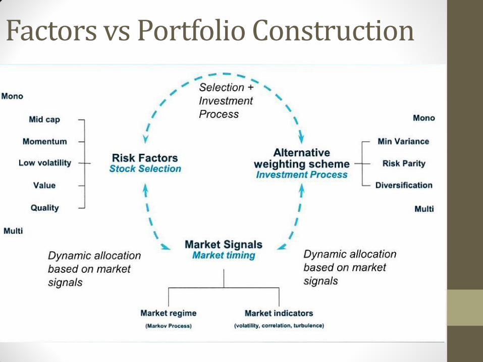
Factors vs Portfolio Construction

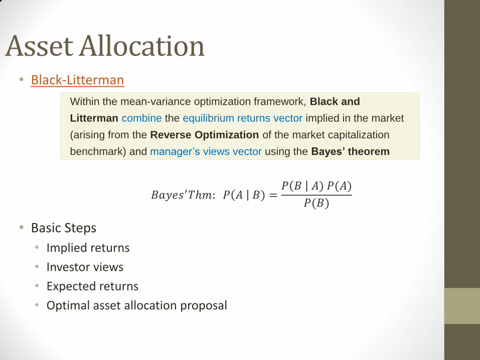
Asset Allocation • Black-Litterman

• Basic Steps

• Implied returns

• Investor views

• Expected returns

• Optimal asset allocation proposal

Within the mean-variance optimization framework, Black and

Litterman combine the equilibrium returns vector implied in the market

(arising from the Reverse Optimization of the market capitalization

benchmark) and manager’s views vector using the Bayes’ theorem

𝐵𝑎𝑦𝑒𝑠′𝑇ℎ𝑚: 𝑃 𝐴 𝐵) =𝑃 𝐵 𝐴) 𝑃(𝐴)

𝑃(𝐵)

Implied Returns + Investor Views = Expected Returns

Risk Aversion Coefficient

• δ = (E(r) – rf)/σ2

Covariance Matrix

•∑

Market capitalization weights

• wmkt

Views

•(P)

•(Q)

Uncertainty of Views

• (Ω)

Implied return vector

•Π= δ Σ wmkt

11

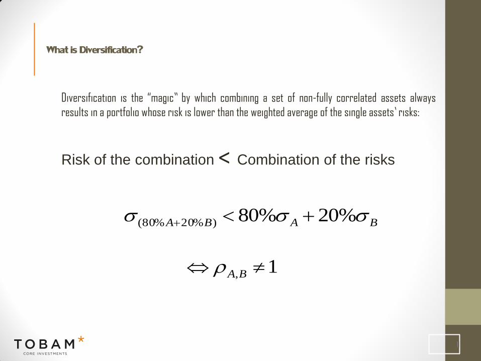
What is Diversification?

Diversification is the “magic” by which combining a set of non-fully correlated assets always

results in a portfolio whose risk is lower than the weighted average of the single assets’ risks:

Risk of the combination < Combination of the risks

1, BA

BABA %20%80)%20%80(

12

Definition of the Diversification Ratio®

TOBAM’s unique Diversification Ratio® is the tool to measure the diversification of

any portfolio P:

)(PDRThe weighted average of

stock volatilities

Portfolio Volatility

P

nnwww

...2211

X1,X2,…Xn = Risky assets in universe U

i = Volatility of asset i

P = (w1, w2,…wn) = The vector of asset weights

= (1,2,…n) = The vector of asset volatilities

V = Covariance matrix

C = Correlation matrix

Combination of Risks

Risk of the Combination

13

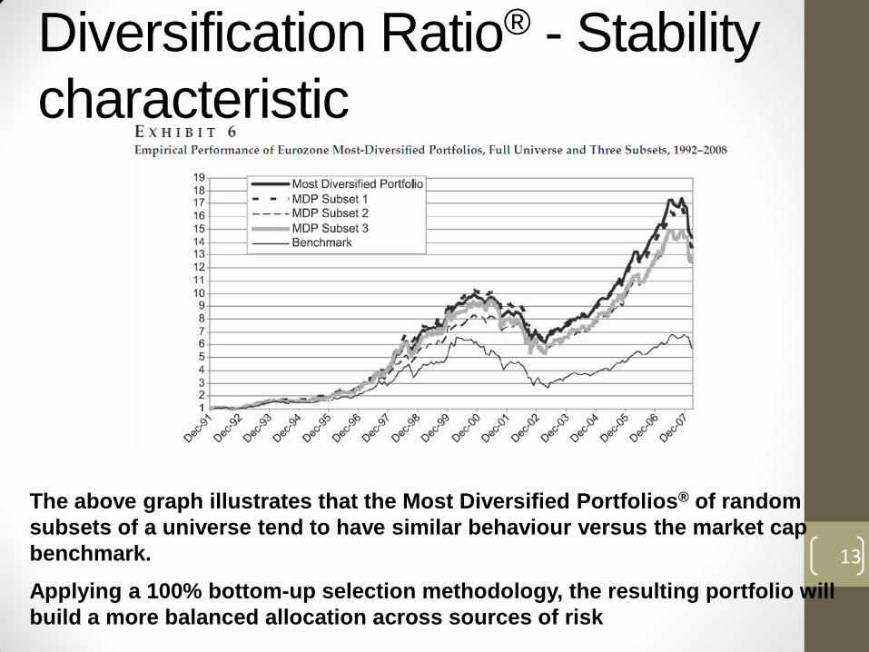
Diversification Ratio® - Stability

characteristic

The above graph illustrates that the Most Diversified Portfolios® of random

subsets of a universe tend to have similar behaviour versus the market cap

benchmark.

Applying a 100% bottom-up selection methodology, the resulting portfolio will

build a more balanced allocation across sources of risk

Growth Model

• US Cycle Model: (Goldman Sachs). • Objetivo: usar variables macroeconómicas para entender el estado del

ciclo económico Norteamericano.

• Principio: La economía Norteamericana esta en ciclo positivo cuando: -Múltiplos suben

-Empresas suben utilidades (EPS, ROE)

-Momentum positivo de producción (ISM Manufacturero)

-Tasas suben y curva se empina

-Dólar sube.

• Variables (+1 si >0, -1 si <0): • Russell 3000 P/E FRW, variación 1Y

• Russell 3000 Trail 12M EPS , variación 1Y

• S&P 500 ROE, variación 1Y

• 10y Treasury , variación 1M, 6M, 12M

• 10y-2y US Slope, nivel vs promedio 10Y

• DXY (Dollar Index), variación 1M, 6M, 12M

• ISM Man., variación 1M, 6M, 12M

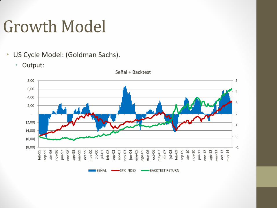
Growth Model

• US Cycle Model: (Goldman Sachs).

• Output:

-1

0

1

2

3

4

5

(8,00)

(6,00)

(4,00)

(2,00)

-

2,00

4,00

6,00

8,00

feb

-95

sep

-95

abr-

96

no

v-9

6

jun

-97

ene

-98

ago

-98

mar

-99

oct

-99

may

-00

dic

-00

jul-

01

feb

-02

sep

-02

abr-

03

no

v-0

3

jun

-04

ene

-05

ago

-05

mar

-06

oct

-06

may

-07

dic

-07

jul-

08

feb

-09

sep

-09

abr-

10

no

v-1

0

jun

-11

ene

-12

ago

-12

mar

-13

oct

-13

may

-14

Señal + Backtest

SEÑAL SPX INDEX BACKTEST RETURN

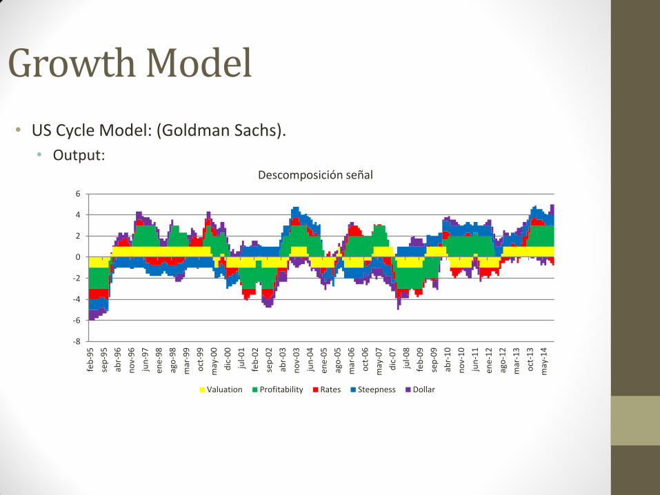
Growth Model

• US Cycle Model: (Goldman Sachs).

• Output:

-8

-6

-4

-2

0

2

4

6

feb

-95

sep

-95

abr-

96

no

v-9

6

jun

-97

ene

-98

ago

-98

mar

-99

oct

-99

may

-00

dic

-00

jul-

01

feb

-02

sep

-02

abr-

03

no

v-0

3

jun

-04

ene

-05

ago

-05

mar

-06

oct

-06

may

-07

dic

-07

jul-

08

feb

-09

sep

-09

abr-

10

no

v-1

0

jun

-11

ene

-12

ago

-12

mar

-13

oct

-13

may

-14

Descomposición señal

Valuation Profitability Rates Steepness Dollar

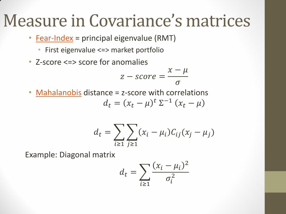
Measure in Covariance’s matrices • Fear-Index = principal eigenvalue (RMT)

• First eigenvalue <=> market portfolio

• Z-score <=> score for anomalies

𝑧 − 𝑠𝑐𝑜𝑟𝑒 =𝑥 − 𝜇

𝜎

• Mahalanobis distance = z-score with correlations 𝑑𝑡 = 𝑥𝑡 − 𝜇

𝑡 Σ−1 𝑥𝑡 − 𝜇

𝑑𝑡 = 𝑥𝑖 − 𝜇𝑖 𝐶𝑖𝑗(𝑥𝑗 − 𝜇𝑗)

𝑗≥1𝑖≥1

Example: Diagonal matrix

𝑑𝑡 = 𝑥𝑖 − 𝜇𝑖

2

𝜎𝑖2

𝑖≥1

Turbulence

Turbulence

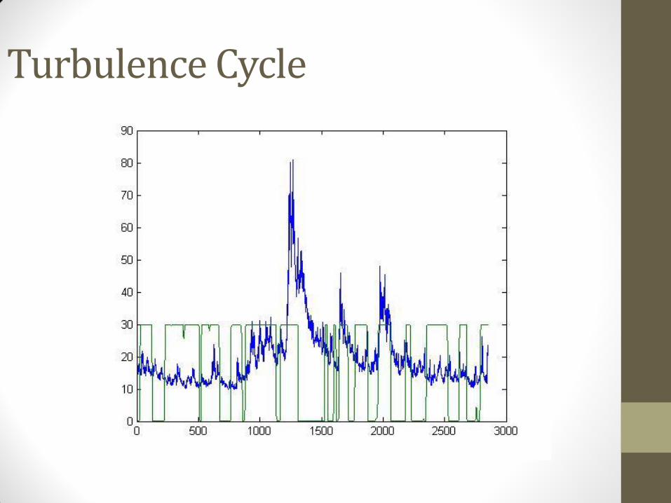
Turbulence Cycle

Backtest A-E

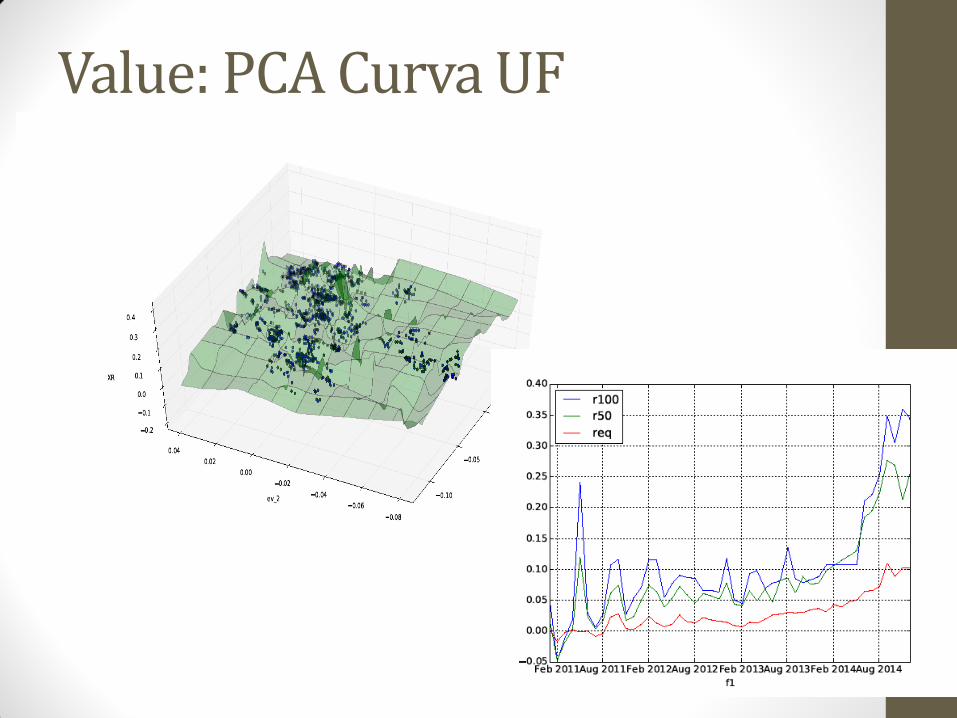
Value: PCA Curva UF

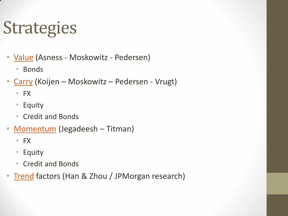
Strategies

• Value (Asness - Moskowitz - Pedersen)

• Bonds

• Carry (Koijen – Moskowitz – Pedersen - Vrugt)

• FX

• Equity

• Credit and Bonds

• Momentum (Jegadeesh – Titman)

• FX

• Equity

• Credit and Bonds

• Trend factors (Han & Zhou / JPMorgan research)

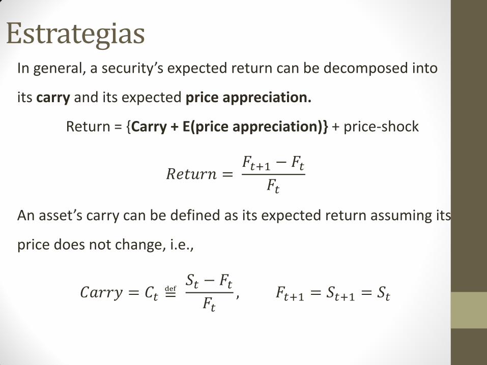
Estrategias In general, a security’s expected return can be decomposed into

its carry and its expected price appreciation.

Return = Carry + E(price appreciation) + price-shock

𝑅𝑒𝑡𝑢𝑟𝑛 = 𝐹𝑡+1 − 𝐹𝑡𝐹𝑡

An asset’s carry can be defined as its expected return assuming its

price does not change, i.e.,

𝐶𝑎𝑟𝑟𝑦 = 𝐶𝑡 ≝ 𝑆𝑡 − 𝐹𝑡𝐹𝑡, 𝐹𝑡+1 = 𝑆𝑡+1 = 𝑆𝑡

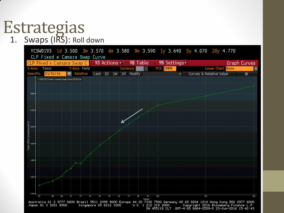
Estrategias 1. Swaps (IRS): Roll down

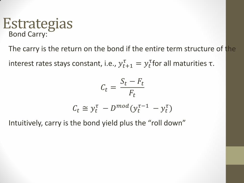
Estrategias Bond Carry:

The carry is the return on the bond if the entire term structure of the

interest rates stays constant, i.e., 𝑦𝑡+1𝜏 = 𝑦𝑡

τfor all maturities τ.

𝐶𝑡 = 𝑆𝑡 − 𝐹𝑡𝐹𝑡

𝐶𝑡 ≅ 𝑦𝑡𝜏 − 𝐷𝑚𝑜𝑑(𝑦𝑡

𝜏−1 − 𝑦𝑡𝜏)

Intuitively, carry is the bond yield plus the “roll down”

Estrategias Equity Carry:

In Equity, carry represents the expected dividend yield. If stock prices

do not change, then the return on equity comes from dividends.

𝐹𝑡 = 𝑆𝑡 1 + 𝑟𝑓 − Et(Dt+1)

𝐶𝑡 = 𝑆𝑡 − 𝐹𝑡𝐹𝑡

𝐶𝑡 =𝐸𝑡 𝐷𝑡𝑆𝑡− 𝑟𝑓

𝑆𝑡𝐹𝑡

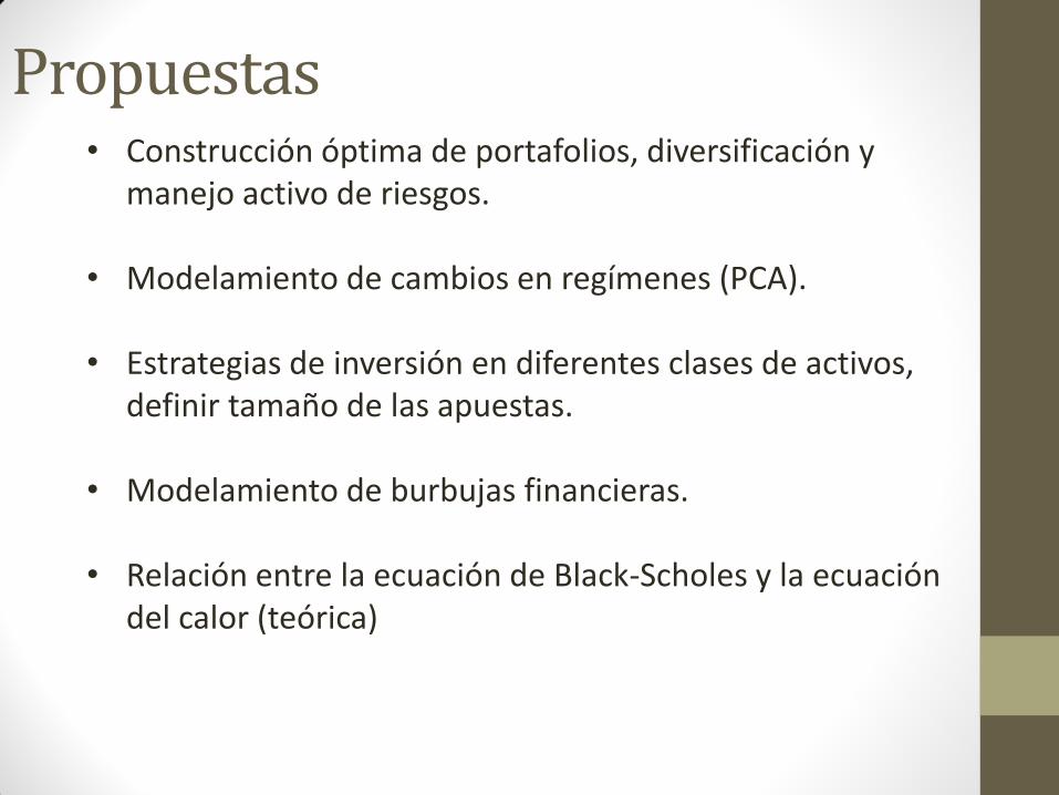
Propuestas • Construcción óptima de portafolios, diversificación y

manejo activo de riesgos.

• Modelamiento de cambios en regímenes (PCA).

• Estrategias de inversión en diferentes clases de activos, definir tamaño de las apuestas.

• Modelamiento de burbujas financieras.

• Relación entre la ecuación de Black-Scholes y la ecuación del calor (teórica)