determinaciÓn de los gradientes tÉrmicos … · un modelo basado en dinámica de fluidos...

233

DETERMINACIÓN DE LOS GRADIENTES TÉRMICOS NOCTURNOS EN UN INVERNADERO USANDO DINÁMICA DE FLUIDOS COMPUTACIONAL

DETERMINATION OF NIGHT-TIME THERMAL GRADIENTS IN A GREENHOUSE USING COMPUTATIONAL THERMAL DYNAMICS

Verónica Espinal-Montes*, I. Lorenzo López-Cruz, Abraham Rojano-Aguilar, Eugenio Romantchik-Kriuchova, Armando Ramírez-Arias

Posgrado en Ingeniería Agrícola y Uso Integral del Agua, Universidad Autónoma Chapingo. 56230. Chapingo, Estado de México. ([email protected]).

Resumen

En regiones con climas secos y templados, como los del centro y norte de México, los productores de cultivos en invernadero enfrentan temperaturas nocturnas bajas, que se agudizan en algunas temporadas del año. En un invernadero éstas pueden contrarrestarse con sistemas de calefacción; pero cuando no se tiene el recurso, el ingreso de aire frío se evita con el cierre de ventanas. El objetivo del presente estudio fue desarrollar un modelo basado en Dinámica de Fluidos Computacional (CFD) para evaluar las variaciones de temperatura y flujo de aire nocturno en un invernadero en dos escenarios: ventanas laterales cerradas y abiertas. Los datos usados en las simula-ciones fueron recolectados durante el invierno de 2012, en un invernadero tipo sierra con cubierta de polietileno y un área de 1 834.65 m2, localizado en la unidad agrícola experi-mental de la Universidad Autónoma Chapingo. Las simula-ciones se realizaron con el programa comercial CFD ANSYS-Fluent y un modelo 3D. Para establecer las condiciones de frontera y validación del modelo, se midió la temperatura del aire, cubierta y suelo dentro del invernadero. Los resultados experimentales y las simulaciones presentaron un efecto de inversión térmica, en el cual la temperatura del invernadero fue menor que la exterior. La simulación del invernadero con ventanas cerradas mostró una inversión térmica promedio de 3.1 K y los datos experimentales de 3.3 K; con ventanas abiertas el modelo CFD predijo una inversión térmica de 0.8 K. La apertura de ventanas permitió la circulación del aire, lo cual equilibró la temperatura interior con la exterior. Los resultados mostraron la capacidad de CFD para simular con precisión el microclima del invernadero, y por lo tanto su aplicación en el diseño y manejo de invernaderos.

Palabras clave: Modelo numérico, inversión térmica, CFD.

* Autor responsable v Author for correspondence.Recibido: noviembre, 2014. Aprobado: febrero, 2015.Publicado como ARTÍCULO en Agrociencia 49: 233-247. 2015.

AbstRAct

In regions with dry and temperate climates, such as those of central and northern Mexico, the producers of greenhouse crops face low night-time temperatures, which become more severe during certain periods of the year. In a greenhouse they can be counteracted with heating systems, but when this resource is not available, the entrance of cold air is avoided by closing windows. The objective of the present study was to develop a model based on Computational Fluid Dynamics (CFD) in order to evaluate the variations of night-time temperature and air flow in a greenhouse in two scenarios: lateral windows open and closed. The data used in the simulations were collected during the winter of 2012, in a sierra type greenhouse with polyethylene cover and an area of 1 834.65 m2, located at the experimental agricultural unit of the Universidad Autónoma Chapingo. The simulations were made with the commercial program CFD ANSYS-Fluent and a 3D model. To establish the conditions of boundary and validation of the model, temperature of air, cover and soil was measured inside the greenhouse. The experimental results and simulations presented an effect of thermal inversion, in which the temperature of the greenhouse was lower than the exterior. The simulation of the greenhouse with closed windows showed an average thermal inversion of 3.1 K and the experimental data of 3.3 K; with open windows the CFD model predicted a thermal inversion of 0.8 K. The opening of windows allowed air circulation, which balanced the inside temperature with the exterior. Results showed the capacity of the CFD to simulate the microclimate of the greenhouse with precision, and therefore its application in the design and management of greenhouses.

Key words: Numerical model, thermal inversion, CFD.

AGROCIENCIA, 1 de abril - 15 de mayo, 2015

VOLUMEN 49, NÚMERO 3234

IntRoduccIón

Los invernaderos mexicanos mayores a una hectárea, generalmente tienen los sistemas necesarios para el control del microclima. En

contraste, los invernaderos menores solo cuentan con la estructura cubierta por polietileno. Un invernade-ro mal diseñado puede presentar un microclima con temperaturas extremas, niveles de humedad que pue-den afectar al cultivo y deficiencia de CO2, debido a la circulación inadecuada del aire. Un problema cli-mático principal en el centro y norte de México son las temperaturas nocturnas bajas durante el invierno. En un invernadero, éstas pueden contrarrestarse con sistemas de calefacción, pero si no es posible, una práctica común es el cierre de ventanas para evitar el ingreso del aire frío.

Algunos métodos usados para estudiar el micro-clima de invernaderos son los modelos analíticos, empíricos, experimentales en escala pequeña, expe-rimentales a escala completa, de redes multizonales, zonales y modelos de CFD (Chen, 2009). CFD es una rama de la mecánica de fluidos que usa algorit-mos y métodos numéricos para resolver problemas que involucran flujos, y se aplica para modelar el mi-croclima de invernaderos. La mayoría de los estudios describen los campos de flujo y temperatura dentro del invernadero, con el cálculo de tasas de intercam-bio de aire y optimizando tamaño y localización de ventanas (Romero-Gómez et al., 2010).

En la literatura revisada hay pocos estudios acerca del análisis del clima nocturno en invernaderos me-diante CFD. Montero et al. (2005) desarrollaron un modelo CFD 2D para analizar un invernadero sin calefacción, comparando con el efecto de agregar una cortina interna de polietileno horizontal, y encontra-ron que en noches despejadas (cuando la temperatura del cielo es menor que la exterior, dependiendo si el ambiente presenta baja o alta humedad) el inverna-dero sin cortina presentó una inversión térmica de 2.5 K, que en el techo alcanzó hasta 4.4 K. En noches completamente nubladas, cuando se considera que la temperatura del cielo es igual a la exterior, la tem-peratura del aire en el interior fue 3.6 K mayor que la exterior. El uso de la cortina permitió mantener la temperatura del aire del invernadero superior a la del exterior, en noches despejadas y nubladas. Igle-sias et al. (2009) compararon el mismo invernadero, usando cubierta sencilla y doble; en noches despejadas

IntRoductIon

Mexican greenhouses larger than one hectare generally have the systems necessary for the control of the microclimate. In contrast,

smaller greenhouses have only the polyethylene cover on the structure. A poorly designed greenhouse can have a microclimate with extreme temperatures, moisture levels that can affect the crop and deficiency of CO2, due to the inadequate circulation of air. One of the principal climatic problems in central and northern Mexico is low night-time temperatures, during the winter. In a greenhouse, this can be counteracted with a heating system, but if not possible, a common practice is to close the windows to avoid the entrance of cold air.

Some methods used to study the microclimate of a greenhouse are the analytical, empirical and experimental models on a small scale, full scale experimental models, of multi-zonal and zonal networks and CFD models (Chen, 2009). CFD is a branch of the mechanics of fluids that uses algorithms and numerical methods for solving problems that involve flows, and it is applied for modeling the microclimate of greenhouses. Most of these studies describe the temperature and flow fields inside the greenhouse, with the calculation of exchange rates of air and optimizing size and location of windows (Romero-Gómez et al., 2010).

In the literature reviewed there are few studies about the analysis of night-time climate in greenhouses using CFD. Montero et al. (2005) developed a 2D CFD model to analyze a greenhouse without heating, comparing with the effect of adding an internal curtain of horizontal polyethylene, and found that on clear nights (when the temperature of the ceiling is lower than the exterior depending if the environment shows low or high humidity), the greenhouse without the curtain presented a thermal inversion of 2.5 K, which on the roof reached 4.4 K. On completely cloudy nights, in which it is considered that the temperature of the ceiling is equal to the exterior, the air temperature in the interior was 3.6 K higher than the exterior. The use of the curtain made it possible to maintain the air temperature of the greenhouse higher than that of the exterior, on both clear and cloudy nights. Iglesias et al. (2009) compared the same greenhouse, using simple and double cover; on clear nights they obtained a thermal

235ESPI NAL-MONTES et al.


obtuvieron una inversión térmica de 2.5 K con la cu-bierta sencilla, y con la cubierta doble la diferencia fue 0.5 K sobre la temperatura exterior.

Montero et al. (2013) usaron un modelo 2D para evaluar un invernadero en tres condiciones: sin cale-facción, con una cortina externa y con una cortina interna, para noches despejadas y completamente nubladas. En el primer caso la inversión térmica pro-medio fue 2.5 K. La cortina externa evitó la inversión térmica en noches despejadas y nubladas, igual que la cortina interna, aunque para el caso despejado, pre-sentó inversión térmica en el aire por encima de la cortina, y fue cercana a 3.5 K.

El objetivo de esta investigación fue generar un modelo CFD 3D para un invernadero del centro de México, que permita predecir el comportamiento de la temperatura y el flujo de aire nocturnos al consi-derar la apertura y el cierre de las ventanas laterales; además, evaluar el ajuste del modelo CFD en la pre-dicción de las temperaturas.

mAteRIAles y métodos

Características del invernadero y mediciones

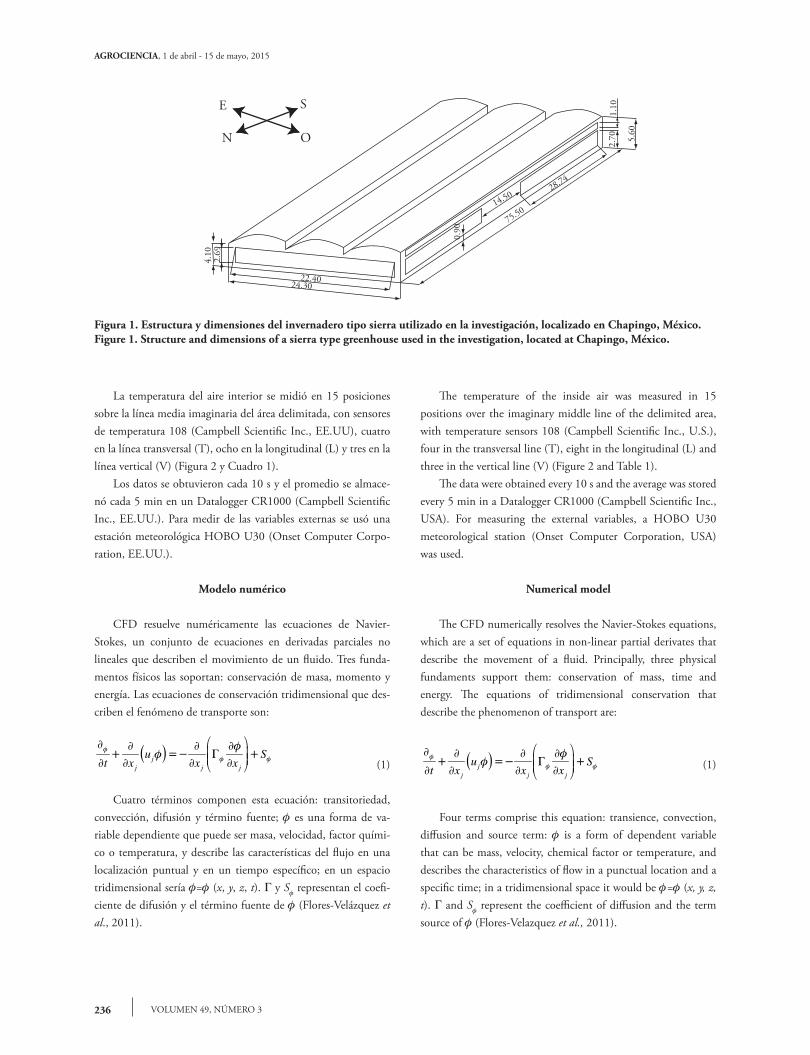
La fase experimental se realizó en un invernadero tipo sierra de tres naves (Figura 1) localizado en la Universidad Autónoma Chapingo, México (19° 29’ N, 98° 53’ O y 2250 m de altitud).

Las características del invernadero son: largo 75.5 m, ancho 24.3 m, altura máxima 6.45 m, orientación SE-NO y volumen 10 838 m3. El área total de ventanas laterales y cenitales es 668.89 m2, las ventanas cenitales están orientadas hacia el oeste. Tiene cubierta de polietileno de una sola capa y malla anti-trips de 52 x 26 hilos en las ventanas. Las mediciones se realizaron solo en una sexta parte del invernadero, por lo cual el área de estudio se delimitó con paredes de polietileno.

Para establecer las condiciones de frontera y validar el mo-delo CFD, la temperatura se midió en el aire, suelo y cubierta en el interior del invernadero, y en el aire en el exterior. Las me-diciones se realizaron durante las noches del invierno del 2012 de las 19:00 h a 6:00 h. La humedad relativa se midió en el cen-tro de la zona de estudio a una altura de 2.07 m con un sensor HMP50 (Campbell Scientific Inc., EE.UU.). La velocidad del viento se midió con un anemómetro sónico WindSonic4 (Gill Instruments, EE.UU.) ubicado en el centro, a 2.80 m de altu-ra. La temperatura de la cubierta se midió con dos termopares FW3 (Campbell Scientific Inc., EE.UU.) y la del suelo con dos sensores de temperatura 107 (Campbell Scientific Inc., EE.UU.) enterrados en el suelo, al centro del invernadero, a 5 cm de pro-fundidad.

inversion of 2.5 K with the simple cover, and with the double cover the difference was 0.5 K above the external temperature.

Montero et al. (2013) used a 2D model to evaluate a greenhouse under three conditions: unheated, with an external curtain and with an interior curtain, for clear and completely cloudy nights. In the first case the average thermal inversion was 2.5 K. The external curtain prevented thermal inversion on clear and cloudy nights, as did the interior curtain, although for the case of clear nights, there was thermal inversion in the air above the curtain of approximately 3.5 K. The objective of the present study was to generate a 3D CFD model for a greenhouse of central Mexico, which allows the prediction of the behavior of night-time temperature and air flow considering the opening and closing of the lateral windows, as well as to evaluate the adjustment of the CFD model in the prediction of temperatures.

mAteRIAls And methods

Characteristics of the greenhouse and measurements

The experimental phase was carried out in a sierra type greenhouse of three naves (Figure 1) located at the Universidad Autónoma Chapingo, Mexico (19° 29’ N, 98° 53’ W and 2250 m altitude).

The characteristics of the greenhouse are as follows: length 75.5 m, width 24.3 m, maximum height 6.45 m, orientation SE-NW and volume 10 838 m3. Total area of lateral and zenithal windows is 668.89 m2; the zenithal windows are oriented to the west. It has a polyethylene cover of a single layer and anti-trips screen of 52 x 26 threads in the windows. The measurements were made only in the sixth part of the greenhouse, thus the area of study was delimited with polyethylene walls.

To establish the conditions of boundary and validate the CFD model, temperature was measured in the air, soil and the cover, in the interior of the greenhouse, and that of the air in the exterior. The measurements were made during the winter nights of 2012 from 19:00 h to 6:00 h. Relative humidity was measured in the center of the study zone at a height of 2.07 m with an HMP50 sensor (Campbell Scientific Inc., USA). Wind speed was measured with a WindSonic4 sonic anemometer (Gill Instruments, USA) located in the center, at 2.80 m height. The temperature of the cover was measured with two FW3 thermocouples (Campbell Scientific Inc., USA) and that of the soil using two temperature sensons 107 (Campbell Scientific Inc., USA) buried in the soil, at the center of the greenhouse, at a depth of 5 cm.



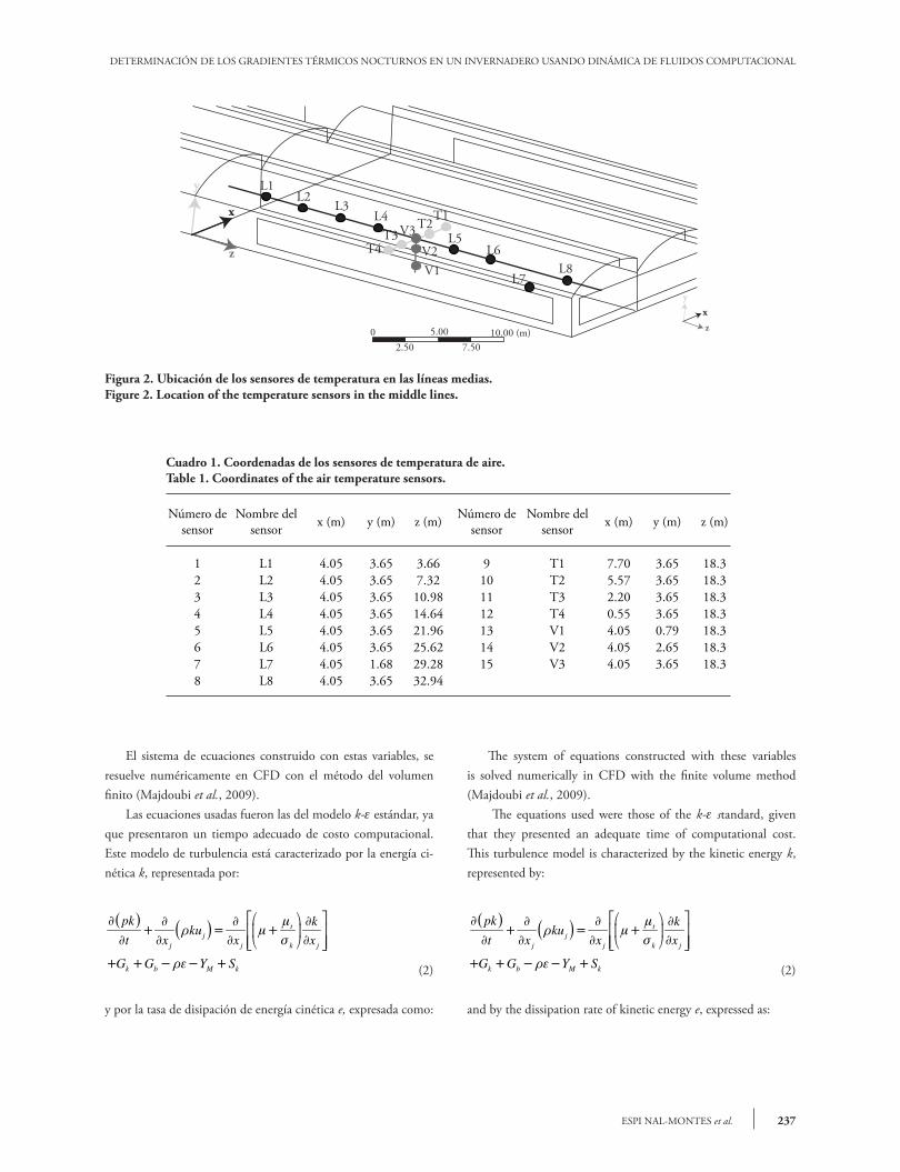
La temperatura del aire interior se midió en 15 posiciones sobre la línea media imaginaria del área delimitada, con sensores de temperatura 108 (Campbell Scientific Inc., EE.UU), cuatro en la línea transversal (T), ocho en la longitudinal (L) y tres en la línea vertical (V) (Figura 2 y Cuadro 1).

Los datos se obtuvieron cada 10 s y el promedio se almace-nó cada 5 min en un Datalogger CR1000 (Campbell Scientific Inc., EE.UU.). Para medir de las variables externas se usó una estación meteorológica HOBO U30 (Onset Computer Corpo-ration, EE.UU.).

Modelo numérico

CFD resuelve numéricamente las ecuaciones de Navier-Stokes, un conjunto de ecuaciones en derivadas parciales no lineales que describen el movimiento de un fluido. Tres funda-mentos físicos las soportan: conservación de masa, momento y energía. Las ecuaciones de conservación tridimensional que des-criben el fenómeno de transporte son:

jj j j

u St x x xf

f f

f f - G (1)

Cuatro términos componen esta ecuación: transitoriedad, convección, difusión y término fuente; f es una forma de va-riable dependiente que puede ser masa, velocidad, factor quími-co o temperatura, y describe las características del flujo en una localización puntual y en un tiempo específico; en un espacio tridimensional sería f=f (x, y, z, t). G y S

f representan el coefi-

ciente de difusión y el término fuente de f (Flores-Velázquez et al., 2011).

The temperature of the inside air was measured in 15 positions over the imaginary middle line of the delimited area, with temperature sensors 108 (Campbell Scientific Inc., U.S.), four in the transversal line (T), eight in the longitudinal (L) and three in the vertical line (V) (Figure 2 and Table 1).

The data were obtained every 10 s and the average was stored every 5 min in a Datalogger CR1000 (Campbell Scientific Inc., USA). For measuring the external variables, a HOBO U30 meteorological station (Onset Computer Corporation, USA) was used.

Numerical model

The CFD numerically resolves the Navier-Stokes equations, which are a set of equations in non-linear partial derivates that describe the movement of a fluid. Principally, three physical fundaments support them: conservation of mass, time and energy. The equations of tridimensional conservation that describe the phenomenon of transport are:

jj j j

u St x x xf

f f

f f - G (1)

Four terms comprise this equation: transience, convection, diffusion and source term: f is a form of dependent variable that can be mass, velocity, chemical factor or temperature, and describes the characteristics of flow in a punctual location and a specific time; in a tridimensional space it would be f=f (x, y, z, t). G and S

f represent the coefficient of diffusion and the term

source of f (Flores-Velazquez et al., 2011).

Figura 1. Estructura y dimensiones del invernadero tipo sierra utilizado en la investigación, localizado en Chapingo, México.Figure 1. Structure and dimensions of a sierra type greenhouse used in the investigation, located at Chapingo, México.

22.40

4.10

2.69

5.60

14.50

24.30

0.90

75.50

28.74

1.10

2.70N

SE

O



El sistema de ecuaciones construido con estas variables, se resuelve numéricamente en CFD con el método del volumen finito (Majdoubi et al., 2009).

Las ecuaciones usadas fueron las del modelo k-e estándar, ya que presentaron un tiempo adecuado de costo computacional. Este modelo de turbulencia está caracterizado por la energía ci-nética k, representada por:

tj

j j k j

k b M k

pk kku

t x x x

G G Y S

m m

s

- e- (2)

y por la tasa de disipación de energía cinética e, expresada como:

Figura 2. Ubicación de los sensores de temperatura en las líneas medias.Figure 2. Location of the temperature sensors in the middle lines.

Cuadro 1. Coordenadas de los sensores de temperatura de aire.Table 1. Coordinates of the air temperature sensors.

Número de sensor

Nombre del sensor x (m) y (m) z (m) Número de

sensorNombre del

sensor x (m) y (m) z (m)

1 L1 4.05 3.65 3.66 9 T1 7.70 3.65 18.32 L2 4.05 3.65 7.32 10 T2 5.57 3.65 18.33 L3 4.05 3.65 10.98 11 T3 2.20 3.65 18.34 L4 4.05 3.65 14.64 12 T4 0.55 3.65 18.35 L5 4.05 3.65 21.96 13 V1 4.05 0.79 18.36 L6 4.05 3.65 25.62 14 V2 4.05 2.65 18.37 L7 4.05 1.68 29.28 15 V3 4.05 3.65 18.38 L8 4.05 3.65 32.94

x

z

y L1L2

L3L4

L5L6

L7L8

T1T2T3

T4

V1V2

V3

0 5.00 10.00 (m)2.50 7.50

yx

z

The system of equations constructed with these variables is solved numerically in CFD with the finite volume method (Majdoubi et al., 2009). The equations used were those of the k-e standard, given that they presented an adequate time of computational cost. This turbulence model is characterized by the kinetic energy k, represented by:

tj

j j k j

k b M k

pk kku

t x x x

G G Y S

m m

s

- e- (2)

and by the dissipation rate of kinetic energy e, expressed as:



2

1 3 2

tj

j j j

k b

ut x x x

C G C G C Sk k

e

e e e

e m e e m

s

e e - e

(3)

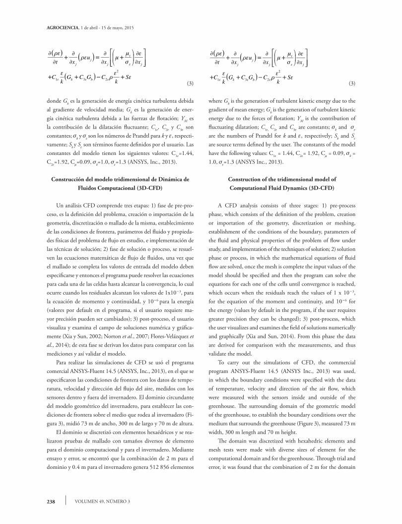
donde Gk es la generación de energía cinética turbulenta debida al gradiente de velocidad media; Gb es la generación de ener-gía cinética turbulenta debida a las fuerzas de flotación; YM es la contribución de la dilatación fluctuante; C1e, C2e y C3e son constantes; sk y s

e son los números de Prandtl para k y e, respecti-vamente; Sk y S

e son términos fuente definidos por el usuario. Las

constantes del modelo tienen los siguientes valores: C1e=1.44, C2e=1.92, C

m=0.09, sk=1.0, s

e=1.3 (ANSYS, Inc., 2013).

Construcción del modelo tridimensional de Dinámica de Fluidos Computacional (3D-CFD)

Un análisis CFD comprende tres etapas: 1) fase de pre-pro-ceso, es la definición del problema, creación o importación de la geometría, discretización o mallado de la misma, establecimiento de las condiciones de frontera, parámetros del fluido y propieda-des físicas del problema de flujo en estudio, e implementación de las técnicas de solución; 2) fase de solución o proceso, se resuel-ven las ecuaciones matemáticas de flujo de fluidos, una vez que el mallado se completa los valores de entrada del modelo deben especificarse y entonces el programa puede resolver las ecuaciones para cada una de las celdas hasta alcanzar la convergencia, lo cual ocurre cuando los residuales alcanzan los valores de 1x10-3, para la ecuación de momento y continuidad, y 10-6 para la energía (valores por default en el programa, si el usuario requiere ma-yor precisión pueden ser cambiados); 3) post-proceso, el usuario visualiza y examina el campo de soluciones numérica y gráfica-mente (Xia y Sun, 2002; Norton et al., 2007; Flores-Velázquez et al., 2014); de esta fase se derivan los datos para comparar con las mediciones y así validar el modelo.

Para realizar las simulaciones de CFD se usó el programa comercial ANSYS-Fluent 14.5 (ANSYS, Inc., 2013), en el que se especificaron las condiciones de frontera con los datos de tempe-ratura, velocidad y dirección del flujo del aire, medidos con los sensores dentro y fuera del invernadero. El dominio circundante del modelo geométrico del invernadero, para establecer las con-diciones de frontera sobre el medio que rodea al invernadero (Fi-gura 3), midió 73 m de ancho, 300 m de largo y 70 m de altura.

El dominio se discretizó con elementos hexaédricos y se rea-lizaron pruebas de mallado con tamaños diversos de elemento para el dominio computacional y para el invernadero. Mediante ensayo y error, se encontró que la combinación de 2 m para el dominio y 0.4 m para el invernadero genera 512 856 elementos

2

1 3 2

tj

j j j

k b

ut x x x

C G C G C Sk k

e

e e e

e m e e m

s

e e - e

(3)

where Gk is the generation of turbulent kinetic energy due to the gradient of mean energy; Gb is the generation of turbulent kinetic energy due to the forces of flotation; YM is the contribution of fluctuating dilatation; C1e, C2e and C3e are constants; sk and s

e

are the numbers of Prandtl for k and e, respectively; Sk and Se

are source terms defined by the user. The constants of the model have the following values: C1e = 1.44, C2e= 1.92, C

m = 0.09, sk =

1.0, se=1.3 (ANSYS Inc., 2013).

Construction of the tridimensional model of Computational Fluid Dynamics (3D-CFD)

A CFD analysis consists of three stages: 1) pre-process phase, which consists of the definition of the problem, creation or importation of the geometry, discretization or meshing, establishment of the conditions of the boundary, parameters of the fluid and physical properties of the problem of flow under study, and implementation of the techniques of solution; 2) solution phase or process, in which the mathematical equations of fluid flow are solved, once the mesh is complete the input values of the model should be specified and then the program can solve the equations for each one of the cells until convergence is reached, which occurs when the residuals reach the values of 1 x 10-3, for the equation of the moment and continuity, and 10-6 for the energy (values by default in the program, if the user requires greater precision they can be changed); 3) post-process, which the user visualizes and examines the field of solutions numerically and graphically (Xia and Sun, 2014). From this phase the data are derived for comparison with the measurements, and thus validate the model.

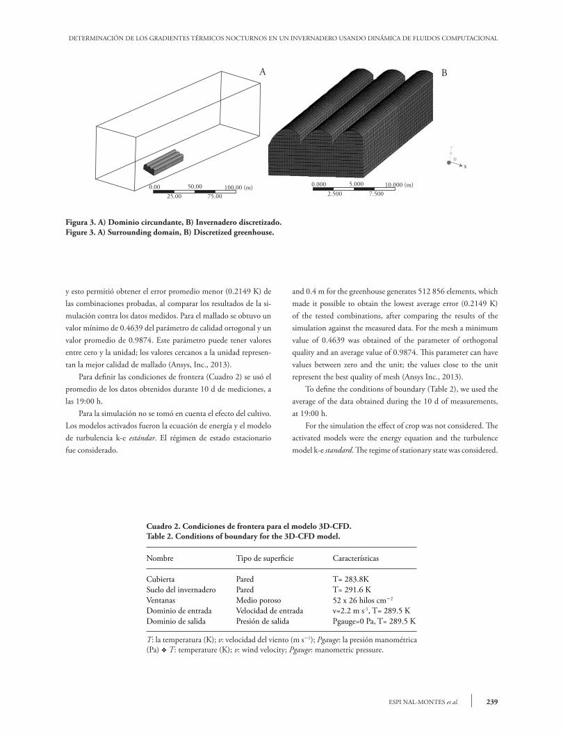
To carry out the simulations of CFD, the commercial program ANSYS-Fluent 14.5 (ANSYS Inc., 2013) was used, in which the boundary conditions were specified with the data of temperature, velocity and direction of the air flow, which were measured with the sensors inside and outside of the greenhouse. The surrounding domain of the geometric model of the greenhouse, to establish the boundary conditions over the medium that surrounds the greenhouse (Figure 3), measured 73 m width, 300 m length and 70 m height.

The domain was discretized with hexahedric elements and mesh tests were made with diverse sizes of element for the computational domain and for the greenhouse. Through trial and error, it was found that the combination of 2 m for the domain



y esto permitió obtener el error promedio menor (0.2149 K) de las combinaciones probadas, al comparar los resultados de la si-mulación contra los datos medidos. Para el mallado se obtuvo un valor mínimo de 0.4639 del parámetro de calidad ortogonal y un valor promedio de 0.9874. Este parámetro puede tener valores entre cero y la unidad; los valores cercanos a la unidad represen-tan la mejor calidad de mallado (Ansys, Inc., 2013).

Para definir las condiciones de frontera (Cuadro 2) se usó el promedio de los datos obtenidos durante 10 d de mediciones, a las 19:00 h.

Para la simulación no se tomó en cuenta el efecto del cultivo. Los modelos activados fueron la ecuación de energía y el modelo de turbulencia k-e estándar. El régimen de estado estacionario fue considerado.

Figura 3. A) Dominio circundante, B) Invernadero discretizado.Figure 3. A) Surrounding domain, B) Discretized greenhouse.

Cuadro 2. Condiciones de frontera para el modelo 3D-CFD.Table 2. Conditions of boundary for the 3D-CFD model.

Nombre Tipo de superficie Características

Cubierta Pared T= 283.8KSuelo del invernadero Pared T= 291.6 KVentanas Medio poroso 52 x 26 hilos cm-2

Dominio de entrada Velocidad de entrada v=2.2 m s-1, T= 289.5 KDominio de salida Presión de salida Pgauge=0 Pa, T= 289.5 K

T: la temperatura (K); v: velocidad del viento (m s-1); Pgauge: la presión manométrica (Pa) v T: temperature (K); v: wind velocity; Pgauge: manometric pressure.

0.00 50.00 100.00 (m)25.00 75.00

0.000 5.000 10.000 (m)2.500 7.500

y

x

A B

and 0.4 m for the greenhouse generates 512 856 elements, which made it possible to obtain the lowest average error (0.2149 K) of the tested combinations, after comparing the results of the simulation against the measured data. For the mesh a minimum value of 0.4639 was obtained of the parameter of orthogonal quality and an average value of 0.9874. This parameter can have values between zero and the unit; the values close to the unit represent the best quality of mesh (Ansys Inc., 2013).

To define the conditions of boundary (Table 2), we used the average of the data obtained during the 10 d of measurements, at 19:00 h.

For the simulation the effect of crop was not considered. The activated models were the energy equation and the turbulence model k-e standard. The regime of stationary state was considered.



ResultAdos y dIscusIón

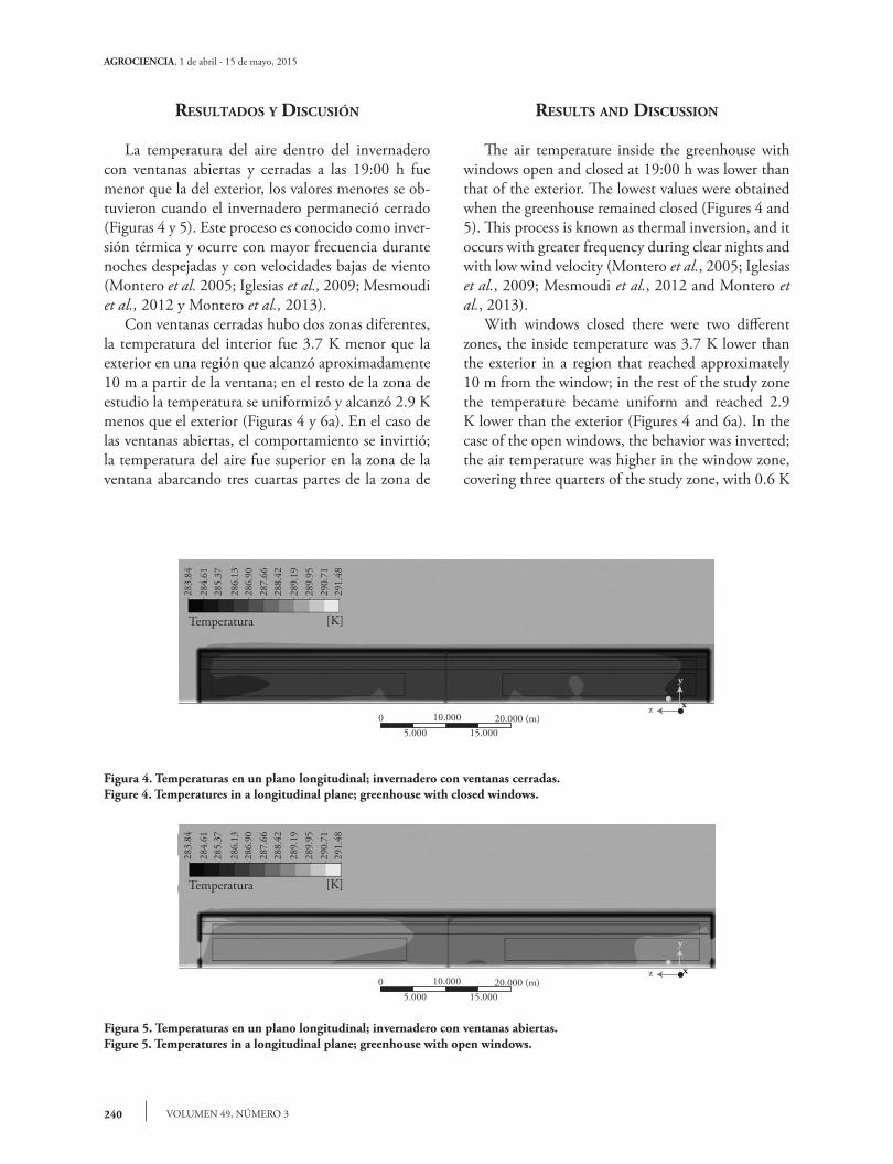
La temperatura del aire dentro del invernadero con ventanas abiertas y cerradas a las 19:00 h fue menor que la del exterior, los valores menores se ob-tuvieron cuando el invernadero permaneció cerrado (Figuras 4 y 5). Este proceso es conocido como inver-sión térmica y ocurre con mayor frecuencia durante noches despejadas y con velocidades bajas de viento (Montero et al. 2005; Iglesias et al., 2009; Mesmoudi et al., 2012 y Montero et al., 2013).

Con ventanas cerradas hubo dos zonas diferentes, la temperatura del interior fue 3.7 K menor que la exterior en una región que alcanzó aproximadamente 10 m a partir de la ventana; en el resto de la zona de estudio la temperatura se uniformizó y alcanzó 2.9 K menos que el exterior (Figuras 4 y 6a). En el caso de las ventanas abiertas, el comportamiento se invirtió; la temperatura del aire fue superior en la zona de la ventana abarcando tres cuartas partes de la zona de

Figura 4. Temperaturas en un plano longitudinal; invernadero con ventanas cerradas.Figure 4. Temperatures in a longitudinal plane; greenhouse with closed windows.

Figura 5. Temperaturas en un plano longitudinal; invernadero con ventanas abiertas.Figure 5. Temperatures in a longitudinal plane; greenhouse with open windows.

Results And dIscussIon

The air temperature inside the greenhouse with windows open and closed at 19:00 h was lower than that of the exterior. The lowest values were obtained when the greenhouse remained closed (Figures 4 and 5). This process is known as thermal inversion, and it occurs with greater frequency during clear nights and with low wind velocity (Montero et al., 2005; Iglesias et al., 2009; Mesmoudi et al., 2012 and Montero et al., 2013).

With windows closed there were two different zones, the inside temperature was 3.7 K lower than the exterior in a region that reached approximately 10 m from the window; in the rest of the study zone the temperature became uniform and reached 2.9 K lower than the exterior (Figures 4 and 6a). In the case of the open windows, the behavior was inverted; the air temperature was higher in the window zone, covering three quarters of the study zone, with 0.6 K

283.

84

[K]

284.

6128

5.37

286.

1328

6.90

287.

6628

8.42

289.

19

289.

95

290.

7129

1.48

Temperatura

0 10.000 20.000 (m)5.000 15.000

y

z x

283.

84

[K]

284.

6128

5.37

286.

1328

6.90

287.

6628

8.42

289.

19

289.

95

290.

7129

1.48

Temperatura

0 10.000 20.000 (m)5.000 15.000

y

z x



283.

85

[K]

284.

61

285.

38

286.

1528

6.92

287.

6828

8.45

289.

2228

9.99

290.

76

291.

52

Temperatura

0 8.000 (m)

4.000

[K]Temperatura

y

z x 0 8.000 (m)

4.000

283.

8528

4.61

285.

3828

6.15

286.

9228

7.68

288.

4528

9.22

289.

99

290.

7629

1.52

y

z x

283.

84

[K]

284.

61

285.

37

286.

13

286.

9028

7.66

288.

42

289.

19

289.

95

290.

7129

1.48

Temperatura

0 10.000 (m)

5.000

y

z x

283.

84

[K]

284.

61

285.

37

286.

1328

6.90

287.

6628

8.42

289.

1928

9.95

290.

71

291.

48

Temperatura

y

z x 0 10.000 (m)

5.000

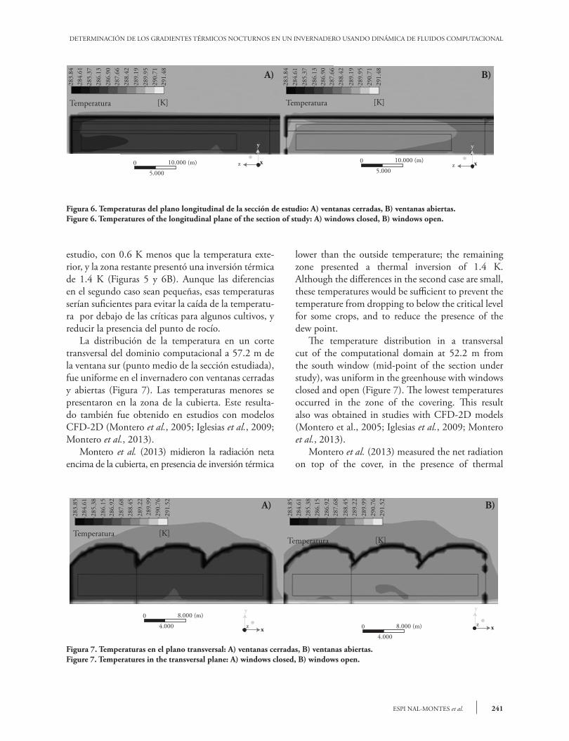
estudio, con 0.6 K menos que la temperatura exte-rior, y la zona restante presentó una inversión térmica de 1.4 K (Figuras 5 y 6B). Aunque las diferencias en el segundo caso sean pequeñas, esas temperaturas serían suficientes para evitar la caída de la temperatu-ra por debajo de las críticas para algunos cultivos, y reducir la presencia del punto de rocío.

La distribución de la temperatura en un corte transversal del dominio computacional a 57.2 m de la ventana sur (punto medio de la sección estudiada), fue uniforme en el invernadero con ventanas cerradas y abiertas (Figura 7). Las temperaturas menores se presentaron en la zona de la cubierta. Este resulta-do también fue obtenido en estudios con modelos CFD-2D (Montero et al., 2005; Iglesias et al., 2009; Montero et al., 2013).

Montero et al. (2013) midieron la radiación neta encima de la cubierta, en presencia de inversión térmica

Figura 6. Temperaturas del plano longitudinal de la sección de estudio: A) ventanas cerradas, B) ventanas abiertas.Figure 6. Temperatures of the longitudinal plane of the section of study: A) windows closed, B) windows open.

Figura 7. Temperaturas en el plano transversal: A) ventanas cerradas, B) ventanas abiertas.Figure 7. Temperatures in the transversal plane: A) windows closed, B) windows open.

lower than the outside temperature; the remaining zone presented a thermal inversion of 1.4 K. Although the differences in the second case are small, these temperatures would be sufficient to prevent the temperature from dropping to below the critical level for some crops, and to reduce the presence of the dew point.

The temperature distribution in a transversal cut of the computational domain at 52.2 m from the south window (mid-point of the section under study), was uniform in the greenhouse with windows closed and open (Figure 7). The lowest temperatures occurred in the zone of the covering. This result also was obtained in studies with CFD-2D models (Montero et al., 2005; Iglesias et al., 2009; Montero et al., 2013).

Montero et al. (2013) measured the net radiation on top of the cover, in the presence of thermal

A) B)

A) B)



durante la noche, y lo compararon con el flujo de ca-lor del suelo al aire del invernadero, el valor absoluto del primero fue mayor y se concluyó que la cubier-ta del invernadero; perdía más calor del que recibía del interior del invernadero. Según Mesmoudi et al. (2012), en condición de noches despejadas y en cal-ma, las pérdidas por radiación a través de la cubierta son altas y la temperatura de la cubierta puede caer varios grados respecto a la exterior.

CFD provee información detallada de la distribu-ción de temperaturas y campos de velocidad en cual-quier punto del dominio computacional (Montero et al., 2013). En el presente estudio los puntos de interés fueron las ubicaciones de los sensores en las líneas medias imaginarias, de los que se obtuvieron los valores de temperatura para compararlos con las mediciones realizadas.

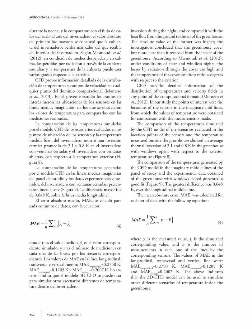
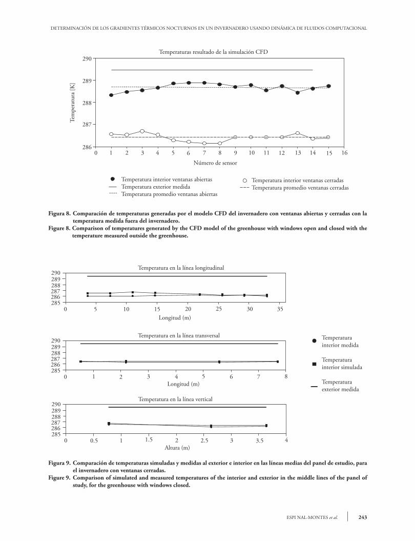
La comparación de las temperaturas simuladas por el modelo CFD de los escenarios evaluados en los puntos de ubicación de los sensores y la temperatura medida fuera del invernadero, mostró una inversión térmica promedio de 3.1 y 0.8 K en el invernadero con ventanas cerradas y el invernadero con ventanas abiertas, con respecto a la temperatura exterior (Fi-gura 8).

La comparación de las temperaturas generadas por el modelo CFD en las líneas medias imaginarias del panel de estudio y los datos experimentales obte-nidos, del invernadero con ventanas cerradas, presen-taron buen ajuste (Figura 9). La diferencia mayor fue de 0.648 K, sobre la línea media longitudinal.

El error absoluto medio, MAE, se calculó para cada conjunto de datos, con la ecuación:

-

1

1ˆ

n

i iiMAE y y

n (4)

donde yi es el valor medido, yi es el valor correspon-diente simulado, y n es el número de mediciones en cada una de las líneas por los sensores correspon-dientes. Los valores de MAE en la línea longitudinal, transversal y vertical fueron: MAElongitudinal=0.2750 K, MAEtransversal=0.1205 K y MAEvertical=0.2007 K. Lo an-terior indica que el modelo 3D-CFD se puede usar para simular otros escenarios diferentes de tempera-tura dentro del invernadero.

^

inversion during the night, and compared it with the heat flow from the ground to the air of the greenhouse. The absolute value of the former was higher; the investigators concluded that the greenhouse cover lost more heat than it received from the inside of the greenhouse. According to Mesmoudi et al. (2012), under conditions of clear and windless nights, the losses by radiation through the cover are high and the temperature of the cover can drop various degrees with respect to the exterior.

CFD provides detailed information of the distribution of temperatures and velocity fields in any point of the computational domain (Montero et al., 2013). In our study the points of interest were the locations of the sensors in the imaginary mid lines, from which the values of temperature were obtained for comparison with the measurements made.

The comparison of the temperatures simulated by the CFD model of the scenarios evaluated in the location points of the sensors and the temperature measured outside the greenhouse showed an average thermal inversion of 3.1 and 0.8 K in the greenhouse with windows open, with respect to the exterior temperature (Figure 8).

The comparison of the temperatures generated by the CFD model in the imaginary middle lines of the panel of study and the experimental data obtained of the greenhouse with windows closed presented a good fit (Figure 9). The greatest difference was 0.648 K, over the longitudinal middle line.

The mean absolute error, MAE, was calculated for each set of data with the following equation:

-

1

1ˆ

n

i iiMAE y y

n (4)

where yi is the measured value, yi is the simulated corresponding value, and n is the number of measurements in each one of the lines by the corresponding sensors. The values of MAE in the longitudinal, transversal and vertical line were: MAElongitudinal=0.2750 K, MAEtransversal=0.1205 K and MAEvertical=0.2007 K. The above indicates that the 3D-CFD model can be used to simulate other different scenarios of temperature inside the greenhouse.

^



Figura 8. Comparación de temperaturas generadas por el modelo CFD del invernadero con ventanas abiertas y cerradas con la temperatura medida fuera del invernadero.

Figure 8. Comparison of temperatures generated by the CFD model of the greenhouse with windows open and closed with the temperature measured outside the greenhouse.

Figura 9. Comparación de temperaturas simuladas y medidas al exterior e interior en las líneas medias del panel de estudio, para el invernadero con ventanas cerradas.

Figure 9. Comparison of simulated and measured temperatures of the interior and exterior in the middle lines of the panel of study, for the greenhouse with windows closed.

290

286

287

288

289

0 987654321 10 161514131211

Temperatura interior ventanas abiertasTemperatura exterior medidaTemperatura promedio ventanas abiertas

Temperatura interior ventanas cerradasTemperatura promedio ventanas cerradas

Número de sensor

Tem

pera

tura

[K

]

Temperaturas resultado de la simulación CFD

290289288287286285

0 5 10 15 20 25 30 35

Temperatura en la línea longitudinal

Longitud (m)

Temperatura interior medida

Temperatura interior simulada

Temperatura exterior medida

290289288287286285

0 1 2 3 4 5 6 7

Temperatura en la línea transversal

Longitud (m)8

290289288287286285

0 0.5 1 1.5 2 2.5 3 3.5

Temperatura en la línea vertical

Altura (m)4



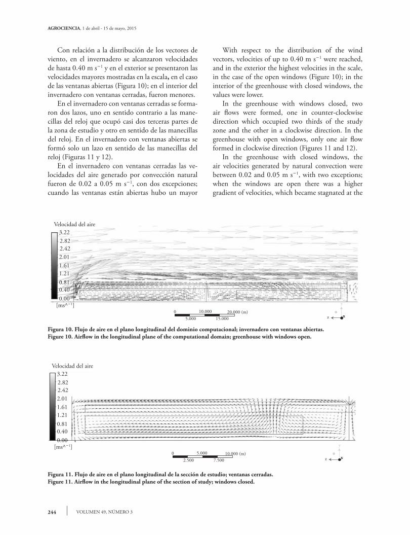
Con relación a la distribución de los vectores de viento, en el invernadero se alcanzaron velocidades de hasta 0.40 m s-1 y en el exterior se presentaron las velocidades mayores mostradas en la escala, en el caso de las ventanas abiertas (Figura 10); en el interior del invernadero con ventanas cerradas, fueron menores.

En el invernadero con ventanas cerradas se forma-ron dos lazos, uno en sentido contrario a las mane-cillas del reloj que ocupó casi dos terceras partes de la zona de estudio y otro en sentido de las manecillas del reloj. En el invernadero con ventanas abiertas se formó solo un lazo en sentido de las manecillas del reloj (Figuras 11 y 12).

En el invernadero con ventanas cerradas las ve-locidades del aire generado por convección natural fueron de 0.02 a 0.05 m s-1, con dos excepciones; cuando las ventanas están abiertas hubo un mayor

Figura 11. Flujo de aire en el plano longitudinal de la sección de estudio; ventanas cerradas.Figure 11. Airflow in the longitudinal plane of the section of study; windows closed.

Velocidad del aire3.22

2.822.422.011.611.21

0.810.40

0.00[ms^1]

0 5.000 10.000 (m)2.500 7.500

y

z x

With respect to the distribution of the wind vectors, velocities of up to 0.40 m s-1 were reached, and in the exterior the highest velocities in the scale, in the case of the open windows (Figure 10); in the interior of the greenhouse with closed windows, the values were lower.

In the greenhouse with windows closed, two air flows were formed, one in counter-clockwise direction which occupied two thirds of the study zone and the other in a clockwise direction. In the greenhouse with open windows, only one air flow formed in clockwise direction (Figures 11 and 12).

In the greenhouse with closed windows, the air velocities generated by natural convection were between 0.02 and 0.05 m s-1, with two exceptions; when the windows are open there was a higher gradient of velocities, which became stagnated at the

Figura 10. Flujo de aire en el plano longitudinal del dominio computacional; invernadero con ventanas abiertas.Figure 10. Airflow in the longitudinal plane of the computational domain; greenhouse with windows open.


2.822.422.01

1.611.21

0.810.40

0.00[ms^1]

0 10.000 20.000 (m)5.000 15.000

y

z x



Figura 12. Flujo de aire en el plano longitudinal de la sección de estudio; ventanas abiertas.Figure 12. Airflow in the longitudinal plane of the section of study; windows open.

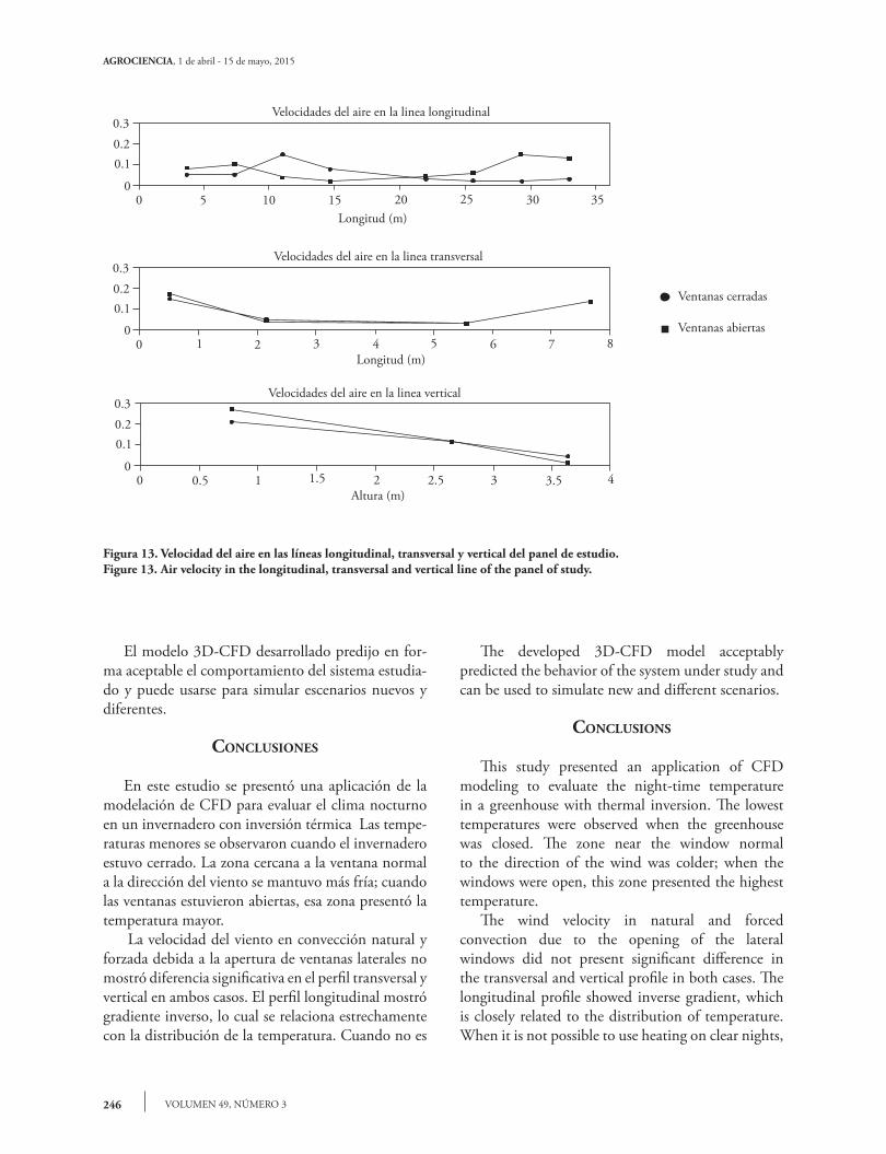
gradiente de velocidades, que se estancó a la mitad de la zona de estudio. En la línea transversal, las ve-locidades mayores se alcanzaron cerca de las ventanas y en el extremo opuesto de ellas. El comportamiento con ventanas cerradas fue similar al de abiertas. En la línea vertical las magnitudes fueron hasta 0.27 m s-1; en ambos casos se observó que a menor altura la velocidad del viento fue mayor (Figura 13).

Según Montero et al. (2005) y Montero et al. (2013), el efecto de inversión térmica en el cual la temperatura del interior del invernadero es menor que la exterior, ocurre en noches con firmamento despejado y es causado por el proceso de enfriamien-to del invernadero porque la cubierta pierde mayor radiación infrarroja que la que recibe de la atmósfera. Castilla (2013) concuerda con lo anterior y agrega que además del factor de noches despejadas, las no-ches sin viento pueden provocar que la inmovilidad del aire dentro del invernadero cause un decremento alto respecto a la temperatura exterior, lo cual resulta en inversión térmica.

En este estudio, ambas explicaciones permiten entender las predicciones del modelo 3D-CFD y las mediciones. La apertura de ventanas permitió el movimiento del aire interno y la diferencia entre la temperatura interna y externa fue menor. El modelo permite probar distintas configuraciones al agregar a las simulaciones de ventanas cerradas y abiertas, el uso de pantallas y cubiertas dobles o el uso de materiales diferentes, como cubierta del invernadero, con el fin de mejorar el ambiente térmico del invernadero. Ade-más, se puede variar la geometría del invernadero, área de ventanas y localización, con la misma finalidad.


2.822.422.011.611.21

0.810.40

0.00[ms^1]

0 5.000 10.000 (m)2.500 7.500

y

z x

middle of the study zone. In the transversal line, the highest velocities were reached in the vicinity of the windows and in the end opposite them. The behavior with closed windows was similar to that of open windows. In the vertical line magnitudes were up to 0.27 m s-1; in both cases it was observed that at a lower altitude, wind velocity was higher (Figure 13).

According to Montero et al. (2005) and Montero et al. (2013), the effect of thermal inversion in which the temperature of the interior of the greenhouse is lower than the exterior, occurs on clear nights and is caused by the cooling process of the greenhouse due to the fact that the greenhouse cover loses more infra-red radiation than it receives from the atmosphere. Castilla (2013) agrees with the above and points out that in addition to the factor of clear nights, windless nights can cause the immobility of the air inside the greenhouse to have a high decrease with respect to the outside temperature, which results in thermal inversion.

In our study, both explanations help to understand both the predictions of the 3D-CFD model and the measurements. The opening of windows permitted the movement of inside air and the difference between the inside and outside temperature was lower. The model makes it possible to test different configurations by adding to the simulations of closed and open windows, the use of screens and double covers or the use of different materials, as greenhouse cover, in order to improve the thermal environment of the greenhouse. Furthermore, the geometry of the greenhouse can vary, along with the area of the windows and their location, with the same purpose.



El modelo 3D-CFD desarrollado predijo en for-ma aceptable el comportamiento del sistema estudia-do y puede usarse para simular escenarios nuevos y diferentes.

conclusIones

En este estudio se presentó una aplicación de la modelación de CFD para evaluar el clima nocturno en un invernadero con inversión térmica Las tempe-raturas menores se observaron cuando el invernadero estuvo cerrado. La zona cercana a la ventana normal a la dirección del viento se mantuvo más fría; cuando las ventanas estuvieron abiertas, esa zona presentó la temperatura mayor. La velocidad del viento en convección natural y forzada debida a la apertura de ventanas laterales no mostró diferencia significativa en el perfil transversal y vertical en ambos casos. El perfil longitudinal mostró gradiente inverso, lo cual se relaciona estrechamente con la distribución de la temperatura. Cuando no es

The developed 3D-CFD model acceptably predicted the behavior of the system under study and can be used to simulate new and different scenarios.

conclusIons

This study presented an application of CFD modeling to evaluate the night-time temperature in a greenhouse with thermal inversion. The lowest temperatures were observed when the greenhouse was closed. The zone near the window normal to the direction of the wind was colder; when the windows were open, this zone presented the highest temperature.

The wind velocity in natural and forced convection due to the opening of the lateral windows did not present significant difference in the transversal and vertical profile in both cases. The longitudinal profile showed inverse gradient, which is closely related to the distribution of temperature. When it is not possible to use heating on clear nights,

Figura 13. Velocidad del aire en las líneas longitudinal, transversal y vertical del panel de estudio.Figure 13. Air velocity in the longitudinal, transversal and vertical line of the panel of study.

0.20.1

00 5 10 15 20 25 30 35

Velocidades del aire en la linea longitudinal

Longitud (m)

Ventanas cerradas

Ventanas abiertas0 1 2 3 4 5 6 7

Longitud (m)8

0 0.5 1 1.5 2 2.5 3 3.5Altura (m)

4

Velocidades del aire en la linea transversal

0

0.3

0.20.1

0.3

0

0.20.1

0.3Velocidades del aire en la linea vertical



posible utilizar calefacción en noches despejadas, se recomienda mantener las ventanas laterales abiertas durante la noche para evitar enfriamiento mayor del interior del invernadero. La comparación de tempe-raturas simuladas y medidas mostró un buen ajuste del código numérico utilizado en este estudio.

lIteRAtuRA cItAdA

ANSYS, Inc. 2013. ANSYS 14.5. Help, Theory Reference, Co-pyright 2013. 945 p.

Castilla, N. 2013. Invernaderos de Plástico: Tecnología y Mane-jo. 2a. ed. Mundi-Prensa. España. pp: 30-33.

Chen, Q. 2009. Ventilation performance prediction for buil-dings: A method overview and recent applications. Building Environ. 44: 848-858.

Flores-Velázquez, J., E. Mejía-Saenz, J. I. Montero-Camacho y A. Rojano. 2011. Análisis numérico del clima interior en un invernadero de tres naves con ventilación mecánica. Agro-ciencia 45: 545-560.

Flores-Velázquez, J., I. L. López-Cruz, E. Mejía-Sáenz e I. Mon-tero-Camacho. 2014. Evaluación del desempeño climático de un invernadero Baticenital del centro de México median-te Dinámica de Fluidos Computacional (CFD). Agrociencia 48: 131-146.

Iglesias, N., J. I. Montero, P. Muñoz, y A. Antón. 2009. Estudio del clima nocturno y el empleo de doble cubierta de techo como alternativa pasiva para aumentar la temperatura noc-turna de los invernaderos utilizando un modelo basado en la Mecánica de Fluidos Computacional (CFD). Hort. Argen-tina 28: 18-23.

Majdoubi, H., T. Boulard, H. Fatnassi, and L. Bouirden. 2009. Airflow and microclimate patterns in a one-hectare Canary type greenhouse: An experimental and CFD assisted study. Agric. For. Meteorol. 149: 1050-1062.

it is recommended to maintain the lateral windows open during the night to avoid greater cooling of the interior of the greenhouse. The comparison of simulated and measured temperatures showed a good fit of the numerical code used in this study.

—End of the English version—

pppvPPP

Mesmoudi, K., S. Bougoul, and P. E. Bournet. 2012. Thermal performance of an unheated greenhouse under semi-arid conditions during the night. Acta Hort. 952: 417-424.

Montero, J.I., P. Muñoz, A. Anton, and N. Iglesias. 2005. Com-putational fluid dynamic modelling of night-time energy fluxes in unheated greenhouses. Acta Hort. 691: 403-410.

Montero, J. I., P. Muñoz, M. C. Sánchez-Guerrero, E. Medrano, D. Piscia, and P. Lorenzo. 2013. Thermal performance of an unheated greenhouse under semi-arid conditions during the night shading screens for the improvement of the night-time climate of unheated greenhouses. Span. J. Agric. Res. 11: 32-46.

Norton, T., D. W. Sun, J. Grant, R. Fallon, and V. Dodd. 2007. Applications of computational fluid dynamics (CFD) in the modelling and design of ventilation systems in the agricultu-ral industry: A review. Bioresource Technol. 98: 2386–2414.

Romero-Gómez, P., C. Y. Choi, and I. L. López-Cruz. 2010. Enhancement of the greenhouse air ventilation rate under climate conditions of central México. Agrociencia 44: 1-15.

Xia, B., and D.-W. Sun. 2002. Applications of computational fluid dynamics (CFD) in the food industry: a review. Com-put. Electron. Agric. 34: 5-24.

determinaciÓn de los gradientes tÉrmicos … · un modelo basado en dinámica de fluidos...

Documents