UNIVERSIDAD DE BUENOS AIRESFacultad de Ciencias Exactas y Naturales

Departamento de Matemática

Métodos combinatorios y algoritmos en topología de dimensiones bajas y laconjetura de Andrews-Curtis.

Tesis presentada para optar al título de Doctor de la Universidad de Buenos Aires en el áreaCiencias Matemáticas.

Ximena Laura Fernández

Director de tesis: Elías Gabriel Minian.Consejero de estudios: Elías Gabriel Minian.

Buenos Aires, 2017.

Métodos combinatorios y algoritmos en topología de dimensiones bajas y laconjetura de Andrews-Curtis

Resumen

En esta Tesis estudiamos la conjetura de Andrews-Curtis desde un nuevo enfoque combina-torio y computacional, utilizando como herramienta principal la teoría de espacios topológicosfinitos.

La conjetura de Andrews Curtis (1965) es uno de los problemas abiertos más relevantes dela topología geométrica, con raíces en la teoría de homotopía simple de Whitehead y la teoríacombinatoria de grupos, de íntima conexión con otros problemas relevantes de la topologíaalgebraica, como la conjetura de asfericidad de Whitehead, la conjetura de Zeeman y la conje-tura (ahora teorema) de Poincaré. Tiene formulaciones equivalentes en el contexto de la teoríacombinatoria de grupos y en el de la topología algebraica en dimensiones bajas. Esencialmenteapunta a reconocer, con métodos discretos, grupos triviales o espacios contráctiles, problemasfrecuentes en topología algebraica y teoría de grupos, que en general no son decidibles com-putacionalmente. Si bien la conjetura se sabe verdadera para cierta clase de complejos (ej,los standard spines, o los complejos cuasi-construibles), ha resultado difícil realizar avancesgenerales. Los abordajes computacionales han resultado limitados por la complejidad expo-nencial en la cantidad de generadores y longitud de las relaciones. Como consecuencia de losresultados de este trabajo, obtenemos una serie de métodos combinatorios y algorítmicos quepermiten reconocer complejos o presentaciones que satisfacen la conjetura, así como tambiénampliar las clases para las cuales la conjetura se sabe cierta.

Nuestro punto de partida fue la construcción de un nuevo modelo finito asociado a unapresentación: un poset fácil de describir en términos de los generadores y relaciones. Desa-rrollamos una serie de métodos de reducción y métodos discretos de transformación de posets.Los últimas están inspirados en técnicas de coloreo de posets, y en teoría de Morse discreta ymatchings acíclicos. Demostramos una versión más fuerte de la teoría de Morse, que precisaequivalencias simples y cotas en las dimensiones los complejos involucrados en la deformación,así como también detalles de las funciones de adjunción. Estas mejoras resultaron esencialespara que la teoría se torne aplicable a nuestro problema.

Estos métodos nos permitieron abordar desde un nuevo punto de vista algunos de los po-tenciales contraejemplos, que consisten de presentaciones balanceadas del grupo trivial paralas cuales no se conoce si satisfacen o no la conjetura. Mostramos que nuestros métodos sonútiles para estudiar presentaciones sin imponer cotas en la longitud de relaciones.

Dada la íntima conexión que existe entre presentaciones y CW complejos de dimensión 2,nuestros resultados se pudieron aplicar también a otros problemas de la topología algebraicaen dimensiones bajas.

Los algoritmos que construimos de reconocimiento de espacios/presentaciones que sat-isfacen la conjetura se encuentran implementados en lenguaje Python, en el marco del soft-ware libre SAGE. El código se encuentra disponible en el siguiente repositorio de GitHub:https://github.com/ximenafernandez/Finite-Spaces.

Palabras clave: conjetura de Andrews-Curtis, espacios topológicos finitos, complejos celu-lares, homotopía simple, presentaciones de grupos, teoría de Morse.

iii

iv

Combinatorial methods and algorithms in low dimensional topology and theAndrews Curtis conjecture

Abstract

In this Thesis we study the Andrews-Curtis conjecture from a new combinatorial and com-putational approach, using as a main tool the theory of finite topological spaces.

The Andrews Curtis conjecture (1965) is one the most relevant open problems in geometrictopology, with roots in Whitehead’s simple homotopy theory and combinatorial group theory,and close relation with other important problems in algebraic topology, such as Whiteheadasphericity conjecture, Zeeman conjecture and the Poincaré conjecture (now a theorem). It hasequivalent statements in the combinatorial group theory context, as well as in the context of lowdimensional topology. It basically aims to recognize, with discrete methods, triviality of groupsor contractibility of spaces, frequent questions in algebraic topology and group theory, whichare computationally undecidable in general. Although the conjecture is known to be true forsome clases of complexes (such as the standard spines or the quasi-constructible complexes), ithas been difficult to obtain general progress. The computational approaches have been shownto be limited by the exponential complexity on the amount of generators and total length of therelators. As a consequence of the results of this work, we obtain a collection of combinatorialand algorithmic methods to recognize complexes or presentations satisfying the conjecture andto increase the classes for which the conjecture is known to be true.

Our starting point is the construction of a new finite model associated to a presentation:a poset easy to describe in terms of the generators and relators. We developed a number ofreduction methods and discrete transformation methods for posets. The last ones are inspired,on the one hand, in coloring techniques of posets and, on the other, in discrete Morse theoryand acyclic matchings. We prove a stronger version of Morse theory, which specifies simplehomotopies and bounds on the dimensions of the involved complexes, as well as details aboutthe adjunction maps. These improvements were essential to make the theory applicable to ourproblem.

These methods allowed us to attack from a new point of view various examples from theclassical list of potential counterexamples, consisting of balanced presentations of the trivialgroup for which it is not known whether the conjecture is satisfied. We show that our methodsare useful to study presentations without imposing bounds on the total length of relators.

Given the close relationship between group presentations and CW complexes of dimension2, our results could be applied to other problems in low dimensional topology.

The algorithms that we constructed for identifying spaces/presentations satisfying the con-jecture, are implemented in Python, using the framework of the free software SAGE. Thesource code is available in https://github.com/ximenafernandez/Finite-Spaces.

Key words: Andrews-Curtis Conjecture, finite topological spaces, cellular complexes, sim-ple homotopy, group presentations, Morse theory.

v

vi

Introducción

Uno de los principales propósitos de la Topología Algebraica es clasificar a los espacios segúnsu tipo homotópico. Se sabe que este problema resulta algorítmicamente indecidible, inclusotrabajando con modelos combinatorios como los complejos simpliciales y una noción másrígida de homotopía: la homotopía simple. Asimismo, el problema de decidir si dos gruposson isomorfos es un problema fundamental en teoría de grupos. Pese a los avances realizadospor Tietze, quien generó una lista corta y efectiva de transformaciones para llevar un grupo acualquier otro isomorfo, este problema también fue probado no resoluble computacionalmenteincluso para grupos finitamente presentados.

Por supuesto, la teoría combinatoria de grupos y la topología crecieron juntas y su conexiónvía el grupo fundamental es bien sabida. Como consecuencia de la interacción de estas teorías,podemos decir que los problemas que mencionamos recién son esencialmente el mismo.

Uno de los principales objetivos de este trabajo es atacar desde un nuevo punto de vistala conjetura de Andrews-Curtis, un problema abierto desde hace 50 años que está íntimamen-te relacionado con las preguntas anteriores. Introducimos novedosos métodos combinatoriosy algoritmos para manipular CW-complejos y presentaciones de grupos preservando su tipohomotópico (simple) y -respectivamente- clase de equivalencia.

Orígenes del problema

En 1965, en su famoso artículo "Free groups and handlebodies" [AC65], James J. Andrews yMorton L. Curtis plantearon una pregunta sobre presentaciones de grupos, generalizando re-sultados previos de Nielsen [Nie18] sobre grupos libres y explicando algunas consecuenciasrelevantes de una posible respuesta afirmativa a su pregunta sobre la (en ese momento abierta)conjetura de Poincaré. El artículo gana relevancia con una observación del referí sobre una ver-sión más débil de la conjetura y su conexión con un problema (a abierto) sobre deformacionesde complejos celulares.

Dado un grupo libre F finitamente generado en x1, · · · , xn, el teorema de Nielsen afirmaque toda otra base y1, · · · , yn de F se puede obtener a partir de x1, · · · , xn aplicando una su-cesión finita de los siguientes movimientos elementales: invertir un elemento, intercambiarelementos, multiplicar un elemento por otro. Ahora, si F es libre en x1, · · · , xn y el conjun-to r1, · · · , rn cumple que su clausura normal es F, entonces no necesariamente será posibletransformar r1, · · · , rn en x1, · · · , xn mediante operaciones de Nielsen. Sin embargo, Andrewsy Curtis conjeturaron que esto sería posible si se permite una cuarta operación: conjugar unelemento por cualquier otro elemento de F. Probaron que, si su conjetura fuera cierta, los en-

vii

tornos regulares de subcomplejos contráctiles de dimensión 2 de 5-variedades combinatoriasserían 5-celdas. Notemos que la conjetura de Andrews-Curtis puede reformularse en términosde presentaciones de grupos. Si P = 〈x1, · · · , xn : r1, · · · , rn〉 es una presentación balanceadadel grupo trivial, definimos como operaciones válidas en la presentación al resultado de aplicarcualquiera de los movimientos definidos por Andrews y Curtis en el conjunto de relaciones.La conjetura afirma que P se puede transformar en 〈x1, · · · , xn : x1, · · · , xn〉 mediante unasucesión finita de operaciones válidas.

El referí sugirió incluir dos nuevas operaciones, que consisten en agregar un nuevo ge-nerador, digamos y, y una nueva relación y, y la operación inversa. Esto llevó a la siguienteconjetura actualmente abierta:

Conjetura (Andrews-Curtis). Si P = 〈x1, · · · , xn|r1, · · · , rn〉 es una presentación balanceadadel grupo trivial, entonces P se puede llevar a la presentación vacía 〈|〉 mediante una sucesiónfinita de las siguientes transformaciones:

• reemplazar ri por r−1i ,

• reemplazar ri por rir j, j , i,

• reemplazar ri por wriw−1, donde w es una palabra en los generadores,

• agregar un nuevo generador y y la relación y, o el inverso de esta operación.

También señaló que esta versión de la conjetura era equivalente a un problema aún abiertosobre deformaciones de complejos celulares y la teoría de homotopía simple de Whitehead: siK es un CW complejo de dimensión 2, ¿se puede expandir a un complejo L de dimensión 3que colapse a un punto? La versión n-dimensional de esta pregunta ya había sido probada paran , 2 por C.T.C. Wall [Wal66b].

Conjetura (Andrews-Curtis, versión topológica). Todo complejo celular finito de dimensión 2contráctil se 3-deforma a un punto.

La generosa sugerencia del referí fue crucial para agregar un punto de vista topológico ala conjetura, que hoy tiene gran importancia. Las dos versiones apuntan a entender desde unenfoque discreto el difícil problema de detectar espacios contráctiles o grupos triviales.

Reseña histórica

Los complejos celulares de dimensión 2 no son tan inocentes como parecen a primera vista.Históricamente, muchos problemas pudieron ser probados (o refutados) en dimensiones altas,pero permanecen aún abiertos en las dimensiones más bajas. La conjetura de Poincaré gene-ralizada es un ejemplo notable de este problema. Ésta fue probada por Stephen Smale paradimensiones mayores a 4 en los 60’s, y por M. Freedman para dimensión 4 en 1982, pero fuerecién en 2002 que Perelman obtuvo una demostración de su validez para dimensión 3.

Muchos problemas vinculados a la topología algebraica de complejos celulares permane-cen aún abiertos para dimensión 2, como la conjetura de asfericidad de Whitehead [Whi41a],la conjetura de Zeeman [Zee64] y la conjetura de Andrews-Curtis [AC65]. La conjetura de

viii

Zeeman implica la conjetura de Andrews-Curtis, y su validez proveería una demostración com-binatoria de la conjetura de Poincaré 3-dimensional. Además, se puede deducir de la conjeturade Poincaré 3-dimensional que ambas conjeturas son ciertas para cierta clase de complejos lla-mados standard spines. Sin embargo, ambas conjeturas permanecen abiertas para complejosen general.

La complejidad de los complejos celulares de dimensión 2 se puede comprender mejor sitenemos en mente su correspondencia con las presentaciones de grupos. Dado un complejocelular conexo de dimensión 2, obtenemos una presentación de su grupo fundamental del si-guiente modo. Se colapsa un árbol generador de su 1-esqueleto y se calcula una presentacióndel grupo fundamental del cociente que se obtiene, que resulta homotópicamente equivalenteal original. Distintas elecciones del árbol, punto base u orientaciones de las celdas dan lugara distintas presentaciones, que se pueden transformar una en otra mediante una sucesión finitade movimientos de Andrews-Curtis. Recíprocamente, una presentación de grupo puede mode-larse como el grupo fundamental de un 2-complejo construido como sigue: comenzar con unaúnica 0-celda, adjuntar una 1-celda por cada generador y darle una orientación, y finalmenteadjuntar una 2-celda por cada relación, con la función de adjunción asociada a la palabra que selee en la relación. Por el teorema de van Kampen, el grupo fundamental de este complejo tienela presentación deseada. Diferentes elecciones de orientación dan lugar a complejos celulares3-deformables (ver [Wri75]).

Esta correspondencia provee numerosas traducciones de problemas de teoría combinato-ria de grupos y computabilidad en problemas de topología algebraica, y viceversa. Algunosejemplos son el problema de la palabra y el problema de isomorfismo:

SeaP = 〈x1, x2, · · · xn : r1, r2, · · · , rm〉 una presentación de un grupo finitamente presentadoG. Si w es una palabra en los generadores, ¿es w trivial en G? ¿Es G el grupo trivial?

En 1911, Max Dehn cuestionó la existencia de algoritmos que respondan las preguntasanteriores para grupos en general, y produjo algoritmos que las responden para grupos fun-damentales de 2-variedades cerradas orientables. Reconoció una característica crucial en estosgrupos: están definidos por relaciones con propiedades de cancelación pequeña, dando lugar ala teoría de pequeña cancelación. Lo métodos de Dehn eran geométricos, hacía uso de tesela-ciones regulares del plano hiperbólico, y sus algoritmos se extendieron a una amplia clase degrupos [Deh11]. Sin embargo, él mismo conjeturó que el problema general era no decidible.En efecto, con la formalización de las nociones de algoritmo y computabilidad realizadas porTuring en los 30’s [Tur37], Novikov [Nov55] y Boone [Boo54a, Boo54b, Boo55a, Boo55b]lograron hallar un grupo finitamente presentado G para el cual el problema de la palabra es nodecidible. Más tarde, Adian y Rabin [Adi93, Rab58] probaron que, en general, no es decidibleel problema de determinar si una presentación define el grupo trivial. Sin embargo, no se sabeaún si es decidible este problema para presentaciones balanceadas. No obstante, recientementefue probado por Gadgil [Gad01] que si la conjetura de Andrews-Curtis fuera cierta, entoncesefectivamente existiría un algoritmo para decidir si una presentación balanceada define el grupotrivial.

Vía la correspondencia de presentaciones de grupo con 2-complejos celulares, hay unatraducción de los problemas anteriores en el marco topológico algebraico.

ix

Sea K un complejo celular arcoconexo finito de dimensión 2. Si α es un lazo en K, ¿es αtrivial? ¿Es K simplemente conexo? ¿Es K contráctil?

Es claro que las primeras dos preguntas son problemas topológicos no decidibles, y que laúltima pregunta sería decidible si la conjetura de Andrews-Curtis fuera cierta [Gad01].

A pesar de que determinar si un grupo es trivial o un espacio es contráctil son problemas notratables computacionalmente, han surgido varios abordajes que enfrentan el problema desdeun punto de vista discreto. Los principales ejemplos son la teoría de Tietze para grupos y lateoría de Whitehead para complejos celulares.

En 1908, Tietze [Tie08] mostró que dadas dos presentaciones finitas de un mismo grupo, sepueden obtener una de la otra mediante una secuencia finita de cierta lista de transformacioneselementales. Las transformaciones de Tietze permiten: invertir una relación, multiplicar unarelación por otra, conjugar una relación por otro elemento en el grupo libre de generadores,agregar un nuevo generador y una nueva relación igual al generador agregado (y la operacióninversa), y agregar una nueva relación igual a un generador ya existente (y la operación in-versa). Notar que cada una de las operaciones previas en la presentación de grupo preservan laclase de isomorfismo, pero no todas mantienen el tipo homotópico del complejo celular aso-ciado. Las primeras cuatro son justamente los movimientos de Andrews-Curtis, y se puedeninterpretar topológicamente como cambiar la función de adjunción de la celda asociada a larelación por una homotópica, lo cual no cambia el tipo homotópico simple. Agregar un nue-vo generador y una relación igual al generador agregado es justamente la operación sugeridapor el referí, y significa una expansión elemental en el complejo celular. Finalmente, la últimatransformación se traduce en la adjunción de una esfera que cambia el tipo homotópico perono altera el grupo fundamental. La conjetura de Andrews-Curtis dice entonces que se puedeprescindir del último movimiento de Tietze en presentaciones balanceadas del grupo trivial.

Como una simple consecuencia del teorema de Whitehead, se puede ver que las presenta-ciones balanceadas del grupo trivial se corresponden 1-1 con complejos celulares de dimen-sión 2 contráctiles. Más aún, se puede ver que los movimientos de Andrews-Curtis se corres-ponden con 3-deformaciones de complejos celulares.

La teoría de homotopía simple de Whitehead es el análogo topológico de la teoría de Tietzepara presentaciones de grupos, dando un enfoque combinatorio al clásico problema de clasifi-cación de tipos homotópicos. Sus contribuciones [Whi41b, Whi50] resultaron ser fundamenta-les para el desarrollo de la topología lineal a trozos y la geometría combinatoria. Algunos desus principales logros y aplicaciones son: el teorema de s-cobordismo, la conjetura de Zeeman[Zee64], la conjetura de Andrews-Curtis [AC65], las aplicaciones a la teoría de cirugía, el clá-sico artículo de Milnor sobre la torsión de Whitehead [Mil66], la invariancia topológica de latorsión.

De manera similar al caso de las transformaciones elementales de Tietze, Whitehead cons-truyó su teoría sobre dos movimientos elementales de deformación sobre complejos celularesque preservan su tipo homotópico: las expansiones y los colapsos. Una sucesión finita de co-lapsos y expansiones es una deformación formal, que da lugar a la noción de homotopía simple.Uno podría preguntarse cuándo es cierto una suerte de análogo del teorema de Tietze, es decir,cuándo dos complejos homotópicamente equivalentes se pueden conectar mediante una cade-na de expansiones y colapsos. Desafortunadamente, esto no se puede lograr en general. De

x

hecho, existe una obstrucción algebraica, hoy llamada el grupo de Whitehead, que cuantificala brecha. Si el grupo de Whitehead Wh(K) de un complejo celular K es trivial, entonces todocomplejo homotópicamente equivalente a K es simplemente equivalente a K. En particular,como el grupo de Whitehead de los complejos contráctiles es trivial, entonces todo complejocontráctil se puede transformar en un punto mediante una sucesión finita de expansiones y co-lapsos. Más aún, si el complejo tiene dimensión n , 2, existe una deformación en la cual loscomplejos involucrados tienen dimensión a lo sumo n + 1 [Wal66b]. La pregunta para n = 2aún se encuentra abierta y es la conjetura de Andrews-Curtis.

Recientemente, el desarrollo de la teoría de homotopía de espacios finitos [Bar11a] pro-porcionó un nuevo enfoque combinatorio a muchos problemas de la topología algebraica. Losespacios topológicos finitos son una herramienta doble: por un lado, son modelos finitos decomplejos celulares regulares; por el otro, se pueden pensar como posets finitos, un objeto ma-nejable que permite hacer fácilmente los cálculos. Para cada complejo celular regular K, existeun espacio topológico finito X(K) con el mismo tipo homotópico débil. El tipo homotópico(fuerte) de los espacios finitos está completamente determinado por un algoritmo goloso decomplejidad polinomial, que consiste en remover uno a uno puntos del diagrama de Hasse concierta característica combinatoria (que el grado de entrada o el de salida sea igual a 1) [Sto66].En cambio, clasificar el tipo homotópico débil de espacios finitos es tan difícil como clasificarel tipo homotópico de espacios topológicos en general, es decir, no es decidible computacio-nalmente. En [BM08b], Barmak y Minian desarrollaron un análogo de la teoría de homotopíasimple para espacios finitos, de modo que K se (n + 1)-deforma a L si y sólo si X(K) se (n + 1)-deforma aX(L). Las deformaciones de espacios finitos también están también definidas a travésde dos movimientos elementales: los colapsos y sus inversos, las expansiones. Pero esta vez,un colapso elemental es simplemente remover un vértice con cierta característica combinatoria:que el conjunto de puntos comparables distintos sea contráctil. Luego, se obtiene una versióncombinatoria de la conjetura.

Conjetura (Andrews-Curtis, versión espacios finitos). Si X es un espacio topológico finitohomotópicamente trivial de altura 2, entonces X se 3-deforma a un punto.

Además, los autores introducen las qc-reducciones y hallan una gran clase de complejossimpliciales, los qc-construibles, que satisfacen la conjetura.

A lo largo de los últimos 50 años, se ha construido una lista de ejemplos de presentacionesbalanceadas del grupo trivial para los cuales no se conoce trivialización vía movimientos deAndrews-Curtis. Sirven como potenciales contraejemplos de la conjetura.

(i) 〈x, y|xy2x−1 = y3, yx2y−1 = x3〉, Crowell & Fox (1963) [CF77, p.41].

(ii) 〈x, y, z|z−1yz = y2, x−1zx = z2, y−1xy = x2〉, Rapaport (1968) [Rap68a].

(iii) 〈x, y|x = [xm, yn], y = [xp, yq]〉, m, n, p, q ∈ Z, Gordon (1984) [Bro84].

(iv) 〈x, y|xyx = yxy, x4 = y5〉, Akbulut & Kirby (1985) [AK85].

A continuación, hacemos un pequeño resumen y comentarios sobre sus orígenes y el trabajopreviamente realizado en torno a estos ejemplos.

xi

El ejemplo (i) está contenido en una serie más general de presentaciones balanceadasdel grupo trivial que se encuentra en un artículo más reciente de Miller y Schupp [MS99]:〈x, y|yxnby−1 = xn+1, y = w〉, donde n ≥ 1, y w es una palabra en x e y de modo que losexponentes de las y suman 0.

El ejemplo (ii) pertenece a una serie de presentaciones con n generadores xi, y relacionescíclicamente indexadas x−1

i+1xixi+1 = x2i . Para n = 2, la presentación se puede trivializar fá-

cilmente con transformaciones de Andrews-Curtis. Para n = 3, se puede transformar en unapresentación de 2 generadores y 2 relaciones, aunque esta “reducción” incrementa la longitudde las relaciones. Para n > 4, la presentación corresponde a grupos infinitos no triviales.

El ejemplo (iii) fue encontrado por Gordon y comunicado por Lickorish a Ronald Brown,quien lo incluyó en su artículo [Bro84] con el permiso del creador. En [BM06] se probó quelas presentaciones de esta serie cuya longitud total de relaciones es igual a 14 satisfacen laconjetura de Andrews-Curtis.

El ejemplo (iv) es el más estudiado. Surge a partir de una descomposición en manijas de la4-esfera de Akbulut-Kirby [AK85]. Todas las presentaciones de la familia 〈x, y|xyx = yxy, xn =

yn+1〉 corresponden al grupo trivial. Para n > 2, no se sabe si son Andrews-Curtis trivializables.Para n = 2, Gersten mostró en 1982 que trivializable con movimientos de Andrews-Curtis.Sin embargo, el artículo no se encuentra publicado. No fue hasta varios años después que Ha-vas & Ramsay [HR03] y Miasnikov [Mia99, MM01] muestran trivializaciones concretas. Parahallarlas, Miasnikov creó nuevos algoritmos genéticos diseñados para testear la validez de laconjetura. Su principal resultado dice que todas las presentaciones balanceadas del grupo trivialcuya longitud total de las relaciones es a lo sumo 12 satisfacen la conjetura. Usaron el softwarecomputacional MAGNUS. Por su parte, Havas & Ramsay exhibieron un abordaje computacio-nal basado en un breadth-first search sobre el árbol de presentaciones AC-equivalentes. Desa-rrollaron el software libre ACME. Para n = 3, no se lograron obtener resultados con ningunode los algoritmos anteriores. En realidad, los enfoques anteriores tienen el mismo púnto débil:tratan de exhibir explícitamente la sucesión de movimientos que llevan a una presentación a lapresentación trivial. Recientemente, en 2015, Bridson [Bri15] halló ejemplos de presentacionesbalanceadas del grupo trivial, que son trivializables mediante movimientos de Andrews-Curtis,pero que la cantidad mínima de transformaciones requeridas para lograrlo crece más rápidoque cualquier torre de exponenciales. Los ejemplos están construidos con la idea de codificaren presentaciones balanceadas la complejidad del problema de la palabra de ciertos grupos.

Contribuciones

Hasta ahora, no se conocen métodos para manejar las 3-deformaciones algorítmicamente. Eneste trabajo, proponemos una nueva estrategia para estudiarlas: introducimos nuevos méto-dos de reducción de espacios finitos, que codifican una 3-deformación de dos pasos. Esto es,X↗ Y↘ ∗, donde la altura de Y es menor o igual que 3. Cada reducción decrece el número depuntos o aristas del diagrama de Hasse asociado al poset, y se puede describir fácilmente entérminos de la combinatoria de este grafo. Algunos ejemplos de los nuevos métodos desarrolla-dos son: las reducciones de arista, las middle reducciones, y varios otros tipos de reduccionesde tipo cociente, incluyendo las O-reducciones, una generalización y mejora de los métodos dereducción de Osaki [Osa99] para tipos homotópicos débiles de espacios finitos. Estos métodos

xii

proveen una técnica algorítmica (no exhaustiva) para mostrar que un espacio se 3-deforma a unpunto, dando lugar a la caracterización de nuevas clases de espacios que satisfacen la conjetura.

La principal herramienta que usamos para las demostraciones es una generalización arelaciones en general del cilindro no-Hausdorff de una función: construimos el cilindro no-Hausdorff de una relación, que denotamos BR.

Corolario 3.1.4. Sea R ⊆ X × Y una relación entre espacios topológicos finitos. Si R−1(Uy)

y R(Fx) son homotópicamente triviales para cada x ∈ X e y ∈ Y, entonces K(X)�↘ K(Y).Más aún, si R(Fx), R−1(Uy) son colapsables, entonces K(X)�↘n K(Y), deonde n es la alturadel cilindro.

Los nuevos métodos de reducción que formulamos en esta tesis para estudiar la conjeturade Andrews-Curtis son descriptos en los siguientes resultados.

Las middle-reducciones son una variación de las qc-reducciones para puntos que no sonmaximales ni minimales, que satisfacen ciertas condiciones.

Proposición 3.2.7. Sea X un espacio finito de altura a lo sumo 2. Si hay una middle-reducciónde X a X/{a,b}, entonces X �↘3 X/{a,b}.

Las reducciones de arista son reducciones de cierto tipo de arcos del diagrama de Hasse deun espacio finito.

Proposición 3.2.12. Sea X un espacio finito de altura a lo sumo 2. Sea e = (a ≺ b) una aristatal que existe una reducción de X a X r e. Entonces X �↘3 X r e.

Un resultado relevante fue la prueba de que las reducciones de Osaki [Osa99] en espaciosde dimensión 2 son 3-deformaciones.

Teorema 3.2.15. Sea X un espacio finito de altura n y sea x0 ∈ X. Si Ux ∩ Ux0 es vacío ocontráctil para todo x ∈ X, entonces X �↘

n+1X/Ux0 .

En general, un espacio finito X no tiene el mismo tipo homotópico débil que sus cocientesX/A, incluso si A es contráctil. Hallamos una condición general sobre A que asegura que si Xes de altura n, entonces X �↘

n+1X/A.

Teorema 3.2.19. Sean X un espacio finito de altura n, A ⊆ X un subespacio abierto conexo.Si A es homotópicamente trivial, entonces X �↘ X/A. Más aún, si A es colapsable, entoncesX �↘

n+1X/A.

Mostramos también que el cilindro de una relación es útil para el estudio de varios otrosproblemas de la topología algebraica con métodos combinatorios, como clasificar el tipo ho-motópico de colímites homotópicos [FM16], generalizar el Teorema del Nervio [FM17].

El siguiente resultado es una generalización del clásico Teorema del Nervio (probado ori-ginalmente por Borsuk [Bor48], con versiones más generales de Björner[Bj"03] y Barmak[Bar11b]), en la cual permitimos al cubrimiento tener intersecciones no vacías no contráctiles.

DadoU un cubrimiento finito por abiertos X, el nervio no-Hausdorff deU es el face posetdel nervio clásico N(U). Lo denotamos por N(U).

xiii

Teorema 4.1.4. Sea X un espacio topológico finito y sea U = {Ui}i∈I un cubrimiento abiertode X. Sea N0(U) el subespacio del nervio no-Hausdorff N(U) de todas las intersecciones ho-motópicamente triviales. Si para todo x ∈ X, el subespacio Ix de N0(U) de las interseccionesque contienen a x, es homotópicamente trivial, entonces X tiene el mismo tipo homotópicosimple que N0(U).

Decimos que una familiaU de subespacios de un espacio finito X es un cubrimiento cuasi-bueno si toda intersección no vacía de una subfamilia de U tiene sus componentes conexashomotópicamente triviales. A partir de cubrimientos cuasi-buenos, se pueden construir cubri-mientos que satisfagan las hipótesis del Teorema 4.1.4. Denotamos por M(U) al espacio finitocuyos elementos son las componentes conexas del espacio finito cuyos elementos son las com-ponentes conexas de cada intersección de elementos deU, con el orden dado por la inclusión.

Corolario 4.1.9. Sea X un espacio finito y seaU un cubrimiento cuasi-bueno de X. Entonces,X �↘ M(U).

Por otra parte, introdujimos un modelo finito de colímites homotópicos y usamos la cons-trucción del cilindro de una relación y un teorema clásico de McCord para probar una genera-lización del célebre Teorema de Thomason [Tho79] en el contexto de colímites homotópicossobre posets. También obtuvimos análogos de resultados conocidos, como el Teorema Cofi-nal [BK72, Vog73] y una generalización de Teorema A de Quillen para posets [Qui72]. Enparticular, esto permitió caracterizar los colímites homotópicos de diagramas de complejossimpliciales en términos de la construcción de Grothendieck de diagramas de sus face posets.Estos resultados aparecieron en [FM16].

Dado X : P → P<∞ un diagrama de posets finitos indexado en un poset, definimoshocolim X, el colímite homotópico no-Hausdorff de X, como su construcción de GrothendieckP

∫X, la cual resulta también un poset fácil de describir.Tratamos a la construcción de Grothendieck de diagramas de posets como un espacio fi-

nito, y usamos un teorema de McCord para inferir en el contexto combinatorio, resultados alos conocidos sobre colímites homotópicos, y para probar una generalización del teorema deThomason. Esta generalización nos permitió aplicar métodos de reducción para estudiar el tipohomotópico de diagramas de poliedros (indexados en posets finitos).

El Teorema A de Quillen para posets se sigue inmediatamente de las siguientes proposicio-nes, aplicando los resultados al poset 1, con elementos 0 < 1.

Proposición 5.3.1. Sea X : P → P<∞ un P diagrama de espacios finitos. Si p ∈ P es un upbeat point, entonces hocolim X↘↘ hocolim X|Pr{p}.

Proposición 5.3.5. Sea X : P → P<∞ un P diagrama de espacios finitos. Si p un down beatpoint de P dominado por q y f −1

qp (Ux) es contráctil para cada x ∈ Xp, entonces

hocolim X↘ hocolim X|Pr{p}

El principal resultado de esta parte es la siguiente generalización del teorema de Thomasonen el contexto de espacios finitos.

xiv

Teorema 5.4.1. Sea P un poset finito. Sea K : P → Top un diagrama de espacios y X : P →P<∞ un diagrama de posets finitos. Sea φ : K → Top un morfismo de diagramas (donde X esvisto como diagrama de espacios topológicos finitos) tal que φp : Kp → Xp es una equivalenciahomotópica débil para cada p ∈ P. Entonces, existe una equivalencia homotópica débil

ϕ : hocolim K → hocolim X

entre el colímite homotópico de K al colímite homotópico no-Hausdorff de X (visto comoespacio topológico finito).

Como consecuencia directa de este resultado, obtuvimos por un lado un caso particulardel teorema de Thomason en el contexto de posets, y por el otro, una suerte de recíproca delteorema de Thomason, que relaciona el colímite homotópico de un diagrama de complejossimpliciales con el colímite homotópico no-Hausdorff del diagrama de sus face posets. Comocorolario del Teorema 5.4.1, pudimos probar también la invariancia por subdivisión baricéntricadel tipo homotópico de colímites homotópicos de complejos simpliciales en el caso general (nonecesariamente ordenado). La teoría desarrollada permite simplificar en general el cálculo decolímites homotópicos de espacios.

Por otra parte, también desarrollamos otro ataque combinatorio distinto de la conjetura deAndrews-Curtis, esta vez haciendo una nueva interpretación de su versión para presentacionesde grupos. Dada una presentación balanceada del grupo trivial, elaboramos dos técnicas paratransformarla en una nueva presentación que puede obtenerse de la original vía una sucesiónde movimientos de Andrews-Curtis, pero sin especificar la lista explícita de movimientos quellevan de una a la otra. Dada una presentación P del grupo G, denotamos XP al face posetde la subdivisión baricéntrica del CW-complejo asociado a la presentación. Claraemnte, esteposet tiene su grupo fundamental isomorfo a G, y su diagrama de Hasse puede ser descriptofácilmente en términos de P.

Una de las técnicas desarrolladas está inspirada en la teoría de coloreo de posets y es, dehecho, una generalización e implementación discreta del hecho de que colapsar un árbol enel 1-esqueleto de un 2-complejo celular es una 3-deformación. Dado X un poset finito y Aun subdiagrama colapsable de X que contiene todos sus puntos, construimos una presentaciónPX,A del grupo fundamental de X, que resulta AC-equivalente a PK(X). Como consecuencia,obtuvimos el siguiente

Teorema 6.3.1. Si P es una presentación de grupo y A es un subdiagrama generador colap-sable deH(XP), entonces P ∼AC PXP,A.

La otra técnica que desarrollamos está inspirada en la teoría de Morse discreta, introducidapor Robin Forman [For98] en los ’90s como una versión combinatoria de la teoría clásicapara variedades diferenciables. Obtuvimos una versión más fuerte del teorema principal dela teoría de Morse, haciendo la teoría ahora aplicable a nuestro contexto. Nuestro resultadotiene la ventaja de describir más precisamente la equivalencia homotópica. Mostramos queuna función de Morse (o, equivalentemente, un matching M en el diagrama de Hasse del faceposet del complejo) induce no sólo una equivalencia homotópica, sino también una (n + 1)-deformación entre el compleho celular (de dimensión n) y el complejo de Morse KM. También

xv

hicimos precisa la descripción de este complejo, describiendo las funciones de adjunción desus celdas y no sólo la cantidad de celdas de cada dimensión.

Teorema 6.4.17. Sea K un complejo celular regular de dimensión n y sea M un matchingacíclico enH(X(K)). Entonces K �↘

n+1KM.

Dimos una descripción explícita de la presentación estándar de KM, que denotamos porQX(K),M.

Corolario 6.5.6. Sea K un complejo celular regular de dimensión 2, y sea M un matchingacíclico en H(X(K)) con una sola celda crítica de dimensión 0. Entonces QX(K),M es unapresentación balanceada de π1(K) . Más aún, QX(K),M ∼AC PK .

A partir de las estrategias anteriores desarrollamos algoritmos concretos para obtener pre-sentaciones AC-equivalentes, evitando tener que exhibir la lista de movimientos necesariospara lograr tal transformación, lo cual es un avance considerable a la luz de los resultados de[Bri15]. Bajo este enfoque, obtuvimos, entre otras, demostraciones simples de los siguienteshechos sobre la lista de potenciales contraejemplos.

• La presentación 〈x, y|xyx = yxy, xn = yn+1〉 [AK85] para n = 2, satisface la conjetura deAndrews-Curtis.

• La presentación 〈x, y, z|z−1yz = y2, x−1zx = z2, y−1xy = x2〉 [Rap68a], se puede trasfor-mar en una presentación con 2 generadores y 2 relaciones.

• Hay una gran clase de enteros n,m, p, q para la cual la presentación 〈x, y|x = [xm, yn], y =

[xp, yq]〉 [Bro84] satisface la conjetura.

Nuestros métodos se pueden manejar fácilmente con una computadora. Implementamostodos los algoritmos que existían sobre espacios finitos [Fer11] y los nuevos que desarrollamosen esta tesis usando el software libre SAGE [S+17]. Creamos un módulo anexable a SAGE (verApéndices 2.A, 3.A y 6.A) que permite trabajar con espacios finitos y sus aplicaciones, inclu-yendo el estudio de presentaciones de grupos y complejos celulares. El código está disponibleen https://github.com/ximenafernandez/Finite-Spaces.

Descripción de los capítulos

La tesis está organizada en seis capítulos. En el primer capítulo hacemos una reseña históri-ca del problema. Analizamos los distintos enfoques existentes y los estudiamos en un marcounificado. En el segundo capítulo, explicamos el punto de vista combinatorio bajo el cual tra-bajaremos en los siguientes capítulos. Describimos la conexión entre complejos celulares re-gulares, espacios topológicos finitos y posets. Explicamos la teoría de homotopía simple paraespacios finitos y la reformulación de la conjetura de Andrews-Curtis desde esta perspectiva. Eltercer capítulo introduce los nuevos métodos combinatorios en espacios finitos que desarrolla-mos para estudiar 3-deformaciones, y sus aplicaciones al estudio de la versión de la conjeturapara espacios finitos y otros problemas de la topología algebraica. El cuarto capítulo muestranuevas versiones del clásico teorema del Nervio, y aplicaciones al estudio de 3-deformaciones.

xvi

El quinto capítulo trata de colímites homotópicos. En el sexto capítulo, desarrollamos nuevosmétodos combinatorios para presentaciones de grupos, y sus aplicaciones al estudio de los po-tenciales contraejemplos. Casi todos los resultados de los capítulos 3, 4, 5 y 6 son nuevos yoriginales. Algunos de los resultados de los capítulos 3, 4 y 5 aparecieron en [FM16, FM17].Los resultados del capítulo 6 no están publicados aún y serán objeto de un próximo artículo[Fer17].

xvii

xviii

Introduction

The classification of spaces up to homotopy equivalence is one of the primary objectives ofAlgebraic Topology. This problem is known to be algorithmically undecidable, even restrictedto combinatorial models such as simplicial complexes with a more rigid notion of homotopy,the simple homotopy. Likewise, deciding whether two groups are isomorphic is a fundamentalproblem in group theory. Despite the efforts of Tietze to produce a short effective list of trans-formations, this problem was also proved to be unsolvable even for finitely presented groups.Of course, combinatorial group theory and topology grew up together and their connectionvia the fundamental group is well known. As a consequence of the interaction between thesetheories, one could say that the problems mentioned above are essentially the same.

One of the main goals of this work is to attack from a new point of view the Andrews-Curtisconjecture, a fifty-year old open problem which is closely related to the preceding problems.We introduce novel combinatorial methods and algorithmic procedures to manipulate CW-complexes and group presentations preserving their (simple) homotopy type and -respectively-equivalence class.

Origins of the problem

In 1965, in their famous article "Free groups and handlebodies" [AC65], J.J. Andrews and M.L. Curtis raised a question about presentations of groups, generalizing previous ideas of Nielsen[Nie18] about free groups and accounting for some relevant topological consequences of apossible affirmative answer of their question to the (at that time open) Poincaré conjecture. Thearticle increased its relevance with the referee’s remark on a weakening of the conjecture andits relationship with a (also open) homotopical problem concerning deformations of cellularcomplexes.

Given a finitely generated free group F on x1, · · · , xn, Nielsen’s theorem asserts that anyother basis y1, · · · , yn of F can be obtained from x1, · · · , xn by applying a finite sequence ofthe following elementary moves: inverting one element, interchanging elements, multiplyingan element by another one. Now, if F is free on x1, · · · , xn, and the set r1, · · · , rn is such that itsnormal closure is F, then it may not be possible to change r1, · · · , rn to x1, · · · , xn by Nielsenoperations. However, Andrews and Curtis conjectured that this should be possible if a fourthoperation is allowed: conjugating an element by any element of F. They proved that if theirconjecture were true, regular neighbourhoods of contractible 2-dimensional subcomplexes ofcombinatorial 5-manifolds would be 5-cells. Notice that the Andrews-Curtis conjecture canbe reformulated in terms of group presentations. For P = 〈x1, · · · , xn : r1, · · · , rn〉 a balanced

xix

presentation of the trivial group, define a valid operation on this presentation to be the result ofapplying any of the moves already defined by Andrews and Curtis on the set of relators. Theconjecture states that P can be transformed in 〈x1, · · · , xn : x1, · · · , xn〉 by a finite sequence ofvalid operations.

The referee suggested to include two new operations, consisting of adding a new generator,say y, and the additional relator y; and also the inverse of the previous procedure; giving rise tothe following open problem:

Conjecture (Andrews-Curtis). If P = 〈x1, · · · , xn | r1, · · · , rn〉 is a balanced presentation ofthe trivial group, then P can be transformed in the empty presentation 〈 | 〉 by a finite sequenceof the following transformations:

• replace some ri by r−1i ,

• replace some ri by rir j, j , i,

• replace some ri by wriw−1, where w is any word in the generators,

• introduce a new generator y and the relator y; or the inverse of this operation.

He also pointed out that this version of the conjecture was equivalent to a still open problemabout deformations of cellular complexes of dimension 2 and Whitehead’s simple homotopytheory: given K a contractible cellular complex of dimension 2 , is it possible to expand K toa 3-dimensional cellular complex L which collapses to a point? Note that the n-dimensionalversion of this statement had already been proved for n , 2 by C.T.C. Wall [Wal66b].

Conjecture (Andrews-Curtis, topological version). If K is a contractible finite cellular com-plex of dimension 2, then K 3-deforms to a point.

The generous remark of the referee was crucial in adding a new topological point of view tothe conjecture, which nowadays has a great importance. Both versions of the conjecture are anattempt to understand from a discrete point of view the hard problem of detecting contractiblespaces or trivial groups.

Historical overview

Cellular complexes of dimension two are not as innocent as they seem at first glance. Histor-ically, many problems have been proved (or disproved) in higher dimensions but they remainopen in lower ones. The generalized Poincaré conjecture is a notable example of such a prob-lem. Proved by Stephen Smale for dimensions greater than 4 in the sixties and by M. Freedmanfor dimension 4 in 1982, it was not until the late 2002 that Perelman obtained a proof of itsvalidity for dimension 3.

Many problems related to the algebraic topology of the cellular complexes are still openfor dimension 2, such as the Whitehead asphericity conjecture [Whi41a], the Zeeman conjec-ture [Zee64] and the Andrews-Curtis conjecture [AC65]. The Zeeman conjecture implies theAndrews-Curtis conjecture, and its validity would provide an alternative combinatorial proof ofthe 3-dimensional Poincaré conjecture. Furthermore, it can be deduced from the 3-dimensional

xx

Poincaré conjecture that both Zeeman and Andrews-Curtis conjectures are true for some classof complexes called standard spines. However, both conjectures are still open for generalcomplexes.

The complexity of the cellular complexes of dimension 2 can be better understood by keep-ing in mind their correspondence with group presentations. Given a connected cellular complexof dimension 2 it is possible to obtain a presentation of its fundamental group as follows. Co-llapse a spanning tree of the 1-skeleton and compute the presentation of the fundamental groupof the resulting homotopy equivalent quotient space. Different choices of the tree, the basepoint or the orientation of the cells lead to different presentations, which can be transformedone in each other by a sequence of Andrews-Curtis moves. Reciprocally, a group presentationis modeled by a two-complex constructed as follows: start with one 0-cell, attach one 1-cellfor every generator and give an orientation to each one, and finally attach one 2-cell for ev-ery relator, with attaching map spelling the word associated to the relator. By the van Kampentheorem, the fundamental group of this complex has the desired presentation. Different choicesof orientations results in 3-deformable cellular complexes (see [Wri75]).

This correspondence leads to many translations of problems in combinatorial group theoryand computability into the algebraic topology side, and vice-versa. Very first examples wouldbe the word problem and the isomorphism problem:

Let P = 〈x1, x2, · · · xn | r1, r2, · · · , rm〉 be a presentation of a finitely presented group G. If wis a word on the generators, is w trivial in G? Is G the trivial group?

In 1911, Max Dehn posed the existence of algorithms answering the previous questionsfor groups in general, and provided algorithms solving them for fundamental groups of closedorientable 2-dimensional manifolds. He recognized a crucial feature of these groups: they aredefined by relations with small cancellation properties, giving rise to the small cancellationtheory. Dehn’s methods were geometric, making use of regular tessellations of the hyperbolicplane, and their algorithms have been extended to large classes of groups [Deh11]. However,he conjectured that the general problem was undecidable. Indeed, with the formalization of thenotions of algorithm and computability due to Turing in the 1930s [Tur37], Novikov [Nov55]and Boone [Boo54a, Boo54b, Boo55a, Boo55b] found a finitely presented group G such thatthe word problem in G is undecidable. Later, Adian and Rabin [Adi93, Rab58] proved that it isundecidable whether a finite presentation defines the trivial group. However, the decidability ofthis problem for balanced presentations is not settled. It was recently proved by Gadgil [Gad01]that if the Andrews-Curtis conjecture were true, there would actually exist an algorithm todecide if a balanced presentation defines the trivial group.

Via the correspondence of group presentations with 2-dimensional cellular complexes,there is a translation of the previous problems in the algebraic topology setting.

Let K be a finite path-connected cellular complex of dimension 2. If α is a loop in K, is αtrivial? Is K simply connected? Is K contractible?

It is clear that the fist two questions are undecidable topological problems, but it was provedthat the last one would be decidable if the geometric Andrews Curtis conjecture were true[Gad01].

xxi

Although determining the triviality of groups or contractibility of spaces is intractable,different approaches to deal with these problems from a discrete point of view have been pur-sued. The main examples are the Tietze theory for groups and the Whitehead theory for cellularcomplexes.

In 1908, Tietze [Tie08] showed that any two finite presentations of the same group canbe obtained from the other by a finite sequence of certain list of elementary transformations.Tietze transformations allow: to invert a relation, to multiply a relation by another one, toconjugate a relation by any element in the free group on the generators, to add an additionalgenerator and a relation equal to the added generator (and the inverse operation), and to adda new relation equal to an already existing generator (and the inverse operation). Notice thateach of the previous operations on the group presentation preserves the isomorphism type, butnot all of them maintain the homotopy type of the associated cellular complex. The first fouroperations are precisely Andrews-Curtis moves, and they can be topologically seen as changingthe attaching map of the cell associated to the relation involved by a homotopic one, which doesnot change the simple homotopy type. Adding a new generator and a relation equal to the addedgenerator is the referee’s suggested operation, which amounts to an elementary expansion onthe cellular complexes. Finally the last transformation implies the attaching of a sphere, whichchanges the homotopy type but leaves the fundamental group unaltered. The Andrews-Curtisconjecture states that the last Tietze move is not necessary for balanced presentations of thetrivial group.

As a simple consequence of Whitehead’s theorem, one can see that balanced presentationsof the trivial group are in one to one correspondence with contractible cellular complexesof dimension 2. Moreover, it can be proved that the Andrews-Curtis moves correspond to 3-deformations of the cellular complexes.

Whitehead’s simple homotopy theory is the topological analogue of Tietze’s theory forgroup presentations, providing a combinatorial approach of the classical problem of classifica-tion of homotopy types. His contributions [Whi41b, Whi50] turned out to be fundamental forthe development of piecewise-linear topology and combinatorial geometry. Some of the mainachievements and applications are: the s-cobordism theorem, Zeeman’s conjecture [Zee64], theAndrews-Curtis conjecture [AC65], the applications of the theory in surgery, Milnor’s classicalpaper on Whitehead Torsion [Mil66] and the topological invariance of torsion.

Similarly as in the case of Tietze transformations, Whitehead built his theory on two ele-mentary deformation moves on cellular complexes which preserve the homotopy type: expan-sions and collapses. A finite sequence of collapses and expansions is a formal deformation,which give rise to the notion of simple homotopy theory. One might wonder whether a sort ofanalogue of Tietze’s theorem holds, that is, whether any two homotopy equivalent complexescan be connected by a chain of expansions and collapses. Unfortunately, this is not true ingeneral. In fact, there exists an algebraic obstruction, now called the Whitehead group, thatquantifies the gap. If the Whitehead group Wh(K) of the cellular complex K is trivial, thenany complex homotopy equivalent to K is also simple homotopy equivalent to K. In particu-lar, since the Whitehead group of contractible complexes is trivial, any contractible cellularcomplex can be transformed into a point by a finite sequence of expansions and collapses.Moreover, if the complex has dimension n , 2, there exists a deformation in which the com-plexes involved have dimension less than or equal to n + 1 [Wal66b]. The question for n = 2 is

xxii

still open: that is the Andrews-Curtis conjecture.Recently, the development of the homotopy theory of finite spaces [Bar11a] provided a new

combinatorial approach to many problems in algebraic topology. Finite topological spaces area two-side tool: on the one hand, they are finite models of regular cellular complexes; onthe other, they can be thought of as finite posets, a powerful handy object that allows manycomputations. For each regular cellular complex K, there exists a finite topological spaceX(K) with the same weak homotopy type. The (strong) homotopy type of finite spaces iscompletely determined by a greedy algorithm with polynomial complexity, which consists ofremoving one by one points of the Hasse diagram with certain combinatorial characteristic(in-degree equal to one or out-degree equal to 1) [Sto66]. By contrast, classifying the weakhomotopy type of finite spaces is as difficult as classifying the homotopy type of topologicalspaces, that is, it is not decidable computationally. In [BM08b], Barmak and Minian developedan analogue of the simple homotopy theory for finite spaces, so that K (n + 1)-deforms to L ifand only if X(K) (n + 1)-deforms to X(L). Deformations of finite spaces were also defined bymeans of two elementary movements: collapses and their inverses, expansions. But this time,an elementary collapse is just removing a single point with certain combinatorial characteristic:the set of comparable (and non equal) points must be contractible (as a finite space). Thus, acombinatorial version of the conjecture is obtained.

Conjecture (Andrews-Curtis, finite spaces version). If X is a homotopically trivial finite topo-logical space of height 2, then X 3-deforms to a point.

They also introduced the qc-reductions and found a huge class of simplicial complexes, theqc-constructible, that satisfies the conjecture.

Over the last fifty years, it was built up a list of examples of balanced presentations of thetrivial group which are not known to be trivializable via Andrews-Curtis transformations. Theyserve as potential counterexamples to disprove the conjecture.

(i) 〈x, y | xy2x−1 = y3, yx2y−1 = x3〉, Crowell & Fox (1963) [CF77, p.41].

(ii) 〈x, y, z | z−1yz = y2, x−1zx = z2, y−1xy = x2〉, Rapaport (1968) [Rap68a].

(iii) 〈x, y | x = [xm, yn], y = [xp, yq]〉, m, n, p, q ∈ Z, Gordon (1984) [Bro84].

(iv) 〈x, y | xyx = yxy, x4 = y5〉, Akbulut & Kirby (1985) [AK85].

A brief summary of facts and extra comments about their origins and the work already doneon these examples is featured below.

Example (i) is contained in the most general series of balanced presentations of the trivialgroup presented in the recent paper of Miller and Schupp [MS99]: 〈x, y | yxny−1 = xn+1, y = w〉,where n ≥ 1, and w is a word in x and y with exponent sum 0 in y.

Example (ii) belongs to a series of presentations with n generators xi, and cyclically indexeddefining relations x−1

i+1xixi+1 = x2i . For n = 2, the presentation can easily be trivialized by a

Andrews-Curtis transformations. For n = 3, it can be transformed into a presentation with 2generators and 2 relators, although this “reduction”, increases the length of the relators. Forn > 4, they present nontrivial infinite groups.

xxiii

Example (iii) was found by Gordon, and was communicated by Lickorish to Ronald Brown,who included the example in his paper [Bro84] with Gordon’s permission. The presentations ofthis series with length relator equal to 14 were proved to satisfy the Andrews-Curtis conjecture[BM06].

Example (iv) is the most widely studied. It corresponds to a handle decomposition of theAkbulut-Kirby 4-sphere [AK85]. All the presentations of the family 〈x, y | xyx = yxy, xn =

yn+1〉 yield the trivial group. For n > 2 it is unknown whether they are Andrews-Curtis tri-vializable. For n = 2, Gersten (unpublished) showed in 1982 that the presentation to be tri-vializable via Andrews-Curtis transformations. It was not until several years later that Havas& Ramsay [HR03] and Miasnikov [Mia99, MM01] exhibited concrete trivializations. In orderto find them, Miasnikov described new genetic algorithms designed to test the validity of theAndrews-Curtis conjecture. His main result states that all balanced presentations of the triv-ial group with total length of defining relators at most 12 satisfy the conjecture. He used thecomputational software package MAGNUS. On the other hand, Havas & Ramsay showed thata computational attack based on a breadth-first search of the tree of equivalent presentationsis also viable. They developed the free software ACME. For n = 3, none of the algorithmscould give any results. In fact, the previous approaches have a common weakness: they aimto exhibit the explicit sequence of moves transforming the original presentation into the trivialone. But recently, in 2015, Bridson [Bri15] found examples of balanced presentations of thetrivial group, which are trivializable via Andrews- Curtis moves, while the number of the mi-nimum amount of transformations required grows faster than any tower of exponentials. Theexamples are built with the aim of encoding into balanced presentations the complexity of theword problem in groups of a certain type.

Contributions

3-deformations are not known to be manageable algorithmically. We propose a new strategyto study them: the introduction of new methods of reduction of finite spaces, representing two-step 3-deformations. That is, X↗ Y↘ ∗, where the height of Y is less than or equal to 3. Eachreduction method decreases the number of points or edges of the Hasse diagram associated tothe poset, and can be easily described in terms of the combinatoric of that graph. Some exam-ples of the new methods that we developed are: the edge reduction, the qc- middle-reductionsand several other types of quotient reductions, including the O-reductions, a generalization andimprovement of Osaki’s reduction method [Osa99] for weak homotopy types of finite spaces.These methods provide a (non exhaustive) algorithmic technique to show that a finite topo-logical space 3-deforms to a point, leading to the characterization of new classes of spacessatisfying the Andrews-Curtis conjecture.

The main tool that we use to prove these methods is a generalization of the non-Hausdorffmapping cylinder for general relations: the non-Hausdorff relation cylinder, denoted by BR.

Corollary 3.1.4. Let R ⊆ X × Y be a relation between finite spaces. If R−1(Uy), R(Fx) are

homotopically trivial for every x ∈ X, y ∈ Y, then X �↘ Y. Moreover, if R(Fx), R−1(Uy) arecollapsible, then K(X)�↘n K(Y), with n = h(B(R)) the height of the cylinder.

xxiv

The new methods of reduction of finite spaces developed in this thesis to study the Andrews-Curtis conjecture are described in the following results.

Middle-reductions are a variation of qc-reductions for points which are not maximal norminimal satisfying some conditions.

Proposition 3.2.7. Let X be a finite space of height at most 2. If there is a middle-reductionfrom X to X/{a,b}, then X �↘3 X/{a,b}.

Edge-reductions is a reduction of special kind of edges of the Hasse diagram of the finitespace.

Proposition 3.2.12. Let X be a finite space of height less than or equal to 2. Let e = (a ≺ b)be an edge such that there is an edge-reduction from X to X r e. Then X �↘3 X r e.

A relevant result was the proof that Osaki’s reductions [Osa99] in spaces of dimension 2are actually 3-defomations.

Theorem 3.2.15. Let X be a finite space of height n and let x0 ∈ X. If Ux ∩ Ux0 is empty orcontractible for every x ∈ X, then X �↘

n+1X/Ux0 .

In general, a finite space X does not have the same weak homotopy type as its quotientsX/A, even if A is contractible. We found some general condition on A that ensures that if heightof X is n, then X �↘

n+1X/A.

Theorem 3.2.19. Let X be a finite space of height n, A ⊆ X be a connected open subspace. IfA is homotopically trivial, then X �↘ X/A. Moreover, if A is collapsible, then X �↘

n+1X/A.

We also show that the cylinder of a relation is very useful in the study of many otherexisting problems in algebraic topology via combinatorial methods, such as the homotopy typeof homotopy colimits [FM16] and generalizations and improvements of the Nerve Theorem[FM17].

The following result is a generalization of the classic Nerve Theorem (proved by Borsuk[Bor48] and improved by Björner [Bj"03] and Barmak [Bar11b]), in which we do not requirethe covering to have all its intersections contractible.

Given U a finite open cover of a space X, the non-Hausdorff nerve of U is the face posetof the classical nerve N(U). We denoted it by N(U).

Theorem 4.1.4. Let X be a finite topological space and letU = {Ui}i∈I be an open cover of X.Let N0(U) be the subspace of the non-Hausdorff nerve N(U) consisting of all homotopicallytrivial intersections. If for every x ∈ X, the subspace Ix of N0(U) of the intersections whichcontain x, is homotopically trivial, then X has the same simple homotopy type as N0(U).

We say that a familyU of open subspaces of a finite space X is a quasi-good cover if everynonempty intersection of a subfamily of U has homotopically trivial connected components.From quasi-good covers we can construct coverings satisfying hypotheses of Theorem 4.1.4.Denote by M(U) to the finite space whose elements are the connected components of theintersections of elements inU, with the order given by the inclusion.

xxv

Corollary 4.1.9. Let X be a finite space and letU be a quasi-good cover of X. Then, X �↘M(U).

We also introduced a finite model for homotopy colimits, and used the relation cylinderconstruction and a classical result of McCord to generalize a celebrated theorem of Thomason[Tho79], in the context of homotopy colimits over posets. We also derived analogues of wellknown results on homotopy colimits in the combinatorial setting, including a cofinality theorem[BK72, Vog73] and a generalization of Quillen’s Theorem A [Qui72] for posets. In particularthis allowed us to characterize the homotopy colimits of diagrams of simplicial complexes interms of the Grothendieck construction on the diagrams of their face posets. These resultsappeared in our article [FM16].

Given X : P → P<∞ a diagram from a poset P to the category of finite posets, we definehocolim X, the non-Hausdorff homotopy colimit of X, as its Grothendieck construction P

∫X,

which is also a poset with an easy description.We handle the Grothendieck construction on a diagram of finite posets as a finite topolog-

ical space and use a local-to-global theorem of McCord to derive analogues of well knownresults on homotopy colimits in the combinatorial setting and to prove a generalization ofThomason’s theorem. This generalization allows us to apply reduction methods to investigatehomotopy colimits of diagrams of polyhedra (indexed by finite posets) Quillen’s Theorem Afor posets follows immediately from the propositions below, by applying the results to the poset1, with elements 0 < 1.

Proposition 5.3.1. Let X : P → P<∞ be a P-diagram of finite posets. If p ∈ P is an up beatpoint, then hocolim X↘↘ hocolim X|Pr{p} . In particular, they are weak equivalent.

Proposition 5.3.5. Let X : P → P<∞ be a P- diagram of finite posets. If p is a down beatpoint of P dominated by an element q and f −1

qp (Ux) is contractible for every x ∈ Xp, thenhocolim(X)↘ hocolim(X|Pr{p}). In particular they are weak equivalent.

The main result of this part is the following generalization of Thomason’s theorem in thecontext of finite posets.

Theorem 5.4.1. Let P be a finite poset. Let K : P → Top be a diagram of spaces andX : P → P<∞ be a diagram of finite posets. Let φ : K → X be a diagram morphism (whereX is viewed as a diagram of finite topological spaces) such that φp : Kp → Xp is a weakequivalence for every p ∈ P. Then there exists a weak equivalence

φ : hocolim K → hocolim X.

As a direct consequence of this result we derive a particular case of Thomason’s theoremin the context of posets, and also a kind of converse of Thomason’s theorem, which relatesthe homotopy colimit of a diagram of simplicial complexes with the non-Hausdorff homotopycolimit of the diagram of their face posets. As a corollary of Theorem 5.4.1, we also proveinvariance of homotopy type under barycentric subdivision for homotopy colimits of simplicalcomplexes in the (general) unordered setting. The theory developed allows us to simplify thecomputation of homotopy colimits of diagrams of spaces in general.

xxvi

On the other hand, we also made another different combinatorial approach to the Andrews-Curtis conjecture, this time making a new interpretation of its “group presentation” version.Given a balanced presentation of the trivial group, we develope two techniques to transformit into a new presentation which can be obtained from the original one through a sequence ofAndrews-Curtis transformations, without specifying the list of movements to go from one tothe other. Given a group presentation P of the group G we define XP, the associated poset,to be the face poset of a canonical subdivision of the cellular complex associated to P. Thefundamental group of this poset is clearly isomorphic to G and its Hasse diagram can be easilydescribed by means of P.

One of the developed techniques is inspired on colorings of posets and it is indeed a gener-alization and discrete implementation of the fact that the collapse of a tree into the 1-skeletonin a 2-dimensional cellular complex is a 3-deformation. Namely, given X a finite poset and Aa collapsible subdiagram of X containing all its points, we define PX,A a presentation of thefundamental group of X.

Theorem 6.3.1. If P be a group presentation and A is a spanning collapsible subdiagram ofH(XP), then P ∼AC PXP,A.

The other technique that we designed is inspired in discrete Morse theory, introduced byRobin Forman [For98] on the ’90s as a combinatorial version of the classic theory for differen-tiable manifolds. We obtain a stronger version of the main theorem of Morse theory, makingthe theory more applicable to our setting.

Our result has the advantage of tracking down accurately the homotopy equivalence ob-tained. We show that a discrete Morse function (or equivalently, a matching M in the Hassediagram of the face poset of the complex) induces an (n + 1)-deformation between the original(n-dimensional) complex and the Morse complex KM, not only a homotopy equivalence. Wealso describe precisely this Morse complex, indicating its attaching maps instead of just itscellular decomposition.

Theorem 6.4.17. Let K be a regular cell complex of dimension n and let M be an acyclicmatching inH(X(K)). Then K �↘

n+1KM.

We give an explicit description of the standard presentation QX(K),M of KM.

Corollary 6.5.6. Let K be a regular cell complex of dimension 2, and let M be an acyclicmatching in H(X(K)) with only one critic cell of dimension 0. Then, QX(K),M. is a balancedpresentation of π1(K) . Moreover, QX(K),M ∼AC PK .

As a consequence of the previous approaches, we obtain concrete algorithms to constructAC-equivalent presentations, in which we avoid the need of exhibiting the list of moves to assertan Andrews-Curtis transformation, which is a substantial advantage in the light of [Bri15].

Using this strategy we provide, for example, proofs to the following facts about the list ofpotential counterexamples.

• The presentation 〈x, y | xyx = yxy, xn = yn+1〉 [AK85] for n = 2, satisfies the Andrews-Curtis conjecture.

xxvii

• The presentation 〈x, y, z | z−1yz = y2, x−1zx = z2, y−1xy = x2〉 [Rap68a], can be trans-formed into a presentation with 2 generators and 2 relators.

• There is a large class of integers n,m, p, q for which the group presentations 〈x, y | x =

[xm, yn], y = [xp, yq]〉 [Bro84] satisfy the conjecture.

Our methods are easily handled by a computer. We implemented the already existing al-gorithms about finite spaces [Fer11] and the new ones that we develop in this Thesis usingthe free software SAGE [S+17]. We created a module to be added to SAGE (see Appendices2.A, 3.A and 6.A) which allow one to work with finite spaces and its applications, includingthe study of finite group presentations and cellular complexes. The source code is available inhttps://github.com/ximenafernandez/Finite-Spaces.

Outline of the chapters

The Dissertation is organized in six chapters. In the fist chapter we give an historical overviewof the problem. We survey existing approaches, and propose a unified framework to see allof them. In the second chapter, we develop the combinatorial point of view on which we willwork on over the next chapters. We review the connection between regular cell complexes,finite topological spaces and posets. We explain the simple homotopy theory for finite spacesand the reformulation of the Andrews-Curtis conjecture from this perspective. The third chap-ter introduces the novel combinatorial methods on finite spaces that we developed to study3-deformations, and its applications to the finite space version of the conjecture and otherproblems in algebraic topology. The fourth chapter shows new versions of the classical Nervetheorem and some applications to (n + 1)-deformations. The fifth chapter deals with homotopycolimits. In the sixth chapter we design new combinatorial methods for group presentationsand their applications to study the list of potential counterexamples. Almost all the results ofChapters 3,4,5 and 6 are new and original. Some of the results of Chapter 3, 4 and 5 appearedin [FM16, FM17]. The results of Chapter 6 are still unpublished and subject to a future paper[Fer17].

xxviii

Contents

1 Group presentations, 3-deformations and the Andrews-Curtis conjecture 31.1 Group presentations . . . . . . . . . . . . . . . . . . . . . . . . . . . . . . . . 31.2 Simple homotopy theory of cellular complexes . . . . . . . . . . . . . . . . . 61.3 The connection between group presentations and 2-complexes . . . . . . . . . 91.4 The Andrews-Curtis conjecture . . . . . . . . . . . . . . . . . . . . . . . . . . 111.5 Relationship with other open problems in low dimensional

topology . . . . . . . . . . . . . . . . . . . . . . . . . . . . . . . . . . . . . . 141.6 Potential counterexamples . . . . . . . . . . . . . . . . . . . . . . . . . . . . 151.7 Outline of the previous works on the conjecture . . . . . . . . . . . . . . . . . 16Resumen del capítulo 1 . . . . . . . . . . . . . . . . . . . . . . . . . . . . . . . . . 19

2 The finite spaces point of view 212.1 Algebraic topology of finite spaces . . . . . . . . . . . . . . . . . . . . . . . . 21

2.1.1 Finite spaces and posets . . . . . . . . . . . . . . . . . . . . . . . . . 212.1.2 Finite spaces and cellular complexes . . . . . . . . . . . . . . . . . . . 222.1.3 Homotopy types . . . . . . . . . . . . . . . . . . . . . . . . . . . . . 262.1.4 Simple homotopy types . . . . . . . . . . . . . . . . . . . . . . . . . . 27

2.2 The Andrews-Curtis conjecture in the context of finite spaces . . . . . . . . . . 292.3 SAGE implementation . . . . . . . . . . . . . . . . . . . . . . . . . . . . . . 322.A Appendix: Finite spaces SAGE module . . . . . . . . . . . . . . . . . . . . . 35Resumen del capítulo 2 . . . . . . . . . . . . . . . . . . . . . . . . . . . . . . . . . 39

3 3-deformation methods for finite spaces 433.1 The relation cylinder . . . . . . . . . . . . . . . . . . . . . . . . . . . . . . . 453.2 Combinatorial methods for 3-deformations . . . . . . . . . . . . . . . . . . . . 47

3.2.1 Qc-reductions . . . . . . . . . . . . . . . . . . . . . . . . . . . . . . . 473.2.2 Middle-reductions . . . . . . . . . . . . . . . . . . . . . . . . . . . . 483.2.3 Edge-reductions . . . . . . . . . . . . . . . . . . . . . . . . . . . . . 503.2.4 Quotient reductions . . . . . . . . . . . . . . . . . . . . . . . . . . . . 53

3.3 SAGE implementation. . . . . . . . . . . . . . . . . . . . . . . . . . . . . . . 573.A Appendix: 3-deformation SAGE module . . . . . . . . . . . . . . . . . . . . . 59Resumen del capítulo 3 . . . . . . . . . . . . . . . . . . . . . . . . . . . . . . . . . 63

1

Contents

4 The Nerve Theorem 674.1 A generalization of the classical Nerve Theorem . . . . . . . . . . . . . . . . . 674.2 Applications to (n + 1)-deformations . . . . . . . . . . . . . . . . . . . . . . . 71Resumen del capítulo 4 . . . . . . . . . . . . . . . . . . . . . . . . . . . . . . . . . 75

5 Homotopy colimits and deformations 795.1 Homotopy colimits . . . . . . . . . . . . . . . . . . . . . . . . . . . . . . . . 795.2 The Grothendieck construction on posets and non-Hausdorff homotopy colimits 825.3 Methods of reduction for non-Hausdorff homotopy colimits . . . . . . . . . . . 845.4 Variations on Thomason’s theorem and applications . . . . . . . . . . . . . . . 88Resumen del capítulo 5 . . . . . . . . . . . . . . . . . . . . . . . . . . . . . . . . . 93

6 New combinatorial methods for group presentations 976.1 The finite space associated to a group presentation . . . . . . . . . . . . . . . . 976.2 Colorings . . . . . . . . . . . . . . . . . . . . . . . . . . . . . . . . . . . . . 996.3 Applications of colorings to the Andrews-Curtis conjecture . . . . . . . . . . . 1056.4 Matchings and Discrete Morse Theory . . . . . . . . . . . . . . . . . . . . . . 106

6.4.1 Forman’s discrete Morse theory . . . . . . . . . . . . . . . . . . . . . 1066.4.2 Formal deformations and internal collapses . . . . . . . . . . . . . . . 1086.4.3 An (n + 1)-deformation version of discrete Morse theory . . . . . . . . 110

6.5 Applications of Morse theory to the Andrews-Curtis conjecture . . . . . . . . . 1136.6 SAGE implementation . . . . . . . . . . . . . . . . . . . . . . . . . . . . . . 1176.7 Some experimental results . . . . . . . . . . . . . . . . . . . . . . . . . . . . 1186.A Appendix: Group presentations SAGE module . . . . . . . . . . . . . . . . . . 123Resumen del capítulo 6 . . . . . . . . . . . . . . . . . . . . . . . . . . . . . . . . . 131

2

Chapter 1

Group presentations, 3-deformationsand the Andrews-Curtis conjecture

The Andrews-Curtis conjecture is an open problem formulated more than 50 years ago, withequivalent formulations in the context of combinatorial group theory and topological spaces.The question was raised in 1965 by J.J. Andrews and M.L. Curtis in their popular article “Freegroups and handlebodies”, extending an idea of Nilsen about free groups and addressing sometopological consequences which would follow if the conjecture were true. One of their moti-vations was the Poincaré conjecture. It was the anonymous referee who noticed that a slightmodification of his problem was equivalent to another important open problem in low dimen-sional topology. From then on, many mathematicians and computer scientists attacked theproblem, with only partial success. In this chapter, we will make an overview of the originsof the problem and a review of the classic and more recent works that have been done in thistopic.

1.1 Group presentations

Definition 1.1.1. A presentation P = 〈X | R〉 of a group G consists of a set of generators X anda subset R ⊆ F(X) of the free group generated by X such that G = F(X)/N(R), the quotient ofF(X) by the normal subgroup generated by R. The group presented by P is also denoted byG(P).

In this work we will consider only finite group presentations; i.e, presentations P = 〈X | R〉where X and R are finite sets.

Example 1.1.2. The following are presentations of the trivial group:

• P = 〈x | x, x〉

• P = 〈x | xx−1x 〉

• P = 〈x, y | xyx−1y−2, yxy−1x−2 〉

• P = 〈x, y | xyxy−1x−1y−1, x3y−4〉

3

Chapter 1. Group presentations, 3-deformations and the Andrews-Curtis conjecture

A group always admits many different presentations, so a natural problem is to decidewhether two different presentations correspond to isomorphic groups. In 1911, Max Dehnformulated in [Deh11] three fundamental problems for an infinite group given by a finite pre-sentation P = 〈X | R〉, which in modern terms can be described as follows:

• The word problem: Given w ∈ F(X), find an algorithm to decide whether or not thiselement equals the identity element.

• The conjugacy problem: Given s, t ∈ F(X), find an algorithm to decide whether or nots and t are conjugated.

• The isomorphism problem: If P′ = 〈X′ | R′〉 is another presentation, find an algorithmto decide whether or not G(P) is isomorphic to G(P′).

In 1912, he gave an algorithm that solved both the word and conjugacy problem for funda-mental groups of closed orientable 2-dimensional manifolds [Deh12]. However, the problemsremained unsolved in general. Dehn stated that “solving the word problem for all groups maybe as impossible as solving every mathematical problem”. It was as late as 1936 that the deve-lopment of the theory of computability by Alan Turing [Tur37] allowed to give precise meaningto Dehn’s premonition. A decision problem is a problem that can be formulated as a yes-noquestion on the input values. A decision problem is said to be decidable if there exists a Turingmachine that halts on all possible inputs and returns the right answer. With this formal model,Turing provided the first example of undecidable problem: the famous halting problem. It canbe described as the problem of deciding, given the description of a Turing machine and aninput, whether the machine produces an answer or loops forever. In 1955, Novikov [Nov55]and Boone [Boo54a, Boo54b, Boo55a, Boo55b] constructed independently examples of finitepresentations with unsolvable word problem.

As a counterpart, in 1908 Heinrich Tietze introduced a short list of transformations or ele-mentary steps to perform on the group presentations that preserves the presented group [Tie08].The power of his theory it that any two presentations of the same group can be transformed onein the other through a finite number of his elementary transformations.

Definition 1.1.3. Let P = 〈X | R〉 be a group presentation. The Tietze transformations are:

(T1) add a new generator x and a new relator xw−1 with w ∈ F(X);

(T2) if there exists a relator r = x−1w with w ∈ F(X r {x}) such that any other relator alsobelongs to F(X r {x}), then remove the generator x and the relator r;

(T3) add a new relator r ∈ N(R);

(T4) if there is r ∈ N(R r {r}), then remove the relator r.

We say that P and Q are Tietze-equivalent, and we denote by P ∼T Q if we can transform Pinto Q by a finite sequence of Tietze transformations.

4

1.1. Group presentations

Example 1.1.4. The last presentation of the Example 1.1.2

P = 〈x, y | xyxy−1x−1y−1, x3y−4〉

can be transformed into a presentation of the trivial group by the following sequence of Tietzetransformations:

〈x, y | xyxy−1x−1y−1, x3y−4〉

〈x, y | xyxy−1x−1y−1, x3y−4, x4y−1x−1y−4xy〉 (Add x4y−1x−1y−4xy)

〈x, y | xyxy−1x−1y−1, x3y−4, x4y−1x−1x−3xy〉 (Add x4y−1x−1x−3xy and remove x4y−1x−1y−4xy)

〈x, y | xyxy−1x−1y−1, x3y−4, x4y−1x−3y〉 (Add x4y−1x−3y and remove x4y−1x−1x−3xy)

〈x, y | xyxy−1x−1y−1, x3y−4, x4y−1y−4y〉 (Add x4y−1y−4y and remove x4y−1x−3y)

〈x, y | xyxy−1x−1y−1, x3y−4, x4y−4〉 (Add x4y−4 and remove x4y−1y−4y)

〈x, y | xyxy−1x−1y−1, x3y−4, x4x−3〉 (Add x4x−3 and remove x4y−4)

〈x, y | xyxy−1x−1y−1, x3y−4, x〉 (Add x and remove x4x−3)

〈x, y | yy−1y−1, x3y−4, x〉 (Add yy−1y−1 and remove xyxy−1x−1y−1)

〈x, y | y, x3y−4, x〉 (Add y and remove yy−1y−1)

〈x, y | y, x〉 (Remove x3y−4)

The previous sequence of transformations can be easily understood if we think about therelators as “equations” and about Tietze transformations as “valid operations”. In the previouscase, the equations can be thought as:

(I) xyx = yxy,

(II) x3 = y4.

From the equation (I), x = y−1x−1yxy. By raising to the fourth power each side, we obtainx4 = y−1x−1y4xy. By equation (II), we can replace the latter y4 by x3. Then, x4 = y−1x−1x3xy.That is, x4 = y−1x3y. Again, by (II) x4 = y−1y4y, so that x4 = y4. Finally, x4 = x3. It followsthat x = 1 and then y = 1.

The previous operations are not all equivalent to Andrews-Curtis transformations (see Sec-tion 1.4).

Theorem 1.1.5. (Tietze) Let P, Q be finite group presentations of the groups G(P) and G(Q)respectively. Then G(P) is isomorphic to G(Q) if and only if P ∼T Q.

Proof. It is clear that the Tietze transformations preserve the presented group. For the converse,assume that P = 〈X1 | R1〉 and Q = 〈X2 | R2〉 are two group presentations of isomorphic groups.Then there exist a group G and epimorphisms φi : F(Xi) → G such that ker(φi) = N(Ri) for

5

Chapter 1. Group presentations, 3-deformations and the Andrews-Curtis conjecture

i = 1, 2. Without loss of generality, we can suppose X1 ∩ X2 = ∅. Let X be the disjoint unionX1 ∪ X2. Let F be the free group F(X) and φ : F → G be the map defined by:

φ(x) =

φ1(x) if x ∈ X1

φ2(x) if x ∈ X2

For every x ∈ X1, there exists an element wx ∈ F(X2) such that φ(x) = φ(wx). Define S 1 =

{xw−1x : x ∈ X1}. Analogously, for every x ∈ X2, there exists an element wx ∈ F(X1) such

that φ(x) = φ(wx). Define S 2 = {xw−1x : x ∈ X2}. In a first step, transform the presentation

P = 〈X1 | R1〉 into 〈X1 ∪ X2 | R1 ∪ S 2〉 using the Tietze transformations of type (T1). Afterthat, since ker(φ) = N(R1 ∪ S 2) and R2 ∪ S 1 ⊆ ker(φ), the relators in R2 ∪ S 1 can be added to〈X1∪X2 | R1∪S 2〉 according to the move of type (T3). Thus, 〈X1 | R1〉 ∼T 〈X | R1∪R2∪S 1∪S 2〉.Similarly, it can be proven that 〈X2 | R2〉 ∼T 〈X | R1 ∪ R2 ∪ S 1 ∪ S 2〉. Thus, P ∼T Q. �

1.2 Simple homotopy theory of cellular complexes

This section is intended to briefly recall some of the basic constructions and results of White-head’s simple homotopy theory, which will be used in the sequel. For a more detailed exposi-tion of this subject, we refer the reader to [Coh67], [HAM93, Ch. 1].

Cellular complexes are combinatorial models of topological spaces. They are built as unionof cells attached with a less rigid structure than simplicial complexes. This class of spaceshas many good properties. Some of them are: they serve as a weak homotopy model forany topological space, the notion of homotopy equivalence of cellular complexes coincideswith the (easier to check) notion of weak equivalence, singular homology and cohomology ofcellular complexes are readily computable via the cellular homology theory. The main goalof Whitehead’s work [Whi39] was to understand the classic homotopy theory combinatorially.Simple homotopy theory was the attempt to formulate homotopy theory in a simpler and moreconcrete way, as an analogous of Tietze’s theory to describe the isomorphism class of grouppresentations.

In 1939, Whitehead introduced the simple homotopy theory for simplicial complexes.Some years later, he extended the theory to a more general class of cell complexes, and finally,to the well known CW-complexes. In this thesis we will call cell complexes to CW-complexes.In many cases, we will work with simplicial complexes, regular cell complexes or combinato-rial cell complexes (such as the complexes associated to presentations).

The aim will be to describe particular simple operations which do not change the homotopytype of a given complex L; namely, the attaching of an n-ball along a (n−1)-ball in its boundary.The pair (Dn,Dn−1) is assumed to form a standard ball pair, i.e., a pair homeomorphic to (In−1×

I, In−1 × {1}). In this work we will consider only finite connected cellular complexes.

Definition 1.2.1. Let K be a cellular complex and let L be a subcomplex. We say that Kelementary collapses to L, and we denote it by K↘e L, if K = L ∪ en−1 ∪ en with en−1, en < Land there exists a map ψ : Dn → K such that ψ is the characteristic map of en, ψ|

∂DnrDn−1 is thecharacteristic map of en−1 and ψ(Dn−1) ⊆ Ln−1.

6

1.2. Simple homotopy theory of cellular complexes

Definition 1.2.2. Let K be a cellular complex and let L be a subcomplex. We say that Kcollapses to L (or L expands to K), and we denote it by K↘ L (resp. L↗ K), if there is a finitesequence of elementary collapses from K to L.

Remark 1.2.3. If K↘ L, then L ⊆ K is a strong deformation retract.

Many contractible complexes are collapsible; for instance, n-simplices are collapsible. Butthis fact does not hold in general. In some cases, it may be necessary to do some expansionsbefore collapsing to a small complex. A famous example for this is the Dunce Hat studied byE. C. Zeeman is his article “On The Dunce Hat” [Zee64].

Example 1.2.4. The Dunce Hat H is a topological space constructed as the following identifi-cation of the sides of a triangle.

The Dunce Hat is the simplest example of a contractible but not collapsible polyhedron. Abasic cellular structure is given by one 0-cell, one 1-cell x and one 2-cell attached with the mapassociated to the word xxx−1. The contractibility of H results from the fact that the attachingmap of the 2-cell is homotopic to the identity, and then H ' D2, the 2-dimensional disk (seeLemma 1.4.6). On the other hand, any cellular structure of the Dunce Hat does not allow anycollapse, as each 1-cell locally bounds at least two 2-cells. Nevertheless, Zeeman showed thefollowing sequence of collapses and expansions:

H↗ H × I↘ ∗ .

He conjectured that this procedure can be mimicked for any contractible 2-complex. This isknown as the Zeeman’s conjecture (see Conjecture 1.5.1).

Definition 1.2.5. Let K and L be cellular complexes. We say that K deforms into L (or that Kand L have the same simple homotopy type), and we denote it by K �↘ L, if there is a sequence

7

Chapter 1. Group presentations, 3-deformations and the Andrews-Curtis conjecture

of cellular complexes K = K0,K1, · · ·Kr = L such that for each 0 ≤ i ≤ r − 1 Ki↘e Ki+1 or

Ki ↗e Ki+1. For every 0 ≤ i ≤ r − 1, there is a homotopy equivalence fi : Ki → Ki+1 which is

a inclusion or a retraction depending on whether Ki ↗e Ki+1 or Ki+1↘

e Ki respectively. In thatcase, K and L are then related by a deformation f : K → L defined to be the composition ofthe retractions and inclusions as above, i.e, f = fr−1 · · · f1 f0.

Remark 1.2.6. If K �↘ L, then K ' L. The converse is false. Indeed, this obstruction iscomputed by the Whitehead group Wh(K). It can be proven that the Whitehead group ofsimply connected complexes is trivial, and that if two cell complexes have trivial Whiteheadgroup, then they are homotopy equivalent if and only if they are simple homotopy equivalent.In particular, a cell complex K is contractible if and only if it is possible to perform collapsesand expansions from K to obtain the singleton ∗.

Definition 1.2.7. Let K and L be cellular complexes. We say that K n-deforms to L, andwe denote it by K �↘n L, if K can be deformed to L through a sequence of collapses andexpansions K = K0,K1, · · · ,Kr = L with dim(Ki) ≤ n for all 1 ≤ i ≤ r.

In dimension 1, using Nielsen’s theorem [Nie18] on the decomposition of automorphismsof free groups, it can be proven that every map between finite connected 1-dimensional cellcomplexes which induces an isomorphism on the fundamental groups is homotopic to a 2-deformation.

Theorem 1.2.8. (C.T.C.Wall) [Wal66b] Let K and L be cellular complexes of dimension n , 2.If K �↘ L, then K �↘

n+1L.

If K and L are cellular complexes of dimension n , 2, then Whitehead proved that K �↘4

L.It is still an open problem the case whether K �↘3 L. In particular, we have the followingconjecture.

Conjecture 1.2.9 (Topological version of Andrews-Curtis conjecture). If K is a contractible2-complex, then K �↘3 ∗.

Remark 1.2.10. There is a more rigid version of simple homotopy theory for simplicial com-plexes. Whitehead introduced the notions of simplicial collapses and expansions in [Whi39].The rigidity of simplicial complexes led him to extend these notions to a more general class ofcomplexes [Whi49].

8

1.3. The connection between group presentations and 2-complexes

The following results relate both notions (the simplicial and the more general one) andallow us to work indistinctly in either category.

• If K and L are simplicial complexes, then there is a simplicial n-deformation K �↘n L ifand only if there is a cellular n-deformation K �↘n L (see[RS72, Appendix B5], [Hud69,Chap. II], [HAM93, Prop. 2.3.]).

• If K is a cellular complex of dimension n, then there exists a simplicial complex L ofdimension n such that K �↘

n+1L (as cellular complexes) [Coh73, 7.2].

1.3 The connection between group presentations and 2-complexes

The complexity of homotopy theory of cellular complexes of dimension 2 (or 2-complexes)can be best understood by considering its correspondence with group presentations. For amore complete exposition, see [HAM93, Chap.2 Section 2.3.] and [Wri75].

Definition 1.3.1. Let K be a 2-complex. The standard group presentation PK associated to Kis the group presentation defined as follows.

• Choose e0 ∈ K0 a 0-cell of K as basepoint.

• Choose T ⊆ K1 a spanning tree (i.e., a contractible subcomplex of the 1-skeleton includ-ing all the vertices).

• Let e11, e

12 · · · , e

1n be the 1-cells in K r T . For every 1 ≤ i ≤ n, choose an orientation

for e1i and let xi be the unique path in T from e0 to the source of e1

i followed by e1i and

then the path from its target to e0. Then, xi ∈ π1(K1, e0) and, moreover, π1(K1, e0) =

F(x1, x2, · · · , xn).

• Let e21, e

22, · · · , e

2m be the 2-cells of K. For every e2

j , choose an attaching map ϕ j, abasepoint s0 and a orientation of ∂D2. Thus, ϕ j is a loop in ϕ j(s0).

• For every 1 ≤ j ≤ m, choose a path γ j in K1 from e0 to ϕ j(s0) and consider the loopγ j ∗ ϕ j ∗ γ j. Thus, [γ j ∗ ϕ j ∗ γ j] ∈ π1(K1, e0), and can be expressed as a product r j of theelements {x1, x2, · · · , xn} and its inverses.

• Define PK = 〈x1, x2, · · · , xn | r1, r2, · · · , rm〉.

Example 1.3.2. Consider the following regular cell structure K for the projective plane, withthree 0-cells, six 1-cells and four 2-cells as in Figure 1.1. The full line determines the chosenspanning tree in K1.

9

Chapter 1. Group presentations, 3-deformations and the Andrews-Curtis conjecture

Figure 1.1: Regular cell structure of the projective plane.

Then,PK = 〈x1, x2.x3, x4 | x−1

3 x−11 , x3x−1

2 x−14 , x4x−1

1 , x−12 〉.

It is easy to see that G(PK) = Z2.

Notice that the definition of PK depends on many choices. Different choices will give riseto different presentations PK , which will be closely related with PK (see Lemma 1.4.4).

Remark 1.3.3. By van Kampen’s Theorem, π1(K, e0) = F(x1, x2, · · · , xn)/N(r1, r2, · · · , rm).Note that PK not only gives information about the fundamental group of K, but also encodesdata about the homotopy type of K. If we consider the cellular decomposition of S 2 with one0-cell, one 1-cell and two 2-cells, and one of D2 consisting of one 0-cell, one 1-cell and one2-cell, then G(PD2) = G(PS 2) but PD2 = 〈a | a〉 , 〈a | a, a〉 = PS 2 .

Many homotopy invariants can be derived from the presentation PK = 〈X | R〉, for instance,the Euler characteristic χ(K) = 1−|X|+|R|. Indeed, since K is homotopy equivalent to K/T withT a spanning tree on K1, χ(K) = χ(K/T ) = |{0-cells}| − |{1-cells}|+ |{2-cells }| = 1− |X|+ |R|.

We will see that PK encodes the simple homotopy type of K (see Theorem 1.4.5).

Definition 1.3.4. Let P = 〈x1, x2, · · · , xn | r2, r2, · · · , rm〉 be a group presentation. The defi-ciency of P is d(P) = m − n. We say that P is balanced if d(P) = 0.

Remark 1.3.5. If is K a 2-complex and T ⊆ K1 is a spanning tree, then, since T is contractible,q : K → K/T is a homotopy equivalence. Notice that PK = PK/T and X(K) = X(K/T ) =

1 − n + m = 1 + d(PK).

Proposition 1.3.6. Let K be a 2-complex and PK the associated group presentation. If K issimply connected, i.e., PK is a presentation of the trivial group, then K is contractible if andonly if PK is balanced.

Proof. If K is contractible, χ(K) = 1. Therefore, d(PK) = χ(K) − 1 = 0. Conversely, if PK isbalanced, then

1 = χ(K) = rg(H0(K)) − rg(H1(K)) + rg(H2(K)).

10

1.4. The Andrews-Curtis conjecture

Since rg(H0(K)) = 1 and H1(K) = π1(K)ab = 0, it follows that rg(H2(K)) = 0. On the otherhand, since dim(K) = 2, H2(K) is free. Thus, H2(K) = 0. In conclusion, π1(K) = 0 andHn(K) = 0 for all n ≥ 1. By Whitehead Theorem’s, K is contractible. �

As an inverse process of the above constructions, we may associate a finite cellular complexto every finite group presentation as follows.

Definition 1.3.7. Let P = 〈x1, x2 · · · , xn | r1.x2, · · · , rm〉 be a finite group presentation. Thepresentation complex KP is the cellular complex constructed as follows:

• its 0-skeleton is a singleton;

• for every generator xi, attach to the 0-cell an oriented 1-cell e1i , building a bouquet of

circles∨n

i=1 S 1;

• every relator r j determines a closed path ϕ j in∨n

i=1 S 1; for every 1 ≤ j ≤ m attach a2-cell e2

j with attaching map ϕ j.

For instance, the trivial presentation of the trivial group P = 〈 | 〉 has as standard complexthe singleton. However, the presentation P = 〈x | x〉 of the trivial group yields a disc D2 andP = 〈x | xxx−1〉 gives rise to the Dunce Hat (see 1.2.4).

Remark 1.3.8. As consequence of van Kampen’s theorem, π1(KP) = G(P). Although Tietzemodifications of P preserve the presented group, they may change the (simple) homotopy typeof the associated standard complex. For instance, P = 〈x | x, x〉 ∼T 〈x | x〉 = Q but KP ≡ S 2

and KQ ≡ D2.One can see that P ∼T Q if and only if KP ∨

∨ki=1 S 2

i �↘3 KQ ∨

∨lj=1 S 2

j . In otherwords, two cellular 2-complexes K and L have isomorphic fundamental groups if and only ifK ∨

∨ki=1 S 2

i �↘3 L ∨

∨lj=1 S 2

j .

1.4 The Andrews-Curtis conjecture

The following transformations of presentations preserve the group and also the deficiency ofthe presentation. We will see that, in fact, they preserve the simple homotopy type of theassociated presentation complex.

Definition 1.4.1. LetP = 〈x1, x2, · · · , xn | r2, r2, · · · , rm〉 be a group presentation. The extendedNielsen transformations or Andrews-Curtis transformations are:

(AC1) replace a relator r j by r−1j ;

(AC2) replace a relator r j by r jrk or rkr j with k , j;

(AC3) replace a relator r j by wr jw−1 with w ∈ F(x1, x2, · · · , xn);

(AC4) replace all the occurrences of the generator xi in the relators by x−1i , xix j or x jxi with

i , j.

(AC5) add a new generator x and a new relator x;

11

Chapter 1. Group presentations, 3-deformations and the Andrews-Curtis conjecture

(AC6) the inverse of the previous operation, if it is possible.

We say that P and Q are AC-equivalent, and denote by P ∼AC Q, if we can transform P into Qthrough a finite sequence of Andrews-Curtis transformations.

Remark 1.4.2. If P ∼AC Q, then P ∼T Q but the converse is not true. For instance, 〈a | a, a〉 ∼T

〈a | a〉 but 〈a | a, a〉 /AC 〈a | a〉 since the Andrews-Curtis transformations preserve the deficiencyof the presentation.

The Andrews-Curtis transformations are equivalent to the following moves:

(AC1’) replace a generator r j by wrε jj w−1 with ε = ±1 and w ∈ F(x1, x2, · · · , xn).

(AC2’) replace a relator r j by r jrk or rkr j with k , j

(AC3’) add a new generator x and a new relator xw−1 with w ∈ F(x1, x2, · · · , xn).

(AC4’) the inverse of the previous operation, if it is possible.

On the other hand, Tietze operations are equivalent to Andrews-Curtis operations plus theoperation of add a new relation equal to the identity element 1 of F(x1, x2, · · · , xn), and theinverse operation.

In 1965, Andrews and Curtis conjectured that any balanced presentation of the trivialgroup can be transformed into the trivial presentation without using all the Tietze transforma-tions, but only the Andrews-Curtis transformations [AC65] .

Conjecture 1.4.3 (Andrews-Curtis). If P is a balanced presentation of the trivial group, thenP ∼AC 〈 | 〉.

We will see that Conjecture 1.4.3 is equivalent to Conjecture 1.2.9.

Proposition 1.4.4. Let K be a 2-complex. The definition of PK involves the choice of a span-ning tree, base points, orientations, connecting arcs and attaching maps. If PK is constructedunder another choices, then PK ∼AC PK .

Proof. If T and T are two different spanning trees for K1, then there is a sequence of elementarychanges that convert T into T . The elementary moves consist of adding to T an edge e1 in T rTand removing one of the T r T edges of the path which connects the distinct endpoints of e1 inT . This transformation of T into T yields concrete elementary Nielsen transformations whichchanges the basis of π1(K1, e0) with respect to T into a basis with respect to T . The samesituation occurs when choosing different orientations of the edges in K1. Any change of basiscan be thought as the result of a sequence of Nielsen transformations applied to the relators,which can be achieved by (AC4).

Different choices of basepoints and paths γ j amount to replacing a relator r j by wr±1j w−1,

accomplished by (AC1) and (AC3). Finally, if ϕ j, ϕ j : S 1 → K1 are different attaching maps ofthe same 2-cell e2

j , then ϕ j ' ϕ j or ϕ j ' ϕ jγ, where γ : S 1 → S 1 has degree equal to -1. Then,[ϕ j] and [ϕ j] are conjugated in π1(K1, e0). Thus, the change of the attaching map of e2

j from ϕ j

to ϕ j is translated into the replacement of r j by wr±1j w−1, achieved by (AC1) and (AC3). �

12

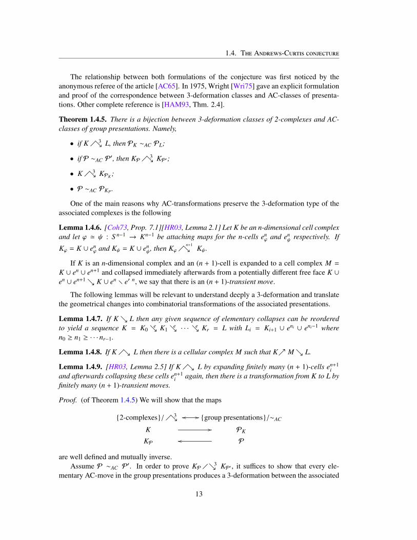
1.4. The Andrews-Curtis conjecture

The relationship between both formulations of the conjecture was first noticed by theanonymous referee of the article [AC65]. In 1975, Wright [Wri75] gave an explicit formulationand proof of the correspondence between 3-deformation classes and AC-classes of presenta-tions. Other complete reference is [HAM93, Thm. 2.4].

Theorem 1.4.5. There is a bijection between 3-deformation classes of 2-complexes and AC-classes of group presentations. Namely,

• if K �↘3 L, then PK ∼AC PL;

• if P ∼AC P′, then KP �↘3 KP′;

• K �↘3 KPK ;

• P ∼AC PKP .

One of the main reasons why AC-transformations preserve the 3-deformation type of theassociated complexes is the following

Lemma 1.4.6. [Coh73, Prop. 7.1][HR03, Lemma 2.1] Let K be an n-dimensional cell complexand let ϕ ' ψ : S n−1 → Kn−1 be attaching maps for the n-cells en

ϕ and enψ respectively. If

Kϕ = K ∪ enϕ and Kψ = K ∪ en

ψ, then Kϕ �↘n+1

Kψ.

If K is an n-dimensional complex and an (n + 1)-cell is expanded to a cell complex M =

K ∪ en ∪ en+1 and collapsed immediately afterwards from a potentially different free face K ∪en ∪ en+1↘ K ∪ en r e′ n, we say that there is an (n + 1)-transient move.

The following lemmas will be relevant to understand deeply a 3-deformation and translatethe geometrical changes into combinatorial transformations of the associated presentations.

Lemma 1.4.7. If K↘ L then any given sequence of elementary collapses can be reorderedto yield a sequence K = K0↘

e K1↘e · · · ↘e Kr = L with Li = Ki+1 ∪ eni ∪ eni−1 where

n0 ≥ n1 ≥ · · · nr−1.

Lemma 1.4.8. If K �↘ L then there is a cellular complex M such that K↗ M↘ L.

Lemma 1.4.9. [HR03, Lemma 2.5] If K �↘ L by expanding finitely many (n + 1)-cells en+1i

and afterwards collapsing these cells en+1i again, then there is a transformation from K to L by

finitely many (n + 1)-transient moves.

Proof. (of Theorem 1.4.5) We will show that the maps

{2-complexes}/�↘3 oo // {group presentations}/∼AC

K // PK

KP Poo

are well defined and mutually inverse.Assume P ∼AC P

′. In order to prove KP �↘3 KP′ , it suffices to show that every ele-mentary AC-move in the group presentations produces a 3-deformation between the associated

13

Chapter 1. Group presentations, 3-deformations and the Andrews-Curtis conjecture

2-complexes. The replacement of r j by r−1j yields attaching maps with inverse orientation.

Thus, the respective presentation complexes KP and KP′ are homeomorphic. Now, the re-placement of r j by wr jw−1 = r′j is translated in homotopic attaching maps of the 2-cells e2

j

and e′2j in KP and KP′ respectively. By Lemma 1.4.6, KP �↘3 KP′ . The replacement of r j

by r jrk = r′j yields a 3-deformation since e2k ∈ KP r {e

2j}, and then, the attaching maps of e2

j

and e′2j are homotopic. Finally, the addition of a new generator x and a new relator xw−1 withw ∈ F(x1, x2, · · · , xn) corresponds to an elementary expansion in KP; the inverse operation, toan elementary collapse.

Now, assume that K �↘3 L. By Lemmas 1.4.7 and 1.4.8, there is a deformation which canbe decomposed in the following way

K↗ K↗ M↘ L↘ L

where dim(K) = 2, dim(L) = 2, dim(M) = 3 and K↗ M↘ L are 3-dimensional expansionsand collapses.

Suppose K = K0 ↗e K1 ↗

e · · · ↗e Kr = K. Every elementary expansion of dimension1 from Ki to Ki+1 increases in one edge the spanning tree used in the construction of theassociated presentation, butPKi = PKi+1 . If Ki ↗

e Ki+1 = Ki∪e1∪e2 is an elementary expansionof dimension 2, then PKi+1 is obtained from PK1 after adding one generator x associated to e1

and one relator xw associated to e2. Thus, PKi ∼AC PKi+1 . Therefore, PK ∼AC PK . A similarreasoning shows that PL ∼AC PL.

By Lemma 1.4.9, the deformation K↗ M↘ L can be decomposed into a sequence oftransient moves. We proceed by induction. Suppose K ↗e M↘e L. That is, M = K ∪ e2 ∪ e3 =

L∪ e′2∪ e3. Notice that e2 ∈ L and e′2 ∈ K. If r is the relator in PK∪e2 associated to e2 and r′ isthe relator in PL∪e′2 associated to e′2, then it can be shown that r′ = wr±1w−1s, where s is theproduct of the relators associated to the 2-cells in ∂e3 r

(e2 ∪ e′2

)(see [HR03, Lemma 2.6]).

Thus, PK ∼AC PL. Therefore, we have proved that K �↘3 L, then PK ∼AC PL.We show now that K �↘3 KPK . If T ⊆ K1 ⊆ K is a spanning tree, then it can be shown that

K �↘3 K/T . Note that (K/T )1 is homeomorphic to KP(K). The 2-cells of each K/T and KPK

are in correspondence, differing maybe in the orientation and in the attaching maps, which arehomotopic. By Lemma 1.4.6, K/T �↘3 KPK .

Finally, to see that P ∼AC PKP , it suffices to note that the choice of orientations and atta-ching maps in KP can be done in such a way that PKP = P.

Hence, the assignments K 7→ PK andP 7→ KP induce inverse maps between 3-deformationclasses of 2-complexes and AC-classes of group presentations. �

1.5 Relationship with other open problems in low dimensionaltopology

This is the statement of the original Poincaré conjecture, which was proved by Perelman in2002 [Per02, Per03b, Per03a].

Poincaré Conjecture. Let M be a compact 3-dimensional manifold without boundary. IfM is homotopy equivalent to S 3, then M is homeomorphic to S 3.

14

1.6. Potential counterexamples

A question related with the Poincaré conjecture was formulated by Zeeman [Zee64].

Conjecture 1.5.1. (Zeeman) If K is a 2-dimensional finite contractible simplicial complex,then K × I↘ ∗.

Remark 1.5.2. Zeeman’s conjecture implies the Andrews-Curtis conjecture. In fact, if K is a2-dimensional cell complex, then there exists a simplicial complex L of dimension 2 such thatK �↘3 L (see 1.2.10). By Zeeman’s conjecture L × I↘ ∗. Therefore, K �↘3 L↗ L × I↘ ∗.Since L × I has dimension 3, we can conclude that K �↘3 ∗.

Zeeman proved that his conjecture was relevant in the study of the Poincaré conjecture.

Theorem 1.5.3. Zeeman’s conjecture implies the Poincaré conjecture.

Proof. Let M be a triangulated compact 3-dimensional manifold without boundary such thatM is homotopy equivalent to S 3. Let σ ∈ M be a 3-simplex. Consider N = Mrσ, a 3-manifoldwith boundary ∂N = ∂σ homeomorphic to S 2. On the one hand, χ(N) = χ(M) + 1 = χ(S 3) +

1 = 1. On the other hand, since N is a 3-manifold with boundary, there exists a subcomplexK ⊆ N of dimension 2 such that N↘ K. In particular, K is homotopy equivalent to N and thenπ1(K) = π1(N) = π1(M) = π1(S 3) = 0. Thus, K is simply connected and χ(K) = χ(N) = 1.Therefore, K is contractible. By Zeeman’s conjecture, K × I↘ ∗. Hence, N × I↘ K × I↘ ∗.By Whitehead’s characterization of p.l. balls (see [Coh69, RS72]) N × I is homeomorphic toD4 and N = N×{0} is contained in ∂(N× I) = N× I∪N×{0}∪N×{1}, which is homeomorphicto S 3. By the Alexander-Schoenflies Theorem (see [Moi77, Ch. I]), N is homeomorphic to D3.Therefore M = N ∪∂σ σ, which is homeomorphic to D3 ∪∂D3 D3 = S 3. �

In [GR83], Gillman and Rolfsen proved that for a class of complexes called standardspines, the Poincaré conjecture and the Zeeman conjecture are equivalent. In particular, sincethe Poincaré conjecture is true, we know that the Andrews-Curtis conjecture holds for standardspines.

1.6 Potential counterexamples

An AC-trivialization of a finite presentation P is an AC-transformation of P into the presenta-tion 〈 | 〉. No AC-trivialization is known for the following examples of balanced presentations ofthe trivial group. They are known as potential counterexamples to disprove the Andrews-Curtisconjecture.

(i) 〈x, y | xy2x−1 = y3, yx2y−1 = x3〉, Crowell & Fox (1963) [CF77, p.41].

(ii) 〈x, y, z | z−1yz = y2, x−1zx = z2, y−1xy = x2〉, Rapaport (1968) [Rap68a].

(iii) 〈x, y | x = [xm, yn], y = [xp, yq]〉, m, n, p, q ∈ Z, Gordon (1984) [Bro84].

(iv) 〈x, y | xyx = yxy, x4 = y5〉, Akbulut & Kirby (1985) [AK85].

(v) 〈x, y | x4y3 = y2x2, x6y4 = y3x3〉, M. Wicks (folklore).

15

Chapter 1. Group presentations, 3-deformations and the Andrews-Curtis conjecture

Example (i) was introduced by R. H. Crowell and R. H. Fox. It belongs to a more generalclass of presentations of the trivial group proposed by Miller and Schupp in 1999, decribed as〈x, y | xynx−1 = yn+1, x = w〉, with w a word in x and y with exponent sum 0 on x and n > 0[MS99].

Example (ii) belongs to a series of presentations with n generators xi and relators x−1i xixi+1 =

x2i . However, for n ≥ 4, the presented group is not trivial, and for n = 2, it can be easily AC-

trivialized.Example (iii) corresponds to a handle decomposition of the Akbulut-Kirby 4-sphere. It

belongs to the famous series 〈x, y | xyx = yxy, xn = yn+1〉 of presentations of the trivial group.For n = 1, it is trivially AC-trivializable. For n = 2, it was proved to be AC-trivializable in1988 by Gersten in an unpublished work. It was not until the 2000’s that Miasnikov [Mia99]and Havas and Ramsay [HR03] exhibited independently concrete AC-trivializations of thispresentation by using different computational techniques. For n > 2 there are not known AC-trivializations, despite the efforts of many authors. The presentation 〈x, y | xyx = yxy, x3 = y4〉

is the smallest potential counterexample to the Andrews-Curtis conjecture.Example (iv) was due to C. Gordon. Many of the presentations of this series are easily

AC-trivializable; for instance, those presentations in this sequence whose total relator length is10 or 12. In [BM06], Bowman and McCaul proved that all the presentations with total relatorlength equal to 14 are AC-trivializable.

1.7 Outline of the previous works on the conjecture

Classical works on the conjecture were made by Andrews and Curtis [AC66], Rapaport [Rap68b,Rap68a], Metzler and Hog-Angeloni [Met79, HAM90]. They contributed to the question ofwhether there exists some analogy between Nielsen’s or Whitehead’s algorithm for free groups(see [LS01, Ch. 1]) and the problem of finding an AC-trivialization for a given balanced pre-sentation of the trivial group. These works are focused on looking for strategies to “simplify”the presentation, where the simplification can be interpreted as a reduction of the number ofrelators, or the total length of the relators (the relator length, for short). They also found alge-braic criteria to decide weather two presentations are AC-equivalent. For a detailed expositionof these results, see [HAM93, Ch. XII].

Modern advances in the study of the conjecture were developed by means of computationaltools. In 1999, Miasnikov [Mia99] designed a genetic algorithm which proved that all balancedpresentations of the trivial group in which the relator length is at most 12 satisfy the conjec-ture. In particular, he showed that the Andrews-Curtis conjecture holds for the presentation〈x, y | xyx = yxy, x2 = y3〉, one of the potential counterexamples.

Miasnikov algorithm was non-deterministic, making a limited exploration on the searchspace. Note that an exhaustive search in the tree of AC-equivalent presentations is extremelyexpensive in memory and execution time. For instance, if the presentation has n relators thenthere are (3n2)k presentations equivalent to the original in k steps if we do not allow to in-crease/decrease the number of relators.

In 2003, Havas and Ramsay [HR03] exhibited a computational approach based on a breadth-first constrained search of the tree of equivalent presentations with bounds on the relator length.

16

1.7. Outline of the previous works on the conjecture

They implemented a software, the AC-move enumeration software (also known as ACME), toprove that if the relator length is 13 and there are two generators, all presentations of the trivialgroup are AC-equivalent to the presentation 〈x, y | x3 = y4, xyx = yxy〉.

In 2006, Bowman and McCaul [BM06] made an optimized computer program for fastsearching sequences of AC-transformations and they applied it to test the validity of the con-jecture for the potential counterexamples, which are particularly hard to reduce. The programwas again based in the breadth-first search technique, but they also added an effective use ofdisk memory and used the idea of “canonical form” of a presentation to reduce the searchspace. Despite the improvements in the implementation, they were not able to prove that〈x, y | x3 = y4, xyx = yxy〉 satisfies the conjecture. However, they showed that all the presenta-tions in the sequence due to Gordon whose total relator length is 14 are AC-trivializable.

In 2015, Bridson [Bri15] constructed explicit balanced presentations Pn of the trivial groupwith length relator at most 24(n + 1) for which the number of AC-transformations required inany trivialization grows more quickly than any tower of exponentials. Thus, it is physicallyimpossible to exhibit an explicit sequence of AC-transformations trivializing rather small ba-lanced presentations of the trivial group. While various researchers were using computer exper-iments to prove potential counterexamples to the Andrews-Curtis conjecture, he alerted to haveextreme caution when designing an experiment to find a trivializing sequence of AC-moves.

The construction of Bridson was based in groups G with presentations of deficiency 1 satis-fying certain technical conditions, which were transformed into balanced group presentationsPw indexed by words w in the generators of G such that w = 1. The groups Pw result Andrews-Curtis trivializable and the number of Andrews-Curtis transformations required to trivializethem can be bounded above and below in terms of how hard it is to prove that w = 1 in G. Inshort, he encoded the complexity of the word problem in certain groups in terms of balancedpresentations.

Summarizing, one of the most difficulties in working with finitely presented groups is thefact that a lot of problems about them are unsolvable. Even if algorithms exist, many of themare exponential or super exponential in nature, making it very unlikely for them to produceresults in an acceptable period of time. The decidability of the problem of determining if a ba-lanced presentation corresponds to the trivial group is not known. In this direction, SiddharthaGadgil [Gad01] proved that if the Andrews-Curtis conjecture were true, then there would be analgorithm to recognize balanced presentations of the trivial group.

17

Chapter 1. Group presentations, 3-deformations and the Andrews-Curtis conjecture

18

Resumen del capítulo 1: Presentaciones de grupo, 2-complejos y laconjetura de Andrews-Curtis

En este capítulo hacemos una reseña histórica del problema, desde su formulación originalhasta los avances realizados al día de hoy. Para una explicación más detallada, ver [HAM93].

En 1965, en su famoso artículo "Free groups and handlebodies" [AC65], Andrews y Curtisplantearon una pregunta sobre presentaciones de grupos, generalizando el teorema de Nielsensobre grupos libres [Nie18]. Su motivación en ese momento era la la conjetura de Poincaré.El referí (anónimo) del artículo les observa que (una versión más débil de) la conjetura está enestrecha conexión con un problema abierto sobre deformaciones de CW-complejos.

Conjetura 1.4.3 (Andrews-Curtis). Si P = 〈x1, · · · , xn | r1, · · · , rn〉 es una presentación bal-anceada del grupo trivial, entonces P se puede llevar a la presentación vacía 〈 | 〉 medianteuna sucesión finita de las siguientes transformaciones:

• reemplazar ri por r−1i ,

• reemplazar ri por rir j, j , i,

• reemplazar ri por wriw−1, donde w es una palabra en los generadores,

• agregar un nuevo generador x y la relación x, o el inverso de esta operación.

La relación notada por el referí entre presentaciones grupos y CW-complejos de dimensión2 fue recién formalizada y probada por Wright [Wri75].

Definición 1.3.1. Sea K un complejo celular de dimensión 2. La presentación de grupo están-dar PK asociada a K es la presentación definida como sigue.

• Elegir e0 ∈ K0 una 0-celda de K como punto base.

• Elegir T ⊆ K1 un spanning tree (i.e., un subcomplejo contráctil de su 1-esqueleto quecontenga todos los vértices).

• Sean e11, e

22 · · · , e

1n las 1-celdas de in K r T . Para cada 1 ≤ i ≤ n, elegir una orientación

para e1i , y sea xi el único camino en T desde e0 al inicio de e1

i seguido por e1i y luego

por el camino desde su final a e0. Entonces, xi ∈ π1(K1, e0) y, más aún, π1(K1, e0) =

F(x1, x2, · · · , xn).

• Sean e21, e

22, · · · , e

2m las 2-celdas de K. Para cada e2

j , elegir una función de adjunción ϕ j,un punto base s0 y una orientación ∂D2. Luego, ϕ j es un ciclo en ϕ j(s0).

• Para cada 1 ≤ j ≤ m, elegir un camino γ j in K1 desde e0 a ϕ j(s0) y considerar el cicloγ j ∗ ϕ j ∗ γ j. Luego, [γ j ∗ ϕ j ∗ γ j] ∈ π1(K1, e0), y puede expresarse como un producto r j

de los elementos {x1, x2, · · · , xn} y sus inversos.

• Definir PK = 〈x1, x2, · · · , xn | r1, r2, · · · , rm〉.

19

Capitulo 1: Presentaciones de grupo, 2-complejos y la conjetura de Andrews-Curtis

Definición 1.3.7. Sea P = 〈x1, x2 · · · , xn | r1.x2, · · · , rm〉 una presentación de grupo finita. Elcomplejo de presentación KP es el complejo celular construido como sigue:

• su 0-esqueleto es un único punto;

• para cada generador xi, adjuntar a la 0-celda una 1-celda orientada e1i , obteniendo un

bouquet de círculos∨n

i=1 S 1;

• cada relación r j determina un camino cerrado ϕ j en∨n

i=1 S 1; para cada 1 ≤ j ≤ madjuntar una 2-celda e2

j con función de adjunción ϕ j.

Teorema 1.4.5. Hay una correspondencia entre clases de 3-deformación de 2-complejos yclases de Andrews-Curtis de presentaciones de grupos. Concretamente

• si K �↘3 L, entonces PK ∼AC PL;

• si P ∼AC P′, entonces KP �↘3 KP′ ;

• K �↘3 KPK ;

• P ∼AC PKP .

Luego, la conjetura de Andrews-Cutis se puede reformular en términos topológicos delsiguiente modo.

Conjetura 1.2.9 (Conjetura de Andrews-Curtis, versión topológica). Si K es un 2-complejocontráctil, entonces K �↘3 ∗.

Ambas versiones de la conjetura fueron ampliamente estudiadas, obteniéndose hasta ahoraresultados parciales. Por ejemplo, se sabe que la conjetura es cierta para ciertas clases decomplejos, como los standar spines y los complejos cuasi-construibles.

Hay una lista de presentaciones balanceadas del grupo trivial ampliamente estudiada paralas cuales no se conoce ninguna lista de movimientos de Andrews-Curtis que las lleven a lapresentación vacía. Son potenciales contraejemplos para refutar la conjetura.

(i) 〈x, y | xy2x−1 = y3, yx2y−1 = x3〉, Crowell & Fox (1963) [CF77, p.41].

(ii) 〈x, y, z | z−1yz = y2, x−1zx = z2, y−1xy = x2〉, Rapaport (1968) [Rap68a].

(iii) 〈x, y | x = [xm, yn], y = [xp, yq]〉, m, n, p, q ∈ Z, Gordon (1984) [Bro84].

(iv) 〈x, y | xyx = yxy, xn = yn+1〉, n ≥ 3, Akbulut & Kirby (1985) [AK85].

En los próximos capítulos desarrollaremos métodos para abordar ambas versiones de laconjetura así como también la lista de de potenciales contraejemplos, con técnicas de espaciostopológicos finitos.

20

Chapter 2

The finite spaces point of view

The theory of finite spaces can be used to study homotopy properties of more general spaces.In fact, finite spaces model the weak homotopy types of compact polyhedra. In this chapter wewill recall the basic results and constructions about this theory.

2.1 Algebraic topology of finite spaces

The theory of finite spaces started in 1937 by P. S. Alexandroff [Ale37], who showed that theyhave an intrinsic combinatorial structure: they can be thought of as finite partially ordered sets(posets). In 1966, M. C. McCord [McC66] made a great advance in the theory establishing thecorrespondence of weak homotopy types between compact cell complexes and finite spaces.The same year, R. E. Stong [Sto66] proved that the homotopy type of finite spaces can bealgorithmically decided by a simple reduction procedure of low complexity. More recently, J.A. Barmak and E. G. Minian studied different algebraic topology problems using the interactionbetween topology and combinatorics. Among other contributions, they developed the simplehomotopy theory of finite spaces, and applied methods of finite spaces to the study of theAndrews-Curtis conjecture [Bar11a].

2.1.1 Finite spaces and posets

In 1937, Alexandroff [Ale37] proved that finite T0-spaces and finite posets are basically thesame object viewed from different perspectives. Given a finite topological space X, define arelation ≤ in X by x ≤ y if x ∈ Uy, where Uy is the minimal open set containing y. It is clearthat ≤ is reflexive and transitive. If X is T0, ≤ is also antisymmetric. Conversely, if ≤ is areflexive and transitive relation on X the sets

{Ux

}x∈X where Ux =

{y ∈ X : y ≤ x

}, constitute

a basis for a topology on X. If ≤ is antisymetric, the topology defined on X will additionallysatisfy the T0-axiom. From now on, all finite spaces will be assumed to be T0 and we will referindistinctly to both structures, the topological one and the combinatorial one.

Note that a map f : X → Y between finite spaces is continuous if and only if it is anorder-preserving map.

A poset X can be represented as a directed graph, its Hasse diagram, denoted byH(X). Its

21

Chapter 2. The finite spaces point of view

vertices are the elements of X, and its edges are the pairs (x, y) such that x ≺ y, i.e., x < y andthere is no z ∈ X satisfying x < z < y.

A chain in a finite poset X is a totally ordered subset c = {x0 < x1 < · · · < xn} of X. Thelength of the chain c is n.

The height h(X) of a finite poset X is the maximum length of a chain of X. The height of apoint x ∈ X is hX(x) = h(Ux).

Figure 2.1: Hasse diagrams of some finite topological spaces.

2.1.2 Finite spaces and cellular complexes

Although general Hausdorff spaces do not have the homotopy type of a finite space, McCordproved in 1966 [McC66] that every finite cellular complex has an associated finite space withthe same weak homotopy type.

Definition 2.1.1. There is a functor K : Top<∞ → S from the category of finite spaces to thecategory of finite complexes defined by:

• if X is a finite space, K(X) is the order complex of X, that is, the simplicial complexwhose simplices are the nonempty chains of X;

• if f : X → Y is a continuous map between finite spaces, K( f ) : K(X) → K(Y) is thesimplicial map defined by K( f )(x) = f (x).

22

2.1. Algebraic topology of finite spaces

Figure 2.2: Order complexes of some finite topological spaces.

Notice that not every finite simplicial complex is the order complex of a finite space. Somenecessary conditions are that K must be a clique complex and its 1-skeleton must be a compa-rability graph. Recall that a complex is a clique complex if its simplices are exactly the cliquesof the graph induced by its 1-skeleton. An undirected graph is a comparability graph if thereexists a transitive orientation of its edges, that is, an assignment of directions to its edges suchthat for every pair (x, y), (y, z) of oriented edges, there exists a directed edge (x, z). This classof graphs is completely described by forbidden subgraphs: a graph is of comparability if andonly if it does not contain cycles of odd length n ≥ 5 as induced subgraphs. We prove that theprevious conditions are sufficient to characterize order complexes.

Proposition 2.1.2. A finite simplicial complex K is the order complex of some finite space ifand only if its simplices are the cliques on its 1-skeleton, and its 1-skeleton does not containodd cycles of length greater than 3.

Proof. Assume K = K(X) for a finite space X. The vertices of K coincide with the underlyingset of X and the simplices of K are the nonempty chains of X. Non empty chains of X corre-sponds with cliques in K1. Thus, K is a clique complex. The order in X induces a transitiveorientation of the edges of K1. Thus, K1 is a comparability graph.

Conversely, if K1 is a comparability graph, then consider a transitive orientation on itsedges. The orientation induces an acyclic order ≤ of its vertices K0. Let X be the finite spaceassociated with the poset (K0,≤). Since K is clique complex, K = K(X). �

23

Chapter 2. The finite spaces point of view

Recall that a CW-complex K is regular if for every open cell en, the attaching map Dn → Kof its cells en is a homeomorphism.

Definition 2.1.3. There is a functor X : CWreg → Top<∞ from the category of finite regularcell complexes to the category of finite spaces, defined by:

• if K is a finite regular cell complex X(K) is the face poset of K, that is, the finite spacewhose underlying set is the set of all cells of K with the order-relation e < e′ if e is a faceof e′;

• if f : K → L is a cellular map between finite regular cell complexes, thenX( f ) : X(K)→X(L) is the continuous map defined by X( f )(e) = f (e).

Figure 2.3: Face posets of some regular cell complexes.

24

2.1. Algebraic topology of finite spaces

Remark 2.1.4. The functors K and X are not mutually inverse. Given a finite regular cellcomplex K, the composition K(X(K)) is the barycentric cell subdivision K′ of K, i.e. thesimplicial complex whose vertices are the cells of K and {e1, e2, · · · , en+1} is an n-simplex ifei is a face of ei+1 for each i. Conversely, if X is a finite space, then X(K(X)) is the so calledbarycentric poset subdivision X′ of X, which is the poset of chains of X ordered by inclusion.

Definition 2.1.5. There are natural transformations:

• µX : |K(X)| → X, defined by µX(α) = min(support(α)), where the support of a convexcombination α =

∑ri=1 tixi of the vertices of K(X) is understood to be the set of vertices

accompanied by a nonzero coefficient,

• µK : |K| → X(K), µK = µX(K)s−1K , where sk : |K′| → |K| is the linear homemorphism

defined by sK(e) = b(e), the barycenter of e.

Recall that a continuous map f : X → Y between topological spaces is said to be a weakhomotopy equivalence if it induces isomorphisms in all homotopy groups. McCord proved thatthe previous maps are weak equivalences.

Theorem 2.1.6. [McC66] µX and µK are natural weak homotopy equivalences. In particular,

• a map f : X → Y between finite T0-spaces is a weak equivalence if and only if K( f ) :K(X)→ K(Y) is a homotopy equivalence.

• a map f : K → L between finite regular cell complexes is a homotopy equivalence if andonly if X( f ) : X(K)→ X(L) is a weak equivalence.

Remark 2.1.7. In [Bar11a, Thm. 11.3.2.], Barmak gave an alternative proof of the fact thatX(K) and K are weak equivalent. He defined the map

νK : K → X(K)op

as νK(x) = e if x ∈ e. He uses the same ideas of McCord to prove that νK is a weak equivalence.

Homotopy equivalences are weak homotopy equivalences and, in the category of cellularcomplexes weak homotopy equivalences are homotopy equivalences, by the Whitehead Theo-rem [Hat02, Thm. 4,5]. We will see in Section 2.1.3 that both notions do not coincide in thecategory of finite spaces.

We can deduce Theorem the following consequence of Theorem 2.1.6.

Corollary 2.1.8. If K is a regular cell complex, then K is contractible if and only if X(K) ishomotopically trivial. If X is a finite space, then X is homotopically trivial if and only if K(X)is contractible.

McCord’s result is supported on the following Theorem, which gives a criterion for recog-nizing weak homotopy equivalences between topological spaces.

An open coverU of a topological space X is called a basis like open cover ifU is a basisfor some topology in the underlying set of X (possibly different from the original one).

25

Chapter 2. The finite spaces point of view

Theorem 2.1.9. (McCord) [McC66, Thm 6] Let X and Y be topological spaces and let f :X → Y be a continuous map. If there exists a basis like open cover U of Y such that eachrestriction f | f −1(U) : f −1(U)→ U is a weak equivalence for every U ∈ U, then f : X → Y is aweak equivalence.

In the same line, the celebrated Theorem A of Quillen [Qui72] provides a sufficient con-dition for a functor to induce a homotopy equivalence between the classifying spaces of theinvolved categories. Quillen’s Theorem A applied to the case when both categories are finiteposets coincides with McCord’s Theorem applied to the minimal basis coverU = {Uy : y ∈ Y},and can be summarized in the following result.

Theorem 2.1.10. (Quillen’s Fiber Lemma)[Qui78, Prop. 1.6] Let f : X → Y be an orderpreserving map between finite posets such that f −1(Uy) is homotopically trivial for every y ∈ Y.Then f : X → Y is a weak equivalence.

Barmak exposed a simpler proof of the previous statement using the notion of non-Hausdorffmapping cylinder (see Proposition 3.0.1 below and [Bar11b, Thm. 1.1, 1.2]).

2.1.3 Homotopy types

The homotopy type of finite spaces can be classified combinatorially by means of a method ofreduction: the beat points. This description was discovered in 1966 by Stong [Sto66].

Recall that, given a finite space X and x ∈ X, we denote by UXx the minimal open set

containing x, i.e., UXx = {y ∈ X : y ≤ X}. Similarly, FX

x denotes the closure of x in X, that is,FX

x = {y ∈ X : x ≤ y}. We omit the superscript when the poset is understood.

Definition 2.1.11. Let X be a finite space. An element x ∈ X is called an up beat point ifthere is a unique element y ∈ X such that x ≺ y, i.e., the set Fx = Fx r {x} has a minimum.Analogously x is called a down beat point if there is a unique y such that y ≺ x, i.e., the setUx = Ux r {x} has maximum. In both cases we say that x is a beat point dominated by y.

If x ∈ X is a beat point, then X r {x} is a strong deformation retract of X. We denote it byX↘↘ X r {x}. In general we denote X↘↘ Y if there is a sequence X = X0, . . . , Xn = Y such thatXi is obtained from Xi−1 by removing a beat point. Note that in this case, Y ⊆ X is a strongdeformation retract.

A core of a finite T0-space X is a strong deformation retract of X without beat points.

The following result was proved by Stong [Sto66] (see also [Bar11a]).

Theorem 2.1.12. The core of a finite space is unique up to homeomorphism and two finitespaces are homotopy equivalent if and only if the have homeomorphic cores. In particular, afinite space is contractible if and only if its core is a singleton.

As consequence, it can be deduced that finite spaces with maximum or minimum are con-tractible. Indeed, if X has a maximum x, then the maximal points of X r {x} are up beat points,so we can remove them and iterate. Thus, the core of X is homeomorphic to {x}. An analogousprocedure works for spaces with minimum.

26

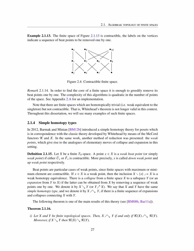
2.1. Algebraic topology of finite spaces

Example 2.1.13. The finite space of Figure 2.1.13 is contractible, the labels on the verticesindicate a sequence of beat points to be removed one by one.

•4 •9 •10

•1 •3 •6 •8

•2 •5 •7 •

Figure 2.4: Contractible finite space.

Remark 2.1.14. In order to find the core of a finite space it is enough to greedily remove itsbeat points one by one. The complexity of this algorithms is quadratic in the number of pointsof the space. See Appendix 2.A for an implementation.

Note that there are finite spaces which are homotopically trivial (i.e. weak equivalent to thesingleton) but not contractible. That is, Whitehead’s theorem is not longer valid in this context.Throughout this dissertation, we will see many examples of such finite spaces.

2.1.4 Simple homotopy types

In 2012, Barmak and Minian [BM12b] introduced a simple homotopy theory for posets whichis in correspondence with the classic theory developed by Whitehead by means of the McCordfunctors K and X. In the same work, another method of reduction was presented: the weakpoints, which give rise to the analogues of elementary moves of collapse and expansion in thissetting.

Definition 2.1.15. Let X be a finite T0-space. A point x ∈ X is a weak beat point (or simplyweak point) if either Ux or Fx is contractible. More precisely, x is called down weak point andup weak point respectively.

Beat points are particular cases of weak points, since finite spaces with maximum or mini-mum element are contractible. If x ∈ X is a weak point, then the inclusion X r {x} ↪→ X is aweak homotopy equivalence. There is a collapse from a finite space X to a subspace Y (or anexpansion from Y to X) if the latter can be obtained from X by removing a sequence of weakpoints one by one. We denote it by X↘ Y (or Y↗ X). We say that X and Y have the samesimple homotopy type, and we denote it by X �↘ Y , if there is a finite sequence of expansionsand collapses connecting X with Y .

The following theorem is one of the main results of this theory (see [BM08b, Bar11a]).

Theorem 2.1.16.

i) Let X and Y be finite topological spaces. Then, X �↘ Y if and only if K(X)�↘ K(Y).Moreover, if X↘ Y then K(X)↘ K(Y).

27

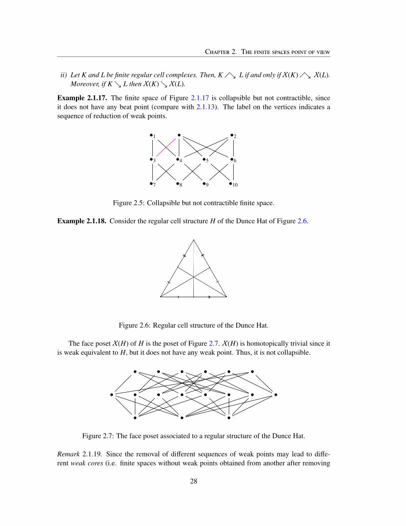
Chapter 2. The finite spaces point of view

ii) Let K and L be finite regular cell complexes. Then, K �↘ L if and only ifX(K)�↘ X(L).Moreover, if K↘ L then X(K)↘ X(L).

Example 2.1.17. The finite space of Figure 2.1.17 is collapsible but not contractible, sinceit does not have any beat point (compare with 2.1.13). The label on the vertices indicates asequence of reduction of weak points.

•1 • •2

•3 •4 •5 •6

•7 •8 •9 •10

Figure 2.5: Collapsible but not contractible finite space.

Example 2.1.18. Consider the regular cell structure H of the Dunce Hat of Figure 2.6.

Figure 2.6: Regular cell structure of the Dunce Hat.

The face poset X(H) of H is the poset of Figure 2.7. X(H) is homotopically trivial since itis weak equivalent to H, but it does not have any weak point. Thus, it is not collapsible.

• • • • • •

• • • • • • • •

• • •

Figure 2.7: The face poset associated to a regular structure of the Dunce Hat.

Remark 2.1.19. Since the removal of different sequences of weak points may lead to diffe-rent weak cores (i.e. finite spaces without weak points obtained from another after removing

28

2.2. The Andrews-Curtis conjecture in the context of finite spaces

successively weak points), an exhausted exploration of all possible sequences of reductions isnecessary to find the weak core with minimum cardinality. A backtracking algorithm to exploreall possible sequences of collapses is implemented in 2.A. Memorization of already exploredspaces and pruning criteria is used to optimize the complexity, which is a priori the factorial ofthe number of points of the space.

Remark 2.1.20. If Ux or Fx is contractible, then X↘ X r {x}. Thus, by Theorem 2.1.16,K(X)↘ K(X r {x}). Less restrictive conditions can be considered to obtain similar results:

• If Ux or Fx is collapsible, then K(X)↘ K(X r {x}). Such points x were studied in[BM12b] when investigating non-evasiveness and strong collapsibility from the finitespaces point of view.

• If Ux or Fx is homotopically trivial, then K(X)�↘ K(X r {x}). Such points x arecalled γ-points and were defined in [BM08a] when studying different one-point reductionmethods.

• If Ux or Fx is acyclic, thenHi(K(X)) � Hi(K(Xr {x})) for all i. Such points x were alsointroduced in [BM08a]; we will refer to them as acyclic points.

• If Ux or Fx is n-connected (i.e. πi(Ux) � 0 for all 1 ≤ i ≤ n), then X r {x} → X isan (n + 1)-equivalence (i.e. it induces an isomorphism πi(X r {x}, x0) → π1(X, x0) fori < n + 1 and an epimorphism for i = n). The proof of the previous fact can be found in[Bar11b, Lemma 6.2.].

2.2 The Andrews-Curtis conjecture in the context of finite spaces

The development of the simple homotopy theory of finite spaces allows one to reformulate theAndrews-Curtis conjecture in this context.

Definition 2.2.1. Let X and Y be two finite topological spaces. We say that X n-deforms to Y ,and we denote it by X �↘n Y , if Y can be obtained from X by performing a finite sequence ofexpansions and collapses in such a way that all the spaces involved are of height at most n.

The Andrews-Curtis Conjecture can be reformulates as follows.

Conjecture 2.2.2. Let X be a homotopically trivial finite space of height 2. Then X 3-deformsto a point.

The following result is well-known. See for example [Whi39, HAM93].

Lemma 2.2.3. Let K be a regular n-dimensional cell complex and K′ = K(X(K)) the barycen-tric subdivision of K. Then, K �↘

n+1K′.

In the context of finite spaces we have the following similar result.

Lemma 2.2.4. [Bar11a, Prop. 4.2.9.] Let X be a finite T0-space of height n and let X′ =

X(K(X)) be the subdivision of X. Then, X �↘n+1

X′.

29

Chapter 2. The finite spaces point of view

Theorem 2.2.5. Conjecture 2.2.2 is equivalent to the Andrews–Curtis conjecture.

Proof. Assume Conjecture 2.2.2 holds. If K is a contractible regular 2-complex, then X(K) isa homotopically trivial finite space of height 2. Hence, X(K)�↘3 ∗. Then, as a consequence ofTheorem 2.1.16, K′ �↘3 ∗. Finally, Lemma 2.2.3 implies that K �↘3 ∗. Conversely, supposethat the Andrews-Curtis conjecture is true and let X be a homotopically trivial finite space ofheight 2. Then K(X) is contractible and by the hypothesis K(X)�↘3 ∗. This implies thatX′ �↘3 ∗. Since X �↘3 X′ by Lemma 2.2.4, the result follows. �

In [Bar11a, Ch.11] Barmak described a class of simplicial complexes, the quasi-constructiblecomplexes, which satisfy the Andrews-Curtis conjecture. The definition of these complexes issupported in a class of homotopically trivial finite spaces of height 2: the qc-reducible spaces.Concretely, quasi-constructible complexes are the order complexes of qc-reducible spaces. Thedefinition of the latter class is based in a new method of reduction of finite spaces, called qc-reduction.

Definition 2.2.6. Let X be a finite space of height at most 2. Let x, y ∈ X be two maximalelements such that Ux ∪Uy is contractible. Then, there is a qc-reduction from X to the quotientspace X/{x, y}. X is qc-reducible if after performing a sequence of qc-reductions starting fromX, one can obtain a space with maximum.

Note that if there is a qc-reduction from X to X/{x, y}, then X �↘3 X/{x, y}. In fact, X↗ X∪{z} with Uz = Ux ∪ Uy, and X ∪ {z}↘ X ∪ {z} r {x, y} since x and y are up beat points. Thelatter space is isomorphic to X/{x, y}. In particular, qc-reducible spaces 3-deform to a point.The quasi constructible spaces are the contractible simplicial complexes whose face posets areqc-reducible.

For instance, in the Dunce Hat’s Example 2.1.18, one can perform the following sequenceof qc-reductions in X(H): X(H) qc-reduces to X(H)/{x1, y1} = Y , and the last one qc-reducesto Y/{x2, y2} (see Figure 2.2). The latter space is collapsible. Thus, X(H)�↘3 ∗.

•x1 •x2 •y2 • • •y1

• • • • • • • •

• • •

Figure 2.8: Qc-reductions in the face poset of the Dunce Hat.

In Chapter 3 we develop new methods of reduction and algorithms to decide (non-exhaustively)whether a finite space of height 2 satisfies Conjecture 2.2.2. In Chapter 6 we present two newmethods to obtain presentations AC-equivalent to a given presentation of the trivial group andwe implement both (non-deterministic) algorithms to decide if it satisfies Conjecture 1.2.9. Weanticipate some examples to show the reach of the theory.

30

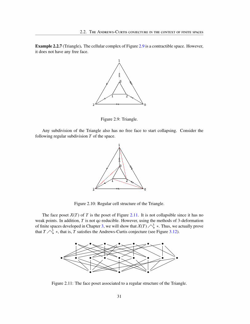
2.2. The Andrews-Curtis conjecture in the context of finite spaces

Example 2.2.7 (Triangle). The cellular complex of Figure 2.9 is a contractible space. However,it does not have any free face.

Figure 2.9: Triangle.

Any subdivision of the Triangle also has no free face to start collapsing. Consider thefollowing regular subdivision T of the space.

Figure 2.10: Regular cell structure of the Triangle.

The face poset X(T ) of T is the poset of Figure 2.11. It is not collapsible since it has noweak points. In addition, T is not qc-reducible. However, using the methods of 3-deformationof finite spaces developed in Chapter 3, we will show thatX(T )�↘3 ∗. Thus, we actually provethat T �↘3 ∗, that is, T satisfies the Andrews-Curtis conjecture (see Figure 3.12).

• • • • • • •

• • • • • • • • •

• • •

Figure 2.11: The face poset associated to a regular structure of the Triangle.

31

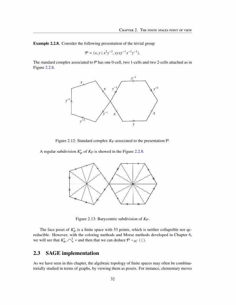
Chapter 2. The finite spaces point of view

Example 2.2.8. Consider the following presentation of the trivial group

P = 〈x, y | x2y−3, xyxy−1x−1y−1〉.

The standard complex associated to P has one 0-cell, two 1-cells and two 2-cells attached as inFigure 2.2.8.

Figure 2.12: Standard complex KP associated to the presentation P.

A regular subdivision K′P

of KP is showed in the Figure 2.2.8.

Figure 2.13: Barycentric subdivision of KP.

The face poset of K′P

is a finite space with 53 points, which is neither collapsible nor qc-reducible. However, with the coloring methods and Morse methods developed in Chapter 6,we will see that K′

P�↘3 ∗ and then that we can deduce P ∼AC 〈 | 〉.

2.3 SAGE implementation

As we have seen in this chapter, the algebraic topology of finite spaces may often be combina-torially studied in terms of graphs, by viewing them as posets. For instance, elementary moves

32

2.3. SAGE implementation

of finite spaces can be conveniently expressed in terms of algorithmic graph theory. This moti-vated us to undertake a computational approach of the previous methods. We employed the freesoftware SAGE [S+17]. In the Appendix 2.A of this chapter we include the implementationsof some basic operations on posets; most of them can be also found in [Fer11].

33

Chapter 2. The finite spaces point of view

34

2.A. Appendix: Finite spaces SAGE module

2.A Appendix: Finite spaces SAGE module

Generalities1 #Opposite of a finite space2 def op(X):3 elms = X.list()4 rels = [r[::-1 ] for r in X.cover_relations()]5 return Poset((elms,rels))6

7 #Join8 def join (X, Y):9 return X.ordinal_sum(Y)

10

11 #Cartesian Product12 def cartesian_product (X, Y):13 return X.product(Y)14

15 #Quotient16 def quotient_poset(X, A): #X poset, A the list of elements of the

subposet17 open_A = X.order_ideal(A)18 closed_A = X.order_filter(A)19 if set(open_A).intersection(closed_A) != set(A):20 return ’ERROR: X/A is not T_0’21 notinA = [x for x in X.list() if not x in A]22 elms = notinA + [A[0]]23 rels=[[x, y] for x in notinA for y in notinA if X.covers(x, y)]

+ [[A[0], x] for a in A for x in notinA if X.covers(a, x)] + [[x,A[0]] for a in A for x in notinA if X.covers(x, a)]

24 return Poset((elms, rels))25

26 #Wedge27 def wedge(X, Y, x, y):28 return quotient_poset(X.disjoint_union(Y), [x, y])

Homology1 #Homology of a finite space2 def homology(X):3 return X.order_complex().homology()

Fundamental group1 #Presentation of the fundamental group of a finite space2 def fundamental_group(X):3 return X.order_complex().fundamental_group()

35

Chapter 2. The finite spaces point of view

Closed sets, open sets, links and stars.

1 def F(X, x):2 return X.subposet(X.order_filter([x]))3

4 def U(X, x):5 return X.subposet(X.order_ideal([x]))6

7 def C(X, x):8 elms=[y for y in X.list() if X.is_gequal(x,y) or X.is_gequal(y,

x)]9 return X.subposet(elms)

10

11 def F_hat(X, x):12 elms=[y for y in X.list() if X.is_greater_than(y, x)]13 return X.subposet(elms)14

15 def U_hat(X, x):16 elms=[y for y in X.list() if X.is_greater_than(x, y)]17 return X.subposet(elms)18

19 def C_hat(X,x):20 elms=[y for y in X.list() if X.is_greater_than(x, y) or X.

is_greater_than(y, x)]21 return X.subposet(elms)

Reduction of posets

1 #remove the point x from the poset X2 def remove_point(X, x):3 elms=[y for y in X.list() if not y == x]4 return X.subposet(elms)5

6 #remove the edge x from the poset X7 def remove_edge(X, e): #e=[e[0], e[1]]8 rels=[edge for edge in X.cover_relations() if not edge == e]9 return Poset((X.list(), rels))

Homotopy Theory

1 def is_beat_point(X, x):2 return len(X.upper_covers(x)) == 1 or len(X.lower_covers(x)) ==

13

4 def beat_points(X):5 return [x for x in X.list() if is_beat_point(X,x)]6

7 def core(X):

36

2.A. Appendix: Finite spaces SAGE module

8 for x in beat_points(X):9 X = remove_point(X, x)

10 return core(X)11 return X12

13 def is_contractible(X):14 if X.has_top() or X.has_bottom():15 return True16 return core(X).cardinality() == 1

Simple Homotopy Theory1 def is_weak_point(X, x):2 return (is_contractible(U_hat(X, x)) or is_contractible(F_hat(X,

x)))3

4 def weak_points(X):5 return [x for x in X.list() if is_weak_point(X, x)]6

7 def weak_core(X):8 for x in weak_points(X):9 X = remove_point(X, x)

10 return weak_core(X)11 return X12

13 def minwcoreaux(X):14 MX = X15 for x in weak_points(X):16 S = remove_point(X, x)17 K = tuple(S.list())18 if not visitados.has_key(K):19 visitados[K] = True20 Y = minwcoreaux(S)21 if Y.cardinality()< MX.cardinality(): MX = Y22 return MX23

24 def min_weak_core(X):25 global visitados26 visitados = {}27 return minwcoreaux(X)28

29 def is_collapsible_aux(X):30 if is_contractible(X):31 return True32 if non_collapsibles.has_key(tuple(X.list())):33 return False34 for x in weak_points(X):35 S = remove_point(X,x)36 if not non_collapsibles.has_key(tuple(S.list())):

37

Chapter 2. The finite spaces point of view

37 if is_collapsible(S):38 return True39 non_collapsibles[tuple(S.list())] = True40 return False41

42 def is_collapsible(X):43 global non_collapsibles44 non_collapsibles = {}45 return is_collapsible_aux(X)

Qc-reductions

1 def is_qc_reduction(X, a, b):2 return is_contractible(X.subposet(X.order_ideal([a, b])))3

4 def is_qc_op_reduction(X, a, b):5 return is_contractible(X.subposet(X.order_filter([a, b])))6

7 #The qc-irreducible poset obtained from X by performing qc-reductions

8 def qc_core(X):9 if len(X.maximal_elements()) == 1:

10 return X11 for a in X.maximal_elements():12 for b in X.maximal_elements():13 if a != b and is_qc_reduction(X, a, b):14 X=quotient_poset(X, [a, b])15 return qc_core(X)16 return X

38

Resumen del capítulo 2: El punto de vista de los espacios finitos

En este capítulo repasamos la teoría de espacios topológicos finitos, que será una herramientafundamental en el presente trabajo. Mostramos también la reformulación de la conjetura desdeeste punto de vista. Para un desarrollo detallado de la teoría de espacios finitos, referimos allector a [Bar11a].

Los espacios topológicos finitos T0 y los conjuntos parcialmente ordenados son esencial-mente el mismo objetos desde distintas perspectivas. Dado X un espacio topológico finito,definimos la relación ≤ en X por x ≤ y si x si x pertenece al abierto minimal que contienea y. Es claro que ≤ es reflexiva y transitiva. Si X es T0, entonces ≤ es además antisimétrica.Recíprocamente, si ≤ es una relación reflexiva y transitiva en X, los conjuntos

{Ux

}x∈X , con

Ux ={y ∈ X : y ≤ x

}, son una base para una topología en X. Si ≤ es antisimética, la topología

definida en X satisfará además el axiona T0.De ahora en más, todos los espacios finitos se asumirán T0, y nos referiremos indistinta-

mente a ambas estructuras, la topológica y la combinatoria.

Los espacios finitos sirven como modelos topológicos simples para poliedros compactos.Se define un funtor K : Top<∞ → S de la categoría de espacios finitos a la categoría de

complejos simpliciales. El order complex K(X) asociado a un espacio finito X es el complejosimplicial cuyos vértices son los elementos de X y cuyos símplices son las cadenas de ele-mentos de X. Recíprocamente, se define el funtor X : CWreg → Top<∞ desde la categoría deCW-complejos regulares. El face poset X(K) de un complejo regular K es el poset de celdas deK ordenadas por inclusión.

McCord probó en [McC66] que todo complejo celular regular es débilmente equivalente aX(K). Análogamente, dado un espacio finito X, hay una equivalencia débil entre X y K(X).

Figura 2.14: Order complex asociado a algunos espacios topológicos finitos.

39

Capitulo 2: El punto de vista de los espacios finitos

Figura 2.15: Face poset asociado a algunos complejos celulares regulares.

A diferencia de lo que ocurre en la categoría de CW-complejos, el tipo homotópico (fuerte)y el tipo homotópico débil difieren en la categoría de espacios finitos.

En [Sto66], Stong mostró que el tipo homotópico de espacios finitos puede describirse demanera muy simple a partir de un movimiento básico de reducción: remover beat points. Unpunto x ∈ X es un beat point si cubre o es cubierto por un único elemento de X. El core deun espacio finito es el espacio que se obtiene a partir de X luego de remover sucesivamentesus beat points hasta llegar a un espacio irreducible. Dos espacios finitos son homotópicamenteequivalentes si y sólo si sus cores son isomorfos. En particular, un espacio finito es contráctilsi su core es un punto.

En [BM08b], Barmak y Minian desarrollan la teoría de homotopía simple para espaciosfinitos. La construyen sobre la base de un movimiento elemental: quitar y agregar weak points.Decimos que dos espacios finitos tienen el mismo tipo homotópico simple si se puede llegarde uno a otro agregando y quitando una cantidad finita de weak points. El siguiente resultadomuestra que la teoría de homotopía simple para espacios finitos modela la teoría homónima

40

para CW-complejos.

Teorema 2.1.16. i) Sean X e Y espacios topológicos finitos. Entonces, X �↘ Y si y sólo siK(X)�↘ K(Y). Más aún, si X↘ Y entonces K(X)↘ K(Y).

ii) Sean K y L complejos celulares regulares. Entonces, K �↘ L si y sólo si X(K)�↘ X(L).Más aún, si K↘ L entonces X(K)↘ X(L).

Decimos que un espacio finito X se n-deforma en Y , y lo denotamos por X �↘n Y , si Y sepuede obtener a partir de X agregando y quitando weak points, de modo que todos los espaciosinvolucrados tengan altura a lo sumo n.

La conjetura de Andrews-Curtis tiene una formulación equivalente en el contexto de espa-cios finitos.

Conjetura 2.2.2 (Conjetura de Andrews-Curtis, versión para espacios finitos). Sea X un es-pacio topológico finito homotópicamente trivial de altura 2. Entonces X se 3-deforma a unpunto.

41

Capitulo 2: El punto de vista de los espacios finitos

42

Chapter 3

3-deformation methods for finitespaces

The most natural way to relate the topology of two spaces is through continuous maps. Ma-pping cylinders embody this kind of connection in the shape of another topological space, athird one that encodes the homotopy type of the codomain and, under certain conditions overthe map, also encodes the homotopy information of the domain.

Recall that the mapping cylinder of a map f : X → Y between topological spaces is thequotient space M f := (X × I) t Y/(x,1)∼ f (x).

Both X and Y are subspaces of M f , with i : X ↪→ M f and j : Y ↪→ M f the canonicalinclusions. Moreover, Y is a strong deformation retract of M f with a retraction r : M f → Ywhich also satisfies ri = f . Then, f can be factorized as a composition of an inclusion (in fact,i is a cofibration) and a homotopy equivalence. In particular, f is a homotopy equivalence ifand only if the inclusion i is.

Xf //� _

i��

Y

M f

r

>>

Mapping cylinders are very useful homotopical tools. They have shown to be highly suit-able to reduce many proofs concerning homotopy classes of maps f : X → Y to the case

43

Chapter 3. 3-deformation methods for finite spaces

of good pairs (Y, X) (a cofibrant replacement). For example, Wall’s finiteness obstruction[Wal65, Wal66a] is an algebraic K-theory invariant which establishes if a finitely dominatedspace is homotopy equivalent to a finite CW complex. A finite domination of a space X is aCW complex K with maps d : K → X, s : X :→ K such that ds ' idX . The very first step todeal with this problem is to assume that d is an inclusion by replacing X, if necessary, by Md.This reduces the problem to the study of the relative homotopy groups associated to the pair(K, X). A construction due to Milnor [Mil59] allows to kill πn(K, X) for all n ∈ N by attachingcells to K and to extend r to a homotopy equivalence r : K → X from the new CW complex.Then K would be finite if all relative homotopy groups were finitely generated, which wasproved to be equivalent to the vanishing of Wall’s finiteness obstruction w(X) ∈ K0(Z[π1(X)]).

Another good example of application of the mapping cylinder construction concerns formaldeformations and Whitehead’s simple homotopy theory (see [Coh73, Ch.2]). If f : X → Yis a cellular map, then M f ↘ Y , and f is a homotopy equivalence if and only if X is a strongdeformation retract of M f . On the other hand, f is a simple homotopy equivalence if and only ifM f �↘ X rel X. So Whitehead’s question about when a homotopy equivalence f : X → Y is infact a simple homotopy equivalence can be reformulated as when a CW pair (Y, X) such that Xis a strong deformation retract of Y satisfies Y �↘ X rel X. After identifying (Y, X) with (Y ′, X)if Y �↘ Y ′ rel X, Whitehead equipped this class of CW pairs with a group structure, obtainingas result a well defined abelian group Wh(X), now known as the Whitehead group of X, which isin fact naturally isomorphic to K1(Z[π1(X)])/〈±g:g∈π1(X)〉, a quotient of the first K-theory groupof the group ring Z[π1(X)]. This obstruction for a homotopy equivalence f : X → Y betweenfinite cell complexes to be a simple homotopy equivalence is the Whitehead torsion τ( f ), whichis an element in Wh(Y). Concretely, a cellular homotopy equivalence f : X → Y is a simplehomotopy equivalence if and only if τ( f ) = 0. In particular, if X and Y are homotopy equivalentand Wh(X) = Wh(Y) = 0, then they are simple homotopy equivalent. It is well known that ifπ1(Y) is free, then Wh(Y) = 0. In particular, finite contractible cellular complexes are simplehomotopy equivalent to a point.

In [BM08b, Bar11a], Barmak and Minian introduced a finite analogue of the classical ma-pping cylinder. The non-Hausdorff mapping cylinder of a map f : X → Y between finitetopological spaces is the finite space B( f ) with underlying set X t Y , and order relation cons-tructed by leaving unchanged the ordering in X and Y , and setting for each x ∈ X and y ∈ Y ,x ≤ y in B( f ) if f (x) ≤ Y in Y . B( f ) has similar properties as the classical construction. AgainX and Y turn out to be subspaces of B( f ). Denote by i : X ↪→ B( f ) and j : Y ↪→ B( f ) thecanonical inclusions. Y is once again a strong deformation retract of B( f ) with a retractionwhich satisfies ri = f . In particular, B( f )↘↘ Y .

Xf //� _

i��

Y

B( f )r

==

The finite version of the mapping cylinder was firstly used to translate the simple homotopytheory of polyhedra in the setting of finite spaces.

44

3.1. The relation cylinder

Proposition 3.0.1. (Barmak, Minian)[BM08b, 3.7][Bar11a, 4.2.7, 6.2.10] Let f : X → Y be acontinuous map between finite spaces. If f −1(Uy) (resp. f −1(Fy)) is contractible for every y inY, then B( f )↘ X. In particular, X �↘ Y. If f −1(Uy) (resp. f −1(Fy)) is homotopically trivialfor every y in Y, then B( f )↘γ X. In particular, K(X)�↘ K(Y).

More recently, Barmak [Bar11b] used the non-Hausdorff mapping cylinder as the key toolto obtain a stronger version of Quillen’s Fiber Lemma 2.1.10 (i.e. Quillen’s Theorem A forposets).

In this chapter, we introduce a generalization of the non-Hausdorff mapping cylinder cons-truction associated not only to functions between finite spaces, but also to relations in general.This construction will serve as a third space that links symmetrically the homotopy type ofthe related spaces. This new object will provide the appropriated framework to investigate avariety of topological problems, including the studying of 3-deformations. More applicationswill appear in Chapter 4 when we prove a generalized Nerve Theorem, in Chapter 5 wheninvestigating finite models for homotopy colimits and in the rest of this thesis to define someconstructions in a more naturally way.

3.1 The relation cylinder

Let R ⊆ X × Y be a relation between the underlying sets of two finite posets. We will constructa finite topological space B(R) associated to R which, under certain assumptions on R, relatesthe homotopy properties of X with those of Y .

We write xRy to mean (x, y) ∈ R.

Definition 3.1.1. Given R ⊆ X×Y , we define the cylinder of the relation B(R) as the followingfinite poset. The underlying set is the disjoint union X t Y . We keep the given ordering in bothX and Y , and for every x ∈ X and y ∈ Y we set x ≤ y in B(R) if there are connecting pointsx′ ∈ X and y′ ∈ Y such that x ≤ x′ in X, y′ ≤ y in Y and x′Ry′ (i.e. we take the order relationgenerated by x ≤ y if xRy).

The next results show how to use B(R) to relate the homotopy properties of X with thoseof Y .

For A ⊆ X and B ⊆ Y , we set

R(A) = {y ∈ Y : xRy for some x ∈ A},

R−1(B) = {x ∈ X : xRy for some y ∈ B}.

If A is a subspace of a finite space, recall that

A = {x ∈ X : x ≥ a for some a ∈ A} =⋃a∈A

Fa

is the closure of A, and

A = {x ∈ X : x ≤ a for some a ∈ A} =⋃a∈A

Ua

is the open hull of A.

45

Chapter 3. 3-deformation methods for finite spaces

Proposition 3.1.2. Let R ⊆ X × Y be a relation between finite spaces. If R−1(Uy) is homotopi-cally trivial for every y ∈ Y, then B(R)�↘ X. In particular,K(B(R)) andK(X) are homotopi-cally equivalent. Moreover, if for every y ∈ Y, R−1(Uy) is collapsible, then K(B(R))↘ K(X).

Proof. Let y1, y2, · · · , yn be a linear extension of Y; that is, if yi ≤ y j then i ≤ j. We will showthat B(R)↘γ B(R) r {y1} ↘

γ · · · ↘γ B(R) r {y1, y2, · · · , yn} = X. Indeed, for 2 ≤ i ≤ n,

UB(R)r{y1,y2,··· ,yi−1}yi = UB(R)

yi r Y = R−1(UYyi

),

which is homotopically trivial by hypothesis. It follows that yi is a γ-point of the subspaceB(R) r {y1, y2, · · · , yi−1}. Therefore, B(R)�↘ X.

If for every y ∈ Y , R−1(Uy) is collapsible, then the previous collapses induce collapsesbetween the associated simplicial complexes by Theorem 2.1.16. �

Analogously one can prove the following.

Proposition 3.1.3. Let R ⊆ X×Y be a relation between finite spaces. If R(Fx) is homotopicallytrivial for every x ∈ X, then B(R)�↘ Y. In particular, K(B(R)) and K(Y) are homotopicallyequivalent. Moreover, if for every x ∈ X, R(Fx) is collapsible, then K(B(R))↘ K(Y).

Corollary 3.1.4. Let R ⊆ X × Y be a relation between finite spaces. If R−1(Uy), R(Fx) are

homotopically trivial for every x ∈ X, y ∈ Y, then X �↘ Y. Moreover, if R(Fx), R−1(Uy) arecollapsible, then K(X)�↘n K(Y), with n = h(B(R)) the height of the cylinder.

By relaxing the hypotheses on R, we get weaker versions of Propositions 3.1.2 and 3.1.3.

Proposition 3.1.5. Let R ⊆ X × Y be a relation between finite spaces. If R−1(Uy), R(Fx) aren-connected (resp. have trivial reduced homology groups for k ≤ n) for every x ∈ X and y ∈ Y,then πi(X) = πi(Y) (resp. Hi(X) = Hi(Y)) for all 0 ≤ i ≤ n.

Proof. We follow the proof of Propositions 3.1.2 and 3.1.3. If R−1(Uyi) is n- connected, thenthe inclusion i : B(R)r {y1, · · · , yi} ↪→ B(R)r {y1, · · · , yi−1} is a (n+1)- equivalence by Remark2.1.20. Then i : X ↪→ B(R) is a (n + 1)- equivalence. Similarly, j : Y ↪→ B(R) is a (n + 1)-equivalence.

The homology case is similar, using Remark 2.1.20. �

A map of posets f : X → Y induces a relation R ⊂ X × Y via xR f (x). In this case, therelation cylinder B(R) coincides with the non-Hausdorff mapping cylinder B( f ). Note that,when R is the relation associated to a map f : X → Y , the hypotheses of Proposition 3.1.3 areautomatically fulfilled and that R−1(Uy) = f −1(Uy) for any y ∈ Y . Therefore, in this particularcase, we obtain Proposition 3.0.1.

46

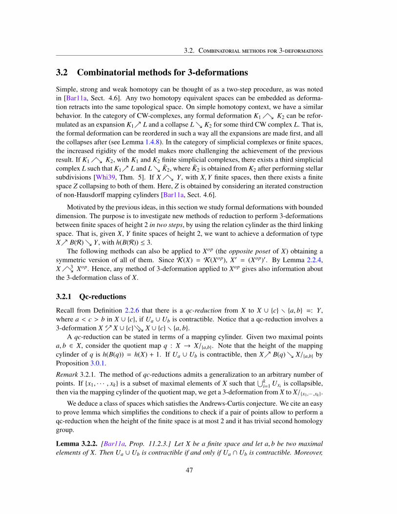
3.2. Combinatorial methods for 3-deformations

3.2 Combinatorial methods for 3-deformations

Simple, strong and weak homotopy can be thought of as a two-step procedure, as was notedin [Bar11a, Sect. 4.6]. Any two homotopy equivalent spaces can be embedded as deforma-tion retracts into the same topological space. On simple homotopy context, we have a similarbehavior. In the category of CW-complexes, any formal deformation K1 �↘ K2 can be refor-mulated as an expansion K1↗ L and a collapse L↘ K2 for some third CW complex L. That is,the formal deformation can be reordered in such a way all the expansions are made first, and allthe collapses after (see Lemma 1.4.8). In the category of simplicial complexes or finite spaces,the increased rigidity of the model makes more challenging the achievement of the previousresult. If K1 �↘ K2, with K1 and K2 finite simplicial complexes, there exists a third simplicialcomplex L such that K1↗ L and L↘ K2, where K2 is obtained from K2 after performing stellarsubdivisions [Whi39, Thm. 5]. If X �↘ Y , with X,Y finite spaces, then there exists a finitespace Z collapsing to both of them. Here, Z is obtained by considering an iterated constructionof non-Hausdorff mapping cylinders [Bar11a, Sect. 4.6].

Motivated by the previous ideas, in this section we study formal deformations with boundeddimension. The purpose is to investigate new methods of reduction to perform 3-deformationsbetween finite spaces of height 2 in two steps, by using the relation cylinder as the third linkingspace. That is, given X, Y finite spaces of height 2, we want to achieve a deformation of typeX↗ B(R)↘ Y , with h(B(R)) ≤ 3.

The following methods can also be applied to Xop (the opposite poset of X) obtaining asymmetric version of all of them. Since K(X) = K(Xop), X′ = (Xop)′. By Lemma 2.2.4,X �↘3 Xop. Hence, any method of 3-deformation applied to Xop gives also information aboutthe 3-deformation class of X.

3.2.1 Qc-reductions

Recall from Definition 2.2.6 that there is a qc-reduction from X to X ∪ {c} r {a, b} =: Y ,where a < c > b in X ∪ {c}, if Ua ∪ Ub is contractible. Notice that a qc-reduction involves a3-deformation X ↗e X ∪ {c}↘↘ X ∪ {c} r {a, b}.

A qc-reduction can be stated in terms of a mapping cylinder. Given two maximal pointsa, b ∈ X, consider the quotient map q : X → X/{a,b}. Note that the height of the mappingcylinder of q is h(B(q)) = h(X) + 1. If Ua ∪ Ub is contractible, then X↗ B(q)↘ X/{a,b} byProposition 3.0.1.

Remark 3.2.1. The method of qc-reductions admits a generalization to an arbitrary number ofpoints. If {x1, · · · , xk} is a subset of maximal elements of X such that

⋃ki=1 Uxi is collapsible,

then via the mapping cylinder of the quotient map, we get a 3-deformation from X to X/{x1,··· ,xk}.

We deduce a class of spaces which satisfies the Andrews-Curtis conjecture. We cite an easyto prove lemma which simplifies the conditions to check if a pair of points allow to perform aqc-reduction when the height of the finite space is at most 2 and it has trivial second homologygroup.

Lemma 3.2.2. [Bar11a, Prop. 11.2.3.] Let X be a finite space and let a, b be two maximalelements of X. Then Ua ∪ Ub is contractible if and only if Ua ∩ Ub is contractible. Moreover,

47

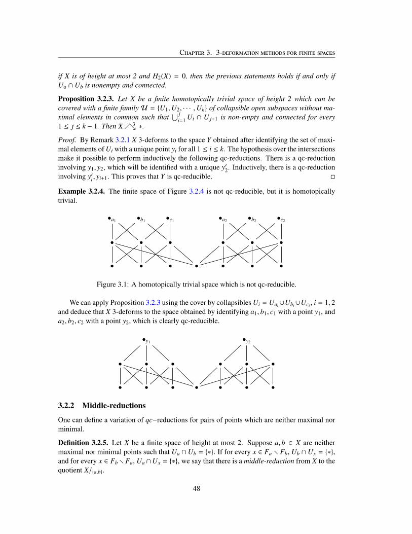
Chapter 3. 3-deformation methods for finite spaces

if X is of height at most 2 and H2(X) = 0, then the previous statements holds if and only ifUa ∩ Ub is nonempty and connected.

Proposition 3.2.3. Let X be a finite homotopically trivial space of height 2 which can becovered with a finite family U = {U1,U2, · · · ,Uk} of collapsible open subspaces without ma-ximal elements in common such that

⋃ ji=1 Ui ∩ U j+1 is non-empty and connected for every

1 ≤ j ≤ k − 1. Then X �↘3 ∗.

Proof. By Remark 3.2.1 X 3-deforms to the space Y obtained after identifying the set of maxi-mal elements of Ui with a unique point yi for all 1 ≤ i ≤ k. The hypothesis over the intersectionsmake it possible to perform inductively the following qc-reductions. There is a qc-reductioninvolving y1, y2, which will be identified with a unique y′2. Inductively, there is a qc-reductioninvolving y′i , yi+1. This proves that Y is qc-reducible. �

Example 3.2.4. The finite space of Figure 3.2.4 is not qc-reducible, but it is homotopicallytrivial.

•a1 •b1 •c1 •a2 •b2 •c2

• • • • • •

• • • • • • •

Figure 3.1: A homotopically trivial space which is not qc-reducible.

We can apply Proposition 3.2.3 using the cover by collapsibles Ui = Uai∪Ubi∪Uci , i = 1, 2and deduce that X 3-deforms to the space obtained by identifying a1, b1, c1 with a point y1, anda2, b2, c2 with a point y2, which is clearly qc-reducible.

•y1 •y2

• • • • • •

• • • • • • •

3.2.2 Middle-reductions

One can define a variation of qc−reductions for pairs of points which are neither maximal norminimal.

Definition 3.2.5. Let X be a finite space of height at most 2. Suppose a, b ∈ X are neithermaximal nor minimal points such that Ua ∩Ub = {∗}. If for every x ∈ Fa r Fb, Ub ∩Ux = {∗},and for every x ∈ Fb r Fa, Ua ∩Ux = {∗}, we say that there is a middle-reduction from X to thequotient X/{a,b}.

48

3.2. Combinatorial methods for 3-deformations

Example 3.2.6. Figure 3.2 illustrates a middle-reduction involving the points a, b.

• • • •

• •a •b •

• • •∗ • •

Figure 3.2: A space with a middle-reduction.

Proposition 3.2.7. Let X be a finite space of height at most 2. If there is a middle-reductionfrom X to X/{a,b}, then X �↘3 X/{a,b}.

Proof. Consider the mapping cylinder of the quotient map q : X → X/{a,b}. It is clear thath(B(q)) ≤ 3.We only need to show that q−1(Uq(x)) is contractible for every x ∈ X. Indeed,

q−1(Uq(x)) =

Ux ∪ Ub if x ≥ a, x � bUx ∪ Ua if x ≥ b, x � aUx in other case.

If x ≥ a, x ≥ b, then Ux ∪ Ub↘ Ux ∪ Ub r {z ∈ X : z ≤ x, z � b}. The latter is a finite space ofheight 1 with two maximal elements, x and b, and it is contractible if and only if Ux ∩ Ub is asingleton. A similar argument applies to x ≥ a, x � b. �

We say that a finite space X of height 2 is middle-reducible if it can be transformed into aconnected space with a unique middle point (i.e. a point of height one) by performing middle-reductions. I n particular, if X is middle-reducible, then X �↘3 ∗.

Example 3.2.8. The space of Figure 3.3 3-deforms to a point. Note that it does not haveneither weak points nor qc-reductions. However, the points a, b ∈ X allow to perform a middle-reduction from X to X/{a,b}, and the last space is collapsible.

• • •

•a • •b • • •

• • • •

Figure 3.3: A model of a 2-complex which 3-deforms to a point via a middle-reduction.

The previous ideas could be applied to the general case of a quotient q : X → X/{a,b} witha, b incomparable elements. But the main obstacle is that h(B(q)) could exceed 3 if h(a) , h(b).

49

Chapter 3. 3-deformation methods for finite spaces

Remark 3.2.9. Middle-reductions can also be generalized to an arbitrary number of points. If{x1, · · · , xk} is a subset of non-maximal and non-minimal elements of X such that

⋃ki=1 Uxi∪Ux

is contractible for every x ∈⋃k

i=1 Fxi , applying Corollary 3.1.4 we get a 3-deformation from Xto X/{x1,··· ,xk}.

3.2.3 Edge-reductions

We introduce now the method of edge reduction, which was motivated by the following exam-ple. Consider the contractible space P of Figure 3.4, which is obtained from a pentagon byidentifying the edges as indicated in the figure. This example appeared in Barmak’s book([Bar11a], Example 11.3.7).

Figure 3.4: Pentagon.

Barmak observed that this space is contractible (because it can be obtained by attaching a2-cell to the circle by means of a map which is homotopic to the identity) and that there wasno reduction method to prove that the finite space X(K) associated to the h-regular structure Kof Figure 3.5 is homotopically trivial.

Figure 3.5: h-regular structure of the Pentagon.

We will show that an edge reduction in a finite space of height 2 induces a 3-deformation,

50

3.2. Combinatorial methods for 3-deformations

and we will use edge reductions to prove that the finite space X(K) of Barmak’s example canbe 3-deformed to a point.

Definition 3.2.10. Let X be a finite space and let e = (a ≺ b) be an edge in the Hasse diagramH(X), with b a maximal element. If Ubre is contractible, we say that there is an edge-reductionfrom X to X r e.

Remark 3.2.11. To check if there is an edge-reduction involving e = (a ≺ b) in X, we have toverify the contractibility of Ub r e. Nevertheless, we can see that Ub r e↘↘ Ub/{x∈X:x≺b,x,a}, sothe contractibility of the first one is equivalent to the same property in the latter. The previousstrong collapse can be performed because the points covered by b in Ub r e are up beat points.

Proposition 3.2.12. Let X be a finite space of height less than or equal to 2. Let e = (a ≺ b)be an edge such that there is an edge-reduction from X to X r e. Then X �↘3 X r e.

Proof. Consider the mapping cylinder B(ι) of the inclusion ι : X r e → X. To check thatB(ι)↘ X, it suffices to verify that i−1(Ux) is contractible for every x ∈ X. Indeed,

i−1(Ux) =

Ux if x , bUb r e if x = b,

so the contractibility in both cases is evident. Finally, as h(B(ι)) = h(X) + 1, it holds thath(B(ι)) ≤ 3. �

Example 3.2.13 (Pentagon). Recall the pentagon P of Figure 3.4. Consider the h-regularstructure1 K of Figure 3.5. It easy to check that the edges e1 and e2 of the Hasse diagram ofX(K) satisfies the conditions of Definition 3.2.10 (see Figure 3.6).

•σ • • •τ • • • •

•a

e1e1e1e1e1e1e1e1

•b

e2e2e2e2e2e2e2e2

• • • • • • • •

• • •

Figure 3.6: Face poset associated to the h-regular structure K of the Pentagon.

1h-regular complexes were introduced in [BM08a] as an extension of the class of regular complexes. A cellularcomplex is said to be h-regular if the attaching map of each cell is a homotopy equivalence with its image and theclosed cells en are subcomplexes of K.

51

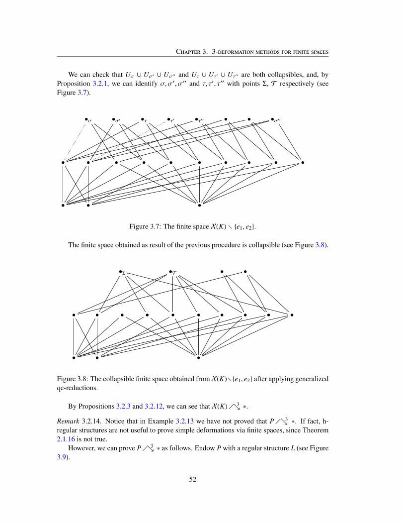
Chapter 3. 3-deformation methods for finite spaces

We can check that Uσ ∪ Uσ′ ∪ Uσ′′ and Uτ ∪ Uτ′ ∪ Uτ′′ are both collapsibles, and, byProposition 3.2.1, we can identify σ,σ′, σ′′ and τ, τ′, τ′′ with points Σ, T respectively (seeFigure 3.7).

•σ •σ′ •τ •τ′ •τ′′ • • •σ′′

• • • • • • • • • •

• • •

Figure 3.7: The finite space X(K) r {e1, e2}.

The finite space obtained as result of the previous procedure is collapsible (see Figure 3.8).

•Σ •T • •

• • • • • • • • • •

• • •

Figure 3.8: The collapsible finite space obtained fromX(K)r{e1, e2} after applying generalizedqc-reductions.

By Propositions 3.2.3 and 3.2.12, we can see that X(K)�↘3 ∗.

Remark 3.2.14. Notice that in Example 3.2.13 we have not proved that P�↘3 ∗. If fact, h-regular structures are not useful to prove simple deformations via finite spaces, since Theorem2.1.16 is not true.

However, we can prove P�↘3 ∗ as follows. Endow P with a regular structure L (see Figure3.9).

52

3.2. Combinatorial methods for 3-deformations

Figure 3.9: Regular cell structure of the Pentagon.

By Lemma 2.2.3, P�↘3 L. and we show that L�↘3 ∗. To begin with, we can performin X(L) two qc-reductions involving the pairs of 2-cells σ1, σ2 and τ1, τ2, and then performtwo point-reductions of the resultant up beat points s and t. As result, we obtain the face posetassociated to the h-regular K structure showed in Figure 3.5. Now, we can continue as weoutlined in Example 3.2.13.

3.2.4 Quotient reductions

In [Osa99], Osaki introduced two methods of reduction which allow one to find a quotient of agiven space with the same weak homotopy type. Namely, the quotient map q : X → X/Ux0 is aweak homotopy equivalence if Ux∩Ux0 is either empty or homotopically trivial for all x ∈ X. Inthis case, we say that there is a down O-reduction from X to X/Ux0 Similarly, q : X → X/Fx0 isa weak homotopy equivalence if Fx∩Fx0 is either empty or homotopically trivial. We say in thiscase that there is an up O-reduction. Barmak and Minian showed that, moreover, the quotientmaps are simple homotopy equivalences [BM07]. To prove this they used the mapping cylinderof the quotient map. That is, q : X → X/Ux0 (resp. q : X → X/Fx0) satisfies the hypothesis ofProposition 3.0.1, so X ↗γ B(q)↘↘ X/Ux0 (resp. X ↗γ B(q)↘↘ X/Fx0). In fact,

q−1(Uq(x)) =

Ux ∪ Ux0 if x ∈ Ux0

Ux if x < Ux0 .

It only remains to note that Ux ∩Ux0 is nonempty if and only if x ∈ Ux0 , and in that case, Ux ∪

Ux0↘↘ S(Ux ∩ Ux0), the non-Hausdorff suspension of Ux ∩ Ux0 . 2 The latter is homotopicallytrivial if and only if Ux ∩ Ux0 so is.

If the height of X is 2, the previous argument proves that X↗ B(q)↘↘ X/Ux0 (resp. thatX↗ B(q)↘↘ X/Fx0). In fact, as the homotopically trivial spaces of height at most one are

2Given X a finite topological space, the non-Hausdorff suspension of X is the finite space whose underlying setis X t S 0 in which we keep the given ordering in X and we set x ≤ y for every x ∈ X and y ∈ S 0. See [Bar11a, Def.2.7.1., Prop 2.7.3] for a more detailed exposition.

53

Chapter 3. 3-deformation methods for finite spaces

actually contractible, the γ-points are now weak points. However, it does not necessarily showthat there is a 3-deformation, because B(q) not always has height at most 3 (see Figure 3.10).

• •

• •x0

• •

X

•

• •

• • •

• •

• •

B(q)

•

• •

•

X/Ux0

Figure 3.10: A finite space X of height 2 with an Osaki’s reduction, where h(B(q)) = 4.

A proof using the relation cylinder will show that if h(X) = n and Ux0 satisfies Osaki’shypothesis, then X �↘

n+1X/Ux0 .

Theorem 3.2.15. Let X be a finite space of height n and let x0 ∈ X. If Ux ∩ Ux0 is empty orcontractible for every x ∈ X, then X �↘

n+1X/Ux0 .

Proof. Let R ⊆ X/Ux0 × X be the relation defined by q(x)Rx for every x ∈ X/Ux0 . If x ∈ X,then

R−1(UX

x

)= U

X/Ux0q(x) ,

which is contractible since it has maximum. Hence, by Proposition 3.1.2, K(B(R))↘ K(X).On the other hand, for every q(x) ∈ X/Ux0 ,

R

(F

X/Ux0q(x)

)=

FXx if x < Ux0 ,

UXx0 if x ∈ Ux0 .

In the first case, R(F

X/Ux0q(x)

)has minimum and then it is contractible. In the second case, we will

see that R(F

X/Ux0q(x)

)is collapsible by proving that UX

x0↘ UXx0

. Let {x1, x2, · · · , xk} be a linear

extension of UXx0 r UX

x0. For every 1 ≤ i ≤ k,

UUX

x0r{x1,x2,··· ,xi−1}

xi = Uxi ∩ UXx0.

54

3.2. Combinatorial methods for 3-deformations

Given that Uxi∩UXx0

is contractible, UXx0r{x1, x2, · · · , xi−1}↘ UX

x0r{x1, x2, · · · , xi−1, xi}. Thus,

we have proved that UXx0↘ UX

x0. Since UX

x0is collapsible, so is UX

x0 . By Proposition 3.1.3,K(B(R))↘ K(X).

It only remains to show that h(B(R)) ≤ n + 1 = h(X) + 1. Since h(X/Ux0) ≤ h(X), thisfollows from the fact that if q(x)Rx then hX/Ux0

(q(x)) ≤ hX(x). Thus, K(X)�↘n+1K(X/Ux0).

By Lemma 2.2.4, X �↘n+1

X/Ux0 . �

Corollary 3.2.16. If X is a finite space of height 2 and there is an up O-reduction from X toU/Ux0 , then X �↘3 X/Ux0 .

Proof. If there is an up O-reduction from X to U/Ux0 , then Ux ∩Ux0 is a homotopically trivialspace of height one, and then, contractible. Hence, Theorem 3.2.15 applies. �

In general a finite space X and its quotients do not have the same weak homotopy type. Wewill make a detailed study of the problem of determining whether a finite space X of height nsatisfies that it (n + 1)-deforms to a quotient X/A.

Recall that if X is a finite space and A ⊆ X is a subspace, then X/A is T0 if and only ifA ∩ A = A. That is, if for every a < b ∈ A, [a, b] ⊆ A (see [Bar11a, Prop. 2.7.8.]). Theorem3.2.15 can be generalized to arbitrary quotients X/A, with a similar proof, as follows.

Proposition 3.2.17. Let X be a finite space and A ⊆ X be a connected subspace space suchthat A ∩ A = A. If Fx ∪ A is homotopically trivial for every x ∈ A, then X �↘ X/A.

Remark 3.2.18. Suppose that we are in the hypothesis of Proposition 3.2.17, but we also knowthat FX

x ∪ A is collapsible for every x ∈ A. If q : X → X/A is the quotient map, define therelation R ⊆ X/A×X by q(x)Rx for all x ∈ X. From Propositions 3.1.2 and 3.1.3 we can deduceK(X)↗ K(B(R))↘ K(X/A).

Theorem 3.2.19. Let X be a finite space and A ⊆ X be a connected open subspace. If A ishomotopically trivial, then X �↘ X/A. Moreover, if A is collapsible, then X �↘

n+1X/A with

n = h(X).

Proof. If A is open, then it is clear that A ∩ A = A, so X/A is T0. Moreover, h(X/A) ≤ h(X).On the other hand, for every x ∈ A, Fx ⊆ A. Since A = A and A is homotopically

trivial, Fx ∪ A = A is homotopically trivial for every x ∈ A. Thus, by Proposition 3.2.17,X �↘ X/A. Moreover, if A is collapsible, by Remark 3.2.18, K(X)↗ K(B(R))↘ K(X/A),where R ⊆ (X/A) × X is the relation defined by q(x)Rx for every x ∈ X. It only remainsto see that h(B(R)) ≤ n + 1 = h(X) + 1. The length of a chain in B(R) involving x ∈ X ishX/A(q(x)) + hXop(x) + 1. But hX/A(q(x)) ≤ hX(x) and hX(x) + hXop(x) ≤ h(X). Thus, h(B(R)) ≤h(X) + 1. Finally, K(X)�↘

n+1K(X/A) and by Lemma 2.2.4, X �↘

n+1X/A. �

The following definitions are motivated by Proposition 3.2.19, being generalizations of theOsaki methods of reduction.

Definition 3.2.20. Let X be a finite space and A ⊆ X be a connected open subspace. If A ishomotopically trivial, we say that there is a generalized O-reduction from X to X/A.

55

Chapter 3. 3-deformation methods for finite spaces

Definition 3.2.21. Let X be a finite topological space of height at most 2 and A ⊆ X be aconnected open subspace. If A is collapsible, we say that there is a O-3-reduction from X toX/A.

Remark 3.2.22. If X is a finite space and A ⊆ X is an open subspace, then the fact that Ux∩A iseither homotopically trivial or empty for every x ∈ X implies that A↘γ A, with a similar proofof Theorem 3.2.15. Moreover, if Ux ∩ A is either contractible or empty for every x ∈ X, thenA↘ A. Therefore, if there is an (up) O-reduction from X to X/Ux0 then Ux0 is homotopicallytrivial and there is a generalized O-reduction from X to X/Ux0 .

Remark 3.2.23. If X has height at most 2, then A ∩ Ux is homotopically trivial for every x ∈ Aif and only if A↘ A by a sequence of down weak points.

In fact, suppose A↘e A r {x1} ↘e · · · ↘e A r {x1, x2 · · · , xn} = A where xi is a down weak

point of A r {x1, x2, · · · , xi−1}. Given x ∈ X, if x < A r A, it is clear that Ux ∩ A is eitherhomotopically trivial or empty. If x ∈ A r A, then x = xi is a down weak point of A r

{x1, x2, · · · , xi−1}. But

UAr{x1,x2,··· ,xi−1}xi =

(UX

xi∩ A

)⊔(UX

xi∩ (A r {x1, x2, · · · , xi−1}) ∩ Ac),

which is a contractible subspace of X of height at most 1. So, UXx ∩ A is contractible if and

only if it is connected. If UXxi∩ A was non-connected, as UA

y r {x1, x2, · · · , xi−1} is connected,there would exist a path connecting at least two components. So there exists x j ∈ Uxi ∩ A r

(A ∪ {x1, x2, · · · , xi−1}), with i < j ≤ n, an element in the path. But h(xk) = 1 and UAr{x1,··· ,xk−1}xk

has at least 2 elements. Therefore, xk cannot be a down weak point of A r {x1, x2, · · · , xk−1},which is a contradiction.

Remark 3.2.24. The O-3-reduction method provides a way to “simplify” regular CW-complexesunder 3-deformations. Let K be a regular CW-complex of dimension at most 2. Let e0 be a cellin K such that e0 ∩ e is either empty or contractible for every cell e ∈ K. By Theorem 3.2.19,X(K)�↘3 X(K)/Ue0 But the hypothesis also implies that K/e is again a regular CW-complex,and X(K)/Ue0 = X(K/e). By Lemma 2.2.3, it follows that K �↘3 K/e.

Hence, we get a method of reduction for regular CW-complexes of dimension at most 2that actually summarizes a 3-deformation.

Example 3.2.25. The finite space X of height 2 of Figure 3.11 is the wedge Y1 ∨y0 Y2 oftwo copies of a collapsible space Y whose unique weak point is exactly y0. Thus, X is ahomotopically trivial space without weak points, and even without any O-reduction. However,X can be 3-deformed into a single point. The closure of the open subset A = ∪5

i=1Uxi is triviallycollapsible. Thus, there is a generalized O-reduction from X to X/A, where the latter collapsesto Y2. Thus, X �↘3 ∗.

56

3.3. SAGE implementation.

•x1 •x2 •x3 •x4 •x5 •y0 • • • • •

• • • • • • • • • • • • • •

• • • • • •

Figure 3.11: A finite space without weak points with no O-reductions, but with generalizedO-reductions.

3.3 SAGE implementation.

We implemented each of the above described new methods of 3-deformation of finite spacesin the SAGE platform (see Appendix 3.A). The function random_core(X) makes use of allthese methods. It takes as input a finite space X of height less or equal than 2 and returns afinite space which 3-deforms to the original one. The output is a non-reducible finite spaceobtained after applying a sequence of reductions to X, whose order is chosen at random. Eachreduction corresponds to one of the methods previously developed (weak points, generalizedqc-reductions, middle-reductions, edge reductions, O-3-reductions). Of course, if the output isa single point, then X �↘3 ∗. However, the algorithm is not exhaustive.

In Figure 3.12 there is a sequence of random reductions allowing to 3-deform to a point thecontractible space of Example 2.2.7.

57

Chapter 3. 3-deformation methods for finite spaces

Figure 3.12: The program random_core applied to the Triangle.58

3.A. Appendix: 3-deformation SAGE module

3.A Appendix: 3-deformation SAGE module

Middle reduction

1 def is_middle_reduction(X, a, b):2 lower_intersection=Set(X.order_ideal([a])).intersection(Set(X.

order_ideal([b])))3 if len(lower_intersection) != 1:4 return False5 Fa_minus_Fb=Set(X.order_filter([a])).difference (Set(X.

order_filter([b])))6 for x in Fa_minus_Fb:7 if len(Set(X.order_ideal([b])).intersection(Set(X.

order_ideal([x])))) != 1:8 return False9 Fb_minus_Fa=Set(X.order_filter([b])).difference (Set(X.

order_filter([a])))10 for x in Fb_minus_Fa:11 if len(Set(X.order_ideal([a])).intersection(Set(X.

order_ideal([x])))) != 1:12 return False13 return True14

15 def is_middle_op_reduction(X, a, b):16 return is_middle_reduction(op(X),a, b)

Edge reduction

1 def is_down_edge(X, e): #e=[e[0], e[1]]2 if e[1] not in X.maximal_elements(): return False3 Y=remove_edge(U(X, e[1]), e)4 return is_contractible(Y)5

6 def is_up_edge(X,e):7 if e[0] not in X.minimal_elements(): return False8 Y=remove_edge(F(X, e[0]), e)9 return is_contractible(Y)

10

11 def is_reducible_edge(X, e):12 return is_up_edge(X, e) or is_down_edge(X, e)

Osaki reductions

1 def is_down_O_reduction(X, x):2 if len(X.order_ideal([x])) == 1: return False3 for y in X:4 intersection = Set(X.order_ideal([x])).intersection(Set(X.

order_ideal([y])))

59

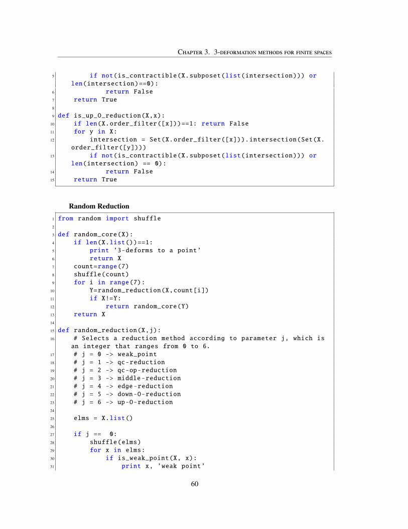
Chapter 3. 3-deformation methods for finite spaces

5 if not(is_contractible(X.subposet(list(intersection))) orlen(intersection)==0):

6 return False7 return True8

9 def is_up_O_reduction(X,x):10 if len(X.order_filter([x]))==1: return False11 for y in X:12 intersection = Set(X.order_filter([x])).intersection(Set(X.

order_filter([y])))13 if not(is_contractible(X.subposet(list(intersection))) or

len(intersection) == 0):14 return False15 return True

Random Reduction1 from random import shuffle2

3 def random_core(X):4 if len(X.list())==1:5 print ’3-deforms to a point’6 return X7 count=range(7)8 shuffle(count)9 for i in range(7):

10 Y=random_reduction(X,count[i])11 if X!=Y:12 return random_core(Y)13 return X14

15 def random_reduction(X,j):16 # Selects a reduction method according to parameter j, which is

an integer that ranges from 0 to 6.17 # j = 0 -> weak_point18 # j = 1 -> qc-reduction19 # j = 2 -> qc-op-reduction20 # j = 3 -> middle-reduction21 # j = 4 -> edge-reduction22 # j = 5 -> down-O-reduction23 # j = 6 -> up-O-reduction24

25 elms = X.list()26

27 if j == 0:28 shuffle(elms)29 for x in elms:30 if is_weak_point(X, x):31 print x, ’weak point’

60

3.A. Appendix: 3-deformation SAGE module

32 Y = remove_point(X, x)33 return Y34 return X35

36 if j == 1:37 M = X.maximal_elements()38 shuffle(M)39 for S in Set(M).subsets(2):40 l=list(S)41 if is_qc_reduction(X, l[0], l[1]):42 print l[0],l[1], ’qc-reduction’43 Y = quotient(X, [l[1], l[0]])44 return Y45 return X46

47 if j == 2:48 m = X.minimal_elements()49 shuffle(m)50 for S in Set(m).subsets(2):51 l = list(S)52 if is_qc_op_reduction(X, l[0], l[1]):53 print l[0], l[1], ’qc-op-reduction’54 Y = quotient_poset(X, [l[1], l[0]])55 return Y56 return X57

58 if j == 3:59 mid = [x for x in X.list() if not (x in X.maximal_elements()

or x in X.minimal_elements())]60 shuffle(mid)61 for S in Set(mid).subsets(2):62 l = list(S)63 if is_middle_reduction(X, l[0], l[1]):64 print l[0], l[1], ’middle-reduction’65 Y=quotient_poset(X, [l[1], l[0]])66 return Y67 return X68

69

70 if j == 4:71 E = X.cover_relations()72 shuffle(E)73 for e in E:74 if is_reducible_edge(X, e):75 print e, ’edge-reduction’76 Y = remove_edge(X, e)77 return Y78 return X79

61

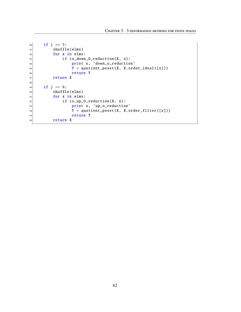
Chapter 3. 3-deformation methods for finite spaces

80 if j == 5:81 shuffle(elms)82 for x in elms:83 if is_down_O_reduction(X, x):84 print x, ’down_o_reduction’85 Y = quotient_poset(X, X.order_ideal([x]))86 return Y87 return X88

89 if j == 6:90 shuffle(elms)91 for x in elms:92 if is_up_O_reduction(X, x):93 print x, ’up_o_reduction’94 Y = quotient_poset(X, X.order_filter([x]))95 return Y96 return X

62

Resumen del capítulo 3: Métodos de 3-deformación de espacios fini-tos

En este capítulo estudiamos la formulación de la conjetura de Andrews-Curtis en el contexto deespacios finitos, es decir, el problema de decidir si un espacio finito homotópicamente trivialde altura 2 se 3-deforma a un punto. En general, no se conocen técnicas algorítmicas pararesolver este problema. Por nuestra parte, desarrollamos nuevos métodos de reducción deespacios finitos, que representan una 3-deformación de dos pasos, es decir, una deformaciónde tipo X↗ Y↘ ∗, donde la altura de Y es menor o igual que 3. Algunos ejemplos de losnuevos métodos desarrollados son: las reducciones de arista, las middle reducciones, y variosotros tipos de reducciones de tipo cociente, incluyendo las O-reducciones, una generalizacióny mejora de los métodos de reducción de Osaki [Osa99] para tipos homotópicos débiles deespacios finitos. Las reducciones disminuyen el número de puntos o aristas del diagrama deHasse asociado al poset, y se pueden describir en términos de la combinatoria este grafo. Alfinal del capítulo, se encuentra la implementación de nuestros métodos algorítmicos en SAGE.En particular, implementamos una función llamada random_core(X), que toma como input unespacio finito de dimensión 2 y devuelve como output el resultado de aplicarle al espacio unaserie de reducciones al azar de las antes mencionadas hasta llegar a un espacio irreducible.

Para lograr las 3-deformaciones de dos pasos, creamos un modelo finito llamado el cilindrono-Hausdorff de una relación R ⊆ X × Y entre espacios X e Y . Lo denotamos B(R). Si(x, y) ∈ R, lo denotamos por xRy.

Definición 3.1.1. Dada R ⊆ X × Y una relación, definimos el cilindro de una relación B(R)como el siguiente poset finito. El conjunto subyacente es la unión disjunta X tY . Preservamosel orden de X e Y y, para cada x ∈ X e y ∈ Y , decimos que x ≤ y en B(R) si existen puntosx′ ∈ X e y′ ∈ Y tales que x ≤ x′ en X, y′ ≤ y en Y y x′Ry′ (i.e. tomamos la relación generadapor x ≤ y si xRy).

Barmak y Minian prueban que se puede lograr una equivalencia simple entre dos espaciosfinitos X e Y mediante una función continua f : X → Y que cumpla ciertas características. Másaún, deformación se logra como X↗ B( f )↘ Y , donde B( f ) es el cilindro no-Hausdorff de lafunción f .

Proposición 3.0.1. (Barmak, Minian)[BM08b, 3.7] [Bar11a, 4.2.7, 6.2.10] Sea f : X → Y unafunción continua entre espacios finitos. Si f −1(Uy) (resp. f −1(Fy)) es contráctil para todo y inY , entonces B( f )↘ X.

Las siguientes proposiciones generalizan (y simetrizan) el resultado anterior para relacionesR entre dos espacios finitos X y Y . Nos sirvieron para formular 3-deformaciones del tipoX↗ B(R)→ Y .

Proposición 3.1.2. Sea R ⊆ X×Y una relación entre espacios finitos. Si R−1(Uy) es homotópi-

camente trivial para cada y ∈ Y , entonces B(R)�↘ X. Más aún, si para cada y ∈ Y , R−1(Uy)es colapsable, entonces K(B(R))↘ K(X).

63

Capitulo 3: Metodos de 3-deformacion de espacios finitos

Proposición 3.1.3. Sea R ⊆ X × Y una relación entre espacios finitos. Si R(Fx) es homotópi-camente trivial para cada x ∈ X, entonces B(R)�↘ Y . Más aún, si para cada x ∈ X, R(Fx) escolapsable, entonces K(B(R))↘ K(Y).

Los nuevos métodos de reducción que formulamos en esta tesis para estudiar la conjeturade Andrews-Curtis son descriptos a continuación.

Las middle-reducciones son una variación de las qc-reducciones para puntos no maximalesni minimales.

Definición 3.2.5. Sea X un espacio finito de dimensión a lo sumo 2. Supongamos que a, b ∈ Xson puntos no maximales ni minimales tales que Ua ∩ Ub = {∗}. Si para cada x ∈ Fa r Fb,Ub ∩Ux = {∗}, y para cada x ∈ Fb rFa, Ua ∩Ux = {∗}, decimos que hay una middle-reducciónde X al cociente X/{a,b}.

Proposición 3.2.7. Sea X un espacio finito de altura a lo sumo 2. Si hay una middle-reducciónde X a X/{a,b}, entonces X �↘3 X/{a,b}.

Las reducciones de arista permiten eliminar cierto tipo de arcos del diagrama de Hasse deun espacio finito.

Definición 3.2.10. Sea X un espacio finito y sea e = (a ≺ b) una arista del diagrama de HasseH(X), con b un elemento maximal. Si Ub r e es contrácl, decimos que hay una reducción dearista de X a X r e.

Proposición 3.2.12. Sea X un espacio finito de altura a lo sumo 2. Sea e = (a ≺ b) una aristatal que existe una reducción de X a X r e. Entonces X �↘3 X r e.

Como consecuencia de este nuevo método, pudimos hallar una 3-deformación explícitacon técnicas de espacios finitos del siguiente espacio que aparece al final del libro de Barmak[Bar11a], como un ejemplo de espacio homtópicamente trivial que no posee ninguna reducciónposible.

Figure 3.13: Estructura h-regular del Pentágono.

64

•σ • • •τ • • • •

•a

e1e1e1e1e1e1e1e1

•b

e2e2e2e2e2e2e2e2

• • • • • • • •

• • •

Figure 3.14: Face poset asociado a la estructura h-regular del Pentágono.

Un resultado relevante de este capítulo fue la prueba de que las reducciones de Osaki[Osa99] en espacios de dimensión son 3-deformaciones.

Teorema 3.2.15. Sea X un espacio finito de altura n y sea x0 ∈ X. Si Ux ∩ Ux0 es vacío ocontráctil para todo x ∈ X, entonces X �↘

n+1X/Ux0 .

Realizamos además un estudio general de reducciones dada por cociente. En general, unespacio finito X no tiene el mismo tipo homotópico débil que sus cocientes X/A, incluso si Aes contráctil. Hallamos una condición general sobre A que asegura que si X es de altura n,entonces X �↘

n+1X/A.

Teorema 3.2.19. Sean X un espacio finito de altura n, A ⊆ X un subespacio abierto conexo.Si A es homotópicamente trivial, entonces X �↘ X/A. Más aún, si A es colapsable, entoncesX �↘

n+1X/A.

65

Capitulo 3: Metodos de 3-deformacion de espacios finitos

66

Chapter 4

The Nerve Theorem

A very useful construction in algebraic topology and computational geometry is the notion ofnerve. For instance, it is the main tool to prove the Crosscut Theorem, the Dowker Theoremand Helly type theorems for intersection patterns of covers. Recently, there were found veryuseful applications in the area of topological data analysis, whose goal is to obtain informationabout the topology of a space from a discrete sample of the space.

The Nerve Theorem, due to Borsuk [Bor48] with alternative versions of Leray [Ler45],Weil (1952), Wu (1962), McCord (1967) and others, particularly guarantees that the nerve ofa family of geometric objects has the same homotopy type as the union of the objects, if theyform a good cover, that is, if the intersection of any subfamily is either empty or contractible.Nevertheless, this requirement is rather strong and not always adequate.

Many generalizations of the Nerve Theorem have been done since then (see [Bj"03, Bar11b]).We present a new result, obtained as a consequence of Propositions 3.1.2 and 3.1.3, which im-plies a new version of the Nerve Theorem.

4.1 A generalization of the classical Nerve Theorem

Recall that the nerve of a family U = {Ui}i∈I of subsets of a set X is the simplicial complexN(U) whose simplices are the finite subsets J ⊆ I such that

⋂i∈J

Ui , ∅.

Several versions of the Nerve Theorem can be found, involving convex sets in Rd or goodcovers of a topological space. We mention here a one version suitable for our purposes (see[Bar11b]).

Theorem 4.1.1 (Nerve Theorem). Let K be a finite simplicial complex (or a regular cell com-plex) and letU = {Li}i∈I be a finite family of subcomplexes of K such that

⋃i∈J Li = K. If every

intersection of elements ofU is empty or contractible, then K has the same (simple) homotopytype as N(U).

IfU is a cover of a simplicial complex K satisfying hypothesis of Theorem 4.1.1, thenUis said to be a good cover of K.

67

Chapter 4. The Nerve Theorem

Corollary 4.1.2. If X is a finite topological space andU = {Ui}i∈I is an open cover of X suchthat every intersection of elements ofU is empty or homotopically trivial, then X �↘ X(N(U)).

Proof. The family of simplicial complexes K(U) = {K(Ui)}i∈I is a cover by subcomplexesof K(X). The intersections are

⋂j∈J K(U j) = K(

⋂j∈J U j) for every J ⊆ I. Since

⋂j∈J U j is

either empty or homotopically trivial, then by Corollary 2.1.8 K(U) is a good cover of K(X).By Nerve Theorem 4.1.1, K(X)�↘ N(K(U)). Notice that N(K(U)) = N(U). By Theorem2.1.16, X′ �↘ X(N(U)). By Lemma 2.2.4, X �↘ X′. Thus, X �↘ X(N(U)). �

Remark 4.1.3. Corollary 4.1.2 is equivalent to the Nerve Theorem 4.1.1. In fact, ifU = {Li}i∈I

is a good cover of a simplicial complex K by a finite family of subcomplexes, then X(U) =

{X(Li)}i∈I is a good open cover of X(K).

Now we deduce from Propositions 3.1.2 and 3.1.3 a more general statement in which wedo not require the cover to be a good cover.

For simplicity, we will denote by N(U) the face poset of N(U), and we will call it thenon-Hausdorff nerve ofU.

Theorem 4.1.4. Let X be a finite topological space and letU = {Ui}i∈I be an open cover of X.Let N0(U) be the subspace of the non-Hausdorff nerve N(U) consisting of all homotopicallytrivial intersections. If for every x ∈ X, the subspace Ix of N0(U) of the intersections whichcontain x, is homotopically trivial, then X has the same simple homotopy type as N0(U).

Proof. For every J ⊆ I, denote IJ =⋂

i∈J Ui. So the elements of N0(U) are the subsets J ⊆ Isuch that IJ is homotopically trivial.

Define the relation R ⊆ X × N0(U)op as follows: for every x ∈ X and J ⊆ I such that IJ ishomotopically trivial, set

x R IJ if x ∈ IJ .

On the one hand,R−1

(UIJ

)= IJ = IJ ,

which is homotopically trivial by construction of N0(U).On the other hand,

R(Fx) = {IJ : IJ 3 y for some y ≥ x} = {IJ : IJ 3 x} = {IJ : x ∈ IJ} = Ix,

which is homotopically trivial by hypothesis.Thus, by Propositions 3.1.2 and 3.1.3, X �↘ N0(U)op. Since N0(U)op �↘ N0(U), we

deduce that X �↘ N0(U). �

Remark 4.1.5. If U = {Ui}i∈I is a good cover of a finite space X then N(U) = N0(U). More-over, for every x ∈ X, the subspace of N(U) of the intersections containing x has a maximumelement, the intersection

⋂Ui∈UUi3x

Ui and, namely then it is homotopically trivial. Thus, the Nerve

Theorem for posets 4.1.2 can be deduced from Theorem 4.1.4.

68

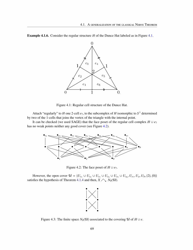
4.1. A generalization of the classical Nerve Theorem

Example 4.1.6. Consider the regular structure H of the Dunce Hat labeled as in Figure 4.1.

Figure 4.1: Regular cell structure of the Dunce Hat.

Attach “regularly” to H one 2-cell e7, to the subcomplex of H isomorphic to S 1 determinedby two of the 1-cells that joins the vertex of the triangle with the internal point.

It can be checked (we used SAGE) that the face poset of the regular cell complex H ∪ e7has no weak points neither any good cover (see Figure 4.2).

•e1 •e2 •e3 •e4 •e5 •e6 •e7

• • • • • • •a •b

•1 •2 •0

Figure 4.2: The face poset of H ∪ e7.

However, the open cover U = {Ue1 ∪ Ue2 ∪ Ue3 ∪ Ue4 ∪ Ue5 ∪ Ue6 ,Ue7 ,Ua,Ub, {2}, {0}}satisfies the hypothesis of Theorem 4.1.4 and then, X �↘ N0(U).

• •

• •

• •

Figure 4.3: The finite space N0(U) associated to the coveringU of H ∪ e.

69

Chapter 4. The Nerve Theorem

We investigate now some conditions on covers, which are easy to check, that imply thehypotheses of Theorem 4.1.4.

Definition 4.1.7. A family U of open subspaces of a finite space X is called a quasi-goodcover if every nonempty intersection of a subfamily ofU has homotopically trivial connectedcomponents.

Definition 4.1.8. Given a finite space X and a cover U = {Ui}i∈I of X, define M(U) the finitespace whose elements are the connected components C of

⋂i∈J Ui for every J ⊆ I, with the

order given by C ⊆⋂

i∈J Ui < C′ ⊆⋂

i∈J′ Ui if J ⊆ J′ and C ⊇ C′.

Corollary 4.1.9. Let X be a finite space and letU be a quasi-good cover of X. Then, X �↘M(U).

Proof. Define U′ = U⋃{C : C , ∅ connected component of

⋂i∈J Ui}J⊆I a new cover of X.

Notice that M(U) = N0(U′). For every x ∈ X, the subspace Ix of N0(U′) of the intersectionscontaining x has a minimum: the connected component containing x of the maximal subset J ⊆I such that x ∈

⋂i∈J Ui, Thus, Ix is homotopically trivial. By Theorem 4.1.4, X �↘ N0(U′)

and the result follows. �

To get an intuition, if U is a quasi-good cover, N(U) not necessarily encodes the simplehomotopy type of X, but it is enough to replace every element

⋂i∈J Ui of N(U) by its connected

components, preserving the order given by the reversed inclusion of the subsets, and get a newfinite space M(U) satisfying X �↘ M(U).

Example 4.1.10. Let X be the finite model of S 1 with 6 points of Figure 4.4. Although X isnot a minimal finite model of S 1, it has not beat point nor weak points. Even more, there doesnot exists any cover of X with open subspaces satisfying the Nerve Theorem 4.1.2 hypothesis.

•3 •4 •5

•0 •1 •2

Figure 4.4: A finite model of S 1.

However,U = {U3 ∪U4,U5} is a quasi-good cover of X, since (U3 ∪U4) ∩U5 = {1} ∪ {2}has two contractible connected components. Despite the fact that N(U) does not encodes thesimple homotopy type of X, by of Corollary 4.1.9, we can deduce that X is simply equivalentto M(U), which is actually the minimal model of S 1.

70

4.2. Applications to (n + 1)-deformations

• •

•

N(U)

• •

• •

M(U)

Figure 4.5: The finite spaces N(U) and M(U) associated to a quasi-good coverU of X.

Theorem 4.1.4 and Corollary 4.1.9 have their counterparts in the context of complexes.

Theorem 4.1.11. Let K be a finite simplicial complex (or a regular cell complex) and letU = {Li}i∈I be a finite family of subcomplexes of K such that

⋃i∈J Li = K. Denote by N0(U)

to the subcomplex of N(U)′ whose simplices are the chains of contractible intersections. Iffor every σ ∈ K, the subcomplex S σ of N0(U) of chains with elements all containing σ iscontractible, then K has the same simple homotopy type as N0(U).

Notice that ifU is a covering of a simplicial complex K whose all nonempty intersectionsare contractible, then N0(U) = N(U)′ �↘ N(U), and the contractibility of the complexesS σ is trivially satisfied since they are cones with apex

⋂Li∈ULi3σ

Li. Thus, Nerve Theorem 4.1.1 is a

particular case of Theorem 4.1.11.

Corollary 4.1.12. Let K be a finite simplicial complex (or a regular cell complex) and letU = {Li}i∈I be a finite family of contractible subcomplexes of K such that

⋃i∈J Li = K and

every nonempty intersection of a subfamily has contractible connected components. Then,K �↘ M(U), whereM(U) = K(M(U)).

4.2 Applications to (n + 1)-deformations

The goal of this section is to find deformations with an upper bound on the dimensions of theinvolved spaces, by means of the Nerve Theorem.

A first preliminary remark is that is we replace the condition of “homotopically trivial” by“collapsible” in the statement of Theorem 4.1.4, we get that X↗ B(R)↘ N0(U), with R is therelation defined in the proof of the theorem. However, the construction of N0(U) is not suitableto preserve low dimension.

We define the reduced version of the non-Hausdorff nerve, which fixes the redundancy ofintersections IJ = IJ′ with J , J′.

Definition 4.2.1. Let X be a finite topological space and let U = {Ui}i∈I be a finite coverof X by open subspaces. Define the reduced non-Hausdorff nerve N(U) by the poset of allthe non-empty finite spaces obtained as intersections of elements of the cover U, ordered byinclusion.

71

Chapter 4. The Nerve Theorem

Remark 4.2.2. Note that N(U)↘↘ N(U). In fact, we can define an equivalence relation in theset of subsets J of I such that IJ , ∅. We say that J ∼ J′ if IJ = IJ′ . For every J, let J0 bethe union of all the elements in the equivalence class of J. In particular, J0 ∼ J. Thus, we canstrong collapse

N(U)↘↘ N(U) r {IJ : J ∼ J0, J , J0}

by removing successively the maximal elements of {IJ : J ∼ J0, J , J0} since they are up beatpoints. The previous strong collapses can be done simultaneously for all the representatives J0of the equivalence classes.

Theorem 4.2.3. Let X be a finite poset of height less or equal to n and let U = {Ui}i∈I be anopen cover of X such that N0(U), the subspace of N(U) of collapsible intersections, is again ofheight less or equal to n. If for every x ∈ X, the subspace Ix of N0(U) of the intersections whichcontain x is collapsible and its height is less or equal than n − hX(x), then X �↘

n+1N0(U).

Proof. We follow the main idea of the proof of Theorem 4.1.4. Define the relation R ⊆ X ×N0(U)op as follows: for every x ∈ X and I ∈ N0(U), set

x R I if x ∈ I.

R satisfies hypothesis of Propositions 3.1.2 and 3.1.3. Thus, X↗ B(R)↘ N0(U)op. Notethat m = h(N0(U)) ≤ h(X) = n and N0(U)op �↘

m+1N0(U). So we only have to see that

h(B(R)) ≤ n + 1. A maximal chain in B(R) is c = x1 < x2 < · · · < xr < I1 < I2 < · · · < Is

with x1 < x2 < · · · < xr a maximal chain in Uxr ⊆ X, I1 a minimal element in the subspace ofN0(U)op of the intersections which contain xr and I1 < I2 < · · · < Is a maximal chain in thatsubspace. Since, by hypothesis s ≤ n−r, the length of c is less or equal than r+1+n−r = n+1.Therefore, h(B(R)) ≤ n + 1 and X �↘

n+1N0(U). This completes the proof. �

Definition 4.2.4. A familyU of open subsets of a finite space X is said a collapsible quasi-goodcover if every nonempty intersection of a subfamily has collapsible connected components.

Given a finite space X and a quasi-good cover U = {Ui}i∈I of X, denote by M(U) thefinite space whose elements are the topological spaces obtained as the connected componentsof

⋂i∈J Ui for some J ⊆ I, ordered by inclusion.

Corollary 4.2.5. Let X be a finite space of height n and letU = {Ui}i∈I be a collapsible quasi-good cover of X. If h(M(U)) ≤ n and the minimal connected component of the intersectionsof elements of U which contains an element x ∈ X is of height less or equal than h(x), thenX �↘

n+1M(U).

Example 4.2.6 (Dunce Hat). Consider the regular structure H of the Dunce Hat described inFigure 4.1. Take the following cover U = {Ue1 ∪ Ue2 ,Ue3 ∪ Ue4 ,Ue5 ,Ue6} of X(H) by fourcollapsible open subspaces. Since U a collapsible quasi-good cover of X(H), by Corollary4.1.9, X(H)�↘ M(U) (see Figure 4.6).

72

4.2. Applications to (n + 1)-deformations

• • • •

• • • • • • • • • • • •

• • • • • • • • • • • •

• • •

Figure 4.6: The finite space M(U) associated to a quasi-good cover of the Dunce Hat.

Moreover, the cover U also satisfies the hypothesis of height imposed in Corollary 4.2.5.Thus,X(H)�↘3 M(U), and the latter again collapsible. Finally, H �↘3 H′ �↘3 K(M(U))↘ ∗.This shows that H 3-deforms to a single point.

•U1 •U2 •U3 •U4

•a •b •c •d •>> •>

•3 •2 •1

Figure 4.7: The finite space M(U) associated to a collapsible quasi-good coverU of the DunceHat.

73

Chapter 4. The Nerve Theorem

74

Resumen del capítulo 4: El Teorema del Nervio

SeaU = {Ui}i∈I una familia de subconjuntos de un conjunto X. El nervio deU es el complejosimplicial N(U) cuyos símplices son los subconjuntos finitos J ⊆ I tales que

⋂i∈J

Ui , ∅.

El Teorema del Nervio, probado por Borsuk [Bor48], garantiza que el nervio de una familiade espacios tiene el mismo tipo homotópico que la unión de los espacios si éstos forman uncubrimiento bueno, es decir, si la intersección de toda subfamilia es vacía o contráctil.

Teorema 4.1.1 (Teorema del Nervio). Sea K un complejo simplicial finito, (o complejo celularregular) y sea U = {Li}i∈I una familia finita de subcomplejos de K tales que

⋃i∈J Li = K.

Si toda intersección de elementos de U es vacía o contráctil, entonces K tiene el mismo tipohomotópico (simple) que N(U).

El Teorema del Nervio es equivalente a la siguiente formulación para espacios finitos. DadoU un cubrimiento finito por abiertos X, el nervio no-Hausdorff deU es el face poset del nervioclásico N(U). Lo denotamos por N(U).

Corolario 4.1.2. Si X es un espacio topológico finito yU = {Ui}i∈I es un cubrimiento abiertode X tal que toda intersección de elementos deU es vacía u homotópicamente trivial, entoncesX �↘ X(N(U)).

El siguiente resultado es una generalización del teorema anterior, en el cual permitimos alcubrimiento tener intersecciones no vacías no contráctiles.

Teorema 4.1.4. Sea X un espacio topológico finito y sea U = {Ui}i∈I un cubrimiento abiertode X. Sea N0(U) el subespacio del nervio no-Hausdorff N(U) de todas las interseccioneshomotópicamente triviales. Si para todo x ∈ X, el subespacio Ix ⊆ N0(U) de las interseccionesque contienen a x es homotópicamente trivial, entonces X �↘ N0(U).

Decimos que una familiaU de subespacios de un espacio finito X es un cubrimiento cuasi-bueno si toda intersección no vacía de una subfamilia de U tiene sus componentes conexashomotópicamente triviales. El siguiente resultado que a partir de cubrimientos quasi-buenostambién se pueden extraer modelos finitos de un espacio.

Denotamos por M(U) al espacio finito cuyos elementos son las componentes conexas decada intersección de elementos deU, con el orden dado por la inclusión.

Corolario 4.1.9. Sea X un espacio finito y seaU un cubrimiento cuasi-bueno de X. Entonces,X �↘ M(U).

Por otra parte, realizamos aplicaciones de los resultados anteriores al estudio de (n + 1)-deformaciones. Para optimizar la altura del modelo finito que se puede obtener a partir deun cubrimiento U, definimos N(U), el nervio no-Hausdorff reducido. Se puede ver queN(U)↘↘ N(U).

Definición 4.2.1. Sea X un espacio topológico finito y seaU = {Ui}i∈I un cubrimiento finito deX por subespacios finitos. Definimos el nervio no-Hausdorff reducido N(U) como el poset detodos los espacios finitos no vacíos obtenidos como intersección de elementos del cubrimientoU, ordenados por inclusión.

75

Capitulo 4: El Teorema del Nervio

Probamos los siguientes resultados.

Teorema 4.2.3. Sea X un espacio finito de altura menor o igual que n, y sea U = {Ui}i∈I uncubrimiento abierto de X tal que N0(U), el subespacio de N(U) de intersecciones colapsables,es también de altura menor o igual que n. Si para cada x ∈ X, el subespacio Ix de N0(U) de lasintersecciones que contienen a x es colapsable y de altura menor o igual que n−hX(x), entoncesX �↘

n+1N0(U).

Dados X un espacio finito y U = {Ui}i∈I un cubrimiento cuasi-bueno de X, denotamospor M(U) al espacio finito cuyos elementos son los espacios topológicos obtenidos como lascomponentes conexas de

⋂i∈J Ui para algún J ⊆ I, ordenadas por inclusión.

Corolario 4.2.5. Sean X un espacio finito de altura n yU = {Ui}i∈I un cubrimiento cuasi-buenode X cuyas intersecciones no vacías son colapsables. Si h(M(U)) ≤ n y las componentesconexas minimales de intersecciones de elementos deU que contienen un elemento x ∈ Xtienen altura menor o igual que h(x), entonces X �↘

n+1M(U).

Ejemplo 4.2.6 (Dunce Hat). Considerar la estructura regular H para el Dunce Hat descripta enla Figura 4.8.

Figure 4.8: Estructura celular regular para el Dunce Hat.

Tomar el siguiente cubrimiento U = {Ue1 ∪ Ue2 ,Ue3 ∪ Ue4 ,Ue5 ,Ue6} de X(H) por cuatrosubespacios abiertos colapsables. Dado queU es un cubrimiento cuasi-bueno colapsable, porCorolario 4.1.9, X(H)�↘ M(U) (ver Figure 4.9).

76

• • • •

• • • • • • • • • • • •

• • • • • • • • • • • •

• • •

Figure 4.9: El espacio finito M(U) asociado a un cubrimiento cuasi-bueno del Dunce Hat.

Más aún, el cubrimientoU también satisface las hipótesis de altura de del Corolario 4.2.5.Luego, X(H)�↘3 M(U). El último espacio es también colapsable. Finalmente, H �↘3 H′ �↘3 K(M(U))↘ ∗. Esto prueba que H se 3-deforma a un punto.

•U1 •U2 •U3 •U4

•a •b •c •d •>> •>

•3 •2 •1

Figure 4.10: El espacio finito M(U) asociado a un cubrimiento cuasi-buenoU del Dunce Hat.

77

Capitulo 4: El Teorema del Nervio

78

Chapter 5

Homotopy colimits and deformations

5.1 Homotopy colimits

Limits and colimits are fundamental constructions in mathematics. They naturally arise as ageneralization of well known concepts as cartesian products, disjoint unions and direct sums.However, when the category in question has a “homotopy theory” limits and colimits are gen-erally not homotopically well-behaved. For example, in general they are not invariant underhomotopy equivalences. Thus, it is convenient to obtain a replacement with better properties,usually called a “homotopy limit” and “homotopy colimit”.

We are interested in studying the homotopy type of the colimit of diagrams of topologicalspaces.

Let I be a small category and C any category. Recall that a I-diagram in a category C isjust a functor X : I → C. The category I is called the indexing category and gives the shapeto the diagram. The actual objects and morphisms of I are irrelevant, but only the way theyare interrelated is meaningful. Thus, a diagram X can be thought of as a collection {X(i)}i∈I ofobjects and morphisms {X(α) : X(i) → X( j)}α:i→ j in C patterned on I. For simplicity, denoteXi := X(i).

The colimit of a diagram X : I → C (if it exists) is an object colim X in C equipped withmorphisms φi : Xi → colim X for every i ∈ I such that φ jX(α) = φi for each α : i → jmorphism in I,

Xi

φi &&

X(α) //

�

X j

φ jxxcolim(X)

and satisfies the following universal property: for every Z ∈ C together with morphisms ψi :Xi → Z for every i ∈ I such that ψ jX(α) = ψi for each α : i → j morphism in I, there exists a

79

Chapter 5. Homotopy colimits and deformations

unique morphism F : colim(X)→ Z such that Fφi = ψi for every i ∈ I.

Xi

�

φi &&

ψi

$$

X(α) //

�

X j

�

φ jxx

ψ j

zz

colim(X)

∃!F

��Z

If C is the category of topological spaces, then colim X always exists and it is homeomorphicto ⊔

j∈J

X j/ ∼

where ∼ is the equivalence relation generated by x ∈ Xi ∼ X(α)(x) ∈ X j for every α : i → jmorphism in I. For instance, if the indexing category is depicted by 0→ 1, then colim(X) of the

diagram X0f // X1 is isomorphic to X1. If, instead, we index on the “push out category”,

with three objects and two non-identity maps: 1 ← 0 → 2, then colim(X) is precisely the

push out of the diagram X1 X0foo g // X2 , which is homeomorphic to X1 t X2/ ∼, where

f (x) ∼ g(x) for every x ∈ X0. In particular, if X2 = {∗}, then colim X is homeomorphic toX1/ f (X0).

Given X,Y : I → C two I-diagrams in C, a morphism of diagrams ϕ : X → Y is just anatural transformation from X to Y . That is, for every i ∈ I, there is a map φ j : X j → Y j suchthat if α : i→ j is a morphism in I, then the following diagram commutes.

X j

�

ϕ j // Y j

Xi

X(α)

OO

ϕ j// Yi

Y(α)

OO

Notice that if X and Y are diagrams of topological spaces, a morphism ϕ : X → Y induces acontinuous map ϕ : colim X → colim Y . But if ϕi : Xi → Yi is a homotopy equivalence forevery i ∈ I, unfortunately it does not follow in general that ϕ is a homotopy equivalence. Hereis an example, let X,Y be the diagrams Dn ← S n−1 → Dn, ∗ ← S n−1 → ∗ respectively, indexedon 1 ← 0 → 2, with n ≤ 2. Let ϕ : X → Y be the natural transformation which is the identityon S n−1 and collapses Dn to a point. Then colim X � S n, but colim Y � ∗.

In conclusion, there are natural transformations which are objectwise homotopy equiva-lences, but the homotopy inverses of its components may not fit together into a natural trans-formation. So the colimit functor does not necessarily preserves homotopy equivalences, thatis, it is not a homotopy invariant.

80

5.1. Homotopy colimits

The homotopy colimits arise because of the previous basic difficulty, as a “correction” ofthe colimit to be homotopy invariant. There are simple examples of homotopy colimit construc-tions, which had been widely used, even before of the development of the theory. For instance,

the homotopy colimit of a diagram of topological spaces X0f // X1 with indexing category

0 → 1 is precisely (homeomorphic to) the mapping cylinder of f , which deformation retractsto X1. On the other hand, the homotopy colimit of a diagram indexed on the pushout category1← 0→ 2 is the so called homotopy pushout, which is constructed by gluing together X1 andX2 “up to homotopy”. Specifically, hocolim X � X1 t (X0 × I) t X2/ ∼, where (x, 0) ∼ f (x)and (x, 1) ∼ g(x) for every x ∈ X0. In particular, if f : A → X is a map and the diagram is∗ ← A→ X, then the homotopy pushout is homeomorphic to the mapping cone of f .

In the example of the diagrams X,Y described by Dn ← S n−1 → Dn and ∗ ← S n−1 → ∗

indexed both on 1← 0→ 2, is easy to check that hocolim X ' hocolim Y ' S n.

There are two things to point out from the previous examples, which have been mimicked inthe general theory. On the one hand, whereas the colimit of a diagram of spaces is constructedby merely gluing them, the homotopy colimit is obtained by gluing them up to homotopy,being a “fattened up” version of the classic colimit. On the other hand, note that there is a maphocolim X → colim X obtained by collapsing the homotopies. Under some conditions, thismap is a homotopy equivalence.

The construction is due to Bousfield & Kan [BK72] and, independently, to Vogt [Vog73].We will only work with homotopy colimit indexed by (finite) posets. In this case, the homotopycolimits are easier to define.

Let P be a finite a poset, viewed as a small category with a unique arrow p → q for eachp, q ∈ P such that p ≤ q, and let X : P → Top be a P-diagram of topological spaces. Recallthat if p ∈ P, Fp = {q ∈ P : q ≥ p}. The homotopy colimit of X, hocolim X, is defined by⊔

p∈P

|K(Fp)| × Xp/ ∼

where ∼ is the following equivalence relation. For every p ≤ q ∈ P, we have a continuousmap fpq : Xp → Xq and an inclusion i : |K(Fq)| → |K(Fp)|. The relation ∼ is generated by(α, fp,q(x)) ∈ |K(Fq)| × Xq ∼ (i(α), x) ∈ |K(Fp)| × Xp, for every x ∈ Xp, α ∈ |K(Fq)|.

Let I be a small category and let X : I → CAT be a functor to the category CAT of smallcategories. Recall that the Grothendieck construction on X, which is usually denoted by I

∫X,

is the following category. The objects are the pairs (i, x), where i is an object of I and x is aobject of X(i), and the morphisms (α, β) : (i, x)→ (i′, x′) are given by morphisms α : i→ i′ inI and β : X(α)(x)→ x′ in X(i′).

Now, given any small category I, its nerve N(I) is a simplicial set whose n-simplices arethe sequences of n composable morphisms in I. The geometric realization of this simplicial setis a topological space, called the classifying space of the category I.

Thomason’s theorem [Tho79] establishes the existence of a natural homotopy equivalencebetween the nerve of the Grothendieck construction and the homotopy colimit of N(X) (here

N(X) is the diagram of simplicial sets given by the composition I X // CAT N // SS of Xwith the nerve functor).

81

Chapter 5. Homotopy colimits and deformations

Theorem 5.1.1 (Thomason). Let I be a small category and CAT the category of small cate-gories. If X : I → CAT is an I-diagram of small categories, then there is a natural homotopyequivalence

hocolimN(X)→ N(I∫

X).

In particular, the previous result says that the homotopy colimit of a diagram of topologicalspaces combinatorially described as the nerve of certain small categories has itself a combina-torial description as the nerve of a single category (namely, the Grothendieck construction ofthe diagram).

5.2 The Grothendieck construction on posets and non-Hausdorffhomotopy colimits

Working with diagrams over finite posets will allow us to apply combinatorial methods to studytheir homotopy colimits. We also refer the reader to [Zv93] and [WZv99] for applications ofhomotopy colimits to combinatorial problems.

Let P be a finite poset and let X be a P-diagram of finite posets, i.e. a functor from P to thecategory P<∞ of finite posets. In this case the Grothendieck construction on X can be describedas a poset as follows.

Definition 5.2.1 (The non-Hausdorff homotopy colimit of finite posets). Let X : P → P<∞ bea functor. The non-Hausdorff homotopy colimit of X, denoted by hocolim X, is the followingposet. The underlying set is the disjoint union

∐p∈P Xp. We keep the given ordering within Xp

for all p ∈ P, and for every x ∈ Xp and y ∈ Xq such that p ≤ q, we set x ≤ y in hocolim X iffpq(x) ≤ y in Xq. Here Xp = X(p) for each p ∈ P and fpq = X(p→ q) for each p ≤ q in P.

By Thomason’s theorem we have a homotopy equivalence

K(hocolim X) ' hocolim KX,

since the nerve of a poset viewed as a small category is in fact its order complex.In the context of finite posets, Thomason’s theorem can be deduced from a more general

result. This will be proved in Theorem 5.4.3.

Remark 5.2.2. The homotopy colimit of diagrams of finite posets can be thought as an iteratedconstruction of the cylinder of a relation in the following way.

Let p1, p2, · · · , pn be a linear extension of P (i.e., an ordering of the elements of P suchthat if pi ≤ p j, then i ≤ j). Denote Xi = Xpi for all 1 ≤ i ≤ n. Define B0 = X0 and, inductively,Bi = B(Ri) for all 1 ≤ i ≤ n, where Ri ⊆ Bi−1 × Xi is the relation defined by xRi fppi(x) for allp < pi ∈ P, for each x ∈ Xp. Then, hocolim X = Bn.

Remark 5.2.3. At this point it is worth noting the difference between hocolim X and hocolim Xfor a given diagram X : P → P<∞. The first one is the Grothendieck construction on X andit is a finite poset (which can be viewed as a finite topological space). The second one is theclassical construction of homotopy colimit of a diagram of topological spaces (applied, in this

82

5.2. The Grothendieck construction on posets and non-Hausdorff homotopy colimits

case, to a diagram of finite topological spaces) and it is not a finite space. However, as animmediate consequence of Theorem 5.4.3, we will see that they are weak equivalent spaces(when we view hocolim X as a finite topological space).

A very first and important example of non-Hausdorff homotopy colimit is the non-Hausdorffmapping cylinder.

Example 5.2.4. Any map f : X0 → X1 between finite posets can be viewed as a diagramX : 1 → P<∞ where 1 is the poset of two elements 0 < 1. Similarly as in the topologicalcontext, we have hocolim X = B f , the non-Hausdorff mapping cylinder of f .

Now we will reinterpret some well-known results about homotopy colimits reinterpreted inthe non-Hausdorff setting (see [BK72, Seg68, tD71, Vog73]). We give direct and elementaryproofs of their statements in this context.

Recall that given X a P-diagram, colim X =⋃

p∈P Xp/ ∼, where x ∼ fpp′(x) for all x ∈ Xp

and p ≤ p′ in P. Note that colim X is not always a poset. A necessary and sufficient conditionis that if x, y ∈ Xp are non-comparable and fpp′(x) < fpp′(y) for some p′ > p, then for allp′′ > p, either fpp′′(x) < fpp′′(y) or they are non-comparable.

The following lemma is a version of the Projection Lemma for diagrams over posets.

Lemma 5.2.5 (Projection Lemma). Let P be a finite poset and A a finite collection of opensubposets of P, ordered by inclusion. Let X : (A,⊆)→ P<∞ be the associated diagram, definedby X(A) = A for all A ∈ A, and X(A ≤ A′) the inclusion map ıAA′ . If for every A, A′ ∈ A,either A ∩ A′ = ∅ or A ∩ A′ is union of elements ofA, then hocolim X =

⋃A∈A A (viewed as a

subposet of P) and hocolim X↘↘ colim X.

Proof. Let A1, A2, · · · , An be a linear extension of (A,⊆). For simplicity, if A j ⊆ Ai, denote byı ji the inclusion map.

Define inductively Y0 = hocolim X, Yi = Yi−1 r(⋃

A j⊆Ai ı ji(A j))

for all 1 ≤ i ≤ n. Notethat colim X (which is homeomorphic to Yn) is a subposet of hocolim X (= Y0). We will showinductively that Yi↘↘ Yi+1 for all 0 ≤ i ≤ n − 1.

Suppose {A j : j < i} are disjoints, and iterate the following reasoning. Take x ∈ Ai aminimal element of

⋃A j⊆Ai ı ji(A j) ⊆ Ai. Then, there exists a unique j < i such that x ∈ A j, and

UYi−1x = UYi−1

ı−1ji (x)

has maximum element. Hence Yi−1↘↘e Yi−1 r {x}. �

The Homotopy Lemma is actually the statement that guarantees that homotopic colimitsare invariant under homotopies.

Lemma 5.2.6 (Homotopy Lemma). Let P be a finite poset and let X,Y : P → P<∞ be twoP-diagrams of finite posets. If α : X → Y is a morphism of diagrams such that αp : Xp → Yp

is a weak equivalence for all p ∈ P, then α induces a weak equivalence

hocolim X 'we

hocolim Y.

The proof of the Homotopy Lemma can be deduced from the original Homotopy Lemmafor diagrams of spaces and Thomason’s theorem. However, we will show a direct proof inRemark 5.3.3 using combinatorial methods.

The following result is a reformulation of the Wedge Lemma [Zv93].

83

Chapter 5. Homotopy colimits and deformations

Lemma 5.2.7 (Wedge Lemma). Let X : P → P<∞ be P-diagram of finite posets. If for eachp ∈ P, there exists cp ∈ Xp such that fqp(x) = cp for all x ∈ Xp′ and p′ ≤ p in P, then

hocolim X 'we

P ∨∨p∈P

Xp ∗ Fp,

where the wedge is formed by identifying cp ∈ Xp ∗ Fp with p ∈ P.

Björner, Wachs and Welker [BWW05] deduced a generalization of Quillen’s Fiber Lemma2.1.10 for maps not satisfying that the preimage of the minimal open sets is always homotopi-cally trivial. We translate this result into the poset setting. The idea of the proof is the same asthe original.

Theorem 5.2.8 (Björner, Wachs, Welker). Let f : P→ Q be an order preserving map betweenfinite posets such that for all q ∈ Q, the fiber f −1(Uq) is non-empty, and for all non-minimalq ∈ Q the inclusion map f −1(Uq) ↪→ f −1(Uq) is weak homotopic to a constant map whichsends f −1(Uq) to cq for some cq ∈ f −1(Uq). Then

P 'we

Q ∨∨q∈Q

f −1(Uq) ∗ Fq,

where the wedge is formed by identifying each q ∈ Q with cq.

Proof. LetA be the collection of subposets of P given by { f −1(Uq) : q ∈ Q}, and let X : Q →P<∞ be the associated diagram. By the Projection Lemma 5.2.5, hocolim X↘↘ colim X ≡ P.On the other hand, define Y : Q → P<∞ by Y(q) = f −1(Uq) with Y(q′ ≤ q) the constant mapcq. By the Homotopy Lemma 5.2.6 for the diagrams K(X) and K(Y), K(X) ' K(Y), and thenhocolim X '

wehocolim Y . Finally, by the Wedge Lemma 5.2.7,

hocolim Y 'we

Q ∨∨q∈Q

f −1(Uq) ∗ Fq.

We will show now that P � colim X↗↗ hocolim X. The idea is similar to the proof of theProjection Lemma 5.2.5. Let q1, q2, · · · , qn be a linear extension of Q. Define Y0 = hocolim X,and inductively Yi+1 = Yi r f −1(Uqi), where f −1(Uqi) is thought as a subspace of f −1(Uqi).Note that P � Yn =

⋃q∈Q f −1({q}) ⊆ Y0.

To see that Yi↘↘ Yi+1, take x a minimal element of f −1(Uqi) ⊆ f −1(Uqi), and supposeXq j = f −1(q j) for all j ≤ i. Since f −1(Uqi) =

⊔q j≤qi f −1(q j), UYi

x has maximal element. �

5.3 Methods of reduction for non-Hausdorff homotopy colimits

We will use reduction methods to derive old and new results on homotopy colimits, whichwill allow us to compute in a direct and easy way the homotopy type of homotopy colimits ofdiagrams over posets.

As we note in Chapter 3, if f : X → Y is a map of posets, the non-Hausdorff mappingcylinder B f strong collapses to Y . This result will be viewed as a particular case of Corollary

84

5.3. Methods of reduction for non-Hausdorff homotopy colimits

5.3.2 below: if the indexing poset P has maximum p, the homotopy colimit of any P-diagramcollapses to Xp.

On the other hand, we also note in Proposition 3.0.1 that if f : X → Y is a poset mapsuch that f −1(Uy) is weakly contractible for every y ∈ Y , then f is a weak equivalence (i.e. itinduces a homotopy equivalence between the classifying spaces). This is Quillen’s Theorem Afor posets [Qui72] and McCord’s theorem [McC66] for finite topological spaces. In Proposition5.3.5 we will generalize this result for homotopy colimits of P-diagrams. Moreover, Quillen’sTheorem A for posets will follow immediately from Propositions 5.3.5 and 5.3.1 by applyingthe results to the poset 1.

Let X : P → P<∞ be a P-diagram of finite posets. The following statement relates thehomotopy type of P with the homotopy type of hocolim X. Notice that P↘↘ {p} does notimplies that hocolim X↘↘ Xp. For example, the homotopy pushout is indexed on the pushoutcategory P defined by 1 ← 0 → 2, which collapses to 1 for example. Nevertheless, hocolim Xnot necessarily is homotopic to X1. See the example of the diagram Dn ← S n−1 → Dn, whosehomotopy colimit is homotopic to S n. Now, if make a distinction between up and down beatpoints during the collapses, we can deduce collapses on the homotopy colimit.

Proposition 5.3.1. Let X : P → P<∞ be a P-diagram of finite posets. If p ∈ P is an up beatpoint, then hocolim X↘↘ hocolim X|Pr{p}. In particular, they are weak equivalent.

Proof. Let x0, x1, · · · , xn be a linear extension of Xopp , the opposite poset of Xp. Let Y0 =

hocolim X and for each 0 ≤ i ≤ n define inductively Yi+1 = Yi r {xi}. Let q be the minimumelement of FP

p . Note that FYixi = FYi

fpq(xi). This implies that xi is an up beat point of Yi for all

1 ≤ i ≤ n and therefore

hocolim X = Y0↘↘ Y1↘↘ · · ·↘↘ Yn+1 = (hocolim X) r Xp = hocolim X|Pr{p}.

�

Corollary 5.3.2. Let X : P→ P<∞ be P- diagram of finite posets. If P has a maximum elementp, then hocolim(X)↘↘ Xp. In particular, they are weak equivalent.

Proof. Let p = p0, p1, · · · , pn be a linear extension of Pop. Since P has a maximum element,there is a sequence of collapses

P↘↘ P r {p1}↘↘ P r {p1, p2} · · ·↘↘ P r {p1, p2, · · · , pn} = {p},

where pi is an up beat point of P r {p1, p2, · · · , pi−1}. By applying recursively Proposition5.3.1, we have

hocolim X↘↘ (hocolim X) r Xp1↘↘ · · ·↘↘ (hocolim X) rn⋃

i=1

Xpi = Xp.

�

85

Chapter 5. Homotopy colimits and deformations

Remark 5.3.3. From the previous result and McCord’s Theorem 2.1.9 we deduce an alternativeproof of the Homotopy Lemma 5.2.6. For any p ∈ P consider hocolim X|Up the homotopycolimit of the diagram restricted to Up. Since p is the maximum of Up, by Proposition 5.3.2hocolim X|Up↘ Xp and therefore α induces a weak equivalence hocolim X|Up 'we

hocolim Y |Up .Now the result follows from McCord’s Theorem 2.1.9 applied to the basis-like open cover{hocolim Y |Up}p∈P of hocolim Y .

Remark 5.3.4. Note that all the collapses in Proposition 5.3.1 and Corollary 5.3.2 are strongcollapses, in the sense that all the points removed are beat points (not just weak points). Thisimplies that if the finite space Xp in Corollary 5.3.2 is contractible then so is hocolim X.

Proposition 5.3.5. Let X : P → P<∞ be a P- diagram of finite posets. If p is a down beatpoint of P dominated by an element q and f −1

qp (Ux) is contractible for every x ∈ Xp, thenhocolim(X)↘ hocolim(X|Pr{p}). In particular they are weak equivalent.

Proof. Let x0, x1, · · · , xn a linear extension of Xp. Define Y0 = hocolim X, and inductivelyYi+1 = Yir {xi} for every 0 ≤ i ≤ n. We will show that Y0↘ Y1↘ · · · ↘ Yn+1 = (hocolim X)rXp.

Note that UYixi = hocolim Xi, where Xi : UP

p → P<∞ is the functor defined by Xi(p′) =

f −1p′p(Uxi), for all p′ < p in P (where the transition maps are induced by the original transition

maps).Since UP

p has a maximum element q and f −1qp (Uxi) is contractible, by Corollary 5.3.2 and

Remark 5.3.4, UYixi is a contractible finite space. This proves that xi is a weak point of Yi. �

Given a poset map φ : P → Q and a Q-diagram X, we denote by φ∗X the P-diagramobtained by pulling back X along φ. Concretely, φ∗X = Xφ. There is a canonical maphocolim φ∗X → hocolim X induced by the identities (φ∗X)p = Xφ(p). If i : Q′ → Q is asubposet and X is a Q-diagram, the restriction i∗X is what we have denoted by X|Q′ . Note thatin this case hocolim X|Q′ is a subposet of hocolim X.

Proposition 5.3.6. Let X : P→ P<∞ be a P- diagram of finite posets. If p is a down beat pointof P dominated by q and fqp is a weak equivalence, then

hocolim X 'we

hocolim X|Pr{p}.

Proof. Since p is dominated by q, there is a well defined strong homotopy retraction r : P →P r {p} which is the identity for any p′ , p and r(p) = q. Denote by i : P r {p} → Pthe inclusion. There is a morphism of P-diagrams γ : (ir)∗X → X such that γp′ is the iden-tity for every p′ , p and γp = fqp : ((ir)∗X)p = Xq → Xp. By hypothesis and Corollary5.2.6, γ induces a weak equivalence hocolim(ir)∗X '

wehocolim X, and by Proposition 5.3.5,

hocolim(ir)∗X 'we

hocolim X|Pr{p}. �

Example 5.3.7. By the previous proposition one can immediately deduce that the non-Hausdorff

86

5.3. Methods of reduction for non-Hausdorff homotopy colimits

homotopy pushout of the poset diagram

X0f1 //

f2��

X1

X2

is weak equivalent to X0 provided the maps f1 and f2 are weak equivalences.

We prove now an analogue, in the context of posets, of a cofinality theorem of Bousfieldand Kan. We need first a generalization of Proposition 5.3.1.

Proposition 5.3.8. Let X : P → P<∞ be a P-diagram of finite posets. If p is a point of P suchthat Fp is homotopically trivial, then hocolim X '

wehocolim X|Pr{p}.

Proof. Let x1, x2, · · · , xn be a linear extension of Xopp . For each 1 ≤ i ≤ n, we define the Fp-

diagram Xi : Fp → P<∞ as follows. Set Xi(p′) = F fpp′ (xi) and Xi(p′ → p′′) = fp′p′′ |F fpp′ (xi):

F fpp′ (xi) → F fpp′′ (xi).Given that Xi(p′) is contractible for all p′ ∈ Fp, by Corollary 5.2.6 one can see that

hocolim Xi 'we

Fp, and by hypothesis, the last one is homotopically trivial. Therefore, since

F(hocolim X)r{x1,x2,··· ,xi−1}xi = hocolim Xi,

which is homotopically trivial, we can remove the points x1, . . . , xn of Xp one by one, similarlyas in the proof of Proposition 5.3.1, and the result follows. �

We give now a direct and simple proof of a cofinality theorem for posets. This is a particu-lar case of a known result for functors between small categories which satisfy the hypotheses ofQuillens’s Theorem A and it is an analogue of Bousfield-Kan’s cofinality theorem in the com-binatorial setting. The key tool of the proof is the construction of the cylinder of an appropriaterelation.

Theorem 5.3.9 (Cofinality Theorem). Let ϕ : P → Q be an order preserving map betweenfinite posets. Let X : Q → P<∞ be a Q-diagram. If ϕ−1(Fq) is homotopically trivial for allq ∈ Q, then the canonical map hocolimϕ∗X → hocolim X is a weak equivalence.

Proof. LetR ⊆ Q×P the relation defined by φ(p)R p for every p ∈ P and construct the relationcylinder B(R) (see Definition 3.1.1). Consider the following B(R)-diagram X : B(R) → P<∞.For each q ∈ Q take X(q) = Xq, set X(p) = Xϕ(p) for p ∈ P, X(p → p′) = X(ϕ(p) → ϕ(p′)),X(q → q′) = X(q → q′), and X(ϕ(p) → p) = idXϕ(p) . Note that the restriction of X to Q is theoriginal diagram X and the restriction of X to P is ϕ∗X.

Take a linear extension q1, q2, · · · , qm of Qop. For each 1 ≤ j ≤ m we have

FB(R)r{q1,q2,··· ,q j−1}q j = ϕ−1(Fq j)

which is homotopically trivial by hypothesis. By applying recursively Proposition 5.3.8, weget hocolim X '

wehocolimϕ∗X.

87

Chapter 5. Homotopy colimits and deformations

Similarly, take a linear extension p1, p2, · · · , pn of P. For each 1 ≤ i ≤ n we have

UB(R)r{p1,p2,··· ,pi−1}pi = ϕ(Upi) = Uϕ(pi).

Therefore, pi is a down beat point of Rr {p1, p2, · · · , pi−1} dominated by ϕ(pi), and X(ϕ(pi)→pi) is the identity. By Proposition 5.3.5 we have hocolim X '

wehocolim X. �

If X : P→ P<∞ is a P-diagram of finite posets, in some cases we can recover the homotopytype of P from the homotopy type of hocolim X.

Proposition 5.3.10. Let X : P→ P<∞ be a P-diagram of finite posets. If hocolim X↘↘ ∗, thenP↘↘ ∗.

Proof. Let x1, x2, x3, · · · , xm be a sequence of points of hocolim X such that hocolim X↘↘hocolim X r {x1}↘↘ hocolim X r {x1, x2}↘↘ · · ·↘↘ hocolim X r {x1, x2 · · · , xm} = {∗}. Let{xi j} be the subsequence of {xi} of the last beat point removed of Xp for every p ∈ P. Forevery xi j , let Xp j the poset of the diagram X such that xi j ∈ Xp j . Finally, is easy to check thatP↘↘ P r {p1}↘↘ P r {p1, p2}↘↘ · · ·↘↘ P r {p1, p2, · · · , pn−1} = {pn}, with n = |P|. �

5.4 Variations on Thomason’s theorem and applications

We prove a result that relates the homotopy colimit of a diagram of spaces with the non-Hausdorff homotopy colimit of the diagram of their models. As a consequence we obtainan alternative and simple proof of Thomason’s theorem in the context of posets. As anotherimmediate consequence of the main result we deduce that the homotopy colimit of a diagramof finite simplicial complexes is weak equivalent to the non-Hausdorff homotopy colimit ofthe diagram of their face posets. This implies that all the techniques developed in the previoussection for non-Hausdorff homotopy colimits can be used for diagrams of polyhedra (indexedby finite posets) by means of the face poset functor.

We denote by Top the category of topological spaces and continuous maps. Sometimes werequire a diagram of spaces D : P→ Top to satisfy extra conditions (for instance D could be adiagram of simplicial complexes, finite topological spaces, etc), however in all these cases thehomotopy colimit D is taken in the category Top.

Theorem 5.4.1. Let P be a finite poset. Let K : P → Top be a diagram of spaces andX : P → P<∞ be a diagram of finite posets. Let φ : K → X be a diagram morphism (whereX is viewed as a diagram of finite topological spaces) such that φp : Kp → Xp is a weakequivalence for every p ∈ P. Then there exists a weak equivalence

φ : hocolim K → hocolim X.

Proof. We define first the map φ : hocolim K → hocolim X. For every p ≤ p′ denote byfpp′ = K(p → p′) and gpp′ = X(p → p′) the transition maps. Recall that hocolim K canbe constructed from the disjoint union

∐p∈P Kp × K(Fp) by identifying the pairs (α, β) ∈

Kp ×K(Fp) with (α′, β′) ∈ Kp′ ×K(Fp′) if fpp′(α) = α′ and β = β′ ∈ K(Fp′). We denote by ∼the equivalence relation generated by this identification.

88

5.4. Variations on Thomason’s theorem and applications

For each p ∈ P, let µp : K(Fp) → Fp ⊆ Xp be the McCord map (see Definition 2.1.5).Given (α, β) ∈ Kp × K(Fp) we define

φ(α, β) = φµp(β)( fpµp(β)(α)) ∈ Xµp(β) ⊆ hocolim X.

It is easy to verify that φ is well defined. In order to see that it is a continuous map, it sufficesto prove that for each y ∈ hocolim X, φ−1

(Uhocolim X

y

)∩

(Kq × K(Fq)

)is open in Kq × K(Fq)

for every q ∈ P. Fix y ∈ hocolim X and let p ∈ P such that y ∈ Xp. Note that φ−1(Uhocolim X

y

)∩(

Kq × K(Fq))

is empty if q � p and it is equal to (gqpφq)−1(UXp

y

)× µ−1

q

(UFq

p

)if q ≤ p. This

proves that φ is continuous.In order to prove that φ is a weak homotopy equivalence, we use McCord’s theorem 2.1.9

for the basis-like open cover{hocolim X|Up

}p∈P

of hocolim X. We have to see that

φ : φ−1(hocolim X|Up

)→ hocolim X|Up

is a weak equivalence for each p. Note that φ−1(hocolim X|Up) =∐

q≤p Kq × µ−1q (UFq

p )/ ∼ andthat there is a commutative diagram

Kp × {p}φp //

i��

Xp

j

��(∐q≤p Kq × µ

−1q

(UFq

p

)/ ∼

) φ // hocolim X|Up

.

The inclusion j is a weak equivalence by Corollary 5.3.2 and φp is a weak equivalence byhypothesis, thus we only need to check that the inclusion i is a homotopy equivalence.

Consider the retraction r :(∐

q≤p Kq × µ−1q

(UFq

p

)/ ∼

)→ Kp × {p} defined by r(α, β) =

( fqp(α), p) for (α, β) ∈ Kq×µ−1q

(UFq

p

). It is clear that ri = 1. We define a homotopy H : ir ' 1 as

a composition of two linear homotopies. Any β ∈ µ−1q

(UFq

p

)can be written as β = tβ1 +(1− t)β2

with 0 < t ≤ 1, β1 ∈ K(Up) and β2 ∈ K(Xp r Up). Take H1((α, β), s) = (α, (1 − s)β + sβ1).Since β1 ∈ K(Up) which is a cone with apex p, we can define then H2((α, β), s) = (α, (1 −s)β1 + sp). �

Remark 5.4.2. Under the hypotheses of Theorem 5.4.1, there is an alternative way to prove thathocolim K and hocolim X are weakly equivalent by means of a zigzag of weak equivalences.First one can see that it is enough to reduce to the case K = X and φ = 1X . Then, in order toprove that hocolim X and hocolim X are weakly equivalent one can use Thomason’s theorem(to obtain a weak equivalence at the level of simplicial sets) and McCord’s theorem (to comeback to the context of topological spaces). Theorem 5.4.1 exhibits an explicit and direct weakequivalence hocolim K → hocolim X.

As a first immediate corollary we obtain the following particular case of Thomason’s theo-rem for posets.

89

Chapter 5. Homotopy colimits and deformations

Corollary 5.4.3. Given a diagram of finite posets X : P → P<∞, there is a homotopy equiva-lence

hocolimKX → K(hocolim X).

Proof. Apply Theorem 5.4.1 to the diagram morphism µ : KX → X, where µp : K(Xp)→ Xp

is the McCord map. �

Remark 5.4.4. From Theorem 5.4.1 one can easily deduce that if X : P→ Top is a diagram offinite topological spaces, although hocolim X and hocolim X are very different, there is a weakhomotopy equivalence hocolim X → hocolim X induced by the identity map.

Now we prove a kind of converse of Thomason’s result, which relates the homotopy colimitof a diagram of simplicial complexes with the non-Hausdorff homotopy colimit of their faceposets.

Corollary 5.4.5. Let K : P→ Top be a diagram of finite simplicial complexes. Then there is aweak equivalence

ν : hocolim K → hocolim(XK)op

from the homotopy colimit of K to the non-Hausdorff homotopy colimit of the diagram of theopposite of their face posets.

Proof. Apply Theorem 5.4.1 to the diagram morphism induced by the natural weak equiva-lences νp : Kp → X(Kp)op defined in Remark 2.1.7. �

Since for every simplicial complex L, K(X(L)op) = K(X(L)) = L′ (the barycentric subdi-vision of L), from Corollary 5.4.3 and Corollary 5.4.5 we prove invariance of homotopy typeunder barycentric subdivision for homotopy colimits in the (general) unordered setting.

Corollary 5.4.6. Let K : P → Top be a diagram of (unordered) finite simplicial complexes(and simplicial maps). Then hocolim K and hocolim K′ are homotopy equivalent, where K′ :P→ Top is the diagram of the barycentric subdivisions (of spaces and maps).

Remark 5.4.7. It is well known that for any simplicial set T , there is a natural homotopy equi-valence sd T → T from the (geometric realization of the) barycentric subdivision of T to T(see for example [May12, Thm 12.2.5]). By Bousfield-Kan’s homotopy lemma [BK72], thisimplies that the homotopy colimit of a diagram of simplicial sets is homotopy equivalent tothe homotopy colimit of the diagram of their barycentric subdivisions. On the other hand, anyordered simplicial complex K (i.e. a simplicial complex together with a partial ordering of itsvertices that restricts to a total ordering on the vertices of each simplex) can be seen as a sim-plicial set Ks. Moreover, the simplicial set associated to its (geometric) barycentric subdivision(K′)s is naturally isomorphic to sd Ks, the subdivision of the simplicial set Ks (see [May12,Thm 12.2.2]). This proves that the homotopy colimit of a diagram of ordered simplicial com-plexes (and ordered simplicial maps) is homotopy equivalent to the homotopy colimit of thediagram of their barycentric subdivisions. However, in a general geometric situation, one hasto deal with diagrams of unordered simplicial complexes, and in the unordered context thereis no natural homotopy equivalence between K and its barycentric subdivision K′. Concretely,the homotopy equivalence of the last corollary cannot be deduced directly from a diagram map

90

5.4. Variations on Thomason’s theorem and applications

between K and K′ since, although the underlying topological spaces of Kp and K′p are equaland the transition maps fqp and f ′qp are (linearly) homotopic, in the context of unordered sim-plicial complexes there is no natural homotopy equivalence from the barycentric subdivisionfunctor to the identity functor. Moreover, in general the homotopies fqp ' f ′qp cannot be takencoherently.

Corollary 5.4.5 allows one to apply the results of the previous section to homotopy col-imits of diagrams of polyhedra, by means of the weak equivalence with the non-Hausdorffhomotopy colimits of the opposite of the face posets. In particular, the following analogues ofPropositions 5.3.8 and 5.3.6 are valid for diagrams of simplicial complexes.

Proposition 5.4.8. Let K : P→ Top be a diagram of finite simplicial complexes (and simplicialmaps). If p is a point of P such that Fp is homotopically trivial (in particular if p is an up beatpoint or an up weak point), then hocolim K ' hocolim K|Pr{p}.

Proof. Consider the diagram (XK)op : P→ P<∞, (XK)op(p) = (X(Kp))op, and apply Proposi-tion 5.3.8 and Corollary 5.4.5. �

Proposition 5.4.9. Let K : P→ Top be a diagram of finite simplicial complexes (and simplicialmaps). If p is a down beat point of P dominated by q and fqp is a homotopy equivalence, then

hocolim K ' hocolim K|Pr{p}.

Proof. Consider the diagram (XK)op : P → P<∞ and apply Proposition 5.3.6 and Corollary5.4.5. �

Suppose that K : P → Top is a diagram of finite simplicial complexes such that all thetransition maps fqp : Kq → Kp are homotopy equivalences (in particular, if P is connected, allKp have the same homotopy type). In general, although the simplicial maps fqp : Kq → Kp arehomotopy equivalences, the homotopy type of Kp and the topology of K(P) do not determinethe homotopy type of hocolim K. We will show that if the indexing poset P and the maps fqp

satisfy nice conditions, then hocolim K ' Kp (for any p ∈ P).

Corollary 5.4.10. Let K : P → Top be a diagram of finite simplicial complexes (and sim-plicial maps). If P is a contractible finite space and the transition maps fqp are homotopyequivalences, then hocolim K ' Kp (for any p ∈ P).

Proof. Since P is a contractible finite space, there is a sequence p1, · · · , pn such that pi is abeat point (up or down) of P r {p1, p2, · · · , pi−1} and P r {p1, p2, · · · , pn} = {p}. Now applyrecursively Propositions 5.4.8 and 5.4.9. �

As we remarked in the second chapter, if P is contractible (as a finite space) then its cla-ssifying space K(P) is contractible but the converse does not hold. Suppose that the indexingposet P can be reduced to a single point by removing γ-points (recall that p is a γ-point if Fp orUp is homotopically trivial). In that case the previous corollary is not longer valid since Propo-sition 5.4.9 works only for down beat points (i.e. when Up has maximum, not just homotopi-cally trivial). However, one can impose extra conditions on the maps fqp : Kq → Kp in order to

91

Chapter 5. Homotopy colimits and deformations

extend Proposition 5.4.9 to γ-points, and Corollary 5.4.10 to a more general class of homotopi-cally trivial posets. To this end we replace homotopy equivalences by contractible mappings.This class of maps was introduced by Cohen in [Coh67]. A simplicial map f : K → L is calleda contractible mapping if the preimage f −1(z) is contractible for every point z in the underlyingspace of L. In [Coh67, Thm 11.1] Cohen proved that any contractible mapping f : K → Lis a simple homotopy equivalence. In [Bar11b, Thm 5.1] Barmak exhibited an alternative andsimple proof of Cohen’s result. From the proof of [Bar11b, Thm 5.1] one can deduce thefollowing.

Proposition 5.4.11 (Barmak). Let f : K → L be a contractible mapping and letX( f )op : X(K)op → X(L)op be the map induced in the opposite of their face posets. Then(X( f )op)−1(Uσ) is homotopically trivial for every σ ∈ X(L)op.

Corollary 5.4.12. Let K : P → Top be a P-diagram of finite simplicial complexes (and sim-plicial maps). If p is a point of P such that Up is homotopically trivial and the transition mapsfqp are contractible mappings for every q ≤ p, then hocolim K ' hocolim K|Pr{p}.

Proof. Consider the diagram (XK)op : P → P<∞ and follow the proof of Proposition 5.3.5,using that (X( fqp)op)−1(Uσ) are homotopically trivial by Proposition 5.4.11. �

Corollary 5.4.12 in combination with Proposition 5.4.8 allows us to extend Corollary 5.4.10to a more general class of (homotopically trivial) indexing posets, under the stronger assump-tion that the transition maps are contractible mappings.

Corollary 5.4.13. Let K : P→ Top be a P-diagram of finite simplicial complexes. If the index-ing poset P can be reduced to a point by removing γ-points (in particular, if P is collapsible),and the transition maps fqp are contractible mappings, then hocolim K ' Kp (for any p ∈ P).

Example 5.4.14. If the transition maps of the following diagram of simplicial complexes arecontractible mappings, its homotopy colimit is homotopy equivalent to any of the Kp. This isbecause the indexing poset is a collapsible (but non-contractible) finite space.

K1

�� $$

K2

zz %%

K3

yy %%

K4

yy ��K5

�� ((

K6

�� ��

K7

�� ��

K8

vv ��K9 K10 K11

92

Resumen del capítulo 5: Colímites homotópicos y deformaciones

La teoría de colímites homotópicos fue intrducida independientemente por Bousfield y Kan[BK72] y Vogt [Vog73] como una “corrección” de la noción usual de colímite, para que, porun lado, cumpla la propiedad de ser invariante por homotopía, y por el otro, tenga el mismotipo homotópico que el colímite usual bajo buenas propiedades en el diagrama.

En este capítulo, usamos un teorema clásico de McCord y métodos de reducción de espa-cios finitos para probar una generalización del teorema de Thomason [Tho79] sobre colímiteshomotópicos de diagramas sobre posets. En particular, esto permite caracterizar los colímiteshomotópicos de diagramas de complejos simpliciales en términos de la construcción de Gro-thendieck de los diagramas de sus face posets. También deducimos análogos de resultadosconocidos sobre colímites homotópicos en el contexto combinatorio, incluyendo el teoremacofinal y una generalización del Teorema A de Quillen para posets.

Sea I una categoría pequeña, y sea X : I → CAT un funtor a la categoría de categoríaspequeñas. La construcción de Grothendieck en X, denotada por I

∫X, es la categoría cuyos

objetos son los pares (i, x), con i un objeto de I y x un objeto de X(i), y cuyos morfismos sonde la forma (α, β) : (i, x) → (i′, x′) con α : i → i′ un morfismo en I y β : X(α)(x) → x′ unmorfismo en X(i′). El teorema de Thomason [] afirma que existe una equivalencia homotópicanatural

hocolimN(X)→ N(I∫

X)

entre el colímite homotópico del nervio de X y el nervio de la construcción de Grothendiecken X.

En este capítulo, nos enfocamos en colímites homotópicos de diagramas de espacios in-dexados en posets. La idea es usar la interacción entre combinatoria y topología que lograla teoría de espacios topológicos finitos para estudiar colímites homotópicos de diagramas depoliedros. Si P es un poset finito y X : P → P<∞ es un diagrama a valores en la categoría deposets finitos, la construcción de Grothendieck P

∫X es también un poset y, de hecho, es fácil

de caracterizar.

Definición 5.2.1. Sea X : P→ P<∞ un funtor. El colímite homotópico no Hausdorff de X es elposet cuyo conjunto subyacente es la unión disjunta

∐p∈P Xp. El orden se obtiene preservando

el orden de Xp para todo p ∈ P, y para cada x ∈ Xp e y ∈ Xq tal que p ≤ q, decimos que x ≤ yen hocolim X si fpq(x) ≤ y en Xq, donde Xp = X(p) para cada p ∈ P y fpq = X(p → q) paracada p ≤ q en P.

Por otra parte, del Capítulo 2, todo poset finito se puede pensar como un espacio topológicofinito. Usando este hecho y el teorema de McCord 2.1.9, obtuvimos resultados análogos en elcontexto combinatorio de resultados conocidos para colímites homotópicos en general, condemostraciones más simples. Citamos los más relevantes.

Lema 5.2.5. Sea P un poset finito y sea A una colección finita de subposets finitos de P,ordenados por inclusión. Sea X : (A,⊆) → P<∞ el diagrama asociado, definido por X(A) = Apara todo A ∈ A y X(A ≤ A′) es la inclusión ι : A→ A′. Si para todo par de elementos A, A′ ∈A, o bien A∩A′ = ∅ o bien A∩A′ es union de elementos enA, entonces hocolim(X) =

⋃A∈A A

(como poset) y hocolim(X)↘↘ colim(X).

93

Capitulo 5: Colimites homotopicos y deformaciones

Lema 5.2.6. Sea P un poset finito, y sean X,Y; P → P<∞ P-diagramas de posets finitos yα : X → Y un morfismo de diagramas. Si αp : Xp → Yp es una equivalencia débil para todop ∈ P, entonces α induce una equivalencia débil

hocolim X 'we

hocolim Y.

Probamos también una generalización del teorema de Thomason, la que nos permitió estu-diar el tipo homotópico de diagramas de poliedros, indexados en posets. En [Bar11b], Barmakda una demostración simple del Teorema A de Quillen para posets 2.1.10 (o, equivalente-mente, el teorema de MacCord para espacios topológicos finitos) usando B f , el cilindro noHausdorff de una función f : X → Y . El cilindro no Hausdorff es el análogo finito del clásicocilindro de funciones continuas y, similarmente a lo de ocurre en el contexto clásico, B f esel colímite homotópico no Hausdorff (i.e. la construcción de Grothendieck) del diagrama de

posets Xf //Y , indexado en el poset 1 de dos elementos 0 < 1.

En la Sección 5.3 estudiamos a los colímites homotópicos desde el punto de vista de losespacios finitos. Usamos métodos de reducción para estudiar su tipo homotópico débil y sim-ple.

Proposición 5.3.1. Sea X : P → P<∞ un P diagrama de espacios finitos. Si p ∈ P es un upbeat point, entonces hocolim X↘↘ hocolim X|Pr{p}.

Corolario 5.3.2. Sea X : P → P<∞ un P diagrama de espacios finitos. Si P tiene máximo p,entonces hocolim X↘↘ Xp.

Proposición 5.3.5. Sea X : P → P<∞ un P diagrama de espacios finitos. Si p un down beatpoint de P dominado por q y f −1

qp (Ux) es contráctil para cada x ∈ Xp, entonces

hocolim X↘ hocolim X|Pr{p}.

Proposición 5.3.10. Sea X : P→ P<in f ty un P diagrama de espacios finitos. Si hocolim X↘↘ ∗,entonces P↘↘ ∗.

Usando el cilindro de una relación apropiada probamos de manera más sencilla el

Teorema 5.3.9 (Cofinal). Sea ϕ : P → Q una función de orden entre posets, y sea X : Q →P<∞ un Q-diagrama. Si ϕ−1(Fq) es homotópicamente trivial para todo q ∈ Q entonces lafunción canónica hocolimϕ∗X → hocolim X es una equivalencia débil.

El principal teorema de este capítulo es la siguiente generalización del teorema de Thoma-son en el contexto de espacios finitos.

Teorema 5.4.1. Sea P un poset finito. Sea K : P → Top un diagrama de espacios y X : P →P<∞ un diagrama de posets finitos. Sea φ : K → Top un morfismo de diagramas (donde X esvisto como diagrama de espacios topológicos finitos) tal que φp : Kp → Xp es una equivalenciahomotópica débil para cada p ∈ P. Entonces, existe una equivalencia homotópica débil

ϕ : hocolim K → hocolim X.

entre el colímite homotópico de K al colímite homotópico no Hausdorff de X (visto comoespacio topológico finito).

94

Una consecuencia inmediata de este resultado es el teorema de Thomason en el contextode posets, y también una suerte de vuelta del teorema de Thomason, que relaciona el colímitehomotópico de un diagrama de complejos simpliciales con el colímite homotópico no Haus-dorff del diagrama de sus face posets. Junto con los métodos de reducción de la Sección 5.3,la teoría desarrollada permite el cálculo más simple del colímite homotópico de diagramas deespacios.

Corolario 5.4.3 (Thomason). Dado un diagrama de posets X : P→ P<∞, hay una equivalenciahomotópica

hocolimKX → K(hocolim X).

Corolario 5.4.5. Dado un diagrama de complejos simpliciales X : P → Top, hay una equiva-lencia homotópica débil

ν : hocolim K → (hocolimXK)op

entre el colímite homotópico de K al colímite homotópico no Hasdorff del diagrama de losopuestos de sus face posets.

Es conocido el hecho de que para todo conjunto simplicial T , hay una equivalencia ho-motópica natural sdT → T entre (la realización geométrica de) la subdivisión baricéntricade T y T . Por el teorema de homotopía de Bousfield y Kan, esto implica que el colímitehomotópico de un diagrama de conjuntos simpliciales es homotópicamente equivalente alcolímite homotópico del diagrama de sus subdivisiones baricéntricas. Por otra parte, todo com-plejo simplicial ordenado K se puede ver como conjunto simplicial Ks. Más aún, el conjuntosimplicial asociado a su subdivisión baricéntrica (geométrica) (K′)s es naturalmente isomorfa asdKs, la subdivisión del conjunto simplicial. Esto prueba que el colímite homotópico de diagra-mas de complejos simpliciales ordenados (y funciones simpliciales ordenadas) es homotópica-mente equivalente al colímite homotópico del diagrama de sus subdivisiones baricéntricas. Sinembargo, en el contexto geométrico general, los complejos simpliciales no están ordenados,aún cuando les diéramos un orden, no hay una manera coherente de hacerlo de modo que seobtenga una equivalencia natural entre K y su subdivisión baricéntrica K′. Nuestros métodosresultaron apropiados para evitar este problema. Como corolario del Teorema 5.4.1, probamosla invariancia por subdivisiones baricéntricas del tipo homotópico de colímites homotópicos decomplejos simpliciales no ordenados.

Corolario 5.4.6. Sea K : P → Top un diagrama de complejos simpliciales (no ordenados) yfunciones simpliciales. Entonces hocolim K y hocolim K′ son homotópicamente equivalentes,donde K′ : P→ Top es el diagrama de las subdivisiones baricéntricas.

95

Capitulo 5: Colimites homotopicos y deformaciones

96

Chapter 6

New combinatorial methods for grouppresentations

Searching exhaustively for explicit sequences of Andrews-Curtis transformations is computa-tionally prohibitive. Deterministic algorithms to explore all possible sequences up to a certainlength are at least exponential in this number. We present some novel topological methodswhich allow the exploration of Andrews-Curtis equivalent presentations which are far (in thesense of number of transformations) from a given presentation.

6.1 The finite space associated to a group presentation

In this section, we show how to associate to each balanced group presentation P a finite spaceXP of height 2 in such a way that two presentations are AC-equivalent if and only if theirassociated finite spaces are 3-deformable. This allows to translate the combinatorial grouptheory version of the problem into a combinatorial topology problem.

Recall from Theorem 1.4.5 that given P,Q two balanced presentations, P ∼AC Q if andonly if KP �↘3 KQ. Conversely, if K, L are two cellular complexes of dimension 2, K �↘3 L ifand only if PK ∼AC PL. Moreover, P ∼AC PKP and K �↘3 KPK .

Definition 6.1.1. Let P be a finite group presentation. The barycentric subdivision of KP isa regular cell complex which we denote by K′

P. Define XP, the presentation poset of P, as

X(K′P

).

The presentation poset XP can be constructed directly fromP = 〈x1, x2, · · · , xn | r1, r2, · · · , rm〉

as follows. For every generator xi of P take Xi, a minimal finite model of S 1, as indicated inFigure 6.1.

97

Chapter 6. New combinatorial methods for group presentations

•xi,−1 •xi,1

•0 •xi,0

Figure 6.1: Minimal model of S 1 associated to the generator xi of the presentation P.

For every relator r j of P take R j, a finite model of D2, as the cone on a finite model of S 1

whose number of vertices is four times the length of the relator. If the relator r j is given by theword xε1

i1xε2

i2· · · xεk

ik, label the points as in Figure 6.1. Note that the word spelled by the cycle

from any starting point is a (possibly inverted) cyclic permutation of r j.

•xi1 ,ε1•xi1 ,−ε1

•xi2 ,ε2•xi2 ,−ε2

•xi3 ,ε3· · · •xik ,εk

•xik ,−εk

•0 •xi1 ,0•0 •xi2 ,0

•0 · · · •0 •xik ,0

•r j

Figure 6.2: Finite model of D2 associated to the relator r j of the presentation P.

Now define a relation R between the posets∨

i Xi (with wedge point 0) and⊔

j R j, whichrelates the points with the same label and define XP = B(R) (see Definition 3.1.1). Note that theHasse diagram of XP is obtained from

∨i Xi t

⊔j R j by adding an edge between the elements

of∨

i Xi and the elements of⊔

j R j with the same label.

Example 6.1.2. Let P = 〈x, y | x2, xy−1〉. The cellular complex KP associated to P has one0-cell, two 1-cells (with an associated orientation), one for each generator, and two 2-cells,one for each relator. The attaching map of each 2-cell spells the word represented by thecorresponding relator. Thus, K′

Pis the following regular cell space.

Figure 6.3: The standard complex associated to P and its barycentric subdivision.

98

6.2. Colorings

Then, XP is the finite poset of Figure 6.4.

•x1 •x−1 •x1 •x−1 •x1 •x−1 •y−1 •y1

•0 •x0 •0 •x0 •x1 •x−1 •y−1 •y1 •0 •x0 •0 •y0

•r1 •x0 •0 •y0 •r2

Figure 6.4: The presentation poset associated to P = 〈x, y | x2, xy−1〉.

Remark 6.1.3. If P is a finite presentation of a group G, then XP and KP are weak homotopyequivalent. In particular π1(XP) = π1(KP) = G.

We will see that this assignment maps AC-equivalent presentations to 3-deformable finitespaces, and balanced presentations of the trivial group to homotopically trivial spaces.

Proposition 6.1.4. Let P,Q be presentations of a group G. Then,

(i) P ∼AC Q if and only if XP �↘3 XQ .

(ii) P is balanced and G is the trivial group if and only if XP is homotopically trivial.

Proof. By Theorem 1.4.5, P ∼AC Q if and only if KP �↘3 KQ. By Lemma 2.2.3 KP �↘3 K′P

and KQ �↘3 K′Q

, hence K′P�↘3 K′

Q. Since K′

Pand K′

Qare regular cell complexes, by 2.1.16,

XP = X(K′P

)�↘3 X(K′Q

) = XQ.On the other hand, by Proposition 1.3.6, P is a balanced presentation of the trivial group if

and only if KP is contractible. The latter is equivalent to K′P

being contractible or X(K′P

) = XPhomotopically trivial. �

In the following sections we will develop two combinatorial methods to get new presenta-tions of the same group which are AC-equivalent to the original one.

6.2 Colorings

A useful and well known combinatorial technique to solve problems is by coloring the involvedobjects and recognizing the existence of certain properties. For example, if we color a spanningsimply connected subcomplex of a simplicial complex, then we can find a presentation of itsedge-path group.

We will use colorings of the Hasse diagram of a poset to get associated group presentations.Good properties of colorings will lead to balanced presentations of the fundamental group of

99

Chapter 6. New combinatorial methods for group presentations

the finite space associated to the poset. As a matter of fact, different choices of good coloringswill produce group presentations in the same AC-equivalence class. This construction wasmotivated by the techniques developed in [BM12a].

Definition 6.2.1. Let X be a finite space of height 2 and let C be a subdiagram ofH(X). We willcall C a coloring ofH(X). We say that (x, y) is an extremal pair of X if x < y, h(x) = 0, h(y) = 2.For every extremal pair (x, y) of X, fix if possible a preferred chain cx,y : x ≺ z ≺ y such thatat least one of its edges is not colored by C. We associate to (X,C) a group presentation PX,C

whose generators are the edges of H(X) not belonging to C, and whose relators are given bythe digons (i.e. pairs of monotonic edge paths that only meet in the extremal points) containinga preferred chain and not completely colored by C.

Example 6.2.2. Consider the finite space in Figure 6.5, colored by the dotted subdiagram.

•6 •7 •8

•3 •4

x4x3 x5

•5

x6

•0 •1

x2x1

•2

Figure 6.5: A simply connected finite space X colored by a spanning tree ofH(X).

If we choose the following preferred chains: c0,6 : 0 < 4 < 6, c0,7 : 0 < 4 < 7, c0,8 : 0 <

4 < 8, c1,6 : 1 < 4 < 6, c1,7 : 1 < 4 < 7, c1,8 : 1 < 4 < 8, c2,6 : 2 < 4 < 6, c2,7 : 2 < 4 < 7,c2,8 : 2 < 4 < 8, the presentation poset PX is

〈x1, x2, x3, x4, x5, x6 | x3 = 1, x4 = 1, x1 = x2x3, x1 = x2x4, x6 = x2x4, x2x5 = 1, x4 = x6, x5 = 1〉.

If we change the preferred chain c1,7 : 1 < 4 < 7 by c1,7 : 1 < 3 < 7 and preserve the rest ofthe choices, the presentation poset PX is

〈x1, x2, x3, x4, x5, x6 | x3 = 1, x4 = 1, x1 = x2x3, x1 = x2x4, x6 = x1, x2x5 = 1, x4 = x6, x5 = 1〉.

Notice that both presentations are AC-equivalent balanced presentations of the trivial group.In Theorem 6.2.4 we will show that the presentation PX associated to a poset X defined in thissection is, under good choices of colorings, AC-equivalent to the classical presentation PK(X)of the associated complex.

Example 6.2.3. Let X be the finite space of Figure 6.6.

100

6.2. Colorings

• • • •

• • • • • •

• • •

Figure 6.6: Finite model of the Projective Plane.

Indeed, X is the face poset of the regular cell structure of the real projective plane of Figure1.1. We consider the two different colorings in Figures 6.7 and 6.8 identified with doted lines.Since there are only two chains between every pair of points of heights 0 and 2 respectively,any choice of preferred chain will result in the same presentation.

• • • •

•x5 •

x6x7

•

x8

•

x9

•

x11x10

•x12

•

x1

x2• •

x4

x3

Figure 6.7: A coloring C1 of X which is a spanning tree ofH(X).

With the coloring C1, a spanning tree of H(X), PX,C1 = 〈x1, x2, · · · , x12 | x8 = 1, x1x6 =

1, x1x7x−12 = 1, x2x9x−1

5 = 1, x10 = 1, x6x−112 = 1, x7x−1

11 = 1, x5 = 1, x8x−110 = 1, x12 =

1, x4x11,= 1 x9 = 1〉. It can be seen that PX,C2 is a presentation of Z2.

• • • •

•x5•

x6

• •

x7

• •

•x1

•

x3

x2•

x4

Figure 6.8: A coloring C2 of X which is a spanning collapsible subdiagram ofH(X).

The coloring C2 is a collapsible subdiagram containing all the vertices of X. In this case,PX,C2 = 〈x1, x2, · · · , x7 | x1x7 = x6, x1 = x5, x3 = 1, x2 = x3, x2x6 = 1, x5 = x3, x4 = 1, x4 =

x7〉. It is easy to see that PX,C3 is a presentation of Z2.

As we have seen in Chapter 1, it is possible to obtain a presentation of the fundamentalgroup of a complex of dimension 2 from a spanning tree of its 1-skeleton, and different choicesof spanning trees produce AC-equivalent presentations. The following theorem provides an

101

Chapter 6. New combinatorial methods for group presentations

analogue of this in our setting: if C is a spanning tree of H(X), the associated presentationPX,C is in fact a presentation of the fundamental group of X AC-equivalent to PK(X).

Theorem 6.2.4. Let X be a finite space and T be a spanning tree of H(X). Then, PX,T ∼AC

PK(X).

Proof. Let T be a spanning tree ofH(X). Note that T can also be thought as a spanning tree ofthe 1-skeleton ofK(X), since there is an inclusionH(X) ⊆ K(X)1 as undirected graphs. Fix anorientation on the 1-cells inherited from the partial order in X. Let PK(X),T be the presentationof the fundamental group ofK(X)/T obtained by previously selected orientation of the 1-cells.Let us see thatPK(X),T can be transformed intoPX,T through AC-operations. For every extremalpair (x, y) of X, fix a preferred chain c0

xy : x < z < y such that at most one of the edges (x, z)and (z, y) is in T (note that such a chain exists for every extremal pair because T has no cycles).Label e1, · · · , er the edges in H(X) r T . Call w0

xy the word in F(e1, · · · , er) associated to c0xy.

For every other chain cixy between x, y, call wi

xy the associated word. Thus, the generators ofPX,T are e1, · · · , er, and its relators are (wi

xy)−1w0xy for every extremal pair (x, y) of X and for

every chain cixy , c0

xy. Summarizing,

PX,T = 〈e1, · · · , er | (wixy)−1w0

xy : i〉.

On the other hand, let exy be the edge in K(X)1 associated to the extremal pair (x, y). Then

PK(X),T = 〈e1, · · · , er, exy | e−1xy w0

xy, (wixy)−1exy : i〉.

For every extremal pair (x, y) call ri = (wixy)−1exy, r0 = e−1

xy w0xy. In PK(X),T , replace ri by rir0 =

(wixy)−1w0

xy, and finally eliminate the generator exy together with the relator r0 = w0xyexy. �

Corollary 6.2.5. Let X be a finite space of height 2. Then, different choices of a spanning treeinH(X) and preferred chains between related maximal and minimal elements of X give rise toAC-equivalent presentations of π1(X).

Proof. The proof of Theorem 6.2.4 shows that for any choice of preferred chains, if we fix Ta spanning tree inH(X), then PX,T ∼AC PK(X). Since the AC-equivalence class of PK(X) doesnot depend on the spanning tree T (see Lemma 1.4.4) the same holds for PX,T . �

We associate to each finite space X of height 2 a group presentation, which we will call PX

(without specifying the spanning tree chosen unless necessary). As a counterpart to Proposi-tion 6.1.4, we derive a correspondence between AC-equivalent presentations and 3-deformableposets of height 2.

Theorem 6.2.6. Let X,Y be finite spaces of height 2. Then,

(i) X �↘3 Y if and only if PX ∼AC PY ;

(ii) X is homotopically trivial if and only if PX is a balanced presentation of the trivial group.

102

6.2. Colorings

Proof. By Theorem 2.1.16 and Lemma 2.2.4, X �↘3 Y if and only if K(X)�↘3 K(Y). By thecorrespondence proved in Theorem 1.4.5, K(X)�↘3 K(Y) if and only if PK(X) ∼AC PK(Y).By Theorem 6.2.4, PK(X) ∼AC PX and PK(Y) ∼AC PY . Hence, X �↘3 Y is equivalent toPX ∼AC PY .

On the other hand, the Euler characteristic of X, denoted by χ(X), can be described in termsof the number of generator and relators of PX . Let T be the spanning tree on H(X) used toconstruct PX .

χ(X) =∣∣∣0-chains

∣∣∣ − ∣∣∣1-chains∣∣∣ +

∣∣∣2-chains∣∣∣ (6.1)

=∣∣∣X∣∣∣ − ( ∣∣∣E(H(X))

∣∣∣ +∣∣∣{x < y : h(x) = 0, h(y) = 2}

∣∣∣ ) +∑x<y

h(x)=0h(y)=2

∣∣∣{z : x < z < y}∣∣∣ (6.2)

=∣∣∣X∣∣∣ − ( ∣∣∣E(T )

∣∣∣ +∣∣∣E(H(X)) r E(T )

∣∣∣ ) +∑x<y

h(x)=0h(y)=2

( ∣∣∣{z : x < z < y}∣∣∣ − 1

)(6.3)

= 1 −∣∣∣generators of PX

∣∣∣ +∣∣∣relators of PX

∣∣∣. (6.4)

Equality (6.3) holds because∣∣∣E(H(X))∣∣∣ =

∣∣∣E(T )∣∣∣ +

∣∣∣E(H(X)) r E(T )∣∣∣

and

−∣∣∣{x < y : h(x) = 0, h(y) = 2}

∣∣∣ +∑x<y

h(x)=0h(y)=2

∣∣∣{z : x < z < y}∣∣∣ =

∑x<y

h(x)=0h(y)=2

( ∣∣∣{z : x < z < y}∣∣∣ − 1

).

Equality (6.4) holds because T is a spanning tree, and thus∣∣∣E(T )

∣∣∣ =∣∣∣X∣∣∣ − 1.

According to the formula above, if X is homotopically trivial, then χ(X) = 1 and in con-sequence |generators of PX | = |relators of PX |. Conversely, if PX is a balanced presentationof the trivial group, then π1(X) = 0 and χ(X) = 1. Hence H2(X) = 0. Since X has height2, Hi(X) = 0 for all i > 2. By Hurewicz Theorem, πi(K(X)) = 0 for all i and therefore X ishomotopically trivial. �

We now extend the class of good choices of colorings of a poset to collapsible subdiagramscontaining a spanning tree. We need some previous results.

Recall from Chapter 1 that if K is a finite cell complex of dimension 2 and T is a spanningtree of K1, then K �↘3 K/T and PK is defined as a presentation of the fundamental group ofK/T . It is well known that if C ≤ K is a simply connected subcomplex, K and K/C have thesame fundamental group. The fundamental group of K/C can be presented with generators the1-cells of K not in C, and relators given by the words spelled in the boundary of the 2-cells ofK \C. In general, it is not known whether K �↘3 K/C. We will see that if C is collapsible andcontains all vertices of K, then they belong to the same AC-equivalence class.

103

Chapter 6. New combinatorial methods for group presentations

Proposition 6.2.7. Let K be a cellular complex of dimension 2. Let A ≤ K be a collapsiblesubcomplex containing all vertices of K. Then PK/A ∼AC PK .

Proof. Since A is a collapsible subcomplex of K, there exists a sequence of elemental collapsesof decreasing dimension from A to a point. Let T be the maximal 1-dimensional subcomplexof K in that sequence. Thus,

A↘e A r {e1, e′1} ↘e A r {e1, e′1, e2, e′2} ↘

e · · · ↘e A r {e1, e′1, e2, e′2, · · · , ek, e′k} = T ↘ ∗

and T is a spanning tree in K1. We will see that PK/A ∼AC PK , where the latter one is cons-tructed using the spanning tree T . Call A0 := A, Ai := Ai−1 r {ei, e′i} for i ≥ 1. We will proveinductively that PK,Ai ∼AC PK,Ai+1 . Since Ai−1↘

e Ai, ei is a free face of e′i in Ai−1. Notice thatif

PK/Ai−1 = 〈x1, x2, · · · , xn | r1, r2, · · · , rm〉

then,PK/Ai = 〈x1, x2, · · · , xn, ei | eεi , e

ε1i r1, eiε2r2, · · · , e

εmi rm〉,

where ε = ±1, depending on the orientation of e′i , and

ε j =

±1 if ei ≺ e′j (where the sign depends on the orientation of ei)

0 if ei ⊀ e′i .

for all 1 ≤ j ≤ m. Note that the first relator corresponds to the word spelled on the boundaryof e′i . Now, for every j such that ε j , 0, multiply to the left by e−ε j

i (inverting the relation eεi ifnecessary). Finally, invert the relation eεi such that the exponent turn to be 1, and simplify thegenerator ei with the relator ei. As a result of the previous sequence of AC-transformations, wetransform PK/A into PK/T . �

Remark 6.2.8. The hypothesis that A is spanning may be dropped. It is enough to extend aspanning tree of A to a spanning tree of K. In Corollary 6.4.10 we will see that K �↘3 K/A,giving an alternative proof of the last proposition.

Theorem 6.2.9. Let X be a finite space of height 2 and A be a spanning subdiagram ofH(X).If A is collapsible (as finite space), then PX,A ∼AC PK(X)/K(A).

Proof. Notice that since A is collapsible, K(A) is collapsible. We will exhibit a sequence ofAC-moves to transform PK(X)/K(A) into PX,A. The proof is similar to that of Theorem 6.2.4,and we adopt the notation therein. On the one hand,

PX,A = 〈e1, · · · , er | (wixy)−1w0

xy : i〉.

On the other hand, since K(A) is a clique complex, for every extremal pair x, y and every pairof 2-chains (wi

xy)−1 and w0xy, there are two 2-simplices

PK(X),K(A) = 〈e1, · · · , er, exy | e−1xy w0

xy, (wixy)−1exy : i〉.

Call ri = (wixy)−1 ∗ exy, r0 = e−1

xy w0xy and replace in PK(X)/K(A) the relator ri by rir0 =

(wixy)−1w0

xy, and finally eliminate the generator exy together with the relator r0 = w0xyexy. �

104

6.3. Applications of colorings to the Andrews-Curtis conjecture

Corollary 6.2.10. Let X be a finite poset of height 2, A a spanning subdiagram of H(X). If Ais collapsible as finite space, then PX,A ∼AC PX .

Proof. By Proposition 6.2.7 and Theorem 6.2.9, PX,A ∼AC PK(X)/K(A) ∼AC PK(X). Finally, byTheorem 6.2.4, PK(X) ∼AC PX . �

6.3 Applications of colorings to the Andrews-Curtis conjecture

We relate the previous construction of PX,A with the construction of XP and deduce a methodto obtain new presentations in the same AC-equivalence class of a given presentation P.

Theorem 6.3.1. Let P be a group presentation and A be a spanning collapsible subdiagram ofH(XP). Then P ∼AC PXP,A.

Proof. It is well known that P ∼AC PKP (see Theorem 1.4.5). Since K(XP) is the secondbarycentric subdivision of KP, by Lemma 2.2.3, KP �↘3 K(XP). Thus, by Theorem 1.4.5,PKP ∼AC PK(XP). Now, by Theorem 6.2.4 and Corollary 6.2.10, PK(XP) ∼AC PXP ∼AC PXP,A.We conclude that P ∼AC PXP,A. �

Remark 6.3.2. If P is a group presentation and A a spanning collapsible inH(XP), then P ∼AC

PXP,A. We will estimate the (sufficient) number of AC-transformations to obtain PXP,A from P.Consider the following chain of AC-equivalences (see the proof of Theorem 6.3.1):

P ∼AC PKP ∼AC PK(XP) ∼AC PK(XP)/K(A) ∼ PXP,A.

Let n be the number of generators of P and m the number of relators. Let k be the total relatorlength. As we have seen in the proof of Theorem 1.4.5, we can choose the orientations andattaching maps in KP in such a way that PKP = P. Thus, the number of AC-transformationsrequired to go from P to PKP is proportional to n + m, or O(n + m) using the big O notation.Now, since KP �↘3 K(XP) = (KP)′′, the quantity of AC-transformations needed to take PKP toPK(XP) is at most a multiple of the number of elementary expansions and collapses performedto obtain (KP)′′ from KP. In general, the amount of elementary collapses and expansionsemployed to get from a regular cell complex K to its barycentric subdivision K′ is a multipleof the number of cells of the latter. Hence, it is possible to transform PKP into PK(XP) in O(k)AC-transformations. On the other hand, the number of AC-transformations from PK(XP) toPK(XP)/K(A) is of the order of the amount of elementary collapses from K(A) to a spanningtree in K1

XP, which is at most O(k). Lastly, the estimated number of AC-transformations from

PK(XP)/K(A) to PXP,A is proportional to the number of extremal pairs (see Definition 6.2.1), thatis O(k(n + m)).

We can generate AC-equivalent presentations of a given balanced presentation P by justchoosing a spanning subdiagram A ofH(XP) and constructing the balanced presentationPXP,A.This procedure could generate more tractable AC-equivalent presentations without specifyingthe actual AC-transformation, since it is “hidden” in the topological and combinatorial treat-ment of the presentation. Although the number of movements involved is estimated in Remark6.3.2 it not necessary to explicitly compute them to obtain the desired AC-equivalence. Weimplemented the algorithm in the SAGE platform [S+17] (see Appendix 6.A). See also Section6.7 for experimental results of the previous theory.

105

Chapter 6. New combinatorial methods for group presentations

6.4 Matchings and Discrete Morse Theory

Discrete Morse theory was introduced in [For98]. It consists of a discrete approach to the ideasbehind the original Morse theory used to analyze the topology of smooth manifolds. As such,discrete Morse theory involves a notion of Morse function. The discrete Morse functions assigna real number to each cell of the complex. They give information about the number of cellsin each dimension of a new cell complex homotopy equivalent to the original one. Althoughdiscrete Morse theory has proved to be useful in practical computations of homology groups,it is generally not sufficient to recover the homotopy type of the original complex, since theconstruction of the new complex is ad-hoc and it does not provide a combinatorial description.

We will present a refinement of the theory, showing that it actually provides a method tosimplify an n-dimensional complex through an (n + 1)-deformation.

6.4.1 Forman’s discrete Morse theory

We recall briefly the main results of Forman’s version of the classic Morse theory for smoothmanifolds in the context of regular cell complexes. We refer the reader to [For98, For02] for amore complete exposition.

Morse theory is built over the notion of Morse function, which can be thought of as aspecific way of labeling the cells of a regular complex which is almost increasing with respectthe dimension.

Definition 6.4.1. Let K be a regular cell complex. A discrete Morse function on K is a mapf : K → R such that for every cell en in K:∣∣∣∣{en+1 > en : f (en+1) ≤ f (en)

}∣∣∣∣ ≤ 1.∣∣∣∣{en−1 < en : f (en−1) ≥ f (en)}∣∣∣∣ ≤ 1.

Definition 6.4.2. Let f be a discrete Morse function on K. An n-cell en ∈ Kn is a critical cellof index n if ∣∣∣∣{en+1 > en : f (en+1) ≤ f (en)

}∣∣∣∣ = 0.

and ∣∣∣∣{en−1 < en : f (en−1) ≥ f (en)}∣∣∣∣ = 0.

A Morse function induces an ordering in the cells, which determines level subcomplexes ofK.

Definition 6.4.3. Let f be a discrete Morse function on a cellular complex K. For c ∈ R definethe level subcomplex of K as

K(c) =⋃e∈K

f (e)≤c

e

The following lemmas show how the homotopy type of the level subcomplexes evolves asthe label increases, according to the type of cells which are successively added.

106

6.4. Matchings and DiscreteMorse Theory

Lemma 6.4.4. [For98, Thm 3.3]. Let f be a discrete Morse function on a regular cell complexK. If a < b are real numbers such that the cells e with f (e) ∈ (a, b] are not critical, thenK(b)↘ K(a).

Lemma 6.4.5. [For98, Thm 3.4] Let f be a discrete Morse function on a regular cell complexK and suppose en is the only critical cell with f (en) ∈ (a, b]. Then there is a continuous mapϕ : ∂Dn → K(a) such that K(b) is homotopy equivalent to K(a) ∪ϕ Dn.

The following is one of the central theorems of discrete Morse theory.

Theorem 6.4.6. [For98, Thm 10.2] Let K be a regular cell complex with a discrete Morsefunction f : K → R. Then K is homotopy equivalent to a cellular complex with exactly onecell of dimension k for every critical cell of index k.

In 2000, Chari made a combinatorial description of a discrete Morse function f as a set M f

of pairings of cells, where

{e, e′} ∈ M f if and only if e ≤ e′ and f (e) ≥ f (e′). (6.5)

As Forman had realized, the actual values of f on every cell are not essential, only the infor-mation of the critical cells is relevant. Thus, the problem of finding Morse functions can bereduced to simply deciding how to pair cells with their faces or cofaces, rather than assigningvalues over the entire complex such that the conditions of Definition 6.4.1 are simultaneouslysatisfied by every cell. The critical cells (see Definition 6.4.2) are in correspondence with thosethat do not appear in the pairing. Every Morse function has an associated pairing but the con-verse does not holds. Thus, he had to determine when a pairing M is equal to M f for somef . Moreover, when such an f exists, it was not unique; each M f actually corresponds to anequivalence class of discrete Morse functions, where f and f ′ are equivalent if they have thesame critical cells and the same pairs of cells satisfying (6.5).

Is easy to deduce from the regularity of K that in a pairing M f associated with a discreteMorse function f , each cell of K is involved in at most one pair, that is, M is actually a mat-ching. This was a necessary but not sufficient condition for the existence of a Morse functionassociated to M. He said that a matching M is acyclic if the directed graph obtained by re-versing the orientation of the matched pairs of cells in the Hasse diagram of X(K) is acyclic.We call it the modified Hasse diagram of the poset with respect to M and we denote it byHM(X(K)). Chari proved that (classes of) Morse functions on K are in correspondence withacyclic matchings onH(X).

The following result summarizes the reformulation of Morse functions.

Theorem 6.4.7 (Forman-Chari). [Cha00] A pairing M on a regular cell complex is M f forsome Morse function f if and only if M is an acyclic matching.

Proof. Every discrete Morse function f has an associated matching M f defined as in (6.5). Ifthe modified Hasse diagram of X(K) with respect to M f had a cycle

e1 ≺ e′1 � e2 ≺ e′2 � · · · en ≺ e′k � e1,

107

Chapter 6. New combinatorial methods for group presentations

with (ei, e′i) ∈ M then we would have

f (e1) > f (e′1) > f (e2) > f (e′2) > · · · > f (ek) > f (e′k) > f (e1),

that is, f (e1) > f (e1) which is a contradiction. Therefore, M f is acyclic.Conversely, M is acyclic if and only if the corresponding modified Hasse diagram with res-

pect to M is acyclic. Thus, we can perform a topological sort of its vertices, i.e, a linear orde-ring <L of the cells such that if there is a directed edge (e, e′), then e <L e′.1 Let {e1, e2, · · · , en}

be such total order. Then, assign values to the cells according to their labels: define f (ei) = i. Ifthere is an edge from ei to e j, then ei <L e j, so f (ei) < f (e j). By the construction ofHM(X(K)),f assigns higher values to higher-dimensional cells, except in cases where {e, e′} ∈ M. Sinceno cell appears in more than one pair of M, for every cell e, this function f can, at most, assigna higher value than f (e) to one face of e, or assign a lower value to one coface of e. Hence, fis a discrete Morse function such that M = M f . �

6.4.2 Formal deformations and internal collapses

Motivated by Kozlov’s exposition of discrete Morse theory (see [Koz08, Ch 11]), we formalizethe notion of internal collapse, a generalization of the usual collapses that can be thought ofas a short way of performing a deformation. Internal collapses will be the key to a betterunderstanding of discrete Morse theory and its connection with formal deformations.

The following inspiring result is a consequence of Lemma 1.4.6 and it is the basic ideabehind the internal collapses.

Proposition 6.4.8. Let K be a cellular complex of dimension less than or equal to n. Letϕ : ∂Dn → K be the attaching map of a n-cell. If K↘ L, then K ∪ϕ Dn �↘

n+1L ∪ϕ Dn, where

ϕ = rϕ with r the canonical strong deformation retract r : K → L.

Proof. Let j : L → K be the inclusion. Then jrϕ �H ϕ with a homotopy H : ∂Dn × I → K.We can perform the following sequence of expansions and collapses

K ∪ϕ Dn↗(K ∪ϕ Dn

)∪ jrϕ Dn ∪H Dn × I↘ K ∪ jrϕ Dn↘ L ∪rϕ Dn.

Since the dimension of(K ∪ϕ Dn

)∪ jrϕ Dn ∪H Dn+1 is n + 1, we can conclude that

K ∪ϕ Dn �↘n+1

L ∪ϕ Dn.

�

The following result asserts that we can perform a more general procedure of deformationthan the described in Proposition 6.4.8.

1Every acyclic directed graph G admits a topological sort. Start with an empty list L = ∅. Since G is acyclic,there must exist a vertex having no inward-oriented arrows. Add it to the queue of L and remove the vertex and itsassociated outward arrows from the graph. The remaining subgraph is still acyclic, so continue inductively until novertices remain.

108

6.4. Matchings and DiscreteMorse Theory

Theorem 6.4.9. Let K ∪N⋃

i=1

ei be a cellular complex where K is a subcomplex of dimension at

most k and such that k ≤ dim(ei) ≤ dim(ei+1) for all i. Denote by ϕ j : ∂D j → K ∪⋃i< j

ei the

attaching map of e j. If K↘ L,

K ∪N⋃

i=1

ei �↘n+1

L ∪N⋃

i=1

ei

with n = dim(eN) and ϕ j : ∂D j → L ∪⋃

i< j ei the attaching map of e j defined inductively byϕ1 = rϕ1 and if j > 1, ϕ j = f jϕ j, where r : K → L is a strong deformation retraction andf j : K ∪

⋃i< j

ei → L ∪⋃i< j

ei is a deformation.

Proof. We proceed by induction in N. If N = 1, the assertion follows from Proposition 6.4.8.Suppose that for every j ≤ N, there exist deformations f j : K∪

⋃i< j

ei → L∪⋃i< j

ei, defining ϕ j =

f jϕ j. By inductive hypothesis, K ∪N⋃

i=1

ei �↘n+1

L ∪N⋃

i=1

ei and then, there exists a deformation

fN : K ∪N⋃

i=1

ei → L ∪N⋃

i=1

ei. Define ϕN+1 = fNϕN+1 and take L ∪N+1⋃i=1

ei. We will prove that

K ∪N+1⋃i=1

ei �↘n+2

L ∪N+1⋃i=1

ei. In fact,

K ∪N+1⋃i=1

ei↗ K ∪N+1⋃i=1

ei ∪

N+1⋃i=1

Di ∪

N+1⋃i=1

Di × I

with Di attached with the map ji fi where ji is a homotopical inverse of fi, and Di × I attachedwith the homotopy Hi between ji fi and the identity. Now

K ∪N+1⋃i=1

ei ∪

N+1⋃i=1

Di ∪

N+1⋃i=1

Di × I↘ K ∪N+1⋃i=1

Di↘ L ∪N+1⋃i=1

ei.

�

Corollary 6.4.10. If K is a n-dimensional cell complex and L is a collapsible subcomplex ofK, then K �↘

n+1K/L.

Remark 6.4.11. As consequence of Corollary 6.4.10, we obtain another proof of the fact thatif T is a spanning tree on the 1-skeleton of a n-dimensional cell complex K then K �↘

n+1K/T .

Following Kozlov’s terminology, we have the following

Definition 6.4.12. If K↘ L, we say that there is a internal collapse from K∪n⋃

i=1

ei to L∪n⋃

i=1

ei,

where the cells ei are attached as described in Theorem 6.4.9.

109

Chapter 6. New combinatorial methods for group presentations

The next result shows that it is possible to compose successive internal collapses.

Corollary 6.4.13. Let L1 ≤ K1 ≤ L2 ≤ K2 ≤ · · · ≤ LN−1 ≤ KN−1 ≤ LN be a chain of cellular

subcomplexes of LN such that Ki↘ Li for all i. If Li+1 = Ki ∪

ki⋃j=1

eij, then

LN �↘n+1

L1 ∪

N⋃i=1

ki⋃j=1

eij,

with n = dim(LN).

Proof. Just apply successively Theorem 6.4.9

LN = KN−1 ∪

kN−1⋃j=1

eN−1j �↘

n+1LN−1 ∪

kN−1⋃j=1

eN−1j = KN−2 ∪

kN−2⋃j=1

eN−2j ∪

kN−1⋃j=1

eN−1j �↘

n+1· · ·

�↘n+1

L2 ∪

N−1⋃i=2

ki⋃j=1

eij = K1 ∪

k1⋃j=1

e1j ∪

N−1⋃i=2

ki⋃j=1

eij �↘

n+1L1 ∪

N−1⋃i=1

ki⋃j=1

eij.

Here, the attaching maps of the cells eij are successively modified according to the Theorem

6.4.9. By an abuse of notation, we still call them eij. �

6.4.3 An (n + 1)-deformation version of discrete Morse theory

We will see that discrete Morse theory gives a way to simplify the cell structure of a complexwithout changing its simple homotopy type. Concretely, any matching in the Hasse diagramof the face poset of a cell complex K can be interpreted as an ordered sequence of internalcollapses in its cell structure.

Given X a poset and M an acyclic matching in H(X), it is possible to find a topologicalsort L of HM(X) such that it respects the increasing height of critical points and whenever(x, y) ∈ M, the points x, y follow consecutively in L as follows (see [Koz08, Thm. 11.2.]).Define the ordered list L with the following inductive method. Start with L = ∅. In eachstep, denote by m the set of minimal elements of X r L. Then, if any of the elements in mis unmatched, add to the queue of L an unmatched element of m with the lowest height inX. Else, all the elements in m are matched. Consider the subposet Xm of X with elements{(x, y) ∈ M : x ∈ m}. Since the matching M restricted to Xm is acyclic, there must exist anelement x0 in m such that (x0, y0) ∈ M and y0 ≯ x for every x in m r {x0}. Add to the queueof L the elements y0, x0. The previous procedure generates a linear extension L of HM(X) inwhich the critical cells are in increasing order of dimension, and every pair of matched cells isconsecutive. We shall call it a preferred topological sort ofHM(X).

We can reformulate the notion of level subcomplex only in terms of the matching. If M is anacyclic matching in the Hasse diagram of a regular cell complex K and L : e1 ≤ e2 ≤ · · · ≤ en

110

6.4. Matchings and DiscreteMorse Theory

is a preferred topological sort of HM(X), then the Definition 6.4.3 of level subcomplex can berestated as

K(c) =⋃ei∈Ki≤c

ei

that is, the subcomplex of K generated by the first i cells according to the total order L.

The following results are the combinatorial analogues of the Lemmas 6.4.4 and 6.4.5 andTheorem 6.4.6.

Lemma 6.4.14. Let M be an acyclic matching in a regular cell complex K and let L be apreferred topological sort of HM(X(K)). If a < b are real numbers such that the cells ei withi ∈ (a, b] are not critical, then K(b)↘ K(a).

Lemma 6.4.15. Let M be an acyclic matching on a regular cell complex K and let L be apreferred topological sort of HM(X(K). If ei is the only critical cell with i ∈ (a, b], then thereis a continuous map ϕ : ∂Dn → K(a) such that K(b) is homotopy equivalent to K(a) ∪ϕ Dn.

Theorem 6.4.16. Let K be a regular cell complex with an acyclic matching M onH(K). ThenK is homotopy equivalent to a cellular complex with exactly one cell of dimension k for everycritical cell of dimension k.

We present next a simple homotopy version of Theorem 6.4.16, with an explicit construc-tion of the cellular complex equivalent to the original one, and bounds on the deformation. Thisresult will be useful for studying 3-deformations and the Andrews-Curtis conjecture.

Let K be a regular cell complex and M be an acyclic matching in X(K). If L is a preferredtopological sort ofHM(X(K)), then every pair of matched cells are consecutive in L. If (ei, ei+1)is a matched pair of cells, then by Lemma 6.4.14, there is a collapse of the level subcomplexesK(i + 1)↘ K(i − 1). Denote by KM, the reduced cellular complex associated to the matchingM (and L), the cellular complex obtained after performing successively the internal collapsesdetermined by the matched pairs of cells.

Theorem 6.4.17. Let K be a regular cell complex of dimension n and let M be an acyclicmatching inH(X(K)). Then K �↘

n+1KM.

Proof. It is a direct consequence of Theorem 6.4.9, Corollary 6.4.13 and Theorem 6.4.16. �

111

Chapter 6. New combinatorial methods for group presentations

•e21

•e22

•e11

•e12

•e13

•e01

•e02

•5 ◦7

•2

OO

•6

>>

◦4

OO

•3��

>> 66

◦1

OO``hh

Figure 6.9: A regular 2-complex K, an acyclic matching M in H(X(K)) and a preferred topo-logical sort ofHM(X(K)).

Figure 6.10: The level subcomplexes associated to the preferred topological ofHM(X(K)).

Figure 6.11: The 3-deformation from K to KM.

112

6.5. Applications ofMorse theory to the Andrews-Curtis conjecture

As a consequence of this version of Discrete Morse Theory, we get a new proof in termsof acyclic matchings of the fact that an n-dimensional cell complex K (n + 1)-deforms to K/T ,where T is a spanning tree of K1 (see Chapter 1). We state and prove a lemma first.

Lemma 6.4.18. Let K be a regular cell complex and M be a matching in the subposet of X(K)of cells of dimension 0 and 1 with only one critical cell of dimension 0. Then M is acyclic ifand only if the subcomplex T =

⋃e∈M e of matched cells is a spanning tree in the 1-skeleton of

K.

Proof. Observe that the subgraph of H(X(K)) formed by the vertices of height 0 and 1 is thebarycentric subdivision of the 1-skeleton of K. A cycle

e1 ≺ e′1 � e2 ≺ e′2 � · · · en ≺ e′k � e1

inHM(X(K)), with ei of height 0 and e′i of height 1, is in correspondence with a cycle

e1, e2, · · · , ek, e1

in the 1-dimensional subcomplex of K of matched cells. The result follows easily from thisfact. �

Corollary 6.4.19. Let K be a regular cell complex of dimension n and M a matching in thesubposet of X(K) of cells of dimension 0 and 1 with only one critical cell of dimension 0. LetT be the associated spanning tree in K1. Then KM is homeomorphic to K/T and K �↘

n+1K/T.

6.5 Applications of Morse theory to the Andrews-Curtis conjecture

We are particularly interested in the consequences of Theorem 6.4.17 when the dimension ofthe complex is 2.

Theorem 6.5.1. Let K be a cellular regular cell complex of dimension 2 and let M be anacyclic matching inH(X(K)). Then K �↘3 KM. In particular, PK ∼AC PKM .

We will show a more concrete and algorithmically manageable version of Theorem 6.5.1for group presentations.

Recall that if we are given a cell complex K of dimension 2, the group presentation PK

associated to K is a presentation of the fundamental group of K/T with T a spanning tree inK1. By Lemma 6.4.18 and Corollary 6.4.19, we can describe PK only in terms of matchingsas the presentation of the fundamental group of KM where M is an acyclic matching whosematched cells are of dimension 0 and 1, and it has only one critical cell of dimension 0.

We will provide an easy description of the presentation associated to KM for a generalmatching M. Moreover, we present the previous theory in terms only of group presentationsinstead of cell complexes, which will be more tractable through the computer assistance.

Definition 6.5.2. Let P be a group presentation and r be a relator of P given by the wordw1xεw2, where w1 and w2 are words on the generators, the generator x appear neither in w1 norin w2, and ε = +1 or −1. Then, the equivalent expression of x inferred by r is (w−1

1 w−12 )ε .

113

Chapter 6. New combinatorial methods for group presentations

Remark 6.5.3. If P is a group presentation and x is a generator of P such that it appears onlyonce in a relator r, then P is AC-equivalent to the presentation obtained after eliminating thegenerator x and the relator r and replacing every occurrence of x in the other relators by itsequivalent expression inferred by r. Indeed, suppose r′ is another relator containing x. Bycyclically permuting r′ if necessary, we can assume r′ reads as xεu, with ε = 1 or −1. Wereplace r′ by the product sr′ where s is a suitable cyclic permutation of r (or its inverse) toeliminate this occurrence of x. We iterate this procedure until no occurrence of x is left.

For instance, if P = 〈x, y, z | xyx−1y−1, y2z3, zxz−1y−1〉, then the equivalent expression ofx inferred by zxz−1y−1 is z−1(z−1y−1)−1, ie, z−1yz. Thus, P is AC-equivalent to the presentationP = 〈y, z | z−1yzyz−1y−1zy−1, y2z3〉.

At this point, a few words are in order about combinatorial complexes of dimension 2 andinternal collapses. Recall that a cellular complex K of dimension 2 is called combinatorial iffor each 2-cell e2, its attaching map ϕ : S 1 → K1 sends each open 1-cell of K or collapsesit to a 0-cell of K (see [HAM93]). Thus, we can think of the attaching map of a 2-cell in acombinatorial complex of dimension 2 simply as the ordered list of oriented 1-cells. Supposethat there is an internal collapse from the combinatorial 2-complex K ∪

⋃ni=1 ei to L ∪

⋃ni=1 ei,

where K = L ∪ {a, e} ↘e L and the attaching map of e is, say, ax1 . . . xr. We endow the cellularcomplex L∪

⋃ni=1 ei with a combinatorial structure as follows. For every 2-cell containing edge

aε (where, as usual, ε = 1 or −1 and by a−1 we mean the 1-cell a traversed with the oppositeorientation), modify its attaching map by replacing each occurrence of aε by (x1 . . . xr)−ε andleaving the other cells unchanged. Therefore, after performing a sequence of internal collapsesto a regular complex we obtain a complex with a natural combinatorial structure.

Definition 6.5.4. Let K be a regular cell complex of dimension 2. Let M be an acyclic matchingin H(X(K)) such that there is only one critical cell of dimension 0. Denote by M0 the subsetof matched pairs of cells of dimension 0 and 1, and by Mr = {(x1, y1), (x2, y2), · · · , (xr, yr)} thesubset of matched pairs of cells of dimension 1 and 2. Let L be a preferred topological sortin HM(X(K)). Sort Mr respecting the total order L, that is, Mr : y1 < x1 < y2 < x2 < · · · <

yr < xr, with (xi, yi) ∈ M. The group presentation QX(K),M associated to the matching M is thepresentation Qr defined by the following iterative procedure:

• Q0 is the standard presentation PK constructed using the spanning tree T induced by M0(see Lemma 6.4.18). The generators of Q0 are the unmatched 1-cells of K accordingto the matching M0, and its relators are the words induced by the attaching maps of the2-cells of K.

• For 0 ≤ i < r, let Qi+1 be the presentation obtained from Qi after removing the relatorassociated to yr−i and the generator xr−i, and replacing every occurrence of the generatorxr−i in the remaining relators by the equivalent expression of xr−i inferred by the relatorassociated to yr−i.

It follows from the previous remarks that the group presentation QX(K),M associated to amatching M inH(X(K)) is AC-equivalent to PK .

114

6.5. Applications ofMorse theory to the Andrews-Curtis conjecture

Theorem 6.5.5. Let K be a regular cell complex of dimension 2, and let M be an acyclicmatching in H(X(K)) with only one critic cell of dimension 0. Then, QX(K),M = PKM for asuitable choice of orientations and basepoints in KM.

Proof. Let r > 0. Notice that the combinatorial movement accomplished to get Q1 from Q0parallels exactly the geometric description of an internal collapse provided in the paragraphfollowing Remark 6.5.3, where the collapse is the one indicated by the pair (xr, yr). Since thematching M is acyclic, for every 0 ≤ i < r the relation corresponding to cell yr−i in Qi containsa unique occurrence of generator xr−i. Therefore, presentations Qi and Qi+1 are AC-equivalentand the sequence of AC-transformation employed to get from one to the other matches perfectlythe corresponding internal collapse in complex K. Denote by KMr the complex obtained fromK after performing the internal collapses induced by the pairs in Mr. Since KM = KMr/T , itfollows that Qr = QX(K),M is the standard presentation associated to KM for the right choice oforientations and basepoints. �

By Theorem 6.5.1, K �↘3 KM. Thus, QX(K),M is another representative of the AC-class ofPK .

Corollary 6.5.6. Let K be a regular cell complex of dimension 2, and let M be an acyclicmatching QX(K),M ∼AC PK .

Example 6.5.7. Let T be the regular structure of the Triangle of Figure 6.12

Figure 6.12: Regular cell structure of the Triangle T .

Let M be the acyclic matching inH(X(T )) of Figure 6.13.

115

Chapter 6. New combinatorial methods for group presentations

• • • • • • ◦e

◦x1 •x2 •x3 •x4 •x5 •x6 •x7 •x8 •x9

◦2 •1 •0

Figure 6.13: An acyclic matching M inH(X(T )).

The complex TM has only one 0-cell, one 1-cell x1 and one 2-cell e. However, we do notknow beforehand what the attaching map of e looks like. We will prove that e has an attachingmap homotopic to x−1

1 and so TM �↘3 D2. We take a preferred topological sort of HM(X(T ))as in Figure 6.14.

•9 •7 •11 •13 •15 •17 ◦18

◦4

4466

•2

OO22

•14vv

22

•10

OO <<

((•8

66

((

jj

•5

OO

•12

hh

++•16

OO

((•18

bb

((

◦1

hh aa OO << 33 11

•3

OO

**

hhll 66 33

•6

OO 66kk

""

hh

Figure 6.14: Preferred topological sort ofHM(T ).

The attaching map of e in T can be described as the ordered list of 1-cells x9x8x3. We carryout explicitly the recursive process described in Theorem 6.5.5 to obtain the attaching map ofe in TM. By performing the internal collapses indicated by the matched pairs (17,18), (15,16)and (13,14) we get respectively

x9 = x2x−15 , x8 = x6x−1

1 , and x3 = x7x4.

From the sequence of internal collapses induced by pairs (11,12), (9,10) and (7,8) we obtainrespectively

x7 = x1x−14 , x4 = x5x−1

2 , and x5 = x6x−11 ,

so that x4 = x6x−11 x−1

2 and x7 = x1x2x1x−16 . Thus, the attaching map of e in the combinato-

rial complex which results from performing the internal collapses that correspond to cells ofdimension 1 and 2, turns out to be x2x6x−1

1 x6x−11 x1x2x1x−1

6 x6x−11 x−1

2 . The movements inducedby the pairs (5,6) and (2,3) amount to the identities

x6 = 1 and x2 = 1.

Finally the attaching map of e in TM is x−1x−11 x1x1x−1

1 which is easily seen to be homotopic tox−1

1 .

116

6.6. SAGE implementation

Theorem 6.5.8. Let P be a balanced presentation of a group. Let M be an acyclic matchinginH(XP) with only one critic cell of dimension 0. Then P ∼AC QXP,M.

Proof. On the one hand, Theorem 1.4.5 asserts that P ∼AC PKP , and the latter is in the sameAC-class as PK′

P. On the other one, XP is the face poset of K′

P. Thus, by Corollary 6.5.6,

PK′P∼AC QX(K′

P),M = QXP,M. Therefore, P ∼AC QXP,M and the proof is complete. �

Remark 6.5.9. GivenP a presentation and M a matching inH(XP) with only one critical 0-cell,we proved that P ∼AC QXP,M. We will estimate the (sufficient) number of AC-transformationsto obtain QXP,M from P. According to the proof of Theorem 6.5.8, one can show the followingchain of equivalences:

P ∼AC PKP ∼AC PK′P∼AC P(K′

P)M = QXP,M.

Let n be the number of generators of P. Let m be the number of relators and k the totalrelator length. We have already seen in Remark 6.3.2 that the equivalences P ∼AC PKP andPKP ∼AC PK′

Pcan be achieved in O(n + m) and O(k) AC-transformations respectively. Now, by

Theorem 6.5.1, K′P�↘3 (K′

P)M. Thus, the estimated number of AC-transformations required

to obtain P(K′P

)M from PK′P

has the order of the number of elementary expansions and collapsesneeded to deform K′

Pinto (K′

P)M. This is bounded by the square of the quantity of cells of K′

P,

which is proportional to k.

Independently, Brendel, Dlotko, Ellis, Juda and Mrozek presented in [BEJM15] an algo-rithm to describe a presentation of the fundamental group of a regular cell complex, usingForman’s combinatorial version of Morse theory. They applied it to compute the fundamentalgroup of point clouds.

6.6 SAGE implementation

We implemented the algorithms developed in the previous section in the SAGE platform [S+17](see Appendix 6.A). Refer to Section 6.7 for some experimental results. We summarize belowdetails of this implementation. The routine coloring_presentation(X,A) computes, givena poset X of height 2 and a subdiagram A ofH(X), the presentationPX,A, which is AC-equivalentto PK(X) whenever A is a subdiagram ofH(X) which contains all the vertices of X and is collap-sible as finite space. The auxiliary functions kruskal(X) and spanning_collapsible(X)generate random spanning trees and spanning collapsible subdiagrams in H(X), respectively.If X is the poset associated to a presentation P, then coloring_presentation(X,A) is apresentation in the same AC-class as P.

For the Morse theory part, the main function is morse_presentation(gens,rels,M)and it computes the presentation QXP,M AC-equivalent to the presentation P where gens andrels are the list of generators and relators respectively of a presentation P = 〈gens | rels〉. Itemploys the auxiliary routine write(edge, isolate), which takes as arguments a matched1-cell edge and a list isolate containing the expression by which edge is replaced whenthe corresponding internal collapse is performed and returns the attaching map of edge in theMorse complex. This is a recursive routine which mimics the process described in the proof

117

Chapter 6. New combinatorial methods for group presentations

of Theorem 6.5.5. It is also worth mentioning the function greedy_acyclic_matching(X),which produces a valid matching on the face poset X of a regular CW complex. It implementsa simple strategy, which as a first step randomly shuffles the edges of the Hasse diagram of X.After that, a matching is grown from the empty set by greedily adding an edge whenever ispossible.

The routine simplified

The free software Sage [S+17] has a routine called simplified, which takes as argument agroup presentation and produces a simpler presentation of the same group, that is, one withless generators and relators whose total length relator does not exceed the original by much. Itessentially calls the Tietze reduction/elimination procedures of the free software GAP [GAP17]encoded in the function SimplifyPresentation.

GAP’s method SimplifyPresentation modifies a presentation by Tietze transforma-tions with a default strategy. It is supported on the Tietze transformation program designed byHavas, Kenne, Richardson and Robertson [HKRR84]. SimplifyPresentation is a proce-dure which consists in a loop of two phases. The search phase attempts to reduce the relatorlength by replacing long substrings of relators by shorter equivalent ones. Concretely, thealgorithm looks for relators r1 and r2 such that

• a suitable cyclic permutation of r1 reads uv and a cyclic permutation of r2, or its inversereads as wv,

• the length of v is greater than the length of w.

In this case, r2 is replaced by wu−1. The elimination phase tries to eliminate generators whichoccur only once in some relator.

We notice that the previous algorithm actually makes only AC-transformations if we startfrom a balanced presentation of the trivial group. In general, there is only one situation in whichthe procedure makes a transformation not allowed by Andrews-Curtis. Suppose a presentationP has a relator ri which is equal to another relator r j. Then, the SimplifyPresentationreplaces relator ri by a 1, and then eliminates the latter 1. This transformation changes the defi-ciency of the presentation and does not preserve the (simple) homotopy type of the associatedcomplex KP. However, the previous situation is not possible if P is a balanced presentation ofthe trivial group, since if P has (after possibly a sequence of AC-transformations) one relatorequal to another, then it is in the same AC-class as a presentation with a relator equal to 1.Thus, KP has non-trivial second homology group, which is impossible.

Therefore, we have used the function simplified to obtain shorter presentations fromthose we have got as output of our functions coloring_presentation and morse_presenta-tion.

6.7 Some experimental results

In this section, we expose some practical results we have obtained with the previous algorithms.

118

6.7. Some experimental results

• Recall that the family of potential counterexamples proposed by Akbulut and Kirby[AK85] is defined as follows:

AKn = 〈x, y | xyx = xy, xn = yn+1〉.

By considering the collapsible subdiagram A detailed in Figure 6.15 we obtain thatPKAK2 ,A

is AC-equivalent to a balanced presentation with 42 generators and relators,which can be easily simplified to the trivial presentation 〈 | 〉. Since AK2 ∼AC PKAK2 ,A

,we proved that AK2 satisfies the Andrews-Curtis conjecture.

• The following group presentation was posed by Rapaport [Rap68a]

R = 〈x, y, z | z−1yz = y2, x−1zx = z2, y−1xy = x2〉.

By considering the spanning collapsible subdiagram A of XR detailed in Figure 6.16, Rcan be transformed into the following presentation with 2 generators and 2 relators

R = 〈x, y | x−1yx−2y−1xyx2y−1x−1yx2y−1, y−1x−1yx2y−2x−1yx2yx−2y−1x〉

• We have proved experimentally that there is a large class of integers n,m, p, q for whichthe group presentation

Gn,m,p,q = 〈x, y | x = [xm, yn], y = [xp, yq]〉

[Bro84] they satisfy the conjecture. 2

The presentations of this family are not known in general if satisfies the Andrews-Curtisconjecture. However, some of them can be shown to be AC-trivializable by means of thesimplified routine.

For instance, we have verified that the presentations

G1,1,k,−1 = 〈x, y | x = [x, y], y = [xp, y−1]〉

for 1 ≤ p ≤ 100 satisfies the Andrews-Curtis conjecture. If k is odd, the simplifiedroutine is enough. Nevertheless, if k is even, it does not work. We have found for each k,an acyclic matching Mk inH(XG1,1,k,−1) such that QXG1,1,k,−1 ,Mk can be reduced to the trivialpresentation of the trivial group after applying the function simplified. See Figure6.17 for an example of trivialization of G1,1,15,−1 = 〈x, y | x = x−1y−1xy, y = x15yx−15y−1〉.

2Here, [a, b] = a−1b−1ab.

119

Chapter 6. New combinatorial methods for group presentations

Figure 6.15: A proof using colorings that P = 〈x, y | xyx = xy, x2 = y3〉 satisfies the Andrews-Curtis conjecture

120

6.7. Some experimental results

Figure 6.16: A proof using colorings that R = 〈x, y, z | z−1yz = y2, x−1zx = z2, y−1xy = x2〉 isAndrews-Curtis equivalent to a presentation of 2 generators and 2 relators.

121

Chapter 6. New combinatorial methods for group presentations

Figure 6.17: A proof using Morse theory that P = 〈x, y | x = x−1y−1xy, y = x15yx−15y−1〉

satisfies the Andrews-Curtis conjecture

122

6.A. Appendix: Group presentations SAGE module

6.A Appendix: Group presentations SAGE module

Presentation poset

1 #Poset associated to a group presentation2

3 def aux_label(a, cycle, b, ind, c):4 return (’c’ + str(a) + ’_’ + str(b) + ind + ’_’ + str(c))5

6 def presentation_poset(gens,rels):7

8 #expanded relations9 Rels = []

10 for i in range(len(rels)):11 Rels.append([])12 for l in rels[i]:13 if l[1] < 0:14 Rels[i] += [(l[0], -1) for k in range(abs(l[1]))]15 if l[1] > 0:16 Rels[i] += [(l[0], 1) for k in range(abs(l[1]))]17

18 #V is the set of elements of the presentation poset19 V = range(len(rels)+1) + [x + str(i) for x in gens for i in

range(1,4)]20

21 #E is the list of cover relations of the presentaton poset22 E=[]23 #edges associated to the generators24 for x in gens:25 E += [[0, x +’2’], [0, x +’3’], [x +’1’, x +’2’], [x +’1’, x

+’3’]]26

27 for i in range(len(Rels)):28 letters = {}29 for x in gens: letters[x] = 030 for j in range(len(Rels[i])):31 letters[Rels[i][j][0]] = letters[Rels[i][j][0]] + abs(

Rels[i][j][1])32 total_letters = sum([letters[x] for x in gens])33

34 V = V + [aux_label(i+1, x, str(j), k) for x in gens ifletters[x] != 0 for j in range(1, 4) for k in range(1, letters[x]+ 1)] + [aux_label(i+1, 0, ’’, k) for k in range(1,total_letters + 1)]

35

36 #the model of D^2 i associated to the cell corresponding tothe relator i:

37

38 #edges between the indicator i of the relator and theminimals of the cycle

123

Chapter 6. New combinatorial methods for group presentations

39

40 E = E + [[i+1, aux_label(i+1, 0, ’’, j+1)] for j in range(total_letters)] + [[i+1, aux_label(i+1, x, ’1’, j+1)] for x ingens for j in range(letters[x])]

41

42 # edges between the models of S^1 associated to generatorsand relators

43

44 for x in gens:45 for k in range(1,4):46 for j in range(letters[x]):47 E.append([x + str(k), aux_label(i+1, x, str(k),

j+1)])48 for j in range(len(Rels[i])):49 E.append([0, aux_label(i+1, 0, ’’, j+1)])50 #edges of the cycle which do not start in 051 for l in Rels[i]:52 for j in range(letters[l[0]]):53 E += [[aux_label(i+1, l[0], ’1’, j+1), aux_label(i

+1, l[0],’2’, j+1)],[aux_label(i+1, l[0], ’1’, j+1),aux_label(i+1, l[0], ’3’, j+1)]]

54 #edges of the cycle starting in 055 cont = {}56 for x in gens: cont[x] = 057

58 for j in range(len(Rels[i])):59 cont[Rels[i][j][0]] += 160

61 #edges to the ’right’62 if Rels[i][j][1] > 0:63 E.append([aux_label(i+1, 0, ’’, sum([cont[x] for x

in gens])), aux_label(i+1, Rels[i][j][0], ’2’, cont[Rels[i][j][0]])])

64 else:65 E.append([aux_label(i+1, 0, ’’, sum([cont[x] for x

in gens])), aux_label(i+1, Rels[i][j][0], ’3’, cont[Rels[i][j][0]])])

66 #edges to the ’left’67 if j != 0:68 if Rels[i][j-1][0] == Rels[i][j][0]:69 if Rels[i][j-1][1] > 0:70 E.append([aux_label(i+1, 0, ’’, sum([cont[x]

for x in gens])), aux_label(i+1, Rels[i][j-1][0], ’3’, cont[Rels[i][j-1][0]]-1)])

71 else:72 E.append([aux_label(i+1, 0, ’’, sum([cont[x]

for x in gens])), aux_label(i+1,Rels[i][j-1][0], ’2’, cont[Rels[i][j-1][0]]-1) ])

73 else:

124

6.A. Appendix: Group presentations SAGE module

74 if Rels[i][j-1][1] > 0:75 E.append([aux_label(i+1, 0, ’’, sum([cont[x]

for x in gens])), aux_label(i+1,Rels[i][j-1][0], ’3’, cont[Rels[i][j-1][0]])])

76 else:77 E.append([aux_label(i+1, 0, ’’, sum([cont[x]

for x in gens])), aux_label(i+1,Rels[i][j-1][0], ’2’, cont[Rels[i][j-1][0]]) ])

78

79 #j=080 n = len(Rels[i]) - 181 if Rels[i][n][1] > 0:82 E.append([aux_label(i+1, 0, ’’, 1), aux_label(i+1, Rels[

i][n][0], ’3’, cont[Rels[i][n][0]])])83 else:84 E.append([aux_label(i+1, 0, ’’, 1), aux_label(i+1, Rels[

i][n][0], ’2’, cont[Rels[i][n][0]])])85

86 return Poset((V, E))

Colorings1 #Random spanning tree2 def find(C, u):3 if C[u] != u:4 C[u] = find(C, C[u])5 return C[u]6

7 def union(C, u, v):8 u,v = find(C, u), find(C, v)9 C[u] = v

10

11 def kruskal(X):12 E = X.cover_relations()13 shuffle(E)14 T = []15 C = {u:u for u in X}16 for e in E:17 if find(C, e[0]) != find(C, e[1]):18 T.append(e)19 union(C, e[0], e[1])20 return T21

22 #Random spanning collapsible23 def expand(X,A):24 not_edges = [e for e in X.cover_relations() if not e in A]25 for e in not_edges:26 if is_collapsible(Poset((X.list(), A + [e]))):27 A.append(e)

125

Chapter 6. New combinatorial methods for group presentations

28 return A29

30 def spanning_collapsible(X):31 A = kruskal(X)32 while len(expand(X,A)) != len(A):33 A = expand(X,A)34 return A35

36

37 #Presentation associated to the coloring A38 def coloring_presentation(X,A): #A is the list of edges of a

spanning collapsible39 gens = [r for r in X.cover_relations() if not r in A]40 F = FreeGroup(len(gens), ’a’)41 d = {}42 for i in range(len(gens)):43 d[tuple(gens[i])] = F.gens()[i]44 for j in range(len(A)):45 d[tuple(A[j])] = F.one()46

47 rels = []48 for x in X.minimal_elements():49 for w in X.maximal_elements():50 l = [u for u in X.upper_covers(x) if u in X.lower_covers

(w)]51 ind = -152 for j in range(len(l)):53 if(not [x,l[j]] in A or not [l[j],w] in A):54 ind = j55

56 if(ind != -1):57 y = l[j]58 for z in l:59 if(z != y):60 s1 = [x,y]61 s2 = [y,w]62 s3 = [x,z]63 s4 = [z,w]64

65 rels.append(d[tuple(s1)] * d[tuple(s2)] * d[tuple(s4)]^-1 * d[tuple(s3)]^-1)

66 return (F / rels)

Morse Theory1 def attaching(gens, rels):2 att = {} #dictionary of attaching maps3

4 #expanded relations of the presentation

126

6.A. Appendix: Group presentations SAGE module

5 Rels=[]6 for i in range(len(rels)):7 Rels.append([])8 for l in rels[i]:9 if l[1] < 0:

10 Rels[i] += [(l[0],-1) for k in range(abs(l[1]))]11 if l[1] > 0:12 Rels[i] += [(l[0],1) for k in range(abs(l[1]))]13

14 for i in range(len(Rels)):15 letters={}16 R = Rels[i]17 for (l,e) in R:18 letters[l] = 019 for j in range(len(R)):20 (l,e) = R[j]21 letters[l] += 122 if(e == 1):23 att[aux_label(i+1,l,’2’,letters[l])] = [(l+’2’,1),(

aux_label(i+1,l,’1’,letters[l]),-1),(aux_label(i+1,0,’’,j+1),1)]24 att[aux_label(i+1,l,’3’,letters[l])] = [(l+’3’,1),(

aux_label(i+1,0,’’,(j+1)%(len(R))+1),-1), (aux_label(i+1),l,’1’,letters[l]),1)]

25 else:26 att[aux_label(i+1,l,’2’,letters[l])] = [(l+’2’,-1),(

aux_label(i+1,0,’’,(j+1)%(len(R))+1),-1),(aux_label(i+1,l,’1’,letters[l]),1)]

27 att[aux_label(i+1,l,’3’,letters[l])] = [(l+’3’,-1),(aux_label(i+1,l,’1’,letters[l]),-1),(aux_label(i+1,0,’’,j+1),1)]

28

29 return att30

31 def write(edge, isolate):32 global new_attaching33 new_attaching = []34 return (aux_write(edge, isolate))35

36 def aux_write(edge, isolate):37 global new_attaching38 if edge in isolate.keys():39 if isolate[edge] == []:40 return new_attaching41 for edge in isolate[edge]:42 write(edge, isolate)43 return new_attaching44 else:45 new_attaching += [edge]46 return new_attaching47

127

Chapter 6. New combinatorial methods for group presentations

48 def attaching_Morse(attaching , matching , critics_dim_2):49 dim2 = [] # cells of dimension 2 that collapse50 isolate = {}51 for (c1,c2) in matching:52 if c2 in attaching.keys(): # c2 of dimension 253 dim2.append(c2)54 att = [] # new attaching map of c155 orient = 156

57 for (cell,e) in attaching[c2]:58 if cell != c1:59 att.append((cell,-e))60 else:61 orient = e62 break63 att = att[::-1] # reverse list64

65 for (cell,e) in reversed(attaching[c2]):66 if cell != c1:67 att.append((cell,-e))68 else:69 break70

71 if orient == -1:72 att = att[::-1] # reverse list73 for i in range(len(att)): # inverse of every cell74 (cell,e) = att[i]75 att[i] = (cell,-e)76 isolate[(c1,1)] = att77 att_inv = []78 for i in range(len(att)): # inverse of every cell79 (cell,e) = att[i]80 att_inv.append((cell,-e))81

82 att_inv = att_inv[::-1]83

84 isolate[(c1,-1)] = att_inv85 else:86 isolate[(c2,1)] = []87 isolate[(c2,-1)] = []88

89 d = {}90 for c in critics_dim_2:91 rel = []92 for edge in attaching[c]:93 rel += write(edge, isolate)94 d[c] = rel95

96 return d

128

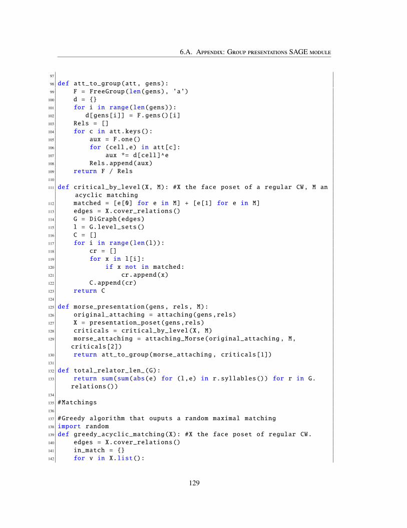
6.A. Appendix: Group presentations SAGE module

97

98 def att_to_group(att, gens):99 F = FreeGroup(len(gens), ’a’)

100 d = {}101 for i in range(len(gens)):102 d[gens[i]] = F.gens()[i]103 Rels = []104 for c in att.keys():105 aux = F.one()106 for (cell,e) in att[c]:107 aux *= d[cell]^e108 Rels.append(aux)109 return F / Rels110

111 def critical_by_level(X, M): #X the face poset of a regular CW, M anacyclic matching

112 matched = [e[0] for e in M] + [e[1] for e in M]113 edges = X.cover_relations()114 G = DiGraph(edges)115 l = G.level_sets()116 C = []117 for i in range(len(l)):118 cr = []119 for x in l[i]:120 if x not in matched:121 cr.append(x)122 C.append(cr)123 return C124

125 def morse_presentation(gens, rels, M):126 original_attaching = attaching(gens,rels)127 X = presentation_poset(gens,rels)128 criticals = critical_by_level(X, M)129 morse_attaching = attaching_Morse(original_attaching , M,

criticals[2])130 return att_to_group(morse_attaching , criticals[1])131

132 def total_relator_len_(G):133 return sum(sum(abs(e) for (l,e) in r.syllables()) for r in G.

relations())134

135 #Matchings136

137 #Greedy algorithm that ouputs a random maximal matching138 import random139 def greedy_acyclic_matching(X): #X the face poset of regular CW.140 edges = X.cover_relations()141 in_match = {}142 for v in X.list():

129

Chapter 6. New combinatorial methods for group presentations

143 in_match[v] = False144 seed()145 shuffle(edges)146 M = []147 for e in available_edges:148 if(in_match[e[0]] or in_match[e[1]]):149 continue150 D = DiGraph(edges)151 D.reverse_edge(e)152

153 if D.is_directed_acyclic():154 edges.remove(e)155 edges.append([e[1], e[0]])156 M.append(e)157 in_match[e[0]] = True158 in_match[e[1]] = True159 return M160

161 def spanning_matching(X):162 M = []163 n = 0164 while n != 1:165 M = greedy_acyclic_matching(X)166 n = len(critical_by_level(X, M)[0]) == 1167 return M168

130

Resumen del capítulo 6: Nuevos métodos combinatorios para pre-sentaciones de grupos

En este capítulo, realizamos un ataque combinatorio de la versión para presentaciones de gru-pos de la conjetura de Andrews-Curtis.

Dada una presentación P del grupo G, definimos XP, el poset asociado a la presentaciónP, como el face poset de la subdivisión baricéntrica de KP. Este poset tiene claramente sugrupo fundamental isomorfo a G, y su diagrama de Hasse puede ser descripto fácilmente entérminos de P. Sirve como modelo finito para estudiar su clase de Andrews-Curtis.

Proposición 6.1.4. Sean P,Q dos presentaciones de un grupo. Entonces,

(i) P ∼AC Q si y sólo si XP �↘3 XQ .

(ii) P es balanceada y G es el grupo trivial si y sólo si XP es homotópicamente trivial.

Dada una presentación balanceada del grupo trivial, elaboramos dos técnicas para transfor-marla en una nueva presentación en la misma clase de Andrews-Curtis, sin explicitar la lista demovimientos que llevan de una a la otra.

La primer técnica está inspirada en la teoría de coloreo de posets. Es una generalización eimplementación discreta del hecho de que colapsar un árbol en el 1-esqueleto de un 2-complejocelular es una 3-deformación.

Dado X un espacio finito de altura 2 y C un coloreo de X, definimos una presentación PX,C .

Definición 6.2.1. Sea X un espacio finito de altura 2 y sea C un subdiagrama de H(X). Lla-mamos a C un coloreo de H(X). Decimos que (x, y) es un par extremal de X si x < y,h(x) = 0, h(y) = 2. Para cada par extremal (x, y) de X, fijar, si es posible, una cadena pref-erencial cx,y : x ≺ z ≺ y tal que al menos uno de sus aristas no pertenece a C. Asociamosa (X,C) una presentación PX,C cuyos generadores son las aristas de H(X) que no pertenecena C, y cuyas relaciones están dadas por los rombos (i.e. pares de caminos monótonos que seintersecan en sus extremos) que contienen una cadena preferencial y no están completamentecoloreados por C.

Dado un espacio finito X de altura 2, vimos que si C ⊆ H(X) es un árbol o un subdiagramacolapsable con todos los vértices de X, entonces las distintas presentaciones PX,C pertenecena la misma clase de equivalencia de Andrews-Curtis. La llamamos PX cuando no queremosespecificar el subdiagrama C.

Teorema 6.2.6. Sean X,Y espacios finitos de altura 2. Entonces,

(i) X �↘3 Y si y sólo si PX ∼AC PY ;

(ii) X es homotópicamente trivial si y sólo si PX es una presentación balanceada del grupotrivial.

Teorema 6.3.1. SiP es una presentación de grupo y A es un subdiagrama generador colapsabledeH(XP), entonces P ∼AC PXP,A.

131

Capitulo 6: Nuevos metodos combinatorios para presentaciones de grupos

La otra técnica está inspirada en la teoría de Morse discreta, introducida por Robin Forman[For98] en los ’90s como una versión combinatoria de la teoría clásica para variedades diferen-ciables. Probamos una versión más fuerte del clásico teorema de Morse. Para lograrlo, hicimosuna reinterpretación del complejo de Morse en términos de colapsos internos.

Teorema 6.4.9. Sea K∪N⋃

i=1

ei un complejo celular, con K un subcomplejo de dimensión menos

o igual que k, tal que k ≤ dim(ei) ≤ dim(ei+1) para todo i. Denotamos por ϕ j : ∂D j → K∪⋃i< j

ei

a la función de adjunción de e j. Si K↘ L,

K ∪N⋃

i=1

ei �↘n+1

L ∪N⋃

i=1

ei

con n = dim(eN) y ϕ j : ∂D j → L∪⋃

i< j ei la función de adjunción de e j definida inductivamentepor ϕ1 = rϕ1 y si j > 1, ϕ j = f jϕ j, donde r : K → L es un retracto por deformación fuerte yf j : K ∪

⋃i< j

ei → L ∪⋃i< j

ei es una deformación.

En las hipótesis del teorema anterior, decimos que hay un colapso interno de K ∪⋃N

i=1 ei aL ∪

⋃Ni=1 ei.

Dado K un complejo celular regular de dimensión n y M un matching acíclico enH(X(K)),sabemos por el teorema de Morse que K tiene el mismo tipo homotópico que KM, un complejocon tantas celdas de dimensión k como celdas críticas en M de esa dimensión. Nosotros lo-gramos describir explícitamente a KM como el resultado de aplicarle a K una sucesión decolapsos internos determinados por M.

Teorema 6.4.17. Sea K un complejo celular regular de dimensión n sea M un matching acíclicoenH(X(K)). Entonces K �↘

n+1KM.

Dimos una descripción explícita de la presentación estándar asociada a KM, que denotamospor QX(K),M.

Definición 6.5.4. Sea K un complejo celular regular de dimensión 2. Sea M un matching enH(X(K)) tal que hay una sola celda crítica de dimensión 0. Denotamos por M0 al subconjuntode pares de puntos emparejados de alturas 0 y 1, y por Mr = {(x1, y1), (x2, y2), · · · , (xr, yr)} alsubconjunto se pares emparejados a alturas 1 y 2. Sea L un orden topológico preferencial deHM(X(K)). Ordenar Mk respecto de L, es decir, Mk = y1 < x1 < y2 < x2 < · · · < yr < xr,con (xi, yi) ∈ M. La presentación de grupo QX(K),M asociada al matching M es Qr definidainductivamente por:

• Q0 es la presentación estándar PK construida usando el spanning tree T inducido porM0. Las relaciones de Q0 con las 1-celdas de K no emparejadas según el matching M0, ysus relaciones son las palabras inducidas por las funciones de adjunción de las 2-celdasde K.

132

• Para 0 ≤ i < r, definimos Qi+1 como la presentación que se obtiene de Qi después deeliminar la relación asociada a yr−i y el generador xr−i, y reemplazar cada ocurrencia delgenerador xr−i en los restantes generadores por la expresión equivalente de xr−i inferidapor la relación asociada a yr−i.

Corolario 6.5.6. Sea K un complejo celular regular de dimensión 2, y sea M un matchingacíclico en H(X(K)) con una sola celda crítica de dimensión 0. Entonces, QX(K),M es unapresentación balanceada de π1(K) . Más aún, QX(K),M ∼AC PK .

Usando los métodos anteriores, implementamos en SAGE algoritmos concretos para obtenerpresentaciones AC-equivalentes a una presentación dada, sin necesidad de explicitar la lista demovimientos de Andrews-Curtis que llevan de una a la otra.

Obtuvimos, entre otras, demostraciones experimentales simples de los siguientes hechossobre la lista de potenciales contraejemplos.

• La presentación 〈x, y | xyx = yxy, xn = yn+1〉 [AK85] para n = 2, satisface la conjeturade Andrews-Curtis.

• La presentación 〈x, y, z | z−1yz = y2, x−1zx = z2, y−1xy = x2〉 [Rap68a], se puede trasfor-mar en una presentación con 2 generadores y 2 relaciones.

• Hay una gran clase de enteros n,m, p, q para la cual la presentación 〈x, y | x = [xm, yn], y =

[xp, yq]〉 [Bro84] satisface la conjetura. 3.

No se conocía si en general las presentaciones de esta familia satisfacen la conjetura deAndrews-Curtis. Sin embargo, algunas de ellas pueden probarse AC-tivializables usandola rutina simplified.

Nosotros probamos experimentalmente que las presnetacioens

G1,1,k,−1 = 〈x, y | x = [x, y], y = [xp, y−1]〉

for 1 ≤ p ≤ 100 satisfacen la conjetura. Si k es impar, la rutina simplified alcanza,pero si k es par, no. Nosotros logramos hallar, para cada k, un matching acíclico Mk

en H(XG1,1,k,−1) tan que QXG1,1,k,−1 ,Mk se puede reducir a la presentación trivial del grupotrivial luego de aplicar la función simplified.

3Aquí, [a, b] = a−1b−1ab.

133

Capitulo 6: Nuevos metodos combinatorios para presentaciones de grupos

134

Bibliography

[AC65] J. J. Andrews and M. L. Curtis. Free groups and handlebodies. Proc. Amer. Math.Soc., 16:192–195, 1965.

[AC66] J. J. Andrews and M. L. Curtis. Extended Nielsen operations in free groups. Amer.Math. Monthly, 73:21–28, 1966.

[Adi93] S. I. Adian. On some algorithmic problems for groups and monoids. In Rewritingtechniques and applications (Montreal, PQ, 1993), volume 690 of Lecture Notesin Comput. Sci., pages 289–300. Springer, Berlin, 1993.

[AK85] S. Akbulut and R. Kirby. A potential smooth counterexample in dimension 4to the Poincaré conjecture, the Schoenflies conjecture, and the Andrews-Curtisconjecture. Topology, 24(4):375–390, 1985.

[Ale37] P. Alexandroff. Diskrete raüme. MathematiceskiiSbornik (N.S.), 2(3):501–518,1937.

[Bar11a] J. A. Barmak. Algebraic topology of finite topological spaces and applications,volume 2032 of Lecture Notes in Mathematics. Springer, Heidelberg, 2011.

[Bar11b] J. A. Barmak. On Quillen’s Theorem A for posets. J. Combin. Theory Ser. A,118(8):2445–2453, 2011.

[BEJM15] P. Brendel, G. Ellis, M. Juda, and M. Mrozek. Fundamental Group Algorithm forlow dimensional tessellated CW complexes. ArXiv e-prints, July 2015.

[Bj"03] A. Bj"orner. Nerves, fibers and homotopy groups. J. Combin. Theory Ser. A,102(1):88–93, 2003.

[BK72] A. K. Bousfield and D. M. Kan. Homotopy limits, completions and localizations.Lecture Notes in Mathematics, Vol. 304. Springer-Verlag, Berlin-New York, 1972.

[BM06] R. S. Bowman and S. B. McCaul. Fast searching for Andrews-Curtis trivializa-tions. Experiment. Math., 15(2):193–197, 2006.

[BM07] J. A. Barmak and E. G. Minian. Minimal finite models. J. Homotopy Relat. Struct.,2(1):127–140, 2007.

135

Bibliography

[BM08a] J. A. Barmak and E. G. Minian. One-point reductions of finite spaces, h-regularCW-complexes and collapsibility. Algebr. Geom. Topol., 8(3):1763–1780, 2008.

[BM08b] J. A. Barmak and E. G. Minian. Simple homotopy types and finite spaces. Adv.Math., 218(1):87–104, 2008.

[BM12a] J. A. Barmak and E. G. Minian. G-colorings of posets, coverings and presentationsof the fundamental group. ArXiv e-prints, December 2012.

[BM12b] J. A. Barmak and E. G. Minian. Strong homotopy types, nerves and collapses.Discrete Comput. Geom., 47(2):301–328, 2012.

[Boo54a] W. W. Boone. Certain simple, unsolvable problems of group theory. I. Nederl.Akad. Wetensch. Proc. Ser. A., 57:231–237 = Indag. Math. 16, 231–237 (1954),1954.

[Boo54b] W. W. Boone. Certain simple, unsolvable problems of group theory. II. Nederl.Akad. Wetensch. Proc. Ser. A., 57:492–497 = Indag. Math. 16, 492–497 (1954),1954.

[Boo55a] W. W. Boone. Certain simple, unsolvable problems of group theory. III. Nederl.Akad. Wetensch. Proc. Ser. A., 58:252–256 = Indag. Math. 17, 252–256 (1955),1955.

[Boo55b] W. W. Boone. Certain simple, unsolvable problems of group theory. IV. Nederl.Akad. Wetensch. Proc. Ser. A. 58 = Indag. Math., 17:571–577, 1955.

[Bor48] K. Borsuk. On the imbedding of systems of compacta in simplicial complexes.Fund. Math., 35:217–234, 1948.

[Bri15] M. R. Bridson. The complexity of balanced presentations and the andrews-curtisconjecture. arXiv preprint arXiv:1504.04187, 2015.

[Bro84] R. Brown. Coproducts of crossed P-modules: applications to second homotopygroups and to the homology of groups. Topology, 23(3):337–345, 1984.

[BWW05] A. Björner, M. L. Wachs, and V. Welker. Poset fiber theorems. Trans. Amer. Math.Soc., 357(5):1877–1899, 2005.

[CF77] R. H. Crowell and R. H. Fox. Introduction to knot theory. Springer-Verlag, NewYork-Heidelberg, 1977. Reprint of the 1963 original, Graduate Texts in Mathe-matics, No. 57.

[Cha00] M. K. Chari. On discrete Morse functions and combinatorial decompositions.Discrete Math., 217(1-3):101–113, 2000. Formal power series and algebraic com-binatorics (Vienna, 1997).

[Coh67] M. M. Cohen. Simplicial structures and transverse cellularity. Ann. of Math. (2),85:218–245, 1967.

136

Bibliography

[Coh69] M. M. Cohen. A general theory of relative regular neighborhoods. Trans. Amer.Math. Soc., 136:189–229, 1969.

[Coh73] M. M. Cohen. A course in simple-homotopy theory. Springer-Verlag, New York-Berlin, 1973. Graduate Texts in Mathematics, Vol. 10.

[Deh11] M. Dehn. Über unendliche diskontinuierliche Gruppen. Math. Ann., 71(1):116–144, 1911.

[Deh12] M. Dehn. Transformation der Kurven auf zweiseitigen Flächen. Math. Ann.,72(3):413–421, 1912.

[Fer11] X. L. Fernández. Espacios topológicos finitos: un enfoque algorítmico. Mas-ter’s thesis, Departamento de Matemática. Universidad de Buenos Aires, xfer-nand@dm.uba.ar, 3 2011.

[Fer17] X. L. Fernández. Some topological algorithms on the Andrews-Curtis conjecture.Work in progress, 2017.

[FM16] X. L. Fernández and E. G. Minian. Homotopy colimits of diagrams over posets andvariations on a theorem of Thomason. Homology Homotopy Appl., 18(2):233–245,2016.

[FM17] X. L. Fernández and E. G. Minian. The cylinder of a relation and 3-deformations.Preprint, 2017.

[For98] R. Forman. Morse theory for cell complexes. Adv. Math., 134(1):90–145, 1998.

[For02] R. Forman. A user’s guide to discrete Morse theory. Sém. Lothar. Combin., 48:Art.B48c, 35, 2002.

[Gad01] S. Gadgil. On the andrews-curtis conjecture and algorithms from topology. arXivpreprint math/0108053, 2001.

[GAP17] The GAP Group. GAP – Groups, Algorithms, and Programming, Version 4.8.7,2017.

[GR83] D. Gillman and D. Rolfsen. The Zeeman conjecture for standard spines is equiva-lent to the Poincaré conjecture. Topology, 22(3):315–323, 1983.

[HAM90] C. Hog-Angeloni and W. Metzler. Stabilization by free products giving rise toandrews-curtis equivalences. Note di Matematica, 10(suppl. 2):305–314, 1990.

[HAM93] C. Hog-Angeloni and W. Metzler, editors. Two-dimensional homotopy and combi-natorial group theory, volume 197 of London Mathematical Society Lecture NoteSeries. Cambridge University Press, Cambridge, 1993.

[Hat02] A. Hatcher. Algebraic topology. Cambridge University Press, Cambridge, 2002.

137

Bibliography

[HKRR84] G. Havas, P. E. Kenne, J. S. Richardson, and E. F. Robertson. A Tietze transfor-mation program. In Computational group theory (Durham, 1982), pages 69–73.Academic Press, London, 1984.

[HR03] G. Havas and C. Ramsay. Breadth-first search and the Andrews-Curtis conjecture.Internat. J. Algebra Comput., 13(1):61–68, 2003.

[Hud69] J. F. P. Hudson. Piecewise linear topology. University of Chicago Lecture Notesprepared with the assistance of J. L. Shaneson and J. Lees. W. A. Benjamin, Inc.,New York-Amsterdam, 1969.

[Koz08] D. Kozlov. Combinatorial algebraic topology, volume 21 of Algorithms and Com-putation in Mathematics. Springer, Berlin, 2008.

[Ler45] J. Leray. Sur la forme des espaces topologiques et sur les points fixes des représen-tations. J. Math. Pures Appl. (9), 24:95–167, 1945.

[LS01] R. C. Lyndon and P. E. Schupp. Combinatorial group theory. Classics in Mathe-matics. Springer-Verlag, Berlin, 2001. Reprint of the 1977 edition.

[May12] J. P. May. Finite spaces and larger contexts. book draft downloaded from, pages12–14, 2012.

[McC66] M. C. McCord. Singular homology groups and homotopy groups of finite topo-logical spaces. Duke Math. J., 33:465–474, 1966.

[Met79] W. Metzler. Äquivalenzklassen von Gruppenbeschreibungen, Identitäten und ein-facher Homotopietyp in niederen Dimensionen. In Homological group theory(Proc. Sympos., Durham, 1977), volume 36 of London Math. Soc. Lecture NoteSer., pages 291–326. Cambridge Univ. Press, Cambridge-New York, 1979.

[Mia99] A. D. Miasnikov. Genetic algorithms and the Andrews-Curtis conjecture. Internat.J. Algebra Comput., 9(6):671–686, 1999.

[Mil59] J. Milnor. On spaces having the homotopy type of a CW-complex. Trans. Amer.Math. Soc., 90:272–280, 1959.

[Mil66] J. Milnor. Whitehead torsion. Bull. Amer. Math. Soc., 72:358–426, 1966.

[MM01] A. D. Miasnikov and A. G. Myasnikov. Balanced presentations of the trivial groupon two generators and the Andrews-Curtis conjecture. In Groups and computation,III (Columbus, OH, 1999), volume 8 of Ohio State Univ. Math. Res. Inst. Publ.,pages 257–263. de Gruyter, Berlin, 2001.

[Moi77] E. E. Moise. Geometric topology in dimensions 2 and 3. Springer-Verlag, NewYork-Heidelberg, 1977. Graduate Texts in Mathematics, Vol. 47.

[MS99] C. F. Miller, III and P. E. Schupp. Some presentations of the trivial group. InGroups, languages and geometry (South Hadley, MA, 1998), volume 250 of Con-temp. Math., pages 113–115. Amer. Math. Soc., Providence, RI, 1999.

138

Bibliography

[Nie18] J. Nielsen. über die Isomorphismen unendlicher Gruppen ohne Relation. Math.Ann., 79(3):269–272, 1918.

[Nov55] P. S. Novikov. Ob algoritmiceskoı nerazrešimosti problemy toždestva slov v teoriigrupp. Trudy Mat. Inst. im. Steklov. no. 44. Izdat. Akad. Nauk SSSR, Moscow,1955.

[Osa99] T. Osaki. Reduction of finite topological spaces. Interdiscip. Inform. Sci.,5(2):149–155, 1999.

[Per02] G. Perelman. The entropy formula for the ricci flow and its geometric applications.arXiv preprint math/0211159, 2002.

[Per03a] G. Perelman. Finite extinction time for the solutions to the ricci flow on certainthree-manifolds. arXiv preprint math/0307245, 2003.

[Per03b] G. Perelman. Ricci flow with surgery on three-manifolds. arXiv preprintmath/0303109, 2003.

[Qui72] D. Quillen. Higher algebraic K-theory. I. pages 85–147. Lecture Notes in Math.,Vol. 341, 1972.

[Qui78] D. Quillen. Homotopy properties of the poset of nontrivial p-subgroups of a group.Adv. in Math., 28(2):101–128, 1978.

[Rab58] M. O. Rabin. Recursive unsolvability of group theoretic problems. Ann. of Math.(2), 67:172–194, 1958.

[Rap68a] E. S. Rapaport. Groups of order 1: Some properties of presentations. Acta Math.,121:127–150, 1968.

[Rap68b] E. S. Rapaport. Remarks on groups of order 1. Amer. Math. Monthly, 75:714–720,1968.

[RS72] C. P. Rourke and B. J. Sanderson. Introduction to piecewise-linear topology.Springer-Verlag, New York-Heidelberg, 1972. Ergebnisse der Mathematik undihrer Grenzgebiete, Band 69.

[S+17] W. A. Stein et al. Sage Mathematics Software (Version x.y.z). The Sage Develop-ment Team, 2017. http://www.sagemath.org.

[Seg68] G. Segal. Classifying spaces and spectral sequences. Inst. Hautes Études Sci. Publ.Math., (34):105–112, 1968.

[Sto66] R. E. Stong. Finite topological spaces. Trans. Amer. Math. Soc., 123:325–340,1966.

[tD71] T. tom Dieck. Partitions of unity in homotopy theory. Composito Math., 23:159–167, 1971.

139

Bibliography

[Tho79] R. W. Thomason. Homotopy colimits in the category of small categories. Math.Proc. Cambridge Philos. Soc., 85(1):91–109, 1979.

[Tie08] H. Tietze. Über die topologischen Invarianten mehrdimensionaler Mannig-faltigkeiten. Monatsh. Math. Phys., 19(1):1–118, 1908.

[Tur37] A. M. Turing. On computable numbers, with an application to the entschei-dungsproblem. Proceedings of the London mathematical society, 2(1):230–265,1937.

[Vog73] R. M. Vogt. Homotopy limits and colimits. pages 235–241, 1973.

[Wal65] C. T. C. Wall. Finiteness conditions for CW-complexes. Ann. of Math. (2), 81:56–69, 1965.

[Wal66a] C. T. C. Wall. Finiteness conditions for CW complexes. II. Proc. Roy. Soc. Ser. A,295:129–139, 1966.

[Wal66b] C. T. C. Wall. Formal deformations. Proc. London Math. Soc. (3), 16:342–352,1966.

[Whi39] J. H. C. Whitehead. Simplicial Spaces, Nuclei and m-Groups. Proc. London Math.Soc., S2-45(1):243, 1939.

[Whi41a] J. H. C. Whitehead. On adding relations to homotopy groups. Ann. of Math. (2),42:409–428, 1941.

[Whi41b] J. H. C. Whitehead. On incidence matrices, nuclei and homotopy types. Ann. ofMath. (2), 42:1197–1239, 1941.

[Whi49] J. H. C. Whitehead. Combinatorial homotopy. I. Bull. Amer. Math. Soc., 55:213–245, 1949.

[Whi50] J. H. C. Whitehead. Simple homotopy types. Amer. J. Math., 72:1–57, 1950.

[Wri75] P. Wright. Group presentations and formal deformations. Trans. Amer. Math. Soc.,208:161–169, 1975.

[WZv99] V. Welker, G. M. Ziegler, and R. T. Živaljevic. Homotopy colimits—comparisonlemmas for combinatorial applications. J. Reine Angew. Math., 509:117–149,1999.

[Zee64] E. C. Zeeman. On the dunce hat. Topology, 2:341–358, 1964.

[Zv93] G. M. Ziegler and R. T. Živaljevic. Homotopy types of subspace arrangements viadiagrams of spaces. Math. Ann., 295(3):527–548, 1993.

140