revisión bibliográfica de problemas combinatorios

Ouafae Debdi J. Ángel Velázquez Iturbide Maximiliano Paredes Velasco

Revisión Bibliográfica de Problemas Combinatorios Resolubles por Técnicas Básicas de Diseño de Algoritmos Número 2010-03 Serie de Informes Técnicos DLSI1-URJC ISSN 1988-8074 Departamento de Lenguajes y Sistemas Informáticos I Universidad Rey Juan Carlos

Índice

1 Introducción............................................................................................................. 1 2 Problemas de planificación...................................................................................... 3

2.1 Grupo 1 ............................................................................................................ 3 2.2 Grupo 2: Problemas de la mochila ................................................................... 4 2.3 Grupo 3 ............................................................................................................ 7 2.4 Grupo 4 .......................................................................................................... 10 2.5 Grupo 5: Planificación con plazo fijo ............................................................ 12 2.6 Grupo 6: Selección de actividades ................................................................. 16 2.7 Grupo 7 .......................................................................................................... 18 2.8 Agrupamiento de problemas .......................................................................... 24

3 Problemas de monedas .......................................................................................... 26 3.1 Problema del cambio de monedas.................................................................. 26 3.2 Problemas relacionados.................................................................................. 26

4 Problemas de mezcla de cintas .............................................................................. 29 5 Problemas de cadenas de caracteres ...................................................................... 31

5.1 La subsecuencia común más larga ................................................................. 31 5.2 Otros problemas de cadenas de caracteres ..................................................... 31

6 Problemas de multiplicación de matrices .............................................................. 38 6.1 Multiplicación encadenada de matrices ......................................................... 38 6.2 Problemas relacionados.................................................................................. 39

7 Códigos de Huffman............................................................................................. 40 8 Problema del árbol de recubrimiento del coste mínimo......................................... 41 9 Problemas de caminos más cortos ......................................................................... 43

9.1 Problema del camino más corto desde un origen........................................... 43 9.2 Problema del camino más corto entre todos los pares de nodos .................... 44 9.3 Problemas relacionados.................................................................................. 45

10 Problemas de grafos............................................................................................. 46 11 Otros problemas................................................................................................... 55 12 Conclusiones........................................................................................................ 60 Referencias ................................................................................................................. 60

Revisión Bibliográfica de Problemas Combinatorios Resolubles por Técnicas Básicas de Diseño de Algoritmos

Ouafae Debdi, J. Ángel Velázquez Iturbide, Maximiliano Paredes Velasco

Departamento de Lenguajes y Sistemas Informáticos I, Universidad Rey Juan Carlos, C/ Tulipán s/n, 28933, Móstoles, Madrid

{ouafae.debdi,angel.velazquez,maximiliano.paredes}@urjc.es

Abstract. Existen varios tipos de problemas que se puedan resolver aplicando un algoritmo u otro, el siguiente trabajo recopila y recoge desde varios libros de texto los diferentes tipos de problemas que se pueden solucionar mediante algoritmos voraces, algoritmos aproximados (y heurísticas) y algoritmos de programación dinámica, llegando a una revisión bibliografiíta que organiza y agrupa los diferentes tipos de problemas.

Keywords: problemas combinatorios, programación dinámica, algoritmos voraces, algoritmos aproximados y heurísticas.

1 Introducción

El presente trabajo recoge y recopila numerosos problemas combinatorios que se pueden resolver mediante las técnicas de algoritmos voraces, algoritmos aproximados (o heurísticos) o programación dinámica.

La recopilación se ha realizado a partir de 14 libros de texto prestigiosos sobre algoritmos [1-14]. No definimos aquí ninguna de las técnicas de diseño anteriores, ya que pueden encontrarse en casi todos los libros citados.

La búsqueda se ha realizado en cada libro siguiendo el siguiente procedimiento. Primero, se ha buscado en el índice del libro si había algún capítulo sobre cada técnica de diseño. En caso afirmativo, se ha realizado la búsqueda en el mismo; si no, se ha buscado en el glosario de términos el nombre de problemas conocidos (por ejemplo, algoritmo de Dijkstra, problema de la mochila, etc.).

El objetivo del trabajo es múltiple: • Recopilar una parte importante de la gran variedad de problemas combinatorios

utilizados en los libros de texto para ilustrar las técnicas de diseño de algoritmos mencionadas. Este objetivo es de interés para profesores o investigadores de algoritmos.

• Explorar la posibilidad de generalizar la forma de organizar los problemas sobre estas técnicas. Este objetivo es de interés para la línea de investigación que tenemos abierta sobre diseño de ayudantes interactivos para el aprendizaje de algoritmos voraces [15,16].

2

El informe presenta los problemas organizados en 10 grupos: 1. Problemas de planificación. 2. Problemas de monedas. 3. Problemas de mezcla de cintas. 4. Problemas de cadenas de caracteres. 5. Problemas de multiplicación de matrices. 6. Códigos de Huffman. 7. Problema del árbol de recubrimiento de coste mínimo. 8. Problemas de caminos de coste mínimo. 9. Otros problemas de grafos. 10. Otros problemas.

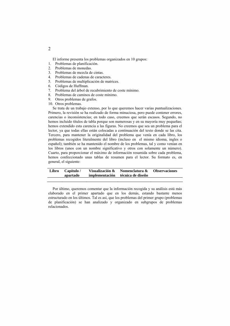
Se trata de un trabajo extenso, por lo que queremos hacer varias puntualizaciones. Primero, la revisión se ha realizado de forma minuciosa, pero puede contener errores, carencias o inconsistencias; en todo caso, creemos que serán escasos. Segundo, no hemos incluido títulos de tabla porque son numerosas y en su mayoría muy pequeñas; hemos extendido esta carencia a las figuras. No creemos que sea un problema para el lector, ya que todas ellas están colocadas a continuación del texto donde se las cita. Tercero, para mantener la originalidad del problema que venía en cada libro, los problemas recogidos literalmente del libro (incluso en el mismo idioma, ingles o español); también se ha mantenido el nombre de los problemas, tal y como venían en los libros (unos con un nombre significativo y otros con solamente un número). Cuarto, para proporcionar el máximo de información resumida sobre cada problema, hemos confeccionado unas tablas de resumen para el lector. Su formato es, en general, el siguiente:

Libro Capítulo /

apartado Visualización & implementación

Nomenclatura & técnica de diseño

Observaciones

Por último, queremos comentar que la información recogida y su análisis está más

elaborado en el primer apartado que en los demás, estando bastante menos estructurado en los últimos. Tal es así, que los problemas del primer grupo (problemas de planificación) se han analizado y organizado en subgrupos de problemas relacionados.

3

2 Problemas de planificación

En este apartado veremos un gran número de problemas distintos, aunque con algo en común: hay que planificar el uso de ciertos recursos. Comenzamos presentándolos por categorías; esta agrupación es relativamente arbitraria, pero nos facilita el estudio de ellos. En el subapartado 0 se agrupan de una forma más razonada.

2.1 Grupo 1

Problema 1. Maximum programs stored problem Assume that we have n programs and two storage devices (say disks or tapes). We shall assume the devices are disks. Our discussion applies to any kind of storage device. Let li be the amount of storage needed to store the ith program. Let L be the storage capacity of each disk. Determining the maximum number of these n programs that can be stored on the two disks (without splitting a program over the disks) is NP-hard.

Libro Capítulo / apartado

Visualización & implementación

Técnica de diseño Observaciones

E. Horowitz y S. Sahni, Fundamentals of Computer Algorithms

Capítulo 12 Apartado 2

Algoritmo p. 564 Approximation algorithms −

Problema de maximización de programas en un disco Consideramos n programas p1, p2,.., pn que debemos almacenar en un disco. El programa pi requiere si megabytes de espacio de disco, y la capacidad del disco es D megabytes. (a) Problema 2. Se desea maximizar el número de programas almacenados en el

disco. Demostrar lo siguiente o dar un contraejemplo: podemos utilizar un algoritmo voraz que seleccione los programas por orden creciente de si.

N. Martí Oliet, Y. Ortega y J.A. Verdejo, Estructuras de datos y métodos algorítmicos: ejercicios resueltos


Algoritmo p. 357 Método voraz Demostración de optimidad (reducción de diferencias)

S. Sahni, Data Structures, Algorihtms and Applications in Java


Implementación p. 709

Greedy method Análisis de complejidad

(b) Problema 3. Se desea maximizar el espacio utilizado del disco. Demostrar lo

siguiente o dar un contraejemplo: se puede utilizar un algoritmo voraz que seleccione los programas por orden decreciente de si.

4






− Método voraz Contrajemplo

Problema 2. Loading problem (container loading) A large ship is to be loaded with cargo. The cargo is containerized, and all containers are the same size. Different containers may have different weights. Let wi be the weight of the ith container, 1≤i≤n. The cargo capacity of the ship is c. We wish to load the ship with the maximum number of containers.

This problem can be formulated as an optimization problem in the following way: Let xi be a variable whose value can be either 0 or 1. If we set xi to 0, then container i is not to be loaded. If xi is 1, then the container is to be loaded. We wish to assign

values to the xis that satisfy the constraints cxw in

i i ≤∑ =1and }{ nixi ≤≤∈ 1,1,0 .

The optimization function is∑ =

n

i ix1

.

Every set of xi’s that satisfies the constraints is a feasible solution. Every feasible

solution that maximizes ∑ =

n

i ix1

is an optimal solution.

The ship may be loaded in stages; one container per stage. At each stage we need to decide which container to load. For this decision we may use the greedy criterion: from the remaining containers, select the one with least weight. This order of selection will keep the total weight of the selected containers minimum and hence leave maximum capacity for loading more containers. Using the greedy algorithm just outlined, we first select the container that has least weight, then the one with the next smallest weight, and so on until either all containers have been loaded or there isn’t enough capacity for the next one. Example: Suppose that n=8, [w1,…,w8]=[100,200,50,90,150,50,20,80], and c=400. When the greedy algorithm is used, the containers are considered for loading in the order 7,3,6,8,4,1,5,2. Containers 7,3,6,8,4, and 1 together weigh 390 units and are loaded. The available capacity is now 10 units, which is inadequate for any of the remaining containers.

In the greedy solution we have [x1,…,x8]=[1,0,1,1,0,1,1,1] and ∑xi=6

2.2 Grupo 2: Problemas de la mochila

Sean n objetos y una mochila. Cada objeto i, 1≤i≤n, tiene un peso positivo pi. Si se introduce en la mochila, produce un valor positivo o beneficio bi. La mochila puede llevar un peso que no sobrepase w.

Nuestro objetivo es llenar la mochila de tal manera que se maximice el beneficio producido por los objetos introducidos respetando la limitación de capacidad impuesta.

5

Por ejemplo, supongamos que están disponibles tres objetos, el primero de los cuales pesa 6 unidades y tiene un valor de 8, mientras que los otros dos pesan 5 unidades cada uno y tienen un valor de 5 cada uno. Si la mochila puede llevar 10 unidades, entonces la carga óptima incluye a los dos objetos más ligeros, con un valor total de 10. El algoritmo voraz, por otra parte, comenzaría por seleccionar el objeto que pesa 6 unidades, puesto que es el que tiene un mayor valor por unidad de peso. Sin embargo, si los objetos no se pueden romper, el algoritmo no podrá utilizar la capacidad restante de la mochila. La carga que produce, por tanto, consta de un solo objeto, y tiene un valor de 8 nada más.

Existen dos variantes del problema de la mochila que son:

Problema 4. Problema de la mochila. Se pueden romper los objetos en trozos pequeños, de manera que podamos decidir llevar solamente una fracción xi.

Problema 5. Problema de la mochila 0/1. Los objetos no se pueden fragmentar en trozos pequeños, así que podemos decidir si tomamos un objeto o lo dejamos.




Observaciones

M.H. Alsuwaiyel, Algorithms Design Techniques and Analysis


Algoritmo p. 218 The knapsack problem – Dynamic programming

Análisis de complejidad

M.H. Alsuwaiyel, Algorithms Design Techniques and Analysis

Capítulo 15 Apartado 5.1

Algoritmo p. 405 The knapsack problem – Approximation algorithms


G. Brassard y P. Bratley, Fundamentos de algoritmia


Tabla p. 300 Mochila 0/1 (problema de la mochila) – Programación dinámica




Pseudocódigo p. 533

Mochila (problema de la mochila) – Algoritmo aproximado

Demostración de la eficacia del algoritmo aproximado




Mochila (problema de la mochila) – Algoritmo voraz


M.T. Goodrich y R. Tamassia, Data Structures and Algorithms in Java


Algoritmo p. 511 The fractional knapsack problem – The greedy method


M.T. Goodrich y R. Tamassia, Data Structures and Algorithms in Java


Algoritmo p. 509

The 0/1 knapsack problem – Dynamic programming


E. Horowitz y S. Sahni, Computer Algorithms


Pseudocódigo p. 223 Figura y código

The 0/1 knapsack – Dynamic programming





0/1 knapsack problem – Approximation algorithm





Knapsack problem – The greedy method


R.C.T. Lee, S.S. Tseng, R.C. Chang e Y.T. Tsai, Introducción al diseño y análisis de algoritmos


Pseudocódigo p.449-455

Problema 0/1 de la mochila – Algoritmos de aproximación


6



Figura p. 283 Problema 0/1 de la mochila – Programación dinámica

−


Capítulo 12 Apartado 5(a)

Pseudocódigos p. 362 y 363

(Alí Babá y los Cuarenta Ladrones) – Algoritmo voraz

Demostración de optimidad (reducción de diferencias) Análisis de complejidad


Capítulo 12 Apartado 5©

− (Alí Babá y los Cuarenta Ladrones) – Algoritmo voraz

Contraejemplo


Capítulo 13 Apartado 2(a)

Pseudocódigo p. 404 Figura tabla p. 404

(Alí Babá y los Cuarenta Ladrones) – Programación dinámica


R. Neapolitan y K. Naimipour, Foundations of Algorithms


Ejemplo y figura p. 167

The 0/1 knapsack problem – The greedy approach

Solución del ejemplo con �raccional knapsack problem



Ejemplo p. 169 The 0/1 knapsack problem – Dynamic programming


I. Parberry, Problems on Algorithms Capítulo 8 Apartado 2

Pseudocódigo p. 89

The knapsack problem – Dynamic programming

−



The knapsack problem – Greedy algorithms

−

S. Sahni, Data Structures, Algorithms, and Applications in Java


Ejemplos p. 711 0/1 knapsack problem – The greedy heuristics




Código recursivo p. 802 Código iterativo p. 804

0/1 knapsack problem – Dynamic programming

Análisis de complejidad de implementaciones recursiva e iterativa



Ejemplo p. 709 0/1 knapsack problem – The greedy method

Posibles estrategias voraces

R. Sedgewick, Algorithms in Java Capítulo 5 Apartado 12

Pseudocódigo p. 225 Solución recursiva Figuras

Knapsack problem – Dynamic programming

−

S. Skeina, The Algorithm Design Manual


Figuras p. 229 Knapsack problem – −

7

También se encuentran otros variantes, de las que algunas se presentan en la tabla siguiente.

Libro Capítulo /



Observaciones


Capítulo 12 Apartado 5©


(Alí Babá y los Cuarenta Ladrones) – Algoritmo voraz

Demostración de optimidad (reducción a problema) Análisis de complejidad


Capítulo 12 Apartado 5(d)

− (Alí Babá y los Cuarenta Ladrones) – Algoritmo voraz

−


Capítulo 13 Apartados 2(b) y 2(c)


(Alí Babá y los Cuarenta Ladrones) – Programación dinámica


2.3 Grupo 3

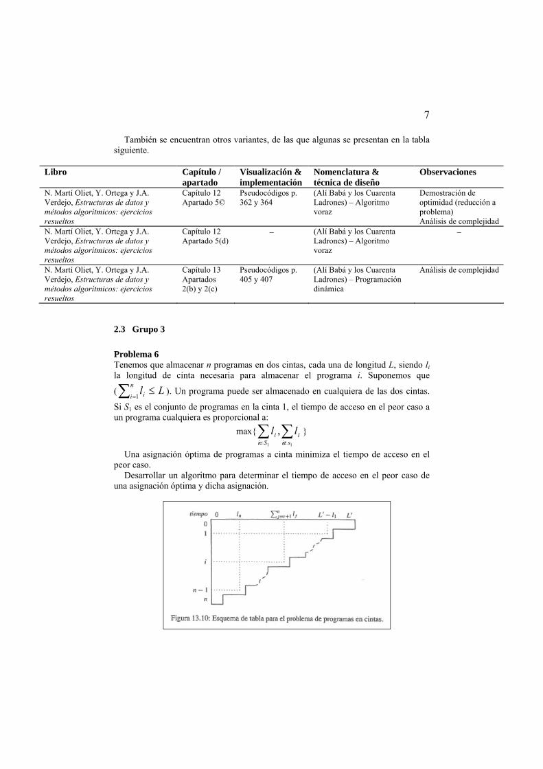
Problema 6 Tenemos que almacenar n programas en dos cintas, cada una de longitud L, siendo li la longitud de cinta necesaria para almacenar el programa i. Suponemos que

( Lln

i i ≤∑ =1). Un programa puede ser almacenado en cualquiera de las dos cintas.

Si S1 es el conjunto de programas en la cinta 1, el tiempo de acceso en el peor caso a un programa cualquiera es proporcional a:

max{ ∑∑∉∈ 11

,si

iSi

i ll }

Una asignación óptima de programas a cinta minimiza el tiempo de acceso en el peor caso.

Desarrollar un algoritmo para determinar el tiempo de acceso en el peor caso de una asignación óptima y dicha asignación.

8

Libro Capítulo /





Tres soluciones del problema Algoritmos p. 436, 437 y 438 Figura p. 436

Programación dinámica Análisis de complejidad

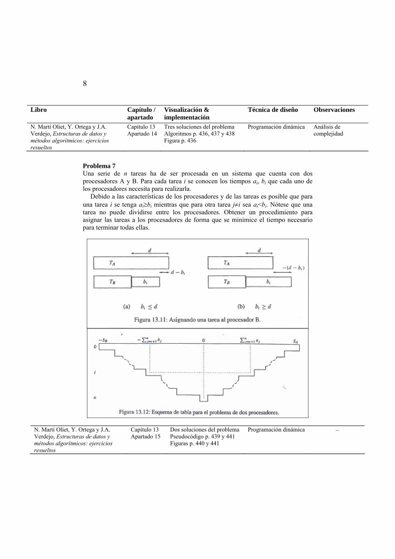
Problema 7 Una serie de n tareas ha de ser procesada en un sistema que cuenta con dos procesadores A y B. Para cada tarea i se conocen los tiempos ai, bi que cada uno de los procesadores necesita para realizarla.

Debido a las características de los procesadores y de las tareas es posible que para una tarea i se tenga ai≥bi mientras que para otra tarea j≠i sea ai<bi. Nótese que una tarea no puede dividirse entre los procesadores. Obtener un procedimiento para asignar las tareas a los procesadores de forma que se minimice el tiempo necesario para terminar todas ellas.



Dos soluciones del problema Pseudocódigo p. 439 y 441 Figuras p. 440 y 441

Programación dinámica −

9

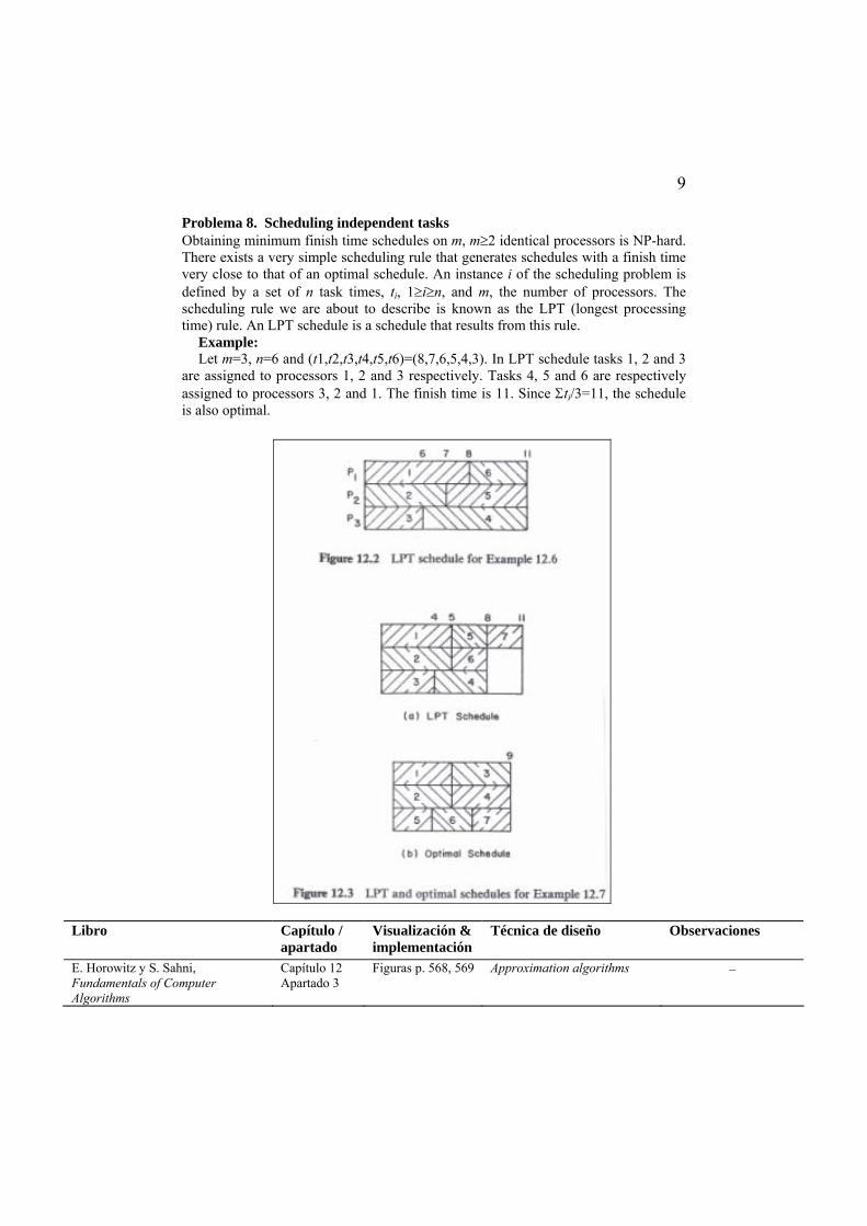
Problema 8. Scheduling independent tasks Obtaining minimum finish time schedules on m, m≥2 identical processors is NP-hard. There exists a very simple scheduling rule that generates schedules with a finish time very close to that of an optimal schedule. An instance i of the scheduling problem is defined by a set of n task times, ti, 1≥i≥n, and m, the number of processors. The scheduling rule we are about to describe is known as the LPT (longest processing time) rule. An LPT schedule is a schedule that results from this rule.

Example: Let m=3, n=6 and (t1,t2,t3,t4,t5,t6)=(8,7,6,5,4,3). In LPT schedule tasks 1, 2 and 3

are assigned to processors 1, 2 and 3 respectively. Tasks 4, 5 and 6 are respectively assigned to processors 3, 2 and 1. The finish time is 11. Since Σti/3=11, the schedule is also optimal.






Figuras p. 568, 569

Approximation algorithms −

10

2.4 Grupo 4

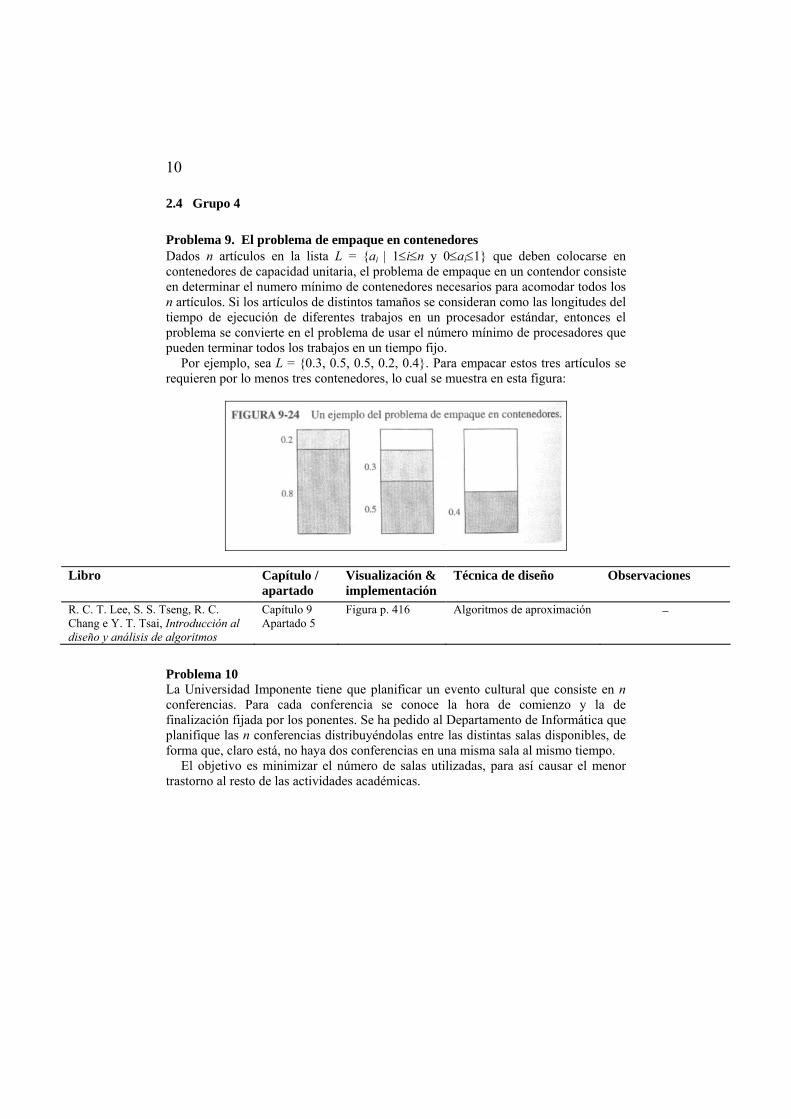
Problema 9. El problema de empaque en contenedores Dados n artículos en la lista L = {ai | 1≤i≤n y 0≤ai≤1} que deben colocarse en contenedores de capacidad unitaria, el problema de empaque en un contendor consiste en determinar el numero mínimo de contenedores necesarios para acomodar todos los n artículos. Si los artículos de distintos tamaños se consideran como las longitudes del tiempo de ejecución de diferentes trabajos en un procesador estándar, entonces el problema se convierte en el problema de usar el número mínimo de procesadores que pueden terminar todos los trabajos en un tiempo fijo.

Por ejemplo, sea L = {0.3, 0.5, 0.5, 0.2, 0.4}. Para empacar estos tres artículos se requieren por lo menos tres contenedores, lo cual se muestra en esta figura:




R. C. T. Lee, S. S. Tseng, R. C. Chang e Y. T. Tsai, Introducción al diseño y análisis de algoritmos


Figura p. 416 Algoritmos de aproximación −

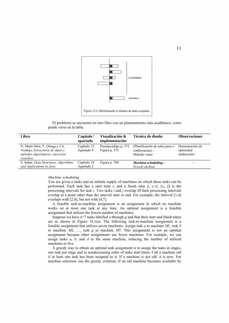
Problema 10 La Universidad Imponente tiene que planificar un evento cultural que consiste en n conferencias. Para cada conferencia se conoce la hora de comienzo y la de finalización fijada por los ponentes. Se ha pedido al Departamento de Informática que planifique las n conferencias distribuyéndolas entre las distintas salas disponibles, de forma que, claro está, no haya dos conferencias en una misma sala al mismo tiempo.

El objetivo es minimizar el número de salas utilizadas, para así causar el menor trastorno al resto de las actividades académicas.

11

El problema se encuentra en otro libro con un planteamiento más académico, como

puede verse en la tabla.






Pseudocódigo p. 373 Figura p. 373

(Planificación de salas para n conferencias) − Método voraz

Demostración de optimidad (inducción)

S. Sahni, Data Structures, Algorithms and Applications in Java


Figura p. 704 Machina scheduling − Greedy method

−

Machine scheduling You are given n tasks and an infinite supply of machines on which these tasks can be performed. Each task has a start time si and a finish time fi, si<fi. [si, fi] is the processing intervals for task i. Two tasks i and j overlap iff their processing intervals overlap at a point other than the interval start or end. For example, the interval [1,4] overlaps with [2,4], but not with [4,7].

A feasible task-to-machine assignment is an assignment in which no machine works on at most one task at any time. An optimal assignment is a feasible assignment that utilizes the fewest number of machines.

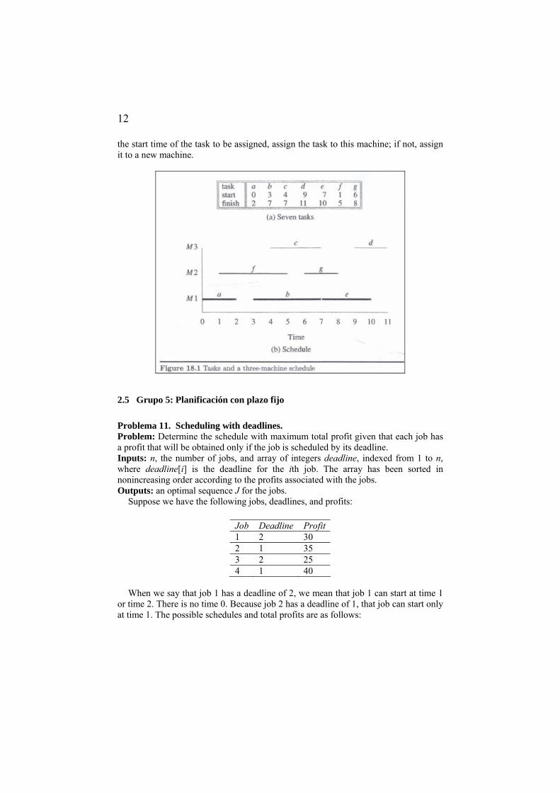
Suppose we have n=7 tasks labelled a through g and that their start and finish times are as shown in Figure 18.1(a). The following task-to-machine assignment is a feasible assignment that utilizes seven machines: Assign task a to machine M1, task b to machine M2, …, task g to machine M7. This assignment is not an optimal assignment because other assignments use fewer machines. For example, we can assign tasks a, b, and d to the same machine, reducing the number of utilized machines to five.

A greedy way to obtain an optimal task assignment is to assign the tasks in stages, one task per stage and in nondecreasing order of tasks start times. Call a machine old if at least one task has been assigned to it. If a machine is not old, it is new. For machine selection, use the greedy criterion: If an old machine becomes available by

12

the start time of the task to be assigned, assign the task to this machine; if not, assign it to a new machine.

2.5 Grupo 5: Planificación con plazo fijo

Problema 11. Scheduling with deadlines. Problem: Determine the schedule with maximum total profit given that each job has a profit that will be obtained only if the job is scheduled by its deadline. Inputs: n, the number of jobs, and array of integers deadline, indexed from 1 to n, where deadline[i] is the deadline for the ith job. The array has been sorted in nonincreasing order according to the profits associated with the jobs. Outputs: an optimal sequence J for the jobs.

Suppose we have the following jobs, deadlines, and profits:

Job Deadline Profit 1 2 30 2 1 35 3 2 25 4 1 40

When we say that job 1 has a deadline of 2, we mean that job 1 can start at time 1

or time 2. There is no time 0. Because job 2 has a deadline of 1, that job can start only at time 1. The possible schedules and total profits are as follows:

13

Schedule Total profit [1,3] 30+25 = 55 [2,1] 35+30 = 65 [2,3] 35+25 = 60 [3,1] 25+30 = 55 [4,1] 40+30 = 70 [4,3] 40+25 = 65

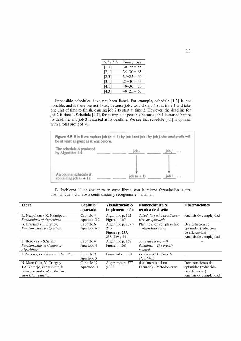
Impossible schedules have not been listed. For example, schedule [1,2] is not

possible, and is therefore not listed, because job i would start first at time 1 and take one unit of time to finish, causing job 2 to start at time 2. However, the deadline for job 2 is time 1. Schedule [1,3], for example, is possible because job 1 is started before its deadline, and job 3 is started at its deadline. We see that schedule [4,1] is optimal with a total profit of 70.

El Problema 11 se encuentra en otros libros, con la misma formulación u otra distinta, que incluimos a continuación y recogemos en la tabla.




Observaciones



Algoritmo p. 162 Figura p. 165

Scheduling with deadlines – Greedy approach




Algoritmo p. 237 y 240 Figuras p. 235, 238, 239 y 241

Planificación con plazo fijo – Algoritmo voraz

Demostración de optimidad (reducción de diferencias) Análisis de complejidad

E. Horowitz y S.Sahni, Fundamentals of Computer Algorithms



Job sequencing with deadlines – The greedy method

–


Enunciado p. 110 Problem 473 – Greedy algorithms

_



Algoritmos p. 377 y 378

(Las huertas del tío Facundo) – Método voraz

Demostraciones de optimidad (reducción de diferencias) Análisis de complejidad

14

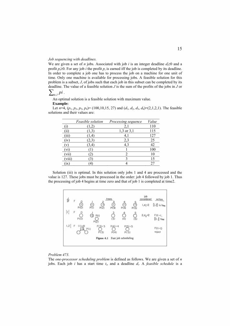
Planificación con plazo fijo. Tenemos que ejecutar un conjunto de n tareas, cada una de las cuales requiere un tiempo unitario. En cualquier instante t=1,2,… podemos ejecutar únicamente una tarea. La tarea i nos produce unos beneficios gi>0 sólo en el caso de que sea ejecutada en un instante anterior a di.

Por ejemplo, con n=4 y los valores siguientes:

i 1 2 3 4 gi 50 10 15 30 di 2 1 2 1

las planificaciones que hay que considerar y los beneficios correspondientes son:

Secuencia Beneficio 1 2 3 4

5 10 15 30

1,3 2,1 2,3 3,1 4,1 4,3

65 60 25 65 80 óptimo 45

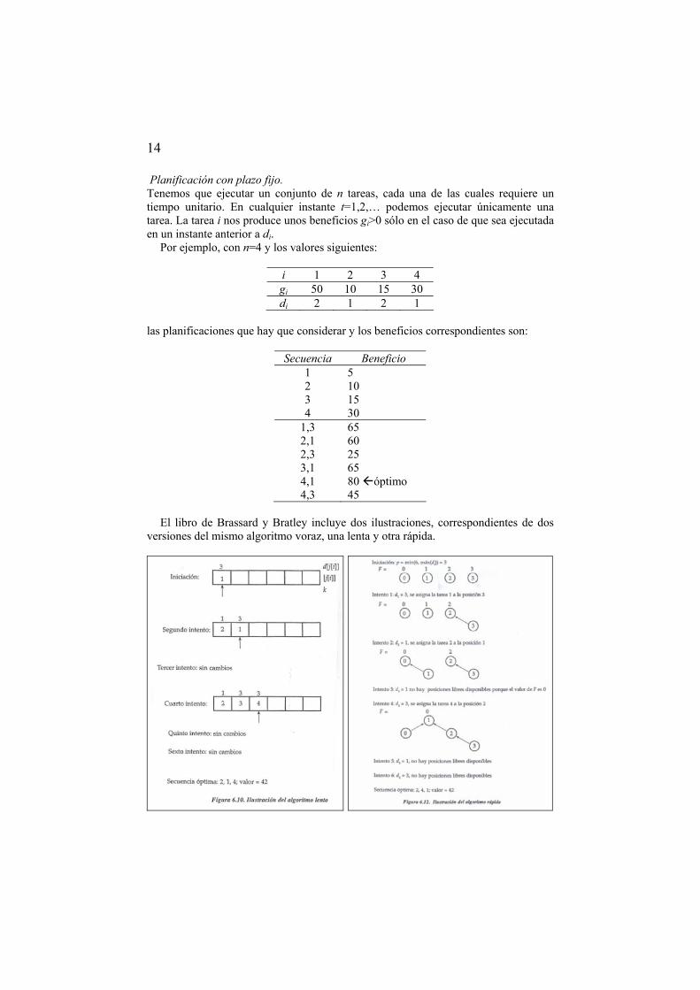
El libro de Brassard y Bratley incluye dos ilustraciones, correspondientes de dos

versiones del mismo algoritmo voraz, una lenta y otra rápida.

15

Job sequencing with deadlines. We are given a set of n jobs. Associated with job i is an integer deadline di≥0 and a profit pi≥0. For any job i the profit pi is earned iff the job is completed by its deadline. In order to complete a job one has to process the job on a machine for one unit of time. Only one machine is available for processing jobs. A feasible solution for this problem is a subset, J, of jobs such that each job in this subset can be completed by its deadline. The value of a feasible solution J is the sum of the profits of the jobs in J or

∑∈Jipi .

An optimal solution is a feasible solution with maximum value. Example: Let n=4, (p1, p2, p3, p4)= (100,10,15, 27) and (d1, d2, d3, d4)=(2,1,2,1). The feasible

solutions and their values are:

Feasible solution Processing sequence Value (i) (1,2) 2,1 110 (ii) (1,3) 1,3 or 3,1 115 (iii) (1,4) 4,1 127 (iv) (2,3) 2,3 25 (v) (3,4) 4,3 42 (vi) (1) 1 100 (vii) (2) 2 10 (viii) (3) 3 15 (ix) (4) 4 27

Solution (iii) is optimal. In this solution only jobs 1 and 4 are processed and the

value is 127. These jobs must be processed in the order: job 4 followed by job 1. Thus the processing of job 4 begins at time zero and that of job 1 is completed at time2.

Problem 473. The one-processor scheduling problem is defined as follows. We are given a set of n jobs. Each job i has a start time ti, and a deadline di. A feasible schedule is a

16

permutation of the jobs such that when the jobs are performed in that order, then every job is finished before the deadline. A greedy algorithm for the one-processor scheduling problem processes the jobs in order of deadline (the early deadlines before the late ones).

Show that if a feasible schedule exists, then the schedule produced by this greedy algorithm is feasible.

(Las huertas del tío Facundo) El tío Facundo posee n huertas, cada una con un tipo diferente de árboles frutales. Las frutas ya han madurado y es hora de recolectarlas. La recolección de una huerta exige un día completo. El tío Facundo conoce, para cada una de las huertas, el beneficio que obtendría por la venta de lo recolectado.

También sabe los días que tardan en pudrirse los frutos de cada huerta. − Problema 11. En estos casos, el manual de buen recolector sugiere utilizar una

estrategia voraz. Ayudar al tío Facundo a decidir qué debe recolectar y cuando debe hacerlo, para maximizar el beneficio total obtenido.

− Problema 12. Estudiar si la estrategia utilizada para solucionar el apartado anterior es válida también en el caso de que la recolección de cada huerta requiera un número arbitrario de días.

Libro Capítulo /





– (Las huertas del tío Facundo) – Método voraz

Contraejemplo

2.6 Grupo 6: Selección de actividades

Problema 13. An activity selection problem. Suppose we have a set S={a1,a2,…,an} of n proposed activities that wish to use a resource, such as a lecture hall, which can be used by only one activity at a time. Each activity ai has a start time si and a finish time fi, where 0≤si<fi<∞. If selected, activity ai takes place during the half-open time interval [si,fi). Activities ai and aj are compatible if the intervals [si,fi) and [sj,fj) do not overlap (i.e. ai and aj are compatible if si≥fj or sj≥fi). The activity-selection problem is to select a maximum-size subset of mutually compatible activities.

For example, consider the following set S of activities, which we have sorted in monotonically increasing order of finish time:

i 1 2 3 4 5 6 7 8 9 10 11 si 1 3 0 5 3 5 6 8 8 2 12 fi 4 5 6 7 8 9 10 11 12 13 14

17

El problema también lo encontramos en otro libro, como se aprecia en la tabla.




T. H. Cormen, C. E. Leiserson, R. L. Rivest y C. Stein, Introduction to algorithms


Pseudocódigo recursivo p. 376 Pseudocódigo iterativo p. 378 Figura p. 377

An activity-selection problem – Greedy algorithms

Demostración de optimidad p. 374 Análisis de complejidad




Método voraz Demostración de optimidad (reducción de diferencias)

18

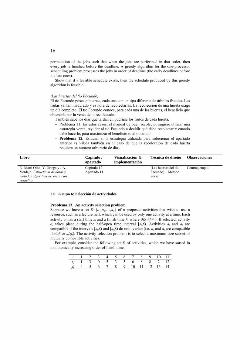
Maratón de cine. La filmoteca ha organizado un maratón de cine de terror. Durante 24 horas se proyectarán películas (todas diferentes) en las n salas disponibles. Deborah Cinema, gran aficionada a este género de películas, ha conseguido la programación completa donde aparecen todas las películas que se van a proyectar durante el maratón: junto con el título, nombre del director, duración de la película y otros datos de interés, se indica la sala de proyección y la hora de comienzo.

Ayudar a Deborah a planificar su maratón de cine, teniendo en cuenta que su único objetivo es ver el máximo número posible de películas.

2.7 Grupo 7

Problema 14 Una cinta magnética contiene n programas de longitudes l1, l2,…, ln. Se supone que tanto la densidad de información en la cinta como la velocidad de lectura son constantes, y que, tras cada búsqueda seguida de la lectura de un programa, la cinta es automáticamente rebobinada. Se conoce la tasa de utilización de cada programa; esto es, se sabe que del numero total de peticiones, un porcentaje pi corresponde al

programa i (1≤i≤n), con ∑ =

n

ipi

1= 1.

El objetivo es minimizar el tiempo medio de carga, el cual es proporcional a

∑ ∑= =

n

j

j

kikij lp

1 1

Cuando los programas están almacenados en el orden i1, i2,…,in. (a) Demostrar mediante un contraejemplo que la secuencia en orden creciente de li

no es necesariamente óptima. (b) Demostrar asimismo mediante un contraejemplo que la secuencia en orden de pi

decreciente no es necesariamente optima. (c) Demostrar por ultimo que la secuencia ordenada en forma decreciente de pi/li

minimiza el tiempo medio de carga.

19



Técnica de diseño

Observaciones



– Método voraz Contrajemplos p. 359 y 360 Demostración de optimidad (reducción de diferencias) p. 360

Scheduling to minimize average completion time. Suppose you are given a set S = {a1, a2, ..., an} of tasks, where task ai requires pi units of processing time to complete, once it has started. You have one computer on which to run these tasks, and the computer can run only one task at a time. Let ci be the completion time of task ai, that is, the time at which task ai completes processing. Your goal is to minimize the average completion time, that is, to minimize.

For example, suppose there are two tasks, a1 and a2, with p1 = 3 and p2 = 5, and consider the schedule in which a2 runs first, followed by a1. Then c2 = 5, c1 = 8, and the average completion time is (5 + 8) / 2 = 6.5. Problema 15. (a) Give an algorithm that schedules the tasks so as to minimize the average completion time. Each task must run non-preemptively, that is, once task ai is started, it must run continuously for pi units of time.

Prove that your algorithm minimizes the average completion time, and state the running time of your algorithm. Problema 16. (b) Suppose now that the tasks are not all available at once. That is, each task has a release time ri before which it is not available to be processed. Suppose also that we allow pre-emption, so that a task can be suspended and restarted at a later time. For example, a task ai with processing time pi = 6 may start running at time 1 and be pre-empted at time 4. It can then resume at time 10 but be pre-empted at time 11 and finally resume at time 13 and complete at time 15.

Task ai has run for a total of 6 time units, but its running time has been divided into three pieces. We say that the completion time of ai is 15.

Give an algorithm that schedules the tasks so as to minimize the average completion time in this new scenario. Prove that your algorithm minimizes the average completion time, and state the running time of your algorithm.


Capítulo 16 Apartado Problems

– Método voraz –

Problema de minimización de tareas en un sistema. Un sistema da servicio a n tareas, cada una con un tiempo de ejecución ti para i entre 1 y n. Se desea minimizar el tiempo medio de estancia de una tarea en el sistema, esto es, el tiempo transcurrido desde el comienzo de todo el proceso hasta que la tarea termina de ejecutarse.

Resolver el problema cuando: − Problema 15. Se dispone de un único procesador. − Problema 17. Se tienen s procesadores idénticos.

20

Ambos problemas se encuentran en otros libros, con la misma formulación u otras distintas. Comenzamos por el Problema 15.




Observaciones



– Método voraz –



– (Problema de minimización de tareas en un sistema) – Método voraz

Demostración de optimidad p. 355




Minimizing total time in the system – Greedy approach




Figura p. 233 Minimización del tiempo en el sistema – Algoritmo voraz


J. Gonzalo Arroyo y M. Rodríguez Artacho, Esquemas algorítmicos enfoque metodológico y problemas resueltos


Pseudocódigo p. 39

Problema de almacenamiento de programas en cinta – Algoritmos voraces




Algoritmo p. 156

Optimal storage on tapes – The greedy method

–


Enunciado p. 110 Problem 470 – Greedy algorithms

–

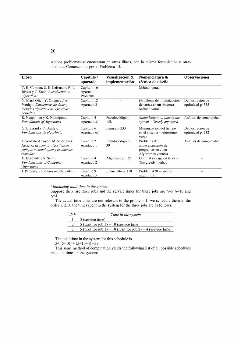
Minimizing total time in the system. Suppose there are three jobs and the service times for these jobs are t1=5 t2=10 and t3=4.

The actual time units are not relevant to the problem. If we schedule them in the order 1, 2, 3, the times spent in the system for the three jobs are as follows:

Job Time in the system 1 5 (service time) 2 5 (wait for job 1) + 10 (service time) 3 5 (wait for job 1) + 10 (wait for job 2) + 4 (service time)

The total time in the system for this schedule is 5+ (5+10) + (5+10+4) =39 This same method of computation yields the following list of all possible schedules

and total times in the system:

21

Schedule Total time in the system [1, 2, 3] 5+(5+10)+(5+10+4) = 39 [1, 3, 2] 5+(5+4)+(5+4+10) = 33 [2, 1, 3] 10+(10+5)+(10+5+4) = 44 [2, 3, 1] 10+(10+4)+(10+4+5) = 43 [3, 1, 2] 4+(4+5)+(4+5+10) = 32 [3, 2, 1] 4+(4+10)+(4+10+5) = 37

Schedule [3, 1, 2] is optimal with a total time of 32.

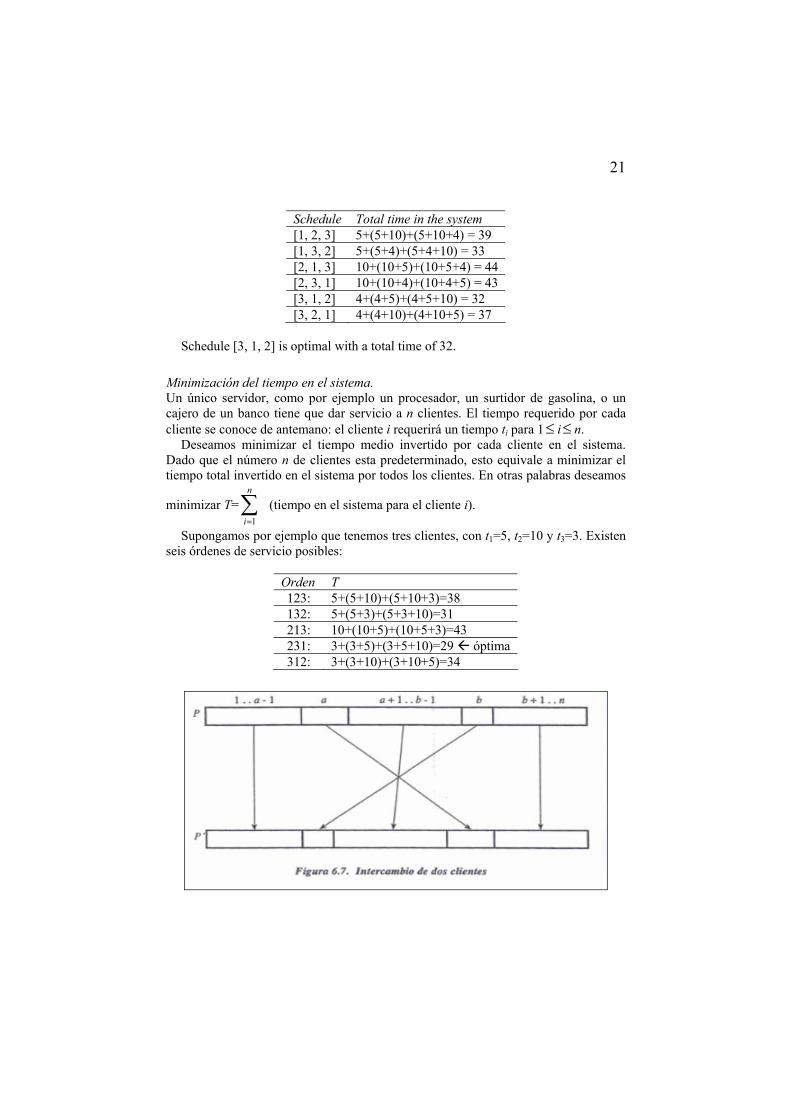
Minimización del tiempo en el sistema. Un único servidor, como por ejemplo un procesador, un surtidor de gasolina, o un cajero de un banco tiene que dar servicio a n clientes. El tiempo requerido por cada cliente se conoce de antemano: el cliente i requerirá un tiempo ti para 1≤ i≤ n.

Deseamos minimizar el tiempo medio invertido por cada cliente en el sistema. Dado que el número n de clientes esta predeterminado, esto equivale a minimizar el tiempo total invertido en el sistema por todos los clientes. En otras palabras deseamos

minimizar T=∑=

n

i 1

(tiempo en el sistema para el cliente i).

Supongamos por ejemplo que tenemos tres clientes, con t1=5, t2=10 y t3=3. Existen seis órdenes de servicio posibles:

Orden T 123: 5+(5+10)+(5+10+3)=38 132: 5+(5+3)+(5+3+10)=31 213: 10+(10+5)+(10+5+3)=43 231: 3+(3+5)+(3+5+10)=29 óptima 312: 3+(3+10)+(3+10+5)=34

22

Problema de almacenamiento de programas en cinta. Consideramos un conjunto de programas p1, p2,.., pn que ocupan un espacio en una cinta l1, l2,…,ln.

Diseñar un algoritmo para almacenarlos en una cinta de modo que el tiempo medio de acceso sea mínimo.

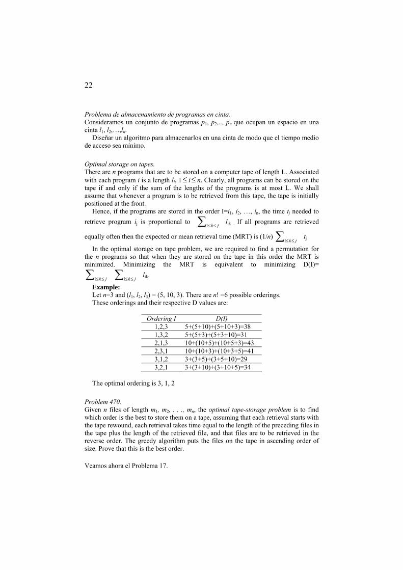
Optimal storage on tapes. There are n programs that are to be stored on a computer tape of length L. Associated with each program i is a length li, 1≤ i≤ n. Clearly, all programs can be stored on the tape if and only if the sum of the lengths of the programs is at most L. We shall assume that whenever a program is to be retrieved from this tape, the tape is initially positioned at the front.

Hence, if the programs are stored in the order I=i1, i2, …, in, the time tj needed to retrieve program ij is proportional to ∑ ≤≤ jk1

lik . If all programs are retrieved

equally often then the expected or mean retrieval time (MRT) is (1/n) ∑ ≤≤ jk1tj

In the optimal storage on tape problem, we are required to find a permutation for the n programs so that when they are stored on the tape in this order the MRT is minimized. Minimizing the MRT is equivalent to minimizing D(I)=

∑ ≤≤ jk1 ∑ ≤≤ jk1lik.

Example: Let n=3 and (l1, l2, l3) = (5, 10, 3). There are n! =6 possible orderings. These orderings and their respective D values are:

Ordering I D(I) 1,2,3 5+(5+10)+(5+10+3)=38 1,3,2 5+(5+3)+(5+3+10)=31 2,1,3 10+(10+5)+(10+5+3)=43 2,3,1 10+(10+3)+(10+3+5)=41 3,1,2 3+(3+5)+(3+5+10)=29 3,2,1 3+(3+10)+(3+10+5)=34

The optimal ordering is 3, 1, 2

Problem 470. Given n files of length m1, m2, . . ., mn, the optimal tape-storage problem is to find which order is the best to store them on a tape, assuming that each retrieval starts with the tape rewound, each retrieval takes time equal to the length of the preceding files in the tape plus the length of the retrieved file, and that files are to be retrieved in the reverse order. The greedy algorithm puts the files on the tape in ascending order of size. Prove that this is the best order. Veamos ahora el Problema 17.

23

Libro Capítulo /



Observaciones



– (Problema de minimización de tareas en un sistema) – Método voraz




Figura p. 234 Flow shop scheduling – Dynamic programming

–

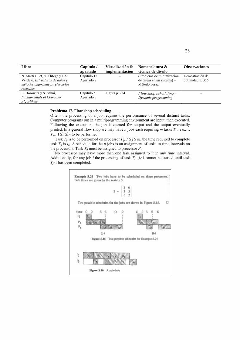
Problema 17. Flow shop scheduling Often, the processing of a job requires the performance of several distinct tasks. Computer programs run in a multiprogramming environment are input, then executed. Following the execution, the job is queued for output and the output eventually printed. In a general flow shop we may have n jobs each requiring m tasks T1i, T2i,…, Tmi, 1≤ i≤ n to be performed.

Task Tji is to be performed on processor Pj, 1≤ j≤m, the time required to complete task Tji is tji. A schedule for the n jobs is an assignment of tasks to time intervals on the processors. Task Tji must be assigned to processor Pj.

No processor may have more than one task assigned to it in any time interval. Additionally, for any job i the processing of task Tji, j>1 cannot be started until task Tj-1 has been completed.

24

2.8 Agrupamiento de problemas

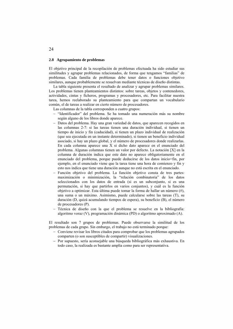
El objetivo principal de la recopilación de problemas efectuada ha sido estudiar sus similitudes y agrupar problemas relacionados, de forma que tengamos “familias” de problemas. Cada familia de problemas debe tener datos o funciones objetivo similares, aunque probablemente se resuelvan mediante técnicas de diseño distintas.

La tabla siguiente presenta el resultado de analizar y agrupar problemas similares. Los problemas tienen planteamientos distintos: sobre tareas, objetos y contenedores, actividades, cintas y ficheros, programas y procesadores, etc. Para facilitar nuestra tarea, hemos reelaborado su planteamiento para que compartan un vocabulario común, el de tareas a realizar en cierto número de procesadores.

Las columnas de la tabla corresponden a cuatro grupos: − “Identificador” del problema. Se ha tomado una numeración más su nombre

según alguno de los libros donde aparece. − Datos del problema. Hay una gran variedad de datos, que aparecen recogidos en

las columnas 2-7: si las tareas tienen una duración individual, si tienen un tiempo de inicio y fin (caducidad), si tienen un plazo individual de realización (que sea ejecutada en un instante determinado), si tienen un beneficio individual asociado, si hay un plazo global, y el número de procesadores donde realizarlas. En cada columna aparece una X si dicho dato aparece en el enunciado del problema. Algunas columnas tienen un valor por defecto. La notación [X] en la columna de duración indica que este dato no aparece obligatoriamente en el enunciado del problema, porque puede deducirse de los datos inicio+fin, por ejemplo, en el enunciado viene que la tarea tiene una hora de comienzo y fin y esto nos indica que tiene una duración aunque no está escrita en el enunciado.

− Función objetivo del problema. La función objetivo consta de tres partes: maximización o minimización, la “relación combinatoria” de los datos seleccionados con los datos de entrada (si es un subconjunto, si es una permutación, si hay que partirlos en varios conjuntos), y cuál es la función objetivo a optimizar. Esta última puede tomar la forma de hallar un número (#), una suma o un máximo. Asimismo, puede calcularse sobre las tareas (T), su duración (D, quizá acumulando tiempos de espera), su beneficio (B), el número de procesadores (P).

− Técnica de diseño con la que el problema se resuelve en la bibliografía: algoritmo voraz (V), programación dinámica (PD) o algoritmo aproximado (A).

El resultado son 7 grupos de problemas. Puede observarse la similitud de los problemas de cada grupo. Sin embargo, el trabajo no está terminado porque:

− Conviene revisar los libros citados para comprobar que los problemas agrupados comparten (o son susceptibles de compartir) visualizaciones.

− Por supuesto, sería aconsejable una búsqueda bibliográfica más exhaustiva. En todo caso, la realizada es bastante amplia como para ser representativa.

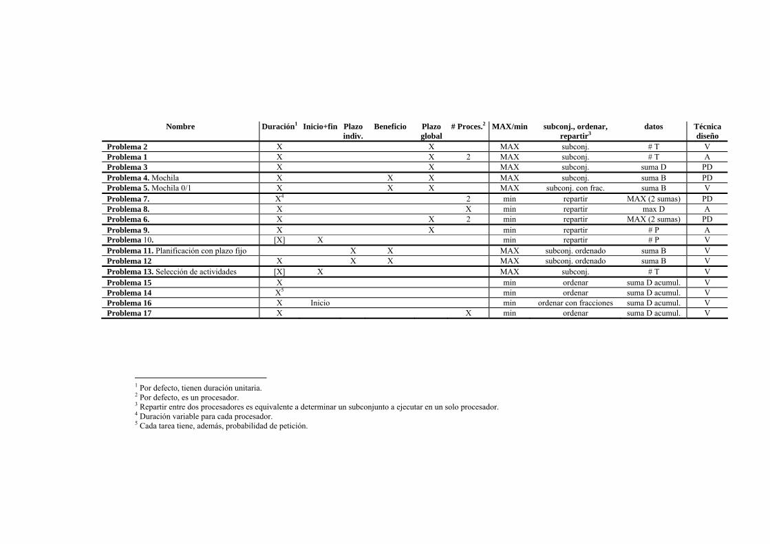
Nombre Duración1 Inicio+fin Plazo

indiv.Beneficio Plazo

global # Proces.2 MAX/min subconj., ordenar,

repartir3 datos Técnica

diseño Problema 2 X X MAX subconj. # T V Problema 1 X X 2 MAX subconj. # T A Problema 3 X X MAX subconj. suma D PD Problema 4. Mochila X X X MAX subconj. suma B PD Problema 5. Mochila 0/1 X X X MAX subconj. con frac. suma B V Problema 7. X4 2 min repartir MAX (2 sumas) PD Problema 8. X X min repartir max D A Problema 6. X X 2 min repartir MAX (2 sumas) PD Problema 9. X X min repartir # P A Problema 10. [X] X min repartir # P V Problema 11. Planificación con plazo fijo X X MAX subconj. ordenado suma B V Problema 12 X X X MAX subconj. ordenado suma B V Problema 13. Selección de actividades [X] X MAX subconj. # T V Problema 15 X min ordenar suma D acumul. V Problema 14 X5 min ordenar suma D acumul. V Problema 16 X Inicio min ordenar con fracciones suma D acumul. V Problema 17 X X min ordenar suma D acumul. V

1 Por defecto, tienen duración unitaria. 2 Por defecto, es un procesador. 3 Repartir entre dos procesadores es equivalente a determinar un subconjunto a ejecutar en un solo procesador. 4 Duración variable para cada procesador. 5 Cada tarea tiene, además, probabilidad de petición.

3 Problemas de monedas

3.1 Problema del cambio de monedas

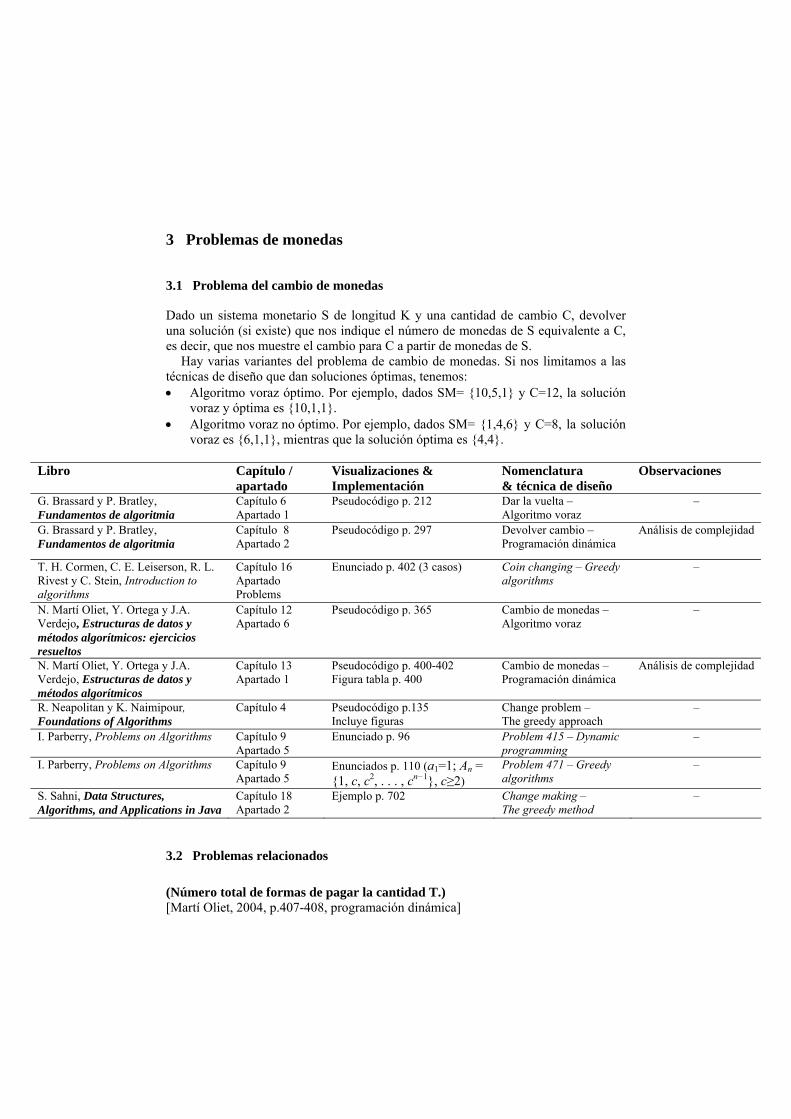
Dado un sistema monetario S de longitud K y una cantidad de cambio C, devolver una solución (si existe) que nos indique el número de monedas de S equivalente a C, es decir, que nos muestre el cambio para C a partir de monedas de S.

Hay varias variantes del problema de cambio de monedas. Si nos limitamos a las técnicas de diseño que dan soluciones óptimas, tenemos: • Algoritmo voraz óptimo. Por ejemplo, dados SM= {10,5,1} y C=12, la solución

voraz y óptima es {10,1,1}. • Algoritmo voraz no óptimo. Por ejemplo, dados SM= {1,4,6} y C=8, la solución

voraz es {6,1,1}, mientras que la solución óptima es {4,4}.


Visualizaciones & Implementación


Observaciones



Pseudocódigo p. 212 Dar la vuelta – Algoritmo voraz

–



Pseudocódigo p. 297 Devolver cambio – Programación dinámica




Enunciado p. 402 (3 casos) Coin changing – Greedy algorithms

–




Cambio de monedas – Algoritmo voraz

–

N. Martí Oliet, Y. Ortega y J.A. Verdejo, Estructuras de datos y métodos algorítmicos


Pseudocódigo p. 400-402 Figura tabla p. 400

Cambio de monedas – Programación dinámica



Capítulo 4 Pseudocódigo p.135 Incluye figuras

Change problem – The greedy approach

–


Enunciado p. 96 Problem 415 – Dynamic programming

–


Enunciados p. 110 (a1=1; An = {1, c, c2, . . . , cn−1}, c≥2)

Problem 471 – Greedy algorithms

–



Ejemplo p. 702 Change making – The greedy method

–

3.2 Problemas relacionados

(Número total de formas de pagar la cantidad T.) [Martí Oliet, 2004, p.407-408, programación dinámica]

27

El país de Fanfanisflán emite n sellos diferentes de valores naturales positivos s1, s2, ..., sn. Se quiere enviar una carta y se sabe que la correspondiente tarifa postal es T. ¿De cuántas formas diferentes se puede franquear exactamente la carta, si el orden de los sellos no importa?

La cantidad máxima de dinero que se puede obtener haciendo inversiones adecuadas [Martí Oliet, 2004, p.430-431, programación dinámica, incluye figura temporal] Mr. Scrooge dispone de una cierta cantidad de dinero M que quiere invertir durante n meses. Al principio de cada mes puede elegir una de entre las tres opciones siguientes, destinando a ella todo su dinero disponible en ese momento: 1. Comprar certificados de deposito de un mes del Banco Usureros & Co., cuya

comisión fija (no depende de la cantidad invertida) en el tiempo t de compra es GCD (t), es decir, una cantidad de dinero x invertida en el tiempo t se convierte en la cantidad (x-GCD(t))*RCD(t) en el tiempo t+1.

2. Comprar bonos del tesoro de Corruplandia de seis meses. Los gastos de compra en el tiempo t son GBT(t) (también fijos) y el correspondiente rendimiento a los seis meses es RBT(t).

3. Guardar el dinero en un calcetín y ponerlo debajo del colchón (durante un mes). Suponiendo que Mr.Scrooge tiene predicciones fiables de GCD; RCD, GBT y

RBT para los n meses siguientes, desarrollar un algoritmo eficiente para calcular la cantidad máxima de dinero que puede obtener haciendo las inversiones adecuadas.

Problem 416 [Parberry, 1995, p.97, dynamic programming] Arbitrage is the use of discrepancies in currency-exchange rates to make a profit. For example, there may be a small window of time during which 1 U.S. dollar buys 0.75 British pounds, 1 British pound buys 2 Australian dollars, and 1 Australian dollar buys 0.70 U.S. dollars. Then, a smart trader can trade one U.S. dollar and end up with 0.75 × 2 × 0.7 = 1.05 U.S. dollars, a profit of 5%.

Suppose that there are n currencies c1, . . ., cn, and an n × n table R of exchange rates, such that one unit of currency ci buys R[i, j] units of currency cj .

Devise and analyze a dynamic programming algorithm to determine the maximum value of R [c1, ci1] · R[ci1, ci2 ] · · ·R[cik-1, cik] · R[cik, c1].

Problem 417 [Parberry, 1995, p.97, dynamic programming] You have $1 and want to invest it for n months. At the beginning of each month, you must choose from the following three options: (a) Purchase a savings certificate from the local bank. Your money will be tied up

for one month. If you buy it at time t, there will be a fee of CS(t) and after a month, it will return S(t) for every dollar invested. That is, if you have $k at time t, then you will have $(k − CS (t))S(t) at time t + 1.

(b) Purchase a state treasury bond. Your money will be tied up for six months. If you buy it at time t, there will be a fee of CB (t) and after six months, it will return

28

B(t) for every dollar invested. That is, if you have $k at time t, then you will have $(k − CB (t))B(t) at time t + 6.

(c) Store the money in a sock under your mattress for a month. That is, if you have $k at time t, then you will have $k at time t + 1.

Suppose you have predicted values for S, B, CS, and CB for the next n months. Devise a dynamic programming algorithm that computes the maximum amount of

money that you can make over the n months in time O(n).

29

4 Problemas de mezcla de cintas

Se trata de un problema bastante frecuente y conocido.




Observaciones

J. Gonzalo Arroyo y M. Rodríguez Artacho, Esquemas algorítmicos enfoque metodológico y problemas resueltos


Algoritmo p. 42 Algoritmos voraces Análisis de complejidad

E.Horowitz y S.Sahni, Fundamentals of Computer Algorithms


Algoritmo p. 171

Optimal merge patterns – The greedy method

–




12.12 – Método voraz Demostración de optimidad (inducción)

Dado un conjunto de n cintas no vacías con ni registros ordenados cada una, se pretende mezclarlas a pares hasta lograr una única cinta ordenada. La secuencia en la que se realiza la mezcla determinara la eficiencia de proceso. Diséñese un algoritmo que busque la solución óptima minimizando el número de movimientos.

Por ejemplo: 3 cintas: A con 30 registros, B con 20 y C con 10. Mezclamos A con B (50 movimientos) y luego el resultado con C (60), con lo que realizamos en total 110 movimientos.

Optimal merge patterns Two sorted files containing n and m records respectively could be merged together to obtain one sorted file in time O (n + m). When more than two sorted files are to be merged together the merge can be accomplished by repeatedly merging sorted files in pairs. Thus, if files X1, X2, X3 and X4 are to be merged we could first merge X1 and X2 to get a file Y1. Then we could merge Y1 and X3 to get Y2. Finally, Y2 and X4 could be merged to obtain the desired sorted file.

Alternatively, we could first merge X1 and X2 getting Y1, then merge X3 and X4 getting Y2 and finally Y1 and Y2 getting the desired sorted file. Given n sorted files there are many ways in which to pair wise merge them into a single sorted file. Different pairings require differing amounts of computing time. The problem we shall address ourselves to now is that of determining an optimal (i.e. one requiring the fewest comparisons) way to pair wise merge n sorted files together. Example: X1, X2 and X3 are three sorted files of length 30, 20 and 10 records each. Merging X1 and X2 requires 50 record moves. Merging the result with X3 requires another 60 moves. The total number of record moves required to merge the three files this way is 110. If instead, we first merge X2 and X3 (taking 30 moves) and then X1 (taking 60 moves); the total record moves made is only 90. Hence, the second mere pattern is faster than the first.

30

Minimización del trabajo de la mezcla de fichas El Maestro Piero, profesor de musicología del Real Conservatorio de Cantalarrana, guarda las fichas de todos los alumnos que ha tenido a lo largo de los últimos n años en su curso de Nanas en la Edad de Piedra. Para cada año, el lote de fichas está ordenado alfabéticamente. Pero ahora su afán es reunir todos los lotes en uno solo, igualmente ordenado (se supone que todos los lotes son disjuntos, ya que los alumnos se matriculan una sola vez con él porque todos aprueban).

Para obtener el lote conjunto, el Maestro ha de ir mezclando (de forma ordenada) pares de lotes de fichas. Pero, puesto que el tiempo empleado en la mezcla ordenada depende de los tamaños de los lotes a mezclar, no da lo mismo mezclar unos antes que otros. Encontrar una estrategia que determine el orden en el que se han de mezclar los lotes para minimizar el trabajo total de mezcla.

31

5 Problemas de cadenas de caracteres

5.1 La subsecuencia común más larga

En el problema de la subsecuencia común más larga (SCML) se consideran dos secuencias: X =<x1,…, xm> e Y =<y1,…, yn>.

Se dice que Z =<z1,…, zk> es una subsecuencia de X si existe una secuencia de índices de X, i1,…, ik tal que xi j = zj para j = 1, 2,…, k. Z será común a X e Y si es subsecuencia de ambas y será una SCML si no existe otra de longitud mayor.




Observaciones

M. H. Alsuwaiyel, Algorithms Design Techniques and Analysis


Pseudocódigo p. 207 The longest common subsequence problem – Dynamic programming


S. Baase y A. Van Gelder, Computer Algorithms: Introduction to Design and Analysis


Pseudocódigo p. 474 Separating sequences of words into lines – Dynamic programming


T. H. Cormen, C. E. Leiserson, R. L. Rivest y C. Stein, Introduction to Algorithms



Longest common subsequence – Dynamic programming


M. T. Goodrich y R. Tamassia, Data Structures and Algorithms in Java


Algoritmo p. 505 The longest common subsequence problem – Dynamic programming




Ejemplo p. 263 Figuras

El problema de la subsecuencia común más larga – Programación dinámica


S. Skeina, the algorithm design manual

Capítulo3 Apartado 1.4

Ejemplo p. 62 Longest increasing sequence – Dynamic programming


5.2 Otros problemas de cadenas de caracteres

Separating sequences of words into lines [Baase, 2000, p.471-474, dynamic programming, incluye el algoritmo] The problem is separating a sequence of words into a series of lines that comprise a paragraph. The objective is to avoid a lot of extra spaces on any line. This is an important problem in computerized typesetting. Because extra spaces on the last line of the paragraph are not objectionable, the paragraph is a natural unit to optimize. Of course, the order of the words must be maintained as they are placed in lines.

The input to the line-breaking problem is a sequence of n word lengths, w1,…, wn, representing the lengths of words that make up a paragraph, and a line width W.

32

The basic constraint on word placement is that, if words i through j are placed on a single line, then wi+…+wj≤ W. in this case the number of extra spaces is

X=W-(wi+…+wj) The penalty for extra spaces is assumed to be some function of X. For our

discussion, the line penalty is specified as X3. Example: We take to be the whole paragraph

i 1 2 3 4 5 6 7 8 9 10 11 Those who cannot remember the past are condemned to repeat it Wi 6 4 7 9 4 5 4 10 3 7 4

Suppose w=17. The greedy strategy groups words into lines as follows:

Words (1,2,3) (4,5) (6,7) (8,9) (10,11) X 0 4 8 4 0 Penalti 0 64 512 64 0

Problema de convertir una cadena de caracteres a otra [Martí Oliet, 2004, p.432-435, programación dinámica, incluye figura de tabla] Sean A=a1a2...an y B=b1b2...bm dos cadenas sobre un alfabeto finito de caracteres desea transformar A en B utilizando una serie de cambios de caracteres de las tres siguientes clases:

Insertar(c, k) Insertar el carácter c en la posición k de la cadena Borrar (k) Borra el carácter en la posición k de la cadena Sustituir(c,k) Sustituye el carácter en la posición k de la cadena por el carácter c

Por ejemplo, la cadena abbc se transforma en la cadena babb y sustituir los tres

siguientes cambios: borrar la a (quedando bbc), insertar una a entre las b (babc) y sustituir la c por una b.

También se puede conseguir mediante sólo dos cambios: insertar b al principio (babbc) y borrar la c.

Desarrollar un algoritmo para saber cuál es el número mínimo de cambios necesarios para transformar A en B y cuáles son tales cambios.

Approximate string matching [Skeina, 1998, p.60-62, dynamic programming, incluye tabla] An important task in text processing is string matching, finding all the occurrences of a word in the text. Unfortunately, many words in documents are mispelled (sic). How can we search for the string closest to a given pattern in order to account for spelling errors?

To be more precise, let P be a pattern string and T a text string over the same alphabet. The edit distance between P and T is the smallest number of changes sufficient to transform a substring of T into P, where the changes may be: 1. Substitution - two corresponding characters may differ: KAT CAT.

33

2. Insertion - we may add a character to T that is in P: CT CAT. 3. Deletion - we may delete from T a character that is not in P: CAAT CAT.

For example, P=abcdefghijkl can be matched to T=bcdeffghixkl using exactly three changes, one of each of the above types.

Problem 407 [Parberry, p. 92, dynamic programming] A context-free grammar in Chomsky Normal Form consists of: • A set of nonterminal symbols N. • A set of terminal symbols T. • A special nonterminal symbol called the root. • A set of productions of the form either A → BC, or A → a, where A, B, C ∈ N, a

∈ T. If A ∈ N, define L(A) as follows:

L(A) = {bc | b ∈ L(B), c∈ L(C), where A → BC} ∪ {a | A → a} The language generated by a grammar with root R is defined to be L(R). The

CFL recognition problem is the following: For a fixed context-free grammar in Chomsky Normal Form, on input a string of

terminals x, determine whether x is in the language generated by the grammar. Devise an algorithm for the CFL recognition problem. Analyze your algorithm.

Problem 408 [Parberry, 1995, p. 92, dynamic programming] Fill in the tables in the dynamic programming algorithm for the CFL recognition problem (see Problem 407) on the following inputs. In each case, the root symbol is S. (a) Grammar: S → SS, S → s. String: ssssss. (b) Grammar: S → AR, S → AB, A → a, R → SB, B → b. String: aaabbb. (c) Grammar: S → AX, X → SA, A → a, S → BY , Y → SB, B → b, S → CZ, Z →

SC, C → c. String: abacbbcaba.

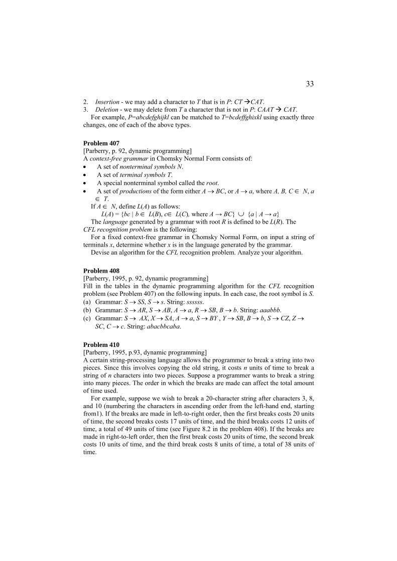
Problem 410 [Parberry, 1995, p.93, dynamic programming] A certain string-processing language allows the programmer to break a string into two pieces. Since this involves copying the old string, it costs n units of time to break a string of n characters into two pieces. Suppose a programmer wants to break a string into many pieces. The order in which the breaks are made can affect the total amount of time used.

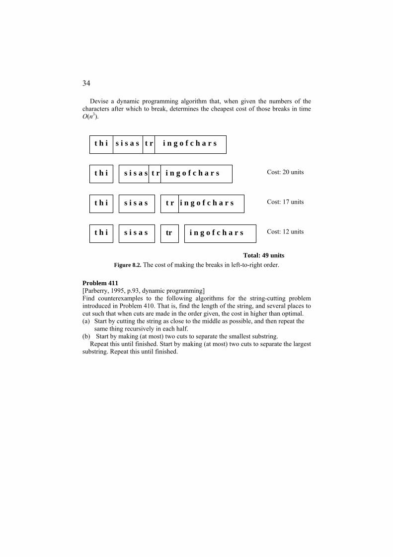
For example, suppose we wish to break a 20-character string after characters 3, 8, and 10 (numbering the characters in ascending order from the left-hand end, starting from1). If the breaks are made in left-to-right order, then the first breaks costs 20 units of time, the second breaks costs 17 units of time, and the third breaks costs 12 units of time, a total of 49 units of time (see Figure 8.2 in the problem 408). If the breaks are made in right-to-left order, then the first break costs 20 units of time, the second break costs 10 units of time, and the third break costs 8 units of time, a total of 38 units of time.

34

Devise a dynamic programming algorithm that, when given the numbers of the characters after which to break, determines the cheapest cost of those breaks in time O(n3).

Figure 8.2. The cost of making the breaks in left-to-right order.

Problem 411 [Parberry, 1995, p.93, dynamic programming] Find counterexamples to the following algorithms for the string-cutting problem introduced in Problem 410. That is, find the length of the string, and several places to cut such that when cuts are made in the order given, the cost in higher than optimal. (a) Start by cutting the string as close to the middle as possible, and then repeat the

same thing recursively in each half. (b) Start by making (at most) two cuts to separate the smallest substring.

Repeat this until finished. Start by making (at most) two cuts to separate the largest substring. Repeat this until finished.

t h i s i s a s t r i n g o f c h a r s

t r i n g o f c h a r s

t h i

s i s a s t r i n g o f c h a r s t h i

s i s a s t h i

s i s a s tr i n g o f c h a r s

Cost: 20 units

Cost: 17 units

Cost: 12 units

Total: 49 units

35

Figure 8.3. The cost of making the breaks in right-to-left order.

Problem 412 [Parberry, 1995, p.94, dynamic programming] There are two warehouses V and W from which widgets are to be shipped to destinations Di, 1≤i≤n. Let di be the demand at Di, for 1≤i≤n, and rV, rW be the number of widgets available at V and W, respectively.

Assume that there are enough widgets available to fill the demand, that is, that

rv+rw=∑=

n

iid

1

Let vi be the cost of shipping a widget from warehouse V to destination Di, and wi be the cost of shipping a widget from warehouse W to destination Di, for 1≤i≤n. The warehouse problem is the problem of finding xi, yi∈N for 1≤i≤n such that when xi widgets are sent from V to Di and yi widgets are sent from W to Di:

The demand at Di is filled, that is, xi + yi = di,

The inventory at V is sufficient, that is, rvxn

i i =∑ =1

The inventory at W is sufficient, that is, rwyn

i i =∑ =1

And the total cost of shipping the widgets,

iii

n

ii ywxv +∑

=1 is minimized.

Let gj(x) be the cost incurred when V has an inventory of x widgets, and supplies are sent to destinations Di for all 1≤i≤j in the optimal manner (note that W is not mentioned because knowledge of the inventory for V implies knowledge of the inventory for W, by (8.1).) Write a recurrence relation for gj(x) in terms of gj−1.

t h i s i a s t r i n g o f c h a r s

i n g o f c h a r s

t h i

i n g o f c h a r s t h i s i s as t r

s i s a s t h i

s i s a s tr i n g o f c h a r s

Cost: 20 units

Cost: 10 units

Cost: 8 units

Total: 38 units

tr

36

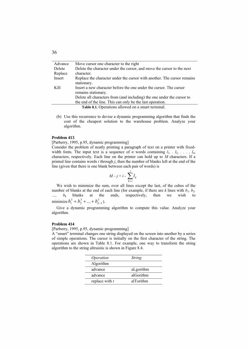
Advance Delete Replace Insert Kill

Move cursor one character to the right Delete the character under the cursor, and move the cursor to the next character. Replace the character under the cursor with another. The cursor remains stationary. Insert a new character before the one under the cursor. The cursor remains stationary. Delete all characters from (and including) the one under the cursor to the end of the line. This can only be the last operation.

Table 8.1. Operations allowed on a smart terminal.

(b) Use this recurrence to devise a dynamic programming algorithm that finds the cost of the cheapest solution to the warehouse problem. Analyze your algorithm.

Problem 413 [Parberry, 1995, p.95, dynamic programming] Consider the problem of neatly printing a paragraph of text on a printer with fixed-width fonts. The input text is a sequence of n words containing l1, . l2, . . . , ln, characters, respectively. Each line on the printer can hold up to M characters. If a printed line contains words i through j, then the number of blanks left at the end of the line (given that there is one blank between each pair of words) is

M – j + i - ∑=

j

ikkl

We wish to minimize the sum, over all lines except the last, of the cubes of the number of blanks at the end of each line (for example, if there are k lines with b1, b2, …, bk blanks at the ends, respectively, then we wish to minimize 3

132

31 ... −+++ kbbb ).

Give a dynamic programming algorithm to compute this value. Analyze your algorithm.

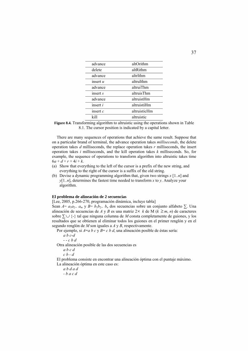
Problem 414 [Parberry, 1995, p.95, dynamic programming] A “smart” terminal changes one string displayed on the screen into another by a series of simple operations. The cursor is initially on the first character of the string. The operations are shown in Table 8.1. For example, one way to transform the string algorithm to the string altruistic is shown in Figure 8.4.

Operation String Algorithm advance aLgorithm advance alGorithm replace with t alTorithm

37

advance altOrithm delete altRithm advance altrIthm insert u altruIthm advance altruiThm insert s altruisThm advance altruistHm insert i altruistiHm insert c altruisticHm kill altruistic

Figure 8.4. Transforming algorithm to altruistic using the operations shown in Table 8.1. The cursor position is indicated by a capital letter.

There are many sequences of operations that achieve the same result. Suppose that

on a particular brand of terminal, the advance operation takes milliseconds, the delete operation takes d milliseconds, the replace operation takes r milliseconds, the insert operation takes i milliseconds, and the kill operation takes k milliseconds. So, for example, the sequence of operations to transform algorithm into altruistic takes time 6a + d + r + 4i + k. (a) Show that everything to the left of the cursor is a prefix of the new string, and

everything to the right of the cursor is a suffix of the old string. (b) Devise a dynamic programming algorithm that, given two strings x [1..n] and

y[1..n], determines the fastest time needed to transform x to y. Analyze your algorithm.

El problema de alineación de 2 secuencias [Lee, 2005, p.266-270, programación dinámica, incluye tabla] Sean A= a1a2.. am y B= b1b2.. bn dos secuencias sobre un conjunto alfabeto ∑. Una alineación de secuencias de A y B es una matriz 2× k de M (k ≥m, n) de caracteres sobre ∑∪ {-} tal que ninguna columna de M consta completamente de guiones, y los resultados que se obtienen al eliminar todos los guiones en el primer renglón y en el segundo renglón de M son iguales a A y B, respectivamente.

Por ejemplo, si A=a b c y B= c b d, una alineación posible de éstas sería: a b c-d - - c b d

Otra alineación posible de las dos secuencias es a b c d c b - d

El problema consiste en encontrar una alineación óptima con el puntaje máximo. La alineación óptima en este caso es:

a b d a d - b a c d

38

6 Problemas de multiplicación de matrices

6.1 Multiplicación encadenada de matrices

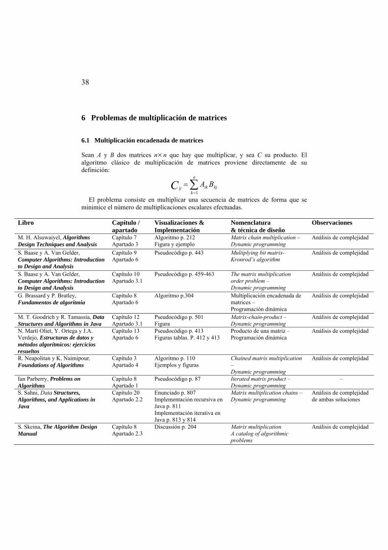
Sean A y B dos matrices n×n que hay que multiplicar, y sea C su producto. El algoritmo clásico de multiplicación de matrices proviene directamente de su definición:

kj

n

kikij BAC ∑

=

=1

El problema consiste en multiplicar una secuencia de matrices de forma que se minimice el número de multiplicaciones escalares efectuadas.

Libro Capítulo /

apartado Visualizaciones & Implementación


Observaciones



Algoritmo p. 212 Figura y ejemplo

Matrix chain multiplication – Dynamic programming




Pseudocódigo p. 443 Multiplying bit matrix-Kronrod’s algorithm




Pseudocódigo p. 459-463 The matrix multiplication order problem – Dynamic programming




Algoritmo p.304 Multiplicación encadenada de matrices – Programación dinámica




Pseudocódigo p. 501 Figura

Matrix-chain-product – Dynamic programming




Pseudocódigo p. 413 Figuras tablas. P. 412 y 413

Producto de una matriz – Programación dinámica




Algoritmo p. 110 Ejemplos y figuras

Chained matrix multiplication – Dynamic programming


Ian Parberry, Problems on Algorithms


Pseudocódigo p. 87 Iterated matrix product – Dynamic programming

–



Enunciado p. 807 Implementación recursiva en Java p. 811 Implementación iterativa en Java p. 813 y 814

Matrix multiplication chains – Dynamic programming

Análisis de complejidad de ambas soluciones

S. Skeina, The Algorithm Design Manual


Discussión p. 204 Matrix multiplication A catalog of algorithmic problems


39


Minimum Multiplications [Neapolitan, 1997, p.110-112, dynamic programming] Problem: Determining the minimum number of elementary multiplications needed to multiply n matrices and an order that produces that minimum number. Inputs: The number of matrices n, and an array of integers d, indexed from 0 to n, where d [i − 1] x d [i] is the dimension of the ith matrix.

Print Optimal Order [Neapolitan, 1997, p.112-113, dynamic programming] Problem: Print the optimal order for multiplying n matrices. Inputs: Positive integer n, and the array P. P[i][j] is the point where matrices i through j are split in an optimal order for multiplying those matrices. Outputs: The optimal order for multiplying the matrices.

40

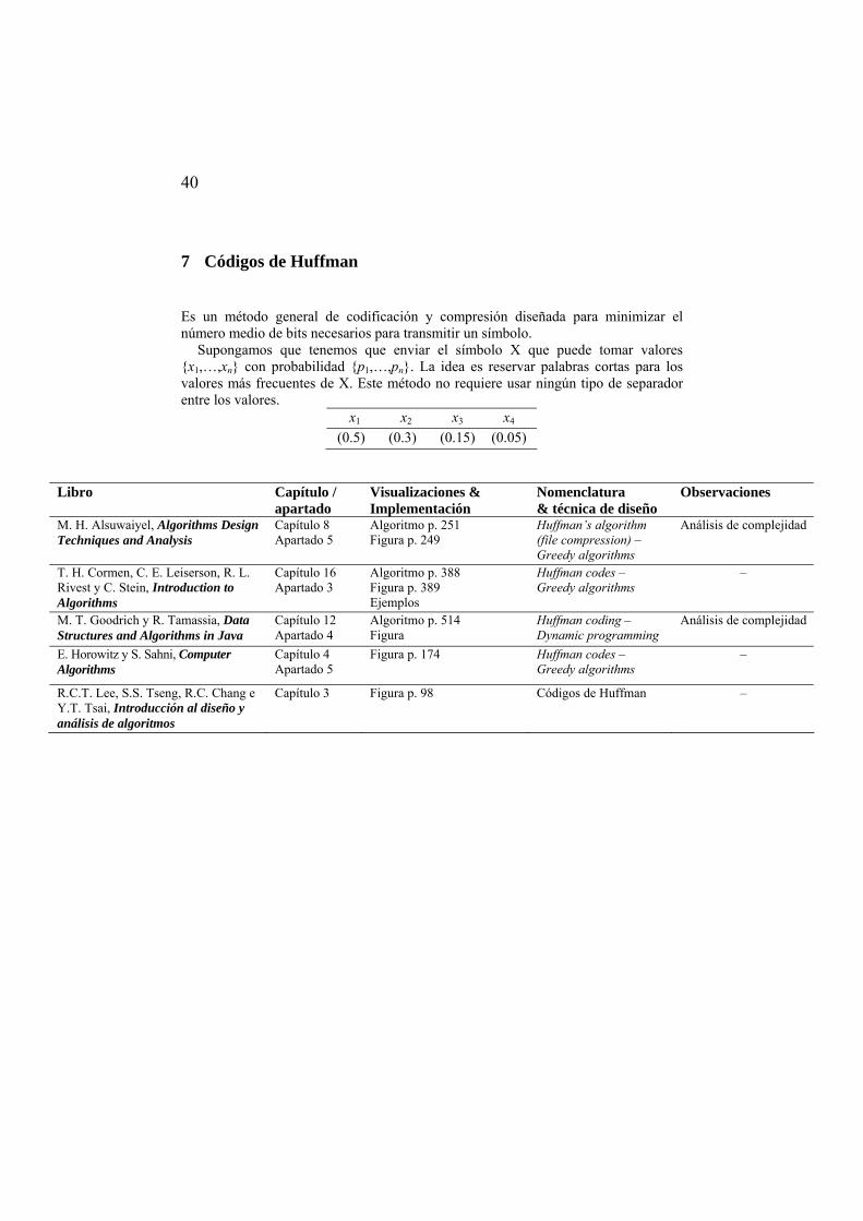
7 Códigos de Huffman

Es un método general de codificación y compresión diseñada para minimizar el número medio de bits necesarios para transmitir un símbolo.

Supongamos que tenemos que enviar el símbolo X que puede tomar valores {x1,…,xn} con probabilidad {p1,…,pn}. La idea es reservar palabras cortas para los valores más frecuentes de X. Este método no requiere usar ningún tipo de separador entre los valores.

x1 x2 x3 x4

(0.5) (0.3) (0.15) (0.05)




Observaciones




Huffman’s algorithm (file compression) – Greedy algorithms




Algoritmo p. 388 Figura p. 389 Ejemplos

Huffman codes – Greedy algorithms

–



Algoritmo p. 514 Figura

Huffman coding – Dynamic programming




Figura p. 174 Huffman codes – Greedy algorithms

–


Capítulo 3 Figura p. 98 Códigos de Huffman –

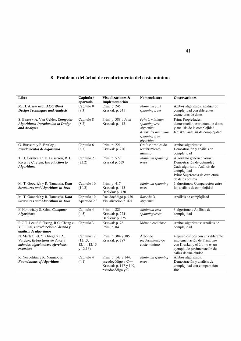
41

8 Problema del árbol de recubrimiento del coste mínimo



Nomenclatura Observaciones


Capítulo 8 (8.3)

Prim: p. 245 Kruskal: p. 241

Minimum cost spanning trees

Ambos algoritmos: análisis de complejidad con diferentes estructuras de datos


Capítulo 8 (8.2)

Prim: p. 388 y Java Kruskal: p. 412

Prim’s minimum spanning tree algorithm Kruskal’s minimum spanning tree algorithm

Prim: Propiedades, demostración, estructura de datos y análisis de la complejidad Kruskal: análisis de complejidad


Capítulo 6 (6.3)

Prim: p. 221 Kruskal: p. 220

Grafos: árboles de recubrimiento mínimo

Ambos algoritmos: Demostración y análisis de complejidad


Capítulo 23 (23.2)

Prim: p. 572 Kruskal p. 569

Minimum spanning trees

Algoritmo genérico voraz: Demostración de optimidad Cada algoritmo: Análisis de complejidad Prim: Sugerencia de estructura de datos óptima


Capítulo 10 (10.2)

Prim: p. 417 Kruskal: p. 413 Barůvka: p. 420


3 algoritmos: Comparación entre los análisis de complejidad



Pseudocódigo p. 420 Visualización p. 421

Baruvka’s algorithm



Capítulo 4 (4.5)

Prim: p. 221 Kruskal: p. 224 Barůvka: p. 225

Minimum-cost spanning trees

3 algoritmos: Análisis de complejidad


Capítulo 3 Kruskal: p. 76 Prim: p. 84

Método codicioso Ambos algoritmos: Análisis de complejidad


Capítulo 12 (12.13, 12.14, 12.15 y 12.16)

Prim: p. 384 y 385 Kruskal: p. 387

Árbol de recubrimiento de coste mínimo

4 ejemplos: dos con una diferente implementación de Prim, uno con Kruskal y el último es un ejemplo de pavimentación de calles de una ciudad


Capítulo 4 (4.1)

Prim: p. 143 y 144, pseudocódigo y C++ Kruskal: p. 147 y 149, pseudocódigo y C++


Ambos algoritmos: Demostración y análisis de complejidad con comparación final

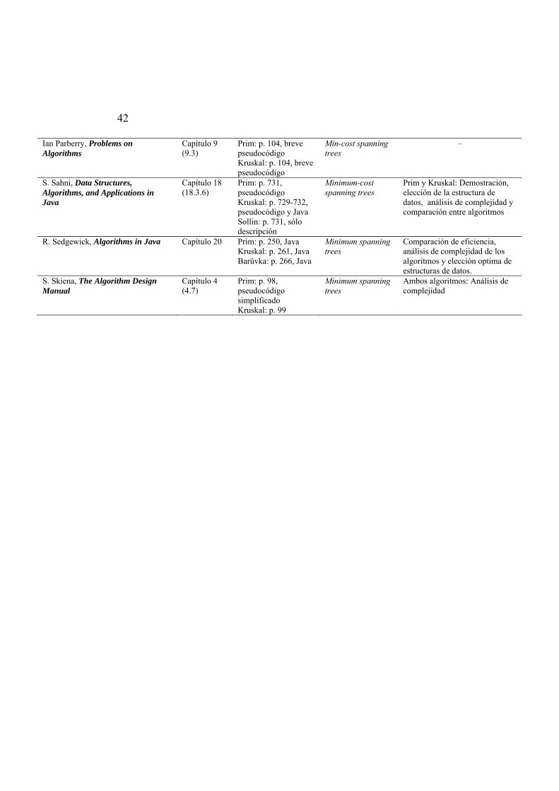
42


Capítulo 9 (9.3)

Prim: p. 104, breve pseudocódigo Kruskal: p. 104, breve pseudocódigo

Min-cost spanning trees

–


Capítulo 18 (18.3.6)

Prim: p. 731, pseudocódigo Kruskal: p. 729-732, pseudocódigo y Java Sollin: p. 731, sólo descripción

Minimum-cost spanning trees

Prim y Kruskal: Demostración, elección de la estructura de datos, análisis de complejidad y comparación entre algoritmos

R. Sedgewick, Algorithms in Java Capítulo 20 Prim: p. 250, Java Kruskal: p. 261, Java Barůvka: p. 266, Java


Comparación de eficiencia, análisis de complejidad de los algoritmos y elección optima de estructuras de datos.

S. Skiena, The Algorithm Design Manual

Capítulo 4 (4.7)

Prim: p. 98, pseudocódigo simplificado Kruskal: p. 99


Ambos algoritmos: Análisis de complejidad

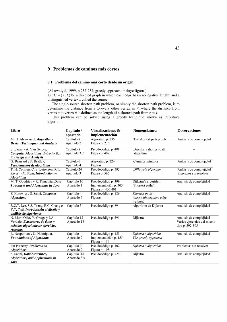
43

9 Problemas de caminos más cortos

9.1 Problema del camino más corto desde un origen

[Alsuwaiyel, 1999, p.232-237, greedy approach, incluye figuras] Let G = (V, E) be a directed graph in which each edge has a nonegative length, and a distinguished vertex s called the source.

The single-source shortest path problem, or simply the shortest path problem, is to determine the distance from s to every other vertex in V, where the distance from vertex s to vertex x is defined as the length of a shortest path from s to x.

This problem can be solved using a greedy technique known as Dijkstra’s algorithm.


Visualizaciones & implementación





The shortest path problem Análisis de complejidad




Dijkstra’s shortest-path algorithm

–



Algoritmo p. 224 Figuras

Caminos mínimos Análisis de complejidad




Dijkstra’s algorithm

Análisis de complejidad Ejercicios sin resolver



Pseudocódigo p. 399 Implementación p. 405 Figura p. 400-401

Dijkstra’s algorithm (Shortest paths)




Pseudocódigo p. 186 Figuras

Shortest-paths (case with negative edge weights)



Capítulo 3 Pseudocódigo p. 89 Algoritmo de Dijkstra Análisis de complejidad



Pseudocódigo p. 391 Dijkstra Análisis de complejidad Varios ejercicios del mismo tipo p. 392-395



Pseudocódigo p. 153 Implementación p. 155 Figura p. 154

Dijkstra’s algorithm The greedy approach





Dijkstra’s algorithm Problemas sin resolver




Dijkstra Análisis de complejidad

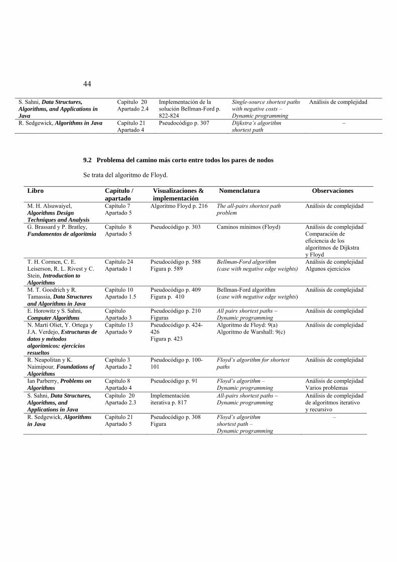
44



Implementación de la solución Bellman-Ford p. 822-824

Single-source shortest paths with negative costs – Dynamic programming


R. Sedgewick, Algorithms in Java Capítulo 21 Apartado 4

Pseudocódigo p. 307 Dijkstra’s algorithm shortest path

–

9.2 Problema del camino más corto entre todos los pares de nodos

Se trata del algoritmo de Floyd.


Visualizaciones & implementación




Algoritmo Floyd p. 216 The all-pairs shortest path problem




Pseudocódigo p. 303 Caminos mínimos (Floyd) Análisis de complejidad Comparación de eficiencia de los algoritmos de Dijkstra y Floyd




Bellman-Ford algorithm (case with negative edge weights)

Análisis de complejidad Algunos ejercicios




Bellman-Ford algorithm (case with negative edge weights)



Capítulo Apartado 3

Pseudocódigo p. 210 Figuras

All pairs shortest paths – Dynamic programming




Pseudocódigo p. 424-426 Figura p. 423

Algoritmo de Floyd: 9(a) Algoritmo de Warshall: 9(c)




Pseudocódigo p. 100-101

Floyd’s algorithm for shortest paths




Pseudocódigo p. 91 Floyd’s algorithm – Dynamic programming

Análisis de complejidad Varios problemas



Implementación iterativa p. 817

All-pairs shortest paths – Dynamic programming

Análisis de complejidad de algoritmos iterativo y recursivo

R. Sedgewick, Algorithms in Java


Pseudocódigo p. 308 Figura

Floyd’s algorithm shortest path – Dynamic programming

–

45


Busload of tourists [Baase, 2000, p.405, greedy algorithms] Given a collection of islands connected by one-way bridges, the bridges are of various lengths. The length of the bridge for edge uv is W (uv).

Imagine a busload of tourists all departing form a source vertex s at time zero. They spread out from s and walk at a uniform rate, say one meter per second (about 2.5 miles per hour, but using 2.5 requires more arithmetic). When they arrive at any new island (vertex) there are a lot of them, and they divide up, with some taking each bridge (edge) leaving that island, clearly, the first tourists to arrive at any island have followed a shortest path. In this example “shortest” can refer to time or distance.

Consider the situation when tourists are first arriving at vertex z. suppose they are traversing an edge yz, then a shortest path form s to z goes through, consists of a shortest path from s to y, followed by the edge yz.

Problema de la tabla de distancias entre ciudades [Gonzalo Arroyo, 2000, p.44-46, algoritmos voraces] Un cartógrafo acaba de terminar el plano de su país, que incluye información sobre las carreteras que unen las principales ciudades y sus longitudes. Ahora quiere añadir una tabla en la que se recoja la distancia entre cada par de ciudades del mapa (entendiendo por distancia la longitud del camino mas corto entre las dos). Escribir un algoritmo que le permita realizar esa tabla.

Single-source shortest paths [Sahni, 2000, p.721-726, greedy method, incluye figura y algoritmo] In this problem we are given a weighted graph G with the property that each edge (i,j) has a nonnegative cost (or length) a[i][j]. The length of a path is the sum of the costs of the edges on the path. He number on each edge is its cost. The length of the path 1, 2, 5 from vertex 1 to vertex 5 is 4+5=9; the length of the path 1, 5 is 8; and the length of the path 1,3,4,5 is 6

In the single-source, all-destinations, shortest-path problem, we must fund a shortest path from a given source vertex to each of the vertices (called destinations) in the graph to which there is a path, these paths are listed in increasing order of length, The number preceding each path is its length.

46

10 Problemas de grafos

Problema de recubrimiento de vértices de un grafo [Gonzalo Arroyo, 2000, p. 49-51, algoritmos voraces] Un recubrimiento R de vértices de un grafo no dirigido G= (V, A) es un conjunto de vértices tales que cada arista del grafo incide en, al menos, un vértice de R.

Diseñar un algoritmo que, dado un grafo no dirigido, calcule un recubrimiento de vértices de tamaño mínimo.

Problem 472 [Parberry, 1995, p. 110, greedy algorithms] The vertex cover problem is defined as follows. Let G = (V,E) be an undirected graph. A vertex cover of G is a set U⊆V such that for each edge (u,v)∈E, either u∈U or v∈U. A minimum vertex cover is a vertex cover with the smallest number of vertices in it. The following is a greedy algorithm for this problem:

function cover(V,E) 1. U := φ 2. repeat 3. let v ∈ V be a vertex of maximum degree 4. U := U ∪ {v}; V := V − {v} 5. E := E − {(u,w) such that u = v or w = v} 6. until E = φ 7. return(U)

Does this algorithm always generate a minimum vertex cover? Justify your answer.

Topological sorting [Sahni, 2000, p.712-716, greedy method, incluye figura] Often a complex Project may be decomposed into a collection of simpler tasks with the property that the completion of all these tasks implies that the Project has been completed.

For example, the automobile-assembly Project may be decomposed into these tasks: place chassis on assembly line, mount axles, mount wheels onto axles, fit seats onto chassis, paint, install brakes, install doors, and so on. A precedence relation exists between certain pairs of tasks. For example, the chassis must be placed on the assembly line before we can mount the axles. The set of tasks together with the precedence may be represented as a digraph- called an activity on vertex (AOV) network. The vertices of this digraph represent the tasks, and the directed edge (i,j) demotes the following precedence: task i must complete before task j can start.

The edge (1,4) implies that task 1 is to be done before task 4. Similarly, the edge (4,6) implies that task 4 is to be done before task 6. The edges (1,4) and (4,6) together

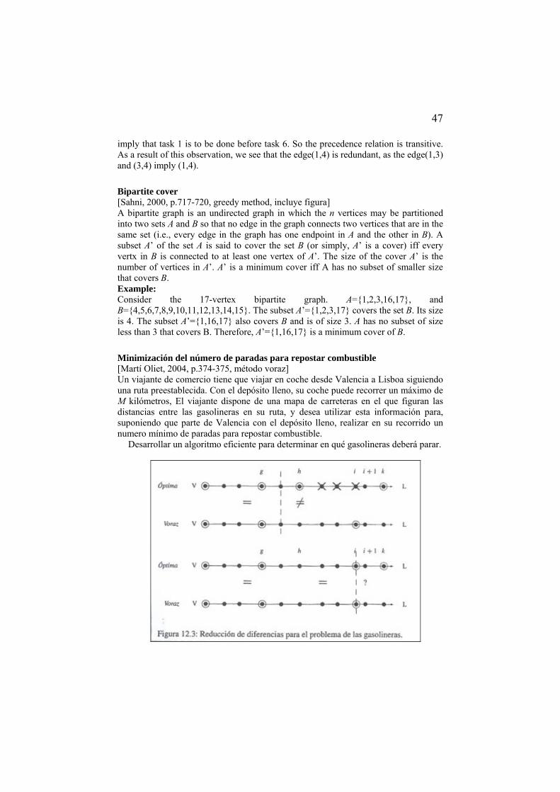
47

imply that task 1 is to be done before task 6. So the precedence relation is transitive. As a result of this observation, we see that the edge(1,4) is redundant, as the edge(1,3) and (3,4) imply (1,4).

Bipartite cover [Sahni, 2000, p.717-720, greedy method, incluye figura] A bipartite graph is an undirected graph in which the n vertices may be partitioned into two sets A and B so that no edge in the graph connects two vertices that are in the same set (i.e., every edge in the graph has one endpoint in A and the other in B). A subset A’ of the set A is said to cover the set B (or simply, A’ is a cover) iff every vertx in B is connected to at least one vertex of A’. The size of the cover A’ is the number of vertices in A’. A’ is a minimum cover iff A has no subset of smaller size that covers B. Example: Consider the 17-vertex bipartite graph. A={1,2,3,16,17}, and B={4,5,6,7,8,9,10,11,12,13,14,15}. The subset A’={1,2,3,17} covers the set B. Its size is 4. The subset A’={1,16,17} also covers B and is of size 3. A has no subset of size less than 3 that covers B. Therefore, A’={1,16,17} is a minimum cover of B.

Minimización del número de paradas para repostar combustible [Martí Oliet, 2004, p.374-375, método voraz] Un viajante de comercio tiene que viajar en coche desde Valencia a Lisboa siguiendo una ruta preestablecida. Con el depósito lleno, su coche puede recorrer un máximo de M kilómetros, El viajante dispone de una mapa de carreteras en el que figuran las distancias entre las gasolineras en su ruta, y desea utilizar esta información para, suponiendo que parte de Valencia con el depósito lleno, realizar en su recorrido un numero mínimo de paradas para repostar combustible.

Desarrollar un algoritmo eficiente para determinar en qué gasolineras deberá parar.

48

Problema de minimización de calles a pavimentar [Martí Oliet, 2004, p.381-383, método voraz] Los residentes de Barro City son demasiado tacaños para pavimentar las calles de la ciudad; después de todo, a nadie le gusta pagar impuestos. Sin embargo, tras varios meses de lluvias intensas empiezan a estar cansados de enfangarse los pies cada vez que salen a ala calle. Debido a su gran tacañería, en vez de pavimentar todas las calles de la ciudad, quieren pavimentar solamente las suficientes para poder ir de una intersección a otra cualquiera de la ciudad siguiendo una ruta pavimentada y, además, quieren gastarse tan poco dinero como sea posible en la realización de esta obra. Y es que a los residentes de Barro City no les importa caminar mucho, si ello les permite ahorrar algún dinero. El alcalde tiene interés en saber qué calles tienen que pavimentar para ajustarse al presupuesto.

Exercises 39 [Sahni, 2000, p.741, greedy method] Let t be a tree (not necessarily binary) in which a length is associated with each edge. Let s be a subset of the vertices of t and let t/S denote the forest that results when the vertices of S are detected form T. We wish to find a minimum-cardinality subset S such that no forest in T/S has a root-to-leaf path whose length exceeds d.

Develop a greedy algorithm to find a minimum-cardinality S (hint: start at the leaves and move toward the root.)

Prove the correctness of your algorithm. What is the complexity of your algorithm? In case it is not linear in the number of

vertices in T, redesign your algorithm so that its complexity is linear.

The bin packing problem [Alsuwaiyel, 1999, p.397-398, approximation algorithms] Given a collection of items u1, u2,..., un of sizes s1, s2,..., sn where each sj is between 0 and 1, we are required to pack these items into the minimum number of bins of unit capacity. We list her four heuristics for the BIN PACKING problem. • First Fit (FF). In this method, the bins are indexed as 1,2,... all bins are initially

empty. The items are considered for packing in the order u1, u2,..., un. To pack item ui, find the least index j such that bin j contains at most 1- si, and add item ui to the items packed in bin j.

• Best Fit (BF). This method is the same as same the FF method except that when item ui is to be packed, we look for that bin, which is filled to level l≤ 1- si and l is as large as possible.

• First Fit Decreasing (FFD): In this method, the items are first ordered by decreasing order of size, and then packed using the FF method.

• Best Fit Decreasing (BFD). In this method, the items are first ordered by decreasing order of size, and then packed using the BF method.

Bin packing [Cormen, 2001, p.1049-1050, approximation algorithms] Suppose that we are given a set of n objects, where the size Si of the ith object satisfies 0<Si<1.

49

We wish to pack all the objects into the minimum number of unit-size bins. Each bin can hold any subset of the objects whose total size does not exceed 1. a. Prove that the problem of determining the minimum number of bins required is

NP-hard. The first-fit heuristic takes each object in turn and places it into the first

bin that can accommodate it. Let S=∑=

n

iSi

1 . b. Argue that the optimal number of bins required is at least [S]. c. Argue that the first-fit heuristic leaves at most one bin less than half full. d. Prove that the number of bins used by the first-fit heuristic is never more than

[2S]. e. Prove an approximation ratio of 2 for the first-fit heuristic. f. Give an efficient implementation of the first-fit heuristic, and analyze its running

time.

Planar graph coloring [Alsuwaiyel, 1999, p. 395, approximation algorithms] Let G= (V, E) be a planar graph. By the Four Color Theorem, every planar graph is four-colorable. It is fairly easy to determine whether a graph is 2-colorable or not. On the other hand, to determine whether it is 3-colorable is NP-complete. Given an instance I of G, an approximation algorithm A may proceed as follows. Assume G is nontrivial, i.e., it has at least one edge. Determine if the graph is 2-colorable. If it is, then output 2; otherwise output 4. If G is 2- colorable, then |A(I)-OPT(I)|=0. If it is not 2-colorable, then |A(I)-OPT(I)|≤1.This is because in the latter case, G is either 3-colorable or 4-colorable.

Graph coloring [Baase, 2000, p. 581, approximation algorithms, incluye figures y algoritmo]

Coloreado de un grafo [Brassard & Bratley, 1996, p. 526-528, algoritmos heurísticos aproximados, incluye figuras] Sea G un grafo no dirigido, y sea n un entero. Un coloreado de G es una asignación de colores a los nodos de G de tal manera que dos nodos cualesquiera que estén conectados por una arista sean siempre de diferentes colores. Si no utiliza más de k colores diferentes, entonces es un coloreado k. El menor k tal que existe un coloreado k del gafo se llama número cromático del grafo, y cualquier coloreado k de estos será un coloreado óptimo. Definimos los cuatro problemas siguientes: • Dado un grafo G, ¿se puede colorear G con 3 colores? • Dado un grafo G y un entero k ¿se puede colorear G con k colores? • Dado un grafo G, hallar el numero cromático de G. • Dado un grafo G, hallar un coloreado optimo de G.

Planar Graph coloring [Horowitz & Sahni, 1978, p. 562-563, approximation algorithms, incluye algoritmo]

50

The Euclidean traveling salesman problem [Alsuwaiyel, 1999, p. 399-401, approximation algorithms, incluye figura] Given a set S of n points in the plane, find a tour Γ on these points of shortest length, Here, a tour is a circular path that visits every point exactly once, This problem is a special case of the traveling salesman problem, and is commonly referred to as the Euclidean Minimum Spanning Tree (EMST), whish is known to be NP-hard.

Let p1 be an arbitrary starting pint. An intuitive method would proceed in a greedy manner, visiting first that point closest to p1, say p2, and then that point which is closest to p2, and so on. This method is referred to as the Nearest Neighbor (NN) heuristic, and it can be shown that it does not result in a bounded performance ratio, i.e, RNN=infinity.

The traveling salesperson problem [Baase, 2000, p. 589, approximation algorithms, incluye figura]

El viajante [Brassard & Bratley, 1996, p. 528-529, algoritmos heurísticos aproximados] Conocemos las distancias entre un cierto número de ciudades. El viajante desea salir de una de estas ciudades, para visitar todas las demás ciudades exactamente una vez y volver al punto de partida habiendo recorrido la menor distancia posible. Suponemos que la distancia entre dos ciudades nunca es negativa.

El problema se puede representar como un grafo completo no dirigido con n nodos, nuestro problema, por tanto, requiere que hallamos un ciclo más corto y que pase por todos los nodos exactamente una vez de un grafo dado.

The travelling salesperson problem [Horowitz & Sahni, p. 231-234, approximation algorithms, incluye figura]

Un algoritmo de aproximación para el problema del agente viajero versión euclidiana [Lee, 2005, p. 395-397, algoritmos de aproximación, incluye figuras]

The vertex cover problem [Alsuwaiyel, 1999, p. 401-402, approximation algorithms] Recall that a vertex cover C in a graph G=(V,E) is a set of vertices such that each edge in E is incident to at least one vertex in C.

The problem of deciding whether a graph contains a vertex cover of size k, where k is a positive integer, is NP-complete. It follows that the problem of finding a vertex cover of minimum size is NP-hard.

The vertex-cover problem [Cormen, 2001, p. 1024, approximation algorithms, incluye figuras]

51

Un algoritmo de aproximación para el problema de cubierta de nodos [Lee, 2005, p. 393, algoritmos de aproximación, incluye dibujo y pseudocódigo]

Vertex cover [Skeina, 1998, p. 149, heuristic method, incluye figuras]

Minimizar el número medio de comparaciones necesarias para realizar una búsqueda [Martí Oliet, 2004, p.4 14-417, programación dinámica] Sean c1<c2<...<cn un conjunto de claves distintas ordenadas, y sea pi la probabilidad con que se pide buscar la clave ci y su información asociada, para i entre 1 y n. Se desea encontrar un árbol de búsqueda que minimice el numero medio de comparaciones necesarias para realizar una búsqueda, suponiendo que es decir

∑=

n

i ip1

=1, que todas las peticiones se refieren a claves que están en el árbol.

Calcular el coste mínimo entre cada par de vértices [Martí Oliet, 2004, p. 424-426, programación dinámica] Dado un grafo dirigido cuyas aristas están valoradas con números positivos, desarrollar algoritmos para: (a) calcular el coste (del camino) mínimo entre cada para de vértices del grafo, (b) calcular el numero de caminos de coste mínimo para cada par de vértices del

grafo, y (c) calcular la clausura reflexiva y transitiva de la relación dad por el grafo.

Problema de encontrar el camino de anchura máximo que une cada par de isla [Martí Oliet, 2004, p. 426-428, programación dinámica] Un archipiélago consta de unas cuantas islas y varios puentes que unen ciertos pares de islas.

Para casa puente (que puede ser de dirección única), además de saber la isla origen y la isla destino, se conoce su anchura>0. La anchura de un camino formado por una sucesión de puentes es la anchura mínima entre las anchuras de todos los puentes que lo forman. Para cada par de islas de desea saber cuál es el camino de anchura máxima que las une (siempre que exista alguno).

Multistage graphs [Horowitz & Sahni, 1978, p. 203-208, dynamic programming, incluye algoritmo y figura] A multistage graph G=(V,E) is a directed graph in which the vertices are partitioned into k≥ 2 disjoint sets Vi, 1≤i≤k. In addition, if <u,v> is an edge in E then u∈Vi and v∈Vi+1 for some i, 1≤i<k.

The sets V1 and Vk are such that | V1|=| Vk|=1. Let s and t respectively be the vertex in V1 and Vk. S is the source and t the sink. Let c(i,j) be the cost of edge <i,j>.

52

The cost of a path from s to t is the sum of the costs of the edges on the path. The multistage graph problem is to find a minimum cost path from s to t. Each set Vi defines a stage in the graph. Because of the constraints on E, every path from s to t starts in stage 1, goes to stage 2, then to stage 3, then to stage 4 etc. and eventually terminates in stage k.

El problema del árbol binario optimo [Lee, 2005, p. 283-291, programación dinámica, incluye figuras] Dados n identificadores a1<a2<a3…<an, pueden tenerse muchos árboles binarios distintos. Por ejemplo, suponga que es necesario encontrar un árbol binario óptimo para cuatro identificados: 1, 2, 3 y 4. Aplicando la programación dinámica se encuentran cuatro árboles binarios con el coste mínimo.

Search Binary Tree [Neapolitan, 1997, p. 115-120, dynamic programming] Problem: Determine the node containing a key in a binary search tree. It is assumed that the key is in the tree. Inputs: A pointer tree to a binary search tree and a key keyin. Outputs: A pointer p to the node containing the key.

Optimal Binary Search Tree [Neapolitan, 1997, p. 120-121, dynamic programming] Problem: Determine an optimal binary search tree for a set of keys, each with a given probability of being the search key. Inputs: n, the number of keys, and an array of real numbers p indexed from 1 to n, where p[i] is the probability of searching for the ith key. Outputs: A variable minavg, whose value is the average search time for an optimal binary search tree; and a two-dimensional array R from which an optimal tree can be constructed. R has its rows indexed from 1 to n + 1 and its columns indexed from 0 to n. R[i][j] is the index of the key in the root of an optimal tree containing the ith through the jth keys.

Build Optimal Binary Search Tree [Neapolitan, 1997, p. 121-123, dynamic programming] Problem: Build an optimal binary search tree. Inputs: n, the number of keys, an array Key containing the n keys in order, and the array R. R[i][j] is the index of the key in the root of an optimal tree containing the ith through the jth keys. Outputs: a pointer tree to an optimal binary search tree containing the n keys.

El problema ponderado de búsqueda de bordes en una gráfica en un solo paso [Lee, 2005, p. 301-309, programación dinámica, incluye figuras] Dado un grafo no dirigido simple G=(V, E) donde cada vértice v∈V está asociado con un peso wt(v). Todos los bordes de G tienen la misma longitud.

53

Se supone que en alguna arista de G está escondido un fugitivo que puede moverse a cualquier velocidad. En cada arista de G, para buscar al fugitivo se asigna un buscador de aristas. El buscador siempre empieza desde un vértice. El costo de recorrer una arista (u,v) se define como wt(u) si el buscador empieza desde u y como wt(v) si empieza desde v. suponga que todos los buscadores de aristas se desplazan a la misma velocidad. El problema ponderado de búsqueda de aristas en una grafica simple en un solo paso consiste en disponer las direcciones de búsqueda de los buscadores de aristas de modo que el fugitivo sea atrapado en un paso y se minimice el número de buscadores utilizados.

Moving on a checkerboard [Cormen, 2001, p. 368, dynamic programming] Suppose that you are given an n × n checkerboard and a checker. You must move the checker from the bottom edge of the board to the top edge of the board according to the following rule. At each step you may move the checker to one of three squares: 1. The square immediately above, 2. The square that is one up and one to the left (but only if the checker is not already

in the leftmost column), 3. The square that is one up and one to the right (but only if the checker is not

already in the rightmost column). Each time you move from square x to square y, you receive p(x, y) dollars. You are

given p(x,y) for all pairs (x, y) for which a move from x to y is legal. Do not assume that p(x, y) is positive.

Give an algorithm that figures out the set of moves that will move the checker from somewhere along the bottom edge to somewhere along the top edge while gathering as many dollars as possible. Your algorithm is free to pick any square along the bottom edge as a starting point and any square along the top edge as a destination in order to maximize the number of dollars gathered along the way. What is the running time of your algorithm?

Problema de planificación de la un viaje [Martí Oliet, 2004, p. 428-430, programación dinámica] Indian Pérez quiere planificar una aventurilla por el Amazonas. A lo largo del río hay n poblados indígenas, cuyos habitantes, al observar el creciente auge del turismo rural, han ideado un sistema de alquiler de canoas. En cada poblado se puede alquilar una canoa, la cual puede devolverse en cualquier otro poblado que este a favor de la corriente. Consultando por Internet los costes de alquileres entre poblados, Indiana ha constatado que el coste del alquiler desde un poblado i hasta otro j puede resultar mayor que el coste total de una serie de alquileres más breves. En tal caso, es más rentable devolver la primera canoa en alguna aldea k entre i y j, y seguir camino en una segunda canoa, sin cargos adicionales por cambiar de canoa. (a) Dar un algoritmo eficiente para determinar el coste mínimo de un viaje en canoa

desde todos los posibles puntos de partida i hasta todos los posibles puntos de llegada j.

54

(b) Modificar el algoritmo de apartado anterior para que, además, proporciona un plan de alquileres para viajar desde el primer poblado (el mas cercano al nacimiento del río) hasta el ultimo (el mas cercano a al desembocadura).

Maximum bipartite matching [Goodrich, 2001, p. 430] A problem that arises in a number of important applications is the maximum bipartite matching problem. In this problem, we are given an undirected graph G= (V, E) such that the vertices of V are divided into two sets, X and Y, with V=X∪Y and every edge in E joining a vertex in X to a vertex in Y.

Such a graph is called a bipartite graph. A matching in G is a set of edges from E that have no endpoints in common-such a set “pairs” up vertices in X with vertices in Y so that each vertex has at most one “partner” in the other set. The maximum bipartite matching problem is to find a matching that has the greatest number of edges (over all legal matchings) Example: Let G=(V,E) be a bipartite graph with V= X ∪Y, where the set X represents a group of young men and the set Y represents a group of young women, who are all together at community dance. Let there be an edge joining x in X and y in Y if x and y are willing to dance with one another.

A maximum matching in G corresponds to a largest set of compatible pairs of men and women who can all be happily dancing at the same time.

55

11 Otros problemas

Problema de 2 terminales (uno a cualquiera/uno a muchos) [Lee, 2005, p. 103-108, método codicioso, incluye figuras] El problema de direccionamiento de un canal se trata de dos terminales donde cada Terminal marcada de un renglón superior debe conectarse o unirse con un terminal de un renglón inferior de manera uno a uno.

Se requiere que ningún par de líneas se corte. Además todas las líneas son verticales u horizontales. Toda línea horizontal corresponde a una pista.

El problema del mínimo de guardias cooperativos para polígonos de 1-espiral resuelto por el método codicioso [Lee, 2005, p. 108-113, método codicioso, incluye figures y algoritmo] El problema del mínimo de guardias cooperativos es una variante del problema de la galería de arte, que se define como sigue. Se tiene un polígono, que representa la galería de arte, y se requiere colocar el número mínimo de guardias en el polígono de modo que cada punto del polígono sea visible por lo menos para un guardia.

El problema de la galería de are es un problema NP-hard.

Problema de la línea [Martí Oliet, 2004, p. 358-359, método voraz] Dado un conjunto {r1, r2,…, rn} de puntos de la recta real, determinar el menor conjunto de intervalos cerrados de longitud 1 que contenga a todos los puntos dados.

The subset-sum problem [Alsuwaiyel, 1999, p. 408, approximation algorithms, incluye Pseudocódigo]

El campeonato mundial [Brassard & Bratley, p. 293-295, programación dinámica, incluye figura] Considere una competición en la cual hay dos equipos A y B que juegan un máximo de 2n-1 partidas, y en donde el ganador es el primer equipo que consiga n victorias. Suponemos que no hay empates, que los resultados de todos los partidos son independientes, y que para cualquier partido dado hay una probabilidad constante p de que el equipo A sea el ganador, y por tanto una probabilidad constante q=1-p de que gane el equipo B.

Sea P(i,j) la probabilidad de que el equipo A gane el campeonato, cuando todavía necesitan i victorias más para conseguirlo, mientras que el equipo B necesita j victorias más para ganar. Por ejemplo, antes del primer partido del campeonato la probabilidad de que gane el equipo A es P(n,n): ambos equipos necesitan todavía n victorias para ganar el campeonato. Si el equipo A necesita cero victorias más, entonces lo cierto es que ya han ganado el campeonato, y por tanto P(0,i)=1, con 1≤i≤n.

56

De manera similar, si el equipo B necesita 0 victorias más, entonces ya han ganado el campeonato, y por tanto P(i,0)=1, con 1≤i≤n. como no puede producirse una situación en la que ambos equipos hayan ganado todos los partidos que necesitaban, p(0,0) carece de significado.

Por último dado que el equipo A gana cualquier partido con una probabilidad p y pierde con una probabilidad q:

P(i,j)=pP(i-1,j)+qP(i,j-1), i≥1,j≥1 Calcular P(i,j)

The subset-sum problem [Cormen, 2001, p. 1043-1049, approximation algorithms] An instance of the subset-sum problem is a pair (S, t), where S is a set {x1, x2, ..., xn} of positive integers and t is a positive integer. This decision problem asks whether there exists a subset of S that adds up exactly to the target value t. This problem is NP-complete.

Problema rectilíneo de m-centros [Lee, 2005, p. 417-423, algoritmos de aproximación, incluye figures y algoritmo] Dado un conjunto de n puntos en el plano, el problema de m-centros consiste en encontrar m cuadrados rectilíneos que cubran todos estos n puntos de modo que la longitud del lado máximo de estos cuadrados se minimice. Por cuadrado rectilíneo se entiende un cuadrado con lados perpendiculares o paralelos al eje x del plano euclidiano.

Debido a que los cuadrados rectilíneos menores pueden agrandarse en una solución para el problema rectilíneo del m-centros sin afectar nuestro objetivo, se supone que todos los m cuadrados rectilíneos de una solución tienen la misma longitud.

Reliability design [Horowitz & Sahni, p. 228-230, dynamic programming, incluye figura] The problem is to design a system which is composed of several devices connected in series. Let ri be the reliability of device Di (i.e. ri is the probability that device i will function properly). Then, the reliability of the entire system is ∏ ri. Even if the individual devices are very reliable (the ri’s are very close to one), the reliability of the system may not be very good.

For example, if n=10 and ri =99, 1≤i≤10 then ∏ ri=904. Hence, it is desirable to duplicate devices. Multiple copies of the same device type

are connected in parallel through the use of switching circuits. The switching circuits determine which devices in any given group are functioning

properly. Then make use of one such device at each stage.

Problema de apareamiento del máximo de par de bases de ARN [Lee, 2005, p. 270-282, programación dinámica, incluye algoritmo y tabla] El acido ribonucleico (ARN) es una cadena simple de nucleótidos (bases), adenina (A), guanina (G), citosina (C) y uracil (U). La secuencia de las bases A, G, C y U se denomina estructura primaria de un ARN.

57

En el ARN, G y C pueden formar un para de bases G≡C mediante un triple enlace de hidrogeno. A y U pueden formar un para de bases A=U mediante un doble enlace de hidrogeno, y G y U pueden formar una para de bases G-U mediante un enlace simple de hidrogeno. Debido a estos enlaces de hidrogeno, la estructura primaria de un ARN puede plegarse sobre si misma para formar su estructura secundaria. Por ejemplo, suponga que se tiene la siguiente secuencia de ARN.

A-G-G-C-C-U-U-C-C-U Así, esta estructura puede plegarse sobre si misma para formar muchas estructuras

secundarias posibles, en la naturaleza, no obstante, sólo existe una secuencia secundaria correspondiente a una secuencia de ARN.

El objetivo de la predicción de la estructura secundaria es encontrar una estructura secundaria que tenga la energía libre mínima.

Problema de la distribución del botín a medias sin desempaquetar las cajas [Martí Oliet, 2004, p. 408-410, programación dinámica] El Maqui y el Popeye acaban de desvalijar la reserva nacional de oro. Los lingotes están empaquetados en n cajas de diferentes pesos naturales positivos pi para i entre 1 y n. como no tienen tiempo de desempaquetarlos para dividir el botín, deciden utilizar los pesos de cada una de las cajas para distribuir el botín a medias. Al cabo de un buen rato todavía no han conseguido repartirse el botín, por lo cual acuden al Teclas para saber si el botín se puede dividir en dos partes iguales sin desempaquetar las cajas con los lingotes.

Problema de cálculo de probabilidad del éxito de un equipo [Martí Oliet, 2004, p. 410-411, programación dinámica] Consideramos una competición entre dos equipos, A y B, en la que el ganador es el primer equipo que consiga n victorias. Suponemos que no hay empates, que los resultados de todos los partidos son independientes, y que para cualquier partido dado hay una probabilidad constante p de que lo gane el equipo A (por tanto una probabilidad constante q=1-p de que lo gane el equipo B). (a) Desarrollar un algoritmo para calcular, antes del primer partido, la probabilidad

de que el equipo A gane la competición. (b) Hacer lo mismo cuando existe una probabilidad p de que A gane un partido, q

de que lo pierda, y r (con p+q+r=1) de que haya empate. Un empate no supone una victoria para ningún equipo y siguen siendo necesarias n victorias para ganar la competición.

La cantidad de unidades enviadas desde un almacén [Martí Oliet, 2004, p. 442-443, programación dinámica] Se tienen dos almacenes A1 y A2 en los que se dispone respectivamente de a1 y a2 unidades (indivisibles) de un determinado producto. Desde estos dos almacenes se ha de abastecer a n comercios c1,... ,cn, en cada uno de los cuales se precisa una determinada cantidad cj (para j entre 1 y n) de unidades del producto, de forma que

∑ =

n

j jc1

= a1+a2. El coste del transporte desde Ai hasta cj viene dado por una función

tij (x) donde x es el número de unidades del producto transportadas.

58

Se desea determinar las cantidades de unidades xij que cada almacén debe enviar a cada comercio de forma que el coste total del transporte ∑ij ijt (xij) sea mínima.

Problema de maximizar la cantidad de comida de las vacas [Martí Oliet, 2004, p. 444-447, programación dinámica, incluye figuras de recipientes y tablas] El Tío Antonio tiene en su granja dos vacas: Devoradora y Listilla. Antes de ordeñarlas las alimenta llenando una hilera de n cubos con pienso (n es par). Cada cubo i (para i entre 1 y n) contiene una cantidad pi de pienso indicada en el cubo (todas las cantidades son distintas). Cada vaca en su turno debe elegir el cubo de uno de los extremos y comerse su contenido. El cubo se retira y el turno pasa a la otra vaca. Se sigue así hasta agotar los cubos. La vaca que comienza comiendo se determina a priori por un procedimiento cualquiera. El objetivo de ambas vacas es comer en total lo máximo posible. La estrategia de Devoradora consiste en pensar poco y escoger el cubo de los extremos que este más lleno. En cambio, Listilla prefiere pensárselo un poco más, para lo que ha adquirido lo ultimo en computadoras vacunas portátiles. (a) Demostrar que la estrategia de Devoradora no es optima, incluso cuando le toca

escoger primero. (b) Listilla ha cursado un master en informática por la escuela superior Bovina,

pero en dicha escuela no estudian la programación dinámica, por lo que pide ayuda para diseñar un algoritmo utilizando dicha técnica, suponiendo que le toca empezar a escoger.

(c) Diseñar un algoritmo de coste lineal de forma que Listilla, siempre que comience comiendo ella, coma al menos tanto como Devoradora, independientemente de la estrategia que siga esta ultima. ¿Es óptima la nueva estrategia?

The Partition Problem [Skeina, 1998, p. 56-60, dynamic programming, incluye figuras] Suppose that three workers are given the task of scanning through a shelf of books in search of a given piece of information. To get the job done fairly and efficiently, the books are to be partitioned among the three workers. To avoid the need to rearrange the books or separate them into piles, it would be simplest to divide the shelf into three regions and assign each region to one worker.

But what is the fairest way to divide the shelf up? Input: A given arrangement S of non-negative numbers and an integer k. Output: Partition S into k ranges, so as to minimize the maximum sum over all the ranges. This so-called linear partition.

Minimum weight triangulation [Skeina, 1998, p. 64-65, dynamic programming, incluye figuras] A triangulation of a polygon p={v1, …, vn, v1} is a set of non-intersecting diagonals that partitions the polygon into triangles. We say that the weight of a triangulation is the sum of the lengths of its diagonals. Any given polygon may have many different

59

triangulations. For any given polygon, we seek to find its minimum weight triangulation. Triangulation is a fundamental component of most geometric algorithms.

Noncrossing subset of nets [Sahni, 2000, p. 825-828, dynamic programming, incluye figura] We are given a routing channel with n pins on either side and a permutation C. Pin i on the top side of the channel is to be connected to pin Ci on the bottom side, 1≤i≤n.

The pair (i,Ci) is called a net. In all we have n nets that are to be connected or routed. Suppose that we have two

or more routing layers of which one is a preferred layer. For example, in the preferred layer it may be possible to use much thinner wires, or the resistance in the preferred layer may be considerably less than in other layers. Our task is to route as many nets as possible in the preferred layer. The remaining nets will be routed, at least partially, in the other layers. Since two nets can be routed in the same layer if they do not cross, our task is equivalent to finding a maximum noncrossing subset (MSS) of the nets. Such a subset has the property that no two nets of the subset cross. Since net (i, ci) is completely specified by i, we may refer to this net as net i.

60

12 Conclusiones

Hemos presentado el resultado de un trabajo “hercúleo” de revisión bibliográfica. Con las carencias o inexactitudes que puede tener, consideramos que es un trabajo muy útil para profesores e investigadores. Queremos resaltar el análisis realizado de los problemas del primer grupo (problemas de planificación), que ha permitido organizarlos en 7 subgrupos de problemas relacionados. La clasificación resultante puede ser muy útil para el diseño o la ampliación de ayudantes interactivos [16,17], ya que presentan características similares. Por esta razón, se han incluido también las figuras con que se ilustran en los libros de texto revisados.

Hay varios trabajos futuros posibles. Por supuesto, el estudio es susceptible de ampliarse en los problemas menos analizados o con nuevos problemas o libros de texto. Asimismo, los resultados pueden utilizarse para nuestra línea de trabajo sobre ayudantes interactivos, sobre todo los problemas de planificación. Agradecimientos. Este trabajo se ha financiado con el proyecto TIN2008-04301/TSI del Ministerio de Innovación y Ciencia.

Referencias

1. M. H. Alsuwaiyel, 1999. Algorithms Design Techniques and Analysis, World Scientific 2. S. Baase y A. van Gelder, 2000. Computer Algorithms: Introduction to Design and Analysis 3. G. Brassard y P. Bratley, 1996. Fundamentos de algoritmia, Prentice-Hall 4. T. H. Cormen, C. E. Leiserson, R. L. Rivest y C. Stein, 2001. Introduction to Algorithms,

The MIT Press, 2ª ed. 5. J. Gonzalo Arroyo y M. Rodríguez Artacho, 2000. Esquemas algorítmicos enfoque

metodológico y problemas resueltos, UNED 6. M. T. Goodrich y R. Tamassia, 2001. Data Structures and Algorithms in Java, John Wiley &

Sons, 2ª ed. 7. E. Horowitz y S. Sahni, 1978. Fundamentals of Computer Algorithms, Pitman 8. R. C. T. Lee, S. S. Tseng, R. C. Chang e Y. T. Tsai, 2005. Introducción al diseño y análisis

de algoritmos, McGraw-Hill 9. N. Martí Oliet, Y. Ortega y J. A. Verdejo, 2004. Estructuras de datos y métodos

algorítmicos: ejercicios resueltos, Pearson 10. R. Neapolitan y K. Naimipour, 1997. Foundations of Algorithms, Jones and Bartlett 11. I. Parberry, 1995. Problems on Algorithms, Prentice Hall 12. S. Sahni, 2005. Data Structures, Algorithms, and Applications in Java, Silicon Press 13. R. Sedgewick, 2002. Algorithms in Java, Addison-Wesley 14. S. Skiena, 1998. The Algorithm Design Manual, Springer-Verlag 15. J. Á. Velázquez Iturbide, C. A. Lázaro Carrascosa, e I. Hernán Losada. “Asistentes

interactivos para el aprendizaje de algoritmos voraces”. En IEEE Revista Iberoamericana de Tecnologías del Aprendizaje, IEEE-RITA, 4(3):213-220, agosto 2009.

16. J. Á. Velázquez-Iturbide, y A. Pérez-Carrasco. “Active learning of greedy algorithms by means of interactive experimentation”. En Proc. 14th Annual Conf. on Innovation and Technology in Computer Science Education, ITiCSE 2009. ACM Press, pp. 119-123.

revisión bibliográfica de problemas combinatorios

Documents