control engineering group - universidad de sevilla · 2005-05-17 · – introduced by houpis and...
TRANSCRIPT

1
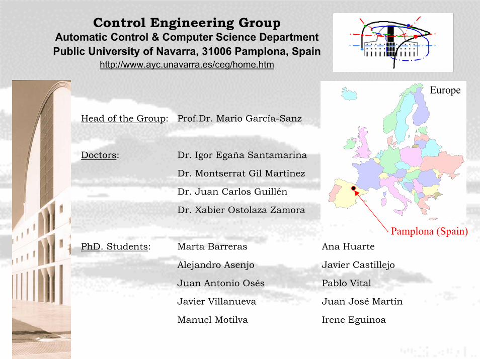
Control Engineering Group
Automatic Control & Computer Science DepartmentPublic University of Navarra
31006 Pamplona, Spain
http://www.ayc.unavarra.es/ceg/home.htm
2
Head of the Group: Prof.Dr. Mario García-Sanz
Doctors: Dr. Igor Egaña Santamarina
Dr. Montserrat Gil Martínez
Dr. Juan Carlos Guillén
Dr. Xabier Ostolaza Zamora
PhD. Students: Marta Barreras Ana Huarte
Alejandro Asenjo Javier Castillejo
Juan Antonio Osés Pablo Vital
Javier Villanueva Juan José Martín
Manuel Motilva Irene Eguinoa
Europe
Pamplona (Spain)
Control Engineering GroupAutomatic Control & Computer Science DepartmentPublic University of Navarra, 31006 Pamplona, Spain
http://www.ayc.unavarra.es/ceg/home.htm

3
With Prof. Isaac Horowitz, October 2000
Control Engineering GroupAutomatic Control & Computer Science DepartmentPublic University of Navarra, 31006 Pamplona, Spain
http://www.ayc.unavarra.es/ceg/home.htm
Basic Research on QFT Robust Control. +Applied Research Projects with Industry.
In the last 5 years: - More than 50 papers (Journals and Conf.) on QFT. - 7 Patents. - 5 Ph.D. Dissertations on QFT. - 6 Research Projects with Industry - 3 Research Projects supported by Spanish Gov. - 10 Ph.D Students working on QFT.
Guest Editor, Robust Frequency Domain Special Issue,Int. J. Robust Non-linear Control, Wiley, 2003.
Organizer of the 5th International Symposium onQuantitative Feedback Theory and Robust FrequencyDomain Methods, Pamplona, August 2001.
NATO Lecturer. (USA, Italy, Portugal, etc)5th QFT Symp., Pamplona, August 2001

M.TorresCompany
PublicUniversityof Navarra UR
CEIT
Aerospace Division
BoeingAirbus - A380 - Eurofighter - EurocopterNorthrop Gr.British Aerosp...
ControlEngineering
Group
Applied Research Projects
- Wastewater Treatment Plants- Drainage and Sewage Water Networks
Energy Division
Applied Research Projects- Wind Turbines Design- Aerospace Machinery- Paper Machinery
QFT Research- Fundamentals- MIMO Processes- Time-delay Systems- Distributed Plants- Non-linear Controllers
Paper Division
Tetra PakGeorgia Pacific
International Paper...
5
EXTERNAL DISTURBANCE REJECTION INUNCERTAIN MIMO SYSTEMSWITH QFT NON-DIAGONAL
CONTROLLERS
M. García-Sanz1, M. Barreras1, I. Egaña1, C.H. Houpis2
€
1Automatic Control and Computer Science Department,Public University of Navarra, 31006 Pamplona, SPAIN.
2Air Force Institute of Technology, Air Force ResearchLaboratory, Wright-Patterson AFB, Ohio, U.S.A.
http://www.ayc.unavarra.es/ceg/home.htmEmail: [email protected]
Authors wish to gratefully appreciate the support given by the Spanish “Ministerio de Ciencia yTecnología” (MCyT) under grants CICYT DPI’2000-0785 and DPI’2003-08580-C02-01.

6
• Disturbance attenuation in multivariable systems is often an importantand difficult problem to deal with.
• This work circumvents rejection of external disturbances in MIMOsystems with plant model uncertainties.
• The Quantitative Feedback Theory (QFT) is applied to design fullypopulated matrix controllers to attenuate the effect of externaldisturbances at plant input and plant output.
1.- Introduction

7
• The study starts with some previous ideas– suggested by Garcia-Sanz and Egaña (2002)– about the design of non-diagonal QFT controllers to reduce the loop
coupling in tracking problems,García-Sanz, M. and I. Egaña (2002). Quantitative Non-diagonalController Design for Multivariable Systems with Uncertainty.International Journal of Robust and Non-Linear Control. Nº 12, pp. 321-333. John Wiley & Sons.
• and considers the approach– introduced by Houpis and Rassmussen (1999)– about MIMO systems with external disturbances.
Houpis, C.H. and S. J. Rasmussen (1999). Quantitative Feedback TheoryFundamentals and Applications. Marcel Dekker, New York, ISBN: 0-8247-7872-3.

8
• Consider the n x n linear multivariable system shown in Fig.1.
2.- Rejection of External Disturbances at Plant Input
r = 0 -
’ d i
P di
d i
G
u v + y
d 0
+
’ d 0
P d 0
P + + Fig. 1 General structure of a MIMO
system with plant outputand input external disturbances.
• P is the plant, P є P and P is a set of possible plants due to uncertainty,• G is the full populated matrix controller,
• Pdi and Pdo are the plant input and output disturbance transfer functions.• di’ and do’ are the plant input and output external disturbances respectively.
=
=
nnnn
n
n
nnnn
n
n
g...gg............
g...ggg...gg
G;
p...pp............
p...ppp...pp
P
21
22221
11211
21
22221
11211

9
• denoting the external disturbance at plant input by
• then the output due to the external disturbance at plant input is,
• and the closed loop transfer matrix TY/di that relates the disturbance atplant input to the output y becomes,
'idii dPd =
( ) '//
1ididiYidiYi dPddy TTPGPI ==+= −
( ) PGPIT 1/
−+=diY
(1)
(2)
r = 0
-
’ d i
P di
d i
G
u v + y
d 0
+
’ d 0
P d 0
P + +

10
• Multiplying Eq.(2) by (I + P G),• pre-multiplying by• and denoting
where Λ is the diagonal part and B the balance of P-1 respectivelyand Gd is the diagonal part and Gb the balance of G respectively
• and rearranging it, yields the next expression
TY/di = ( I + Λ-1 Gd ) -1Λ-1 – ( I + Λ-1 Gd ) -1 Λ-1 [( B + Gb ) TY/di ]
1−P[ ]
bd
ij
GGGBPpP
+=
+Λ===− **1
(7)
[ ]
+
=+Λ===
0...p...0...
p...0
p000...000p
p*n
*n
*nn
*
1
111*ij
*1- BPP
+
=+=
0...g...0...
g...0
g000...000g
n
n
nn 1
111
bd GGG

11
the only part which has anon-diagonal structure. Itwill be call the couplingmatrix Cdi
• By inspecting Equation (7) two different terms can be found:
TY/di = ( I + Λ-1 Gd ) -1Λ-1 – ( I + Λ-1 Gd ) -1 Λ-1 [( B + Gb ) TY/di ] (7)
gii *
1
iip
ui0 yi
-
∑=
=n
i
dicd1
jijdi-j
* 1 ii p g ii
0 y i
-
u i
di i
1 ≤ i ≤ n
A diagonal termTY/di-d = ( I + Λ-1 Gd ) -1 Λ-1
(8) A non-diagonal termTY/di-b = ( I + Λ-1 Gd )-1 Λ-1 [(B+ Gb )TY/di](10)
12
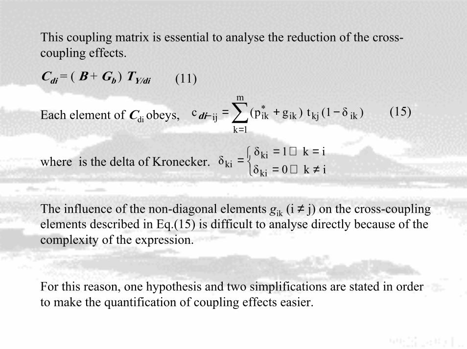
This coupling matrix is essential to analyse the reduction of the cross-coupling effects.
Cdi = ( B + Gb ) TY/di
Each element of Cdi obeys,
where is the delta of Kronecker.
The influence of the non-diagonal elements gik (i ≠ j) on the cross-couplingelements described in Eq.(15) is difficult to analyse directly because of thecomplexity of the expression.
For this reason, one hypothesis and two simplifications are stated in orderto make the quantification of coupling effects easier.
)δ(1t)gp(c ikkjik
m
1k
*ikij −+=∑
=−di
(11)
(15)
≠⇔==⇔=
=ik0δik1δ
δki
kiki

13
Hypothesis H1: The diagonal elements tjj in Eq. (15) are assumed to bemuch larger than the non-diagonal ones tkj,
( ) ( ) jkforgptgpt ik*ikkjij
*ijjj ≠+>>+
Simplification S1: Applying Hypothesis H1, Eq. (15) can be rewritten as,
ji;)gp(tc ij*ijjjij ≠+=−di
Simplification S2: The elements tjj can be replaced using the expressionobtained from the equivalent system in Eq. (8).
1*jjjj
1*jj
jj1
−
−
+=
pg
pt
14
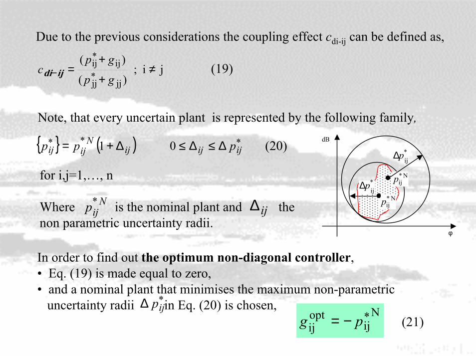
Due to the previous considerations the coupling effect cdi-ij can be defined as,
ji;)(
)(
jj*jj
ij*ij ≠
+
+=− gp
gpc ijdi (19)
In order to find out the optimum non-diagonal controller,• Eq. (19) is made equal to zero,• and a nominal plant that minimises the maximum non-parametric uncertainty radii in Eq. (20) is chosen,*
ijp∆N*
ijoptij pg −= (21)
N*ijp ij∆
Note, that every uncertain plant is represented by the following family,
{ } ( ) *ijijij
N*ij
*ij ppp ∆≤∆≤∆+= 01
for i,j=1,…, n
Where is the nominal plant and thenon parametric uncertainty radii.
(20) *ijp∆
N *ijp
*ijp∆
dB
φ
N *ijp
15
Effect ofoptimum
non-diagonalcontroller
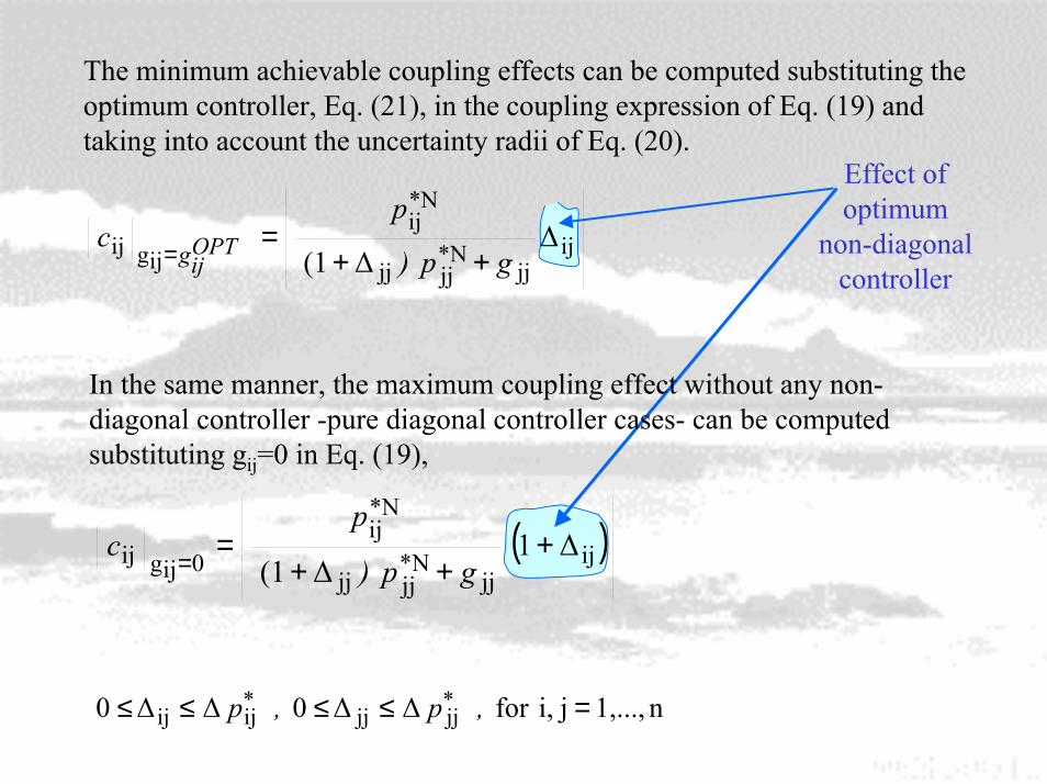
The minimum achievable coupling effects can be computed substituting theoptimum controller, Eq. (21), in the coupling expression of Eq. (19) andtaking into account the uncertainty radii of Eq. (20).
ijjj
N*jjjj
*Nij
ijgij ∆∆(1 gp)
pc OPT
ijg ++=
=
In the same manner, the maximum coupling effect without any non-diagonal controller -pure diagonal controller cases- can be computedsubstituting gij=0 in Eq. (19),
( )ijjj
N*jjjj
*Nij
0ijgij ∆1∆(1
+++
== gp)
pc
n1,...,ji,for∆∆0∆∆0 jjjjijij =≤≤≤≤ ,p,p **

16
• Consider the n x n linear multivariable system shown in Fig.1.
3.- Rejection of External Disturbances at Plant Output
Fig. 1 General structure of a MIMOsystem with plant outputand input external disturbances.
• P is the plant, P є P and P is a set of possible plants due to uncertainty,• G is the full populated matrix controller,
• Pdi and Pdo are the plant input and output disturbance transfer functions.• di’ and do’ are the plant input and output external disturbances respectively.
=
=
nnnn
n
n
nnnn
n
n
g...gg............
g...ggg...gg
G;
p...pp............
p...ppp...pp
P
21
22221
11211
21
22221
11211
r = 0 -
’ d i
P di
d i
G
u v + y
d 0
+
’ d 0
P d 0
P + +

17
• denoting the external disturbance at plant output by
• then the output due to the external disturbance at plant output is,
• and the closed loop transfer matrix TY/do that relates the disturbance atplant output to the output y becomes,
(24)
(25)
'oodo dPd =
( ) 'ododo/Yodo/Yo dPddy TTGPI ==+= −1
( ) 1−+= GPIT do/Y
r = 0 -
’ d i
P di
d i
G
u v + y
d 0
+
’ d 0
P d 0
P + +

18
• Multiplying Eq.(25) by (I + P G),• pre-multiplying by• and denoting
where Λ is the diagonal part and B the balance of P-1 respectivelyand Gd is the diagonal part and Gb the balance of G respectively
• and rearranging it, yields the next expression
TY/do = ( I + Λ-1 G )-1 + ( I + Λ-1 Gd )-1 Λ-1 [ B – (B + Gb TY/do) ]
1−P[ ]
bd
ij
GGGBPpP
+=
+Λ===− **1
(26)
[ ]
+
=+Λ===
0...p...0...
p...0
p000...000p
p*n
*n
*nn
*
1
111*ij
*1- BPP
+
=+=
0...g...0...
g...0
g000...000g
n
n
nn 1
111
bd GGG

19
the only part which has anon-diagonal structure. Itwill be call the couplingmatrix Cdo
• By inspecting Equation (26) two different terms can be found:
(26)
A diagonal termTY/do-d = ( I + Λ-1 Gd ) -1
(27) A non-diagonal termTY/do-b = ( I + Λ-1 Gd )-1 Λ-1 [ B – (B + GbTY/do)](29)
TY/do = ( I + Λ-1 Gd )-1 + ( I + Λ-1 Gd )-1 Λ-1 [ B – (B + Gb TY/do) ]
1 ≤ i ≤ n
* 1 ii p
g ii
0 y i -
u i
do i
gii *
1 ii p
u i 0 y i -
∑==
n i do c d
1 jij - do j

20
This coupling matrix is essential to analyse the reduction of the cross-coupling effects.
Cdo = B – (B + Gb TY/do)
Each element of Cdoobeys,
where is the delta of Kronecker.
The influence of the non-diagonal elements gik (i ≠ j) on the cross-couplingelements described in Eq.(32) is difficult to analyse directly because of thecomplexity of the expression.
For this reason, one hypothesis and two simplifications are stated in orderto make the quantification of coupling effects easier.
(31)
(32)
≠⇔==⇔=
=ik0δik1δ
δki
kiki
)δ(1)()δ(1 ikkjik
m
1k
*ikijij −+−−= ∑
=− tgppc *
ijdo

21
N*ijp ij∆
Note, that every uncertain plant is represented by the following family,
{ } ( ) *ijijij
N*ij
*ij ppp ∆≤∆≤∆+= 01
for i,j=1,…, n
Where is the nominal plant and thenon parametric uncertainty radii.
(20) *ijp∆
N *ijp
*ijp∆
dB
φ
N *ijp
Applying again Hypothesis H1 and Simplifications S1 and S2, the finalexpression of the coupling effect can be written as,
(33)ji;)(
)(
jj*jj
ij*ij
*jj*
ijij ≠+
+−=− gp
gpppcdo
In order to find out the optimum non-diagonal controller,• Eq. (33) is made equal to zero,• and a nominal plant that minimises the maximum non-parametric uncertainty radii in Eq. (20) is chosen,*
ijp∆
(34)N*jj
N*ij
jjoptij
p
pgg =

22
Effect ofoptimum
non-diagonalcontroller
The minimum achievable coupling effects can be computed substituting theoptimum controller, Eq. (34), in the coupling expression of Eq. (33) andtaking into account the uncertainty radii of Eq. (20).
( ) ( )jjijjj
N*jjjj
*Nij
ijgij ∆∆∆1
−++
== gp
pc OPT
ijg
In the same manner, the maximum coupling effect without any non-diagonal controller -pure diagonal controller cases- can be computedsubstituting gij=0 in Eq. (33),
n1,...,ji,for∆∆0∆∆0 jjjjijij =≤≤≤≤ ,p,p **
( ) ( )ijjj
N*jjjj
*Nij
0ij ∆1∆1
+++
== gp
pc
ijg

23
4.- Design Methodology
Composed of n stages, as many as loops, performs the following steps for everycolumn of the matrix controller G.
⇒⇒
⇒
=
nnnk2n1n
knkk2k1k
n2k22221
n1k11211
2n1n
2k1k
2221
1211
1n
1k
21
11
g...g...gg
.........
g...g...gg
.........
g...g...gg
g...g...gg
...
0...0...gg
.........
0...0...gg
.........
0...0...gg
0...0...gg
0...0...0g
.........
0...0...0g
.........
0...0...0g
0...0...0g
G
Step 1 Step 2 Step n
• Stability: It is necessary and sufficient that the plant of each successive loop is stabilised(Chait and Yaniv, 1991)
• Before starting the sequential procedure, analyse the effect of interactions in the systemand identify input-output pairings using the Relative Gain Array, (Bristol, 1966).
• Afterwards, rearrange matrix P* so that ( )-1 has the smallest phase margin frequency,( )-1 the next smallest phase margin frequency, and so on, (Houpis, Rasmussen, 1999).
*p11*p22

24
Step B:
Design the (n-1) non-diagonal elements gik (i≠k, i = 1,2,...n) of the kth
controller column, minimising the coupling cdi-ik or cdo-ik described in Eqs.(19), (33), and applying the optimum non-diagonal controller equationsEq. (21) and Eq. (34) respectively.
Step A:
Design the diagonal element of the controller gkk for the inverse of equivalentplant described in Eq.(37), using a standard QFT loop-shaping method,
[ ] [ ][ ] ( )[ ]( ) [ ] [ ]( )
[ ] ( )( )[ ]
[ ] )(
gp
gpgppp
k
kk
37 k;i 1k
11-i1-i1k*
1)-(i1)-(i
1i)1(i1k*
i1)-(i11-ii1k*
1)-(ii1k
*iik
e*ii
** PP =≥
+
++−=
=
−−
−−−−−−
25
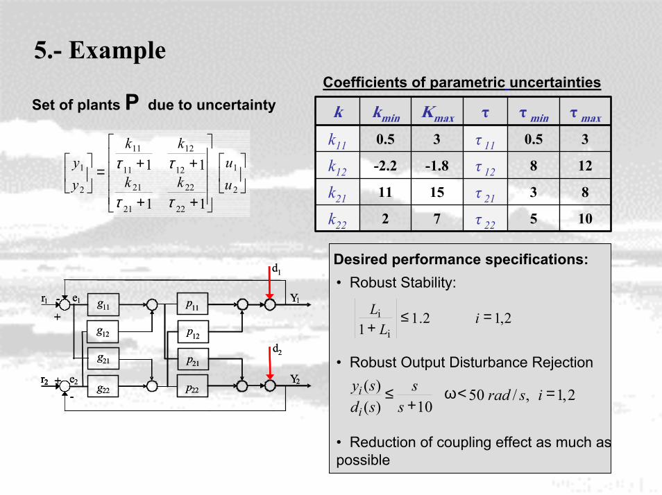
5.- Example
Set of plants P due to uncertainty
105τ 2272k22
83τ 211511k21
128τ 12-1.8-2.2k12
30.5τ 1130.5k11
τ maxτ minτKmaxkmink
++
++=
2
1
22
22
21
21
12
12
11
11
2
1
11
11uu
kk
kk
yy
ττ
ττ
Coefficients of parametric uncertainties
+
+
-
-
e1
e2
r1
r2
Y1
p12
p21
g11
g22
+
+
-
-r2 Y2
d1
d2
g12
g21
p11
p22
+
+
-
-
e1
e2
r1
r2
Y1
p12
p21
g11
g22
+
+
-
-r2 Y2
d1
d2
g12
g21
p11
p22
Desired performance specifications:• Robust Stability:
• Robust Output Disturbance Rejection
• Reduction of coupling effect as much aspossible
2,12.11 i
i =≤+
iL
L
2,1,/5010)(
)( =<ω+
≤ israds
ssdsy
i
i

26
Relative Gain Array
127325 plants generated due to uncertainty:
λ11є [0 , 0.1) for 22220 plants
λ11є [0.1 , 0.2) for 39985 plants
λ11є [0.2 , 0.3) for 35695 plants
λ11є [0.3 , 0.4) for 23155 plants
λ11є [0.4 , 0.5] for 6270 plants
0 500 1000 1500 2000 25000
0.05
0.1
0.15
0.2
0.25
0.3
0.35
0.4
0.45
0.5Value s of landa11
Numbe r of sample s
land
a11
0.005.00
10.0015.0020.0025.0030.0035.00
%
0.4-0.5
Values of landa
Values of landa. Percentage.
0.3-0.40.2-0.30.1-0.20-0.10.005.00
10.0015.0020.0025.0030.0035.00
%
0.4-0.5
Values of landa
Values of landa. Percentage.
0.3-0.40.2-0.30.1-0.20-0.1

27
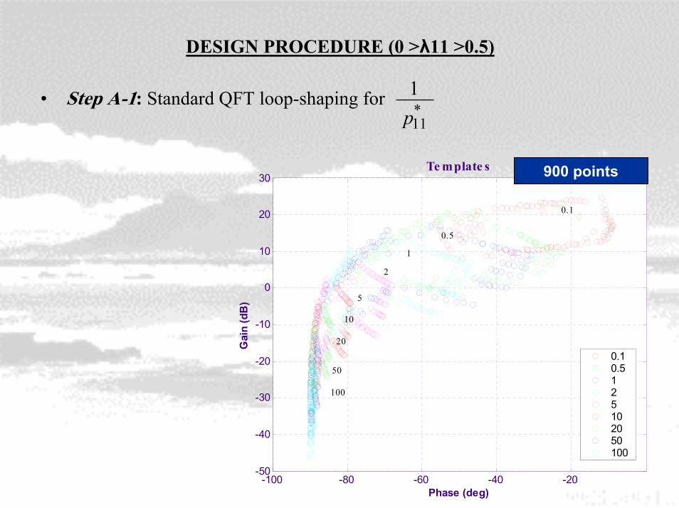
DESIGN PROCEDURE (0 >λ11 >0.5)
• Step A-1: Standard QFT loop-shaping for*11
1p
-100 -80 -60 -40 -20 0-50
-40
-30
-20
-10
0
10
20
30
0.1
0.5
1
2
5
10
20
50
100
Phase (deg)
Gai
n (d
B)
Templates
0.10.5125102050100
22770 points
28
DESIGN PROCEDURE (0 >λ11 >0.5)
• Step A-1: Standard QFT loop-shaping for*11
1p
-100 -80 -60 -40 -20-50
-40
-30
-20
-10
0
10
20
30
0.1
0.5
1
2
5
10
20
50
100
Phase (deg)
Gai
n (d
B)
Te mplate s
0.10.5125102050100
900 points
29
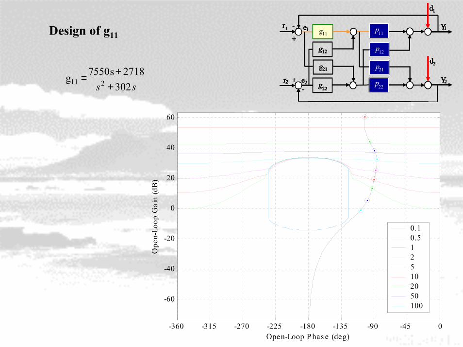
ss 3022718s7550g 211 +
+=
Design of g11
dd
+
+
- e1
e2
r1
r2
Y1
p12
p21
g11
g22r2 Y2
1
d2
g12
g21
p11
p22
e11
r2
Y1
p12
p21
g11
22-Y2
1
d2
g12
g21
p11
p22
dd
+
+
- e1
e2
r1
r2
Y1
p12
p21
g11
g22r2 Y2
1
d2
g12
g21
p11
p22
e11
r2
Y1
p12
p21
g11
22-Y2
1
d2
g12
g21
p11
p22
+
+
- e1
e2
r1
r2
Y1
p12
p21
g11
g22r2 Y2
1
d2
g12
g21
p11
p22
e11
r2
Y1
p12
p21
g11
22-Y2
1
d2
g12
g21
p11
p22
-360 -315 -270 -225 -180 -135 -90 -45 0
-60
-40
-20
0
20
40
60
Open-Loop P has e (deg)
Ope
n-Lo
op G
ain
(dB
)
0.10.5125102050100
30
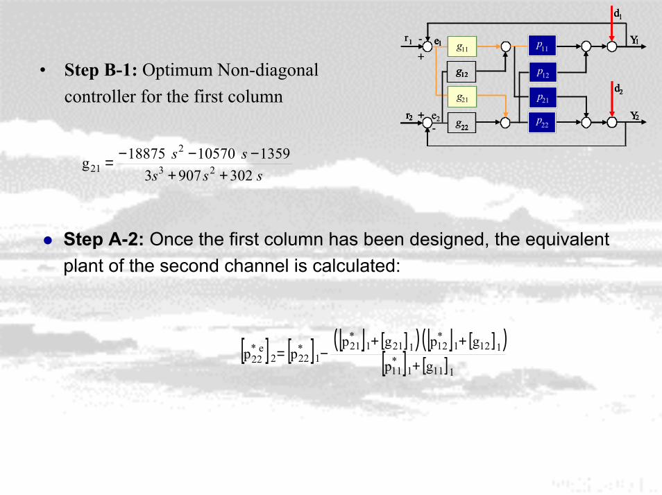
• Step B-1: Optimum Non-diagonalcontroller for the first column
sssss
302907313591057088751g 23
2
21 ++−−−=
Step A-2: Once the first column has been designed, the equivalent plant of the second channel is calculated:
[ ] [ ] [ ] [ ]( ) [ ] [ ]( )[ ] [ ]1111
*11
1121*121211
*21
1*222
e*22 gp
gpgppp
+
++−=
+
+
- e1
e2
r1
r2
Y1
p12
p21
g11
g22r2 Y2
d1
d2
g12
g21
p11
p22
e11
r2
Y1
p12
p21
g11
22-Y2
d1
d2
g12
g21
p11
p22
+
+
- e1
e2
r1
r2
Y1
p12
p21
g11
g22r2 Y2
d1
d2
g12
g21
p11
p22
e11
r2
Y1
p12
p21
g11
22-Y2
d1
d2
g12
g21
p11
p22

31
Standard QFT loop-shaping for *e22
1p
-180 -135 -90 -45 0-60
-50
-40
-30
-20
-10
0
10
20
30
0.1
0.5
1
2
5
10
20
50
100
Phas e (deg)
Gai
n (d
B)
Te mplate s
0.10.5125102050100
22842 points

32
1314 points
-180 -135 -90 -45 0-60
-50
-40
-30
-20
-10
0
10
20
30
0.1
0.5
1
2
5
10
20
50
100
Phas e (deg)
Gai
n (d
B)
Te mplate s
0.10.5125102050100
Standard QFT loop-shaping for *e22
1p
33
+
+
- e1
e2
r1
r2
Y1
p12
p21
g11
g22r2 Y2
d1
d2
g12
g21
p11
p22
e11
r2
Y1
p12
p21
g11
22-Y2
d1
d2
g12
g21
p11
p22
+
+
- e1
e2
r1
r2
Y1
p12
p21
g11
g22r2 Y2
d1
d2
g12
g21
p11
p22
e11
r2
Y1
p12
p21
g11
22-Y2
d1
d2
g12
g21
p11
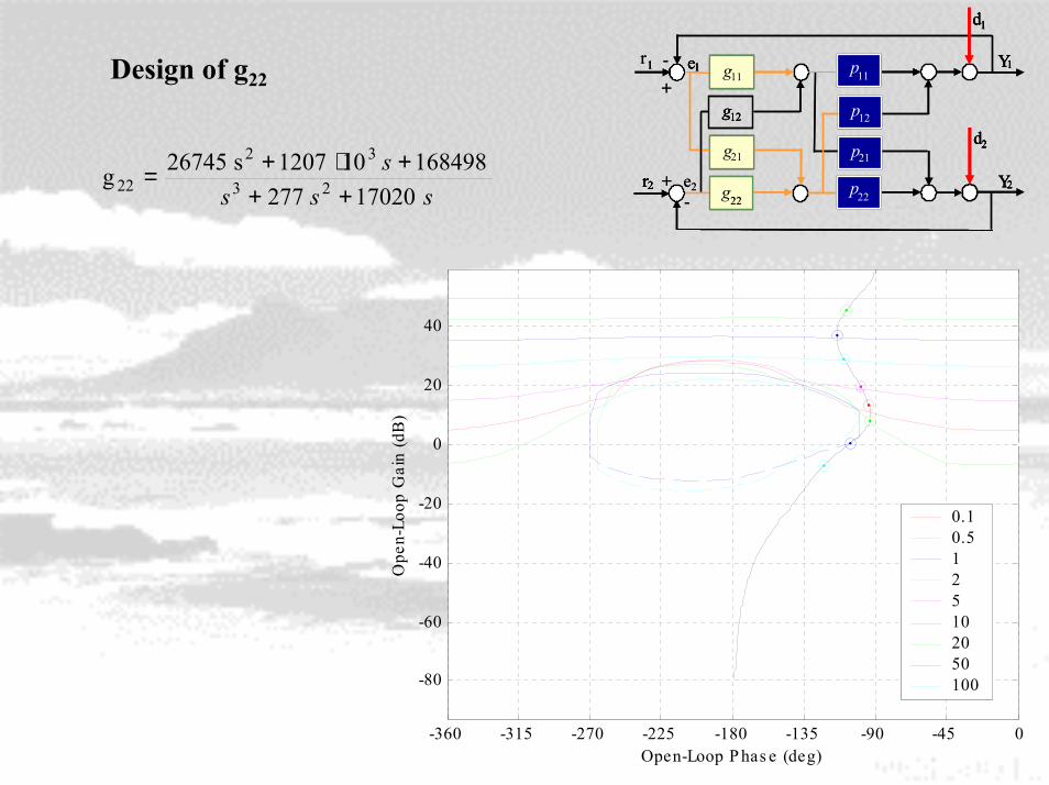
p22ssss
17020277168498101207s26745g 23
32
22 +++⋅+=
Design of g22
-360 -315 -270 -225 -180 -135 -90 -45 0
-80
-60
-40
-20
0
20
40
Open-Loop P has e (deg)
Ope
n-Lo
op G
ain
(dB
)
0.10.5125102050100

34
• Step B-2: Optimum Non-diagonal controller for the second column
sssssss14187.170471.277
18725108.1104.37430g 234
5253
12 ++++⋅+⋅+=
+
+
- e1
e2
r1
r2
Y1
p12
p21
g11
g222 Y2
d 1
d 2
g12
g21
p11
p22
e11
2
1
p12
p21
g11
22-2
d
dg12
g21
p11
p22
+
+
- e1
e2
r1
r2
Y1
p12
p21
g11
g222 Y2
d 1
d 2
g12
g21
p11
p22
e11
2
1
p12
p21
g11
22-2
d
dg12
g21
p11
p22

35
• Disturbance d1 at plant output
Response y1 Response y2
+
+
-
-
e1
e2
r1
r2
Y1
p12
p21
g11
g22
+
+
-
-r2 Y2
d1
p11
p22
+
+
-
-
e1
e2
r1
r2
Y1
p12
p21
g11
g22
+
+
-
-r2 Y2
d1
p11
p22
+
+
-
-
e1
e2
r1
r2
Y1
p12
p21
g11
g22
+
+
-
-r2 Y2
d1
p11
p22
g12
g21
+
+
-
-
e1
e2
r1
r2
Y1
p12
p21
g11
g22
+
+
-
-r2 Y2
d1
p11
p22
g12
g21
RESULTS
3 3.2 3.4 3.6 3.8 4 4.2 4.4 4.6 4.8 50.9
0.95
1
1.05
1.1
1.15
1.2
1.25
1.3
Time (se conds)
y1
DIAGONAL CONTROLLER
3 3.2 3.4 3.6 3.8 4 4.2 4.4 4.6 4.8 5
0.75
0.8
0.85
0.9
0.95
1
1.05
Time (se conds)
y2
DIAGONAL CONTROLLERDIAGONAL CONTROLLER DIAGONAL CONTROLLER

36
3 3.2 3.4 3.6 3.8 4 4.2 4.4 4.6 4.8 50.9
0.95
1
1.05
1.1
1.15
1.2
1.25
1.3
Time (se conds)
y1
NON-DIAGONAL CONTROLLER
3 3.2 3.4 3.6 3.8 4 4.2 4.4 4.6 4.8 5
0.75
0.8
0.85
0.9
0.95
1
1.05
Time (se conds)
y2
NON-DIAGONAL CONTROLLERNON DIAGONAL CONTROLLER NON DIAGONAL CONTROLLER
• Disturbance d1 at plant output
Response y1 Response y2
+
+
-
-
e1
e2
r1
r2
Y1
p12
p21
g11
g22
+
+
-
-r2 Y2
d1
p11
p22
+
+
-
-
e1
e2
r1
r2
Y1
p12
p21
g11
g22
+
+
-
-r2 Y2
d1
p11
p22
+
+
-
-
e1
e2
r1
r2
Y1
p12
p21
g11
g22
+
+
-
-r2 Y2
d1
p11
p22
g12
g21
+
+
-
-
e1
e2
r1
r2
Y1
p12
p21
g11
g22
+
+
-
-r2 Y2
d1
p11
p22
g12
g21
RESULTS

37
RESULTS
• Disturbance d2 at plant output
Response y1 Response y2
+
+
-
-
e1
e2
r1
r2
Y1
p12
p21
g11
g22
+
+
-
-r2 Y2
d2
g12
g21
p11
p22
+
+
-
-
e1
e2
r1
r2
Y1
p12
p21
g11
g22
+
+
-
-r2 Y2
d2
g12
g21
p11
p22
+
+
-
-
e1
e2
r1
r2
Y1
p12
p21
g11
g22
+
+
-
-r2 Y2
d2
p11
p22
+
+
-
-
e1
e2
r1
r2
Y1
p12
p21
g11
g22
+
+
-
-r2 Y2
d2
p11
p22
3 3.2 3.4 3.6 3.8 4 4.2 4.4 4.6 4.8 5
1
1.025
1.05
1.075
1.1
Time (se conds)
y1
DIAGONAL CONTROLLER
3 3.2 3.4 3.6 3.8 4 4.2 4.4 4.6 4.8 50.9
0.95
1
1.05
1.1
1.15
1.2
1.25
1.3
Time (se conds)
y2
DIAGONAL CONTROLLERDIAGONAL CONTROLLERDIAGONAL CONTROLLER

38
RESULTS
• Disturbance d2 at plant output
Response y1 Response y2
+
+
-
-
e1
e2
r1
r2
Y1
p12
p21
g11
g22
+
+
-
-r2 Y2
d2
g12
g21
p11
p22
+
+
-
-
e1
e2
r1
r2
Y1
p12
p21
g11
g22
+
+
-
-r2 Y2
d2
g12
g21
p11
p22
+
+
-
-
e1
e2
r1
r2
Y1
p12
p21
g11
g22
+
+
-
-r2 Y2
d2
p11
p22
+
+
-
-
e1
e2
r1
r2
Y1
p12
p21
g11
g22
+
+
-
-r2 Y2
d2
p11
p22
3 3.2 3.4 3.6 3.8 4 4.2 4.4 4.6 4.8 5
1
1.025
1.05
1.075
1.1
Time (se conds)
y1
NON DIAGONAL CONTROLLER
3 3.2 3.4 3.6 3.8 4 4.2 4.4 4.6 4.8 50.9
0.95
1
1.05
1.1
1.15
1.2
1.25
1.3
Time (se conds)
y2
NON DIAGONAL CONTROLLERNON DIAGONAL CONTROLLER NON DIAGONAL CONTROLLER

39
6.- Conclusions
• A QFT methodology
to design fully populated matrix controllers
to solve the MIMO external disturbance rejection problem at both,plant input and output,
and in the presence of model plant uncertainty, was presented.
• The definition of a specific coupling matrix
allows the statement of the controller design methodology.
• An example has been also presented
to improve the understanding of the methodology.

40
7.- Current Work• Applying the new methodology to control an industrial furnace.
A 7x7 MIMO System
Power: 900 kW
Length: 37.60 m
For Wind Turbine Blades Polymerisation
4.8 m
Group 1
37.600 m
7.8 m5 m5 m5 m5 m
Group 2 Group 3 Group 4 Group 5 Group 6 Group 7
5 m
Industrial furnace for compositemanufacturing located at M.Torres
(Spain)

41
EXTERNAL DISTURBANCE REJECTION INUNCERTAIN MIMO SYSTEMSWITH QFT NON-DIAGONAL
CONTROLLERS
Authors wish to gratefully appreciate the support given by the Spanish “Ministerio de Ciencia yTecnología” (MCyT) under grants CICYT DPI’2000-0785 and DPI’2003-08580-C02-01.
M. García-Sanz1, M. Barreras1, I. Egaña1, C.H. Houpis2
€
1Automatic Control and Computer Science Department,Public University of Navarra, 31006 Pamplona, SPAIN.
2Air Force Institute of Technology, Air Force ResearchLaboratory, Wright-Patterson AFB, Ohio, U.S.A.
http://www.ayc.unavarra.es/ceg/home.htmEmail: [email protected]