introduccion a excel como herramienta

8/8/2019 Introduccion a Excel como herramienta

http://slidepdf.com/reader/full/introduccion-a-excel-como-herramienta 1/33

I.1 INTRODUCTION TO EXCELSpreadsheets, such as Excel, have ceased to be strictly business applications and professionals from many

disciplines have found uses for this simple, yet powerful approach to performing mathematicalcalculations. Engineers were quick to start using electronic spreadsheets for design calculations because

of the automatic recalculation feature. Automatic recalculation allows a designer to change a variable andquickly see how that change impacts the rest of the design. Over the years, spreadsheet programs have

become more powerful and faster, allowing even larger problems to be solved.

Excel is easy to learn, and many people can start to use Excel to perform simple calculations in minutes.After learning just a few basics, most Excel users can solve a wide range of problems quickly andefficiently. The extra power available from Excel's built-in functions, graphics capabilities, and regressionoptions can be learned as needs arise. And, if needed, Excel even provides a built-in programmingenvironment that allows you to extend the capabilities of the program to meet specific needs. In the

examples and case studies that accompany this text, all of these features will be used.

Excel Basics

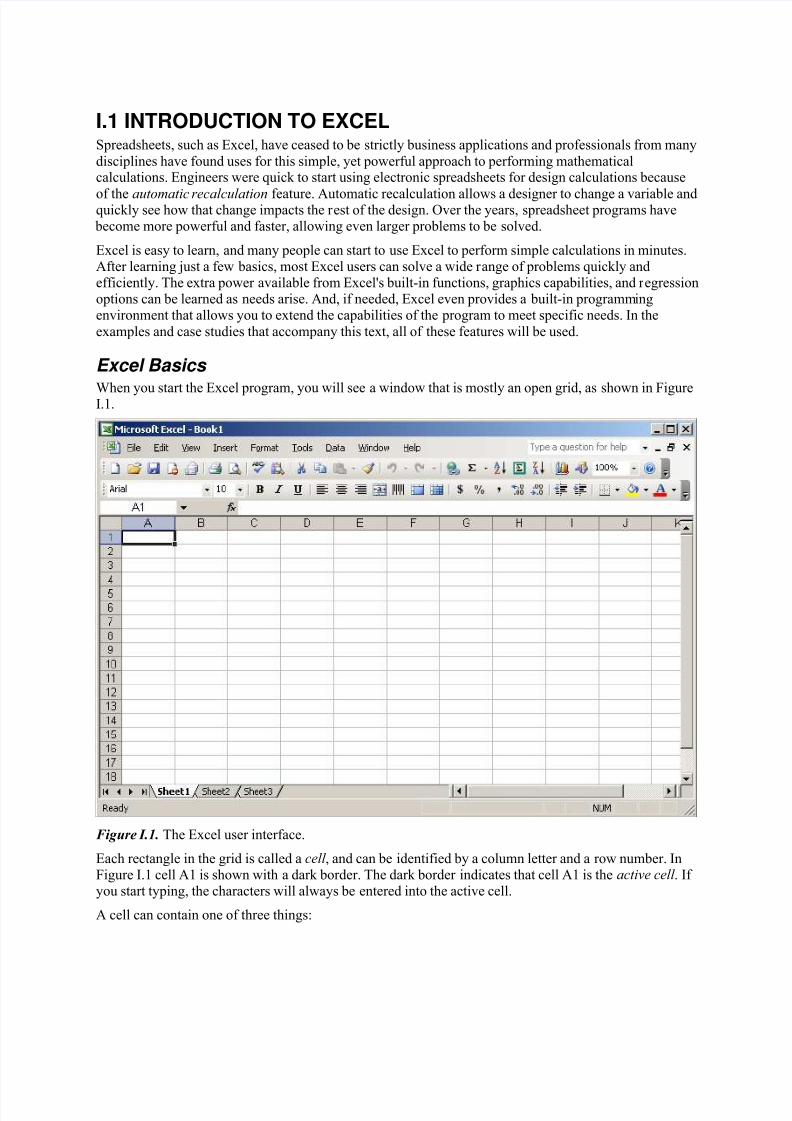
When you start the Excel program, you will see a window that is mostly an open grid, as shown in FigureI.1.

Figure I.1. The Excel user interface.

Each rectangle in the grid is called a cell , and can be identified by a column letter and a row number. InFigure I.1 cell A1 is shown with a dark border. The dark border indicates that cell A1 is the active cell . If you start typing, the characters will always be entered into the active cell.

A cell can contain one of three things:



• a number

• some text

• a formula, or equation

Excel analyzes the characters you enter into a cell to try to automatically determine which of the three you

have entered.• If you enter a numeric value (characters 0 – 9, and minus sign), Excel will recognize the number

and display the entry as a number (right justified, general format).

• If you start your cell entry with an equal sign, Excel will interpret your cell entry as an equation

(called a formula in Excel) and attempt to mathematically evaluate the formula and display theresult in the cell.

• If Excel cannot recognize your cell entry as either a number or formula, then it displays the entry

as text (left justified, general format).

When you enter a formula into a cell, the formula is stored in the cell, but the result of the calculation isdisplayed. By storing the formulas, Excel can automatically recalculate all of the equations in the

worksheet whenever any value is changed. But, by hiding the equations used to calculate the displayedvalues, it can be difficult to follow the sequence of calculations that leads to a particular result, and evenharder to find errors. In the Excel examples in this text, the equations used to calculate values are shownto the right of the displayed result. Most calculations are presented in the following format.

| variable name | displayed value | units | formulas used | note reference |

The note reference is only used when needed.

Excel allows you to enter text and formulas in any cell. Behind the scenes, Excel keeps track of whichformulas depend on which cells, so that automatic recalculation of the formulas (in the correct order) is

possible. While Excel does not care where you put the formulas, your worksheets will be much easier to

read if you present the calculations in some logical manner. In the Excel examples in this text, thecalculation order is simply from the top of the worksheet down.

Excel does not handle units, so Excel users need to be careful to watch the units in their calculations and provide conversion factors as needed. In the examples included with this text, the units of each calculatedresult are displayed to the right of the result.

The best way to learn to use Excel is to start using it. The following examples are designed to illustratesome of the features that are useful when solving design problems. While each of these examples is

available on the disk that accompanies this text, you will learn Excel faster by trying these examplesyourself.

H

D

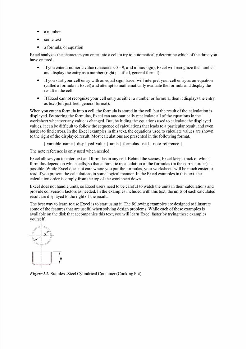
Figure I.2. Stainless Steel Cylindrical Container (Cooking Pot)



Solving Simple Models We wish to design a 1-liter capacity cooking pot, as shown in Figure I.2, to be made of 1-mm-thick stainless steel. Ultimately we would like to minimize the amount of stainless steel used. We will start withthe simplest possible model.

EXAMPLE I-1

Simple Equation-Solving Using Excel – Part A

Problem Find the height and empty weight of an open-top, cylindrical container (cooking pot)for a desired volume.

Given Volume 1 liter = 1000 cm3

Inside diameter 12 cm

Wall thickness 0.1 cm

Assumptions The material is stainless steel, mass density = 7.75 g/cm3.

Solution See Figure F-1, Tables F-1 and F-2, and Excel file Example1.xls.

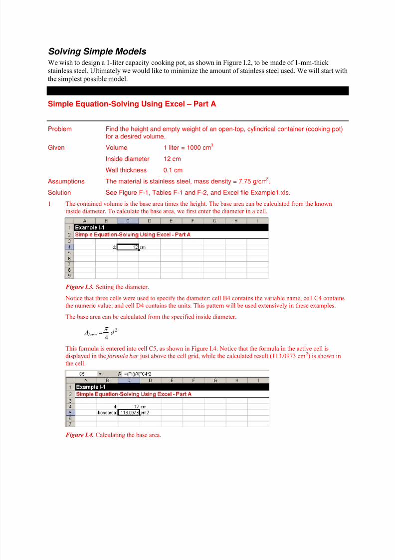
1 The contained volume is the base area times the height. The base area can be calculated from the known

inside diameter. To calculate the base area, we first enter the diameter in a cell.

Figure I.3. Setting the diameter.

Notice that three cells were used to specify the diameter: cell B4 contains the variable name, cell C4 contains

the numeric value, and cell D4 contains the units. This pattern will be used extensively in these examples.

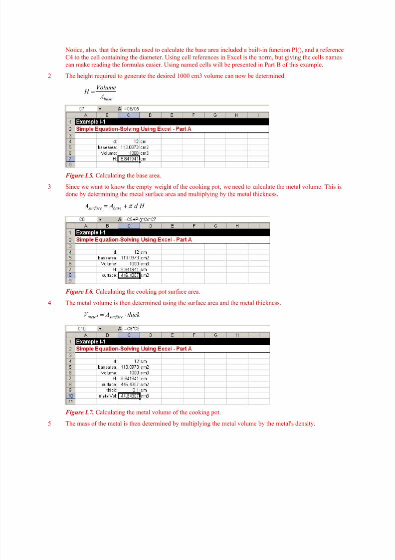
The base area can be calculated from the specified inside diameter.

2

4d Abase

π =

This formula is entered into cell C5, as shown in Figure I.4. Notice that the formula in the active cell is

displayed in the formula bar just above the cell grid, while the calculated result (113.0973 cm2) is shown in

the cell.

Figure I.4. Calculating the base area.



Notice, also, that the formula used to calculate the base area included a built-in function PI(), and a reference

C4 to the cell containing the diameter. Using cell references in Excel is the norm, but giving the cells names

can make reading the formulas easier. Using named cells will be presented in Part B of this example.

2 The height required to generate the desired 1000 cm3 volume can now be determined.

base A

Volume H =

Figure I.5. Calculating the base area.

3 Since we want to know the empty weight of the cooking pot, we need to calculate the metal volume. This is

done by determining the metal surface area and multiplying by the metal thickness.

H d A A base surface π +=

Figure I.6. Calculating the cooking pot surface area.4 The metal volume is then determined using the surface area and the metal thickness.

thick AV surfacemetal ⋅=

Figure I.7. Calculating the metal volume of the cooking pot.

5 The mass of the metal is then determined by multiplying the metal volume by the metal's density.



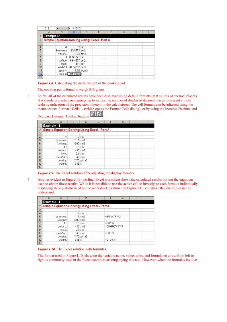
Figure I.8. Calculating the metal weight of the cooking pot.

The cooking pot is found to weigh 346 grams.

6 So far, all of the calculated results have been displayed using default formats (that is, lots of decimal places).

It is standard practice in engineering to reduce the number of displayed decimal places to present a more

realistic indication of the precision inherent in the calculations. The cell formats can be adjusted using the

menu options Format / Cells… (which opens the Format Cells dialog), or by using the Increase Decimal and

Decrease Decimal Toolbar buttons .

Figure I.9. The Excel solution after adjusting the display formats.

7 Also, as evident in Figure I.9, the final Excel worksheet shows the calculated results but not the equations

used to obtain those results. While it is possible to use the active cell to investigate each formula individually,

displaying the equations used on the worksheet, as shown in Figure I.10, can make the solution easier to

understand.

Figure I.10. The Excel solution with formulas.

The format used in Figure I.10, showing the variable name, value, units, and formula on a row from left to

right is commonly used in the Excel examples accompanying this text. However, when the formulas involve



cell addresses, they can still be hard to follow. In Part B of this example we will introduce named cells, which

can make the formulas easier to read.

Modifying Excel Worksheets to Solve Related Problems

Excel worksheets are easy to modify, which makes it possible to quickly adapt an existing solution whennecessary. In the next example, the worksheet is modified to solve for diameter instead of height.

EXAMPLE I-2

Simple Equation-Solving Using Excel – Part B

Problem Find the diameter and empty weight of an open-top, cylindrical container (cookingpot) for a desired volume.


Inside height 10 cm




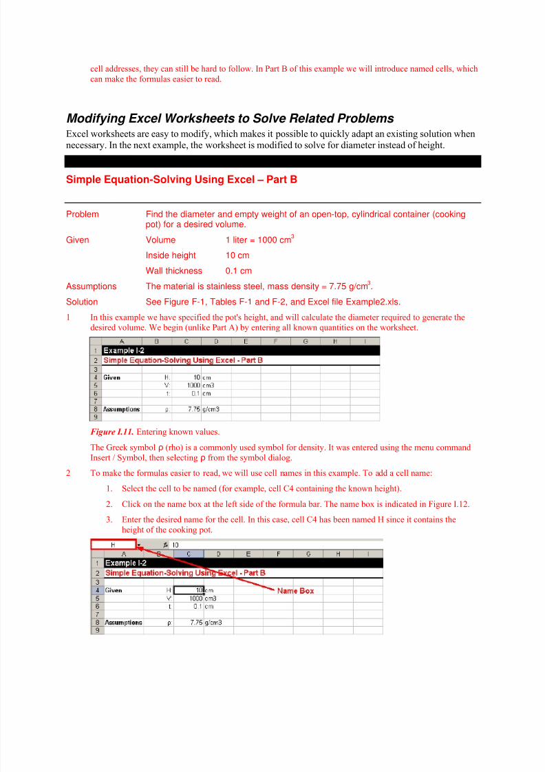
1 In this example we have specified the pot's height, and will calculate the diameter required to generate the

desired volume. We begin (unlike Part A) by entering all known quantities on the worksheet.

Figure I.11. Entering known values.

The Greek symbol ρ (rho) is a commonly used symbol for density. It was entered using the menu command

Insert / Symbol, then selecting ρ from the symbol dialog.

2 To make the formulas easier to read, we will use cell names in this example. To add a cell name:

1. Select the cell to be named (for example, cell C4 containing the known height).

2. Click on the name box at the left side of the formula bar. The name box is indicated in Figure I.12.

3. Enter the desired name for the cell. In this case, cell C4 has been named H since it contains the

height of the cooking pot.



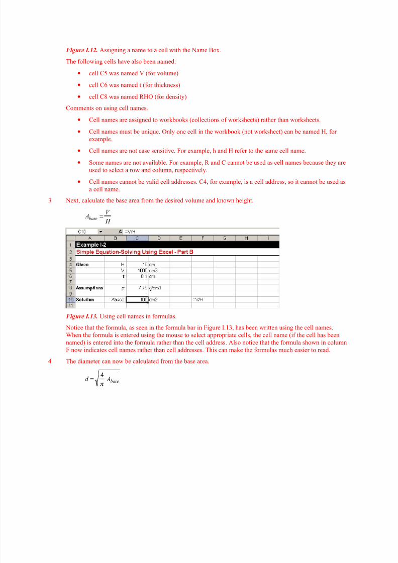
Figure I.12. Assigning a name to a cell with the Name Box.

The following cells have also been named:

• cell C5 was named V (for volume)

• cell C6 was named t (for thickness)

• cell C8 was named RHO (for density)Comments on using cell names.

• Cell names are assigned to workbooks (collections of worksheets) rather than worksheets.

• Cell names must be unique. Only one cell in the workbook (not worksheet) can be named H, for

example.

• Cell names are not case sensitive. For example, h and H refer to the same cell name.

• Some names are not available. For example, R and C cannot be used as cell names because they are

used to select a row and column, respectively.

• Cell names cannot be valid cell addresses. C4, for example, is a cell address, so it cannot be used as

a cell name.

3 Next, calculate the base area from the desired volume and known height.

H

V Abase =

Figure I.13. Using cell names in formulas.

Notice that the formula, as seen in the formula bar in Figure I.13, has been written using the cell names.

When the formula is entered using the mouse to select appropriate cells, the cell name (if the cell has been

named) is entered into the formula rather than the cell address. Also notice that the formula shown in column

F now indicates cell names rather than cell addresses. This can make the formulas much easier to read.

4 The diameter can now be calculated from the base area.

base Ad π

4=



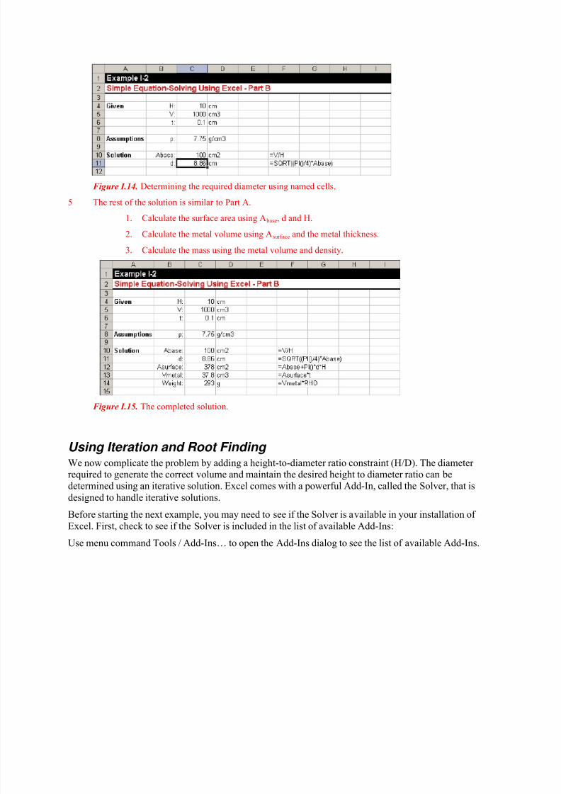
Figure I.14. Determining the required diameter using named cells.

5 The rest of the solution is similar to Part A.

1. Calculate the surface area using A base, d and H.

2. Calculate the metal volume using Asurface and the metal thickness.

3. Calculate the mass using the metal volume and density.

Figure I.15. The completed solution.

Using Iteration and Root Finding We now complicate the problem by adding a height-to-diameter ratio constraint (H/D). The diameter required to generate the correct volume and maintain the desired height to diameter ratio can bedetermined using an iterative solution. Excel comes with a powerful Add-In, called the Solver, that is

designed to handle iterative solutions.

Before starting the next example, you may need to see if the Solver is available in your installation of

Excel. First, check to see if the Solver is included in the list of available Add-Ins:

Use menu command Tools / Add-Ins… to open the Add-Ins dialog to see the list of available Add-Ins.



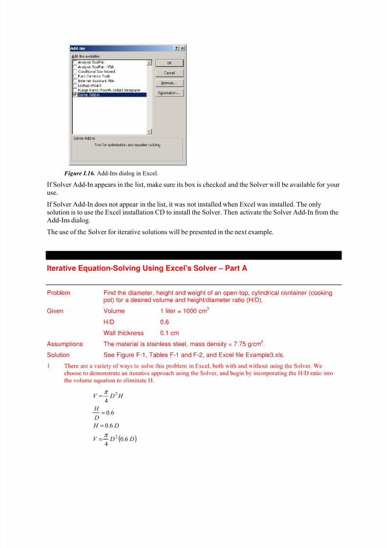
Figure I.16. Add-Ins dialog in Excel.

If Solver Add-In appears in the list, make sure its box is checked and the Solver will be available for your

use.

If Solver Add-In does not appear in the list, it was not installed when Excel was installed. The onlysolution is to use the Excel installation CD to install the Solver. Then activate the Solver Add-In from theAdd-Ins dialog.

The use of the Solver for iterative solutions will be presented in the next example.

EXAMPLE I-3

Iterative Equation-Solving Using Excel's Solver – Part A

Problem Find the diameter, height and weight of an open-top, cylindrical container (cookingpot) for a desired volume and height/diameter ratio (H/D).


H/D 0.6




1 There are a variety of ways to solve this problem in Excel, both with and without using the Solver. We

choose to demonstrate an iterative approach using the Solver, and begin by incorporating the H/D ratio into

the volume equation to eliminate H.

( ) D DV

D H

D

H

H DV

6.04

6.0

6.0

4

2

2

π

π

=

=

=

=



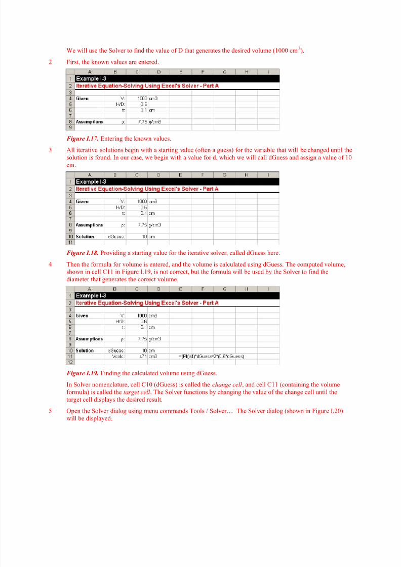
We will use the Solver to find the value of D that generates the desired volume (1000 cm3).

2 First, the known values are entered.

Figure I.17. Entering the known values.

3 All iterative solutions begin with a starting value (often a guess) for the variable that will be changed until the

solution is found. In our case, we begin with a value for d, which we will call dGuess and assign a value of 10

cm.

Figure I.18. Providing a starting value for the iterative solver, called dGuess here.

4 Then the formula for volume is entered, and the volume is calculated using dGuess. The computed volume,

shown in cell C11 in Figure I.19, is not correct, but the formula will be used by the Solver to find the

diameter that generates the correct volume.

Figure I.19. Finding the calculated volume using dGuess.

In Solver nomenclature, cell C10 (dGuess) is called the change cell , and cell C11 (containing the volume

formula) is called the target cell . The Solver functions by changing the value of the change cell until the

target cell displays the desired result.

5 Open the Solver dialog using menu commands Tools / Solver… The Solver dialog (shown in Figure I.20)

will be displayed.



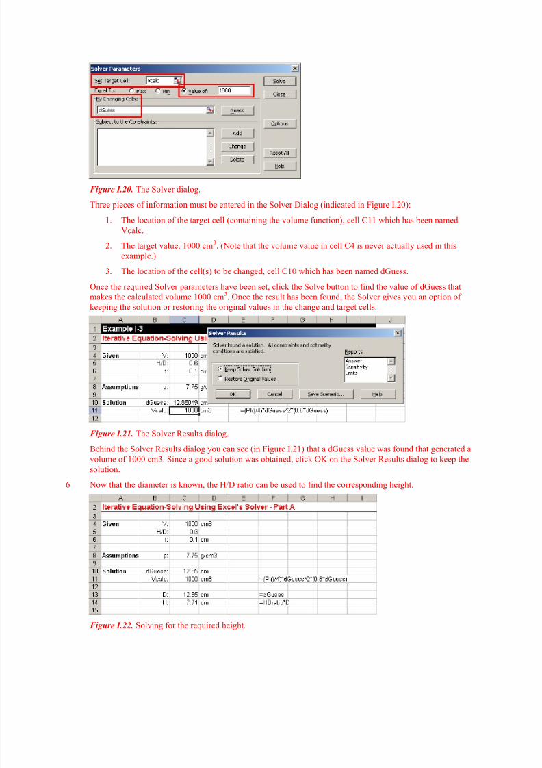
Figure I.20. The Solver dialog.

Three pieces of information must be entered in the Solver Dialog (indicated in Figure I.20):

1. The location of the target cell (containing the volume function), cell C11 which has been named

Vcalc.

2. The target value, 1000 cm3. (Note that the volume value in cell C4 is never actually used in this

example.)

3. The location of the cell(s) to be changed, cell C10 which has been named dGuess.

Once the required Solver parameters have been set, click the Solve button to find the value of dGuess that

makes the calculated volume 1000 cm3. Once the result has been found, the Solver gives you an option of

keeping the solution or restoring the original values in the change and target cells.

Figure I.21. The Solver Results dialog.

Behind the Solver Results dialog you can see (in Figure I.21) that a dGuess value was found that generated a

volume of 1000 cm3. Since a good solution was obtained, click OK on the Solver Results dialog to keep the

solution.

6 Now that the diameter is known, the H/D ratio can be used to find the corresponding height.

Figure I.22. Solving for the required height.



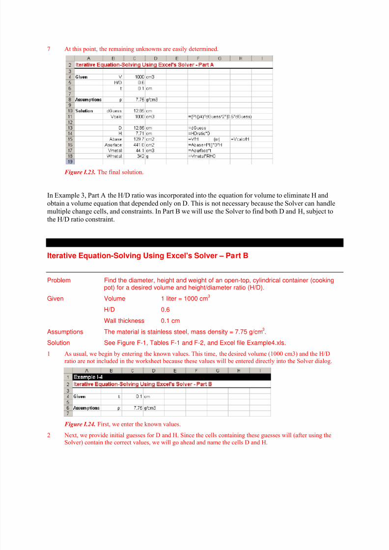
7 At this point, the remaining unknowns are easily determined.

Figure I.23. The final solution.

In Example 3, Part A the H/D ratio was incorporated into the equation for volume to eliminate H andobtain a volume equation that depended only on D. This is not necessary because the Solver can handlemultiple change cells, and constraints. In Part B we will use the Solver to find both D and H, subject tothe H/D ratio constraint.

EXAMPLE I-4

Iterative Equation-Solving Using Excel's Solver – Part B

Problem Find the diameter, height and weight of an open-top, cylindrical container (cooking

pot) for a desired volume and height/diameter ratio (H/D).Given Volume 1 liter = 1000 cm

3

H/D 0.6




1 As usual, we begin by entering the known values. This time, the desired volume (1000 cm3) and the H/D

ratio are not included in the worksheet because these values will be entered directly into the Solver dialog.

Figure I.24. First, we enter the known values.

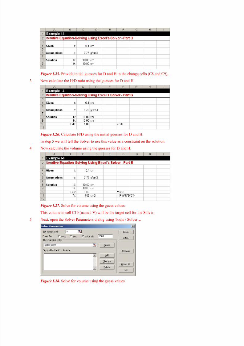
2 Next, we provide initial guesses for D and H. Since the cells containing these guesses will (after using the

Solver) contain the correct values, we will go ahead and name the cells D and H.



Figure I.25. Provide initial guesses for D and H in the change cells (C8 and C9).

3 Now calculate the H/D ratio using the guesses for D and H.

Figure I.26. Calculate H/D using the initial guesses for D and H.

In step 5 we will tell the Solver to use this value as a constraint on the solution.

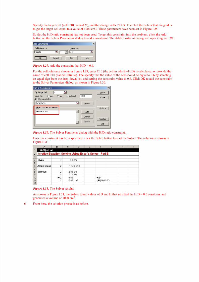
4 Now calculate the volume using the guesses for D and H.

Figure I.27. Solve for volume using the guess values.

This volume in cell C10 (named V) will be the target cell for the Solver.

5 Next, open the Solver Parameters dialog using Tools / Solver…

Figure I.28. Solve for volume using the guess values.



Specify the target cell (cell C10, named V), and the change cells C8:C9. Then tell the Solver that the goal is

to get the target cell equal to a value of 1000 cm3. These parameters have been set in Figure I.28.

So far, the H/D ratio constraint has not been used. To get this constraint into the problem, click the Add

button on the Solver Parameters dialog to add a constraint. The Add Constraint dialog will open (Figure I.29.)

Figure I.29. Add the constraint that H/D = 0.6.

For the cell reference shown in Figure I.29, enter C10 (the cell in which =H/D) is calculated, or provide the

name of cell C10 (called HDratio). The specify that the value of the cell should be equal to 0.6 by selecting

an equal sign from the drop-down list, and setting the constraint value to 0.6. Click OK to add the constraint

to the Solver Parameters dialog, as shown in Figure I.30.

Figure I.30. The Solver Parameter dialog with the H/D ratio constraint.

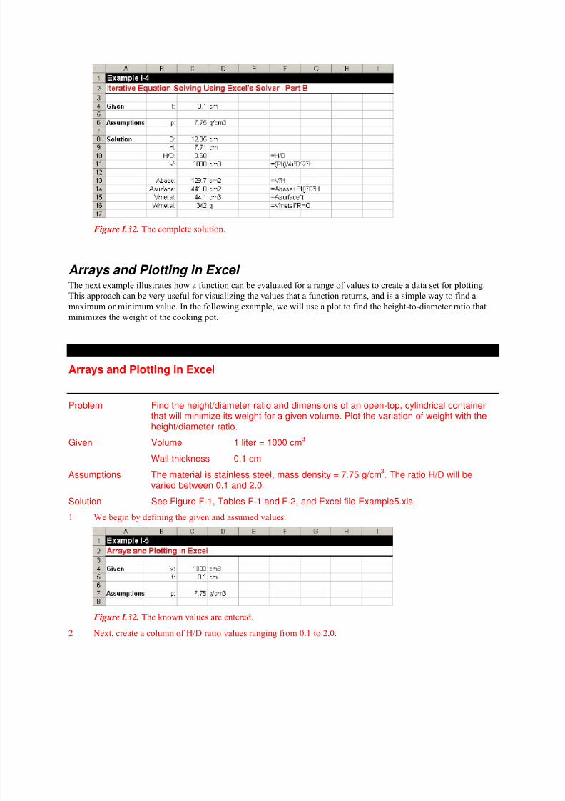
Once the constraint has been specified, click the Solve button to start the Solver. The solution is shown in

Figure I.31.

Figure I.31. The Solver results.

As shown in Figure I.31, the Solver found values of D and H that satisfied the H/D = 0.6 constraint and

generated a volume of 1000 cm3.

6 From here, the solution proceeds as before.



Figure I.32. The complete solution.

Arrays and Plotting in Excel The next example illustrates how a function can be evaluated for a range of values to create a data set for plotting.

This approach can be very useful for visualizing the values that a function returns, and is a simple way to find a

maximum or minimum value. In the following example, we will use a plot to find the height-to-diameter ratio that

minimizes the weight of the cooking pot.

EXAMPLE I-5

Arrays and Plotting in Excel

Problem Find the height/diameter ratio and dimensions of an open-top, cylindrical containerthat will minimize its weight for a given volume. Plot the variation of weight with theheight/diameter ratio.



Assumptions The material is stainless steel, mass density = 7.75 g/cm3. The ratio H/D will be

varied between 0.1 and 2.0.


1 We begin by defining the given and assumed values.

Figure I.32. The known values are entered.

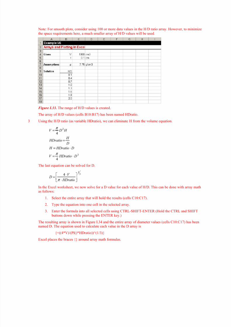
2 Next, create a column of H/D ratio values ranging from 0.1 to 2.0.



Note: For smooth plots, consider using 100 or more data values in the H/D ratio array. However, to minimize

the space requirements here, a much smaller array of H/D values will be used.

Figure I.33. The range of H/D values is created.

The array of H/D values (cells B10:B17) has been named HDratio.

3 Using the H/D ratio (as variable HDratio), we can eliminate H from the volume equation.

3

2

4

4

D HDratioV

D HDratio H

D

H HDratio

H DV

⋅=

⋅=

=

=

π

π

The last equation can be solved for D.

314

⋅

⋅=

HDratio

V D

π

In the Excel worksheet, we now solve for a D value for each value of H/D. This can be done with array math

as follows:

1. Select the entire array that will hold the results (cells C10:C17).

2. Type the equation into one cell in the selected array.

3. Enter the formula into all selected cells using CTRL-SHIFT-ENTER (Hold the CTRL and SHIFT

buttons down while pressing the ENTER key.)

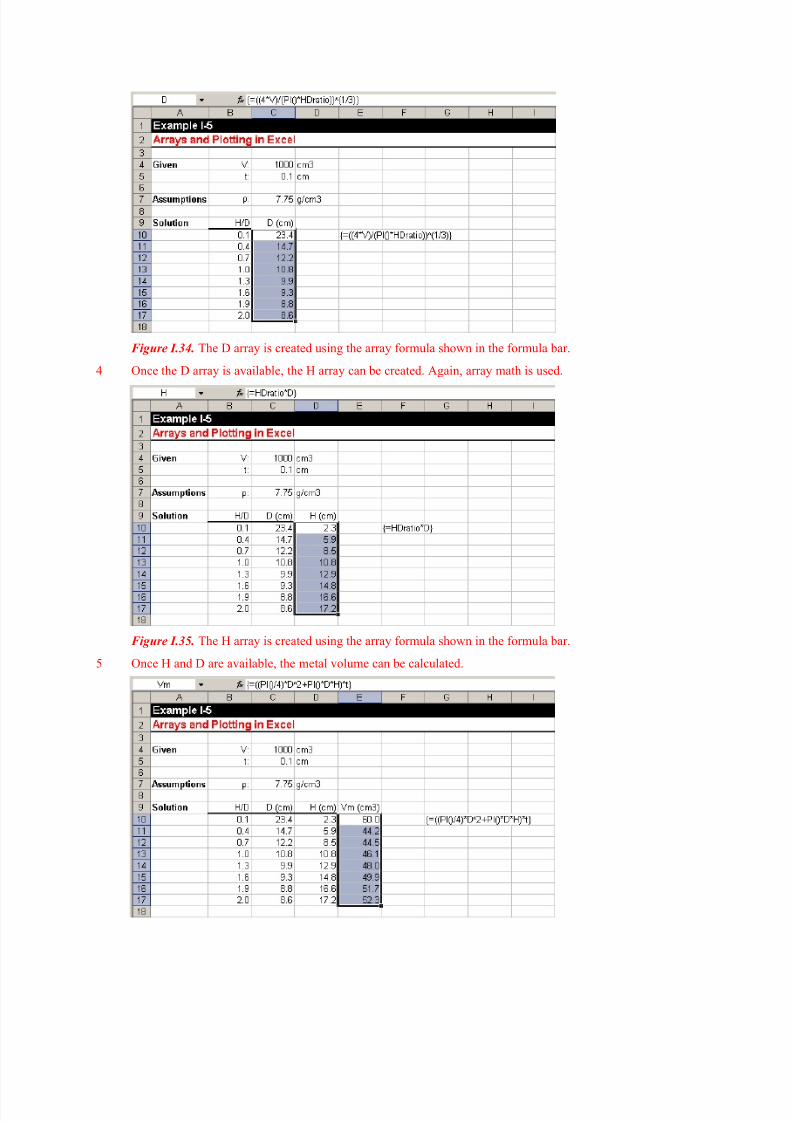
The resulting array is shown in Figure I.34 and the entire array of diameter values (cells C10:C17) has been

named D. The equation used to calculate each value in the D array is

{=((4*V)/(PI()*HDratio))^(1/3)}

Excel places the braces {} around array math formulas.



Figure I.34. The D array is created using the array formula shown in the formula bar.

4 Once the D array is available, the H array can be created. Again, array math is used.

Figure I.35. The H array is created using the array formula shown in the formula bar.

5 Once H and D are available, the metal volume can be calculated.



Figure I.36. The values in the Vm (metal volume) array are calculated using the D and H arrays.

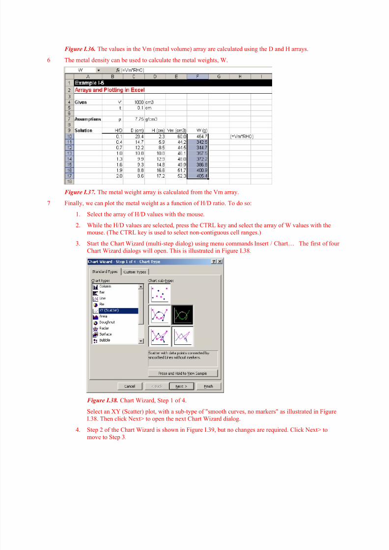
6 The metal density can be used to calculate the metal weights, W.

Figure I.37. The metal weight array is calculated from the Vm array.

7 Finally, we can plot the metal weight as a function of H/D ratio. To do so:

1. Select the array of H/D values with the mouse.

2. While the H/D values are selected, press the CTRL key and select the array of W values with the

mouse. (The CTRL key is used to select non-contiguous cell ranges.)

3. Start the Chart Wizard (multi-step dialog) using menu commands Insert / Chart… The first of four

Chart Wizard dialogs will open. This is illustrated in Figure I.38.

Figure I.38. Chart Wizard, Step 1 of 4.

Select an XY (Scatter) plot, with a sub-type of "smooth curves, no markers" as illustrated in Figure

I.38. Then click Next> to open the next Chart Wizard dialog.

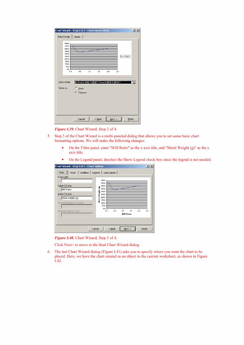
4. Step 2 of the Chart Wizard is shown in Figure I.39, but no changes are required. Click Next> to

move to Step 3.




5. Step 3 of the Chart Wizard is a multi-paneled dialog that allows you to set some basic chart

formatting options. We will make the following changes:

• On the Titles panel, enter "H/D Ratio" as the x axis title, and "Metal Weight (g)" as the y

axis title.

• On the Legend panel, deselect the Show Legend check box since the legend is not needed.


Click Next> to move to the final Chart Wizard dialog.

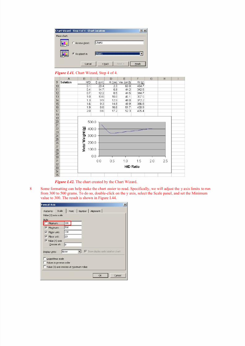
6. The last Chart Wizard dialog (Figure I.41) asks you to specify where you want the chart to be

placed. Here, we have the chart created as an object in the current worksheet, as shown in Figure

I.42.




Figure I.42. The chart created by the Chart Wizard.

8 Some formatting can help make the chart easier to read. Specifically, we will adjust the y axis limits to run

from 300 to 500 grams. To do so, double-click on the y axis, select the Scale panel, and set the Minimum

value to 300. The result is shown in Figure I.44.



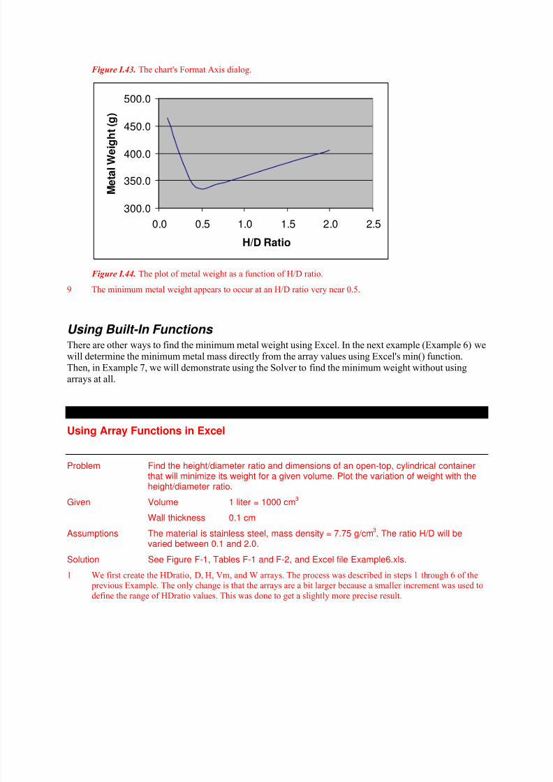
Figure I.43. The chart's Format Axis dialog.

300.0

350.0

400.0

450.0

500.0

0.0 0.5 1.0 1.5 2.0 2.5

H/D Ratio

M e t a l W e i g h

t ( g )

Figure I.44. The plot of metal weight as a function of H/D ratio.

9 The minimum metal weight appears to occur at an H/D ratio very near 0.5.

Using Built-In Functions There are other ways to find the minimum metal weight using Excel. In the next example (Example 6) wewill determine the minimum metal mass directly from the array values using Excel's min() function.Then, in Example 7, we will demonstrate using the Solver to find the minimum weight without usingarrays at all.

EXAMPLE I-6

Using Array Functions in Excel

Problem Find the height/diameter ratio and dimensions of an open-top, cylindrical containerthat will minimize its weight for a given volume. Plot the variation of weight with theheight/diameter ratio.




varied between 0.1 and 2.0.Solution See Figure F-1, Tables F-1 and F-2, and Excel file Example6.xls.

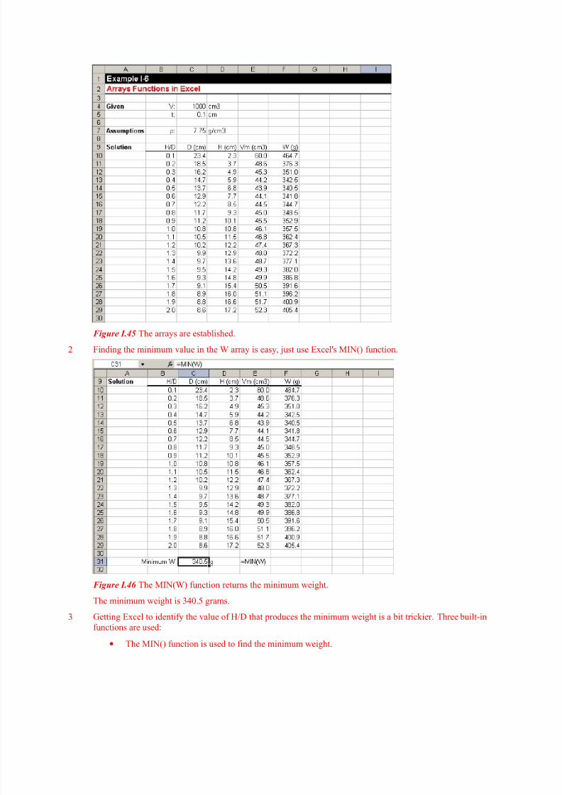
1 We first create the HDratio, D, H, Vm, and W arrays. The process was described in steps 1 through 6 of the

previous Example. The only change is that the arrays are a bit larger because a smaller increment was used to

define the range of HDratio values. This was done to get a slightly more precise result.



Figure I.45 The arrays are established.

2 Finding the minimum value in the W array is easy, just use Excel's MIN() function.

Figure I.46 The MIN(W) function returns the minimum weight.

The minimum weight is 340.5 grams.

3 Getting Excel to identify the value of H/D that produces the minimum weight is a bit trickier. Three built-in

functions are used:

• The MIN() function is used to find the minimum weight.



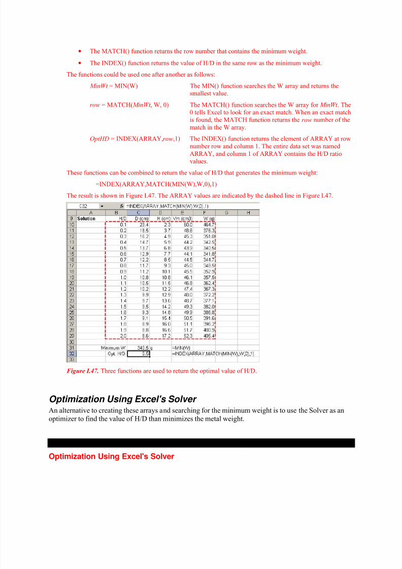
• The MATCH() function returns the row number that contains the minimum weight.

• The INDEX() function returns the value of H/D in the same row as the minimum weight.

The functions could be used one after another as follows:

MinWt = MIN(W) The MIN() function searches the W array and returns the

smallest value.

row = MATCH(MinWt , W, 0) The MATCH() function searches the W array for MinWt . The

0 tells Excel to look for an exact match. When an exact match

is found, the MATCH function returns the row number of the

match in the W array.

OptHD = INDEX(ARRAY,row,1) The INDEX() function returns the element of ARRAY at row

number row and column 1. The entire data set was named

ARRAY, and column 1 of ARRAY contains the H/D ratio

values.

These functions can be combined to return the value of H/D that generates the minimum weight:

=INDEX(ARRAY,MATCH(MIN(W),W,0),1)

The result is shown in Figure I.47. The ARRAY values are indicated by the dashed line in Figure I.47.

Figure I.47. Three functions are used to return the optimal value of H/D.

Optimization Using Excel's Solver An alternative to creating these arrays and searching for the minimum weight is to use the Solver as an

optimizer to find the value of H/D than minimizes the metal weight.

EXAMPLE I-7

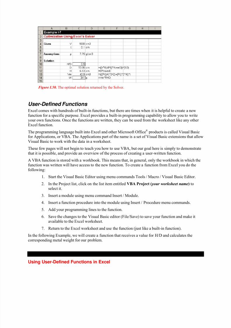
Optimization Using Excel's Solver



Problem Find the height/diameter ratio and dimensions of an open-top, cylindrical containerthat will minimize its weight for a given volume.






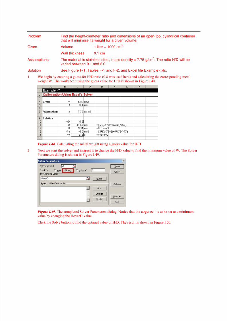
1 We begin by entering a guess for H/D ratio (0.8 was used here) and calculating the corresponding metal

weight W. The worksheet using the guess value for H/D is shown in Figure I.48.

Figure I.48. Calculating the metal weight using a guess value for H/D.

2 Next we start the solver and instruct it to change the H/D value to find the minimum value of W. The Solver

Parameters dialog is shown in Figure I.49.

Figure I.49. The completed Solver Parameters dialog. Notice that the target cell is to be set to a minimum

value by changing the HoverD value.

Click the Solve button to find the optimal value of H/D. The result is shown in Figure I.50.



Figure I.50. The optimal solution returned by the Solver.

User-Defined Functions Excel comes with hundreds of built-in functions, but there are times when it is helpful to create a new

function for a specific purpose. Excel provides a built-in programming capability to allow you to writeyour own functions. Once the functions are written, they can be used from the worksheet like any other Excel function.

The programming language built into Excel and other Microsoft Office®

products is called Visual Basicfor Applications, or VBA. The Applications part of the name is a set of Visual Basic extensions that allow

Visual Basic to work with the data in a worksheet.

These few pages will not begin to teach you how to use VBA, but our goal here is simply to demonstrate

that it is possible, and provide an overview of the process of creating a user-written function.

A VBA function is stored with a workbook. This means that, in general, only the workbook in which thefunction was written will have access to the new function. To create a function from Excel you do the

following:

1. Start the Visual Basic Editor using menu commands Tools / Macro / Visual Basic Editor.

2. In the Project list, click on the list item entitled VBA Project ( your worksheet name) toselect it.

3. Insert a module using menu command Insert / Module.

4. Insert a function procedure into the module using Insert / Procedure menu commands.

5. Add your programming lines to the function.

6. Save the changes to the Visual Basic editor (File/Save) to save your function and make itavailable to the Excel worksheet.

7. Return to the Excel worksheet and use the function (just like a built-in function).In the following Example, we will create a function that receives a value for H/D and calculates thecorresponding metal weight for our problem.

EXAMPLE I-8

Using User-Defined Functions in Excel



Problem Find the height/diameter ratio and dimensions of an open-top, cylindrical containerthat will minimize its weight for a given volume.






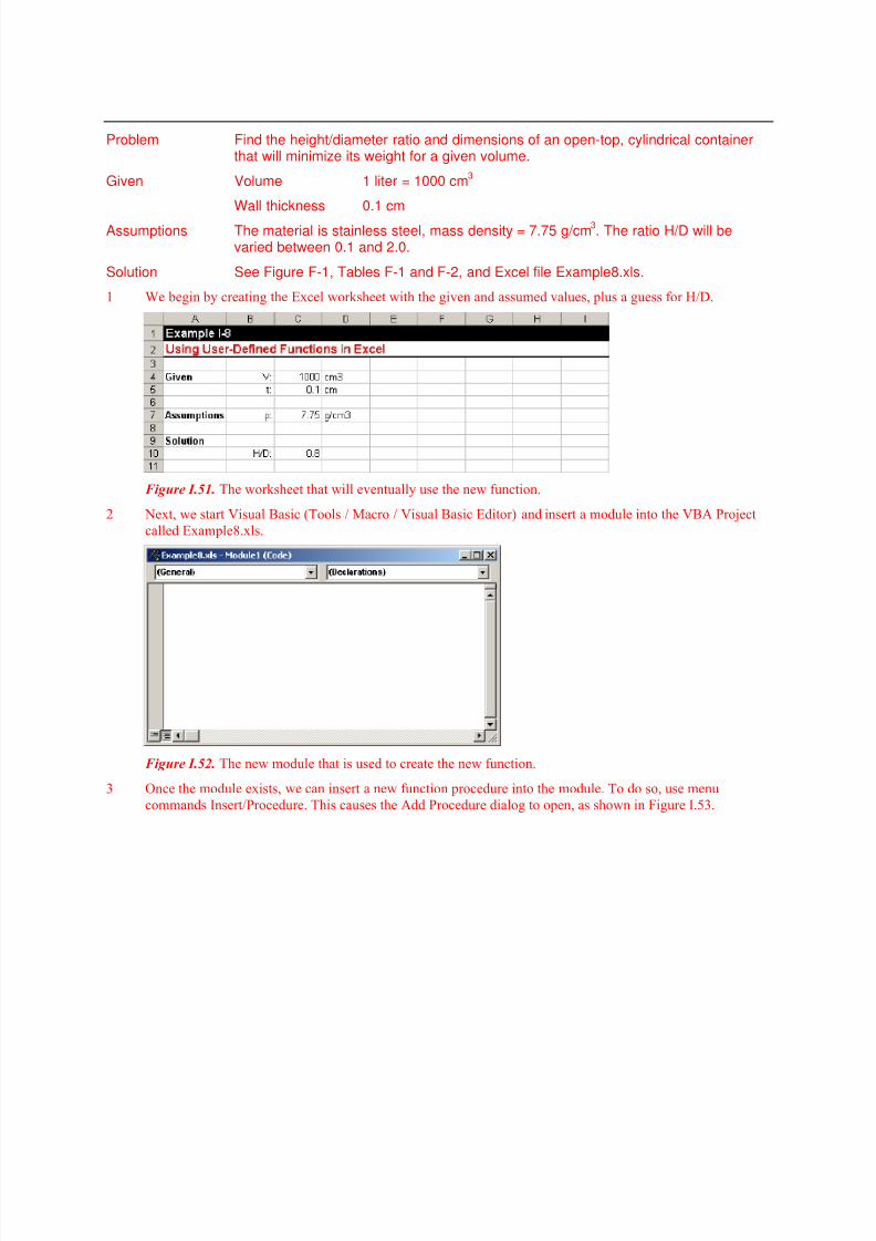
1 We begin by creating the Excel worksheet with the given and assumed values, plus a guess for H/D.

Figure I.51. The worksheet that will eventually use the new function.

2 Next, we start Visual Basic (Tools / Macro / Visual Basic Editor) and insert a module into the VBA Project

called Example8.xls.

Figure I.52. The new module that is used to create the new function.

3 Once the module exists, we can insert a new function procedure into the module. To do so, use menu

commands Insert/Procedure. This causes the Add Procedure dialog to open, as shown in Figure I.53.



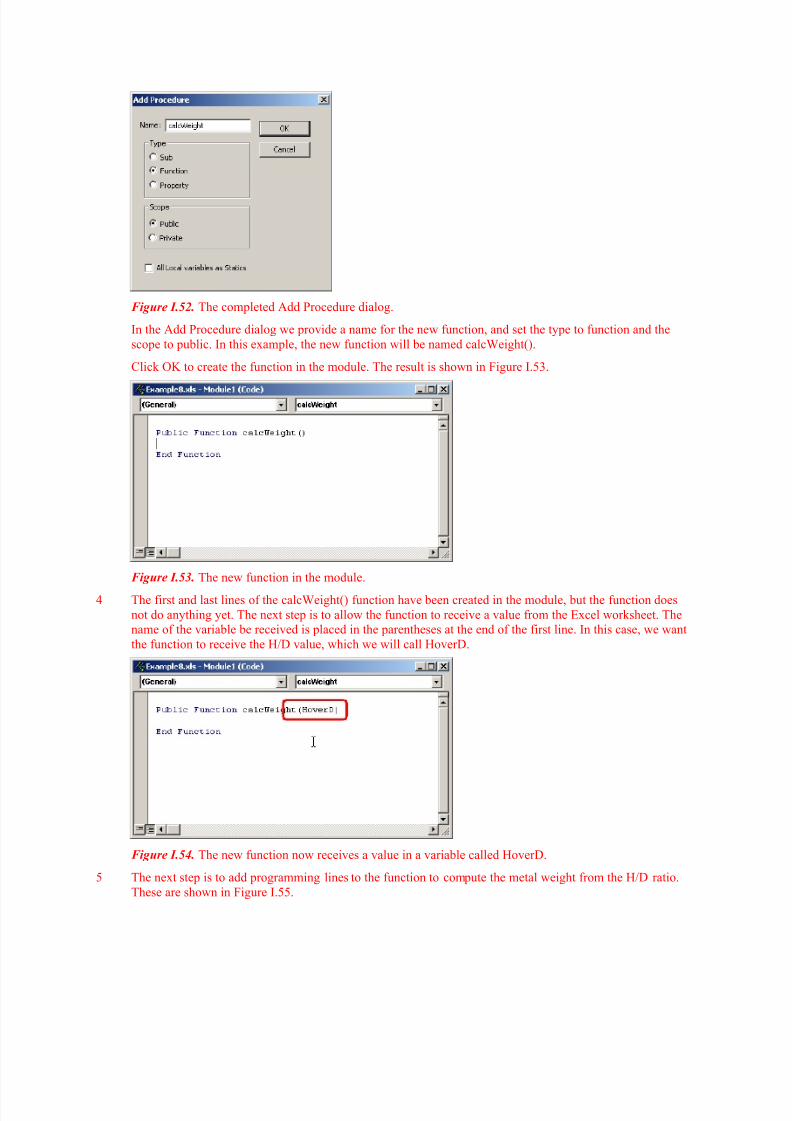
Figure I.52. The completed Add Procedure dialog.

In the Add Procedure dialog we provide a name for the new function, and set the type to function and the

scope to public. In this example, the new function will be named calcWeight().

Click OK to create the function in the module. The result is shown in Figure I.53.

Figure I.53. The new function in the module.

4 The first and last lines of the calcWeight() function have been created in the module, but the function does

not do anything yet. The next step is to allow the function to receive a value from the Excel worksheet. The

name of the variable be received is placed in the parentheses at the end of the first line. In this case, we want

the function to receive the H/D value, which we will call HoverD.

Figure I.54. The new function now receives a value in a variable called HoverD.

5 The next step is to add programming lines to the function to compute the metal weight from the H/D ratio.

These are shown in Figure I.55.



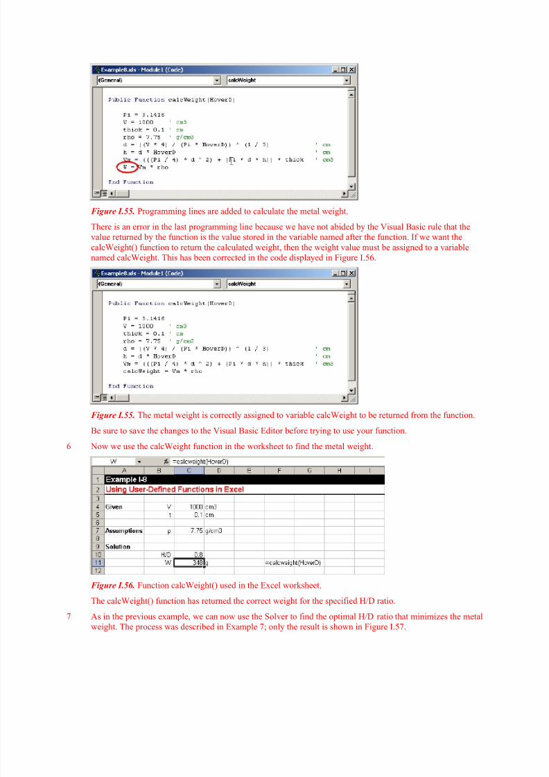
Figure I.55. Programming lines are added to calculate the metal weight.

There is an error in the last programming line because we have not abided by the Visual Basic rule that the

value returned by the function is the value stored in the variable named after the function. If we want the

calcWeight() function to return the calculated weight, then the weight value must be assigned to a variable

named calcWeight. This has been corrected in the code displayed in Figure I.56.

Figure I.55. The metal weight is correctly assigned to variable calcWeight to be returned from the function.

Be sure to save the changes to the Visual Basic Editor before trying to use your function.

6 Now we use the calcWeight function in the worksheet to find the metal weight.

Figure I.56. Function calcWeight() used in the Excel worksheet.

The calcWeight() function has returned the correct weight for the specified H/D ratio.

7 As in the previous example, we can now use the Solver to find the optimal H/D ratio that minimizes the metal

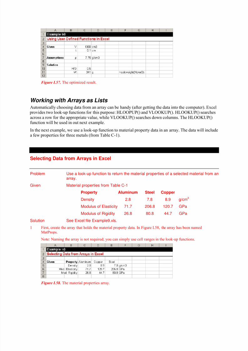
weight. The process was described in Example 7; only the result is shown in Figure I.57.



Figure I.57. The optimized result.

Working with Arrays as Lists Automatically choosing data from an array can be handy (after getting the data into the computer). Excel

provides two look-up functions for this purpose: HLOOPUP() and VLOOKUP(). HLOOKUP() searches

across a row for the appropriate value, while VLOOKUP() searches down columns. The HLOOKUP()

function will be used in out next example.

In the next example, we use a look-up function to material property data in an array. The data will includea few properties for three metals (from Table C-1).

Example I-9

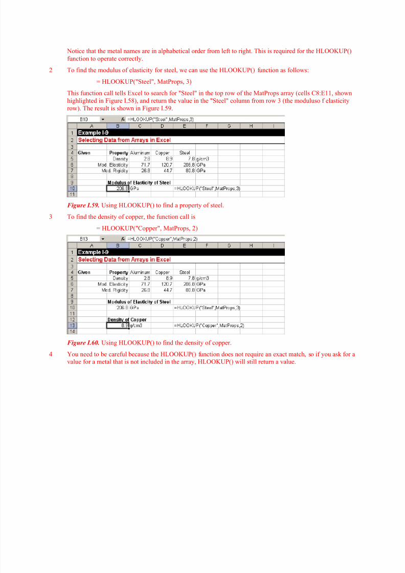
Selecting Data from Arrays in Excel

Problem Use a look-up function to return the material properties of a selected material from anarray.

Given Material properties from Table C-1

Property Aluminum Steel Copper

Density 2.8 7.8 8.9 g/cm3

Modulus of Elasticity 71.7 206.8 120.7 GPa

Modulus of Rigidity 26.8 80.8 44.7 GPa

Solution See Excel file Example9.xls.

1 First, create the array that holds the material property data. In Figure I.58, the array has been named

MatProps.

Note: Naming the array is not required; you can simply use cell ranges in the look-up functions.

Figure I.58. The material properties array.



Notice that the metal names are in alphabetical order from left to right. This is required for the HLOOKUP()

function to operate correctly.

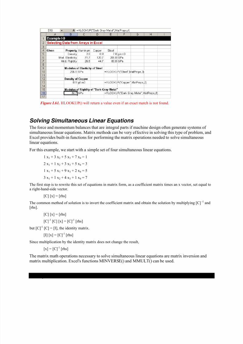
2 To find the modulus of elasticity for steel, we can use the HLOOKUP() function as follows:

= HLOOKUP("Steel", MatProps, 3)

This function call tells Excel to search for "Steel" in the top row of the MatProps array (cells C8:E11, shown

highlighted in Figure I.58), and return the value in the "Steel" column from row 3 (the moduluso f elasticityrow). The result is shown in Figure I.59.

Figure I.59. Using HLOOKUP() to find a property of steel.

3 To find the density of copper, the function call is

= HLOOKUP("Copper", MatProps, 2)

Figure I.60. Using HLOOKUP() to find the density of copper.

4 You need to be careful because the HLOOKUP() function does not require an exact match, so if you ask for a

value for a metal that is not included in the array, HLOOKUP() will still return a value.



Figure I.61. HLOOKUP() will return a value even if an exact match is not found.

Solving Simultaneous Linear Equations The force and momentum balances that are integral parts if machine design often generate systems of

simultaneous linear equations. Matrix methods can be very effective in solving this type of problem, andExcel provides built-in functions for performing the matrix operations needed to solve simultaneous

linear equations.

For this example, we start with a simple set of four simultaneous linear equations.

1 x1 + 3 x2 + 5 x3 + 7 x4 = 1

2 x1 + 1 x2 + 3 x3 + 5 x4 = 3

1 x1 + 5 x2 + 9 x3 + 2 x4 = 5

3 x1 + 1 x2 + 4 x3 + 1 x4 = 7

The first step is to rewrite this set of equations in matrix form, as a coefficient matrix times an x vector, set equal to

a right-hand-side vector.

[C] [x] = [rhs]

The common method of solution is to invert the coefficient matrix and obtain the solution by multiplying [C] -1 and

[rhs].

[C] [x] = [rhs]

[C]-1 [C] [x] = [C]-1 [rhs]

but [C]-1 [C] = [I], the identity matrix.

[I] [x] = [C]-1 [rhs]

Since multiplication by the identity matrix does not change the result,

[x] = [C]-1 [rhs]

The matrix math operations necessary to solve simultaneous linear equations are matrix inversion andmatrix multiplication. Excel's functions MINVERSE() and MMULT() can be used.

Example I-10



Solving Simultaneous Linear Equations in Excel

Problem Solve the set of four simultaneous linear equations using matrix math.

Given

1 x1 + 3 x2 + 5 x3 + 7 x4 = 1

2 x1 + 1 x2 + 3 x3 + 5 x4 = 3

1 x1 + 5 x2 + 9 x3 + 2 x4 = 5

3 x1 + 1 x2 + 4 x3 + 1 x4 = 7

Solution See Excel file Example10.xls.

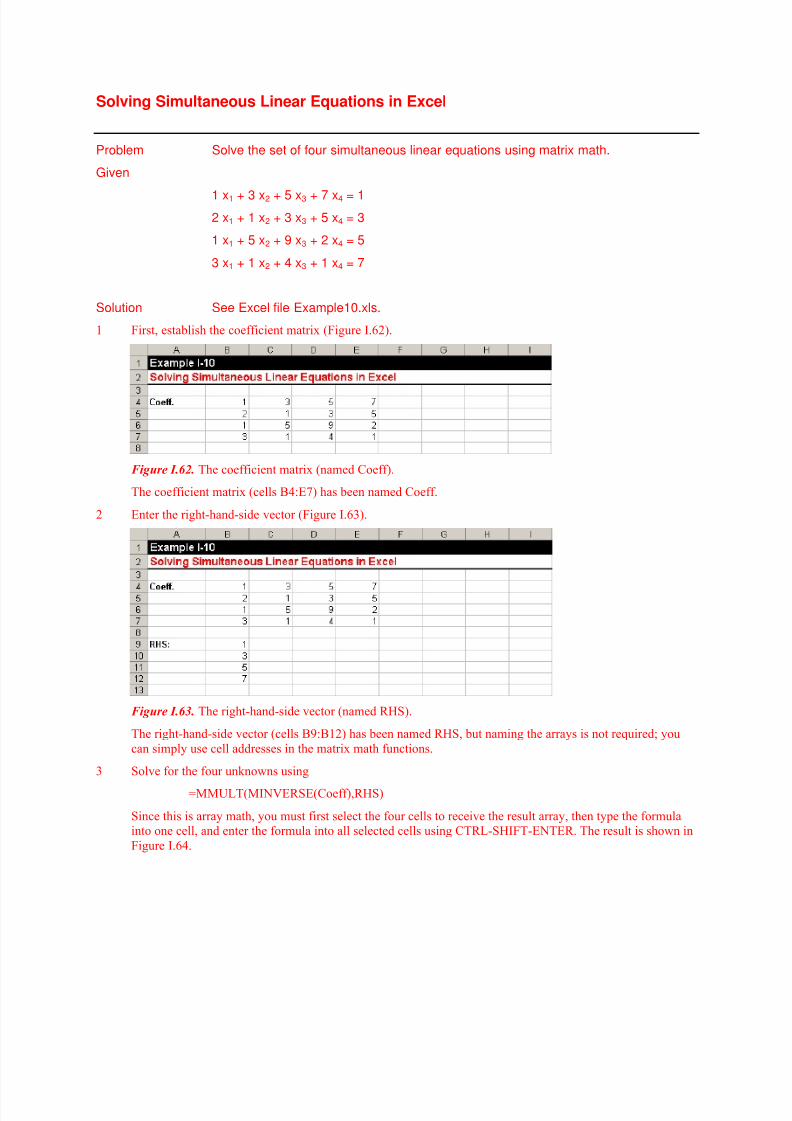
1 First, establish the coefficient matrix (Figure I.62).

Figure I.62. The coefficient matrix (named Coeff).

The coefficient matrix (cells B4:E7) has been named Coeff.

2 Enter the right-hand-side vector (Figure I.63).

Figure I.63. The right-hand-side vector (named RHS).

The right-hand-side vector (cells B9:B12) has been named RHS, but naming the arrays is not required; you

can simply use cell addresses in the matrix math functions.

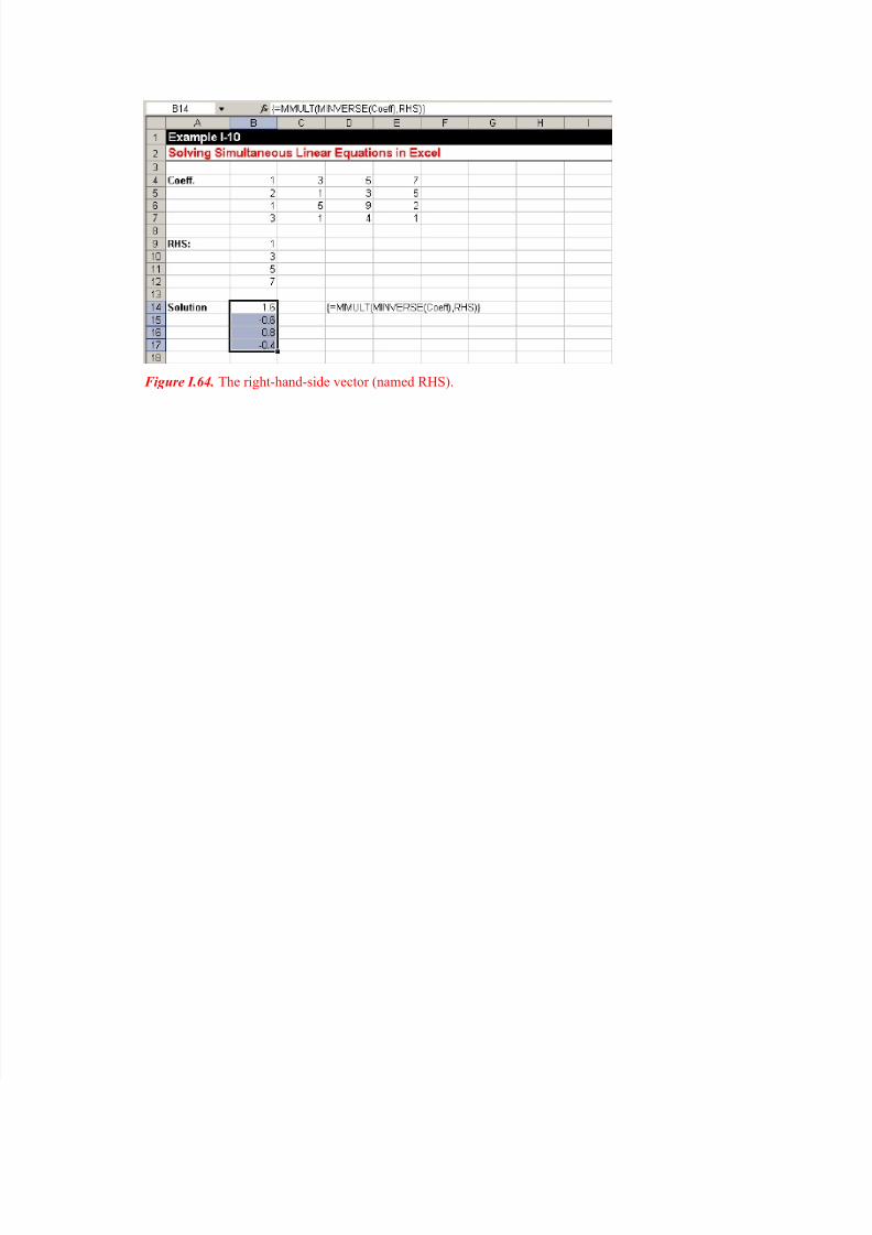
3 Solve for the four unknowns using

=MMULT(MINVERSE(Coeff),RHS)

Since this is array math, you must first select the four cells to receive the result array, then type the formula

into one cell, and enter the formula into all selected cells using CTRL-SHIFT-ENTER. The result is shown in

Figure I.64.



Figure I.64. The right-hand-side vector (named RHS).

introduccion a excel como herramienta

Documents