UNIVERSIDAD POLITÉCNICA DE MADRID

ESCUELA TÉCNICA SUPERIOR

DE INGENIEROS DE TELECOMUNICACIÓN

ESPECTROSCOPÍA ULTRASÓNICA RESONANTE SIN CONTACTO Y SU

APLICACIÓN AL ESTUDIO DE TEJIDOS VEGETALES EN ESTRUCTURA MULTICAPA

TESIS DOCTORAL

Lola Fernández-Caballero Fariñas

Máster en Ingeniería Biomédica

2016

Departamento de Tecnología Fotónica y Bioingeniería

Escuela Técnica Superior de Ingenieros de Telecomunicación

Universidad Politécnica de Madrid

Tesis Doctoral

Espectroscopía Ultrasónica Resonante Sin Contacto y su Aplicación al Estudio de Tejidos Vegetales en Estructura Multicapa

Ph.D. Thesis

Non-Contact Resonant Ultrasound Spectroscopy and its Application to Study Multilayered Vegetal Tissues

Autor

María Dolores Fernández-Caballero Fariñas Máster en Ingeniería Biomédica

Director

Tomás E. Gómez Álvarez-Arenas Doctor en Ciencias Físicas

Año

2016

Tribunal

Maurizio Mencuccini (presidente) U. of Edinburgh / U. A. de Barcelona

José Javier Serrano Olmedo (secretario) Universidad Politécnica de Madrid

Richard O’leary (vocal) University of Strathclyde

José Vicente García Pérez (vocal) Universitat Politècnica de València

Margarita González Hernández (vocal) Consejo Superior de Investigaciones Científicas

Milagros Ramos Gómez (suplente) Universidad Politécnica de Madrid

Jorge Camacho Sosa Dias (suplente) Consejo Superior de Investigaciones Científicas

Revisores Internacionales

Sergio Sanabria (Suiza) ETH, Swiss Federal Institute of Technology

Jose Brizuela (Argentina) C. N. de Investigaciones Científicas y Técnicas

"Eighty percent of success is showing up."

Woody Allen

On Language; The Elision Fields. The New York Times. August 13, 1989.

Agradecimientos

Tiene gracia que lo último que vaya a escribir de esta tesis sean los agradecimientos. Y es que, me cuesta ponerme a hacerlo. Si estáis leyendo estas líneas es porque una copia habrá llegado a vuestras manos, y si eso es así, espero no haber entrado en el selecto grupo de gente que habiendo defendido la tesis, han conseguido suspender. Entonces, suponiendo que ya sea doctora, me pongo a agradecer como es debido.

Es verdad que aquí están resumidos gran parte de los conocimientos científicos y técnicos que he adquirido en estos últimos años. Pero lo que también es cierto, es que es una pena que aquí no quede reflejado todo lo que he aprendido. Cuando me preguntan por la utilidad de una tesis doctoral y percibo cierto tono de escepticismo, suelo contestar que no sirve para mucho -en un ejercicio de hipocresía tal, que se me puede reprochar justamente-. Esta hipocresía oculta en realidad mi incapacidad para separar la utilidad mercantilista, por la que creo que me preguntan, de la utilidad personal que ha supuesto para mí realizar este trabajo y que, sin duda, eclipsa del todo a la anterior. La persona que soy hoy en día es muy diferente a la que era hace cuatro años y, desde toda la objetividad del que habla de sí mismo, creo que he mejorado. El número y riqueza de las experiencias que me ha brindado la realización de esta tesis es tal, que a menudo me he sentido culpable por tener tanta suerte. Pero, como dice mi mentor, la vida es en ocasiones ya bastante injusta como para lamentarte también cuando tienes suerte. Y es que, yo soy mucho de quejarme. Y de repetir las cosas (no sé de quién habré aprendido esto –mamá-). Dicho esto, me gustaría agradecer en primer lugar, a los que han invertido más en mí y no sólo económicamente: a mis padres, que supieron inculcarme la importancia del respeto, la humildad y la educación, así como me ayudaron a entender que ser artista -teniendo en cuenta mi falta de preparación en tales disciplinas- era un poquito arriesgado cuando acabé el instituto. En segundo lugar, a mi hermano (y a Itziar, a la que también he recurrido en repetidas ocasiones), que siempre ha sido el más inteligente de la familia, el más ultra-fondista, el que mejores regalos hace y sobretodo, el menos pesado. En tercer lugar a Tomás, si no hubiera sido él el encargado de guiarme por este camino, no creo que hubiese llegado al final (claro que igual ahora mismo, protagonizaría mi propio espectáculo en Broadway). En cuarto lugar, a todos los que ya estaban ahí antes de que comenzara esta tesis y a todos aquellos que aparecieron por y durante ella; gracias por atender mis preocupaciones -muy especialmente por escuchar aquellas que sólo tenían sentido en mi cabeza de persona que está siempre preocupada por algo- y, en definitiva, gracias por aportar a mi vida. Por último, gracias a todos los que de un modo directo o indirecto, han “patrocinado” la realización de esta tesis doctoral: la ciencia es más importante de lo que podía imaginarme antes de comenzar este camino y ahora tengo la responsabilidad moral de hacerlo entender.

Sin más, me despido esperando impaciente a que la próxima vez que tenga que escribir tantos agradecimientos sea porque esté nominada por la Academy of Motion Picture Arts and Sciences - lo mejor que tiene esto, es que no me tendrán que dar un Doctorado de estos Honoris Causa a posteriori, que yo ya iré con el mío colgando -.

Lola

“Nada me parece más acertado para definir una biografía, que esos rostros compuestos por pequeños retratos de infinidad de personajes. Las vidas se asemejan a esas páginas en blanco con puntitos que uno ha de juntar con líneas para que aparezca el dibujo. En la existencia de cada uno de nosotros, los puntos son personas que en alguna circunstancia se entrelazaron con nuestros sentimientos.”

Guillermo Fésser

Tras los pasos de Miguel de la Quadra-Salcedo. El Huffington Post. Mayo 24, 2016.

i

Prefacio

La presente memoria de tesis doctoral tiene su punto de partida en la línea de investigación iniciada en 2008 y desarrollada por la colaboración entre investigadores del Departamento de Sensores y Sistemas Ultrasónicos del Instituto de Tecnologías Físicas y de la Información del Consejo Superior de Investigaciones Científicas (ITEFI – CSIC) y de la Unidad de Recursos Forestales del Centro de Investigación y Tecnología Agroalimentaria de Aragón (CITA). Este trabajo se encuentra recogido en las publicaciones referenciadas en la descripción del estado del arte; asimismo, una parte de estos trabajos previos también se pueden consultar en la tesis del Dr. Domingo Sancho-Knapik (Sancho-Knapik 2013). Estos trabajos presentan la técnica de Espectroscopía Ultrasónica Resonante Sin Contacto (NC-RUS) como una herramienta con gran potencial para el estudio y caracterización del tejido vegetal en las hojas de plantas. Además muestran que los parámetros ultrasónicos, íntimamente ligados a la mecánica de las hojas de plantas, están también estrechamente relacionados con variables ecofisiológicas de gran interés en este campo. Sin embargo, estos trabajos anteriores se limitaban al estudio de las propiedades de la hoja en la dirección normal al plano de la misma, la consideraban como un material homogéneo e isótropo y fueron realizados siempre con hojas separadas del resto de la planta. Pese al potencial mostrado por la técnica, estas restricciones limitaban enormemente las posibilidades de la misma. La investigación desarrollada en el marco de la tesis doctoral que se presenta en esta memoria, tiene como objeto superar las limitaciones comentadas de la técnica empleando: i) modelos estratificados para considerar de manera explícita las diferentes capas de tejido presentes en la hoja, ii) direcciones de propagación diferentes a la normal, lo cual permite generar ondas de cizalla y ondas guiadas en la plano de la hoja y iii) hojas que permanecen unidas al resto de la planta mientras son medidas. Todo esto supone una mejora significativa de la técnica que permite obtener un conocimiento mucho más profundo y completo de las propiedades ultrasónicas de los tejidos vegetales y su relación con variables ecofisiológicas.

Así pues, el marco en el que se ha desarrollado esta tesis es puramente multidisciplinar, desde ámbitos como la física aplicada y caracterización de materiales hasta la biología y ecofisiología vegetal.

La introducción tratará de presentar de una manera breve los conceptos básicos necesarios para realizar una aproximación al campo de la biología. Igualmente, se contextualizará y expondrá el estado del arte de los dos ámbitos destacados implicados en esta tesis: los ultrasonidos en la caracterización de materiales y los métodos para la estimación del estado hídrico empleados en ecofisiología de plantas. En el capítulo 2, se describirán las técnicas experimentales así como los diferentes métodos teóricos utilizados. Los capítulos 3, 4, 5 y 6 recogen comunicaciones científicas realizadas durante el desarrollo de la tesis doctoral en formato de artículos científicos. Finalmente, se exponen las conclusiones generales derivadas de este trabajo además de las perspectivas futuras. Con el fin de dar una idea del trabajo del doctorando de una forma más global, se han

ii

anexado otros trabajos en los que ha colaborado y que han supuesto también parte importante en su formación.

iii

Resumen

La caracterización de materiales mediante una técnica no invasiva sin contacto, constituye un hito particularmente en aquellos casos en los que existen fuertes restricciones a este respecto: supervisión en procesos de fabricación de materiales no curados, situaciones en las que se tiene un acceso limitado a la muestra, caracterización de materiales cuyo comportamiento es sensible de ser alterado bajo contacto, etc. El perfeccionamiento de transductores ultrasónicos capaces de trabajar acoplados en aire, ha favorecido el desarrollo de técnicas como la Espectroscopía Ultrasónica Resonante Sin Contacto (NC-RUS). Dicha técnica, se empleó con éxito en la caracterización mecánica de hojas de plantas. Asimismo, se demostró que algunas de las propiedades acústicas efectivas obtenidas considerando el tejido como homogéneo, podían ser usadas como indicadores del estado hídrico de las hojas con gran precisión.

Sin embargo, el gran potencial de la técnica quedaba limitado por una serie de consideraciones no contempladas, a saber: heterogeneidad en los tejidos que componen las hojas, incidencia oblicua de la onda de ultrasonidos sobre la hoja y casos en los que la hoja no ha sido escindida del resto de la planta.

Por tanto, este trabajo se centra en la aplicación de esta técnica en situaciones no estudiadas hasta el momento como: cuantificación de las variaciones en parámetros acústicos in vivo de hojas de plantas de distintas especies sometidas a cambios en factores abióticos (como luz y agua), establecimiento de relaciones entre parámetros elásticos medidos mediante técnicas ultrasónicas y la microestructura de tejidos vegetales, extracción de parámetros mecánicos provenientes de las diferentes capas que componen materiales estratificados de uso industrial común, así como en tejidos biológicos (hojas de plantas) y generación y detección de ondas de cizalla en tejidos vegetales.

Los resultados recogidos en la realización de esta tesis doctoral indican la existencia de una variación mecánica detectable a frecuencias ultrasónicas de las hojas unidas al resto de la planta, a consecuencia de su respuesta frente a variaciones a factores tales como luz o agua. Por otro lado, valores elásticos recogidos empleando otras técnicas ultrasónicas que, además de longitudinales, excitan ondas guiadas y de cizalla en los tejidos vegetales, ponen de manifiesto la relación existente entre estos y las diferentes microestructuras que los forman. Asimismo, se han extraído parámetros mecánicos, tanto en incidencia normal como en oblicua en banda ancha ([0.1 – 1.6] MHz), relativos a las diferentes capas que forman materiales estratificados tanto del ámbito industrial como en el de las hojas de plantas.

Las conclusiones derivadas de este trabajo apuntan a la aplicación de la Espectroscopía Ultrasónica Resonante Sin Contacto como una técnica de gran potencial en la caracterización, monitorización y control de cultivos de plantas en el ámbito de la ecofisiología. Asimismo, se constata que el método desarrollado en esta tesis es de gran valor en la caracterización mecánica no sólo de materiales sintéticos, sino también en

iv

tejidos biológicos de hojas de plantas, permitiendo además, inferir parcialmente su microestructura de un modo inmediato, no destructivo y completamente no invasivo.

v

Abstract

Non-contact and non-invasive materials characterization constitutes an important milestone especially in cases where strong restrictions are mandatory, such as: monitoring of fabrication processes in uncured materials, testing samples under limited access, characterizing materials that can be altered due to contact, etc. As consequence of the advance in air-coupled ultrasonic transducers, a technique such as Non-Contact Resonant Ultrasound Spectroscopy (NC-RUS) was developed. This technique has been successfully applied in plant leaves characterization. Consequently, it was proved that effective parameters of plant leaves obtained using Non-Contact Resonant Ultrasound Spectroscopy enables an accurate estimation of plant water status.

Nevertheless, the great potential shown by this technique was limited regarding some concerns not yet studied, such as: heterogeneity in leaf tissues, oblique incidence of the ultrasonic wave in the leaves and measurements on leaves attached to the plant.

Therefore, this work is focused on the application of this technique in cases not studied so far, such as: quantifying and monitoring leaf acoustic parameters of different species while inducing changes in abiotic factors such as light and water, establishing the relationship between elastic parameters obtained by ultrasonic measurements and the microstructure of plant tissues, extracting mechanical parameters of each layer within the leaf and generating and detecting shear waves in plant tissues.

Results collected in this work show the variation in the mechanical of plant leaves attached to the plant at ultrasonic frequencies, as a consequence of their response under light and watering alterations. Furthermore, elastic values obtained using ultrasonic techniques that propagate shear and guided waves in plant tissues reveal a link between them and the microstructure observed. Additionally, acoustic parameters from different layers within the sample at ultrasonic frequencies were extracted, both at normal and oblique incidence in wideband ([0.1 – 1.6] MHz). This was demonstrated not only in plant leaves but also in synthetic materials.

From this work, we conclude that Non-Contact Resonant Ultrasound Spectroscopy (NC-RUS) technique is a powerful tool for characterization, monitoring and control of plants in the ecophysiology field. Moreover, it demonstrates that the NC-RUS technique and procedures developed in this thesis work, adds a significant value to materials characterization not only in synthetic materials but also in biological tissues such plant leaves, where it is possible to infer the microstructure in a non-destructive and non-invasive way.

vi

vii

Índice

Prefacio ............................................................................................................................. i

Resumen ......................................................................................................................... iii

Abstract ............................................................................................................................ v

Índice ............................................................................................................................. vii

Índice de Figuras ............................................................................................................ xi

CAPÍTULO 1. Introducción: Motivación y Objetivos ................................................... - 1 -

1.1. Motivación ............................................................................................................ - 3 -

1.2. Ultrasonidos y Tejido Vegetal............................................................................... - 4 -

Espectroscopía Ultrasónica Resonante Sin Contacto ............................................... - 6 -

Excitación y Detección de Resonancias Espesor .................................................. - 7 -

Modelado y Resolución del Problema Inverso para el Ajuste de Datos ............... - 8 -

1.3. Materiales Biológicos ......................................................................................... - 10 -

1.3.1. La Célula Vegetal ........................................................................................ - 10 -

El Citoesqueleto...................................................................................................... - 10 -

La Pared Celular ..................................................................................................... - 11 -

La Presión de Turgencia ........................................................................................ - 12 -

1.3.2. El Tejido Vegetal ......................................................................................... - 13 -

1.3.3. La Hoja, la Planta, y el Agua ........................................................................... - 15 -

1.4. Objetivos Generales ........................................................................................... - 18 -

CAPÍTULO 2. Métodos Teóricos y Técnicas Experimentales .................................. - 19 -

2.1. Métodos Teóricos ............................................................................................... - 21 -

2.1.1. Modelos de Propagación Ultrasónica en Hojas y Establecimiento de Resonancias ............................................................................................................... - 21 -

2.1.1.1. El Modelo de Una Capa ......................................................................... - 21 -

2.1.1.2. El Modelo Multicapa .............................................................................. - 22 -

Incidencia Oblicua .............................................................................................. - 23 -

2.1.2. El Problema Inverso: Optimización ............................................................ - 24 -

2.2. Técnicas Experimentales ................................................................................... - 27 -

2.2.1. Técnicas de Ultrasonidos ........................................................................... - 27 -

2.2.1.1. Sin Contacto ........................................................................................... - 27 -

Transmisión Directa ........................................................................................... - 28 -

Incidencia Normal (Ondas Longitudinales) ................................................... - 28 -

Incidencia Oblicua (Ondas de Cizalla) ........................................................... - 29 -

Pitch & Catch ...................................................................................................... - 29 -

Incidencia Oblicua (Ondas Guiadas) ............................................................. - 29 -

2.2.1.2. Con Contacto .......................................................................................... - 29 -

Transmisión Directa ........................................................................................... - 30 -

Incidencia Normal: Ondas Longitudinales .................................................... - 30 -

Incidencia Normal: Ondas de Cizalla ............................................................ - 30 -

Pitch & Catch ...................................................................................................... - 30 -

2.2.2. Otras Técnicas ............................................................................................ - 30 -

2.2.2.1. Medidas de Espesor y Densidad ........................................................... - 30 -

2.2.2.2. Curvas de Presión – Volumen ............................................................... - 31 -

2.2.2.3. Contenido Relativo de Agua en la Hoja ................................................ - 31 -

2.2.2.4. Conductividad Estomática ..................................................................... - 31 -

2.2.2.5. Sensores Comerciales ........................................................................... - 31 -

2.2.2.6. Imagen .................................................................................................... - 31 -

Microscopía Óptica ............................................................................................. - 31 -

Microscopía Electrónica de Barrido por Congelación ...................................... - 31 -

CAPÍTULO 3. Propagación de Ondas de Cizalla en Tejidos Vegetales mediante la técnica NC-RUS ............................................................................................................. - 33 -

CAPÍTULO 4. Aplicación de la técnica NC-RUS a Hojas de Plantas in vivo ............. - 47 -

CAPÍTULO 5. Caracterización de los Diferentes Tejidos que Constituyen las Hojas de Phormium tenax ............................................................................................................ - 69 -

CAPÍTULO 6. Extracción de Parámetros Acústicos de Materiales Multicapa Empleando NC-RUS ...................................................................................................... - 85 -

CAPÍTULO 7. Conclusiones ................................................................................... - 129 -

Conclusiones Generales ............................................................................................... - 131 -

General Conclusions ..................................................................................................... - 133 -

CAPÍTULO 8. Prospectiva ...................................................................................... - 135 -

CAPÍTULO 9. Referencias ..................................................................................... - 139 -

ANEXO I: Otras Publicaciones, Relacionadas con la Tesis, en Revistas Científicas Indexadas .............................................................................................................................. I

Ultrasonidos en Tejidos Biológicos ...................................................................................... III

NC-RUS Aplicado a Materiales No Biológicos ................................................................... XXI

ANEXO II: Otras Comunicaciones a Congresos Internacionales Relacionadas con la Tesis ...................................................................................................................................... I

Ultrasonidos en Tejidos Biológicos ...................................................................................... III

vi

Ultrasonidos en Materiales No Biológicos ........................................................................... V

vii

viii

Índice de Figuras

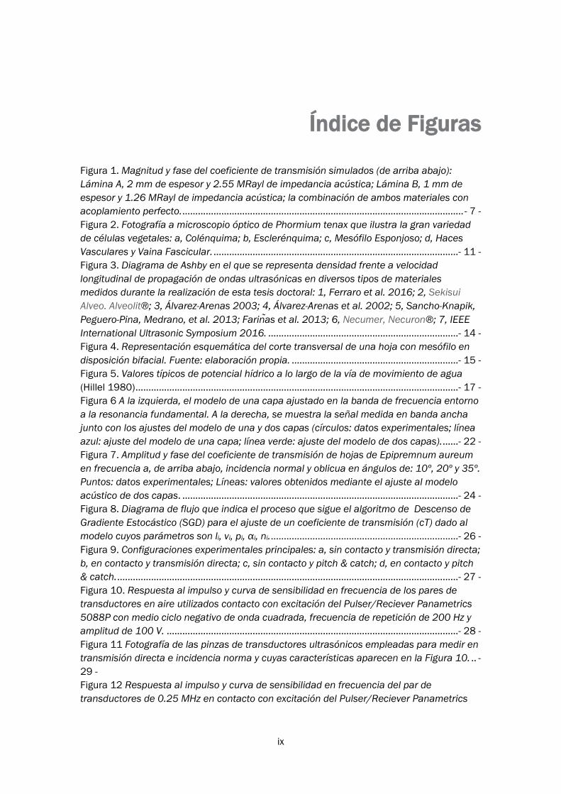
Figura 1. Magnitud y fase del coeficiente de transmisión simulados (de arriba abajo): Lámina A, 2 mm de espesor y 2.55 MRayl de impedancia acústica; Lámina B, 1 mm de espesor y 1.26 MRayl de impedancia acústica; la combinación de ambos materiales con acoplamiento perfecto. ............................................................................................................ - 7 - Figura 2. Fotografía a microscopio óptico de Phormium tenax que ilustra la gran variedad de células vegetales: a, Colénquima; b, Esclerénquima; c, Mesófilo Esponjoso; d, Haces Vasculares y Vaina Fascicular. .............................................................................................. - 11 - Figura 3. Diagrama de Ashby en el que se representa densidad frente a velocidad longitudinal de propagación de ondas ultrasónicas en diversos tipos de materiales medidos durante la realización de esta tesis doctoral: 1, Ferraro et al. 2016; 2, Sekisui Alveo. Alveolit®; 3, Álvarez-Arenas 2003; 4, Álvarez-Arenas et al. 2002; 5, Sancho-Knapik, Peguero-Pina, Medrano, et al. 2013; Farinas et al. 2013; 6, Necumer, Necuron®; 7, IEEE International Ultrasonic Symposium 2016. ......................................................................... - 14 - Figura 4. Representación esquemática del corte transversal de una hoja con mesófilo en disposición bifacial. Fuente: elaboración propia. ................................................................ - 15 - Figura 5. Valores típicos de potencial hídrico a lo largo de la vía de movimiento de agua (Hillel 1980) ............................................................................................................................ - 17 - Figura 6 A la izquierda, el modelo de una capa ajustado en la banda de frecuencia entorno a la resonancia fundamental. A la derecha, se muestra la señal medida en banda ancha junto con los ajustes del modelo de una y dos capas (círculos: datos experimentales; línea azul: ajuste del modelo de una capa; línea verde: ajuste del modelo de dos capas). ...... - 22 - Figura 7. Amplitud y fase del coeficiente de transmisión de hojas de Epipremnum aureum en frecuencia a, de arriba abajo, incidencia normal y oblicua en ángulos de: 10º, 20º y 35º. Puntos: datos experimentales; Líneas: valores obtenidos mediante el ajuste al modelo acústico de dos capas. .......................................................................................................... - 24 - Figura 8. Diagrama de flujo que indica el proceso que sigue el algoritmo de Descenso de Gradiente Estocástico (SGD) para el ajuste de un coeficiente de transmisión (cT) dado al modelo cuyos parámetros son li, vi, pi, αi, ni. ........................................................................ - 26 - Figura 9. Configuraciones experimentales principales: a, sin contacto y transmisión directa; b, en contacto y transmisión directa; c, sin contacto y pitch & catch; d, en contacto y pitch & catch. ................................................................................................................................... - 27 - Figura 10. Respuesta al impulso y curva de sensibilidad en frecuencia de los pares de transductores en aire utilizados contacto con excitación del Pulser/Reciever Panametrics 5088P con medio ciclo negativo de onda cuadrada, frecuencia de repetición de 200 Hz y amplitud de 100 V. ................................................................................................................ - 28 - Figura 11 Fotografía de las pinzas de transductores ultrasónicos empleadas para medir en transmisión directa e incidencia norma y cuyas características aparecen en la Figura 10. .. - 29 - Figura 12 Respuesta al impulso y curva de sensibilidad en frecuencia del par de transductores de 0.25 MHz en contacto con excitación del Pulser/Reciever Panametrics

ix

5077 con medio ciclo negativo de onda cuadrada centrada en 250 kHz; amplitud 100 V y recepción -19 dB. ................................................................................................................... - 30 -

x

CAPÍTULO 1

CAPÍTULO 1. Introducción: Motivación y

Objetivos

- 1 -

M.D. FARIÑAS, 2016

- 2 -

“You can't build a reputation on what you are going to do."

Henry Ford

CAPÍTULO 1

1.1. Motivación

La Espectroscopía Ultrasónica Resonante Sin Contacto (NC-RUS, por sus siglas en inglés) ha demostrado ser una técnica muy efectiva para la caracterización de materiales que, en el caso particular del estudio de hojas de plantas, nos da información relevante acerca de los tejidos que las constituyen y que, en algunos casos, puede relacionarse con medidas obtenidas mediante métodos alternativos. Estas medidas además, aportan información sobre parámetros ecofisiológicos de gran importancia, que atañen generalmente a asuntos hídricos de la planta.

La técnica que aquí se describe, presenta una serie de ventajas respecto al resto conocidas, y que se comentarán más en detalle a continuación (ver La Presión de Turgencia): como la cámara de presión, los test mecánicos clásicos, la indentación o la microscopía de fuerza atómica (AFM, por sus siglas en inglés). En primer lugar, el estudio se realiza a altas frecuencias (0.1 – 1.6 MHz) y longitud de onda considerablemente mayor que el tamaño de las células. Por ende, el campo de deformaciones producido por la onda puede considerarse homogéneo a estas escalas. Los desplazamientos causados, son de escala menor que el tamaño de las células, así que pueden entenderse en el rango lineal. Finalmente, cabe asumir que no hay cambios en el contenido de fluido de la célula pues el tiempo de relajación poroelástico es mayor que el período de la onda mecánica. Destaca, en consecuencia, el uso de esta herramienta para obtener entre otras, la contribución mecánica del agua en el tejido medido. En definitiva, la técnica de NC-RUS permite realizar medidas sobre hojas de plantas sin contacto, de forma no invasiva y no destructiva, siendo estas características que reunidas, no presenta ninguna de las técnicas estudiadas en la bibliografía.

Por tanto, esta tesis doctoral afrontará las limitaciones observadas en la NC-RUS, con el fin de desarrollar la técnica de manera que permita la monitorización sobre hojas de plantas in vivo, la obtención de parámetros acústicos diferenciados para las distintas capas de tejido y la propagación y detección de ondas en direcciones diferentes a la normal y modos no longitudinales.

- 3 -

M.D. FARIÑAS, 2016

1.2. Ultrasonidos y Tejido Vegetal

La cuantificación de propiedades mecánicas de forma no destructiva en sólidos (Agrawal et al. 2016) es fundamental para establecer valores constantes del material. En varias aplicaciones puede incluir además, la identificación de muestras y la cuantificación de la calidad de las mismas. Las acústicas han demostrado ser, dentro de estas técnicas de caracterización, una de las más fiables para extraer las propiedades fundamentales de un modo no destructivo. Los métodos de pulso-eco ultrasónicos, se han venido utilizando para determinar la velocidad del sonido en sólidos, donde un único pulso corto de alta frecuencia incide normalmente a la superficie y la onda reflejada por el sólido se analiza para estimar una velocidad de sonido, que viene dada por una distancia recorrida en un trayecto de ida y vuelta. Los métodos para estimación de la velocidad del sonido se encuentran descritos en varias revisiones en la bibliografía (Truell, Elbaum y Chick 1969). Como aspectos negativos, aunque las técnicas de pulso-eco pueden ayudar en casos en los que la muestra a inspeccionar tenga un acceso limitado, se precisa de un buen acoplamiento entre el transductor y la muestra. También pueden encontrarse limitaciones con respecto a la relación señal a ruido (SNR) debido a imprecisiones en la medida de fase, especialmente en medios dispersivos y con alta atenuación -como en el caso que tratamos: el tejido vegetal- (Levy, Agnon y Azhari 2006). En casos donde estas restricciones puedan ser limitantes, cobra sentido el uso de técnicas que comprenden excitación de modos resonantes en la muestra bajo estudio. Estos métodos que se basan en la excitación y análisis a varias frecuencias (en lugar de en una única medida de amplitud o fase) no están limitados por los mismos problemas prácticos que las medidas en pulso-eco de las que hablábamos anteriormente. La Espectroscopía Ultrasónica de Banda Ancha (Gericke 1979) se comenzó a usar como método para obtener información del tamaño y orientación de defectos en componentes metálicos a principios de los 60, cuando se desarrolló el análisis de onda reflejada sobre láminas delgadas. Posteriormente, Brekhovskikh estudió métodos teóricos para el análisis de ondas acústicas transmitidas y reflejadas en medios estratificados (Brekhovskikh 1980). Durante los 70 y 80 (Kline 1984), hubo un intenso desarrollo en los métodos digitales de procesamiento de las señales, lo cual aumentó la capacidad para medir fase y amplitud en láminas delgadas de diferentes materiales industriales. Este análisis de la señal digitalizada sería más efectivo de cara a pequeñas variaciones que el tradicional método discreto usado. En concreto, se podían medir espesores de las láminas que forman un material estratificado, incluso de aquellas a las que no se tenía acceso directo (Haines, Bell y MCIntyre 1978). Dichas medidas permitían detectar casos de daño producido por fatiga, determinar parámetros de estrés o relajación en polímeros, cambios en el curado de resinas epoxy, evaluación de adhesión de interfaces, control de degradación de materiales, monitorización de respuesta a variaciones de temperatura de materiales y determinación de tamaños y distribución de granos en materiales metálicos. Posteriormente, se introdujo el análisis en amplitud del espectro (Pialucha 1989), el cual permite obtener la velocidad de fase en el material incluso cuando las reflexiones de la onda llegan juntas en el dominio del tiempo, lo cual es muy útil en el caso de láminas delgadas. Asimismo, concluyen que la combinación de ambos métodos, fase y amplitud, dará mejores resultados. Finalmente, se aplica esta

- 4 -

CAPÍTULO 1 misma técnica utilizada en la dispersión de ondas longitudinales para el caso del análisis de ondas de cizalla (Wu 1996).

La aplicación de ultrasonidos a tejidos vegetales aparece en la bibliografía en el último medio siglo, cuando se utilizó este tejido para realizar estudios sobre los efectos biológicos de los ultrasonidos a frecuencias relevantes para uso médico (Miller 1979).

Posteriormente, se trató ya de relacionar de un modo no destructivo el contenido de agua del tejido con sus propiedades acústicas (Torii, Okamoto y Kitani 1988). Para ello, se midieron velocidades ultrasónicas, diámetro y transpiración en diferentes tipos de tallos. Se concluyó que el estado hídrico de la planta puede positivamente ser estimado de un modo cuantitativo usando una velocidad normalizada. Tras esto, Zebrowski mediría también la velocidad ultrasónica en tallo y vaina de cereales a diferentes estados de desarrollo, relacionando las adaptaciones de los cereales ante las diferentes cargas medioambientales no sólo en su morfología anatómica sino también en la heterogeneidad en los componentes de la pared celular (Żebrowski 1992).

A continuación, King y Vincent se interesaron por las propiedades mecánicas de fibras vegetales como las encontradas en hojas monocotiledóneas de Phormium tenax (King y Vincent 1996). Este interesante estudio y la sugerencia del propio J.L.F. Vincent inspirarían el trabajo incluido en el capítulo 5. Siguiendo con la aplicación de los ultrasonidos en hojas, Fukuhura determina propiedades acústicas de estas sumergidas en agua (Fukuhara 2002; Fukuhara, Okushima y Matsuo 2005). La principal limitación de este método reside en que las características determinadas sólo pueden establecerse en un estado alterado de la hoja.

Es en este contexto, en el que tiene sentido la aparición de una técnica que permitiera caracterizar tejidos vegetales de un modo no invasivo y no destructivo. Es en 2009, cuando Álvarez-Arenas publica el primer trabajo en el que se analizan medidas de espectro de magnitud y fase del coeficiente de transmisión en incidencia normal de hojas de plantas. Para ello, se excitan mediante ultrasonidos las resonancias espesor de las muestras usando transductores acoplados por aire. La resolución del problema inverso considerando la hoja como un material homogéneo permite obtener parámetros ultrasónicos de muestras de Ligustrum lucidum, Prunus laurocerasus, Populus x euroamericana y Platanus x hispánica (Álvarez-Arenas et al. 2009). En 2010, se realizaron medidas utilizando la misma técnica descrita para diferentes niveles de contenido relativo de agua en las hojas. Al mismo tiempo, se tomaron medidas de potencial hídrico empleando la cámara de presión tipo Scholander mientras que se monitorizaba el primer máximo del coeficiente de transmisión a incidencia normal en frecuencia. Se concluyó, que el punto de pérdida de turgencia de la hoja puede ser obtenido de una manera precisa empleando esta técnica ultrasónica (Sancho-Knapik et al. 2010). También, se relacionaron las variaciones en los parámetros ultrasónicos observados con los cambios estructurales que experimentaban las hojas en el proceso de deshidratación. Para ello, se tomaron imágenes de Microscopía Electrónica de Barrido por Congelación de cortes transversales de hojas de Quercus muehlenbergii. Se concluye que el parámetro c33 (módulo de elasticidad en la dirección espesor de la hoja) explica la caída en la frecuencia normalizada antes del punto de pérdida de turgencia, así como los cambios físicos en el mesófilo observados en las micrografías explican el comportamiento tras el punto de pérdida de turgencia (Sancho-Knapik et al. 2011). La técnica empleada en estos trabajos es la llamada Espectroscopía

- 5 -

M.D. FARIÑAS, 2016 Ultrasónica Resonante Sin Contacto, que se explicará con más profundidad a continuación (ver Espectroscopía Resonante Sin Contacto).

Por otro lado, también se han aplicado los ultrasonidos al estudio de tejidos vegetales en pastos. Las propiedades mecánicas de éstos son fundamentales en diversos ecosistemas. Wilson se centró en el estudio de hierbas marinas a baja frecuencia usando resonadores acústicos (Wilson y Dunton 2009). Posteriormente, también se ha estudiado la capacidad de absorción acústica de las plantas, la cual depende predominantemente de la densidad superficial de la hoja y su orientación (Horoshenkov, Khan y Benkreira 2013; Nilsson, Bengtsson y Klaeboe 2014).

Espectroscopía Ultrasónica Resonante Sin Contacto La Espectroscopía Ultrasónica Resonante (RUS) (Migliori y Darling 1996) es una técnica

que permite obtener constantes elásticas de materiales sólidos con una geometría muy definida que posibilite un análisis de las frecuencias de resonancia en sus diferentes modos de vibración (Migliori et al. 1993). Mientras que la RUS tradicional supone condiciones de contorno libres en la muestra, en el caso concreto que tratamos en este trabajo la aproximación es a través de la consideración de láminas delgadas inmersas en un medio acoplante. De esta forma aunque incrementa la complejidad en la resolución el hecho de no considerar vacío, el contrapunto lo marca la geometría de la lámina. Esta técnica acoplada por aire, es la central de esta tesis doctoral y podríamos denominarla Espectroscopía Ultrasónica Resonante Acoplada por Aire, o simplemente, Sin Contacto (NC-RUS). Cabe destacar que en este caso particular, nos enfrentamos a un problema unidimensional (dirección espesor de la lámina) y disponemos del espectro del coeficiente de transmisión del material en el aire. Dada la naturaleza del material analizado (hojas de plantas), no será posible ver más que un número limitado de resonancias excitadas a consecuencia, principalmente, de la atenuación en el tejido.

Aunque en la Espectroscopía Ultrasónica como método de ensayo no destructivo se ha venido utilizando como acoplante agua o gel acústico, paralelamente se fue sucediendo el desarrollo de transductores ultrasónicos acoplados por gas. Ciertamente, la diferencia de impedancia acústica entre cualquier medio sólido y gas es generalmente muy alta pero aun así, el uso de estos transductores se fue incorporado en el entorno industrial para aplicaciones muy concretas con altas limitaciones en la manipulación. Principalmente, se han empleado dos tipos de transductores: electrostáticos y piezoeléctricos. En el caso de estos últimos, de cara a minimizar las pérdidas por desacoplo de impedancias entre el piezoeléctrico (composite cerámico) y el aire, se emplea una conectividad 1-3 con diferentes capas de adaptación (Álvarez-Arenas et al. 2012). Con el fin de usar este tipo de transductores acoplados por aire en técnicas de espectroscopía, se precisa de un diseño que garantice un compromiso entre sensibilidad y ancho de banda de trabajo. Sin duda, el desarrollo de este tipo de transductores dentro del grupo donde se ha llevado a cabo el trabajo del doctorando, ha sido pieza clave para la implementación de la técnica que tratamos y que se ha venido usando para estudiar diversos materiales (Álvarez-Arenas 2010; Álvarez-Arenas et al. 2002; Álvarez-Arenas 2003).

La NC-RUS comprende fundamentalmente dos etapas: por un lado, la toma o simulación de medidas de coeficiente de transmisión en magnitud y fase de la muestra a caracterizar excitando resonancias espesor a frecuencias de ultrasonidos y por otro, el

- 6 -

CAPÍTULO 1 modelado de dicha muestra y la resolución del problema inverso para el ajuste del modelo a la curva de datos considerados de coeficiente de transmisión.

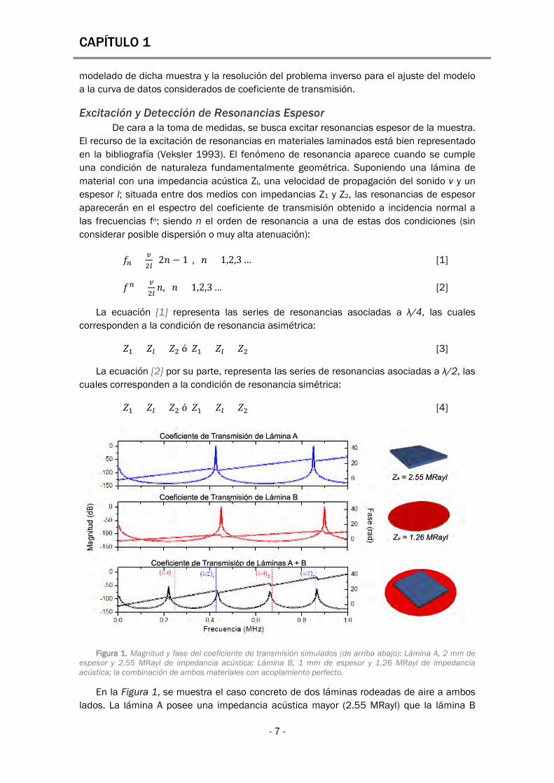
Excitación y Detección de Resonancias Espesor De cara a la toma de medidas, se busca excitar resonancias espesor de la muestra. El recurso de la excitación de resonancias en materiales laminados está bien representado en la bibliografía (Veksler 1993). El fenómeno de resonancia aparece cuando se cumple una condición de naturaleza fundamentalmente geométrica. Suponiendo una lámina de material con una impedancia acústica Zl, una velocidad de propagación del sonido v y un espesor l; situada entre dos medios con impedancias Z1 y Z2, las resonancias de espesor aparecerán en el espectro del coeficiente de transmisión obtenido a incidencia normal a las frecuencias fn; siendo n el orden de resonancia a una de estas dos condiciones (sin considerar posible dispersión o muy alta atenuación):

𝑓𝑓𝑛𝑛 = 𝑣𝑣2𝑙𝑙

(2𝑛𝑛 − 1), 𝑛𝑛 = 1,2,3 … [1]

𝑓𝑓𝑛𝑛 = 𝑣𝑣2𝑙𝑙𝑛𝑛, 𝑛𝑛 = 1,2,3 … [2]

La ecuación [1] representa las series de resonancias asociadas a λ/4, las cuales corresponden a la condición de resonancia asimétrica:

𝑍𝑍1 < 𝑍𝑍𝑙𝑙 < 𝑍𝑍2 ó 𝑍𝑍1 > 𝑍𝑍𝑙𝑙 > 𝑍𝑍2 [3]

La ecuación [2] por su parte, representa las series de resonancias asociadas a λ/2, las cuales corresponden a la condición de resonancia simétrica:

𝑍𝑍1 < 𝑍𝑍𝑙𝑙 > 𝑍𝑍2 ó 𝑍𝑍1 > 𝑍𝑍𝑙𝑙 < 𝑍𝑍2 [4]

Figura 1. Magnitud y fase del coeficiente de transmisión simulados (de arriba abajo): Lámina A, 2 mm de espesor y 2.55 MRayl de impedancia acústica; Lámina B, 1 mm de espesor y 1.26 MRayl de impedancia acústica; la combinación de ambos materiales con acoplamiento perfecto.

En la Figura 1, se muestra el caso concreto de dos láminas rodeadas de aire a ambos lados. La lámina A posee una impedancia acústica mayor (2.55 MRayl) que la lámina B

- 7 -

M.D. FARIÑAS, 2016 (1.26 MRayl). En esta situación, el coeficiente de transmisión muestra la serie de resonancias λ/2 por encontrarse en condición de resonancia simétrica. Sin embargo, cuando ambas láminas se encuentran unidas, aparecen las series de resonancias combinadas: la serie λ/2, generada por la lámina de alta impedancia; y la serie λ/4, proveniente de la lámina de baja impedancia que ahora se encuentra ante una situación de resonancia asimétrica (impedancia menor que la de la otra lámina y mayor que la del aire).

Prever la situación del patrón de resonancias de un multicapa a priori, entraña gran dificultad y requiere de cierto conocimiento de los materiales implicados. En el caso concreto tratado en esta tesis, el de las hojas de plantas, debido a unas características generales que cumplen los tipos de tejidos vegetales implicados, pueden acotarse las diferentes soluciones posibles a este problema (ver El Problema Inverso: Optimización). El orden en que los diferentes armónicos aparecen a lo largo de la frecuencia está influido por diversos factores, así como su distorsión puede incluso aparecer enmascarada por otros efectos superpuestos, generalmente relativos a la atenuación. También podría suceder que si la incidencia de la onda acústica se produce de forma oblicua a la superficie, otros modos resonantes aparezcan acoplados (ver Incidencia Oblicua). Este es el caso de las ondas de cizalla mientras que el ángulo de incidencia de la onda ultrasónica permanece por debajo del ángulo límite. Cuanto mayor es este ángulo, más energía se acopla en estas ondas de corte que, de provocar reverberación en el material, generaría un patrón de resonancias que se superpondría al patrón de resonancias espesor a consecuencia de la propagación de ondas longitudinales (ver Figura 7).

Modelado y Resolución del Problema Inverso para el Ajuste de Datos La segunda etapa que comprende la NC-RUS, está asentada en el modelado del

material a caracterizar y la posterior resolución del problema inverso. Siendo las hojas el material principal bajo estudio, era necesario un conocimiento a priori del tejido en cuestión y los conflictos a tener en cuenta a la hora de caracterizar un material biológico en contraposición a los industriales con los que se venía trabajando.

El limitado a la banda de frecuencia entorno a la primera resonancia, empleado en los trabajos anteriores a esta tesis doctoral, supone la estructura de la hoja como una lámina homogénea. Este modelo reproduce fielmente el comportamiento del material medido (ver El Modelo de Una Capa). En el punto de inicio de este trabajo, se planteó como limitación a abordar el hecho de ampliar el rango de frecuencias. En consecuencia, el estudio en banda ancha de estos materiales nos permite ver varios órdenes de resonancia en algunas especies y sujetos. Este espectro presenta comúnmente, una dispersión con respecto al patrón de resonancias esperado para una lámina homogénea. Esto es, la dispersión presente (Szabo 1995), se caracteriza por la aparición de los armónicos siguientes al de orden fundamental a frecuencias superiores a las esperadas (dispersión mayor que uno). Este efecto podría deberse a: dispersión anómala de baja frecuencia (cuando tanto velocidad como atenuación aumentan con la frecuencia, similar a la observada habitualmente en espumas blandas) o bien, a la presencia de capas acústicamente diferentes. Con este interrogante, se ahondó en el estudio de la estructura interna de la hoja con el fin de buscar la causa física que subyace a la dispersión observada (ver El Tejido Vegetal), concluyendo en la necesidad de considerar al menos dos capas de tejido acústicamente diferentes para explicar su comportamiento.

- 8 -

CAPÍTULO 1

Una vez alcanzado el modelo adecuado a seguir para el estudio del material a caracterizar con la técnica de NC-RUS, se procede a la resolución del problema inverso esto es: determinar un número finito de parámetros que definen el modelo. Estos parámetros pueden delimitar un parámetro físico directamente (densidad, velocidad de propagación, etc.) o bien, pueden especificar coeficientes u otras constantes que mantienen una relación funcional que describe un proceso físico (exponente de variación de la atenuación con la frecuencia). La resolución del problema inverso ha sido ampliamente utilizada hasta nuestros días en multitud de campos como son, entre otros, las matemáticas (Tarantola 2005), la mecánica (Deraemaeker et al. 2008), la geofísica (Dubovikl y King 2000) o la física médica (Hämäläinen et al. 1993).

El proceso de resolución del problema inverso finaliza con al ajuste del modelo a la colección de datos mediante la asignación de valores a los parámetros de este. Aunque sería posible determinar simultáneamente espesor y velocidad de una lámina medida mediante la NC-RUS (Álvarez-Arenas 2010), es preciso realizar este reajuste en los valores de los parámetros que definen nuestro modelo de cara a obtener mejores resultados. Especialmente en el caso del modelo multicapa este paso no es trivial, puesto que de su optimización depende en gran parte el éxito en la consecución de resultados satisfactorios. El algoritmo utilizado en la actualidad es el denominado Descenso de Gradiente Estocástico (SGD, por sus siglas en inglés), cuya rutina se comentará más en profundidad (ver El Problema Inverso: Optimización).

- 9 -

M.D. FARIÑAS, 2016

1.3. Materiales Biológicos

La principal particularidad que destaca en los materiales biológicos (Meyers et al. 2008), y de la cual derivan todas las demás, es que “crecen”, en contraposición a la mayoría de sintéticos, que son fabricados generalmente por un objetivo global previamente definido. Este constante crecimiento (auto-ensamblaje) en los materiales biológicos tiene un acusado efecto en su estructura altamente jerarquizada, que se mantiene en constante cambio a consecuencia de posibles alteraciones a su alrededor (diseño mecánico adaptativo y auto-reparación) lo cual, por supuesto, presenta una alta variabilidad entre sujetos a priori similares que puede dificultar el proceso de caracterización.

La naturaleza a su vez, es capaz de completar satisfactoriamente multitud de funciones que requieren un amplio rango de propiedades mecánicas usando un número muy reducido de componentes diferentes (combinando 20 aminoácidos). Además, los procesos implicados en conseguir estos requerimientos mecánicos se realizan bajo una serie de limitaciones estrictas como son, una temperatura ambiente y un entorno acuoso. Por lo tanto, esta diversidad en los materiales biológicos radica fundamentalmente en el ingenio de su diseño. En consecuencia, el diseño y composición en los materiales biológicos, van íntimamente ligados en una conexión difícilmente separable.

Todas estas premisas no han de perderse de vista a la hora de realizar el ejercicio de caracterizar materiales provenientes de la naturaleza. Conectar nano-, micro- y meso- estructura corresponde a una aproximación que requiere de un esfuerzo multidisciplinar. Sin embargo y a pesar de dicho esfuerzo, se ha demostrado que los resultados obtenidos siguiendo este camino son fructíferos en el desarrollo de nuevos materiales (Kim, Randow y Sano 2015) y arquitecturas (Mazzoleni 2013).

1.3.1. La Célula Vegetal Existen alrededor de 35 tipos de células vegetales diferentes (ver Figura 2), todas ellas

difieren en dimensiones, forma, posición y en las características de su pared. La mayoría de células miden entre 1-100 µm, su interior está en fase líquida (citoplasma) y en él se encuentra un núcleo, una red de microtúbulos, actina y filamentos intermedios (citoesqueleto), también orgánulos de diferentes tamaños y formas, así como otras proteínas. Por su parte, la membrana plasmática que recubre la célula está formada por una bicapa semipermeable de fosfolípidos reforzada por proteínas.

Sin embargo, los elementos estructurales que otorgan la forma, el tamaño y la estabilidad a la planta en su conjunto (Geitmann 2006) son: el citoesqueleto, la pared celular y la presión de turgencia (hidroesqueleto).

El Citoesqueleto Mientras que en las células animales el citoesqueleto tiene una función estructural

clave puesto que determina la forma celular, en las vegetales no es determinante debido a la existencia de la pared. No obstante, participa de los procesos asociados con la percepción de gravedad así como en la formación del huso mitótico que interviene en la división celular y en su estructura interna.

- 10 -

CAPÍTULO 1

La Pared Celular La existencia de una pared celular es la característica distintiva principal cuando se

habla de tejido vegetal en contraposición al animal. La pared, se comporta como un exoesqueleto que determina la forma celular y actúa como barrera protectora frente a agentes patógenos (Vogler et al. 2015). Se distinguen dos estrategias mecánicas principales que sigue la pared: por un lado, la habilidad para resistir tensiones permitiendo que se establezca un hidroesqueleto basado en la presión de turgencia que posibilita, además, transmitir las fuerzas recibidas. Esta capacidad reside fundamentalmente en las paredes primarias. Por otro lado, las paredes secundarias – abundantes en la esclerénquima – son también resistentes a tensión además de a compresión.

Las propiedades mecánicas de las paredes celulares están definidas por su composición bioquímica (Gibson 2012) y por las interacciones entre los polímeros que la forman. La pared celular principal es un compuesto complejo, formado por microfibrillas de celulosa embebidas en una matriz de hemicelulosa y pectina. La pared secundaria, cuando existe, es la capa adyacente a la membrana plasmática. Contiene una alta proporción de celulosa y lignina o suberina.

Figura 2. Fotografía a microscopio óptico de Phormium tenax que ilustra la gran variedad de células vegetales: a, Colénquima; b, Esclerénquima; c, Mesófilo Esponjoso; d, Haces Vasculares y Vaina Fascicular.

Aunque obedeciendo a lo comentado sobre los materiales biológicos, las propiedades mecánicas de la célula vegetal no se limitan a su individualidad, sino que también residen en la interacción con el resto que componen el tejido, modificando las propiedades de la pared celular en función de las fuerzas que interaccionan con ella. Por esta razón, aunque se requiere el conocimiento de las propiedades mecánicas de los elementos estructurales que componen la pared, el comportamiento del conjunto del tejido es esencial. Un ejemplo que ilustra esto, es el crecimiento de una típica célula vegetal: tiene una pared flexible y delgada (alrededor de 0.1-1 µm) formada por polisacáridos complejos y proteínas estructurales. Esta fina capa puede verse a microscopio electrónico. A pesar de su delgadez, ya actúa comprimiendo y dando forma al protoplasto. El crecimiento, se producirá a base de muy lentas deformaciones en las paredes (creep): las células se disponen con sus paredes firmemente pegadas unas con otras (lámina media) imposibilitando una migración celular, por lo que la morfogénesis de la planta es más bien una división celular selectiva y una dilatación localizada. Los resultados de este crecimiento pueden ser verdaderamente impresionantes: las células que recubren la superficie de las semillas de algodón pueden multiplicar por 1000 su tamaño antes de alcanzar la madurez (Cosgrove 2005). Esta expansión es en gran parte posible gracias al

- 11 -

M.D. FARIÑAS, 2016 aumento del volumen celular producido principalmente a base de almacenar agua en la vacuola. Este hecho, genera una extensión en la pared celular que estimula que nuevos polímeros se integren en ella para evitar que se vuelva más delgada y más débil.

Mucho se conoce de la composición de las paredes celulares. Asimismo, componentes como la celulosa y la pectina con interés comercial, han sido caracterizados ampliamente en la bibliografía (Edge et al. 2000; Jarvis 1984). Con todo, la caracterización mecánica de las paredes celulares en su estado natural supone aún hoy en día un reto, aunque se han venido aplicando grandes tensiones de deformación sobre células aisladas para su estudio (Cosgrove 1989) o en bloques de tejido, utilizando para ello extensómetros o máquinas tradicionales de ensayos mecánicos -. Los resultados obtenidos son de ayuda para entender mejor las propiedades mecánicas de la pared, pero al no haberse realizado en condiciones del todo similares a las reales (por ejemplo, los estreses sólo se aplican en una dimensión, cuando en la situación real son multidireccionales), resulta complicado relacionarlas de un modo directo con procesos como el crecimiento celular que tan influenciados están por estas cargas ausentes en los experimentos. Llegados a este punto, y aunque sin duda los datos obtenidos a este respecto son de gran ayuda, hay varios motivos por los cuales no existe una multitud de trabajos en la obtención de manera cuantitativa de datos mecánicos de paredes vegetales: en primer lugar, las células vegetales en el tejido están fuertemente unidas, haciendo de su separación una tarea que difícilmente puede no dañar su estructura para el posterior análisis. Por otro lado, la manipulación a esas escalas no es algo trivial. Sin embargo, el desarrollo de la micro- y nanomanipulación ha permitido que puedan realizarse ensayos sobre células aisladas (Wang, Wang y Thomas 2004) y analizar su comportamiento haciendo uso de un sencillo modelo.

Otro método que se ha usado para determinar el módulo elástico de la pared celular en células vivas es la sonda de presión de turgencia (Tomos y Leigh 1999). Se basa en la cuantificación de la pérdida de volumen celular relativa (vista a microscopio) a medida que una presión de turgencia es aplicada mediante esta sonda.

Por otro lado, las técnicas de nanoindentación (Forouzesh et al. 2013) y microscopía de fuerza atómica (AFM, por sus siglas en inglés) (Radotić et al. 2012) buscan obtener información cuantitativa de las paredes celulares. Para ello, se aplica un ciclo de carga-descarga con una duración y fuerza determinadas y se monitoriza la elasticidad y plasticidad de la respuesta en la deformación del material. Son varios los obstáculos que se presentan al llevar a cabo estas técnicas, si bien es cierto que han arrojado luz al hecho de que las paredes celulares no presentan una estructura uniforme.

El trabajo de Vanstreels sobre monitorización de cambios en tejido epidérmico vegetal vivo sometido a estreses mecánicos, supone una aproximación a la problemática de relacionar parámetros estructurales celulares y propiedades micromecánicas (Vanstreels et al. 2005).

La Presión de Turgencia El tejido vegetal se encuentra de manera natural, en un entorno acuoso. Al estado

energético en el que se halla este agua en las plantas se le denomina potencial hídrico y su definición llevada a nivel celular se puede expresar como el resultado de tres componentes principales: un potencial osmótico consecuencia de la concentración de solutos, un potencial matricial fruto de la posible interacción entre las moléculas de agua y otras

- 12 -

CAPÍTULO 1 partículas (provenientes del suelo, en su mayoría) que, en casos particulares, pueden generar gran tensión superficial, y por último, una presión hidrostática o de turgencia (Lange et al. 1982).

En el tejido vegetal vivo, manteniendo las paredes celulares en tensión, la turgencia funcionaría como un hidroesqueleto. Las variaciones en la turgencia celular generan estabilidad, movimiento y crecimiento en el tejido. Según Schopfer, el principio básico tras la mayoría de procesos de crecimiento en las células vegetales es el aumento de volumen celular a causa de la absorción de agua (Schopfer 2006). Asimismo como ya se ha comentado, gran parte de los movimientos en las plantas se basan en la habilidad de ciertas células estratégicamente colocadas en aumentar su volumen rápidamente. Por tanto, la turgencia y el movimiento de agua juegan un papel determinante en varias funciones fisiológicas y presentan un gran reto en su método de cuantificación particularmente estudiado en el campo de la ecofisiología.

La turgencia se ha venido midiendo con varias técnicas indirectas que se basan en la cuantificación de la diferencia entre la presión osmótica del protoplasto y la presión del medio circundante, ya que a plena turgencia presión osmótica e hidrostática son aproximadamente la misma (Nonami, Boyer y Steudle 1987). Por otro lado, se usaron métodos consistentes en variar las concentraciones del medio circundante para medir la presión osmótica (Kaminskyj, Garrill y Heath 1992). Por último, la bomba de presión (o bomba de Scholander) (Scholander et al. 1965) es un método destructivo con el que medir esta presión de turgencia en tejidos vegetales por la aplicación de una presión externa prolongada hasta que el agua sale del órgano (Turner 1981). Este último método es el más utilizado aún hoy en día por los ecofisiólogos, hecho que puede darnos idea de que, aun con ciertos avances técnicos sobre el planteamiento inicial (portabilidad, seguridad, etc.), no se han producido mejoras tecnológicas sustanciales en el último medio siglo.

De cara a hacer una medición de manera más local, se desarrolló un sensor de presión electrónico (Geitmann 2006) que incorporaba un pistón que permitía la variación artificial de la turgencia. Esta técnica junto con un modelo de burbuja de aire (Ley de Boyle) ha permitido obtener parámetros como la conductividad hidráulica, módulo elástico de la pared y tiempo de intercambio de agua, conocer más sobre las células de guarda de los estomas, etc. Aun así, este método precisa de la inserción de una micropipeta en el interior de la célula, por lo que finalmente es invasivo y está sujeto a la aparición de artefactos. Por otro lado, llegó el método de tonometría (Lintilhac et al. 2000) aplicado a tejidos vegetales. Ya no invasivo, pero sólo aplicable en superficies de tejidos cuyas paredes celulares sean suficientemente delgadas. Está basado en un principio similar al usado para medir la tensión intraocular. Se ha aplicado satisfactoriamente en tejido epidérmico, donde los resultados obtenidos por esta técnica son comparables a los provenientes de la sonda de presión.

1.3.2. El Tejido Vegetal Según Niklas, en el sentido más formal, el tejido vegetal habría que considerarlo como

una estructura y no como un material (Niklas 1993). Aduce que mientras que el módulo de Young y la tensión de rotura son propiedades mecánicas independientes del tamaño en un material no biológico; en los tejidos vegetales estas propiedades sí son fuertemente dependientes del tamaño. Varían en función de la forma celular, de su dimensión, número de células y estado fisiológico (por ejemplo, La Presión de Turgencia) dentro de cada tipo

- 13 -

M.D. FARIÑAS, 2016 concreto de tejido. A efectos prácticos, esto quiere decir que aun conociendo la composición del tejido vegetal y, por ende, los parámetros mecánicos de cada uno de estos componentes, no puede inferirse directamente el comportamiento mecánico macroscópico. A este respecto, trabajos como el de Ashby y Gibson (Gibson y Ashby 1997), apuntan a la modelización del tejido vegetal como un sólido celular a diversos niveles (en la microestructura de la pared celular, en la estructura a nivel celular, etc.) dando lugar, en consecuencia, a un amplio rango de propiedades mecánicas como conocemos que en realidad existen en los materiales vegetales (ver Figura 3).

Figura 3. Diagrama de Ashby en el que se representa densidad frente a velocidad longitudinal de propagación de ondas ultrasónicas en diversos tipos de materiales medidos durante la realización de esta tesis doctoral: 1, Ferraro et al. 2016; 2, Sekisui Alveo. Alveolit®; 3, Álvarez-Arenas 2003; 4, Álvarez-Arenas et al. 2002; 5, Sancho-Knapik, Peguero-Pina, Medrano, et al. 2013; Farinas et al. 2013; 6, Necumer, Necuron®; 7, IEEE International Ultrasonic Symposium 2016.

Existen tres sistemas de tejido mayoritario en los órganos de las plantas (ver Figura 4): el tejido epidérmico (incluye a los estomas y a los tricomas), el vascular (xilema y floema) y el sistema fundamental. En el sistema fundamental se distinguen, con objetivos mecánicos, epidermis (ocupando haz y envés de la hoja) y mesófilo (la zona entre epidermis superior e inferior). Este mesófilo es un tejido parenquimático especializado en realizar la fotosíntesis (clorénquima). En función de la diferenciación que se haya producido en las células de clorénquima para la especie en concreto, puede tratarse de un mesófilo homogéneo (típico de monocotiledóneas, especies herbáceas, cereales, etc.); o heterogéneo, en el que distinguiremos principalmente dos tipos de células:

•Parénquima de Empalizada: este tipo de células suelen ser alargadas, se localizan muy pegadas unas a otras y su densidad volumétrica, tenderá a ser muy cercana a la de sus componentes principales (agua – 1000 kg/m3 -, celulosa – 1500 kg/m3 -, lignina – 1300 kg/m3 – y ceras – 950 kg/m3-).

•Parénquima Lagunar: las células tienden a ser más redondeadas y, en este caso, existen multitud de espacios intercelulares debido a que en esta zona del mesófilo se lleva a cabo el intercambio gaseoso de la hoja. Consecuentemente, la densidad de esta capa en su conjunto tenderá a ser más baja que en la de empalizada a causa de su porosidad.

- 14 -

CAPÍTULO 1

Estas células aparecerán frecuentemente en tres disposiciones: bifacial (cuando la empalizada se sitúa debajo de la epidermis superior e inmediatamente debajo esponjoso), equifacial (cuando el tejido de empalizada se sitúa adyacente a ambas epidermis y el esponjoso se sitúa en el centro) y unifacial (cuando existe gran venación y heterogeneidad de tejidos).

De acuerdo a la estructura tisular de las hojas, el modelo multicapa empleado representa dos láminas acústicamente diferentes: una de ellas corresponderá a la epidermis superior y al mesófilo de empalizada, mientras que la otra lo hará con el mesófilo esponjoso y la epidermis inferior.

En el caso de aquellas hojas cuya disposición de mesófilo equivale a la llamada equifacial, el modelo utilizado será el de tres capas considerando dos acústicamente diferentes situadas en ambos extremos, a modo de sándwich (ver capítulo 6).

Figura 4. Representación esquemática del corte transversal de una hoja con mesófilo en disposición bifacial. Fuente: elaboración propia.

1.3.3. La Hoja, la Planta, y el Agua Cada año, más de 40 billones de toneladas de agua circulan a través de hojas de

plantas, lo que constituye el 10% del agua que abandona la superficie terrestre (Holbrook y Zwieniecki 2005). Este recorrido del agua en su ciclo hidrológico - el proceso microhidrológico que se desarrolla en el interior de la hoja -, aún comporta ciertos misterios para la ciencia. Cómo el agua fluye a través de las hojas, tiene importantes implicaciones para entender la hidráulica de la planta y su crecimiento, así como la estructura foliar, su función y la ecología.

- 15 -

M.D. FARIÑAS, 2016

Aunque por lo general la naturaleza es fiel a unas leyes de conservación, en ocasiones implica cierto derroche de recursos. El caso de las plantas es uno de ellos: el agua requerida por un cultivo medio para su correcto desarrollo, a menudo implica que más del 90% del agua absorbida del terreno sea expulsada a la atmósfera. Este proceso de pérdida de vapor de agua en las plantas se denomina transpiración y, más que una función fisiológica esencial se trata de una consecuencia del ciclo de actividad que se desarrolla en ellas (Hillel 1980). La transpiración está causada por el gradiente de presión de agua entre las hojas –saturadas de agua- y una atmósfera más seca que las rodea: mientras que las plantas mantienen sus raíces en el interior del suelo (reservorio de agua) sus hojas están sujetas a numerosos factores abióticos como la radiación solar o la acción del viento, lo cual requiere que se produzca esta transpiración incesantemente. Sin bien es cierto que las plantas al no tratarse de un sistema pasivo, presentan una serie de herramientas que permiten regular en cierta medida esta transpiración - como ocurre con los estomas de sus hojas -. En cualquier caso, para crecer correctamente la planta ha de alcanzar un balance entre su demanda de agua y las reservas de esta. El principal problema se presenta cuando la demanda de la atmósfera es prácticamente continua mientras que fenómenos como la lluvia, que dotan al suelo de agua, ocurren de manera ocasional e irregular.

Esta problemática en la relación suelo-agua y su utilización por las plantas son partes de una misma realidad: un sistema dinámico unificado denominado por Philip el continuo Suelo-Planta-Atmósfera (SPAC) (Philip 1966). Aunque la aproximación a este sistema se ha venido haciendo desde muy diferentes disciplinas, en definitiva, todos los términos usados son fundamentalmente expresiones alternativas del nivel de energía o potencial del agua. Son estos estados del agua y las diferencias o gradientes entre los diferentes puntos del sistema, los que producen los flujos existentes entre suelo, planta y atmósfera.

Desde el punto de vista de la relación de la planta con el agua, es fácilmente comprobable cómo las estructuras aéreas de ellas, generalmente, suelen cubrir una superficie varias veces superior a la que ocupa su conexión con el suelo (tallo, tronco…) dado que esto ayuda a interceptar luz solar y dióxido de carbono que se encuentran difuminados por la atmósfera. Estos elementos participan de los procesos más importantes que se llevan a cabo en las plantas, como son la respiración y la fotosíntesis, cuyo elemento central es en ambos casos el agua: en primer término como producto y en segundo como agente reductor del dióxido de carbono captado. Además, el agua es el encargado de transportar iones y compuestos en la planta. La mayor parte de este agua se encuentra contenida en las vacuolas bajo una presión positiva que mantiene las células turgentes y dota de rigidez a la planta (ver La Presión de Turgencia). Por otra parte, aunque las plantas son completamente dependientes del agua, cada tipo de planta difiere en las adaptaciones a su entorno desarrolladas.

Si quisiéramos caracterizar completamente el SPAC, sería necesario evaluar la energía potencial del agua en cada uno de los componentes para así conocer el gradiente efectivo a lo largo del camino que sigue el agua en movimiento. Esto incluiría el flujo de agua desde el suelo a las raíces, la absorción por parte de las raíces, transporte por las raíces hasta el tallo, y de ahí hasta las hojas, la evaporación en los espacios intercelulares en el mesófilo esponjoso y la difusión del vapor de agua desde las cavidades subestomáticas y los estomas a la capa de aire que rodea la planta, donde finalmente el vapor se libera a la atmósfera. Valores típicos de potencial pueden observarse en la Figura 5.

- 16 -

CAPÍTULO 1

Figura 5. Valores típicos de potencial hídrico a lo largo de la vía de movimiento de agua (Hillel 1980)

Con todo, los ecofisiólogos utilizan frecuentemente las medidas sobre hojas de plantas considerando estas como un elemento integrador de los factores involucrados en el SPAC. La evaluación del estado fisiológico de una planta comprende diversos procesos, siendo la determinación del estado hídrico uno de los más importantes. Por su parte, la medición del potencial hídrico en hojas es un parámetro crucial en la evaluación del estado hídrico, siendo por ello de uso generalizado en la ecofisiología y, por tanto, de gran importancia en este campo.

- 17 -

M.D. FARIÑAS, 2016

1.4. Objetivos Generales

Este trabajo busca fundamentalmente profundizar en la caracterización de materiales, especialmente hojas de plantas, aprovechando el potencial de una técnica como la Espectroscopía Ultrasónica Resonante Sin Contacto (NC-RUS), superando las limitaciones que dicha técnica exhibía al inicio de esta tesis doctoral. Por tanto, los principales objetivos perseguidos en la presente tesis doctoral son:

Objetivo 1 Extracción de información diferenciada de los distintos tejidos que forman las hojas de plantas empleando NC-RUS.

Para ello, el estudio ha de ampliarse a un rango mayor de frecuencias. A consecuencia de esto, se precisa el uso de un modelo que recoja la heterogeneidad de tejidos existente (ver capítulo 6).

Objetivo 2 Estudio de la propagación de ondas acústicas en direcciones diferentes a la normal y modos no longitudinales.

Para completar este objetivo, se hace uso de la incidencia oblicua hasta ahora no estudiada en tejidos vegetales: se excitan modos guiados en el plano de la hoja así como ondas de cizalla (ver capítulos 3 y 5).

Objetivo 3 Uso de la técnica NC-RUS in vivo.

Comprende el estudio de cómo varían los parámetros efectivos del tejido de hojas mientras permanecen unidas al resto de la planta, obtenidos mediante la Espectroscopía Ultrasónica Resonante Sin Contacto ante variaciones de estímulos abióticos controlados (ver capítulo 4).

- 18 -

CAPÍTULO 2

CAPÍTULO 2.

Métodos Teóricos y Técnicas Experimentales

- 19 -

M.D. FARIÑAS, 2016

- 20 -

“Far better an approximate answer to the right question, which is often vague, than an exact answer to the wrong question, which can always be made precise.”

John Tukey

The future of data analysis. Annals of Mathematical Statistics 33 (1), p. 13. 1962.

CAPÍTULO 2

2.1. Métodos Teóricos

La técnica de Espectroscopía Ultrasónica Resonante Sin Contacto (NC-RUS) comprende como métodos teóricos los relativos al modelado del material a medir, en este caso hojas de plantas y por otro lado, la resolución del problema inverso.

2.1.1. Modelos de Propagación Ultrasónica en Hojas y Establecimiento de Resonancias

2.1.1.1. El Modelo de Una Capa En los trabajos previos, se ha demostrado que el espectro del coeficiente de

transmisión medido en diferentes hojas de plantas, limitado a una ventana reducida alrededor del primer orden de resonancia de espesor, puede ser reproducido con gran fidelidad por un modelo acústico que considera a la hoja como un material homogéneo. En el punto de partida de esta tesis doctoral (Álvarez-Arenas et al. 2009), se venía aplicando este modelo que considera a la hoja como un material no sólo homogéneo, sino también continuo y no dispersivo, en el cual inciden perpendicularmente ondas ultrasónicas planas que someten a una deformación en la dirección de su espesor a esta lámina de material.

Con este planteamiento inicial y considerando continuidad de tensiones y desplazamientos (Álvarez-Arenas 2010), parámetros como el espesor de la muestra (l), densidad volumétrica (ρ), atenuación a la frecuencia de resonancia (α0) o velocidad de propagación del sonido a su través (v) fueron obtenidos mediante la resolución del problema inverso. Para ello, se analizó la frecuencia de resonancia fundamental y la región adyacente en el espectro medido (frecuentemente entre 6 y 12 dB de ancho de banda) del coeficiente de transmisión:

𝛾𝛾 = −2𝑍𝑍𝑙𝑙𝑍𝑍𝑎𝑎𝑎𝑎𝑎𝑎𝑎𝑎2𝑍𝑍𝑙𝑙𝑍𝑍𝑎𝑎𝑎𝑎𝑎𝑎𝑎𝑎 cos�

2𝜋𝜋𝜋𝜋𝑣𝑣 𝑙𝑙�+𝑗𝑗𝑍𝑍𝑙𝑙

2�+𝑍𝑍𝑎𝑎𝑎𝑎𝑎𝑎𝑎𝑎2 �𝑠𝑠𝑠𝑠𝑛𝑛(2𝜋𝜋𝜋𝜋𝑣𝑣 𝑙𝑙)

[6]

siendo Zaire la impedancia acústica del aire y Zl la impedancia acústica de la lámina (hoja), y ambas producto de sendas densidades volumétricas y velocidades de propagación.

Asimismo, asumimos que la atenuación en el material (α) varía con la frecuencia tal que:

∝ =∝0 (𝑓𝑓/𝑓𝑓0)𝑛𝑛 [7]

El coeficiente de transmisión será función de estos cuatro parámetros de la hoja: densidad, velocidad, atenuación y espesor. Para obtenerlos, se ha de ajustar esta ecuación [6] al coeficiente de transmisión medido o simulado, tanto en amplitud como en fase, sin ningún parámetro adicional (ver El Problema Inverso: Optimización).

- 21 -

M.D. FARIÑAS, 2016

Figura 6 A la izquierda, el modelo de una capa ajustado en la banda de frecuencia entorno a la resonancia fundamental. A la derecha, se muestra la señal medida en banda ancha junto con los ajustes del modelo de una y dos capas (círculos: datos experimentales; línea azul: ajuste del modelo de una capa; línea verde: ajuste del modelo de dos capas).

Las limitaciones de este modelo monocapa surgen a medida que se amplía el rango de frecuencias de medida: en algunos casos, se observó cierta distorsión a partir del primer armónico en el patrón de resonancias (ver Figura 6). Este fenómeno era más acusado o incluso inexistente en función no sólo de la especie medida sino también del desarrollo del individuo concreto bajo estudio. Al recurrir a técnicas complementarias que nos ofrecieron imágenes de la estructura del mesófilo, se comprobó que la técnica de ultrasonidos usada podía detectar esta heterogeneidad en los tejidos que componen las hojas de plantas, en tanto en cuanto exista una diferencia acústica en sus propiedades.

Otra posible limitación del modelo de una capa aparece cuando la incidencia de la onda transmitida a través de la hoja no se produce normalmente, lo cual puede generar propagación de diferentes tipos de ondas (ver Incidencia Oblicua).

2.1.1.2. El Modelo Multicapa En el modelo multicapa, las capas de los diferentes materiales se consideran unidas

entre sí por un acoplamiento perfecto, de nuevo inmersas en aire, isotrópicas y viscoelásticas. Se imponen las condiciones de continuidad de desplazamientos normales y tangenciales en la frontera y de estreses normales y de cizalla en las interfaces entre capas. Considerando una onda armónica (𝑒𝑒𝑗𝑗2𝜋𝜋𝜋𝜋𝜋𝜋), la velocidad de la partícula viene dada por 𝑣𝑣� = 𝑗𝑗2𝜋𝜋𝑓𝑓𝜋𝜋, donde u es su desplazamiento. La continuidad de desplazamientos será equivalente a la de la velocidad en la partícula. La función potencial representa velocidades y estreses en cada capa:

- 22 -

CAPÍTULO 2

∅𝑛𝑛 = 𝐴𝐴𝑛𝑛𝑒𝑒𝑗𝑗(2𝜋𝜋𝜋𝜋𝜋𝜋−𝑘𝑘𝑛𝑛𝑥𝑥) + 𝐵𝐵𝑛𝑛𝑒𝑒𝑗𝑗(2𝜋𝜋𝜋𝜋𝜋𝜋+𝑘𝑘𝑛𝑛𝑥𝑥) [8]

donde: 𝑘𝑘� = 2𝜋𝜋𝜋𝜋𝑣𝑣

+ 𝑗𝑗𝑗𝑗, es el número de onda, y α representa de nuevo la atenuación del material. Podemos expresar estos potenciales y las condiciones de contorno impuestas en forma matricial para n capas:

�𝐴𝐴𝑛𝑛𝐵𝐵𝑛𝑛� = 1

2𝑍𝑍𝑛𝑛�

(𝑍𝑍𝑛𝑛 + 𝑍𝑍𝑛𝑛+1)𝑒𝑒𝑗𝑗�2𝜋𝜋𝜋𝜋𝜋𝜋+(𝑘𝑘𝑛𝑛−𝑘𝑘𝑛𝑛+1)(𝑛𝑛𝑙𝑙𝑛𝑛+(𝑛𝑛−1)𝑙𝑙𝑛𝑛+1)� (𝑍𝑍𝑛𝑛 − 𝑍𝑍𝑛𝑛+1)𝑒𝑒𝑗𝑗�2𝜋𝜋𝜋𝜋𝜋𝜋+(𝑘𝑘𝑛𝑛+𝑘𝑘𝑛𝑛+1)(𝑛𝑛𝑙𝑙𝑛𝑛+(𝑛𝑛−1)𝑙𝑙𝑛𝑛+1)�

(𝑍𝑍𝑛𝑛 − 𝑍𝑍𝑛𝑛+1)𝑒𝑒𝑗𝑗�2𝜋𝜋𝜋𝜋𝜋𝜋−(𝑘𝑘𝑛𝑛+𝑘𝑘𝑛𝑛+1)(𝑛𝑛𝑙𝑙𝑛𝑛+(𝑛𝑛−1)𝑙𝑙𝑛𝑛+1)� (𝑍𝑍𝑛𝑛 + 𝑍𝑍𝑛𝑛+1)𝑒𝑒𝑗𝑗�2𝜋𝜋𝜋𝜋𝜋𝜋+(𝑘𝑘𝑛𝑛+𝑘𝑘𝑛𝑛+1)(𝑛𝑛𝑙𝑙𝑛𝑛+(𝑛𝑛−1)𝑙𝑙𝑛𝑛+1)�� �𝐴𝐴𝑛𝑛+1𝐵𝐵𝑛𝑛+1

� [9]

donde Zn es la impedancia acústica de la capa n definida como: 𝑍𝑍𝑛𝑛 = 𝜌𝜌𝑛𝑛𝑣𝑣𝑛𝑛. Si

consideramos un sistema formado por N capas, entonces podemos derivar la siguiente expresión (Cao y Qi 1995):

�𝐴𝐴1𝐵𝐵1� = [𝑇𝑇] �𝐴𝐴𝑁𝑁+1𝐵𝐵𝑁𝑁+1

� [10]

donde la matriz T es un tensor definido como: [𝑇𝑇] = �𝑇𝑇𝑙𝑙1��𝑇𝑇𝑙𝑙1+𝑙𝑙2�… �𝑇𝑇𝑙𝑙𝑁𝑁��𝑇𝑇𝑙𝑙𝑁𝑁+𝑙𝑙𝑁𝑁+1�. En resumen, la solución viene dada en función de la impedancia acústica (Zn) y del

valor del producto del vector número de onda y el espesor de cada capa (𝑘𝑘𝑘𝑘 = (2𝜋𝜋𝑓𝑓𝑣𝑣 −𝑗𝑗𝑗𝑗)𝑘𝑘). Por su parte, la atenuación vuelve a seguir la expresión [7].

Incidencia Oblicua Cuando la incidencia de la onda de ultrasonidos no se produce perpendicular a la

superficie de la lámina a caracterizar, pueden excitarse modos de ondas adicionales a los longitudinales. Este es el caso de las ondas de cizalla, que aunque no tienen lugar a incidencia normal, para ángulos de incidencia inferiores al límite pueden propagarse. Así, a medida que el ángulo de incidencia de la onda aumenta, más energía se acopla del modo longitudinal al transversal. Si la reverberación producida en la muestra es suficiente, se generará un patrón de resonancias que aparecerá superpuesto a las del modo espesor provenientes de la propagación de ondas longitudinales (ver Figura 7). En el caso particular de las hojas de plantas, pueden llegar a propagarse ondas de cizalla para determinadas especies en particulares estadios de desarrollo (ver capítulo 3).

Por tanto, cuando ambos patrones de resonancias (longitudinales y transversales)

aparecen acoplados en el espectro medido, el modelo de una capa puede no ser suficiente para reproducir la curva de resultados, aunque sigue siendo preciso en la obtención de parámetros efectivos de la hoja, en tanto en cuanto esos datos provienen del análisis en la banda de frecuencia acotada a la primera resonancia espesor del modo longitudinal.

Mediante incidencia oblicua, también pueden excitarse ondas guiadas como en el caso de las fibras de esclerénquima en hojas de Phormium tenax (ver capítulo 5). A diferencia de las de cizalla, estas ondas se propagarán a lo largo de la hoja.

- 23 -

M.D. FARIÑAS, 2016

Figura 7. Amplitud y fase del coeficiente de transmisión de hojas de Epipremnum aureum en frecuencia a,

de arriba abajo, incidencia normal y oblicua en ángulos de: 10º, 20º y 35º. Puntos: datos experimentales; Líneas: valores obtenidos mediante el ajuste al modelo acústico de dos capas.

2.1.2. El Problema Inverso: Optimización La resolución del problema inverso para obtener información de las medidas o

simulaciones de coeficiente de transmisión consideradas no es un asunto trivial y en gran medida, el éxito en la extracción de información del material bajo estudio dependerá de la optimización en este paso. Especialmente en el caso del modelo multicapa, el proceso de búsqueda de solución no puede ser sistemático debido al aumento en el número de

- 24 -

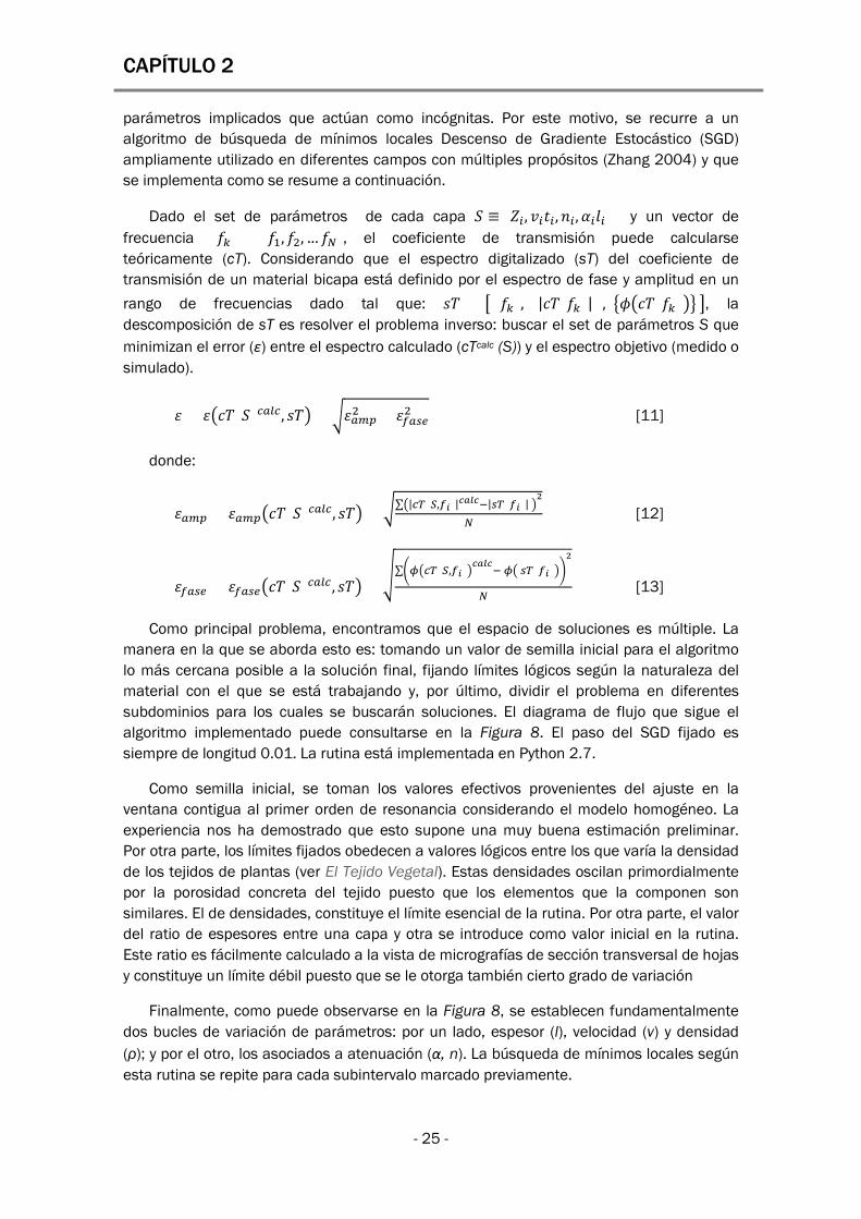
CAPÍTULO 2 parámetros implicados que actúan como incógnitas. Por este motivo, se recurre a un algoritmo de búsqueda de mínimos locales Descenso de Gradiente Estocástico (SGD) ampliamente utilizado en diferentes campos con múltiples propósitos (Zhang 2004) y que se implementa como se resume a continuación.

Dado el set de parámetros de cada capa 𝑆𝑆 ≡ {𝑍𝑍𝑖𝑖, 𝑣𝑣𝑖𝑖𝑡𝑡𝑖𝑖,𝑛𝑛𝑖𝑖,𝑗𝑗𝑖𝑖𝑘𝑘𝑖𝑖} y un vector de frecuencia {𝑓𝑓𝑘𝑘} = {𝑓𝑓1,𝑓𝑓2, … 𝑓𝑓𝑁𝑁}, el coeficiente de transmisión puede calcularse teóricamente (cT). Considerando que el espectro digitalizado (sT) del coeficiente de transmisión de un material bicapa está definido por el espectro de fase y amplitud en un rango de frecuencias dado tal que: 𝑠𝑠𝑇𝑇 = � {𝑓𝑓𝑘𝑘}, {|𝑐𝑐𝑇𝑇(𝑓𝑓𝑘𝑘)| }, �𝜙𝜙�𝑐𝑐𝑇𝑇(𝑓𝑓𝑘𝑘)�� �, la descomposición de sT es resolver el problema inverso: buscar el set de parámetros S que minimizan el error (ε) entre el espectro calculado (cTcalc (S)) y el espectro objetivo (medido o simulado).

𝜀𝜀 = 𝜀𝜀�𝑐𝑐𝑇𝑇(𝑆𝑆)𝑐𝑐𝑐𝑐𝑙𝑙𝑐𝑐, 𝑠𝑠𝑇𝑇� = �𝜀𝜀𝑐𝑐𝑎𝑎𝑎𝑎2 + 𝜀𝜀𝜋𝜋𝑐𝑐𝑠𝑠𝑠𝑠2 [11]

donde:

𝜀𝜀𝑐𝑐𝑎𝑎𝑎𝑎 = 𝜀𝜀𝑐𝑐𝑎𝑎𝑎𝑎�𝑐𝑐𝑇𝑇(𝑆𝑆)𝑐𝑐𝑐𝑐𝑙𝑙𝑐𝑐, 𝑠𝑠𝑇𝑇� = �∑�|𝑐𝑐𝑐𝑐(𝑆𝑆,𝜋𝜋𝑎𝑎)|𝑐𝑐𝑎𝑎𝑙𝑙𝑐𝑐−|𝑠𝑠𝑐𝑐(𝜋𝜋𝑎𝑎)| �2

𝑁𝑁 [12]

𝜀𝜀𝜋𝜋𝑐𝑐𝑠𝑠𝑠𝑠 = 𝜀𝜀𝜋𝜋𝑐𝑐𝑠𝑠𝑠𝑠�𝑐𝑐𝑇𝑇(𝑆𝑆)𝑐𝑐𝑐𝑐𝑙𝑙𝑐𝑐 , 𝑠𝑠𝑇𝑇� =�∑�𝜙𝜙�𝑐𝑐𝑐𝑐(𝑆𝑆,𝜋𝜋𝑎𝑎)�

𝑐𝑐𝑎𝑎𝑙𝑙𝑐𝑐− 𝜙𝜙� 𝑠𝑠𝑐𝑐(𝜋𝜋𝑎𝑎)��2

𝑁𝑁 [13]

Como principal problema, encontramos que el espacio de soluciones es múltiple. La manera en la que se aborda esto es: tomando un valor de semilla inicial para el algoritmo lo más cercana posible a la solución final, fijando límites lógicos según la naturaleza del material con el que se está trabajando y, por último, dividir el problema en diferentes subdominios para los cuales se buscarán soluciones. El diagrama de flujo que sigue el algoritmo implementado puede consultarse en la Figura 8. El paso del SGD fijado es siempre de longitud 0.01. La rutina está implementada en Python 2.7.

Como semilla inicial, se toman los valores efectivos provenientes del ajuste en la ventana contigua al primer orden de resonancia considerando el modelo homogéneo. La experiencia nos ha demostrado que esto supone una muy buena estimación preliminar. Por otra parte, los límites fijados obedecen a valores lógicos entre los que varía la densidad de los tejidos de plantas (ver El Tejido Vegetal). Estas densidades oscilan primordialmente por la porosidad concreta del tejido puesto que los elementos que la componen son similares. El de densidades, constituye el límite esencial de la rutina. Por otra parte, el valor del ratio de espesores entre una capa y otra se introduce como valor inicial en la rutina. Este ratio es fácilmente calculado a la vista de micrografías de sección transversal de hojas y constituye un límite débil puesto que se le otorga también cierto grado de variación

Finalmente, como puede observarse en la Figura 8, se establecen fundamentalmente dos bucles de variación de parámetros: por un lado, espesor (l), velocidad (v) y densidad (ρ); y por el otro, los asociados a atenuación (α, n). La búsqueda de mínimos locales según esta rutina se repite para cada subintervalo marcado previamente.

- 25 -

M.D. FARIÑAS, 2016

Figura 8. Diagrama de flujo que indica el proceso que sigue el algoritmo de Descenso de Gradiente Estocástico (SGD) para el ajuste de un coeficiente de transmisión (cT) dado al modelo cuyos parámetros son li, vi, pi, αi, ni.

cT6dB

Estimación Inicial Imposición de límites n = 0

cT

Divide espacio de búsqueda

Hasta 10 pasos de SGD para li, vi, pi

Hasta 10 pasos SGD para αi, ni

n = n+1

Error en la estimación εn

Guarda la salida Mientras n

= 0 ó εn < ϒ < εn-1

Para cada capa:

li, vi, pi, αi, ni

No Sí

- 26 -

CAPÍTULO 2

- 27 -

2.2. Técnicas Experimentales

2.2.1. Técnicas de Ultrasonidos La electrónica común necesaria para todos los experimentos realizados con

ultrasonidos son un pulser/reciever 5077PR y otro 5058PR, ambos Olympus (Houston, TX, USA) utilizados para llevar la señal al transmisor y para amplificar y filtrar la señal eléctrica proveniente del receptor. También, un osciloscopio digital Tektronix 7054 DPO 500 MHz (Beaverton, OR, USA) con un ordenador integrado en el que corre el software Matlab® (The MathWorks, Natick, MA, USA) que se utiliza para controlar la adquisición de datos, así como para realizar el post-análisis de las señales (transformada de Fourier, ajuste de modelo de una capa, etc.).

La electrónica descrita es precisa en todos los experimentos realizados con ultrasonidos. El elemento fundamental a tener en cuenta a la hora de utilizar una u otra técnica son los transductores ultrasónicos requeridos y la configuración de los mismos.

Figu ra 9. Configuraciones experimentales principales: a, sin contacto y transmisión directa; b, en

contacto y transmisión directa; c, sin contacto y pitch & catch; d, en contacto y pitch & catch.

2.2.1.1. Sin Contacto Como se comentó previamente (ver Espectroscopía Ultrasónica Resonante Sin

Contacto), los transductores (Álvarez-Arenas 2004) ultrasónicos usados en los experimentos en aire, han sido diseñados y fabricados en el laboratorio del CSIC donde se ha desarrollado esta tesis doctoral. Principalmente, se han usado tres pares de

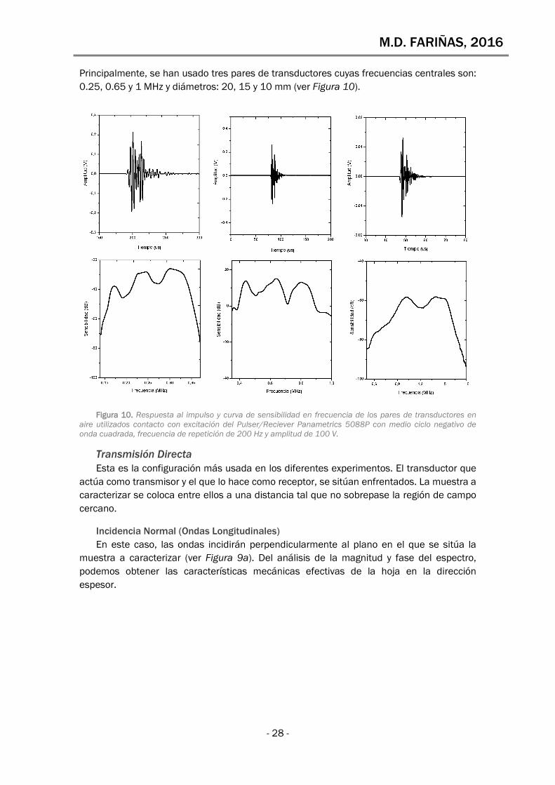
M.D. FARIÑAS, 2016 Principalmente, se han usado tres pares de transductores cuyas frecuencias centrales son: 0.25, 0.65 y 1 MHz y diámetros: 20, 15 y 10 mm (ver Figura 10).

Figura 10. Respuesta al impulso y curva de sensibilidad en frecuencia de los pares de transductores en aire utilizados contacto con excitación del Pulser/Reciever Panametrics 5088P con medio ciclo negativo de onda cuadrada, frecuencia de repetición de 200 Hz y amplitud de 100 V.

Transmisión Directa Esta es la configuración más usada en los diferentes experimentos. El transductor que

actúa como transmisor y el que lo hace como receptor, se sitúan enfrentados. La muestra a caracterizar se coloca entre ellos a una distancia tal que no sobrepase la región de campo cercano.

Incidencia Normal (Ondas Longitudinales) En este caso, las ondas incidirán perpendicularmente al plano en el que se sitúa la

muestra a caracterizar (ver Figura 9a). Del análisis de la magnitud y fase del espectro, podemos obtener las características mecánicas efectivas de la hoja en la dirección espesor.

- 28 -

CAPÍTULO 2

Figura 11 Fotografía de las pinzas de transductores ultrasónicos empleadas para medir en transmisión directa e incidencia norma y cuyas características aparecen en la Figura 10.

Incidencia Oblicua (Ondas de Cizalla) La disposición de los transductores es similar a la anterior, pero la muestra se coloca

con la ayuda de un goniómetro de tal manera que la onda incide con un ángulo de entre 5º y 40º con respecto a su plano normal. En esta configuración, se excitarán no únicamente ondas longitudinales como en incidencia normal, sino también ondas de cizalla. Las ondas de cizalla se producen en dirección perpendicular a la de propagación y contendrán información sobre el módulo de cizalladura del material. Estas ondas son más lentas que las longitudinales y en el caso de los tejidos vegetales aparecen altamente atenuadas. Por ello, en muchas ocasiones no serán visibles en el espectro medido experimentalmente.

Pitch & Catch

Incidencia Oblicua (Ondas Guiadas) Esta configuración corresponde con la Figura 9c. Las ondas propagadas serán ondas

guiadas a lo largo del plano de la muestra, excitadas por el principio de coincidencia (Cremer 1947). Este particular tipo de ondas se propaga por el material cuando la onda incide con un ángulo superior al crítico, y contiene información de todo el volumen de la muestra propagado hasta la posición en que se detecte en el receptor. Los transductores usados en este caso son los que aparecen en la Figura 12.

2.2.1.2. Con Contacto En esta ocasión, los transductores usados son en su mayoría comerciales (Panametrics

/ Olympus). Para asegurar el perfecto acoplamiento entre la superficie del transductor y la muestra, se utiliza gel acoplante (Olympus).

- 29 -

M.D. FARIÑAS, 2016

Transmisión Directa

Incidencia Normal: Ondas Longitudinales Un par de transductores de 1 MHz (V314, Panametrics) se colocaron perfectamente

enfrentados y adheridos a la hoja usando el gel acoplante. Del desfase entre el tiempo de llegada de la señal sin muestra entre transductor y receptor y con ella, junto con el espesor de la hoja, se puede obtener la velocidad ultrasónica (ver Figura 9b).

Incidencia Normal: Ondas de Cizalla En este caso, el transductor utilizado genera ondas linealmente polarizadas con

frecuencia central 2.25 MHz (V154, Panametrics). Otra peculiaridad de esta técnica, es que el gel acoplante es específico para ondas de cizalla, de alta viscosidad. Obtendremos las dos velocidades de onda de corte que se propagan por la hoja a consecuencia de las dos posibles combinaciones de la polaridad (ver Figura 9b).

Pitch & Catch Dos transductores de frecuencia central 0.25 MHz fabricados en el CSIC se acoplarán

esta vez en el mismo lado de la hoja separados unos centímetros (ver Figura 12). El receptor se irá moviendo con el fin de escanear mayor distancia y calcular la velocidad de propagación del sonido por las fibras longitudinales de la hoja (ver Figura 9d).

Figura 12 Respuesta al impulso y curva de sensibilidad en frecuencia del par de transductores de 0.25 MHz en contacto con excitación del Pulser/Reciever Panametrics 5077 con medio ciclo negativo de onda cuadrada centrada en 250 kHz; amplitud 100 V y recepción -19 dB.

2.2.2. Otras Técnicas

2.2.2.1. Medidas de Espesor y Densidad Durante el desarrollo de los experimentos, se tomaron numerosas medidas

independientes del espesor de las hojas, con la ayuda de un micrómetro comercial (Mitutoyo ±0.01 mm). Paralelamente, se extrajeron discos del material con la ayuda de un sacabocados (14 mm de diámetro - cuando el área de la hoja lo permitía -) y se pesaron en una báscula de precisión (Precisa XT 220A ±0.001 g). Se calcularon posteriormente las densidades de las muestras.

- 30 -

CAPÍTULO 2

2.2.2.2. Curvas de Presión – Volumen Las curvas de presión-volumen fueron determinadas usando la cámara de presión tipo

Scholander (Brodribb y Holbrook 2003). Básicamente, el método consiste en, una vez tomada la muestra, incrementar la presión alrededor de la hoja mientras el peciolo, previamente escindido del resto de la planta, permanece a presión atmosférica. La presión aplicada para hacer que una gota de agua salga al exterior desde el peciolo, será la que marque la presión del agua en la hoja.

2.2.2.3. Contenido Relativo de Agua en la Hoja El contenido hídrico relativo (RWC) representa la cantidad de agua de un tejido en

comparación a su estado de hidratación plena. Para obtenerlo, se pesa la muestra en su estado de plena turgencia, se vuelve a pesar en un instante dado y, al finalizar el experimento, se seca en el horno a 80 ºC durante 48 horas, y se vuelve a pesar para obtener el peso seco.

2.2.2.4. Conductividad Estomática La conductividad estomática (gs) da idea de la actividad en la hoja. Particularmente,

representa el flujo de C02 y humedad entre el medio interno y externo a ella. Este intercambio se produce a través de los estomas, que son unos pequeños poros situados en el tejido epidérmico foliar, concretamente en el envés. La apertura y cierre de estomas está regulado por las células de guarda, que actúan ante determinadas condiciones medioambientales en relación con el estado de la hoja. El porómetro comercial utilizado fue el SC-1 de Decagon Devices (Pullman, WA, USA).

2.2.2.5. Sensores Comerciales Sensores de tensión de suelo (Watermark 200SS-V; Irrometer, Riverside, CA, USA), de

intensidad de luz (SQ-200-5; Apogee Instruments, Logan, UT, USA) y de temperatura en aire y en suelo han sido utilizados también en diversos experimentos recogidos en los artículos anexados.

2.2.2.6. Imagen

Microscopía Óptica Un microscopio Leica DM 750 equipado con una cámara ICC50 HD se ha usado para

obtener imágenes de cortes transversales de hojas en fresco. Para realizar los cortes, se empleó un micrótomo de mesa Allmikro. Posteriormente, de cara a analizar medidas de los tejidos en el corte transversal, se han analizado las imágenes usando el software ImageJ (National Institutes of Health, Bethesda, MD, USA).

Microscopía Electrónica de Barrido por Congelación Se tomaron imágenes de los cortes transversales de hojas usando microscopía

electrónica de barrido por congelación. Como principal ventaja frente a la microscopía óptica, más allá de la resolución, brinda la oportunidad de captar diferentes estados de hidratación de la hoja fácilmente. Para este fin, se usó un LTSEM, DSM 960 Zeiss (Alemania) con aceleración potencial de 15 kV, distancia de trabajo de 10 mm y corriente de 5-10 nA. Se realizaron los cortes transversales de la hoja en fresco (al estado concreto de hidratación que se pretendía fotografiar), se sumergieron en nitrógeno líquido, se fracturaron y se pulverizó oro sobre su superficie para convertirla en conductora.

- 31 -

M.D. FARIÑAS, 2016

- 32 -

CAPÍTULO 3

CAPÍTULO 3.Propagación de Ondas de

Cizalla en Tejidos Vegetales mediante la

técnica NC-RUS

- 33 -

M.D. FARIÑAS, 2016

- 34 -

“L’etude approfondie de la nature est la source la plus féconde des découvertes mathématiques. Non seulement cette étude, en offrant aux recherches un but determine, a l’avantage d’exclure les questions vagues et les calculs sans issue; elle est encore un moyen assuré de former l’analyse elle même, et d’en découvrir les éléments fondamentaux sont ceux qui se reproduisent dans tous les effets natureles.”

Jean Baptiste Joseph Fourier

Discours préliminaire. La théorie Analytique de la Chaleur, p. 7. 1822.

CAPÍTULO 3

En este capítulo, se busca conocer los parámetros ultrasónicos característicos de cada capa de la hoja tanto en su componente longitudinal como transversal, así como la variación de estos con el contenido de agua empleando la técnica NC-RUS. El estudio de la propagación de ondas de cizalla en tejidos vegetales supone un avance novedoso no contemplado en la literatura previa. Asimismo, estos trabajos suponen una primera aproximación a la aplicación del modelo acústico de dos capas en la hoja.

En primer lugar, se incluye la publicación en revista científica cuya referencia es:

FARINAS, M.D., SANCHO-KNAPIK, D., PEGUERO-PINA, J.J., GIL-PELEGRIN, E. y ALVAREZ-ARENAS, T.E.G., 2013. Shear waves in vegetal tissues at ultrasonic frequencies. Applied Physics Letters [en línea], vol. 102, no. 10, pp. 103702. [Consulta: 5 abril 2013]. ISSN 00036951. DOI 10.1063/1.4795785. Disponible en:http://link.aip.org/link/APPLAB/v102/i10/p103702/s1&Agg=doi.

En segundo lugar, se incluye el trabajo presentado en congreso internacional cuya referencia es:

FARIÑAS, M.D., ALVAREZ-ARENAS, T.E.G., SANCHO-KNAPIK, D., PEGUERO-PINA, J.J. y GIL-PELEGRIN, E., 2012. Shear waves in plant leaves at ultrasonic frequencies: Shear properties of vegetal tissues. 2012 IEEE International Ultrasonics Symposium. S.l.: IEEE, pp. 1513-1516. ISBN 978-1-4673-4562-0. DOI 10.1109/ULTSYM.2012.0378 Disponible en: http://ieeexplore.ieee.org/xpl/freeabs_all.jsp?arnumber=6562227&abstractAccess=no&userType=inst

- 35 -

M.D. FARIÑAS, 2016

- 36 -

Shear waves in vegetal tissues at ultrasonic frequenciesM. D. Fariñas, D. Sancho-Knapik, J. J. Peguero-Pina, E. Gil-Pelegrín, and T. E. Gómez Álvarez-Arenas

Citation: Appl. Phys. Lett. 102, 103702 (2013); doi: 10.1063/1.4795785 View online: http://dx.doi.org/10.1063/1.4795785 View Table of Contents: http://apl.aip.org/resource/1/APPLAB/v102/i10 Published by the American Institute of Physics.

Additional information on Appl. Phys. Lett.Journal Homepage: http://apl.aip.org/ Journal Information: http://apl.aip.org/about/about_the_journal Top downloads: http://apl.aip.org/features/most_downloaded Information for Authors: http://apl.aip.org/authors

Downloaded 05 Apr 2013 to 161.111.29.122. This article is copyrighted as indicated in the abstract. Reuse of AIP content is subject to the terms at: http://apl.aip.org/about/rights_and_permissions

- 37 -

Shear waves in vegetal tissues at ultrasonic frequencies

M. D. Fari~nas,1 D. Sancho-Knapik,2 J. J. Peguero-Pina,2 E. Gil-Pelegr�ın,2 andT. E. G�omez �Alvarez-Arenas1,a)

1UMEDIA research group, Spanish National Research Council, CSIC, Madrid, Spain2Unidad de Recursos Forestales, CITA, Gobierno de Arag�on, Zaragoza, Spain

(Received 12 November 2012; accepted 5 March 2013; published online 15 March 2013)

Shear waves are investigated in leaves of two plant species using air-coupled ultrasound.

Magnitude and phase spectra of the transmission coefficient around the first two orders of the

thickness resonances (normal and oblique incidence) have been measured. A bilayer acoustic

model for plant leaves (comprising the palisade parenchyma and the spongy mesophyll) is

proposed to extract, from measured spectra, properties of these tissues like: velocity and

attenuation of longitudinal and shear waves and hence Young modulus, rigidity modulus, and

Poisson’s ratio. Elastic moduli values are typical of cellular solids and both, shear and longitudinal

waves exhibit classical viscoelastic losses. Influence of leaf water content is also analyzed. VC 2013American Institute of Physics. [http://dx.doi.org/10.1063/1.4795785]

Generation and propagation of shear waves in animal

tissues and organs have already been used by different char-

acterization, test, and imaging techniques. They are com-

monly used in the transient elastography, the supersonic

shear wave elastography, and the elastography using acoustic

radiation force.1,2 A large number of medical applications

are currently being developed and investigated based on the

fact that mechanical properties of soft tissues change

depending on the state of diseases like breast cancer, hepatic

fibrosis, or thrombosis. The working frequency is typically

between 50 and 1000 Hz. Young modulus of these soft

tissues use to be very low (between 17 Pa for fat and up to

300 MPa for the Aquilles’ tendon3).

For vegetal tissues, there is an increasing interest in the

study of tissues’ elasticity: understanding the interaction of

the plant with the external mechanical stimuli,4 mathemati-

cal modeling of the role of internal mechanical tensions in

cell proliferation and plant patterns formation,5 manufactur-

ing of synthetic nano-composites using plant primary cell

walls,6 and non-invasive sensing of plants watering needs.7

Unlike animal cells, vegetal cells are surrounded by a cell

wall. In the past, this wall was viewed as an inanimate rigid

scaffold, but it is now recognized as a dynamic structure that

plays an important role in controlling the development of the

plant and the adaptation to the environment.8,9 One of its

functions is to withstand the osmotic pressure of the cell. So,

the combination of cell pressure and cell wall strength con-

tributes to the whole rigidity of plants. Cell walls may differ

in function and in composition. The walls surrounding grow-

ing and dividing plant cells must provide mechanical

strength but must also expand to allow the cell to grow and

divide. Once the cell has ceased to grow, a much thicker and

stronger wall may then develop.9 In general, cell wall

accounts for most of the carbohydrate in biomass. In addi-

tion, it may have a major impact on human life, as it is a

major component of wood, a source of nutrition for live-

stock, and account for the bulk of renewable biomass that

can be converted to fuel out of a plant. These features sug-

gest that it might be possible to observe the propagation of

shear waves in plant tissues at ultrasonic frequencies and

that this can provide valuable information, which may have

significant economic implications.

Some ultrasonic techniques using longitudinal waves

have been applied in the past to study plant leaves.10,11 More

recently, air-coupled ultrasound and normal incidence have

been used to excite and sense thickness resonances in plant

leaves to obtain in a non invasive and a nondestructive way

valuable information about plant status.7,12,13 Although a

similar technique, but using oblique incidence, has been con-

ventionally used to generate and sense shear waves in other

materials,14 no evidence of the appearance of shear waves at

ultrasonic frequencies in plant leaves has been previously

reported for some species.7 The purpose of this paper is

to study shear waves in plant leaves using a broadband

air-coupled ultrasonic technique and normal and oblique

incidence. Properties of the leaf tissues are extracted from

the measured spectra using a bilayer acoustic model.

Three pairs of air-coupled and wide band ultrasonic

transducers were used in a through transmission experimen-

tal set-up (transmitter-receiver separation of 45 mm), center

frequencies are 0.25, 0.70, and 1.00 MHz, usable bandwidths

0.15–0.35 MHz, 0.35–0.90 MHz, and 0.60–1.50 MHz, and

sensitivities �25 dB, �29 dB, and �35 dB, respectively.

Transmitter transducer is driven by a Panametrics 5058

pulser. The received signal is amplified 40 dB, high-pass fil-

tered (0.03 MHz), and digitized by a Tektronix 7054 digital

oscilloscope. Angle of incidence is controlled by a goniome-

ter. Magnitude and phase spectra of the transmission coeffi-

cient are measured for all leaves varying the angle of

incidence from 0� to 40� in steps of 5� (see Figs. 1–3). At

normal incidence, shear wave generation does not take place

and transmission coefficient is defined by the pattern of the

thickness resonances, which is produced by the longitudinal

wave and the finite leaf dimensions. As the angle of inci-

dence increases, part of the particle displacement produced

by the incident ultrasound field on the leaf surface takes

place on the plane of the leaf, shear displacements are

a)Author to whom correspondence should be addressed. Electronic mail:

tgomez@ia.cetef.csic.es.

0003-6951/2013/102(10)/103702/5/$30.00 VC 2013 American Institute of Physics102, 103702-1

APPLIED PHYSICS LETTERS 102, 103702 (2013)

Downloaded 05 Apr 2013 to 161.111.29.122. This article is copyrighted as indicated in the abstract. Reuse of AIP content is subject to the terms at: http://apl.aip.org/about/rights_and_permissions

- 38 -

generated, and consequently, mode conversion takes place

and shear waves are generated. As the angle of incidence

increases, more energy is coupled into the shear mode. This

shear wave also reverberates within the leaf and produces a

pattern of thickness resonances. As long as measurements

are taken at an angle below the limit angle for longitudinal

waves, this shear wave resonances overlaps to the pattern of

thickness resonances due to the longitudinal wave (see Figs.

2 and 3), so what we observe is the overlap or interference of

these two patterns of thickness resonances: longitudinal and

shear (see also Ref. 14).

For comparison purposes, longitudinal and shear wave

velocities were also obtained from conventional time of

flight measurements using a through transmission technique

with direct contact and commercial shear-wave and

longitudinal-wave transducers (0.5 MHz, Panametrics). To

efficiently couple shear-wave transducer to the leaves, a

commercial shear wave coupling gel was used.

Leaves from different species were tested, in many cases,

no shear waves were observed (e.g., Platanus hispanica,

Ligustrum lucidum, Prunus laurocerasus, and immature—

spring time—Vitis vinifera leaves). This can be attributed to a

very high attenuation coefficient of shear waves in these leaves.

However, in some other cases, shear waves were clearly seen.

This paper focuses on leaves of Epipremnum aureum and

mature (summer time) leaves of V. vinifera, where shear waves

were observed. Another reason to select these species is that

they correspond to two extreme cases from the point of view

of the bilayer acoustic model: the two layers of E. aureumleaves are strongly different while they are very similar for

V. vinifera leaves. Ten leaves of V. vinifera were collected

and preserved according to the procedure in Ref. 7. Ten

FIG. 1. Magnitude and phase spectra of the transmission coefficient at

normal incidence. � and �: measured magnitude and phase spectra, respec-

tively. Dashed line: theoretical predictions of the one-layer model (V. vinifera:

vL¼ 341 m/s, q¼ 866 kg/m3, t¼ 256 lm, aL0 ¼ 991 Np/m, fres¼ 659 kHz, and

n¼ 1.75. E. aureum: vL¼ 194 m/s, q¼ 894 kg/m3, t¼ 391lm, aL0 ¼ 590 Np/m,

fres¼ 246 kHz, and nL¼ 1.75). Solid line: theoretical predictions of the bilayer

model (V. vinifera: vLPP¼ 450 m/s, vL

SM ¼ 300 m/s, qPP¼ 952 kg/m3,

qSM¼ 779 kg/m3, tPP ¼ tSM ¼ 128 lm, aLPP0¼ aL

SM0¼ 940 Np/m, and nL¼ 1.8. E. aureum: vL

PP¼ 400 m/s, vLSM ¼ 175 m/s, qPP¼ 1254 kg/m3,

qSM¼ 444 kg/m3, tPP ¼ tSM ¼ 195 lm, aLPP0¼ aL

SM0 ¼ 451 Np/m, and nL¼ 2).

FIG. 2. Magnitude and phase spectra of the transmission coefficient versus

frequency for a E. aureum leaf at three angles of incidence (10�, 20�, and

30�). � and �: measured magnitude and phase spectra, respectively. Solid

lines (blue and red): calculated magnitude and phase spectra using the

bilayer model, respectively. Data for the calculations are in Fig. 1 caption to-

gether with the following shear wave data: Poisson’s ratio¼ 0.33 (this

implies vSHPP ¼ 200 m/s and vSH

SM ¼ 88 m/s), aSH0 ¼ 924 Np/m, and nSH¼ 2.

Longitudinal thickness resonance appears at 248 kHz and the interference

with the shear wave resonance appear (for incidence angle> 15�) close to

300 kHz.

FIG. 3. Magnitude and phase spectra of the transmission coefficient versus

frequency for a V. vinifera leaf at three angles of incidence (10�, 20�, and 30�).� and �: measured magnitude and phase spectra, respectively. Solid lines

(blue and red): calculated magnitude and phase spectra using the bilayer

model, respectively. Data for the calculations are tPP ¼ tSM ¼ 147lm,

fres¼ 531 kHz, vLPP¼ 500 m/s, vL

SM ¼ 274 m/s, qPP¼ 950 kg/m3, qSM

¼ 680 kg/m3, aL0 ¼ 750 Np/m, nL¼ 2, Poisson’s ratio¼ 0.34 (this implies

vSHPP ¼ 245 m/s, vSH

SM ¼ 134 m/s), aSH0 ¼ 1500 Np/m, and nSH¼ 2. The interfer-

ence with the shear wave resonance appears (for incidence angle> 15�) close

to 650 kHz.

103702-2 Fari~nas et al. Appl. Phys. Lett. 102, 103702 (2013)

Downloaded 05 Apr 2013 to 161.111.29.122. This article is copyrighted as indicated in the abstract. Reuse of AIP content is subject to the terms at: http://apl.aip.org/about/rights_and_permissions

- 39 -

leaves of E. aureum were measured directly from the plant

without cutting them.

To theoretically analyze the presence of shear waves in

the transmission coefficient spectra, the analysis cannot be

limited to the vicinity of the first thickness resonance but

must include a larger frequency window.7,15 This requires

that the layered structure of the leaf must be considered, in

other words, the one-layer effective model used in previous

works cannot be used now (see Fig. 1).

The mathematical model considered here for plant

leaves consists of a stack of two layers of different tissues

(bilayer model). The first layer (PP-layer) comprises the

upper epidermis and the palisade parenchyma (PP) while

the second one (SM-layer) comprises the spongy mesophyll

(SM) and the lower epidermis. The cells of the parenchyma

tissues are densely packed together: they can be thought of

as a pressurized, liquid-filled closed-cell foam,9 with an

effective density close to the density of its main constitu-

ents: water (1000 kg/m3), cellulose (1500 kg/m3), ligning

(1300 kg/m3), and wax (950 kg/m3). The SM layer can also

be considered a cellular material, but with a relatively

higher porosity and open-cell structure for it must allow the

gaseous interchange with the surrounding air. Thicknesses

of these two layers are considered equal,16,17 and also the

attenuation coefficient and the Poisson’s ratio.

First, the one-layer model is employed to extract effec-

tive leaf properties from measurements at normal incidence

in the vicinity of the first resonance as explained in Ref. 12.

In all cases, it is assumed that velocity does not change with

the frequency (f) and that attenuation coefficient (aL and aSH,

for longitudinal and shear waves, respectively) follows a

power law as it has been done in the past for a large number

of porous materials and biological tissues18

aL ¼ aL0ð f=fresÞnL;

aSH ¼ aSH0 ð f=fresÞnSH;

(1)

where fres is the frequency of the first thickness resonance.

Figure 1 shows measurements of the transmission coeffi-

cient spectra at normal incidence. Leaf effective properties

obtained using the one layer model13 (see Fig. 1 caption) are

used as initial values for the bilayer model. Then, we only

allow to change velocity and density of the PP and the SM

layers (they become stepwise more different, i.e., anisotropy

between layers is increased) until the fitting of the theoreti-

cally calculated transmission coefficient into the experimen-

tal data over the whole frequency range reaches an optimum

value. Results are also shown in Fig. 1.

Once these data are determined, the magnitude and the

phase spectra of the transmission coefficient at oblique inci-

dence are theoretically calculated using the set of parameters

obtained at normal incidence and only changing the Poisson

ratio, from �1 to 0.5 in steps of 0.01. Negative Poisson’s ra-

tio values were considered because such values have been

previously reported for some vegetal tissues.19 The purpose

is to theoretically reproduce the frequency location of the

shear wave interference. Once this is achieved, shear wave

attenuation is changed until the calculated amplitude of this

interference matches the experimental value. Results for

three angles of incidence are shown in Figures 2 and 3, the

appearance of the shear wave is clear for incidence angles

beyond 10�. Although there is little information about the

Poisson ratio in vegetal tissues, obtained values here (0.33

and 0.34) agree with available estimations: 0.28 (lignin),

0.18–0.4 (onion epidermis), and 0.23–0.5 (parenchyma

tissues).5,20–23 The fact that nL and nSH are close to 2 con-

firm that the main source of losses have a classical visco-

elastic origin with the condition that xs � 1, where s is a

relaxation time that characterizes the medium and x the

angular frequency.

With the purpose to confirm these results, longitudinal

and shear wave velocities were measured using a direct con-

tact, through transmission technique at 0.5 MHz. In this case,

the results are affected by a relatively large uncertainty due

to the irregularities of the leaf surfaces and the difficulty to

efficiently attach the transducers to them. Ten leaves of each

species were measured at three different points. Averaged

data and standard deviations are shown in Table I. For com-

parison purposes, average values hvLi ¼ ðvLPP þ vL

SMÞ=2�

and

hvSHi ¼ ðvSHPP þ vSH

SMÞ=2Þ. obtained by the air-coupled tech-

nique and the bilayer model are also shown.

From these data, elastic moduli can be worked out,

results are summarized in Table II.

These values are similar to data reported before for veg-

etable tissues (e.g., Young modulus of 8–19 MPa for paren-

chyma cells, 2–22 MPa for aerenchyma and collenchyma

cells, respectively,9,19,24 and 50–200 MPa for Quercus

leaves;21 and modulus of rigidity between 2 and 22 MPa

(Ref. 25)). At normal or high turgor pressures, the cell walls

are taut, and deformation is dominated by stretching of the

cell walls. The Young’s modulus of the parenchyma tissue

(Etissue) is then directly proportional to its relative density

(which is equivalent to the volume fraction of solids: /s)9

Etissue / Ecw/s; (2)

where Ecw is Young modulus of the cell wall. So, measured

Etissue values can be used to compare the microstructure of

different parenchyma tissues or parenchyma tissues from

TABLE I. Longitudinal, vL, and shear, vSH , wave velocities (m/s) in the

leaves obtained by the two different experimental methods.

Gel coupling Air-coupled spectroscopy

vL vSH hvL i hvSHi

E. aureum 320 6 27 180 6 18 290 6 15 145 6 10

V. vinifera 460 6 50 155 6 17 390 6 15 190 6 10

TABLE II. Elastic moduli of the leaf tissues.

Tissue E (MPa) G (MPa)

V. vinifera PP 150 6 5 60 6 3

SM 30 6 3 12 6 1

E. aureum PP 135 6 5 50 6 2

SM 9 6 1 3 6 0.5

103702-3 Fari~nas et al. Appl. Phys. Lett. 102, 103702 (2013)

Downloaded 05 Apr 2013 to 161.111.29.122. This article is copyrighted as indicated in the abstract. Reuse of AIP content is subject to the terms at: http://apl.aip.org/about/rights_and_permissions

- 40 -

different species by comparing the value of the proportion-

ally constants in Eq. (2).

It is worthwhile noting that the appearance of shear

waves in V. vinifera strongly depends on the leaf degree

of development. For leaves collected at spring time,

aL0 > 1000 Np/m, there is no evidence of the shear waves. On

the contrary, for leaves collected during summer and fall,

aL0 � 750 Np/m, the shear wave is clearly detected. This can

be produced by the further evolution and stiffening of the

cell wall produced when the leaf growth is finished.8,9

Finally, the influence of leaf water content was studied.

Towards this end, leaf weight and magnitude and phase spec-

tra of the transmission coefficient at an incidence angle of

30� were measured in leaves cut at full saturation and then

left to dry at room conditions. Measurements were taken ev-

ery 3 min during 3 h. Once finished, the leaves were fully

dried in a stove at 70� during 24 h to obtain the leaf dry

weight and then the leaf relative water content (RWC).17

The variation with RWC in the measured longitudinal thick-

ness resonance frequency (fres) and in the other PP-layer pa-

rameters extracted from the measurements is shown in

Figure 4. Variation in fres with RWC follows a sigmoid

behavior as reported before for other species measured at

normal incidence15 and the point of turgor loss can be deter-

mined from the location of the point of inflection: RWC0.

The exact location of this point of inflection is calculated by

fitting the logistic curve (Eq. (3)) into the experimental data

(RWC0¼ 0.935).

y ¼ y0 þ ðyF � y0Þ.�

1þ�ðRWC=RWC0Þ

�p�; (3)

where superscripts 0 and F denote the full water saturation

and the final (dry) states, respectively. vLPP and aL

PP vs. RWC

also follow a sigmoid variation, and it is possible to fit the

logistic curve (Eq. (3)) into these measurements, obtained

points of inflection are also shown in Fig. 4 and are very

close to RWC0.

Shear properties (vSHPP and aSH

PP) and Poisson’s ratio does

not follow a sigmoid evolution with RWC. Attenuation con-

tinues increasing beyond the turgor loss point while velocity

keeps on decreasing. Another feature found in shear waves,

and not in longitudinal waves, is the initial high rate of varia-

tion in vSHPP with RWC. These features are reflected in the var-

iation in the Poisson’s ratio with RWC that presents two

transitions one at the very beginning of the desiccation pro-

cess (RWC¼ 0.99) and the other close to RWC0.

All these features can be explained by the overall loss of

rigidity and the increase of compressibility in the vegetal tis-

sues when water content is reduced due to the decay of the

pressure of the cells against the cell wall: cell wall is no lon-

ger taut and deformation takes place by bending. In addition,

it is observed that while the shear velocity keeps decreasing

beyond the turgor loss point (and, hence, also G), the longi-

tudinal velocity reaches a limit value (consequently, also the

modulus of compressibility K: vL ¼ffiffiffiffiffiffiffiffiffiffiffiffiffiffiffiffiffiffiffiffiffiffiffiffiffiffiffiffiffiðK þ 4=3GÞ=q

p).

In summary, this work demonstrates the feasibility of prop-

agate and detect shear waves in plant leaves in a completely

non-invasive way using wideband air-coupled ultrasonic pulses

and a bilayer model for the leaf to extract leaf parameters from

measured spectra, and reveals the potential use of this technique

to study the elasticity of the different vegetal tissues and their

variations due to leaf development or to water content changes.

Financial support from Spanish MINECO through

Project DPI 2011-22438 is acknowledged.

1L. S. Wilson, D. E. Robinson, and M. J. Dadd, Phys. Med. Biol. 45(6),

1409 (2000).2M. Tanter, J. Bercoff, A. Athanasiou, T. Deffieux, J.-L. Gennison, G.

Montalvo, M. Muller, A. Tardivon, M. Fink, Ultrasound Med. Biol. 34(9),

1373 (2008).3I. Levental, P. C. Georges, and P. A. Janmey, Soft Matter 3(3), 299

(2007).4F. W. Telewski, Am. J. Bot. 93(10), 1466 (2006).5A. C. Newell and P. D. Shipman, J. Stat. Phys. 121(5–6), 937 (2005); R.

Kennaway, E. Coen, A. Green, and A. Bangham. PLoS Comput. Biol.

7(6), e1002071 (2011).6D. M. Bruce, R. N. Hobson, J. W. Farrent, and D. G. Hepworth,

Composites, Part A 36(11), 1486 (2005); A. P. Kumar, D. Depan, N.

Singh Tomer, and R. P. Singh, Prog. Polym. Sci. 34(6), 479 (2009).7T. E. G�omez �Alvarez-Arenas, D. Sancho-Knapik, J. J. Peguero-Pina, and E.

Gil-Pelegr�ın, Appl. Phys. Lett. 95(19), 193702 (2009); D. Sancho-Knapik,

T. G�omez �Alvarez-Arenas, J. J. Peguero-Pina, and E. Gil Pelegr�ın, J. Exp.

Bot. 61(5), 1385 (2010).8D. J. Cosgrove, Nat. Rev. Mol. Cell Biol. 6(11), 850 (2005).9L. J. Gibson, J. R. Soc., Interface 9(76), 2749 (2012).

10M. Fukuhara, Plant Sci. 162(4), 521 (2002).11P. S. Wilson and K. H. Dunton, J. Acoust. Soc. Am. 125(4), 1951 (2009).12D. Sancho-Knapik, T. G. �Alvarez-Arenas, J. J. Peguero-Pina, V.

Fern�andez, and E. Gil-Pelegr�ın, J. Exp. Bot. 62(10), 3637 (2011).13D. Sancho-Knapik, H. Cal�as, J. J. Peguero-Pina, A. Ramos Fernandez, E.

Gil-Pelegr�ın, and T. E. G�omez Alvarez-Arenas, IEEE Trans. Ultrason.

Ferroelect. Freq. Control 59(2), 319 (2012).14T. E. G�omez �Alvarez-Arenas, F. Montero, M. Moner-Girona, E.

Rodr�ıguez, A. Roig, and E. Molins, Appl. Phys. Lett. 81(7), 1198 (2002).

FIG. 4. Variation in the properties of the PP-layer of a E. aureum leaf during

dehydration. Solid lines: fitting of the logistic function (Eq. (3)) into the cor-

responding experimental data. Vertical dashed lines indicate the location of

the point of inflection of the solid-line curves. Fig. 4(a) �: Variation in fres

(left vertical axis) with RWC; Relative variation in the attenuation coeffi-

cient (right vertical axis) with RWC. � (blue): DaL=aL0 and � (red):

DaSH=aSH0 . Fig. 4(b) �: Variation in the Poisson’s ratio (right vertical axis)

with RWC; Relative variation in the velocity (left vertical axis) with RWC.

� (blue): DvSHPP=vSH

PP and � (red): DvLPP=vL

PP.

103702-4 Fari~nas et al. Appl. Phys. Lett. 102, 103702 (2013)

Downloaded 05 Apr 2013 to 161.111.29.122. This article is copyrighted as indicated in the abstract. Reuse of AIP content is subject to the terms at: http://apl.aip.org/about/rights_and_permissions

- 41 -

15T. E. G�omez �Alvarez-Arenas, D. Sancho-Knapik, J. J. Peguero-Pina, and

E. Gil Pelegrin, in 2009 IEEE International Ultrasonics Symposium, Rome(2009), pp. 771–774.

16H. Toshoji, T. Katsumata, M. Takusagawa, Y. Yusa, and A. Sakai,

Protoplasma 249(3), 805 (2012).17A. Ben Salem-Fnayou, B. Bouamama, A. Ghorbel, and A. Mliki, Microsc.

Res. Tech. 74(8), 756 (2011).18T. Szabo, J. Acoust. Soc. Am. 96, 491 (1994).19K. J. Niklas, Plant Biomechanics (The University of Chicago Press,

London, 1992).

20T. J. Brodribb and N. M. Holbrook, Plant Physiol. 137, 1139 (2005).21T. Saito, K. Soga, T. Hoson, and I. Terashima, Plant Cell Physiol. 47(6),

715 (2006).22C. Wei, P. M. Lintilhac, and J. J. Tanguay, Plant Physiol. 126(3), 1129

(2001).23E. Vanstreels, M. C. Alamar, B. E. Verlinden, A. Enninghorst, J. K. A.

Loodts, E. Tijskens, H. Ramon, and B. M. Nicola€ı, Postharvest Biol.

Technol. 37(2), 163 (2005).24J. Blahovec, J. Mater. Sci. 23(10), 3588 (1988).25I. Burgert, Am. J. Bot. 93(10), 1391 (2006).

103702-5 Fari~nas et al. Appl. Phys. Lett. 102, 103702 (2013)

Downloaded 05 Apr 2013 to 161.111.29.122. This article is copyrighted as indicated in the abstract. Reuse of AIP content is subject to the terms at: http://apl.aip.org/about/rights_and_permissions

- 42 -

Shear Waves in Plant Leaves at Ultrasonic Frequencies: Shear properties of Vegetal Tissues.

M.D. Fariñas and T.E.Gómez Álvarez-ArenasUMEDIA research group.

Spanish Scientific Research Council, CSICMadrid, Spain

tgomez@ia.cetef.csic.es

D. Sancho-Knapik, J. J. Peguero-Pina and E. Gil-Pelegrín

Unidad de Recursos Forestales CITA, Gobierno de Aragón

Zaragoza, Spain

Abstract— Shear Waves are observed in leaves of some plant species (Epipremnum aureum and Vitis vinifera) using air-coupled ultrasound, through transmission and oblique incidence. Shear waves appear as a modification of the thickness resonance pattern of the longitudinal wave measured at normal incidence. Poisson’s ratio, shear wave velocity and attenuation coefficient of shear waves in the leaves are extracted from the measured resonance spectra using a bilayer acoustic model for the leaves. Influence of water content or the degree of leaf development on shear wave properties is also analyzed.

Keywords-component; air-coupled ultrasound, shear waves, organic tissues, plant leaves.

I. INTRODUCTION.Generation and propagation of shear waves in animal

tissues and organs have already been used by different characterization, test and imaging techniques. Elastography is a well known example with a large number of medical applications. Reviews of this technique can be seen in [1] and [2].

Unlike animal cells, vegetal cells are surrounded by a cell wall. In the past, this wall was viewed as an inanimate rigid scaffold, but it is now recognized as a dynamic structure that plays an important role in controlling the development of the plant [3]. One of its functions is to withstand the osmotic pressure of the cell. So, the combination of cell pressure and cell wall strength contributes to the whole rigidity of a plant. Cell walls may differ in function and in composition. Walls surrounding growing and dividing plant cells must provide mechanical strength but must also expand to allow the cell to grow and divide. Once the cell has ceased to grow, a much thicker and stronger wall may then develops. In general, cell wall accounts for most of the carbohydrate in biomass. In addition, they may have a major impact on human life, as they are a major component of wood, are a source of nutrition for livestock and account for the bulk of renewable biomass that can be converted to fuel out of a plant.

So, as cell walls provide a relatively larger rigidity to vegetal tissues compared with animal ones, then relatively larger modulus of rigidity, lower viscosities and, consequently, faster propagation velocities and lower attenuation coefficients are expected. These features suggest that it might be possible to observe the propagation of shear waves in plant tissues at

ultrasonic frequencies and that this can provide valuable information which may have significant economic implications.

Some ultrasonic techniques using longitudinal waves have been applied in the past to plant leaves [4]-[6]. More recently, air-coupled ultrasound and normal incidence have been used to excite and sense thickness resonances in plant leaves [7]-[10]. A similar technique but using oblique incidence has been used to generate and sense shear waves in other materials [11]. However, no evidence of the appearance of shear waves in plant leaves has been observed so far. [7]

II. MATERIALS AND METHODS.

A. Experimental set-up : air-coupled measurements.A pair of air-coupled and wide band ultrasonic transducers

was used to measure the phase and the magnitude spectra of the transmission coefficient at normal and oblique incidence. Transmitter transducer is driven by a Panametrics 5058 pulser. Received signal is amplified up to 40 dB, high-pass filtered (0.03 MHz) and digitized by a Tektronix 7054 digital oscilloscope. Angle of incidence is controlled by a goniometer.

First, the magnitude and the phase spectra of the transmission coefficient at normal incidence were measured. Frequency range was selected so that one or two orders of the thickness resonances were observed. Leaf properties were extracted from the analysis of these thickness resonances using a two layered (bilayer) model. Then the angle of incidence was increased from 0 to 40 degrees to find out if shear wave observation is possible. When observed, shear wave velocity and attenuation are extracted from the measured resonances using a two layered theoretical model of the leaves.

Finally, the variation of shear wave properties with leaf water content was measured. Leaves were cut, located between transmitter and receiver transducers at 30 degrees and let to dry at environmental conditions while the transmission coefficient is automatically measured every 3 minutes during a total time of three hours. Leaf weight is also monitored so that the leaf loss of water is also measured.

B. Leaf samples and methodA wide set of leaves from different species were tested. For

some species no shear waves were observed (e. g. Platanus hispanica, Ligustrum lucidum, Prunus laurocerasus and immature -spring time- Vitis vinifera leaves). This can be

Financial support from the “Ministerio de Economía y Competitividad” through project DPI 2011-22438 is acknowledged.

- 43 -

attributed to a very high attenuation coefficient of shear waves. However, in some other cases, like Epipremnum aureum and mature (summer time) Vitis vinifera shear waves were clearly observed. This paper focuses on leaves of these two species.

C. Two-layered (bilayer) acoustic model of the leaves.To theoretically analyze the presence of shear waves, the

analysis of the transmission coefficient spectra cannot be limited to the vicinity of the first thickness resonance but must include a larger frequency window. Therefore, as in [7] and [12], the layered structure of the leaf must be considered. To further illustrate the limitations of the one layer model Figure 1 is shown. Theoretical predictions using the one layer model and the data extracted from the analysis of the first thickness resonance are extrapolated up to the second resonance, the discrepancy between model predictions and experimental data is quite clear. However, a two layers model provides a very good fitting into the experimental data.

In order to minimize the number of layers in the model, we considered a two layered model, see Fig. 2. The first layer comprises the upper epidermis and the palisade parenchyma (PP) while the second one comprises the spongy mesophyll (SM) and the lower epidermis. Effective density of the first layer is close to the density of its main constituents: water (1000 kg/m3), cellulose (1500 kg/m3), ligning (1300 kg/m3) and wax (950 kg/m3). The second layer can be considered a cellular material [13] and its properties are determined by its very high open porosity which is linked to its physiological role: gaseous interchange with the surrounding air. Thicknesses of these two layers are considered equal as in [14] and [15], and also the attenuation coefficient and the Poisson ratio.

D. Extraction of lead data from transmission coefficientspectra measurements.First, the one-layer model is employed to extract effective

leaf properties from measurements at normal incidence (Figs. 1 and 3.a.) in the vicinity of the first resonance as in [10].

Figure 1. Magnitude and phase of the transmission coefficient of Epipremnum aureum leaves versus frequency at normal incidence. Dashed

line: 1 layer, Solid line: 2 layers. See data in Table I. This is species that exhibit the largest anisotropy between layers, so the discrepancy between both

models is, in this case, maximum.

First layer

Second layer

Figure 2. Schemmatic and microscopic wiev of the cross-section of a dicotiledonean leaf and the proposed bilayer acoustic model.

The effective properties (density and ultrasound velocity) so obtained are used as initial values for the bilayer model. Then these parameters are changed (become stepwise more different, i.e. anisotropy between layers is increased) until the fitting of the theoretically calculated transmission coefficient into the experimental data reaches an optimum value.

Once these data are determined, the measurements at oblique incidence are analyzed. Magnitude and the phase spectra of the transmission coefficient are theoretically calculated using the set of parameters obtained at normal incidence only allowing to change the Poisson ratio. It is changed from -1 to 0.5 in steps of 0.01. Negative values of the Poisson’s ratio are considered because such values have been suggested before for some vegetable tissues [16].

III. RESULTS.

A. Normal incidence measurements.Averaged leaf data extracted from measurements at normal

incidence and from the two models considered (one layer and bilayer) are summarized in Table I. Data obtained by the bilayer model are similar to those obtained for other plant species following a similar procedure [12]. It is worthwhile noting that attenuation figures are smaller than those found in other species where shear waves are not observed [7], this could explain why in this cases it is possible to observe shear waves. In addition, anisotropy is larger for Epipremnum leaves.

TABLE I. EFFECTIVE LEAF PARAMETERS EXTRACTED FROM THE EXPERIMENTAL DATA WITH THE ONE LAYER (1L) AND THE BILAYER (2L)

MODELS. NORMAL INCIDENCE.

Thickness (µm)

Density (kg/m3)

Long. wave

Velocity (m/s)

Long. wave Attenuation

(Np/m)

Epipremnum a. (1L) 340 1000 170 640 Epipremnum a. (2L)

I. PP 170 1200 500 590 II. SM 170 400 155 590

Vitis v. (1L) 295 890 315 800 Vitis v. (2L)

I. PP 147.5 950 500 750 II. SM 147.5 678 274 750

0.1 0.2 0.3 0.4 0.5 0.6 0.7 0.8 0.9 1.0-80

-70

-60

-50

-40

-30

Transmission coefficient, Epipremnum aureum

Am

plitu

de (

dB)

o

0.1 0.2 0.3 0.4 0.5 0.6 0.7 0.8 0.9 1.0-5

-4

-3

-2

-1

0

Pha

se (

rad)

Frequency (MHz)

- 44 -

TABLE II. LEAF SHEAR PARAMETERS OBTAINED FROM THE ANALYSIS OF THE TRANSMISSION COEFFICIENT AT OBLIQUE INCIDENCE.

Poisson’s ratio

Shear wave Velocity (m/s)

Shear Wave Attenuation (Np/m)

Epipremnum a.

I. PP 0.35 240 1032 II. SM 0.35 75Vitis v.

I. PP 0.35 245 1600 II. SM 0.35 135

B. Oblique incident measurements: shear properties.Fig. 3 shows measured and calculated amplitude and phase

spectra of the transmission coefficient at different incidence angles for a Vitis vinifera leaf (similar results were obtained for the Epipremnum a. leaves). The appearance of the shear wave is clear beyond 20 degrees. Table II show shear wave data extracted from these measurements. Obtained Poisson's ratio values agree with available estimations for different tissues: 0.28 for lignin, and 0.18-0.4 for onion epidermis [17]-[21].

.

Figure 3. Magnitude and phase spectra of the transmission coefficient of Vitis vinifera leaves versus frequency at several incidence angles (0, 10, 20, 30). Solid and dashed line: Calculated values according to the bilayer model.

Figure 4. Measured magnitude spectrum of the transmission coefficient in one Epipremnun aureum leaf versus frequency at incidence angle of 30

degrees, during dehydratation.

C. Variation of shear properties with the leaf water content. Measured amplitude spectra for one Epipremnum

aureum leaf are shown in Fig. 4. Initially, the longitudinal thickness resonance appears at 0.22 MHz, while the interference due to the shear wave appears at about 0.32 MHz. As the leaf dries, thickness resonance shifts towards lower frequencies (as in Refs [7]-[10]). The shear wave interference shifts towards lower frequencies (the modulus of rigidity decreases) and the amplitude of the interference is reduced, which is due to an increase of the attenuation of shear waves.

The variation with the relative water content (RWC) of the measured thickness resonant frequency and of the other leaf parameters extracted from the measurements is shown in Figure 5.

Resonant frequency (corresponding to the longitudinal thickness resonance) follows a sigmoid behavior as in [7]-[10] and the point of turgor loss can be determined from the point of inflection. In Fig. 4 it is located at x0 = RWC0 = 0.935. This corresponds to 132 minutes. This point of inflection is calculated by fitting the logistic curve (Eq. 1) into the experimental data.

1 ⁄ (1)

where fR is the thickness resonant frequency (longitudinal wave), superscripts 0 and dry denote the full turgor (water saturation) and the dry cases, respectively, x is the RWC and x0 is the value of RWC at the point of inflection.

In Fig. 5, it can be observed, that beyond the point of turgor loss the variation rate of the shear wave attenuation coefficient (increase) and of the shear wave velocity (decrease) change notably. In addition, Poisson ratio also exhibits a relatively higher variation rate beyond the point of turgor loss. All these features can be explained by the loss of rigidity in the vegetal tissues produced by the decay of the pressure of the cells against the cell wall.

-60

-55

-50

-45

-40

-35

a)

Transmission coefficient. Vitis vinifera

Am

plitu

de (

dB)

-3

-2

-1

0

1

2

Pha

se (

rad)

= 00

-60

-55

-50

-45

-40

-35

b)

Am

plitu

de (

dB)

-3

-2

-1

0

1

2

Pha

se (

rad)

= 100

-60

-55

-50

-45

-40

-35

c)

Am

plitu

de (

dB)

-3

-2

-1

0

1

2

Pha

se (

rad)

= 200

0,2 0,3 0,4 0,5 0,6 0,7 0,8 0,9 1,0-60

-55

-50

-45

-40

-35

d)

Am

plitu

de (

dB)

Frequency (MHz)

-3

-2

-1

0

1

2

Pha

se (

rad)

= 300

0.2 0.25 0.3 0.35 0.40

100

200

-60

-55

-50

-45

-40

-35

-30

Time (min)

Frequency (MHz)

Am

plitu

de

(dB

)

-55

-50

-45

-40

-35

- 45 -

Figure 5. Variation of Epipremnum a. leaf properties during dehydratation.

IV. CONCLUSIONS.The present paper shows that it is possible to generate and

detect shear waves in some plant leaves using a trough transmission technique and wideband air-coupled ultrasounds to measure magnitude and phase of the transmission coefficient. Shear wave is detected at oblique incidence as a modification of the resonance pattern of the longitudinal wave measured at normal incidence.

In Vitis vinifera, appearance of shear waves strongly depends on the degree of development of the leaf. For leaves collected in spring time, the longitudinal attenuation coefficient is very high (from 2600-3000 Np/m at 700 kHz) and there is no evidence of the shear waves. On the contrary, for leaves collected in summer and fall, the attenuation is smaller (1200 Np/m) and the shear wave is clearly detected. This can be produced by the further evolution of the cell wall produced when the leaf (and cell) growth finishes.

Propagation of shear waves also depends on turgor pressure. When the leaves dehydrate, the observed shear wave decreases until it completely disappears. This can be explained considering that the rigidity of the plant is the result of the cell wall strength and the cell pressure, so a decrease of the RWC leads to a decrease of the leaf rigidity.

REFERENCES [1] L. Gao, K. J. Parker, R. M. Lerner, and S. F. Levinson, “Imaging of the

Elastic Properties of Tissue - A Review,” Ultrasound in Med. & Biol.,vol. 22, no. 8, pp. 959–977, 1996.

[2] L. S. Wilson, D. E. Robinson, and M. J. Dadd, “Elastography--themovement begins.,” Physics in medicine and biology, vol. 45, no. 6, pp.1409–21, Jun. 2000.

[3] D. J. Cosgrove, “Growth of the plant cell wall,” Nature reviews.Molecular cell biology, vol. 6, no. 11, pp. 850–61, Nov. 2005.

[4] M. Fukuhara, “Acoustic characteristics of botanical leaves usingultrasonic transmission waves,” Plant Science, vol. 162, no. 4, pp. 521–528, Apr. 2002.

[5] P. S. Wilson and K. H. Dunton, “Laboratory investigation of theacoustic response of seagrass tissue in the frequency band 0.5-2.5 kHz.,”The Journal of the Acoustical Society of America, vol. 125, no. 4, pp.1951–9, Apr. 2009.

[6] M. Fukuhara, T. Degawa, L. Okushima and T. Homma, “Propagationcharacteristics of leaves using ultrasonic transmission waves”, Acoust.Lett., vol. 24, pp. 70–74, 2000.

[7] T. E. Gómez Álvarez-Arenas, D. Sancho-Knapik, J. J. Peguero-Pina, andE. Gil-Pelegrín, “Noncontact and noninvasive study of plant leavesusing air-coupled ultrasounds,” Applied Physics Letters, vol. 95, no. 19,p. 193702, 2009.

[8] D. Sancho-Knapik, T. Gómez Alvarez-Arenas, J. J. Peguero-Pina, and E.Gil-Pelegrín, “Air-coupled broadband ultrasonic spectroscopy as a newnon-invasive and non-contact method for the determination of leaf waterstatus.,” Journal of experimental botany, vol. 61, no. 5, pp. 1385–91,Mar. 2010.

[9] D. Sancho-Knapik, T. G. Álvarez-Arenas, J. J. Peguero-Pina, V.Fernández, and E. Gil-Pelegrín, “Relationship between ultrasonicproperties and structural changes in the mesophyll during leafdehydration,” Journal of Experimental Botany, vol. 62, no. 10, pp.3637–3645, 2011.

[10] D. Sancho-Knapik, H. Calás, J. J. Peguero-Pina, A. Ramos Fernandez,E. Gil-Pelegrín, and T. E. Gómez Alvarez-Arenas, “Air-CoupledUltrasonic Resonant Spectroscopy for the Study of the RelationshipBetween Plant Leaves Elasticity and Their Water Conten,” IEEETransactions on Ultrasonics Ferroelectrics and Frequency Controltransactions on ultrasonics, ferroelectrics, and frequency control, vol.59, no. 2, pp. 319–325, 2012.

[11] T. E. Gómez Álvarez-Arenas, F. R. Montero De Espinosa, M. Moner-Girona, E. Rodrıguez, A. Roig, and E. Molins, “Viscoelasticity of silicaaerogels at ultrasonic frequencies,” Applied Physics Letters, vol. 81, no.7, p. 1198, 2002.

[12] T. G. Álvarez-Arenas, D. Sancho-Knapik, J. J. Peguero-Pina, and E. GilPelegrin, “Determination of Plant Leaves Water Status using Air-Coupled Ultrasounds,” 2009 IEEE International UltrasonicsSymposium, pp. 771–774, 2009.

[13] L.J. Gibson and M.F. Ashby, Cellular solids. Cambridge UniversityPress, 1997.

[14] H. Toshoji, T. Katsumata, M. Takusagawa, Y. Yusa, and A. Sakai,“Effects of chloroplast dysfunction on mitochondria: white sectors invariegated leaves have higher mitochondrial DNA levels and lower darkrespiration rates than green sectors.,” Protoplasma, vol. 249, no. 3, pp.805–17, Jul. 2012.

[15] J. Moutinho-Pereira, B. Gonçalves, E. Bacelar, J. Boaventura Cunha, J.Coutinho, and C. M. Correia, “Effects of elevated CO2 on grapevine (Vitis vinifera L .): Physiological and yield attributes,” Vitis, vol. 48, no.4, pp. 159–165, 2009.

[16] K. J. Niklas, Plant Biomechanics, The Univ. of Chicago Press, 1992[17] T. J. Brodribb and N. M. Holbrook, “Water Stress Deforms Tracheids

Peripheral to the Leaf Vein of a Tropical Conifer,” Plant Physiology, vol. 137, no. March, pp. 1139–1146, 2005.

[18] T. Saito, K. Soga, T. Hoson, and I. Terashima, “The bulk elasticmodulus and the reversible properties of cell walls in developingQuercus leaves,” Plant & cell physiology, vol. 47, no. 6, pp. 715–25,Jun. 2006.

[19] C. Wei, P. M. Lintilhac, and J. J. Tanguay, “An insight into cellelasticity and load-bearing ability. Measurement and theory,” Plantphysiology, vol. 126, no. 3, pp. 1129–38, Jul. 2001.

[20] E. Vanstreels, M. C. Alamar, B. E. Verlinden, A. Enninghorst, J. K. A.Loodts, E. Tijskens, H. Ramon, and B. M. Nicolaï, “Micromechanicalbehaviour of onion epidermal tissue,” Postharvest Biology andTechnology, vol. 37, no. 2, pp. 163–173, Aug. 2005.

[21] D. G. Hepworth and D. M. Bruce, “Architecture And MechanicalProperties For Onion Bulb Scale Epidermal Cells,” Journal of TextureStudies, vol. 35, pp. 586–602, 2004.

0.19

0.20

0.21

0.22

0.23

Epipremnum aureum

Res

onan

t fr

equ

ency

(M

Hz)

shear wave

longitudinal wave 1000

1500

2000

2500

Att

enua

tion

coef

ficie

nt

/Np/

m)

0.92 0.94 0.96 0.98 1.00160

200

240

280

320

360

400

440 longitudinal wave

shear wave

Vel

ocity

(m

/s)

RWCRWC

0

0.33

0.34

0.35

0.36

0.37

0.38

0.39

0.40

Poi

sso

n's

ratio

- 46 -

CAPÍTULO 4

CAPÍTULO 4. Aplicación de la técnica

NC-RUS a Hojas de Plantas in vivo

- 47 -

M.D. FARIÑAS, 2016

- 48 -

“Nature may reach the same result in many ways.”

Nikola Tesla

On Light And Other High Frequency Phenomena. The Electrical review, p. 683. June 9, 1893.

CAPÍTULO 4

En este capítulo, se profundiza en cómo varían las propiedades acústicas y por ende, mecánicas in vivo de la hoja ante cambios bruscos en distintos factores abióticos (luz y agua) así como en ciclos diarios cuya intensidad lumínica se cuantifica. Asimismo, la selección de hojas en las que se realizaron los experimentos se hizo con el objetivo, no sólo de contrastar las diferencias entre especies sino que también se buscó ver las diferencias entre sujetos de la misma especie cuyo desarrollo se llevó a cabo bajo diversos ambientes. Para la toma de medidas se empleó la técnica NC-RUS. La principal novedad en esta ocasión, radica en la monitorización de la hoja mientras se mantiene unida al resto de la planta.

En primer lugar, se incluye el trabajo publicado en revista científica indexada cuya referencia es:

FARIÑAS, M.D., SANCHO KNAPIK, D., PEGUERO PINA, J.J., GIL PELEGRIN, E. y ÁLVAREZ-ARENAS, T.E.G., 2014. Monitoring Plant Response to Environmental Stimuli by Ultrasonic Sensing of the Leaves. Ultrasound in medicine & biology [en línea], vol. c, pp. 1-12. [Consulta: 30 julio 2014]. ISSN 1879-291X. DOI 10.1016/j.ultrasmedbio.2014.04.004. Disponible en: http://www.ncbi.nlm.nih.gov/pubmed/25023117.

En segundo lugar, se incluye el siguiente trabajo presentado en congreso internacional cuya referencia es:

FARIÑAS, M.D., SANCHO-KNAPIK, D., PEGUERO-PINA, J., GIL-PELEGRÍN, E. y ÁLVAREZ-ARENAS, T.E.G., 2015. Monitoring of Plant Light/Dark Cycles Using Air-coupled Ultrasonic Spectroscopy. Physics Procedia, vol. 63, pp. 91-96. ISSN 18753892. DOI 10.1016/j.phpro.2015.03.015 Disponible en: http://www.sciencedirect.com/science/article/pii/S1875389215000863

- 49 -

M.D. FARIÑAS, 2016

- 50 -

Ultrasound in Med. & Biol., Vol. 40, No. 9, pp. 2183–2194, 2014Copyright � 2014 World Federation for Ultrasound in Medicine & Biology

Printed in the USA. All rights reserved0301-5629/$ - see front matter

/j.ultrasmedbio.2014.04.004

http://dx.doi.org/10.1016

d Original Contribution

MONITORING PLANT RESPONSE TO ENVIRONMENTAL STIMULIBY ULTRASONIC SENSING OF THE LEAVES

MARIA DOLORES FARI~NAS,* DOMINGO SANCHO KNAPIK,y JOSE JAVIER PEGUERO PINA,y

EUSTAQUIO GIL PELEGRIN,y and TOM�AS E. G�OMEZ �ALVAREZ-ARENAS**Sensors and Ultrasonic Technologies Department, Information and Physics Technologies Institute (ITEFI), Spanish NationalResearch Council (CSIC), Madrid, Spain; and yAgrifood Research and Technology Centre of Aragon (CITA), Zaragoza, Spain

(Received 12 January 2014; revised 1 April 2014; in final form 5 April 2014)

AITEFI-csic.es

Abstract—Described here is the application of a technique based on the excitation, sensing and spectral analysis ofthickness resonances of plant leaves using air-coupled and wide-band ultrasound pulses (150–900 kHz) to monitorvariations in leaf properties caused by plant responses to different environmental stimuli, such as a sudden vari-ation in light intensity (from 2000 to 150 mmol m22 s21), sudden watering after a drought period, and along thediurnal cycle (3–5 days, with continuous variation in light intensity from 150 to 2000 mmol m22 s21 and changein temperature of about 5�C). Four different widely available species, both monocots and dicots and evergreenand deciduous, with different leaf features (shape, size, thickness, flatness, vascular structure), were selected totest the technique. After a sudden decrease in light intensity, and depending on the species, there was a relativeincrease in the thickness resonant frequency from 8% to 12% over a 25- to 50-min period. After sudden watering,the relative increase in the resonant frequency varied from 5% to 30% and the period from 10 to 400 min. Finally,along the diurnal cycle, the measured relative variation is between 4% and 10%. The technique revealed differ-ences in both the amplitude of the frequency oscillations and the kinetics of the leaf response for different speciesand also within the same species, but for specimens grown under different conditions that present different cellstructures at the tissue level. The technique can be equally applied to the leaves of any species that present thicknessresonances. (E-mail: t.gomez@ia.csic.es) � 2014 World Federation for Ultrasound in Medicine & Biology.

Key Words: Plant leaves, Water content, Drought stress, Diurnal cycles, Air-coupled ultrasound, Ultrasonic spec-troscopy, Monitoring.

INTRODUCTION

The application of air-coupled ultrasound to materialscharacterization has advanced markedly thanks to the im-provements in air-coupled transducers (see, e.g., Halleret al. [1992], Hayward and Gachagan [1996], Schindeland Hutchins [1995] and Yano et al. [1987] for early con-tributions; Hutchins et al. [1998] for an early review; andKelly [2004], �Alvarez-Arenas [2004], �Alvarez-Arenaset al. [2012], �Alvarez-Arenas and D�ıez [2013] and Ealoet al. [2008] for later advances). Spectral analysis of thick-ness resonances in solid plates excited and sensed usingair-coupled and wide-band ultrasonic pulses has beenused before for materials characterization (see, e.g.,�Alvarez-Arenas et al. 2002, 2010; Akseli et al. 2010;Hutchins et al. 1994; Schindel and Hutchins 1995) or as

ddress correspondence to: Tom�as E. G�omez �Alvarez-Arenas,CSIC, Serrano 144, 28006 Madrid, Spain. E-mail: t.gomez@ia.

2183

- 51 -

a non-destructive testing technique (Hsu 2006; Livingset al. 2012; Schindel et al. 1996). Though plant leaveshad been studied before with conventional ultrasound(Fukuhara 2002; Wilson and Dutton 2009), the use ofair-coupled ultrasound and spectral analysis of the thick-ness resonance of leaves was first proposed by �Alvarez-Arenas et al. (2009a, 2009b) and �Alvarez-Arenas (2010).

Later, Sancho-Knapik at al. (2010) established a linkbetween leaf physiologic and ultrasonic properties. Theydemonstrated that when the leaf relative water content(RWC) decreases, the frequency of the thickness reso-nance shifts toward lower values, following a sigmoidfunction, and that the point of inflection of this sigmoid co-incides with the point of turgor loss determined from pres-sure–volume curves measured with a pressure chamber(Scholander at al. 1965). In Sancho-Knapik et al. (2011,2012), a more complete analysis of thickness resonancesrevealed that other leaf parameters, such as damping(Q-factor) and the elastic constant in the thicknessdirection (c33) can also be obtained. Comparison with

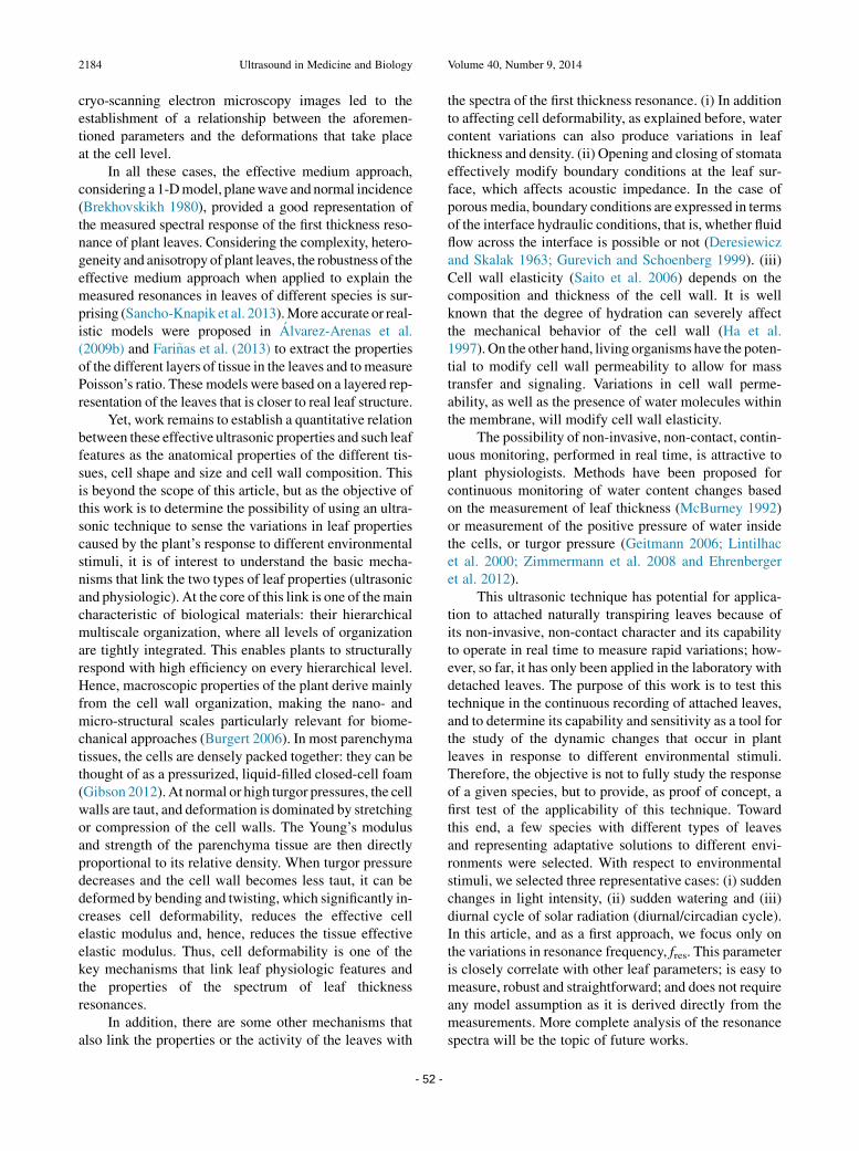
2184 Ultrasound in Medicine and Biology Volume 40, Number 9, 2014

cryo-scanning electron microscopy images led to theestablishment of a relationship between the aforemen-tioned parameters and the deformations that take placeat the cell level.

In all these cases, the effective medium approach,considering a 1-Dmodel, planewave and normal incidence(Brekhovskikh 1980), provided a good representation ofthe measured spectral response of the first thickness reso-nance of plant leaves. Considering the complexity, hetero-geneity and anisotropy of plant leaves, the robustness of theeffective medium approach when applied to explain themeasured resonances in leaves of different species is sur-prising (Sancho-Knapik et al. 2013).More accurate or real-istic models were proposed in �Alvarez-Arenas et al.(2009b) and Fari~nas et al. (2013) to extract the propertiesof the different layers of tissue in the leaves and tomeasurePoisson’s ratio. These models were based on a layered rep-resentation of the leaves that is closer to real leaf structure.

Yet, work remains to establish a quantitative relationbetween these effective ultrasonic properties and such leaffeatures as the anatomical properties of the different tis-sues, cell shape and size and cell wall composition. Thisis beyond the scope of this article, but as the objective ofthis work is to determine the possibility of using an ultra-sonic technique to sense the variations in leaf propertiescaused by the plant’s response to different environmentalstimuli, it is of interest to understand the basic mecha-nisms that link the two types of leaf properties (ultrasonicand physiologic). At the core of this link is one of themaincharacteristic of biological materials: their hierarchicalmultiscale organization, where all levels of organizationare tightly integrated. This enables plants to structurallyrespond with high efficiency on every hierarchical level.Hence, macroscopic properties of the plant derive mainlyfrom the cell wall organization, making the nano- andmicro-structural scales particularly relevant for biome-chanical approaches (Burgert 2006). In most parenchymatissues, the cells are densely packed together: they can bethought of as a pressurized, liquid-filled closed-cell foam(Gibson 2012).At normal or high turgor pressures, the cellwalls are taut, and deformation is dominated by stretchingor compression of the cell walls. The Young’s modulusand strength of the parenchyma tissue are then directlyproportional to its relative density. When turgor pressuredecreases and the cell wall becomes less taut, it can bedeformed by bending and twisting, which significantly in-creases cell deformability, reduces the effective cellelastic modulus and, hence, reduces the tissue effectiveelastic modulus. Thus, cell deformability is one of thekey mechanisms that link leaf physiologic features andthe properties of the spectrum of leaf thicknessresonances.

In addition, there are some other mechanisms thatalso link the properties or the activity of the leaves with

- 52 -

the spectra of the first thickness resonance. (i) In additionto affecting cell deformability, as explained before, watercontent variations can also produce variations in leafthickness and density. (ii) Opening and closing of stomataeffectively modify boundary conditions at the leaf sur-face, which affects acoustic impedance. In the case ofporousmedia, boundary conditions are expressed in termsof the interface hydraulic conditions, that is, whether fluidflow across the interface is possible or not (Deresiewiczand Skalak 1963; Gurevich and Schoenberg 1999). (iii)Cell wall elasticity (Saito et al. 2006) depends on thecomposition and thickness of the cell wall. It is wellknown that the degree of hydration can severely affectthe mechanical behavior of the cell wall (Ha et al.1997).On the other hand, living organisms have the poten-tial to modify cell wall permeability to allow for masstransfer and signaling. Variations in cell wall perme-ability, as well as the presence of water molecules withinthe membrane, will modify cell wall elasticity.

The possibility of non-invasive, non-contact, contin-uous monitoring, performed in real time, is attractive toplant physiologists. Methods have been proposed forcontinuous monitoring of water content changes basedon the measurement of leaf thickness (McBurney 1992)or measurement of the positive pressure of water insidethe cells, or turgor pressure (Geitmann 2006; Lintilhacet al. 2000; Zimmermann et al. 2008 and Ehrenbergeret al. 2012).

This ultrasonic technique has potential for applica-tion to attached naturally transpiring leaves because ofits non-invasive, non-contact character and its capabilityto operate in real time to measure rapid variations; how-ever, so far, it has only been applied in the laboratory withdetached leaves. The purpose of this work is to test thistechnique in the continuous recording of attached leaves,and to determine its capability and sensitivity as a tool forthe study of the dynamic changes that occur in plantleaves in response to different environmental stimuli.Therefore, the objective is not to fully study the responseof a given species, but to provide, as proof of concept, afirst test of the applicability of this technique. Towardthis end, a few species with different types of leavesand representing adaptative solutions to different envi-ronments were selected. With respect to environmentalstimuli, we selected three representative cases: (i) suddenchanges in light intensity, (ii) sudden watering and (iii)diurnal cycle of solar radiation (diurnal/circadian cycle).In this article, and as a first approach, we focus only onthe variations in resonance frequency, fres. This parameteris closely correlate with other leaf parameters; is easy tomeasure, robust and straightforward; and does not requireany model assumption as it is derived directly from themeasurements. More complete analysis of the resonancespectra will be the topic of future works.

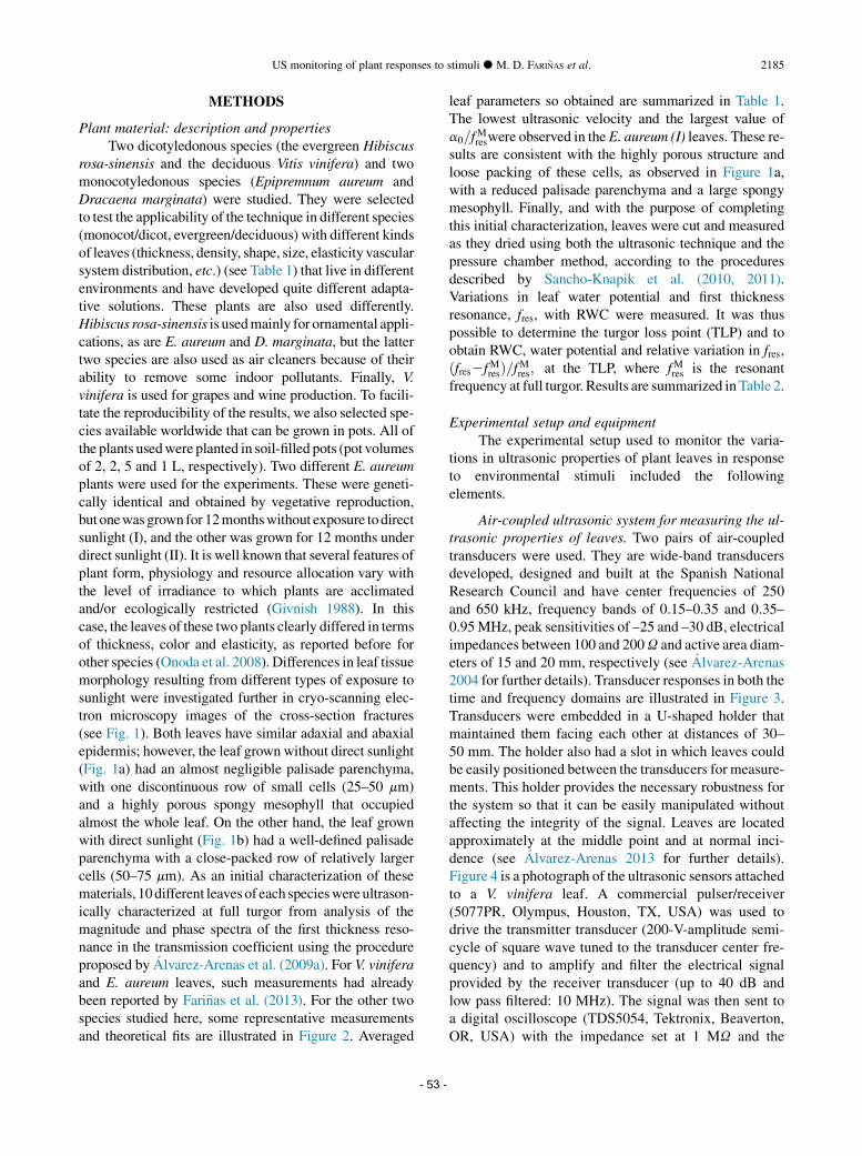
US monitoring of plant responses to stimuli d M. D. FARI~NAS et al. 2185

METHODS

Plant material: description and propertiesTwo dicotyledonous species (the evergreen Hibiscus

rosa-sinensis and the deciduous Vitis vinifera) and twomonocotyledonous species (Epipremnum aureum andDracaena marginata) were studied. They were selectedto test the applicability of the technique in different species(monocot/dicot, evergreen/deciduous) with different kindsof leaves (thickness, density, shape, size, elasticity vascularsystem distribution, etc.) (see Table 1) that live in differentenvironments and have developed quite different adapta-tive solutions. These plants are also used differently.Hibiscus rosa-sinensis is usedmainly for ornamental appli-cations, as are E. aureum and D. marginata, but the lattertwo species are also used as air cleaners because of theirability to remove some indoor pollutants. Finally, V.vinifera is used for grapes and wine production. To facili-tate the reproducibility of the results, we also selected spe-cies available worldwide that can be grown in pots. All ofthe plants usedwere planted in soil-filled pots (pot volumesof 2, 2, 5 and 1 L, respectively). Two different E. aureumplants were used for the experiments. These were geneti-cally identical and obtained by vegetative reproduction,but onewasgrown for 12monthswithout exposure todirectsunlight (I), and the other was grown for 12 months underdirect sunlight (II). It is well known that several features ofplant form, physiology and resource allocation vary withthe level of irradiance to which plants are acclimatedand/or ecologically restricted (Givnish 1988). In thiscase, the leaves of these two plants clearly differed in termsof thickness, color and elasticity, as reported before forother species (Onoda et al. 2008). Differences in leaf tissuemorphology resulting from different types of exposure tosunlight were investigated further in cryo-scanning elec-tron microscopy images of the cross-section fractures(see Fig. 1). Both leaves have similar adaxial and abaxialepidermis; however, the leaf grown without direct sunlight(Fig. 1a) had an almost negligible palisade parenchyma,with one discontinuous row of small cells (25–50 mm)and a highly porous spongy mesophyll that occupiedalmost the whole leaf. On the other hand, the leaf grownwith direct sunlight (Fig. 1b) had a well-defined palisadeparenchyma with a close-packed row of relatively largercells (50–75 mm). As an initial characterization of thesematerials, 10different leavesof each specieswereultrason-ically characterized at full turgor from analysis of themagnitude and phase spectra of the first thickness reso-nance in the transmission coefficient using the procedureproposed by �Alvarez-Arenas et al. (2009a). For V. viniferaand E. aureum leaves, such measurements had alreadybeen reported by Fari~nas et al. (2013). For the other twospecies studied here, some representative measurementsand theoretical fits are illustrated in Figure 2. Averaged

- 53 -

leaf parameters so obtained are summarized in Table 1.The lowest ultrasonic velocity and the largest value ofa0=f

Mreswere observed in the E. aureum (I) leaves. These re-

sults are consistent with the highly porous structure andloose packing of these cells, as observed in Figure 1a,with a reduced palisade parenchyma and a large spongymesophyll. Finally, and with the purpose of completingthis initial characterization, leaves were cut and measuredas they dried using both the ultrasonic technique and thepressure chamber method, according to the proceduresdescribed by Sancho-Knapik et al. (2010, 2011).Variations in leaf water potential and first thicknessresonance, fres, with RWC were measured. It was thuspossible to determine the turgor loss point (TLP) and toobtain RWC, water potential and relative variation in fres,ðfres2fMresÞ=fMres; at the TLP, where fMres is the resonantfrequency at full turgor. Results are summarized in Table 2.

Experimental setup and equipmentThe experimental setup used to monitor the varia-

tions in ultrasonic properties of plant leaves in responseto environmental stimuli included the followingelements.

Air-coupled ultrasonic system for measuring the ul-trasonic properties of leaves. Two pairs of air-coupledtransducers were used. They are wide-band transducersdeveloped, designed and built at the Spanish NationalResearch Council and have center frequencies of 250and 650 kHz, frequency bands of 0.15–0.35 and 0.35–0.95MHz, peak sensitivities of –25 and –30 dB, electricalimpedances between 100 and 200U and active area diam-eters of 15 and 20 mm, respectively (see �Alvarez-Arenas2004 for further details). Transducer responses in both thetime and frequency domains are illustrated in Figure 3.Transducers were embedded in a U-shaped holder thatmaintained them facing each other at distances of 30–50 mm. The holder also had a slot in which leaves couldbe easily positioned between the transducers for measure-ments. This holder provides the necessary robustness forthe system so that it can be easily manipulated withoutaffecting the integrity of the signal. Leaves are locatedapproximately at the middle point and at normal inci-dence (see �Alvarez-Arenas 2013 for further details).Figure 4 is a photograph of the ultrasonic sensors attachedto a V. vinifera leaf. A commercial pulser/receiver(5077PR, Olympus, Houston, TX, USA) was used todrive the transmitter transducer (200-V-amplitude semi-cycle of square wave tuned to the transducer center fre-quency) and to amplify and filter the electrical signalprovided by the receiver transducer (up to 40 dB andlow pass filtered: 10 MHz). The signal was then sent toa digital oscilloscope (TDS5054, Tektronix, Beaverton,OR, USA) with the impedance set at 1 MU and the

Table 1. Averaged leaf properties and their standard variations

SpeciesfMres (kHz)(615%)

Velocity (m/s)(65%)

a0/fMres (Np/(m$kHz)

(67%)Density (kg/m3)

(65%)Thickness (mm)

(615%)C33 (MPa)(67%)

Epipremnum aureum (I) 245 165 3.5 860 330 23Epipremnum aureum (II) 260 200 2.3 915 390 37Hibiscus rosa-sinensis 275 210 2.8 930 380 40Dracaena marginata 645 320 1.7 890 250 92Vitis vinifera 540 215 4.1 760 190 35

2186 Ultrasound in Medicine and Biology Volume 40, Number 9, 2014

bandwidth set at 20 MHz and averaged (between 80 and120 samples). Samples were digitized at 2 and 5MS/s, formeasurements in the 250- and 650-kHz bands, respec-tively, and at 8 bit (amplitude). The result was then trans-ferred to the oscilloscope PC for further signal analysis.First, a rectangular time window was applied to the trans-mitted waveform to filter out the reverberations within theair cavities. The signal was padded with zeroes up to 4Kto increase frequency resolution, and then the Fouriertransform was extracted using the fast Fourier Transform(FFT) algorithm. Real and imaginary parts of the FFTareused to compute the magnitude and phase spectra of thetransmitted signal. Further calculations to obtain the fre-quency location of the maximum transmission (resonantfrequency) or the Q-factor of the resonance were per-formed in MATLAB (The MathWorks, Natick, MA,USA) (see Sancho-Knapik et al. 2012). Given these con-ditions for the analogue-to-digital conversion, the preci-sion in the determination of the resonant frequency isdetermined by the discretization in frequency, which is488 and 1220 Hz in the 250- and 650-kHz frequencybands, respectively. Hence, precision in the determinationof the relative variation in the resonant frequency is in therange 0.3%–0.8%. Repeatability of the measurement ofthe resonant frequency is ,0.8%.

System of conventional sensors to monitor varia-tions in plant environment. Four different sensors were

Fig. 1. Cryo-scanning electron microscopy (SEM) images of thAdaxial epidermis. (2) Palisade parenchyma. (3) Spongy mesop

light (Epipremnum aureum I). (b) Grown with direct su

- 54 -

employed to measure air and soil temperature, soil ten-sion and light intensity. For soil tension measurements,a Watermark 200SS-V sensor (Irrometer, Riverside,CA, USA) was used. It consists of a pair of highlycorrosion-resistant electrodes that are embedded withina granular matrix. A current was applied to obtain a resis-tance value. The sensor correlated the resistance to soilwater tension. With respect to light intensity, a photosyn-thetically active radiation sensor was used. As photosyn-thesis is driven by the number of photons in this band, theintensity was measured in number of photons (in mol) persecond and per unit surface (mmol m22 s21). The photo-synthetic photon flux (PPF) sensor (SQ-200-5, ApogeeInstruments, Logan, UT, USA) was used for this pur-pose. According to the manufacturer, its sensitivity is2.0 mV per mmol m22 s21 with a calibration factor of0.5 mmolm22 s21 per mV, andmeasurement repeatabilityis ,1%. In all the measurements reported in this article,the source of light was the sun. All of these sensorswere connected to a data logger (FieldLogger FL,NOVUS, Porto Alegre, Rio Grande do Sul, Brazil).This is a microprocessor-based data acquisition andrecorder that can handle analogue inputs and can operateas a remote terminal unit linked to a PC for on-linerecording or as a stand-alone data logger with real-timeclock and graph capabilities. In this case, it was used asa stand-alone data logger. It has eight channels that accept

e cross sections of two leaves of Epipremnum aureum. (1)hyl. (4) Abaxial epidermis. (a) Grown without direct sun-nlight (Epipremnum aureum II). Bar 5 200 mm.

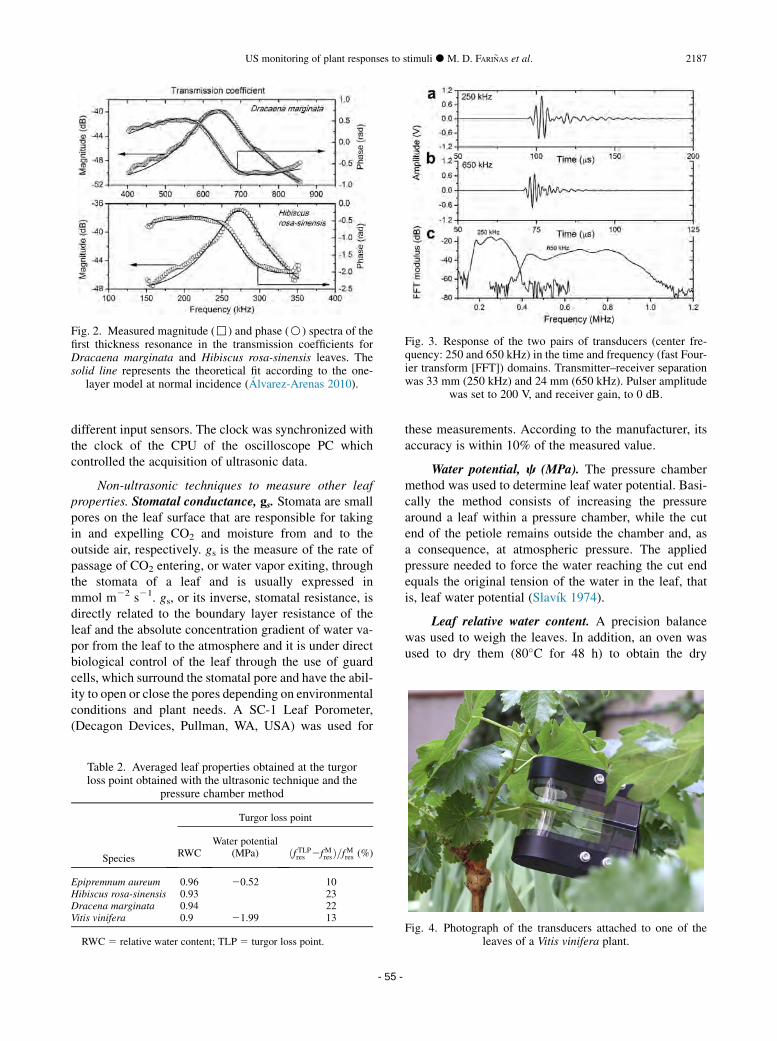
Fig. 2. Measured magnitude (,) and phase (B) spectra of thefirst thickness resonance in the transmission coefficients forDracaena marginata and Hibiscus rosa-sinensis leaves. Thesolid line represents the theoretical fit according to the one-

layer model at normal incidence (�Alvarez-Arenas 2010).

Fig. 3. Response of the two pairs of transducers (center fre-quency: 250 and 650 kHz) in the time and frequency (fast Four-ier transform [FFT]) domains. Transmitter–receiver separationwas 33 mm (250 kHz) and 24 mm (650 kHz). Pulser amplitude

was set to 200 V, and receiver gain, to 0 dB.

US monitoring of plant responses to stimuli d M. D. FARI~NAS et al. 2187

different input sensors. The clock was synchronized withthe clock of the CPU of the oscilloscope PC whichcontrolled the acquisition of ultrasonic data.

Non-ultrasonic techniques to measure other leafproperties. Stomatal conductance, gs. Stomata are smallpores on the leaf surface that are responsible for takingin and expelling CO2 and moisture from and to theoutside air, respectively. gs is the measure of the rate ofpassage of CO2 entering, or water vapor exiting, throughthe stomata of a leaf and is usually expressed inmmol m22 s21. gs, or its inverse, stomatal resistance, isdirectly related to the boundary layer resistance of theleaf and the absolute concentration gradient of water va-por from the leaf to the atmosphere and it is under directbiological control of the leaf through the use of guardcells, which surround the stomatal pore and have the abil-ity to open or close the pores depending on environmentalconditions and plant needs. A SC-1 Leaf Porometer,(Decagon Devices, Pullman, WA, USA) was used for

Table 2. Averaged leaf properties obtained at the turgorloss point obtained with the ultrasonic technique and the

pressure chamber method

Species

Turgor loss point

RWCWater potential

(MPa) ðf TLPres 2fMresÞ=fMres (%)

Epipremnum aureum 0.96 20.52 10Hibiscus rosa-sinensis 0.93 23Dracena marginata 0.94 22Vitis vinifera 0.9 21.99 13

RWC 5 relative water content; TLP 5 turgor loss point.

- 55 -

these measurements. According to the manufacturer, itsaccuracy is within 10% of the measured value.

Water potential, c (MPa). The pressure chambermethod was used to determine leaf water potential. Basi-cally the method consists of increasing the pressurearound a leaf within a pressure chamber, while the cutend of the petiole remains outside the chamber and, asa consequence, at atmospheric pressure. The appliedpressure needed to force the water reaching the cut endequals the original tension of the water in the leaf, thatis, leaf water potential (Slav�ık 1974).

Leaf relative water content. A precision balancewas used to weigh the leaves. In addition, an oven wasused to dry them (80�C for 48 h) to obtain the dry

Fig. 4. Photograph of the transducers attached to one of theleaves of a Vitis vinifera plant.

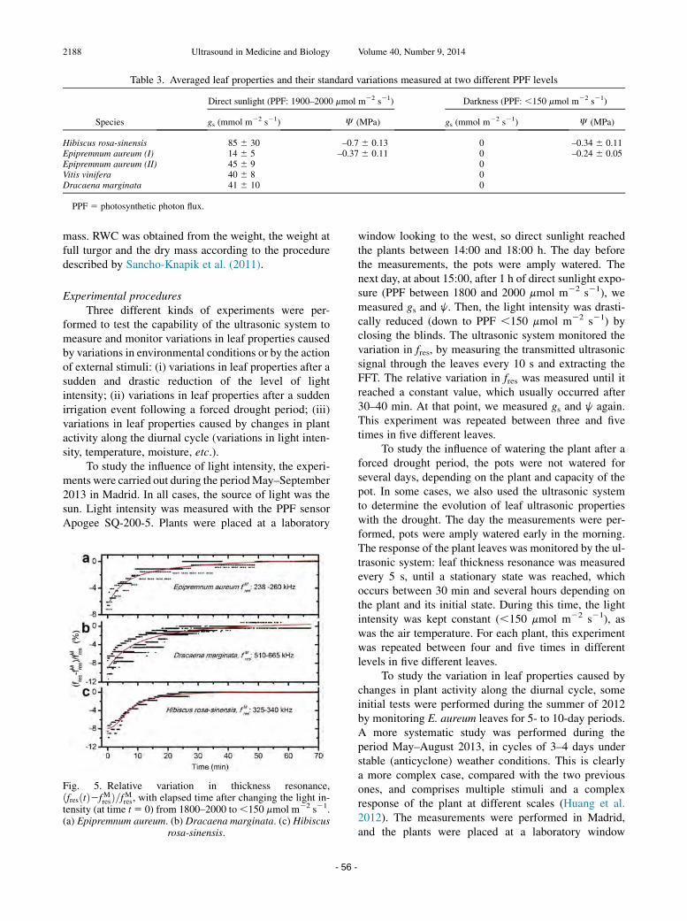
Table 3. Averaged leaf properties and their standard variations measured at two different PPF levels

Species

Direct sunlight (PPF: 1900–2000 mmol m22 s21) Darkness (PPF: ,150 mmol m22 s21)

gs (mmol m22 s21) J (MPa) gs (mmol m22 s21) J (MPa)

Hibiscus rosa-sinensis 85 6 30 –0.7 6 0.13 0 –0.34 6 0.11Epipremnum aureum (I) 14 6 5 –0.37 6 0.11 0 –0.24 6 0.05Epipremnum aureum (II) 45 6 9 0Vitis vinifera 40 6 8 0Dracaena marginata 41 6 10 0

PPF 5 photosynthetic photon flux.

2188 Ultrasound in Medicine and Biology Volume 40, Number 9, 2014

mass. RWC was obtained from the weight, the weight atfull turgor and the dry mass according to the proceduredescribed by Sancho-Knapik et al. (2011).

Experimental proceduresThree different kinds of experiments were per-

formed to test the capability of the ultrasonic system tomeasure and monitor variations in leaf properties causedby variations in environmental conditions or by the actionof external stimuli: (i) variations in leaf properties after asudden and drastic reduction of the level of lightintensity; (ii) variations in leaf properties after a suddenirrigation event following a forced drought period; (iii)variations in leaf properties caused by changes in plantactivity along the diurnal cycle (variations in light inten-sity, temperature, moisture, etc.).

To study the influence of light intensity, the experi-ments were carried out during the periodMay–September2013 in Madrid. In all cases, the source of light was thesun. Light intensity was measured with the PPF sensorApogee SQ-200-5. Plants were placed at a laboratory

Fig. 5. Relative variation in thickness resonance,ðfresðtÞ2fMresÞ=fMres, with elapsed time after changing the light in-tensity (at time t5 0) from 1800–2000 to,150 mmol m22 s21.(a) Epipremnum aureum. (b) Dracaena marginata. (c) Hibiscus

rosa-sinensis.

- 56 -

window looking to the west, so direct sunlight reachedthe plants between 14:00 and 18:00 h. The day beforethe measurements, the pots were amply watered. Thenext day, at about 15:00, after 1 h of direct sunlight expo-sure (PPF between 1800 and 2000 mmol m22 s21), wemeasured gs and j. Then, the light intensity was drasti-cally reduced (down to PPF ,150 mmol m22 s21) byclosing the blinds. The ultrasonic system monitored thevariation in fres, by measuring the transmitted ultrasonicsignal through the leaves every 10 s and extracting theFFT. The relative variation in fres was measured until itreached a constant value, which usually occurred after30–40 min. At that point, we measured gs and j again.This experiment was repeated between three and fivetimes in five different leaves.

To study the influence of watering the plant after aforced drought period, the pots were not watered forseveral days, depending on the plant and capacity of thepot. In some cases, we also used the ultrasonic systemto determine the evolution of leaf ultrasonic propertieswith the drought. The day the measurements were per-formed, pots were amply watered early in the morning.The response of the plant leaves was monitored by the ul-trasonic system: leaf thickness resonance was measuredevery 5 s, until a stationary state was reached, whichoccurs between 30 min and several hours depending onthe plant and its initial state. During this time, the lightintensity was kept constant (,150 mmol m22 s21), aswas the air temperature. For each plant, this experimentwas repeated between four and five times in differentlevels in five different leaves.

To study the variation in leaf properties caused bychanges in plant activity along the diurnal cycle, someinitial tests were performed during the summer of 2012by monitoring E. aureum leaves for 5- to 10-day periods.A more systematic study was performed during theperiod May–August 2013, in cycles of 3–4 days understable (anticyclone) weather conditions. This is clearlya more complex case, compared with the two previousones, and comprises multiple stimuli and a complexresponse of the plant at different scales (Huang et al.2012). The measurements were performed in Madrid,and the plants were placed at a laboratory window

Fig. 6. Relative variation in thickness resonance, ðfresðtÞ2fMresÞ=fMres, with the elapsed time after the plant is watered (attime 5 0). (a) Epipremnum aureum. (b) Dracaena marginata. (c) Hibiscus rosa-sinensis. (d) Vitis vinifera.

US monitoring of plant responses to stimuli d M. D. FARI~NAS et al. 2189

looking to the west, so direct sunlight reached the plantsat intervals between 14:00 and 18:00 h. Air and soiltemperature, soil tension and photosynthetically activeradiation were measured and stored in the autonomousdata logger (Novus Field Logger) every 10 min. Ultra-sonic measurements were controlled with the oscillo-scope PC and taken every 10 min as well. The nightbefore the monitoring started, the pots were amply wa-tered. The next day, we started measurements early inthe morning, and no additional water was supplied duringthe 3–4 days of monitoring. This procedure was repeatedbetween three and five times for each plant in fivedifferent leaves.

Fig. 7. Evolution of the thickness resonant frequency of an Epi-premnum aureum (I) leaf over 4 days. Photosynthetic photonflux (PPF) and ambient temperature measurements are also

shown.

RESULTS AND DISCUSSION

In general, it is observed that the frequency of thefirst-order thickness resonance of plant leaves changeswhen the plant is subjected to the different stimuli studiedhere. The actual behavior depends on the type of stimuli,the specific properties of the leaves of this species, theenvironmental conditions under which the plant wasgrown and the actual state of the leaf and the plant itself.The species studied here were chosen to reflect differentplant types (monocot/dicot, evergreen/deciduous) havingleaves with different properties (thickness, density, shape,size, elasticity vascular system distribution, tissue physi-ology. etc.) and found in different environments in whichthey have developed quite different adaptative solutions.

- 57 -

Fig. 8. Evolution of the thickness resonant frequency of an Epi-premnum aureum (II) leaf over 3.5 days. Photosynthetic photonflux (PPF) and ambient temperature measurements are also

shown.

Fig. 9. Evolution of the thickness resonant frequency of aHibis-cus rosa-sinensis leaf over 4 days. Photosynthetic photon flux(PPF) and ambient temperature measurements are also shown.

2190 Ultrasound in Medicine and Biology Volume 40, Number 9, 2014

It is expected that the technique can be equally applied toany other species in which thickness resonances of theleaves can be measured, though the actual behavior willdepend on the specific features of the species and theplant under study.

Ultrasonic monitoring of plant response to lightintensity reduction

Variations in gs and j with light intensity reductionare summarized in Table 3, Figure 5 illustrates the relativevariation in resonant frequency with elapsed time,ðfresðtÞ--fMresÞ=fMres; where fMres is the maximum value of theleaf resonant frequency that is obtained when the plantis in darkness ðfMres 5 f darkres Þ, and t 5 0 corresponds to thetime when light intensity was reduced. Data in Table 3indicate that the reduction in light intensity induces sto-matal closure and an increase in j. This decrease in tran-spiration, mediated by stomatal closure, shifts the balancebetween water supply and water evaporation and in-creases leaf RWC and turgor pressure. Concerning leaf ul-trasonic properties, Figure 5 illustrates that fres increasesin all cases, and the maximum value is achieved whenthe plant is placed in the dark. As explained before, this

- 58 -

shift of fres toward higher values is produced by an in-crease in the ultrasound velocity in the leaf, which is theresult of a stiffening of the tissues caused by the increasein turgor pressure. The variation in fres with time can beestimated by the sigmoid function (also illustrated inFig. 5).

fresðtÞ2f darkres

f darkres

5A21

11ðt=t0Þp

where t is the elapsed time, t0 is the time at which thepoint of inflection of the sigmoid is located, p determineshow fast is the sigmoid transition from the lower to theupper bounds and A5 f lightres =f darkres , where f lightres is the mini-mum value of the resonant frequency (measured at t5 0).A sigmoid is selected because this law is well fitted todescribe a transition between two states (as is the casehere) and provides a quantification of the variation rateor the location of the point of inflection.

Ultrasonic monitoring of plant response to wateringVariation in ðfresðtÞ2fMresÞ=fMres after a sudden irrigation

following a forced drought period is illustrated in Figure 6.Unlike the previous experiment, this variation is nowaffected by two different mechanisms. On the one hand,

Fig. 10. Evolution of the thickness resonant frequency of aDracaena marginata leaf over 3.5 days. Photosynthetic photonflux(PPF)andambient temperaturemeasurementsarealsoshown.

Fig. 11. Evolution of the thickness resonant frequency of a Vitisvinifera leaf over 3.5 days. Photosynthetic photon flux (PPF)

and ambient temperature measurements are also shown.

US monitoring of plant responses to stimuli d M. D. FARI~NAS et al. 2191

the total ranges of variation, ðfresðt5 0Þ2fMresÞ=fMres, isdetermined mainly by leaf tissue properties; in particular,by how much the cell wall tautness can change with leafRWC. On the other hand, the kinetics of the process isdetermined by the velocity of the water transport fromthe soil to the leaves. This depends on many factors suchas the permeability of the cell wall, the plant vascular sys-tem, the distance between the leaf and the roots, the integ-rity of the vascular system and the transport mechanismsin the actual water path that connects the leaf and the roots.In all cases, a shift in fres toward higher frequencies isobserved. This is the expected result considering that theRWC of the leaves and, consequently, the tautness of thecell walls are expected to increase after watering. Cleardifferences between species can be observed in the rangeand rate of variation of fres. In addition, if wecompareðfresðt5 0Þ2fMresÞ=fMres in Figure 6 with the valueof ðf TLPres 2fMresÞ=fMres (measured at TLP, see Table 2), weobserve two different types of behaviors. For E. aureumand D. marginata, ðfresðt5 0Þ2fMresÞ=fMres is considerablysmaller than ðf TLPres 2fMresÞ=fMres, whereas for H. rosa-sinene-sis andV. vinifera, bothmagnitudes are similar. The expla-nation of these differences may well correspond to thedifferent plant strategies used to copewith water shortage:

- 59 -

Although some species can reduce leaf RWC close to thevalue for TLP, some others, with a more ‘‘conservativestrategy,’’ limit the water loss well before reaching TLP.More data are required to draw any conclusion in thissense, but the present study reveals the potential of thetechnique for this application.

Unlike previous experiments, and according to thetwo different mechanisms that determine the kinetics ofthis process (cell wall elasticity and vascular system),large variations between species and between differentleaves of the same species in the time needed to reachfMres are observed. Two different factors determine thesevariations. The first corresponds to variations in theinitial point (i.e., differences in how dry the plant wasat t 5 0). The second corresponds to variation in thevascular system caused by the possible appearance ofdifferent levels of embolisms produced by the forceddrought that can limit, at least initially, the capacity totransport water and/or the velocity with which the wateris transported.

Ultrasonic monitoring of variations in the plant alongthe diurnal cycle

Measured variations in leaf properties (resonantfrequency, ambient temperature and light intensity)

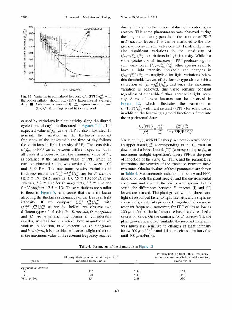
Fig. 12. Variation in normalized frequency, fresðPPFÞ=fMres, withthe photosynthetic photon flux (PPF). Experimental averageddata: -, Epipremnum aureum (I); O, Epipremnum aureum

(II); B, Vitis vinifera and fit to a sigmoid.

2192 Ultrasound in Medicine and Biology Volume 40, Number 9, 2014

caused by variations in plant activity along the diurnalcycle (time of day) are illustrated in Figures 7–11. Theexpected value of fres at the TLP is also illustrated. Ingeneral, the variation in the thickness resonantfrequency of the leaves with the time of day followsthe variations in light intensity (PPF). The sensitivityof fres to PPF varies between different species, but inall cases it is observed that the minimum value of fresis obtained at the maximum value of PPF, which, inour experimental setup, was achieved between 1:00and 6:00 PM. The maximum relative variations inthickness resonance ðfmin

res 2fMresÞ=fMres are for E. aureum(I), 5 6 1%; for E. aureum (II), 7.5 6 1%; for H. rosa-sinensis, 5.2 6 1%; for D. marginata, 8.5 6 1%; andfor V. vinifera, 12.5 6 1%. These variations are similarto those in Figure 5, so it seems that the main factoraffecting the thickness resonances of the leaves is lightintensity. If we compare ðfmin

res 2fMresÞ=fMres withðf TLPres 2fMresÞ=fMres as we did before, we observe twodifferent types of behavior. For E. aureum,D. marginataand H. rosa-sinenesis, the former is considerablysmaller, whereas for V. vinifera, both magnitudes aresimilar. In addition, in E. aureum (I), D. marginataand V. vinifera, it is possible to observe a slight reductionin the maximum value of the resonant frequency reached

Table 4. Parameters of the s

SpeciesPhotosynthetic photon flux at the point of

inflection (mmol/m2$s)

Epipremnum aureum(I) 116(II) 221

Vitis vinifera 154

- 60 -

during the night as the number of days of monitoring in-creases. This same phenomenon was observed duringthe longer monitoring periods in the summer of 2012in E. aureum leaves. This can be attributed to the pro-gressive decay in soil water content. Finally, there arealso significant variations in the sensitivity ofðfres2fMresÞ=fMres to variations in light intensity. While forsome species a small increase in PPF produces signifi-cant variation in ðfres2fMresÞ=fMres, other species seem tohave a light intensity threshold and changes inðfres2fMresÞ=fMres are negligible for light variations belowthis threshold. Leaves of the former type also exhibit asaturation of ðfres2fMresÞ=fMres, and once the maximumvariation is achieved, this value remains constantregardless of a possible further increase in light inten-sity. Some of these features can be observed inFigure 12, which illustrates the variation infresðPPFÞ=fMres with light intensity (PPF) for some cases;in addition the following sigmoid function is fitted intothe experimental data:

fresðPPFÞfMres

5fminres

fMres1

12fminres

�fMres

11ðPPF=PPF0Þp

Variation in fres with PPF takes place between two bonds:an upper bound, fMres (corresponding to the fres value atdawn), and a lower bound, fmin

res (corresponding to fres atmaximum sunlight exposition), where PPF0 is the pointof inflection of the curve fres (PPF), and the parameter pdetermines the velocity of the transition between thesetwo states. Obtained values of these parameters are shownin Table 4. Measurements indicate that both p and PPF0depend on both the plant species and the environmentalconditions under which the leaves were grown. In thissense, the differences between E. aureum (I) and (II)leaves are marked. The plant grown without direct sun-light (I) responded faster to light intensity, and a slight in-crease in light intensity produced a significant decrease inresonant frequency; moreover, for PPF values as low as200 mmol/m2$s, the leaf response has already reached asaturation value. On the contrary, for E. aureum (II), theplant grown under direct sunlight, the resonant frequencywas much less sensitive to changes in light intensitybelow 200 mmol/m2$s and did not reach a saturation valueuntil 800 mmol/m2$s.

igmoid fit in Figure 12

p

Photosynthetic photon flux at frequencyresponse saturation (99% of total variation)

(mmol/m2$s)

2.54 1655.41 4462.89 390

US monitoring of plant responses to stimuli d M. D. FARI~NAS et al. 2193

CONCLUSIONS

The work reported here indicates that the air-coupled and wide-band ultrasonic technique describedis able to detect, in a non-destructive, non-invasive,non-contact, rapid manner, variations in leaf thicknessresonances caused by the response of the plant todifferent environmental stimuli. Mechanisms that linkmodification of the main features of leaf thickness reso-nances with the variation in leaf parameters and plant ac-tivity have been proposed.

Decreasing light intensity (from 2000 to150 mmol m22 s21) produces an increase in the leaf thick-ness resonant frequency (between 8% and 12%, depend-ing on the species). This is explained by the reduction inplant transpiration, the closure of stomata and theconcomitant shift in water equilibrium in the leaves. Wa-tering the plant after a period of forced drought producesan increase in the thickness resonant frequency (5%–30%depending on the species and the plant) which is attrib-uted to the increase in cell turgor pressure resultingfrom the increase in the RWC of the leaves. The kineticsof this phenomenon depends on the water transport chan-nels between the soil and the leaves, and the time spanvaries between 10 and 400 min. These variations can beattributed to differences in the length, efficiency or integ-rity of these channels. Observed variations in the resonantfrequency along the diurnal cycle (4%–10%) largelyreflect the variations in light intensity. In addition, the ki-netics of this response and the presence of saturationlevels seem to depend on the mechanisms these plantsuse to adapt to the sunlight intensity available.

Finally, we observed that compared with the varia-tion at the TLP, ðf TLPres 2fMresÞ=fMres, the variation inðfres2fMresÞ=fMres differs significantly depending on the stim-uli and the species. Although in some cases we observedfluctuations in the resonant frequency much smaller thanthe variation observed at the TLP, in other cases, thesevariations are similar. This may reflect differences be-tween different species and different individuals indealing with the environmental stimuli. Clearly, furtherwork and experimental evidence are needed, but these re-sults reveal the potential of this technique as a tool thatcan provide meaningful data.

Acknowledgments—Authors acknowledge funding from the SpanishMinistry for Economy and Competitivity, through Project DPI2011-22438, and a Botin Foundation grant given to M. D. Fari~nas.

REFERENCES

Akseli I, Dey D, Cetinkaya C. Mechanical property characterization ofbilayered tablets using nondestructive air-coupled acoustics. AAPSPharmSciTech 2010;11:90–102.

�Alvarez-Arenas TEG, Montero FR, Moner-Girona M, Roig A,Molins E. Viscoelasticity of silica aerogels at ultrasonic frequencies.Appl Phys Lett 2002;81:1198–1200.

- 61 -

�Alvarez-Arenas TEG. Acoustic impedance matching of piezoelectrictransducers to the air. IEEE Trans Ultrason Ferroelectr Freq Control2004;51:624–633.

�Alvarez-Arenas TEG. Simultaneous determination of the ultrasound ve-locity and the thickness of solid plates from the analysis of thicknessresonances using air-coupled ultrasound. Ultrasonics 2010;50:104–109.

�Alvarez-Arenas TEG. Air-coupled piezoelectric transducers with activepolypropylene foam matching layers. Sensors 2013;13:5996–6013.

�Alvarez-Arenas TEG, Cal�as H, Cuello JE, Fern�andez AR, Mu~noz M.Noncontact ultrasonic spectroscopy applied to the study of polypro-pylene ferroelectrets. J Appl Phys 2010;108:074110.

�Alvarez-Arenas TEG, D�ıez L. Novel impedance matching materials andstrategies for air-coupled piezoelectric transducers. In: Proceedings,2013 IEEE Sensors, Baltimore, Maryland, USA, 3–6 November2013. New York: IEEE; 2013.

�Alvarez-Arenas TEG, Sancho-Knapik D, Peguero-Pina JJ,Gil-Pelegrin E. Noncontact and noninvasive study of plant leaves us-ing air-coupled ultrasounds. Appl Phys Lett 2009a;95:193702.

�Alvarez-Arenas TEG, Sancho-Knapik D, Peguero-Pina JJ,Gil-Pelegr�ın E. Determination of plant leaves water status usingair-coupled ultrasounds. In: Proceedings, 2009 IEEE InternationalUltrasonics Symposium, Rome, Italy, 20–23 September 2009.New York: IEEE; 2009b. p. 771–774.

�Alvarez-Arenas TEG, Shrout TR, Zhang SJ, Lee HJ. Air-coupled trans-ducers based on 1–3 connectivity single crystal transducers. In: Pro-ceedings, 2012 IEEE International Ultrasonics Symposium,Dresden, Germany, 7–10 October 2012. New York: IEEE; 2012. p.2230–2233.

Brekhovskikh LM. Waves in layered media. 2nd ed. New York: Aca-demic Press; 1980.

Burgert I. Exploring the micromechanical design of plant cell walls. AmJ Bot 2006;93:1391–1401.

Deresiewicz H, Skalak R. On uniqueness in dynamic poroelasticity. BullSeism Soc Am 1963;53:783–788.

Ealo JL, Camacho J, Fritsch C, Seco F, Roa J. A fabrication procedure forairborne ultrasonic phased arrays based on cellular electromechanicalfilm. In: Proceedings, 2008 IEEE Ultrasonics Symposium, Beijing,China, 2–5 November 2008. New York: IEEE; 2008. p. 891–894.

Ehrenberger W, R€uger S, Rodr�ıguez-Dom�ınguez CM, D�ıaz-Espejo A,Fern�andez JE, Moreno J, Zimmermann D, Sukhorukov VL,Zimmermann U. Leaf patch clamp pressure probe measurementson olive leaves in a nearly turgorless state. Plant Biol 2012;14:666–674.

Fari~nasMD, Sancho-Knapik D, Peguero-Pina JJ, Gil-Pelegrin E, GomezAlvarez-Arenas TEG. Shear waves in vegetal tissues at ultrasonicfrequencies. Appl Phys Lett 2013;102:103702.

Fukuhara M. Acoustic characteristics of botanical leaves using ultra-sonic transmission waves. Plant Sci 2002;162:521–528.

Geitmann A. Experimental approaches used to quantify physical param-eters at cellular and subcellular levels.AmJBot 2006;93:1380–1390.

Gibson L. The hierarchical structure and mechanics of plant materials.J R Soc Interface 2012;9:2749–2766.

Givnish TJ. Adaptation to sun and shade: A whole-plant perspective.Aust J Plant Physiol 1988;15:63–92.

Gurevich B, Schoenberg M. Interface conditions for Biot’s equations ofporoelasticity. J Acoust Soc Am 1999;105:2585–2589.

Ha MA, Apperley DC, Jarvis MC. Molecular rigidity in dry and hydrat-ed onion cell walls. Plant Physiol 1997;115:593–598.

Haller MI, Edward L, Khuri-Yakub BT. 1–3 Composites for ultrasonicair transducers. In: . New York: IEEE; 1992. p. 937–939.

Hayward G, Gachagan A. An evaluation of 1–3 connectivity compositetransducers for air-coupled ultrasonic applications. JAcoust Soc Am1996;99:2148–2157.

Hsu DK. Nondestructive testing using air-borne ultrasound. Ultrasonics2006;44:1019–1024.

Huang W, P�erez-Garc�ıa P, Pokhilko A, Millar AJ, Antoshechkin I,Riechmann JL, Mas P. Mapping the core of the Arabidopsis circa-dian clock defines the network structure of the oscillator. Science2012;336:75–79.

Hutchins DA, Schindel DW, Bashford AG, Wright WMD. Advances inultrasonic electrostatic transduction. Ultrasonics 1998;36:1–6.

2194 Ultrasound in Medicine and Biology Volume 40, Number 9, 2014

Hutchins DA, Wright WM, Schindel DW. Ultrasonic measurements inpolymeric materials using air-coupled capacitance transducers.J Acoust Soc Am 1994;96:1634–1642.

Kelly SP, Hayward G, �Alvarez-Arenas TEG. Characterization andassessment of an integrated matching layer for air-coupled ultra-sonic applications. IEEE Trans Ultrason Ferroelectr Freq Control2004;51:1314–1323.

Lintilhac PM,Wei C, Tanguay JJ, Outwater JO. Ball tonometry: A rapid,non-destructive method for measuring cell turgor pressure in thin-walled plant cells. J Plant Growth Regul 2000;19:90–97.

Livings RA, Dayal V, Barnard DJ, Hsu DK. Flaw investigation in amulti-layered, multi-material composite: Using air-coupled ultra-sonic resonance imaging. AIP Conf Proc 2012;1430:1176–1183.

McBurney T. The relationship between leaf thickness and plant waterpotential. J Exp Bot 1992;43:327–335.

Onoda Y, Schievig F, Anten NPR. Effects of light and nutrient availabil-ity on leaf mechanical properties of Plantago major: A conceptualapproach. Ann Bot 2008;101:727–736.

Saito T, Soga K, Hoson T, Terashima I. The bulk elastic modulus and thereversible properties of cell walls in developing Quercus leaves.Plant Cell Physiol 2006;47:715–725.

Sancho-Knapik D, �Alvarez-Arenas TEG, Peguero-Pina JJ, Fern�andez V,Gil-Pelegr�ın E. Relationship between ultrasonic properties andstructural changes in the mesophyll during leaf dehydration. J ExpBot 2011;62:3637–3645.

Sancho-Knapik D, �Alvarez-Arenas TEG, Peguero-Pina JJ,Gil-Pelegr�ın E. Air-coupled broadband ultrasonic spectroscopy asa new non-invasive and non-contact method for the determinationof leaf water status. J Exp Bot 2010;61:1385–1391.

Sancho-Knapik D, Cal�as H, Peguero-Pina JJ, Ramos Fern�andez A,Gil-Pelegr�ın E, �Alvarez-Arenas TEG. Air-coupled ultrasonic reso-nant spectroscopy for the study of the relationship between plant

- 62 -

leaves’ elasticity and their water content. IEEE Trans Ultrason Fer-roelectr Freq Control 2012;59:319–325.

Sancho-Knapik D, Peguero-Pina JJ, Fari~nas MD, �Alvarez-Arenas TEG,Gil-Pelegr�ın E. Ultrasonic spectroscopy allows a rapid determina-tion of the relative water content at the turgor loss point: a compar-ison with pressure-volume curves in 13 woody species. Tree Physiol2013;33:695–700.

Schindel DW, Hutchins DA. Through-thickness characterization ofsolids by wideband air-coupled ultrasound. Ultrasonics 1995;33:11–17.

Schindel DW, Hutchins DA, Zou L, Sayer M. The design and char-acterization of micromachined air-coupled capacitance trans-ducers. IEEE Trans Ultrason Ferroelectr Freq Control 1995;42:42–50.

Schindel DW, Hutchins DA, Grandia WA. Capacitive and piezoelectricair-coupled transducers for resonant ultrasonic inspection. Ultra-sonics 1996;34:621–627.

Scholander PF, Bradstreet ED, Hemmingsen EA, Hammel HT. Sap pres-sure in vascular plants negative hydrostatic pressure can bemeasured in plants. Science 1965;148:339–346.

Slav�ık B. Methods of studying plant water relations. Berlin: Springer;1974.

Wilson PS, Dunton KH. Laboratory investigation of the acousticresponse of seagrass tissue in the frequency band 0.5–2.5 kHz.J Acoust Soc Am 2009;125:1951–1959.

Yano T, Tone M, Fukumoto A. Range finding and surface characteriza-tion using high-frequency air transducers. IEEE Trans Ultrason Fer-roelectr Freq Control 1987;34:232–236.

Zimmermann D, Reuss R, Westhoff M, Geßner P, Bauer W, Bamberg E,Bentrup FW, Zimmermann U. A novel, noninvasive, online-monitoring, versatile and easy plant-based probe for measuringleaf water status. J Exp Bot 2008;59:3157–3167.

Physics Procedia 63 ( 2015 ) 91 – 96

Available online at www.sciencedirect.com

1875-3892 © 2015 The Authors. Published by Elsevier B.V. This is an open access article under the CC BY-NC-ND license (http://creativecommons.org/licenses/by-nc-nd/4.0/).Peer-review under responsibility of the Ultrasonic Industry Associationdoi: 10.1016/j.phpro.2015.03.015

ScienceDirect

43rd Annual Symposium of the Ultrasonic Industry Association, UIA Symposium 2014

Monitoring of plant light/dark cycles using air-coupled ultrasonic spectroscopy

M.D. Fariñas a, D. Sancho-Knapik b, J. Peguero-Pina b, E. Gil-Pelegrín b and T.E.G.Álvarez-Arenas a

aSensors and Ultrasonic Technologies Department, Information and Physics Technolgies Institute (ITEFI), Spanish National Research Council (CSIC), Serrano 144, 28006, Madrid, Spain

bAgrifood Research and Technology Centre of Aragon (CITA). Avd. Montañana 930, 50059 Zaragoza, Spain.

Abstract

This work presents the application of a technique based on the excitation, sensing and spectral analysis of leaves thickness resonances using air-coupled and wide-band ultrasound to monitor variations in leaves properties due to the plant response along light/dark cycles. The main features of these resonances are determined by the tautness of the cells walls in such a way that small modifications produced by variations in the transpiration rate, stomata aperture or water potential have a direct effect on the thickness resonances that can be measured in a completely non-invasive and contactless way. Results show that it is possible to monitor leaves changes due to variations in light intensity along the diurnal cycle, moreover, the technique reveals differences in the leaf response for different species and also within the same species but for specimens grown under different conditions that present different cell structures at the tissue level.

PACS: 43.20+g; 43.80 +p; 45.35 +d;

© 2014 The Authors. Published by Elsevier B.V.Peer-review under responsibility of the Ultrasonic Industry Association.

Keywords: Plant leaves; Water content; drought stress; circadian rythms; air-coupled; ultrasoni spectroscopy; monitoring;

© 2015 The Authors. Published by Elsevier B.V. This is an open access article under the CC BY-NC-ND license (http://creativecommons.org/licenses/by-nc-nd/4.0/).Peer-review under responsibility of the Ultrasonic Industry Association

- 63 -

92 M.D. Fariñas et al. / Physics Procedia 63 ( 2015 ) 91 – 96

1. Introduction

Improvements in air-coupled transducers have boosted the applications of air-coupled ultrasound to materialscharacterization and to non-destructive testing technique; in particular, the use of spectral analysis of thickness resonances in solid plates (Yano et al., 1987; Haller et al., 1992; Schindel and Hutchins 1995; Álvarez-Arenas et al., 2002; Álvarez-Arenas 2004; Álvarez-Arenas et al., 2010; Álvarez-Arenas et al., 2012; Álvarez-Arenas 2013; Álvarez-Arenas and Díez 2013). Conventional ultrasonic had been used before in plant leaves (Fukuhara 2002); air-coupled ultrasound and spectral analysis of leaves thickness resonance was first proposed by Álvarez-Arenas et al., (2009a, 2009b, 2010). Later, Sancho-Knapik et al. (2010, 2011, 2012) established a link between leaf physiologic and ultrasonic properties. They demonstrated that when the leaf relative water content (RWC) decreases, the frequency of the thickness resonance shifts towards lower values following a sigmoid function, and that the point of inflection coincides with the point of turgor loss determined from pressure-volume curves measured with a pressure chamber (Scholander et al., 1965).

In all these cases the effective medium approach, considering a one dimensional model, plane wave and normal incidence provided a good representation of the experimental data in spite of the complexity and heterogeneity of plant leaves structure (Sancho-Knapik et al., 2013). More realistic models were proposed in order to extract the properties of different layers of the plant tissue (Álvarez-Arenas et al., 2009b; Fariñas et al., 2013).

The possibility of a non-invasive, non-contact and continuous monitoring performed in real time is very attractive to plant physiologists and can also be used for improvements in agriculture industry (water irrigation, monitoring plant development for biomass purposes, greenhouses). The purpose of this work is to test the possibilities of this technique for the continuous recording of attached leaves subjected to light intensity variations, we will focus on the variations in resonance frequency. This parameter presents a close correlation with other leaf parameters, this measurement is easy, robust and straightforward and does not require any model assumption as it is derived directly from the measurements. A more complete analysis of the resonance spectra will be the aim of future works as well as monitoring plant leaves responses to other environmental stimuli.

2. Materials and Methods

2.1. Plant material: description and properties

One dicotyledonous species (deciduous Vitis vinifera) and one monocotyledonous species (evergreen Epipremnum aureum) have been studied. All of the used plants were in soil filled pots (pot volume of 2 l, 2 l and 5 l

Fig 1. Cross-section of the leaves of different monocotyledonous and dicotyledonous species used in the experiments: a, Cryo SEM image of Epipremnum aureum leaf grown without direct sunlight (Epipremnum aureum I); b, Cryo SEM image of Epipremnum

aureum leaf grown under sunlight (Epipremnum aureum II); c, Cryo SEM image of Vitis vinifera leaf.

- 64 -

M.D. Fariñas et al. / Physics Procedia 63 ( 2015 ) 91 – 96 93

respectively). Two different plants of Epipremnum aureum were used for the experiments. Both were genetically identical obtained by vegetative reproduction, but they were grown for 12 months under different conditions, one without direct sunlight exposure (I) and the other under direct sunlight exposition (II). It is well known that several features of plant form, physiology, and resource allocation vary with the level of irradiance to which plants are acclimated and/or ecologically restricted (Givnish 1988). In this case, leaves of these two plants show clear differences in terms of thickness, color and elasticity as reported before for other species (Onoda et al., 2008). Differences in leaf tissue morphology due to differentiated exposure to sunlight have been further investigated by Cryo-SEM images of the cross-section fractures (see figure 1). The leaf grown without direct sunlight exposure (Figure 1.a), presents an almost negligible palisade parenchyma with one discontinuous row of small cells (25-50 μm), and a highly porous spongy mesophyll that almost covers the whole leaf. On the other hand, the leaf grown with direct sunlight exposure (Figure 1.b), present a well-defined palisade parenchyma with a close packed row of relatively larger cells (50-75 μm). As an initial characterization of these materials ten different leaves of each species were ultrasonically characterized at full turgor using the procedure proposed by Álvarez-Arenas et al., (2009a). Averaged leaf parameters so obtained are summarized in Table 1. The lowest ultrasonic velocity and the largest value of α/fres

M are observed in the Epipremnum aureum (I) leaves. These results are consistent with the highly porous structure and the loose packing of cells observed in Fig. 1.a, with a reduced palisade parenchyma and a large spongy mesophyll. Finally, and with the purpose to complete this initial characterization, leaves were cut and measured as they dry by using both the ultrasonic technique and the pressure chamber method following the procedures presented by Snacho-Knapik et al., (2010, 2011) Variations in the water potential and in the leaves first thickness resonance, fres, with the leaf relative water content (RWC) were measured. So it was possible to determine the turgor loss point (TLP) and to obtain RWC, water potential and the relative variation in fres: ((fres-fres

M))⁄(fresM ) at

the TLP, where fresM is the resonant frequency at full turgor. Results are summarized in Table 2.

Table 1. Summary of the averaged leaf ultrasonic properties and their standard variation (in %).

Species

(kHz) (±15 %)

Velocity (m/s)

(±5 %)

δ 0/ (Np/m/kHz)

(±7 %)

Density (kg/m3) (±5 %)

Epipremnum aureum (I) 245 165 3.5 860 Epipremnum aureum (II) 260 200 2.3 915 Vitis vinifera 540 215 4.1 760

2.2. Experimental set-up and equipment

The components of the experimental set-up include the following elements: a) An air-coupled ultrasonic system to measure the ultrasonic properties of the leaves: Two pairs of air-

coupled and wide-band transducers (transmitter: Tx and receiver: Rx) developed, designed and built at CSIC lab. with frequency bands of 0.15-0.35 MHz and 0.35-0.95 MHz, and peak sensitivity of -25 and -30 dB, respectively have been used (Álvarez-Arenas 2004). Transducers were embedded in a U-shaped holder that keeps them facing each other at a distance of 30-50 mm so that for measurements leaves can be easily located between. A commercial pulser/receiver (5077PR, Olympus, Houston, Texas (USA)) was used to drive the Tx (100 V amplitude semicycle of square wave tuned to the transducer centre frequency) and to amplify and filter the electrical signal provided by the Rx (up to 40 dB and low pass filtered LPF: 10 MHz). The signal is then sent to a digital oscilloscope (Tektronix DPO 5052) with the bandwidth set to 20 MHz where it was digitized and averaged (between 80 and 120 samples). The result is transferred to the oscilloscope PC for further signal analysis (Fast Fourier extraction) and calculations (performed in MATLAB®), see Sancho-Knapik et al., (2012). Hence precision in the determination of the relative variation in the resonant frequency is in the range 0.3-0.8 %. Repeatability of the measurement of the resonant frequency is < 0.8 %.

- 65 -

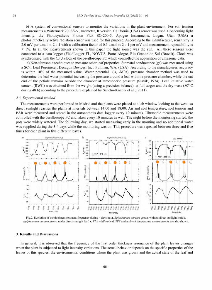
94 M.D. Fariñas et al. / Physics Procedia 63 ( 2015 ) 91 – 96

b) A system of conventional sensors to monitor the variations in the plant environment: For soil tensionmeasurements a Watermark 200SS-V, Irrometer, Riverside, California (USA) sensor was used. Concerning light intensity, the Photosynthetic Photon Flux SQ-200-5, Apogee Instruments, Logan, Utah (USA) a photosinthetically active radiation sensor was used for this purpose. According to the manufacturer, sensitivity is 2.0 mV per μmol m-2 s-1 with a calibration factor of 0.5 μmol m-2 s-1 per mV and measurement repeatability is < 1%. In all the measurements shown in this paper the light source was the sun. All these sensors were connected to a data logger (FieldLogger FL, NOVUS, Porto Alegre, Rio Grande do Sul (Brazil)). Clock was synchronized with the CPU clock of the oscilloscope PC which controlled the acquisition of ultrasonic data.

c) Non-ultrasonic techniques to measure other leaf properties: Stomatal conductance (gs) was measured usinga SC-1 Leaf Porometer, Decagon Devices, Inc., Pullman, WA, (USA). According to the manufacturer, accuracy is within 10% of the measured value. Water potential (ψ, -MPa), pressure chamber method was used to determine the leaf water potential increasing the pressure around a leaf within a pressure chamber, while the cut end of the petiole remains outside the chamber at atmospheric pressure (Slavik, 1974). Leaf Relative water content (RWC) was obtained from the weight (using a precision balance), at full turgor and the dry mass (80º C during 48 h) according to the procedure explained by Sancho-Knapik et al., (2011).

2.3. Experimental method The measurements were performed in Madrid and the plants were placed at a lab window looking to the west, so

direct sunlight reaches the plants at intervals between 14:00 and 18:00. Air and soil temperature, soil tension and PAR were measured and stored in the autonomous data logger every 10 minutes. Ultrasonic measurements were controlled with the oscilloscope PC and taken every 10 minutes as well. The night before the monitoring started, the pots were widely watered. The following day, we started measuring early in the morning and no additional water was supplied during the 3-4 days while the monitoring was on. This procedure was repeated between three and five times for each plant in five different leaves.

3. Results and Discussions

In general, it is observed that the frequency of the first order thickness resonance of the plant leaves changeswhen the plant is subjected to light intensity variations. The actual behavior depends on the specific properties of the leaves of this species, the environmental conditions where the plant was grown and the actual state of the leaf and

Fig.2. Evolution of the thickness resonant frequency during 4 days in: a, Epipremnum aureum grown without direct sunlight leaf; b, Epipremnum aureum grown under direct sunlight leaf; c, Vitis vinifera leaf. PPF and ambient temperature measurements are also shown.

- 66 -

M.D. Fariñas et al. / Physics Procedia 63 ( 2015 ) 91 – 96 95

the plant itself. It is expected that the technique can be equally applied to any other species, whenever thickness resonances of the leaves can be measured, though the actual behavior will depend on the specific features of the species and the plant under study.

Measured variation in the leaf properties due to the variations in the plant activity along the diurnal cycle are shown in Figures 2 a-c. They show the variation in the resonant frequency, the ambient temperature and the light intensity with the time of day. In addition, the expected value of fres at the turgor loss point (TLP) is also shown. In general, the variation in the thickness resonant frequency of the leaves with the time of day follows the variations in the light intensity (PPF). The sensitivity of fres to PPF varies between different species, but in all cases it has been observed that the minimum value of fres is obtained at the maximum value of PPF that, in our experimental set-up, was achieved between 1:00PM and 6:00PM.

The maximum relative variation of the thickness resonance is as follows: Epipremnum aureum (I): 5 ≥ 1 %; Epipremnum aureum (II): 7.5 ≥ 1 %; and Vitis vinifera: 12.5 ≥ 1 %. If we compare with

we observe two different types of behavior. For Epipremnum aureum the former is considerably smaller; while for Vitis vinifera both magnitudes are similar. In addition, in Epipremnum aureum (I) and Vitis vinifera, it is possible to observe a slight reduction of the maximum value of the resonant frequency reached during the night as the number of days of monitoring increases. This can be attributed to the progressive decay of the soil water content.

Table 2. RWC, water potential and maximum resonance frequency relative variation values at Turgor loss point (TLP).

Species

Turgor loss point (TLP).

RWC Water

potential (-MPa)

(%)

Epipremnum aureum 0.96 0.52 10 Vitis vinifera 0.9 1.99 13

4. Summary and Conclusions

This work shows that the presented air-coupled and wide band ultrasonic technique is able to detect, in a non-destructive, non-invasive, non-contact and fast way, variations in the leaves thickness resonances due to the response of the plant to variations in the light intensity. Decrease in light intensity (from 2000 to 150 μmol m-2 s-1) produces an increase in the leaf thickness resonant frequency (between 8% and 12%, depending on the species). This is explained by the reduction of plant transpiration, the closure of stomata and the concomitant shift of the water equilibrium in the leaves. Observed variations in the resonant frequency along the diurnal cycle (4%-10%) largely reflect the variations in light intensity. In addition, the kinetic of this response and the presence of saturation levels seems to depend on the adaptive mechanisms of the plants to the available degree of sunlight intensity.

Acknowledgements

Authors acknowledge funding by the Spanish Ministry for Economy and Competitivity, project DPI2011-22438 and Botín Foundation grant given to M.D. Fariñas in La Residencia de Estudiantes.

References

Álvarez-Arenas TEG, 2010. Simultaneous determination of the ultrasound velocity and the thickness of solid plates from the analysis of thickness resonances using air-coupled ultrasound. Ultrasonics, 50(2):104-109.

Álvarez-Arenas TEG, 2013. Air-coupled piezoelectric transducers with active polypropylene foam matching layers. Sensors, 13(5): 5996–6013. Álvarez-Arenas TEG, Calás H, Cuello JE, Fernández AR, Muñoz M., 2010. Noncontact ultrasonic spectroscopy applied to the study of

polypropylene ferroelectrets. J Appl Phys, 108(7):074110, 1-9. Álvarez-Arenas TEG, Sancho-Knapik D, Peguero-Pina JJ, Gil-Pelegrín E., 2009a. Noncontact and noninvasive study of plant leaves using air-

coupled ultrasounds. Appl Phys Lett. 95(19): 193702,1-3.

- 67 -

96 M.D. Fariñas et al. / Physics Procedia 63 ( 2015 ) 91 – 96

Álvarez-Arenas TEG, Sancho-Knapik D, Peguero-Pina JJ, Gil-Pelegrín E., 2009b. Determination of Plant Leaves Water Status using Air-Coupled Ultrasounds. IEEE International Ultrasonics Symposium. pp: 771–774.

Álvarez-Arenas TEG, Shrout TR, Zhang SJ, Lee HJ., 2013a. Air-Coupled Transducers Based on 1-3 Connectivity Single Crystal Transducers. IEEE International Ultrasonics Symposium 2010, 2230–2233.

Álvarez-Arenas TEG, Díez L, 2013b. Novel Impedance Matching Materials and Strategies for Air-Coupled Piezoelectric Transducers. IEEE Sensors. (in press).

Álvarez-Arenas, T.E.G., 2004. Acoustic impedance matching of piezoelectric transducers to the air. IEEE Trans Ultrason Ferroelec Freq Contr. 2004;51(5):624-633.

Álvarez-Arenas, T.E.G., Montero De Espinosa, F.R., Moner-Girona, M, Rodrıguez, E, Roig, A, Molins, E, 2002. Viscoelasticity of silica aerogels at ultrasonic frequencies. Applied Physics Letters, 81(7), p.1198.

Fariñas MD, Sancho-Knapik D, Peguero-Pina JJ, Gil-Pelegrín E, Álvarez-Arenas TEG., 2013. Shear waves in vegetal tissues at ultrasonic frequencies. App Phys Lett;102(10): 103702-103705.

Fukuhara M., 2002. Acoustic characteristics of botanical leaves using ultrasonic transmission waves. Plant Sci.;162(4):521-528. Givnish TJ., 1988. Adaptation to sun and shade: a whole-plant perspective. Functional Plant Biol.;15(2):63-92. Haller MI, Edward L, Khuri-Yakub BT., 1992. 1-3 Composites for Ultrasonic Air Transducers. IEEE Ultrasonics Symposium. 1992;2:937-939. Onoda Y, Schievig F, Anten NPR., 2008. Effects of Light and Nutrient Availability on Leaf Mechanical Properties of Plantago major: A

Conceptual Approach. Annals of Botany.;101:727-36. Sancho-Knapik D, Álvarez-Arenas TEG, Peguero-Pina JJ, Fernández V, Gil-Pelegrín E., 2011. Relationship between ultrasonic properties and

structural changes in the mesophyll during leaf dehydration. J Exp Bot.;62(10):3637–3645. Sancho-Knapik D, Álvarez-Arenas TEG, Peguero-Pina JJ, Gil-Pelegrín E., 2010. Air-coupled broadband ultrasonic spectroscopy as a new non-

invasive and non-contact method for the determination of leaf water status. J Exp Bot.;61(5): 1385–1391. Sancho-Knapik D, Calás H, Peguero-Pina JJ, Ramos Fernández A, Gil-Pelegrín E, Álvarez-Arenas TEG., 2012. Air-Coupled Ultrasonic

Resonant Spectroscopy for the Study of the Relationship Between Plant Leaves’ Elasticity and Their Water Content. IEEE Trans Ultrason Ferroelec Freq Contr. 2012;59(2):319–325.

Sancho-Knapik D, Peguero-Pina JJ, Fariñas MD, Álvarez-Arenas TEG, Gil-Pelegrín E., 2013. Ultrasonic spectroscopy allows a rapid determination of the relative water content at the turgor loss point: a comparison with pressure-volume curves in 13 woody species. Tree Physiol.;33(7):695–700.

Schindel DW, Hutchins DA., 1995. Through-thickness characterization of solids by wideband air-coupled ultrasound. Ultrasonics.:33(1);11-17. Scholander PF, Bradstreet ED, Hemmingsen EA, Hammel HT., 1965. Sap pressure in vascular plants negative hydrostatic pressure can be

measured in plants. Science.;148(3668):339-346. Slavík B., 1974. Methods of studying plant water relations. Berlin: Springer. Yano T, Tone M, Fukumoto A., 1987. Range finding and surface characterization using high-frequency air transducers. IEEE Trans Ultrason

Ferroelec Freq Contr.1987;34(2):232–236.

- 68 -

CAPÍTULO 5

CAPÍTULO 5.Caracterización de los Diferentes Tejidos que

Constituyen las Hojas de Phormium tenax

- 69 -

M.D. FARIÑAS, 2016

- 70 -

"Quegli che pigliavano per altore altro che la natura, maestra de’ maestri, s’affaticavano invano."

Leonardo da Vinci

CAPÍTULO 5

En este capítulo, se estudian las hojas en una especie muy particular: el Phormium tenax. La diversidad en los tejidos que componen su hoja, permitía aplicar diversas técnicas y configuraciones ultrasónicas a nuestro alcance para su completa caracterización. Además, dado el tradicional interés sobre sus fibras, pudimos contrastar medidas mecánicas con algunas recogidas en la bibliografía previa. La heterogeneidad mecánica existente entre los diferentes tipos de células del Phormium tenax, nos permitió ahondar en la dualidad forma-función y en el concepto de diseño multifuncional de los tejidos biológicos.

Los resultados preliminares sobre este estudio fueron presentados oralmente en el congreso internacional cuya referencia es:

FARIÑAS, M.D. y ÁLVAREZ-ARENAS, T.E.G., 2013. Non-invasive ultrasonic techniques to determine the elastic constants of layered vegetal parenchyma tissues and structural fibres: relationship with cellular microscopic features. 5th International Conference on Mechanics of Biomaterials and Tissues 2013. Sitges (España). Este trabajo puede consultarse en el siguiente enlace: https://us-biomat.com/events-media/congresses/icmobt-2013/

En esta comunicación oral, se presentaron las diferentes técnicas ultrasónicas empleadas para la caracterización de diferentes tejidos vegetales que podemos encontrar en las hojas de plantas así como la relación de los parámetros obtenidos con la microestructura.

Posteriormente, se publicaron los resultados completos en una revista científica indexada, que a continuación se incluye, y cuya referencia es:

FARIÑAS, M.D. y ÁLVAREZ-ARENAS, T.E.G., 2014. Ultrasonic assessment of the elastic functional design of component tissues of Phormium tenax leaves. Journal of the mechanical behavior of biomedical materials [en línea], vol. 39, pp. 304-15. [Consulta: 22 octubre 2014]. ISSN 1878-0180. DOI 10.1016/j.jmbbm.2014.07.018. Disponible en: http://www.ncbi.nlm.nih.gov/pubmed/25171747.

- 71 -

M.D. FARIÑAS, 2016

- 72 -

Available online at www.sciencedirect.com

www.elsevier.com/locate/jmbbm

j o u r n a l o f t h e m e c h a n i c a l b e h a v i o r o f b i o m e d i c a l m a t e r i a l s 3 9 ( 2 0 1 4 ) 3 0 4 – 3 1 5

http://dx.doi.org/10.1751-6161/& 2014 El

nCorresponding aE-mail addresses:

Research Paper

Ultrasonic assessment of the elastic functional designof component tissues of Phormium tenax leaves

M.D. Farinas, T.E.G. Alvarez-Arenasn

Sensors and Ultrasonic Technologies Department, Information and Physics Technologies Institute (ITEFI),Spanish National Research Council (CSIC), Serrano 144, 28006 Madrid, Spain

a r t i c l e i n f o

Article history:

Received 15 April 2014

Received in revised form

6 July 2014

Accepted 17 July 2014

Available online 14 August 2014

Keywords:

Phormium tenax leaf

Functional design

Ultrasound, Vegetal tissues

Tissue mechanical properties

Form and function

Fiber reinforced composites

1016/j.jmbbm.2014.07.018sevier Ltd. All rights rese

uthor.md.farinas@csic.es (M.D

a b s t r a c t

Different tissues in Phormium tenax leaves present different morphologies and mechanical

properties according to the different roles or functions that they play during the plant life.

This is an example of what is known as functional design, a concept which is used in

different scientific fields. Four different ultrasonic techniques comprising air-coupling and

gel coupling, longitudinal and shear waves, normal and oblique incidence and low

(0.2 MHz) and high frequencies (2.25 MHz) have been employed to study these leaves. By

changing these experimental conditions it is possible to propagate longitudinal and shear

waves in the different tissues present in these leaves (spongy mesophyll, chlorenchyma

and sclerenchyma fibres) and in different directions so it is possible to determine their

ultrasonic properties (velocity and attenuation) and hence their main elastic mudulii.

Additional analysis of microscopic images of the tissues permit to study the correlation

between this elastic and ultrasonic tissues properties and main microscopic features like

cell size and cell wall thickness, which are determined by the different function of these

tissues.

& 2014 Elsevier Ltd. All rights reserved.

rved.

. Fariñas), t.gomez@csic.es (T.E.G. Álvarez-Arenas).

- 73 -

1. Introduction

Functional Design is a concept used in engineering andsoftware and refers to a simplified design approach forcomplex systems. It is based on the assumptions that thesystem can be divided into several parts, that each of theseparts has only one function and that performs it with theminimum side effects on other parts. It is also used in biologywhere form and function are inseparable and is applied to thedifferent levels of biological organization (e.g. the morphologyof cells, the organization of tissues and the protein design), inthe sense that we can often guess how a biological entity

works by looking at its structure (Lodish et al., 2000). Inaddition, functional design space concept is also used in thefield of plant evolution (Niklas, 1997).

Phormium tenax, also known as New Zealand Flax is a

monocotyledonous plant belonging to the family Agavaceae;its leaves can be up to 3 m long, and contain very long and

strong fibers which account for 12–47% of the total cross-

sectional area of the leaf, depending on the variety (King andVincent, 1996). The research and use of these fibers as

reinforcement for eco-friendly natural fiber composites is atpresent going on (e.g. Duchemin et al., 2003; Harris et al.,

2005; Cruthers et al., 2006; Le Guen and Newman, 2007;

j o u r n a l o f t h e m e c h a n i c a l b e h a v i o r o f b i o m e d i c a l m a t e r i a l s 3 9 ( 2 0 1 4 ) 3 0 4 – 3 1 5 305

Newman et al., 2007; Wehi and Clarkson, 2014; Duchemin and

Staiger, 2009). Different techniques have been used to study

the mechanical properties of these fibers, comprising con-

ventional unidirectional stretching tests (De Rosa et al., 2010)

and propagation of shock waves (King and Vincent, 1996).

Different researches have reported fiber tensile strength in

the range 150 to 770 MPa (Jayaraman and Halliwell, 2009;

Santulli et al., 2009) and Young’s modulus from 10.4 up to

31.4 GPa.However, not only the fibers but also the whole leaves

have been the object of different studies. The presence ofthese strong fibers provides P. tenax leaves the character of aunidirectional fiber reinforced composite, which can belinked to the mechanical functional design of these leavesas it has been done before for grass leaves (Vincent, 1982).Mechanical measurements in different directions in thewhole leaf by King and Vincent (1996) have shown a long-itudinal and transverse stiffness of 3.9870.99 GPa and0.02270.002 GPa, respectively. Functional design of the cellwall has been studied by a Raman imaging approach byRichter et al. (2011).

Different sonic and ultrasonic techniques has also beenemployed to the study of plant leaves (Miller,1979; Zebrowski,1992; King and Vincent, 1996; Fukuhara, 2002; Wilson andDunton, 2009), though air-coupled ultrasonic techniques in athrough transmission configuration has only been recentlyapplied to excite and sense thickness resonances in plantleaves (Álvarez-Arenas et al., 2009a and Farinas et al., 2013a,2013b). From the analysis of the magnitude and phase spectraof the first order resonance it is possible to extract theeffective mechanical properties of the whole leaf in thedirection normal to the leaf plane. Moreover, if a widerfrequency spectrum is analyzed and several orders of thethickness resonances are observed, then it is possible toextract mechanical properties of the different layers oftissues that build up the leaf (mainly palisade parenchymaand spongy mesophyll) (Álvarez-Arenas et al., 2009b andFarinas et al., 2013a, 2013b).

The objective of this paper is to combine different ultra-sonic techniques to propagate different types of ultrasonicwaves (longitudinal and shear waves with different polariza-tion directions, at different frequencies) and along differentdirections. Depending on the technique used, the propaga-tion takes place along different paths within the leaf corre-sponding to different tissues so that it is possible to measurethe ultrasound propagation velocities in each of them andhence to work out their mechanical properties. Thesemechanical properties can be related with other tissuesfeatures, obtained from microscopic images, like cell shape,size, cell wall thickness and cell wall volume fraction, whichare determined by the function of each of these tissues and

Table 1 – Air-coupled transducers properties.

Centre frequency (MHz) Peak Sensitivity (dB) F

0.25 �25 00.65 �30 01.00 �32 0

- 74

cells, e.g. either mechanical support (strong unidirectionalfibers), or water transport/storage (parenchyma tissue andsheath cells), or gas interchange (soft spongy mesophyll),.

2. Materials and methods

2.1. Materials

2.1.1. Plant material and preparationSeveral P. tenax leaves of an unknown cultivar with lengthsbetween 1.2 and 1.8 m were harvested early in the morning.Leaves were then carried to the lab, and all measurementswere performed before noon. The basal section of theseleaves is folded along the midrib with the upper leaf surfaceon the inner fold, whereas the distal part is unfolded. Theupper leaf surface of the folded part formed an antrum fromthe basis on, but grew together before the leaf unfolded.Between 5 and 9 points were selected in each leaf along theleaf length in the unfolded leaf portion and all measurements(except those that involve wave propagation along the leaflength) were performed at these points. Once these measure-ments were finished, circles were excised using a punchholder to measure thickness and density. In addition sampleswere cut for observation with an optical microscope (seeSection 2.2.4). Measurements were repeated several timesalong the year, in June and September (2013) and January andMarch (2014).

2.1.2. Ultrasonic equipmentThree pairs of wide band and high sensitivity air-coupledultrasonic piezoelectric transducers designed and built atCSIC were used. Transducers properties are listed in Table 1.

In addition, for through transmission and direct contact(gel coupling) measurements of longitudinal waves weemployed a pair of 1.00 MHz Panametrics transducers(V314), and for ultrasonic propagation along the leaf lengthwe used 0.25 MHz Panametrics transducers (V1012). As cou-pling medium between transducers and leaves we used theOlympus ultrasonic couplant gel. Commercial Panametrics2.25 MHz shear wave transducers (V154) were used for shearwave measurements. As coupling medium we used thePanametrics ultrasonic shear couplant gel (SWC).

A Panametrics 5077 pulser/receiver was used for all theultrasonic measurements. The pulser provides a semicycle ofa square voltage signal to drive the transmitter transducer;amplitude of the excitation signal was set to 200 V for air-coupled measurements and to 100 V for the rest of themeasurements; pulser frequency was tuned to the transducercentre frequency. Low Pass filter was set off and High Passfilter was set to 10 MHz. The pulser also provides a

requency band (MHz) Radiating surface diameter (mm)

.1–0.35 20

.35–0.95 15

.50–1.30 10

-

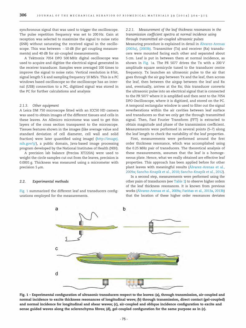
j o u r n a l o f t h e m e c h a n i c a l b e h a v i o r o f b i o m e d i c a l m a t e r i a l s 3 9 ( 2 0 1 4 ) 3 0 4 – 3 1 5306

synchronous signal that was used to trigger the oscilloscope.The pulse repetition frequency was set to 200 Hz. Gain atreception was selected to maximize the signal to noise ratio(SNR) without saturating the received signal in the oscillo-scope. This was between �10 dB (for gel coupling measure-ments) and 40 dB for air-coupled measurements.

A Tektronix 7054 DPO 500 MHz digital oscilloscope wasused to acquire and digitize the electrical signal generated inthe receiver transducer. Samples were averaged 100 times toimprove the signal to noise ratio. Vertical resolution is 8 bit,signal length 5 k and sampling frequency 10 MS/s. This is a PCwindows based oscilloscope so the oscilloscope has an inter-nal (USB) connection to a PC, digitized signal was stored inthe PC for further calculations and analysis

2.1.3. Other equipmentA Leica DM 750 microscope fitted with an ICC50 HD camerawas used to obtain images of the different tissues and cells inthese leaves. An Allmicro microtome was used to get thinlayers of the cross section transparent to the microscope.Tissues features shown in the images (like average value andstandard deviation of cell diameter, cell wall and solidfraction) were later quantified using imageJ (http://imagej.nih.gov/ij/), a public domain, Java-based image processingprogram developed by the National Institutes of Health (NIH).

A precision lab balance (Precisa XT220A) were used toweight the circle samples cut out from the leaves, precision is0.0001 g. Thickness was measured using a micrometer withprecision 5 μm.

2.2. Experimental methods

Fig. 1 summarized the different leaf and transducers config-urations employed for the measurements.

Fig. 1 – Experimental configuration of ultrasonic transducers resnormal incidence to excite thickness resonances of longitudinaland normal incidence for longitudinal and shear waves; (c), air-sense guided waves along the sclerenchyma fibres; (d), gel-coup

- 75

2.2.1. Measurement of the leaf thickness resonances in thetransmission coefficient spectra at normal incidence usingthrough transmitted air-coupled ultrasonic pulsesMeasuring procedure is explained in detail in Álvarez-Arenas(2003a), (2003b). Transmitter (Tx) and receiver (Rx) transdu-cers were mounted facing each other and separated about5 cm. Leaf is put in between them at normal incidence, asshown in Fig. 1a. The PR 5077 drives the Tx with a 200 Vamplitude square semicycle tuned to the transducer centrefrequency. Tx launches an ultrasonic pulse to the air thatgoes through the air gap between Tx and the leaf, then acrossthe leaf, then between the airgap between the leaf and Rxand, eventually, arrives at the Rx; this transducer convertsthe ultrasonic pulse into an electrical signal that is connectedto the PR 5077 where it is amplified and then sent to the 7054DPO Oscilloscope, where it is digitized, and stored on the PC.A temporal rectangular window is used to filter out the signalreverberations within the air cavities between leaf surfaceand transducers so that we only get the through transmittedsignal. Then, Fast Fourier Transform (FFT) is extracted toobtain magnitude and phase of the transmission coefficient.Measurements were performed in several points (5–7) alongthe leaf length to check the variability of the leaf properties.

First, measurements were performed around the firstorder thickness resonance, which was accomplished usingthe 0.25 MHz pair of transducers. The theoretical analysis ofthese measurements, assumes that the leaf is a homoge-neous plate. Hence, what we really obtained are effective leafproperties. This approach has been applied before for otherplant leaves with meaningful results (Álvarez-Arenas et al.,2009a; Sancho-Knapik et al., 2010; Sancho-Knapik et al., 2012).

In a second step, measurements were performed using theother pairs of transducers (see Table 1) to observe higher ordersof the leaf thickness resonances. It is known from previousworks (Álvarez-Arenas et al., 2009a; Farinas et al., 2013a, 2013b)that the location of these higher order resonances deviates

pect to the leaves: (a), through transmission, air-coupled andwave; (b) through transmission, direct contact (gel-coupled)coupled and oblique incidence configuration to excite andled configuration for the same purpose as in (c).

-

j o u r n a l o f t h e m e c h a n i c a l b e h a v i o r o f b i o m e d i c a l m a t e r i a l s 3 9 ( 2 0 1 4 ) 3 0 4 – 3 1 5 307

from the predictions of the one layer model, and that this is dueto layered structure of the leaf in the thickness direction.Therefore using a layered model permit us to get a better fittingof the theoretical calculations into the experimental data, andmakes it possible to extract material properties of the differentlayers of tissue that made up the leaves (Farinas et al., 2013a,2013b). Further details of both procedures are given in Section2.3.

2.2.2. Measurement of the velocity of longitudinal and shearultrasonic waves in the leaf thickness direction using gelcoupling in through transmission configurationExperimental set-up is schematically shown in Fig. 1b. Thetwo V314 Panametrics 1.00 MHz transducers were firstattached one directly to the other using gel coupling. Txwas then driven by the PR 5077 and the received signal wasstored in the DPO 5074 Oscilloscope. Then, we put the leaf inbetween the transducers and measure the time delaybetween this signal and the signal received when bothtransducers were in direct contact. From this time delayand the leaf thickness measured at the same point using amicrometer, we worked out the ultrasound velocity.

The procedure for the shear wave measurements usingthe 2.25 MHz shear wave transducers (V154) is similar as theone explained before and Fig. 1b also corresponds to thisconfiguration. In this case, there are two significant differ-ences though. First the gel couplant used in this case is a veryviscous one, able to transmit shear waves. The second onerefers to the nature of the wave; in this case the transducersgenerate linearly polarized shear waves, the propagationdirection is normal to the leaf plane, and the shear displace-ment takes place in the leaf plane. As the leaf can beconsidered as a unidirectional fiber reinforced composite,then there are two different main velocities and we measuredboth of them; they correspond to the shear waves with thedirection of polarization along and normal to the fibres,respectively.

2.2.3. Measurement of the velocity of ultrasonic waves in theleaf plane along the sclerenchyma fibers directionTwo different techniques were used for this purpose.

1. Air-coupled 0.25 MHz centre frequency transducers andoblique incidence to generate guided lateral longitudinalwaves that propagates along the fibres. Employed techniqueis the same as used to excite plate waves using the Kremer’srule also called coincidence principle (Cremer., 1947;Brekhovskikh, 1960). Experimental set-up is schematicallyshown in Fig. 1c. This technique has been widely used inthe past to excite Lamb waves in plates and in fiber reinforcedpolymer plates. The incidence angle of the ultrasonic radia-tion in the leaf is set so that the projection of the wave lengthof the incident field coincides with the wave length of thelongitudinal waves guided in the fibres, so that a resonantcondition is achieved and this mode is generated. The wavepropagates along the leaf length and a second transducerfacing the leaf at the same angle (but opposite direction)receives the leakage of the wave to the air. This secondtransducer is displaced along the leaf length in steps of1.6 mm over a total distance of 100 mm. At each step thereceived signal is recorded. As the distance between

- 76

transducers is increased the time delay in the received signalis increased. Time delay is plotted against the distance and itprovides a straight line, from the slope of this line we obtainthe ultrasound velocity for the propagation in the plane ofthe leaf.

2. The two gel coupled 0.25 MHz transducers wereattached using the coupling gel to the same side of the leafbut separated by a few centimeters. Experimental set-up isschematically shown in Fig. 1d. The Tx is driven as inprevious cases and the received signal in Rx is stored. The,Rx transducer is moved away 1 cm, and the process isrepeated. The time delay is recorded for each distance andfrom the graph distance versus time delay we obtain theultrasound velocity in the leaf plane along the leaf fibersdirection. This procedure has also been used in the past todetermine velocity of Lamb waves (Szewieczek et al., 2012).

2.2.4. Other non ultrasonic methodsOnce the ultrasonic measurements were finished, circleswere excised from the leaves at the marked points using apunch holder (10 mm diam.). Disk thickness was measuredwith a micrometer, weighed using the precision balance, and,finally, density was worked out. Then, the excised leaf circleswere put in an oven at 80 C for 48 h to remove the water;finally, they were removed from the oven and weighed againto get the dry matter content.

Tissue structure was investigated and photographed forlater quantification with a light microscope (Leica DM 750)equipped with a digital camera (ICC50 HD). Two maindifferent kind of observation were performed: (i) cross-section of the leaves at different points along the leaf length(ii) surface of the leaves after removal of the epidermis. Maintissues features like cell diameter, cell wall and/or solidfraction were later quantified using imageJ, a public domain,Java-based image processing program developed by theNational Institutes of Health (NIH).

2.3. Theoretical methods

2.3.1. Analysis of the first thickness resonance measured byusing air-coupled ultrasound and a through transmissionconfiguration: Effective medium approachThe measured spectra of the transmission coefficient ofdifferent plant leaves in the frequency range limited aroundthe first order thickness resonance can be reproduced by atheoretical model that assumes the leaf as a homogeneousand flat plate and considers normal incidence (Álvarez-Arenas et al., 2009b). In this case a simple analytical expres-sion can be derived for the transmission coefficient (γ), see Eq.(1), that depends on the acoustic impedance of the leaf andthe surrounding medium (air in this case): z1 and z2, respec-tively, the thickness of the leaf (t), the ultrasound velocity (c)and the attenuation (α) in the leaf and the ultrasoundfrequency (f).

γ ¼ �2Z1Z2

2Z1Z2 cos ðktÞ þ iðZ21 þ Z2

2Þ sin ðktÞ ð1Þ

where ω¼2πf, and k¼ω/c.

-

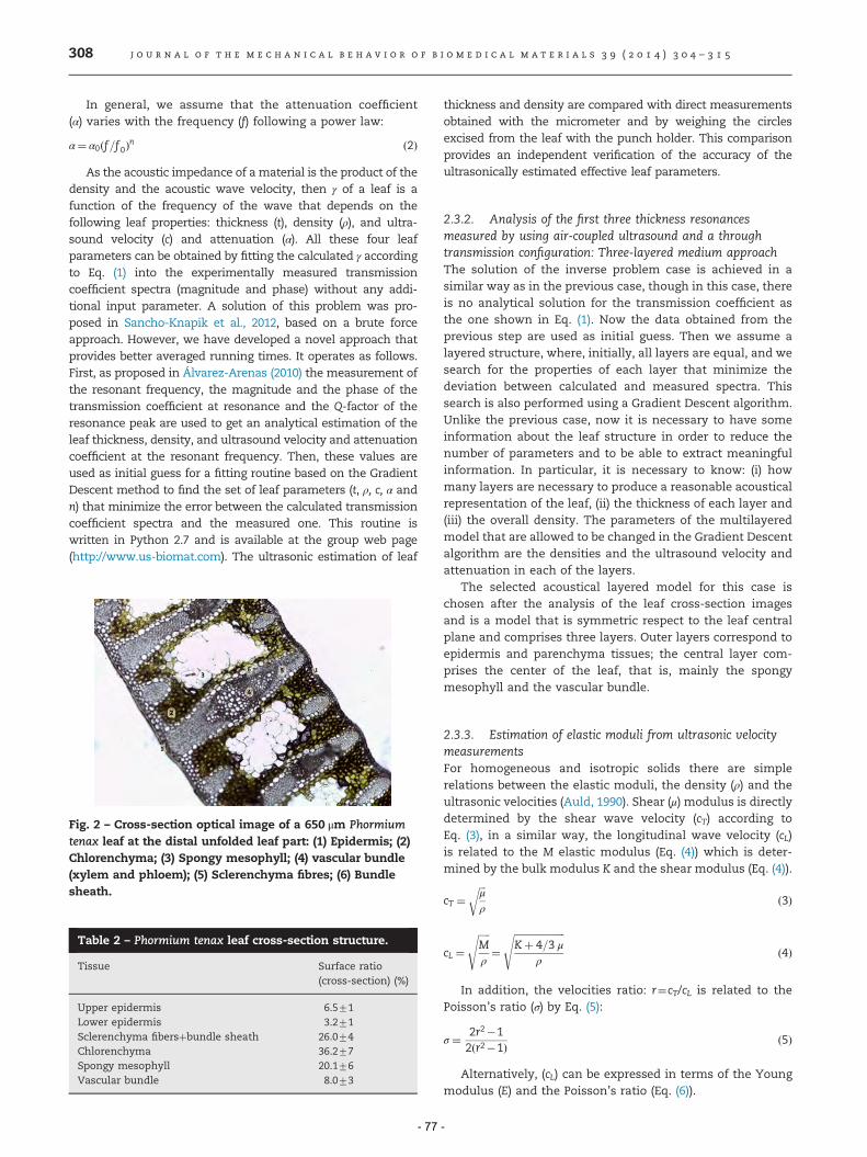
j o u r n a l o f t h e m e c h a n i c a l b e h a v i o r o f b i o m e d i c a l m a t e r i a l s 3 9 ( 2 0 1 4 ) 3 0 4 – 3 1 5308

In general, we assume that the attenuation coefficient(α) varies with the frequency (f) following a power law:

α¼ α0ðf=f 0Þn ð2Þ

As the acoustic impedance of a material is the product of thedensity and the acoustic wave velocity, then γ of a leaf is afunction of the frequency of the wave that depends on thefollowing leaf properties: thickness (t), density (ρ), and ultra-sound velocity (c) and attenuation (α). All these four leafparameters can be obtained by fitting the calculated γ accordingto Eq. (1) into the experimentally measured transmissioncoefficient spectra (magnitude and phase) without any addi-tional input parameter. A solution of this problem was pro-posed in Sancho-Knapik et al., 2012, based on a brute forceapproach. However, we have developed a novel approach thatprovides better averaged running times. It operates as follows.First, as proposed in Álvarez-Arenas (2010) the measurement ofthe resonant frequency, the magnitude and the phase of thetransmission coefficient at resonance and the Q-factor of theresonance peak are used to get an analytical estimation of theleaf thickness, density, and ultrasound velocity and attenuationcoefficient at the resonant frequency. Then, these values areused as initial guess for a fitting routine based on the GradientDescent method to find the set of leaf parameters (t, ρ, c, α andn) that minimize the error between the calculated transmissioncoefficient spectra and the measured one. This routine iswritten in Python 2.7 and is available at the group web page(http://www.us-biomat.com). The ultrasonic estimation of leaf

Fig. 2 – Cross-section optical image of a 650 μm Phormiumtenax leaf at the distal unfolded leaf part: (1) Epidermis; (2)Chlorenchyma; (3) Spongy mesophyll; (4) vascular bundle(xylem and phloem); (5) Sclerenchyma fibres; (6) Bundlesheath.

Table 2 – Phormium tenax leaf cross-section structure.

Tissue Surface ratio(cross-section) (%)

Upper epidermis 6.571Lower epidermis 3.271Sclerenchyma fibersþbundle sheath 26.074Chlorenchyma 36.277Spongy mesophyll 20.176Vascular bundle 8.073

- 77

thickness and density are compared with direct measurementsobtained with the micrometer and by weighing the circlesexcised from the leaf with the punch holder. This comparisonprovides an independent verification of the accuracy of theultrasonically estimated effective leaf parameters.

2.3.2. Analysis of the first three thickness resonancesmeasured by using air-coupled ultrasound and a throughtransmission configuration: Three-layered medium approachThe solution of the inverse problem case is achieved in asimilar way as in the previous case, though in this case, thereis no analytical solution for the transmission coefficient asthe one shown in Eq. (1). Now the data obtained from theprevious step are used as initial guess. Then we assume alayered structure, where, initially, all layers are equal, and wesearch for the properties of each layer that minimize thedeviation between calculated and measured spectra. Thissearch is also performed using a Gradient Descent algorithm.Unlike the previous case, now it is necessary to have someinformation about the leaf structure in order to reduce thenumber of parameters and to be able to extract meaningfulinformation. In particular, it is necessary to know: (i) howmany layers are necessary to produce a reasonable acousticalrepresentation of the leaf, (ii) the thickness of each layer and(iii) the overall density. The parameters of the multilayeredmodel that are allowed to be changed in the Gradient Descentalgorithm are the densities and the ultrasound velocity andattenuation in each of the layers.

The selected acoustical layered model for this case ischosen after the analysis of the leaf cross-section imagesand is a model that is symmetric respect to the leaf centralplane and comprises three layers. Outer layers correspond toepidermis and parenchyma tissues; the central layer com-prises the center of the leaf, that is, mainly the spongymesophyll and the vascular bundle.

2.3.3. Estimation of elastic moduli from ultrasonic velocitymeasurementsFor homogeneous and isotropic solids there are simplerelations between the elastic moduli, the density (ρ) and theultrasonic velocities (Auld, 1990). Shear (μ) modulus is directlydetermined by the shear wave velocity (cT) according toEq. (3), in a similar way, the longitudinal wave velocity (cL)is related to the M elastic modulus (Eq. (4)) which is deter-mined by the bulk modulus K and the shear modulus (Eq. (4)).

cT ¼ffiffiffiμ

ρ

rð3Þ

cL ¼ffiffiffiffiffiMρ

s

¼ffiffiffiffiffiffiffiffiffiffiffiffiffiffiffiffiffiffiffiffiffiKþ 4=3 μ

ρ

s

ð4Þ

In addition, the velocities ratio: r¼cT/cL is related to thePoisson’s ratio (σ) by Eq. (5):

σ ¼ 2r2�12ðr2�1Þ ð5Þ

Alternatively, (cL) can be expressed in terms of the Youngmodulus (E) and the Poisson’s ratio (Eq. (6)).

-

Fig. 3 – Details from P. tenax cross-section: (a) Chlorenchyma, chloroplasts are clearly seen (image horizontal width: 160 μm);(b) Sclerenchyma fibres (image horizontal width: 160 μm); (c) Spongy Mesophyll (image horizontal width: 220 μm); (d) Vascularbundle, sheath cells (larger cell without chloroplasts) can be seen surrounding the vascular bundle (image horizontal width:220 μm).

Table 3 – P. tenax cell and cell wall dimensions in the different leaf tissues.

Tissue Cell diameter (μm) Cell wall thickness (μm) Solid fraction ρn=ρS (%)

Eq. (9) Image Mean value

Chlorenchyma 26.475.6 0.7970.14 15 25 20Sclerenchyma 10.6772.3 3.7470.77 70 85 77.5Spongy mesophyll 44.6724.3 0.3570.07 5 10 7.5Bundle sheath 19.274.0 1.170.15 25 – 25

Fig. 4 – Leaf structure in the longitudinal plane below theepidermis: (1) Chlorenchyma tissue (green color is due to thechloroplasts); (2) Sclerenchyma fibres, individual cells(elongated and thick walled) can be seen. (For interpretation ofthe references to color in this figure legend, the reader isreferred to the web version of this article.)

j o u r n a l o f t h e m e c h a n i c a l b e h a v i o r o f b i o m e d i c a l m a t e r i a l s 3 9 ( 2 0 1 4 ) 3 0 4 – 3 1 5 309

- 78 -

cL ¼ffiffiffiffiffiffiffiffiffiffiffiffiffiffiffiffiffiffiffiffiffiffiffiffiffiffiffiffiffiffiffiffiffi

Eð1�σÞρð1þ σÞð1�2σÞ

s

ð6Þ

When material dimensions interfere with the ultrasonicpropagation, like in plates or rods, then different relationsexist between the elastic constants and the velocities. Forexample, in the case of plates, it is possible to excite a widecollection of guided waves called Lamb waves. In the parti-cular case of propagation in rods or bars where the wave-length is much larger than the rod diameter, the relationshipbetween the velocity and the Young’s modulus is given by:

cRod ¼ffiffiffiEρ

s

ð7Þ

For different leaves Poisson’s ratio values close to 0.33 hasbeen measured using ultrasonic means (Farinas et al., 2013a,2013b), and a value between 0.3 and 0.4 has been estimatedby King and Vincent, 1996 to calculate Young modulus valuesfrom longitudinal velocity measurements.

-60

-55

-50

-45

-40

-35

Mag

nitu

de (

dB) a

0.10 0.15 0.20 0.25 0.30 0.35 0.40-0.75

0.00

0.75

1.50

Pha

se (

rad)

Frequency (MHz)

Transmission Coefficient

b

Fig. 6 – Magnitude (a) and phase (b) spectra of transmissioncoefficient in 5 different points along the length of a P. tenaxleaf in the unfolded section (thickness: 0.97 mm, 0.85 mm,0.75 mm, 0.66 mm 0.52 mm); Circles: experimental data;Solid line: theoretically calculated values by the one-layer model.

600

700

800

900

1000

Den

sity

(kg

/m3 )

0.4 0.6 0.8 1.0 1.230

35

40

45

50

Dry

mat

ter

ratio

(%

)

Thickness (mm)

Fig. 5 – Density (a) and dry matter ratio (b) of P. tenax leavesin the unfolded leaf section vs. leaf thickness. Black circles:winter P. tenax leaves; blank circles: summer P. tenax leaves.

0.4 0.6 0.8 1.0 1.2

0.4

0.6

0.8

1.0

1.2

Thi

ckne

ss -

ultr

asou

nd-

(mm

)

Thickness -micrometer- (mm)

600 700 800 900 1000 1100 1200600

700

800

900

1000

1100

1200

Den

sity

-ul

tras

ound

- (k

g/m

3 )

Density -weight and size- (kg/m3)

Fig. 7 – (a) Thickness obtained by the ultrasonic techniquevs. thickness measured using a micrometer. (b) Densityobtained by the ultrasonic technique vs. density obtainedfrom the measured thickness and weight of the excisedcircles: black circles, values in winter P. tenax leaves; blankcircles, values in summer P. tenax leaves.

j o u r n a l o f t h e m e c h a n i c a l b e h a v i o r o f b i o m e d i c a l m a t e r i a l s 3 9 ( 2 0 1 4 ) 3 0 4 – 3 1 5310

Finally, assuming that the tissues are closed-cell cellularsolids (Gibson and Ashby, 1999), it is possible to estimate thecell wall Young modulus ðESÞ from the tissue Young modulusðEnÞ and the relative density ðρn=ρSÞ according to Eq. (7)

En

ES¼ ρn

ρS

� �2

¼ ð1�φÞ2 ð8Þ

where the superscript n denotes the cellular solid, and thesubscript S the solid in the cell wall; ð1�φÞ is the volumetricsolid fraction in the tissue. In addition, for closed-cell cellularsolids, it is also possible to establish an analytical relationshipbetween the ratio of cell wall length (l) to cell wall thickness (t)and the relative density ðρn=ρSÞ (Gibson and Ashby, 1999).

- 79 -

ρn=ρS ¼ Ct=l ð9Þ

where C depends on cell geometry. For some ideal cases, thevalue of C can be calculated, for example, it is 1.90 and 1.18 forrhombic dodecahedra and for tetrakaidecahedra cells,respectively.

3. Results

3.1. Optical microscopy images of the leaf tissues and thecellular structure

The structure of the P. tenax leaf has been the object ofprevious studies, further details can be seen in King andVincent, 1996; Richter et al., 2011; and Arévalo et al. (2013).Measurements were taken at the central part of the leaf(unfolded distal part) over a total distance of about 500 mm.Leaf thickness in this area varies typically from 500 μm up to1100 μm. Fig. 2 shows the typical structure of the studied P.tenax leaves. It comprises the adaxial and abaxial epidermis(1), the chlorenchyma (2), the spongy mesophyll (3), thevascular bundle (xylem and phloem) (4), the sclerenchymafibers (5) and the bundle sheath (6), that is the parenchyma-tous sheath that surrounds the vascular bundle. Chloroplastsare only present in the parenchyma tissue (2). Mean values

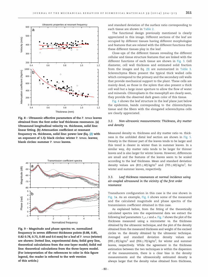
0.4 0.6 0.8 1.0 1.2200

300

400

500

600

Vel

ocity

(m

/s)

Ultrasonic properties at resonant frequency

0.4 0.6 0.8 1.0 1.20

200

400

600

800

1000

Atte

nuat

ion

coef

ficie

nt (

Np/

m)

Thickness (mm)

b

a

Fig. 8 – Ultrasonic effective parameters of the P. tenax leavesobtained from the first order leaf thickness resonance. (a)Ultrasound longitudinal velocity vs. thickness, solid line:linear fitting. (b) Attenuation coefficient at resonantfrequency vs. thickness, solid line: power law (Eq. (2) withan exponent of 1.5): black circles: winter P. tenax. leaves;blank circles: summer P. tenax leaves.

-80

-70

-60

-50

-40

Mag

nitu

de (

dB)

1 2 3 4 5-1

0

1

2

3

4

5

Pha

se (

rad)

Normalized frequency

Transmission coefficient spectra

Fig. 9 – Magnitude and phase spectra vs. normalizedfrequency in seven different thickness points (0.88, 0.85,0.82 0.78, 0.73, 0.68 and 0.6 mm) for a leaf of P. tenax (winter)are shown: Dotted line, experimental data; Solid grey line,theoretical calculations from the one-layer model; Solid redline: theoretical calculations from the three-layers model.(For interpretation of the references to color in this figurelegend, the reader is referred to the web versionof this article.)

j o u r n a l o f t h e m e c h a n i c a l b e h a v i o r o f b i o m e d i c a l m a t e r i a l s 3 9 ( 2 0 1 4 ) 3 0 4 – 3 1 5 311

- 80

and standard deviation of the surface ratio corresponding toeach tissue are shown in Table 2.

The functional design previously mentioned is clearlyappreciated in this image. Different sections of the leaf areoccupied by different tissues having different morphologiesand features that are related with the different functions thatthese different tissues play in the leaf.

Close-ups of the different tissues revealing the differentcellular and tissue structure features that are linked with thedifferent functions of each tissue are shown in Fig. 3. Celldiameter, cell wall thickness and estimated solid fractionfrom the images and Eq. (9) are summarized in Table 3.Sclerenchyma fibers present the typical thick walled cellswhich correspond to the primary and the secondary cell wallsthat provide mechanical support to the plant. These cells aremainly dead, as those in the xylem that also present a thickcell wall but a large inner aperture to allow the flow of waterand minerals. Chloroplasts in the mesophyll are clearly seen,they provide the observed dark green color of this tissue.

Fig. 4 shows the leaf structure in the leaf plane just belowthe epidermis, bands corresponding to the chlorenchymatissue and the fibers with the elongated sclerenchyma cellsare clearly appreciated.

3.2. Non-ultrasonic measurements: Thickness, dry matterand density

Measured density vs. thickness and dry matter ratio vs. thick-ness in the unfolded distal leaf section are shown in Fig. 5.Density in the thinner part of the leaves tends to be larger andthis trend is clearer in winter than in summer leaves. In asimilar way, dry matter ratio tends to be larger for thinnerleaves and is also larger for winter leaves. However, differencesare small and the features of the leaves seem to be scaledaccording to the leaf thickness. Mean and standard deviationdensity values are (815740) kg/m3 and (705760) kg/m3, forwinter and summer leaves, respectively.

3.3. Leaf thickness resonances at normal incidence usingair-coupled ultrasound in the vicinity of the first orderresonance

Transducers configuration in this case is the one shown inFig. 1a. As an example, Fig. 6 shows some of the measuredand the calculated magnitude and phase spectra of thetransmission coefficient obtained in this case.

As explained before, from the fitting of the theoreticallycalculated spectra into the experimental data we extract thefollowing leaf parameters: t, ρ, c and α. Fig. 7 shows the plot of thethickness measured using a micrometer vs. the thicknessobtained by the ultrasonic technique, and the plot of the densityobtained from themeasured thickness and weight of the excisedcircles vs. the density obtained by the ultrasonic technique.Averaged and standard deviation density values are(995785) kg/m3 and (956770) kg/m3, for winter and summerleaves, respectively. While the agreement in the thicknessestimation between the two techniques is within the dispersionof the measurements, there is a clear bias in the densitymeasurements and the ultrasonically estimated density isalways larger that the density value obtained from thickness,

-

Table 4 – Ultrasonic properties of different tissues of winter and summer P. tenax leaves.

Time ofyear

Tissue Density(kg/m3)

Ultrasound velocity(m/s)

Utrasound attenuation(Np/m)

M-elastic modulus(MPa)

Summer Spongy mesophyll 500715 450715 350710 (@ 250 kHz) 10077Epidermisþchlorenchyma 960720 560720 300720

Winter Spongy mesophyll 650715 420715 365710 (@ 250 kHz) 11577Epidermisþchlorenchyma 950720 500720 240720

0.4 0.6 0.8 1.0 1.2200

300

400

500

600

700

800

900

1000

1100

Ultr

asou

nd v

eloc

ity (

m/s

)

Thickness (mm)

Longitudinal

Shear II fibre

Shear fibre

Fig. 10 – Ultrasound velocity measurements for longitudinaland shear waves (both in fibres direction and perpendicularto them) vs. thickness in winter P. tenax. leaves: Dot,experimental data; Solid line, linear fitting.

j o u r n a l o f t h e m e c h a n i c a l b e h a v i o r o f b i o m e d i c a l m a t e r i a l s 3 9 ( 2 0 1 4 ) 3 0 4 – 3 1 5312

section and weight measurements. This can be explained by thelayered structure of the leaf and the relatively larger density ofthe tissues at the leaf surface (see Section 4).

Ultrasound velocity and attenuation coefficient (measuredat the resonant frequency) vs. thickness are shown in Fig. 8 Inthe case of the velocity results, the solid line represent a linearfitting, for attenuation data, the solid line is, following Eq. (2), apower law fitting (vs. thickness) with an exponent of 1.5.Measured velocities are comparable to the values measuredbefore for leaves of other species. Attenuation values are verylarge (200–800 Np/m, for frequencies between 200 and 300 kHz),and are also similar to other values found before. This largeattenuation coefficient is due to the complex and porousstructure of the leaf. Winter leaves present a slightly largevelocity values while velocity is rather independent of thethickness, and the attenuation coefficient increases as thethickness decreases. This is due to the fact that measurementsat thinner leaf sections are taken at a larger frequency (seeFig. 6), and attenuation increases with the frequency (Eq. (2)).

3.4. Leaf thickness resonances at normal incidence usingair-coupled ultrasound over a wider frequency range (severalorders of the thickness resonances)

The experimental set-up is the same as in the previous case, butnow, a larger frequency band is analyzed. As an example of theobtained results, measured and calculated spectra of the trans-mission coefficient for one leaf at seven different points havingdifferent thickness (0.88, 0.85, 0.82 0.78, 0.73, 0.68 and 0.6mm) areshown in Fig. 9. To get a clearer representation of all these data,magnitude and phase spectra are plotted against the normalizedfrequency where the frequency of the first order thicknessresonance is used to normalize the frequency axis. Gray solidline corresponds to the calculated spectra assuming the leaf as ahomogeneous layer and using the parameters obtained in theprevious section (Section 3.2). As it has previously been observedfor other species (Álvarez-Arenas et al., 2009a and Farinas et al.,2013a, 2013b), the one layer homogeneous model fails to predictthe leaf response outside this narrow frequency window. Redsolid line represents the calculated values obtained with thethree layers model as explained in Section 2.3. Obtained proper-ties of each of these layers from the fitting of the theoreticallycalculated transmission coefficient spectra into the experimentaldata are shown in Table 4.

As expected, spongy mesophyll presents a lower densityand a lower velocity. If a Poisson’s ratio value of 0.33 (Farinaset al., 2013a, 2013b) is assumed, then it is possible to obtainthe tissue’s Young’s modulus (Eq. (6)), and with the relativedensity values in Table 3 it is possible to calculate the cellwall Young’s modulus. These estimations appear in Table 5.

- 81

3.5. Through transmission ultrasonic longitudinal andshear wave measurements in the direction normal to the leafplane using gel coupling

Measurements were performed with the transducers and leafconfiguration shown in Fig. 1b using the 1.00 MHz longitudi-nal wave transducers and the 2.25 MHz shear wave transdu-cers. In all cases propagation took place in the directionnormal to the leaf plane. For the case of the shear wave,measurements for two different polarizations were per-formed: along the fiber direction and normal to the fiberdirection. Results are shown in Fig. 10 for winter leaves.Straight lines represent a linear fitting.

Mean values and standard variation are: (762798.6) m/s,for the longitudinal wave, and (268.9725.3) m/s and(572.8781.2) m/s for the shear waves with polarization inthe fiber direction and normal to it, respectively. In this case,longitudinal wave propagation takes place most likelythrough the fibers and the sheath cells (and this can be thereason for the differences with the longitudinal velocityvalues presented in previous sections, a further analysis isin Section 4). If we assume a density of 950 kg/m3, then theM-elastic modulus is 550 MPa, which is a much larger valuethan those obtained before for the chlorenchyma and thespongy mesophyll. A more detailed analysis of these resultsin terms of material elastic constants must take into accountthe composite and anisotropic nature of this tissue.

-

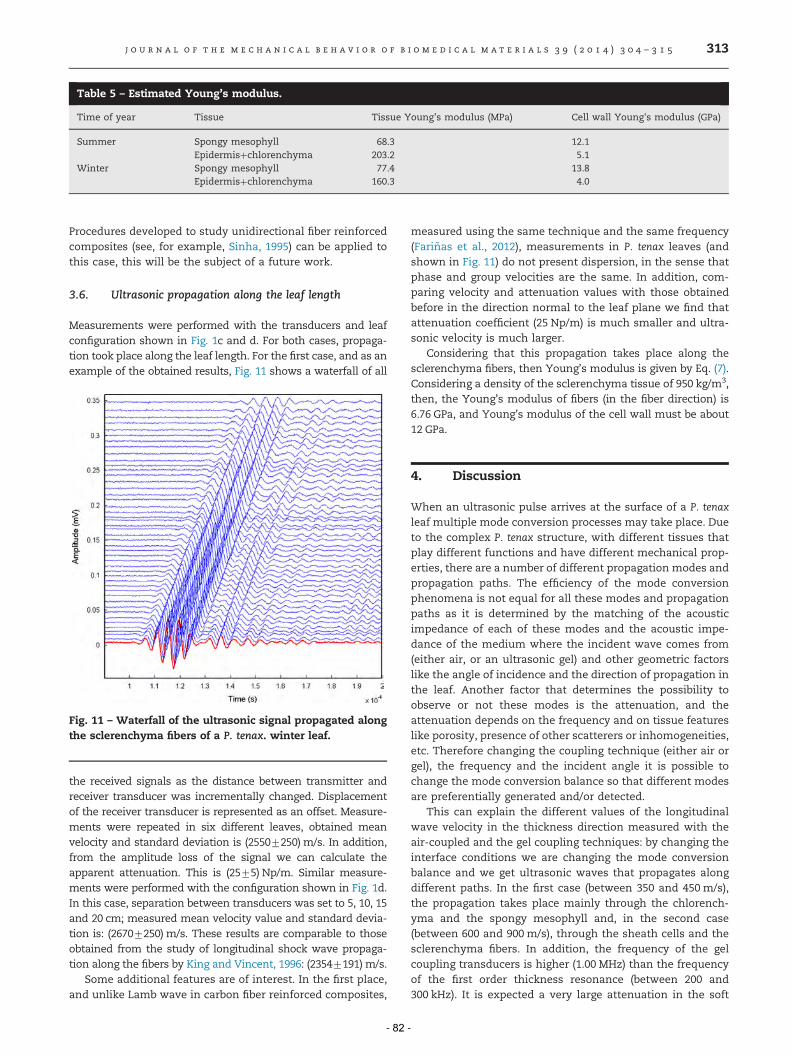
Table 5 – Estimated Young’s modulus.

Time of year Tissue Tissue Young’s modulus (MPa) Cell wall Young's modulus (GPa)

Summer Spongy mesophyll 68.3 12.1Epidermisþchlorenchyma 203.2 5.1

Winter Spongy mesophyll 77.4 13.8Epidermisþchlorenchyma 160.3 4.0

j o u r n a l o f t h e m e c h a n i c a l b e h a v i o r o f b i o m e d i c a l m a t e r i a l s 3 9 ( 2 0 1 4 ) 3 0 4 – 3 1 5 313

Procedures developed to study unidirectional fiber reinforcedcomposites (see, for example, Sinha, 1995) can be applied tothis case, this will be the subject of a future work.

3.6. Ultrasonic propagation along the leaf length

Measurements were performed with the transducers and leafconfiguration shown in Fig. 1c and d. For both cases, propaga-tion took place along the leaf length. For the first case, and as anexample of the obtained results, Fig. 11 shows a waterfall of all

Fig. 11 – Waterfall of the ultrasonic signal propagated alongthe sclerenchyma fibers of a P. tenax. winter leaf.

the received signals as the distance between transmitter andreceiver transducer was incrementally changed. Displacementof the receiver transducer is represented as an offset. Measure-ments were repeated in six different leaves, obtained meanvelocity and standard deviation is (25507250) m/s. In addition,from the amplitude loss of the signal we can calculate theapparent attenuation. This is (2575) Np/m. Similar measure-ments were performed with the configuration shown in Fig. 1d.In this case, separation between transducers was set to 5, 10, 15and 20 cm; measured mean velocity value and standard devia-tion is: (26707250) m/s. These results are comparable to thoseobtained from the study of longitudinal shock wave propaga-tion along the fibers by King and Vincent, 1996: (23547191) m/s.

Some additional features are of interest. In the first place,and unlike Lamb wave in carbon fiber reinforced composites,

- 82

measured using the same technique and the same frequency(Fariñas et al., 2012), measurements in P. tenax leaves (andshown in Fig. 11) do not present dispersion, in the sense thatphase and group velocities are the same. In addition, com-paring velocity and attenuation values with those obtainedbefore in the direction normal to the leaf plane we find thatattenuation coefficient (25 Np/m) is much smaller and ultra-sonic velocity is much larger.

Considering that this propagation takes place along thesclerenchyma fibers, then Young’s modulus is given by Eq. (7).Considering a density of the sclerenchyma tissue of 950 kg/m3,then, the Young’s modulus of fibers (in the fiber direction) is6.76 GPa, and Young’s modulus of the cell wall must be about12 GPa.

4. Discussion

When an ultrasonic pulse arrives at the surface of a P. tenaxleaf multiple mode conversion processes may take place. Dueto the complex P. tenax structure, with different tissues thatplay different functions and have different mechanical prop-erties, there are a number of different propagation modes andpropagation paths. The efficiency of the mode conversionphenomena is not equal for all these modes and propagationpaths as it is determined by the matching of the acousticimpedance of each of these modes and the acoustic impe-dance of the medium where the incident wave comes from(either air, or an ultrasonic gel) and other geometric factorslike the angle of incidence and the direction of propagation inthe leaf. Another factor that determines the possibility toobserve or not these modes is the attenuation, and theattenuation depends on the frequency and on tissue featureslike porosity, presence of other scatterers or inhomogeneities,etc. Therefore changing the coupling technique (either air orgel), the frequency and the incident angle it is possible tochange the mode conversion balance so that different modesare preferentially generated and/or detected.

This can explain the different values of the longitudinalwave velocity in the thickness direction measured with theair-coupled and the gel coupling techniques: by changing theinterface conditions we are changing the mode conversionbalance and we get ultrasonic waves that propagates alongdifferent paths. In the first case (between 350 and 450 m/s),the propagation takes place mainly through the chlorench-yma and the spongy mesophyll and, in the second case(between 600 and 900 m/s), through the sheath cells and thesclerenchyma fibers. In addition, the frequency of the gelcoupling transducers is higher (1.00 MHz) than the frequencyof the first order thickness resonance (between 200 and300 kHz). It is expected a very large attenuation in the soft

-

j o u r n a l o f t h e m e c h a n i c a l b e h a v i o r o f b i o m e d i c a l m a t e r i a l s 3 9 ( 2 0 1 4 ) 3 0 4 – 3 1 5314

and porous spongy mesophyll tissue that would impede theultrasonic propagation along this section of the leaf at thehigher frequencies.

In a similar way it is possible to explain the largedifferences observed for propagation in the leaf plane (alongthe fibers) and in the direction normal to the plane. Propaga-tion in the leaf plane takes place mainly along the fibers, inaddition, in this case, large propagation paths are studied (upto 10 mm) which eliminates the possibility to observe thewave that propagates along the chlorenchyma, as it present alarger attenuation coefficient.

Measured density using the first order thickness resonanceand the one layer model provides biased density estimationtowards larger density values. The main reason is the simpli-fication of the one layer model compared with the actual leafstructure. Actually, the layered model and the measurementsover a wider frequency range provide an accurate estimation ofthe overall density. Two reasons can be given to explain thisbehavior of the one layer model. In the first place, we have toconsider that what the model really obtains from the measuredspectra are the velocity of ultrasound and the acoustic impe-dance of the leaf; hence, density is worked out. The differencebetween the acoustic impedance of the material (leaf) and thesurrounding fluid (air) determines, the amount of energy that istransmitted and reflected at the leaf surface. However, densityat the leaf surface (epidermisþchlorenchyma) is expected to belarger than the density in the inner part of the leaf (spongymesophyll), therefore, if we estimate leaf density from impe-dance measurements, it is expected to get a biased result. Inaddition, there must be some internal reflections in the leaf atthe interface between the chlorenchyma and the spongymesophyll, however, the one layer model cannot properlyaccount for this loss of energy and assumes that this isproduced at the leaf interface by wrongly estimating a largerleaf density.

Finally, it is remarkable the fact that tissues with extre-mely different Young modulus are present in these leaveswhich can be understand as a manifestation of the functionaldesign concept. These differences are consistent with thedifferent functions of the different tissues and the differen-tiated cellular structure. For example, Young modulus variesfrom close to 7 GPa for fibres in the fiber direction down tovalues close to 70 MPa for the spongy mesophyll. On the otherhand, observed variations in the cell wall Young modulus arecomparatively smaller (from 4 to 5 GPa for chlorenchymacells, to 12 GPa for sclerenchyma fibers). This reveals the factthe differences in the elastic properties of the differenttissues, that are required by their different functions, aremainly furnished by changing the cell form and shape.

5. Conclusions

Different ultrasonic properties (velocity and attenuation) canbe measured in P. tenax leaves by changing the angle ofincidence, the coupling conditions, the frequency and thetype of incident wave used. Elastic moduli can be calculatedfrom these velocity data. With the aid of microscopic images,these different results are explained by considering thatdifferent kind of ultrasonic waves are excited depending on

- 83

the experimental set-up. For example, air-coupled and thick-ness resonance methods are well suited to excite ultrasonicwaves in the leaf section that comprises the chlorenchymaand the spongy mesophyll, while by putting the transducersdirectly in contact with the leaf with the aid of a coupling gelwe, preferentially, excite waves in the sclerenchyma fibresand the sheath cells. On the other hand, using obliqueincidence, air-coupling and the coincidence principle it ispossible to excite guided waves along the sclerenchymafibers. Elastic constants of these different tissues cover awide range, and this variation is linked to the differentfunctions of the different tissues, so these ultrasonic techni-ques can be used to assess the mechanical functional designof the tissues of these leaves. Sclerenchyma fibers do providemechanical support, consequently, they are more rigid andthis is achieved by a very thick cell wall, on the contrary,spongy meshophyll cells mainly store water and interchangeit and constitutes a much softer tissue, which is accom-plished by large and thin-walled cells, that can be easilydeformed to accommodate to the variations in the leaf watercontent, Finally sheath cells seems to be, from the mechan-ical point of view, a transition layer to efficiently connect thesoft spongy mesophyll and the hard vascular bundle and toensure leaf mechanical integrity in spite of the large defor-mations that can take place in the leaf produced during watercontent fluctuations.

The presented combination of ultrasonic techniques andimage analysis have the potential to be applied to other similarcases to assess the mechanical properties of different tissueswith different functions and to correlate both features.

Acknowledgements

Funding by Spanish Government, project DPI 2011-22438 isacknowledged. Authors also acknowledge helpful sugges-tions by L. Gibson and K.J. Niklas and discussions with J.L.FVincent.

r e f e r e n c e s

Alvarez-Arenas, T.E.G., 2003a. Air-coupled ultrasonicspectroscopy for the study of membrane filters. J. Membr. Sci.213, 195–207.

Alvarez-Arenas, T.E.G., 2003b. A nondestructive integrity test formembrane filters based on air-coupled ultrasonicspectroscopy. IEEE Trans. Ultrason. Ferroelectr. Freq. Control50 (6), 676–685.

Alvarez-Arenas, T.E.G., Sancho-Knapik, D., Peguero-Pina, J.J., Gil-Pelegrın, E., 2009a. Noncontact and noninvasive study of plantleaves using air-coupled ultrasounds. Appl. Phys. Lett. 95 (19),193702.

Alvarez-Arenas, T.E.G., Sancho-Knapik, D., Peguero-Pina, J.J.,Gil Pelegrin, E., 2009b. Determination of plant leaves waterstatus using air-coupled ultrasounds. In: IEEE Int. Ultrason.Symp., 771–774.

Alvarez-Arenas, T.E.G., 2010. Simultaneous determination of theultrasound velocity and the thickness of solid plates from theanalysis of thickness resonances using air-coupledultrasound. Ultrasonics 50 (2), 104–109.

-

j o u r n a l o f t h e m e c h a n i c a l b e h a v i o r o f b i o m e d i c a l m a t e r i a l s 3 9 ( 2 0 1 4 ) 3 0 4 – 3 1 5 315

Arevalo, C.A., Castillo, B., Londono, M.T., 2013. Mechanicalproperties of rosemary (Rosmarinus officinalis L.) stalks.Postharvest Biol. Technol. 31 (2), 201–207.

Auld, B.A., 1990. Acoustic Fields and Waves in Solids, second ed.Krieger Publishing Company (June).

Brekhovskikh, L.M., 1960. Waves in Layered Media. AcademicPress.

Cremer., L., 1947. Uber die Analogie zwischen Einfalsswinkel undFrequenzproblemen. Arch. Electr. Ubertragung 1, 28.

Cruthers, N.M., Carr, D.J., Laing, R.M., Niven., B.E., 2006. Structuraldifferences among fibers from six cultivars of Harakeke(Phormium tenax, New Zealand flax). Text. Res. J. 76, 601–606.

De Rosa, I.M., Kenny, J.M., Puglia, D., Santulli, C., Sarasini, F., 2010.Tensile behavior of New Zealand flax (Phormium tenax) fibers. J.Reinf. Plast. Compos. 29 (23), 3450–3454.

Duchemin, B., Van Luijk, K., Staiger, M., 2003. New ZealandFlax (Phormium tenax) reinforced eco-composites. Ecocomp 2,1–6.

Duchemin, B., Staiger, M.P., 2009. Treatment of Harakeke fiber forbiocomposites. J. Appl. Polym. Sci. 112 (1), 2710–2715.

Farinas, M.D., Sancho-Knapik, D., Peguero-Pina, J.J., Gil-Pelegrın,E., Alvarez-Arenas, T.E.G., 2013a. Shear waves in vegetaltissues at ultrasonic frequencies. Appl. Phys. Lett. 102 (10),103702.

Farinas, M.D., Alvarez-Arenas, T.E.G., Sancho-Knapik, D., Peguero-Pina, J.J., Gil-Pelegrın, E., 2012. Shear waves in plant leaves atultrasonic frequencies : shear properties of vegetal tissues.In: IEEE International Ultrasonics Symposium.

Farinas, M.D., Sancho-Knapik, D., Peguero-Pina, J.J., Gil-Pelegrın,E., Alvarez-Arenas, T.E.G., 2013b. Shear waves in vegetaltissues at ultrasonic frequencies. Appl. Phys. Lett. 102 (10),103702.

Fukuhara, M., 2002. Acoustic characteristics of botanical leavesusing ultrasonic transmission waves. Plant Sci. 162, 521–528.

Gibson, L.J., Ashby., M.F., 1999. Cellular Solids: Structure andProperties. Cambridge university press.

Harris, W., Scheele, S.M., Brown, C.E., Sedcole, J.R., 2005.Ethnobotanical study of growth of Phormium varieties usedfor traditional Maori weaving. N. Z. J. Bot. 43 (1), 83–118.

Jayaraman, K., Halliwell, R., 2009. Harakeke (Phormium tenax)fibre–waste plastics blend composites processed by screwlessextrusion. Composites Part B 40 (7), 645–649.

King, M.J., Vincent, J.F.V., 1996. Static and dynamic fractureproperties of the leaf of tenax (Phormiaceae:Monocotyledones). Proc. R. Soc. London, Ser. B 263 (1370),521–527.

Le Guen, M.J., Newman, R.H., 2007. Pulped Phormium tenax leaffibres as reinforcement for epoxy composites. CompositesPart A 38 (10), 2109–2115.

- 84

Lodish, H., Berk, A., Zipursky, S.L., et al., 2000. Molecular CellBiology, fourth ed. W. H. Freeman, New York (Section 3.3,Functional Design of Proteins).

Miller, D.L., 1979. A cylindrical-bubble model for the response ofplant-tissue gas bodies to ultrasound. J. Acoust. Soc. Am. 65(5), 1313–1321.

Newman, R.H., Clauss, E.C., Carpenter, J.E.P., Thumm, A., 2007.Epoxy composites reinforced with deacetylated Phormiumtenax leaf fibres. Composites Part A 38 (10), 2164–2170.

Niklas, K.J., 1997. The Evolutionary Biology of Plants. University ofChicago Press, Chicago.

Richter, S., Mussig, J., Gierlinger, N., 2011. Functional plant cellwall design revealed by the Raman imaging approach. Planta233 (4), 763–772.

Sancho-Knapik, D., Alvarez-Arenas, T.E.G., Peguero-Pina, J.J., Gil-Pelegrın, E., 2010. Air-coupled broadband ultrasonicspectroscopy as a new non-invasive and non-contact methodfor the determination of leaf water status. J. Exp. Bot. 61 (5),1385–1391.

Sancho-Knapik, D., Calas, H., Peguero-Pina, J.J., Ramos Fernandez,A., Gil-Pelegrın, E., Alvarez-Arenas, T.E.G., 2012. Air-coupledultrasonic resonant spectroscopy for the study of therelationship between plant leaves elasticity and their watercontent. IEEE Trans. Ultrason. Ferroelectr. Freq. Control 59 (2),319–325.

Santulli, C., Jeronimidis, G., De Rosa, I.M., Sarasini, F., 2009.Mechanical and falling weight impact properties ofunidirectional phormium fibre/epoxy laminates. eXPRESSPolym. Lett. 3 (10), 650–656.

Sinha P.K., Composite Materials and Structures, 1995. Publishedby Published by: composite Centre of Excellence, AR & DB,Department of Aerospace Engineering, I.I.T. Kharagpur.

Szewieczek A., C. Heinze, W. Hillger, D. Schmidt, M. Sinapius,Analysis methods of lamb wave propagation in complexcomposites. In: The Sixth European Workshop on StructuralHealth Monitoring, 2012, pp. 1–8.

Vincent, J.F.V., 1982. The mechanical design of grass. J. Mater. Sci.17, 856–860.

Wehi, P.M., Clarkson, B.D., 2014. Biological flora of New Zealand10. Phormium tenax, harakeke, New Zealand flax. N. Z. J. Bot. 45(4), 521–544.

Wilson, P.S., Dunton, K.H., 2009. Laboratory investigation of theacoustic response of seagrass tissue in the frequency band0.5–2.5 kHz. J. Acoust. Soc. Am. 125 (4), 1951–1959.

Zebrowski, J., 1992. Complementary patterns of stiffness in stemand leaf sheaths of Triticale. Planta 187 (3), 301–305.

-

CAPÍTULO 6

CAPÍTULO 6.Extracción de Parámetros Acústicos de Materiales Multicapa Empleando

NC-RUS

- 85 -

M.D. FARIÑAS, 2016

- 86 -

“Everything should be made as simple as possible, but not simpler.”

Albert Einstein

How a ‘difficult’ composer gets that way; Harpsichordist. The New York Times. January, 8. 1950.

CAPÍTULO 6

En este capítulo, aborda de una manera más teórica el proceso de análisis multicapa seguido en las medidas tomadas hasta el momento. Se presenta el modelo de dos capas desarrollado en profundidad, en especial, en lo referente al algoritmo de ajuste utilizado, el cual se ha ido optimizando a lo largo de esta tesis doctoral. La experimentación en este caso comienza por el estudio de materiales sintéticos en diferentes configuraciones cuyas propiedades son bien conocidas a priori. Paulatinamente, los materiales de estas probetas se van modificando hasta que sus características mecánicas se asemejan a la de las hojas de plantas, de modo que se valide el método. Finalmente, se presentan medidas sobre nuevas especies de plantas e imágenes a microscopio de sus cortes transversales para comprobar la precisión de los resultados vertidos por la técnica NC-RUS.

Resultados previos aplicando la técnica sobre diferentes especies de hojas de plantas, fueron presentados en el congreso internacional referenciado:

FARIÑAS, M.D. y ÁLVAREZ-ARENAS, T.E.G., 2015. A Layered Acoustic Model for the Thickness Resonances of Plant Leaves. 22nd International Congress on Sound and Vibration (ICSV) 2015, Florencia (Italia).

Todos los resultados se han incluido en este manuscrito que se adjunta. Se encuentra preparado para su envío para publicación en revista científica:

FARIÑAS, M.D. y ÁLVAREZ-ARENAS, T.E.G., 2016. Layer decomposition of bilayer composites using non-contact resonant ultrasonic spectroscopy: application to soft polymers, foams and plant tissues. . S.l.:

- 87 -

M.D. FARIÑAS, 2016

- 88 -

ICSV22, Florence (Italy) 12-16 July 2015 1

A LAYERED ACOUSTIC MODEL FOR THE THICKNESS RESONANCES OF PLANT LEAVES M.D. Fariñas and T.E.G. Álvarez-ArenasSensors and Ultrasonic Technologies Department, Information and Physics Technologies Institute (ITEFI), Spanish National Research Council (CSIC), Serrano 144, 28006 Madrid, Spain e-mail: t.gomez@csic.es

In this work a layered acoustic model for the thickness resonances of plant leaves is present-ed based on a two layer approach, were one layer represents the upper epidermis and the palisade parenchyma and the other one the lower epidermis and the spongy mesophyll. The value of this model is that it permits to obtain information about mechanical properties and water relations of these different tissues from the ultrasonic measurements that are fully non-destructive and non invasive. Measurements of the magnitude and phase spectra of the transmission coefficient in the frequency range 0.1-2.0 MHz using air-coupled and wide band ultrasound are presented for 12 different dicot plant genus, this frequency range is enough to observe, at least, two orders of the thickness resonances. Experimental measure-ments are compared with the theoretical calculations obtained by a one-layer (effective me-dium) approach and the proposed two-layers approach in order to validate the proposal. Additional analysis of microscopic images of the tissues regarding the parameters obtained from the layered model is discussed, in order to clarify the relation between the ultrasonic measured parameters of the two layers of the leaves and their histological arrangement. Measured and calculated (one-layer and two-layers models) resonance spectra of the trans-mission coefficient, together with image analysis allows us to conclude that the simplified two-layers approach is a meaningful acoustic model of the thickness resonance of plant leaves.

1. IntroductionLeaves constitute a highly interesting system from a mechanical point of view (Dumais et al.,

2012). Their organization in different tissues, the wide variety of adaptative solutions as conse-quence of their development under diverse abiotic factors and their ability to respond immediately to environmental stimulus, make the leaves an interesting object for study.

Multilayered materials are widespread in nature. The hierarchical structure in natural materials have many scales or levels, have highly specific interactions between these levels, and have the architecture to accommodate a complex spectrum of requirements (Gibson et al., 2010). Leaves are not an exception. Consequently, different layers can be distinguished: a compact layer where photo-synthesis is carried out, a porous layer where gaseous interchange takes place, a surface area for

- 89 -

The 22nd International Congress on Sound and Vibration

ICSV22, Florence, Italy, 12-16 July 2015 2

receiving sunlight, etc. At the same time, the whole ensemble keeps mechanical strength as well as allows growth.

Air-coupled ultrasound techniques present several advantages in characterization of multi-layered materials. Thickness resonance analysis methods are especially well suited to this problems, when touch the sample is not allowed. Using a single layer model has made possible in the past to determine effective density, ultrasound velocity and attenuation of leaves of a large number of dif-ferent plant species. However, when the experimental frequency range is expanded and several or-ders of the thickness resonances are observed in the transmission coefficient spectra, the effective approach, one layer model, fails to correctly clarify the measurements due to the appearance of a strong harmonic distortion. This harmonic distortion can be accounted for, from a theoretical point of view by using a layered model instead of the one layer model used so far.

2. Methods2.1 Single layer model

From previous works (Álvarez-Arenas et al., 2009), we know that the measured spectra of the transmission coefficient at normal incidence of different plant leaves in the frequency range limited around the first order thickness resonance can be reproduced by a theoretical model that assumes the leaf as a homogeneous and flat plate. In this case a simple analytical expression (Brekhovskikh, 1960) can be derived for the transmission coefficient (γ), see Eq. (1), that depends on the acoustic impedance of the leaf and the surrounding medium (air in this case): Z1 and Z2, respectively, the thickness of the leaf (t), the ultrasound velocity (c) and the attenuation (α) in the leaf and the ultra-sound frequency (f).

(1) ktZZiktZZ

ZZsin][cos2

222

2121

21

where ω=2πf, and k=ω/c. In general, we assume that the attenuation coefficient (α) varies with the frequency (f) following

a power law:

(2) nff )/( 00

As the acoustic impedance of a material is the product of the density and the acoustic wave velocity, then γ of a leaf is a function of the frequency of the wave that depends on the following leaf properties: thickness (t), density (ρ), ultrasound velocity (ν) and attenuation (α). All these leaf parameters can be obtained by fitting the calculated γ according to Eq. (1) into the experimentally measured transmission coefficient spectra (magnitude and phase) without any additional input pa-rameter. First, as proposed in Álvarez-Arenas (2010) the measurement of the resonant frequency, the magnitude and the phase of the transmission coefficient at resonance and the Q-factor of the resonance peak are used to get an analytical estimation of the leaf thickness, density, and ultrasound velocity and attenuation coefficient at the resonant frequency. Then, these values are used as initial guess for a fitting routine based on the Gradient Descent method to find the set of leaf parameters (t, ρ, c, α and n) that minimize the error between the calculated transmission coefficient spectra and the measured one. This routine is written in Python 2.7 and is available at the group web page (http://www.us-biomat.com). The ultrasonic estimation of leaf thickness and density are compared with direct measurements obtained with the micrometer and by weighing the circles excised from the leaf with the punch holder. This comparison provides an independent verification of the accura-cy of the ultrasonically estimated effective leaf parameters.

- 90 -

The 22nd International Congress on Sound and Vibration

ICSV22, Florence, Italy, 12-16 July 2015 3

2.2 Layered model

A layered approach has been used before in a few cases where the analysis of the thickness resonances of plant leaves in a wide frequency range was necessary (e.g. study of shear waves (Fariñas et al., 2013), and relationship between ultrasonic properties and tissue functional design, in the case of Phormium tenax (Fariñas et al., 2014a), however, a comprehensive analysis and test of the layered using a more complete set of experimental data was still to be done.

In this case, one additional interface is added to the single layer model explained above. Con-sequently, the number of variables involved unfolds: thickness, density, ultrasound velocity and attenuation (also its variation with the frequency) of each layer is required, increasing the complexi-ty of the system.

The reason to select a two layers model is two-fold. First, it is reasonable to consider that the complex layered structure of dicot leaves can be simplified in a two layered acoustic model as it seems reasonable that the upper epidermis (a thin layer of closely packed cells) and the palisade parenchyma (a densely packed layer of tissue composed of elongated cylindrical cells normal to the leaf plane) can be considered, from the acoustic point of view, as one layer (with density close to 1000 kg/m3) and the spongy mesophyll (a layer of tissue that present a large and open-pore porosi-ty) and the lower epidermis (a thin layer of closely packed cells with apertures -stomata- that con-nects the inner porosity with the external air) can be considered as another layer, with quite differ-ent acoustic properties (and density clearly below 1000 kg/m3). And, second, increasing the numberof layers may make the model closer to the real leaf, but also puts the complexity of the problem out of our reach.

The method used varies with respect to a single layer one: effective values considering a ho-mogenous plate are used as initial guess for a fitting routine based on the Gradient Descent (GD) method to find the set of material parameters that minimize the error between the calculated trans-mission coefficient spectra and the measured one, assuming that every layer in the model are equal. The algorithm is structured in two main loops: the first one varies velocities and densities of the layers involved in the model (this is related to the location of the resonance peaks along the fre-quency); the second one varies the parameters related to the attenuation (this is related to the varia-tion of energy with frequency). The explained structure of the algorithm can resemble the biological process where tissue differentiates functionally from one point.

There are infinite solutions for the selected error minimization requirements. All solutions turn out equivalent from the point of view of significant parameters: the acoustic impedance and the wavenumber and thickness product.

3. Experimental Set up

3.1 Experimental set up Three pairs of air-coupled transducers were used. They are wide-band transducers developed,

designed and built at the Spanish National Research Council and have frequency bands of 0.1–0.35, 0.35–0.95 and 0.5-1.3 MHz, peak sensitivities of –25, –30 and -32 dB, electrical impedances be-tween 100 and 200 Ω and active area diameters of 20, 15 and 10 mm, respectively (see Gómez Ál-varez-Arenas 2003a and 2003b for further details). Transducers were embedded in a U-shaped holder that maintained them facing each other at distances of 30–50 mm. The holder also had a slot in which the samples could be easily positioned between the transducers for measurements. This holder provides the necessary robustness for the system so that it can be easily manipulated without affecting the integrity of the signal. Samples are located approximately at the middle point and at normal incidence.

A commercial pulser/receiver (5077PR, Olympus, Houston, TX, USA) was used to drive the transmitter transducer (200-V-amplitude semi-cycle of square wave tuned to the transducer centre

- 91 -

The 22nd International Congress on Sound and Vibration

ICSV22, Florence, Italy, 12-16 July 2015 4

frequency) and to amplify and filter the electrical signal provided by the receiver transducer (up to 40 dB and low pass filtered: 10 MHz). The signal was then sent to a digital oscilloscope (TDS5054, Tektronix, Beaverton, OR, USA) with the impedance set at 1 MΩ and the bandwidth set at 20 MHz and averaged (between 80 and 120 samples). Samples were digitized at 2 MS/s and 8 bit. The result was then transferred to the oscilloscope PC for further signal analysis. First, a rectangular time win-dow was applied to the transmitted waveform to filter out the reverberations within the air cavities. The signal was padded with zeroes up to 4K to increase frequency resolution, and then the Fourier transform was extracted using the fast Fourier Transform (FFT) algorithm. Real and imaginary parts of the FFT are used to compute the magnitude and phase spectra of the transmitted signal. Further calculations to obtain the frequency location of the maximum transmission (resonant frequency) or the Q-factor of the resonance were performed in MATLAB (The MathWorks, Natick, MA, USA) (see Sancho-Knapik et al. 2012).

3.2 Experimental procedures For each species of plant leaves, branches were collected from a single tree at down taken with

the whole petiole; they were kept under water in order to avoid embolism. Thereafter, leaves were rapidly introduced to plastic containers with water in order to ensure a water-vapour saturated at-mosphere while they were carried to the laboratory. Ultrasonic measurements were taken at full turgor (water saturation). Then, all this data is processed as above. After that, circles were excised from the leaves using a punch holder (14 mm diameter). Disk thickness was measured with a mi-crometer, weighed using the precision balance (Precisa XT220A) and finally, density was worked out. Then, the excised leaf circles were put in an oven at 80 ºC for 48 hours to remove the water; finally, they were removed from the oven and weighed again to get the dry matter content (Sancho-Knapik et al., 2010).

An Allmikro (Haga company, Nuremberg, Germany) hand microtome was used to get thin slices of the cross section in order to can be seen through a Leica DM 750 (Wetzlar, Germany) optical microscope. Then, several images of the leaves at full turgor were taken and recorded by a ICC50 HD camera connected to the microscope.

4. MaterialsLeaves of dicot and evergreen species were collected: Abelia edward goucher, Acer (campestre,

platanoides, rubrum and campestre), Prunus (lusitanica and laurocerasus), Photinia (serrata, x fraseri and robusta), Camellia japonica, Rhododendron (clivianum, purple splendour and virginia richards), Ligustrum (japonicum, lucidum and laurocerasus), Bougainvillea, Nerium oleander, Vi-burnum tinus, Citrus x sinensis and Clematis armandii.

The species were selected with a view to show a set of differences between forming tissue layers (pallisade parenchyma and spongy mesophyll mainly) which could prove the potential of the acous-tic model presented in this work.

- 92 -

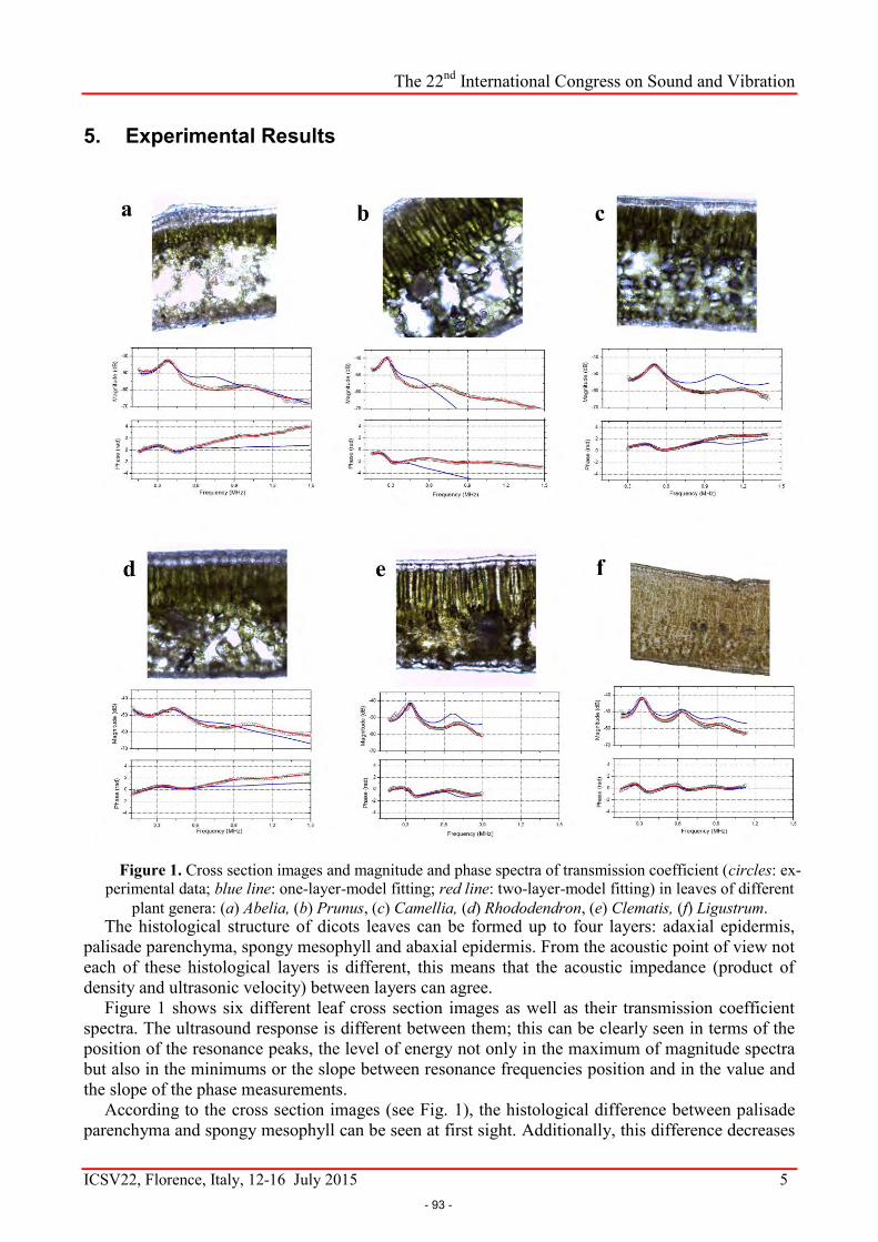
The 22nd International Congress on Sound and Vibration

ICSV22, Florence, Italy, 12-16 July 2015 5

5. Experimental Results

The histological structure of dicots leaves can be formed up to four layers: adaxial epidermis, palisade parenchyma, spongy mesophyll and abaxial epidermis. From the acoustic point of view not each of these histological layers is different, this means that the acoustic impedance (product of density and ultrasonic velocity) between layers can agree.

Figure 1 shows six different leaf cross section images as well as their transmission coefficient spectra. The ultrasound response is different between them; this can be clearly seen in terms of the position of the resonance peaks, the level of energy not only in the maximum of magnitude spectra but also in the minimums or the slope between resonance frequencies position and in the value and the slope of the phase measurements.

According to the cross section images (see Fig. 1), the histological difference between palisade parenchyma and spongy mesophyll can be seen at first sight. Additionally, this difference decreases

Figure 1. Cross section images and magnitude and phase spectra of transmission coefficient (circles: ex-perimental data; blue line: one-layer-model fitting; red line: two-layer-model fitting) in leaves of different

plant genera: (a) Abelia, (b) Prunus, (c) Camellia, (d) Rhododendron, (e) Clematis, (f) Ligustrum.

- 93 -

The 22nd International Congress on Sound and Vibration

ICSV22, Florence, Italy, 12-16 July 2015 6

from Abelia (a) to Ligustrum (f) in fact, Abelia leaves present a large and highly porous spongy mesophyll layer with very large pores, while in the Ligustrum leaves palisade parenchyma and spongy mesophyll are not so different and porosity of the spongy mesophyll is very low and pores much smaller. Due to this fact, the location of the first and second resonances in the transmission coefficient spectra shifts: while in Ligustrum (Fig.1.f) the position of the second peak is the double of the first one (as it was expected by the single layer model), in Abelia measurements (Fig.1.a.) the frequency of the second maximum of magnitude spectra is about three times the frequency of the first resonance, that is, the harmonic distortion is maximal in the Abelia leaves, where the differ-ences between the two layer of tissues are also maximal. This behaviour can be explain as follows: given the value of resonance frequency in every material characterized as a single layer the first peak is located at λ/2. This relation is given by the following equation:

(3)

In the particular case when the layer is attached to a plate made of another material, first reso-nance frequency of the lower impedance layer shifts to λ/4 while the resonance originated by the higher acoustic impedance keeps at λ/2. Due to the fact, that there is a tight link between the charac-

Table 1. Mean and standard deviation of acoustic properties of measured plant species classified by genus.

SPECIES ACOUSTIC

IMPEDANCE (MRayl)

SURFACE DENSITY

(kg/m2)

ATTENUATION (Np/m)

VELOCITY / THICKNESS

(MHz)

Abelia 0.864 ± 0.130 0.196 ± 0.015 28.8 ± 27.1 4.421 ± 0.732 0.119 ± 0.017 0.088 ± 0.012 18.7 ± 34 1.351 ± 0.047

Photinia 0.653 ± 0.127 0.214 ± 0.026 52.8 ± 30.6 3.079 ± 0.637 0.076 ± 0.019 0.059 ± 0.010 20.2 ± 3.2 1.270 ± 0.175

Prunus 0.544 ± 0.134 0.173 ± 0.035 62.1 ± 51.1 3.129 ± 3.155 0.079 ± 0.022 0.062 ± 0.013 15.2 ± 25.3 1.265 ± 1.334

Nerium 0.756 ± 0.075 0.245 ± 0.05 51.2 ± 11.7 3.155 ± 0.465 0.150 ± 0.013 0.113 ± 0.012 25.3 ± 3.4 1.334 ± 0.036

Camellia 0.864 ± 0.096 0.275 ± 0.040 15.4 ± 13.1 3.180 ± 0.469 0.199 ± 0.059 0.114 ± 0.035 12.3 ± 2.2 1.761 ± 0.144

Citrus 0.704 ± 0.057 0.197 ± 0.023 18.9 ± 11.9 3.635 ± 0.623 0.122 ± 0.031 0.064 ± 0.018 17.8 ± 1.2 1.935 ± 0.096

Viburnum 0.587 ± 0.084 0.167 ± 0.025 22.0 ± 14.1 3.588 ± 0.821 0.140 ± 0.036 0.078 ± 0.024 15.6 ± 4.7 1.856 ± 0.419

Rhododendron 0.571 ± 0.106 0.172 ± 0.047 42.9 ± 28.2 3.452 ± 0.685 0.133 ± 0.052 0.087 ± 0.039 25.9 ± 4.9 1.578 ± 0.171

Acer 0.494 ± 0.132 0.148 ± 0.049 374.9 ± 24.06 3.749 ± 2.406 0.147 ± 0.051 0.071 ± 0.026 211.5 ± 24.9 2.115 ± 0.249

Bougainvillea 0.353 ± 0.041 0.216 ± 0.055 0.298 ± 11.7 1.690 ± 0.316 0.109 ± 0.044 0.093 ± 0.044 15.1 ± 4.4 1.206 ± 0.115

Clematis 0.442 ± 0.066 0.294 ± 0.059 30.9 ± 14.6 1.517 ± 0.146 0.175 ± 0.051 0.163 ± 0.060 13.0 ± 2.6 1.108 ± 0.152

Ligustrum 0.419 ± 0.081 0.525 ± 0.198 12.8 ± 7.3 1.403 ± 0.654 0.239 ± 0.077 0.156 ± 0.061 12.2 ± 2.6 1.119 ± 0.139

- 94 -

The 22nd International Congress on Sound and Vibration

ICSV22, Florence, Italy, 12-16 July 2015 7

teristics of the cells forming every different biological tissue in the leaf and their mechanical re-sponse, we can assert that as consequence, there is also a direct relationship between the distortion of the frequency pattern measured respect to the theoretical one layer model and how acoustically different are the constituent layers of the leaf.

Significant parameters were worked out applying the layered model for every plant species measurements. More than 10 different measurements of each species were taken. The ultrasound parameters obtained were classified according to the 12 different genera measured. Results suggest that the resonances are very sensitive to leaf microstructure (see Fariñas et al., 2013 and 2014b), as a consequence of the wide range of different leaf morphologies considered within each genus, high values of standard deviation are shown in Table 1.

According to the behavior of the layered structure of the leaf commented above, the measured ratio of the acoustic impedances of the two layers in Abelia leaves (see Table 1) is up to 10 while the range of this ratio obtained for Ligustrum leaves begins about 1. At the same time, values of attenuation and velocity and thickness ratio in each forming layer are similar, revealing that in the particular case of Ligustrum, the acoustic behavior can be explained as a single layer (which can be also seen in the transmission coefficient plotted in Fig.1).

Attenuation coefficient values are typical of porous materials (see Álvarez-Arenas, 2003b), how-ever, it may appear strange that obtained values are larger in the palisade parenchyma than in the porous spongy mesophyll, where scattering effects must be significant. The reason for this behav-iour can be that in the palisade parenchyma layer, the cell walls act as wave guide, and ultrasound propagation takes place preferentially along this path. However, as the cell wall only occupies a small volume fraction (φ), wave amplitude is reduced in the same proportion, so there is a large apparent energy loss due to this effect, and this is taken into account by the model as if it were due to the attenuation coefficient:

(4)

Finally, the values of surface density shown in Table 1 are typical of leaves. This parameter indi-cates the distribution of mass between the considered layers. In case of Abelia leaves, the surface density ratio between layers is lower than the one observed in acoustic impedances. According to the optical image (Fig.1.a) this can be explained in terms of the palisade parenchyma, which is much thinner than the spongy mesophyll. On the contrary, in Ligustrum leaves the surface density ratio between layers is higher: palisade parenchyma (densely packed cells) in this case is thicker than spongy mesophyll one (high porosity).

6. ConclusionsAn acoustic layered model for plant leaves was proposed in this work. The validity of this model

was tested with experimental data coming from up to 12 different dicot leaf genera collected for this purpose. In order to make the selection, the histological differences between different layers form-ing the tissue of the plant leaves were taken into account.

Considering the one-layer-model, which assumes the whole leaf as a homogenous plate, effec-tive parameters can be obtained: density, thickness, ultrasound velocity and attenuation. The layered model proposed mainly comprises two layers for the species under study: one accounts for the pali-sade parenchyma and the upper epidermis, while the other one corresponds to the spongy mesophyll and the lower epidermis. From a mechanical point of view, there is a link between the form, rigidity and density of cells on each layer and the acoustic impedance of the material.

- 95 -

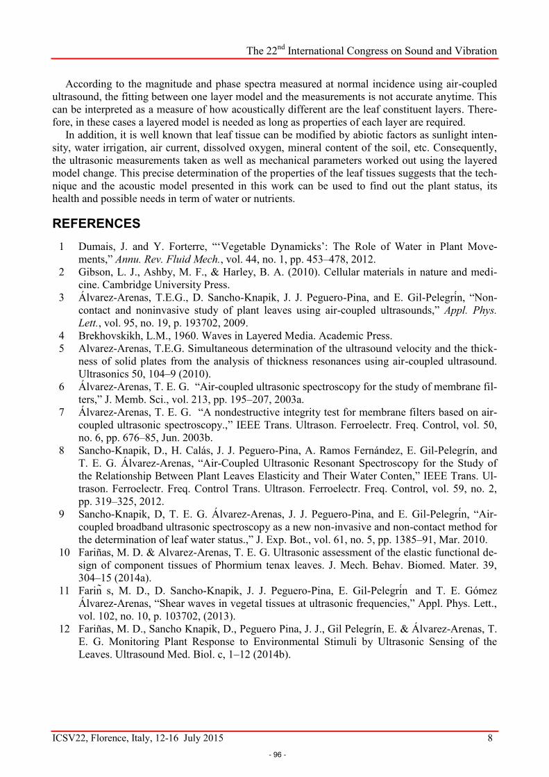
The 22nd International Congress on Sound and Vibration

ICSV22, Florence, Italy, 12-16 July 2015 8

According to the magnitude and phase spectra measured at normal incidence using air-coupled ultrasound, the fitting between one layer model and the measurements is not accurate anytime. This can be interpreted as a measure of how acoustically different are the leaf constituent layers. There-fore, in these cases a layered model is needed as long as properties of each layer are required.

In addition, it is well known that leaf tissue can be modified by abiotic factors as sunlight inten-sity, water irrigation, air current, dissolved oxygen, mineral content of the soil, etc. Consequently, the ultrasonic measurements taken as well as mechanical parameters worked out using the layered model change. This precise determination of the properties of the leaf tissues suggests that the tech-nique and the acoustic model presented in this work can be used to find out the plant status, its health and possible needs in term of water or nutrients.

REFERENCES 1 Dumais, J. and Y. Forterre, “‘Vegetable Dynamicks’: The Role of Water in Plant Move-

ments,” Annu. Rev. Fluid Mech., vol. 44, no. 1, pp. 453–478, 2012. 2 Gibson, L. J., Ashby, M. F., & Harley, B. A. (2010). Cellular materials in nature and medi-

cine. Cambridge University Press. 3 Álvarez-Arenas, T.E.G., D. Sancho-Knapik, J. J. Peguero-Pina, and E. Gil-Pelegrin, “Non-

contact and noninvasive study of plant leaves using air-coupled ultrasounds,” Appl. Phys. Lett., vol. 95, no. 19, p. 193702, 2009.

4 Brekhovskikh, L.M., 1960. Waves in Layered Media. Academic Press. 5 Alvarez-Arenas, T.E.G. Simultaneous determination of the ultrasound velocity and the thick-

ness of solid plates from the analysis of thickness resonances using air-coupled ultrasound. Ultrasonics 50, 104–9 (2010).

6 Álvarez-Arenas, T. E. G. “Air-coupled ultrasonic spectroscopy for the study of membrane fil-ters,” J. Memb. Sci., vol. 213, pp. 195–207, 2003a.

7 Álvarez-Arenas, T. E. G. “A nondestructive integrity test for membrane filters based on air-coupled ultrasonic spectroscopy.,” IEEE Trans. Ultrason. Ferroelectr. Freq. Control, vol. 50, no. 6, pp. 676–85, Jun. 2003b.

8 Sancho-Knapik, D., H. Calás, J. J. Peguero-Pina, A. Ramos Fernández, E. Gil-Pelegrín, and T. E. G. Álvarez-Arenas, “Air-Coupled Ultrasonic Resonant Spectroscopy for the Study of the Relationship Between Plant Leaves Elasticity and Their Water Conten,” IEEE Trans. Ul-trason. Ferroelectr. Freq. Control Trans. Ultrason. Ferroelectr. Freq. Control, vol. 59, no. 2, pp. 319–325, 2012.

9 Sancho-Knapik, D, T. E. G. Álvarez-Arenas, J. J. Peguero-Pina, and E. Gil-Pelegrin, “Air-coupled broadband ultrasonic spectroscopy as a new non-invasive and non-contact method for the determination of leaf water status.,” J. Exp. Bot., vol. 61, no. 5, pp. 1385–91, Mar. 2010.

10 Fariñas, M. D. & Alvarez-Arenas, T. E. G. Ultrasonic assessment of the elastic functional de-sign of component tissues of Phormium tenax leaves. J. Mech. Behav. Biomed. Mater. 39, 304–15 (2014a).

11 Farin s, M. D., D. Sancho-Knapik, J. J. Peguero-Pina, E. Gil-Pelegrin and T. E. Gómez Álvarez-Arenas, “Shear waves in vegetal tissues at ultrasonic frequencies,” Appl. Phys. Lett., vol. 102, no. 10, p. 103702, (2013).

12 Fariñas, M. D., Sancho Knapik, D., Peguero Pina, J. J., Gil Pelegrín, E. & Álvarez-Arenas, T. E. G. Monitoring Plant Response to Environmental Stimuli by Ultrasonic Sensing of the Leaves. Ultrasound Med. Biol. c, 1–12 (2014b).

- 96 -

1

Layer decomposition of bilayer composites using non-contact

resonant ultrasonic spectroscopy: application to soft polymers,

foams and plant tissues.

M.D. Fariñas, T.E.G. Álvarez-Arenas

Institute for Information and Physical Technologies (ITEFI), Spanish National Research Council

(CSIC), Serrano 144, 28006, Madrid

Abstract:

A procedure to extract some properties of the component layers of bilayer composites is

presented. The main target are dicot plant leaves, which show a layered structure with up to

four layers, although a simplified "acoustic two-layers model" can be a realistic approach. The

procedure employs a non-contact resonant ultrasonic spectroscopy technique to measure the

transmission coefficient spectra where several thickness resonances must be observed. An

ideal bilayer acoustic model and a stochastic gradient descent algorithm are used to calculate

the transmission coefficient and to solve the inverse problem. The problem of non-unique

solutions is discussed and dealt with by imposing some additional constrains that requires

some extra information about thickness and density ratios. Firstly, the technique is tested on

bilayers made of well known layers (rigid and soft polymers); comparison of extracted

properties with actual properties enables us to validate the procedure and to determine its

limitations. Then, it was applied to plant leaves of different species. In this case, some

information about the different layers of tissue is available from cross-section micrographs.

Differences in the extracted parameters of the different layers can be explained in terms of the

differences observed in the micrographs. Finally, elastic constants of each layer of tissue are

also worked out and a simple hexagonal cell model (consistent with microscopic observations)

is used to explain the differences observed in the elastic constants of palisade parenchyma and

spongy mesophyll tissues.

Keywords: Ultrasonic resonant spectroscopy, air-coupled ultrasound, layered composites,

bilayer, plant leaves, inverse problem.

- 97 -

2

1. Introduction

Layered composite materials are widespread in nature. Examples are found in nacre,

wood,1,2 plant leaves, wood and bamboo,3,4 gastrointestinal walls, skulls,5,6 tendons, skin,7

bones and cartilages.8,9 Many times, a hierarchical organization is also found in these materials

where properties vary at different levels of microstructure with highly interactions between

them.10,11 Therefore, macroscopic properties cannot be inferred from microscopic details, but

from the organization and properties at the mesoscopic level. Functional design in layered and

hierarchical materials implies that each layer/scale fulfills one function with the minimum side

effects on the others.12 This organization both functional and hierarchical makes possible to

meet a complex and wide spectrum of requirements and functions. In plant leaves, which

inspired this work, different layers with different functions can be distinguished along with the

vascular system, the most common layers are i) the Palisade Parenchyma (PP): a dense pack of

elongated cells oriented normal to the leaf plane, closely linked to interaction with light, ii) the

Spongy Mesophyll (SM): a porous layer with interconnected (open-pore) porosity where

gaseous interchange takes place and iii) Epidermis layers (that includes stomata and

trichomes): a thin layer that act as a barrier and control the leaf water loss through

evaporation. Different length scales are also involved; they range from the microscopic

composite structure of the cell wall,13 to the mesoscopic level including cell shape and size and

cell organization to form the different tissues.

Resonant ultrasonic spectroscopy (RUS)14-16 is a well know technique that permit to obtain

the elastic constants of solid materials from samples having a well defined geometry from the

analysis of the resonant frequencies of the different modes of vibration. In the case of plates,

air-coupled ultrasound has been used to excite and sense thickness resonances and hence, to

obtain elastic constants.17-19 In this sense this technique can be denominated as non-contact

RUS, although there are some significant differences between both techniques. Unlike in

conventional RUS, in this case we have a one-dimensional problem and the full transmission

coefficient spectra, where the air-load is considered, is considered to solve the inverse

problem (and not only the frequency location of the resonances). Finally, in non-contact RUS

applied to layered tissues, resonances appear at relatively higher frequencies and because of

the materials considered here (that present a very large attenuation coefficient), the number

of resonances that can be observed is limited.

Three main conclusions have been derived from previous studies of plant leaves using

non-contact or air-coupled RUS in the vicinity of the first order thickness resonance. First, that

a simple one-layer model20 can be used to extract effective material properties; second, that

- 98 -

3

these extracted properties agree well with measurements obtained by alternative methods;21

and third, that these extracted properties provide meaningful ecophysiological information,

specially about plant water relations.22 This ultrasonic technique combines high frequency (0.1

– 1.5 MHz), large wavelength (typically > 200 m) and very small displacements ( < 100 nm).

Hence, the applied stress and deformation fields can be considered homogeneous over the

cellular length scale, the cell deformation is small compared with the cell size and can be

considered, in most of the cases, within the linear regime and cell deformation takes place

without changing the cell fluid content as the fluid flow relaxation time are much longer that

wave period.23 These features cannot be achieved by other techniques (Pressure chamber,

indentation and mechanical tests, AFM techniques, etc.), where the cell deformation can be

very large, the time scale comparable to the fluid flow (across cell wall) relaxation time and

stress and/or deformation is not homogeneous over the cell volume.

Further expansion of the frequency span in order to observe two or more orders of the

leaf thickness resonances presents a strong potential to study the leaf viscoelasticity.24

However, a significant distortion, compared with the one-layer predictions, has been

observed.21,25 It has been suggested that this is due to the layered structure of the plant leaves;

but we are still far from being able to extract layers properties as we have done in the past

with the one layer model.

This paper focuses on the extraction of the properties of the layers of bilayer composite

plates from the measurement of the magnitude and phase spectra of the transmission

coefficient (TC). This is called layer decomposition. We focus on bilayers because this is the

simplest layered structure, it is also the basic structure some other more complex layered

materials are made of and an acoustic two-layers model has already been proposed for dicot

leaves based on the leaf anatomy, where one of the layers of this acoustic model corresponds

to the epidermis + PP and the other one in SM + epidermis.26 Furthermore the proposed

procedure has the potential to be applied to more complex layered composites like sandwich

structures27 and stacks of bilayers by changing the way the initial guess is obtained and

adapting the set of constrains.

2. Ultrasound transmission through layered media

Wave propagation in multilayered materials has been studied before by many authors28

and resonant techniques in layered materials have been largely used to obtain materials

properties.17,29,30, For a single plate of acoustic impedance Zp, placed between two media with

impedances Z1 and Z2, thickness resonances appear in the transmission coefficient spectra (TC)

- 99 -

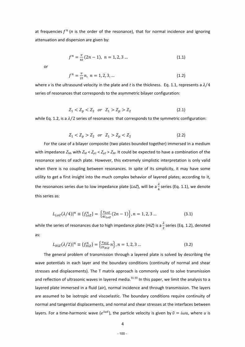
4

at frequencies 𝑓𝑛 (n is the order of the resonance), that for normal incidence and ignoring

attenuation and dispersion are given by:

𝑓𝑛 =𝑣

4𝑡(2𝑛 − 1), 𝑛 = 1, 2, 3 … (1.1)

or

𝑓𝑛 =𝑣

2𝑡𝑛, 𝑛 = 1, 2, 3, … (1.2)

where v is the ultrasound velocity in the plate and t is the thickness. Eq. 1.1, represents a 𝜆 4⁄

series of resonances that corresponds to the asymmetric bilayer configuration:

𝑍1 < 𝑍𝑝 < 𝑍2 𝑜𝑟 𝑍1 > 𝑍𝑝 > 𝑍2 (2.1)

while Eq. 1.2, is a 𝜆 2⁄ series of resonances that corresponds to the symmetric configuration:

𝑍1 < 𝑍𝑝 > 𝑍2 𝑜𝑟 𝑍1 > 𝑍𝑝 < 𝑍2 (2.2)

For the case of a bilayer composite (two plates bounded together) immersed in a medium

with impedance ZM, with ZM < Zp1 < Zp2 > ZM. It could be expected to have a combination of the

resonance series of each plate. However, this extremely simplistic interpretation is only valid

when there is no coupling between resonances. In spite of its simplicity, it may have some

utility to get a first insight into the much complex behavior of layered plates; according to it,

the resonances series due to low impedance plate (LoZ), will be a 𝜆

4 series (Eq. 1.1), we denote

this series as:

𝐿𝐿𝑜𝑍(𝜆 4⁄ )|𝑛 ≡ {𝑓𝐿𝑜𝑍𝑛 } = {

𝑣𝐿𝑜𝑍

4𝑡𝐿𝑜𝑍(2𝑛 − 1)} , 𝑛 = 1, 2, 3 … (3.1)

while the series of resonances due to high impedance plate (HiZ) is a 𝜆

2 series (Eq. 1.2), denoted

as:

𝐿𝐻𝑖𝑍(𝜆 2⁄ )|𝑛 ≡ {𝑓𝐻𝑖𝑍𝑛 } = {

𝑣𝐻𝑖𝑍

2𝑡𝐻𝑖𝑍𝑛} , 𝑛 = 1, 2, 3 … (3.2)

The general problem of transmission through a layered plate is solved by describing the

wave potentials in each layer and the boundary conditions (continuity of normal and shear

stresses and displacements). The T matrix approach is commonly used to solve transmission

and reflection of ultrasonic waves in layered media.31-33 In this paper, we limit the analysis to a

layered plate immersed in a fluid (air), normal incidence and through transmission. The layers

are assumed to be isotropic and viscoelastic. The boundary conditions require continuity of

normal and tangential displacements, and normal and shear stresses at the interfaces between

layers. For a time-harmonic wave (𝑒𝑖𝜔𝑡), the particle velocity is given by �� = 𝑖𝜔𝑢, where u is

- 100 -

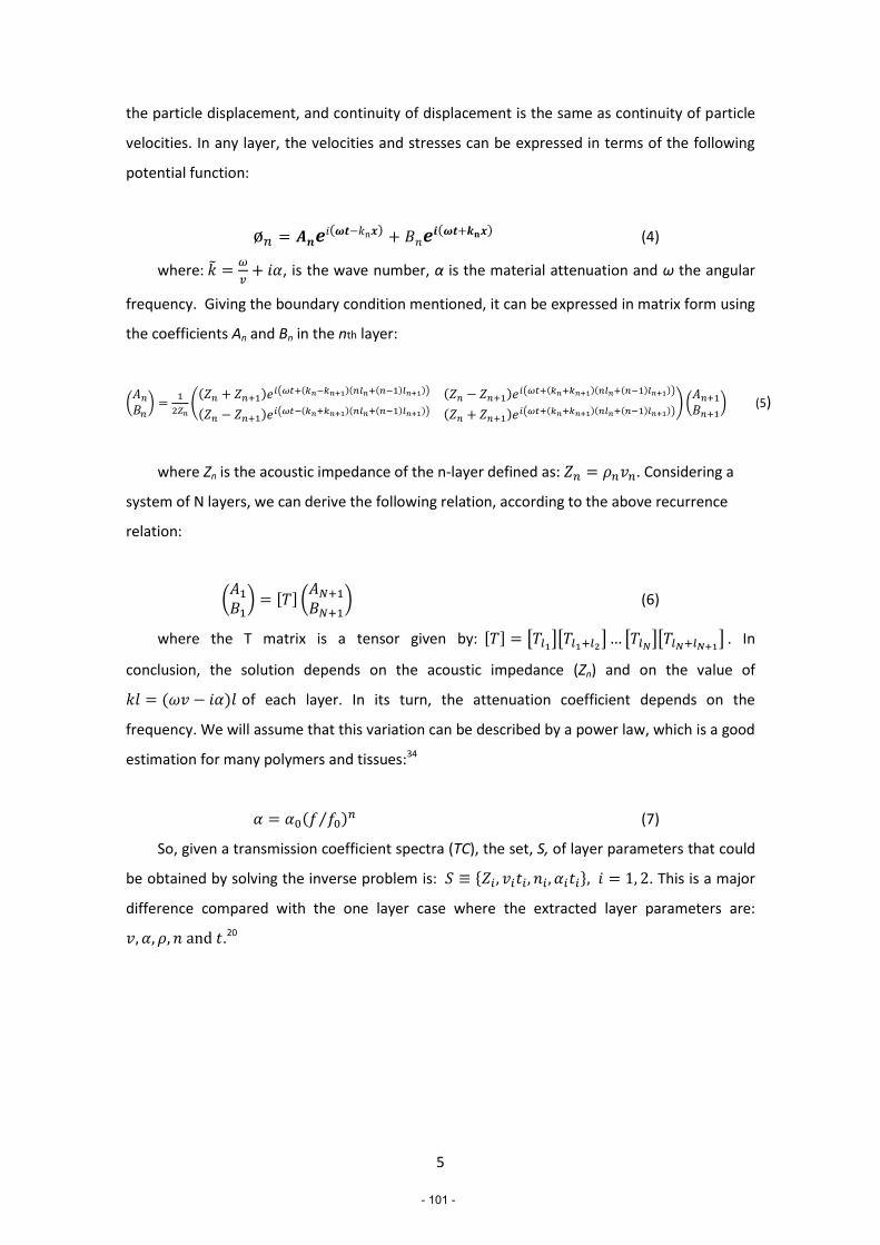
5

the particle displacement, and continuity of displacement is the same as continuity of particle

velocities. In any layer, the velocities and stresses can be expressed in terms of the following

potential function:

ø𝑛 = 𝑨𝒏𝒆𝑖(𝝎𝒕−𝑘n𝒙) + 𝐵𝑛𝒆𝒊(𝝎𝒕+𝒌𝐧𝒙) (4)

where: �� =𝜔

𝑣+ 𝑖𝛼, is the wave number, α is the material attenuation and ω the angular

frequency. Giving the boundary condition mentioned, it can be expressed in matrix form using

the coefficients An and Bn in the nth layer:

(𝐴𝑛

𝐵𝑛) =

1

2𝑍𝑛(

(𝑍𝑛 + 𝑍𝑛+1)𝑒𝑖(𝜔𝑡+(𝑘𝑛−𝑘𝑛+1)(𝑛𝑙𝑛+(𝑛−1)𝑙𝑛+1)) (𝑍𝑛 − 𝑍𝑛+1)𝑒𝑖(𝜔𝑡+(𝑘𝑛+𝑘𝑛+1)(𝑛𝑙𝑛+(𝑛−1)𝑙𝑛+1))

(𝑍𝑛 − 𝑍𝑛+1)𝑒𝑖(𝜔𝑡−(𝑘𝑛+𝑘𝑛+1)(𝑛𝑙𝑛+(𝑛−1)𝑙𝑛+1)) (𝑍𝑛 + 𝑍𝑛+1)𝑒𝑖(𝜔𝑡+(𝑘𝑛+𝑘𝑛+1)(𝑛𝑙𝑛+(𝑛−1)𝑙𝑛+1))) (

𝐴𝑛+1

𝐵𝑛+1) (5)

where Zn is the acoustic impedance of the n-layer defined as: 𝑍𝑛 = 𝜌𝑛𝑣𝑛. Considering a

system of N layers, we can derive the following relation, according to the above recurrence

relation:

(𝐴1

𝐵1) = [𝑇] (

𝐴𝑁+1

𝐵𝑁+1) (6)

where the T matrix is a tensor given by: [𝑇] = [𝑇𝑙1][𝑇𝑙1+𝑙2

] … [𝑇𝑙𝑁][𝑇𝑙𝑁+𝑙𝑁+1

] . In

conclusion, the solution depends on the acoustic impedance (Zn) and on the value of

𝑘𝑙 = (𝜔𝑣 − 𝑖𝛼)𝑙 of each layer. In its turn, the attenuation coefficient depends on the

frequency. We will assume that this variation can be described by a power law, which is a good

estimation for many polymers and tissues:34

𝛼 = 𝛼0(𝑓 𝑓0⁄ )𝑛 (7)

So, given a transmission coefficient spectra (TC), the set, S, of layer parameters that could

be obtained by solving the inverse problem is: 𝑆 ≡ {𝑍𝑖, 𝑣𝑖𝑡𝑖, 𝑛𝑖, 𝛼𝑖𝑡𝑖}, 𝑖 = 1, 2. This is a major

difference compared with the one layer case where the extracted layer parameters are:

𝑣, 𝛼, 𝜌, 𝑛 and 𝑡.20

- 101 -

6

3. Layer decomposition of bilayer composites from the

analysis of thickness resonances in the transmission coefficient

spectra.

In section 2 we have seen that given the set of layer parameters S: 𝑆 ≡ {𝑥𝑖} =

{𝑍𝑖 , 𝑣𝑖𝑡𝑖, 𝑛𝑖, 𝛼𝑖𝑡𝑖}, 𝑖 = 1,2 and a frequency vector {𝑓𝑘}, TC can be theoretically calculated. Let

us suppose now, that we have a digitized target spectra (TS) defined as the magnitude and

phase spectra of the TC of a bilayer (TS can be either measured or computer generated), given

by:

𝑇𝑆 = [ {𝑓𝑘}, {|𝑇𝐶(𝑓𝑘)| }, {𝜙(𝑇𝐶(𝑓𝑘))} ] (8),

where:

𝑓𝑘 = {𝑓1, 𝑓2, … 𝑓𝑁} ≡ 𝑑𝑖𝑔𝑖𝑡𝑖𝑧𝑒𝑑 𝑓𝑟𝑒𝑞𝑢𝑒𝑛𝑐𝑦 𝑣𝑒𝑐𝑡𝑜𝑟 (9),

|𝑇𝐶(𝑓𝑘)| ≡ 𝑀𝑎𝑔𝑛𝑖𝑡𝑢𝑑𝑒 𝑠𝑝𝑒𝑐𝑡𝑟𝑢𝑚 (10),

𝜙(𝑇𝐶(𝑓𝑘)) ≡ 𝑃ℎ𝑎𝑠𝑒 𝑠𝑝𝑒𝑐𝑡𝑟𝑢𝑚 (11)

Given a TS, we want to perform the layer decomposition which is equivalent to solve

the inverse problem, that is, to find the set of layer parameters 𝑆 that minimizes the error ()

between the calculated spectra (TCcalc) and TS. Error 휀 is given by:

휀 = 휀(𝑇𝐶(𝑆)𝑐𝑎𝑙𝑐 , 𝑇𝑆) = √휀𝑚𝑎𝑔2 + 휀𝑝ℎ𝑎𝑠𝑒

2 (12),

where

휀𝑚𝑎𝑔 = 휀𝑚𝑎𝑔(𝑇𝐶(𝑆)𝑐𝑎𝑙𝑐 , 𝑇𝑆) = √∑(|𝑇𝐶(𝑆,𝑓𝑖)|𝑐𝑎𝑙𝑐−|𝑇𝑆(𝑓𝑖)| )2

𝑁(13.1),

휀𝑝ℎ𝑎𝑠𝑒 = 휀𝑝ℎ𝑎𝑠𝑒(𝑇𝐶(𝑆)𝑐𝑎𝑙𝑐, 𝑇𝑆) =√∑(𝜙(𝑇𝐶(𝑆,𝑓𝑖))

𝑐𝑎𝑙𝑐− 𝜙( 𝑇𝑆(𝑓𝑖)))

2

𝑁(13.2)

Let 𝑆0 be the solution of the layer decomposition problem of a given TS, that is:

휀𝑚𝑖𝑛 = 휀(𝑇𝐶(𝑆0)𝑐𝑎𝑙𝑐 , 𝑇𝑆), we define the set of k-different layer decompositions: 𝐼𝑆(𝑇𝑆, ∆) =

{𝑆𝑗}, 𝑗 = 1, 2, … , 𝑘 as the set that fulfills:

∀ 𝑆𝑗 ∈ 𝐼𝑆(𝑇𝑆, ∆) ⟺ 휀 (𝑇𝐶(𝑆𝑗)𝑐𝑎𝑙𝑐

, 𝑇𝑆) ≤ 휀𝑚𝑖𝑛 + ∆ (14.1)

We call 𝐼𝑆(𝑇𝑆, ∆) the set of k-different indistinguishable layer decompositions within ∆, if

∆> 0, then 𝑘 ≥ 1.

- 102 -

7

The main difficulties to solve this inverse problem are 𝑘 > 1 and the high dimension of

the space of search (8 variables). The dimension of the space of search makes impractical the

use of a systematic search so local search methods are preferred, however use of local search

methods makes necessary to implement a way to deal with local minima within the problem

domain.35 The way to deal with these problems is to set constrains, to get an initial guess as

close as possible to the physical solution of interest and to divide the problem domain in

several sub domains.

Initial guess First, the portion of TS in the vicinity of the first thickness resonance (-6dB frequency

window: TS6dB) is only considered and effective parameters (𝑆06𝑑𝐵 = {𝑡𝑒𝑓𝑓

𝑢𝑠 , 𝜌𝑒𝑓𝑓𝑢𝑠 , 𝑣𝑒𝑓𝑓

𝑢𝑠 , 𝛼𝑒𝑓𝑓𝑢𝑠 })

thickness, density, ultrasonic velocity and attenuation coefficient at the resonant frequency

are extracted.20,36 As we know that, at least for plant leaves, 𝑡𝑒𝑓𝑓𝑢𝑠 , 𝜌𝑒𝑓𝑓

𝑢𝑠 and 𝑣𝑒𝑓𝑓𝑢𝑠 are in good

agreement with direct measurements of these parameters,21 the idea is to use 𝑆06𝑑𝐵 to

generate the initial guess. Nonetheless and to further check how close is 𝑆06𝑑𝐵 to the actual

effective properties of bilayer composites whose properties may differ from that of plant

leaves, we generated 75 different bilayer configurations, for each bilayer we generated TS6dB,

extracted 𝑆06𝑑𝐵, then calculated effective properties (𝑆0) (Eqs. 15), and finally compared 𝑆0 and

𝑆06𝑑𝐵.

𝑡𝑒𝑓𝑓 = 𝑡1 + 𝑡2 (15.1)

𝜌𝑒𝑓𝑓 = (𝑡1𝜌1 + 𝑡2𝜌2) 𝑡𝑒𝑓𝑓⁄ (15.2)

𝑣𝑒𝑓𝑓 = 𝑡𝑒𝑓𝑓 (𝑡1 𝑣1⁄ + 𝑡2 𝑣2⁄ )⁄ (15.3)

𝛼𝑒𝑓𝑓 = (𝑡1𝛼1 + 𝑡2𝛼2) 𝑡𝑒𝑓𝑓⁄ (15.4)

where subindex 1 and 2 refers to layers 1 and 2.

Let us denote the high and low impedance layers as HiZ and LoZ, respectively; to generate

the 75 different bilayer composites we proceed as follows: in all cases, (𝑣 𝑡⁄ )𝐿𝑜𝑍 = 1 𝑀𝐻𝑧,

and three different values of 𝑍𝐿𝑜𝑍 have been considered: 0.2, 0.4 and 0.8 MRayl. Then five

different ratios (𝑣 𝑡⁄ )𝐻𝑖𝑍 (𝑣 𝑡⁄ )𝐿𝑜𝑍⁄ : 1.0, 1.5, 2.0, 2.5, 3.0 and five 𝑍𝐻𝑖𝑍 𝑍𝐿𝑜𝑍⁄ ratios: 1.25, 2.50,

3.75, 5.00, 6.25, were considered. In addition, 𝛼𝐻𝑖𝑍 = 𝛼𝐿𝑜𝑍 = 170 Np/m at 100 kHz,

𝑛𝐻𝑖𝑍 = 𝑛𝐿𝑜𝑍 =1, external medium was air and only normal incidence was considered. Best

agreement is obtained for effective thickness and velocity; in this case,

|𝑡𝑒𝑓𝑓𝑢𝑠 − 𝑡𝑒𝑓𝑓| 𝑡𝑒𝑓𝑓 ≤ 0.1⁄ , |𝑣𝑒𝑓𝑓

𝑢𝑠 − 𝑣𝑒𝑓𝑓| 𝑣𝑒𝑓𝑓 ≤ 0.1⁄ . Effective density and attenuation

present a much more heterogeneous behavior |𝜌𝑒𝑓𝑓𝑢𝑠 − 𝜌𝑒𝑓𝑓| 𝜌𝑒𝑓𝑓 ≤ 0.3⁄ ,

- 103 -

8

|𝛼𝑒𝑓𝑓𝑢𝑠 − 𝛼𝑒𝑓𝑓| 𝛼𝑒𝑓𝑓 ≤ 0.3⁄ where the general trend is that error increases as the two layers

become more different.

To generate the initial guess from 𝑆06𝑑𝐵 we have used two other input data: 𝑟𝑡 =

𝑡𝐻𝑖𝑍 𝑡𝐿𝑜𝑍⁄ and 𝑟𝜌 = 𝜌𝐻𝑖𝑍 𝜌𝐿𝑜𝑍⁄ . The rationale for this choice is explained in next section. In

addition, we assume that the first observed resonance (𝑓𝑟𝑒𝑠0 ) corresponds to the first /4

resonance of the LoZ layer, that the second one (𝑓𝑟𝑒𝑠1 ) corresponds to the first /2 resonance

of the HiZ layer, that attenuation is the same in both layers and equal to 𝛼𝑒𝑓𝑓𝑢𝑠 , and n is equal to

1 in both layers:

𝑡𝐻𝑖𝑍 = 𝑟𝑡 𝑡𝑒𝑓𝑓𝑢𝑠 (1 + 𝑟𝑡)⁄ (16.1)

𝑡𝐿𝑜𝑍 = 𝑡𝑒𝑓𝑓𝑢𝑠 (1 + 𝑟𝑡)⁄ (16.2)

𝜌𝐻𝑖𝑍 = 𝑟𝜌 𝜌𝑒𝑓𝑓𝑢𝑠 (1 + 𝑟𝜌)⁄ (16.3)

𝜌𝐿𝑜𝑍 = 𝜌𝑒𝑓𝑓𝑢𝑠 (1 + 𝑟𝜌)⁄ (16.4)

𝑣𝐿𝑜𝑍 = 4𝑡𝐿𝑜𝑍𝑓𝑟𝑒𝑠0 (16.5)

𝑣𝐻𝑖𝑍 = 2𝑡𝐻𝑖𝑍𝑓𝑟𝑒𝑠1 (16.6)

𝛼𝐻𝑖𝑍 = 𝛼𝐿𝑜𝑍 = 𝛼𝑒𝑓𝑓𝑢𝑠 (16.7)

𝑛𝐻𝑖𝑍 = 𝑛𝐿𝑜𝑍 = 1.0 (16.8)

This very simplified version of the initial guess has the advantage that the required

previous information about the bilayer composite is reduced. If any other information about

the material is available, this initial guess could be improved and this will permit to further

reduce the computation complexity of the problem and the time of computation. Nonetheless,

for all the fittings shown in this work the initial guess was obtained in this way.

Constrains. A constrain is defined as a logical relation (a property that must be satisfied) among a set

of unknowns.37 The set of unknowns in our case is 𝑆 ≡ {𝑍𝑖 , 𝑣𝑖𝑡𝑖, 𝑛𝑖, 𝛼𝑖𝑡𝑖} , 𝑖 = 1,2, The

choice of constrains will largely depend on the particular application, frequency range, range

of materials properties and previous knowledge of the problem domain. The main objective of

the use of constrains in this case is to limit the space of search and to reduce the size of the set

of indistinguishable solutions (IS). Our experience fitting a large number of experimental and

computer generated TS using materials similar to those used in this paper has revealed that:

∀ 𝑆𝑗, 𝑆𝑘 ∈ 𝐼𝑆: {𝑣𝑖𝑡𝑖, 𝑛𝑖, 𝛼𝑖𝑡𝑖}𝑗 ≅ {𝑣𝑖𝑡𝑖, 𝑛𝑖, 𝛼𝑖𝑡𝑖}𝑘 , 𝑏𝑢𝑡 𝑍𝑖𝑗 ≠ 𝑍𝑖𝑘

, where i = 1, 2 and

𝑍1𝑗 𝑍2𝑗⁄ ≠ 𝑍1𝑘 𝑍2𝑘⁄ . That is, in order to effectively limit the IS set, we should have some

- 104 -

9

knowledge about 𝑍1 𝑍2⁄ . However imposing constrains on 𝑍1 𝑍2⁄ is not very efficient as

impedance is the product of ultrasound velocity and density and the range of variation can be

rather large. Alternatively, if ti can be fixed then the solution Sj is now given by: 𝑆𝑗 ≡

{𝑡𝑖, 𝜌𝑖, 𝑣𝑖 , 𝑛𝑖, 𝛼𝑖}𝑗, 𝑖 = 1,2 , and ∀ 𝑆𝑗, 𝑆𝑘 ∈ 𝐼𝑆: {𝑡𝑖, 𝑣𝑖, 𝑛𝑖 , 𝛼𝑖}𝑗 ≅ {𝑡𝑖, 𝑣𝑖, 𝑛𝑖, 𝛼𝑖}𝑗 , 𝑏𝑢𝑡 𝜌𝑖𝑗 ≠

𝜌𝑖𝑘, where i = 1, 2 and 𝜌1𝑗 𝜌2𝑗

⁄ ≠ 𝜌1𝑘 𝜌2𝑘⁄ . That is, in this case, constrains can be imposed

on 𝜌1 𝜌2⁄ , and this can much more precisely be done.

Imposing constrains on 𝜌1 𝜌2⁄ is actually a convenient solution for plant leaves as this

ratio (𝜌𝑃𝑃 𝜌𝑆𝑀⁄ ) is mainly determined by the porosity ratio of the PP and SM layers. Overall

leaf porosity is, normally, in the range 30-60%.38 In addition, porosity values or PP and SM

layers have already been reported by several authors, for Arabidopsis thaliana leaves,39 SM

and PP tissues porosity is about 55% and 25%, respectively,40 while for other species a range of

porosities 15%–30% and 25%–65%, for PP and SM, respectively, have been reported,41,42 these

data suggests: 1.07 < 𝜌𝑃𝑃 𝜌𝑆𝑀⁄ < 2.43.

In addition, cross-section images of leaves using fresh cuts and optical microscopy are

routinely taken where thickness and porosity of each layer can be determined. Therefore, this

is the selected approach in this work: constrains are imposed for the minimum and maximum

value of 𝑟𝜌, 𝑟𝑡 is taken from optical cross-sections and the total thickness is set equal to 𝑡𝑒𝑓𝑓𝑢𝑠 .

However keeping thicknesses fixed is a very restrictive constrain that easily turns the problem

overconstrained. Therefore, thicknesses are also used as fitting variables but their variation is

limited as shown in eqs. 17, where 𝛽 determines the allowed range of variation. In summary,

the thickness ratio is used as a soft constrain, while all the other constrains are hard. The full

set of constrains imposed are summarized in Eqs. 17 and Table I.

𝜌𝐻𝑖𝑍 𝜌𝐿𝑜𝑍 ∈ ⁄ [𝑟𝜌𝑚𝑖𝑛, 𝑟𝜌𝑚𝑎𝑥

] (17.1)

𝑟𝑡𝑡𝑒𝑓𝑓 (1 + 𝑟𝑡) × (1 − 𝛽)⁄ < 𝑡𝐻𝑖𝑍 < 𝑟𝑡𝑡𝑒𝑓𝑓 (1 + 𝑟𝑡) × (1 + 𝛽)⁄ (17.2)

𝑡𝑒𝑓𝑓 (1 + 𝑟𝑡) × (1 − 𝛽)⁄ < 𝑡𝐿𝑜𝑍 < 𝑡𝑒𝑓𝑓 (1 + 𝑟𝑡) × (1 + 𝛽)⁄ (17.3)

𝜌𝑖 ∈ [𝜌𝑖𝑚𝑖𝑛, 𝜌𝑖

𝑚𝑎𝑥], 𝑖 = 𝐻𝑖𝑍, 𝐿𝑜𝑍 (17.4)

0 < 𝑛𝑖 < 4, 𝑖 = 𝐻𝑖𝑍, 𝐿𝑜𝑍 (17.5)

𝛼𝑖 > 0, 𝑖 = 𝐻𝑖𝑍, 𝐿𝑜𝑍 (17.6)

Table I. Numerical values of constrains for synthetic bilayers and plant leaves.

Synthetic bilayers Plant tissues

LoZ HiZ LoZ HiZ

𝜌𝑚𝑖𝑛 (kg/m3) 250 400 150 600

𝜌𝑚𝑎𝑥 (kg/m3) 1700 1900 950 1150

- 105 -

10

𝑟𝜌𝑚𝑖𝑛0.85 1.1

𝑟𝜌𝑚𝑎𝑥3.0 3.1

𝛽 5% 10%

Fitting algorithm.

First, the interval [𝑟𝜌𝑚𝑖𝑛, 𝑟𝜌𝑚𝑎𝑥

], for Table I, is divided in 6 subintervals and the fitting

process explained below is repeated taking each of these subintervals as constrains, taking at

each step the value of 𝑟𝜌 for the initial guess (Eq. 16) as the centre value in each of these

intervals and keeping the limits of the subinterval as constrains. This permits us to detect the

presence of several local minima and to evaluate if they can be considered as indistinguishable

solutions.

The algorithm structure is the same one as the one described in36: two nested loops, the

first one varies 𝑡𝑖, 𝑣𝑖 and 𝜌𝑖, i = 1,2, for the two layers; while the second one varies 𝛼𝑖 and ni, i

= 1,2. In this case and in order to be able to cope with the larger dimension of the space of

search, a local search technique is used (in particular a Stochastic Gradient Descent –SGD-

technique) instead of the systematic search technique (or brute force approach) used before.36

Gradient descent or steepest descent methods are widely used in regression problems and

machine learning applications; they have also been used in the context of inverse problem

solution for resonant ultrasonic measurements. The SGD routine used in this case has been

implemented specifically for this problem, it is written in Python 2.7. For the results shown in

this paper, it has always been operated in either a six or four dimensions space as there are

two sets of parameters to optimize: {𝑥��}, 𝑖 = 1 − 4 𝑜𝑟 𝑖 1 − 6: {𝑥��} = {𝜌1, 𝜌2, 𝑣1, 𝑡1, 𝑣2, 𝑡2}

and {𝑥��} = {𝑛1, 𝑛2, 𝛼1, 𝛼2}. Given an estimation: {𝑥��}0, the discrete volume around {𝑥��}

0

determined by the points: {𝑥��(1 ± 𝛿)}, is searched for any set of values {𝑥��}′ that reduces .

In general, the number of points in this volume is given by: 𝑉 = 3𝑁, where N is the dimension

of the hyperspace {𝑥��}. Therefore, V increases very fast with N, and this is the main reason to

break the problem into two loops. For N = 4 and 6, V = 81 and 729, respectively, while for the

whole problem N = 10 and then V = 59049. Once the first {𝑥𝑖}′ is found we stop searching and

move along the direction given by the vector {𝑥��}′ − {𝑥��} a step of length equal to 2. The

process is repeated until either no further reduction in is found or the maximum number of

iterations allowed is reached, this maximum number of iterations is set to 10.

- 106 -

11

Figure 1. Schematic representation of the routine to extract layer parameters from TC magnitude

and phase spectra.

These two SGD loops are repeated while 휀𝑛 < 𝛾휀𝑛−1 where 휀𝑛 is the error 휀 (Eq. 15) after

the n-th iteration and 𝛾 = 0.999. The step size in the SGD () is kept constant: = 0.01. We will

call extracted parameters: {𝑥𝑖𝑒} ≡ {𝑡𝑖

𝑒 , 𝑣𝑖𝑒 , 𝜌𝑖

𝑒 , 𝛼𝑖𝑒 , 𝑛𝑖

𝑒 }, 𝑖 = 1, 2 to the set of parameters {𝑥𝑖}

obtained at the end of this process. After repeating the process for all the subintervals in

[𝑟𝜌𝑚𝑖𝑛, 𝑟𝜌𝑚𝑎𝑥

], we can take all {𝑥𝑖𝑒}𝑗 ∈ 𝐼𝑆(𝑇𝑆, ∆) and get a mean value and standard deviation

of the extracted parameters: mean({𝑥𝑖𝑒}) and std({𝑥𝑖

𝑒}). Results shown are obtained with

∆ = 5%.

4. Materials

a. Polymeric plates

Eleven different synthetic bilayer composites (see Table II) have been studied. Sorted as

hard and soft bilayers (A-C and D-G, respectively), they were fabricated by attaching together a

high and a low impedance layer (Hi-Z and Lo-Z) using either ultrasonic gel coupling (for hard

bilayers) or a 50 µm pressure sensitive double sided adhesive tape (soft bilayers). Plate sizes

were, typically, 60 mm x 60 mm and measurements were repeated several times at different

points over the plate surface to get averaged values and standard deviations. We will refer to

the set of values of a given bilayer: {𝑥𝑖∗} ≡ {𝑡𝑖

∗, 𝑣𝑖∗, 𝜌𝑖

∗, 𝛼𝑖∗, 𝑛𝑖

∗ }, 𝑖 = 1, 2 as the expected values.

Table II. Composition of the synthetic bilayers fabricated and properties of the employed plates

(mean values and standard deviations).

Type Bilayer Material Thickness Velocity Density α @ fo n fo

- 107 -

12

(µm) (m/s) (kg/m3) (Np/m) (kHz)

Lo-Z

A, A2 Elastomer 939 0.07

899.3 83.6

1340.5 99.9

24.49 1.83

0.6 0.1

477.9 8.9

B, C Elastomer 1049 0.08

1006.4 95.8

916.4 69.88

31.5 2.4

0.3 0.1

478.75 9.1

D, E, E2,

F, F2 PP foam

92 0.005

118.0 8.0

372.3 20.2

2144 116.5

1.8 0.1

640.1 8.69

G, G2 PS foam 132

0.005 218.8 10.2

411.2 15.6

802.1 30.4

0.9 0.1

821.8 7.78

Hi-Z

A Rubber-1 2037 0.08 1635.0

79.82 1472.2

72.3

42.3 1.67 0.7

0.1

399.1 3.91

A2 Rubber-2 1018 0.05

68.5 2.1

199.2 2.4

B PU 3140 0.08

1837.0 117.1

1053.0 26.8

75.78 1.93

0.9 0.1

292.5 3.72

C CFRP 4398 0.08

2740.0 62.4

1649.0 29.6

15.1 0.27

1.0 0.1

310.2 1.41

D PU-foam-1 1270 0.08

1525.0 120.2

644.0 40.45

100.2 6.3

0.5 0.1

600.1 9.45

E PU-foam-2 1020 0.06 1481.2

109.8 654.0 41.8

133.4 7.8 0.6

0.1

732.2 10.7

E2 PU-foam-3 617 0.04

192.8 8.6

439.2 7.1

F, G Cellulose-1 226

0.008 696.9 30.4

1093.9 38.7

2090.9 74.0

n.a.

1520.1 13.4

F2, G2 Cellulose-2 303 0.01

1580.0 52.1

1140.5 9.4

b. Biological tissues: Plant Leaves

The following species were studied: Acer platanoides, Arabidopsis thaliana, Ilex aquifolim,

Ligustrum lucidum, Olea europaea, Populus nigra, Viburnum tinus and Vitis vinifera. All leaves

were collected from the Botanical Gardens of the Spanish National Research Council (CSIC) in

Madrid with the exception of Arabidopsis thaliana leaves that were provided by CNB-CSIC.

Two different types of Ligustrum lucidum leaves (I and II) were measured, with significant

differences in their layered structure. L. lucidum I leaves were old leaves that grew closer to

the south side of the tree canopy, that is under direct sunlight, while L. lucidum II leaves were

younger leaves that grew in the bottom and north side of the tree, that is with little direct

sunlight. The layered structures were studied by taking CryoSEM and optical images of the

leaves cross-sections. 𝑟𝑡 were measured from these images.

5. Experimental set up and procedure.

In all cases, leaves were measured at full turgor. Branches were collected at down, leaves

were taken with the whole petiole; and cut under water in order to avoid embolism.

- 108 -

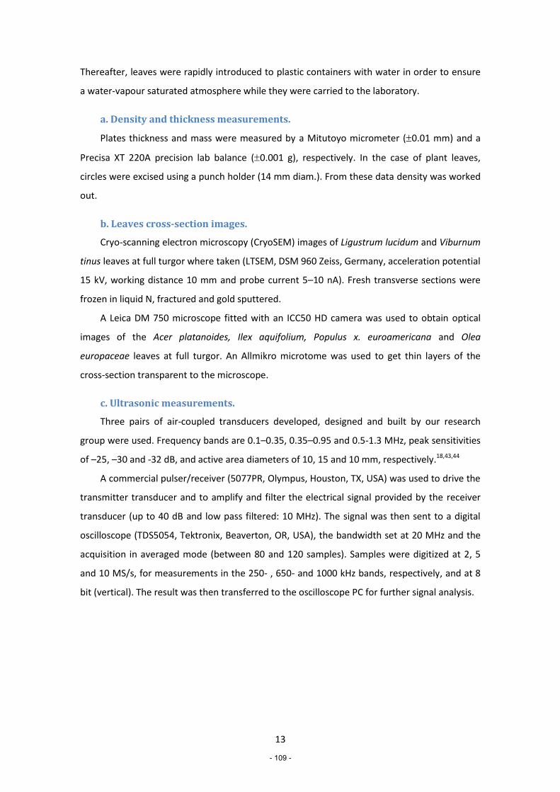
13

Thereafter, leaves were rapidly introduced to plastic containers with water in order to ensure

a water-vapour saturated atmosphere while they were carried to the laboratory.

a. Density and thickness measurements.

Plates thickness and mass were measured by a Mitutoyo micrometer (0.01 mm) and a

Precisa XT 220A precision lab balance (0.001 g), respectively. In the case of plant leaves,

circles were excised using a punch holder (14 mm diam.). From these data density was worked

out.

b. Leaves cross-section images.

Cryo-scanning electron microscopy (CryoSEM) images of Ligustrum lucidum and Viburnum

tinus leaves at full turgor where taken (LTSEM, DSM 960 Zeiss, Germany, acceleration potential

15 kV, working distance 10 mm and probe current 5–10 nA). Fresh transverse sections were

frozen in liquid N, fractured and gold sputtered.

A Leica DM 750 microscope fitted with an ICC50 HD camera was used to obtain optical

images of the Acer platanoides, Ilex aquifolium, Populus x. euroamericana and Olea

europaceae leaves at full turgor. An Allmikro microtome was used to get thin layers of the

cross-section transparent to the microscope.

c. Ultrasonic measurements.

Three pairs of air-coupled transducers developed, designed and built by our research

group were used. Frequency bands are 0.1–0.35, 0.35–0.95 and 0.5-1.3 MHz, peak sensitivities

of –25, –30 and -32 dB, and active area diameters of 10, 15 and 10 mm, respectively.18,43,44

A commercial pulser/receiver (5077PR, Olympus, Houston, TX, USA) was used to drive the

transmitter transducer and to amplify and filter the electrical signal provided by the receiver

transducer (up to 40 dB and low pass filtered: 10 MHz). The signal was then sent to a digital

oscilloscope (TDS5054, Tektronix, Beaverton, OR, USA), the bandwidth set at 20 MHz and the

acquisition in averaged mode (between 80 and 120 samples). Samples were digitized at 2, 5

and 10 MS/s, for measurements in the 250- , 650- and 1000 kHz bands, respectively, and at 8

bit (vertical). The result was then transferred to the oscilloscope PC for further signal analysis.

- 109 -

14

6. Results

a. Microscopic images of the leaves cross-section.

Figure 2 shows typical CryoSEM cross-section images of some of the leaves studied. Layers

from left to right are: adaxial epidermis, palisade parenchyma, spongy mesophyl and abaxial

epidermis.

Figure 2.- CryoSEM cross section micrographs of L. lucidum I and II and V. tinus.

Figure 3 shows representative cross-section optical images of Populus nigra, Acer

platanoides, Ilex aquifolium and Olea europaceae leaves. In this case, layers from top to

bottom are: adaxial epidermis, palisade parenchyma, spongy mesophyl and abaxial epidermis.

The bilayer structure of the leaf can be clearly seen in all cases, in some cases, disrupted by

thick epidermis layers or by the vascular system.

Figure. 3 – Optical microscope image of cross-sections of P. nigra, A. platanoides, I. aquifolium and

O. europaea leaves.

- 110 -

15

b. Results obtained using computer generated target spectra (TS).

TS were computer generated using the data in Table II for all 11 different bilayers (A-G).

Two different frequency ranges were used: i) 0.1-1.6 MHz with 𝐿𝑒𝑛{𝑓𝑖} = 180 points and ii)

0.1-3.2 with 𝐿𝑒𝑛{𝑓𝑖} = 360 points. The only missing data in Table II is n for cellulose 1 and 2,

which was not obtained experimentally, for these cases n was set equal to 0.95. To facilitate

the comparison of the extracted α, its value has always been recalculated at the same

frequency as they appear in Table I. Obtained values of 𝑚𝑒𝑎𝑛{𝑥𝑖𝑒} and 𝑠𝑡𝑑{𝑥𝑖

𝑒} appear in Table

III. Mean value of 휀 (Eq. 15) was very low (between 9 x 10-4 and 1.0 x 10-2) and the averaged

time of execution was typically about 2.5 minutes using a PC fitted with an i5, 3.2 GHz, Intel®

Core™ processor.

Table III. Extracted layer parameters [ 𝑚𝑒𝑎𝑛 𝑣𝑎𝑙𝑢𝑒𝑠𝑡𝑎𝑛𝑑𝑎𝑟𝑑 𝑑𝑒𝑣.

] from the computer generated TS in

synthetic bilayers. Hi-Z layer: first two rows, Lo-Z layer (last two rows).

Bilayer Thickness (µm)

Velocity (m/s)

Density (kg/m

3)

α @ f0 (Np/m)

n

A

2074.27 1679.29 1465.30 39.73 0.66

3.63 9.68 17.42 0.62 0.04

901.37 855.65 1349.15 33.96 0.58

4.77 7.61 43.48 2.00 0.11

A2

1037.04 1666.64 1433.73 68.15 0.59

15.55 29.08 26.30 7.16 0.08

920.75 881.36 1358.66 26.65 0.58

19.00 19.11 26.05 2.66 0.00

B

3199.90 1879.55 1017.21 40.65 0.84

9.99 8.97 9.65 2.35 0.06

990.11 948.11 966.18 39.71 0.57

0.00 1.33 18.36 3.87 0.06

C

4351.82 2716.25 1639.92 18.25 0.74

13.28 10.03 10.78 1.95 0.11

1093.44 1047.86 880.24 28.76 0.63

14.71 14.58 11.51 2.32 0.08

D

1267.96 1520.47 631.90 107.00 0.57

3.75 7.40 8.64 16.05 0.13

93.54 120.30 539.52 2166.92 1.82

2.08 3.24 164.78 184.57 0.05

E

1014.25 1473.44 666.17 131.05 0.70

3.18 4.97 12.86 5.74 0.09

95.67 123.18 383.99 1986.52 1.86

2.88 3.31 185.90 75.88 0.01

E2

612.82 1467.82 670.80 201.45 0.50

1.40 1.37 8.40 15.47 0.05

97.12 124.58 302.25 1912.79 1.88

0.00 0.40 11.27 121.60 0.04

F

226.10 697.54 1082.46 2269.89 0.96

3.28 9.44 15.97 593.90 0.17

94.33 120.57 408.07 2116.59 1.74

- 111 -

16

2.80 3.65 26.87 93.04 0.02

F2

301.30 693.13 1112.94 1559.69 1.02

0.00 3.50 7.14 158.45 0.08

95.43 121.71 453.50 2029.77 1.81

0.75 0.85 12.72 2.71 0.01

G

232.09 717.51 1070.06 2043.44 1.24

1.18 1.61 0.78 295.50 0.12

124.22 205.41 436.93 928.42 0.92

0.52 0.89 6.62 24.90 0.01

G2

308.97 713.07 1081.42 1588.76 0.96

4.97 16.45 32.60 49.15 0.02

126.68 208.73 461.84 796.86 0.84

5.03 9.41 66.33 24.00 0.14

c. Results obtained using measured target spectra (TS).

c.1. Polymeric bilayers.

Figures 4 and 5 show some of the measured TS. In addition, calculated TC using the one

layer model and 𝑆06𝑑𝐵: 𝑇𝐶1)(𝑆0

6𝑑𝐵)𝑐𝑎𝑙𝑐

(dashed grey line) and calculated TC using the two-

layer model and full spectrum: 𝑇𝐶(𝑆0)𝑐𝑎𝑙𝑐 (solid red line) are also shown. Vertical (blue) lines

indicate the expected frequency location of the series of thickness resonances of each layer,

for negligible coupling between resonances, calculated using the 𝑣/𝑡 data from Table II and

Eqs 13: 𝐿1(𝜆 4⁄ )|𝑛 (dashed line), and 𝐿2(𝜆 2⁄ )|𝑛 (solid line). Extracted values of 𝑚𝑒𝑎𝑛{𝑥𝑖𝑒} and

𝑠𝑡𝑑{𝑥𝑖𝑒} appear in Table IV. As expected, value of 휀 (𝑇𝐶(𝑆0)𝑐𝑎𝑙𝑐 , 𝑇𝐶) is larger than in the

previous case and varies from 0.03-0.05 (A, B and G2) up to 0.23 and 0.43 for D and C,

respectively. Averaged time of execution in an i5, 3.2 GHz, Intel® Core™ processor PC was

about 8 minutes.

- 112 -

17

Figure 4. –TC spectra vs. frequency. Circles: Measured TS for A-C bilayers. Dashed grey line:

𝑇𝐶1)(𝑆06𝑑𝐵)

𝑐𝑎𝑙𝑐 . Solid red line: 𝑇𝐶(𝑆0)𝑐𝑎𝑙𝑐.

-90

-80

-70

-60

-50

-40

A

0

20

40

60

80

-90

-80

-70

-60

-50

-40B

Ma

gn

itu

de

(d

B)

(

(

(

(

0

20

40

60

80

100

120

Ph

ase

(ra

d)

0.2 0.4 0.6 0.8 1.0

-100

-90

-80

-70

-60

-50

-40C

Frequency (MHz)

(

((

(

(

( (

(

0

30

60

90

120

150

180

- 113 -

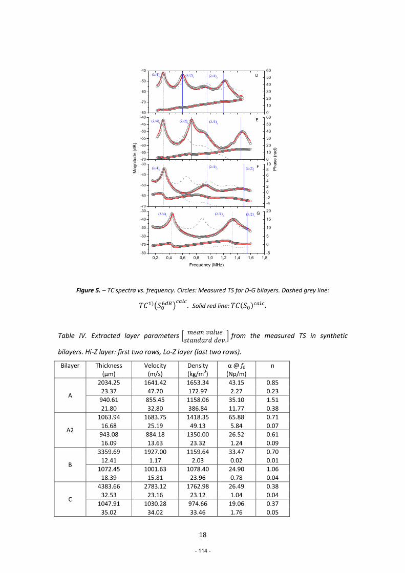
18

-80

-70

-60

-50

-40

D

0

10

20

30

40

50

60

-70

-65

-60

-55

-50

-45

-40

G

E

Ma

gn

itu

de

(d

B)

0

10

20

30

40

50

60

Ph

ase

(ra

d)

-70

-60

-50

-40

-30F

-4

-2

0

2

4

6

8

10

0,2 0,4 0,6 0,8 1,0 1,2 1,4 1,6 1,8

-80

-70

-60

-50

-40

-30

Frequency (MHz)

-5

0

5

10

15

20

Figure 5. – TC spectra vs. frequency. Circles: Measured TS for D-G bilayers. Dashed grey line:

𝑇𝐶1)(𝑆06𝑑𝐵)

𝑐𝑎𝑙𝑐. Solid red line: 𝑇𝐶(𝑆0)𝑐𝑎𝑙𝑐.

Table IV. Extracted layer parameters [ 𝑚𝑒𝑎𝑛 𝑣𝑎𝑙𝑢𝑒𝑠𝑡𝑎𝑛𝑑𝑎𝑟𝑑 𝑑𝑒𝑣.

] from the measured TS in synthetic

bilayers. Hi-Z layer: first two rows, Lo-Z layer (last two rows).

Bilayer Thickness (µm)

Velocity (m/s)

Density (kg/m

3)

α @ f0 (Np/m)

n

A

2034.25 1641.42 1653.34 43.15 0.85

23.37 47.70 172.97 2.27 0.23

940.61 855.45 1158.06 35.10 1.51

21.80 32.80 386.84 11.77 0.38

A2

1063.94 1683.75 1418.35 65.88 0.71

16.68 25.19 49.13 5.84 0.07

943.08 884.18 1350.00 26.52 0.61

16.09 13.63 23.32 1.24 0.09

B

3359.69 1927.00 1159.64 33.47 0.70

12.41 1.17 2.03 0.02 0.01

1072.45 1001.63 1078.40 24.90 1.06

18.39 15.81 23.96 0.78 0.04

C

4383.66 2783.12 1762.98 26.49 0.38

32.53 23.16 23.12 1.04 0.04

1047.91 1030.28 974.66 19.06 0.37

35.02 34.02 33.46 1.76 0.05

- 114 -

19

D

1177.65 1431.04 660.91 100.28 0.36

2.32 3.72 8.12 4.19 0.07

90.74 114.82 439.67 2915.93 1.64

2.19 2.89 122.84 252.15 0.04

E

957.78 1410.78 686.62 96.20 1.51

3.25 0.40 13.79 9.94 0.13

94.39 117.14 377.21 2435.09 1.33

0.00 0.51 124.63 45.38 0.02

E2

651.90 1425.99 677.76 181.95 0.55

1.93 5.28 6.47 24.16 0.11

104.31 134.02 357.49 1858.61 1.89

1.06 1.45 110.87 135.24 0.03

F

212.59 614.81 945.59 2310.14 0.47

0.00 2.41 2.32 210.95 0.05

86.52 108.62 382.22 2465.19 1.59

0.04 0.23 17.01 46.23 0.01

F2

336.65 704.13 1093.17 1388.82 1.15

4.57 7.53 21.33 325.71 0.21

105.05 134.07 414.50 1859.08 1.90

3.19 4.16 51.72 195.65 0.08

G

223.21 718.08 1128.73 2071.98 1.54

0.00 5.40 24.75 430.05 0.19

118.78 211.21 342.04 546.16 0.29

0.00 0.03 7.50 68.00 0.19

G2

345.57 706.33 1062.82 1542.02 1.22

1.46 10.40 54.59 72.08 0.03

140.20 230.60 530.49 547.44 0.59

1.46 4.10 126.89 44.68 0.26

c.2 Plant leaves.

Figures 6-8 show measured TS for the plant leaves. As before, calculated TC spectra using

the parameters extracted by the one layer model 𝑆06𝑑𝐵and TS6dB: 𝑇𝐶1)(𝑆0

6𝑑𝐵)𝑐𝑎𝑙𝑐

(dashed

grey line) and calculated TC using the two-layer model and full spectrum: 𝑇𝐶(𝑆0)𝑐𝑎𝑙𝑐 (solid red

line) are also shown. Finally, vertical (blue) lines indicate the expected frequency location of

the series of thickness resonances of each layer, for negligible coupling between resonances,

calculated using the 𝑣/𝑡 data extracted from the fitting of TS with the two layers model (Table

V) and Eqs 13: 𝐿1(𝜆 4⁄ )|𝑛 (dashed line), and 𝐿2(𝜆 2⁄ )|𝑛 (solid line), with 𝑛 = 1, 2, 3, …

Obtained 𝑚𝑒𝑎𝑛{𝑥𝑖𝑒} and 𝑠𝑡𝑑{𝑥𝑖

𝑒} appear in Table V.

- 115 -

20

Figure 6. Magnitude and phase spectra of TC vs. frequency for L. lucidum I and II leaves. Circles:

Measured TS. Dashed grey line: 𝑇𝐶1)(𝑆06𝑑𝐵)

𝑐𝑎𝑙𝑐. Solid red line: 𝑇𝐶(𝑆0)𝑐𝑎𝑙𝑐.

Figure 7. Magnitude and phase spectra of TC vs. frequency for for P. nigra and A. platanoides leaves.

Circles: Measured TS. Dashed grey line: 𝑇𝐶1)(𝑆06𝑑𝐵)

𝑐𝑎𝑙𝑐. Solid red line: 𝑇𝐶(𝑆0)𝑐𝑎𝑙𝑐.

-80

-70

-60

-50

-40 (

(

( Ligustrum lucidum I

-2

0

2

0.25 0.50 0.75 1.00 1.25 1.50

-90

-80

-70

-60

-50

-40(

(

(

Ma

gn

itu

de

(d

B)

Frequency (MHz)

Ligustrum lucidum II

-4

-2

0

2

Ph

ase

(ra

d)

-70

-60

-50

-40 (

(

( Populus nigra

-1.6

-0.8

0.0

0.8

1.6

2.4

0.25 0.50 0.75 1.00 1.25 1.50 1.75 2.00 2.25 2.50

-70

-60

-50

-40(

(

Ma

gn

itu

de

(d

B)

Frequency (MHz)

Acer platanoides

-1.6

-0.8

0.0

0.8

1.6 Ph

ase

(ra

d)

- 116 -

21

Figure 8. Magnitude and phase spectra of TC vs. frequency for for V. tinus, V. vinifera, O. europaea and I.

aquifolium leaves. Circles: Measured TS. Dashed grey line: 𝑇𝐶1)(𝑆06𝑑𝐵)

𝑐𝑎𝑙𝑐. Solid red line: 𝑇𝐶(𝑆0)𝑐𝑎𝑙𝑐.

Table V. Extracted layer parameters [ 𝑚𝑒𝑎𝑛 𝑣𝑎𝑙𝑢𝑒𝑠𝑡𝑎𝑛𝑑𝑎𝑟𝑑 𝑑𝑒𝑣.

] from the measured TS in plant leaves of

different species. Hi-Z layer: first two rows, Lo-Z layer (last two rows).

Species Thickness (µm)

Velocity (m/s)

Density (kg/m

3)

α @ f0 (Np/m)

n f0 (kHz)

Ilex aquifolium

402.07 987.35 972.90 2227.98 0.25

0.22 15.26 32.52 30.23 133.58 0.02

358.55 286.08 525.17 743.64 1.39

14.26 11.56 32.52 17.67 0.00

Arabidopsis thaliana

145.52 90.15 780.79 6623.97 1.19

0.14 3.82 2.66 52.06 536.84 0.07

123.43 70.26 383.08 7045.46 2.39

4.66 2.24 51.50 1129.18 0.14

Ligustrum lucidum I

413.34 510.78 1270.86 735.82 2.25

0.30 2.42 2.69 6.53 38.72 0.07

130.74 158.29 980.85 2245.13 1.32

1.35 1.81 59.06 18.07 0.03

Ligustrum lucidum II

237.57 558.76 1059.46 4671.80 0.50

0.28 1.95 14.68 17.95 459.45 0.06

106.74 109.21 669.06 2729.70 1.58

4.74 4.72 63.15 202.47 0.02

Viburnum tinus

149.62 588.91 1079.34 9421.53 1.42 0.46

2.94 7.56 18.98 817.00 0.08

-70

-60

-50

-40 (

Viburnum tinus(

-1.6

-0.8

0.0

0.8

1.6

-70

-60

-50

-40(

(

(

Ma

gn

itu

de

(d

B)

Vitis vinifera

-2.4

-1.6

-0.8

0.0

0.8

1.6

-80

-70

-60

-50

-40

(

(

(

( Olea europaea

-2.4

-1.6

-0.8

0.0

0.8

1.6

(

Ph

ase

(ra

d)

0.25 0.50 0.75 1.00 1.25 1.50 1.75

-100

-90

-80

-70

-60

-50

-40 (

(

(

Frequency (MHz)

Ilex aquifolium

-2

0

2

4

6

8

10

12

14

- 117 -

22

130.51 208.96 811.58 2168.86 1.24

1.97 2.84 13.95 44.48 0.03

Olea europaea

174.04 490.02 821.57 293.28 0.16

0.27 0.10 13.28 10.13 104.91 0.06

225.62 222.21 259.06 2455.36 0.99

2.33 1.26 11.40 49.99 0.03

Vitis vinifera

131.91 388.36 1090.50 5867.30 1.45

0.57 3.53 14.15 77.05 1212.59 0.28

88.67 193.39 614.61 6102.68 2.43

3.00 6.66 128.10 487.05 0.13

Populus nigra

135.02 389.45 1222.06 1543.79 3.68

0.70 1.75 3.23 46.59 298.55 0.21

73.85 208.60 766.71 7881.11 1.87

0.96 3.02 63.01 353.72 0.04

Acer platanoides

106.20 543.71 890.13 5871.28 0.58

0.65 1.35 9.66 17.68 1185.28 0.01

81.02 178.73 887.57 4550.66 2.08

0.87 1.89 25.09 331.27 0.02

In order to have an estimation of the intrinsic variability of leaf parameters, 15

different leaves of V. tinus were measured during the period November 2014 - April 2015.

Obtained values of 𝑚𝑒𝑎𝑛{𝑥𝑖𝑒} and 𝑠𝑡𝑑{𝑥𝑖

𝑒} appear in Table VI.

Table VI. Extracted layer parameters [ 𝑚𝑒𝑎𝑛 𝑣𝑎𝑙𝑢𝑒𝑠𝑡𝑎𝑛𝑑𝑎𝑟𝑑 𝑑𝑒𝑣.

] from the measured TS in 15 different

leaves of Viburnum tinus. Hi-Z layer: first two rows, Lo-Z layer (last two rows).

Species Thickness (µm)

Velocity (m/s)

Density (kg/m

3)

α @ f0 (Np/m)

n

Viburnum tinus

162.08 602.32 911.31 6841.74 1.30 19.88 148.70 101.36 3073.23 0.50

133.88 214.57 835.50 2550.16 1.36 18.29 22.77 108.75 319.92 0.27

As plant leaves are expected to be orthotropic, let us denote the thickness direction

with the number 3, then, the obtained elastic constant from thickness resonances and in the

transmission coefficient at normal incidence, in matrix format, is c33, which is obtained by:

𝑐33 = 𝑣2𝜌 (16)

In addition, if Poisson’s ratio () is known it is then possible to work out the Young’s

modulus (E). Results for 𝑐33 and E (assuming = 0.35),25,45 are summarized in Table VII.

Table VII. Elastic constant (c33) and Young modulus (E33) in the direction normal to the leaf plane

(mean value and standard deviation).

- 118 -

23

Layer c33 (MPa)

c33

(MPa)

E33 (MPa)

E33

(MPa)

I. aquifolium HiZ 948.45 45.98 640.13 31.03

LoZ 42.98 3.07 29.01 2.07

A.thaliana HiZ 6.35 0.40 4.28 0.27

LoZ 1.89 0.19 1.28 0.13

L. lucidum I HiZ 331.56 2.60 223.78 1.75

LoZ 24.58 1.02 16.59 0.69

L. lucidum II HiZ 330.78 11.49 223.25 7.76

LoZ 7.98 0.72 5.39 0.49

V.tinus HiZ 374.34 8.10 252.65 5.46

LoZ 35.44 0.79 23.92 0.53

O. europaea HiZ 197.28 6.56 133.15 4.43

LoZ 12.79 0.35 8.63 0.24

P.nigra HiZ 164.47 11.81 111.01 7.97

LoZ 22.99 3.19 15.51 2.15

A. platanoides HiZ 185.35 5.07 125.10 3.42

LoZ 33.36 1.85 22.52 1.25

7. Discussion.

The main objective of this work is to determine the possibility to establish a procedure

to extract the properties of the component layers of bilayer composites (layer decomposition)

with an emphasis on plant leaves for species where a bilayer acoustic model can be a realistic

or physiologically meaningful representation of the leaf structure. With the purpose to check

the accuracy of the layer decomposition procedure proposed it was first tested on eleven

synthetic bilayers made of well known layers (see Table II). The criterion selected is that layer

properties are properly extracted when:

𝑚𝑒𝑎𝑛{𝑥𝑖𝑒} − 𝑠𝑡𝑑{𝑥𝑖

𝑒} < {𝑥𝑖∗} < 𝑚𝑒𝑎𝑛{𝑥𝑖

𝑒} + 𝑠𝑡𝑑{𝑥𝑖𝑒} (18.1)

or

𝑚𝑖𝑛 (|𝑚𝑒𝑎𝑛{𝑥𝑖

𝑒}±𝑠𝑡𝑑{𝑥𝑖𝑒}−{𝑥𝑖

∗}|

{𝑥𝑖∗}

) < 0.05 (18.2)

In addition, we consider 𝑠𝑡𝑑{𝑥𝑖𝑒} > 10% as an indicator of the potential presence of

multiple solutions.

In a first step, TS for the synthetic bilayers were computer generated considering ideal

layers: layers completely flat, with uniform thickness, a perfect bounding between them,

normal incidence and a frequency range were four orders of the thickness resonances were

observed. In all cases the fitting of TC(S0)calc into TS is very good (ε 9 x 10-4 - 1 x 10-2). The

accuracy of extracted parameters can be evaluated by comparing 𝑚𝑒𝑎𝑛{𝑥𝑖𝑒} (Table III) with

{𝑥𝑖∗} (Table II) using criterion in Eqs. 18. The result of this comparison is summarized in Table

- 119 -

24

VIII. It is of interest the large value of 𝑠𝑡𝑑{𝜌𝐿𝑜𝑍𝑒 } in bilayers D and E which pointed out to the

appearance of several solutions. For example, two solutions are obtained for D with (𝜌𝐿𝑜𝑍𝑒 ,

𝜌𝐻𝑖𝑍𝑒 ) equal to (628, 620) kg/m3 and (649, 325) kg/m3, both with 0.014, while three

solutions are obtained for E, where (𝜌𝐿𝑜𝑍𝑒 , 𝜌𝐻𝑖𝑍

𝑒 ) take the values: (679, 291), (658, 352) and

(654,597) kg/m3, respectively, all with 0.01. To rule out some of these solutions, tighter

restrictions (than those in Table I) should be imposed for these bilayers.

Table VIII Comparison of 𝑚𝑒𝑎𝑛{𝑥𝑖𝑒} and {𝑥𝑖

∗} obtained using computer generated TS (CG)

and measured (Exp) TS following the criteria in Eqs. 18. Asterisk denotes cases where

𝑠𝑡𝑑{𝑥𝑖𝑒} > 10%.

bilayer layer t v ρ α n

CG Exp CG Exp CG Exp CG Exp CG Exp

A HiZ * LoZ *

A2 HiZ LoZ

B HiZ

LoZ

C HiZ

LoZ

D HiZ LoZ * *

E HiZ

LoZ * *

E2 HiZ LoZ *

F HiZ n.a

LoZ n.a

F2 HiZ n.a

LoZ * n.a

G HiZ n.a

LoZ n.a

G2 HiZ n.a

LoZ * n.a

Then TS for these 11 bilayers were measured. In this case, TS deviated from the ideal case

by some potential sources of error: the lack of perfectly flat surfaces, the non uniform

thickness of the layers, the presence of a layer of glue (or gel), the limited beam aperture and

diffraction (incidence is not perfectly normal), the limited SNR and the limited frequency

domain. As a result of all these features, is expected to be larger than in the previous case

and the accuracy of {𝑥𝑖𝑒} compared with {𝑥𝑖

∗} lower. Results are summarized in Table VIII,

where the agreement between expected and extracted thicknesses and velocities is, in

general, very good. As before, multiple solutions appear for bilayers D and E, but also for A, E2

and G2. For example, in bilayer A there are two solutions: S1 with 1 = 1510 50 kg/m3, 2 =

- 120 -

25

1470 90 kg/m3, and S2 with 1 = 1780 95 kg/m3, 2 = 860 150 kg/m3, where the first one is

very close to the expected values. Therefore, in this case, it would be necessary to further

restrict the constrains in order to be able to exclude one of these two solutions.

The largest errors are obtained in {𝑛𝑖𝑒}, this is because a good estimation of these

parameters requires the observation of, at least, two orders of the thickness resonances for

each of the layers and this is not true for bilayers F and G, and for bilayers D and E, one of

these resonances appears very damped or hidden within another one. In consequence, as {𝑛𝑖𝑒}

are used to recalculate the measured attenuation at the same frequency as they were

measured for each plate (Table II), then, {𝛼𝑖𝑒} are affected by the error in {𝑛𝑖

𝑒}. However,

extracted {𝛼𝑖𝑒} at the resonant frequencies in the bilayer composite are expected to be much

more accurate.

Results show that the soft or rigid nature of the materials the bilayer is made of is

determinant for the degree of coupling between resonances. Location of the resonances of

bilayers (Fig. 4) significantly deviated away from the expected /4 and /2 series. However, for

soft bilayers (Fig. 5) this deviation is much smaller. As this feature may have significant

implications in the determination of the initial guess in future applications. This behavior is

further investigated by calculating the location of the thickness resonances for two particular

cases: a soft and a rigid bilayer (see Table IX) where the ratio v/t for the high impedance layer

(𝑣 𝑡⁄ )𝐻𝑖𝑍 is changed from (𝑣 𝑡⁄ )𝐻𝑖𝑍 = (𝑣 𝑡⁄ )0 to (𝑣 𝑡⁄ )𝐻𝑖𝑍 = 10 × (𝑣 𝑡⁄ )0 . The value of

(𝑣 𝑡⁄ )𝐻𝑖𝑍 in Table IX corresponds to (𝑣 𝑡⁄ )0.

Table IX. Properties of soft and rigid bilayer composites used for calculations in Figs. 9 and 10.

Soft bilayer Rigid bilayer

LoZ HiZ LoZ HiZ

Z (MRayl) 0.089 0.762 1.21 2.41

v/t (MHz) 1.65 1.28 0.96 0.80

ρsup (kg/m2) 0.054 0.593 1.26 2.99

n 0.75 0.75 1.2 0.7

αt 0.093 0.320 0.023 0.086

Figures 9 and 10 show the location of the thickness resonances (red dots) versus

(𝑣 𝑡⁄ )𝐻𝑖𝑍. Horizontal solid (blue) lines represent the location of the /4 series of resonances

{𝑓𝐿𝑜𝑍𝑛 }, while solid (black) curves represent the location of the /2 series of resonances {𝑓𝐻𝑖𝑍

𝑛 }.

Actual magnitude spectra of the transmission coefficient for three different (𝑣 𝑡⁄ )𝐻𝑖𝑍 values

are shown in the three windows on the bottom of the figures. These frequencies are indicated

- 121 -

26

in the main figure with vertical lines. For soft bilayers the frequencies of the thickness

resonances are located very close to either {𝑓𝐿𝑜𝑍𝑛 } or {𝑓𝐻𝑖𝑍

𝑛 } (only some deviation at the

crossing points). On the contrary, for rigid bilayers there is a significant deviation over the

whole spectrum. In addition, it is observed that the first /4 resonance shifts towards higher

frequencies when (𝑣 𝑡⁄ )𝐻𝑖𝑍 becomes very large. Actually, theory predicts that when

(𝑣 𝑡⁄ )𝐻𝑖𝑍 → ∞ the {𝑓𝐿𝑜𝑍𝑛 } (which is a /4-series) becomes a /2-series. The location of this

transition from /4 to /2 resonance for the LoZ layer also depend on the impedances of the

both layers: the closer the impedances are the sooner will the transition take place.

Figure. 9. Variation in the location of the thickness resonances of the soft bilayer in Table IX vs (𝑣 𝑡⁄ )𝐻𝑖𝑍

and comparison with the location of the individual resonances of each layer.

- 122 -

27

Figure. 10. Variation in the location of the thickness resonances of the rigid bilayer in Table IX vs

(𝑣 𝑡⁄ )𝐻𝑖𝑍 and comparison with the location of the individual resonances of each layer.

For plant leaves, and in spite of the fact that the leaf structure is not exactly a bilayer

composite, that layers are, by far, not flat, thicknesses are not uniform and vascular system

and epidermis are ignored, the fitting of the model into the measured TS is very good in all

cases, which suggests that the bilayer model is a good representation of the acoustic response

of the leaves. The lowest resonant frequency observed corresponds, in all cases, to the first

/4 thickness resonance of the LoZ layer. In all cases either one or none orders of the thickness

resonances of the HiZ layer are observed, therefore obtained value of n for this layer should be

disregarded. Finally, in some cases, even the first order thickness resonance of the PP layer lies

out of the experimental frequency range (A. platanoides, V. tinus and O. europaea), so the

accuracy of the extracted values is also expected to be low.

Thickness of the leaves measured directly on micrographs in Figs. 2 and 3 are in good

agreement with data in Table V. For A. thaliana, published data39 reveal SM and PP tissues

porosities about 55% and 25%, respectively,40 this implies density values for SM and PP layers

in the range (550-635) and (250-290) kg/m3, respectively, which are not far from the extracted

density values for the HiZ and LoZ layers (Table V): (781 ± 52) and (383 ± 51) kg/m3,

respectively, where the shift towards higher values can be due to variability between different

cultivars.

We can further analyze the accuracy of the extracted parameters by checking the

consistency between them, the measured TS and the main microstructure features observed

in Figs. 2 and 3. For example, the main differences between L. Lucidum I and II in Fig 2 are the

much larger PP layer in type I leaves and the larger porosity of the SM layer in type II leaves.

This is consistent with the observed much lower frequency of (𝜆 2⁄ )1 for L. Lucidum I, and the

slightly lower frequencies for (𝜆 4⁄ )1 and (𝜆 4⁄ )2 for L. Lucidum II. Extracted c33 is similar for

both HiZ layers in L. lucidum which is consistent with the similar cellular structure in both

cases, but c33 of the LoZ layer is much larger for type I than for type II leaves, which can be

explained by the larger porosity in the SM layer of the type II leaves and the more elongated

cells in the thickness direction for type I leaves. In addition, other features that can contribute

to this difference are a thicker and/or more lignified cell wall in type I leaves.

The lowest 𝜌𝐿𝑜𝑍 is obtained for O. europaea, which is consistent with images in Fig. 3,

where the largest porosity appears in the SM layer of this species. According to Fig. 3, the

species where the porosity of SM and PP layers is expected to be most similar is A. platanoides,

which agrees with data in Table V, where both densities are almost equal. Cellular features in

- 123 -

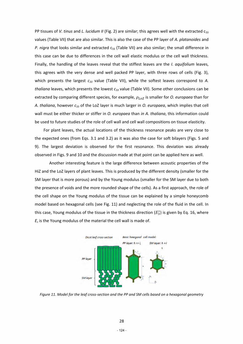
28

PP tissues of V. tinus and L. lucidum II (Fig. 2) are similar; this agrees well with the extracted c33

values (Table VII) that are also similar. This is also the case of the PP layer of A. platanoides and

P. nigra that looks similar and extracted c33 (Table VII) are also similar; the small difference in

this case can be due to differences in the cell wall elastic modulus or the cell wall thickness.

Finally, the handling of the leaves reveal that the stiffest leaves are the I. aquifolium leaves,

this agrees with the very dense and well packed PP layer, with three rows of cells (Fig. 3),

which presents the largest c33 value (Table VII), while the softest leaves correspond to A.

thaliana leaves, which presents the lowest c33 value (Table VII). Some other conclusions can be

extracted by comparing different species, for example, 𝜌𝐿𝑜𝑍 is smaller for O. europaea than for

A. thaliana, however c33 of the LoZ layer is much larger in O. europaea, which implies that cell

wall must be either thicker or stiffer in O. europaea than in A. thaliana, this information could

be used to future studies of the role of cell wall and cell wall compositions on tissue elasticity.

For plant leaves, the actual locations of the thickness resonance peaks are very close to

the expected ones (from Eqs. 3.1 and 3.2) as it was also the case for soft bilayers (Figs. 5 and

9). The largest deviation is observed for the first resonance. This deviation was already

observed in Figs. 9 and 10 and the discussion made at that point can be applied here as well.

Another interesting feature is the large difference between acoustic properties of the

HiZ and the LoZ layers of plant leaves. This is produced by the different density (smaller for the

SM layer that is more porous) and by the Young modulus (smaller for the SM layer due to both

the presence of voids and the more rounded shape of the cells). As a first approach, the role of

the cell shape on the Young modulus of the tissue can be explained by a simple honeycomb

model based on hexagonal cells (see Fig. 11) and neglecting the role of the fluid in the cell. In

this case, Young modulus of the tissue in the thickness direction (𝐸3∗) is given by Eq. 16, where

Es is the Young modulus of the material the cell wall is made of.

Figure 11. Model for the leaf cross-section and the PP and SM cells based on a hexagonal geometry

- 124 -

29

𝐸3∗ 𝐸𝑠⁄ = (

𝑡

𝑙)

3((ℎ 𝑙⁄ + 𝑠𝑖𝑛𝜃) 𝑐𝑜𝑠3𝜃⁄ ) (16)

However, the total Young modulus of the tissue in the thickness direction (𝐸3) will include

the deformability of the cell (Eq. 16), the role of the fluid in the cell and the cell volume

fraction ():

𝐸3 = 𝜙𝐸3∗ + 𝐸𝑓𝑙𝑢𝑖𝑑 (17)

The contribution of the fluid (𝐸𝑓𝑙𝑢𝑖𝑑) to the tissue elasticity takes place through the

compressibility of the fluid, therefore,46,47 if the cell is able to deform while keeping the cell

volume constant, then there will be no contribution of 𝐸𝑓𝑙𝑢𝑖𝑑 because there will be no strain in

the fluid. This situation is close to the case of SM cells proposed in Fig. 11 because 2D regular

hexagons can deformate along the 3 direction while keeping surface (volume) constant. Quite

on the contrary, as PP cells are elongated in the thickness direction, any cell length reduction

will produce a similar fluid compression, so 𝐸𝑓𝑙𝑢𝑖𝑑 will have a significant contribution for PP

cells. All these effects explain the large anisotropy in the Young modulus along the leaf

thickness direction. Let us consider one example, assume 𝐸𝑠 = 4 GPa, t/l = 0.075, l = 20 m,

ℎ𝑆𝑀 = 20 m, ℎ𝑃𝑃 = 200 m, 𝜙𝑃𝑃 = 0.9, 𝜙𝑃𝑃 = 0.6, and two values of 𝜃 = 20° and 60°,

then obtained values for 𝐸3∗𝑆𝑀 and 𝐸3

∗𝑃𝑃will be: 3.9 – 35.8 MPa (for SM) and 44.9 – 312.9 MPa

(for PP) for 𝜃 = 30° and 50°, respectively. These figures are similar to those obtained

experimentally (see table VII), where 𝐸3∗𝑆𝑀 varies from 1.28 - 5.39 MPa (A. thaliana and L.

lucidum II) up to 23.9 - 29.01 MPa (V. Tinus and I. aquifolium). While, 𝐸3∗𝑃𝑃 (see table VII) varies

from 4.28 – 111.0 MPa (A. thaliana and P. nigra), to 252.65 – 640.13 MPa (V. Tinus and I.

aquifolium), where these larger values can be due to the contribution of the fluid in the cells in

the case of the elongated cells of the PP tissue.

8. Conclusions.

A method for the layer decomposition of bilayer composites plates has been presented. It

takes the ultrasonic transmission coefficient spectra at normal incidence (TS) in the frequency

range were several thickness resonances are observed and returns thickness, density and

ultrasound velocity and attenuation for each of the constituent layers. Unlike the procedure to

extract layer properties of a one-layer plate,20,36 this procedure requires of some previous

knowledge of the composite (to set constrains) and some degree of supervision (to detect the

- 125 -

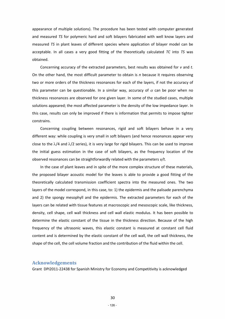
30

appearance of multiple solutions). The procedure has been tested with computer generated

and measured TS for polymeric hard and soft bilayers fabricated with well know layers and

measured TS in plant leaves of different species where application of bilayer model can be

acceptable. In all cases a very good fitting of the theoretically calculated TC into TS was

obtained.

Concerning accuracy of the extracted parameters, best results was obtained for v and t.

On the other hand, the most difficult parameter to obtain is n because it requires observing

two or more orders of the thickness resonances for each of the layers, if not the accuracy of

this parameter can be questionable. In a similar way, accuracy of can be poor when no

thickness resonances are observed for one given layer. In some of the studied cases, multiple

solutions appeared; the most affected parameter is the density of the low impedance layer. In

this case, results can only be improved if there is information that permits to impose tighter

constrains.

Concerning coupling between resonances, rigid and soft bilayers behave in a very

different way: while coupling is very small in soft bilayers (and hence resonances appear very

close to the /4 and /2 series), it is very large for rigid bilayers. This can be used to improve

the initial guess estimation in the case of soft bilayers, as the frequency location of the

observed resonances can be straightforwardly related with the parameters v/t.

In the case of plant leaves and in spite of the more complex structure of these materials,

the proposed bilayer acoustic model for the leaves is able to provide a good fitting of the

theoretically calculated transmission coefficient spectra into the measured ones. The two

layers of the model correspond, in this case, to: 1) the epidermis and the palisade parenchyma

and 2) the spongy mesophyll and the epidermis. The extracted parameters for each of the

layers can be related with tissue features at macroscopic and mesoscopic scale, like thickness,

density, cell shape, cell wall thickness and cell wall elastic modulus. It has been possible to

determine the elastic constant of the tissue in the thickness direction. Because of the high

frequency of the ultrasonic waves, this elastic constant is measured at constant cell fluid

content and is determined by the elastic constant of the cell wall, the cell wall thickness, the

shape of the cell, the cell volume fraction and the contribution of the fluid within the cell.

Acknowledgements Grant DPI2011-22438 for Spanish Ministry for Economy and Competitivity is acknowledged

- 126 -

31

References

1. P. Y. Chen, a. Y. M. Lin, Y. S. Lin, Y. Seki, a. G. Stokes, J. Peyras, E. a. Olevsky, M. a. Meyers and J.McKittrick, J. Mech. Behav. Biomed. Mater., 2008, 1, 208–226.

2. O. Shishkina, S. V. Lomov, I. Verpoest and L. Gorbatikh, Arch. Appl. Mech., 2014, 84, 789–805.3. S. Richter, J. Müssig and N. Gierlinger, Planta, 2011, 233, 763–72.4. S. Amada, Y. Ichikawa, T. Munekata, Y. Nagase and H. Shimizu, Compos. Part B Eng., 1997, 28,

13–20.5. V. I. Egorov, I. V. Schastlivtsev, E. V. Prut, A. O. Baranov and R. a. Turusov, J. Biomech., 2002, 35,

1417–1425.6. J. A. Motherway, P. Verschueren, G. Van der Perre, J. Vander Sloten and M. D. Gilchrist, J.

Biomech., 2009, 42, 2129–2135.7. M. A. Meyers, P.-Y. Chen, A. Y.-M. Lin and Y. Seki, Prog. Mater. Sci., 2008, 53, 1–206.8. J.-Z. Yang, X.-Z. Hu, R. Sultana, R. Edward Day, and P. Ichim, Biomedical Materials, 2015, 10(4),

045006.9. R. Fujioka,T. Aoyama, and T. Takakuwa, 2013. Osteoarthritis and Cartilage / OARS,

Osteoarthritis Research Society, 2013, 21(8), 1092–1098.10. L. J. Gibson, M. F. Ashby and B.A. Harley, Cellular materials in nature and medicine. Cambridge,

Cambridge, 1st edn., 2010.11. T. Faisal, A. Rey and D. Pasini, Polymers (Basel), 2013, 5, 730–750.12. K. J. Niklas. The Evolutionary Biology of Plants. Chicago: University of Chicago Press; 199713. Y. K. Murugesan, D. Pasini and A. D. Rey, Soft Matter, 2011, 7, 7078.14. A. Migliori and J. L. Sarrao, Resonant Ultrasound Spectroscopy, Wiley, New York, 1997.15. A. Migliori, J. Sarrao, W.M. Visscher, T.M. Bell, Ming Lei, Z. Fisk, and R.G. Leisure, Physica B,

1993, 183(1-2):1–24.16. B. J. Zadler, J. H. L. Le Rousseau, and J. A. Scales and M. L. Smith, Geophys. J. Int., 2004,

156:154–169.17. T. E. G. Alvarez-Arenas, F. R. Montero De Espinosa, M. Moner-Girona, E. Rodrıguez, A. Roig and

E. Molins, Appl. Phys. Lett., 2002, 81, 1198.18. T. E. G. Álvarez-Arenas, J. Memb. Sci., 2003, 213, 195–207.19. T. E. G. Alvarez-Arenas, H. Calas, J. E. Cuello, A. Fernandez, and M. Munoz, J. App. Phys. 2010,

108(7), 074110.20. T. E. G. Álvarez-Arenas, Ultrasonics, 2010, 50, 104–9.21. T. E. G. Alvarez-Arenas, D. Sancho-Knapik, J. J. Peguero-Pina and E. Gil-Pelegrin, Appl. Phys.

Lett., 2009, 95, 193702.22. D. Sancho-Knapik, T. E. G. Álvarez-Arenas, J. J. Peguero-Pina and E. Gil-Pelegrín, J. Exp. Bot.,

2010, 61, 1385–91.23. L. Taiz and E. Zeiger, Plant physiology. 3rd Ed. Sunderland: Sinauer Associates, 2002.24. Ghysels P., Samaey G., Van Liedekerke P., Tijskens E., Ramon H. and Roose D. Int. J. Multiscale

Com. Eng., 2010, 8(4), 379-396.25. M. D. Farinas, D. Sancho-Knapik, J. J. Peguero-Pina, E. Gil-Pelegrin and T. E. G. Alvarez-Arenas,

Appl. Phys. Lett., 2013, 102, 103702.26. M. D. Fariñas and T. E. G. Álvarez-Arenas, in 22nd International Congress on Sound and

Vibration, Florence, 2015, pp. 12–16.27. M. D. Fariñas, D. Sancho Knapik, J. J. Peguero Pina, E. Gil Pelegrin and T. E. G. Álvarez-Arenas,

Ultrasound Med. Biol., 2014, 1–12.28. L.M. Brekhovskikh, Waves in layered media. Academic Press, London. 1960.29. L. Flax, G. Gaunaurd, H. Überall, Theory of resonance scattering in Physical Acoustics, Vol. XV,

Academic Press, London. 1981.30. D.A. Hutchins, and W.M.D. Wright, J. Acoust. Soc. Am., 1994, 96(3), 1634–1642.31. W.T. Thomson, J. Appl. Phys., 1950, 21, 89-93..32. Y. Wang, Ph.D. thesis, Standford University, 1986.33. W. Cao and W. Qi. J. Appl. Phys., 1995, 78(7), 4627-4632.34. T.L. Szabo, J. Acoust. Soc. Am., 1995, 97, 14–24.35. H. Hoos and T. Stützle, Stochastic Local Search: Foundations and Applications, Morgan

Kaufmann Series in Artificial Inteligence, Elsevier, 2005.

- 127 -

32

36. D. Sancho-Knapik, H. Calás, J. J. Peguero-Pina, A. Ramos Fernández, E. Gil-Pelegrín and T. E. G.Álvarez-Arenas, IEEE Trans. Ultrason. Ferroelectr. Freq. Control Trans. Ultrason. Ferroelectr.Freq. Control, 2012, 59, 319–325.

37. C. Solnon. Ant colony optimization and constrain programming. John Wiley and Sons, Inc. 2010.

38. J.I.L. Morison, E. Galloue, T. Lawson, G. Cornic, R. Herbin, N.R. Baker, Plant Physiology, 2005,

139(1), 254–266.39. R. Pieruschka, J. Exp. Bot.., 2005, 56(413), 857–864.40. C. Dorca-Fornell et al., Plant Journal, 2013, 76(6), 914–929

41. I. Terashima. Photosynth Res, 1992, 31, 195–21242. I. Terashima, M. Ishibashi, K. Ono, K. Hikosaka, in 10

th International Photosynthesis Congress,

Dordrecht, 1996, pp. 537–54243. T.E.G. Álvarez-Arenas, IEEE Trans. Ultrason. Ferroelectr. Freq. Control, 2003, 50(6), 676-685.44. US-Biomat Air-Coupled ultrasound transducers: http://us-biomat.com/research/air-coupled-

ultrasound-transducers45. M. D. Fariñas and T. E. G. Álvarez-Arenas, J. Mech. Behav. Biomed. Mater., 2014, 39, 304–15.46. H. C. P. Karunasena, W. Senadeera, R. J. Brown and Y. T. Gu, Soft Matter, 2014, 10, 5249.

47. P. Van Liedekerke, P.Ghysels, E.Tijskens, G. Samaey, D. Roose and H. Ramon, Phys. Biol. 2010, 7026006.

- 128 -

CONCLUSIONES

CAPÍTULO 7.Conclusiones

- 129 -

M.D. FARIÑAS, 2016

- 130 -

“I like the scientific spirit—the holding off, the being sure but not too sure, the willingness to surrender ideas when the evidence is against them: this is ultimately fine—it always keeps the way beyond open—always gives life, thought, affection, the whole man, a chance to try over again after a mistake—after a wrong guess.”

Walt Whitman

Walt Whitman’s Camden Conversations. Walt Whitman. 1888.

CONCLUSIONES

Conclusiones Generales

La técnica de Espectroscopía Ultrasónica Resonante Sin Contacto (NC-RUS) permite obtener información diferenciada de los distintos tejidos que componen las hojas de plantas de un modo no invasivo, no destructivo e inmediato (Objetivo 1). Para ello, se excitan sus resonancias espesor usando transmisión directa e incidencia normal en el rango de frecuencias [0.1 – 1.6] MHz. Del análisis en la banda de frecuencia acotada a los alrededores de la primera resonancia (establecida entre 0.1 y 1 MHz en función de la especie, individuo, grado de desarrollo del tejido, etc.), se obtienen propiedades efectivas de la hoja como su espesor, densidad volumétrica, velocidad de propagación y atenuación, gracias a la resolución del problema inverso asumiendo la hoja como una lámina de material homogéneo. Del análisis en banda ancha considerando todo el espectro medido, se obtienen parámetros tales como impedancia acústica, densidad superficial, ratio velocidad-espesor y el producto de atenuación por espesor de cada una de las capas de tejido que conforman la hoja. Para tal fin, se asume que la hoja está formada por dos capas de tejido acústicamente diferentes. El algoritmo utilizado para la optimización del ajuste de los datos considerados con el modelo teórico es un Descenso de Gradiente Estocástico (SDG). Los valores de impedancia acústica calculados para las capas de tejido de alta impedancia consideradas (equivalentes a la epidermis superior y parénquima de empalizada) se establecen entre 0.1 y 1.1 MRayl. Sin embargo, en las capas de tejido de baja impedancia consideradas (equivalentes a epidermis inferior y mesófilo esponjoso) se establecen entre 0.05 y 0.4 MRayl. Estos valores son consistentes con las porosidades típicas observadas en el mesófilo esponjoso (entre el 30 y el 60 %) que dan lugar a gran variación en la densidad volumétrica.

Otras técnicas ultrasónicas que buscan la propagación de modos guiados en el plano de la hoja y ondas de cizalla, han sido utilizadas en la realización de esta tesis doctoral. Los datos han concluido que la excitación y detección de ondas de cizalla en hojas de plantas es posible y, del mismo modo, la obtención de los parámetros mecánicos transversales de estas (Objetivo 2). Los valores obtenidos de ratio de Poisson para las especies Vitis vinifera y Epipremnum aureum varían entre 0.33 y 0.34, lo cual concuerda con la estimación a partir de los datos disponibles en la bibliografía. Se constata que la propagación de las ondas de corte depende del estado de desarrollo y la especie en concreto bajo estudio y también, del contenido en agua de la hoja en cuestión. La propagación de ondas guiadas a lo largo de otros tipos de tejido que componen las hojas, como las fibras de esclerénquima, también se llevó a cabo con éxito en hojas de Phormium tenax, permitiendo así la evaluación de los diferentes parámetros elásticos que las conforman. Las células esclerenquimáticas tienen típicamente diámetros menores y paredes más gruesas, observándose velocidades de propagación ampliamente mayores que en los tejidos del mesófilo para la misma especie (700 – 900 m/s).

Por último, se realizaron experimentos in vivo sobre hojas que se mantuvieron unidas al resto de la planta. Se modificaron estímulos abióticos tales como: la luz (desde 2000 a 150 µmol/m2s) originando un aumento en la frecuencia de resonancia de entre el 8 y el

- 131 -

M.D. FARIÑAS, 2016 12% en menos de una hora; el agua (riego abundante tras un período corto de sequía) produciendo un incremento en la frecuencia fundamental de resonancias espesor entre un 5 y un 30% entre los siguientes 10 min y hasta 7 horas después; y también a consecuencia del ciclo día-noche, observándose cambios de entre el 4 y el 10% en la frecuencia de resonancia fundamental (Objetivo 3). Estos cambios se relacionaron con mecanismos de respuesta de las hojas que se traducen en alteraciones en la mecánica de estas.

Por tanto, la técnica NC-RUS ha demostrado ser la única capaz de tomar medidas de hojas de plantas de un modo no invasivo, no destructivo e inmediato, pudiendo recabar información in vivo de la respuesta de la hoja ante diferentes factores abióticos prolongada en el tiempo. Asimismo, permite calcular parámetros mecánicos transversales gracias a que puede excitar y detectar ondas de cizalla, así como propagar modos guiados. Por último, es también novedosa en tanto en cuanto permite la obtención de parámetros acústicos y mecánicos de diferentes capas de tejido que componen la hoja. En conclusión, la técnica NC-RUS ha demostrado ser capaz de obtener información no disponible hasta el momento sobre tejidos de hojas de plantas, de una manera ventajosa y única que incluye la no invasividad, la no destructividad, sin necesidad de contacto y de una manera rápida.

- 132 -

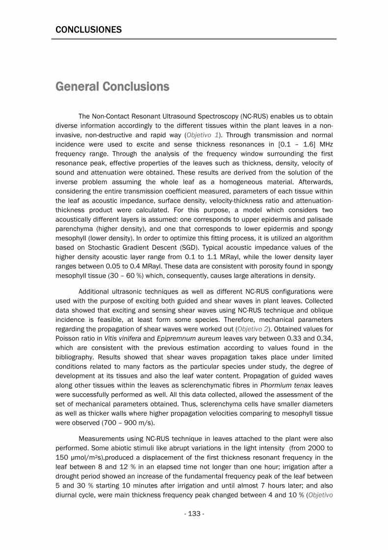
CONCLUSIONES

General Conclusions

The Non-Contact Resonant Ultrasound Spectroscopy (NC-RUS) enables us to obtain diverse information accordingly to the different tissues within the plant leaves in a non-invasive, non-destructive and rapid way (Objetivo 1). Through transmission and normal incidence were used to excite and sense thickness resonances in [0.1 – 1.6] MHz frequency range. Through the analysis of the frequency window surrounding the first resonance peak, effective properties of the leaves such as thickness, density, velocity of sound and attenuation were obtained. These results are derived from the solution of the inverse problem assuming the whole leaf as a homogeneous material. Afterwards, considering the entire transmission coefficient measured, parameters of each tissue within the leaf as acoustic impedance, surface density, velocity-thickness ratio and attenuation-thickness product were calculated. For this purpose, a model which considers two acoustically different layers is assumed: one corresponds to upper epidermis and palisade parenchyma (higher density), and one that corresponds to lower epidermis and spongy mesophyll (lower density). In order to optimize this fitting process, it is utilized an algorithm based on Stochastic Gradient Descent (SGD). Typical acoustic impedance values of the higher density acoustic layer range from 0.1 to 1.1 MRayl, while the lower density layer ranges between 0.05 to 0.4 MRayl. These data are consistent with porosity found in spongy mesophyll tissue (30 – 60 %) which, consequently, causes large alterations in density.

Additional ultrasonic techniques as well as different NC-RUS configurations were used with the purpose of exciting both guided and shear waves in plant leaves. Collected data showed that exciting and sensing shear waves using NC-RUS technique and oblique incidence is feasible, at least form some species. Therefore, mechanical parameters regarding the propagation of shear waves were worked out (Objetivo 2). Obtained values for Poisson ratio in Vitis vinifera and Epipremnum aureum leaves vary between 0.33 and 0.34, which are consistent with the previous estimation according to values found in the bibliography. Results showed that shear waves propagation takes place under limited conditions related to many factors as the particular species under study, the degree of development at its tissues and also the leaf water content. Propagation of guided waves along other tissues within the leaves as sclerenchymatic fibres in Phormium tenax leaves were successfully performed as well. All this data collected, allowed the assessment of the set of mechanical parameters obtained. Thus, sclerenchyma cells have smaller diameters as well as thicker walls where higher propagation velocities comparing to mesophyll tissue were observed (700 – 900 m/s).

Measurements using NC-RUS technique in leaves attached to the plant were also performed. Some abiotic stimuli like abrupt variations in the light intensity (from 2000 to 150 µmol/m2s),produced a displacement of the first thickness resonant frequency in the leaf between 8 and 12 % in an elapsed time not longer than one hour; irrigation after a drought period showed an increase of the fundamental frequency peak of the leaf between 5 and 30 % starting 10 minutes after irrigation and until almost 7 hours later; and also diurnal cycle, were main thickness frequency peak changed between 4 and 10 % (Objetivo

- 133 -

M.D. FARIÑAS, 2016 3). Some response mechanisms of leaves were proposed as the cause of these variations in the transmission coefficient spectra, which might be translated into mechanic alterations easily detected by the NC-RUS technique.

Henceforth, NC-RUS technique is capable of measuring plant leaves in a non-invasive, non-destructive and rapid way. This enables the collection of information in vivo about leaves’ response to changes in abiotic factors over time. Additionally, using NC-RUS technique, shear and guided waves can be excited and detected which permits obtaining mechanical transverse components of tissues within the leaves. Finally, NC-RUS is innovative since acoustic and mechanic parameters of different layers within the leaf can be extracted separately. In conclusion, the NC-RUS technique was proven to collect information not available so far about plant tissues in an advantageous and unique way which includes non-invasiveness, non-destructiveness, contactless and promptness.

- 134 -

PROSPECTIVA

CAPÍTULO 8. Prospectiva

- 135 -

M.D. FARIÑAS, 2016

- 136 -

“In the long run men hit only what they aim at. Therefore, though they should fall immediately, they had better aim at something high.”

Henry David Thoreau

Walden or Life in the Woods. Henry David Thoreau. 1854.

PROSPECTIVA

En algunas pruebas preliminares se ha podido comprobar cómo el efecto ya observado para el primer pico de resonancia de espesor en hojas durante la pérdida de contenido relativo de agua se sucede en banda ancha. Se espera que pueda obtenerse más información de cómo evolucionan los diferentes tejidos que conforman la hoja con la pérdida de agua.

Paralelamente, gracias a la amplia colección de datos de parámetros mecánicos recabados durante el desarrollo de la tesis doctoral, se ha modelizado la sección transversal de la hoja siguiendo un modelo geométrico tipo panal de abeja (honeycomb). En él, se distinguen dos tipos celulares que corresponden a los que forman los dos tejidos considerados en el modelo bicapa. Por tanto, un desarrollo más pormenorizado, sería interesante dados los buenos resultados previos obtenidos.

Durante los pasados dos años se han venido realizando experimentos en conjunto con científicos del Centro Nacional de Biotecnología (CNB) sobre distintas variedades genéticas de Arabidopsis thaliana, cuyo genoma se encuentra completamente secuenciado. En primera instancia, el fin de estos experimentos es comprobar si ciertos parámetros de los medidos con la técnica ultrasónica guardan alguna heredabilidad genética por encima de factores ambientales.

Prácticamente desde el comienzo de la aplicación de esta técnica ultrasónica en hojas de plantas, la Vitis vinífera ha sido una de las más recurrentes en los experimentos realizados, tanto por su espléndida respuesta ultrasónica como por su importancia industrial. Conocida la problemática en cuanto a la disminución en calidad de la uva debido a un riego excesivo, el control de este mediante un sistema de toma de decisiones en base a la monitorización activa de parámetros de ultrasonidos, parece una prometedora línea de investigación. Asimismo, hacerla extensiva a otros cultivos donde el ahorro de agua es crucial no sólo en lo relativo al aumento de producción, sino al aprovechamiento de agua como un fin en sí mismo. Las técnicas de Riego por Déficit Regulado (RDI) se están popularizando aunque se advierte de la necesidad del desarrollo de más métodos capaces de evaluar experimentalmente la respuesta de especies de cultivos específicos ante estas RDI (Chai et al. 2016). La técnica aquí presentada, parece competente en este aspecto.

Por otro lado, la producción de cultivos con el objetivo de maximizar la biomasa de estos, presenta una línea más centrada en el análisis del crecimiento del área foliar y su masa (Weraduwage et al. 2015). A grandes rasgos, el estudio de cómo diferentes especies o variedades genéticas de una misma planta varían su ratio de fotosíntesis o partición de carbono en favor de maximizar la biomasa, pasa por un crecimiento foliar en el que aspectos como el aumento de espesor de estas es crucial. Los métodos utilizados actualmente para medir estas variaciones, pasan por cortes micrográficos o uso del micrómetro. La Espectroscopía Ultrasónica Resonante Sin Contacto ha resultado ser muy efectiva también en cuantificar espesor.

Finalmente, se ha llegado a la conclusión de la importancia de la fenomenología a nivel foliar (especialmente al crecimiento y senescencia) en la regulación del flujo de agua y carbono en la superficie terrestre asociados a la respuesta climática (Wu et al. 2016). La

- 137 -

M.D. FARIÑAS, 2016 técnica que se ha presentado aquí, podría ayudar a entender mejor esta evolución y las bases fisiológicas para arrojar algo de luz sobre estos fenómenos fenológicos, ayudando hipotéticamente a predecir la respuesta a largo plazo de bosques y tomar decisiones en pro de la resiliencia contra el cambio climático global (Naudts et al. 2016; Reich et al. 2016).

- 138 -

REFERENCIAS

CAPÍTULO 9. Referencias

- 139 -

M.D. FARIÑAS, 2016

- 140 -

"Los que no quieren imitar nada, no producen nada."

Salvador Dalí

REFERENCIAS

AGIRRE OLABIDE, I., ELEJABARRIETA, M.J., BOU-ALI, M.M., FARIÑAS, M.D. y ÁLVAREZ-ARENAS, T.E.G., 2013. Modification of the ultrasonic properties of elastomers loaded with magnetic particles by applying magnetic fields during curing. 2013 IEEE International Ultrasonics Symposium (IUS) [en línea]. S.l.: IEEE, pp. 1101-1104. ISBN 978-1-4673-5686-2. DOI 10.1109/ULTSYM.2013.0282. Disponible en: http://ieeexplore.ieee.org/lpdocs/epic03/wrapper.htm?arnumber=6724889.

AGRAWAL, M., PRASAD, A., BELLARE, J.R. y SESHIA, A.A., 2016. Characterization of mechanical properties of materials using ultrasound broadband spectroscopy. Ultrasonics [en línea], vol. 64, pp. 186-195. ISSN 0041624X. DOI 10.1016/j.ultras.2015.09.001. Disponible en: http://linkinghub.elsevier.com/retrieve/pii/S0041624X15002231.

ALVAREZ-ARENAS, T.E.G., 2004. Acoustic impedance matching of piezoelectric transducers to the air. IEEE Transactions on Ultrasonics, Ferroelectrics and Frequency Control [en línea], vol. 51, no. 5, pp. 624-633. [Consulta: 3 marzo 2016]. ISSN 0885-3010. DOI 10.1109/TUFFC.2004.1320834. Disponible en: http://ieeexplore.ieee.org/lpdocs/epic03/wrapper.htm?arnumber=1320834.

ÁLVAREZ-ARENAS, T.E.G., 2003. Air-coupled ultrasonic spectroscopy for the study of membrane filters. Journal of Membrane Science [en línea], vol. 213, pp. 195-207. Disponible en: http://www.sciencedirect.com/science/article/pii/S0376738802005276.

ÁLVAREZ-ARENAS, T.E.G., 2010. Simultaneous determination of the ultrasound velocity and the thickness of solid plates from the analysis of thickness resonances using air-coupled ultrasound. Ultrasonics [en línea], vol. 50, no. 2, pp. 104-9. [Consulta: 25 febrero 2014]. ISSN 1874-9968. DOI 10.1016/j.ultras.2009.09.009. Disponible en: http://www.ncbi.nlm.nih.gov/pubmed/19819512.

ÁLVAREZ-ARENAS, T.E.G., MONTERO DE ESPINOSA, F.R., MONER-GIRONA, M., RODRIGUEZ, E., ROIG, A. y MOLINS, E., 2002. Viscoelasticity of silica aerogels at ultrasonic frequencies. Applied Physics Letters [en línea], vol. 81, no. 7, pp. 1198. ISSN 00036951. DOI 10.1063/1.1499225. Disponible en: http://link.aip.org/link/APPLAB/v81/i7/p1198/s1&Agg=doi.

ÁLVAREZ-ARENAS, T.E.G., SANCHO-KNAPIK, D., PEGUERO-PINA, J.J. y GIL-PELEGRIN, E., 2009. Noncontact and noninvasive study of plant leaves using air-coupled ultrasounds. Applied Physics Letters [en línea], vol. 95, no. 19, pp. 193702. ISSN 00036951. DOI 10.1063/1.3263138. Disponible en: http://link.aip.org/link/APPLAB/v95/i19/p193702/s1&Agg=doi.

ÁLVAREZ-ARENAS, T.E.G., SHROUT, T.R., ZHANG, S.J. y LEE, H.J., 2012. Air-coupled transducers based on 1-3 connectivity single crystal piezocomposites. 2012 IEEE International Ultrasonics Symposium [en línea]. S.l.: IEEE, pp. 2230-2233. ISBN 978-1-4673-4562-0. DOI 10.1109/ULTSYM.2012.0557. Disponible en: http://ieeexplore.ieee.org/lpdocs/epic03/wrapper.htm?arnumber=6562223.

ASTER, R.C., BORCHERS, B. y THURBER, C.H., 2013. Parameter Estimation and Inverse Problems. Oxford: Elsevier. ISBN 9788578110796.

BREKHOVSKIKH, L.M., 1980. Waves in Layered Media. 2nd. New York: Academic Press, inc. ISBN 0-12-130560-0.

- 141 -

M.D. FARIÑAS, 2016 BRODRIBB, T.J. y HOLBROOK, N.M., 2003. Stomatal closure during leaf dehydration,

correlation with other leaf physiological traits. Plant physiology, vol. 132, no. 4, pp. 2166-2173. ISSN 0032-0889. DOI 10.1104/pp.103.023879.

CAO, W. y QI, W., 1995. Plane wave propagation in finite 2-2 composites. Journal of Applied Physics, vol. 78, no. November 1994, pp. 4627-4632. ISSN 00218979. DOI 10.1063/1.360701.

CHAI, Q., GAN, Y., ZHAO, C., XU, H.L., WASKOM, R.M., NIU, Y. y SIDDIQUE, K.H.M., 2016. Regulated deficit irrigation for crop production under drought stress. A review. Agronomy for Sustainable Development, vol. 36, no. 1, pp. 1-21. ISSN 17730155. DOI 10.1007/s13593-015-0338-6.

COSGROVE, D.J., 1989. Characterization of long-term extension of isolated cell walls from growing cucumber hypocotyls. Planta, vol. 177, no. 1, pp. 121-130. ISSN 00320935. DOI 10.1007/BF00392162.

COSGROVE, D.J., 2005. Growth of the plant cell wall. Nature reviews. Molecular cell biology [en línea], vol. 6, no. 11, pp. 850-61. [Consulta: 20 julio 2012]. ISSN 1471-0072. DOI 10.1038/nrm1746. Disponible en: http://www.ncbi.nlm.nih.gov/pubmed/16261190.

CREMER, H., 1947. Über den Zusammenhang zwischen den Routhschen und den Hurwitzschen Stabilitätskriterien. ZAMM - Zeitschrift für Angewandte Mathematik und Mechanik [en línea], vol. 25, no. 5-6, pp. 160-161. [Consulta: 3 marzo 2016]. ISSN 00442267. DOI 10.1002/zamm.19470250525. Disponible en: http://doi.wiley.com/10.1002/zamm.19470250525.

DERAEMAEKER, A., REYNDERS, E., DE ROECK, G. y KULLAA, J., 2008. Vibration-based structural health monitoring using output-only measurements under changing environment. Mechanical Systems and Signal Processing, vol. 22, no. 1, pp. 34-56. ISSN 08883270. DOI 10.1016/j.ymssp.2007.07.004.

DUBOVIKL, O. y KING, M.D., 2000. A flexible inversion algorithm for retrieval of aerosol optical properties from Sun and sky radiance measurements. JOURNAL OF GEOPHYSICAL RESEARCH, vol. 105696, no. 27, pp. 673-20.

EDGE, S., STEELE, D.F., CHEN, A., TOBYN, M.J. y STANIFORTH, J.N., 2000. The mechanical properties of compacts of microcrystalline cellulose and silicified microcrystalline cellulose. International journal of pharmaceutics [en línea], vol. 200, no. 1, pp. 67-72. [Consulta: 3 marzo 2016]. ISSN 0378-5173. Disponible en: http://www.ncbi.nlm.nih.gov/pubmed/10845687.

FARIÑAS, M.D., ALVAREZ-ARENAS, T.E.G., SANCHO-KNAPIK, D., PEGUERO-PINA, J.J. y GIL-PELEGRIN, E., 2012. Shear waves in plant leaves at ultrasonic frequencies: Shear properties of vegetal tissues. 2012 IEEE International Ultrasonics Symposium [en línea]. S.l.: IEEE, pp. 1513-1516. ISBN 978-1-4673-4562-0. DOI 10.1109/ULTSYM.2012.0378. Disponible en: http://ieeexplore.ieee.org/lpdocs/epic03/wrapper.htm?arnumber=6562227.

FARIÑAS, M.D., CALAS, H. y ALVAREZ-ARENAS, T.E.G., 2012. Visualization of lamb wave propagation in uncured CFRP and curved surfaces using air-coupled ultrasound. 2012 IEEE International Ultrasonics Symposium [en línea]. S.l.: IEEE, pp. 1429-1432. ISBN 978-1-4673-4562-0. DOI 10.1109/ULTSYM.2012.0357. Disponible en: http://ieeexplore.ieee.org/lpdocs/epic03/wrapper.htm?arnumber=6562249.

FARIÑAS, M.D., GOMEZ ALVAREZ-ARENAS, T.E., CUEVAS AGUADO, E. y GARCIA MERINO, M., 2013. Non-contact ultrasonic inspection of CFRP prepregs for aeronautical applications during lay-up fabrication. 2013 IEEE International Ultrasonics Symposium

- 142 -

REFERENCIAS

(IUS) [en línea]. Prague: IEEE, pp. 1590-1593. ISBN 978-1-4673-5686-2. DOI 10.1109/ULTSYM.2013.0405. Disponible en: http://ieeexplore.ieee.org/lpdocs/epic03/wrapper.htm?arnumber=6725052.

FARIÑAS, M.D., SANCHO-KNAPIK, D., PEGUERO-PINA, J., GIL-PELEGRÍN, E. y ÁLVAREZ-ARENAS, T.E.G., 2015. Monitoring of Plant Light/Dark Cycles Using Air-coupled Ultrasonic Spectroscopy. Physics Procedia [en línea], vol. 63, pp. 91-96. ISSN 18753892. DOI 10.1016/j.phpro.2015.03.015. Disponible en: http://linkinghub.elsevier.com/retrieve/pii/S1875389215000863.

FARINAS, M.D., SANCHO-KNAPIK, D., PEGUERO-PINA, J.J., GIL-PELEGRIN, E. y ALVAREZ-ARENAS, T.E.G., 2013. Shear waves in vegetal tissues at ultrasonic frequencies. Applied Physics Letters [en línea], vol. 102, no. 10, pp. 103702. [Consulta: 5 abril 2013]. ISSN 00036951. DOI 10.1063/1.4795785. Disponible en: http://link.aip.org/link/APPLAB/v102/i10/p103702/s1&Agg=doi.

FERRARO, C., GARCÍA-TUÑÓN, E., G. ROCHA, V., BARG, S., FARIÑAS, M.D., ÁLVAREZ-ARENAS, T.E.G., SERNICOLA, G., GIULIANI, F. y SÁIZ, E., 2016. Light and Strong SiC Networks. Advanced Functional Materials [en línea], vol. 26, no. 10, pp. 1636-1645. ISSN 1616301X. DOI 10.1002/adfm.201504051. Disponible en: http://doi.wiley.com/10.1002/adfm.201504051.

FOROUZESH, E., GOEL, A., MACKENZIE, S. a y TURNER, J. a, 2013. In vivo extraction of Arabidopsis cell turgor pressure using nanoindentation in conjunction with finite element modeling. The Plant journal : for cell and molecular biology [en línea], vol. 73, no. 3, pp. 509-20. [Consulta: 28 febrero 2013]. ISSN 1365-313X. DOI 10.1111/tpj.12042. Disponible en: http://www.ncbi.nlm.nih.gov/pubmed/23036157.

FUKUHARA, M., 2002. Acoustic characteristics of botanical leaves using ultrasonic transmission waves. Plant Science [en línea], vol. 162, no. 4, pp. 521-528. ISSN 01689452. DOI 10.1016/S0168-9452(01)00600-8. Disponible en: http://linkinghub.elsevier.com/retrieve/pii/S0168945201006008.

FUKUHARA, M., OKUSHIMA, L. y MATSUO, K., 2005. Acoustic Characteristics of Fresh Tea Leaves. Japan Agricultural Research Quarterly, vol. 39, no. September 2004, pp. 45-49.

GEITMANN, A., 2006. Experimental approaches used to quantify physical parameters at cellular and subcellular levels. American journal of botany [en línea], vol. 93, no. 10, pp. 1380-90. ISSN 0002-9122. DOI 10.3732/ajb.93.10.1380. Disponible en: http://www.ncbi.nlm.nih.gov/pubmed/21642085.

GERICKE, O.R., 1979. Ultrasonic Spectroscopy. Nondestructive Evaluation of Materials [en línea]. Boston, MA: Springer US, pp. 299-320. [Consulta: 3 marzo 2016]. Disponible en: http://link.springer.com/10.1007/978-1-4613-2952-7_13.

GIBSON, L.J., 2012. The hierarchical structure and mechanics of plant materials. Journal of the Royal Society, Interface / the Royal Society [en línea], vol. 9, no. 76, pp. 2749-66. [Consulta: 7 noviembre 2012]. ISSN 1742-5662. DOI 10.1098/rsif.2012.0341. Disponible en: http://www.pubmedcentral.nih.gov/articlerender.fcgi?artid=3479918&tool=pmcentrez&rendertype=abstract.

GIBSON, L.J. y ASHBY, M.F., 1997. Cellular solids. 1st. Cambridge: Cambridge.

HAINES, N.F., BELL, J.C. y MCINTYRE, P.J., 1978. The application of broadband ultrasonic

- 143 -

M.D. FARIÑAS, 2016

spectroscopy to the study of layered media. Acoustical Society of America, vol. 64, no. 6, pp. 1645-1651.

HÄMÄLÄINEN, M., HARI, R., ILMONIEMI, R.J., KNUUTILA, J. y LOUNASMAA, O. V., 1993. Magnetoencephalography theory, instrumentation, and applications to noninvasive studies of the working human brain. Reviews of Modern Physics, vol. 65, no. 2, pp. 413-497. ISSN 00346861. DOI 10.1103/RevModPhys.65.413.

HILLEL, D., 1980. Applications of Soil Physics. London: Academic Press, Inc.

HOLBROOK, M. y ZWIENIECKI, M., 2005. Vascular Transport in Plants. San Diego: Elsevier. ISBN 0-12-088457-7.

HOROSHENKOV, K. V., KHAN, A. y BENKREIRA, H., 2013. Acoustic properties of low growing plants. The Journal of the Acoustical Society of America [en línea], vol. 133, no. 5, pp. 2554. [Consulta: 3 abril 2016]. ISSN 00014966. DOI 10.1121/1.4798671. Disponible en: http://scitation.aip.org/content/asa/journal/jasa/133/5/10.1121/1.4798671.

JARVIS, M.C., 1984. Structure and properties of pectin gels in plant cell walls. Plant, Cell and Environment [en línea], vol. 7, no. 3, pp. 153-164. [Consulta: 3 marzo 2016]. ISSN 0140-7791. DOI 10.1111/1365-3040.ep11614586. Disponible en: http://doi.wiley.com/10.1111/1365-3040.ep11614586.

KAMINSKYJ, S.G.W., GARRILL, A. y HEATH, I.B., 1992. The relation between turgor and tip growth inSaprolegnia ferax: Turgor is necessary, but not sufficient to explain apical extension rates. Experimental Mycology [en línea], vol. 16, no. 1, pp. 64-75. [Consulta: 5 febrero 2016]. ISSN 01475975. DOI 10.1016/0147-5975(92)90042-P. Disponible en: http://www.sciencedirect.com/science/article/pii/014759759290042P.

KIM, C.S., RANDOW, C. y SANO, T., 2015. Hybrid and hierarchical composite materials. S.l.: s.n. ISBN 9783319128689.

KING, M.J. y VINCENT, J.F. V, 1996. Static and dynamic fracture properties of the leaf of tenax ( Phormiaceae : New Zealand flax Phormium Monocotyledones ). Proc. R. Soc. Lond. B., vol. 263, no. 1370, pp. 521-527.

KLINE, R.A., 1984. Measurement of attenuation and dispersion using an ultrasonic spectroscopy technique. Acoustical Society of America, vol. 76, no. 2, pp. 498-504.

LANGE, O.L., NOBEL, P.S., OSMOND, C.B. y ZIEGLER, H. (eds.), 1982. Physiological Plant Ecology II [en línea]. Berlin, Heidelberg: Springer Berlin Heidelberg. [Consulta: 28 octubre 2015]. ISBN 978-3-642-68152-3. Disponible en: http://www.springerlink.com/index/10.1007/978-3-642-68150-9.

LEVY, Y., AGNON, Y. y AZHARI, H., 2006. Measurement of speed of sound dispersion in soft tissues using a double frequency continuous wave method. Ultrasound in medicine & biology [en línea], vol. 32, no. 7, pp. 1065-71. ISSN 0301-5629. DOI 10.1016/j.ultrasmedbio.2006.04.003. Disponible en: http://www.sciencedirect.com/science/article/pii/S0301562906015717.

LINTILHAC, P.M., WEI, C., TANGUAY, J.J. y OUTWATER, J.O., 2000. Ball Tonometry: A Rapid, Nondestructive Method for Measuring Cell Turgor Pressure in Thin-Walled Plant Cells. Journal of Plant Growth Regulation [en línea], vol. 19, no. 1, pp. 90-97. ISSN 0721-7595. DOI 10.1007/s003440000009. Disponible en: http://link.springer.com/10.1007/s003440000009.

MAZZOLENI, I., 2013. Architecture Follows Nature-Biomimetic Principles for Innovative

- 144 -

REFERENCIAS

Design. New York: CRC Press. ISBN 1466506091.

MEYERS, M.A., CHEN, P.-Y., LIN, A.Y.-M. y SEKI, Y., 2008. Biological materials: Structure and mechanical properties. Progress in Materials Science, vol. 53, pp. 1-206. ISSN 00796425. DOI 10.1016/j.pmatsci.2007.05.002.

MIGLIORI, A. y DARLING, T.W., 1996. Resonant ultrasound spectroscopy for materials studies and non-destructive testing. Ultrasonics [en línea], vol. 34, no. 2-5, pp. 473-476. ISSN 0041624X. DOI 10.1016/0041-624X(95)00120-R. Disponible en: http://linkinghub.elsevier.com/retrieve/pii/0041624X9500120R.

MIGLIORI, A., SARRAO, J.L., VISSCHER, W.M., BELL, T.M., LEI, M., FISK, Z. y LEISURE, R.G., 1993. Resonant ultrasound spectroscopic techniques for measurement of the elastic moduli of solids. Physica B, vol. 183, pp. 1-24. ISSN 09214526. DOI 10.1016/0921-4526(93)90048-B.

MILLER, D.L., 1979. A cylindrical-bubble model for the response of plant-tissue gas bodies to ultrasound. The Journal of the Acoustical Society of America [en línea], vol. 65, no. 5, pp. 1313. [Consulta: 3 abril 2016]. ISSN 00014966. DOI 10.1121/1.382750. Disponible en: http://scitation.aip.org/content/asa/journal/jasa/65/5/10.1121/1.382750.

NAUDTS, K., CHEN, Y., MCGRATH, M.J., RYDER, J., VALADE, A., OTTO, J. y LUYSSAERT, S., 2016. Europes forest management did not mitigate climate warming. Science [en línea], vol. 351, no. 6273, pp. 597-600. [Consulta: 5 febrero 2016]. ISSN 0036-8075. DOI 10.1126/science.aad7270. Disponible en: http://science.sciencemag.org/content/351/6273/597.abstract.

NIKLAS, K.J., 1993. Influence of tissue density-specific mechanical properties on the scaling of plant height [en línea]. 1993. S.l.: s.n. ISBN 0305-7364. Disponible en: http://aob.oxfordjournals.org/cgi/content/abstract/72/2/173.

NILSSON, M., BENGTSSON, J. y KLAEBOE, R., 2014. Environmental Methods for Transport Noise Reduction [en línea]. S.l.: s.n. ISBN 9781482288773. Disponible en: http://books.google.at/books?id=crDNBQAAQBAJ.

NONAMI, H., BOYER, J.S. y STEUDLE, E., 1987. Pressure Probe and Isopiestic Psychrometer Measure Similar Turgor. PLANT PHYSIOLOGY [en línea], vol. 83, no. 3, pp. 592-595. [Consulta: 5 febrero 2016]. ISSN 0032-0889. DOI 10.1104/pp.83.3.592. Disponible en: http://www.plantphysiol.org/content/83/3/592.short.

PHILIP, J.R., 1966. Plant Water Relations: Some Physical Aspects. Annual Review of Plant Physiology [en línea], vol. 17, no. 1, pp. 245-268. [Consulta: 3 marzo 2016]. ISSN 0066-4294. DOI 10.1146/annurev.pp.17.060166.001333. Disponible en: http://www.annualreviews.org/doi/abs/10.1146/annurev.pp.17.060166.001333.

PIALUCHA, T., 1989. Amplitude spectrum method for the measurement of phase velocity. Ultrasonics [en línea], vol. 27, no. 5, pp. 270-279. ISSN 0041624X. DOI 10.1016/0041-624X(89)90068-1. Disponible en: http://linkinghub.elsevier.com/retrieve/pii/0041624X89900681.

RADOTIĆ, K., RODUIT, C., SIMONOVIĆ, J., HORNITSCHEK, P., FANKHAUSER, C., MUTAVDŽIĆ, D., STEINBACH, G., DIETLER, G. y KASAS, S., 2012. Atomic force microscopy stiffness tomography on living arabidopsis thaliana cells reveals the mechanical properties of surface and deep cell-wall layers during growth. Biophysical Journal, vol. 103, no. 3, pp. 386-394. ISSN 00063495. DOI 10.1016/j.bpj.2012.06.046.

REICH, P.B., SENDALL, K.M., STEFANSKI, A., WEI, X., RICH, R.L. y MONTGOMERY, R.A.,

- 145 -

M.D. FARIÑAS, 2016

2016. Boreal and temperate trees show strong acclimation of respiration to warming. Nature [en línea], pp. 1-17. ISSN 0028-0836. DOI 10.1038/nature17142. Disponible en: http://www.nature.com/doifinder/10.1038/nature17142.

SANCHO-KNAPIK, D., 2013. Exploring New Non-Destructive Techniques for the Study of Leaf Water Status: Air-coupled broadband Ultrasonic Spectroscopy and Microwave L-Band. S.l.: Universidad de Zaragoza.

SANCHO-KNAPIK, D., ÁLVAREZ-ARENAS, T.E.G., PEGUERO-PINA, J.J. y GIL-PELEGRÍN, E., 2010. Air-coupled broadband ultrasonic spectroscopy as a new non-invasive and non-contact method for the determination of leaf water status. Journal of experimental botany [en línea], vol. 61, no. 5, pp. 1385-91. [Consulta: 18 agosto 2011]. ISSN 1460-2431. DOI 10.1093/jxb/erq001. Disponible en: http://www.ncbi.nlm.nih.gov/pubmed/20176889.

SANCHO-KNAPIK, D., ÁLVAREZ-ARENAS, T.G., PEGUERO-PINA, J.J., FERNÁNDEZ, V. y GIL-PELEGRÍN, E., 2011. Relationship between ultrasonic properties and structural changes in the mesophyll during leaf dehydration. Journal of Experimental Botany [en línea], vol. 62, no. 10, pp. 3637-3645. ISSN 00220957. Disponible en: http://www.scopus.com/inward/record.url?eid=2-s2.0-79960257270&partnerID=40&md5=8227a3be8a5a7f9ba112185f2f2b66a2.

SANCHO-KNAPIK, D., PEGUERO-PINA, J.J., FARIÑAS, M.D., ALVAREZ-ARENAS, T.E.G. y GIL-PELEGRIN, E., 2013. Ultrasonic spectroscopy allows a rapid determination of the relative water content at the turgor loss point: a comparison with pressure-volume curves in 13 woody species. Tree Physiology [en línea], vol. 33, no. 7, pp. 695-700. [Consulta: 24 septiembre 2013]. ISSN 0829-318X. DOI 10.1093/treephys/tpt052. Disponible en: http://www.ncbi.nlm.nih.gov/pubmed/23933828.

SANCHO-KNAPIK, D., PEGUERO-PINA, J.J., MEDRANO, H., FARIÑAS, M.D., ÁLVAREZ-ARENAS, T.E.G. y GIL-PELEGRÍN, E., 2013. The reflectivity in the S-band and the broadband ultrasonic spectroscopy as new tools for the study of water relations in Vitis vinifera L. Physiologia Plantarum [en línea], vol. 148, no. 4, pp. 512-521. ISSN 00319317. DOI 10.1111/ppl.12007. Disponible en: http://doi.wiley.com/10.1111/ppl.12007.

SCHOLANDER, P.F., HAMMEL, H.T., BRADSTREET, E.D. y HEMMINGSEN, E. a, 1965. Sap Pressure in Vascular Plants. Science [en línea], vol. 148, no. 3668, pp. 339-346. [Consulta: 5 febrero 2016]. Disponible en: http://www.ganino.com/games/Science/science magazine 1964-1965/root/data/Science 1964-1965/pdf/1965_v148_n3668/1715071.pdf.

SCHOPFER, P., 2006. Biomechanics of plant growth. American journal of botany, vol. 93, no. July, pp. 1415-1425.

SZABO, T.L., 1995. Causal theories and data for acoustic attenuation obeying a frequency power law. The Journal of the Acoustical Society of America, vol. 97, no. 1, pp. 14-24.

TARANTOLA, A., 2005. Inverse Problem Theory and Methods for Model Parameter Estimation. Paris: Siam. ISBN 0898715725.

TOMOS, A.D. y LEIGH, R.A., 1999. THE PRESSURE PROBE: A Versatile Tool in Plant Cell Physiology. Annual review of plant physiology and plant molecular biology [en línea], vol. 50, pp. 447-472. ISSN 1040-2519. DOI 10.1146/annurev.arplant.50.1.447. Disponible en: http://www.annualreviews.org/doi/full/10.1146/annurev.arplant.50.1.447.

TORII, T., OKAMOTO, T. y KITANI, O., 1988. Non-Destructive measurement of water content of a plant using ultrasonic technique. Acta Horticulturae [en línea], no. 230, pp. 389-

- 146 -

REFERENCIAS

396. [Consulta: 3 abril 2016]. ISSN 0567-7572. DOI 10.17660/ActaHortic.1988.230.51. Disponible en: http://www.actahort.org/books/230/230_51.htm.

TRUELL, R., ELBAUM, C. y CHICK, B.B., 1969. Ultrasonic Methods in Solid State Physics. New York: Academic Press, Inc.

TURNER, N. (Csiro), 1981. Chapter 3: Techniques and experimental approaches for the measurement of plant water status. Plant and Soil [en línea], vol. 58, pp. 339-366. ISSN 1660-2110. DOI 10.1159/000331745. Disponible en: http://www.ncbi.nlm.nih.gov/pubmed/21978817.

VANSTREELS, E., ALAMAR, M.C., VERLINDEN, B.E., ENNINGHORST, a., LOODTS, J.K. a., TIJSKENS, E., RAMON, H. y NICOLAÏ, B.M., 2005. Micromechanical behaviour of onion epidermal tissue. Postharvest Biology and Technology [en línea], vol. 37, no. 2, pp. 163-173. [Consulta: 26 julio 2012]. ISSN 09255214. DOI 10.1016/j.postharvbio.2005.04.004. Disponible en: http://linkinghub.elsevier.com/retrieve/pii/S0925521405000712.

VEKSLER, N.D., 1993. Resonance Acoustic Spectroscopy. Berlin: Springer Berlin Heidelberg. ISBN 9783642847974.

VOGLER, H., FELEKIS, D., NELSON, B. y GROSSNIKLAUS, U., 2015. Measuring the Mechanical Properties of Plant Cell Walls. Plants [en línea], vol. 4, no. 2, pp. 167-182. ISSN 2223-7747. DOI 10.3390/plants4020167. Disponible en: http://www.mdpi.com/2223-7747/4/2/167/.

WANG, C.X., WANG, L. y THOMAS, C.R., 2004. Modelling the mechanical properties of single suspension-cultured tomato cells. Annals of Botany, vol. 93, no. 4, pp. 443-453. ISSN 03057364. DOI 10.1093/aob/mch062.

WERADUWAGE, S.M., CHEN, J., ANOZIE, F.C., MORALES, A., WEISE, S.E. y SHARKEY, T.D., 2015. The relationship between leaf area growth and biomass accumulation in Arabidopsis thaliana. Frontiers in Plant Science [en línea], vol. 6. [Consulta: 16 marzo 2016]. ISSN 1664-462X. DOI 10.3389/fpls.2015.00167. Disponible en: http://journal.frontiersin.org/article/10.3389/fpls.2015.00167/abstract.

WILSON, P.S. y DUNTON, K.H., 2009. Laboratory investigation of the acoustic response of seagrass tissue in the frequency band 0.5-2.5 kHz. The Journal of the Acoustical Society of America [en línea], vol. 125, no. 4, pp. 1951-9. [Consulta: 1 agosto 2012]. ISSN 1520-8524. DOI 10.1121/1.3086272. Disponible en: http://www.ncbi.nlm.nih.gov/pubmed/19354371.

WU, J., 1996. Determination of velocity and attenuation of shear waves using ultrasonic spectroscopy. The Journal of the Acoustical Society of America, vol. 99, no. 5, pp. 2871. ISSN 00014966. DOI 10.1121/1.414880.

WU, J., ALBERT, L.P., LOPES, A.P., RESTREPO-COUPE, N., HAYEK, M., WIEDEMANN, K.T., GUAN, K., STARK, S.C., CHRISTOFFERSEN, B., PROHASKA, N., TAVARES, J. V., MAROSTICA, S., KOBAYASHI, H., FERREIRA, M.L., CAMPOS, K.S., SILVA, R. da, BRANDO, P.M., DYE, D.G., HUXMAN, T.E., HUETE, A.R., NELSON, B.W. y SALESKA, S.R., 2016. Leaf development and demography explain photosynthetic seasonality in Amazon evergreen forests. Science, vol. 351, no. 6276, pp. 972-977. ISSN 0036-8075. DOI 10.1126/science.aad5068.

ŻEBROWSKI, J., 1992. Complementary patterns of stiffness in stem and leaf sheaths of Triticale. Planta [en línea], vol. 187, no. 3, pp. 301-305. [Consulta: 3 abril 2016]. ISSN 0032-0935. DOI 10.1007/BF00195652. Disponible en:

- 147 -

M.D. FARIÑAS, 2016

http://link.springer.com/10.1007/BF00195652.

ZHANG, T., 2004. Solving large scale linear prediction problems using stochastic gradient descent algorithms. Twenty-first international conference on Machine learning - ICML ’04 [en línea]. New York, New York, USA: ACM Press, pp. 116. [Consulta: 23 marzo 2016]. ISBN 1581138285. DOI 10.1145/1015330.1015332. Disponible en: http://portal.acm.org/citation.cfm?doid=1015330.1015332.

- 148 -

ANEXO I

ANEXO I: Otras Publicaciones,

Relacionadas con la Tesis, en Revistas Científicas

Indexadas

I

M.D. FARIÑAS, 2016

II

“Nature is an endless combination and repetition of a very few laws.”

Ralph Waldo Emerson

Essays: First Series. Ralph Waldo Emerson. 1841.

ANEXO I

Ultrasonidos en Tejidos BiológicosSANCHO-KNAPIK, D., PEGUERO-PINA, J.J., MEDRANO, H., FARIÑAS, M.D., ÁLVAREZ-

ARENAS, T.E.G. y GIL-PELEGRÍN, E., 2013. The reflectivity in the S-band and the broadband ultrasonic spectroscopy as new tools for the study of water relations in Vitis vinifera L. Physiologia Plantarum, vol. 148, no. 4, pp. 512-521. ISSN 00319317. DOI 10.1111/ppl.12007 Disponible en: http://www.ncbi.nlm.nih.gov/pubmed/23216204

En este artículo, se aplica la Espectroscopía Ultrasónica Resonante Sin Contacto para medir hojas de Vitis vinifera maduras. Se analizan los parámetros obtenidos mediante el análisis en banda ancha (0.3 – 1.2 MHz) por vez primera. De nuevo, la estimación del Punto de Pérdida de Turgencia (TLP) obtenida mediante el ajuste sigmoidal de la frecuencia del máximo de transmitancia para diferentes estados de Contenido Relativo de Agua (RWC) es similar a la obtenida mediante las curvas de Presión-Volumen. Asimismo, esto ocurre con el parámetro relativo al módulo de elasticidad en la dirección espesor (c33). Sin embargo, en el caso de la inversa del ancho de banda (1/Q) y la atenuación a la frecuencia de resonancia (α), los valores de TLP son algo inferiores a los esperados. Como conclusión, se propone el uso de un modelo multicapa para el ajuste en banda ancha para casos en los que el mesófilo no sea suficientemente homogéneo acústicamente.

SANCHO-KNAPIK, D., PEGUERO-PINA, J.J., FARIÑAS, M.D., ALVAREZ-ARENAS, T.E.G. y GIL-PELEGRIN, E., 2013. Ultrasonic spectroscopy allows a rapid determination of the relative water content at the turgor loss point: a comparison with pressure-volume curves in 13 woody species. Tree Physiology [en línea], vol. 33, no. 7, pp. 695-700. ISSN 0829-318X. DOI 10.1093/treephys/tpt052. Disponible en: http://www.ncbi.nlm.nih.gov/pubmed/23933828

Este trabajo está centrado en la aplicación de la técnica al estudio en un número mayor de especies. En todos los casos, la Espectroscopía Ultrasónica Resonante Sin Contacto resultó ser un método fiable para la estimación del Punto de Pérdida de Turgencia (TLP), incluso cuando el TLP de estas especies se encontraba en un rango bastante extenso de valores (entre un 77% y un 91%) de Contenido Relativo de Agua (RWC).

III

M.D. FARIÑAS, 2016

IV

Physiologia Plantarum 2012 © 2012 Scandinavian Plant Physiology Society, ISSN 0031-9317

The reflectivity in the S-band and the broadband ultrasonicspectroscopy as new tools for the study of water relationsin Vitis vinifera L.Domingo Sancho-Knapika, Jose Javier Peguero-Pinab, Hipolito Medranob, Marıa Dolores Farinasc,Tomas Gomez Alvarez-Arenasc and Eustaquio Gil-Pelegrına,∗

aUnidad de Recursos Forestales, Centro de Investigacion y Tecnologıa Agroalimentaria, Gobierno de Aragon, 50059, Zaragoza, SpainbDepartament de Biologia, Universitat de les Illes Balears, Carretera de Valldemossa, 07071, Palma de Mallorca, SpaincUltrasound for Medical and Industrial Applications (UMEDIA) research group, Centre for Physical Technologies, C.S.I.C., 28002, Madrid, Spain

Correspondence*Corresponding author,e-mail: egilp@aragon.es

Received 15 October 2012;revised 26 October 2012

doi:10.1111/ppl.12007

The large water requirements of Vitis vinifera L. together with an increasein temperature and drought events imply the need for irrigation in thedriest areas of its distribution range. Generous watering may reduce grapequality so irrigation should be precisely regulated through the developmentof new methods of accurate irrigation scheduling based on plant ‘stresssensing’. Two new methods, the reflectivity in the S-band and the broadbandultrasonic spectroscopy, can be used as non-invasive and reproducibletechniques for the study of plant water relations in V. vinifera. On onehand, the measurement of reflectance at frequencies around 2.4 GHz givesan excellent accuracy when the changes in the existing area (S) between tworeflectance curves are correlated with the relative water content (RWC). Onthe other hand, an improvement of the broadband ultrasonic spectroscopybased on the enlargement of the analysis frequency window provides, apartfrom the determination of the turgor loss point (TLP), additional informationabout the leaves without additional computational cost or additional leafinformation requirements. Before TLP, the frequency associated with themaximum transmittance (f/fo), the macroscopic elastic constant of the leaf inthe Z direction (c33) and, specially, the variation of the attenuation coefficientwith the frequency (n), were highly correlated with changes in RWC. Onceturgor is lost, a shift in the parameters directly related to the attenuation ofthe signal was also observed. The use of both techniques allows for a moreconvincing knowledge of the water status in V. vinifera.

Introduction

Grapevine crop is of great importance not only froman economic point of view, but also because of itsenvironmental impact because of the extension of itscultivation around the world, especially in Europe andSpain. Moreover, grapevine crop is, for many European

Abbreviations – DW, dry weight; FW, fresh weight; P–V, pressure–volume; RWC, relative water content; TLP,turgor loss point; TW, turgid weight.

and ‘new world’ areas, an integral part of culturalheritage and landscape. A considerable amount ofvineyards are located in areas under Mediterraneantype climates (Tonietto and Carbonneau 2004) whereVitis vinifera L. is able to withstand the water deficitduring the summer drought (Chaves et al. 2010).A prolonged water scarcity or fluctuating water soil

Physiol. Plant. 2012

V

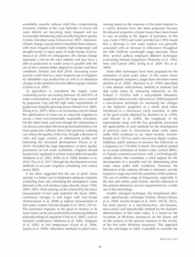
availability severely reduces yield thus compromisingeconomic viability of the crop. Episodes of severe soilwater deficits are becoming more frequent and areincreasingly threatening yield and affecting berry qualityin many viticulture areas (Chaves et al. 2007). Moreover,climate change is projected to exacerbate these impacts,with more frequent and extreme high temperature anddrought events in many parts of South Europe (Garcıa-Mozo et al. 2010). In consequence, the climate changerepresents a risk for the wine industry and may force ashift of production to cooler areas in parallel with theuse of new varieties better adapted to warmer and dryerconditions (Schultz and Stoll 2010). Increasing waterscarcity could lead to a more frequent use of irrigationfor affordable crop productivity as well as to importantchanges in the optimum areas for different grape varieties(Chaves et al. 2007).

As agriculture is considered the largest waterconsuming sector (accounting between 50 and 85% ofwater consumption), and given the large areas coveredby grapevine crop and the high water requirements ofgrapevines along the growing season (Netzer et al. 2005,Zhang et al. 2007), there is an increasing concern aboutthe optimization of water use in vineyards irrigation tosecure a more environmentally sustainable viticulture.On the other hand, and even though the relationship isnot always coincident, the most generalized tendency formain grapevine cultivars shows that generous wateringcan reduce the quality of the fruit, through a decrease incolor and sugar content, an imbalanced acidity andinterfering the flavonoid development (Flexas et al.2010). Provided the large dependence of berry qualityparameters on soil water availability, irrigation shouldbe precisely regulated to achieve reasonable fruit quality(Medrano et al. 2003, Keller et al. 2008, Romero et al.2010, Pou et al. 2011) through the development of newmethods of accurate irrigation scheduling and control(Jones 2004).

It has been suggested that the use of plant ‘stresssensing’ is a better way to implement adequate irrigationscheduling than only estimating the atmospheric waterdemand or the soil moisture status directly (Jones 1990,2004, 2007). Plant sensing can be achieved by the directmeasurement of leaf water potential (�) (Jones 2004),continuous changes in leaf turgor with leaf-clamps(Zimmermann et al. 2008) or indirect measurement ofleaf water content (Sancho-Knapik et al. 2010, 2011a).The functional response of the plant in relation to itswater status can be also predicted by monitoring differentplant physiological responses (Cifre et al. 2005), such asstomatal conductance (Medrano et al. 2002, Vilagrosaet al. 2003) or leaf temperature (Grant et al. 2006,Suarez et al. 2009). Alternative methods for plant stress

sensing based on the response of the plant material toa certain stimulus have also been proposed, becausethe physical properties of plant tissues have been foundto vary according to the degree of hydration. In thisway, Carter (1991) and Carter and McCain (1993) foundthat a decrease in leaf water content was generallyassociated with an increase in reflectance throughoutthe 400–2500 nm wavelength range spectrum. Sincethen, several authors employed different techniquesconcerning infrared frequencies (Penuelas et al. 1993,Sims and Gamon 2003, Seelig et al. 2009, Wu et al.2009).

Some other techniques have been proposed for theestimation of plant water status. In this sense, lowerelectromagnetic frequency ranges have also been tested(Jordens et al. 2009). Martınez et al. (1995) describeda time domain reflectometry method to estimate leafdisk water status by measuring reflectivity on theX-band (7–12 GHz) with a non-portable laboratoryequipment. More recently, Menzel et al. (2009) proposeda non-invasive technique for measuring the changesin the dielectric properties of a whole plant whenintroduced in a microwave cavity resonator. In spiteof the good results obtained by Martınez et al. (1995)and Menzel et al. (2009), the complexity of theexperimental setup and the low portability preventedthe applicability of such methods for the developmentof practical tools to characterize plant water statusunder field conditions so far. More recently, Sancho-Knapik et al. (2011a) used a microwave digital cordlesstelephony patch antenna to measure the reflectivity ata frequency of 1730 MHz (L-band). The method yieldedan accurate estimation of relative water content (RWC)in Populus euramericana leaves with a technologicallysimple device that constitutes a solid support for thedevelopment of a portable tool for determining plantwater status under field conditions. However, thedimension of the antenna (80 mm in diameter) and thefrequency range may limit the usefulness of this antenna.The use of another range of frequencies, especially inthe free and widely used S-band, and the reduction ofthe antenna dimension are two requirements for a wideruse of this technology.

Another emergent technique, the broad-band ultra-sonic spectroscopy technique (Gomez Alvarez-Arenaset al. 2009, Sancho-Knapik et al. 2010, 2011b, 2012),has been proven as a non-destructive, non-invasive,non-contact and reproducible method for the dynamicdetermination of leaf water status. It is based on theexcitation of thickness resonances on the leaves andon the analysis of the spectral response in the vicinityof the first order thickness resonance. This approachhas the advantage to make it possible to consider the

Physiol. Plant. 2012

VI

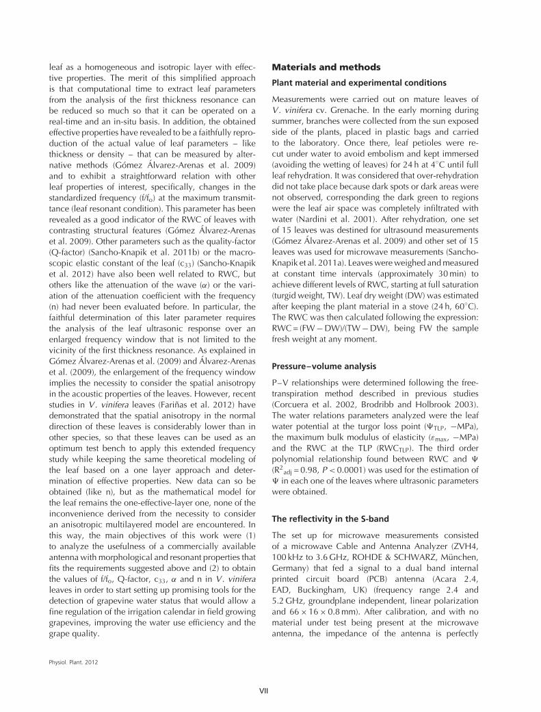
leaf as a homogeneous and isotropic layer with effec-tive properties. The merit of this simplified approachis that computational time to extract leaf parametersfrom the analysis of the first thickness resonance canbe reduced so much so that it can be operated on areal-time and an in-situ basis. In addition, the obtainedeffective properties have revealed to be a faithfully repro-duction of the actual value of leaf parameters – likethickness or density – that can be measured by alter-native methods (Gomez Alvarez-Arenas et al. 2009)and to exhibit a straightforward relation with otherleaf properties of interest, specifically, changes in thestandardized frequency (f/fo) at the maximum transmit-tance (leaf resonant condition). This parameter has beenrevealed as a good indicator of the RWC of leaves withcontrasting structural features (Gomez Alvarez-Arenaset al. 2009). Other parameters such as the quality-factor(Q-factor) (Sancho-Knapik et al. 2011b) or the macro-scopic elastic constant of the leaf (c33) (Sancho-Knapiket al. 2012) have also been well related to RWC, butothers like the attenuation of the wave (α) or the vari-ation of the attenuation coefficient with the frequency(n) had never been evaluated before. In particular, thefaithful determination of this later parameter requiresthe analysis of the leaf ultrasonic response over anenlarged frequency window that is not limited to thevicinity of the first thickness resonance. As explained inGomez Alvarez-Arenas et al. (2009) and Alvarez-Arenaset al. (2009), the enlargement of the frequency windowimplies the necessity to consider the spatial anisotropyin the acoustic properties of the leaves. However, recentstudies in V. vinifera leaves (Farinas et al. 2012) havedemonstrated that the spatial anisotropy in the normaldirection of these leaves is considerably lower than inother species, so that these leaves can be used as anoptimum test bench to apply this extended frequencystudy while keeping the same theoretical modeling ofthe leaf based on a one layer approach and deter-mination of effective properties. New data can so beobtained (like n), but as the mathematical model forthe leaf remains the one-effective-layer one, none of theinconvenience derived from the necessity to consideran anisotropic multilayered model are encountered. Inthis way, the main objectives of this work were (1)to analyze the usefulness of a commercially availableantenna with morphological and resonant properties thatfits the requirements suggested above and (2) to obtainthe values of f/fo, Q-factor, c33, α and n in V. viniferaleaves in order to start setting up promising tools for thedetection of grapevine water status that would allow afine regulation of the irrigation calendar in field growinggrapevines, improving the water use efficiency and thegrape quality.

Materials and methods

Plant material and experimental conditions

Measurements were carried out on mature leaves ofV. vinifera cv. Grenache. In the early morning duringsummer, branches were collected from the sun exposedside of the plants, placed in plastic bags and carriedto the laboratory. Once there, leaf petioles were re-cut under water to avoid embolism and kept immersed(avoiding the wetting of leaves) for 24 h at 4◦C until fullleaf rehydration. It was considered that over-rehydrationdid not take place because dark spots or dark areas werenot observed, corresponding the dark green to regionswere the leaf air space was completely infiltrated withwater (Nardini et al. 2001). After rehydration, one setof 15 leaves was destined for ultrasound measurements(Gomez Alvarez-Arenas et al. 2009) and other set of 15leaves was used for microwave measurements (Sancho-Knapik et al. 2011a). Leaves were weighed and measuredat constant time intervals (approximately 30 min) toachieve different levels of RWC, starting at full saturation(turgid weight, TW). Leaf dry weight (DW) was estimatedafter keeping the plant material in a stove (24 h, 60◦C).The RWC was then calculated following the expression:RWC = (FW − DW)/(TW − DW), being FW the samplefresh weight at any moment.

Pressure–volume analysis

P–V relationships were determined following the free-transpiration method described in previous studies(Corcuera et al. 2002, Brodribb and Holbrook 2003).The water relations parameters analyzed were the leafwater potential at the turgor loss point (�TLP, −MPa),the maximum bulk modulus of elasticity (εmax, −MPa)and the RWC at the TLP (RWCTLP). The third orderpolynomial relationship found between RWC and �

(R2adj = 0.98, P < 0.0001) was used for the estimation of

� in each one of the leaves where ultrasonic parameterswere obtained.

The reflectivity in the S-band

The set up for microwave measurements consistedof a microwave Cable and Antenna Analyzer (ZVH4,100 kHz to 3.6 GHz, ROHDE & SCHWARZ, Munchen,Germany) that fed a signal to a dual band internalprinted circuit board (PCB) antenna (Acara 2.4,EAD, Buckingham, UK) (frequency range 2.4 and5.2 GHz, groundplane independent, linear polarizationand 66 × 16 × 0.8 mm). After calibration, and with nomaterial under test being present at the microwaveantenna, the impedance of the antenna is perfectly

Physiol. Plant. 2012

VII

matched to the main circuitry. Under this condition,no electrical wave reflections occur within the circuitry.The presence of water at the vicinity of the antenna,however, alters the antenna’s impedance. The resultingmismatch of impedances is produced by inserting a thintissue (the leaf) with a different dielectric constant fromthe one the antenna was designed for (air). The valueof the sample dielectric constant is highly influencedby its water content (Martınez et al. 1995), so thecorresponding reflectivity coefficient will be a directfunction of the amount of water being present at or nearthe antenna (Sancho-Knapik et al. 2011a).

With the antenna device, we measured on each leafand at different RWC levels the relationship between themicrowave frequency (from 2.25 to 2.55 GHz) and themagnitude (dB). After all the measurements were done,we analyzed which range of frequencies had a bettercorrelation with the values of RWC. For this range, wecalculated the existing area (S) between the curve fullhydrated (RWC = 1) and another single curve (RWC = i)following the next equation:

Si =x=a∑

x=b

(MgRWC=1 (x) − MgRWC=i (x)

)(1)

where a and b are the start and the end values of thefrequency range and Mg is the magnitude (dB). Once Swas obtained, it was directly correlated with RWC.

The broadband ultrasonic spectroscopy technique

The broadband ultrasonic spectroscopy techniqueis well described and schematically depicted inGomez Alvarez-Arenas (2003a) and Sancho-Knapiket al. (2010, 2011b). Briefly, the experimental set-upconsists of two pairs of specially designed air-coupledpiezoelectric transducers working at a frequency rangeof 0.3–1.2 MHz, and with a radiating diameter areaof 20 mm (Gomez Alvarez-Arenas 2003a, 2004). Thesetransducers are positioned facing each other at a distanceof 2 cm. A high voltage (100–400 V) square semicycle(duration of 0.67 µs) is applied with a Panametrics5077 pulser-receiver (Olympus, Center Valley, PA) tothe transmitter transducer that converts this electricalsignal into an ultrasonic pulse and launches it intothe air. The receiver transducer collects this signaland converts it into an electrical one, then it isamplified (up to 59 dB) and filtered (low-pass filter at10 MHz). Eventually, an oscilloscope (Tektronix 5052TDS, Tektronix Inc., Beaverton, OR) digitizes it, averagesa number of waveforms to reduce the high frequencynoise (typically up to 100 waveforms), performs the fastFourier transform and transfers the data to a computer

for storage and further calculations. The experimentalprocedure of the ultrasonic technique is as follows.First, transmission from a transmitter is directly measuredinto the receiver, providing a calibration of the system.Then a leaf is held for a few seconds between thetransducers at normal incidence. When the ultrasoundsimpact normally on the leaf surface, part of the energyis transmitted through the leaf, and reaches the backsurface. Then part of the energy is transmitted throughthe interface (air) and received at the receiver transducer.The major modification of the approach here proposed isto consider a frequency band that not only considers thevicinity of the first thickness resonance, but a frequencywindow as large as possible considering restrictions inthe frequency band of the ultrasonic sensors. For thispurpose, measuring frequency window was set from 0.3to 1.2 MHz.

The parameters directly measured were the magnitudeand the phase of the transmission coefficient in thefrequency domain (Sancho-Knapik et al. 2012). Then, inreal time, the values of the resonant frequency (f), qualityfactor (Q), attenuation coefficient (α), macroscopiceffective elastic constant in the leaf thickness direction(c33) and the variation of the attenuation coefficient withthe frequency (n) of the leaf were calculated followingthe procedure described in Sancho-Knapik et al. (2012),being afterwards related to RWC. Each single valueof f was divided by the maximum value obtained atRWC = 1.00 (fo) for each leaf, calculating, in this way,the standardized frequency (f/fo) associated with themaximum transmittance at the peak curve (Sancho-Knapik et al. 2011b). The Q factor was defined as theratio between the resonance frequency and the widthof the resonance peak measured at 3 dB below themaximum value (Gomez Alvarez-Arenas 2003b). Theinverse of the quality factor (1/Q) was employed, because1/Q is directly related to the attenuation coefficient (α).An increase in 1/Q or in α reflects either an increase inthe irregularity of the acoustic pathway (increase in thenumber of scatterers: cavitation) or an increase of therelative influence on energy conversion mechanisms (i.e.variation of heat generation by alteration of the influenceof the friction between different tissues or by differentcomponents of the same tissue). The macroscopiceffective elastic constant of the leaf, c33, relates thecompressional deformation in the thickness directionwith the stress applied in the same direction; it isgiven in MPa (Landau and Lifshitz 1959). To describethe variation of the attenuation coefficient with thefrequency, a power law is considered, see Eqn 1, wherethe parameter n is used as a measure of this variation:

α = α0fn (2)

Physiol. Plant. 2012

VIII

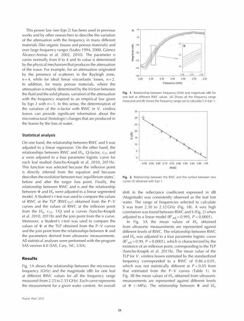
This power law (see Eqn 2) has been used in previousworks and by other researchers to describe the variationof the attenuation with the frequency in many differentmaterials (like organic tissues and porous materials) andover large frequency ranges (Szabo 1994, 2000, GomezAlvarez-Arenas et al. 2002, 2010). The parameter nvaries normally from 0 to 4 and its value is determinedby the physical mechanism that produces the attenuationof the wave. For example, for an attenuation originatedby the presence of scatterers in the Rayleigh zone,n = 4, while for ideal linear viscoelastic losses, n = 2.In addition, for many porous materials, where theattenuation is mainly determined by the friction betweenthe fluid and the solid phases, variation of the attenuationwith the frequency respond to an empirical law givenby Eqn 2 with n = 1. In this sense, the determination ofthe variation of the n-factor with RWC in V. viniferaleaves can provide significant information about themicrostructural (histologic) changes that are produced inthe leaves by the loss of water.

Statistical analysis

On one hand, the relationship between RWC and S wasadjusted to a linear regression. On the other hand, therelationships between RWC and f/fo, Q-factor, c33 andα were adjusted to a four parameter logistic curve foreach leaf studied (Sancho-Knapik et al. 2010, 2011b).This function was selected because the inflexion pointis directly inferred from the equation and becausedescribes the evolution between two ‘equilibrium states’,before and after the turgor loss point. Finally, therelationship between RWC and n and the relationshipbetween � and f/fo were adjusted to a linear segmentedmodel. A Student’s t-test was used to compare the valuesof RWC at the TLP (RWCTLP) obtained from the P–Vcurves and the values of RWC at the inflexion pointfrom the f/fo, c33, 1/Q and α curves (Sancho-Knapiket al. 2010, 2011b) and the join point from the n curve.Moreover, a Student’s t-test was used to compare thevalues of � at the TLP obtained from the P–V curvesand the join point from the relationships between � andthe parameters derived from ultrasonic measurements.All statistical analyses were performed with the programSAS version 8.0 (SAS, Cary, NC, USA).

Results

Fig. 1A shows the relationship between the microwavefrequency (GHz) and the magnitude (dB) for one leafat different RWC values for all the frequency rangemeasured (from 2.25 to 2.55 GHz). Each curve representsthe measurement for a given water content. An overall

A

B

Fig. 1. Relationship between frequency (GHz) and magnitude (dB) forone leaf at different RWC values. (A) Shows all the frequency rangemeasured and (B) shows the frequency range use to calculate S in Eqn 1.

Fig. 2. Relationship between the RWC and the surface between twocurves (S) obtained with Eqn 1.

shift in the reflectance coefficient expressed in dB(Magnitude) was consistently observed as the leaf lostwater. The range of frequencies selected to calculateS was from 2.30 to 2.32 GHz (Fig. 1B). A very highcorrelation was found between RWC and S (Fig. 2) whenadjusted to a linear model (R2

adj = 0.995, P < 0.0001).In Fig. 3A the mean values of f/fo obtained

from ultrasonic measurements are represented againstdifferent levels of RWC. The relationship between RWCand f/fo was adjusted to a four parameter logistic curve(R2

adj = 0.99, P < 0.0001), which is characterized by theexistence of an inflexion point, corresponding to the TLP(Sancho-Knapik et al. 2011b). The mean value of theTLP for V. vinifera leaves estimated by the standardizedfrequency corresponded to a RWC of 0.86 ± 0.01,which was not statistically different at P < 0.05 fromthat estimated from the P–V curves (Table 1). InFig. 3B the mean values of f/fo obtained from ultrasonicmeasurements are represented against different levelsof � (−MPa). The relationship between � and f/fo

Physiol. Plant. 2012

IX

A

B

Fig. 3. Relationships between the standardized frequency (f/fo) and theRWC (A) and the water potential (�, −MPa) (B) for Vitis vinifera cv.Grenache leaves.

Table 1. Parameters derived from the P–V curves for Vitis vinifera cv.Grenache: water potential at the turgor loss point (�TLP, −MPa), relativewater content at the turgor loss point (RWCTLP) and the maximum bulkmodulus of elasticity (εmax, −MPa). Data are expressed as mean ± SE of10 leaves.

P–V parameters V . vinifera cv. Grenache

�TLP (−MPa) 1.99 ± 0.03RWCTLP 0.85 ± 0.01εmax (−MPa) 11.91 ± 0.28

was adjusted to a linear segmented model (R2adj = 0.92,

P < 0.0001), which is characterized by the existenceof a join point at a � value of −1.92 ± 0.04 MPa. Thisvalue was not statistically different at P < 0.05 from �TLP

estimated from the P–V curves (Table 1).Fig. 4 shows the relationships between RWC and

the mean values of macroscopic elastic constant of theleaf in the Z direction (c33), the inverse of the qualityfactor of the leaf first thickness resonance (1/Q), theattenuation of the leaf first thickness resonance (α) andthe mean values of the variation of the attenuationcoefficient with the frequency (n). The relationshipsbetween RWC and c33, 1/Q and α were also adjustedto a four parameter logistic curve (R2

adj = 0.960, 0.988

and 0.988, respectively; P < 0.0001). The mean valueof the TLP for V. vinifera leaves estimated by c33 wasnot statistically different at P < 0.05 from that estimatedfrom the P–V curves (Table 1), whereas the TLP derivedfrom 1/Q and α measurements were slightly lower. Therelationship between RWC and n was adjusted to a linearsegmented model (R2

adj = 0.966, P < 0.0001), which ischaracterized by the existence of a join point at a RWCvalue of 0.80 ± 0.02.

Discussion

The large water requirements of V. vinifera duringthe growing season (Netzer et al. 2005, Zhang et al.2007) implies the need for irrigation in the driest areasof its distribution range to avoid constraints on thephotosynthetic activity due to stomatal closure (Flexaset al. 1998, Chaves et al. 2010). The stomatal behaviorin grapevine has been proposed as characteristic of adrought-avoiding, isohydric plant (Zufferey et al. 2011).Thus, the reduction in transpiration regulates the xylemtension, limiting the risks of a hydraulic failure bycavitation (Cochard et al. 2002, Brodribb et al. 2003,Choat et al. 2010). However, more recently, Zuffereyet al. (2011) have proposed that stomatal closure inV. vinifera cannot regulate by itself the risk of drought-induced cavitation, proposing that the diurnal cyclesof cavitation and refilling in the petioles act as a‘hydraulic fuse’ that exacerbate the ability for reachingrisky water potential in the whole water pathway. Thehigh vulnerability found for leaf petioles (estimatedthrough the water potential at which plants lose 50%of hydraulic conductivity, PLC50 < −1.0 MPa) reportedin this article indicates the extreme sensitivity of theleaves in this plant species to small changes in leaf waterpotential, as long as the existence of this ‘hydraulic fuse’preserves the leaf from further consequences in termsof whole plant hydraulics but reduces the capability forkeeping certain levels of photosynthesis. The triggeringof this ‘hydraulic fuse’ in this species occurs when thewater potential is well above the TLP measured here(approximately −2 MPa, Table 1) and those reported byAlsina et al. (2007) for several grapevine cultivars. Thisfact implies that drastic changes in the leaf physiologicalperformance of V. vinifera would happen in a verynarrow water potential range.

Among the different methods that have been usedfor the estimation of the leaf water status, the use ofthe reflectance in the infrared region of the spectrum,especially in the so-called ‘water bands’ (Carter 1991,Penuelas et al. 1993, Seelig et al. 2009), faces theproblem of the strong influence of the leaf thicknesschanges at positive turgor pressures (Sancho-Knapik

Physiol. Plant. 2012

X

A B

C D

Fig. 4. Relationship between the RWC and the macroscopic effective elastic constant (c33) (A), the inverse of Q-factor (1/Q) (B), the attenuation ofthe leaf first thickness resonance (α, m−1) (C) and the variation of the attenuation coefficient with the frequency (n) (D) for Vitis vinifera cv. Grenacheleaves. Data are expressed as mean ± SE of 15 leaves.

et al. 2011a). Effectively, these authors confirmed thatthe leaf experiences a marked decrease in thicknessuntil the turgor is lost, which counteracts the changesin reflectance values due to leaf water losses (Seeliget al. 2009). On the other hand, the ‘pressure-probe’ developed by Zimmermann et al. (2008), whichmeasures changes in turgor pressure in intact leaves,and the estimation of reflectivity at the L-band with amicrowave antenna (Sancho-Knapik et al. 2011a) canalso serve as a tool for the detection of changes in theleaf water content above the turgor loss point. However,both methods imply a close contact between the deviceand the leaf surface, which in a long time recording canderive in leaf bleaching and other problems.

The measure of the reflectance at a frequency closeto 2.4 GHz gives an estimation of the changes in thedielectric property of the leaves as the water contentdecreases (Martinez et al. 1995). The good correlationsfound between the parameter S (see Eqn 1) and theRWC in V. vinifera suggest a promising use of thistechnique in this species, especially in combination withthe physiological information given by the ultrasonicmethod (Sancho-Knapik et al. 2011b). The new antennatested in this article improves the benefits of the one used

by Sancho-Knapik et al. (2011a), both in dimensions,commercial availability and frequency range.

The air-coupled broadband ultrasonic spectroscopyallows the determination of leaf water status in anon-contact and non-invasive way, which constitutes anoteworthy progress with respect to the other techniquesabove mentioned. Among the different variables thatcan be registered, the frequency associated with themaximum transmittance (f/fo) is an optimum parameterfor the estimation of plant water status above the TLPin V. vinifera (Fig. 3A). Moreover, the changes foundin the macroscopic elastic constant of the leaf in the Zdirection (c33), which is known to be dependent on thefrequency (Sancho-Knapik et al. 2011b), were highlycorrelated with changes in RWC, particularly before theTLP (Fig. 4A). Finally, the variation of the attenuationcoefficient with the frequency (n) strongly decreasedwith the RWC at positive turgor pressures (Fig. 4D). Thedetermination of this parameter can only be achievedby considering the extension of the frequency windowanalysis proposed in this work. This extension canquestion the applicability of the one-layer effectivemedium acoustic model used to extract the propertiesof the leaf from the measured spectra. As a matter of

Physiol. Plant. 2012

XI

fact, this model can only be done if the anisotropybetween the different leaf layers in the thicknessdirection can be considered negligible. Availableevidences suggest that grapevine leaves can be soconsidered. Election of V. vinifera leaves is critical inthis point because of the low attenuation in these leavesas compared with other species. For example, whileattenuation in V. vinifera leaves is about 800 Np m−1

at 0.6 MHz, attenuation coefficient (extrapolated atthe same frequency) for other species is 1200 Np m−1

(Epipremnum aureum), 1600–1800 Np m−1 (Prunuslaurocerasus), 800–1500 Np m−1 (Ligustrum lucidum),2000–3000 Np m−1 (Platanus hispanica) and1300–1400 Np m−1 (Populus × euramericana) (GomezAlvarez-Arenas et al. 2009, Farinas et al. 2012).Thanks to this relatively lower attenuation coefficient ingrapevine leaves, measuring frequency window can beset to the 0.3–1.2 MHz range, which is large enough toget a faithful estimation of the parameter n. In addition,the variation found in n may suggest that the mainsource of ultrasonic attenuation varies from scatteringby small scatterers (n close to 4) to viscoelastic losses(n close to 2). Further investigations are required tocorrelate these variations of the dominant mechanismof ultrasonic losses with histological variations inthe leaves. Although these three variables accuratelydefined the RWC of this species above the turgorloss point, n was the parameter that showed a greatpercentage of variation of the dynamic range duringthis phase (ca. 62%), when compared with f/fo, (ca.45%) and c33 (ca. 50%). In this sense, it is worthwhileto note that while f/fo, and c33 are determined by theelasticity of the leaf, 1/Q, α and n are determined bythe various mechanisms that produce the attenuation ofthe ultrasonic wave: presence of scatterers and energyconversion phenomena. Therefore it is possible toobserve a different evolution of these parameters whenthe leaf RWC or water potential varies depending onhow this variation may affect the leaf microstructure andhow these changes affect the different factors involvedin setting up the ultrasonic response of the leaf.

Otherwise, the air-coupled broadband ultrasonicspectroscopy can be used for the determination of theTLP in V. vinifera. Effectively, no significant differenceswere found between the RWCTLP derived from analy-sis of P–V isotherms and those obtained by calculatingthe inflexion point in the RWC vs f/fo and c33 rela-tionships, respectively, which was previously reportedby Sancho-Knapik et al. (2012) in L. lucidum, Pop-ulus × euramericana and Platanus × hispanica and P.laurocerasus. The accumulation of evidences suggeststhat the use of ultrasonic measurements would consti-tute a valuable tool for assessing the turgor loss in plant

species. Recently, Bartlett et al. (2012) have revisitedthe ecological importance of the TLP in terms of waterpotential as a major physiological determinant of plantwater stress response. In case this parameter, rather thanthe RWC at zero turgor, is preferable the use of the rela-tionship between � and f/fo can also be used (Fig. 3B).Once TLP is overpassed, the different ultrasonic vari-ables are also well informative about the changes in thewater status of V. vinifera leaves. In this phase, a shift inthe parameters directly related to the attenuation of thesignal (α, 1/Q) was observed (Fig. 4B, C). However, 1/Qand n are not optimum to quantitatively monitor plantwater status once turgor is lost (when RWC is below 0.85)because of the large scattering in the signal. For this RWCrange, c33 and α could constitute a better way for a moreaccurate estimation of water status in grapevine leaves.A substantial improvement in the accuracy of RWC esti-mation below TLP can be achieved by a simultaneoususe of both ultrasounds and microwave parameters.

In conclusion, this study has proven that the twotechniques here presented can be suitable for theestimation of the leaf water status in V. vinifera throughthe different phases experienced by the leaves in thedehydration process. The measurement of reflectanceat frequencies close to 2.4 GHz gives an excellentaccuracy when the changes in S are correlated withthe value of RWC. The information given by the air-coupled broad band ultrasonic spectroscopy does notlie on one single variable, yielding information fromdifferent and non-redundant parameters, which allowsfor a more convincing knowledge of the water status inthis plant species. The combined use of both techniquesand the development of single and portable device forusing these methods under field conditions constitute achallenge that deserves further efforts.

Acknowledgements – This study was partially supported bythe projects AGL2010-21153-C02-02 (Ministerio de Cien-cia e Innovacion, Spain) and DPI2011-22438 (Ministerio deEconomıa y Competitividad, Spain). Financial support fromGobierno de Aragon (A54 research group) is also acknowl-edged. Work of J. J. P.-P. is supported by a ‘‘Juan de laCierva’’-MICIIN post-doctoral contract.

References

Alsina MM, De Herralde F, Aranda X, Save R, Biel C(2007) Water relations and vulnerability to embolismare not related: experiments with eight grapevinecultivars. Vitis 46: 1–6

Alvarez-Arenas TG, Sancho-Knapik D, Peguero-Pina JJ,Gil-Pelegrın E (2009) Determination of plant leaveswater status using air-coupled ultrasounds. Proceedingsof the IEEE Ultrasonics Symp, Rome, pp 771–774

Physiol. Plant. 2012XII

Bartlett MK, Scoffoni C, Sack L (2012) The determinants ofleaf turgor loss point and prediction of drought toleranceof species and biomes: a global meta-analysis. Ecol Lett15: 393–405

Brodribb TJ, Holbrook NM (2003) Stomatal closure duringleaf dehydration, correlation with other leafphysiological traits. Plant Physiol 132: 2166–2173

Brodribb TJ, Holbrook NM, Edward EJ, Gutierrez MV(2003) Relations between stomatal closure, leaf turgorand xylem vulnerability in eight tropical dry forest trees.Plant Cell Environ 26: 443–450

Carter GA (1991) Primary and secondary effects of watercontent on the spectral reflectance of leaves. Am J Bot78: 916–924

Carter GA, McCain DG (1993) Relationship of leaf spectralreflectance to chloroplast water content determinedusing NMR microscopy. Remote Sens Environ 46:305–310

Chaves MM, Santos TP, Souza CR, Ortuno MF, RodriguesML, Lopes CM, Maroco JP, Pereira JS (2007) Deficitirrigation in grapevine improves water-use efficiencywhile controlling vigour and production quality. AnnAppl Biol 150: 237–252

Chaves MM, Zarrouk O, Francisco R, Costa JM, Santos T,Regalado AP, Rodrigues ML, Lopes CM (2010)Grapevine under deficit irrigation: hints fromphysiological and molecular data. Ann Bot 105:661–676

Choat B, Drayton WM, Brodersen CR, Matthews MA,Shackel KA, Wada H, McElrone AJ (2010) Measurementof vulnerability to water stress-induced cavitation ingrapevine: a comparison of four techniques applied tolong-vesseled species. Plant Cell Environ 33:1502–1512

Cifre J, Bota J, Escalona JM, Medrano H, Flexas J (2005)Physiological tools for irrigation scheduling in grapevine(Vitis vinifera L.). An open gate to improve water-useefficiency? Agric Ecosyst Environ 105(2–3): 159–170

Cochard H, Coll L, Le Roux X, Ameglio T (2002)Unraveling the effects of plant hydraulics on stomatalclosure during water stress in walnut. Plant Physiol 128:282–290

Corcuera L, Camarero JJ, Gil-Pelegrın E (2002) Functionalgroups in Quercus species derived from the analysis ofpressure–volume curves. Trees 16: 465–472

Farinas MD, Sancho-Knapik D, Peguero-Pina JJ,Gil-Pelegrın E, Alvarez-Arenas TG (2012) Shear wavesin plant leaves at ultrasonic frequencies: shearproperties of vegetal tissues. Proceedings of the IEEEUltrasonics Symp, Dresden, in press

Flexas J, Escalona JM, Medrano H (1998) Down-regulationof photosynthesis by drought under field conditions ingrapevine leaves. Aust J Plant Physiol 25: 893–900

Flexas J, Galmes J, Galle A, Gulıas J, Pou A, Ribas-CarboM, Tomas M, Medrano H (2010) Improvement of water

use efficiency in grapevines. Aust J Grape Wine Res 16:106–121

Garcıa-Mozo H, Mestre A, Galan C (2010) Phenologicaltrends in southern Spain: a response to climate change.Agric For Meteorol 150: 575–580

Gomez Alvarez-Arenas TE (2003a) Air-coupled ultrasonicspectroscopy for the study of membrane filters. J MembrSci 213: 195–207

Gomez Alvarez-Arenas TE (2003b) A non-destructiveintegrity test for membrane filters based on air-coupledultrasonic spectroscopy. IEEE Trans Ultrason FerroelectrFreq Control 50: 676–685

Gomez Alvarez-Arenas TE (2004) Acoustic impedancematching of piezoelectric transducers to the air. IEEETrans Ultrason Ferroelectr Freq Control 51: 624–633

Gomez Alvarez-Arenas TE, Montero F, Moner M,Rodrıguez E, Roig A, Molins E (2002) Viscoelasticity ofsilica aerogels at ultrasonic frequencies. Appl Phys Lett81: 1198–1200

Gomez Alvarez-Arenas TE, Sancho-Knapik D,Peguero-Pina JJ, Gil-Pelegrın E (2009) Noncontact andnoninvasive study of plant leaves using air-coupledultrasounds. Appl Phys Lett 95: 193702

Gomez Alvarez-Arenas TE, Calas H, Ealo-Cuello J,Ramos-Fernandez A, Munoz M (2010) Noncontactultrasonic spectroscopy applied to the study ofpolypropylene ferroelectrets. J Appl Phys 108: 074110

Grant OM, Tronina L, Chaves MM (2006) Exploringthermal imaging variables for the detection of stressresponses in grapevine under different irrigationregimes. J Exp Bot 58: 815–825

Jones HG (1990) Plant water relations and implications forirrigation scheduling. Acta Hortic 278: 67–76

Jones HG (2004) Irrigation scheduling: advantages andpitfalls of plant-based methods. J Exp Bot 55:2427–2436

Jones HG (2007) Monitoring plant and soil water status:established and novel methods revisited and theirrelevance to studies of drought tolerance. J Exp Bot 58:119–130

Jordens C, Scheller M, Breitenstein B, Selmar D, Koch M(2009) Evaluation of leaf water status by means ofpermittivity at terahertz frequencies. J Biol Phys 35:255–264

Keller M, Smithyman RP, Mills LJ (2008) Interactive effectsof deficit irrigation and crop load on CabernetSauvignon in an arid climate. Am J Enol Vitic 59:221–234

Landau LD, Lifshitz EM (1959) Theory of elasticity. Courseof theoretical physics, Vol. 7. Pergamon Press, Oxford,UK

Martınez M, Artacho JM, Fornies-Marquina JM, Letosa J,Garcıa-Gracia M, Gil E (1995) Dielectric behaviour byT.D.R. of the water status in a vegetal leaf. OHDBiennial Colloquium Digest 13: 330–333

Physiol. Plant. 2012

XIII

Medrano H, Escalona JM, Bota J, Gulıas J, Flexas J (2002)Regulation of photosynthesis of C3 plants in response toprogressive drought: the interest of stomatalconductance as a reference parameter. Ann Bot 89:895–905

Medrano H, Escalona JM, Cifre J, Bota J, Flexas J (2003) Aten-year study on the physiology of two Spanishgrapevine cultivars under field conditions: effects ofwater availability from leaf photosynthesis to grape yieldand quality. Funct Plant Biol 30: 607–619

Menzel MI, Tittmann S, Buhler J, Preis S, Wolters N, JahnkeS, Walter A, Chlubek A, Leon A, Hermes N, OffenhauserA, Gilmer F, Blumler P, Schurr U, Krause HJ (2009)Non-invasive determination of plant biomass withmicrowave resonators. Plant Cell Environ 32: 368–379

Nardini A, Tyree MT, Salleo S (2001) Xylem cavitation inthe leaf of Prunus laurocerasus and its impact on leafhydraulics. Plant Physiol 125: 1700–1709

Netzer Y, Yao C, Shenker M, Bravdo B, Schwartz A, CohenS (2005) Water consumption of ‘‘superior’’ grapevinesgrown in a semiarid region. Acta Hortic 689: 399–405

Penuelas J, Filella I, Biel C, Serrano L, Save R (1993) Thereflectance at the 950–970 nm region as indicator ofplant water status. Int J Remote Sens 14: 1887–1905

Pou A, Gulias J, Moreno M, Tomas M, Medrano H, Cifre J(2011) Cover cropping in Vitis vinifera L. cv MantoNegro vineyards under Mediterranean conditions:effects on plant vigour, yield and grape quality. J Int SciVigne Vin 45: 223–234

Romero P, Fernandez-Fernandez JI, Martınez-Cutillas A(2010) Physiological thresholds for efficient regulateddeficit-irrigation management in winegrapes grownunder semiarid conditions. Am. J Enol Vitic 61: 300–312

Sancho-Knapik D, Gomez Alvarez-Arenas T, Peguero-PinaJJ, Gil-Pelegrın E (2010) Air-coupled broadbandultrasonic spectroscopy as a new non-invasive andnon-contact method for the determination of leaf waterstatus. J Exp Bot 61: 1385–1391

Sancho-Knapik D, Gismero J, Asensio A, Peguero-Pina JJ,Fernandez V, Gomez Alvarez-Arenas T, Gil-Pelegrın E(2011a) Microwave L-band (1730 MHz) accuratelyestimates the relative water content in poplar leaves. Acomparison with a near infrared water index(R1300/R1450). Agric For Meteorol 151: 827–832

Sancho-Knapik D, Gomez Alvarez-Arenas T, Peguero-PinaJJ, Fernandez V, Gil-Pelegrın E (2011b) Relationshipbetween ultrasonic properties and structural changes inthe mesophyll during leaf dehydration. J Exp Bot 62:3637–3645

Sancho-Knapik D, Calas H, Peguero-Pina JJ,Ramos-Fernandez A, Gil-Pelegrın E, GomezAlvarez-Arenas T (2012) Air-coupled ultrasonic resonant

spectroscopy for the study of the relationship betweenplant leaves’ elasticity and their water content. IEEETrans Ultrason Ferroelectr Freq Control 59: 319–325

Schultz HR, Stoll M (2010) Some critical issues inenvironmental physiology of grapevines: futurechallenges and current limitations. Aust J Grape WineRes 16: 4–24

Seelig HD, Hoehn A, Stodieck LS, Klaus DM, Adams WWIII, Emery WJ (2009) Plant water parameters and theremote sensing R1300/R1450 leaf water index: controlledcondition dynamics during the development of waterdeficit stress. Irrigation Sci 27: 357–365

Sims DA, Gamon JA (2003) Estimation of vegetation watercontent and photosynthetic tissue area from spectralreflectance: a comparison of indices based on liquidwater and chlorophyll absorption features. Remote SensEnviron 84: 526–537

Suarez L, Zarco-Tejada PJ, Berni JAJ, Gonzalez-Dugo V,Fereres E (2009) Modelling PRI for water stress detectionusing radiative transfer models. Remote Sens Environ113: 730–744

Szabo TL (1994) Time domain wave equations for lossymedia obeying a frequency power law. J Acoust Soc Am96: 491–500

Szabo TL (2000) A model for longitudinal and shear wavepropagation in viscoelastic media. J Acoust Soc Am 107:2437–2446

Tonietto J, Carbonneau A (2004) A multicriteria climaticclassification system for grape-growing regionsworldwide. Agric For Meteorol 124: 81–97

Vilagrosa A, Bellot J, Vallejo VR, Gil-Pelegrın E (2003)Cavitation, stomatal conductance, and leaf dieback inseedlings of two co-occurring Mediterranean shrubsduring an intense drought. J Exp Bot 54: 2015–2024

Wu C, Niu Z, Tang Q, Huang W (2009) Predictingvegetation water content in wheat using normalizeddifference water indices derived from groundmeasurements. J Plant Res 122: 317–326

Zhang BZ, Kang SZ, Zhang L, Du TS, Li SE, Yang XY(2007) Estimation of seasonal crop water consumptionin a vineyard using Bowen ratio-energy balancemethods. Hydrol Processes 21: 3635–3641

Zimmermann D, Reuss R, Westhoff M, Gebner P, BauerW, Bamberg E, Bentrup FW, Zimmermann U (2008) Anovel, non-invasive, online-monitoring, versatile andeasy plant-based probe for measuring leaf water status. JExp Bot 59: 3157–3167

Zufferey V, Cochard H, Ameglio T, Spring JL, Viret O(2011) Diurnal cycles of embolism formation and repairin petioles of grapevine (Vitis vinifera cv. Chasselas). JExp Bot 62: 3885–3894

Edited by J. Flexas

Physiol. Plant. 2012

XIV

© The Author 2013. Published by Oxford University Press. All rights reserved. For Permissions, please email: journals.permissions@oup.com

Tree Physiology 33, 695–700doi:10.1093/treephys/tpt052

Ultrasonic spectroscopy allows a rapid determination of the relative water content at the turgor loss point: a comparison with pressure–volume curves in 13 woody species

Domingo Sancho-Knapik1, José Javier Peguero-Pina2, María Dolores Fariñas3, Tomás Gómez Álvarez-Arenas3 and Eustaquio Gil-Pelegrín1,4

1Unidad de Recursos Forestales, Centro de Investigación y Tecnología Agroalimentaria, Gobierno de Aragón, 50059, Zaragoza, Spain; 2Departament de Biologia, Universitat de les Illes Balears, Carretera de Valldemossa, 07071, Palma de Mallorca, Spain; 3Ultrasound for Medical and Industrial Applications (UMEDIA) Research Group, Centre for Physical Technologies, C.S.I.C., 28002, Madrid, Spain; 4Corresponding author (egilp@aragon.es)

Received April 18, 2013; accepted July 1, 2013; handling Editor Frederick Meinzer

The turgor loss point (TLP), which is considered a threshold for many physiological processes, may be useful in plant-breed-ing programs or for the selection of reforestation species. Obtaining TLP through the standard pressure–volume (p–v) curve method in a large set of species is highly time-consuming and somewhat subjective. To solve this problem, we present an objective and a less time-consuming technique based on the leaf resonance able to calculate the relative water content (RWC) at TLP (RWCTLP). This method uses air-coupled broadband ultrasonic spectroscopy to obtain the sigmoidal relation between RWC and the standardized resonant frequency (f/fo). For the 13 species measured, the inflexion point of the RWC–f/fo relation-ship (RWCTLP of f/ ) was not statistically different from the value of RWC at the TLP obtained with the p–v curves (RWCTLP p–v).

Keywords: drought, relative water content, turgor loss point, ultrasonic spectroscopy.

Introduction

The turgor loss point (TLP) has been considered a threshold for many physiological processes (e.g., Franks et al. 1995, Brodribb and Holbrook 2003, Thomas et al. 2006, Mitchell et al. 2008). A drop in turgor has been associated with stoma-tal closure (Brodribb and Holbrook 2003), inhibition of photo-synthesis (Lawlor and Cornic 2002; Brodribb and Holbrook 2003, Bartlett et al. 2012b), plant growth (Frensch and Hsiao 1994) or with other responses of plants to water-limiting con-ditions (Mitchell et al. 2008). Therefore, the determination of the specific TLP provides information on the ability of the plant to withstand different stress conditions while maintaining ade-quate physiological activity.

Leaf TLP is generally estimated from pressure–volume (p–v) curves, which relate the decrease of leaf water potential (Ψ)

with the leaf relative water content (RWC) (Tyree and Hammel 1972). The TLP is defined as the point where the p–v curve transitions from a non-linear to a linear relationship (Turner 1988). In this way, the TLP can be defined in terms of water potential (ΨTLP) or in terms of RWC (RWCTLP). While many stud-ies have focused on ΨTLP, many others have provided evidence for the outstanding importance of RWCTLP in physiological and ecological studies. Some authors have shown different values of RWCTLP in different populations from the same species (Jane and Green 1983; Wan et al. 1998). Others have found different values within a single species depending on the treatment imposed (White et al. 1996, Gucci et al. 1997, Bacelar et al. 2006). Seasonal changes in RWCTLP have also been reported (Kubiske and Abrams 1991, White et al. 2000). Furthermore, several studies have found interspecific differences in RWCTLP with values of RWCTLP being generally higher in mesic than in

Technical note

by guest on October 14, 2013

http://treephys.oxfordjournals.org/D

ownloaded from

by guest on O

ctober 14, 2013http://treephys.oxfordjournals.org/

Dow

nloaded from

by guest on October 14, 2013

http://treephys.oxfordjournals.org/D

ownloaded from

by guest on O

ctober 14, 2013http://treephys.oxfordjournals.org/

Dow

nloaded from

by guest on October 14, 2013

http://treephys.oxfordjournals.org/D

ownloaded from

by guest on O

ctober 14, 2013http://treephys.oxfordjournals.org/

Dow

nloaded from

XV

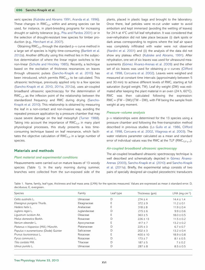
Tree Physiology Volume 33, 2013

xeric species (Kubiske and Abrams 1991, Aranda et al. 1996). These changes in RWCTLP within and among species can be used, for instance, in plant-breeding programs for increasing drought or salinity tolerance (e.g., Pita and Pardos 2001) or in the selection of drought-resistant tree species for timber pro-duction (e.g., Merchant et al. 2007).

Obtaining RWCTLP through the standard p–v curve method in a large set of species is highly time-consuming (Bartlett et al. 2012a). Another difficulty using this method lies in the subjec-tive determination of where the linear region switches to the non-linear (Schulte and Hinckley 1985). Recently, a technique based on the excitation of thickness resonances on leaves through ultrasonic pulses (Sancho-Knapik et al. 2010) has been introduced, which permits RWCTLP to be calculated. This ultrasonic technique, previously applied only to a few species (Sancho-Knapik et al. 2010, 2011a, 2012a), uses air-coupled broadband ultrasonic spectroscopy for the determination of RWCTLP as the inflexion point of the relationship between the standardized frequency and RWC during drying (Sancho-Knapik et al. 2010). This relationship is obtained by measuring the leaf in a non-contact and non-invasive way, avoiding the repeated pressure application by a pressure chamber that may cause severe damage on the leaf mesophyll (Turner 1988). Taking into account the importance of RWCTLP in many plant physiological processes, this study presents a less time- consuming technique based on leaf resonance, which facili-tates the objective calculation of RWCTLP in a large number of species.

Materials and methods

Plant material and experimental conditions

Measurements were carried out on mature leaves of 13 woody species (Table 1). In the early morning during summer, branches were collected from the sun-exposed side of the

plants, placed in plastic bags and brought to the laboratory. Once there, leaf petioles were re-cut under water to avoid embolism and kept immersed (avoiding the wetting of leaves) for 24 h at 4°C until full leaf rehydration. It was considered that over-rehydration did not take place because (i) dark spots or dark areas corresponding to regions where the leaf air space was completely infiltrated with water were not observed (Nardini et al. 2001) and (ii) the analysis of the data did not show any plateau effect (Kubiske and Abrams, 1991). After rehydration, one set of six leaves was used for ultrasound mea-surements (Gómez Álvarez-Arenas et al. 2009) and the other set of six leaves was used for obtaining p–v curves (Clifford et al. 1998, Corcuera et al. 2002). Leaves were weighed and measured at constant time intervals (approximately between 5 and 30 min) to achieve different levels of RWC, starting at full saturation (turgid weight, TW). Leaf dry weight (DW) was esti-mated after keeping the plant material in an oven (24 h, 60°C). RWC was then calculated following the expression: RWC = (FW − DW)/(TW − DW), with FW being the sample fresh weight at any moment.

Pressure–volume analysis

p–v relationships were determined for the 13 species using a pressure chamber and following the free-transpiration method described in previous studies (Lo Gullo et al. 1986, Clifford et al. 1998, Corcuera et al. 2002, Vilagrosa et al. 2003). The water relations parameter calculated as a mean and standard error of individual values was the RWC at the TLP (RWCTLP p–v).

Air-coupled broadband ultrasonic spectroscopy

The air-coupled broadband ultrasonic spectroscopy technique is well described and schematically depicted in Gómez Álvarez-Arenas (2003), Sancho-Knapik et al. (2010) and Sancho-Knapik et al. (2011a). Briefly, the experimental setup consists of two pairs of specially designed air-coupled piezoelectric transducers

696 Sancho-Knapik et al.

Table 1. Name, family, leaf type, thickness and leaf mass area (LMA) for the species measured. Values are expressed as mean ± standard error. D, deciduous; E, evergreen.

Species Family Leaf type Thickness (µm) LMA (mg cm−2)

Celtis australis L. Ulmaceae D 274 ± 4 14.4 ± 1.4Elaeagnus pungens Thunb. Eleagnaceae E 372 ± 9 11.2 ± 0.1Hedera helix L. Araliaceae E 318 ± 8 11.9 ± 0.4Juglans regia L. Juglandaceae D 215 ± 6 9.9 ± 0.6Ligustrum lucidum Ait. Oleaceae E 363 ± 5 18.0 ± 0.5Malus domestica Borkh. Rosaceae D 226 ± 13 11.5 ± 0.2Nerium oleander L. Apocynaceae E 417 ± 7 13.2 ± 0.2Platanus × hispanica (Mill.) Münchh. Platanaceae D 225 ± 3 6.7 ± 0.7Populus × euramericana (Dode) Guinier Salicaceae D 202 ± 3 13.2 ± 0.4Prunus laurocerasus L. Rosaceae E 400 ± 10 18.9 ± 0.8Pyrus communis L. Rosaceae D 173 ± 7 8.1 ± 0.5Tilia cordata Mill. Tiliaceae D 187 ± 5 7 ± 0.2Ulmus pumila L. Ulmaceae D 287 ± 8 8.5 ± 0.5

XVI

Tree Physiology Online at http://www.treephys.oxfordjournals.org

working at a frequency range of 0.3–1.2 MHz, and with a radiat-ing diameter area of 20 mm (Gómez Álvarez-Arenas 2003, 2004). These transducers are positioned facing each other at a distance of 2 cm. A high-voltage (100–400 V) square semi cycle (duration of 0.67 µs) is applied with a Panametrics 5077 pulser-receiver (Olympus, Center Valley, PA, USA) to the transmitter transducer which converts this electrical signal into an ultrasonic pulse and launches it into the air. The receiver transducer collects this signal and converts it into an electrical one, then it is ampli-fied (up to 59 dB) and filtered (low-pass filter at 10 MHz). Eventually, an oscilloscope (Tektronix 5052 TDS, Tektronix Inc., Beaverton, OR, USA) digitizes it, averaging a number of wave-forms to reduce the high-frequency noise (typically up to 100 waveforms), performing the fast Fourier transform and transfer-ring the data to a computer for storage. The experimental proce-dure for the ultrasonic technique is as follows. First, the transmission from a transmitter is directly measured into the receiver, providing a calibration of the system. Then, a leaf is held for a few seconds between the transducers at normal incidence. When the ultrasonic pulses impact normally on the leaf surface, a part of the energy is transmitted through the leaf reaching the back surface. Then, a part of the energy is transmitted through the interface (air) and received at the receiver transducer.

The parameter directly measured from the ultrasound spec-troscopy technique was the magnitude of the transmission coefficient in the frequency domain (Sancho-Knapik et al. 2010). Then, in real time, the values of the resonant frequency (f) of the leaf were calculated following the proceduredescribed in Sancho-Knapik et al. (2012b), being related toRWC afterward. Each single value of f was divided by the maxi-mum value obtained at RWC = 1.00 (fo) for each leaf, calculat-ing, in this way, the standardized frequency (f/fo) associatedwith the maximum transmittance at the peak curve (Sancho-Knapik et al. 2011a). The relationship between RWC and f/fowas adjusted to a four-parameter logistic curve (f = a + (b − a)/(1 + (RWC/c)d)) for each leaf studied (Sancho-Knapik et al.2010, 2011a). This function was selected because the inflex-ion point (coefficient c) is objectively inferred from the equa-tion and because it describes the evolution between two‘equilibrium states’, before and after the TLP.

Statistical analysis

A Student’s t-test was used to compare the values of RWCTLP obtained from the p–v curves (RWCTLP p–v) and the values of RWC at the inflexion point of the standardized frequency curves (RWCTLP of f/ ) (Sancho-Knapik et al. 2010, 2011a, 2012b). Furthermore, for all species, the mean values of RWCTLP obtained with p–v curves were plotted against the mean values obtained through ultrasounds. This relation was adjusted to a linear regression and compared through an analysis of variance against a y = x regression. All statistical analyses were performed with the program SAS version 8.0 (SAS, Cary, NC, USA).

Results

The values of TLP in terms of RWC (RWCTLP p–v) obtained from the p–v curves ranged from 0.771 ± 0.007 (Ulmus pumila L.) to 0.909 ± 0.006 (Elaeagnus pungens Thunb.). The Student’s t-test (at α = 0.05 and α = 0.01) did not show any significantdifference between RWCTLP p–v values and those obtained fromthe ultrasound technique (RWCTLP of f/ ). Moreover, if the meanvalues were plotted against each other, RWCTLP p–v againstRWCTLP of f/ (Figure 1), its linear regression (R2 = 0.99) was notstatistically different (α = 0.01) from the linear function y = x,indicating that the slope was not statistically significantly differ-ent from 1 and the intercepts were not statistically differentfrom zero at the 99% confidence level.

The relationship between mean values of RWC and f/fo obtained through the ultrasonic technique is shown in Figure 2 for four species (E. pungens, Juglans regia L., Pyrus communis L., U. pumila). For comparison, the relationship between mean values of RWC and 1/Ψ has been added in each graph. It is observed in all cases that the point where the non-linear part of the RWC–1/Ψ relationship switches to a straight line (marked in Figure 2 with a shadow rectangle) matches in terms of RWC with the inflexion point of the sigmoidal curve of the RWC–f/fo relation. This can be observed both in the species with the lower TLP (U. pumila) as well as in those having a higher TLP (E. pungens).

Discussion

The various techniques which were used to measure water sta-tus in plant science and their suitability for different purposes have been widely reviewed during the last decade (Jones 2007). New tools and techniques have been gradually

Ultrasonic determination of the turgor loss point 697

Figure 1. Relationship and linear regression between the RWC at the TLP obtained with p–v curves (RWCTLP p–v) and with ultrasonic measure-ments (RWCTLP of f/ ) for the species measured. Values are expressed asmean ± standard error.

XVII

Tree Physiology Volume 33, 2013

introduced to achieve better estimations of plant water status (Geitmann 2006, Grant et al. 2006, Sepulcre-Canto et al. 2007, Peguero-Pina et al. 2008, Zimmermann et al. 2008, Sancho-Knapik et al. 2010, 2011b, Bartlett et al. 2012a). As a consequence, the contribution of new measuring procedures may help us improve our understanding of plant water relations.

As a new technique, air-coupled broadband ultrasonic spec-troscopy has been reported to be useful for the estimation of the RWC at the TLP in some previous studies (Sancho-Knapik et al. 2010, 2011a, 2012a). However, a maximum of only two species per study were utilized, pointing to the necessity of incorporating results from a wider range of plant species (Sancho-Knapik et al. 2010). In the present study, the ultra-sonic technique has been demonstrated to be an objective method for the determination of the TLP in 13 different species (Table 1). It is interesting to note that the species analyzed comprised a wide range of RWCTLP: from 0.771 to 0.909. For

all species, there were no statistically significant differences between the values of RWCTLP derived from the analysis of p–v isotherms and those obtained as the inflexion point of the rela-tionships between RWC and f/fo. Therefore, we are able to affirm that the TLP in terms of RWC can be accurately esti-mated through the calculation of the inflexion point of the RWC–f/fo relationship.

The main advantages of this procedure, as compared with the classical analysis of the p–v isotherms (Tyree and Hammel 1972, Corcuera et al. 2002), are the reduced time consump-tion and objectivity. With the ultrasound technique, the leaf is held between the transducers and the measurement takes not more than few seconds. Using a pressure chamber implies the handling of the chamber and repeated pressurizations and slow releases of pressure, each of which can take several min-utes at lower water potentials (Turner, 1988). On the other hand, RWCTLP is objectively obtained with the ultrasonic tech-nique, whereas the determination of RWCTLP from p–v curves

698 Sancho-Knapik et al.

Figure 2. Relationships between mean values of RWC and standardized frequency (f/fo) obtained through the ultrasonic technique (white circles) and relationships between mean values of RWC and the inverse of water potential (1/Ψ) obtained with the p–v curves (gray and black circles) for E. pungens, J. regia, P. communis and U. pumila. Gray circles correspond to values of RWC above TLP and black circles correspond to values of RWCbelow TLP which are chosen for the linear regression. The shaded rectangle marks the TLP on both relationships. Values are expressed asmean ± standard error.

XVIII

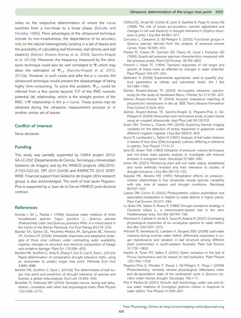
Tree Physiology Online at http://www.treephys.oxfordjournals.org

relies on the subjective determination of where the curve switches from a non-linear to a linear phase (Schulte and Hinckley 1985). More advantages of the ultrasound technique include its non-invasiveness, the dependence of its accuracy only on the natural heterogeneity existing in a set of leaves and the possibility of calculating leaf thickness, leaf density and leaf elasticity (Gómez Álvarez-Arenas et al. 2009, Sancho-Knapik et al. 2012b). Moreover, the frequency measured by the ultra-sonic technique could also be well correlated to Ψ, which may allow the estimation of ΨTLP (Sancho-Knapik et al. 2010, 2012a). However, in such cases and alike the p–v curves, the ultrasound technique would present the disadvantage of being highly time-consuming. To solve this problem, ΨTLP could be inferred from a few points beyond TLP of the RWC–osmotic potential (π) relationship, which is the straight portion of the RWC–1/Ψ relationship in the p–v curve. These points may be obtained during the ultrasonic measurement process or in another similar set of leaves.

Conflict of interest

None declared.

Funding

This study was partially supported by CAIXA project 2012/GA-LC-002 (Departamento de Ciencia, Tecnología y Universidad, Gobierno de Aragón) and by the MINECO projects |AGL2010-21153-C02-02, DPI 2011-22438 and INNPACTO 2012 SOST-WINE. Financial support from Gobierno de Aragón (A54 research group) is also acknowledged. The work of José Javier Peguero-Pina is supported by a ‘Juan de la Cierva’-MINECO post-doctoral contract.

References

Aranda I, Gil L, Pardos J (1996) Seasonal water relations of three broadleaved species Fagus sylvatica L., Quercus petraea (Mattuschka) Liebl. and Quercus pyrenaica Willd. in a mixed stand in the centre of the Iberian Peninsula. For Ecol Manag 84:219–229.

Bacelar EA, Santos DL, Moutinho-Pereira JM, Gonçalves BC, Ferreira HF, Correia CM (2006) Immediate responses and adaptative strate-gies of three olive cultivars under contrasting water availability regimes: changes on structure and chemical composition of foliage and oxidative damage. Plant Sci 170:596–605.

Bartlett MK, Scoffoni C, Ardy R, Zhang Y, Sun S, Cao K, Sack L (2012a) Rapid determination of comparative drought tolerance traits: using an osmometer to predict turgor loss point. Methods Ecol Evol 3:880–888.

Bartlett MK, Scoffoni C, Sack L (2012b) The determinants of leaf tur-gor loss point and prediction of drought tolerance of species and biomes: a global meta-analysis. Ecol Lett 15:393–405.

Brodribb TJ, Holbrook NM (2003) Stomatal closure during leaf dehy-dration, correlation with other leaf physiological traits. Plant Physiol 132:2166–2173.

Clifford SC, Arndt SK, Corlett JE, Joshi S, Sankhla N, Popp M, Jones HG (1998) The role of solute accumulation, osmotic adjustment and changes in cell wall elasticity in drought tolerance in Ziziphus mauri-tiana (Lamk). J Exp Bot 49:967–977.

Corcuera L, Camarero JJ, Gil-Pelegrin E (2002) Functional groups in Quercus species derived from the analysis of pressure–volume curves. Trees 16:465–472.

Franks PJ, Cowan IR, Tyerman SD, Cleary AI, Lloyd J, Farquhar GD (1995) Guard-cell pressure aperture characteristics measured with the pressure probe. Plant Cell Environ 18:795–800.

Frensch J, Hsiao TC (1994) Transient responses of cell turgor and growth of maize roots as affected by changes in water potential. Plant Physiol 104:247–254.

Geitmann A (2006) Experimental approaches used to quantify phy-sical parameters at cellular and subcellular levels. Am J Bot 93:1380–1390.

Gómez Álvarez-Arenas TE (2003) Air-coupled ultrasonic spectro-scopy for the study of membrane filters. J Membr Sci 213:195–207.

Gómez Álvarez-Arenas TE (2004) Acoustic impedance matching of piezoelectric transducers to the air. IEEE Trans Ultrason Ferroelectr Freq Control 51:624–633.

Gómez Álvarez-Arenas TE, Sancho-Knapik D, Peguero-Pina JJ, Gil-Pelegrin E (2009) Noncontact and noninvasive study of plant leaves using air-coupled ultrasounds. Appl Phys Lett 95:193702.

Grant OM, Tronina L, Chaves MM (2006) Exploring thermal imaging variables for the detection of stress responses in grapevine under different irrigation regimes. J Exp Bot 58:815–825.

Gucci R, Lombardini L, Tattini M (1997) Analysis of leaf water relations in leaves of two olive (Olea europaea) cultivars differing in tolerance to salinity. Tree Physiol 17:13–21.

Jane GT, Green TGA (1983) Utilisation of pressure–volume techniques and non-linear least squares analysis to investigate site induced stresses in evergreen trees. Oecologia 57:380–390.

Jones HG (2007) Monitoring plant and soil water status: established and novel methods revisited and their relevance to studies of drought tolerance. J Exp Bot 58:119–130.

Kubiske ME, Abrams MD (1991) Rehydration effects on pressure– volume relationships in four temperate woody species: variability with site, time of season and drought conditions. Oecologia 85:537–542.

Lawlor DW, Cornic G (2002) Photosynthetic carbon assimilation and associated metabolism in relation to water deficits in higher plants. Plant Cell Environ 25:275–294.

Lo Gullo MA, Salleo S, Rosso R (1986) Drought avoidance strategy in Ceratonia siliqua L., a mesomorphic-leaved tree in the xeric Mediterranean area. Ann Bot 58:745–756.

Merchant A, Callister A, Arndt S, Tausz M, Adams M (2007) Contrasting physiological responses of six eucalyptus species to water deficit. Ann Bot 100:1507–1515.

Mitchell PJ, Veneklaas EJ, Lambers H, Burgess SSO (2008) Leaf water relations during summer water deficit: differential responses in tur-gor maintenance and variation in leaf structure among different plant communities in south-western Australia. Plant Cell Environ 31:1791–1802.

Nardini A, Tyree MT, Salleo S (2001) Xylem cavitation in the leaf of Prunus laurocerasus and its impact on leaf hydraulics. Plant Physiol 125:1700–1709.

Peguero-Pina JJ, Morales F, Flexas J, Gil-Pelegrín E, Moya I (2008) Photochemistry, remotely sensed physiological reflectance index and de-epoxidation state of the xanthophyll cycle in Quercus coc-cifera under intense drought. Oecologia 156:1–11.

Pita P, Pardos JA (2001) Growth, leaf morphology, water use and tis-sue water relations of Eucalyptus globulus clones in response to water deficit. Tree Physiol 21:599–607.

Ultrasonic determination of the turgor loss point 699

XIX

Tree Physiology Volume 33, 2013

Sancho-Knapik D, Gómez Álvarez-Arenas T, Peguero-Pina JJ, Gil-Pelegrin E (2010) Air-coupled broadband ultrasonic spectroscopy as a new non-invasive and non-contact method for the determina-tion of leaf water status. J Exp Bot 61:1385–1391.

Sancho-Knapik D, Gómez Álvarez-Arenas T, Peguero-Pina JJ, Fernandez V, Gil-Pelegrin E (2011a) Relationship between ultra-sonic properties and structural changes in the mesophyll during leaf dehydration. J Exp Bot 62:3637–3645.

Sancho-Knapik D, Gismero J, Asensio A, Peguero-Pina JJ, Fernández V, Gómez Álvarez-Arenas T, Gil-Pelegrín E (2011b) Microwave L-band (1730 MHz) accurately estimates the relative water content in pop-lar leaves. A comparison with a near infrared water index (R1300/R1450). Agric For Meteorol 151:827–832.

Sancho-Knapik D, Peguero-Pina JJ, Medrano H, Fariñas MD, Gómez Álvarez-Arenas T, Gil-Pelegrin E (2012a) The reflectivity in the S-band and the broadband ultrasonic spectroscopy as new tools forthe study of water relations in Vitis vinifera L. Physiol Plant148:512–521.

Sancho-Knapik D, Calas H, Peguero-Pina JJ, Ramos-Fernandez A, Gil-Pelegrin E, Gómez Álvarez-Arenas T (2012b) Air-coupled ultrasonic resonant spectroscopy for the study of the relationship between plant leaves’ elasticity and their water content. IEEE Trans Ultrason Ferroelectr Freq Control 59:319–325.

Schulte PJ, Hinckley TM (1985) A comparison of pressure–volume curve data analysis techniques. J Exp Bot 36:1590–1602.

Sepulcre-Canto G, Zarco-Tejada PJ, Jimenez-Munoz JC, Sobrino JA, Soriano MA, Fereres E, Vega V, Pastor M (2007) Monitoring yield and fruit quality parameters in open-canopy tree crops under

water stress. Implications for ASTER. Remote Sens Environ 107:455–470.

Thomas TR, Matthews MA, Shackel KA (2006) Direct in situ measure-ment of cell turgor in grape (Vitis vinifera L.) berries during develop-ment and in response to plant water deficits. Plant Cell Environ 29:993–1001.

Turner NC (1988) Measurement of plant water status by pressure chamber technique. Irrigation Sci 9:289–308.

Tyree MT, Hammel HT (1972) Measurement of turgor pressure and water relations of plants by pressure bomb technique. J Exp Bot 23:267–282.

Vilagrosa A, Bellot J, Vallejo VR, Gil-Pelegrin E (2003) Cavitation, sto-matal conductance, and leaf dieback in seedlings of two cooccur-ring Mediterranean shrubs during an intense drought. J Exp Bot 54:2015–2024.

Wan C, Sosebee RE, McMichael BL (1998) Water relations and root growth of two populations of Gutierrezia sarothrae. Environ Exp Bot 39:11–20.

White DA, Beadle CL, Worledge D (1996) Leaf water relations of Eucalyptus globulus ssp. globulus and E. nitens: seasonal, drought and species effects. Tree Physiol 16:469–476.

White DA, Turner NC, Galbraith JH (2000) Leaf water relations and stomatal behaviour of four allopatric Eucalyptus species planted in Mediterranean southwestern Australia. Tree Physiol 20:1157–1165.

Zimmermann D, Reuss R, Westhoff Gebner P, Bauer W, Bamberg Bentrup FW, Zimmermann U (2008) A novel, noninvasive, online-monitoring, versatile and easy plant-based probe for measuring leaf water status. J Exp Bot 59:3157–3167.

700 Sancho-Knapik et al.

XX

ANEXO I

NC-RUS Aplicado a Materiales No Biológicos FERRARO, C., GARCIA-TUÑON, E., ROCHA, V.G., BARG, S., FARIÑAS, M.D., ALVAREZ-

ARENAS, T.E.G., SERNICOLA, G., GIULIANI, F. y SAIZ, E., 2016. Light and Strong SiC Networks. Advanced Functional Materials, vol. 26, no. 10, pp. 1636-1645. ISSN 1616301X. DOI 10.1002/adfm.201504051. Disponible en: http://onlinelibrary.wiley.com/doi/10.1002/adfm.201504051/abstract

En este artículo, se caracteriza mediante la técnica central de esta tesis doctoral una red de SiC de muy alta porosidad (92% - 98%) y rigidez y durezas superiores a la de los aerogeles de densidades similares. Este novedoso material presenta una estructura tipo panal (honeycomb) jerarquizado y dispuesto en capas. El coeficiente de transmisión en incidencia normal fue medido en ambas direcciones de propagación calculando los parámetros ultrasónicos correspondientes, los cuales reflejan su alto grado de anisotropía.

XXI

M.D. FARIÑAS, 2016

XXII

FULL P

APER

© 2016 WILEY-VCH Verlag GmbH & Co. KGaA, Weinheim 1wileyonlinelibrary.com

highly porous ceramics have been fabri-cated in macroscopic dimensions using diverse technologies such as emulsifi cation or direct foaming; however, the pore sizes are large (typically above 100 µm) and the materials tend to be weak. [ 5 ] At the other extreme, aerogels exhibit nanosized pores but are not strong. [ 7,8 ] Recent work has demonstrated the fabrication of metallic [ 9 ] and ceramic [ 1,3,4,6 ] microlattices with microsized pores and struts by combining additive manufacturing and thin fi lm deposition. They can reach remarkable mechanical properties as a result of their carefully designed architectures but their dimensions are usually small (10–10 3 µm) and to date they have been fabricated from a very limited range of materials (Al 2 O 3 and TiN). [ 1,3,4,6 ] The challenge remains on how to broaden the material palette to form strong, thermally and chemically

stable light structures in practical dimensions using fl exible, low-cost technologies for high-volume fabrication.

Silicon carbide is a very appealing material for the fabrica-tion of light structures and microlattices. It combines excellent thermal stability and shock resistance, low thermal expansion, superb mechanical strength, and high chemical stability. [ 10,11 ] As a consequence, light and porous SiC structures are of interest for a number of advanced technological applications. Commercial uses of porous silicon carbide have already been exploited for example in fi lters for water, diesel particulate, hot gas or molten metals, porous burners, metal and polymer matrix composites, high-temperature/high-voltage semicon-ductor electronics, or membranes. [ 11 ] However, these are “con-ventional” porous materials with porosities still below 80%. The development of even lighter, stiff and strong porous SiC would be extremely advantageous for many of these technologies and would open new opportunities in others.

Nature offers many examples of highly porous materials (such as bone or wood) that are light and retain toughness and strength. A common characteristic of these biological materials is their complex hierarchical architecture from the macro down to the nanoscale. [ 12 ] It has been also shown how the architecture of lattices can be manipulated to create stretching-dominated structures and increase their mechanical effi ciency. [ 6,13 ] However, when translating these structural con-cepts, it is important to remember that the strength and stiff-ness of a porous ceramic scale with those of their wall or strut.

Light and Strong SiC Networks Claudio Ferraro , Esther Garcia-Tuñon , Victoria G. Rocha , Suelen Barg , Maria Dolores Fariñas , Tomas E. Gomez Alvarez-Arenas , Giorgio Sernicola , Finn Giuliani , and Eduardo Saiz *

The directional freezing of microfi ber suspensions is used to assemble highly porous (porosities ranging between 92% and 98%) SiC networks. These networks exhibit a unique hierarchical architecture in which thin layers with honeycomb-like structure and internal strut length in the order of 1–10 µm in size are aligned with an interlayer spacing ranging between 15 and 50 µm. The resulting structures exhibit strengths (up to 3 MPa) and stiffness (up to 0.3 GPa) that are higher than aerogels of similar density and comparable to other ceramic microlattices fabricated by vapor deposition. Furthermore, this wet processing technique allows the fabrication of large-size samples that are stable at high temperature, with acoustic impedance that can be manipulated over one order of magnitude (0.03–0.3 MRayl), electrically conductive and with very low thermal conductivity. The approach can be extended to other ceramic materials and opens new opportunities for the fabrication of ultra-light structures with unique mechanical and functional properties in practical dimensions.

DOI: 10.1002/adfm.201504051

C. Ferraro, Dr. E. Garcia-Tuñon, Dr. V. G. Rocha, G. Sernicola, Dr. F. Giuliani, Prof. E. Saiz Centre for Advanced Structural Ceramics Department of Materials Imperial College London South Kensington Campus London SW7 2AZ , UK E-mail: e.saiz@imperial.ac.uk Dr. S. Barg The School of Materials The University of Manchester Oxford Road , Manchester M13 9PL , UK M. D. Fariñas, Dr. T. E. G. Alvarez-Arenas Sensors and Ultrasonic Technologies Department Information and Physics Technologies Institute (ITEFI) Spanish National Research Council (CSIC) Serrano 144 , 28006 Madrid , Spain

1. Introduction

In recent years, a signifi cant effort has been devoted to the development of ultralight, highly porous ceramic structures. Their potential mechanical and functional capabilities are of interest in many advanced technologies from transportation to catalysis or tissue engineering. [ 1–6 ] To a large extent, the chal-lenge for these applications is to attain large porosities (above 90%) while maintaining the pore size in the microscopic scale and retaining strength and structural capabilities. A range of

Adv. Funct. Mater. 2016, DOI: 10.1002/adfm.201504051

www.afm-journal.dewww.MaterialsViews.com

XXIII

FULL

PAPER

2 wileyonlinelibrary.com © 2016 WILEY-VCH Verlag GmbH & Co. KGaA, Weinheim

These should be free of microdefects to enhance mechanical performance. [ 14 ] In consequence, a very appealing way to create a strong, highly porous ceramic lattice is through the con-trolled assembly of thin, strong microfi bers into complex hier-archical architectures. The assembly of complex, highly porous macroscopic structures from microfi bers remains a chal-lenge. [ 15 ] Here we address it by directionally freezing suspen-sions of SiC fi bers to assemble ceramic networks with macro-scopic dimensions, porosities above 90% and densities below 300 mg cm −3 . This approach allows the formation of lattices with layered architectures that can be manipulated by control-ling the composition of the suspension and the freezing con-ditions. The use of SiC enables the fabrication of light struc-tures that retain strength and stiffness and are stable up to high temperatures. Their pore and strut sizes along with their mechanical properties are comparable to microlattices pre-pared through thin fi lm deposition and they exhibit a unique combination of properties: they are electrically conductive, thermally insulating, and present very low acoustic impedance. The effect of the processing conditions on the architecture is evaluated and the mechanical and thermal properties of the networks are compared with other ceramic materials of similar densities and with existing models.

2. Results

Freeze casting of ceramics is based on the directional freezing of a suspension. As the ice grows it expels the ceramic par-ticles that accumulate in the space between ice crystals ( Figure 1 ). After sublimating the water is possible to obtain a porous ceramic whose porosity has been templated by the ice. In order to obtain a homogeneous structure the suspension should remain stable during freezing. However, due to their dimensions (diameter ≈1.5 µm, average length of ≈18 µm) the SiC fi bers can sediment rapidly resulting in inhomoge-neous materials. To avoid this problem, chitosan was used to prepare homogeneous and stable slurries. The hydroxyl and amine groups present in the repeating unit of the chitosan chain interact with the silanol groups formed on the SiC sur-face in the presence of water through hydrogen bonding. [ 16 ] These interactions along with the electrostatic forces between the chitosan chains and the SiC surfaces result in weakly fl oc-culated suspensions. Flocculation hampers sedimentation enabling the formation of homogeneous structures. By direc-tionally freezing the suspension, we promote the formation of lamellar ice that expels the fi bers as it grows. Although fl oc-culation due to chitosan increases the viscosity, it remains low enough to allow the formation of large, lamellar ice crystals (the apparent viscosity is well below 100 Pa s for fi ber con-tents up to 20 wt%). As the fi bers pack in the layers between the growing ice crystals they form a microporous network (Figure 1 ). After removing the ice template via freeze drying, we obtain a highly porous network (an irregular microlattice) with a layered architecture and macroscopic dimensions (sizes up to centimeters).

After drying, the sample is thermally treated to sinter the individual fi bers and consolidate the structure. Sintering takes place in a graphite furnace at 1800 °C under argon fl ow. To

promote pressureless sintering Al 2 O 3 and Y 2 O 3 are added to the slurry (up to 15 wt% of the SiC content). [ 17 ] These addi-tives in combination with the silica present on the SiC sur-face promote the formation of liquid at high temperature. The liquid phase enhances mass transport and facilitates fi ber–fi ber bonding (Figure 1 d). To achieve this goal and avoid the evaporation of additives at high temperature a tight control of the atmosphere is maintained by placing the sample in a closed graphite crucible, on a SiC/Al 2 O 3 powder bed. Chitosan is also expelled from the growing ice crystals during freezing and subsequently eliminated during sintering. [ 18 ] The sintered lattices exhibit a structure with highly interconnected porosity and a hierarchical architecture (Figure 1 ) formed by aligned, thin and highly porous ceramic layers. The SiC fi bers form the network struts and the architecture can be manipulated by controlling the freezing conditions and the composition of the suspension. In particular, the fi nal density of the material is determined by the solid concentration in the suspension and the distance between layers by the speed of the ice front and also the solid concentration. This separation can vary between 15 and 50 µm. As it has been observed in other systems, faster speeds result in smaller interlayer distances. [ 19 ] The wall thick-ness remains constant and of the order of the fi ber diameter (Figure 1 b). The length of the struts inside the walls varies between 1 and 10 µm. By reducing the solid loading of the suspension from 7 to 1.5 vol%, the porosity increases from 92% up to 98%. Some fi bers are trapped by the growing ice crystals during freezing and arrange perpendicularly to the lamellae forming bridges between them (Figure 1 d). The number of bridges increases with increasing fi ber concentra-tion in the starting suspensions and as a result the structure of denser lattices transitions toward a more isotropic, cellular architecture (Figure 1 ).

The combination of high porosity with the intrinsic proper-ties of SiC results on the formation of structures that are both electrically conductive (conductivities ranging from 5.3 × 10 −6 to 3.8 × 10 −4 S cm −1 ) and thermally insulating (thermal conductivi-ties of the order of 0.1–0.6 W m −1 K −1 ). There is a slight depend-ence of the thermal conductivity with the orientation for sam-ples with higher porosity ( Figure 2 ). This anisotropy could also be observed in the electrical conductivity that can be between two and six times larger in the direction parallel to the layers. Conductivity is approximately three times larger in the direction parallel to the layers for samples with a porosity of 97%. During the measurements the samples remained stable up to 1500 °C. The thermal conductivity also remained relatively stable (although it increases slightly for samples with larger pores).

The structures fail in a brittle manner under compression. As it is usually observed in brittle porous materials, the stress/strain curve reaches a plateau. [ 14 ] In this plateau, it is possible to observe dips corresponding to failure events. However, the strength is recovered after each dip ( Figure 3 ). The in situ mechanical tests in the scanning electron microscopy (SEM) revealed that when the scaffolds reach their crushing strength, the junctions between fi bers at the top and the bottom of the lattice (in contact with the plates of the testing machine) start to break and the fi bers accumulate (Figure 3 ). Wall failure at the top or bottom of the sample causes the observed dips in stress at the plateau. However, the bulk of the structure remains stable and

Adv. Funct. Mater. 2016, DOI: 10.1002/adfm.201504051

www.afm-journal.dewww.MaterialsViews.com

XXIV

FULL P

APER

3wileyonlinelibrary.com© 2016 WILEY-VCH Verlag GmbH & Co. KGaA, Weinheim

is still able to sustain the applied load. This type of behavior has been observed in other porous ceramics and microlattices. [ 4,23 ]

Anisotropy is observed in the velocity of propagation of ultra-sonic waves ( Figure 4 ). In the direction parallel to the layers they propagate between 15% and 35% faster than along the normal direction (anisotropy increases with decreasing den-sity). As expected, the ultrasound wave velocity takes very low values that increase with sample density (from 340 to 540 m s −1 for 100 mg cm −3 , up to 1100–1400 m s −1 for 250 mg cm −3 ).

Velocity values in the low range are similar to those meas-ured in silica aerogels with a similar technique. In addition, acoustic impedance can be very small (down to 0.03 MRayl) and the ultrasound attenuation coeffi cient is relatively low (50–60 Np m −1 @ 300 kHz), these values are similar to those found in conventional silica aerogels. [ 24 ] Moreover, changing the density makes possible to vary the impedance values over one order of magnitude (0.03–0.3 MRayl). This makes this kind of material a suitable candidate to produce stacks of impedance

Adv. Funct. Mater. 2016, DOI: 10.1002/adfm.201504051

www.afm-journal.dewww.MaterialsViews.com

Figure 1. a) Schematic of the freeze casting process. Lamellar ice crystals grow directionally in a fi ber water-based suspension frozen under a tem-perature gradient. The fi bers are expelled from the growing ice and form a layered structure. b) The interlayer distance, d , decreases when increasing the speed of the ice front and increasing the solid content of the suspension. c) Scanning electron image showing the layered structure of a sintered network prepared using a suspension containing 1.5 vol% fi bers (98% fi nal porosity). The inset shows how it is possible to prepare structures with macroscopic dimensions. d) Networks sintered from a 7 vol% fi ber suspension (92% fi nal porosity) showing a more isotropic structure. e) Detail of the structure shown in (c). The walls are thin (1–2 µm) and formed by entangled fi bers. Some fi bers arrange perpendicular to the walls forming bridges between them. f) Junction between fi bers showing some of the remaining liquid phase formed during sintering.

XXV

FULL

PAPER

4 wileyonlinelibrary.com © 2016 WILEY-VCH Verlag GmbH & Co. KGaA, Weinheim

matching layers for wide-band air-coupled piezoelectric trans-ducers in the low megahertz frequency range or for the realiza-tion of acoustic metamaterials. [ 25 ] There they could substitute other very low density materials (aerogels) but offering much better machinability and mechanical stability.

3. Discussion

The mechanical properties of a lattice depend on its architec-ture and the strength and modulus of the struts. In ceramic microlattices fabricated by additive manufacturing and thin

Adv. Funct. Mater. 2016, DOI: 10.1002/adfm.201504051

www.afm-journal.dewww.MaterialsViews.com

Figure 3. a) Stress–strain curves showing the brittle fracture behavior of lattices with a porosity of 94%. After reaching the compressive strength ( σ f ) the curve exhibits a plateau with dips in stress corresponding to failure events followed by a fast increase due to densifi cation. b–d) The sequence of pictures taken “in situ” in the SEM (corresponding to the continuous red line) shows how failure occurs at the junction between fi bers at the top and bottom of the sample while the center remains intact and can still hold the load. The sample can still sustain load even after a strain above 40%.

Figure 2. a) The thermal conductivities in the direction parallel (II) and perpendicular (⊥) to the layers remain low with temperature up to 1500 °C although it tends to increase at higher temperatures for the materials with larger pores. b) The thermal conductivity (room temperature values) of the SiC networks is comparable to other porous thermally insulating ceramics. Aerogels have lower thermal conductivity and are lighter but they are also weaker (data from refs. [ 20–22 ] ).

XXVI

FULL P

APER

5wileyonlinelibrary.com© 2016 WILEY-VCH Verlag GmbH & Co. KGaA, Weinheim

fi lm deposition the defect size is limited by the very thin strut walls (typically ≈10 nm thick). In consequence they can exhibit very high specifi c strengths. In addition, their geometries can be designed to avoid strut bending during compression and achieve a more effi cient relationship between mechanical response (strength and stiffness) and density. However, the pro-cessing approach limits the dimension of the lattice to few mil-limeters at most.

Here we address this problem using a bottom up fabrica-tion approach to assemble strong microscopic ceramic fi bers into macroscopic (centimeters in size) structures. The bending strength of the fi bers has been measured in situ in the scan-ning electron microscope using three-point bending. They reach values of the order of 1–3 GPa, much larger than those usually reported for sintered ceramics and comparable to those estimated for the struts of ceramic microlattices ( Figure 5 ). [ 3,4 ] Although the three-point bending tests could be overestimating

slightly the fracture strength we take this as a good indicative value for the following calculations.

The fi bers assemble into walls aligned parallel to the direc-tion of ice growth. Because fi ber assembly is not very effi cient the walls are formed by a highly porous fi ber network. This assembly process results in materials that are clearly ortho-tropic. The two dimensions perpendicular to the freezing direc-tion show similar properties compared to the third direction parallel to the freezing path. Due to the combination of strong SiC struts with a layered structure, the materials exhibit high crushing strengths and Young’s modulus in the freezing direc-tion (parallel to the walls) even at low densities ( Figure 6 ). The measured values are signifi cantly higher than aerogels and comparable to microscopic ceramic lattices with similar densi-ties fabricated using vapor deposition.

The effect of fi ber strength and lattice architecture can be discussed by comparing the expected theoretical strength and

Adv. Funct. Mater. 2016, DOI: 10.1002/adfm.201504051

www.afm-journal.dewww.MaterialsViews.com

Figure 4. a) Schematic representation of the experimental set-up to measure thickness resonances in the transmission coeffi cient of plates at normal incidence showing transmitter and receiver ultrasonic (us) transducers; and the two main directions of propagation of the ultrasonic waves in the material: along the layered microstructure and normal to it. b,c) Dots: Measured magnitude and phase spectra of the fi rst thickness resonance of the plate for plates cut along the two main directions in the material (sample 20%, 0.2 g cm −3 ); solid line: calculated response assuming the plate as an homogenous material. While for propagation along direction 1 (plate thickness 2.6 mm) the material exhibit a behavior very close to the expected one for an homogeneous material, along the direction 2 (plate thickness 1.9 mm) a sharp interference is always observed that produces a remark-able distortion of the spectra of the fi rst thickness resonance (in the case shown, at 310 kHz, see arrows). This interference can be explained by the appearance of two different guided waves that propagate along the two different and simultaneous paths of propagation that the material offers in this direction: along the layers and along the spaces between them. d) Dots: Measured magnitude and phase of the fi rst three orders of the thickness resonances for wave propagation in the direction 1; solid line: calculated response assuming the plate as a homogenous material. For this direction, material behaves as an homogeneous material in a very wide frequency band; on the contrary, for propagation in the direction 2 the spectra become distorted as frequency increases and no higher order resonances are observed.

XXVII

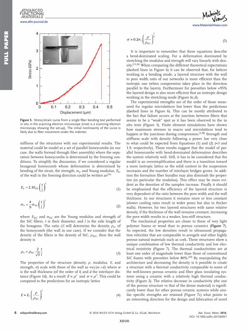
FULL

PAPER

6 wileyonlinelibrary.com © 2016 WILEY-VCH Verlag GmbH & Co. KGaA, Weinheim

stiffness of the structures with our experimental results. The material could be model as a set of parallel honeycombs (in our case, the walls formed through fi ber assembly) where the sepa-ration between honeycombs is determined by the freezing con-ditions. To simplify the discussion, if we considered a regular hexagonal honeycomb whose deformation is determined by bending of the struts, the strength, σ h , and Young modulus, E h , of the wall in the freezing direction could be written as [ 14 ]

= ⎛⎝⎜

⎞⎠⎟2.3h SiC

3

E Et

l (1)

σ σ= ⎛⎝⎜

⎞⎠⎟

4

9h SiC

2t

l (2)

where E SiC and σ SiC are the Young modulus and strength of the SiC fi bers, t is their diameter, and l is the side length of the hexagons. The ratio t / l will determine the density, ρ h , of the honeycomb (the wall in our case). If we consider that the density of the fi bers is the density of SiC, ρ SiC , then the wall density is

ρ ρ=2

3h SiC

t

l (3)

The properties of the structure (density, ρ , modulus, E , and strength, σ ) scale with those of the wall as ≈ w / (w + d) where w is the wall thickness (of the order of t ) and d the interlayer dis-tance (Figure 1 d). As a result ρ∝ 3E and σ ρ∝ 2. This could be compared to the predictions for an isotropic lattice

ρρ

≈⎛⎝⎜

⎞⎠⎟f

SiC

2

E E (4)

σ σρ

ρ≈

⎛⎝⎜

⎞⎠⎟

0.2 fSiC

32

(5)

It is important to remember that these equations describe a bend-dominated scaling. For a deformation dominated by stretching the modulus and strength will vary linearly with den-sity. [ 13,26 ] When comparing the different theoretical expectations (dashed lines in Figure 6 ) it can be observed that, for lattices working in a bending mode, a layered structure with the wall to pore width ratio of our networks is more effi cient than the isotropic one (when compression takes place in the direction parallel to the layers). Furthermore for porosities below ≈95% the layered design is also more effi cient that an isotropic design working in the stretching mode (Figure 6 c,d).

The experimental strengths are of the order of those meas-ured for regular microlattices but lower than the predictions (dashed lines in Figure 6 ). This can be mostly attributed to the fact that failure occurs at the junction between fi bers that seems to be a “weak” spot as it has been observed in the in situ tests (Figure 3 ). Finite element simulations have shown how maximum stresses in macro and microlattices tend to happen at the junctions during compression. [ 3,28 ] Strength and stiffness scale with density following a power law very close to what could be expected from Equations ( 1) and ( 2) (≈3 and 1.9, respectively). These results suggest that the model of par-allel honeycombs with bend-dominated deformation describes the system relatively well. Still, it has to be considered that the model is an oversimplifi cation and there is a transition toward a more isotropic lattice as the solid content in the suspension increases and the number of interlayer bridges grows. In addi-tion the formation fi ber bundles may also diminish the proper-ties (in particular the modulus). This effect may be more evi-dent as the densities of the samples increase. Finally it should be emphasized that the effi ciency of the layered structure is very dependent of the ratio between the pore width and the wall thickness. In our structures it remains more or less constant (slower cooling rates result in wider pores but also in thicker walls). However, for two layered structures with same relative density, if the thickness of the wall remains constant, increasing the pore width results in a weaker, less-stiff structure.

The mechanical properties are closer to those of very light polymer foams or wood than to porous ceramics ( Figure 7 ). As expected, the low densities result in ultrasound propaga-tion velocities that are comparable to aerogels and other highly porous natural materials such as cork. These structures show a unique combination of low thermal conductivity and low elec-trical resistivity (Figure 7 ). The thermal conductivities are at least one order of magnitude lower than those of conventional SiC foams with porosities below 80%. [ 29 ] By manipulating the architecture and decreasing the density is it possible to create a structure with a thermal conductivity comparable to some of the well-known porous ceramic and fi ber glass insulating sys-tems using a ceramic with a relatively high thermal conduc-tivity (Figure 2 ). The relative decrease in conductivity (the one of the porous structure vs that of the dense material) is signifi -cantly lower than for other porous ceramic systems while sim-ilar specifi c strengths are retained (Figure 7 c) what points to an interesting direction for the design and fabrication of novel

Adv. Funct. Mater. 2016, DOI: 10.1002/adfm.201504051

www.afm-journal.dewww.MaterialsViews.com

Figure 5. Stress/strain curve from a single fi ber bending test performed in situ in the scanning electron microscope (inset is a scanning electron microscopy showing the set-up). The initial nonlinearity of the curve is likely due to fi ber movement under the indenter.

XXVIII

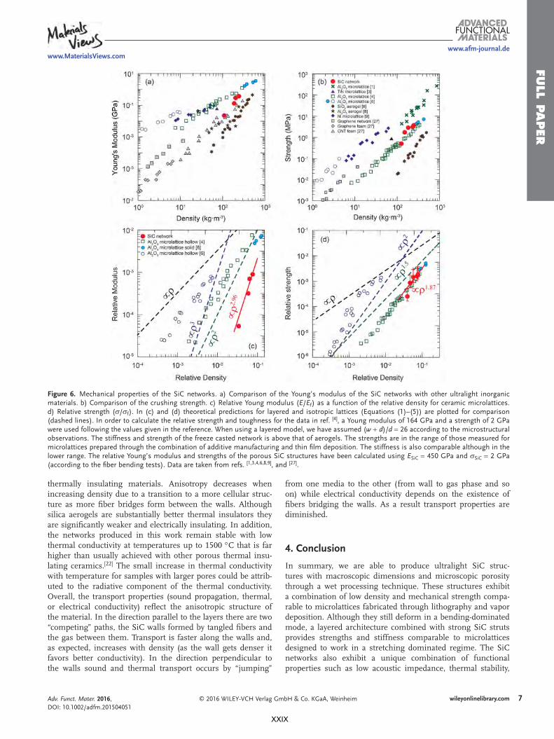
FULL P

APER

7wileyonlinelibrary.com© 2016 WILEY-VCH Verlag GmbH & Co. KGaA, Weinheim

thermally insulating materials. Anisotropy decreases when increasing density due to a transition to a more cellular struc-ture as more fi ber bridges form between the walls. Although silica aerogels are substantially better thermal insulators they are signifi cantly weaker and electrically insulating. In addition, the networks produced in this work remain stable with low thermal conductivity at temperatures up to 1500 °C that is far higher than usually achieved with other porous thermal insu-lating ceramics. [ 22 ] The small increase in thermal conductivity with temperature for samples with larger pores could be attrib-uted to the radiative component of the thermal conductivity. Overall, the transport properties (sound propagation, thermal, or electrical conductivity) refl ect the anisotropic structure of the material. In the direction parallel to the layers there are two “competing” paths, the SiC walls formed by tangled fi bers and the gas between them. Transport is faster along the walls and, as expected, increases with density (as the wall gets denser it favors better conductivity). In the direction perpendicular to the walls sound and thermal transport occurs by “jumping”

from one media to the other (from wall to gas phase and so on) while electrical conductivity depends on the existence of fi bers bridging the walls. As a result transport properties are diminished.

4. Conclusion

In summary, we are able to produce ultralight SiC struc-tures with macroscopic dimensions and microscopic porosity through a wet processing technique. These structures exhibit a combination of low density and mechanical strength compa-rable to microlattices fabricated through lithography and vapor deposition. Although they still deform in a bending-dominated mode, a layered architecture combined with strong SiC struts provides strengths and stiffness comparable to microlattices designed to work in a stretching dominated regime. The SiC networks also exhibit a unique combination of functional properties such as low acoustic impedance, thermal stability,

Adv. Funct. Mater. 2016, DOI: 10.1002/adfm.201504051

www.afm-journal.dewww.MaterialsViews.com

Figure 6. Mechanical properties of the SiC networks. a) Comparison of the Young’s modulus of the SiC networks with other ultralight inorganic materials. b) Comparison of the crushing strength. c) Relative Young modulus ( E / E f ) as a function of the relative density for ceramic microlattices. d) Relative strength ( σ / σ f ). In (c) and (d) theoretical predictions for layered and isotropic lattices (Equations ( 1) – ( 5) ) are plotted for comparison (dashed lines). In order to calculate the relative strength and toughness for the data in ref. [ 4 ] , a Young modulus of 164 GPa and a strength of 2 GPawere used following the values given in the reference. When using a layered model, we have assumed ( w + d )/ d = 26 according to the microstructuralobservations. The stiffness and strength of the freeze casted network is above that of aerogels. The strengths are in the range of those measured formicrolattices prepared through the combination of additive manufacturing and thin fi lm deposition. The stiffness is also comparable although in thelower range. The relative Young’s modulus and strengths of the porous SiC structures have been calculated using E SiC = 450 GPa and σ SiC = 2 GPa(according to the fi ber bending tests). Data are taken from refs. [ 1,3,4,6,8,9 ] , and [ 27 ] .

XXIX

FULL

PAPER

8 wileyonlinelibrary.com © 2016 WILEY-VCH Verlag GmbH & Co. KGaA, Weinheim Adv. Funct. Mater. 2016, DOI: 10.1002/adfm.201504051

www.afm-journal.dewww.MaterialsViews.com

thermal insulation, and electrical conductivity. The use of wet processing allows the fabrication of these structures with dif-ferent shapes and the technique can be scaled to prepare struc-tures in practical dimensions. Because the process if based on a physical phenomenon (freezing), it could be extended to other ceramic fi bers. In this example, the combination of the SiC properties with the structural manipulation by freeze casting makes these highly porous structures promising candidates in thermal or acoustic management, fi lters and catalyst supports designed to work at elevated temperatures or even as ceramic reinforcement in the production of composites.

5. Experimental Section Starting Materials and Processing : Colloidal suspensions of SiC fi bers

were prepared by mixing 1.5, 3, and 7 vol% SiC fi bers (Alfa Aesar) with a diameter of ≈1.5 µm and length of ≈18 µm. Chitosan solutions (1 wt%) were prepared by dissolving chitosan fl akes (Sigma-Aldrich) (0.5 g) in 50 mL of an aqueous solution of acetic acid (Sigma-Aldrich, Reagent Plus, ≥99%) (0.05 M ). SiC fi bers were added to the chitosan suspension, ultrasonicated for 30 min and mixed for 24 h. Along with the SiC fi bers,

15 wt% (with respect to the SiC) of Al 2 O 3 (Baikalox B-series SMA6, Baikowski, France) and Y 2 O 3 (Grade C-ABCR—H. C. Starck) were added to promote sintering. After mixing for 24 h, the suspensions were deaired for at least 30 min to remove air bubbles and frozen directionally by placing them on a Cu cold fi nger whose temperature was decreased at a constant rate of 15 K min −1 . [ 32 ] The frozen scaffolds were dried for 24 h (Freezone 4.5 by Labconco, USA) and subsequently sintered in an inert atmosphere (Ar) with a heating rate of 20 °C min −1 up to the maximum temperature (1800 °C); cooling rates were fi xed at 20 °C min −1 .

Characterization : The apparent density and porosity of the sintered scaffolds were measured by Archimedes’ method (Sartorius, YDK01, Goettingen, Germany) in water. The fl ow and viscoelastic properties of SiC fi bers suspensions were measured in a Discovery Hybrid Rheometer HR1 (TA Instruments). The fl ow experiments were carried out with a parallel plate (∅ = 40 mm) with a solvent trap cover to prevent solvent evaporation under steady sensing. The microstructure of the materials was analyzed via SEM (Leo Gemini 1525). The fl exural strength of single fi bers was measured by in situ micro three point bending test. The fi ber was placed on a trough, which edges were acting as supports, previously milled via focused ion beam on a silicon substrate. The fi ber was loaded using an Alemnis nanoindenter equipped with a Synton-MDP diamond wedge tip moved in displacement control. The Alemnis was setup to displace the tip at a speed of 2 nm s −1 until failure of the fi ber. The load was recorded by a Honeywell 50 g load cell sitting under the specimen

Figure 7. a) Strength and b) Young modulus of the SiC networks compared to other families of materials. The properties are closer to foams or wood than to conventional porous ceramics (graphs redrawn from ref. [ 30 ] ). c) The hierarchical, highly porous structure of the SiC networks allows a very high decrease of the thermal conductivity compared with the dense material while maintaining a relatively high specifi c strength. d) When compared to other materials, the networks offer a unique combination of relatively high electrical conductivity (for a ceramic, comparable to Si or dense SiC) with low thermal conductivity (materials’ data from ref. [ 30 ] ). The following values have been used for the thermal conductivities of dense ceramics (SiO 2 : 1.4 W m −1 K −1 ; SiC: 90 W m −1 K −1 ; mullite: 5 W m −1 K −1 , ZrO 2 : 2.7 W m −1 K −1 ; graphene: 2500 W m −1 K −1 ). [ 21,31 ]

XXX

FULL P

APER

9wileyonlinelibrary.com© 2016 WILEY-VCH Verlag GmbH & Co. KGaA, WeinheimAdv. Funct. Mater. 2016, DOI: 10.1002/adfm.201504051

www.afm-journal.dewww.MaterialsViews.com

stub. The test was conducted in an Auriga Zeiss SEM; high resolution live images allowed a fi ne alignment of the tip over the specimen and a video of the test was recorded for further offl ine analysis. Compression tests were performed on a universal testing machine (Zwick/Roell 1474) with a load range up to 100 kN. The compression test was done following the ASTM C133-94 standard with a crosshead speed of 1.3 mm min −1 . In order to homogeneously distribute the load during the compression tests, a stainless steel semi sphere was placed at the top of the samples. For each composition, fi ve to ten specimens measuring ≈5 × 5 × 5 mm 3 were cut from a ceramic part with a diamond disk and grinded to ensure parallel surfaces. Elastic moduli were evaluated from the measurement of the ultrasonic phase velocity in the samples in the frequency range 0.1–0.9 MHz assuming a Poisson ratio of 0.3. To preserve the integrity of the sample and avoid introducing any modifi cation in their response, we only used air-coupled ultrasonic techniques avoiding the use of coupling fl uids between transducers and samples and/or any direct contact between them. Two different air-coupled ultrasonic techniques were used depending on the sample size, both operating in through transmission mode and at normal incidence. In both cases, wide-band and high sensitive piezoelectric air-coupled transducers [ 33 ] a PANAMETRICS 5077 pulser/receiver and a DPO5054 Tektronix oscilloscope were used. First, ultrasound velocity in 20 × 20 × 20 mm 3 samples was obtained from conventional time of fl ight measurements in the three main directions. Afterward slices of dimensions of ≈20 × 20 × 1 mm 3 were cut along the three main directions to test them in resonance to get a resonant frequency of the slice thickness mode about 0.25 MHz following the method explained by Alvarez-Arenas. [ 34 ]

Ultrasound velocity ( v ) is related with the density ( ρ ), bulk ( K ), and shear modulus ( G ), or Young modulus ( E ) and the Poisson ration (ν)

vK G E G G E

G E

43 1

1 1 24

3ρν

ν ν( )

( )( )( )

=+

=−

+ −=

−−

(6)

The thermal properties of the samples were measured using a Nezstch LFA 427—Laser Flash Apparatus, at temperatures between 30 and 1500 °C. A short energy pulse heated up the bottom surface of the sample, while the temperature on the upper surface was measured and monitored with an infrared detector. The thermal diffusivity was measured in Ar atmosphere, using a heating rate of 10 °C min −1 . Between three and fi ve measurements for each temperature were carried out. The “Cowan + pulse correction” diffusivity model was used for the processing of the experimental data. The thermal conductivities were calculated with Proteus Software, using the acquired data of thermal diffusivity, specifi c heat, and density of the samples. The electrical conductivity was measured as the inverse of the resistivity obtained with the two point technique

Rwhl

ρ = (7)

where w, h, and l are the dimensions of the bars used for the test (10 × 10 × 10 mm 3 ). Copper contacts and silver paint were used to improve the electrical contact between the samples and the anodes.

Acknowledgements The authors would like to acknowledge the European Commission funding under the 7th Framework Programme (Marie Curie Initial Training Networks; grant number: 289958, Bioceramics for Bone Repair) and the support of US Army Research, Development and Engineering Command Forward Element Command Atlantic, RFEC-ATL, Offi ce of Naval Research Global, ONRG, and Defense Advanced Research Projects Agengy, DARPA. V.G.R. and S.B. would like to acknowledge the European Commission (FP7 Marie Curie Intra-European Fellowship, Graphene

Enhancement of the Photocatalyitic Activity of Semiconductors, GRAPES, and Advanced Composites Inspired by Nature, ACIN).

Received: September 23, 2015 Revised: November 5, 2015

Published online:

[1] J. Bauer , S. Hengsbach , I. Tesari , R. Schwaiger , O. Kraft , Proc. Natl.Acad. Sci. USA 2014 , 111 , 2453 .

[2] a) P. Colombo , Science 2008 , 322 , 381 ; b) J. Fricke , A. Emmerling , Adv. Mater. 1991 , 3 , 504 ; c) E. Garcia-Tunon , S. Barg , R. Bell , J. V. M. Weaver , C. Walter , L. Goyos , E. Saiz , Angew. Chem.Int. Ed. 2013 , 52 , 7805 ; d) U. T. Gonzenbach , A. R. Studart , E. Tervoort , L. J. Gauckler , Angew. Chem. Int. Ed. 2006 , 45 , 3526 ; e) U. T. Gonzenbach , A. R. Studart , E. Tervoort , L. J. Gauckler , J. Am. Ceram. Soc. 2007 , 90 , 16 ; f) A. R. Studart , U. T. Gonzenbach , I. Akartuna , E. Tervoort , L. J. Gauckler , J. Mater. Chem. 2007 , 17 , 3283 .

[3] D. C. Jang , L. R. Meza , F. Greer , J. R. Greer , Nat. Mater. 2013 , 12 , 893 .

[4] L. R. Meza , S. Das , J. R. Greer , Science 2014 , 345 , 1322 . [5] A. R. Studart , U. T. Gonzenbach , E. Tervoort , L. J. Gauckler , J. Am.

Ceram. Soc. 2006 , 89 , 1771 . [6] X. Y. Zheng , H. Lee , T. H. Weisgraber , M. Shusteff , J. DeOtte ,

E. B. Duoss , J. D. Kuntz , M. M. Biener , Q. Ge , J. A. Jackson , S. O. Kucheyev , N. X. Fang , C. M. Spadaccini , Science 2014 , 344 , 1373 .

[7] S. J. Teichner , G. A. Nicolaon , M. A. Vicarini , G. E. E. Gardes , Adv. Colloid Interface Sci. 1976 , 5 , 245 .

[8] a) S. O. Kucheyev , T. F. Baumann , C. A. Cox , Y. M. Wang , J. H. Satcher , A. V. Hamza , J. E. Bradby , Appl. Phys. Lett. 2006 , 89 , 041911 ; b) T. Woignier , J. Reynes , A. H. Alaoui , I. Beurroies , J. Phalippou , J. Non-Cryst. Solids 1998 , 241 , 45 .

[9] T. A. Schaedler , A. J. Jacobsen , A. Torrents , A. E. Sorensen , J. Lian , J. R. Greer , L. Valdevit , W. B. Carter , Science 2011 , 334 , 962 .

[10] P. de Wit , E. J. Kappert , T. Lohaus , M. Wessling , A. Nijmeijer , N. E. Benes , J. Membr. Sci. 2015 , 475 , 480 .

[11] J.-H. Eom , Y.-W. Kim , S. Raju , J. Asian Ceram. Soc. 2013 , 1 , 220 . [12] U. G. K. Wegst , H. Bai , E. Saiz , A. P. Tomsia , R. O. Ritchie , Nat.

Mater. 2015 , 14 , 23 . [13] N. A. Fleck , V. S. Deshpande , M. F. Ashby , Proc. R. Soc. A 2010 , 466 ,

2495 . [14] L. J. Gibson , M. F. Ashby , Cellular Solids: Structure and Properties ,

Cambridge University Press , Cambridge , UK 1997 . [15] H. X. Peng , Z. Fan , J. R. G. Evans , J. Mater. Sci. 2001 , 36 , 1007 . [16] L. Saravanan , S. Subramanian , A. B. V. Kumar , R. N. Tharanathan ,

Ceram. Int. 2006 , 32 , 637 . [17] V. V. Pujar , R. P. Jensen , N. P. Padture , J. Mater. Sci. Lett. 2000 , 19 ,

1011 . [18] a) N. L. Francis , P. M. Hunger , A. E. Donius , B. W. Riblett ,

A. Zavaliangos , U. G. K. Wegst , M. A. Wheatley , J. Biomed. Mater.Res. A 2013 , 101 , 3493 ; b) M. C. Gutierrez , M. J. Hortiguela , J. M. Amarilla , R. Jimenez , M. L. Ferrer , F. del Monte , J. Phys. Chem.C 2007 , 111 , 5557 .

[19] C. Walter , S. Barg , N. Ni , R. C. Maher , E. Garcia-Tunon , M. M. Z. Ismail , F. Babot , E. Saiz , J. Eur. Ceram. Soc. 2013 , 33 , 2365 .

[20] a) L. L. Gong , Y. H. Wang , X. D. Cheng , R. F. Zhang , H. P. Zhang , J. Porous Mater. 2014 , 21 , 15 ; b) B. Nait-Ali , K. Haberko , H. Vesteghem , J. Absi , D. S. Smith , J. Eur. Ceram. Soc. 2006 , 26 , 3567 ; c) J. Fricke , X. Lu , P. Wang , D. Buttner , U. Heinemann , Int. J. Heat Mass Transfer 1992 , 35 , 2305 ; d) T. Y. Wei , T. F. Chang , S. Y. Lu , Y. C. Chang , J. Am. Ceram. Soc. 2007 , 90 , 2003 .

XXXI

FULL

PAPER

10 wileyonlinelibrary.com © 2016 WILEY-VCH Verlag GmbH & Co. KGaA, Weinheim Adv. Funct. Mater. 2016, DOI: 10.1002/adfm.201504051

www.afm-journal.dewww.MaterialsViews.com

[21] a) R. Barea , M. I. Osendi , J. M. F. Ferreira , P. Miranzo , Acta Mater. 2005 , 53 , 3313 ; b) L. F. Hu , C. A. Wang , Y. Huang , J. Mater. Sci. 2010 , 45 , 3242 .

[22] E. Litovsky , M. Shapiro , A. Shavit , J. Am. Ceram. Soc. 1996 , 79 , 1366 . [23] a) P. Colombo , A. Arcaro , A. Francesconi , D. Pavarin , D. Rondini ,

S. Debei , Adv. Eng. Mater. 2003 , 5 , 802 ; b) B. S. M. Seeber , U. T. Gonzenbach , L. J. Gauckler , J. Mater. Res. 2013 , 28 , 2281 .

[24] T. E. G. Alvarez-Arenas , F. R. M. de Espinosa , M. Moner-Girona , E. Rodriguez , A. Roig , E. Molins , Appl. Phys. Lett. 2002 , 81 , 1198 .

[25] T. Brunet , A. Merlin , B. Mascaro , K. Zimny , J. Leng , O. Poncelet , C. Aristegui , O. Mondain-Monval , Nat. Mater. 2015 , 14 , 384 .

[26] V. S. Deshpande , N. A. Fleck , M. F. Ashby , J. Mech. Phys. Solids 2001 , 49 , 1747 .

[27] a) S. Barg , F. M. Perez , N. Ni , P. D. V. Pereira , R. C. Maher , E. Garcia-Tunon , S. Eslava , S. Agnoli , C. Mattevi , E. Saiz , Nat. Commun. 2014 , 5 , 4328 ; b) N. Na , S. Barg , E. Garcia-Tunon , F. Macul Perez , M. Miranda , C. Lu , C. Mattevi , E. Saiz , Sci. Rep. 2015 , 5 , 13712 ; c) L. Qiu , J. Z. Liu , S. L. Y. Chang , Y. Z. Wu , D. Li , Nat. Commun. 2012 , 3 , 1241 ; d) M. A. Worsley , S. O. Kucheyev , J. H. Satcher , A. V. Hamza , T. F. Baumann , Appl. Phys. Lett. 2009 , 94 , 073115 .

[28] P. Miranda , A. Pajares , E. Saiz , A. P. Tomsia , F. Guiberteau , J. Biomed. Mater. Res. A 2007 , 83A , 646 .

[29] K. E. Pappacena , K. T. Faber , H. Wang , W. D. Porter , J. Am. Ceram.Soc. 2007 , 90 , 2855 .

[30] a) GRANTA CES 2009 EDUPACK, Resource booklet 2: Materialsand Process Selection Chart, Granta Design, Cambridge, UK, 2009;b) University of Cambridge, Department of Engineering, MaterialsSelection and Processing, Materials Information, Materials Selec-tion Charts, http://www-materials.eng.cam.ac.uk/mpsite/interac-tive_charts , accessed June 1015.

[31] a) M. W. Barsoum , Fundamentals of Ceramics, McGraw Hill , New York 1997 ; b) W. W. Cai , A. L. Moore , Y. W. Zhu , X. S. Li , S. S. Chen , L. Shi , R. S. Ruoff , Nano Lett. 2010 , 10 , 1645 ; c) R. Menzel , S. Barg , M. Miranda , D. B. Anthony , S. M. Bawaked , M. Mokhtar , S. A. Al-Thabaiti , S. N. Basahel , E. Saiz , M. S. P. Shaffer , Adv. Funct. Mater. 2015 , 25 , 28 .

[32] S. Deville , E. Saiz , R. K. Nalla , A. P. Tomsia , Science 2006 , 311 , 515 . [33] T. E. G. Alvarez-Arenas , IEEE Trans. Ultrason. Ferr. 2004 , 51 , 624 . [34] a) T. E. G. Alvarez-Arenas , Ultrasonics 2010 , 50 , 104 ;

b) M. D. Farinas , T. E. G. Alvarez-Arenas , J. Mech. Behav. Biomed.Mater. 2014 , 39 , 304 .

XXXII

ANEXO II

ANEXO II: Otras Comunicaciones a

Congresos Internacionales Relacionadas con la Tesis

I

M.D. FARIÑAS, 2016

II

“How does one get ideas? By sheer perseverance to the point of madness. One must have a capacity to suffer anguish and sustain enthusiasm over a long period of time.”

Charlie Chaplin

My Autobiography. Charles Chaplin. 1964.

ANEXO II

Ultrasonidos en Tejidos Biológicos

FARIÑAS, M.D., SANCHO-KNAPIK, D., PEGUERO-PINA, J., GIL-PELEGRÍN, E. y ÁLVAREZ-ARENAS, T.E.G., 2013. Sensing of the Cellular Structure of Mesophyll Tissues of Plant Leaves using Air-Coupled Ultrasonic Spectroscopy. European Congress and Exhibition on Advanced Materials and Processes (FEMS) 2013. Sevilla (España). Se puede consultar el trabajo en el siguiente enlace: https://us-biomat.com/events-media/congresses/2013-euromat/

En este trabajo se muestran numerosas medidas sobre hojas de plantas mediante la técnica de NC-RUS en incidencia normal y transmisión directa. El objetivo principal es poner de manifiesto que el grado de distorsión observado de las medidas experimentales con respecto al modelo acústico monocapa propuesto, está relacionado con la estructura multicapa del mesófilo. Para ello, se muestran micrografías de cortes transversales de las hojas medidas.

FARIÑAS, M.D., LAY, H.S., COX, B.F., ÁLVAREZ-ARENAS, T.E.G. y COCHRAN, S., 2016. Potential for decomposition of the human gut using resonant ultrasound spectroscopy. 15th Anglo-French Physical Acoustics Conference 2016. Surrey (Reino Unido). Se puede consultar el trabajo en el siguiente enlace: https://us-biomat.com/events-media/congresses/15th-anglo-french-physical-acoustics-conference/

El proyecto resumido en esta comunicación oral es fruto de la estancia predoctoral realizada en la Universidad de Glasgow durante el otoño de 2015. Se trata de aplicar la técnica de ultrasonidos central de la tesis a la caracterización de la pared de intestino de cerdo. Para ello, es necesaria la toma de medidas en contacto a frecuencias alrededor de 1 MHz. Los resultados indican que los ultrasonidos a estas frecuencias son sensibles a cambios en el espesor de las capas de la pared del tracto intestinal. Las modificaciones en el espesor de las capas son fundamentales en el diagnóstico de las diferentes patologías asociadas a este órgano. Por tanto, se concluye que el desarrollo de esta técnica podría ser fructífero también en este campo de aplicación biomédica.

III

M.D. FARIÑAS, 2016

IV

ANEXO II

Ultrasonidos en Materiales No Biológicos

FARIÑAS, M.D., CALAS, H. y ALVAREZ-ARENAS, T.E.G., 2012. Visualization of lamb wave propagation in uncured CFRP and curved surfaces using air-coupled ultrasound. 2012 IEEE International Ultrasonics Symposium. S.l.: IEEE, pp. 1429-1432. ISBN 978-1-4673-4562-0. DOI 10.1109/ULTSYM.2012.0357. Disponible en: http://ieeexplore.ieee.org/xpl/freeabs_all.jsp?arnumber=6562249&abstractAccess=no&userType=inst

FARIÑAS, M.D., GOMEZ ALVAREZ-ARENAS, T.E., CUEVAS AGUADO, E. y GARCIA MERINO, M., 2013. Non-contact ultrasonic inspection of CFRP prepregs for aeronautical applications during lay-up fabrication. 2013 IEEE International Ultrasonics Symposium (IUS). Prague: IEEE, pp. 1590-1593. ISBN 978-1-4673-5686-2. DOI 10.1109/ULTSYM.2013.0405. Disponible en:http://ieeexplore.ieee.org/xpl/abstractAuthors.jsp?reload=true&arnumber=6725052

AGIRRE OLABIDE, I., ELEJABARRIETA, M.J., BOU-ALI, M.M., FARIÑAS, M.D. y ÁLVAREZ-ARENAS, T.E.G., 2013. Modification of the ultrasonic properties of elastomers loaded with magnetic particles by applying magnetic fields during curing. 2013 IEEE International Ultrasonics Symposium (IUS). S.l.: IEEE, pp. 1101-1104. ISBN 978-1-4673-5686-2. DOI 10.1109/ULTSYM.2013.0282. Disponible en: http://ieeexplore.ieee.org/Xplore/defdeny.jsp?url=http%3A%2F%2Fieeexplore.ieee.org%2Fstamp%2Fstamp.jsp%3Ftp%3D%26arnumber%3D6724889%26userType%3Dinst&denyReason=-134&arnumber=6724889&productsMatched=null&userType=inst

V

M.D. FARIÑAS, 2016

VI

Visualization of Lamb wave propagation in uncured CFRP and curved surfaces using air-coupled

ultrasound.

M. D. Fariñas, H. Calás and T. E. Gómez Álvarez-ArenasUMEDIA research group.

Spanish Scientific Research Council, CSIC Madrid, Spain, tgomez@ia.cetef.csic.es

Abstract— Propagation of Lamb waves, generated and detected using air-coupled piezoelectric transducers (0.1-1.0 MHz), is visualized. Hence phase and group velocities are obtained. The technique is first tested on plates (aluminum and carbon fiber reinforced polymers –CFRP- plates). Then it has been applied to un-cured CFRPs plates and curved surfaces: steel pipes and vessels and to the curved section of CFRP beams. Two different experimental set-ups are proposed: 1) use of monolithic transducers and mechanical scans along the direction of propagation, 2) use of a phased array linear transducer and an electronic scan along the direction of propagation.

Keywords: uncured CFRP, Lamb waves, air-coupled ultrasound.

I. INTRODUCTION.Lamb waves have largely been used for the ultrasonic study

and inspection of plate materials. For fluid loaded plates, the use of the Cremer’s or coincidence rule is one of the means to generate and sense this kind of wave. Air-coupled ultrasounds have been used many times in the past along with this coincidence rule. It was used to study paper [1], to develop tomographic techniques, [ 2 ], [ 3 ] to characterize materials using a through transmission technique [4 ] to steel plates using narrowband composite transducers [ 5 ] and as an imaging technique [6]. In cylindrical shells, Lamb wave-like propagation has also been studied: axial and circumferential Lamb waves. Circumferential C-Lamb waves were first studied under water coupling conditions, [7], [8] but, recently, non-contact techniques are being used [9]. More recently, a NDT technique based on the visualization of laser generated Lamb waves has been proposed. [10].

In this paper, a visualization technique is proposed to simultaneously determine group and phase velocities. Two similar procedures have been tested. The first make use of two single element transducers while the second uses a linear array and one single element transducer..

II. MATERIALS.An aluminum plate (1.7 mm thick) and three CFRP plates

(1.1, 2.1 and 7.75 mm thick) have been studied. In all cases we compared measured and calculated phase and group velocities. In addition, two CFRP plates have also been

studied before curing (1.1 mm and 7.75 mm thick). Study of uncured CFRP plates is especially important for two main reasons: 1) contact with the plate is completely impossible and, 2) use of Lamb waves can be questioned by the very low value of material rigidity. Finally the technique has been applied to three curved surfaces: 1) Steel pipe, in the axial direction, (inner diameter 30.34 mm, wall thickness 1.5 mm), 2) Pressure steel tank in the circumferential direction (innerdiameter 150 mm, wall thickness 4 mm), 3) The curvedintersection of two glass fiber reinforced plates (9 mm thickand at 45 degrees) of a beam for civil engineeringapplications.

III. VISUALIZATION OF LAMB WAVE PROPAGATION USING AIR-COUPLED TRANSDCUERS. EXPERIMENTAL SET-UP.

A. Use of two single element transducers and mechanicalscan along the propagation direction.

A schematic representation of the experimental set-up is shown in Fig.1. Total distance of the mechanical scan was 130 mm with a step of 0.5 mm. Three different pairs of transducers (centre frequency at 0.25, 0.65 and 1.0 MHz) have been used [11]. A Panametrics 5078 pulser/receiver has been employed.

As an example of the obtained measurements, Figs. 2.a and 2.b show a waterfall representation of the a-scans measured at0.25 MHz with two single element transducers in 1.7 mm thickaluminum and 2.1 mm thick CFRP. Differences between phaseand group velocities are clearly appreciated. The relativelyhigher attenuation in the CFRP can also be appreciated.

Figure 1. Schematic view of the experimental set-up to visualize Lamb wave propagation in plates using two single element air-coupled transducers and

mechanical scan along the propagation direction.

Financial support from the “Ministerio de Economía y Competitividad” through project DPI 2011-22438 is acknowledged.

VII

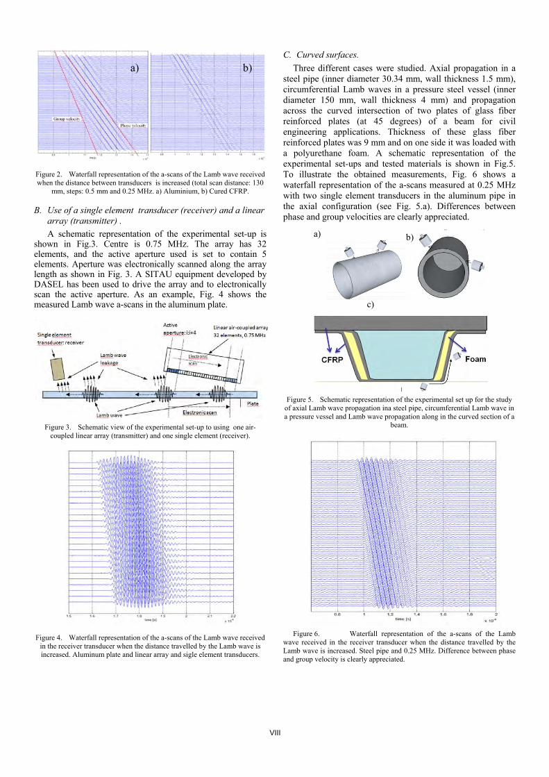
Figure 2. Waterfall representation of the a-scans of the Lamb wave received when the distance between transducers is increased (total scan distance: 130

mm, steps: 0.5 mm and 0.25 MHz. a) Aluminium, b) Cured CFRP.

B. Use of a single element transducer (receiver) and a lineararray (transmitter) .A schematic representation of the experimental set-up is

shown in Fig.3. Centre is 0.75 MHz. The array has 32 elements, and the active aperture used is set to contain 5 elements. Aperture was electronically scanned along the array length as shown in Fig. 3. A SITAU equipment developed by DASEL has been used to drive the array and to electronically scan the active aperture. As an example, Fig. 4 shows the measured Lamb wave a-scans in the aluminum plate.

Figure 3. Schematic view of the experimental set-up to using one air-coupled linear array (transmitter) and one single element (receiver).

Figure 4. Waterfall representation of the a-scans of the Lamb wave received in the receiver transducer when the distance travelled by the Lamb wave is increased. Aluminum plate and linear array and sigle element transducers.

C. Curved surfaces.Three different cases were studied. Axial propagation in a

steel pipe (inner diameter 30.34 mm, wall thickness 1.5 mm), circumferential Lamb waves in a pressure steel vessel (inner diameter 150 mm, wall thickness 4 mm) and propagation across the curved intersection of two plates of glass fiber reinforced plates (at 45 degrees) of a beam for civil engineering applications. Thickness of these glass fiber reinforced plates was 9 mm and on one side it was loaded with a polyurethane foam. A schematic representation of the experimental set-ups and tested materials is shown in Fig.5. To illustrate the obtained measurements, Fig. 6 shows a waterfall representation of the a-scans measured at 0.25 MHz with two single element transducers in the aluminum pipe in the axial configuration (see Fig. 5.a). Differences between phase and group velocities are clearly appreciated.

Figure 5. Schematic representation of the experimental set up for the study of axial Lamb wave propagation ina steel pipe, circumferential Lamb wave in a pressure vessel and Lamb wave propagation along in the curved section of a

beam.

Figure 6. Waterfall representation of the a-scans of the Lamb wave received in the receiver transducer when the distance travelled by the Lamb wave is increased. Steel pipe and 0.25 MHz. Difference between phase and group velocity is clearly appreciated.

a) b)

a) b)

c)

VIII

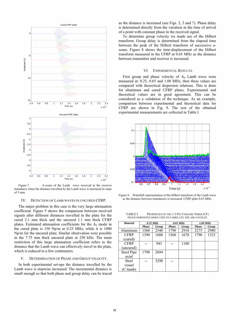
Figure 7. A-scans of the Lamb wave received in the receiver transducer when the distance travelled by the Lamb wave is increased in steps of 5 mm.

IV. DETECTION OF LAMB WAVES IN UNCURED CFRP.The major problem in this case is the very large attenuation

coefficient. Figure 5 shows the comparison between received signals after different distances travelled in the plate for the cured 2.1 mm thick and the uncured 1.1 mm thick CFRP plates. Estimated attenuation coefficients for the A0 mode in the cured plate is 150 Np/m at 0.25 MHz, while it is 1000 Np/m for the uncured plate. Similar observation were possible in the 7.75 mm thick uncured plate at 250 kHz. The main restriction of this large attenuation coefficient refers to the distance that the Lamb wave can effectively travel in the plate, which is reduced to a few centimeters.

V. DETERMINATION OF PHASE AND GROUP VELOCITY.In both experimental set-ups the distance travelled by the

Lamb wave is stepwise increased. The incremental distance is small enough so that both phase and group delay can be traced

as the distance is increased (see Figs. 2, 3 and 7). Phase delay is determined directly from the variation in the time of arrival of a point with constant phase in the received signal.

To determine group velocity we made use of the Hilbert transform. Group delay is determined from the elapsed time between the peak of the Hilbert transform of successive a-scans. Figure 8 shows the time-displacement of the Hilbert transform measured in the CFRP at 0.65 MHz as the distance between transmitter and receiver is increased.

VI. EXPERIMENTAL RESULTS.First group and phase velocity of A0 Lamb wave were

measured at: 0.25, 0.65 and 1.00 MHz, then these values are compared with theoretical dispersion relations. This is done for aluminum and cured CFRP plates. Experimental and theoretical values are in good agreement. This can be considered as a validation of the technique. As an example, comparison between experimental and theoretical data for CFRP are shown in Fig. 9. The rest of the obtained experimental measurements are collected in Table I.

Figure 8. Waterfall representation of the Hilbert transform of the Lamb wave as the distance between transducers is increased. CFRP plate 0.65 MHz.

TABLE I. PROPERTIES OF THE 1-3 PZT CERAMIC FIBER (CF) PIEZOCOMPOSITES DISKS USED TO FABRICATE THE AIR-COUPLED

Material 0.25 MHz 0.65 MHz 1.00 MHzPhase Group Phase Group Phase Group

Aluminum 1560 2540 1790 2910 2275 2980CFRP(cured)

1390 1600 1560 1678 1790 1323

CFRP(uncured)

-- 943 -- 1100

Steel Pipeaxial

1790 2694

Steel vessel

(C-lamb)

-- 3290 --

0.4 0.6 0.8 1 1.2 1.4 1.6 1.8 2 2.2 2.4

x 10-4

-15

-10

-5

0

Time (s)

Am

plitu

de (

V)

Cured FRP plate

0.4 0.6 0.8 1 1.2 1.4 1.6 1.8 2 2.2 2.4

x 10-4

-4

-3.5

-3

-2.5

-2

-1.5

-1

-0.5

0

0.5

1

Time (s)

Am

plitu

de (

V)

Uncured FRP plate

IX

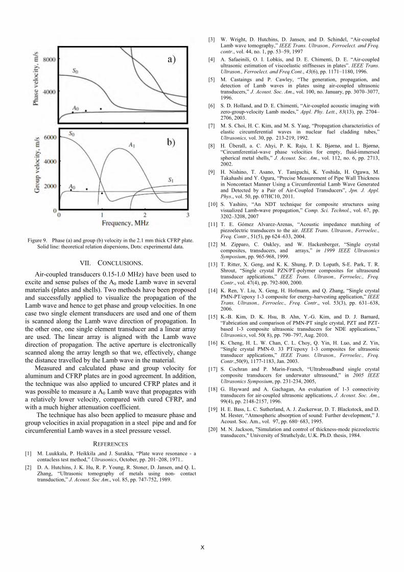
Figure 9. Phase (a) and group (b) velocity in the 2.1 mm thick CFRP plate. Solid line: theoretical relation dispersions, Dots: experimental data.

VII. CONCLUSIONS.Air-coupled transducers 0.15-1.0 MHz) have been used to

excite and sense pulses of the A0 mode Lamb wave in several materials (plates and shells). Two methods have been proposed and successfully applied to visualize the propagation of the Lamb wave and hence to get phase and group velocities. In one case two single element transducers are used and one of them is scanned along the Lamb wave direction of propagation. In the other one, one single element transducer and a linear array are used. The linear array is aligned with the Lamb wave direction of propagation. The active aperture is electronically scanned along the array length so that we, effectively, change the distance travelled by the Lamb wave in the material.

Measured and calculated phase and group velocity for aluminum and CFRP plates are in good agreement. In addition, the technique was also applied to uncured CFRP plates and it was possible to measure a A0 Lamb wave that propagates with a relatively lower velocity, compared with cured CFRP, and with a much higher attenuation coefficient.

The technique has also been applied to measure phase and group velocities in axial propagation in a steel pipe and and for circumferential Lamb waves in a steel pressure vessel.

REFERENCES [1] M. Luukkala, P. Heikkila ,and J. Surakka, “Plate wave resonance - a

contacless test method,” Ultrasonics, October, pp. 201–208, 1971..[2] D. A. Hutchins, J. K. Hu, R. P. Young, R. Stoner, D. Jansen, and Q. L.

Zhang, “Ultrasonic tomography of metals using non- contacttransduction,” J. Acoust. Soc Am., vol. 85, pp. 747-752, 1989.

[3] W. Wright, D. Hutchins, D. Jansen, and D. Schindel, “Air-coupledLamb wave tomography,” IEEE Trans. Ultrason., Ferroelect. and Freq.contr., vol. 44, no. 1, pp. 53–59, 1997

[4] A. Safaeinili, O. I. Lobkis, and D. E. Chimenti, D. E. “Air-coupledultrasonic estimation of viscoelastic stiffnesses in plates”. IEEE Trans.Ultrason., Ferroelect. and Freq.Cont., 43(6), pp. 1171–1180, 1996.

[5] M. Castaings and P. Cawley, “The generation, propagation, anddetection of Lamb waves in plates using air-coupled ultrasonictransducers,” J. Acoust. Soc. Am., vol. 100, no. January, pp. 3070–3077,1996.

[6] S. D. Holland, and D. E. Chimenti, “Air-coupled acoustic imaging withzero-group-velocity Lamb modes,” Appl. Phy. Lett., 83(13), pp. 2704–2706, 2003.

[7] M. S. Choi, H. C. Kim, and M. S. Yaag, “Propagation characteristics ofelastic circumferential waves in nuclear fuel cladding tubes,”Ultrasonics, vol. 30, pp. 213-219, 1992.

[8] H. Überall, a. C. Ahyi, P. K. Raju, I. K. Bjørnø, and L. Bjørnø,“Circumferential-wave phase velocities for empty, fluid-immersedspherical metal shells,” J. Acoust. Soc. Am., vol. 112, no. 6, pp. 2713,2002.

[9] H. Nishino, T. Asano, Y. Taniguchi, K. Yoshida, H. Ogawa, M.Takahashi and Y. Ogura, “Precise Measurement of Pipe Wall Thicknessin Noncontact Manner Using a Circumferential Lamb Wave Generatedand Detected by a Pair of Air-Coupled Transducers”, Jpn. J. Appl.Phys., vol. 50, pp. 07HC10, 2011.

[10] S. Yashiro, “An NDT technique for composite structures usingvisualized Lamb-wave propagation,” Comp. Sci. Technol., vol. 67, pp.3202–3208, 2007

[11] T. E. Gómez Alvarez-Arenas, “Acoustic impedance matching ofpiezoelectric transducers to the air. IEEE Trans. Ultrason., Ferroelec.,Freq. Contr., 51(5), pp 624–633, 2004.

[12] M. Zipparo, C. Oakley, and W. Hackenberger, “Single crystalcomposites, transducers, and arrays,” in 1999 IEEE UltrasonicsSymposium, pp. 965-968, 1999.

[13] T. Ritter, X. Geng, and K. K. Shung, P. D. Lopath, S-E. Park, T. R.Shrout, “Single crystal PZN/PT-polymer composites for ultrasoundtransducer applications,” IEEE Trans. Ultrason., Ferroelec., Freq.Contr., vol. 47(4), pp. 792-800, 2000.

[14] K. Ren, Y. Liu, X. Geng, H. Hofmann, and Q. Zhang, “Single crystalPMN-PT/epoxy 1-3 composite for energy-harvesting application,” IEEETrans. Ultrason., Ferroelec., Freq. Contr., vol. 53(3), pp. 631–638,2006.

[15] K.-B. Kim, D. K. Hsu, B. Ahn, Y.-G. Kim, and D. J. Barnard,“Fabrication and comparison of PMN-PT single crystal, PZT and PZT-based 1-3 composite ultrasonic transducers for NDE applications,”Ultrasonics, vol. 50( 8), pp. 790–797, Aug. 2010.

[16] K. Cheng, H. L. W. Chan, C. L. Choy, Q. Yin, H. Luo, and Z. Yin,“Single crystal PMN-0. 33 PT/epoxy 1-3 composites for ultrasonictransducer applications,” IEEE Trans. Ultrason., Ferroelec., Freq.Contr.,50(9), 1177-1183, Jan. 2003.

[17] S. Cochran and P. Marin-Franch, “Ultrabroadband single crystalcomposite transducers for underwater ultrasound,” in 2005 IEEEUltrasonics Symposium, pp. 231-234, 2005,

[18] G. Hayward and A. Gachagan, An evaluation of 1-3 connectivitytransducers for air-coupled ultrasonic applications, J. Acoust. Soc. Am.,99(4), pp. 2148-2157, 1996.

[19] H. E. Bass, L. C. Sutherland, A. J. Zuckerwar, D. T. Blackstock, and D.M. Hester, “Atmospheric absorption of sound: Further development,” J.Acoust. Soc. Am., vol. 97, pp. 680–683, 1995.

[20] M. N. Jackson, "Simulation and control of thickness-mode piezoelectrictransducers," University of Strathclyde, U.K. Ph.D. thesis, 1984.

X

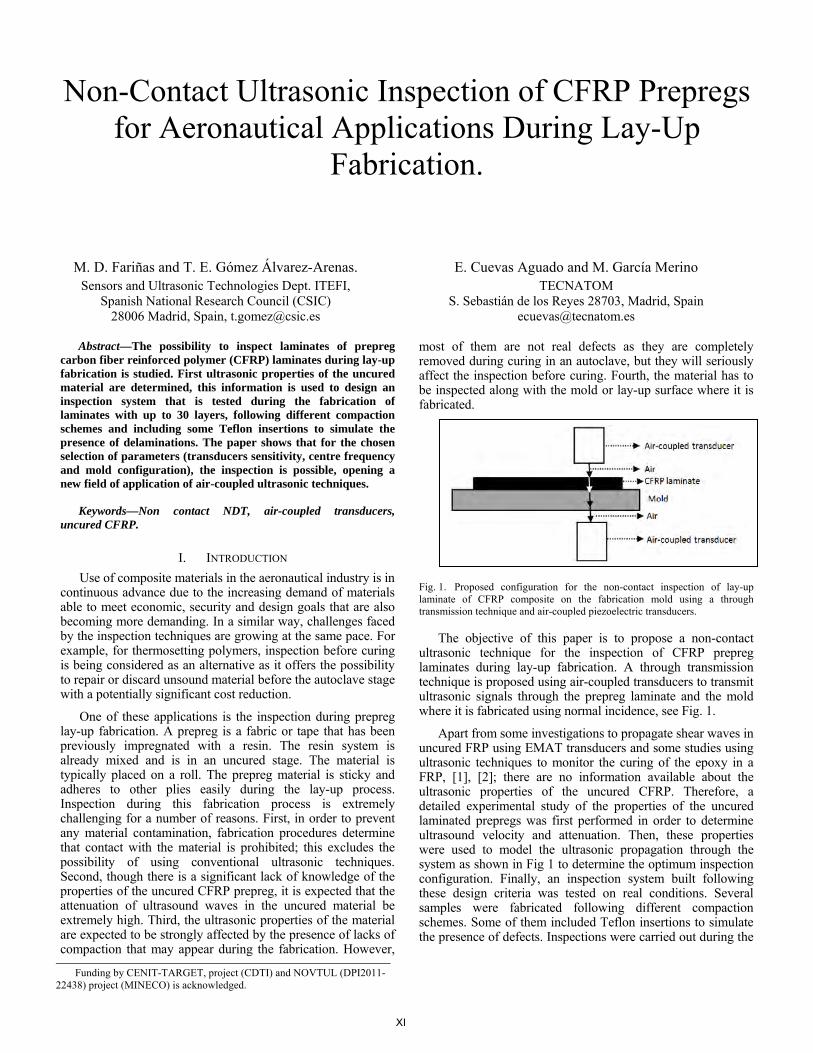
Non-Contact Ultrasonic Inspection of CFRP Prepregs for Aeronautical Applications During Lay-Up

Fabrication.

M. D. Fariñas and T. E. Gómez Álvarez-Arenas.Sensors and Ultrasonic Technologies Dept. ITEFI,

Spanish National Research Council (CSIC) 28006 Madrid, Spain, t.gomez@csic.es

E. Cuevas Aguado and M. García MerinoTECNATOM

S. Sebastián de los Reyes 28703, Madrid, Spainecuevas@tecnatom.es

Abstract—The possibility to inspect laminates of prepreg carbon fiber reinforced polymer (CFRP) laminates during lay-up fabrication is studied. First ultrasonic properties of the uncured material are determined, this information is used to design an inspection system that is tested during the fabrication of laminates with up to 30 layers, following different compaction schemes and including some Teflon insertions to simulate the presence of delaminations. The paper shows that for the chosen selection of parameters (transducers sensitivity, centre frequency and mold configuration), the inspection is possible, opening a new field of application of air-coupled ultrasonic techniques.

Keywords—Non contact NDT, air-coupled transducers, uncured CFRP.

I. INTRODUCTION

Use of composite materials in the aeronautical industry is in continuous advance due to the increasing demand of materials able to meet economic, security and design goals that are also becoming more demanding. In a similar way, challenges faced by the inspection techniques are growing at the same pace. For example, for thermosetting polymers, inspection before curing is being considered as an alternative as it offers the possibility to repair or discard unsound material before the autoclave stage with a potentially significant cost reduction.

One of these applications is the inspection during prepreg lay-up fabrication. A prepreg is a fabric or tape that has been previously impregnated with a resin. The resin system is already mixed and is in an uncured stage. The material is typically placed on a roll. The prepreg material is sticky and adheres to other plies easily during the lay-up process. Inspection during this fabrication process is extremely challenging for a number of reasons. First, in order to prevent any material contamination, fabrication procedures determine that contact with the material is prohibited; this excludes the possibility of using conventional ultrasonic techniques. Second, though there is a significant lack of knowledge of the properties of the uncured CFRP prepreg, it is expected that the attenuation of ultrasound waves in the uncured material be extremely high. Third, the ultrasonic properties of the material are expected to be strongly affected by the presence of lacks of compaction that may appear during the fabrication. However,

most of them are not real defects as they are completely removed during curing in an autoclave, but they will seriously affect the inspection before curing. Fourth, the material has to be inspected along with the mold or lay-up surface where it is fabricated.

Fig. 1. Proposed configuration for the non-contact inspection of lay-up laminate of CFRP composite on the fabrication mold using a through transmission technique and air-coupled piezoelectric transducers.

The objective of this paper is to propose a non-contact ultrasonic technique for the inspection of CFRP prepreg laminates during lay-up fabrication. A through transmission technique is proposed using air-coupled transducers to transmit ultrasonic signals through the prepreg laminate and the mold where it is fabricated using normal incidence, see Fig. 1.

Apart from some investigations to propagate shear waves in uncured FRP using EMAT transducers and some studies using ultrasonic techniques to monitor the curing of the epoxy in a FRP, [1], [2]; there are no information available about the ultrasonic properties of the uncured CFRP. Therefore, a detailed experimental study of the properties of the uncured laminated prepregs was first performed in order to determine ultrasound velocity and attenuation. Then, these properties were used to model the ultrasonic propagation through the system as shown in Fig 1 to determine the optimum inspection configuration. Finally, an inspection system built following these design criteria was tested on real conditions. Several samples were fabricated following different compaction schemes. Some of them included Teflon insertions to simulate the presence of defects. Inspections were carried out during the

Funding by CENIT-TARGET, project (CDTI) and NOVTUL (DPI2011-22438) project (MINECO) is acknowledged.

XI

fabrication to test the influence of both the number of layers and the compaction processes.

II. ULTRASONIC PROPERTIES OF UNCURED LAMINATES.A 1 mm thick uncured CFRP laminate were used for the

characterization of the material. For comparison purposes a 2 mm thick cured CFRP laminate were also characterized. Towards this end, the technique described in [3] was used. This consists on measuring the magnitude and phase spectra of the transmission coefficient around the first order thickness resonance using a through transmission technique and air-coupled wide-band transducers [4], [5] and then solving the inverse problem.

The plates were measured in ten different points to determine the spatial variability. Two representative measurements are shown in Fig. 2. Averaged obtained parameters and standard deviation are collected in Table I. The more remarkable difference between both materials is the attenuation coefficient that is much larger in the uncured laminate, seriously limiting the inspection possibilities. The other differences are a slightly lower density in the uncured CFRP, a significantly lower velocity, due to the comparatively lower velocity in the uncured resin, and a larger variability of the measured properties. Acoustic impedance of the uncured CFRP laminate is lower (2.16 MRayl) compared with the cured material (5.27 MRayl).

TABLE I. PROPERTIES OF CURED AND UNCURED CFRP LAMINATES

Material Density (kg/m3)

Ultrasound velocity (m/s)

Ultrasound attenuation @ fres (Np/m)

Uncured 1580 ± 120 1370 ± 175 540 ± 80

Cured 1850 ± 120 2840 ± 40 20 ± 2

Fig. 2. Measured and calculated magnitude and phase spectra of the transmission coefficient for two FRPC plates, cured (2mm thick) and uncured (1 mm thick).

III. DETERMINATION OF THE INSPECTION POSIBILIITIESUSING AIR-COUPLED ULTRASOUNDS: DESIGN PARAMETERS

FOR THE INSPECTION SYSTEM. As the material must be inspected along with the mold

where it is fabricated, the design variables of the inspection system to be considered are: 1) Mould material and thickness, and 2) Transducers centre frequency and bandwidth. A theoretical simulation of the ultrasound transmission is performed using the material parameters previously obtained and varying these design variables to find out the best configuration. A 1D problem was considered: plane waves and normal incidence, and a linear variation of the attenuation with the frequency. It is assumed a thickness of the CFRP laminate of 7 mm in all cases. Following our previous experience, the maximum acceptable through transmission losses is set to 100 dB, i.e. beyond that value it is considered that the inspection is not possible with the available technology.

As the mold has to be made of a metal, the selected option was aluminum because of its relatively lower acoustic impedance, and cost. Fig. 3 shows the calculated Insertion loss (IL) vs. frequency for three different mold thicknesses: 2, 6 and 13 mm. The first conclusion is that working frequency must be limited below 0.55 MHz, the second one is that a significant increase of the transmitted signal amplitude can be achieved if the working frequency is tuned to the thickness resonance of the mold. So, with the 6 mm thick mold the thickness resonance appears at 0.52 MHz, minimum IL= -92 dB, for the 13 mm thick mold, the thickness resonance appears at 0.25 MHz with a minimum IL of -78 dB. Therefore, the proposed configuration consists on a 13 mm thick mold and a pair of 0.25 MHz air-coupled transducers.

Fig. 3. Calculated spectra of the Insertion loss of the FRCP laminate and the aluminum mold for three different mold thicknesses (a: 2 mm; b: 6 mm; c: 13 mm). Green line indicated the location of the 0.25 MHz frequency and the red line indicates the maximum inspection frequency for the -100 dB limit. 3. d: simulated transmitted pulse for the 13 mm mold using a pair of 0.25 MHz air-coupled transducers.

-80

-70

-60

-50

-40

Mag

nitu

de (d

B) cured

uncured

0.30 0.45 0.60 0.75 0.90

5

10

15

20

25

30

Phas

e (ra

d)

Frequency (MHz)

cured

uncured

Transmission coefficient spectra

a b

c d

XII

IV. ULTRASONIC INSPECTION SYSTEM.

A. Transducers.The impulse response and sensitivity obtained with the pair

of transducers used for this work, operated in through transmission, separated 2 cm in air, using a Panametrics Pulser/Receiver (PR 5058), with spike amplitude set to 200 V and receiver gain set to 0 dB, and a Tektronix Oscilloscope DPO7054 is shown in Fig. 4. Sensitivity is calculated as the ratio of the FFT of the electric voltage measured on the receiver terminals to the one measured on the transmitter terminals. Peak sensitivity is -24.6 dB, this figure is the key to set the limit of the maximum acceptable insertion losses for a through transmission test at -100 dB.

0 30 60 90 120 150 180-0,8

-0,6

-0,4

-0,2

0,0

0,2

0,4

0,6

0,8

Ampl

itude

(V)

Time (µs)

0.15 0.20 0.25 0.30 0.35 0.40-90

-80

-70

-60

-50

-40

-30

-20

Sens

itivity

(dB)

Frequency (MHz)

Peak: -24.6 dB @ 240 kHzUseful badwidth: 62%Centre frequency: 240 kHz

Fig. 4. Measured impulse response and sensitivity of the 0.25 MHz air-coupled transducers employed for the tests.

B. Electronics.Two different pulser/receiver systems were successfully

used. A Panametrics P/R 5058, and a DASEL USB-ultrascope that provide a tone burst (square wave, we used between 1 and 5 cycles) up to 400 V and 60 dB gain in reception.

C. Mechanics.The transducers were mounted on a U shaped holder as

shown in Fig. 5. The holder was fitted into an automatic and portable scanning system, developed by Tecnatom, to perform both punctual through transmission measurements and C-Scans. This system can be put in place to perform the tests and then taken away to allow for the space for the machine that puts the layers of prepreg CFRP.

D. Materials and inspection scheme.Several samples (300 x 300 mm and up to 30 layers) of

CFRP, equal to others used in the aeronautical industry, were

fabricated at FIDAMC (Getafe, Spain) following different compaction scheme. Some samples were fabricated without compacting them, and some other were compacted at different stages. The compactions were performed using conventional vacuum bags. Two different compaction times were used: short (15-30 min) and large (from 4 to 8 hours). In addition, some of them included 10 x 10 mm Teflon insertions at three different depths (2, 15 and 28 layers) to simulate the presence of local defects (delaminations).

Fig. 5. Picture of the aluminum mold with the CFRP, the transducers and the scanning system.

V. RESULTS.

A. Transmission of airborne ultrasonic signals through theCFRP laminate and aluminum mold system.Fig 6. shows the transmitted signal from Tx to Rx for

several cases. The transmitted signal through the CFRP-mold system is clearly identified and the SNR figure is pretty good (>30 dB). Reverberations in the airgaps between transducers and sample are clearly appreciated revealing the importance of using wideband transducers.

Fig. 6. Transmitted signal from Tx-transducer to Rx-transducer for three cases: Up: no sample between Tx and Rx. Middle: CFRP laminate (8 layers) and 13 mm aluminum mold. Bottom: CFRP laminate (30 layers) and 13 mm aluminum mold.

-2-1012

No sample

-0,2-0,10,00,10,2

Ampl

itude

(V) 8 layers, long compaction

50 100 150 200 250 300 350-0,2-0,10,00,10,2 30 layers, long compaction

Time (µs)

XIII

For the inspection of the 8 layers laminate the pulse amplitude of the Panametrics 5058 were set to 400 V and the gain in reception to 40 dB. For the 30 layers laminate, the configuration was 400V and 50 dB, respectively.

The measurement of the variation in the time of flight as the number of layed layers increased permitted to us to determine the ultrasound velocity , which turned out to be slightly smallerthan the values obtained in the preeliminary study, about 950 m/s.

B. Influence of compaction.To determine the influence of the compaction degree on the

inspection possibilities several laminates were fabricated (up to 30 layers) following different compaction schemes. In all these cases layers were put manually, which is the worst possible scenario because in this case, the degree of compaction is comparatively smaller compared with the case when layers are put by a machine. Comparing the amplitude of the signal received with different number of layers after the same compaction procedure it was possible to estimate the attenuation coefficient in the laminate which results to be extremely dependent on the degree of compaction. Results are summarized in Table II. These, along with the estimation of the level of noise permit to determine the maximum number of layers that can be inspected with this configuration. For example, after a short compaction, the results suggests that the inspection limit is about 12 layers, for non compacted material, the limit is reduced to about 3 layers, while after a long compaction it would be possible to inspect up to 90 layers.

TABLE II. AVERAGED VALUE OF THE MEASURED ATTENUATION PER LAYER FOR DIFFERENT TYPES OF COMPACTIONS FOR ALL THE TESTED CASES.

Compaction Attenuation (dB/layer) @ 0.25 MHz

Long 0.3-0.75

Short 2.5-3.0

None 7-10

Fig. 7. Linear scan along two Teflon insertions, laminate with 24 layers measured after a long compaction.

C. Detection of Teflon insertions.Fig. 7 shows the result of a liner scan over two 10 x 10 mm

Teflon insertions located at a distance of 75 and 150 mm, respectively, from the scan origin. The drop of signal amplitude due to the presence of the insertions is between 7 and 12 dB and the actual size of the insertion is consistent with the size of the amplitude drop.

VI. CONCLUSIONS.This paper studies the possibility to use an air-coupled and

through transmission ultrasonic technique to inspect prepreg CFRP laminates during lay-up fabrication (i.e. before the resin cures). The main challenges of this application are the impossibility to touch the material during the inspection, the large attenuation coefficient in the uncured CFRP laminate and the need to perform the inspection together with the fabrication mold. An air-coupled and through transmission technique is proposed. To minimize the effect of the very large insertion loss, a pair of wide band and low frequency (0.15-0.35 MHz), high sensitivity (-24 dB) transducers with active area diameter of 25 mm were employed together with a conventional pulser/receiver. In addition, a mold of aluminum, 13 mm thick, was proposed, so the mold presented a thickness resonance within the transducers bandwidth so transmission of energy is enhanced. With this configuration it was possible to inspect well compacted laminates with up to 30 layers, and the estimation is that the maximum thickness that can be inspected is about 90 layers. It was also possible to detect the presence of Teflon (10 x 10 mm) insertions at different depths, with an amplitude loss about 7-12 dB compared with insertion-free areas. Finally, the paper reveals that one of the key factors to determine the possibility to inspect prepreg lay-up CFRP laminates is the ultrasound attenuation. This attenuation is largely determined by the degree of compaction of the laminate; it can be more than one order of magnitude larger in the case of poorly compacted laminates compared with well compacted ones.

REFERENCES [1] D. K. Hsu, Kwan-Hee Im, and In-Young Yang, “Applications of

Electromagnetic Acoustic Transducers in the NDE of Non-Conducting Composite Materials,” KSME International Journal, vol. 13, no. 5, pp.403–413, 1999.

[2] D. DeVries, “Design of a Cure Monitoring System for CompositeAircraft Repair Patches,” MsSc Department of Aerospace EngineeringUniversity of Toronto, 1996

[3] T. E. Gómez Alvarez-Arenas, “Simultaneous determination of theultrasound velocity and the thickness of solid plates from the analysis ofthickness resonances using air-coupled ultrasound,” Ultrasonics, vol.50(2), pp. 104–109, 2010.

[4] T. E. Gómez Alvarez-Arenas, “Acoustic impedance matching ofpiezoelectric transducers to the air,” IEEE transactions on ultrasonics,ferroelectrics, and frequency control, 51(5), pp. 624–33, 2004.

[5] T. E. Gómez Alvarez-Arenas, “Air-coupled piezoelectric transducerswith active polypropylene foam matching layers.,” Sensors, vol. 13, no.5, pp. 5996–6013, 2013.

XIV

Modification of the Ultrasonic Properties of Elastomers Loaded with Magnetic Particles by

Applying Magnetic Fields During Curing.

I. Agirre Olabide, M. J. Elejabarrieta and M. M. Bou-Ali

Mechanical and Manufacturing Department Mondragon Goi Eskola Politeknikoa

Mondragon, Spain Iker.agirreo@alumni.mondragon.edu

M. D. Fariñas and T. E. Gómez Alvarez-ArenasSensors and Ultrasonic Technologies Dept. ITEFI,

Spanish National Research Council (CSIC) 28006 Madrid, Spain,

t.gomez@csic.es

Abstract— Particle loaded polymers and elastomers have been largely used in different ultrasonic applications like backing materials and matching layers because composite properties (velocity, attenuation, density and impedance) can be easily engineered by changing the filler concentration. Recently, the use of magnetic particles has been theoretically proposed as a means to produce active matching layers whose response can be modified upon the application of magnetic fields. In this paper, we propose to introduce modifications of the composite properties by using magnetic particles and applying magnetic fields during curing to establish well defined patterns in the spatial distribution of the particles within the elastomer that induce material anisotropy that effectively modify ultrasonic properties.

Keywords— Magnetorheological elastomers, ultrasonic properties, isotropic and anisotropic, smart magnetic materials.

I. INTRODUCTION

Magnetorheological elastomers (MRE) are considered smart materials due to the possibility to modify their properties when an external magnetic field is applied. Basically, MRE consist on magnetic particles embedded in a polymeric matrix, where many different polymeric matrices can be used: natural rubbers, silicone rubbers, etc [1-2], with the unique requirement that the matrix has to be paramagnetic. In the ultrasonic field, 0-3 connectivity composite materials have been used as backing and matching layers materials.. More recently, 0-3 connectivity composites made with magnetic particles have been proposed either to change the magnetic properties of the composite [3] or to produce active matching layers whose properties can be changed upon the application of a magnetic field [4].

The most common magnetic material used for the synthesis of MRE are iron micro-particles, which size is between 1 µm and 10 µm [5-6]. However, larger particles until 200 µm and irregular shape particles have also been used [7].

These particles can be randomly distributed within the polymeric matrix or aligned in chains. The alignment of the particles is obtained by the application of an external magnetic

field during the so-called pre-structure process [6], due to the interaction between the particles; these samples are called anisotropic MRE to differentiate them from samples produced without any magnetic field where the particles present a random and globally isotropic distribution [7-8].

The aim of this work is to determine and analyze the influence of the particle concentration and the pre-structure process on the ultrasonic properties of the MRE as a first step towards achieving materials whose properties can be either engineered during fabrication or altered after fabrication…

II. SYNTHESIS

The matrix used in this work was a two components silicone rubber. The silicone WACKER Elastosil® M 4644 A and the vulcanizer WACKER Elastosil® M 4644 B, both are mixed in the ratio10:1 respectively.

Carbonyl iron powder particles (average particle size of 1.25±0.55 μm) and spherical shape, supplied by BASF (Germany) were used to make the samples. The samples were produced by mixing the silicone rubber A component and the particles and subjecting the mixture to vacuum cycles to extract the air bubbles generated during the mixing process. Subsequently, the vulcanizer was added and mixed; then, vacuum cycles were applied at the same conditions. The cycle quantity varies with the particle concentration. Once a homogeneous mixture is obtained two different pre-structure conditions were applied to obtain isotropic or anisotropic MRE samples, respectively: under an external magnetic field and without its influence. The thickness of the samples is of 1 mm in all cases.

Anisotropic samples have been pre-structured by a device where neodymium magnets are applied (Fig. 1). Thanks to the ferromagnetic plates, the device guaranties a homogeneous magnetic field. That magnetic field is applied in the thickness direction of the sample [7]. The intensity of the field during the pre-structure is 0.13±0.01T and is measured by a Gaussmeter FH-54.

The present study has been partially supported by ACTIMAT and MAGNETOBUSH (UE2013-09) projects, Research Group program (IT557-10) from the Basque government, and by the MAGNETO (INNPACTO-020000-2010-006), AVISUINT (DPI 2012-36366) and NOVTUL (DPI2011-22438) from the Spanish government.

XV

Fig. 1. Sketch of the anisotropic pre-structure device.

Samples with seven different values particle volume concentration were synthesized, 0%, 5%, 10%, 15%, 20%, 25% and 30%, respectively. The maximum concentration is defined by the CPVC [5]. As explained before, two pre-structure conditions were used to obtain either isotropic or anisotropic samples.

III. ULTRASONIC CHARACTERIZATION

Several ultrasonic techniques have been tested to determine the ultrasonic properties of these materials: ultrasonic velocity and attenuation and the variation in these parameters with the frequency. In all cases a through transmission technique was employed, but different coupling methods were tried: water immersion, direct contact and gel coupling and air-coupling. Obtained results were similar, but the air-coupled technique is preferred because it offers a better possibility to study changes in materials properties upon the application of a magnetic field; it is also more convenient to measure shear waves and hence to get shear elastic modulus and Poisson’s ratio which will be the next steps of this investigation.

The technique is described in [8]. The magnitude and the phase spectra of the transmission coefficient of a plate-shaped sample are measured at normal incidence and in a frequency band were, at least, one order of thickness resonances of the sample is observed. Effective properties of the material are obtained by solving the inverse problem.

The measurements were performed using a pair of air-coupled wide-band transducers fabricated at US-Biomat research group (ITEFI, CSIC) [9], [10]. Transducers were embedded in a U-shaped holder that keeps them aligned and also provides a slot for the correct placement of the sample (see Fig. 2). Transmitter transducer were driven by a 200 V amplitude semicycle of square wave, provided by a conventional pulser (Panametrics 4077), the received signal was analogically amplified (30 dB), with the reception function of the Panametrics 5077 and then digitized by a Tektronix scope (TDS5052). The transmitted signal from transmitter to receiver without any sample between them is shown in Fig. 3 (up). Fig. 3 (down) shows the sensitivity vs frequency calculated as the ratio of the amplitude of the FFT of the electrical signal measured at receiver terminals to the amplitude of the FFT of the electrical signal measured at the transmitter terminals.

Fig. 2. Picture of the transmitter-receiver pair of transducers embedded in the U-shaped holder for air-coupled through transmission measurements. The slotbetween trnasmitter and receiver is used to place the samples.

0 10 20 30 40 50 60

-0.9

-0.6

-0.3

0.0

0.3

0.6

0.9

Am

plit

ude (

V)

Time (s)

0.4 0.8 1.2 1.6 2.0-90

-60

-30

Se

nsitiv

ity (

dB

)

Frequency (MHz)

Fig. 3. Up: transmitted signal from transmitter to receiver in the time domain without any sample between them. Down: sensitivity vs frequency

IV. RESULTS

Below are shown the results obtained by the air-coupling technique in the range of 0.34 and 0.95 MHz. First of all, the temporal signal measured by the transducers is analyzed and the quality factor (Q factor) is obtained. Towards this end, the decline of the temporal signal has been adjusted by an exponential function. Finally, the results obtained by the analyzing the amplitude spectrum are shown: longitudinal velocity and the quality factor.

Fig. 4 shows the temporal signal measured by the transducers. But the data used at the present work corresponds to the rectangular window indicated at the figure. The temporal signal corresponds to a single harmonic oscillation under damped system.

XVI

0 1 2 3 4

x 10-4

-0.03

-0.02

-0.01

0

0.01

0.02

0.03

Time [s]

Am

plit

ude [V

]

Fig. 4. Temporal signal of the sample without particles.

From the temporal signal the oscillation period, T is defined (Fig. 3). The maximum points of each oscillation are approximated by the least squares method to (1), where the amplitude (A0) and the quality factor (Q) are defined.

t

QA

21-

0 e

where t is the time and ω is the fundamental natural frequency of the system. That frequency is obtained by (2) and the period (T), for the case of a week damping.

Tπ2

0 0.5 1 1.5

x 10-4

-0.01

-0.005

0

0.005

0.01

Time [s]

Am

plit

ude [V

]

Temporal signal

Exponent

T

Fig. 5. Temporal signal and the approximation by a exponential function.

The results obtained from the analysis are shown in Fig. 5. The factor decreases with the increment of the particle concentration, which means that the temporal signal attenuation increases with the concentration. Besides, the

anisotropic samples has a higher attenuation than the isotropic ones, in other words, the alignment of the particles increases the damping.

0 5 10 15 20 25 3020

30

40

50

60

70

80

90

Volumetric concentration [%]

Q facto

r

Isotropic

Anisotropic

Fig. 6. Quality factor obtained by the temporal signal in function fo the volumteric concentration.

After the analysis of the temporal signal, the Fourier transform has been obtained, and an approximation has been made to obtain different parameters (Fig. 6).

3 4 5 6 7 8 9 10 11

x 105

-70

-65

-60

-55

-50

-45

-40

-35

-30

-25

Frequency [Hz]

Am

plit

ude

Measurement

Approach

Fig. 7. Spectrum modulus, experimental and the approach.

From the spectrum approach longitudinal velocity is obtained (Fig. 7). Whereas, the velocity decreases with particle concentration, the influence of the pre-structure cannot be observed. This means that the ultrasonic wave has more difficulties with a higher particle concentration.

0 5 10 15 20 25 30650

700

750

800

850

900

950

1000

1050

Volumetric concentration [%]

Lo

ng

itu

din

al ve

locity [m

/s]

Isotropic

Anisotropic

Fig. 8. Longitudinal velocity from the spectrum approach in function of the particle volume fraction.

The quality factor also is obtained from the spectrum approach (Fig. 7). The factor decreases with the increment of the particle concentration and the damping is larger for anisotropic samples.

Those trends are observed using two different techniques, but there is a difference in the value. This is because at the spectrum analysis a calibration is used to eliminate the band effect of the transducers.

0 5 10 15 20 25 3015

20

25

30

35

40

45

50

Volumetric concentration [%]

Q facto

r

Isotropic

Anisotropic

Fig. 9. Quality factor obatained from the spectrum approach at the resonance frequency in function of the volumetric concentration.

V. CONCLUSIONS

The increase of the particle concentration from 0 to 30% reduces the longitudinal velocity from 1000 to 700 m/s. This effect is the combined result of the density increase of the composite when the particle concentration increases plus the reduced influence of the particles on the overall elasticity of the composite. This behavior follows the theoretical predictions of Hashin and Shtrikman [11] and the measurements performed before in polymer loaded with non magnetic particles [12] and [13]. However, no effect of the pre-structure obtained with a

magnetic field has been observed on the ultrasonic velocity of the longitudinal wave in this frequency range. On the other hand, the quality factor also increases when the particle concentration increases, which means that the attenuation is higher. This larger attenuation is the result of the scattering losses introduced by the particles; In this case, the quality factor depends on the pre-structure process: the anisotropic samples present a higher attenuation than the isotropic samples. Further investigations will focus on the study of the propagation of longitudinal waves in the plate direction and shear waves in the direction normal to the plate. In this case, it is expected that both velocity and attenuation will present different values depending on the direction of the polarization compared with the direction of particle alignment.

REFERENCES [1] L. Chen, X. Gong, W. Jiang, J. Yao, H. Deng and W. Li,

"Investigation on magnetorheological elastomers based on natural rubber," J.Mater Sci., vol. 42, pp. 5483-5489, 2007.

[2] M. Kallio, "The elastic and damping properties of magnetorheological elastomers," VTT Publ., 2005.

[3] M. Teirikangas, “Advanced 0–3 ceramic polymer composites for high frequency applications.” PhD Thesis, Dept. of Electrical Engineering, University of Oulu. 2011

[4] A. J. Mulholland, R. L. O’Leary, N. Ramadas, A. Parr, A. Troge, R. Pethrick, and G. Hayward, “A theoretical analysis of a piezoelectricultrasound device with an active matching layer,” Ultrasonics, vol.47(1-4), pp. 102–110, 2007.

[5] A. Boczkowska, S. F. Awietjan, T. Wejrzanowski, and K. J. Kurzydowski, "Image analysis of the microstructure of magnetorheological elastomers," J. Mater. Sci., vol. 44, pp. 3135-3140, 2009.

[6] J. Li, X. Gong, Z. Xu, and W. Jiang, "The effect of pre-structure process on magnetorheological elastomer performance," International Journal of Materials Research, vol. 99, pp. 1358-64, 12, 2008.

[7] M. Lokander, and B. Stenberg, "Performance of isotropic magnetorheological rubber materials," Polym. Test., vol. 22, pp. 245-51, 2003.

[8] Z. Varga, G. Filipcsei, and M. Zrinyi, "Magnetic field sensitive functional elastomers with tuneable elastic modulus," Polymer, vol.47, pp. 227-233, 2006.

[9] T. E. Gómez Alvarez-Arenas, “Simultaneous determination of the ultrasound velocity and the thickness of solid plates from the analysisof thickness resonances using air-coupled ultrasound,” Ultrasonics, vol. 50(2), pp. 104–109, 2010.

[10] T. E. Gómez Alvarez-Arenas, “Acoustic impedance matching of piezoelectric transducers to the air,” IEEE transactions on ultrasonics, ferroelectrics, and frequency control, 51(5), pp. 624–33, 2004.

[11] T. E. Gómez Álvarez-Arenas, T. R. Shrout, S. J. Zhang and H. J. Lee,“Air-Coupled Transducers Based on 1-3 Connectivity Single CrystalPiezocomposites,” 2012 IEEE International Ultrasonics Symposium Proceedings, pp. 2230-2233, 2012.

[12] Z. Hashin, S. Shtrikman, “A variational approach to elastic behaviour of multiphase materials,” J. Mech. Phys. Solids, vol. 11, pp. 127, 1963.

[13] T. E. Gómez Alvarez-Arenas, A. Mulholland, G. Hayward, J.Gomatam, “Wave propagation in 0-3/3-3 connectivity compositeswith complex microstructure,” Ultrasonics, 38(9), pp. 897–907. 2000. T. Nguyen, M. Lethiecq, F. Levassort, L. Pourcelot, “Experimental verification of the theory of elastic properties usisng scattering approximations in (0-3) connectivity composite materials,” IEEETrans. Ultrason. Ferroelec., Freq., Contrl. Vol 43(4), pp. 640-645, 1996.

XVII