ESSAYS ON MEXICAN MIGRATION

by

Heriberto Gonzalez Lozano

B.A., Universidad Autonóma de Nuevo León, 2005

M.A., University of Pittsburgh, 2011

Submitted to the Graduate Faculty of

the Dietrich School of Arts and Sciences in partial ful�llment

of the requirements for the degree of

Doctor of Philosophy

University of Pittsburgh

2013

UNIVERSITY OF PITTSBURGH

DIETRICH SCHOOL OF ARTS AND SCIENCES

This dissertation was presented

by

Heriberto Gonzalez Lozano

It was defended on

August 26th, 2013

and approved by

Randall Walsh, Department of Economics, University of Pittsburgh

Daniel Berkowitz, Department of Economics, University of Pittsburgh

Daniele Coen-Pirani, Department of Economics, University of Pittsburgh

Marie Connolly, Department of Economics, Chatham University

Dissertation Director: Randall Walsh, Department of Economics, University of Pittsburgh

ii

ESSAYS ON MEXICAN MIGRATION

Heriberto Gonzalez Lozano, PhD

University of Pittsburgh, 2013

In this dissertation I study di¤erent aspects of the Mexican migration to the United States.

First, I introduce one of the most complete sources of information of Mexican migrants in the

United States, the Survey of Migration to the Northern Border. Then I study the selectivity

of Mexican migration. I test Borjas�1987 negative selection hypothesis which states that

individuals migrating from states with more unequal income distribution and higher returns

to education will be more negatively selected. I analyze the degree of selectivity of immigrants

by exploiting the variation in returns to education and income inequality across Mexican

states over time. I use Borjas�selection model to infer worker�s unobservable skills. The

results support Borjas�hypothesis, there is evidence of negative selection in terms of years

of schooling and unobservable skills. Moreover, I predict the wages in the United States of

recently arrived migrants and �nd that higher income inequality is associated with lower

observable skills.

One channel through which migration may reduce poverty is by enhancing the asset

positions and productivity levels of poor households, either via remittances, savings, and

human capital accumulation. In this dissertation I assess the impact of return migration

on self-employment exploiting the variation in return migration rates to di¤erent states

of Mexico. I predict return migration to di¤erent Mexican states by using past migration

patterns and use these predicted rates as instruments for return migration avoiding potential

endogeneity issues. The results show that return migration exerted a positive but small

impact on the probability of self-employment in Mexico between 1999 and 2010.

In recent years, Mexico has experienced a dramatic surge in homicides driven by the

iii

violent struggle between and within criminal organizations to control the drug trade business.

In the last chapter I study the e¤ect of drug-violence on the out�ows of migrants from

Mexico to the United States. The results show that individuals from Western and Southern

Mexico are more likely to change their migratory behavior in response to changes in violence.

Violence increases migration rates from Western Mexico but decreases migration rates from

Southern Mexico.

iv

TABLE OF CONTENTS

PREFACE . . . . . . . . . . . . . . . . . . . . . . . . . . . . . . . . . . . . . . . . . xii

1.0 INTRODUCTION . . . . . . . . . . . . . . . . . . . . . . . . . . . . . . . . . 1

2.0 SURVEY OF MIGRATION TO THE NORTHERN BORDER (EMIF) 4

2.1 Introduction . . . . . . . . . . . . . . . . . . . . . . . . . . . . . . . . . . . 4

2.2 Migrants returned by the Border Patrol . . . . . . . . . . . . . . . . . . . . 6

2.2.1 Description, advantages and disadvantages of using this sample . . . . 6

2.3 Northward-bound migrants with destinations in either Mexican border cities

or the US . . . . . . . . . . . . . . . . . . . . . . . . . . . . . . . . . . . . . 6

2.3.1 Description, advantages and disadvantages of using this sample . . . . 6

2.4 Southward-bound migrants returning to Mexico from the United States . . . 12

2.4.1 Description, advantages and disadvantages of using this sample . . . . 12

2.4.2 Return Migration: EMIF and Mexican census data . . . . . . . . . . . 17

2.4.3 Survey of Migration to the Northern Border (EMIF) and Current Pop-

ulation Survey (CPS) . . . . . . . . . . . . . . . . . . . . . . . . . . . 18

3.0 TESTINGBORJAS�NEGATIVE SELECTIONHYPOTHESIS AMONG

MEXICAN IMMIGRANTS IN THE UNITED STATES . . . . . . . . . 22

3.1 Motivation . . . . . . . . . . . . . . . . . . . . . . . . . . . . . . . . . . . . 22

3.2 Literature Review . . . . . . . . . . . . . . . . . . . . . . . . . . . . . . . . 24

3.3 Data . . . . . . . . . . . . . . . . . . . . . . . . . . . . . . . . . . . . . . . . 26

3.4 Selectivity in terms of Observable Skills . . . . . . . . . . . . . . . . . . . . 31

3.4.1 Model . . . . . . . . . . . . . . . . . . . . . . . . . . . . . . . . . . . . 31

3.4.2 Estimating Returns to Education . . . . . . . . . . . . . . . . . . . . 32

v

3.4.3 Years of Schooling of Mexican immigrants over time . . . . . . . . . . 33

3.4.4 Selectivity of Migrants from Di¤erent Mexican States . . . . . . . . . 36

3.4.4.1 Empirical Speci�cation . . . . . . . . . . . . . . . . . . . . . . 36

3.4.4.2 Results . . . . . . . . . . . . . . . . . . . . . . . . . . . . . . . 37

3.5 Selectivity in terms of Unobservable Skills . . . . . . . . . . . . . . . . . . . 39

3.5.1 Borjas�Model . . . . . . . . . . . . . . . . . . . . . . . . . . . . . . . 39

3.5.2 Selectivity of Legal and Illegal Workers . . . . . . . . . . . . . . . . . 40

3.5.3 Empirical Speci�cation . . . . . . . . . . . . . . . . . . . . . . . . . . 43

3.5.4 Results . . . . . . . . . . . . . . . . . . . . . . . . . . . . . . . . . . . 48

3.6 Conclusions . . . . . . . . . . . . . . . . . . . . . . . . . . . . . . . . . . . . 53

4.0 RETURN MIGRATION AND SELF-EMPLOYMENT IN MEXICO . 55

4.1 Motivation . . . . . . . . . . . . . . . . . . . . . . . . . . . . . . . . . . . . 55

4.2 Literature Review . . . . . . . . . . . . . . . . . . . . . . . . . . . . . . . . 57

4.3 Data . . . . . . . . . . . . . . . . . . . . . . . . . . . . . . . . . . . . . . . . 60

4.4 Self-employment and Return Migration in Mexico . . . . . . . . . . . . . . . 64

4.5 Empirical Speci�cation . . . . . . . . . . . . . . . . . . . . . . . . . . . . . . 66

4.6 Results . . . . . . . . . . . . . . . . . . . . . . . . . . . . . . . . . . . . . . 68

4.7 Conclusions . . . . . . . . . . . . . . . . . . . . . . . . . . . . . . . . . . . . 72

5.0 DRUG VIOLENCE AND MIGRATION FLOWS . . . . . . . . . . . . . 74

5.1 Motivation . . . . . . . . . . . . . . . . . . . . . . . . . . . . . . . . . . . . 74

5.2 Literature Review . . . . . . . . . . . . . . . . . . . . . . . . . . . . . . . . 76

5.3 Data . . . . . . . . . . . . . . . . . . . . . . . . . . . . . . . . . . . . . . . . 77

5.4 Empirical Speci�cation . . . . . . . . . . . . . . . . . . . . . . . . . . . . . . 81

5.4.1 E¤ect of Violence on the Out�ows of Migrants: Sample of Migrants

who Intend to Enter the US . . . . . . . . . . . . . . . . . . . . . . . 81

5.4.2 E¤ect of Violence on the Out�ows of Migrants: Sample of Migrants

returned by the Border Patrol . . . . . . . . . . . . . . . . . . . . . . 84

5.5 Results . . . . . . . . . . . . . . . . . . . . . . . . . . . . . . . . . . . . . . 85

5.5.1 E¤ect of Violence on the Out�ows of Migrants: Sample of Migrants

who Intend to Enter the US . . . . . . . . . . . . . . . . . . . . . . . 85

vi

5.5.2 E¤ect of Violence on the Out�ows of Migrants: Sample of Migrants

returned by the Border Patrol . . . . . . . . . . . . . . . . . . . . . . 89

5.5.3 E¤ect of Violence on the Out�ows of Migrants: Analyzing the Di¤er-

ences by Region . . . . . . . . . . . . . . . . . . . . . . . . . . . . . . 91

5.6 Conclusions . . . . . . . . . . . . . . . . . . . . . . . . . . . . . . . . . . . . 94

6.0 APPENDIX . . . . . . . . . . . . . . . . . . . . . . . . . . . . . . . . . . . . . 96

6.1 Appendix to Chapter 1 . . . . . . . . . . . . . . . . . . . . . . . . . . . . . 96

6.1.1 Calculating probability of success crossing the border . . . . . . . . . 96

6.2 Appendix to Chapter 2 . . . . . . . . . . . . . . . . . . . . . . . . . . . . . 98

6.2.1 Graphs . . . . . . . . . . . . . . . . . . . . . . . . . . . . . . . . . . . 98

BIBLIOGRAPHY . . . . . . . . . . . . . . . . . . . . . . . . . . . . . . . . . . . . 101

vii

LIST OF TABLES

1 Summary Statistics: Migrants Returned by the Border Patrol . . . . . . . . . 7

2 Number of Apprehensions by Fiscal Year . . . . . . . . . . . . . . . . . . . . 7

3 Proportion of migrants from di¤erent regions of Mexico . . . . . . . . . . . . 8

4 Summary Statistics EMIF: Northward-bound migrants with U.S. destination 10

5 Summary Statistics: 2010 Mexican Census . . . . . . . . . . . . . . . . . . . 12

6 Distribution by Mexican State: Mexican Census and EMIF Northward-bound

survey . . . . . . . . . . . . . . . . . . . . . . . . . . . . . . . . . . . . . . . . 13

7 Summary Statistics: Southward-bound migrants returning to Mexico from the

United States . . . . . . . . . . . . . . . . . . . . . . . . . . . . . . . . . . . 14

8 Distribution by State in U.S. and State of Origin in Mexico of Return Migrants

from EMIF . . . . . . . . . . . . . . . . . . . . . . . . . . . . . . . . . . . . 16

9 Return Migrants: Activity in the U.S. and expected activity upon return . . . 16

10 Summary Statistics: Return Migrants from 2010 Mexican Census . . . . . . . 19

11 Summary Statistics: Return Migrants EMIF . . . . . . . . . . . . . . . . . . 20

12 Summary Statistics Immigrants Surveyed by the EMIF: Subsample of Individ-

uals who were Working prior Migration . . . . . . . . . . . . . . . . . . . . . 27

13 Summary Statistics Immigrants Surveyed by the EMIF: Sample of workers

Employed and Unemployed prior Migration . . . . . . . . . . . . . . . . . . . 28

14 Returns to Education in Mexico and the United States . . . . . . . . . . . . . 34

15 OLS Wage Regressions: Selectivity in terms of Years of Schooling . . . . . . . 38

16 Earnings and Years of Schooling of the Mexican Population . . . . . . . . . . 49

17 Earnings Prior Migration and Unobservable Skills of Mexican Immigrants . . 49

viii

18 Years of Schooling, Predicted and Observed Earnings in the United States of

Immigrants by Legal Status . . . . . . . . . . . . . . . . . . . . . . . . . . . 50

19 E¤ect of Changes in Income Inequality on the Selectivity of Mexican Migrants

using Earnings Prior Migration . . . . . . . . . . . . . . . . . . . . . . . . . . 51

20 E¤ect of Changes in Income Inequality on the Selectivity of Mexican Migrant 52

21 Summary Statistics: ENOE . . . . . . . . . . . . . . . . . . . . . . . . . . . . 60

22 Summary Statistics: Returned Migrants Surveyed by the EMIF . . . . . . . . 61

23 Average Earnings, Self Employment and Unemployment in Mexico . . . . . . 65

24 Regression Results . . . . . . . . . . . . . . . . . . . . . . . . . . . . . . . . . 66

25 Regression Results . . . . . . . . . . . . . . . . . . . . . . . . . . . . . . . . . 70

26 Municipalities with the Highest Drug-related Homicide Rates . . . . . . . . . 78

27 Summary Statistics: Migrants Returned by the Border Patrol . . . . . . . . . 80

28 E¤ect of violence in the probability of Migrating to the U.S. . . . . . . . . . . 85

29 E¤ect of violence in the probability of Migrating to the U.S. . . . . . . . . . . 86

30 E¤ect of violence in the probability of Migrating to the U.S. . . . . . . . . . . 86

31 E¤ect of violence in the probability of Migrating to the U.S. . . . . . . . . . . 87

32 E¤ect of Violence in the Probability of Re-entry: Immigrants caught by the

Border Patrol . . . . . . . . . . . . . . . . . . . . . . . . . . . . . . . . . . . 89

33 E¤ect of Violence in the Probability of Re-entry: Immigrants caught by the

Border Patrol . . . . . . . . . . . . . . . . . . . . . . . . . . . . . . . . . . . 90

34 E¤ect of Violence in the Probability of Re-entry: Immigrants caught by the

Border Patrol . . . . . . . . . . . . . . . . . . . . . . . . . . . . . . . . . . . 90

35 Perception of Public Safety and Losses due to Crime by Region . . . . . . . . 94

36 States with more Drug-related Homicides . . . . . . . . . . . . . . . . . . . . 99

ix

LIST OF FIGURES

1 Wages of Mexican Workers by Year of Arrival CPS 1994-2005 . . . . . . . . . 20

2 Wages of Immigrants by Year of Arrival EMIF 1993-2005 . . . . . . . . . . . 21

3 Wages by Cohort of Entry (CPS) vs Legal Permanent Migrants (EMIF) . . . 21

4 Average Earnings and Gini Coe¢ cients by State in Mexico (1990) . . . . . . 29

5 Average Earnings and Gini Coe¢ cients by State in Mexico (1995) . . . . . . 29

6 Average Earnings and Gini Coe¢ cients by State in Mexico (2000) . . . . . . 30

7 Selectivity of Migration in terms of Years of Schooling . . . . . . . . . . . . . . . 33

8 Years of Schooling Mexican Population and Mexican Immigrants . . . . . . . 34

9 Gap between the individual�s years of schooling and the average years of schooling

of the state of origin as a proportion of the years of schooling of the state. . . . . . 36

10 Residuals: Deviation from state years of schooling not explained by observable char-

acteristics . . . . . . . . . . . . . . . . . . . . . . . . . . . . . . . . . . . . . . 38

11 E¤ect of changes in Migration Costs according to Borjas�Model . . . . . . . 42

12 All Migrants Surveyed by the EMIF between 1993 and 2010 by year of entry 61

13 Return Migrants by Year of Return . . . . . . . . . . . . . . . . . . . . . . . 62

14 Return Migrants by Year of Entry . . . . . . . . . . . . . . . . . . . . . . . . 62

15 Yearly Return Migration Rates as Proportion of the State Population . . . . 63

16 Use of Remittances among Migrants who Returned to Mexico between 1993

and 2010 . . . . . . . . . . . . . . . . . . . . . . . . . . . . . . . . . . . . . . 72

17 Average Monthly Drug Trade Related Homicides per 10,000 Inhabitants (2007-

2011) . . . . . . . . . . . . . . . . . . . . . . . . . . . . . . . . . . . . . . . . 79

x

18 Average Yearly Migration Rates between Mexico and the United States (2008-

2011) . . . . . . . . . . . . . . . . . . . . . . . . . . . . . . . . . . . . . . . . 80

19 Monthly Drug Trade Related Homicides (Dec. 2006- Sep. 2011) . . . . . . . . . . 99

20 Northern, Western, Central and Southern Mexican States . . . . . . . . . . . . . 100

21 Migrants and Deaths per 10,000 inhabitants . . . . . . . . . . . . . . . . . . . . 100

xi

PREFACE

This work would not have been possible if not for the support and encouragement of

many people. To all of you, thank you very much.

xii

1.0 INTRODUCTION

One of challenges of studying Mexican migration and particularly undocumented migration

to the United States is the lack of information. While migrants are observed in household

datasets conducted in the US such as the Current Population Survey (CPS) or the US

Census, those surveys do not allow us to identify migrants by legal status and are likely to

undercount temporary, circular, and undocumented migrants.

A very complete source of information of Mexican migrants in the United States is the

Survey of Migration to the Northern Border (EMIF). The survey is a cross sectional survey

that has been conducted seventeen times between 1993 and 2012 by Mexican authorities in

seven Mexican border cities.

The EMIF consists of four di¤erent questionnaires that quantify the �ows of migrants

going into and out of Mexico. The �rst one is conducted among northward-bound migrants

with destinations in either Mexican border cities or the US; the second one is conducted

among migrants returned to Mexico by the US Border Patrol; the third one is conducted

among southward-bound migrants returning to Mexico from the United States; and �nally,

the last questionnaire is conducted among southward-bound migrants from Mexican border

cities. In the �rst chapter I discuss the characteristics of the �rst three questionnaires, the

variables available, as well as the advantages and disadvantages of using each section of the

survey. Moreover, I discuss the possible selection biases that can occur given the survey

design and how I deal with those selection issues.

International migration is a selective process, and a key prediction of economic theory is

that the labor market impact of migration hinges crucially on how the skills of immigrants

compare to those of natives in the host country. In the second chapter I study the selectivity

of Mexican migration. I test Borjas�1987 negative selection hypothesis which states that

1

individuals migrating from states with higher returns to skills and more unequal income

distribution will be more negatively selected.

Using Borjas�selection model I infer worker�s unobservable skills and analyze the degree

of selectivity of Mexican immigrants by exploiting the variation of the degree of income

inequality and returns to education across Mexican states over time. The results support

Borjas�hypothesis, higher income inequality is associated with fewer years of education and

lower unobservable skills. Moreover, I predict the wages in the United States of recently

arrived migrants to test Borjas�predictions. The results show that higher income inequality

is associated with lower observable skills. While this result is observed among workers

migrating legally and illegally to the US, I do not �nd signi�cant di¤erences in the type of

selectivity a¤ecting both groups of workers.

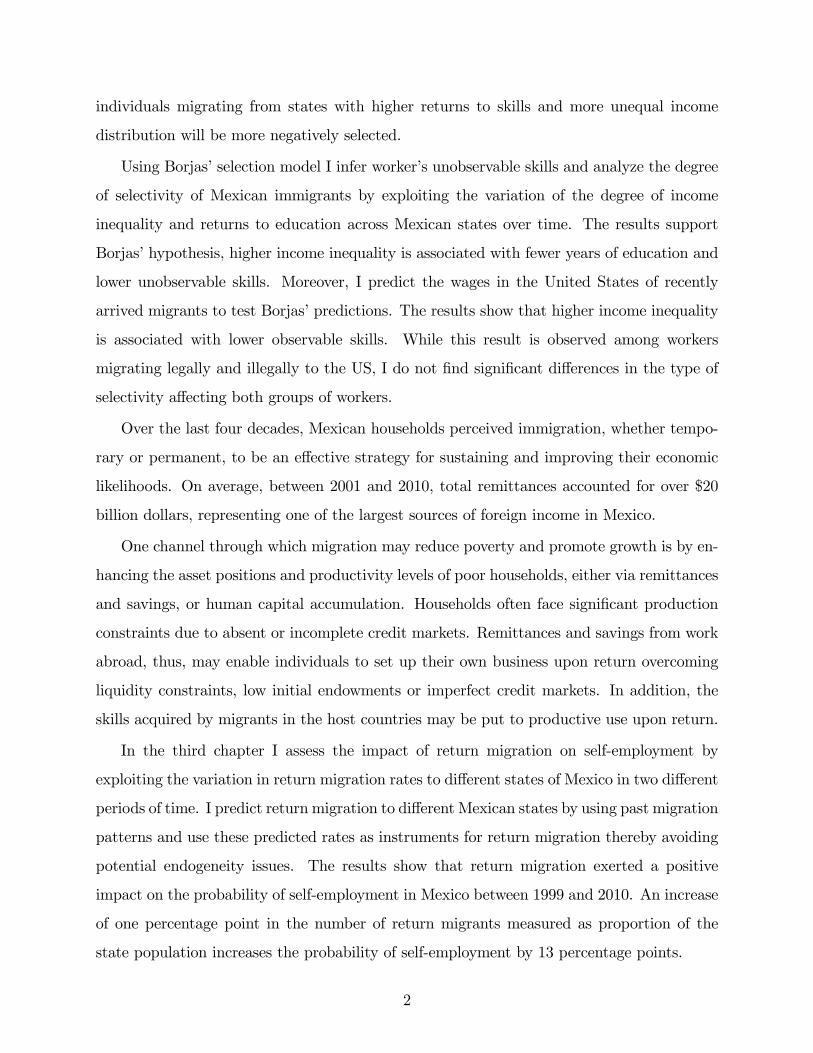
Over the last four decades, Mexican households perceived immigration, whether tempo-

rary or permanent, to be an e¤ective strategy for sustaining and improving their economic

likelihoods. On average, between 2001 and 2010, total remittances accounted for over $20

billion dollars, representing one of the largest sources of foreign income in Mexico.

One channel through which migration may reduce poverty and promote growth is by en-

hancing the asset positions and productivity levels of poor households, either via remittances

and savings, or human capital accumulation. Households often face signi�cant production

constraints due to absent or incomplete credit markets. Remittances and savings from work

abroad, thus, may enable individuals to set up their own business upon return overcoming

liquidity constraints, low initial endowments or imperfect credit markets. In addition, the

skills acquired by migrants in the host countries may be put to productive use upon return.

In the third chapter I assess the impact of return migration on self-employment by

exploiting the variation in return migration rates to di¤erent states of Mexico in two di¤erent

periods of time. I predict return migration to di¤erent Mexican states by using past migration

patterns and use these predicted rates as instruments for return migration thereby avoiding

potential endogeneity issues. The results show that return migration exerted a positive

impact on the probability of self-employment in Mexico between 1999 and 2010. An increase

of one percentage point in the number of return migrants measured as proportion of the

state population increases the probability of self-employment by 13 percentage points.

2

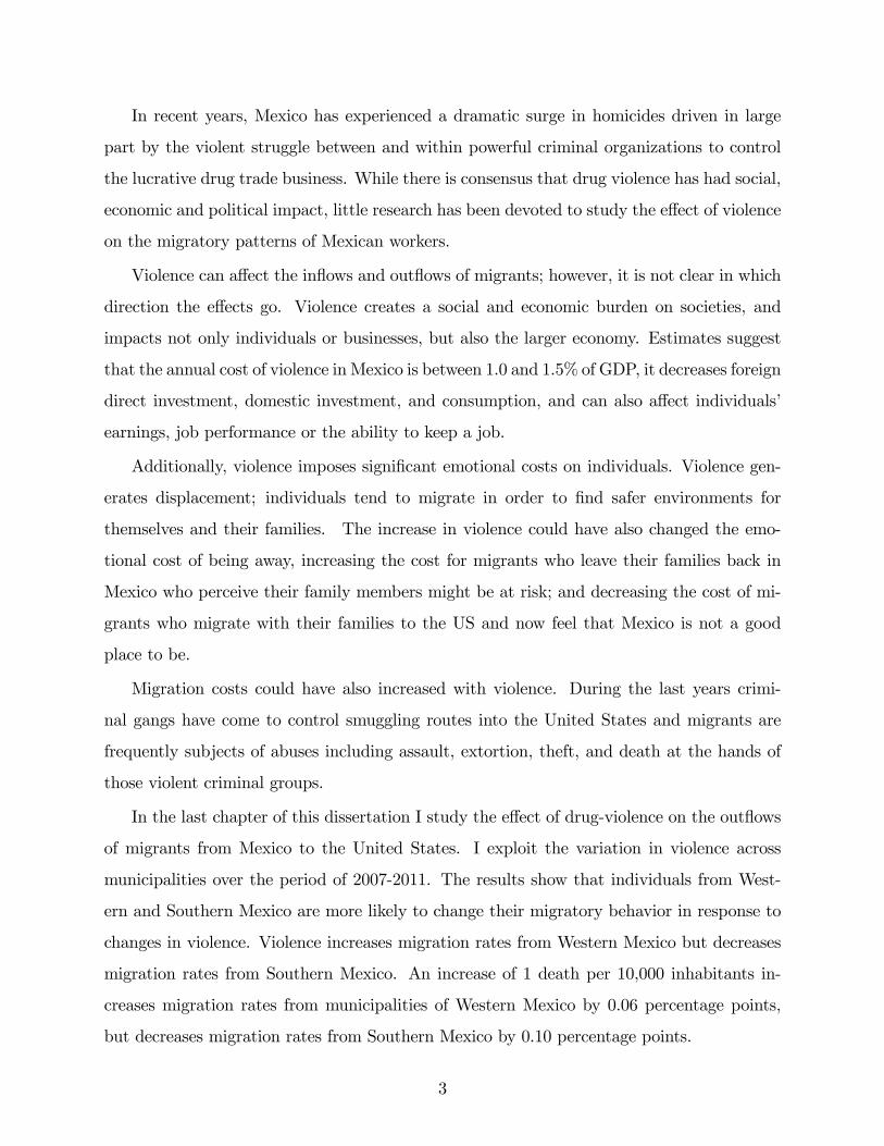
In recent years, Mexico has experienced a dramatic surge in homicides driven in large

part by the violent struggle between and within powerful criminal organizations to control

the lucrative drug trade business. While there is consensus that drug violence has had social,

economic and political impact, little research has been devoted to study the e¤ect of violence

on the migratory patterns of Mexican workers.

Violence can a¤ect the in�ows and out�ows of migrants; however, it is not clear in which

direction the e¤ects go. Violence creates a social and economic burden on societies, and

impacts not only individuals or businesses, but also the larger economy. Estimates suggest

that the annual cost of violence in Mexico is between 1.0 and 1.5% of GDP, it decreases foreign

direct investment, domestic investment, and consumption, and can also a¤ect individuals�

earnings, job performance or the ability to keep a job.

Additionally, violence imposes signi�cant emotional costs on individuals. Violence gen-

erates displacement; individuals tend to migrate in order to �nd safer environments for

themselves and their families. The increase in violence could have also changed the emo-

tional cost of being away, increasing the cost for migrants who leave their families back in

Mexico who perceive their family members might be at risk; and decreasing the cost of mi-

grants who migrate with their families to the US and now feel that Mexico is not a good

place to be.

Migration costs could have also increased with violence. During the last years crimi-

nal gangs have come to control smuggling routes into the United States and migrants are

frequently subjects of abuses including assault, extortion, theft, and death at the hands of

those violent criminal groups.

In the last chapter of this dissertation I study the e¤ect of drug-violence on the out�ows

of migrants from Mexico to the United States. I exploit the variation in violence across

municipalities over the period of 2007-2011. The results show that individuals from West-

ern and Southern Mexico are more likely to change their migratory behavior in response to

changes in violence. Violence increases migration rates from Western Mexico but decreases

migration rates from Southern Mexico. An increase of 1 death per 10,000 inhabitants in-

creases migration rates from municipalities of Western Mexico by 0.06 percentage points,

but decreases migration rates from Southern Mexico by 0.10 percentage points.

3

2.0 SURVEY OF MIGRATION TO THE NORTHERN BORDER (EMIF)

2.1 INTRODUCTION

One of challenges of studying Mexican migration and particularly undocumented migration

to the United States is the lack of information. While migrants are observed in household

datasets conducted in the US such as the Current Population Survey (CPS) or the US

Census, those surveys do not allow us to identify migrants by legal status and are likely to

undercount temporary, circular, and undocumented migrants.

In this chapter I introduce one of the most complete sources of information of Mexican

migrants in the United States. The Survey of Migration to the Northern Border (EMIF) is a

cross sectional survey that has been conducted seventeen times between 1993 and 2012 with

the objective to measure the �ows of migrants between Mexico and the United States. The

EMIF�s survey design is similar to the United Kingdom�s International Passenger Survey, it

samples travelers and distinguish visitors and immigrants1.

EMIF�s sample design is constructed by using two dimensions: space and time. Individ-

uals are selected within a �ow of people that walk through a speci�c location at a speci�c

day and time. That is, an individual is surveyed at one speci�c hour of a speci�c day of a

particular quarter, in a particular location point of one speci�c zone within a border city.

The sampling framework is dynamic; rounds of data collection are conducted regularly for

each quarter of a year; hence, units and weights can change given the nature of the migration

�ows.

The Mexican Department of Labor and Social Welfare estimates that EMIF accounts for

1Brownell (2010).

4

more than 90 percent of migrant �ows between the US and Mexico2. It is conducted among

individuals twelve years of age or older who were not born in the US and who do not live in

the city in which the survey is conducted.

The EMIF consists of four di¤erent questionnaires that quantify the �ows of migrants

going into and out of Mexico. The �rst one is conducted among northward-bound migrants

with destinations in either Mexican border cities or the US; the second one is conducted

among migrants returned to Mexico by the US Border Patrol; the third one is conducted

among southward-bound migrants returning to Mexico from the United States; and �nally,

the fourth questionnaire is conducted among southward-bound migrants from Mexican bor-

der cities.

In this dissertation I use information of the �rst three questionnaires of the EMIF. Each

section contains socioeconomic characteristics of migrants such as age, years of schooling,

marital status, legal status, and state of origin.

The survey conducted among individuals migrating to the US includes information of

their labor market outcomes prior to migration such as employment status, wages or oc-

cupation in Mexico. Additionally the survey asks their motive to migrate and if they had

previous migratory experience. Given the scope of this dissertation, I restrict the sample to

include only individuals migrating to the US to work or look for a job eliminating students

and tourists.

The survey conducted among migrants returning to Mexico includes information of their

duration in the US, state, wages, occupation, and remittance behavior. The survey also asks

their reason to return which allows to identify return migrants and temporary workers. For

individuals who were caught by the Border Patrol the survey includes information of their

place of apprehension and their intentions to try to re-enter the US. For all workers returning

to Mexico (either voluntarily or by the Border Patrol) I restrict the sample to include only

individuals who were in the US to work or look for a job.

While the EMIF is one of the most complete datasets available to study Mexican migra-

tion, the use of its di¤erent sections has to consider the possible selection biases that can

occur given the survey design.

2Secretar¬a de Trabajo y Prevision Social 1999.

5

2.2 MIGRANTS RETURNED BY THE BORDER PATROL

2.2.1 Description, advantages and disadvantages of using this sample

This survey is conducted among workers returned to Mexico by the Border Patrol. This

sample includes individuals who were caught while they were trying to enter the US (74%

caught crossing the border) or when they were already in the US in their home or workplace

(26%). Once individuals are returned to Mexico by the Border Patrol 66% of them decide to

re-enter the US within the next few days3. I use this sample in the chapter "Drug Violence

and Migration Flows" to estimate the e¤ect of violence on the probability to re-enter the

US.

This section of the survey provides sample weights which make the sample representative

total number of migrants returned by the Border Patrol and its estimates are in line with

the statistics presented by US Customs and Border Protection. The agency reported that on

average during the �scal years of 2008 to 2011 the number of apprehensions in the Southwest

Border was 505,000 migrants, and according to the EMIF, during the same period of time

the number of apprehensions was approximately 481,000.

2.3 NORTHWARD-BOUND MIGRANTS WITH DESTINATIONS IN

EITHER MEXICAN BORDER CITIES OR THE US

2.3.1 Description, advantages and disadvantages of using this sample

In this survey I restrict the sample to include Mexican migrants with US destination with

intention to work or look for a job. This sample includes migrants who will try to cross into

the US; however, some of them will not succeed. While this sample is representative of the

population leaving their hometowns who traveled to the US-Mexican border with intention

to enter the US, it overestimates the number of migrants who will end up working in the

United States. Even though the evidence show that a large proportion of workers will try

3If I eliminate those individuals who plan to stay in the border city for a period of time the probabilityof re-entry increases to 72 percent.

6

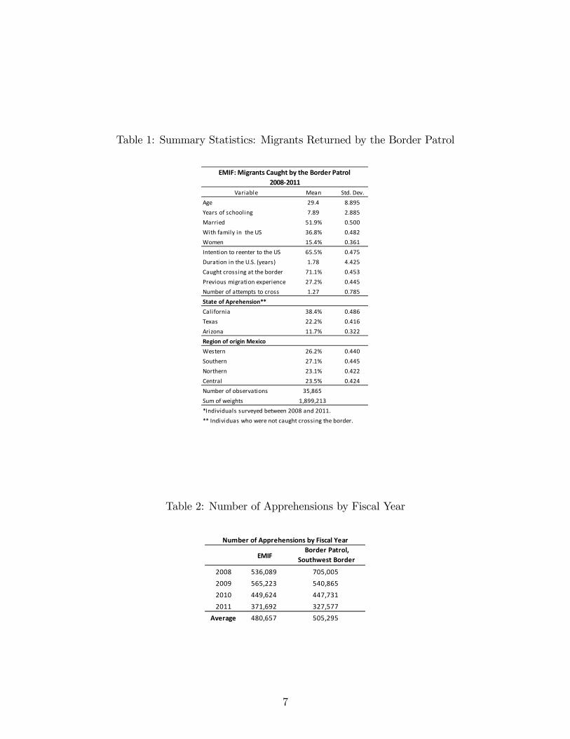
Table 1: Summary Statistics: Migrants Returned by the Border Patrol

Variable Mean Std. Dev.Age 29.4 8.895Years of schooling 7.89 2.885Married 51.9% 0.500With family in  the US 36.8% 0.482Women 15.4% 0.361Intention to reenter to the US 65.5% 0.475Duration in the U.S. (years) 1.78 4.425Caught crossing at the border 71.1% 0.453Previous migration experience 27.2% 0.445Number of attempts to cross 1.27 0.785State of Aprehension**California 38.4% 0.486Texas 22.2% 0.416Arizona 11.7% 0.322Region of origin MexicoWestern 26.2% 0.440Southern 27.1% 0.445Northern 23.1% 0.422Central 23.5% 0.424Number of observations 35,865Sum of weights 1,899,213*Individuals surveyed between 2008 and 2011.** Individuas who were not caught crossing the border.

EMIF: Migrants Caught by the Border Patrol2008­2011

Table 2: Number of Apprehensions by Fiscal Year

EMIFBorder Patrol,

Southwest Border

2008 536,089 705,0052009 565,223 540,8652010 449,624 447,7312011 371,692 327,577

Average 480,657 505,295

Number of Apprehensions by Fiscal Year

7

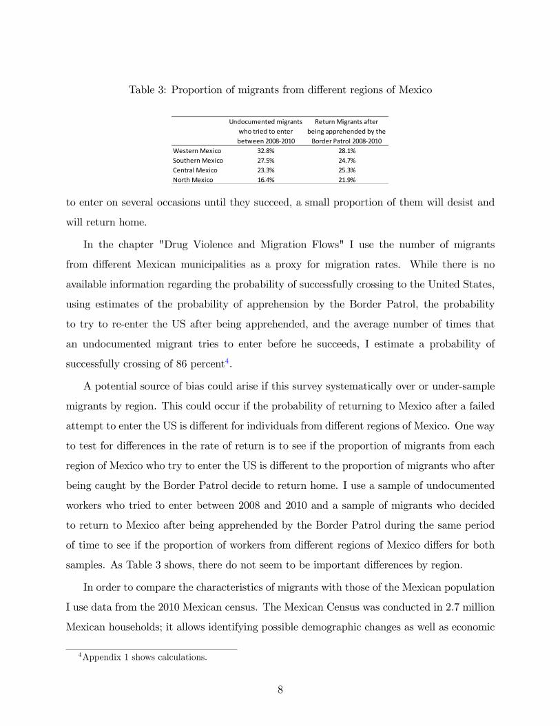
Table 3: Proportion of migrants from di¤erent regions of Mexico

Undocumented migrantswho tried to enterbetween 2008­2010

Return Migrants afterbeing apprehended by the

Border Patrol 2008­2010Western Mexico 32.8% 28.1%Southern Mexico 27.5% 24.7%Central Mexico 23.3% 25.3%North Mexico 16.4% 21.9%

to enter on several occasions until they succeed, a small proportion of them will desist and

will return home.

In the chapter "Drug Violence and Migration Flows" I use the number of migrants

from di¤erent Mexican municipalities as a proxy for migration rates. While there is no

available information regarding the probability of successfully crossing to the United States,

using estimates of the probability of apprehension by the Border Patrol, the probability

to try to re-enter the US after being apprehended, and the average number of times that

an undocumented migrant tries to enter before he succeeds, I estimate a probability of

successfully crossing of 86 percent4.

A potential source of bias could arise if this survey systematically over or under-sample

migrants by region. This could occur if the probability of returning to Mexico after a failed

attempt to enter the US is di¤erent for individuals from di¤erent regions of Mexico. One way

to test for di¤erences in the rate of return is to see if the proportion of migrants from each

region of Mexico who try to enter the US is di¤erent to the proportion of migrants who after

being caught by the Border Patrol decide to return home. I use a sample of undocumented

workers who tried to enter between 2008 and 2010 and a sample of migrants who decided

to return to Mexico after being apprehended by the Border Patrol during the same period

of time to see if the proportion of workers from di¤erent regions of Mexico di¤ers for both

samples. As Table 3 shows, there do not seem to be important di¤erences by region.

In order to compare the characteristics of migrants with those of the Mexican population

I use data from the 2010 Mexican census. The Mexican Census was conducted in 2.7 million

Mexican households; it allows identifying possible demographic changes as well as economic

4Appendix 1 shows calculations.

8

and social. It adds valuable information at di¤erent sampling levels such as municipality,

state and country as a whole. Furthermore, by following the recommendations of interna-

tional institutions and following methodologies widely accepted it collects and organizes the

information such that can be comparable to other countries.

Among the recommendations that are taking into account for designing the Census are

the collection of individual information of all members of the sampling unit; universality, the

process should cover the whole Mexican territory as well as households and people; simul-

taneity, the information is collected at a particular time period; periodicity, it is conducted in

a regular way and time; and, sampling, all surveys conducted during the Census are applied

to sampling units probabilistic selected such that the information is considered representative

of all Mexican territory.

Table 4 shows summary statistics for migrants aged 16 to 65 surveyed by the EMIF

between 2008 and 2011. Table 5 shows summary statistics for the Mexican population

according to the 2010 Mexican Census. If we compare the characteristics of migrants and

the characteristics of the Mexican population we �nd that migrants are slightly younger, less

educated, and predominantly males. With respect to labor market outcomes, migrants are

more likely to be in the labor force, but also more likely to be unemployed prior to migration.

Migrants tend to be disproportionally from Western and Southern Mexico. In this sample

86 percent of the migrants surveyed are undocumented. This estimate is in line with the

calculations presented by the Pew Hispanic Center5.

Next, in order to analyze composition of Mexican migrants according to the state of

origin, and to verify if there exist di¤erences with respect to migrants found in di¤erent

datasets I use a sample of return migrants surveyed by the Mexican Census.

The Census asks respondents two relevant questions. The �rst one is where they had

been living �ve years before the census was taken which allows me to estimate the number

of migrants who returned to Mexico during that period of time. Additionally, in order to

estimate the number of migrants who migrated recently the census asks whether anyone from

the household had left for another country during the previous �ve years. If so, additional

5According to Passel (2006) in the early 2000�s about 80 to 85 percent of the immigrants coming fromMexico entered the U.S. undocumented.

9

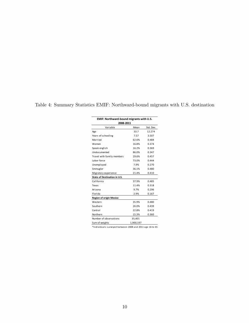
Table 4: Summary Statistics EMIF: Northward-bound migrants with U.S. destination

Variable Mean Std. Dev.Age 33.7 12.274Years of schooling 7.57 3.507Married 62.6% 0.484Women 16.8% 0.374Speak english 16.2% 0.369Undocumented 86.0% 0.347Travel with family members 29.6% 0.457Labor force 73.0% 0.444Unemployed 7.9% 0.270Smmugler 36.1% 0.480Migratory experience 21.4% 0.410State of Destination in U.S.California 37.9% 0.485Texas 11.4% 0.318Arizona 9.7% 0.296Florida 2.9% 0.167Region of origin MexicoWestern 35.9% 0.480Southern 26.0% 0.439Central 22.8% 0.419Northern 15.3% 0.360Number of observations 35,401Sum of weights 1,900,197*Individuals  surveyed between 2008 and 2011 age 16 to 65.

EMIF: Northward­bound migrants with U.S.2008­2011

10

questions are asked about whether and when that person or persons came back.

Between 2005 and 2010, 1.4 million people returned to Mexico, or 1.3 percent of the total

population of 2010. We can group return migrants into di¤erent categories. The �rst and

largest group is Mexican born adults who lived in the US �ve years before and in Mexico

in the census date (812,000 individuals). The second group is US born who were in the US

�ve years before the census and were back in Mexico at the time of the Census (153,000

individuals, largely children). The third one consists of children under 5 born in the US and

in Mexico at the time of the census (203,000 children). Finally, the last group includes recent

migrants, who were in Mexico �ve years before the census, were in Mexico at the time of the

census, but during that period migrated to the US and returned (205,000 individuals).

If the objective is to compare state of origin of migrants surveyed by the EMIF I need

to focus on the �rst group of return migrants, the Mexican adults who were living in the US

in 2005 and were back in Mexico in 2010. The second and third categories include mainly

children, and the fourth category, given the structure of the census, we know the number

of individuals but we do not have information of their individual characteristics and labor

market outcomes.

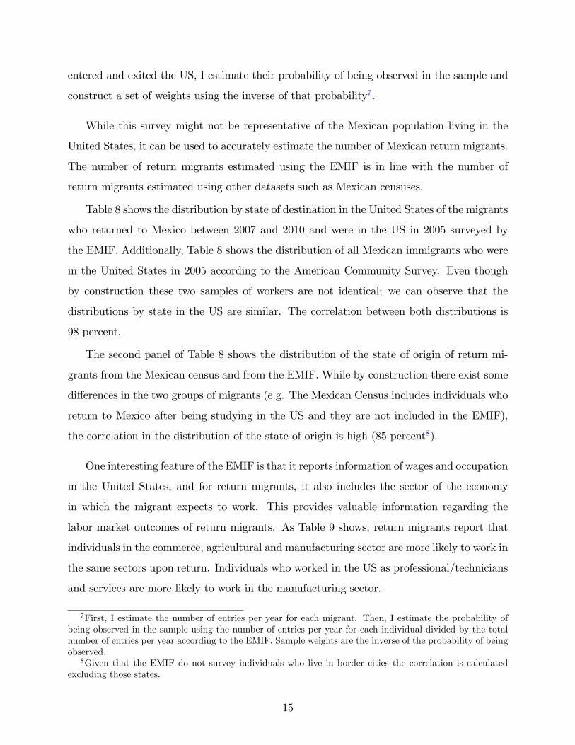
Table 6 shows the distribution by state of origin of the return migrants who were in the

United States in 2005 and in Mexico in 2010 according to the Mexican Census. Additionally,

Table 6 shows the distribution of individuals who migrated and were surveyed by the EMIF

(Northward-bound survey) between 1999 and 2005.

Even though by construction these two samples of workers are not identical, the census

is the only other dataset that allows to study immigrants�state of origin. The correlation

estimated between both distributions is 0.74. While this correlation does not seem very

high, it does not represent a concern since the Mexican Census only identi�es migrants who

returned to Mexico and misses all those who are still in the U.S. at the time of the survey.

As has been shown in the literature, return migration is not a random process, a factor that

could explain the di¤erences found in those distributions.

If I want to compare the characteristics of the migrants found in the Mexican census a

better comparison group would be a sample of return migrants who were in the US in 2005

and in Mexico in 2010. I can �nd migrants with those characteristics using the Southward-

11

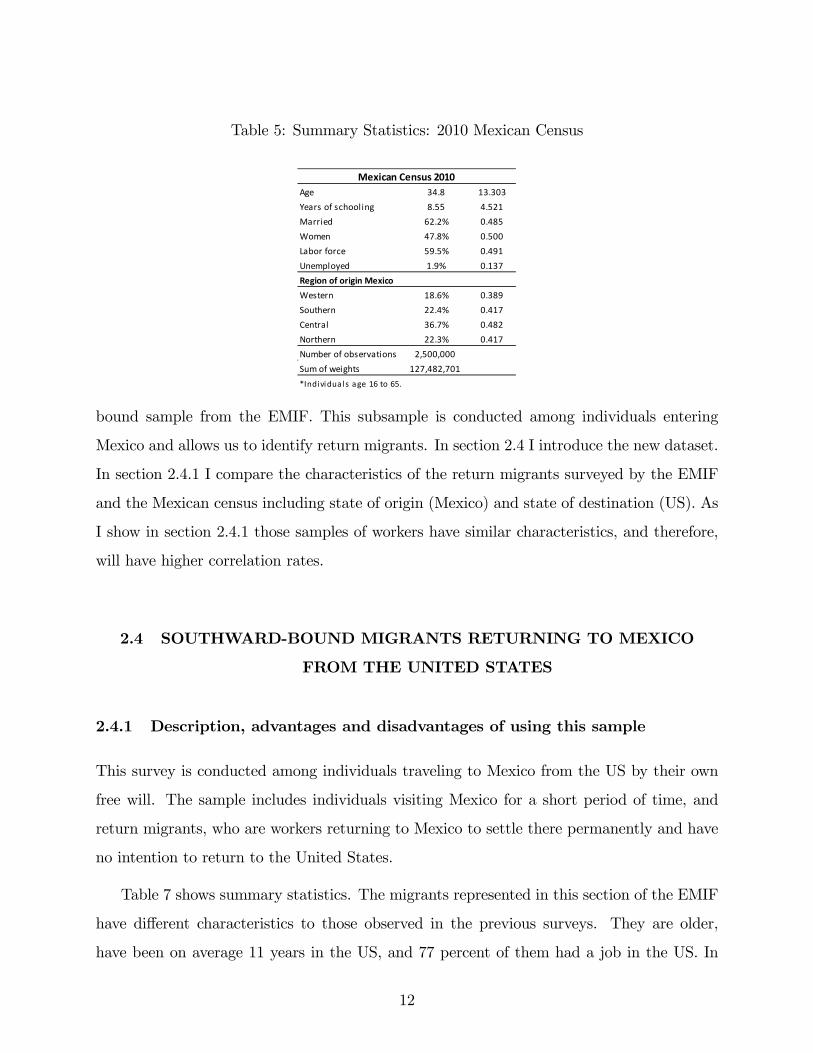
Table 5: Summary Statistics: 2010 Mexican Census

Age 34.8 13.303Years of schooling 8.55 4.521Married 62.2% 0.485Women 47.8% 0.500Labor force 59.5% 0.491Unemployed 1.9% 0.137Region of origin MexicoWestern 18.6% 0.389Southern 22.4% 0.417Central 36.7% 0.482Northern 22.3% 0.417Number of observations 2,500,000Sum of weights 127,482,701*Individuals  age 16 to 65.

Mexican Census 2010

bound sample from the EMIF. This subsample is conducted among individuals entering

Mexico and allows us to identify return migrants. In section 2.4 I introduce the new dataset.

In section 2.4.1 I compare the characteristics of the return migrants surveyed by the EMIF

and the Mexican census including state of origin (Mexico) and state of destination (US). As

I show in section 2.4.1 those samples of workers have similar characteristics, and therefore,

will have higher correlation rates.

2.4 SOUTHWARD-BOUND MIGRANTS RETURNING TO MEXICO

FROM THE UNITED STATES

2.4.1 Description, advantages and disadvantages of using this sample

This survey is conducted among individuals traveling to Mexico from the US by their own

free will. The sample includes individuals visiting Mexico for a short period of time, and

return migrants, who are workers returning to Mexico to settle there permanently and have

no intention to return to the United States.

Table 7 shows summary statistics. The migrants represented in this section of the EMIF

have di¤erent characteristics to those observed in the previous surveys. They are older,

have been on average 11 years in the US, and 77 percent of them had a job in the US. In

12

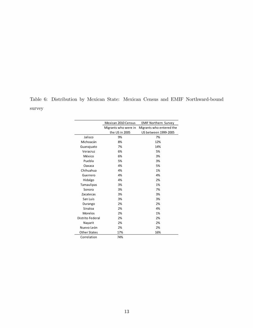
Table 6: Distribution by Mexican State: Mexican Census and EMIF Northward-bound

survey

Mexican 2010 Census EMIF Northern  SurveyMigrants who were in

the US in 2005Migrants who entered the

US between 1999­2005Jalisco 9% 7%

Michoacán 8% 12%Guanajuato 7% 14%

Veracruz 6% 5%México 6% 3%Puebla 5% 3%Oaxaca 4% 5%

Chihuahua 4% 1%Guerrero 4% 4%Hidalgo 4% 2%

Tamaulipas 3% 1%Sonora 3% 7%

Zacatecas 3% 3%San Luis 3% 3%Durango 2% 2%Sinaloa 2% 4%Morelos 2% 1%

Distrito Federal 2% 2%Nayarit 2% 2%

Nuevo León 2% 2%Other States 17% 16%Correlation 74%

13

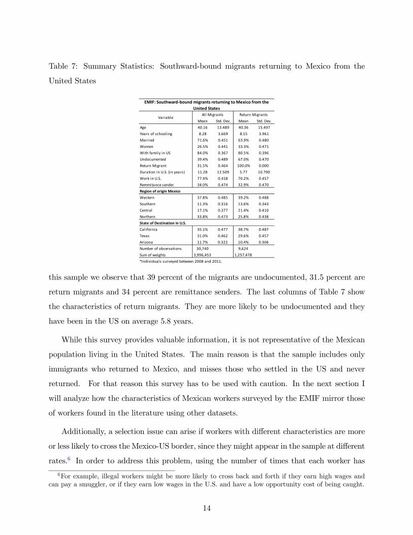
Table 7: Summary Statistics: Southward-bound migrants returning to Mexico from the

United States

Mean Std. Dev. Mean Std. Dev.Age 40.16 13.489 40.36 15.497Years of schooling 8.28 3.669 8.15 3.961Married 71.6% 0.451 63.9% 0.480Women 26.5% 0.441 33.3% 0.471With family in US 84.0% 0.367 80.5% 0.396Undocumented 39.4% 0.489 67.0% 0.470Return Migrant 31.5% 0.464 100.0% 0.000Duration in U.S. (in years) 11.28 12.509 5.77 10.790Work in U.S. 77.4% 0.418 70.2% 0.457Remmitance sender 34.0% 0.474 32.9% 0.470Region of origin MexicoWestern 37.8% 0.485 39.2% 0.488Southern 11.3% 0.316 13.6% 0.343Central 17.1% 0.377 21.4% 0.410Northern 33.8% 0.473 25.8% 0.438State of Destination in U.S.California 35.1% 0.477 38.7% 0.487Texas 31.0% 0.462 29.6% 0.457Arizona 11.7% 0.322 10.4% 0.306Number of observations 30,740 9,624Sum of weights 3,996,453 1,257,478*Individuals surveyed between 2008 and 2011.

EMIF: Southward­bound migrants returning to Mexico from theUnited States

All Migrants Return MigrantsVariable

this sample we observe that 39 percent of the migrants are undocumented, 31.5 percent are

return migrants and 34 percent are remittance senders. The last columns of Table 7 show

the characteristics of return migrants. They are more likely to be undocumented and they

have been in the US on average 5.8 years.

While this survey provides valuable information, it is not representative of the Mexican

population living in the United States. The main reason is that the sample includes only

immigrants who returned to Mexico, and misses those who settled in the US and never

returned. For that reason this survey has to be used with caution. In the next section I

will analyze how the characteristics of Mexican workers surveyed by the EMIF mirror those

of workers found in the literature using other datasets.

Additionally, a selection issue can arise if workers with di¤erent characteristics are more

or less likely to cross the Mexico-US border, since they might appear in the sample at di¤erent

rates.6 In order to address this problem, using the number of times that each worker has

6For example, illegal workers might be more likely to cross back and forth if they earn high wages andcan pay a smuggler, or if they earn low wages in the U.S. and have a low opportunity cost of being caught.

14

entered and exited the US, I estimate their probability of being observed in the sample and

construct a set of weights using the inverse of that probability7.

While this survey might not be representative of the Mexican population living in the

United States, it can be used to accurately estimate the number of Mexican return migrants.

The number of return migrants estimated using the EMIF is in line with the number of

return migrants estimated using other datasets such as Mexican censuses.

Table 8 shows the distribution by state of destination in the United States of the migrants

who returned to Mexico between 2007 and 2010 and were in the US in 2005 surveyed by

the EMIF. Additionally, Table 8 shows the distribution of all Mexican immigrants who were

in the United States in 2005 according to the American Community Survey. Even though

by construction these two samples of workers are not identical; we can observe that the

distributions by state in the US are similar. The correlation between both distributions is

98 percent.

The second panel of Table 8 shows the distribution of the state of origin of return mi-

grants from the Mexican census and from the EMIF. While by construction there exist some

di¤erences in the two groups of migrants (e.g. The Mexican Census includes individuals who

return to Mexico after being studying in the US and they are not included in the EMIF),

the correlation in the distribution of the state of origin is high (85 percent8).

One interesting feature of the EMIF is that it reports information of wages and occupation

in the United States, and for return migrants, it also includes the sector of the economy

in which the migrant expects to work. This provides valuable information regarding the

labor market outcomes of return migrants. As Table 9 shows, return migrants report that

individuals in the commerce, agricultural and manufacturing sector are more likely to work in

the same sectors upon return. Individuals who worked in the US as professional/technicians

and services are more likely to work in the manufacturing sector.

7First, I estimate the number of entries per year for each migrant. Then, I estimate the probability ofbeing observed in the sample using the number of entries per year for each individual divided by the totalnumber of entries per year according to the EMIF. Sample weights are the inverse of the probability of beingobserved.

8Given that the EMIF do not survey individuals who live in border cities the correlation is calculatedexcluding those states.

15

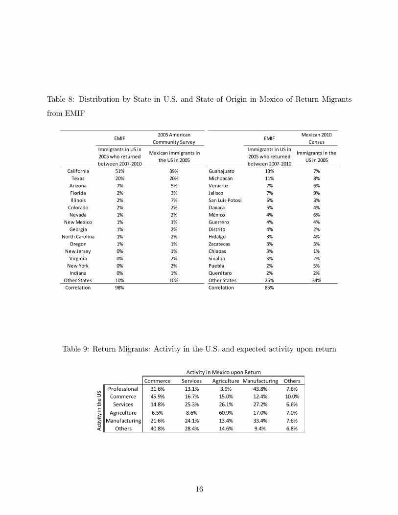
Table 8: Distribution by State in U.S. and State of Origin in Mexico of Return Migrants

from EMIF

EMIF2005 American

Community SurveyEMIF

Mexican 2010Census

Immigrants in US in2005 who returnedbetween 2007­2010

 Mexican immigrants inthe US in 2005

Immigrants in US in2005 who returnedbetween 2007­2010

Immigrants in theUS in 2005

California 51% 39% Guanajuato 13% 7%Texas 20% 20% Michoacán 11% 8%

Arizona 7% 5% Veracruz 7% 6%Florida 2% 3% Jalisco 7% 9%Illinois 2% 7% San Luis Potosi 6% 3%

Colorado 2% 2% Oaxaca 5% 4%Nevada 1% 2% México 4% 6%

New Mexico 1% 1% Guerrero 4% 4%Georgia 1% 2% Distrito 4% 2%

North Carolina 1% 2% Hidalgo 3% 4%Oregon 1% 1% Zacatecas 3% 3%

New Jersey 0% 1% Chiapas 3% 1%Virginia 0% 2% Sinaloa 3% 2%

New York 0% 2% Puebla 2% 5%Indiana 0% 1% Querétaro 2% 2%

Other States 10% 10% Other States 25% 34%Correlation 98% Correlation 85%

Table 9: Return Migrants: Activity in the U.S. and expected activity upon return

Commerce Services Agriculture Manufacturing OthersProfessional 31.6% 13.1% 3.9% 43.8% 7.6%Commerce 45.9% 16.7% 15.0% 12.4% 10.0%

Services 14.8% 25.3% 26.1% 27.2% 6.6%Agriculture 6.5% 8.6% 60.9% 17.0% 7.0%

Manufacturing 21.6% 24.1% 13.4% 33.4% 7.6%Others 40.8% 28.4% 14.6% 9.4% 6.8%

Activity in Mexico upon Return

Activ

ity in

 the 

US

16

2.4.2 Return Migration: EMIF and Mexican census data

I analyze how the characteristics of the return migrants observed in the EMIF compares

to those of return migrants captured by other datasets. I choose the 2010 Mexican Census

to conduct the analysis for several reasons. First, as it has been pointed out by di¤erent

authors9, from all the di¤erent datasets that include return migrants and identi�es them, the

2010 Mexican Census provides questions that can be used to make an accurate estimation

of their number.

In order to compare the census data I select all return migrants from the EMIF who

migrated and returned to Mexico during the same period of time. The results are shown

in Tables 10 and 11. The Census reports 811,725 return migrants and the EMIF reports

806,267. The results also show some di¤erences across samples. According to the census,

return migrants are on average younger and more educated. The proportion of women is

higher, and 11.4 percent of the respondents report to work in professional activities.

One reason that could explain the di¤erent characteristics observed is that the EMIF

tends to underestimate the number of individuals who studied in the US and returned to

Mexico. When I look at the proportion of return migrants with more than sixteen years

of schooling (with Masters or Ph.D. degrees) the EMIF captures less than �fty percent of

those observed in the Census. It is important to note that those individuals represent a

small share of the total number of return migrants. According to the census 4 percent of the

return migrants have more than 16 years of schooling and only 2 percent according to the

EMIF. Unfortunately, the census does not provide information on the reason to migrate to

the United States, therefore we cannot di¤erentiate between individuals who migrate with

intention to work in the US.

For those reasons, the EMIF becomes the best source of information about return migra-

tion given that my objective is to study the e¤ects of migration to the United States to work

or look for a job. This dataset is used in the chapter "Testing Borjas�Negative Selection

Hypothesis among Mexican Immigrants in the United States" and in the chapter "Return

Migration and Self-Employment in Mexico. In the latest I further restrict the sample to only

9Passel, Cohn and Gonzalez-Barrera (2012).

17

include return migrants who actually worked in the United States.

2.4.3 Survey of Migration to the Northern Border (EMIF) and Current Popu-

lation Survey (CPS)

I examine how the characteristics of Mexican workers surveyed by the EMIF mirror those

of workers found in the literature using other datasets. I use information from the CPS

available since 1994. I compare the characteristics of Mexican workers from the CPS with

those of legal workers settled permanently in the US from the EMIF and �nd no signi�cant

di¤erences in their education and wages. These results suggest that, even though the EMIF

only includes Mexican workers who returned to Mexico and misses the workers who never

returned, the characteristics of legal permanent workers observed in the EMIF are similar

to those of the workers survey by the CPS, a survey that includes a representative sample

of the Mexican workers permanently settled in the United States.

Figure 1 shows average hourly earnings for di¤erent cohorts of Mexican male migrants

from the CPS, and Figure 2 shows average hourly earnings of workers from the EMIF. When

we compare all workers from both surveys (Figures 1 and 2) we can observe similar trends

in their wages, however, the wages from the EMIF are lower for all cohorts of entry.

Given that the likelihood of observing illegal and temporary workers is lower in the CPS

than in the EMIF, and that those groups of workers are the ones more likely to earn lower

wages, I also compare the trends on the wages observed from the CPS with the wages of

legal workers settled permanently in the US from the EMIF (Figure 3). Now there are not

di¤erences in the wages of workers who entered before 1990, and for the two most recent

cohorts, the wages from the EMIF are even higher than those observed from the CPS. These

results suggest that, even though the EMIF only includes Mexican workers who return to

Mexico and misses the workers who never return, the wages of legal permanent workers

observed in the EMIF are similar to those of the workers survey by the CPS, a survey that

includes a representative sample of the Mexican workers permanently settled in the US.

These results were replicated for di¤erent age categories obtaining similar results.

18

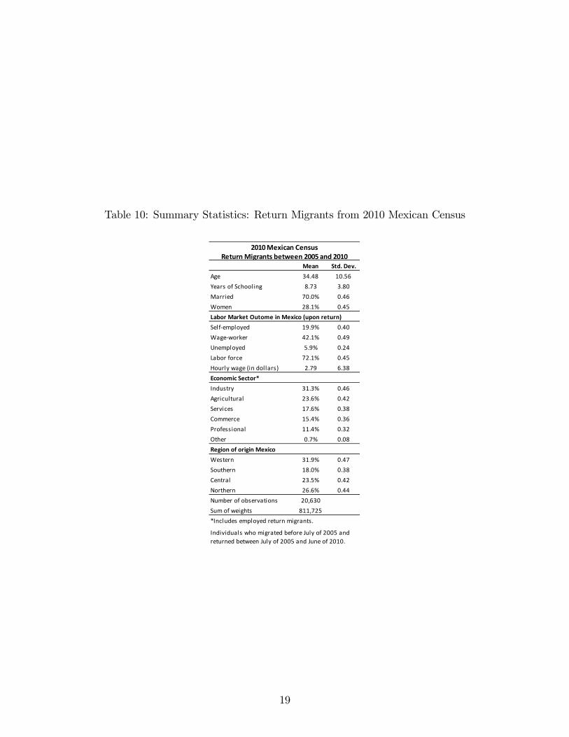
Table 10: Summary Statistics: Return Migrants from 2010 Mexican Census

Mean Std. Dev.Age 34.48 10.56Years of Schooling 8.73 3.80Married 70.0% 0.46Women 28.1% 0.45Labor Market Outome in Mexico (upon return)Self­employed 19.9% 0.40Wage­worker 42.1% 0.49Unemployed 5.9% 0.24Labor force 72.1% 0.45Hourly wage (in dollars) 2.79 6.38Economic Sector*Industry 31.3% 0.46Agricultural 23.6% 0.42Services 17.6% 0.38Commerce 15.4% 0.36Professional 11.4% 0.32Other 0.7% 0.08Region of origin MexicoWestern 31.9% 0.47Southern 18.0% 0.38Central 23.5% 0.42Northern 26.6% 0.44Number of observations 20,630Sum of weights 811,725*Includes employed return migrants.

Return Migrants between 2005 and 20102010 Mexican Census

Individuals who migrated before July of 2005 andreturned between July of 2005 and June of 2010.

19

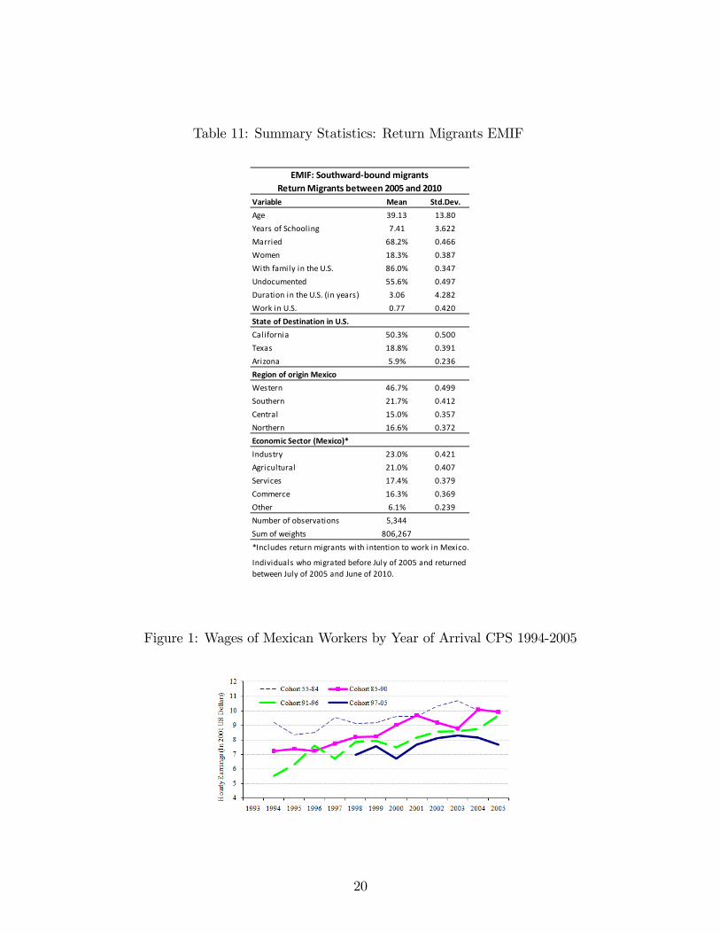
Table 11: Summary Statistics: Return Migrants EMIF

Variable Mean Std.Dev.Age 39.13 13.80Years of Schooling 7.41 3.622Married 68.2% 0.466Women 18.3% 0.387With family in the U.S. 86.0% 0.347Undocumented 55.6% 0.497Duration in the U.S. (in years) 3.06 4.282Work in U.S. 0.77 0.420State of Destination in U.S.California 50.3% 0.500Texas 18.8% 0.391Arizona 5.9% 0.236Region of origin MexicoWestern 46.7% 0.499Southern 21.7% 0.412Central 15.0% 0.357Northern 16.6% 0.372Economic Sector (Mexico)*Industry 23.0% 0.421Agricultural 21.0% 0.407Services 17.4% 0.379Commerce 16.3% 0.369Other 6.1% 0.239Number of observations 5,344Sum of weights 806,267*Includes return migrants with intention to work in Mexico.

EMIF: Southward­bound migrantsReturn Migrants between 2005 and 2010

Individuals who migrated before July of 2005 and returnedbetween July of 2005 and June of 2010.

Figure 1: Wages of Mexican Workers by Year of Arrival CPS 1994-2005

20

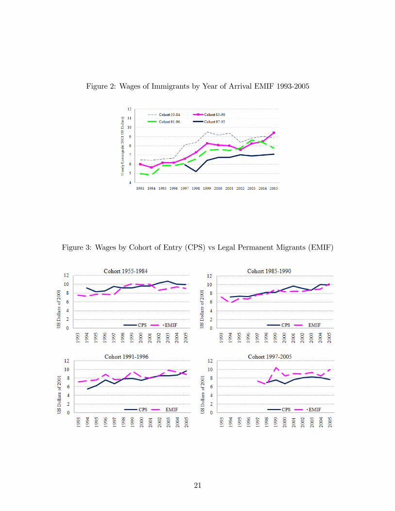
Figure 2: Wages of Immigrants by Year of Arrival EMIF 1993-2005

Figure 3: Wages by Cohort of Entry (CPS) vs Legal Permanent Migrants (EMIF)

21

3.0 TESTING BORJAS�NEGATIVE SELECTION HYPOTHESIS AMONG

MEXICAN IMMIGRANTS IN THE UNITED STATES

3.1 MOTIVATION

International migration is a selective process, and a key prediction of economic theory is

that the labor market impact of immigration hinges crucially on how the skills of immigrants

compare to those of natives in the host country.

Borjas (1987) provides a theoretical and empirical framework that speci�es conditions

under which immigrants could be either positively or negatively selected. According to

his model, individuals with the greatest incentive to migrate to the United States from

countries with high returns to education and relatively high dispersion of wages will tend

to be those with below-average skill levels in their home countries (negatively selected).

On the other hand, the immigrants who �nd it pro�table to migrate from countries where

returns to education and wage dispersion are relatively low will tend to be individuals with

above-average skills (positively selected). Borjas (1987) analyzes empirically the di¤erences

in earnings of immigrants from 41 countries and studies the relationship between income

inequality in their countries of origin and their earnings in the United States. He �nds that

immigrants with high incomes in the United States relative to their measured skills come

from countries that have high levels of GNP, low levels of income inequality and politically

competitive systems.

While most of the research on selectivity of immigrants has studied the earnings of

immigrants in the United States, I study the selectivity of immigrants but using evidence

from a source country. In this paper I study the selectivity of Mexican immigrants in the

22

United States. Mexico is the largest source of immigrants for the United States, today 58%

of the undocumented population in the United States is of Mexican origin (6.5 millions), and

30% of the total foreign born population (11.5 millions)1.

In this paper I test Borjas�1987 negative selection hypothesis which states that indi-

viduals migrating from states with more unequal income distribution, with high returns to

education and relatively high dispersion of wages will be more negatively selected. I exploit

the variation of the degree of income inequality and returns to education across states in

Mexico and over time to test for di¤erences in the type of selectivity observed among legal

and illegal immigrants. First, I analyze selectivity in terms of years of schooling. Then,

using Borjas�selection model I infer worker�s unobservable skills and analyze the degree of

selectivity based on observable and unobservable skills. Moreover, I predict the wages in the

United States of recently arrived Mexican migrants to test Borjas�predictions. I control for

migration costs and the size of immigrants�social networks, two important factors likely to

in�uence immigrants�selectivity.

I use data of Mexican immigrants from the Survey of Migration to the Northern Border

(EMIF). This survey was conducted between 1995 and 2005, it provides information of

wages prior to migration and wages earned in the United States, identi�es immigrants by

legal status, and is conducted between temporary and permanent immigrants. The use of

this survey allows me to overcome a number of shortcomings observed in previous studies

due in large measure to the limitations of the census data that has been the principal data

source for research on the selectivity of immigrants. First, I study selectivity using earnings

prior to migration and earnings in the United States. Previous studies only used earnings

of new immigrants in the United States which confound both, skill selectivity and initial

skill transferability. Second, I identify workers by legal status. Immigrants�participation

in the US labor market is subject to di¤erent constraints depending on visa status. Census

data do not provide information of the individual�s legal status, making it di¢ cult to draw

inferences about the skill selectivity of workers. Third, the dataset used in this paper is

conducted among workers temporarily and permanently settled in the United States. If

1Pew Hispanic Center (2011). "Statistical Portraits of the Hispanic and Foreign-Born Populations in theU.S.

23

return migration is not accounted for, due to the selectivity of emigration, the comparison

of an aggregate immigrant cohort in two time periods confounds the skill transferability of

an individual over time and changes in the skill composition of immigrants.

When I study years of education, while aggregate analysis �nd evidence of positive, inter-

mediate and negative selection in di¤erent periods of time, once we control for compositional

e¤ects we �nd evidence of negative selection of Mexican migrants at the state and region

level over the period of analysis.

When I study earnings prior to migration I �nd evidence of negative selection of Mexican

immigrants in terms of unobservable skills. Higher income inequality in the state of origin

in Mexico is associated with lower unobservable skills. Finally, when I study earnings in

the United States the results also support Borjas� prediction. Higher income inequality

is associated with lower observable skills of workers migrating legally and illegally to the

US. Even though the results show that both groups of workers behave according to Borjas�

hypothesis, the evidence shows that there are no signi�cant di¤erences in the degree of

selectivity a¤ecting both groups of workers.

3.2 LITERATURE REVIEW

Scholars have disagreed considerably about how immigrants compare to individuals who stay

at their origin country. Human capital models of migration claim that those who choose

to leave a country might be more able and/or more motivated than those who choose to

stay in their home country (Chiswick, 2000, Portes and Rumbaut, 1996). Thus, poor and

uneducated individuals, due to lack of awareness or means, are less likely to migrate than

those who have some education or have learned of the better conditions of living available to

migrants. Another argument is that migration involves cost either economic, or emotional

or both. These obstacles contribute for a high selection given that individuals who are in the

lowest tail of income distribution seldom could a¤ord these costs (Lee, 1966; Schultz, 1984).

Finally, social networks made by earlier waves of immigrants can also a¤ect the degree of

selectivity by decreasing the economic and emotional costs of migration for potential new

24

immigrants. These lower costs can incentive less skilled individuals to migrate (Massey 1987,

1999).

Borjas (1987) by formalizing and extending Roy�s model (1951) speci�es conditions un-

der which immigrants could be either positively or negatively selected. His model predicts

negative selection of immigrants from countries with a great dispersion in income to coun-

tries with a more egalitarian income distribution, whereas positive selection will exist in the

opposite case. Borjas argues that skilled Mexicans do not migrate to the US, since their

skills could be well-paid in their country compared with unskilled Mexican workers. Thus,

unskilled Mexicans facing disadvantages in Mexico are more likely to migrate. Borjas (1987)

also analyzes empirically the di¤erences in earnings of immigrants from 41 countries using

the 1970 and 1980 US censuses. He studies the relationship between income inequality in

their countries of origin and their earnings in the United States. He �nds that immigrants

with high incomes in the United States relative to their measured skills come from countries

that have high levels of GNP, low levels of income inequality and politically competitive

systems.

Relative to the selectivity of Mexican workers most of the research has been devoted to

measure the relative skills of Mexican immigrants in the United States and the empirical

evidence has shown ambiguous results. Chiquiar and Hanson (2005) �nd evidence of inter-

mediate or positive selection in terms of education and observed skills using data from the

1990 Mexican and US censuses. They modify Borjas�model by changing the assumption

of constant migration costs across individuals allowing migration cost to vary by individual

and to decrease with years of schooling. They �nd that Mexican immigrants, while much

less educated than US natives, were on average more educated than residents of Mexico.

Moreover, they �nd that in 1990, if Mexican immigrants in the United States were to be

paid according to current skill prices in Mexico, they would tend to occupy the middle and

upper portions of Mexico�s wage distribution. Similarly, Orrenius and Zavodny (2005) �nd

evidence of intermediate selection in terms of education but using data from the Mexican

Migration Project, a survey conducted in states of Western Mexico between 1987 and 1997.

On the other hand, Ibarraran and Lubotsky (2007) �nd evidence of negative selection

25

in terms of years schooling using data from the 2000 Mexican and US censuses. Fernandez-

Huertas (2011) �nds evidence of intermediate to negative selection in terms of schooling and

wages using data from the Quarterly Employment Survey (ENET). McKenzie and Rapaport

(2010) using the 1997 National Survey of the Demographic Dynamics (ENADID) �nd positive

and negative selection for Mexican immigrants coming from high and low migration rate

communities respectively, and �nally, Kaestner and Malamud (2010) using data from the

Mexican Family Life Survey (MxFLS) �nd no selection in terms of observed and unobserved

skills once they control for migration cost. It has been argued in the immigration literature

that the lack of consensus relative to the type of selectivity a¤ecting Mexican immigrants

can be associated to the assumptions used to adjust the size of the illegal population present

in the di¤erent datasets, to di¤erences in the period of analysis covered by di¤erent studies,

and �nally, to the selectivity associated with return migration if the samples of immigrants

do not include temporary and permanent immigrants.

3.3 DATA

The analysis uses data from the 1990 and 2000 Mexican censuses, the 1995 Population

and Dwelling Count, and the Southward-bound sample of the EMIF that includes migrants

returning to Mexico from the US.

In order to avoid problems associated with selective return migration, I restrict the

sample to include only workers who migrated to the US between 1990 and 20052. Moreover,

I limit my analysis to individuals who were working prior to migration, reported their wages

in Mexico, and who worked in the US for at least one month.

Table 12 shows descriptive statistics. Immigrants have on average 6.4 years of schooling,

were on average 23 years old at the time of entry, and 11.5 percent entered legally to the

United States. With respect to their occupation in Mexico, they were working mainly in

the production and agricultural sectors, and were earning on average 12.25 pesos per hour

2Even though the survey includes immigrants who migrated to the United States between 1950 and 2005,I restrict the sample to include only workers who migrated between 1990 and 2005. Including immigrantswho entered prior that period could potentially bias the results if return migrants are not randomly selected.In the survey workers who returned to Mexico between 1950 and 1990 are not represented.

26

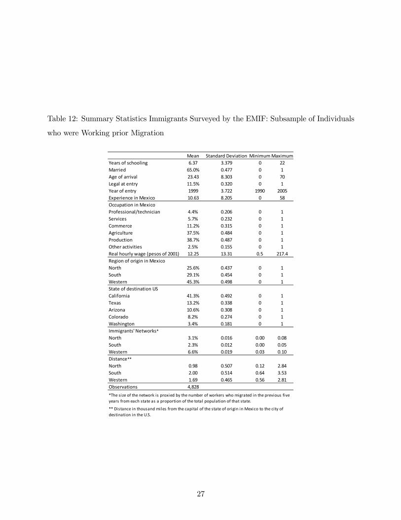
Table 12: Summary Statistics Immigrants Surveyed by the EMIF: Subsample of Individuals

who were Working prior Migration

Mean Standard Deviation Minimum MaximumYears of schooling 6.37 3.379 0 22Married 65.0% 0.477 0 1Age of arrival 23.43 8.303 0 70Legal at entry 11.5% 0.320 0 1Year of entry 1999 3.722 1990 2005Experience in Mexico 10.63 8.205 0 58Occupation in MexicoProfessional/technician 4.4% 0.206 0 1Services 5.7% 0.232 0 1Commerce 11.2% 0.315 0 1Agriculture 37.5% 0.484 0 1Production 38.7% 0.487 0 1Other activities 2.5% 0.155 0 1Real hourly wage (pesos of 2001) 12.25 13.31 0.5 217.4Region of origin in MexicoNorth 25.6% 0.437 0 1South 29.1% 0.454 0 1Western 45.3% 0.498 0 1State of destination USCalifornia 41.3% 0.492 0 1Texas 13.2% 0.338 0 1Arizona 10.6% 0.308 0 1Colorado 8.2% 0.274 0 1Washington 3.4% 0.181 0 1Immigrants' Networks*North 3.1% 0.016 0.00 0.08South 2.3% 0.012 0.00 0.05Western 6.6% 0.019 0.03 0.10Distance**North 0.98 0.507 0.12 2.84South 2.00 0.514 0.64 3.53Western 1.69 0.465 0.56 2.81Observations 4,828*The size of the network is proxied by the number of workers who migrated in the previous fiveyears from each state as a proportion of the total population of that state.

** Distance in thousand miles from the capital of the state of origin in Mexico to the city ofdestination in the U.S.

27

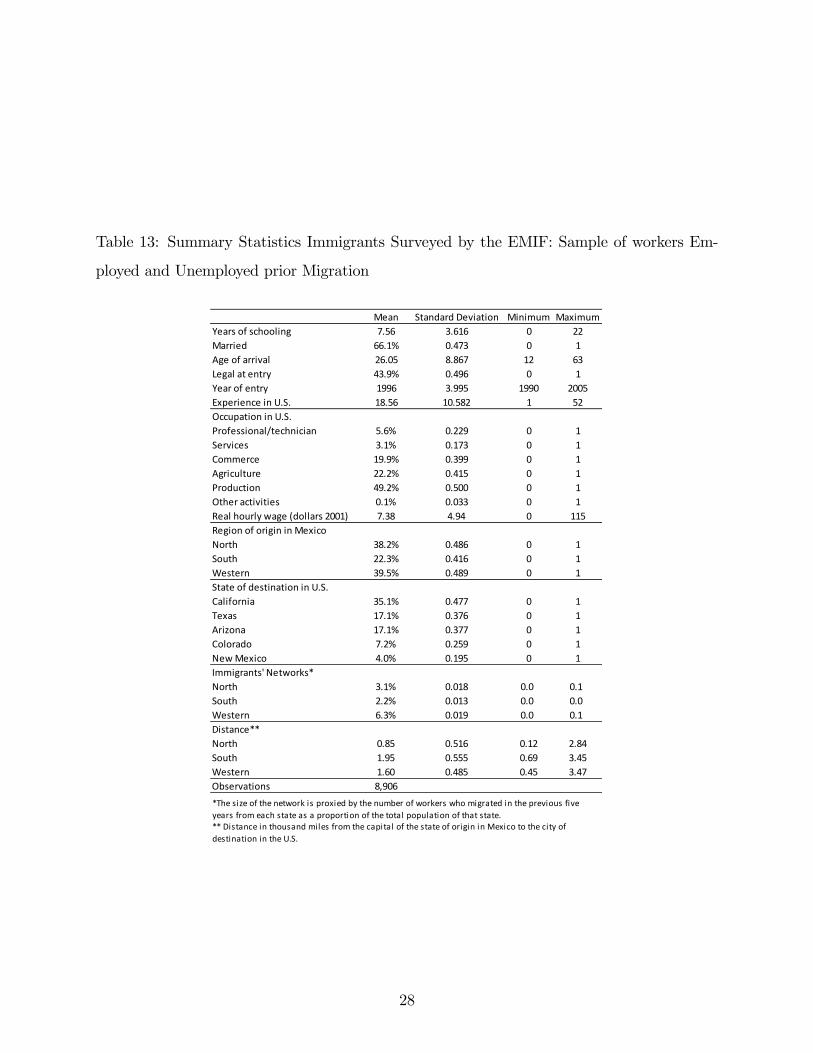
Table 13: Summary Statistics Immigrants Surveyed by the EMIF: Sample of workers Em-

ployed and Unemployed prior Migration

Mean Standard Deviation Minimum MaximumYears of schooling 7.56 3.616 0 22Married 66.1% 0.473 0 1Age of arrival 26.05 8.867 12 63Legal at entry 43.9% 0.496 0 1Year of entry 1996 3.995 1990 2005Experience in U.S. 18.56 10.582 1 52Occupation in U.S.Professional/technician 5.6% 0.229 0 1Services 3.1% 0.173 0 1Commerce 19.9% 0.399 0 1Agriculture 22.2% 0.415 0 1Production 49.2% 0.500 0 1Other activities 0.1% 0.033 0 1Real hourly wage (dollars 2001) 7.38 4.94 0 115Region of origin in MexicoNorth 38.2% 0.486 0 1South 22.3% 0.416 0 1Western 39.5% 0.489 0 1State of destination in U.S.California 35.1% 0.477 0 1Texas 17.1% 0.376 0 1Arizona 17.1% 0.377 0 1Colorado 7.2% 0.259 0 1New Mexico 4.0% 0.195 0 1Immigrants' Networks*North 3.1% 0.018 0.0 0.1South 2.2% 0.013 0.0 0.0Western 6.3% 0.019 0.0 0.1Distance**North 0.85 0.516 0.12 2.84South 1.95 0.555 0.69 3.45Western 1.60 0.485 0.45 3.47Observations 8,906*The size of the network is proxied by the number of workers who migrated in the previous fiveyears from each state as a proportion of the total population of that state.** Distance in thousand miles from the capital of the state of origin in Mexico to the city ofdestination in the U.S.

28

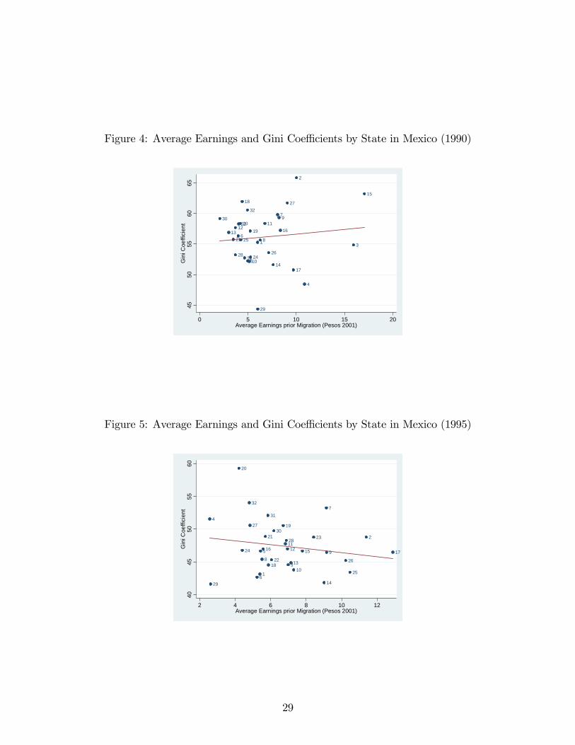
Figure 4: Average Earnings and Gini Coe¢ cients by State in Mexico (1990)

1

2

3

4

5

6

7

8

9

10

1112

13

14

15

16

17

18

1920

21

22

24

25

26

27

28

29

30

31

32

4550

5560

65G

ini C

oeffi

cien

t

0 5 10 15 20Average Earnings prior Migration (Pesos 2001)

Figure 5: Average Earnings and Gini Coe¢ cients by State in Mexico (1995)

1

2

3

4

5

6

7

89

10

1112

13

14

151617

18

19

20

21

22

23

24

25

26

27

28

29

30

31

32

4045

5055

60G

ini C

oeffi

cien

t

2 4 6 8 10 12Average Earnings prior Migration (Pesos 2001)

29

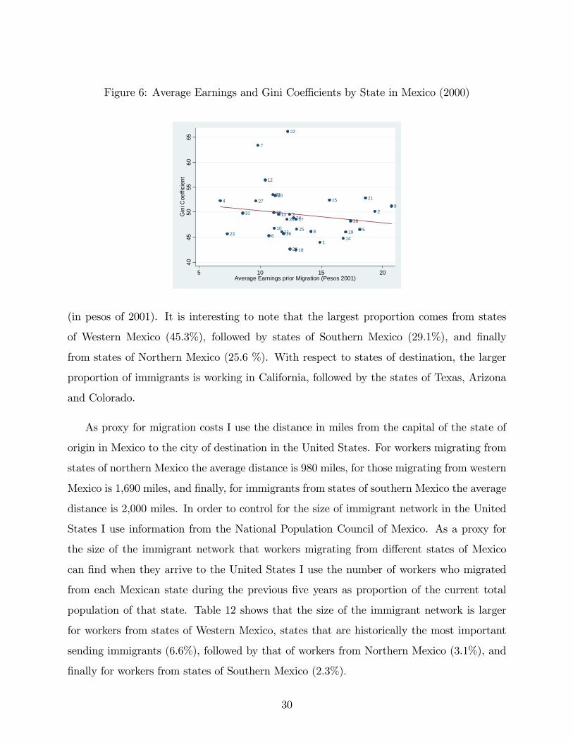
Figure 6: Average Earnings and Gini Coe¢ cients by State in Mexico (2000)

1

23

4

56

7

8

9

1011

12

13

14

15

16

17

18

19

20

21

22

23

24

25

26

27

28

29

30

31

3240

4550

5560

65G

ini C

oeffi

cien

t

5 10 15 20Average Earnings prior Migration (Pesos 2001)

(in pesos of 2001). It is interesting to note that the largest proportion comes from states

of Western Mexico (45.3%), followed by states of Southern Mexico (29.1%), and �nally

from states of Northern Mexico (25.6 %). With respect to states of destination, the larger

proportion of immigrants is working in California, followed by the states of Texas, Arizona

and Colorado.

As proxy for migration costs I use the distance in miles from the capital of the state of

origin in Mexico to the city of destination in the United States. For workers migrating from

states of northern Mexico the average distance is 980 miles, for those migrating from western

Mexico is 1,690 miles, and �nally, for immigrants from states of southern Mexico the average

distance is 2,000 miles. In order to control for the size of immigrant network in the United

States I use information from the National Population Council of Mexico. As a proxy for

the size of the immigrant network that workers migrating from di¤erent states of Mexico

can �nd when they arrive to the United States I use the number of workers who migrated

from each Mexican state during the previous �ve years as proportion of the current total

population of that state. Table 12 shows that the size of the immigrant network is larger

for workers from states of Western Mexico, states that are historically the most important

sending immigrants (6.6%), followed by that of workers from Northern Mexico (3.1%), and

�nally for workers from states of Southern Mexico (2.3%).

30

Migrants were grouped by year of arrival into 3 categories. For individuals who migrated

between 1990 and 1992 their year of reference is 1990, for those who entered between 1993

and 1997 their year of reference is 1995, and for those who entered between 1998 and 2005

their year of reference is 2000. Figures 4 to 6 show the Gini coe¢ cient for Mexican states

and immigrants�earnings prior to migration for years 1990, 1995 and 2000. The �gures show

that without controlling for workers�characteristics, there seems to be a positive relationship

between the income inequality in the state of origin (a Gini coe¢ cient closes to 1 implies

higher inequality) and the earnings of immigrants in 1990, but a negative relationship in

years 1995 and 2000.

In order to estimate the selectivity of immigrants by using wages in the United States I

use a di¤erent sample of workers. The new sample includes more observations since now I

eliminate the restriction of working prior to migration. It includes all workers who migrated

to the United States between 1990 and 2005, who stayed in the US at least six months,

worked in the US and reported their earnings. Table 13 shows descriptive statistics for the

second sample of immigrants. Finally, when I study selectivity of education the sample is

the largest since all the restrictions are eliminated.

3.4 SELECTIVITY IN TERMS OF OBSERVABLE SKILLS

3.4.1 Model

In this section the objective is to test for selectivity in terms of education. I use for the

analysis a simple two country model of migration similar to the one presented by Hanson

and Chiquiar (2005)3. In this model there are two countries, the home country (Mexico) that

will be identi�ed as country 0, and the host country (United States) that will be identi�ed

as country 1. In the model residents of Mexico have the following wage equation:

lnw0 = �0 + �0s (3.1)

3In this model I assume constant migration costs and Hanson and Chiquiar assume that migration costsdecrease with years of schooling.

31

where w0 is the wage in Mexico, �0 is the base wage in Mexico, �0 represents the returns to

education in Mexico, and �nally s is a random variable that represents years of schooling.

Similarly, the wage equation for the US is given by

lnw1 = �1 + �1s (3.2)

where w1 is the wage in the US, �1 is the base wage for a Mexican migrant in the US, and

�1 represents the returns to education in that country.

With respect to migration costs we assume that migrants face constant migration cost

equal to C and � gives a time-equivalent measure of the costs of migrating to the United

States (� = C=w0 migration costs in terms of income in Mexico).

Using the previous expressions an individual will migrate if

I = ln(w1=(w0 + C)) � (�1 � �0 � �) + (�1 � �0) s: (3.3)

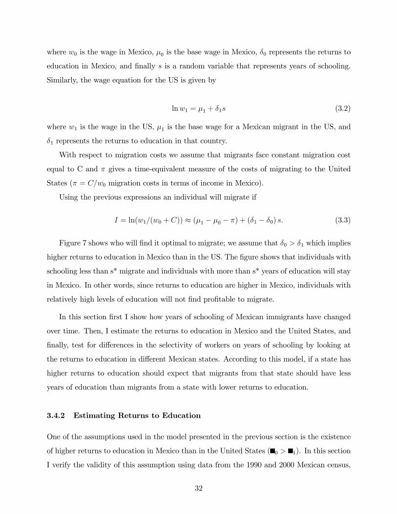
Figure 7 shows who will �nd it optimal to migrate; we assume that �0 > �1 which implies

higher returns to education in Mexico than in the US. The �gure shows that individuals with

schooling less than s* migrate and individuals with more than s* years of education will stay

in Mexico. In other words, since returns to education are higher in Mexico, individuals with

relatively high levels of education will not �nd pro�table to migrate.

In this section �rst I show how years of schooling of Mexican immigrants have changed

over time. Then, I estimate the returns to education in Mexico and the United States, and

�nally, test for di¤erences in the selectivity of workers on years of schooling by looking at

the returns to education in di¤erent Mexican states. According to this model, if a state has

higher returns to education should expect that migrants from that state should have less

years of education than migrants from a state with lower returns to education.

3.4.2 Estimating Returns to Education

One of the assumptions used in the model presented in the previous section is the existence

of higher returns to education in Mexico than in the United States ( 0 > 1). In this section

I verify the validity of this assumption using data from the 1990 and 2000 Mexican census,

32

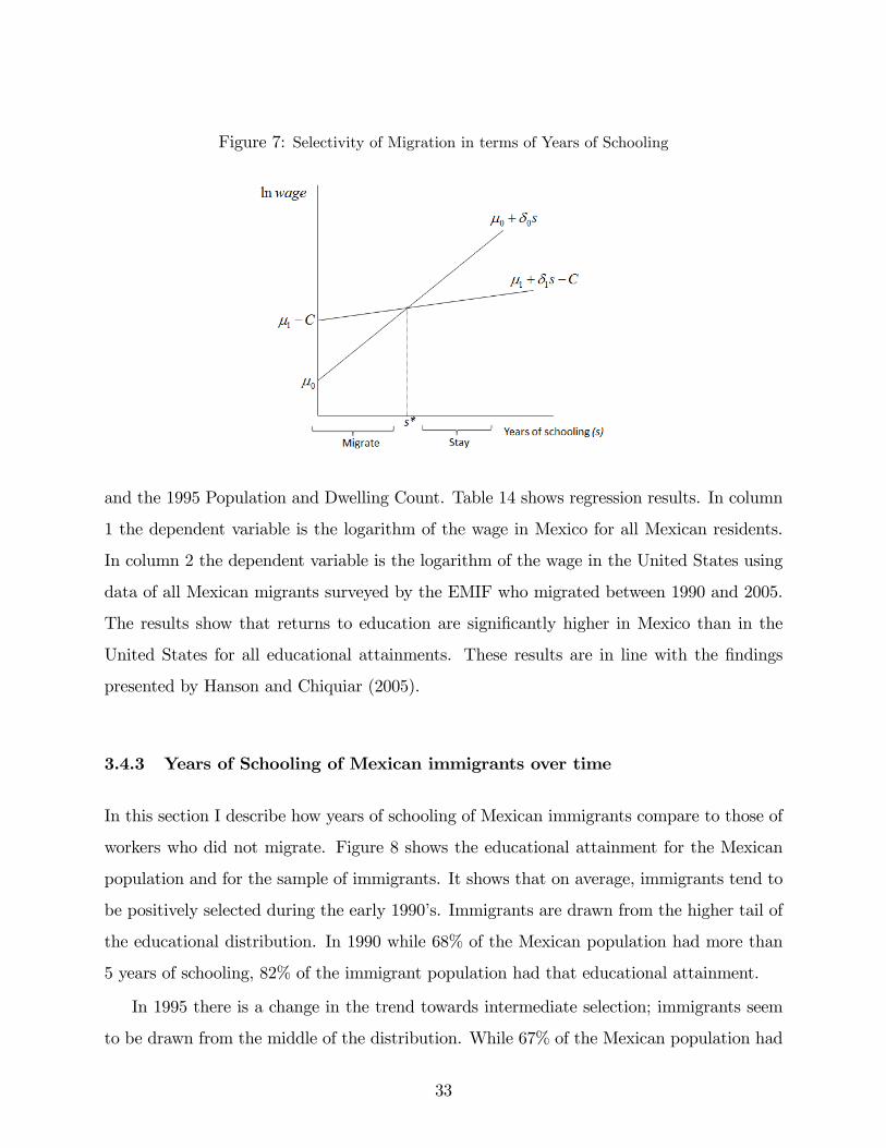
Figure 7: Selectivity of Migration in terms of Years of Schooling

and the 1995 Population and Dwelling Count. Table 14 shows regression results. In column

1 the dependent variable is the logarithm of the wage in Mexico for all Mexican residents.

In column 2 the dependent variable is the logarithm of the wage in the United States using

data of all Mexican migrants surveyed by the EMIF who migrated between 1990 and 2005.

The results show that returns to education are signi�cantly higher in Mexico than in the

United States for all educational attainments. These results are in line with the �ndings

presented by Hanson and Chiquiar (2005).

3.4.3 Years of Schooling of Mexican immigrants over time

In this section I describe how years of schooling of Mexican immigrants compare to those of

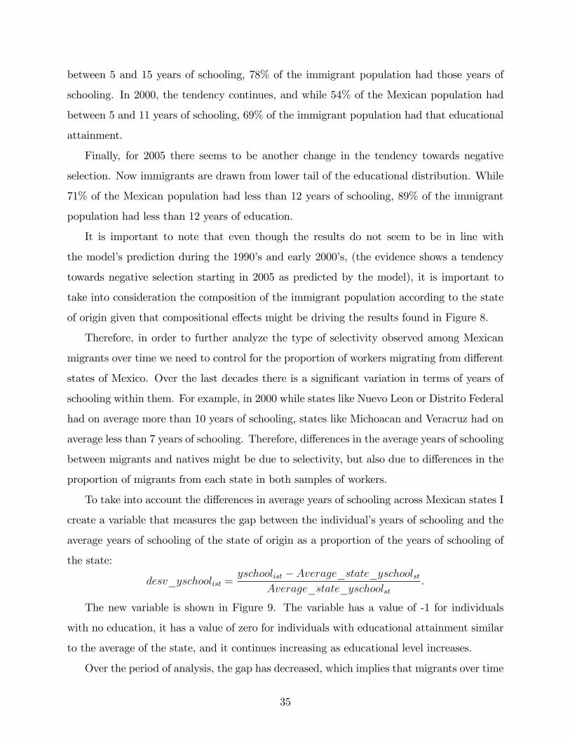
workers who did not migrate. Figure 8 shows the educational attainment for the Mexican

population and for the sample of immigrants. It shows that on average, immigrants tend to

be positively selected during the early 1990�s. Immigrants are drawn from the higher tail of

the educational distribution. In 1990 while 68% of the Mexican population had more than

5 years of schooling, 82% of the immigrant population had that educational attainment.

In 1995 there is a change in the trend towards intermediate selection; immigrants seem

to be drawn from the middle of the distribution. While 67% of the Mexican population had

33

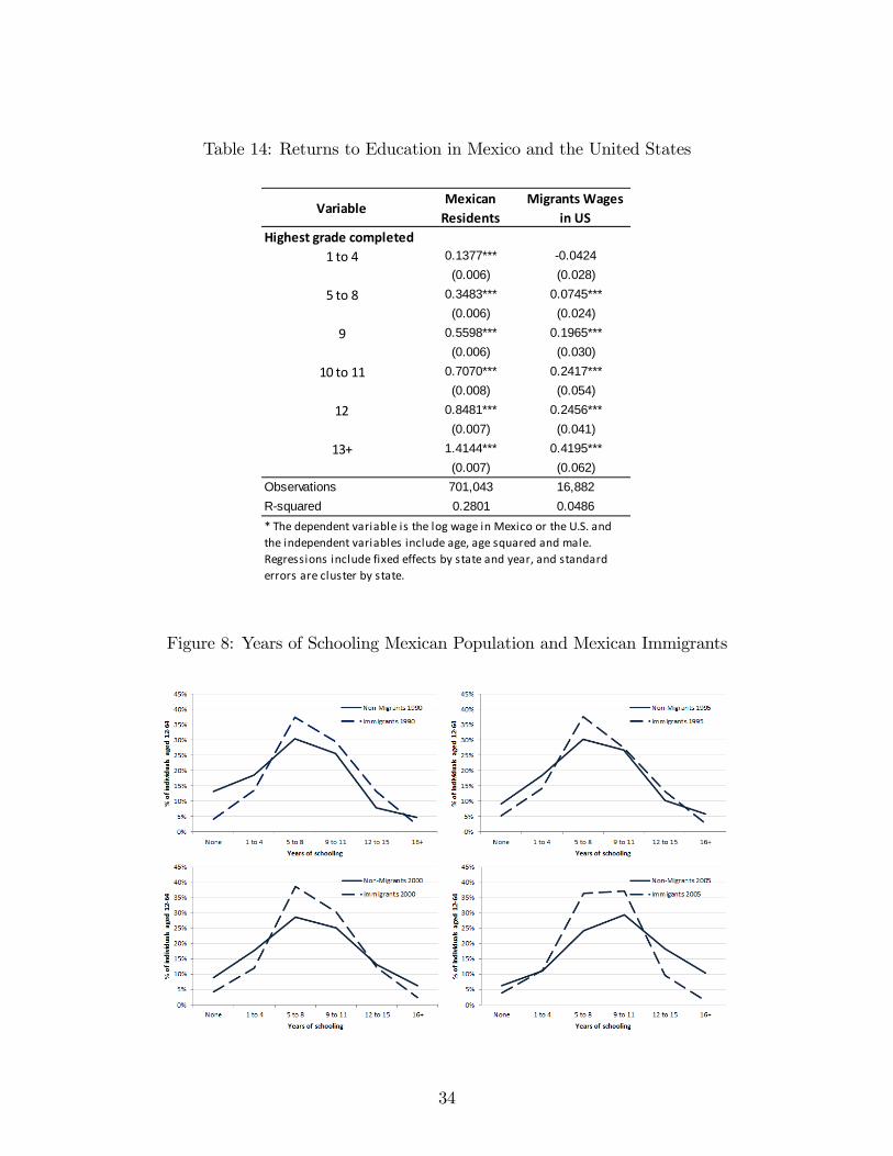
Table 14: Returns to Education in Mexico and the United States

VariableMexican

ResidentsMigrants Wages

in USHighest grade completed

1 to 4 0.1377*** ­0.0424(0.006) (0.028)

5 to 8 0.3483*** 0.0745***(0.006) (0.024)

9 0.5598*** 0.1965***(0.006) (0.030)

10 to 11 0.7070*** 0.2417***(0.008) (0.054)

12 0.8481*** 0.2456***(0.007) (0.041)

13+ 1.4144*** 0.4195***(0.007) (0.062)

Observations 701,043 16,882R­squared 0.2801 0.0486* The dependent variable is the log wage in Mexico or the U.S. andthe independent variables include age, age squared and male.Regressions include fixed effects by state and year, and standarderrors are cluster by state.

Figure 8: Years of Schooling Mexican Population and Mexican Immigrants

34

between 5 and 15 years of schooling, 78% of the immigrant population had those years of

schooling. In 2000, the tendency continues, and while 54% of the Mexican population had

between 5 and 11 years of schooling, 69% of the immigrant population had that educational

attainment.

Finally, for 2005 there seems to be another change in the tendency towards negative

selection. Now immigrants are drawn from lower tail of the educational distribution. While

71% of the Mexican population had less than 12 years of schooling, 89% of the immigrant

population had less than 12 years of education.

It is important to note that even though the results do not seem to be in line with

the model�s prediction during the 1990�s and early 2000�s, (the evidence shows a tendency

towards negative selection starting in 2005 as predicted by the model), it is important to

take into consideration the composition of the immigrant population according to the state

of origin given that compositional e¤ects might be driving the results found in Figure 8.

Therefore, in order to further analyze the type of selectivity observed among Mexican

migrants over time we need to control for the proportion of workers migrating from di¤erent

states of Mexico. Over the last decades there is a signi�cant variation in terms of years of

schooling within them. For example, in 2000 while states like Nuevo Leon or Distrito Federal

had on average more than 10 years of schooling, states like Michoacan and Veracruz had on

average less than 7 years of schooling. Therefore, di¤erences in the average years of schooling

between migrants and natives might be due to selectivity, but also due to di¤erences in the

proportion of migrants from each state in both samples of workers.

To take into account the di¤erences in average years of schooling across Mexican states I

create a variable that measures the gap between the individual�s years of schooling and the

average years of schooling of the state of origin as a proportion of the years of schooling of

the state:

desv_yschoolist =yschoolist � Average_state_yschoolst

Average_state_yschoolst:

The new variable is shown in Figure 9. The variable has a value of -1 for individuals

with no education, it has a value of zero for individuals with educational attainment similar

to the average of the state, and it continues increasing as educational level increases.

Over the period of analysis, the gap has decreased, which implies that migrants over time

35

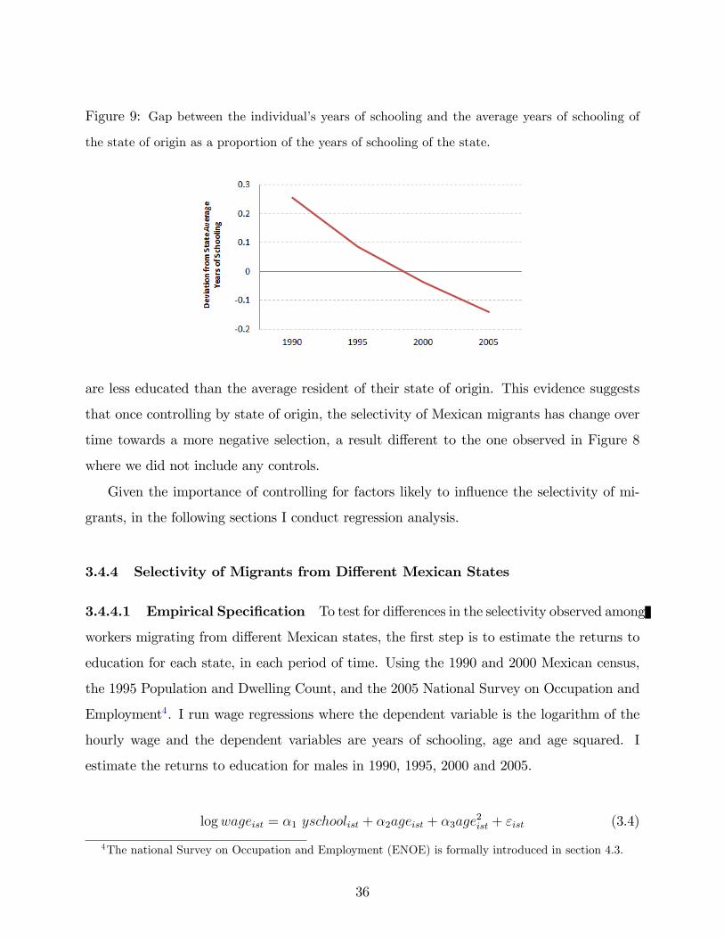
Figure 9: Gap between the individual�s years of schooling and the average years of schooling of

the state of origin as a proportion of the years of schooling of the state.

are less educated than the average resident of their state of origin. This evidence suggests

that once controlling by state of origin, the selectivity of Mexican migrants has change over

time towards a more negative selection, a result di¤erent to the one observed in Figure 8

where we did not include any controls.

Given the importance of controlling for factors likely to in�uence the selectivity of mi-

grants, in the following sections I conduct regression analysis.

3.4.4 Selectivity of Migrants from Di¤erent Mexican States

3.4.4.1 Empirical Speci�cation To test for di¤erences in the selectivity observed among

workers migrating from di¤erent Mexican states, the �rst step is to estimate the returns to

education for each state, in each period of time. Using the 1990 and 2000 Mexican census,

the 1995 Population and Dwelling Count, and the 2005 National Survey on Occupation and

Employment4. I run wage regressions where the dependent variable is the logarithm of the

hourly wage and the dependent variables are years of schooling, age and age squared. I

estimate the returns to education for males in 1990, 1995, 2000 and 2005.

logwageist = �1 yschoolist + �2ageist + �3age2ist + "ist (3.4)

4The national Survey on Occupation and Employment (ENOE) is formally introduced in section 4.3.

36

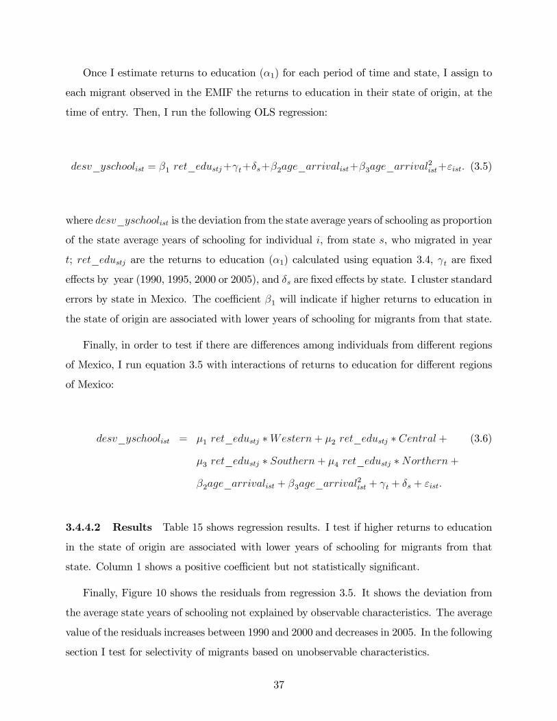
Once I estimate returns to education (�1) for each period of time and state, I assign to

each migrant observed in the EMIF the returns to education in their state of origin, at the

time of entry. Then, I run the following OLS regression:

desv_yschoolist = �1 ret_edustj+ t+�s+�2age_arrivalist+�3age_arrival2ist+"ist: (3.5)

where desv_yschoolist is the deviation from the state average years of schooling as proportion

of the state average years of schooling for individual i, from state s, who migrated in year

t; ret_edustj are the returns to education (�1) calculated using equation 3.4, t are �xed

e¤ects by year (1990, 1995, 2000 or 2005), and �s are �xed e¤ects by state. I cluster standard

errors by state in Mexico. The coe¢ cient �1 will indicate if higher returns to education in

the state of origin are associated with lower years of schooling for migrants from that state.

Finally, in order to test if there are di¤erences among individuals from di¤erent regions

of Mexico, I run equation 3.5 with interactions of returns to education for di¤erent regions

of Mexico:

desv_yschoolist = �1 ret_edustj �Western+ �2 ret_edustj � Central + (3.6)

�3 ret_edustj � Southern+ �4 ret_edustj �Northern+

�2age_arrivalist + �3age_arrival2ist + t + �s + "ist:

3.4.4.2 Results Table 15 shows regression results. I test if higher returns to education

in the state of origin are associated with lower years of schooling for migrants from that

state. Column 1 shows a positive coe¢ cient but not statistically signi�cant.

Finally, Figure 10 shows the residuals from regression 3.5. It shows the deviation from

the average state years of schooling not explained by observable characteristics. The average

value of the residuals increases between 1990 and 2000 and decreases in 2005. In the following

section I test for selectivity of migrants based on unobservable characteristics.

37

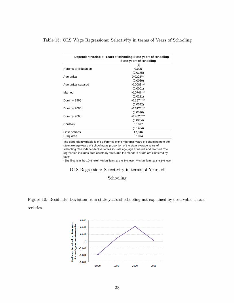
Table 15: OLS Wage Regressions: Selectivity in terms of Years of Schooling

Dependent variable: Years of schooling­State years of schoolingState years of schooling

(1)Returns to Education 0.005

(0.0175)Age arrival 0.0208***

(0.0039)Age arrival squared ­0.0005***

(0.0001)Married ­0.0747***

(0.0221)Dummy 1995 ­0.1874***

(0.0342)Dummy 2000 ­0.3125***

(0.0316)Dummy 2005 ­0.4025***

(0.0284)Constant 0.1077

(0.1494)Observations 17,946R­squared 0.1074

*Significant at the 10% level, **significant at the 5% level, ***significant at the 1% level.

The dependent variable is the difference of the migrant's years of schooling from thestate average years of schooling as proportion of the state average years ofschooling. The independent variables include age, age squared, and married. Theregression includes fixed effects by state, and the standard errors are clustered bystate.

OLS Regression: Selectivity in terms of Years of

Schooling

Figure 10: Residuals: Deviation from state years of schooling not explained by observable charac-

teristics

38

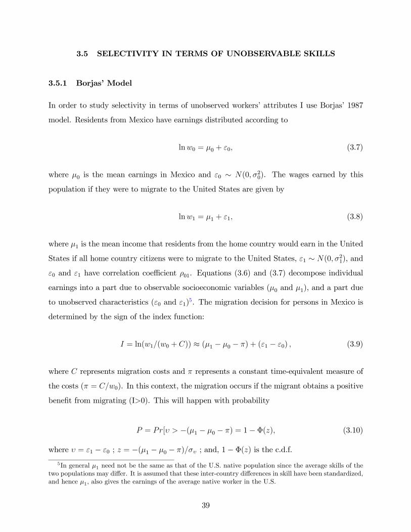
3.5 SELECTIVITY IN TERMS OF UNOBSERVABLE SKILLS

3.5.1 Borjas�Model

In order to study selectivity in terms of unobserved workers�attributes I use Borjas�1987

model. Residents from Mexico have earnings distributed according to

lnw0 = �0 + "0; (3.7)

where �0 is the mean earnings in Mexico and "0 � N(0; �20). The wages earned by this

population if they were to migrate to the United States are given by

lnw1 = �1 + "1; (3.8)

where �1 is the mean income that residents from the home country would earn in the United

States if all home country citizens were to migrate to the United States, "1 � N(0; �21), and

"0 and "1 have correlation coe¢ cient �01. Equations (3.6) and (3.7) decompose individual

earnings into a part due to observable socioeconomic variables (�0 and �1), and a part due

to unobserved characteristics ("0 and "1)5. The migration decision for persons in Mexico is

determined by the sign of the index function:

I = ln(w1=(w0 + C)) � (�1 � �0 � �) + ("1 � "0) ; (3.9)

where C represents migration costs and � represents a constant time-equivalent measure of

the costs (� = C=w0). In this context, the migration occurs if the migrant obtains a positive

bene�t from migrating (I>0). This will happen with probability

P = Pr[� > �(�1 � �0 � �) = 1� �(z); (3.10)

where � = "1 � "0 ; z = �(�1 � �0 � �)=�� ; and, 1� �(z) is the c.d.f.5In general �1 need not be the same as that of the U.S. native population since the average skills of the

two populations may di¤er. It is assumed that these inter-country di¤erences in skill have been standardized,and hence �1, also gives the earnings of the average native worker in the U.S.

39

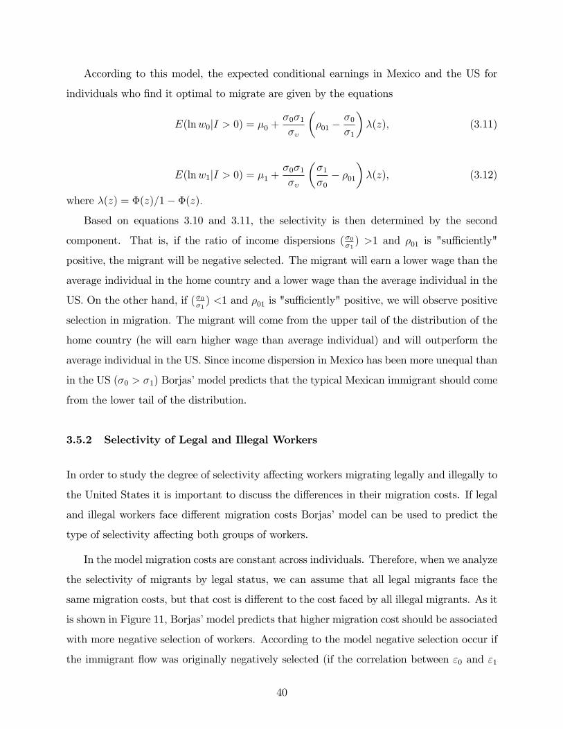
According to this model, the expected conditional earnings in Mexico and the US for

individuals who �nd it optimal to migrate are given by the equations

E(lnw0jI > 0) = �0 +�0�1��

��01 �

�0�1

��(z); (3.11)

E(lnw1jI > 0) = �1 +�0�1��

��1�0� �01

��(z); (3.12)

where �(z) = �(z)=1� �(z):

Based on equations 3.10 and 3.11, the selectivity is then determined by the second

component. That is, if the ratio of income dispersions (�0�1) >1 and �01 is "su¢ ciently"

positive, the migrant will be negative selected. The migrant will earn a lower wage than the

average individual in the home country and a lower wage than the average individual in the

US. On the other hand, if (�0�1) <1 and �01 is "su¢ ciently" positive, we will observe positive

selection in migration. The migrant will come from the upper tail of the distribution of the

home country (he will earn higher wage than average individual) and will outperform the

average individual in the US. Since income dispersion in Mexico has been more unequal than

in the US (�0 > �1) Borjas�model predicts that the typical Mexican immigrant should come

from the lower tail of the distribution.

3.5.2 Selectivity of Legal and Illegal Workers

In order to study the degree of selectivity a¤ecting workers migrating legally and illegally to

the United States it is important to discuss the di¤erences in their migration costs. If legal

and illegal workers face di¤erent migration costs Borjas�model can be used to predict the

type of selectivity a¤ecting both groups of workers.

In the model migration costs are constant across individuals. Therefore, when we analyze

the selectivity of migrants by legal status, we can assume that all legal migrants face the

same migration costs, but that cost is di¤erent to the cost faced by all illegal migrants. As it

is shown in Figure 11, Borjas�model predicts that higher migration cost should be associated

with more negative selection of workers. According to the model negative selection occur if

the immigrant �ow was originally negatively selected (if the correlation between "0 and "1

40

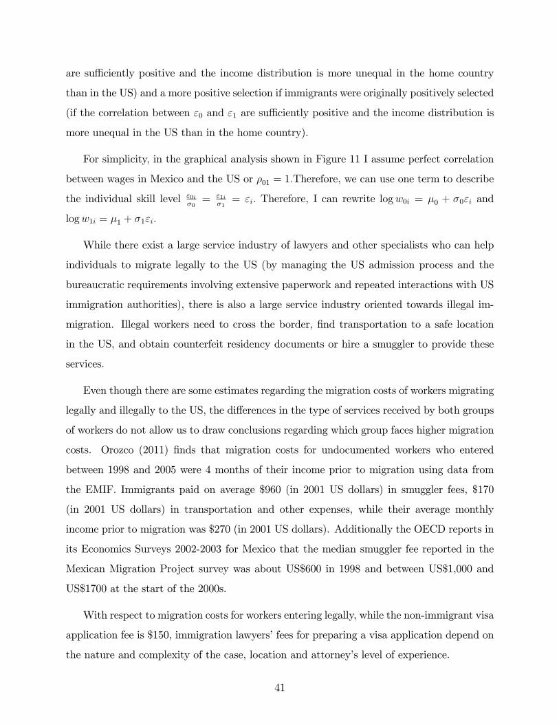
are su¢ ciently positive and the income distribution is more unequal in the home country

than in the US) and a more positive selection if immigrants were originally positively selected

(if the correlation between "0 and "1 are su¢ ciently positive and the income distribution is

more unequal in the US than in the home country).

For simplicity, in the graphical analysis shown in Figure 11 I assume perfect correlation

between wages in Mexico and the US or �01 = 1:Therefore, we can use one term to describe

the individual skill level "0i�0= "1i

�1= "i: Therefore, I can rewrite logw0i = �0 + �0"i and

logw1i = �1 + �1"i:

While there exist a large service industry of lawyers and other specialists who can help

individuals to migrate legally to the US (by managing the US admission process and the

bureaucratic requirements involving extensive paperwork and repeated interactions with US

immigration authorities), there is also a large service industry oriented towards illegal im-

migration. Illegal workers need to cross the border, �nd transportation to a safe location

in the US, and obtain counterfeit residency documents or hire a smuggler to provide these

services.

Even though there are some estimates regarding the migration costs of workers migrating

legally and illegally to the US, the di¤erences in the type of services received by both groups

of workers do not allow us to draw conclusions regarding which group faces higher migration

costs. Orozco (2011) �nds that migration costs for undocumented workers who entered

between 1998 and 2005 were 4 months of their income prior to migration using data from

the EMIF. Immigrants paid on average $960 (in 2001 US dollars) in smuggler fees, $170

(in 2001 US dollars) in transportation and other expenses, while their average monthly

income prior to migration was $270 (in 2001 US dollars). Additionally the OECD reports in

its Economics Surveys 2002-2003 for Mexico that the median smuggler fee reported in the

Mexican Migration Project survey was about US$600 in 1998 and between US$1,000 and

US$1700 at the start of the 2000s.

With respect to migration costs for workers entering legally, while the non-immigrant visa

application fee is $150, immigration lawyers�fees for preparing a visa application depend on

the nature and complexity of the case, location and attorney�s level of experience.

41

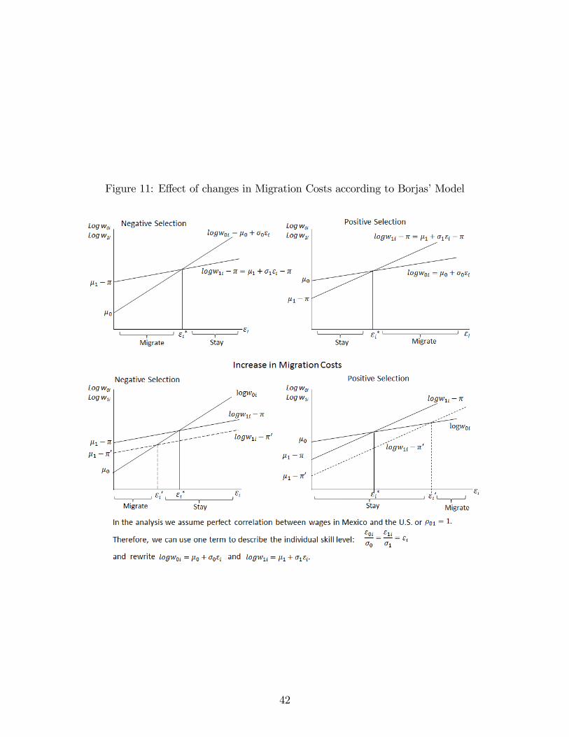
Figure 11: E¤ect of changes in Migration Costs according to Borjas�Model

42

If we assume that migration costs are higher for illegal workers Borjas�model would pre-

dict a more negative selection among that group of workers if they were originally negatively

selected; and a more positive selection among that group of migrants if they are originally

positively selected. In the next sections I will test if Borjas�predictions relative to the type of

selectivity observed among legal and illegal workers are supported by the empirical evidence.

3.5.3 Empirical Speci�cation

According to Borjas�model, the average earnings of immigrants can be written as

E(lnw0jI > 0) = �0 + ��0�1��

��� �0

�1

�;

which implies that an increase in income inequality represented as an increase in the ratio

of variances of the income distribution in Mexico relative to that in the United States��0�1

�should worsen the earnings of those migrants who �nd it optimal to migrate to the United

States with respect to the earnings of non-immigrants in Mexico with the same observable

characteristics.

In order to test how income inequality impacts the degree of selectivity of Mexican

immigrants I exploit the variation of income inequality in di¤erent states of Mexico over

time using OLS regressions.

The �rst step is to predict the wage that the worker could have earned in Mexico if he

had not migrated from state s in period t based on his observable characteristics. I estimate

OLS regressions using Mexican census data and the 1995 Population and Dwelling Count.

The dependent variable is the logarithm of the hourly wage and the independent variables

are years of schooling, age of arrival, age of arrival squared, experience prior to migration, ex-

perience prior to migration squared, and interactions between years of education, experience

and age.

lnwageMexist = �1yschoolist + �2ageist + �3age

2ist + �4experienceist + �5experience

2ist

+�6yschoolist � ageist + �7yschoolist � experienceist (3.13)

+�8experienceist � ageist + "ist

43

The coe¢ cients obtained in regression 3.12 will be used to estimate the wages that

migrants surveyed by the EMIF would have earned if they had not migrated. Using �1 �

�8 and the migrants� characteristics, I estimate \lnwageMexist : In order to predict workers�

wages individuals were grouped by year of arrival into 3 categories. For individuals who

migrated between 1990 and 1992 predicted wages were estimated the �0s obtained from

running regression 3.12 using census data from 1990, for those who entered between 1993

and 1997 the �0s obtained using data from the 1995 Population and Dwelling Count was

used, and �nally, for those who entered between 1998 and 2005 the �0s used to predict

their wages are estimated using the 2000 Mexican census. I predict the wages of immigrants

surveyed by the EMIF who migrated to the United States between 1990 and 2003 who were

surveyed within the �rst 3 years after entering the US, who were working in Mexico prior to

migration and reported their wages.

Then I estimate the portion of the wage in Mexico associated with workers�unobservable

characteristics (the di¤erence between the logarithm of the real hourly wage of individual

i; who migrated from state s at time t; and the logarithm of the predicted wage that the

worker could have earned in Mexico if he had not migrated from state s in period t).

unobservableMexist = (lnwageMex

ist � \lnwageMexist )

The next step is to run an OLS regression (Model 1) where the dependent variable is

the portion of the wage in Mexico associated with workers�unobservable characteristics. As

independent variables I include the ratio of the Gini coe¢ cient for the Mexican state s at

time t; to the Gini coe¢ cient for the United States at time t6. Additionally, since social

networks are an important factor likely to in�uence the type of selectivity observed among

immigrants, I include the size of the immigrant network in the United States for workers

from di¤erent states of origin (proxied by the number of the immigrants who migrated in

the previous �ve years as a proportion of the current population of each Mexican state).

6I use the Gini coe¢ cient for the United States (not by state) because when individuals make the decisionto migrate they have a general idea of the prevailing economic conditions in the United States, and anexpectation of the wages they could earned, but not very detailed information about the state where theywill end up working. Moreover, the EMIF reports the state of the US where immigrants were working at thetime of the survey, but not the �rst state where they worked after migrating. As a future extension, Ginicoe¢ cients by state in the US will be included.

44

Finally, I include migration costs (proxied by the distance from the capital of the state

of origin in Mexico to the state of destination in the United States), and the logarithm of

the state GDP per capita. The regression includes controls for state of residence in Mexico

prior to migration, year of migration, duration in the US at the time of the survey, and the

number of years passed between the year of migration and the year of the Census used to

predict the worker�s wage \(lnwageMexist ): Additionally, I cluster standard errors by state of

residence in Mexico and include sample weights.

I estimate this regression using data of immigrants who migrated to the United States

between 1990 and 2003 who were surveyed within the �rst 3 years after entering the US,

who were working in Mexico prior to migration and reported their wages. Additionally, I

restrict the sample to include males who were born in Mexico, aged 12 to 64 at the time

of migration, and eliminate 0.05% of the observations with the highest and lowest hourly

wages.

unobservableMexist = �1gini

Mexst =giniUSt + �2networksst

+�3migration_costsist (3.14)

+�4 ln gdp_percapitast + "ist

In order to test for di¤erences in the selectivity of individuals migrating legally and

illegally to the US, Model 2 includes the regressors included in Model 1 plus a dummy

variable for workers who migrated legally to the US and an interaction of the ratio of the

Gini coe¢ cients between Mexico and the United States and the dummy variable for legal

status at the time of entry.

unobservableMexist = �1gini

Mexst =giniUSt + �2gini

Mexst =giniUSt � legal_entry (3.15)

+�3legal_entryist + �4networksst + �5migration_costsist

+�6 ln gdp_percapitast + "ist

Next, in order to test for di¤erences in the selectivity of workers based on their observ-

able characteristics I run an OLS regression (Model 3) where the dependent variable is the

logarithm of the predicted wage that the worker could have earned in Mexico if he had

45

not migrated from state s in period t. The independent variables and the controls used

are the ones included in Model 1. I cluster standard errors by state of residence in Mexico

and include sample weights. Additionally, I test for di¤erences in the type of selectivity of

workers by legal status. Model 4 includes the regressors included in Model 3 plus a dummy

variable for workers who migrated legally to the US and an interaction of the ratio of the

Gini coe¢ cients between Mexico and the United States and the dummy variable for legal

status at the time of entry.

observableMexist = \lnwageist = �1giniMex

st =giniUSt + �2networksst

+�3migration_costsist + �4 ln gdp_percapitast + "ist (3.16)

observableMexist = �1gini

Mexst =giniUSt + �2gini

Mexst =giniUSt � legal_entryist

+�3legal_entryist + �4networksst + �5migration_costsist

+�6 ln gdp_percapitast + "ist (3.17)

It is important to note that the immigration phenomenon, and the selectivity observed

among those immigrants can potentially a¤ect the degree of income inequality in Mexican

states, especially in the long run. If immigrants are drawn from the lower tail of the income

distribution, their migration decision could have a positive e¤ect on the income distribution

(decreasing income inequality) of their state of origin. Previous literature studying the e¤ect

of migration on inequality has focused on the e¤ect of remittances. Their �ndings show that

remittances decrease income inequality and poverty especially when they are used for in-

vestment purposes (Taylor, Mora, Adams, and Lopez-Feldman 2005, Taylor 1999, Adelman

and Taylor 1990). If this were the case, the results could be potentially biased due to a

problem of reverse causality. However, given that a more negative selection of immigrants

can potentially be correlated with a decrease in income inequality, my estimates could be

underestimating the true e¤ect but could be interpreted as a lower bound. Fortunately, there

is no evidence that this empirical speci�cation is a¤ected by reverse causality. Individuals

make the decision to migrate when they look at the current economic conditions (current

46

income inequality). Even though their decision to migrate can potentially impact the income

inequality that will be faced by individuals next period, the evidence shows that changes

in the selectivity a¤ecting immigrants is not a determinant factor of the degree of inequal-

ity observed in Mexican states. This results suggest that remittances are used mainly for

consumption purposes and do not a¤ect the income inequality in sending regions.7.

Finally, I analyze the e¤ect of changes in income inequality but using the wages of workers

in the United States, an exercise similar to Borjas�empirical analysis. The �rst step is to

predict the wage that workers were earning in the United States one year after migration

based on their observable characteristics and their legal status. I estimate an OLS regression

using data of earnings in the United States of male workers surveyed by the EMIF between

1993 and 2005, who were born in Mexico, aged 12 to 64 at the time of migration, aged 12

to 64 at the time of the survey, who worked in the United States at least one month and

reported their earnings.

The dependent variable is the logarithm of the hourly wage in the US of worker i, who

migrated from state s; and that is surveyed by the EMIF at time T , and the independent

variables are years of schooling, age, age squared, experience in the United States (calculated

as the di¤erence between the year of migration and the year in which the survey was con-

ducted), experience squared, interactions between years of education, experience and age, a

dummy variable for legal status, and controls by the calendar year of migration.

lnwageUSisT = �1yschoolisT + �2ageisT + �3age2isT + �4experience_USisT (3.18)

+�5experience_US2isT + �6yschoolisT � age

+�7yschoolisT � experience_USisT

+�8experienceisT � age+ �9year_entryisT + "isT

I use the coe¢ cients (�0s) of regression 3.17 to calculate the predicted wages of workers�\lnwageUSist+1

�with one year of experience in the United States (at t+1) who entered legally

and illegally to the United States.7The evidence shows that shortly after migration, remittances are more likely to be used to repay loans

and consumption expenditures rather than for investment purposes. This phenomenon could explain whywe do not observe an e¤ect on income inequality in the short run.

47

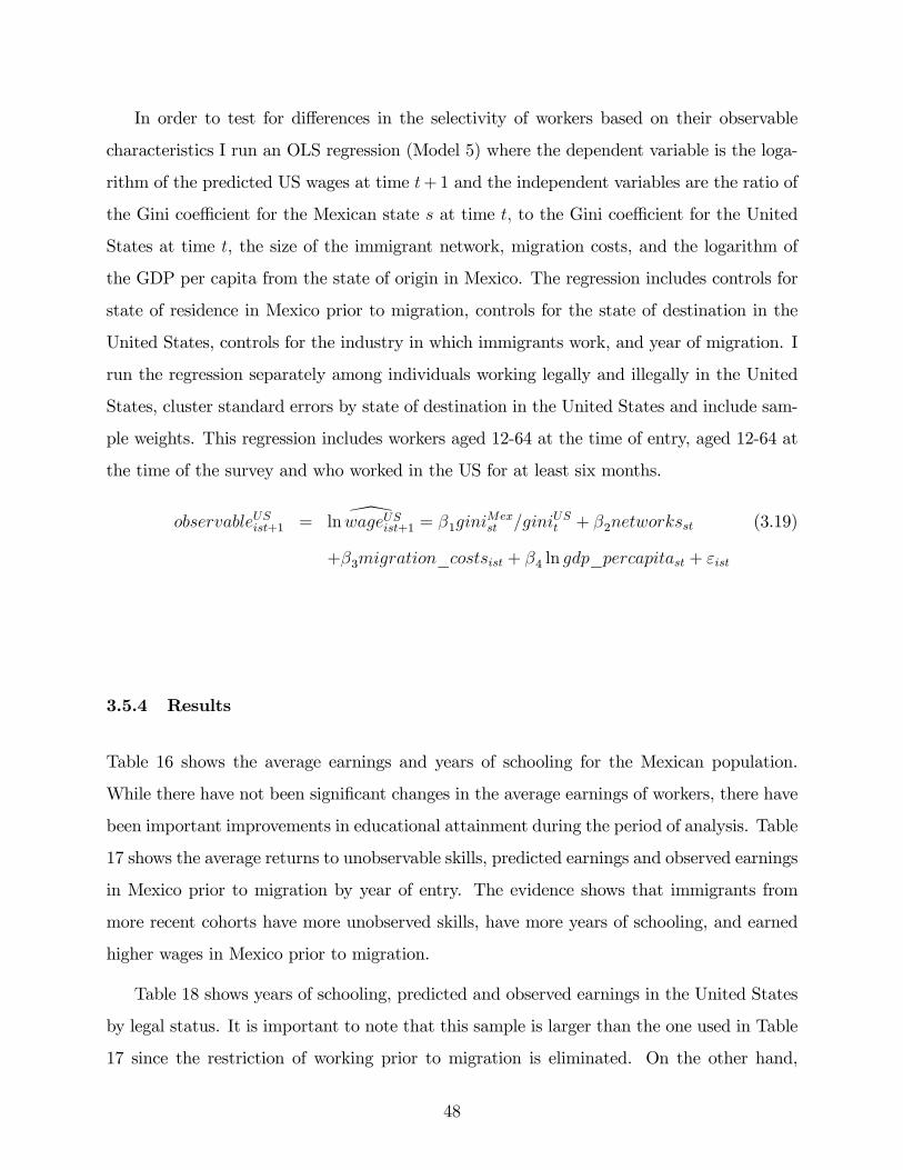
In order to test for di¤erences in the selectivity of workers based on their observable

characteristics I run an OLS regression (Model 5) where the dependent variable is the loga-

rithm of the predicted US wages at time t+1 and the independent variables are the ratio of

the Gini coe¢ cient for the Mexican state s at time t; to the Gini coe¢ cient for the United

States at time t, the size of the immigrant network, migration costs, and the logarithm of

the GDP per capita from the state of origin in Mexico. The regression includes controls for

state of residence in Mexico prior to migration, controls for the state of destination in the

United States, controls for the industry in which immigrants work, and year of migration. I

run the regression separately among individuals working legally and illegally in the United

States, cluster standard errors by state of destination in the United States and include sam-

ple weights. This regression includes workers aged 12-64 at the time of entry, aged 12-64 at

the time of the survey and who worked in the US for at least six months.

observableUSist+1 = \lnwageUSist+1 = �1giniMexst =giniUSt + �2networksst (3.19)

+�3migration_costsist + �4 ln gdp_percapitast + "ist

3.5.4 Results

Table 16 shows the average earnings and years of schooling for the Mexican population.

While there have not been signi�cant changes in the average earnings of workers, there have

been important improvements in educational attainment during the period of analysis. Table

17 shows the average returns to unobservable skills, predicted earnings and observed earnings

in Mexico prior to migration by year of entry. The evidence shows that immigrants from

more recent cohorts have more unobserved skills, have more years of schooling, and earned

higher wages in Mexico prior to migration.

Table 18 shows years of schooling, predicted and observed earnings in the United States

by legal status. It is important to note that this sample is larger than the one used in Table

17 since the restriction of working prior to migration is eliminated. On the other hand,

48

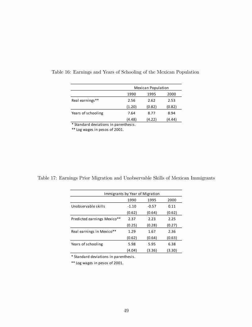
Table 16: Earnings and Years of Schooling of the Mexican Population

1990 1995 2000Real earnings** 2.56 2.62 2.53

(1.20) (0.82) (0.82)Years of schooling 7.64 8.77 8.94

(4.48) (4.22) (4.44)* Standard deviations in parenthesis.** Log wages in pesos of 2001.

Mexican Population

Table 17: Earnings Prior Migration and Unobservable Skills of Mexican Immigrants

Immigrants by Year of Migration1990 1995 2000

Unobservable skil ls ­1.10 ­0.57 0.11(0.62) (0.64) (0.62)

Predicted earnings Mexico** 2.37 2.23 2.25(0.25) (0.28) (0.27)

Real earnings in Mexico** 1.29 1.67 2.36(0.62) (0.64) (0.63)

Years of schooling 5.98 5.95 6.38(4.04) (3.36) (3.30)

* Standard deviations in parenthesis.** Log wages in pesos of 2001.

49

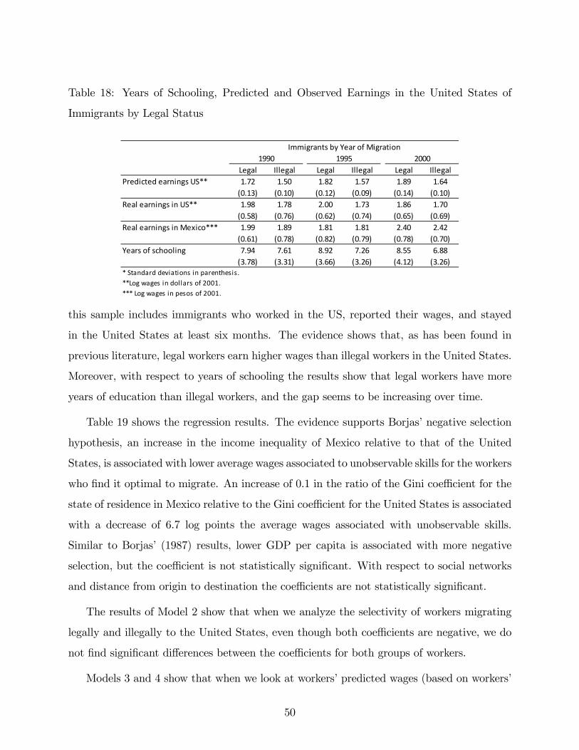
Table 18: Years of Schooling, Predicted and Observed Earnings in the United States of

Immigrants by Legal Status

Legal Illegal Legal Illegal Legal IllegalPredicted earnings US** 1.72 1.50 1.82 1.57 1.89 1.64

(0.13) (0.10) (0.12) (0.09) (0.14) (0.10)Real earnings in US** 1.98 1.78 2.00 1.73 1.86 1.70

(0.58) (0.76) (0.62) (0.74) (0.65) (0.69)Real earnings in Mexico*** 1.99 1.89 1.81 1.81 2.40 2.42

(0.61) (0.78) (0.82) (0.79) (0.78) (0.70)Years of schooling 7.94 7.61 8.92 7.26 8.55 6.88

(3.78) (3.31) (3.66) (3.26) (4.12) (3.26)* Standard deviations in parenthesis.**Log wages in dollars of 2001.*** Log wages in pesos of 2001.

Immigrants by Year of Migration1990 1995 2000

this sample includes immigrants who worked in the US, reported their wages, and stayed

in the United States at least six months. The evidence shows that, as has been found in

previous literature, legal workers earn higher wages than illegal workers in the United States.

Moreover, with respect to years of schooling the results show that legal workers have more

years of education than illegal workers, and the gap seems to be increasing over time.

Table 19 shows the regression results. The evidence supports Borjas�negative selection

hypothesis, an increase in the income inequality of Mexico relative to that of the United

States, is associated with lower average wages associated to unobservable skills for the workers

who �nd it optimal to migrate. An increase of 0.1 in the ratio of the Gini coe¢ cient for the

state of residence in Mexico relative to the Gini coe¢ cient for the United States is associated

with a decrease of 6.7 log points the average wages associated with unobservable skills.

Similar to Borjas� (1987) results, lower GDP per capita is associated with more negative

selection, but the coe¢ cient is not statistically signi�cant. With respect to social networks

and distance from origin to destination the coe¢ cients are not statistically signi�cant.

The results of Model 2 show that when we analyze the selectivity of workers migrating

legally and illegally to the United States, even though both coe¢ cients are negative, we do

not �nd signi�cant di¤erences between the coe¢ cients for both groups of workers.

Models 3 and 4 show that when we look at workers�predicted wages (based on workers�

50

Table 19: E¤ect of Changes in Income Inequality on the Selectivity of Mexican Migrants

using Earnings Prior Migration

Gini Mex/Gini US ­0.675 ** ­0.268(0.306) (0.209)

Gini Mex/Gini US*Legal ­1.038 ­0.308(0.713) (0.258)

Gini Mex/Gini US*Il lega l ­0.588 ** ­0.261(0.287) (0.210)

Legal  at entry 0.394 0.153(0.734) (0.115)

Age

Age squared

Per Capita  GDP 0.053 0.096 0.633 *** 0.602 ***(0.530) (0.534) (0.164) (0.159)

Distance 0.018 0.020 0.001 ­0.001(0.028) (0.029) (0.009) (0.009)

Network ­0.032 ­0.030 0.010 0.008(0.019) (0.019) (0.012) (0.011)

Constant ­263.6 *** ­261.6 *** 35.47 *** 34.04 ***(27.428) (28.097) (9.162) (9.459)

Observations 4,321 4,321 4,321 4,321Adj R­squared 0.2741 0.2754 0.4178 0.4335Includes  fixed effects  by s tate and year. Standard errors  are clustered by s tate.

Model  1 Model  2 Model  3 Model  4Unobservable ski l l s Observable ski l l s

51

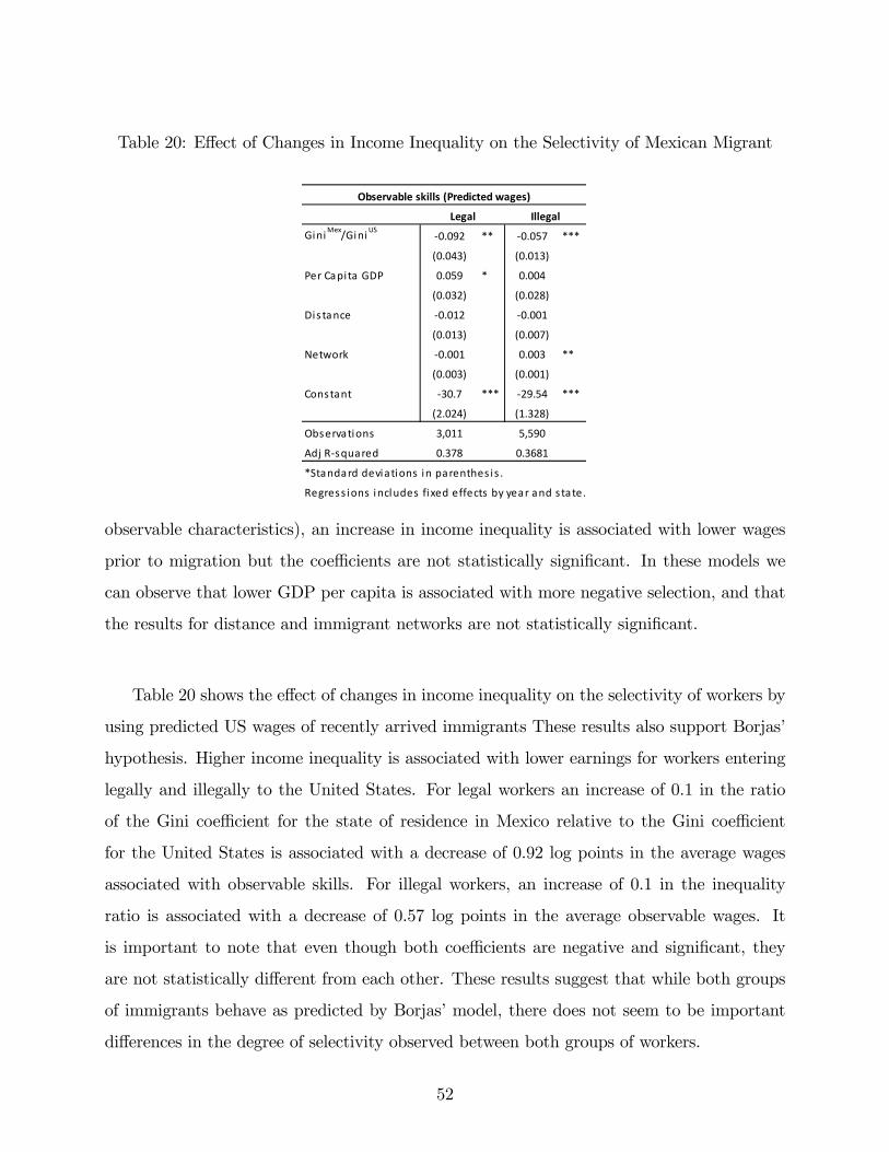
Table 20: E¤ect of Changes in Income Inequality on the Selectivity of Mexican Migrant

Gini Mex/Gini US­0.092 ** ­0.057 ***

(0.043) (0.013)

Per Capi ta  GDP 0.059 * 0.004

(0.032) (0.028)

Dis tance ­0.012 ­0.001

(0.013) (0.007)

Network ­0.001 0.003 **

(0.003) (0.001)

Constant ­30.7 *** ­29.54 ***

(2.024) (1.328)

Observations 3,011 5,590

Adj R­squared 0.378 0.3681

*Standard deviations  in parenthes is .

Regress ions  includes  fi xed effects  by year and s tate.

Observable skills (Predicted wages)

Legal Illegal

observable characteristics), an increase in income inequality is associated with lower wages

prior to migration but the coe¢ cients are not statistically signi�cant. In these models we

can observe that lower GDP per capita is associated with more negative selection, and that

the results for distance and immigrant networks are not statistically signi�cant.

Table 20 shows the e¤ect of changes in income inequality on the selectivity of workers by

using predicted US wages of recently arrived immigrants These results also support Borjas�

hypothesis. Higher income inequality is associated with lower earnings for workers entering

legally and illegally to the United States. For legal workers an increase of 0.1 in the ratio

of the Gini coe¢ cient for the state of residence in Mexico relative to the Gini coe¢ cient

for the United States is associated with a decrease of 0.92 log points in the average wages

associated with observable skills. For illegal workers, an increase of 0.1 in the inequality

ratio is associated with a decrease of 0.57 log points in the average observable wages. It

is important to note that even though both coe¢ cients are negative and signi�cant, they

are not statistically di¤erent from each other. These results suggest that while both groups

of immigrants behave as predicted by Borjas�model, there does not seem to be important

di¤erences in the degree of selectivity observed between both groups of workers.

52

With respect to social networks I �nd that for the coe¢ cient is not statistically signi�cant

for legal workers but is positive and signi�cant for illegal workers. While larger migration

networks have been previously associated with lower migration costs, especially among illegal

workers, larger social networks have also been associated with better labor market outcomes

of Mexican, especially among illegal workers. Finally, with respect to the GDP per capita

from state of origin I �nd positive coe¢ cients. Lower GDP per capita is associated with more

negative selection for both groups of workers, a result in line with the �ndings of Borjas 1987

and Jasso and Rosenzweig 1990.

3.6 CONCLUSIONS

In this paper I test Borjas�1987 negative selection hypothesis which states that individuals

migrating from states with more unequal income distributions and higher returns to skills

will be more negatively selected. I exploit the variation in returns to education and income

inequality across states in Mexico and over time to test for di¤erences in the type of selectivity

observed among legal and illegal immigrants. First, I analyze the selectivity in terms of years

of schooling. Then, using Borjas�selection model I infer worker�s unobservable skills by using

data of earnings prior to migration and analyze the degree of selectivity based on observable

and unobservable skills. Additionally, and following Borjas�1987 empirical speci�cation, I

predict the US wages of recently arrived immigrants to test for di¤erences in the degree of

selectivity observed among Mexican workers. I control for migration costs and the size of

immigrants�social networks, two important factors likely to in�uence immigrants�selectivity.

I use data of Mexican immigrants from the Survey of Migration to the Northern Border

(EMIF). Among the advantages of using this survey are that it provides information of

earnings prior to migration and earnings in the United States; identi�es workers by legal

status, and is conducted among workers temporarily and permanently settled in the United

States which allows me to account for return migration.

When I study years of education, while aggregate analysis �nd evidence of positive, inter-

mediate and negative selection in di¤erent periods of time, once we control for compositional

53

e¤ects we �nd evidence of negative selection of Mexican migrants at the state and region

level over the period of analysis. When I study the selectivity of workers using earnings prior

to migration I �nd that an increase in the income inequality of Mexico relative to that of

the United States, is associated with lower wages associated to unobservable skills for the

individuals who migrate to the United States.

Moreover, when I study the selectivity of workers using earnings in the United States

the evidence is also in line with Borjas�predictions. An increase in the income inequality of

Mexico relative to that of the United States is associated with lower wages associated with

observable skills for the workers who migrate legally and illegally to the United States. Even

though the results show that both groups of workers behave according to Borjas�hypothesis,

the evidence shows that there are not signi�cant di¤erences in the degree of selectivity

a¤ecting both groups of workers.

54

4.0 RETURN MIGRATION AND SELF-EMPLOYMENT IN MEXICO

4.1 MOTIVATION

Over the last four decades, Mexican households perceived immigration, whether temporary

or permanent, to be an e¤ective strategy for sustaining and improving their economic likeli-

hoods. On average, between 2001 and 2010, total remittances accounted for over $20 billion

dollars, representing one of the largest sources of foreign income in Mexico.

One channel through which migration may reduce poverty and promote growth is by en-

hancing the asset positions and productivity levels of poor households, either via remittances

and savings, or human capital accumulation. Households often face signi�cant production

constraints due to absent or incomplete credit markets. Remittances and savings from work

abroad, thus, may enable individuals to set up their own business upon return overcoming

liquidity constraints, low initial endowments or imperfect credit markets. In addition, the

skills acquired by migrants in the host countries may be put to productive use upon return.

The empirical literature studying the e¤ect of return migration on the probability of self-

employment has shown mixed results. While some studies have found evidence that return

migration contributed to the relaxation of credit constraints, fostering productive investment

(Woodru¤ et al., (2004); Dustmann et al., (2002); Murphy, (2000)), others have found that

remittances and savings are mainly used for consumption and non-productive investment

having no impact on investment, development and growth (King et al., (2003); Kule et al.,

(2002); Carletto et al., (2004); Germenji et al., (2004)).

In this chapter I assess the impact of return migration on self-employment exploiting

the variation in return migration rates to di¤erent states of Mexico in two di¤erent periods

55

of time. I predict return migration to di¤erent Mexican states by using past migration

patterns and use these predicted rates as instruments for return migration avoiding potential

endogeneity issues.

Di¤erent to what has been done in the literature, I study the e¤ect of return migration,

not only remittances, on self-employment. I exploit the variation in the return migration

rates in Mexico over states and over time, use instrumental variables to solve for possible

endogeneity biases, and estimate the e¤ect of return migration considering only those mi-

grants who return to Mexico after working in the United States for a period of time. During

the last years there has been an increase of return migration among Mexican immigrants

in the United States. According the Pew Hispanic Center, approximately 670,000 workers

returned to Mexico between 1995 and 2000, and the number of return migrants more than

doubled to 1,390,000 between 2005 and 2010. However, the increase in the number of return

migrants has also been characterized by changes in the characteristics of those who return.

During the last years there has been an increase in the number of migrants who decide to

return to Mexico after several failed attempts to enter the US undocumented, after being

caught by the border patrol, or after being unsuccessful �nding a job in the United States.

This issue is relevant since an increase in the total number of return migrants driven by an

increase in the number of individuals who spent short periods of time and did not work in the

United States will negatively a¤ect their savings, will not change migrants�human capital

or savings (remittances), and consequently, will not have a positive e¤ect on the probability

of becoming self-employed.

The results show that return migration rates have small but signi�cant e¤ect on the

probability of entering self-employment. An increase of one percent in the number of return

migrants as proportion of the total population aged 18-45 would increase self-employment

between 12.0 and 13.0 percentage points. A one percent increase in the number of return

migrants as proportion of the total population represents a 100% increase in the number of

return migrants in the states with the highest ratios of return migrants to total population.

These results are in line with the literature that has found a small but positive e¤ect of

migration and remittances on investment and the decision to become self-employed. Those

56

studies have found that remittances tend to be disproportionately used for consumption and

non-productive investment. To verify if those arguments are valid for the case of Mexican

return migrants, I use data on the uses of remittances reported by workers surveyed by

the EMIF. The evidence shows that a large number of return migrants report they used

remittances for consumption purposes. While 77% of the migrants reported that remittances

are spent on the consumption of non-durable goods and rent payments, 11% reported that

remittances are spent on housing, 6% to pay previous debts, and 2% to buy durable goods.

On the other hand, 2% of remittances are used to buy land or agricultural equipment

and 2% are used to improve or start a new business. For these groups of workers savings and

remittances enable individuals to set up their own business overcoming liquidity constraints,

low initial endowments or imperfect credit markets. These factors signi�cantly increase the

probability of entering self-employment upon return.

4.2 LITERATURE REVIEW

Self-employment is the simplest form of entrepreneurship (Blanch�ower and Oswald, (1998)).

An entrepreneur is a utility maximizer; he makes his occupational choice after comparing

the expected payo¤s of becoming self-employment or wage worker. Individuals undertake

self-employment if their expected utility from self-employment is higher, and wage work

otherwise. The literature on participation in self-employment identi�es di¤erent factors

likely to in�uence workers decisions such as entrepreneurship abilities, human capital, and

institutional factors such as access to credit and liquidity constraints. Evans and Leighton

(1989), Holtz-Eakin et al. (1994), and Blanch�ower and Oswald (1998)) �nd evidence of a

positive correlation between wealth and entry into self-employment1.

Regarding the relationship between return migration and migrants�decision into self-

employment there is a large body of literature. Previous studies have focused on the occu-

pational choice of migrants upon return and the determinants of their subsequent entrepre-

neurial activities. Migration experience may enhance the asset positions, productivity levels

1Hurst and Lusardi (2004) �nd this positive relation is present only among the very rich.

57

and entrepreneurial ability of households, and thus, enable individuals to set up their own

business upon return overcoming liquidity constraints, low initial endowments or imperfect

credit markets.

Theoretically, the immigration literature has studied migration and return migration as

a cost-bene�t decision where individuals maximize their expected lifetime earnings. Borjas

and Bratsberg (1996) develop a model that incorporates two theories of return migration.

In their model, return migration might occur if immigrants based their initial migration

decision on erroneous information about expected wages and migration costs, and also as

part of an optimal life-cycle residential location sequence. Immigrants decide to migrate for

a few years, accumulate �nancial resources or other types of capital, and then return to their

home country. The underlying idea in this model is that individuals migrate to accumulate

capital (skills, human capital, experience, and savings) that will enable them to start new

higher-level activities upon return.

In models of temporary migration, the optimal migration duration and migrants�after-

return activities are decided simultaneously. Dustmann and Kirchkamp (2002) develop a

model where migrants decide the optimal migration duration and their after-return activities

simultaneously. The model is tested using unique survey data set of Turkish immigrants to

Germany �nding that more than half of the returning migrants are economically active after

return, and most of them engage in entrepreneurial activities. In this setting, savings and

remittances of migrants may provide capital in�ows and help to overcome capital constraints

faced by low income households.

Mesnard (2004) analyzes how capital market imperfections in�uence return migration

and shows that return migration may be one way to overcome capital constraints. Using

data from Tunisia, he �nds evidence that high savings brought back by return migrants

positively in�uence the choice to become and entrepreneur after return. The positive impact

of savings on the decision to become self-employed is also supported by the �ndings of Ilahi

(1999) who uses data for Pakistan, Mc Cormick and Wahba (2001) and Wahba and Zanou

(2009) who use data for Egypt, and Piracha and Vadean (2010) who use data from Albania.

While in the literature we can �nd studies conducted in di¤erent countries that support

58

the �nding that return migrants exhibit a higher tendency for self-employment over wage

employment, little has been done to study the e¤ect of return migration on self-employment

in Mexico. Gitter (2008) uses the 2002 wave of the Mexican Family Life Survey to study

the labor market outcomes of return migrants. He analyzes the behavior of a small sample

of return migrants who spent less than a year in the US and �nds that return migration

has no signi�cant e¤ect on the probability of employment, either self-employment or wage

employment.

Another line or research has focused on the e¤ect and uses of remittances in Mexico

�nding contradictory evidence. Woodru¤ and Zenteno (2004, 2007) and Woodru¤ (2006)

examine the e¤ect of remittances and migration networks on the level of capital and in-

vestment of microenterprises. Using data from Mexican surveys of urban microenterprises

conducted between 1992 and 1998 they �nd that investment in microenterprises is positively

associated with higher migration rates and with larger migration networks.

On the other hand, di¤erent studies analyzing the uses of remittances in small commu-

nities in Mexico have found con�icting results. Those studies have shown that remittances

tend to be disproportionately used for consumption having no impact on investment, devel-

opment and growth (Dinerman (1982) and Lopez (1986)). A number of studies using data

from di¤erent countries endorse the view that the fruits of migration are primarily spent

in conspicuous consumption and non-productive investments, such as housing, and may be

conducive of increases in leisure among household members left behind. Evidence on Al-

bania is suggestive of this latter view (King et al., (2003); Kule et al., (2002); Carletto et

al., (2004); Germenji et al., (2004)). Murillo Castaño (1988) highlights how in the case of

Colombian return migrants from Venezuela, savings were used to buy, establish, or expand

self-employment activities, however, only after basic needs of the household members have

been satis�ed.

59

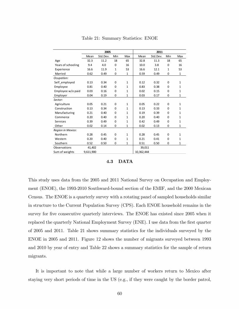
Table 21: Summary Statistics: ENOE

Mean Std.Dev. Min Max Mean Std.Dev. Min Max  Age 32.3 11.2 18 65 32.8 11.3 18 65  Years of schooling 9.4 4.0 0 16 10.0 3.8 0 16  Experience 16.6 11.9 1 53 16.6 12.1 1 53  Married 0.62 0.49 0 1 0.59 0.49 0 1Ocupation: Self_employed 0.13 0.34 0 1 0.12 0.32 0 1 Employee 0.81 0.40 0 1 0.83 0.38 0 1 Employee w/o paid 0.03 0.16 0 1 0.02 0.15 0 1 Employer 0.04 0.19 0 1 0.03 0.17 0 1Sector:  Agriculture 0.05 0.21 0 1 0.05 0.22 0 1  Construction 0.13 0.34 0 1 0.13 0.33 0 1  Manufacturing 0.21 0.40 0 1 0.19 0.39 0 1  Commerce 0.20 0.40 0 1 0.20 0.40 0 1  Services 0.39 0.49 0 1 0.42 0.49 0 1  Other 0.02 0.14 0 1 0.02 0.13 0 1Region in Mexico:  Northern 0.28 0.45 0 1 0.28 0.45 0 1  Western 0.20 0.40 0 1 0.21 0.41 0 1  Southern 0.52 0.50 0 1 0.51 0.50 0 1Observations 41,402 39,011Sum of weights 9,611,900 10,362,444

2005 2011

4.3 DATA

This study uses data from the 2005 and 2011 National Survey on Occupation and Employ-

ment (ENOE), the 1993-2010 Southward-bound section of the EMIF, and the 2000 Mexican

Census. The ENOE is a quarterly survey with a rotating panel of sampled households similar

in structure to the Current Population Survey (CPS). Each ENOE household remains in the

survey for �ve consecutive quarterly interviews. The ENOE has existed since 2005 when it

replaced the quarterly National Employment Survey (ENE). I use data from the �rst quarter

of 2005 and 2011. Table 21 shows summary statistics for the individuals surveyed by the

ENOE in 2005 and 2011. Figure 12 shows the number of migrants surveyed between 1993

and 2010 by year of entry and Table 22 shows a summary statistics for the sample of return

migrants.

It is important to note that while a large number of workers return to Mexico after

staying very short periods of time in the US (e.g., if they were caught by the border patrol,

60

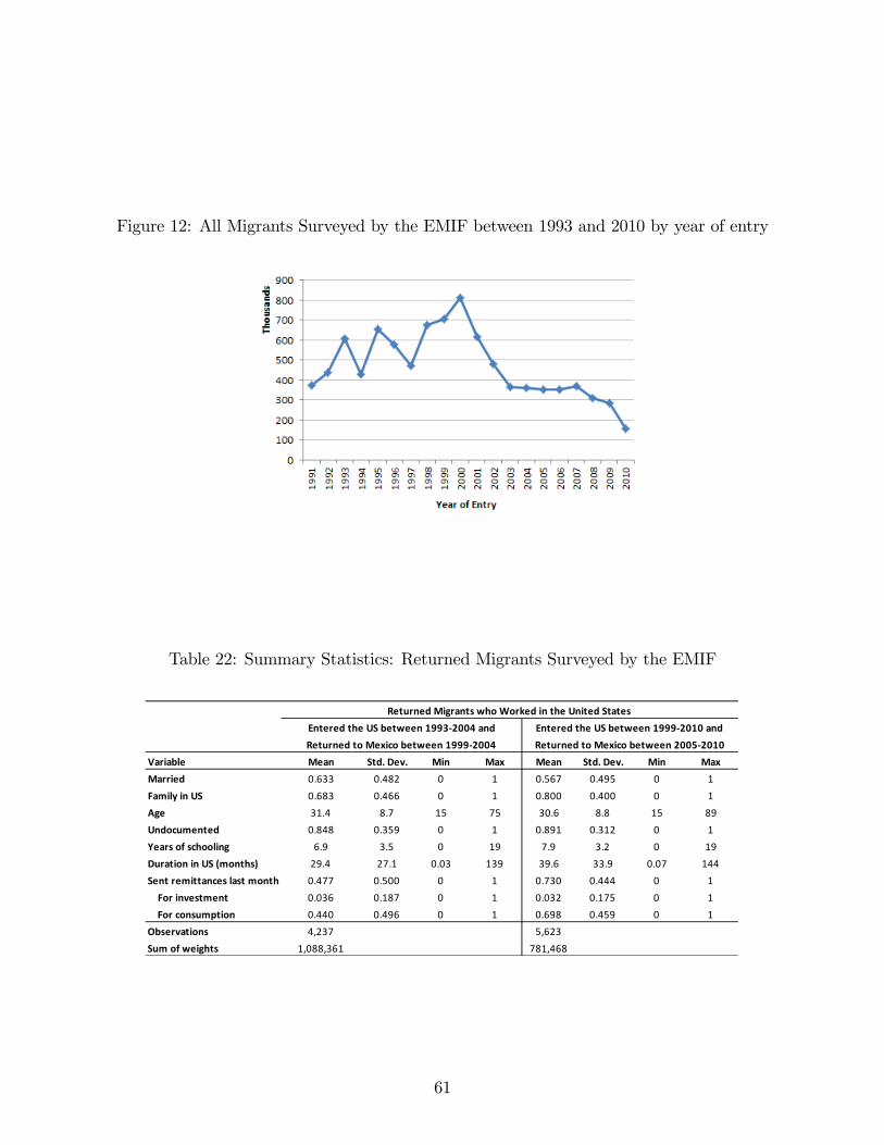
Figure 12: All Migrants Surveyed by the EMIF between 1993 and 2010 by year of entry

Table 22: Summary Statistics: Returned Migrants Surveyed by the EMIF

Variable Mean Std. Dev. Min Max Mean Std. Dev. Min MaxMarried 0.633 0.482 0 1 0.567 0.495 0 1Family in US 0.683 0.466 0 1 0.800 0.400 0 1Age 31.4 8.7 15 75 30.6 8.8 15 89Undocumented 0.848 0.359 0 1 0.891 0.312 0 1Years of schooling 6.9 3.5 0 19 7.9 3.2 0 19Duration in US (months) 29.4 27.1 0.03 139 39.6 33.9 0.07 144Sent remittances last month 0.477 0.500 0 1 0.730 0.444 0 1    For investment 0.036 0.187 0 1 0.032 0.175 0 1    For consumption 0.440 0.496 0 1 0.698 0.459 0 1Observations 4,237 5,623Sum of weights 1,088,361 781,468

Returned Migrants who Worked in the United StatesEntered the US between 1993­2004 andReturned to Mexico between 1999­2004

Entered the US between 1999­2010 andReturned to Mexico between 2005­2010

61

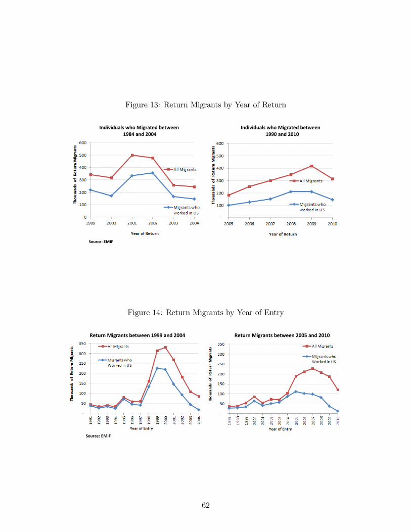
Figure 13: Return Migrants by Year of Return

Individuals who Migrated between1984 and 2004

Individuals who Migrated between1990 and 2010

Source: EMIF

Figure 14: Return Migrants by Year of Entry

Return Migrants between 1999 and 2004 Return Migrants between 2005 and 2010

Source: EMIF

62

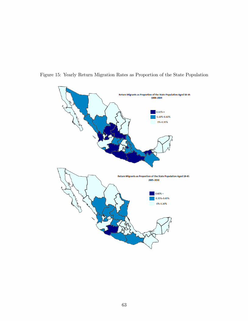
Figure 15: Yearly Return Migration Rates as Proportion of the State Population

63

or if they were not successful �nding a job in the US), migrants who enter the US and get a

job stay on average 33 months in the United States before they decide to return to Mexico.

Figure 13 shows the total number of return migrants between 1999 and 2010 by year of

return. Between 1999 and 2004 the number of return migrants who return after staying

a short period of time in the US decreases, however, starting in 2005 that number starts

increasing again and represents in 2010 more than 50 percent of the total number of return

migrants.

This issue is relevant since an increase in the total number of return migrants driven by

an increase of individuals who spend only short periods of time in the United States will not

increases the probability of self-employment in Mexico. Figure 14 shows the total number

of return migrants between 1999 and 2004 and between 2005 and 2010 by year of entry, and

the number of migrants who return to Mexico after working in the United States.

Figure 15 shows the average number of return migrants per year as proportion of the state

population aged 18-45 for the period 1999-2004 and 2005-2010. Over time there has been a

decrease in the number of return migrants as proportion of the total population. The average

for all states went from 0.40% between 1999 and 2004 to 0.26% between 2005 and 2010. It

is important to note that Figure 15 only includes return migrants who worked in the United

States. Including all return migrants might give very di¤erent results especially for states in

Southern Mexico (Tabasco, Oaxaca, Quintana Roo, Veracruz, Puebla, and Chiapas), states

that historically have had low migration rates, and therefore, do not have large migration

networks in the United States.

4.4 SELF-EMPLOYMENT AND RETURN MIGRATION IN MEXICO

I use the 2010 Mexican Census to analyze what is the relationship between self-employment,

return migration and earnings. Table 23 shows average wages, self-employment and unem-

ployment rates in Mexico, and Table 24 shows regression results. The �ndings show that

return migrants are more likely to be self-employed. Self-employed workers earn lower wages

than wage-workers, and that �nding is especially strong among non-return migrants. Addi-

64

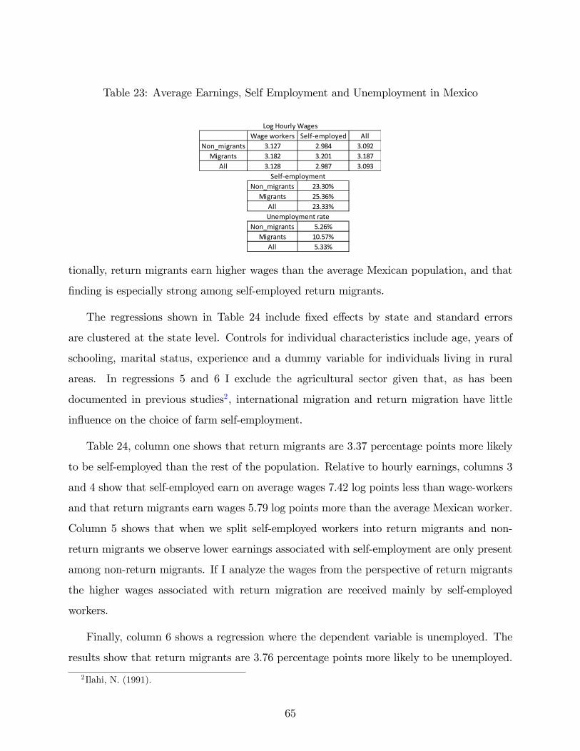
Table 23: Average Earnings, Self Employment and Unemployment in Mexico

Wage workers Self­employed AllNon_migrants 3.127 2.984 3.092

Migrants 3.182 3.201 3.187All 3.128 2.987 3.093

Non_migrants 23.30%Migrants 25.36%

All 23.33%

Non_migrants 5.26%Migrants 10.57%

All 5.33%

Log Hourly Wages

Unemployment rate

Self­employment

tionally, return migrants earn higher wages than the average Mexican population, and that

�nding is especially strong among self-employed return migrants.

The regressions shown in Table 24 include �xed e¤ects by state and standard errors

are clustered at the state level. Controls for individual characteristics include age, years of

schooling, marital status, experience and a dummy variable for individuals living in rural

areas. In regressions 5 and 6 I exclude the agricultural sector given that, as has been

documented in previous studies2, international migration and return migration have little

in�uence on the choice of farm self-employment.

Table 24, column one shows that return migrants are 3.37 percentage points more likely

to be self-employed than the rest of the population. Relative to hourly earnings, columns 3

and 4 show that self-employed earn on average wages 7.42 log points less than wage-workers

and that return migrants earn wages 5.79 log points more than the average Mexican worker.

Column 5 shows that when we split self-employed workers into return migrants and non-

return migrants we observe lower earnings associated with self-employment are only present

among non-return migrants. If I analyze the wages from the perspective of return migrants

the higher wages associated with return migration are received mainly by self-employed

workers.

Finally, column 6 shows a regression where the dependent variable is unemployed. The

results show that return migrants are 3.76 percentage points more likely to be unemployed.

2Ilahi, N. (1991).

65

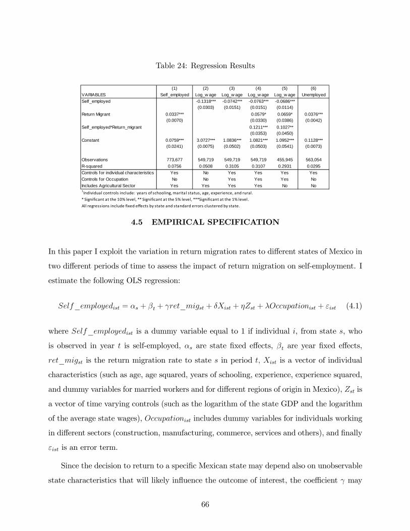
Table 24: Regression Results

(1) (2) (3) (4) (5) (6)VARIABLES Self_employed Log_w age Log_w age Log_w age Log_w age UnemployedSelf_employed ­0.1318*** ­0.0742*** ­0.0763*** ­0.0686***

(0.0303) (0.0151) (0.0151) (0.0114)Return Migrant 0.0337*** 0.0579* 0.0659* 0.0376***

(0.0070) (0.0330) (0.0386) (0.0042)Self_employed*Return_migrant 0.1211*** 0.1027**

(0.0353) (0.0450)Constant 0.0759*** 3.0727*** 1.0836*** 1.0821*** 1.0952*** 0.1128***

(0.0241) (0.0075) (0.0502) (0.0503) (0.0541) (0.0073)

Observations 773,677 549,719 549,719 549,719 455,945 563,054R­squared 0.0756 0.0508 0.3105 0.3107 0.2931 0.0295Controls for individual characteristics Yes No Yes Yes Yes YesControls for Occupation No No Yes Yes Yes NoIncludes Agricultural Sector Yes Yes Yes Yes No No

* Significant at the 10% level, ** Significant at the 5% level, ***Significant at the 1% level.All regressions include fixed effects by state and standard errors clustered by state.

1Individual controls include:  years of schooling, marital status, age, experience, and rural.

4.5 EMPIRICAL SPECIFICATION

In this paper I exploit the variation in return migration rates to di¤erent states of Mexico in

two di¤erent periods of time to assess the impact of return migration on self-employment. I

estimate the following OLS regression:

Self_employedist = �s + �t + ret_migst + �Xist + �Zst + �Occupationist + "ist (4.1)

where Self_employedist is a dummy variable equal to 1 if individual i, from state s, who

is observed in year t is self-employed, �s are state �xed e¤ects, �t are year �xed e¤ects,

ret_migst is the return migration rate to state s in period t; Xist is a vector of individual

characteristics (such as age, age squared, years of schooling, experience, experience squared,

and dummy variables for married workers and for di¤erent regions of origin in Mexico), Zst is

a vector of time varying controls (such as the logarithm of the state GDP and the logarithm

of the average state wages), Occupationist includes dummy variables for individuals working

in di¤erent sectors (construction, manufacturing, commerce, services and others), and �nally

"ist is an error term.

Since the decision to return to a speci�c Mexican state may depend also on unobservable

state characteristics that will likely in�uence the outcome of interest, the coe¢ cient may

66

be biased. For example, if there is selectivity of return migrants, if there are di¤erences

in the distribution of entrepreneurial abilities of workers who decide to stay in the US and

workers who return to Mexico, or if there exist di¤erences in the entrepreneurial incentives

faced by individuals returning to di¤erent Mexican states.

If return migrants are positively selected in terms of their entrepreneurial abilities, OLS

results may overestimate the real e¤ect, and underestimate it if return migrants are negatively

selected. Additionally, if migrants decide to return to states that provide their citizens

education and incentives to create businesses and become self-employed, the OLS results may

overestimate the real e¤ect. On the other hand, if individuals decide to migrate from and

return to states in which citizens face di¢ culties and barriers to enter self-employment, the

OLS results may underestimate the e¤ect of return migration on the self-employment rates

across Mexican states. One solution to this particular problem is the use of an instrument

that predicts return migration but exerts no impact on the outcome variable.

I use as instrument for return migration a predicted rate of return using migration rates

observed in the past for individuals from di¤erent Mexican states. I analyze two periods of

time, �rst I estimate the e¤ect of return migration between 1999 and 2004 on the decision to

become self-employed, and then for the period between 2005 and 2011. In order to predict

the return migration rates to di¤erent Mexican states during the �rst period of time (1999-

2004) I use the migration rates observed between 1993 and 1999, and for the second period

of analysis (2005-2010) I use the migration rates observed between 1999 and 2004.

The predicted return migration rates for the period between 1999 and 2004 are calculated

as follows:

1. Find the likelihood that an individual surveyed by the EMIF, who migrated between

1993 and 1998, and worked in an speci�c state in the US, was born in a particular state

of Mexico.

2. Estimate the total number of return migrants between 1999 and 2004 by state of residence

in the United States. The number of return migrants is calculated restricting the sample

to include individuals and who entered the United States between 1993 and 2004 and

had a job in the United States.

67

3. Using the probability that an individual residing in an speci�c state of the US was born

in a particular state of Mexico calculated in part 1, and the total number of return

migrants by state of residence in the US calculated in part 2, I predict the number of

return migrants from each state in the United States that will return to di¤erent states

in Mexico.

4. Estimate the number of return migrants per year to each Mexican state.

5. Calculate the number return migrants as proportion of the total population aged 18 to 65

of each state of Mexico according to the 2000 Mexican Count of Population and Housing.

In order to estimate the predicted return migration rates for the period between 2005

and 2010 I follow steps 1 through 5 using the sample of immigrants surveyed by the EMIF

who migrated between 1999 and 2004 for step 1, the number of return migrants between

2005 and 2010 who entered the US between 1999 and 2010 for step 2, and data from the

2000 Mexican Count of Population and Housing for step 5. Finally, equation 4.1 is estimated

using the predicted return migration rates as instrument.

The OLS and IV regressions are estimated restricting the sample to include males who

are part of the labor force, who were born in Mexico, and are aged 18 to 45. Additionally,

I restrict the sample to include only individuals working in non-agricultural activities in

urban areas, and include only individuals who became self-employed or who took a wage

work during the 5 years prior to the time of the survey.

4.6 RESULTS

The top panel of Table 25 shows the OLS regression results. An increase of one percent in

the number of return migrants as proportion of the total population (aged 18-45) increases

self-employment between 1.6 and 2.1 percentage points. It is important to note that these

magnitudes are considerably small and all the speci�cations are only statistically signi�cant

at the ten percent level.

The results using OLS regression can be potentially biased if the decision to return to a

68

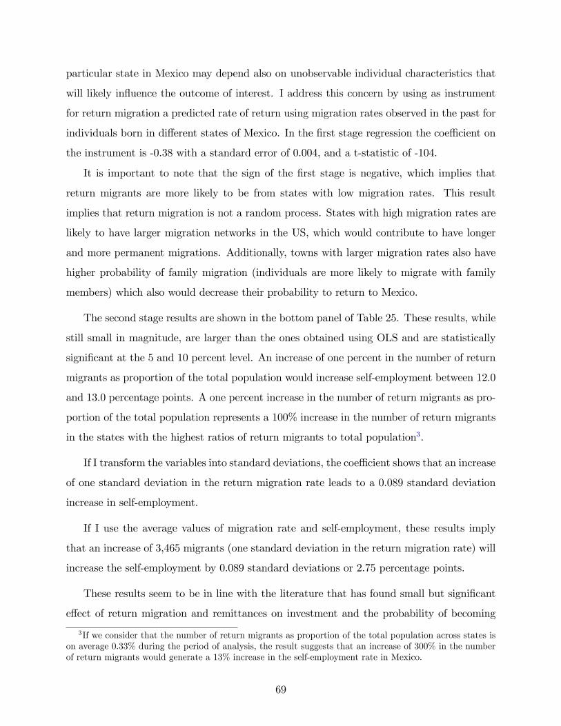
particular state in Mexico may depend also on unobservable individual characteristics that

will likely in�uence the outcome of interest. I address this concern by using as instrument

for return migration a predicted rate of return using migration rates observed in the past for

individuals born in di¤erent states of Mexico. In the �rst stage regression the coe¢ cient on

the instrument is -0.38 with a standard error of 0.004, and a t-statistic of -104.

It is important to note that the sign of the �rst stage is negative, which implies that

return migrants are more likely to be from states with low migration rates. This result

implies that return migration is not a random process. States with high migration rates are

likely to have larger migration networks in the US, which would contribute to have longer

and more permanent migrations. Additionally, towns with larger migration rates also have

higher probability of family migration (individuals are more likely to migrate with family

members) which also would decrease their probability to return to Mexico.

The second stage results are shown in the bottom panel of Table 25. These results, while

still small in magnitude, are larger than the ones obtained using OLS and are statistically

signi�cant at the 5 and 10 percent level. An increase of one percent in the number of return

migrants as proportion of the total population would increase self-employment between 12.0

and 13.0 percentage points. A one percent increase in the number of return migrants as pro-

portion of the total population represents a 100% increase in the number of return migrants

in the states with the highest ratios of return migrants to total population3.

If I transform the variables into standard deviations, the coe¢ cient shows that an increase

of one standard deviation in the return migration rate leads to a 0.089 standard deviation

increase in self-employment.

If I use the average values of migration rate and self-employment, these results imply

that an increase of 3,465 migrants (one standard deviation in the return migration rate) will

increase the self-employment by 0.089 standard deviations or 2.75 percentage points.

These results seem to be in line with the literature that has found small but signi�cant

e¤ect of return migration and remittances on investment and the probability of becoming

3If we consider that the number of return migrants as proportion of the total population across states ison average 0.33% during the period of analysis, the result suggests that an increase of 300% in the numberof return migrants would generate a 13% increase in the self-employment rate in Mexico.

69

Table 25: Regression Results

I. OLS ResultsDependent variable: Self­employment (1) (2) (3) (4)Return Migrants/Population 0.017* 0.016* 0.014 0.021*

(0.0090) (0.0090) (0.0110) (0.0120)ObservationsIncludes year fixed effects Yes Yes Yes YesIncludes state fixed effects Yes Yes Yes YesIncludes individual controls No Yes Yes YesIncludes time varying controls No No Yes YesIncludes controls for job characteristics No No No YesSample weights Yes Yes Yes Yes

II. Instrumental Variables  ResultDependent variable: Self­employment (1) (2) (3) (4)Return Migrants/Population 0.126* 0.124* 0.117** 0.130**

(0.0710) (0.0700) (0.0530) (0.0560)Observations 64,676 64,512 64,512 64,512Includes year fixed effects Yes Yes Yes YesIncludes state fixed effects Yes Yes Yes YesIncludes individual controls No Yes Yes YesIncludes time varying controls No No Yes YesIncludes controls for job characteristics No No No YesSample weights Yes Yes Yes Yes      First Stage Instrumental VariableDependent variable: Return Migrants/Population (1) (2) (3) (4)Instrument ­0.3538*** ­0.3544*** ­0.3835*** ­0.3834***

(0.0046) (0.0046) (0.0037) (0.0037)* Si gni ficant at the 10% l evel , ** Si gni ficant at the 5% l evel , *** Signi fi cant at the 1% l evel .

Time varying controls  include log GDP and log wa ges .Job characteris tics  include dummy variables  for di fferent industries : costruction, manufacturing, comerce, servicesand others .Standard errors are clustered at the state by year level.

Individual  controls  include age, age squared, married, years  of school ing, experience, experience squared, region oforigin in Mexico.

70

self-employed. That occurs when remittances tend to be disproportionately used for con-

sumption and non-productive investment. If remittances are primarily spent in conspicuous

consumption and non-productive investments, return migration may be conducive of in-

creases in leisure among household members. Another explanation, supported by Murillo

Castaño (1988) in his study of Colombian return migrants from Venezuela is that savings

(remittances) are used to establish, or expand self-employment activities but only after ba-

sic needs of the household members have been satis�ed. Therefore, if return migrants are

spending remittances satisfying the basic needs of their families, the e¤ect on investment

and self-employment would be very limited.

In order to verify if those arguments are valid for the case of Mexican return migrants, I

use data on the uses of remittances reported by workers surveyed by the EMIF. I restrict the

sample to include only return migrants who entered the US and returned to Mexico between

1993 and 2010 and sent remittances during their last month in the United States (50% of

the migrants who returned between 1993 and 2003 sent remittances during their last month

in the US and 70% of those who returned between 2005 and 2010).

It is important to note that the information on uses of remittances has to be interpreted

carefully. The survey inquires migrants about the use of remittances they sent the month

prior they returned to Mexico. I do not have information of the use of remittances for those

individuals who did not send remittances and who brought their remittances with them

when they return to Mexico. Individuals who know they will return within one month,

might prefer to bring the money with them instead of paying fees to send the remittances.

Therefore, if individuals planning to invest remittances upon return are also more likely to

bring the remittances with them, then these results might underestimate the likelihood of

using remittances for investment purposes. However, if that is the case, we can still see from

these data that over time a larger proportion of workers sent remittances the month before

they returned to Mexico, which implies that over time, the proportion of migrants using

remittances for consumption rather than for investment purposes has increased.

As Figure 16 shows, a large number of return migrants report that remittances are used

for consumption. While 77% of the migrants reported that remittances were spent on the

71

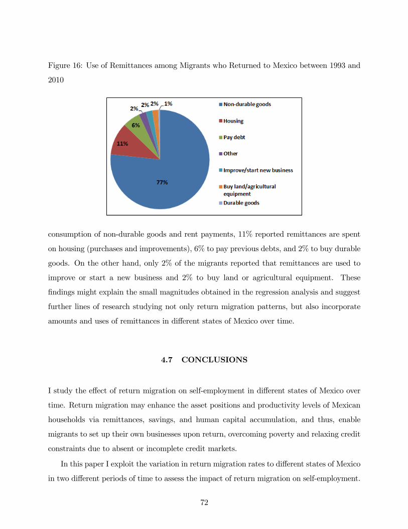
Figure 16: Use of Remittances among Migrants who Returned to Mexico between 1993 and

2010

consumption of non-durable goods and rent payments, 11% reported remittances are spent

on housing (purchases and improvements), 6% to pay previous debts, and 2% to buy durable

goods. On the other hand, only 2% of the migrants reported that remittances are used to

improve or start a new business and 2% to buy land or agricultural equipment. These

�ndings might explain the small magnitudes obtained in the regression analysis and suggest

further lines of research studying not only return migration patterns, but also incorporate

amounts and uses of remittances in di¤erent states of Mexico over time.

4.7 CONCLUSIONS

I study the e¤ect of return migration on self-employment in di¤erent states of Mexico over

time. Return migration may enhance the asset positions and productivity levels of Mexican

households via remittances, savings, and human capital accumulation, and thus, enable

migrants to set up their own businesses upon return, overcoming poverty and relaxing credit

constraints due to absent or incomplete credit markets.

In this paper I exploit the variation in return migration rates to di¤erent states of Mexico

in two di¤erent periods of time to assess the impact of return migration on self-employment.

72

I estimate OLS regressions and in order to avoid potential endogeneity issues I also use

instrumental variables. I use as instrument for return migration a predicted rate of return

using migration rates observed in the past in di¤erent Mexican states.

Using instrumental variables the results show that return migration exerted a positive but

small impact on the probability of creating non-farm business in Mexico between 1999 and

2011. An increase of one percent in the number of return migrants measured as proportion

of the state population increases the probability of being self-employed by 13 percentage

points.

The results seem to be in line with the literature that has found very small e¤ect of

return migration and remittances on investment and the decision to become self-employed

which occurs when remittances tend to be disproportionately used for consumption and

non-productive investment. In order to verify if those arguments are valid for the case of

Mexican return migrants, I use data on the uses of remittances reported by workers who

returned to Mexico between 1993 and 2010. The evidence shows that remittances are used

predominantly for consumption purposes. While 77% of the return migrants reported that

remittances were spent on the consumption of non-durable goods and rent payments, 11%

reported were spent on housing, 6% to pay previous debts, and 2% to buy durable goods.

On the other hand, only 2% of the migrants reported that remittances were used to improve

or start a new business and 2% to buy land or agricultural equipment. These �ndings might

explain the small magnitudes obtained in the regression analysis and suggest further lines

of research studying not only return migration patterns, but also the amount of remittances

and the uses of remittances in di¤erent states of Mexico over time.

73

5.0 DRUG VIOLENCE AND MIGRATION FLOWS

5.1 MOTIVATION

In recent years, Mexico has experienced a dramatic surge in homicides driven in large part

by the violent struggle between and within powerful criminal organizations to control the

lucrative drug trade business. E¤orts by President Felipe Calderon�s administration to com-

bat organized crime have resulted in a signi�cant increase in killings. Between 2006 and

2011, 47,5151 killings were o¢ cially linked to organized crime, a dramatic increase from the

8,901 killings recorded under President Vicente Fox�s administration (2000 - 2006).2 While

there is consensus that drug violence has had social, economic and political impact, little re-

search has been devoted to study the e¤ect of violence on the migratory patterns of Mexican

workers.

During the period of 2006-2012 the number of Mexican immigrants in the US decreased

signi�cantly. According to Passel et al. (2012), in 2010 for the �rst time in four decades

the net �ow of immigrants from Mexico to the United States was zero. Some of the factors

that could have contributed to the change in the migratory behavior of Mexican immigrants

are the recession su¤ered by the United States since 2008, the creation of unfavorable State

immigration laws for undocumented immigrants, and the increase in violence generated by

the war against drug tra¢ cking in Mexico.

Violence can a¤ect the in�ows and out�ows of migrants; however, it is not clear in which

direction the e¤ects go. Violence creates a social and economic burden on societies, and

1Estimates from December 2006 to September 2011. Source: ENVIPE.2Rios V., Shirk D. (2011).

74

impacts not only individuals or businesses, but also the larger economy. Estimates suggest

that the annual cost of violence in Mexico is between 1.0 and 1.5% of GDP,3 it decreases

foreign direct investment, domestic investment, and personal consumption, but can also

a¤ect individuals�earnings, job performance or the ability to keep a job.

Additionally, violence imposes signi�cant emotional costs on individuals. Violence gen-

erates displacement; individuals tend to migrate in order to �nd safer environments for them

and their families. It is documented that US cities in the southern border have seen a relative

increase of middle-class Mexican migration associated to the increase in violence in Mexico

(Arceo-Gomez (2012) and Becker (2009)).

The increase in violence could have also changed the emotional cost of being away,

increasing the cost for migrants who leave their families back in Mexico who perceive their

family members might be at risk; and decreasing the cost of migrants who migrate with their

families to the US and now feel that Mexico is not a good place to be.

Migration costs could have also increased with violence. During the last years crimi-

nal gangs have come to control smuggling routes into the United States and migrants are

frequently subjects of abuses including assault, extortion, theft, and death at the hands of

those violent criminal groups.4

In this chapter I study the e¤ect of drug-violence on the out�ow of immigrants from

Mexico to the United States. I exploit the variation in violence across municipalities over the

period of 2007-2011 using data of homicides due to rivalry between delinquent organizations

and data on Mexican migration from the Surveys of Migration to the Northern Border

(EMIF).

The results show that the increase in violence a¤ects di¤erently the out�ows of migrants

3According to JP Morgan the annual cost of violence in Mexico is estimated to be between 1 and 1.5% ofGDP. BBVA Bancomer also estimated the cost between 1 and 1.5% of GDP. INEGI estimated that the costin 2010 was 1.53% of the GDP using the ENVIPE for 2011. Excelsior (09/06/2011): "JP Morgan revela quela violencia en México cuesta 1.5% del PIB". http://www.excelsior.com.mx/2011/06/09/dinero/743660.

4The Mexican government has advised migrants driving home from the US for the winter holidays toform convoys for their own protection inside Mexico and to travel only during daylight hours. The interiorministry said the Mexican army could provide escorts to protect convoys from attacks of criminal groups.Source: "Mexico migrants told to form convoys," BBC, Nov 22, 2010. http://www.bbc.co.uk/news/world-latin-america-11815381

75

from di¤erent regions of Mexico. While an increase in violence is associated with an increase

in the out�ows of migrants from Western Mexico, it is also associated with a decrease in the

out�ows of individuals from Southern Mexico. An increase of 1 death per 10,000 inhabitants

increases migration rates from municipalities of Western Mexico by 0.06 percentage points,

but decreases migration rates from municipalities of Southern Mexico by 0.10 percentage

points.

Similarly, when I use the sample of migrants caught by the Border Patrol and study their

probability of re-entry, an increase of 1 death per 10,000 inhabitants in their municipality

of origin increases the probability to try to re-enter the US by 0.43 percentage points for

individuals from Western Mexico, but decreases the probability to try to re-enter by 0.33

percentage points for migrants from Southern Mexico.

One factor that could explain the di¤erences in the behavior of workers from Western

and Southern Mexico is having di¤erent costs associated with the increase in violence, for

example, if individuals from di¤erent regions of Mexico su¤er di¤erent changes in earnings

or migration cost. In order to test for such di¤erences I use Mexico�s 2011 and 2012 National

Survey on Victimization and Perceptions of Public Safety (ENVIPE). This survey provides

estimates of the number of crime victims, economic losses due to crime, as well as perceptions

of public safety at the national and sub-national levels. The results show that individuals

fromWestern Mexico feel more unsafe in their own municipality and have higher losses due to

crime. Therefore, the high costs associated with increases in violence could have contributed

to the increase in the out�ow of workers from that region of Mexico.

5.2 LITERATURE REVIEW

Most of the research studying the e¤ect of the increase in violence on the behavior of Mex-

ican migrants has analyzed how US cities on the US-Mexico border have seen a relative

increase of middle-class Mexican migration (Arceo-Gomez (2012)). Unlike the traditional

job-seeking migrants, this new migrant class comprises business owners, executives and other

professionals who have established new businesses in US cities creating jobs and investing in

76

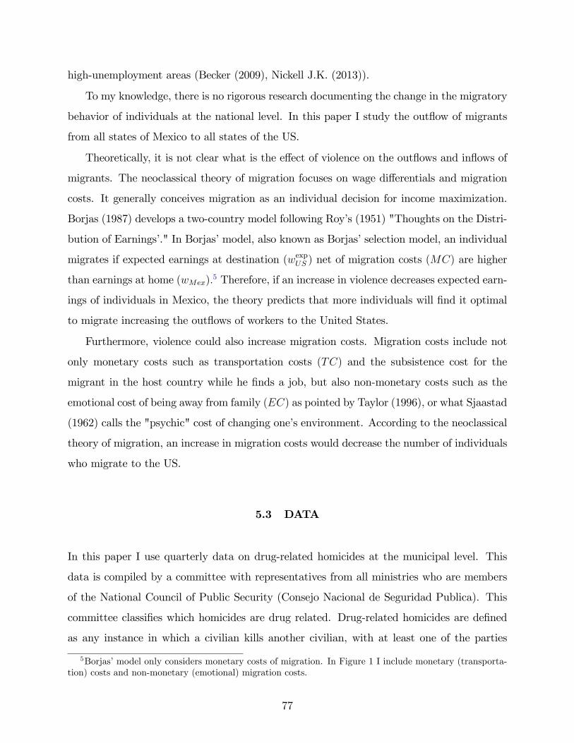
high-unemployment areas (Becker (2009), Nickell J.K. (2013)).

To my knowledge, there is no rigorous research documenting the change in the migratory

behavior of individuals at the national level. In this paper I study the out�ow of migrants

from all states of Mexico to all states of the US.

Theoretically, it is not clear what is the e¤ect of violence on the out�ows and in�ows of

migrants. The neoclassical theory of migration focuses on wage di¤erentials and migration

costs. It generally conceives migration as an individual decision for income maximization.

Borjas (1987) develops a two-country model following Roy�s (1951) "Thoughts on the Distri-

bution of Earnings�." In Borjas�model, also known as Borjas�selection model, an individual

migrates if expected earnings at destination (wexpUS ) net of migration costs (MC) are higher

than earnings at home (wMex):5 Therefore, if an increase in violence decreases expected earn-

ings of individuals in Mexico, the theory predicts that more individuals will �nd it optimal

to migrate increasing the out�ows of workers to the United States.

Furthermore, violence could also increase migration costs. Migration costs include not

only monetary costs such as transportation costs (TC) and the subsistence cost for the

migrant in the host country while he �nds a job, but also non-monetary costs such as the

emotional cost of being away from family (EC) as pointed by Taylor (1996), or what Sjaastad

(1962) calls the "psychic" cost of changing one�s environment. According to the neoclassical

theory of migration, an increase in migration costs would decrease the number of individuals

who migrate to the US.

5.3 DATA

In this paper I use quarterly data on drug-related homicides at the municipal level. This

data is compiled by a committee with representatives from all ministries who are members

of the National Council of Public Security (Consejo Nacional de Seguridad Publica). This

committee classi�es which homicides are drug related. Drug-related homicides are de�ned

as any instance in which a civilian kills another civilian, with at least one of the parties

5Borjas�model only considers monetary costs of migration. In Figure 1 I include monetary (transporta-tion) costs and non-monetary (emotional) migration costs.

77

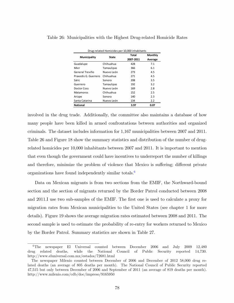
Table 26: Municipalities with the Highest Drug-related Homicide Rates

Total Monthly2007­2011 Average

Guadalupe Chihuahua 428 7.1Mier Tamaulipas 366 6.1General Treviño Nuevo León 273 4.5Praxedis G. Guerrero Chihuahua 271 4.5Sáric Sonora 208 3.5Guerrero Tamaulipas 192 3.2Doctor Coss Nuevo León 169 2.8Matamoros Chihuahua 152 2.5Arizpe Sonora 140 2.3Santa Catarina Nuevo León 134 2.2National 3.97 0.07

Drug­related Homicides per 10,000 inhabitants

Municipality State

involved in the drug trade. Additionally, the committee also maintains a database of how

many people have been killed in armed confrontations between authorities and organized

criminals. The dataset includes information for 1,167 municipalities between 2007 and 2011.

Table 26 and Figure 18 show the summary statistics and distribution of the number of drug-

related homicides per 10,000 inhabitants between 2007 and 2011. It is important to mention

that even though the government could have incentives to underreport the number of killings

and therefore, minimize the problem of violence that Mexico is su¤ering; di¤erent private

organizations have found independently similar totals.6

Data on Mexican migrants is from two sections from the EMIF, the Northward-bound

section and the section of migrants returned by the Border Patrol conducted between 2008

and 2011.I use two sub-samples of the EMIF. The �rst one is used to calculate a proxy for

migration rates from Mexican municipalities to the United States (see chapter 1 for more

details). Figure 19 shows the average migration rates estimated between 2008 and 2011. The

second sample is used to estimate the probability of re-entry for workers returned to Mexico

by the Border Patrol. Summary statistics are shown in Table 27.

6The newspaper El Universal counted between December 2006 and July 2009 12,480drug related deaths, while the National Council of Public Security reported 14,730.http://www.eluniversal.com.mx/estados/72681.htmlThe newspaper Milenio counted between December of 2006 and December of 2012 58,000 drug re-

lated deaths (an average of 805 deaths per month). The National Council of Public Security reported47,515 but only between December of 2006 and September of 2011 (an average of 819 deaths per month).http://www.milenio.com/cdb/doc/impreso/9165950

78

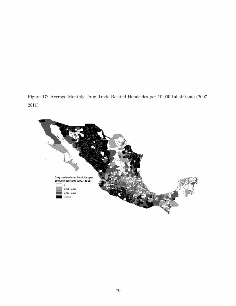
Figure 17: Average Monthly Drug Trade Related Homicides per 10,000 Inhabitants (2007-

2011)

79

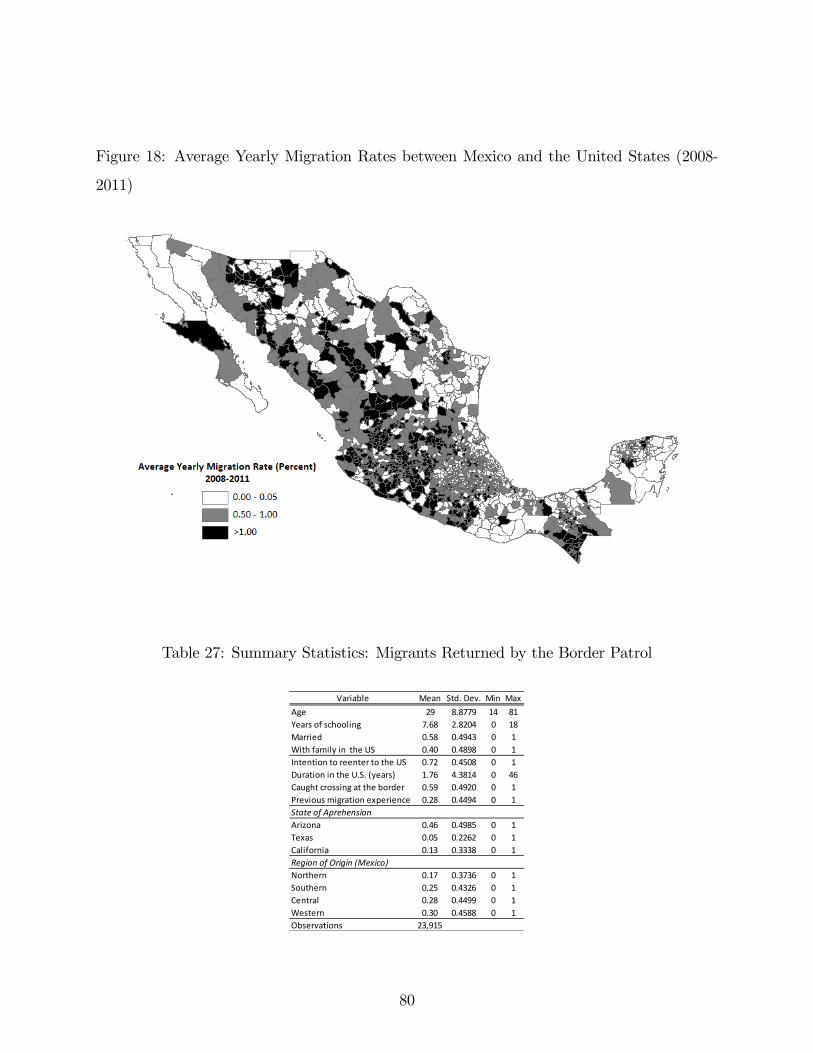
Figure 18: Average Yearly Migration Rates between Mexico and the United States (2008-

2011)

Table 27: Summary Statistics: Migrants Returned by the Border Patrol

Variable Mean Std. Dev. Min MaxAge 29 8.8779 14 81Years of schooling 7.68 2.8204 0 18Married 0.58 0.4943 0 1With family in  the US 0.40 0.4898 0 1Intention to reenter to the US 0.72 0.4508 0 1Duration in the U.S. (years) 1.76 4.3814 0 46Caught crossing at the border 0.59 0.4920 0 1Previous migration experience 0.28 0.4494 0 1State of AprehensionArizona 0.46 0.4985 0 1Texas 0.05 0.2262 0 1California 0.13 0.3338 0 1Region of Origin (Mexico)Northern 0.17 0.3736 0 1Southern 0.25 0.4326 0 1Central 0.28 0.4499 0 1Western 0.30 0.4588 0 1Observations 23,915

80

Finally, in order to verify if the cost of violence is di¤erent for individuals from di¤erent

regions of the country I use Mexico�s 2011 and 2012 National Survey on Victimization and

Perceptions of Public Safety (ENVIPE). This survey provides estimates of the number of

crime victims, economic losses due to crime, as well as perceptions of public safety at the

national and sub-national levels.

5.4 EMPIRICAL SPECIFICATION

5.4.1 E¤ect of Violence on the Out�ows of Migrants: Sample of Migrants who

Intend to Enter the US

In order to study the e¤ect of the increase in drug-related violence on the out�ows of mi-

grants from Mexico to the United States I use two di¤erent sub-samples. The �rst survey

is conducted among migrants in border cities who left their hometowns and moved to the

US-Mexico border with intention to cross into the US to work or look for a job. Using this

dataset I test how the increase in violence is associated with changes in migration rates in

their municipality of origin. I use data of migrants from the EMIF between 2008 and 2011,

and data of population from the 2010 Mexican Census to construct migration rates at the

municipality level over time and run the following regression:

Migration_ratemt = �m + �t + 1deathsmt�1 + "mt

where Migration_ratemt is the number of migrants from municipality m in year t as a

proportion of the municipal population, deathsmt�1 is the number of homicides committed

in municipality m between 2007 and year t� 1 per 10,000 inhabitants, �m are municipality

�xed e¤ects, �t are year �xed e¤ects, and "mt is an error term.7

It is important to note that individuals from di¤erent regions of Mexico have di¤erent

characteristics, and therefore, might have been a¤ected di¤erently by changes in violence.

For example, municipalities from western Mexico have been traditionally source of migrants.

7The EMIF is not responded by migrants who reside in the border cities where the surveys are conducted.Therefore, the migration rate for most of these municipalities is underestimated. For that reason, I eliminatedfrom the regression all the municipalities located within 100 kilometers of the U.S.-Mexico border.

81

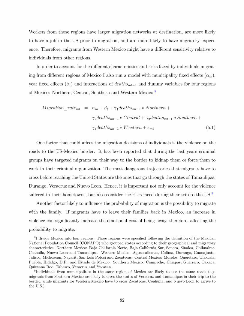
Workers from those regions have larger migration networks at destination, are more likely

to have a job in the US prior to migration, and are more likely to have migratory experi-

ence. Therefore, migrants from Western Mexico might have a di¤erent sensitivity relative to

individuals from other regions.

In order to account for the di¤erent characteristics and risks faced by individuals migrat-

ing from di¤erent regions of Mexico I also run a model with municipality �xed e¤ects (�m),

year �xed e¤ects (�t) and interactions of deathsmt�1 and dummy variables for four regions

of Mexico: Northern, Central, Southern and Western Mexico.8

Migration_ratemt = �m + �t + 1deathsmt�1 �Northern+

2deathsmt�1 � Central + 3deathsmt�1 � Southern+

4deathsmt�1 �Western+ "mt (5.1)

One factor that could a¤ect the migration decisions of individuals is the violence on the

roads to the US-Mexico border. It has been reported that during the last years criminal

groups have targeted migrants on their way to the border to kidnap them or force them to

work in their criminal organization. The most dangerous trajectories that migrants have to

cross before reaching the United States are the ones that go through the states of Tamaulipas,

Durango, Veracruz and Nuevo Leon. Hence, it is important not only account for the violence

su¤ered in their hometowns, but also consider the risks faced during their trip to the US.9

Another factor likely to in�uence the probability of migration is the possibility to migrate

with the family. If migrants have to leave their families back in Mexico, an increase in

violence can signi�cantly increase the emotional cost of being away, therefore, a¤ecting the

probability to migrate.

8I divide Mexico into four regions. These regions were speci�ed following the de�nition of the MexicanNational Population Council (CONAPO) who grouped states according to their geographical and migratorycharacteristics. Northern Mexico: Baja California Norte, Baja California Sur, Sonora, Sinaloa, Chihuahua,Coahuila, Nuevo Leon and Tamaulipas. Western Mexico: Aguascalientes, Colima, Durango, Guanajuato,Jalisco, Michoacan, Nayarit, San Luis Potosi and Zacatecas. Central Mexico: Morelos, Queretaro, Tlaxcala,Puebla, Hidalgo, D.F., and Estado de Mexico. Southern Mexico: Campeche, Chiapas, Guerrero, Oaxaca,Quintana Roo, Tabasco, Veracruz and Yucatan.

9Individuals from municipalities in the same region of Mexico are likely to use the same roads (e.g.migrants from Southern Mexico are likely to cross the states of Veracruz and Tamaulipas in their trip to theborder, while migrants for Western Mexico have to cross Zacatecas, Coahuila, and Nuevo Leon to arrive tothe U.S.)

82

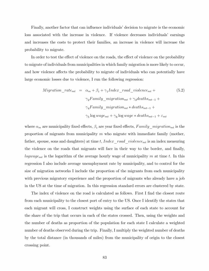
Finally, another factor that can in�uence individuals�decision to migrate is the economic

loss associated with the increase in violence. If violence decreases individuals� earnings

and increases the costs to protect their families, an increase in violence will increase the

probability to migrate.

In order to test the e¤ect of violence on the roads, the e¤ect of violence on the probability

to migrate of individuals frommunicipalities in which family migration is more likely to occur,

and how violence a¤ects the probability to migrate of individuals who can potentially have

large economic losses due to violence, I run the following regression:

Migration_ratemt = �m + �t + 1Index_road_violencemt + (5.2)

2Family_migrationmt + 3deathsmt�1 +

4Family_migrationmt � deathsmt�1 +

5 logwagemt + 6 logwage � deathsmt�1 + "mt

where �m are municipality �xed e¤ects, �t are year �xed e¤ects, Family_migrationmt is the

proportion of migrants from municipality m who migrate with immediate family (mother,

father, spouse, sons and daughters) at time t, Index_road_violencemt is an index measuring

the violence on the roads that migrants will face in their way to the border, and �nally,

logwagemt is the logarithm of the average hourly wage of municipality m at time t. In this

regression I also include average unemployment rate by municipality, and to control for the

size of migration networks I include the proportion of the migrants from each municipality

with previous migratory experience and the proportion of migrants who already have a job

in the US at the time of migration. In this regression standard errors are clustered by state.

The index of violence on the road is calculated as follows. First I �nd the closest route

from each municipality to the closest port of entry to the US. Once I identify the states that

each migrant will cross, I construct weights using the surface of each state to account for

the share of the trip that occurs in each of the states crossed. Then, using the weights and

the number of deaths as proportion of the population for each state I calculate a weighted

number of deaths observed during the trip. Finally, I multiply the weighted number of deaths

by the total distance (in thousands of miles) from the municipality of origin to the closest

crossing point.

83

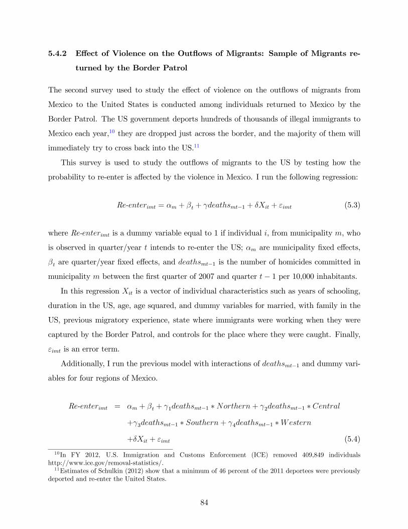
5.4.2 E¤ect of Violence on the Out�ows of Migrants: Sample of Migrants re-

turned by the Border Patrol

The second survey used to study the e¤ect of violence on the out�ows of migrants from

Mexico to the United States is conducted among individuals returned to Mexico by the

Border Patrol. The US government deports hundreds of thousands of illegal immigrants to

Mexico each year,10 they are dropped just across the border, and the majority of them will

immediately try to cross back into the US.11

This survey is used to study the out�ows of migrants to the US by testing how the

probability to re-enter is a¤ected by the violence in Mexico. I run the following regression:

Re-enterimt = �m + �t + deathsmt�1 + �Xit + "imt (5.3)

where Re-enterimt is a dummy variable equal to 1 if individual i, from municipality m, who

is observed in quarter/year t intends to re-enter the US; �m are municipality �xed e¤ects,

�t are quarter/year �xed e¤ects, and deathsmt�1 is the number of homicides committed in

municipality m between the �rst quarter of 2007 and quarter t� 1 per 10,000 inhabitants.

In this regression Xit is a vector of individual characteristics such as years of schooling,

duration in the US, age, age squared, and dummy variables for married, with family in the

US, previous migratory experience, state where immigrants were working when they were

captured by the Border Patrol, and controls for the place where they were caught. Finally,

"imt is an error term.

Additionally, I run the previous model with interactions of deathsmt�1 and dummy vari-

ables for four regions of Mexico.

Re-enterimt = �m + �t + 1deathsmt�1 �Northern+ 2deathsmt�1 � Central

+ 3deathsmt�1 � Southern+ 4deathsmt�1 �Western

+�Xit + "imt (5.4)

10In FY 2012, U.S. Immigration and Customs Enforcement (ICE) removed 409,849 individualshttp://www.ice.gov/removal-statistics/.11Estimates of Schulkin (2012) show that a minimum of 46 percent of the 2011 deportees were previously

deported and re-enter the United States.

84

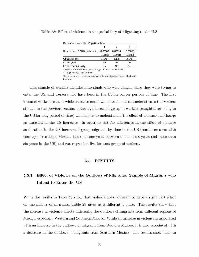
Table 28: E¤ect of violence in the probability of Migrating to the U.S.

Dependent variable: Migration Rate1 2 3

Deaths per 10,000 inhabitants ­0.00003 0.00014 ­0.00008(0.0001) (0.0001) (0.0002)

Observations 3,178 3,178 3,178FE per year No Yes YesFE per municipality No No Yes* Significant at the 10% level, ** Significant at the 5% level,***Significant at the 1% level.The regressions include sample weights and standard errors clusteredby state.

This sample of workers includes individuals who were caught while they were trying to

enter the US, and workers who have been in the US for longer periods of time. The �rst

group of workers (caught while trying to cross) will have similar characteristics to the workers

studied in the previous section; however, the second group of workers (caught after being in

the US for long period of time) will help us to understand if the e¤ect of violence can change

as duration in the US increases. In order to test for di¤erences in the e¤ect of violence

as duration in the US increases I group migrants by time in the US (border crossers with

country of residence Mexico, less than one year, between one and six years and more than

six years in the US) and run regression �ve for each group of workers.

5.5 RESULTS

5.5.1 E¤ect of Violence on the Out�ows of Migrants: Sample of Migrants who

Intend to Enter the US

While the results in Table 28 show that violence does not seem to have a signi�cant e¤ect

on the in�ows of migrants, Table 29 gives us a di¤erent picture. The results show that

the increase in violence a¤ects di¤erently the out�ows of migrants from di¤erent regions of

Mexico, especially Western and Southern Mexico. While an increase in violence is associated

with an increase in the out�ows of migrants from Western Mexico, it is also associated with

a decrease in the out�ows of migrants from Southern Mexico. The results show that an

85

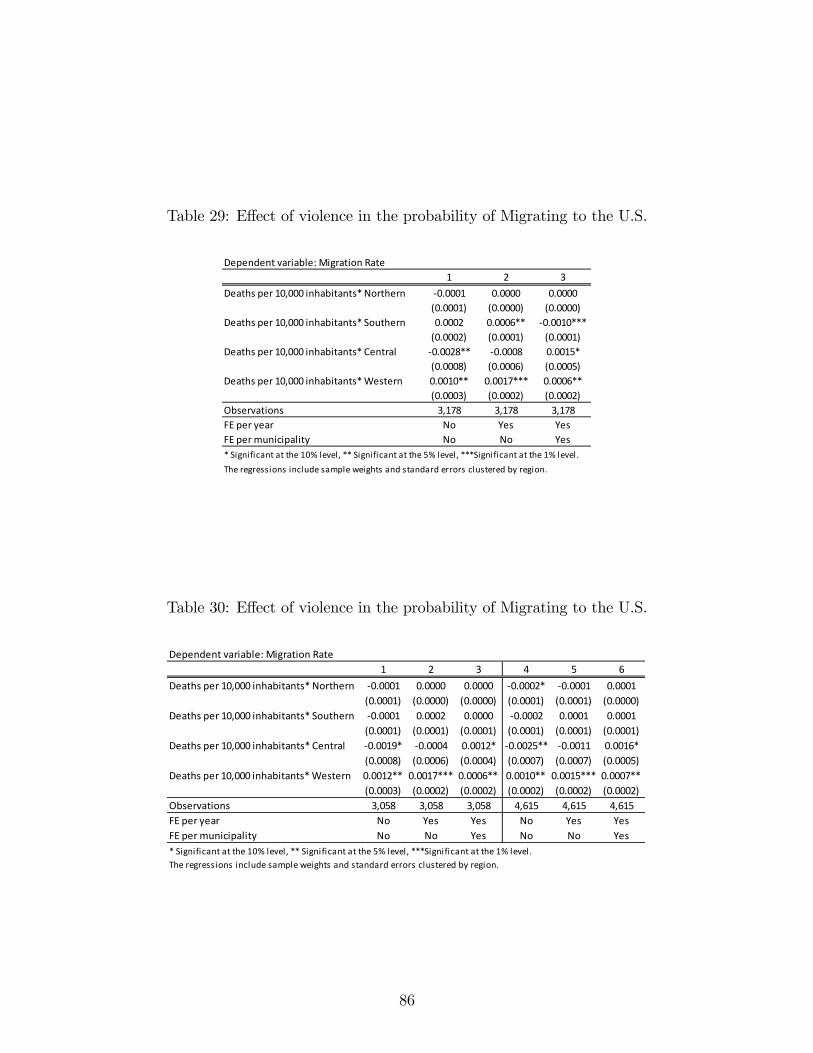
Table 29: E¤ect of violence in the probability of Migrating to the U.S.

Dependent variable: Migration Rate1 2 3

Deaths per 10,000 inhabitants* Northern ­0.0001 0.0000 0.0000(0.0001) (0.0000) (0.0000)

Deaths per 10,000 inhabitants* Southern 0.0002 0.0006** ­0.0010***(0.0002) (0.0001) (0.0001)

Deaths per 10,000 inhabitants* Central ­0.0028** ­0.0008 0.0015*(0.0008) (0.0006) (0.0005)

Deaths per 10,000 inhabitants* Western 0.0010** 0.0017*** 0.0006**(0.0003) (0.0002) (0.0002)

Observations 3,178 3,178 3,178FE per year No Yes YesFE per municipality No No Yes* Significant at the 10% level, ** Significant at the 5% level, ***Significant at the 1% level.The regressions include sample weights and standard errors clustered by region.

Table 30: E¤ect of violence in the probability of Migrating to the U.S.

Dependent variable: Migration Rate1 2 3 4 5 6

Deaths per 10,000 inhabitants* Northern ­0.0001 0.0000 0.0000 ­0.0002* ­0.0001 0.0001(0.0001) (0.0000) (0.0000) (0.0001) (0.0001) (0.0000)

Deaths per 10,000 inhabitants* Southern ­0.0001 0.0002 0.0000 ­0.0002 0.0001 0.0001(0.0001) (0.0001) (0.0001) (0.0001) (0.0001) (0.0001)

Deaths per 10,000 inhabitants* Central ­0.0019* ­0.0004 0.0012* ­0.0025** ­0.0011 0.0016*(0.0008) (0.0006) (0.0004) (0.0007) (0.0007) (0.0005)

Deaths per 10,000 inhabitants* Western 0.0012** 0.0017*** 0.0006** 0.0010** 0.0015*** 0.0007**(0.0003) (0.0002) (0.0002) (0.0002) (0.0002) (0.0002)

Observations 3,058 3,058 3,058 4,615 4,615 4,615FE per year No Yes Yes No Yes YesFE per municipality No No Yes No No Yes

The regressions include sample weights and standard errors clustered by region.* Significant at the 10% level, ** Significant at the 5% level, ***Significant at the 1% level.

86

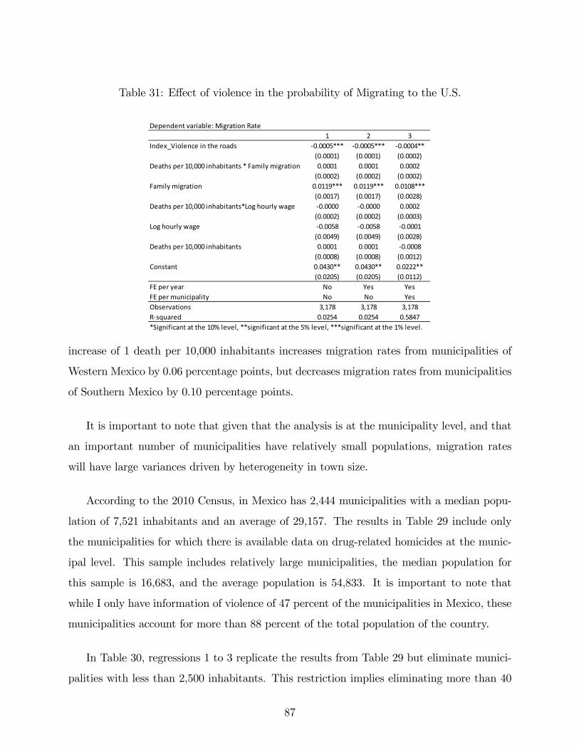
Table 31: E¤ect of violence in the probability of Migrating to the U.S.

Dependent variable: Migration Rate1 2 3

Index_Violence in the roads ­0.0005*** ­0.0005*** ­0.0004**(0.0001) (0.0001) (0.0002)

Deaths per 10,000 inhabitants * Family migration 0.0001 0.0001 0.0002(0.0002) (0.0002) (0.0002)

Family migration 0.0119*** 0.0119*** 0.0108***(0.0017) (0.0017) (0.0028)

Deaths per 10,000 inhabitants*Log hourly wage ­0.0000 ­0.0000 0.0002(0.0002) (0.0002) (0.0003)

Log hourly wage ­0.0058 ­0.0058 ­0.0001(0.0049) (0.0049) (0.0028)

Deaths per 10,000 inhabitants 0.0001 0.0001 ­0.0008(0.0008) (0.0008) (0.0012)

Constant 0.0430** 0.0430** 0.0222**(0.0205) (0.0205) (0.0112)

FE per year No Yes YesFE per municipality No No YesObservations 3,178 3,178 3,178R­squared 0.0254 0.0254 0.5847*Significant at the 10% level, **significant at the 5% level, ***significant at the 1% level.

increase of 1 death per 10,000 inhabitants increases migration rates from municipalities of

Western Mexico by 0.06 percentage points, but decreases migration rates from municipalities

of Southern Mexico by 0.10 percentage points.

It is important to note that given that the analysis is at the municipality level, and that

an important number of municipalities have relatively small populations, migration rates

will have large variances driven by heterogeneity in town size.

According to the 2010 Census, in Mexico has 2,444 municipalities with a median popu-

lation of 7,521 inhabitants and an average of 29,157. The results in Table 29 include only

the municipalities for which there is available data on drug-related homicides at the munic-

ipal level. This sample includes relatively large municipalities, the median population for

this sample is 16,683, and the average population is 54,833. It is important to note that

while I only have information of violence of 47 percent of the municipalities in Mexico, these

municipalities account for more than 88 percent of the total population of the country.

In Table 30, regressions 1 to 3 replicate the results from Table 29 but eliminate munici-

palities with less than 2,500 inhabitants. This restriction implies eliminating more than 40

87

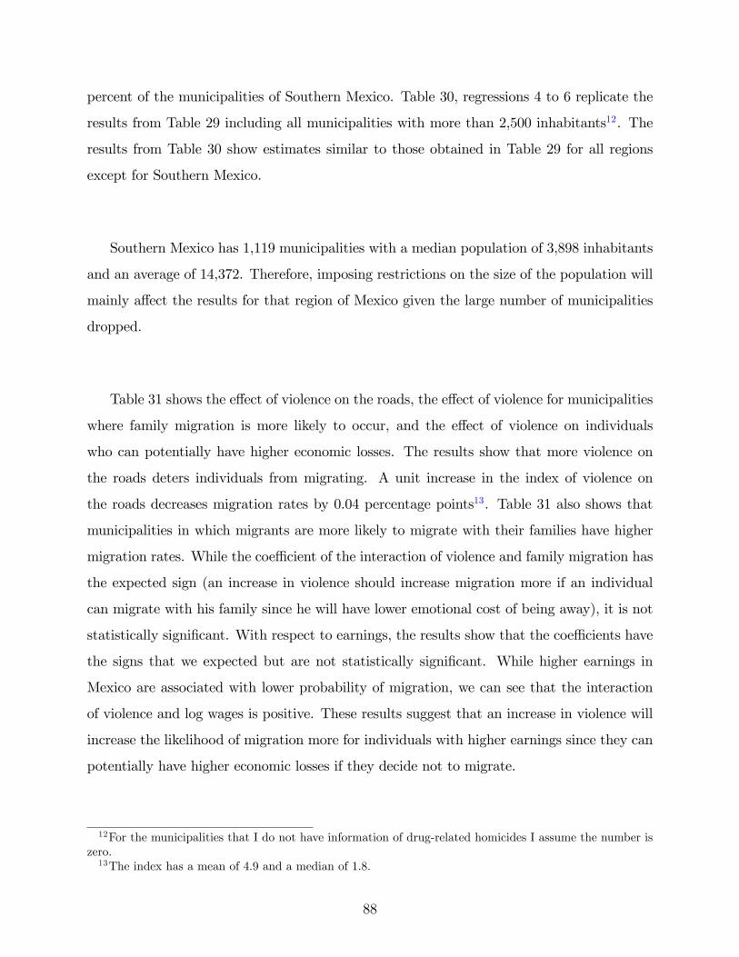
percent of the municipalities of Southern Mexico. Table 30, regressions 4 to 6 replicate the

results from Table 29 including all municipalities with more than 2,500 inhabitants12. The

results from Table 30 show estimates similar to those obtained in Table 29 for all regions

except for Southern Mexico.

Southern Mexico has 1,119 municipalities with a median population of 3,898 inhabitants

and an average of 14,372. Therefore, imposing restrictions on the size of the population will

mainly a¤ect the results for that region of Mexico given the large number of municipalities

dropped.

Table 31 shows the e¤ect of violence on the roads, the e¤ect of violence for municipalities

where family migration is more likely to occur, and the e¤ect of violence on individuals

who can potentially have higher economic losses. The results show that more violence on

the roads deters individuals from migrating. A unit increase in the index of violence on

the roads decreases migration rates by 0.04 percentage points13. Table 31 also shows that

municipalities in which migrants are more likely to migrate with their families have higher

migration rates. While the coe¢ cient of the interaction of violence and family migration has

the expected sign (an increase in violence should increase migration more if an individual

can migrate with his family since he will have lower emotional cost of being away), it is not

statistically signi�cant. With respect to earnings, the results show that the coe¢ cients have

the signs that we expected but are not statistically signi�cant. While higher earnings in

Mexico are associated with lower probability of migration, we can see that the interaction

of violence and log wages is positive. These results suggest that an increase in violence will

increase the likelihood of migration more for individuals with higher earnings since they can

potentially have higher economic losses if they decide not to migrate.

12For the municipalities that I do not have information of drug-related homicides I assume the number iszero.13The index has a mean of 4.9 and a median of 1.8.

88

Table 32: E¤ect of Violence in the Probability of Re-entry: Immigrants caught by the Border

Patrol

Dependent variable: Intention to Re­enter to the US1 2 3 4

Deaths per 10,000 inhabitants ­0.0052** 0.0007 0.0008 0.0007(0.0020) (0.0012) (0.0014) (0.0018)

Observations 32,994 32,994 32,994 32,994FE per quarter/year No Yes Yes YesFE per municipality No No Yes YesIndividual controls1 No No No Yes1Individual controls include:  years of schooling, marital status, duration in the US, age,

age squared, family in the US, previous migratory experience, state where immigrants were

working when they were captured by the border patrol, and controls for the place where

they were caught (caught while trying to enter the US or when they were already in the US).* Significant at the 10% level, ** Significant at the 5% level, ***Significant at the 1% level.The regressions include sample weights and standard errors clustered by state.

5.5.2 E¤ect of Violence on the Out�ows of Migrants: Sample of Migrants re-

turned by the Border Patrol

When I use the dataset of migrants returned by the Border Patrol the results are in line with

the previous �ndings. Table 33 shows once more that an increase in violence is associated

with an increase in the out�ows of migrants from Western Mexico and a decrease in the

out�ows of migrants from Southern Mexico. An increase of 1 death per 10,000 inhabitants

increases the probability to re-enter for individuals from Western Mexico by 0.43 percentage

points, increases the probability to re-enter by 0.14 percentage points for immigrants from

Northern Mexico, but decreases the probability for migrants from Southern Mexico by 0.33

percentage points.14

This sample of workers includes individuals who were caught while they were trying to

enter the US, and workers who have been in the US for longer periods of time. The �rst

group of workers (caught while trying to cross) has characteristics similar to those of workers

studied in the previous section; however, the second group of workers (caught after being in

the US for long period of time) can be used to understand if the e¤ect of violence can change

as duration in the US increases. Table 34 shows results obtained when I run regression 5 for

14Even thou these new results cannot be compared numerically with the results obtained in the previoussection; they provide us valuable information relative to the direction of the change in the out�ows of migrantsresulting from increases in violence.

89

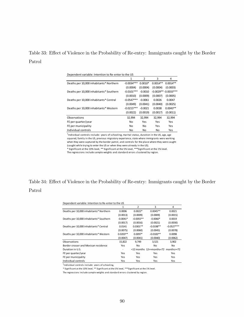
Table 33: E¤ect of Violence in the Probability of Re-entry: Immigrants caught by the Border

Patrol

Dependent variable: Intention to Re­enter to the US1 2 3 4

Deaths per 10,000 inhabitants* Northern ­0.0034*** 0.0010* 0.0014** 0.0014**(0.0004) (0.0004) (0.0004) (0.0003)

Deaths per 10,000 inhabitants* Southern ­0.0101*** ­0.0010 ­0.0029** ­0.0033***(0.0010) (0.0009) (0.0007) (0.0005)

Deaths per 10,000 inhabitants* Central ­0.0547*** ­0.0061 0.0026 0.0047(0.0049) (0.0041) (0.0040) (0.0025)

Deaths per 10,000 inhabitants* Western ­0.0215*** ­0.0021 0.0038 0.0043**(0.0022) (0.0019) (0.0017) (0.0011)

Observations 32,994 32,994 32,994 32,994FE per quarter/year No Yes Yes YesFE per municipality No No Yes YesIndividual controls No No No Yes

* Significant at the 10% level, ** Significant at the 5% level, ***Significant at the 1% level.The regressions include sample weights and standard errors clustered by region.

1Individual controls include:  years of schooling, marital status, duration in the US, age, agesquared, family in the US, previous migratory experience, state where immigrants were workingwhen they were captured by the border patrol, and controls for the place where they were caught(caught while trying to enter the US or when they were already in the US).

Table 34: E¤ect of Violence in the Probability of Re-entry: Immigrants caught by the Border

Patrol

Dependent variable: Intention to Re­enter to the US1 2 3 4

Deaths per 10,000 inhabitants* Northern 0.0006 0.0022* 0.0045** 0.0021(0.0013) (0.0009) (0.0009) (0.0015)

Deaths per 10,000 inhabitants* Southern ­0.0041* ­0.0055** ­0.0060* 0.0019(0.0017) (0.0016) (0.0021) (0.0030)

Deaths per 10,000 inhabitants* Central 0.0141 0.0301** ­0.0198** ­0.0527***(0.0075) (0.0060) (0.0045) (0.0078)

Deaths per 10,000 inhabitants* Western 0.0203** 0.0097* ­0.0183** 0.0098(0.0047) (0.0041) (0.0040) (0.0062)

Observations 15,822 9,749 3,521 3,902Border crosser and Mexican residence Yes No No NoDuration in U.S. ­ <12 months 12<=months<72 months>=72FE per quarter/year Yes Yes Yes YesFE per municipality Yes Yes Yes YesIndividual controls Yes Yes Yes Yes1Individual controls include:  years of schooling,* Significant at the 10% level, ** Significant at the 5% level, ***Significant at the 1% level.The regressions include sample weights and standard errors clustered by region.

90

four groups of workers.

The �rst one includes individuals caught crossing the border who report his country

of residence is Mexico, and four more categories according to their time in the US. The

results show that for individuals caught crossing the border and for individuals with less

than one year in the US the results are similar to the ones found in the previous section, an

increase in violence increases the out�ows from Western Mexico but decreases the out�ows

from Southern Mexico. However, when I analyze the behavior of individuals with more than

one year in the US the results change. For individuals from Central, Western and Southern

Mexico increases in violence are associated with a decrease in the probability to re-enter the

US. These results show that it is important to analyze the e¤ect of violence for individuals

with di¤erent durations in the US since the channels through which violence a¤ects them

and their decision to try to re-enter the US can change the longer they are in the United

States.

5.5.3 E¤ect of Violence on the Out�ows of Migrants: Analyzing the Di¤erences

by Region

Summarizing, the results show that the increase in violence increases the out�ows of migrants

from Western Mexico, but decreases the out�ows of migrants from Southern Mexico.

These �ndings highlight the importance of studying migration di¤erentiating individu-

als from di¤erent regions of Mexico. Migrants have di¤erent characteristics and respond

di¤erently to changes in social and economic conditions in Mexico15.

Western Mexico has been traditionally known as source of migrants; its migrants have

larger migration networks at destination, are more likely to have previous migratory experi-

ence, and are more likely to be sojourners. These characteristics might have contributed to

the increase in migration observed when violence increased.

15I analyze the migratory behavior of individuals aged 15-65 migrating to the U.S. to work or look for ajob. In the future I will analyze the e¤ect of violence on the migration behavior of other types of migrantslike wives, parents and children who migrate but not to work or look for a job.

91

Southern Mexico has been known as source of internal migration. However, since the 90�s

experienced important increases in their migration rates to the United States due to di¤erent

factors such as the introduction of recruiting programs for agricultural workers (H2A visas),

and the deterioration in the economic conditions of inhabitants of that region of Mexico.

When we look at the theoretical prediction of the e¤ect of violence, we �nd that violence

has an ambiguous e¤ect on migration out�ows.

The neoclassical theory of migration states that an individual will migrate if the earnings

at destination net of migration costs are higher than earnings at home. If the increase in

violence decreases expected earnings in Mexico the theory predicts that more individuals

will �nd it optimal to migrate to the United States.

Furthermore, violence could also increase migration costs. Migration costs have several

components, including monetary costs such as transportation costs, and non-monetary costs

such as the emotional cost of being away from family. An increase in violence could increase

transportation costs, for example, if migrants choose the route to the US that decreases the

probability of being targeted by criminal groups and not the shortest, fastest, or cheapest.

Moreover, violence could also increase the emotional cost of being away if individuals leave

their families back in Mexico in areas where they can be target of criminal groups, or decrease

it if individuals can migrate with their families to the US. Therefore, if migration costs

increase due to the increase in violence, fewer individuals will �nd it optimal to migrate.

One way to explain why the out�ows of workers from Western Mexico increased but the

out�ows of workers from Southern Mexico decreased would be if the social and economic

cost of violence is di¤erent for individuals from di¤erent regions of Mexico. For example, if

individuals from Western Mexico su¤er a large drop in expected earnings due to the increase

in violence relative to residents of Southern Mexico.

In order to test if the cost of violence is di¤erent for individuals from di¤erent regions

I use Mexico�s 2011 and 2012 National Survey on Victimization and Perceptions of Public

Safety (ENVIPE). This survey provides estimates of the number of crime victims, economic

losses due to crime, as well as perceptions of public safety at the national and sub-national

92

levels. Since the decision to migrate is determined by expected earnings, it is important to

analyze not only the actual cost of violence for those who were victims of a crime, but also

the perception of individuals with respect to the probability of becoming a victim. Violence

impacts individuals or businesses, decreases investment, consumption as well as individuals�

earnings, job performance or the ability to keep a job.

Table 35 shows regression results. Columns 1 and 2 show the perception of individuals

with respect to public safety. The dependent variable is a dummy variable equal to 1 if

the individual feels unsafe in their own neighborhood (municipality). Columns 3 and 4

measure the actual economic loss due to crime and the dependent variable is the logarithm

of the real loss. The independent variables included in all regressions are dummy variables

for regions of Mexico, urban, suburban and rural areas, sex and year of the survey. I also

include number of homicides by municipality committed between 2007 and the survey year

per 10,000 inhabitants, age and years of schooling. Finally, I include a dummy variable

for individuals in the labor force, unemployed as well as dummy variables for type of job

(farm workers, factory workers, owners/employers, individuals who work without pay and

self-employed). Regressions shown in columns 2, 4 and 6 also include the annual crime rate

by municipality per 10,000 inhabitants.16 All regressions include �xed e¤ects by year.

The results show that individuals from Western Mexico feel more unsafe in their own

municipality and have higher losses due to crime. Mexicans from Western states are 6.7

percentage points more likely to feel insecure in their neighborhood than individuals from

Southern Mexico, followed by individuals from Central (5.4 percent) and Northern Mexico

(3.2 percent).

Similarly, individuals fromWestern Mexico have the highest economic losses due to crime.

They had loses 11.66 log points higher than individuals from Southern Mexico followed by

individuals from Northern Mexico (9.68 log points).

These results can help us to understand why an increase in violence only increased the

out�ows of workers from Western Mexico. They have the highest drops in expected earnings

16The crime rate is the number of reported crimes. The types of crimes include property crimes, personalcrimes, kidnapping, and sexual crimes among others.

93

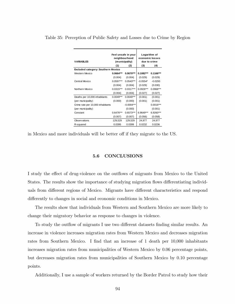
Table 35: Perception of Public Safety and Losses due to Crime by Region

VARIABLES(1) (2) (3) (4) (5) (6)

Excluded category: Southern MexicoWestern Mexico 0.0664*** 0.0670*** 0.1082*** 0.1166*** 0.0015 0.0035

(0.004) (0.004) (0.029) (0.029) (0.004) (0.004)Central Mexico 0.0597*** 0.0543*** ­0.0554* ­0.0293 ­0.0645*** ­0.0645***

(0.004) (0.004) (0.029) (0.030) (0.004) (0.004)Northern Mexico 0.0315*** 0.0317*** 0.0926*** 0.0968*** ­0.0172*** ­0.0141**

(0.004) (0.004) (0.027) (0.027) (0.005) (0.006)Deaths per 10,000 inhabitants 0.0049*** 0.0049*** (0.001) (0.001) 0.0018*** 0.0018***(per municipality) (0.000) (0.000) (0.001) (0.001) (0.000) (0.000)Crime rate per 10,000 inhabitants ­0.0004*** 0.0016*** ­0.0001**(per municipality) (0.000) (0.001) (0.000)Constant 0.6476*** 0.6573*** 6.9649*** 6.9260*** 0.2213*** 0.2201***

(0.007) (0.007) (0.056) (0.058) (0.009) (0.009)Observations 129,529 129,529 24,977 24,977 111,208 111,208R­squared 0.0395 0.0399 0.0232 0.0236 0.0496 0.0497

Logarithm ofeconomic losses

due to crime

Stopped traveling byland to other states

due to violence alongroads

Feel unsafe in yourneighbourhood(municipality)

in Mexico and more individuals will be better o¤ if they migrate to the US.

5.6 CONCLUSIONS

I study the e¤ect of drug-violence on the out�ows of migrants from Mexico to the United

States. The results show the importance of studying migration �ows di¤erentiating individ-

uals from di¤erent regions of Mexico. Migrants have di¤erent characteristics and respond

di¤erently to changes in social and economic conditions in Mexico.

The results show that individuals from Western and Southern Mexico are more likely to

change their migratory behavior as response to changes in violence.

To study the out�ow of migrants I use two di¤erent datasets �nding similar results. An

increase in violence increases migration rates from Western Mexico and decreases migration

rates from Southern Mexico. I �nd that an increase of 1 death per 10,000 inhabitants

increases migration rates from municipalities of Western Mexico by 0.06 percentage points,

but decreases migration rates from municipalities of Southern Mexico by 0.10 percentage

points.

Additionally, I use a sample of workers returned by the Border Patrol to study how their

94

probability to re-enter the US di¤ers for individuals from municipalities with di¤erent levels

of violence. The results show that an increase of 1 death per 10,000 inhabitants increases the

probability to re-enter for individuals from Western Mexico by 0.43 percentage points, but

decreases the probability to re-enter for migrants from Southern Mexico by 0.33 percentage

points.

The neoclassical theory of migration states that an individual will migrate if the earnings

at destination net of migration costs are higher than earnings at home. If the increase in

violence decreases expected earnings in Mexico the theory predicts that more individuals

will �nd it optimal to migrate. However, if violence increases migration costs the prediction

is that fewer individuals will migrate.

One way to explain why the out�ows of workers from Western Mexico increased but the

out�ows of workers from Southern Mexico decreased would be if the social and economic

cost of violence is di¤erent for individuals from di¤erent regions of Mexico. For example, if

individuals from Western Mexico su¤er a large drop in expected earnings due to the increase

in violence relative to residents of Southern Mexico.

I test if the decrease in earnings is di¤erent for di¤erent regions of Mexico using Mexico�s

2011 and 2012 National Survey on Victimization and Perceptions of Public Safety. The

results show that individuals fromWestern Mexico feel more unsafe in their own municipality

and have higher losses due to crime. Therefore, the large decrease in their expected earnings

in Mexico could have contributed to the increase in the out�ows of workers from that region

of Mexico.

As future extension I would like to analyze if the e¤ects found in this chapter are similar

for men and women and how duration in the United States change individuals�behavior.

Additionally it would be interesting to analyze the e¤ect of violence on the migratory be-

havior of other types of migrants like wives, parents and children who migrate but not to

work or look for a job.

95

6.0 APPENDIX

6.1 APPENDIX TO CHAPTER 1

6.1.1 Calculating probability of success crossing the border

According to the United States Border Patrol, during the �scal year of 2011 there were

340,252 apprehensions. Estimates from the GAO1 show that during that period of time the

estimated known illegal entries were 533,571. These numbers imply that the Border Patrol

has an apprehension rate of 36 percent. Carrion-Flores (2006) uses the Mexican Migration

Project, a survey conducted in Mexican towns of Western Mexico historically characterized

as important major suppliers of Mexican immigrants to estimate an apprehension rate of 32

percent.

Additionally, it has been documented that an important number of migrants try to re-

enter after being apprehended by the Border Patrol. Data from the EMIF shows that on

average 72 percent of the immigrants caught reported intention to re-enter the US within a

few days.

Using this information I calculate the probability of crossing successfully. I assume I

have 100 migrants trying to enter the US, 64 percent of them are successful in their �rst

try, and 36 will be caught by the Border Patrol. Of those 36 caught, 72 percent will try

to re-enter (26), and 10 will go back to Mexico. If 26 migrants try to re-enter, 17 of them

will be successful in their second try (64 percent of them), 9 will be apprehended, and 6 of

1United States Government Accountability O¢ ce. Report GAO-13-25 �BORDER PATROL: Key El-ements of New Strategic Plan Not Yet in Place to Inform Border Security Status and Resource Needs�,December 2012

96

the apprehended will try to re-enter (72 percent). The numbers of migrants who return to

Mexico are 10 after the �rst try and 3 after the second try. If 6 individuals try to enter a

third time, 4 will be successful (64 percent of them), 2 will be apprehended, and 1 will return

to Mexico. Therefore, the probability of successfully crossing the border is estimated to be

86 percent. I estimate an average number of crossings of the individuals who were caught

at least one time while entering the US of 1.33 times. This number is in line with the 1.24

estimated using the data of individuals returned by the Border Patrol from the EMIF.

97

6.2 APPENDIX TO CHAPTER 2

6.2.1 Graphs

98

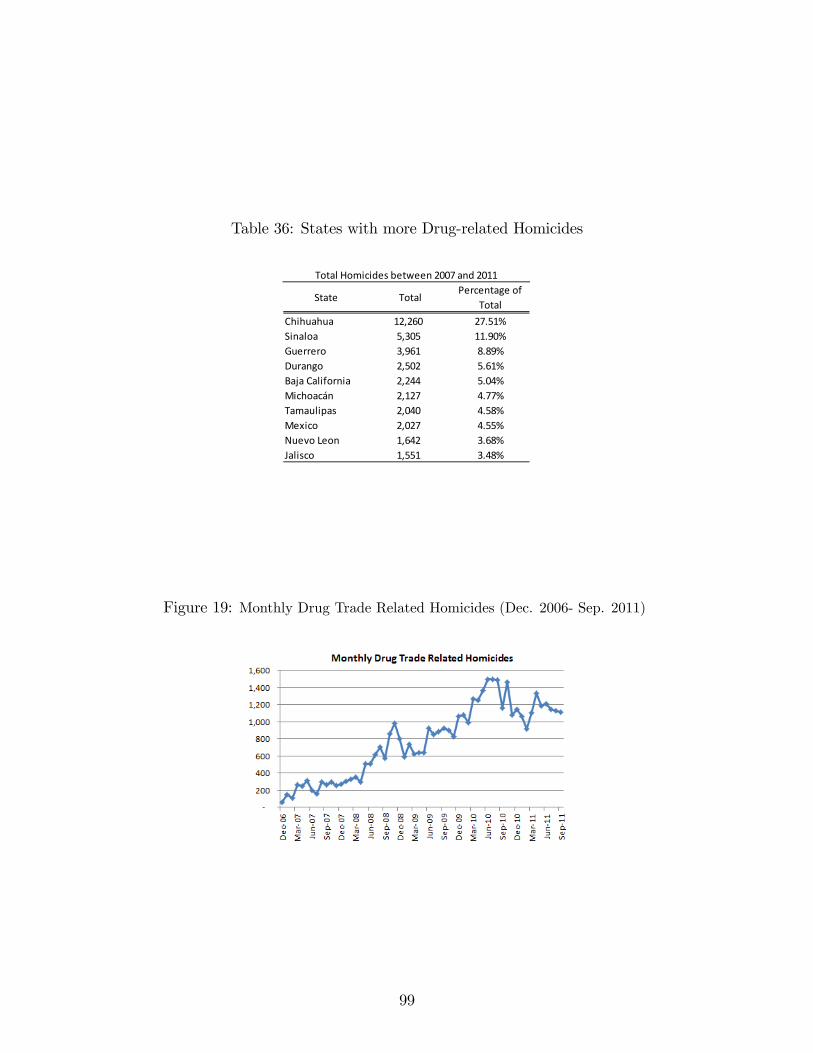
Table 36: States with more Drug-related Homicides

Chihuahua 12,260 27.51%Sinaloa 5,305 11.90%Guerrero 3,961 8.89%Durango 2,502 5.61%Baja California 2,244 5.04%Michoacán 2,127 4.77%Tamaulipas 2,040 4.58%Mexico 2,027 4.55%Nuevo Leon 1,642 3.68%Jalisco 1,551 3.48%

Total Homicides between 2007 and 2011

State TotalPercentage of

Total

Figure 19: Monthly Drug Trade Related Homicides (Dec. 2006- Sep. 2011)

99

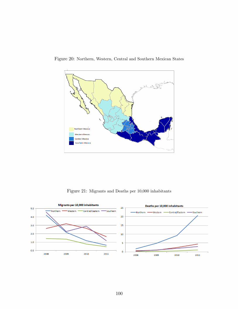
Figure 20: Northern, Western, Central and Southern Mexican States

Figure 21: Migrants and Deaths per 10,000 inhabitants

100

BIBLIOGRAPHY

[1] Adelman, I. and Taylor, E. (1990). �Is Structural Adjustment with a Human FacePossible? The Case of Mexico.�Journal of Development Studies. 26: 387�407.

[2] Arceo-Gómez, E. (2012). "Drug-Related Violence, Forced Migration and the ChangingFace Of Mexican Immigrants in the United States." Working Paper, Centro de Investi-gación y Docencia Económicas.

[3] Becker, A. (2009, March 20), �New Migrant Class Flees Mexican Drug War,�Center forInvestigative Reporting, http://cironline.org/reports/new-migrant-class-�ees-mexican-drug-war-2265

[4] Blanch�ower, D. and Oswald A. (1998)., �What Makes an Entrepreneur?.�Journal ofLabor Economics, 16, pp. 26-60.

[5] Borjas, G. J. (1985). �Assimilation, Changes in Cohort Quality, and the Earnings ofImmigrants.�Journal of Labor Economics, Vol. 3, No. 4, pp. 463-489.

[6] Borjas, G.J. (1996). �The Earnings of Mexican Immigrants in the United States.�Jour-nal of Development Economics 51(1):69-98.

[7] Borjas, G.J. (1999). Heaven�s Door: Immigration Policy and the American Economy.Princeton, NJ: Princeton University Press.

[8] Borjas G. (1987). "Self-selection and the earnings of immigrants". American EconomicReview, 77 (4): 531-553.

[9] Borjas, G. J. (1989). "Immigrant and Emigrant Earnings: A Longitudinal Study," Eco-nomic Inquiry 27 , 21-37.

[10] Borjas, G. J. (1994). �The economics of immigration�. Journal of Economic Literature,32, 1667�1717.

[11] Borjas G. and Bratsberg B. (1996). "Who leaves? The outmigration of the foreign-born".Review of Economics and Statistics, 87 (1): 165-176.

[12] Brownell, P. B. (2010). "Wages Di¤erences Between Temporary and Permanent Immi-grants." International Migration Review, 44: 593�614.

101

[13] Carletto, C., Davis B., Stampini M., Trento S., and Zezza A., (2004). �Internal Mobilityand Interantional Migration in Albania.�FAO ESA Working Paper No. 04-13, 2004.

[14] Chiquiar, D. and G.H. Hanson (2005). �International Migration, Self-Selection, and theDistribution of Wages: Evidence fromMexico and the United States. Journal of PoliticalEconomy, 113(2): 239-281

[15] Chiswick, B.R. (2000) �Are Immigrants Favorably Self-Selected?�Pp. 61-76 inMigrationTheory: Talking Across Disciplines, edited by C.B. Brettell and J.F Holli�eld. New York:Routledge.

[16] Dell M. (2012). "Tra¢ cking Networks and the Mexican Drug War�, Working Paper,MIT.

[17] Dinerman, I.R. (1982). �Migrants and Stay-at-Homes: A Comparative study of ruralMigration from Michoacan, Mexico.�Center for US-Mexican Studies, Monograph SeriesNo. 5. U.C. San Diego.

[18] Djajic, S. and Melbourne, R. (1988). �A General Equilibrium Model of Guest-workerMigration." Journal of International Economics 25:335-351.

[19] Duleep H. (1994) "Social Security and the Emigration of Immigrants." Social SecurityBulletin, Vol. 57, No. 1, 1994.

[20] Duleep H. and Dowhan D. (2008) "Adding Immigrants to Microsimulation Models"Social Security Bulletin, Vol. 68, No. 1, 2008.

[21] Dustmann, C., (1995). �Savings behavior of migrant workers: A Life-Cycle Analysis.�Zeitschrift fFur Wirtschafts- und Sozialwissenschaften 115, 511�533.

[22] Dustmann, C., (1997). �Return Migration, Uncertainty and Precautionary Savings.�Journal of Development Economics, 52, 295�316.

[23] Dustmann C. and Weiss Y. (2007). "Regurn Migration: Theory and Empirical Evidencefrom the UK". British Journal of Industrial Relations, June 2007 pp. 236-256.

[24] Dustmann and Kirchkamp (2002). �The Optimal Migration Duration and EconomicActivities after Re-Migration.�Journal of Development Economics, 67, 351-372, 2002.

[25] Evans, David S. and Leighton, Linda S.,(1989). �Some Empirical Aspects of Entrepre-neurship.�American Economic Review, Vol. 79, Issue 3, p. 519-535 1989.

[26] Feliciano, C. (2005). �Educational selectivity in US Immigration: How do immigrantscompare to those left behind.�Demography, Vol.42, No. 1, pp. 131-152.

[27] Fernández-Huertas, J. (2011). �New Evidence on Emigrant Selection�. The Review ofEconomics and Statistics 93:72-96.

102

[28] Funkhouser, E., (1992). �Remittances from international migration: a comparison of ElSalvador and Nicaragua.�Review of Economics and Statistics 77, 137�146.

[29] Germenji, E., and Swinnen J. (2004). �Impact of remittances on household-based farmsin rural Albania.�Paper presented at the International Conference on New Perspectiveson Albanian Migration and Development, Albania, 2004.

[30] Gitter , S., Gitter R., Southgate, D. (2008). �The Impact of Return Migration to Mex-ico.�Estudios Economicos, Vol. 23, No. 1, January-June 2008.

[31] Hanson, G. H., (2006). �Illegal Migration from Mexico to the United States.�NBERWorking Paper 12141.

[32] Hill, J. K. (1987). �Immigrant decisions concerning the duration of stay and migrationfrequency,�Journal of Development Economics, 25, 221�234.

[33] Holtz-Eakin, D., Joulfaian D., and Rosen H., (1994). �Sticking it Out: EntrepreneurialSurvival and Liquidity Constraints.� Journal of Political Economy, Vol. 102 (1), pp.53-75.

[34] Hurst E. and Lusardi A. (2004). �Liquidity Constraints, Household Wealth, and Entre-preneurship.� Journal of Political Economy, University of Chicago Press, vol. 112(2),pages 319-347.

[35] Ibarraran, P. and D. Lubotsky (2007) . �Mexican Immigration and Self-Selection: NewEvidence from the 2000 Mexican Census�in Mexican Immigration to the United States(eds. G.J. Borjas) University of Chicago Press (for NBER).

[36] Ilahi, N.(1999). �Return Migration and Occupational change.�Review of DevelopmentEconomics, 3,170-86.

[37] Jasso, G. and M.R. Rosenzweig (1982). "Estimating the emigration rates of legal im-migrants using administrative and survey data: the 1971 cohort of immigrants to theUnited States.." Demography, 19: 279-290.

[38] Jasso, G. and M.R. Rosenzweig (1990). "Self-Selection and the Earnings of Immigrants:Comment." American Economic Review 80:298-304.

[39] Kaestner, R. and Malamud, O., (2010). "Self-Selection and International Migration:New Evidence from Mexico," NBER Working Papers 15765, National Bureau of Eco-nomic Research.

[40] King, R., and Vullnetari J., (2003). �Migration and Development in Albania.�Devel-opment Research Centre on Migration, Globalization and Poverty, Sussex Centre forMigration Research, Working Paper C5, 2003.

103

[41] Kule, D., Mancellari, A., Papapanagos H., Qirici S., and Sanfey P., (2002). �The Causesand Consequences of Albanian Emigration during Transition: Evidence from Micro-data.�International Migration Review, 36.1, pp. 229-239.

[42] Lee, E.S. (1966). �A Theory of Migration.�Demography 3:47-57.

[43] Lindstrom, D. P. (1996). �Economic Opportunity in Mexico and Return Migration fromthe United States�, Demography, Vol. 33, no. 3, 357-374.

[44] López, G. (1986). �La Casa Dividida: Un Estudio de Caso Sobre Migación a EstadosUnidos en un Pueblo Michoacano.�Zamora, Michoacán: El Colegio de Michoacán.

[45] Lucas, R., and Stark O. (1985) �Motivation to Remit: Evidence from Botswana,�Jour-nal of Political Economy, Vol. 93, No. 5, 901-918.

[46] Massey, D.S. (1987).�Understanding Mexican Migration to the United States.�Ameri-can Journal of Sociology 92:1372-403.

[47] Massey, D.S. (1999).�Why Does Immigration Occur? A Theoretical Synthesis.�Pp. 34-52 in Handbook of International Migration, edited by C. Hirschman, P. Kasinitz, andJ. DeWind. New York: Rusell Sage Foundation.

[48] Massey, D. S., Arango, J., Graeme, H., Kouaoci A., Pellegrino A. and Taylor E. (1993),�Theories of International Migration: A Review and Appraisal.�Population and Devel-opment Review, Vol. 19, No. 4, pp. 699�751.

[49] McCornick, B. and Wahba, J. (2001): �Overseas work experience, savings and entre-preneurship amongst return migrants to LDCs.�Scottish Journal of Political Economy,Special Conference Issue, 48: 164-78.

[50] Mesnard, A. (2004). �Temporary Migration and Capital Market Imperfections.�OxfordEconomic Papers, 2004, 56.2, pp. 242-262.

[51] McKenzie, D. and Rapaport H. (2010). "Self-Selection Patterns in Mexico-USMigration:The Role of Immigration Networks." The Review of Economics and Statistics. MITPress, vol. 92(4), pages 811-821.

[52] Murillo Castaño, G. (1988). �E¤ects of Emigration and Return on Sending Countries:The Case of Columbia.� International Migration Today. Ed. C. Stahl. Geneva: UN-ESCO.

[53] Murphy, R. (2000). �Return Migration, Entrepreneurship and Local State Corporatismin Rural China: The Experience of Two Counties in South Jiangxi.�Journal of Con-temporary China, 2000, 9.24, pp. 231-4.

[54] Nickell J.K. (2013). "Immigration: The New � and Rich � Immigrants from Mexico:How Their Money is Changing Texas." January. 14, 2013. Time Magazine.

104

http://nation.time.com/2013/01/14/the-new-and-rich-immigrants-from-mexico-how-their-money-is-changing-texas/

[55] Orozco S. (2011). �Labor Market E¤ects of Immigration Policies� Working Paper,University of Pittsburgh.

[56] Orrenius, P. and Zavodny, M. (2005). "Self-Selection Among Undocumented Immigrantsfrom Mexico." Journal of Development Economics 78: 215-240.

[57] Passel, J.S. (2006). �Estimates of the Size and Characteristics of the UndocumentedPopulation.�Pew Hispanic Center.

[58] Passel, J., Cohn D., and Gonzalez-Barrera, A. (2012). �Net Migration from Mexico Fallsto Zero� and Perhaps Less�. Pew Hispanic Center.

[59] Piracha and Vadean (2010). �Return Migration and Occupational Choice: Evidencefrom Albania�. World Development, Volume 38, Issue 8, August 2010, Pages 1141�1155.

[60] Portes, A. and R.G. Rumbaut. (1996). �Immigrant America: A Portrait�. Berkeley:University of California Press.

[61] Rios V., and Shirk D. (2011). �Drug Violence in Mexico: Data and Analysis Through2010�. Trans-Border Institute.

[62] Roy, A.D. (1951). �Some Thoughts on the Distribution of Earnings.�Oxford EconomicPapers 3:135-46.

[63] Schulkin P. (2012). "The Revolving Door Deportations of Criminal Illegal Immigrants."Center for Immigration Studies.

[64] Schultz, T.P. (1984). �The Schooling and Health of Children of US Immigrants andNatives.�Research in Population Economics 5:251-88.

[65] Sjaastad, L. (1962). "The Costs and Returns of Human Migration." Journal of PoliticalEconomy, Vol. 70, No. 5, Part 2, pp. 80-93.

[66] Stark, O. (1991) The Migration of Labor. London: Basil Blackwell.

[67] Taylor E. (1996). �Development Strategy, Employment and Migration: Insights fromModels.�Organization for Economic Co-operation and Development [OECD], 1996. 207p. (Development Centre Seminars).

[68] Taylor, J.E. (1999), �The New Economics of Labor Migration and the Role of Remit-tances�, International Migration, Vol. 37(1), pp. 63-86.

[69] Taylor, J.E., Mora, J., Adams, R. and Lopez-Feldman, A. (2005). �Remittances, In-equality and Poverty: Evidence from Rural Mexico�. University of California, Davis,Working Paper No. 05-003.

105

[70] United States Government Accountability O¢ ce (2012). "Report GAO-13-25 �BorderPatrol: Key Elements of New Strategic Plan Not Yet in Place to Inform Border SecurityStatus and Resource Needs�, December 2012

[71] Wahba and Zenou (2009). �Out of Sight, Out of Mind: Migration, Entrepreneurshipand Social Capital.�CEPR Discussion Papers 7552, C.E.P.R. Discussion Papers.

[72] Warren, R. and Peck, J.M. (1980). "Foreign born emigration from the United States".Demography, 17: 71-84.

[73] Woodru¤, C. (2006). �Mexican Microenterprise Investment and Employment: The Roleof Remittances.�Working Paper.

[74] Woodru¤, C., and Zenteno, R. (2004). �Remmittances and Mircroenterprises in Mex-ico.�University of California at San Diego. Working Paper 2004.

[75] Woodru¤, C., and Zenteno, R. (2007). �Migration networks and microenterprises inMexico.�Journal of Development Economics, 82, 509�528.

106