soluciones especiales de sistemas...
TRANSCRIPT
UNIVERSIDAD DE BUENOS AIRESFacultad de Ciencias Exactas y Naturales
Departamento de Matematica
Soluciones Especiales de Sistemas A-hipergeometricos
Tesis presentada para optar al tıtulo deDoctor de la Universidad de Buenos Aires
en el area Ciencias Matematicas
Federico Nicolas Martınez
Directora de tesis: Dra. Alicia DickensteinConsejera de estudios: Dra. Alicia Dickenstein
Buenos Aires, 2011

2

La mentira tiene patas cortas..., pero a veces usa zancos.
3

4
Unas palabras...
La principal responsable de que esta tesis empezara y terminara sos vos, Alicia. Estoy muyagradecido de haberte conocido y trabajado con vos. Sos una gran persona y me voy a lle-var un recuerdo lleno de carino y momentos divertidos (y aburridos tambien, no me gusta lainvestigacion, pero no es culpa tuya, jajaja).
Ademas de Alicia y yo, Laura Matusevich y Eduardo Cattani son autores del contenidomatematico que aca aparece. Agradezco a Laura su hospitalidad cuando estuve en USA y eltiempo que trabajamos juntos. Eduardo me ayudo primero regalandome un libro y despuesaportando su tiempo y sus conocimientos para poder terminar lo que faltaba.
Compartı estos anos con muchas personas lindas del departamento de Matematica:Los chicos de la oficina son los mejores que podrıa haber tenido. No solo pasamos un
monton de ratos carentes de todo tipo de trabajo (y por lo tanto maravillosos) sino que ademasme bancaron cuando ya no querıa saber nada con la facultad y estaba mas ocupado con elteatro y, despues, con el compost y los delirios existenciales. Mechi, la companera ideal, todoslos dıas con muchas sonrisas y (otras) galletitas. Nico, companero de viajes y conversacionesinteresantes, cuando seas decano vuelvo a la facu. Juampi, el santafesino mas copado queconocı y conocere, nunca dejo que me fuera rengo. Fran, sos mas simpatico de lo que pareces,gracias por ayudarme con el Latex, sin vos esta tesis no tendrıa dibujitos. Fer, una presenciasilenciosa y llena de significado, te deseo lo mejor cuando te vuelvas a tus lejanos pagos.Marina, las moscas volveran. Los chicos de al lado, siempre con buena onda: Pablito, Juanjo,Alexandra. Nico Capitelli solo estuvo unos meses, pero fueron de los mejores.
Gente del futbol, gracias. Sin esa brevısima hora semanal, todo hubiera sido (mucho) maspesado: Lea dp, el Colo, el Vendra, Santi L., Ferchu, Andres, Santi M., Manu, Ariel S., Damian,Agustın, Dani C., Patu, Ariel P., Lea L., Nino, Adrian, Lucas, Roman y faltan jugadores....
Gente de almuerzos, pasillos, cumpleanos y docencia compartida, tambien gracias (muchosde los del futbol tambien van aca): Rela, Dano, Vicky, Maggie, Coty, Caro C., Caro M., Guille,Seba, Sandra, Marcela F., Marıa Laura N., Lea Z., Fede Q... aca tambien me voy a olvidar dealguno...
Las chicas de secretarıa y biblioteca por sus sonrisas: Sole, Sandra, Marıa Angelica,Gisela. Tambien me acuerdo de Edemia y Carlos, por la simpatıa matinal.
Muchos alumnos me dejaron recuerdos de los mas lindos aca en la facu. No se si les ensenedemasiado, pero ellos a mı, un monton. Me acuerdo de Antonella (gracias por el mate :), deMauro, de Alejandro y, obviamente, de Libertad.
Mi tıa Mirta me abrio los brazos con mucho amor cuando me vine a vivir a Buenos Aires,nunca se lo terminare de agradecer. Tambien mi primo Pablito me banco un monton en estaaventura portena.
5

6
Y, por supuesto, como no agradecer a Marıa Cecilia. Sos mucho mas que una companera,mi amor y mi alegrıa. Nos vinimos aca para esto y ahora... a donde vamos?
7
Abstract
The A-hypergeometric systems of differential equations introduced by Gelfand, Kapranovand Zelevinsky are a generalization of a broad class of differential equations in the complexdomain, incorporating analytical, algebro-geometrical and combinatorial tools. In this work,we study two different types of special (holomorphic multivalued) A-hypergeometric func-tions, that is, two types of special solutions of A-hypergeometric systems. On one hand, weintroduce a proper notion of Nilsson solutions for the space of formal solutions of irregular A-hypergeometric systems, we explore the dimension of this space and convergence issues. Thesecond problem addressed in the thesis is the characterization of algebraic A-hypergeometricfunctions admitting a Laurent series expansion, for regular configurations that are Cayley con-figurations of two planar configurations, in terms of appropriate multidimensional residues.
Keywords: A-hypergeometric, irregular D-module, Nilsson series, multidimensional residue,algebraic function.
Resumen
Los sistemas de ecuaciones diferenciales A-hipergeometricos introducidos por Gelfand,Kapranov y Zelevinsky constituyen una generalizacion de una amplia clase de ecuaciones difer-enciales en el campo complejo, incorporando herramientas analıticas, algebro-geometricas ycombinatorias. En este trabajo se estudian dos tipos distintos de funciones (holomorfas mul-tivaluadas) A-hipergeometricas especiales, es decir dos tipos de soluciones especiales de sis-temas A-hipergeometricos. Por un lado, se introduce una nocion apropiada de soluciones deNilsson para el espacio de soluciones formales de sistemas A-hipergeometricos irregulares yse estudia la dimension de este espacio ası como la convergencia. El segundo problema abor-dado en la tesis ha sido la caracterizacion de funciones A-hipergeometricas algebraicas queadmitan un desarrollo como series de Laurent, para configuraciones regulares A, que seanconfiguraciones de Cayley de dos configuraciones planas, en terminos de apropiados residuosmultidimensionales.
Palabras clave: A-hipergeometrico, D-modulo, series de Nilsson, residuo multidimensional,funcion algebraica.

8
Introduction
The solutions of the Gauss hypergeometric equation are described by means of the Gauss hy-pergeometric series. Their formal study begun, precisely, with Gauss and it is still an activearea of research, involving many areas of mathematics such as complex analysis, number the-ory, combinatorics, mathematical physics, etc.
In the early 90’s, Gel’fand, Kapranov and Zelevinsky studied several differential equationsof hypergeometric type (Gauss, Horn, Lauricella, etc.) and introduced a common frameworkfor all of them (see [GKZ89], [GKZ88],[GKZ90]), namely, the A-hypergeometric systems (orGKZ-hypergeometric systems), whose solutions are called A-hypergeometric functions. Theirwork involves D-modules, toric varieties, combinatorics and other tools. The information of thesystem is codified in a integer matrix A (that can also be thought as a configuration of integerpoints), and a complex vector β. The A-hypergeometric system with parameter β is denotedby HA(β).
In this thesis we study two special kinds of solutions ofA-hypergeometric systems: Nilssonsolutions of irregular A-hypergeometric systems, in chapters 3 and 4, and algebraic Laurentsolutions of Cayley configurations, in chapters 5 and 6.
In 2000, Saito, Sturmfels and Takayama gave a Grobner Basis reformulation of the GKZtheory. Our way to deal with A-hypergeometric systems is based on their work. We overviewsome of their ideas and results in chapter 1. In chapter 2 we explain two combinatorial toolsthat we strongly use in the rest of the work: Gale dual and coherent mixed subdivisions. Theother fundamental tool from combinatorics is that of coherent triangulations that is treated inSection 1.4.2.
In the first part of our work, we study solutions of irregular A-hypergeometric systems.For an integer matrix A and a complex parameter β, the system HA(β) is a holonomic D-ideal [Ado94, GKZ89]. It is also known that HA(β) is regular holonomic if and only if theQ-rowspan of the matrix A contains the vector (1, . . . , 1). The if direction was proved by Hottain his work on equivariant D-modules [Hot91]; Saito, Sturmfels and Takayama gave a partialconverse in [SST00, Theorem 2.4.11], assuming that the parameter β is generic.
The Frobenius method is a symbolic procedure for solving a linear ordinary differentialequation in a neighborhood of a regular singular point. The solutions are represented as con-vergent logarithmic Puiseux series that belong to the Nilsson class. In the multivariate case, theSaito, Sturmfels and Takayama method, called the canonical series algorithm, applied to a reg-ular holonomic left D-ideal, yields a basis of the solution space [SST00, Chapter 2]. The basiselements belong to an explicitly described Nilsson ring, and are therefore called Nilsson series,or Nilsson solutions. Each Nilsson ring is constructed using a weight vector; the choice ofweight vector is a way of determining the common domain of convergence of the correspond-
9

10
ing solutions. The canonical series procedure requires a regular holonomic input; although onecan run this algorithm on holonomic left D-ideals that have irregular singularities, there is noguarantee that the output series converge, or even that the correct number of basis elements willbe produced.
In Section 3.1, we extend the notion of Nilsson solution to general A-hypergeometric sys-tems. For arbitrary A and β, we denote by Nw(HA(β)) the space of Nilsson solutions of thesystem HA(β). In order to obtain the elements of Nw(HA(β)), we introduce, in section 3.2, anapplication ρ of homogenization that goes from Nw(HA(β)) to an associated regular system.
For generic parameters, we calculate in Section 3.3 the dimension of Nw(HA(β)) in com-binatorial terms, and construct an explicit basis. Ohara and Takayama [OT09] showed that themethod of canonical series for a weight vector which is a perturbation of (1, . . . , 1) produces abasis for the solution space of HA(β) consisting of (convergent) Nilsson series that contain nologarithms. We extend their results and give in section 4.2 a criteria to decide which elementsof the constructed basis of Nw(HA(β)) converge, for arbitrary weight vectors w.
In order to produce a basis of solutions for HA(β) when β is not generic, logarithmic seriescannot be avoided, even in the regular case. We study them in section 3.4. Dealing withlogarithmic solutions of HA(β) poses technical challenges that we resolve here, allowing us tolift the genericity hypotheses from the results of Ohara and Takayama: running the canonicalseries algorithm on HA(β) with weight vector (a perturbation of) (1, . . . , 1) always producesa basis of (convergent) Nilsson solutions of HA(β), if the cone spanned by the columns of Ais strongly convex (i.e., the cone contains no lines). This is done in section 4.1. On the otherhand, formal solutions of irregular hypergeometric systems that are not Nilsson series need tobe considered, even in one variable (see, for instance, [Cop34].)
Finally, in section 3.5, we extend the proof of Saito, Sturmfels and Takayama of the con-verse of Hotta’s regularity theorem mentioned above, assuming that the cone over the columnsofA is strongly convex. This gives an alternative proof to a result given by Schulze and Walther.
In fact, a different strategy to show that a D-ideal is not regular holonomic is to prove thatit has slopes. The analytic slopes of a D-module were introduced in the work of Mebkhout[Meb89], while an algebraic version was given by Laurent [Lau87]. These authors have shownthat the analytic and algebraic slopes of a D-module along a hypersurface agree [LM99]. Froma computational perspective, Assi, Castro–Jimenez and Granger gave a Grobner basis algorithmto find algebraic slopes [ACG96]. There has been an effort to compute the (algebraic) slopes ofHA(β) along a coordinate hypersurface. In the cases d = 1 and n − d = 1, these slopes weredetermined by Castro–Jimenez and Takayama [CT03], and Hartillo–Hermoso [Har03, Har05].More generally, Schulze and Walther [SW08] have calculated the slopes of HA(β) under thestrongly convex assumption. The fact that slopes of HA(β) always exist when the vector(1, . . . , 1) does not belong to the rowspan of A, implies that HA(β) has irregular singularities.Thus, [SW08, Corollary 3.16] gives a converse for Hotta’s regularity theorem in the stronglyconvex case. Our proof is done by extending ideas of Saito, Sturmfels and Takayama, where themain technical obstacle to overcome is the potential existence of logarithmic hypergeometricseries.
Further insight into the solutions of hypergeometric system comes from the analytic ap-proach taken up by Castro–Jimenez and Fernandez–Fernandez [CF11, Fer10], who studied theGevrey filtration on the irregularity complex of an A-hypergeometric system. Since formal se-ries solutions of irregular systems need not converge, a study of the Gevrey filtration provides
11
information on how far such series are from convergence.In the second part of our work, we study in chapters 5 and 6, Laurent solutions of a regular
A-hypergeometric system where the configuration A is a Cayley configuration of k configura-tion in dimension k. A configuration A is Cayley if given A1, . . . , As configurations in Zr
A = {e1} × A1 ∪ · · · ∪ {es} × As.
If we consider polynomials with these supports
fi(t) =
|Ai|∑j=1
xjtaj , i = 1, . . . , r,
generically in the coefficients xj , the common zeros of fi i = 1, . . . , r are finite and simple.Then the local Grothendieck residue
Resf1,...,fr,ξ(tm) =
ξm
JTf (ξ)
is well-defined. If V is the set of common zeros of the polynomials fi, then the global residue
Resmf =∑ξ∈V
Resf1,...,fr,ξ(tm)
is an algebraic A-hypergeometric function with homogeneity (−1, . . . ,−1,−m).The study of univariate algebraic hypergeometric functions is a classical subject. Beukers
and Heckman [BH89] gave an explicit classification of all algebraic univariate hypergeometricseries (see also [Rod]). There exists a small number of general results on algebraicity of A-hypergeometric functions in the multivariate case (that is, for configurations of codimensiongreater than one). A recent work of Beukers ([Beu10]), characterizes those configurationsA forwhich exists generic parameters such that all solutions are algebraic. Our study is based on thedetermination and explicitation of algebraic A-hypergeometric functions for certain resonantvalues of the parameters (for which there also exists logarithmic solutions and the monodromyis not finite) in terms of multidimensional residues.
The existence of non-trivial rational A-hypergeometric functions imposes severe combi-natorial constraints on the configuration A. In [CDS01] it was conjectured that A needs tocarry an essential Cayley structure. This was elucidated in several articles (see, eg., [CDS01],[CDD99],[CDR11]), in connection with the structure of the fullA-determinant [GKZ94], whichdefines the singular locus of HA(β) for any β.
It follows from those papers that in the case of the Cayley configurations of k configurationsin dimension k that we consider, there are no non-trivial rational solutions. Our results showthat the algebraicity of A-hypergeometric Laurent series is also imposed by purely combinato-rial conditions. We next explain more in detail our statements.
As a generalization of [CDD99], we work with the case of two polynomials f1, f2 in thevariables t1, t2. We study the possible minimal regions, that is, subsets of {1, . . . , |A1|+ |A2|}indexing the variables that appear in the denominators of the Laurent solutions associated tothe configuration A and to homogeneity parameters (−1,−1,−m) lying in the Euler-Jacobi

12
cone of A (see Definition 5.15.) We establish in Section 5.2 a precise relation between infiniteminimal regions and interior points of the Minkowski sum of the convex hulls of A1 y A2.
The common roots of f1, f2 can be obtained from mixed cells of the coherent mixed sub-division of the configuration, following work of Huber and Sturmfels [HS95]). To each mixedcell σ in a coherent mixed subdivision of the Minkowski sum of the given configurations, onecan associate as many roots of f1, f2 as the normalized volume of σ. We define in Section 6.1the residue Resσf relative to σ adding the local residues over the roots corresponding to σ.
Theorem 6.2.2, our main result in Section 6.2, gives an explicit way of writing each residueResσf as a linear combination of the canonical solutions associated to minimal regions cor-responding to interior points of the Minkowski sum of the convex hulls of A1 y A2 that arevertices of σ. The coefficients of this linear combination are combinatorially defined. In Theo-rem 6.3.1 of Section 6.3, we give a complete description of algebraic LaurentA-hypergeometricfunctions in terms of residues, in case |A1| + |A2| = 6 and no Ai has an interior point. In thelast section, we highlight the complications that arise in more general situations and we stategeneral conjectures which would extend our results.
Contents
1 Regular A-hypergeometric systems 151.1 From the classical equation to A-hypergeometric systems . . . . . . . . . . . . 15
1.1.1 Solving equation 1.1 via the Frobenius method . . . . . . . . . . . . . 151.1.2 Introducing homogeneities in the classical hypergeometric equation . . 171.1.3 The GKZ hypergeometric systems . . . . . . . . . . . . . . . . . . . . 18
1.2 Holonomic systems . . . . . . . . . . . . . . . . . . . . . . . . . . . . . . . . 181.3 Canonical solutions . . . . . . . . . . . . . . . . . . . . . . . . . . . . . . . . 201.4 Hypergeometric regular ideals . . . . . . . . . . . . . . . . . . . . . . . . . . 25
1.4.1 Invariants of the configuration A . . . . . . . . . . . . . . . . . . . . . 251.4.2 The fake initial ideal of HA(β) . . . . . . . . . . . . . . . . . . . . . . 261.4.3 Hypergeometric canonical series . . . . . . . . . . . . . . . . . . . . . 291.4.4 Gamma series for generic parameters . . . . . . . . . . . . . . . . . . 30
2 Tools from combinatorics 332.1 Secondary Fan . . . . . . . . . . . . . . . . . . . . . . . . . . . . . . . . . . 332.2 Coherent mixed subdivisions . . . . . . . . . . . . . . . . . . . . . . . . . . . 35
3 Formal Nilsson solutions 473.1 Initial ideals and formal Nilsson series . . . . . . . . . . . . . . . . . . . . . . 473.2 Homogenization of formal Nilsson solutions of HA(β) . . . . . . . . . . . . . 503.3 Hypergeometric Nilsson series for generic parameters . . . . . . . . . . . . . . 563.4 Logarithm-free Nilsson series . . . . . . . . . . . . . . . . . . . . . . . . . . . 603.5 The irregularity of HA(β) via its Nilsson solutions . . . . . . . . . . . . . . . 62
4 Convergence of hypergeometric Nilsson series 674.1 General parameters . . . . . . . . . . . . . . . . . . . . . . . . . . . . . . . . 674.2 Generic parameters . . . . . . . . . . . . . . . . . . . . . . . . . . . . . . . . 70
5 Laurent A-hypergeometric solutions and residues 755.1 A-hypergeometric Laurent series . . . . . . . . . . . . . . . . . . . . . . . . . 755.2 Minimal regions and Minkowski sum . . . . . . . . . . . . . . . . . . . . . . 795.3 Residues and Cayley configurations . . . . . . . . . . . . . . . . . . . . . . . 835.4 A-hypergeometric solutions associated to a vertex . . . . . . . . . . . . . . . . 85
13

14 CONTENTS
5.4.1 The Gelfond-Khovanskii method for calculating residues . . . . . . . . 855.4.2 Laurent polynomial solutions . . . . . . . . . . . . . . . . . . . . . . 86
5.5 A necessary condition for the algebraicity . . . . . . . . . . . . . . . . . . . . 87
6 Algebraic A-hypergeometric solutions and residues 916.1 Coherent mixed subdivisions and residues . . . . . . . . . . . . . . . . . . . . 916.2 Algebraic solutions as residues . . . . . . . . . . . . . . . . . . . . . . . . . . 936.3 The case n = 6 . . . . . . . . . . . . . . . . . . . . . . . . . . . . . . . . . . 95
6.3.1 The case r = s = 3 . . . . . . . . . . . . . . . . . . . . . . . . . . . . 966.3.2 The case r = 2, s = 4 . . . . . . . . . . . . . . . . . . . . . . . . . . 101
6.4 General conjectures . . . . . . . . . . . . . . . . . . . . . . . . . . . . . . . . 103

Chapter 1
Regular A-hypergeometric systems
A-hypergeometric systems are a generalization of classical hypergeometric equations and leadus to consider partial differential equations in Cn instead of ordinary differential equationsin C. The theory of D-modules gives the appropriated tools to deal with them, because thecoefficients of these partial differential equations are polynomials in Cn. Saito, Sturmfels andTakayama presented in [SST00] an algorithm to solve regular systems using Grobner bases inthe Weyl algebra. Moreover, they showed that in the case of an hypergeometric D-module,due to its combinatorial nature, their methods are more accurate. Our objective in Chapter3 is to solve irregular hypergeometric systems, but inspired on the techniques in [SST00], sowe introduce in this chapter the basics on D-modules, the method of Saito, Sturmfels andTakayama and the combinatorial aspects of the A-hypergeometric systems.
1.1 From the classical equation toA-hypergeometric systems
In this informal section, we present an overview of the “evolution” of hypergeometric functions.After introducing the Gauss hypergeometric series we present the A-hypergeometric seriesrelated to it and the A-hypergeometric system associated as well as some examples.
The Gauss hypergeometric equation
[x(x− 1)d2
dx2+ (c− x(a+ b+ 1))
d
dx− ab] • f = 0 (1.1)
where a, b, c are complex parameters has been widely studied since Gauss. Note that the sin-gular points of this equations are x = 0, x = 1 and x = ∞. Its importance in mathematics aswell as in physics relies in the fact that any equation with three regular singular points can bewritten in this form. We will explain in Section 1.3 the notion of regularity in one and morevariables with more detail, but for the purpose of this introductory section we will describe themanner to obtain the solutions of the equation (1.1) around its singular points.
1.1.1 Solving equation 1.1 via the Frobenius method
We will operate in a pure algebraic way to obtain formal solutions around the singular pointx = 0. The general procedure to obtain the solutions in this case will be discussed when wedeal with regularity in Chapter 1.
15

16 CHAPTER 1. REGULAR A-HYPERGEOMETRIC SYSTEMS
Suppose we are looking for a (multivalued) solution of the shape:
f = xs ·∞∑k=0
ckxk (1.2)
that is a power series around x = 0 times xs with s ∈ C (choose an appropriated branch of thelogarithm).
Regard the differential operator in (1.1) as and element P in the Weyl algebra D = k〈x, ∂〉.Thus P can be written as
P = [x(x− 1)∂2 − (a+ b+ 1)x∂ + c∂ − ab]. (1.3)
Applying it to both sides of (1.2) we have
xP • f =∞∑k=0
ck(s+ k)(s+ k + c− 1)xs+k −∞∑k=0
ck(s+ k + a)(s+ k + b)xs+k+1 = 0
and we obtain the following recurrence relations for the coefficients ck:
s(s+ c− 1) = 0,
(s+ k + 1)(s+ k + c)ck+1 − (s+ k + a)(s+ k + b)ck = 0, k = 0, 1, 2, . . .
Assume c0 = 1. Once that the exponent s is chosen by means of the first equation, we canobtain the coefficients ck through the second one. If s = 0 then
ck =(a)k(bk)
(1)k(c)k
where
(a)k =Γ(a+ k)
Γ(a)
is the Pochhammer symbol. If, on the other hand, s = 1− c then
ck =(a+ 1− c)k(b+ 1− c)k
(1)k(2− c)k.
Note that in both cases we need c /∈ Z to obtain ck for all k = 0, 1, 2, . . .. We have obtainedtwo formal solutions to (1.1) around x = 0:
F (a, b, c;x) :=∞∑k=0
(a)k(bk)
(1)k(c)kxk (1.4)
andx1−c.F (a+ 1− c, b+ a− c, 2− c;x). (1.5)
The function F (a, b, c;x) is also denoted by 2F1(a, b, c;x) and it is called Gauss Hypergeomet-ric Function with parameters (a, b, c).
1.1. FROM THE CLASSICAL EQUATION TO A-HYPERGEOMETRIC SYSTEMS 17
1.1.2 Introducing homogeneities in the classical hypergeometric equation
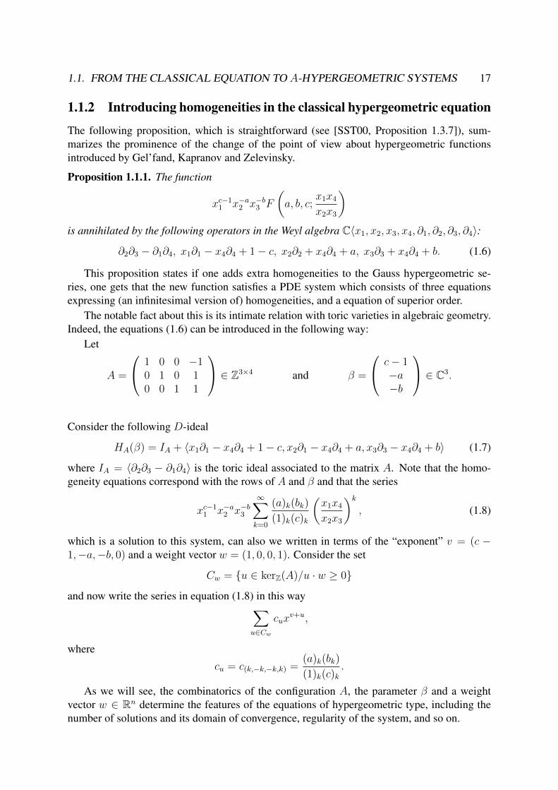
The following proposition, which is straightforward (see [SST00, Proposition 1.3.7]), sum-marizes the prominence of the change of the point of view about hypergeometric functionsintroduced by Gel’fand, Kapranov and Zelevinsky.
Proposition 1.1.1. The function
xc−11 x−a2 x−b3 F
(a, b, c;
x1x4
x2x3
)is annihilated by the following operators in the Weyl algebra C〈x1, x2, x3, x4, ∂1, ∂2, ∂3, ∂4〉:
∂2∂3 − ∂1∂4, x1∂1 − x4∂4 + 1− c, x2∂2 + x4∂4 + a, x3∂3 + x4∂4 + b. (1.6)
This proposition states if one adds extra homogeneities to the Gauss hypergeometric se-ries, one gets that the new function satisfies a PDE system which consists of three equationsexpressing (an infinitesimal version of) homogeneities, and a equation of superior order.
The notable fact about this is its intimate relation with toric varieties in algebraic geometry.Indeed, the equations (1.6) can be introduced in the following way:
Let
A =
1 0 0 −10 1 0 10 0 1 1
∈ Z3×4 and β =
c− 1−a−b
∈ C3.
Consider the following D-ideal
HA(β) = IA + 〈x1∂1 − x4∂4 + 1− c, x2∂1 − x4∂4 + a, x3∂3 − x4∂4 + b〉 (1.7)
where IA = 〈∂2∂3 − ∂1∂4〉 is the toric ideal associated to the matrix A. Note that the homo-geneity equations correspond with the rows of A and β and that the series
xc−11 x−a2 x−b3
∞∑k=0
(a)k(bk)
(1)k(c)k
(x1x4
x2x3
)k, (1.8)
which is a solution to this system, can also we written in terms of the “exponent” v = (c −1,−a,−b, 0) and a weight vector w = (1, 0, 0, 1). Consider the set
Cw = {u ∈ kerZ(A)/u · w ≥ 0}and now write the series in equation (1.8) in this way∑
u∈Cwcux
v+u,
where
cu = c(k,−k,−k,k) =(a)k(bk)
(1)k(c)k.
As we will see, the combinatorics of the configuration A, the parameter β and a weightvector w ∈ Rn determine the features of the equations of hypergeometric type, including thenumber of solutions and its domain of convergence, regularity of the system, and so on.
18 CHAPTER 1. REGULAR A-HYPERGEOMETRIC SYSTEMS
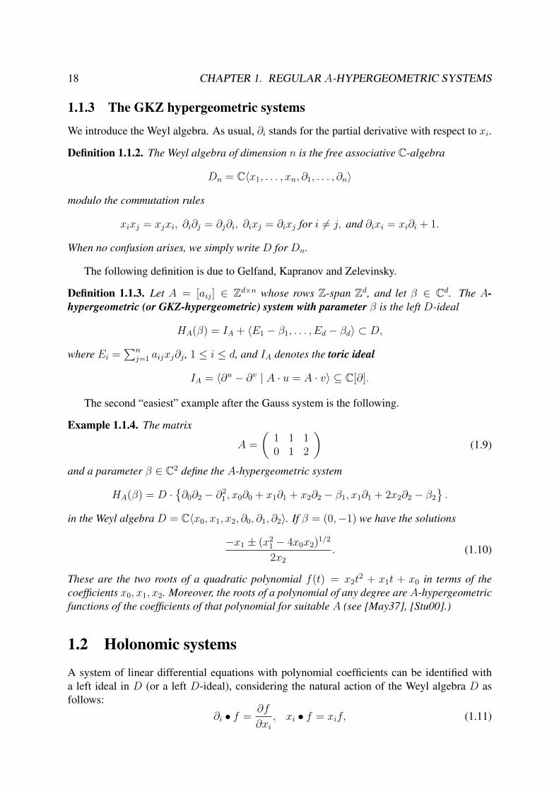
1.1.3 The GKZ hypergeometric systems
We introduce the Weyl algebra. As usual, ∂i stands for the partial derivative with respect to xi.
Definition 1.1.2. The Weyl algebra of dimension n is the free associative C-algebra
Dn = C〈x1, . . . , xn, ∂1, . . . , ∂n〉
modulo the commutation rules
xixj = xjxi, ∂i∂j = ∂j∂i, ∂ixj = ∂ixj for i 6= j, and ∂ixi = xi∂i + 1.
When no confusion arises, we simply write D for Dn.
The following definition is due to Gelfand, Kapranov and Zelevinsky.
Definition 1.1.3. Let A = [aij] ∈ Zd×n whose rows Z-span Zd, and let β ∈ Cd. The A-hypergeometric (or GKZ-hypergeometric) system with parameter β is the left D-ideal
HA(β) = IA + 〈E1 − β1, . . . , Ed − βd〉 ⊂ D,
where Ei =∑n
j=1 aijxj∂j , 1 ≤ i ≤ d, and IA denotes the toric ideal
IA = 〈∂u − ∂v | A · u = A · v〉 ⊆ C[∂].
The second “easiest” example after the Gauss system is the following.
Example 1.1.4. The matrix
A =
(1 1 10 1 2
)(1.9)
and a parameter β ∈ C2 define the A-hypergeometric system
HA(β) = D ·{∂0∂2 − ∂2
1 , x0∂0 + x1∂1 + x2∂2 − β1, x1∂1 + 2x2∂2 − β2
}.
in the Weyl algebra D = C〈x0, x1, x2, ∂0, ∂1, ∂2〉. If β = (0,−1) we have the solutions
−x1 ± (x21 − 4x0x2)1/2
2x2
. (1.10)
These are the two roots of a quadratic polynomial f(t) = x2t2 + x1t + x0 in terms of the
coefficients x0, x1, x2. Moreover, the roots of a polynomial of any degree are A-hypergeometricfunctions of the coefficients of that polynomial for suitable A (see [May37], [Stu00].)
1.2 Holonomic systems
A system of linear differential equations with polynomial coefficients can be identified witha left ideal in D (or a left D-ideal), considering the natural action of the Weyl algebra D asfollows:
∂i • f =∂f
∂xi, xi • f = xif, (1.11)
1.2. HOLONOMIC SYSTEMS 19
where f may belong to many differentD-modules, such as formal power series C[[x1, . . . , xn]],holomorphic functions O(U) on an open subset U of Cn, etc. Thus, we say that the element fis a solution of the (left) ideal I of D if p • f = 0 for all p ∈ I .
Any element p of D has a unique expression of the form
p =∑u,v∈Nn
cuvxu∂v
where cuv = 0 for all but finitely many pairs (u, v). Associated with D we consider thecommutative polynomial ring R = C[x1, . . . , xn, ξ1, . . . , ξn]. Given any non-zero p ∈ D letν(p) := max{|v| : cuv 6= 0 for some u ∈ Nn} be the order of p and set
σ(p) :=∑
u∈Nn,|v|=ν(p)
cuvxuξv ∈ R.
The polynomial σ(p) is called the (principal) symbol of the differential operator p.
Definition 1.2.1. Given a left ideal I ⊂ D, its characteristic variety is the affine variety in C2n
defined by the characteristic ideal ch(I) := 〈σ(p) : p ∈ I〉 ⊂ R.
Definition 1.2.2. A left ideal I ⊂ D is called holonomic if and only if its characteristic idealhas (Krull) dimension n. The holonomic rank of I is the dimension of the following vectorspace over the field of rational functions C(x):
rank(I) := dimC(x)
(C(x)[ξ]
(C(x)[ξ] · ch(I))
).
Holonomic systems have the following nice property ([SST00, Proposition 1.4.9]).
Proposition 1.2.3. If I is a holonomic D-ideal, then rank(I) is finite.
Definition 1.2.4. Let I ⊂ D be a left ideal and V(ch(I)) ⊂ C2n its characteristic variety. Thesingular locus Sing(I) is defined as the Zariski closure of the projection on Cn
x of
V(ch(I))− {ξ1 = · · · = ξn = 0}.
The following theorem ([SST00, Theorem 1.4.19]) is a result of Kashiwara that relates theholonomic rank of a D-ideal I to its solution space.
Theorem 1.2.5. Let I be a holonomic ideal and U a simply connected domain in Cn−Sing(I).Consider the system of differential equations I • f = 0. Then the dimension of the complexvector space of holomorphic solutions is equal to rank(I).
Example 1.2.6. The prototypical example of a holonomic D-ideal is the principal D-idealdefined by a linear ordinary (this is n = 1) differential equation of order m:
I = D · {am(x)∂m + am−1(x)∂m−1 + · · ·+ a0(x)},
where the ai’s are polynomials in x and am 6= 0. Here ch(I) = 〈am(x)ξm〉, hence I isholonomic with rank(I) = m. The singular locus is the zero set {x ∈ C : am(x) = 0} ofthe polynomial am. Theorem 1.2.5 reduces in this case to the classical theorem of existence ofsolutions around non-singular points.
20 CHAPTER 1. REGULAR A-HYPERGEOMETRIC SYSTEMS
1.3 Canonical solutions
In [SST00], Saito, Sturmfels and Takayama presented a method to obtain series solutions forregular holonomic D-ideals. In this section we briefly describe this method.
The key idea is to obtain the “first part” of the solutions solving the “first part” of theequations and then produce an actual solution, in an analogous way to the Frobenius method inone variable. For this, we define the initial of a D-ideal.
Definition 1.3.1. For an element p =∑
u,v cuvxu∂v in the Weyl algebra D, and a vector w ∈
Rn, we define in(−w,w)(p) to be the sum of the terms of p in which the inner product (u, v) ·(−w,w) achieves its maximum. If I is a left D-ideal, we define
in(−w,w)(I) = 〈in(−w,w)(p) | p ∈ I〉 ⊂ D.
For a holonomic ideal, we have the following result which is Theorem 2.2.1 in [SST00].
Theorem 1.3.2. Let I be a holonomic D-ideal and w ∈ Rn. The initial D-ideal in(−w,w)(I) isalso holonomic and
rank(in(−w,w)(I)) ≤ rank(I). (1.12)
Remark 1.3.3. The vector w ∈ Rn is called weight vector in [SST00]. We will ask strongerconditions to w in Chapters 3 and 4 when the ideal is not regular, so we will reserve the termweight vector for that case. See Definition 3.1.1.
The following step is to look at the shape of the solutions so that the expression “first part”makes sense. This will be possible if we assume that the system is regular.
We first introduce the notion of regularity for an ordinary differential equation. Considerthe equation
am(x)∂m
∂xmf(x) + am−1(x)
∂m−1
∂xm−1f(x) + · · ·+ a1(x)
∂
∂xf(x) + a0(x) = 0 (1.13)
where the functions ai(x) are holomorphic in an open set U ⊂ C and let x0 ∈ U such thatam(x0) = 0. We say that x0 is a regular singular point of the equation (1.13) if the functions
bi(x) :=ai(x)
am(x)
have at worst a pole of order m− i at x0.The following theorem is classical and its proof can be found in [CL55].
Theorem 1.3.4. Let x0 be a regular singular point of (1.13). Then the following statementshold:
1. The vector space of multivalued holomorphic functions in a sufficiently small punctureddisk {0 < |x−x0| < ε}, which are solutions of (1.13), has dimensionm and is generatedby functions of the form
(x− x0)λ(ln(x− x0)j)f(x),
where λ ∈ C, j ∈ Z, 0 ≤ j ≤ m − 1, f(x) is holomorphic in the disk {|x − x0| < ε}and f(x0) 6= 0.

1.3. CANONICAL SOLUTIONS 21
2. If the series
g(x) = (x− x0)λk∑j=0
( ∞∑l=0
clxl
)ln(x− x0)j,
where λ, cl ∈ C and k ∈ N, formally satisfies the equation (1.13) then there exists apunctured disk {0 < |x − x0| < ε} such that g(x) defines a multivalued holomorphicfunction in there.
We now present a definition of regularity of an arbitrary D-module as given in [SST00].The definition involves complicated tools which we not discuss in this thesis, and we include itfor the sake of completeness, being the properties of regular D-modules what is important forus. Denote by DX the sheaf of algebraic differential operators on X = Cn.
Definition 1.3.5. Let I be a holonomic ideal in the Weyl algebraD. Let C be a smooth curve inX = Cn and j : C → Cn an embedding. A holonomic DX-module DX/DXI is called regularholonomic when Lkj∗(DX/DXI) is regular holonomic on a smooth compactificationC for anysuch curve C and for all k = 0,−1, . . . ,−n+1. WhenDX/DXI is regular holonomic, we callI regular holonomic. Here Lkj∗ is the k-th derived functor of j∗.
The following result is known and appears in [SST00] as Theorem 2.4.12 and Corollary2.4.14.
Theorem 1.3.6. Let I be a regular holonomic D-ideal. Assume that the singular locus of I iscontained in an algebraic hypersurface that is a normal crossing divisor locally at the origin.Then there exist vectors α1, . . . , αm in Cn such that any multivalued holomorphic solution of Ion {∏n
i=1 xi 6= 0} near the origin has a series expression in the ring
C[[x1, . . . , xn]][xα1 , . . . , xαm , log(x1), . . . , log(xn)].
These series converge around the origin, and they are polynomials in log(xi) of degree at mostrank(I)− 1.
The hypotheses of Theorem 1.3.6 mean that if s(x) is the polynomial defining Sing(I), thenit can be written as
s(x) = xa ·(
1 +∑u∈B
cuxu
)(1.14)
where cu ∈ C∗, B ⊂ Nn and a ∈ Zn. In a general case, we can always find a change ofvariables that leads to a expression like (1.14) and it turns out that the shape of the solutionsprovided by Theorem 1.3.6 is governed by the convex geometry of the singular locus.
In fact, assume that I is a regular holonomic D-ideal and suppose that
s(x) =l∑
k=1
cmkxmk
with mk ∈ Nn, k = 1, . . . , l is the defining polynomial of a hypersurface that contains Sing(I).Applying a multiplicative change of coordinates:
xj = yv1j
1 yv2j
2 . . . yvnjn for j = 1, . . . , n (1.15)

22 CHAPTER 1. REGULAR A-HYPERGEOMETRIC SYSTEMS
we obtain
s(x1, . . . , xn) = yV ·m1
(1 +
l∑k=2
cmkyV ·(mk−m1)
)(1.16)
where V is the matrix whose rows are the vectors (vi1, . . . , vin). How do we choose V so thatthe condition (1.14) is satisfied, that is V · (mk −m1) ≥ 0 for all k = 2, . . . , l?
Suppose that the monomial xq occurs in s. Consider the Newton polytope New(s) of s.Then q is a vertex of New(s). Take a cone C which has its vertex at q and contains New(s)with generators γ1, . . . , γn ∈ Zn. We can assume that the determinant of (γ1, . . . , γn) = ±1.The n× n matrix U = (γ1, . . . , γn) is invertible over Z and let V = (vij) be its inverse matrix.This implies that the row vectors of V span the polar cone C∗, that is, the cone of all vectorw ∈ Rn such that 〈w, γi〉 ≥ 0 for i = 1, . . . , n.
Then m1 = q and mk = q +∑n
i=1 λikγi with λik non-negative integers and the conditions
required are satisfied, because
V · (mk −m1) =n∑i=1
λikV · γi = (u1, . . . , un)
is a non-negative integer vector, for k = 2, . . . , l.Then we have the following result, [SST00, Corollary 2.4.16].
Theorem 1.3.7. The regular holonomic D-ideal I has a fundamental set of solutions on 0 <|xui | � 1 each of which is represented by a series in
N = C[[xu1
, . . . , xun
]][xα1 , . . . , xαm , log(x1), . . . , log(xn)]. (1.17)
where α1, . . . , αm are suitable vectors in Cn
The ring N gives the appropriated context to work with initial of series solutions. In fact, avector w ∈ Rn defines a partial term order ≤ on N as follows:
xa log(x)b ≤ xc log(x)d ⇔ Re(a · w) ≤ Re(c · w). (1.18)
If g =∑
a,b cabxa log(x)b is a non zero element of N , then the set of real parts {Re(a · w) |
cab 6= 0 for some b} achieves a (finite) minimum, denoted by µ(g). Moreover, the subseries ofg consisting of terms cabxa log(x)b such cab 6= 0 and Re(a · w) = µ(g) is finite by [SST00,Proposition 2.5.2]. We call this finite initial sum the initial series of g with respect to w and wedenote it by inw(g).
Remark 1.3.8. The ring N is not closed under differentiation in general. These and othertechnical reasons are dealt carefully in [SST00, Section 2.5]. Here we just explain the basicsto reach to a general understanding of the Saito, Sturmfels and Takayama method.
By means of the following theorem ([SST00, Theorem 2.5.5]) it is possible to identify whatwe called the “first part” of a series solution.
Theorem 1.3.9. If f ∈ N is a solution to I then inw(f) is a solution to in(−w,w)(I).

1.3. CANONICAL SOLUTIONS 23
The term order (1.18) can be refined by the lexicographic term order. We denote this refine-ment by ≺w. Every element g of N has a unique initial monomial in≺w(g) with respect to ≺w.The following lemma is Lemma 2.5.6 and Proposition 2.5.7 in [SST00].
Lemma 1.3.10. Let g1, . . . , gk ∈ N .
1. If the initial monomials in≺w(g1), . . . , in≺w(gk) are distinct, then the initial series definedby inw(g1), . . . , inw(gk) are C-linearly independent.
2. If the initial series inw(g1), . . . , inw(gk) are C-linearly independent, then g1, . . . , gk are C-linearly independent.
3. If g1, . . . , gk are C-linearly independent, there exists a k× k complex matrix (λij) such thatthe initial series of ψi =
∑kj=1 λijgj for i = 1, . . . , k are C-linearly independent.
The following theorem (Theorem 2.5.1 in [SST00]) states a notable fact about regular holo-nomic systems.
Theorem 1.3.11. Let I be a regular holonomic D-ideal and w ∈ Rn. Then
rank(I) = rank(in(−w,w)(I)). (1.19)
Remark 1.3.12. The proof of Theorem 1.3.11 is not difficult. First, note that by Theorem 1.3.2we just need to prove that rank(I) ≤ rank(in(−w,w)(I)). The crucial fact is that a fundamentalset of solutions to I (with rank(I) many elements) on an open ball U ⊂ Cn can be representedby series in N , by Theorem 1.3.7. Then apply Theorem 1.3.9 and Lemma 1.3.10 to obtain thedesired result. We want to emphasize that this argument cannot be replicated in the non-regularcase, because we do not have that nice description of the solutions.
The shape of the solutions of a regular holonomic ideal can be more accurate than Theorem1.3.7. We first introduce the important notion of exponent.
Definition 1.3.13. A vector v ∈ C is an exponent of a D-ideal I with respect to w ∈ Rn if xv
is a solution of in(−w,w)(I).
Remark 1.3.14. For a holonomic ideal, the set of exponents is finite because of Proposition1.2.3 and Theorem 1.3.2.
The vectors ui in Theorem 1.3.7 can also be better understood by means of the convexgeometry of the ideal I .
Definition 1.3.15. Let I be a regular holonomic D-ideal and w ∈ Rn generic. The Grobnercone of I containing the vector w is defined by
Cw(I) ={w′ ∈ Rn : in(−w,w)(I) = in(−w′,w′)(I)
}(1.20)
Cw(I) is a union of open convex polyhedral cones in Rn, since I is a regular holonomicD-ideal and w is generic. The polar cone of Cw(I) is, by definition, the set Cw(I)∗ of vectorsu ∈ Rn such that in(−w,w)(I) = in(−w′,w′)(I) implies u ·w′ ≥ 0. Since Cw(I) is n-dimensional,Cw(I)∗ is strongly convex, i.e., Cw(I)∗ contains no non-zero linear subpaces.
24 CHAPTER 1. REGULAR A-HYPERGEOMETRIC SYSTEMS
Consider the monoid consisting of all integer vectors
Cw(I)∗Z := Cw(I)∗ ∩ Zn
Write C[[Cw(I)∗Z]] for the ring of formal power series f =∑
u cuxu where u ∈ Cw(I)∗Z and
cu ∈ C∗. Since every non-constant term cuxu appearing in f satisfies w · u > 0, inw(f) is
well-defined for all f ∈ C[[Cw(I)∗Z]].Finally, we get to a full description of the solutions to a regular holonomic ideal (see Theo-
rems 2.5.12, 2.5.14 and 2.5.16 of [SST00]).
Theorem 1.3.16. Let I be a regular holonomicD-ideal andw ∈ Rn generic. Put r := rank(I).Then there exist a set C = {f1, . . . , fr} such that for i = 1, . . . , r:
1. fi is a solution to I .
2. in≺w(fi) = xai log(x)bi and in≺w(fi) 6= in≺w(fj) for i 6= j.
3. fi have the form xai · pi where ai is and exponent and pi is an element of the ring
C[[Cw(I)∗Z]][log(x1), . . . , log(xn)].
4. The degree of the logarithmic series pi of the previous item with respect to log(xk) is atmost rank(I)− 1 for every k = 1, . . . , n.
5. There exists a point x0 ∈ Cw(I) such that fi converges for x = (x1, . . . , xn) ∈ Cn
satisfying(− log |x1|, . . . ,− log |xn|) ∈ x0 + Cw(I).
The series fi, i = 1, . . . , r, of Theorem 1.3.16 are called the canonical (series) solutions forI with respect to ≺w. In Section 3.4 we will deal with logarithm free canonical series solutionsand in Section 5.1 with the particular case of canonical series which are Laurent (i.e., withinteger exponents).
Let {a1, . . . , ar} ⊂ Cn is the set of exponents of I . The ring
Nw(I) := C[[Cw(I)∗Z]][xa1 , . . . , xar , log(x1), . . . , log(xn)] (1.21)
is called the Nilsson ring with respect to w.Of course, we can consider an open set U ⊂ Cn and a (multivalued) holomorphic func-
tion in U that is a solution of the system HA(β) without regarding at any weight vector w,or consider the weight vector afterwards the holomorphic solution is defined. The followingdefinition clarifies this.
Definition 1.3.17. We say that a series
φ =∑
u∈supp(φ)
xupu(log(x)) (1.22)
that defines a (multivalued) holomorphic solution of the system HA(β) is a series solution ofHA(β) in the direction of w if the following conditions holds:
1. The pu are polynomials.
2. supp(φ) is contained in a strongly convex cone.
3. For every u ∈ supp(φ), 〈w, u〉 ≥ 0.
1.4. HYPERGEOMETRIC REGULAR IDEALS 25
1.4 Hypergeometric regular ideals
In this section we show how the techniques explained in Section 1.3 can be applied to the systemHA(β) in Definition 1.1.3. We analyze the combinatorial properties of the system HA(β) thatallow us to obtain the canonical series described in Theorem 1.3.16.
We first observe that A-hypergeometric systems are holonomic, which was proved first byGel’fand, Kapranov and Zelevinsky under hypothesis a) and b) below ([GKZ89]) and then byAdolphson (see [Ado94]) without assumptions on the configuration A.
Theorem 1.4.1. The D-ideal HA(β) is holonomic.
Hotta proved (see [Hot91]) that the A-hypergeometric systems are regular, provided thatthe associated toric variety is projective.
Theorem 1.4.2. If the vector (1, 1, . . . , 1) is in the Q-span of the row vectors of A, then HA(β)is regular holonomic for all β ∈ C.
We think of A, not just as a matrix, but also as the point configuration {a1, . . . , an} ⊂ Zd.We will assume the following conditions:
a) The vector (1, 1, . . . , 1) is in the Q-span of A.
b) The elements of A span the lattice Zd over Z.
Important combinatorial features were developed in [GKZ94] from A-hypergeometric sys-tems, such as Principal Determinants, Secondary Polytopes, Regular (coherent) triangulations,Secondary Fan, and more. Moreover, in [SST00] these structures are reviewed from a Commu-tative Algebra and Grobner Theory point of view. We discuss this and show that more accurateresults can be obtained if we assume that the parameter β is generic.
1.4.1 Invariants of the configuration A
The configuration A determines important properties of the system HA(β). Let conv(A) be theconvex hull of the columns a1, . . . , an of A. We consider a particular notion of volume (see[GKZ89]).
Definition 1.4.3. The normalized volume vol(A) is the Euclidean volume of conv(A) nor-malized so that the unit simplex in the lattice ZA has volume one. As we have assumed thatZA = Zd, the normalization is achieved by multiplying the Euclidean volume of conv(A) byd!.
The singularities of HA(β) are also made explicit by the structure of A.
Definition 1.4.4. Consider a generic polynomial with exponents in A:
f(t1, . . . , td) =n∑i=1
xitai .
The principal A-determinant is defined as the resultant
EA(f) = RA
(t1∂f
∂t1, . . . , td
∂f
∂td, f
). (1.23)
26 CHAPTER 1. REGULAR A-HYPERGEOMETRIC SYSTEMS
The following theorem summarizes the known results about the singularities and the calcu-lation of the holonomic rank of HA(β). The two first statements are due to Gel’fand, Kapranovand Zelevinsky [GKZ89] under assumptions a) and b) and to Adolphson [Ado94] in the gen-eral case. The third one is Theorem 3.5.1 in [SST00]. The if part of the last statement is due toGel’fand, Kapranov and Zelevinsky [GKZ89] and to Adolphson [Ado94]. The only if part wasproved by Matusevich, Miller and Walther [MMW05].
Theorem 1.4.5. Let HA(β) be an A-hypergeometric system.
1. The singular locus of the system is the zero set of the principal A-determinant:
Sing(A) = {EA = 0}.
2. For arbitrary A and generic β, rank(HA(β)) = vol(A).
3. For arbitrary A and β, rank(HA(β)) ≥ vol(A).
4. Given A, rank(HA(β)) = vol(A) for all β ∈ Cd if and only if the ideal IA is Cohen-Macaulay.
1.4.2 The fake initial ideal of HA(β)
In order to describe the series solutions with respect to w ∈ Rn of a regular holonomic D-idealI , we must first calculate the exponents, that is, the vectors v ∈ Cn such that xv is a solutionof in(−w,w)(I). In the case I = HA(β), an easy manipulable description of in(−w,w)(HA(β)) isknown when the parameters β are generic (see Theorem 3.1.3 in [SST00]).
Lemma 1.4.6. For β generic,
in(−w,w)(HA(β)) = inw(IA) + 〈E − β〉.
Definition 1.4.7. The idealinw(IA) + 〈E − β〉 (1.24)
is called the fake initial ideal of HA(β) and if xv is a solution to it, the vector v ∈ Cn is calleda fake exponent of HA(β) with respect to w.
Corollary 1.4.8. For the ideal HA(β), the set of exponents is included in the set of fake expo-nents.
Proof. This is clear because IA and E − β are both contained in HA(β).
Fake exponents are easier to manipulate than exponents (in the generic case they are thesame) and in general, they are useful to obtain the solutions of the system, as we will show.
Note that for v ∈ Cn to be an fake exponent it has to satisfy that xv is a solution of themonomial ideal inw(IA) ⊂ C[∂1, . . . , ∂n] and that for each row (ai1, . . . , ain) of A it holds:
n∑j=1
aijxj∂j(xv) = βix
v
1.4. HYPERGEOMETRIC REGULAR IDEALS 27
which turns into the following linear equations for v:
n∑j=1
aijvj = βi for i = 1, . . . , d.
That isA·v = β. So now we pay attention to the solutions of the ideal inw(IA) ⊂ C[∂1, . . . , ∂n].Note that if w is generic then inw(IA) is a monomial ideal.
A useful tool to find the solutions of a monomial ideal in C[∂] := C[∂1, . . . , ∂n] is that ofstandard pairs.
Definition 1.4.9. The set S(M) of standard pairs of the monomial ideal M ⊂ C[∂] is the set ofpairs (∂a, σ) where a ∈ Nn and σ is a subset of the index set {1, . . . , n} such that
1. ai = 0 if i ∈ σ.
2. {xv : v ∈ a+ Nσ} ∩M = ∅, where Nσ := {γ ∈ Nn : γl = 0, l /∈ σ}.
3. For each l /∈ σ, {xv : v ∈ a+ Nσ∪{l}} ∩M 6= ∅.
If the dimension ofM in C[∂] is d we call top-dimensional to an element (∂a, σ) ∈ S (M) suchthat |σ| = d. We denote T (M) the set of top-dimensional standard pairs of M .
Top-dimensional standard pairs are useful to describe the set top(M) of top-dimensionalcomponents of a monomial ideal M in C[∂], as Lemma 3.2.4 of [SST00] shows:
Lemma 1.4.10. Let M be a monomial ideal in C[∂].
top(M) =⋂
(∂a,σ)∈T (M)
〈∂ai+1i : i /∈ σ〉. (1.25)
As mentioned, we can describe the solutions of a monomial ideal in C[∂] by means of itsstandard pairs.
Proposition 1.4.11. For a monomial ideal M ⊂ C[∂], the solutions of the system of partialdifferential equations
∂uF = 0; ∂u ∈Mare functions of the form:
F (x) =∑
(∂a,σ)∈S(M)
xa · Fσ(x)
where the function Fσ(x) depends only on the variables xi, i ∈ σ.
For a better understanding of the fake initial ideal of HA(β), we introduce the notion ofsimplicial complex and subsequently, the notion of coherent triangulation of a convex polytope.
Definition 1.4.12. A family ∆ of subsets of {1, . . . , n} is called a simplicial complex when thefollowing two conditions are satisfied:
1. if σ ∈ ∆, then any subset of σ belongs to ∆.
28 CHAPTER 1. REGULAR A-HYPERGEOMETRIC SYSTEMS
2. if σ, τ ∈ ∆, then σ ∩ τ ∈ ∆.
Each subset in ∆ is called a face of the simplicial complex ∆.
There is a connection between simplicial complexes and monomial ideals.
Definition 1.4.13. The Stanley-Reisner ideal of ∆ is the ideal in C[∂1, . . . , ∂n] generated bymonomials
∏i∈σ ∂i where σ runs over all the subsets of {1, . . . , n} such that σ /∈ ∆.
Example 1.4.14.
∆ = {{1, 2, 3}, {2, 3, 4}, {1, 2}, {1, 3}, {2, 3}, {2, 4}, {3, 4}, {1}, {2}, {3}, {4}, ∅}is a simplicial complex on {1, 2, 3, 4} and its Stanley-Riesner ideal is 〈∂1∂4〉. Note that only list-ing top-dimensional faces (facets) is enough to determine a simplicial complex. For instance,in the above example we can write ∆ = {{1, 2, 3}, {2, 3, 4}}.Definition 1.4.15. A triangulation of a configurations of points A = {a1, . . . , an} in Rm is adecomposition of its convex hull conv(A) into simplices with vertices in A which are the (top)faces of a simplicial complex ∆.
A vector w ∈ Rn>0 induces a subdivision ∆w of the configuration A, by projecting the lower
hull of conv({(wi, ai) : i = 1, . . . , n}) onto conv(A) (see [Stu96, Chapter 8] for details). If wis generic, ∆w is a triangulation of A. Such subdivisions are usually called regular, but we usethe alternative term coherent.
We always write triangulations of A as simplicial complexes on {1, . . . , n}, but think ofthem geometrically: a simplex σ in such a triangulation corresponds to the geometric simplexconv({ai : i ∈ σ}). Example 1.4.14 gives a possible triangulation of the convex hull of fouraffinely independent points in R3.
There is a deep connection between initials of toric ideals, coherent triangulations and stan-dard pairs, explained in the following theorem due to Sturmfels (see [Stu96, Chapter 8]), thatwill help to understand the solutions of the A-hypergeometric systems.
Theorem 1.4.16. Let A be a homogeneous integer matrix and w ∈ Rn generic. Let M =inw(IA). The radical ideal
√M is the Stanley-Reisner ideal of the regular triangulation ∆w of
A defined by w and it can be described using the top-dimensional standard pairs of M in thefollowing way:
∆w = {σ : (∂a, σ) ∈ T (M) for some a}. (1.26)
Example 1.4.17. Let IA be the toric ideal associated to the matrix
A =
1 0 0 −10 1 0 10 0 1 1
.
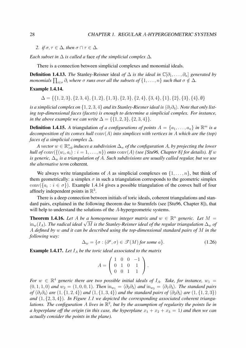
For w ∈ R4 generic there are two possible initial ideals of IA. Take, for instance, w1 =(0, 1, 1, 0) and w2 = (1, 0, 0, 1). Then inw1 = 〈∂2∂3〉 and inw2 = 〈∂1∂4〉. The standard pairsof 〈∂1∂4〉 are (1, {1, 2, 4}) and (1, {1, 3, 4}) and the standard pairs of 〈∂2∂3〉 are (1, {1, 2, 3})and (1, {2, 3, 4}). In Figure 1.1 we depicted the corresponding associated coherent triangu-lations. The configuration A lives in R2, but by the assumption of regularity the points lie ina hyperplane off the origin (in this case, the hyperplane x1 + x2 + x3 = 1) and then we canactually consider the points in the plane).

1.4. HYPERGEOMETRIC REGULAR IDEALS 29
b
1b
2
b3
b4
b
1b
2
b3
b4
∆w1 = {{1, 2, 4}, {1, 3, 4}} ∆w2 = {{1, 2, 3}, {2, 3, 4}}
Figure 1.1: The coherent triangulations of A for Example 1.4.17.
Example 1.4.18. Consider the configuration A defined by the matrix (1.9) in Example 1.1.4.The convex hull of A is the segment {1} × [0, 2] w [0, 2] and the toric ideal is given by IA =〈∂0∂2 − ∂2
1〉. The initial ideal 〈∂0∂2〉 gives the standard pairs (1, {0, 1}) and (1, {1, 2}) that is,the triangulation consisting in the simplices [0, 1] and [1, 2]. On the other hand, the initial ideal〈∂2
1〉 gives the standard pairs (1, {0, 2}) and (∂1, {0, 2}) and the corresponding triangulationis the whole segment [0, 2].
There is a better description of the fake initial ideal for β generic ([SST00, Theorem3.2.11]):
Theorem 1.4.19. Let w a generic vector in Rn. For generic parameters β, we have
in(−w,w)(HA(β)) = top(inw(IA)) + 〈E − β〉. (1.27)
Suppose that v is a fake exponent of HA(β) with respect to a generic vector w ∈ Rn, thenTheorem 1.4.19 together with Lemma 1.4.10 and Proposition 1.4.11 allow us to easily calculateit: pick (∂a, σ) ∈ T (inw(IA)) and set vi = ai for i /∈ σ. Then solve the system A · v whichis now a d × d invertible system, because σ is actually a simplex in the triangulation ∆w. Wedenote v = β(∂α,σ) the fake exponent thus obtained. In the generic case, we can obtain vol(A)(fake) exponents by this procedure and consequently a basis of the space of solutions withrespect to w, as we explain in the following section. In the non-generic case the picture is abit more complicated, and we show in Section 3.4 how to obtain the exponents and the seriessolutions.
1.4.3 Hypergeometric canonical series
The following step for a better understanding of the solutions of the system is to describe itscanonical solutions.
Lemma 1.4.20. Let w ∈ Rn generic. The canonical solutions of the D-ideal HA(β) have theshape
φ = xv∑u∈C
xupu(log(x)) (1.28)
30 CHAPTER 1. REGULAR A-HYPERGEOMETRIC SYSTEMS
where
1. v ∈ Cn is an exponent of HA(β),
2. the cone C is contained in kerZ(A) := ker(A) ∩ Zn, with the property that
3. 〈w, u〉 ≥ 0 for every u ∈ C and
4. the polynomials pu belong to the symmetric algebra of kerZ(A).
Proof. See [Sai02].
The regions of convergence of the canonical solutions of A-hypergeometric solutions withrespect to a generic weight w can be described in a more manageable manner than Theorem1.3.16.5.
Let w be a weight vector for HA(β) and let {γ1, . . . , γn−d} ⊂ Zn be a Z-basis for kerZ(A)such that γi · w > 0 for i = 1, . . . , n − d. For any ε = (ε1, . . . , εn−d) ∈ Rn−d
>0 , we define the(non empty) open set
Uw,ε = {x ∈ Cn | |xγi | < εi for i = 1, . . . , n− d} . (1.29)
If we take ε such that εi � 1 for i = 1, . . . , n− d, then the canonical A-hypergeometric seriesclearly converge in the open set Uw,ε.
1.4.4 Gamma series for generic parameters
When the parameters β are generic, it is easier to get a full picture of the solutions.The following result is restatement of Proposition 3.4.1, Theorem 3.4.2 and Lemma 3.4.6
in [SST00], which do not need homogeneity for IA.
Proposition 1.4.21. For any v ∈ (Cr Z<0)n such that A · v = β, the formal series
φv =∑
u∈kerZ(A)
[v]u−[u+ v]u+
xu+v (1.30)
where
[v]u− =∏ui<0
−ui∏j=1
(vi − j + 1); [u+ v]u+ =∏ui>0
ui∏j=1
(vi + j) (1.31)
is well defined and is annihilated by the hypergeometric D-ideal HA(β).
If moreover β is a generic parameter vector, the support of φv is the set supp(φv) = {u ∈kerZ(A) | ui + vi ≥ 0 ∀i /∈ σ}. Thus,
φv =∑
{u∈kerZ(A)|ui+vi≥0 ∀i/∈σ}
[v]u−[u+ v]u+
xu+v. (1.32)
1.4. HYPERGEOMETRIC REGULAR IDEALS 31
Theorem 1.4.22. For a generic vector w ∈ Rn and a generic parameter β, the set
{φβ(∂α,σ) | (∂α, σ) ∈ T (inw(IA))} (1.33)
is a basis for the (multivalued) holomorphic solutions of HA(β) in an open set of the form(1.29) for some ε ∈ Rn−d
>0 .
Corollary 1.4.23. For a generic vector w ∈ Rn and a generic parameter β it holds
rank(HA(β)) = rank(inw(HA(β))) = |T (inw(HA(β)))| = vol(A) (1.34)
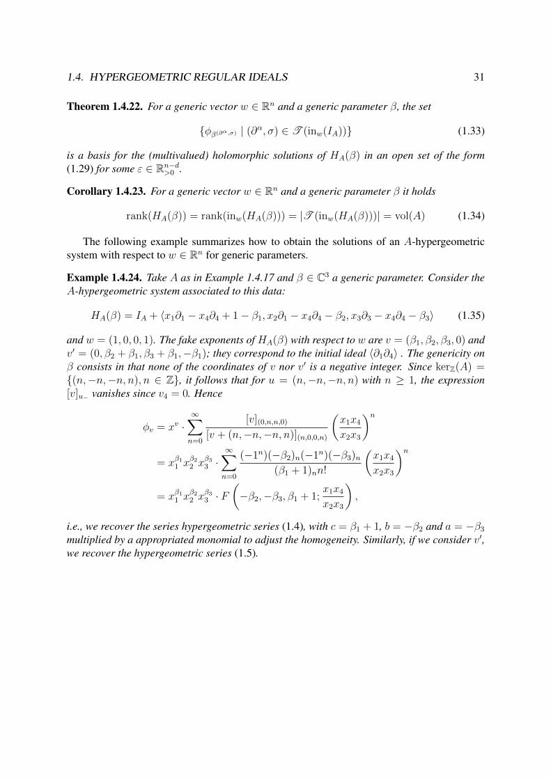
The following example summarizes how to obtain the solutions of an A-hypergeometricsystem with respect to w ∈ Rn for generic parameters.
Example 1.4.24. Take A as in Example 1.4.17 and β ∈ C3 a generic parameter. Consider theA-hypergeometric system associated to this data:
HA(β) = IA + 〈x1∂1 − x4∂4 + 1− β1, x2∂1 − x4∂4 − β2, x3∂3 − x4∂4 − β3〉 (1.35)
and w = (1, 0, 0, 1). The fake exponents of HA(β) with respect to w are v = (β1, β2, β3, 0) andv′ = (0, β2 + β1, β3 + β1,−β1); they correspond to the initial ideal 〈∂1∂4〉 . The genericity onβ consists in that none of the coordinates of v nor v′ is a negative integer. Since kerZ(A) ={(n,−n,−n, n), n ∈ Z}, it follows that for u = (n,−n,−n, n) with n ≥ 1, the expression[v]u− vanishes since v4 = 0. Hence
φv = xv ·∞∑n=0
[v](0,n,n,0)
[v + (n,−n,−n, n)](n,0,0,n)
(x1x4
x2x3
)n= xβ1
1 xβ2
2 xβ3
3 ·∞∑n=0
(−1n)(−β2)n(−1n)(−β3)n(β1 + 1)nn!
(x1x4
x2x3
)n= xβ1
1 xβ2
2 xβ3
3 · F(−β2,−β3, β1 + 1;
x1x4
x2x3
),
i.e., we recover the series hypergeometric series (1.4), with c = β1 + 1, b = −β2 and a = −β3
multiplied by a appropriated monomial to adjust the homogeneity. Similarly, if we consider v′,we recover the hypergeometric series (1.5).
32 CHAPTER 1. REGULAR A-HYPERGEOMETRIC SYSTEMS

Chapter 2
Tools from combinatorics
This chapter summarizes the tools from combinatorics that we need in the rest of the thesis.Coherent triangulations were treated in section 1.4.2 in the context of initial of toric ideals,but they are intimately related with the topics seen here. The Secondary Fan is the object thatdescribes all coherent triangulations for a given configuration. Coherent mixed subdivisionwill be used to define algebraic Laurent solutions of particular A-hypergeometric systems inChapter 6.
2.1 Secondary Fan
We now present the object that parametrizes all coherent triangulations of the configuration Aand, consequently, it also describes the regions of convergence of A-hypergeometric canonicalseries. This object is called the secondary fan of A, and was introduced by Gelfand, Kapranovand Zelevinsky (see [GKZ94, Chapter 7]). We summarize the construction of the secondaryfan and give some examples related with the ones previously given.
To construct the secondary fan of A, we need the following notion
Definition 2.1.1. A Gale dual for A is a matrix B ∈ Zn×(n−d) whose columns form a Z-basisfor kerZ(A).
Denote by b1, . . . , bn the rows of B, a Gale dual for A, and let ∆ be a coherent triangulationof A. For each maximal simplex σ ∈ ∆, we define a cone
Kσ =
{∑i/∈σ
λibi
∣∣∣∣ λi ≥ 0
}.
The set {bi | i /∈ σ} is linearly independent [GKZ94, Lemma 7.1.16], and therefore Kσ isfull-dimensional.
Define K∆ = ∩σ∈∆Kσ. Then w ∈ Rn is such that ∆w = ∆ if and only if w · B belongs tothe interior of K∆. The cones K∆ for all coherent triangulations ∆ of A are the maximal conesin a polyhedral fan, called the secondary fan of A (see also [GKZ94, Theorem 7.1.17]). It is inthis sense in which we say that the secondary fan parametrizes the coherent triangulations ofA.
33

34 CHAPTER 2. TOOLS FROM COMBINATORICS
Example 2.1.2. Consider A as in Example 1.1.4. We describe its coherent triangulations inExample 1.4.18. A Gale dual for the configuration A is given by
B =
1−2
1
.
Consider the coherent triangulation ∆1 = {{0, 1}, {1, 2}}. The one-dimensional cone K∆1
is the intersection of the cones K{0,1} and K{1,2} both equal to {λ ∈ R≥0} = R≥0, thatis K∆1 = R≥0. The vectors w ∈ R3 that induce this triangulation are the ones such thatw1 − 2w2 + w3 > 0.
On the other hand, the triangulation ∆2 = {{0, 2}} corresponds to the cone K∆2 =K{0,2} = {−2 · λ ∈ R≥0} = R≤0. The vectors w ∈ R3 that induce this triangulation arethe ones such that w1 − 2w2 + w3 < 0.
Next we consider an example where the secondary fan is two-dimensional.
Example 2.1.3. Let
A =
1 1 1 0 0 00 0 0 1 1 11 0 1 1 2 30 4 1 1 1 0
, B =
−1 2
0 11 −31 0−2 −1
1 1
.
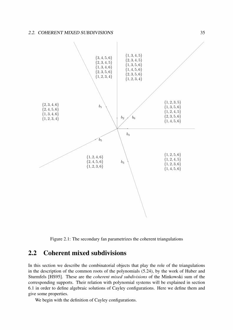
Being the configuration A a subset of R4 we cannot present the triangulations graphically. Toobtain the secondary fan, we simply draw the vectors bi, i = 1, . . . , 6 in a plane and considerthe positive cones generated pairwise by the row vectors bi. These are the intersections of thecones Kσ as σ runs over a coherent triangulation. Then the coherent triangulations of conv(A)are:
∆1 ={{1, 2, 3, 5}, {1, 3, 5, 6}, {1, 2, 4, 5}, {2, 3, 5, 6}, {1, 4, 5, 6}}∆2 ={{1, 3, 4, 5}, {2, 3, 4, 5}, {1, 3, 5, 6}, {1, 4, 5, 6}, {2, 3, 5, 6}, {1, 2, 3, 4}}∆3 ={{3, 4, 5, 6}, {2, 3, 4, 5}, {1, 3, 4, 6}, {2, 3, 5, 6}, {1, 2, 3, 4}}∆4 ={{2, 3, 4, 6}, {2, 4, 5, 6}, {1, 3, 4, 6}, {1, 2, 3, 4}}∆5 ={{1, 2, 4, 6}, {2, 4, 5, 6}, {1, 2, 3, 6}}∆6 ={{1, 2, 5, 6}, {1, 2, 4, 5}, {1, 2, 3, 6}, {1, 4, 5, 6}}
For instance, the triangulation ∆1 is associated to any vector w ∈ R6 such that the planar vec-tor bw =
∑6i=1wibi lies in the positive cone R>0b4 + R>0b6. This implies that the complemen-
tary indices {1, 2, 3, 5} form a maximal cell of ∆. Indeed, maximal cells correspond preciselyto the complementary indices of those pairs of vectors bi, bj such that bw ∈ R>0bi + R>0bj .
In Figure 2.1 we depict the secondary fan and indicate, in the interior of each cone, thecorresponding coherent triangulation.
2.2. COHERENT MIXED SUBDIVISIONS 35
b1
b2
b3
b4
b5
b6
{1, 2, 3, 5}{1, 3, 5, 6}{1, 2, 4, 5}{2, 3, 5, 6}{1, 4, 5, 6}
{1, 3, 4, 5}{2, 3, 4, 5}{1, 3, 5, 6}{1, 4, 5, 6}{2, 3, 5, 6}{1, 2, 3, 4}
{3, 4, 5, 6}{2, 3, 4, 5}{1, 3, 4, 6}{2, 3, 5, 6}{1, 2, 3, 4}
{2, 3, 4, 6}{2, 4, 5, 6}{1, 3, 4, 6}{1, 2, 3, 4}
{1, 2, 4, 6}{2, 4, 5, 6}{1, 2, 3, 6}
{1, 2, 5, 6}{1, 2, 4, 5}{1, 2, 3, 6}{1, 4, 5, 6}
Figure 2.1: The secondary fan parametrizes the coherent triangulations
2.2 Coherent mixed subdivisions
In this section we describe the combinatorial objects that play the role of the triangulationsin the description of the common roots of the polynomials (5.24), by the work of Huber andSturmfels [HS95]. These are the coherent mixed subdivisions of the Minkowski sum of thecorresponding supports. Their relation with polynomial systems will be explained in section6.1 in order to define algebraic solutions of Cayley configurations. Here we define them andgive some properties.
We begin with the definition of Cayley configurations.
36 CHAPTER 2. TOOLS FROM COMBINATORICS
Definition 2.2.1. Let A1, . . . , Ak ⊂ Zk be k lattice configurations in k-th dimensional space.Set n = |A1|+· · ·+|Ak| and d = 2k. We call Cayley configuration associated withA1, . . . , Ak,denoted by A = Cayley(A1, . . . , Ak), the configuration in Zd defined by
A = {e1}× A1 ∪ · · · ∪ {ek}×Ak. (2.1)
Our goal in Chapter 6 will be to describe the Laurent algebraic solutions for the A-hy-pergeometric systems associated to Cayley configurations (see Definition 2.2.1) (and integerhomogeneities). Based on Example 5.3.4, we will show that the common roots of the polyno-mials (5.24) play a special role in the description of such solutions.
In the univariate case, there is an intimate relation between the combinatorics of the con-figuration A and the regions where the roots ρ1(x), . . . , ρd(x) define holomorphic functions.Examples 5.1.6 and 1.4.18 show this relation: for w ∈ R3 such that the coherent triangulationof the configuration A is {{0, 1}, {1, 2}}, the roots can be written as Laurent series (see (5.8))converging in the open set ∣∣∣∣x0x2
x21
∣∣∣∣ << 1.
On the other hand, for w ∈ R3 such that the coherent triangulation of the configuration A is{{0, 2}}, there are no Laurent series in the direction of w, but the roots are still solutions ofHA(β) in the open set ∣∣∣∣ x2
1
x0x2
∣∣∣∣ << 1
and therefore, they can be written as Puiseaux series there with exponents in 12· Z. The roots
of any degree univariate polynomial behave in a similar way.Although the definitions can be given for an arbitrary k ∈ N we assume k = 2 for simplicity
of the exposition.Suppose that A1 = {α1, . . . , αr} and A2 = {β1, . . . , βs} are planar lattice configurations.
Set n = r + s.
Definition 2.2.2. Given w ∈ Rn a generic weight we denote by ∆w the corresponding coherenttriangulation of A = Cayley(A1, A2). The corresponding mixed coherent subdivision Πw ofA1 + A2 is defined as follows. The top dimensional cells of Πw are in bijection with the topdimensional cells in ∆w. Given any top dimensional cell τ in ∆w, must contain an index ineach of A1, A2. Note that dim(τ) = 3 and so |τ | = 4. The vertices of the corresponding cellστ in Πw are the points αi + βj , for each pair i, r + j ∈ τ with 1 ≤ i ≤ r and 1 ≤ j ≤ s.
We indicate the cell στ in Πw by the cell τ ⊂ {1, . . . , n} of ∆w. We say that στ is mixed if|τ ∩ Ai| = 2, i = 1, 2, and unmixed otherwise.
Remark 2.2.3. Mixed subdivisions can be defined in terms of liftings of A1 +A2 as in [HS95];see [DRS10, Section 9.2] for the equivalence of both definitions.
Let w ∈ Rn generic. The following proposition is an easy consequence of the definiton ofcoherent mixed subdivision, and Theorem 1.4.16.
Proposition 2.2.4. Let w be a generic weight in Rn and call Πw the associated mixed coherentsubdivision of A1 + A2. Let σ ∈ Πw. The following statements are equivalent:
2.2. COHERENT MIXED SUBDIVISIONS 37
1. σ is a cell in Πw.
2. For all σ′ ⊆ σ call Γσ′ = {u ∈ kerA : ui < 0 ⇔ i ∈ σ′}. Then 〈w, u〉 > 0 for allu ∈ Γσ′ , u 6= 0.
3. No initial monomial in inw(IA) has support (contained) in σ.
Remark 2.2.5. Note that Γσ′ could be empty. For instance, if αi + βj is a vertex of A1 + A2
and σ′ = {i, r + j}, then Γσ′ = ∅. This implies that all vertices automatically satisfy 2. andthen, they belong to any Πw, which is obvious.
Before giving examples of coherent mixed subdivisions, we prove a technical lemma thatwill be used in section 6.2.
Lemma 2.2.6. Let w ∈ Rn generic and σ ⊂ Πw a mixed cell. Let I ( σ and rI 6= ∅. Thenthere exists w′ ∈ Rn such that σ ⊂ Πw′ and I * Πw′ .
Proof. Suppose I = {i1, . . . , ik}. Given that rI 6= ∅, there exists a binomial of the form
bI = ∂u1i1. . . ∂ukik − ∂
v(I) ∈ IA,
where ui ∈ N, i = 1, . . . , k and v(I)j = 0 for all j ∈ I . As I ( σ there exists 1 ≤ j ≤ k suchthat ij ∈ I−σ. Set w′ = w+λeij with λ sufficiently large so that inw′(bI) = ∂u1
i1. . . ∂ukik . Then
I * Πw′ .To see that σ ⊂ Πw′ , note that by hypothesis and Proposition 2.2.4, no initial monomial in
inw(IA) has support contained in σ. Given that ij /∈ σ, it is clear that no initial monomial withrespect to w′ will have support contained in σ.
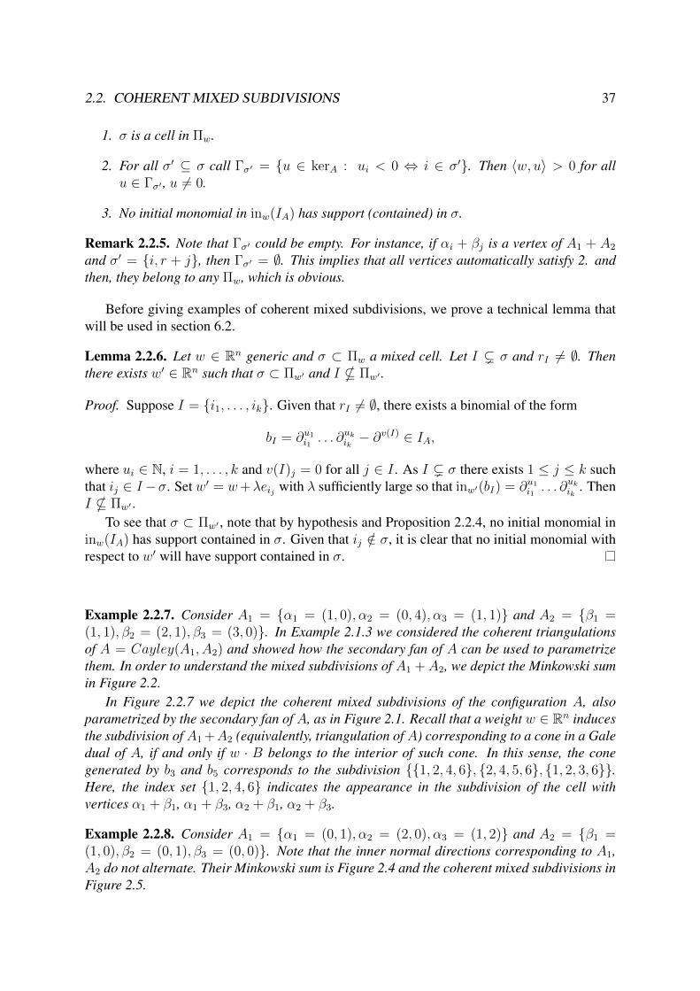
Example 2.2.7. Consider A1 = {α1 = (1, 0), α2 = (0, 4), α3 = (1, 1)} and A2 = {β1 =(1, 1), β2 = (2, 1), β3 = (3, 0)}. In Example 2.1.3 we considered the coherent triangulationsof A = Cayley(A1, A2) and showed how the secondary fan of A can be used to parametrizethem. In order to understand the mixed subdivisions of A1 +A2, we depict the Minkowski sumin Figure 2.2.
In Figure 2.2.7 we depict the coherent mixed subdivisions of the configuration A, alsoparametrized by the secondary fan of A, as in Figure 2.1. Recall that a weight w ∈ Rn inducesthe subdivision of A1 +A2 (equivalently, triangulation of A) corresponding to a cone in a Galedual of A, if and only if w · B belongs to the interior of such cone. In this sense, the conegenerated by b3 and b5 corresponds to the subdivision {{1, 2, 4, 6}, {2, 4, 5, 6}, {1, 2, 3, 6}}.Here, the index set {1, 2, 4, 6} indicates the appearance in the subdivision of the cell withvertices α1 + β1, α1 + β3, α2 + β1, α2 + β3.
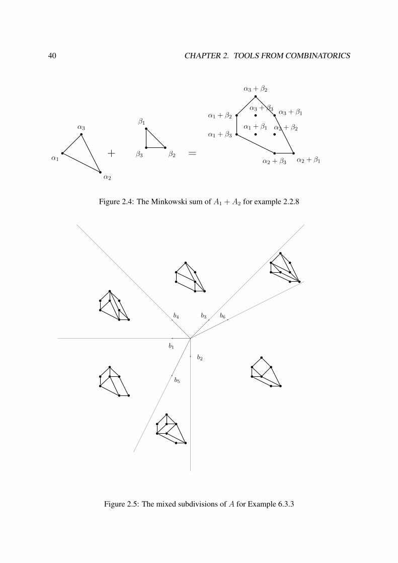
Example 2.2.8. Consider A1 = {α1 = (0, 1), α2 = (2, 0), α3 = (1, 2)} and A2 = {β1 =(1, 0), β2 = (0, 1), β3 = (0, 0)}. Note that the inner normal directions corresponding to A1,A2 do not alternate. Their Minkowski sum is Figure 2.4 and the coherent mixed subdivisions inFigure 2.5.

38 CHAPTER 2. TOOLS FROM COMBINATORICS
b
α1
b
α2
bα3
+
b
β1b
β2
b
β3
=
b
α1 + β1b
α1 + β2
b α1 + β3
b
α2 + β1b
α2 + β2
bα2 + β3
b
α3 + β1b
α3 + β2
b α3 + β3
Figure 2.2: The Minkowski sum of A1 + A2 for Example 2.2.7
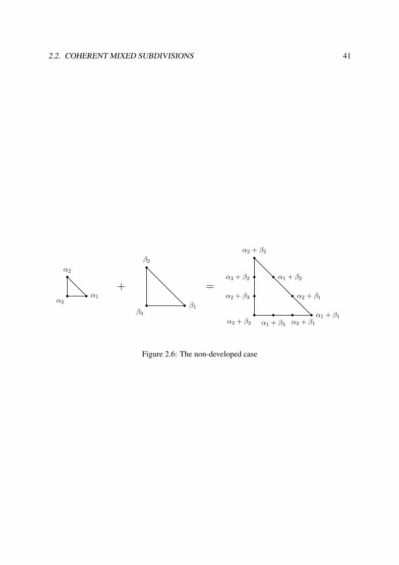
Example 2.2.9. ForA1 = {α1 = (1, 0), α2 = (0, 1), α3 = (0, 0)} andA2 = {β1 = (2, 0), β2 =(0, 2), β3 = (0, 0)} we depict the Minkowski sum in Figure 2.6. In this case the convex hullsof A1 and A2 have the same inner normals, and so this is an example of two non-developedpolytopes (cf. Section 5.4.1). Notice that the Minkowski sum does not have any interior pointsof the form αi + βj . Also notice that the six possible coherent mixed subdivisions, depicted inFigure 2.7, consist of one mixed cell and two unmixed cells.
The following two examples concern the case |A1| = 2 and |A2| = 4, to be discussed inChapter 6.
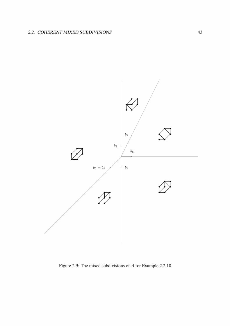
Example 2.2.10. Let A1 = {α1 = (0, 0), α2 = (1, 1)} and A2 = {β1 = (0, 0), β2 =(1, 0), β3 = (0, 1), β4 = (1, 1)}. The Minkowski sum of the segment and the square is de-picted in Figure 2.8. In this case the two interior point coincide, that is α1 +β4 = α2 +β1. Thecoherent mixed subdivisions are depicted in Figure 2.9.
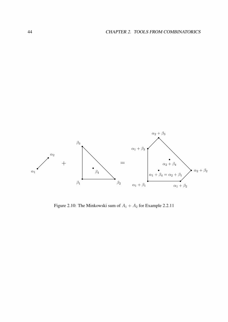
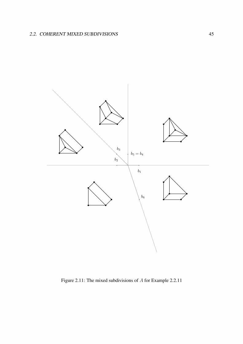
Example 2.2.11. Let A1 = {α1 = (0, 0), α2 = (1, 1)} and A2 = {β1 = (0, 0), β2 =(3, 0), β3 = (0, 3), β4 = (1, 1)}, which has an interior point. Their Minkowski sum is de-picted in Figure 2.10. In this case, there are two interior points: (1, 1) = α1 + β4 = α2 + β1
and (2, 2) = α2 + β4. The coherent mixed subdivisions are depicted in Figure 2.11.

2.2. COHERENT MIXED SUBDIVISIONS 39
b1
b2
b
b
b b
b
b
b3
b4
b5
b6b b
b
b b
b
b
b
b b
b
b b
b
b b
b
b
b
b b
b
b b
b
b
b
b b
b
b
b
b b
b
b b
b
b
Figure 2.3: The mixed subdivisions of A for Example 2.2.7.
40 CHAPTER 2. TOOLS FROM COMBINATORICS
b
α1
b
α2
b
α3
+
b
β1
b
β2
b
β3 =
bα1 + β3
bα1 + β2
b
α3 + β2
b α3 + β1
b
α2 + β1
b
α2 + β3
b
α2 + β2b
α1 + β1
b
α3 + β3
Figure 2.4: The Minkowski sum of A1 + A2 for example 2.2.8
b1
b2
b3b4
b5
b6
b
b
b
b
bb
b
b
b
b
b
bb
bb
b
b
b
b
bb
b
b
b
b
b
bb
b
b
b
b
b
b
bb
b
b
b
b
b
bb
b
b
Figure 2.5: The mixed subdivisions of A for Example 6.3.3
2.2. COHERENT MIXED SUBDIVISIONS 41
b α1
b
α2
b
α3
+
b β1
b
β2
b
β3
=
b α1 + β1
b α1 + β2
b
α2 + β2
bα2 + β3
b
α3 + β3
b
α3 + β1
b α2 + β1
b
α1 + β3
bα3 + β2
Figure 2.6: The non-developed case

42 CHAPTER 2. TOOLS FROM COMBINATORICS
b4
b2
b3 b1
b5
b6b
b
b
b
b b
b
b
b
b
b
b
b
b b
b
b
b
b
b
b
b
b b
b
b
b
b
b
b
b
b b
b
b
b
b
b
b
b
b b
b
b
b b
b
b
b
b b
b
b
b
Figure 2.7: The mixed subdivisions of A for Example 2.2.9
b
α1
bα2
+b
β1
b
β2
b
β3b
β4
=
b
α1 + β1
b
α1 + β2
bα1 + β3 b
α1 + β4 = α2 + β1
b
α2 + β2
b
α2 + β3b
α2 + β4
Figure 2.8: The Minkowski sum of A1 + A2 for Example 2.2.10
2.2. COHERENT MIXED SUBDIVISIONS 43
b1
b2
b6
b5 = b4
b3b b
b b
b b
b b
b b b
b b
b b
b b b
b b
b b
b b b
b b b b
b b b
b b
Figure 2.9: The mixed subdivisions of A for Example 2.2.10
44 CHAPTER 2. TOOLS FROM COMBINATORICS
b
α1
bα2
+
b
β1
b
β2
b
β3
b
β4
=
b
α1 + β1
b
α1 + β2
bα1 + β3
b
α1 + β4 = α2 + β1
b α2 + β2
b
α2 + β3
b
α2 + β4
Figure 2.10: The Minkowski sum of A1 + A2 for Example 2.2.11
2.2. COHERENT MIXED SUBDIVISIONS 45
b2
b5 = b4
b1
b6
b3
b b
b
b b
b
b
b b
b
b b
b
b
b b
b
b b
b
b b
b
b
b
b b
b
b b
b
Figure 2.11: The mixed subdivisions of A for Example 2.2.11

46 CHAPTER 2. TOOLS FROM COMBINATORICS
Chapter 3
Formal Nilsson solutions of irregularA-hypergeometric systems
One of the main properties of regular systems, based on important results by Malgrange in theunidimensional case and Mebkhout in the general case, resides in that one does not need toprove that a formal solution converges; as we saw in Chapter 1, this happens “automatically”.We recalled in Theorem 1.4.2 that if the row span of A contains the vector (1, . . . , 1), then thesystem HA(β) is regular. If this is not the case, Schulze and Walther [SW08] proved that thesystem is not regular. In this chapter we will not assume that the row span of A contains thevector (1, . . . , 1) and we will reprove in Theorem 3.5.6 their result. Our proof will deal withformal solutions of general A-hypergeometric systems, so that, in Section 3.1 we introduce thenotion of formal Nilsson solutions, which is an extension of the regular case. To that end, weintroduce a suitable notion of weight vector w ∈ Rn
≥0. The space of formal Nilsson solutionsis then established and we prove its relation with an associated regular system in Section 3.2,using the operation of homogenization. When the parameters are generic, the action of thehomogenization becomes more clear and we will be able, in Section 3.3, to calculate in com-binatorial terms the dimension of the space of formal Nilsson solutions as well as to give anexplicit basis of it. For general parameters, we study homogenization of logarithm-free formalNilsson solutions in Section 3.4. Finally, in Section 3.5 we use the developed tools to give thementioned alternative proof of the result of Schulze and Walther.
3.1 Initial ideals and formal Nilsson series
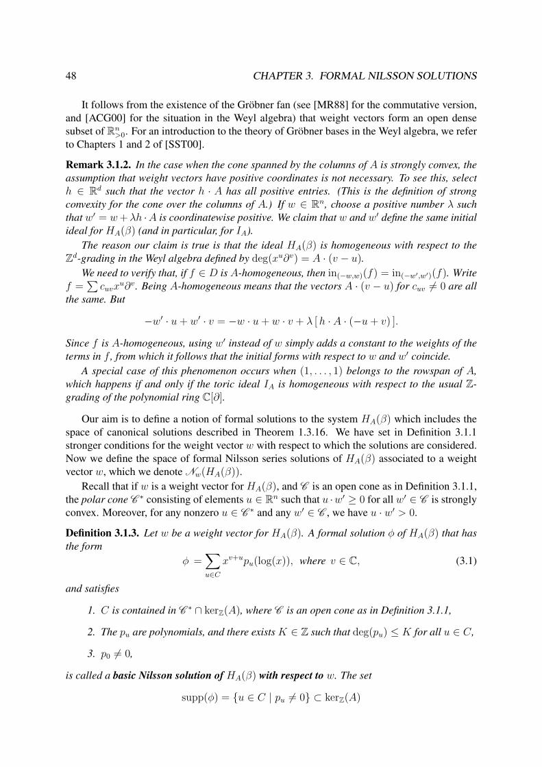
The following definition characterizes the weight vectors we consider in this and in the follow-ing chapter. Recall that a cone is strongly convex if it contains no lines.
Definition 3.1.1. A vector w ∈ Rn>0 is a weight vector for HA(β) if there exists a strongly
convex open rational polyhedral cone C , C \ {0} ⊂ Rn>0, with w ∈ C , such that, for all
w′ ∈ C , we have
inw(IA) = inw′(IA) and in(−w,w)(HA(β)) = in(−w′,w′)(HA(β)).
In particular, inw(IA) is a monomial ideal.
47
48 CHAPTER 3. FORMAL NILSSON SOLUTIONS
It follows from the existence of the Grobner fan (see [MR88] for the commutative version,and [ACG00] for the situation in the Weyl algebra) that weight vectors form an open densesubset of Rn
>0. For an introduction to the theory of Grobner bases in the Weyl algebra, we referto Chapters 1 and 2 of [SST00].
Remark 3.1.2. In the case when the cone spanned by the columns of A is strongly convex, theassumption that weight vectors have positive coordinates is not necessary. To see this, selecth ∈ Rd such that the vector h · A has all positive entries. (This is the definition of strongconvexity for the cone over the columns of A.) If w ∈ Rn, choose a positive number λ suchthat w′ = w+λh ·A is coordinatewise positive. We claim that w and w′ define the same initialideal for HA(β) (and in particular, for IA).
The reason our claim is true is that the ideal HA(β) is homogeneous with respect to theZd-grading in the Weyl algebra defined by deg(xu∂v) = A · (v − u).
We need to verify that, if f ∈ D is A-homogeneous, then in(−w,w)(f) = in(−w′,w′)(f). Writef =
∑cuvx
u∂v. Being A-homogeneous means that the vectors A · (v − u) for cuv 6= 0 are allthe same. But
−w′ · u+ w′ · v = −w · u+ w · v + λ [h · A · (−u+ v) ].
Since f is A-homogeneous, using w′ instead of w simply adds a constant to the weights of theterms in f , from which it follows that the initial forms with respect to w and w′ coincide.
A special case of this phenomenon occurs when (1, . . . , 1) belongs to the rowspan of A,which happens if and only if the toric ideal IA is homogeneous with respect to the usual Z-grading of the polynomial ring C[∂].
Our aim is to define a notion of formal solutions to the system HA(β) which includes thespace of canonical solutions described in Theorem 1.3.16. We have set in Definition 3.1.1stronger conditions for the weight vector w with respect to which the solutions are considered.Now we define the space of formal Nilsson series solutions of HA(β) associated to a weightvector w, which we denote Nw(HA(β)).
Recall that if w is a weight vector for HA(β), and C is an open cone as in Definition 3.1.1,the polar cone C ∗ consisting of elements u ∈ Rn such that u ·w′ ≥ 0 for all w′ ∈ C is stronglyconvex. Moreover, for any nonzero u ∈ C ∗ and any w′ ∈ C , we have u · w′ > 0.
Definition 3.1.3. Let w be a weight vector for HA(β). A formal solution φ of HA(β) that hasthe form
φ =∑u∈C
xv+upu(log(x)), where v ∈ C, (3.1)
and satisfies
1. C is contained in C ∗ ∩ kerZ(A), where C is an open cone as in Definition 3.1.1,
2. The pu are polynomials, and there exists K ∈ Z such that deg(pu) ≤ K for all u ∈ C,
3. p0 6= 0,
is called a basic Nilsson solution of HA(β) with respect to w. The set
supp(φ) = {u ∈ C | pu 6= 0} ⊂ kerZ(A)
3.1. INITIAL IDEALS AND FORMAL NILSSON SERIES 49
is called the support of φ.The C-span of the basic Nilsson solutions of HA(β) with respect to w is called the space of
formal Nilsson series solutions of HA(β) with respect to w and is denoted by Nw(HA(β)).
Remark 3.1.4. Given a weight vector w, we may replace the first requirement in Defini-tion 3.1.3 by either of the following equivalent conditions:
i) C ⊂ kerZ(A) and there exists an open neighborhood U of w such that, for all w′ ∈ U andall u ∈ C r {0}, we have w′ · u > 0.
ii) There exist R-linearly independent γ1, . . . , γn ∈ Qn with w · γi > 0 for all i = 1, . . . , n,such that C ⊂
(R≥0γ1 + · · ·+ R≥0γn
)∩ kerZ(A).
Remark 3.1.5. If w is a weight vector for HA(β) and C is a strongly convex open cone asin Definition 3.1.1, then for any w′ ∈ C , the exponents of HA(β) with respect to w and w′
coincide. Moreover, the basic Nilsson solutions of HA(β) with respect to w and w′ are thesame, and therefore Nw(HA(β)) = Nw′(HA(β)).
Lemma 3.1.6. If φ is a basic Nilsson solution of HA(β) with respect to w as in (3.1), then v isan exponent of HA(β) with respect to w.
Proof. Since w is a weight vector, w · u > 0 for all u ∈ C ∗. This implies that inw(φ) =xvp0(log(x)). Thus, xvp0(log(x)) is a solution of in(−w,w)(HA(β)) by Theorem 1.3.9. But thenxv is a solution of the initial ideal in(−w,w)(HA(β)) by [SST00, Theorems 2.3.3(2) and 2.3.11].
Compare the following definition with Definition 1.3.17.
Definition 3.1.7. Solutions of HA(β) of the form (3.1) that satisfy the first two conditions inDefinition 3.1.3 are called series solution of HA(β) in the direction of w. The C-span of allsuch series is called the space of series solutions of HA(β) in the direction of w.
Most of the considerations about the ring Nw can be made also on Nw(HA(β)). We canconsider the term order (1.18) and manipulate the series in the same way. This is a version ofLemma 1.3.10 that clearly holds for Nw(HA(β)):
Lemma 3.1.8. Let φ1, . . . , φk ∈ Nw(HA(β)).
1. If the initial series inw(φ1), . . . , inw(φk) are C-linearly independent, then φ1, . . . , φk areC-linearly independent.
2. If φ1, . . . , φk are C-linearly independent, there exists a k×k complex matrix (λij) such thatthe initial series of ψi =
∑kj=1 λijφj for i = 1, . . . , k are C-linearly independent.
We can compare the dimension of the space of formal Nilsson solutions of HA(β) withrespect to w with the holonomic rank of the associated initial ideal.
Proposition 3.1.9. Let w be a weight vector for HA(β). Then
dimC(Nw(HA(β))) ≤ rank(in(−w,w)(HA(β))). (3.2)
50 CHAPTER 3. FORMAL NILSSON SOLUTIONS
Proof. Choose ψ1, . . . , ψk linearly independent elements of Nw(HA(β)). The second part ofLemma 3.1.8 allows us to assume that the series inw(ψ1), . . . , inw(ψk) are linearly indepen-dent solutions of the initial system in(−w,w)(HA(β)). These initial series have a non emptycommon open domain of convergence since they have a finite number of terms. ThereforedimC(Nw(HA(β))) cannot exceed the holonomic rank of in(−w,w)(HA(β)).
We show in Corollary 3.3.12 that this inequality is, in fact, an equality for generic β. IfIA is a homogeneous ideal, dimC Nw(HA(β)), rank(in(−w,w)(HA(β))), and rank(HA(β)) arethe same (see Proposition 3.1.10 below). However, if IA is not homogeneous, we will prove inCorollary 3.3.13 that rank(in(−w,w)(HA(β))) does not always equal rank(HA(β)).
Finally, we show that this notion of formal solution coincide with the known space of solu-tions for the regular case.
Proposition 3.1.10. If the row span of A contains the vector (1, . . . , 1) and w ∈ Rn is aweight vector then the space generated by the canonical series coincides with Nw(HA(β)). Inparticular
dimC(Nw(HA(β))) = rank(HA(β)). (3.3)
Proof. By Theorem 1.4.2 we know that HA(β) is regular holonomic. Then, by Proposition3.1.9 and Theorem 1.3.11 we have that
dimC(Nw(HA(β))) ≤ rank(HA(β)). (3.4)
On the other hand, any canonical solution ofHA(β) is, by definition, a basic solution ofHA(β).This means that the space spanned by the canonical series solutions ofHA(β), whose dimensionis rank(HA(β)), is less or equal that dimC(Nw(HA(β))). This concludes the proof.
3.2 Homogenization of formal Nilsson solutions of HA(β)
The goal of this section is to obtain the solutions of the system HA(β) by solving a relatedhypergeometric system that is regular holonomic. For generic parameters, this idea was used inother works, such as [OT09]; here, we require no genericity hypotheses on β. The key conceptis that of homogenization.
Notation 3.2.1. Throughout this and the following chapter, the letter ρ is used to indicate thehomogenization of various objects: polynomials, ideals, and later on, Nilsson series.
If f ∈ C[∂1, . . . , ∂n] is a polynomial, we denote by ρ(f) ∈ C[∂0, ∂1, . . . , ∂n] its homoge-nization, that is,
f =∑u∈Nn
cu∂u =⇒ ρ(f) =
∑u∈Nn
cu∂deg(f)−|u|0 ∂u, |u| = u1 + · · ·+ un.
If I ⊆ C[∂1, . . . , ∂n] is an ideal, then
ρ(I) = 〈ρ(f) | f ∈ I〉 ⊆ C[∂0, ∂1, . . . , ∂n].
3.2. HOMOGENIZATION OF FORMAL NILSSON SOLUTIONS OF HA(β) 51
If A = [aij] is a d × n integer matrix, then ρ(A) ∈ Z(d+1)×(n+1) is obtained by attachinga column of zeros to the left of A, and then attaching a row of ones to the resulting matrix,namely
ρ(A) =
1 1 . . . 10 a11 . . . a1n...
......
0 ad1 . . . adn
.
Note thatρ(IA) = Iρ(A).
Let w be a weight vector for HA(β) and fix β0 ∈ C. Let Hρ(A)(β0, β) be the (regularholonomic) hypergeometric system associated to the matrix ρ(A) from Notation 3.2.1 and thevector (β0, β) ∈ Cn+1. Since the set of weight vectors for Hρ(A)(β0, β) is an open dense subsetof Rn+1
>0 , there exists α = (α0, . . . , αn) ∈ Rn+1 and ε0 > 0 such that (0, w) + εα is a weightvector for Hρ(A)(β0, β) for all 0 < ε < ε0. But then (0, w) + εα − εα0(1, . . . , 1) is alsoa weight vector for Hρ(A)(β0, β), because Iρ(A) is homogeneous (see Remark 3.1.2). If ε issufficiently small, then w′ = w + ε((α1, . . . , αn) − α0(1, . . . , 1)) belongs to the open cone Cfrom Definition 3.1.1. This means that we can use w′ instead of w as weight vector for HA(β),with the same open cone, initial ideals, and basic Nilsson solutions as w, and guarantee that(0, w′) is a weight vector for Hρ(A)(β0, β).
This justifies assuming, as we do from now on, that any time we choose a weight vector wfor HA(β), the vector (0, w) is a weight vector for Hρ(A)(β0, β).
We have chosen a weight vector w, and we wish to use the auxiliary system Hρ(A)(β0, β)to study the solutions of HA(β). The matrix ρ(A) is fixed, but we have freedom in the choiceof the parameter β0 ∈ C, and it is convenient to assume that β0 is generic. The correct notionof genericity for β0 can be found in Definition 3.2.4. Under that hypothesis, our objective is toconstruct an injective linear map
ρ : Nw(HA(β)) −→ N(0,w)(Hρ(A)(β0, β)), (3.5)
whose image is described in Theorem 3.2.12. For some weight vectors, ρ is guaranteed to besurjective (Proposition 3.5.1). However, if the cone over the columns of A is strongly convexand IA is not homogeneous, there always exist weights for which surjectivity fails (Proposi-tion 3.5.4).
Let φ =∑
u∈C xv+upu(log(x)) be a basic Nilsson solution of HA(β) with respect to w as
in (3.1). Since φ is annihilated by the Euler operators E1 − β1, . . . , Ed − βd, the polynomialspu appearing in φ belong to the symmetric algebra of the lattice kerZ(A) by [Sai02, Proposition5.2]. More explicitly, let {γ1, . . . , γn−d} ⊂ Zn be a Z-basis of kerZ(A). Then we can write
pu(t1, . . . , tn) =∑
α∈Nn−dcα
n−d∏j=1
(γj · (t1, . . . , tn))αj .
For such a pu, define
pu(t0, t1, . . . , tn) =∑
α∈Nn−dcα
n−d∏j=1
((−|γj|) t0 + γj · (t1, . . . , tn))αj , (3.6)
52 CHAPTER 3. FORMAL NILSSON SOLUTIONS
where, for any vector v = (v1, . . . , vn) ∈ Cn, |v| =∑n
i=1 vi. Note that pu specializes to puwhen x0 = 1, or equivalently, when log(x0) = 0.
The formal definition of the homogenization of the series φ =∑
u∈C xv+upu(log(x)) is
ρ(φ) =∑u∈C
∂|u|0 x
β0−|v|0 xv+upu(log(x0), . . . , log(xn)). (3.7)
If |u| ≥ 0 for all u ∈ C, the above formula makes sense, and it easily checked that ρ(φ) isa basic Nilsson solution of Hρ(A)(β0, β) with respect to (0, w). The bulk of the work in thissection concerns the definition and properties of the operator ∂k0 when k ∈ Z<0.
We point out that there is one case when the elements of the supports of all basic Nilssonsolutions of HA(β) with respect to w are guaranteed to have non negative coordinate sum,namely when the weight vector w is close to (1, . . . , 1). We make this notion precise in thefollowing definition.
Definition 3.2.2. Let w be weight vector for HA(β). We say that w is a perturbation of w0 ∈Rn>0 if there exists an open cone C as in Definition 3.1.1 with w ∈ C , such that w0 lies in the
closure of C .
Suppose that φ = xv∑
u∈C xupu(log(x)) is a basic Nilsson solution of HA(β) with respect
to a weight vectorw which is a perturbation of (1, . . . , 1). Since u ∈ C implies u ∈ C ∗ = (C )∗,we have u · w ≥ 0 for all u ∈ C. But then, as C ⊂ Zn and w is a perturbation of (1, . . . , 1), itfollows that |u| = u · (1, . . . , 1) ≥ 0 for all u ∈ C. Thus, the operator ∂|u|0 is defined, and sois (3.7).
As we mentioned before, in order to work with other weight vectors, we need to define theoperator ∂k0 when k is negative.
Recall that in(0,w)(Iρ(A)) is a monomial ideal, as (0, w) is a weight vector for Hρ(A)(β0, β).A standard pair of in(0,w)(Iρ(A)) is said to pass through zero if 0 ∈ σ.
Definition 3.2.3. We say that a basic Nilsson solution of HA(β) as in (3.1) is associated to thestandard pair (∂α, σ) if v is the (fake) exponent corresponding to this standard pair.
The following definition gives the correct notion of genericity for β0 ∈ C so that we canstudy the solutions of HA(β) using those of Hρ(A)(β0, β).
Definition 3.2.4. Let w be a weight vector for HA(β). We say that β0 is a homogenizing valuefor A, β, and w if β0 /∈ Z and for any fake exponent v of HA(β) with respect to w, we havev0 = β0 −
∑nj=1 vj /∈ Z.
Given a weight vector w for HA(β), we fix a homogenizing value β0 for A, β, and w. Letφ as in (3.1) be a basic Nilsson solution of HA(β) with respect to w. We want to construct abasic Nilsson solution ρ(φ) of Hρ(A)(β0, β) with respect to (0, w).
The following lemma tells us how to differentiate logarithmic terms.
Lemma 3.2.5. [Sai02, Lemma 5.3] Let h be a polynomial in r variables, ν ∈ Nr and s ∈ Cr.Then
∂νxsh(log(x)) = xs−ν( ∑
0≤ν′≤νλν′
[∂ν−ν
′h
](log(x))
),

3.2. HOMOGENIZATION OF FORMAL NILSSON SOLUTIONS OF HA(β) 53
where the sum is over nonnegative integer vectors ν ′ that are coordinatewise smaller than ν,and the λν′ are complex numbers.
Lemma 3.2.6. Let p be a polynomial in n + 1 variables, and s ∈ Cn. If s0 ∈ C and s0 6= −1,there exists a unique polynomial q with deg(q) = deg(p) such that
∂0
[xs0+1
0 xsq(log(x0), . . . , log(xn))]
= xs00 xsp(log(x0), . . . , log(xn)). (3.8)
Proof. Writing
p(log(x)) =k∑i=0
pi(log(x1), . . . , log(xn)) log(x0)i
and
q(log(x)) =k∑i=0
qi(log(x1), . . . , log(xn)) log(x0)i,
we can equate coefficients in (3.8) to obtain
pk = (s0 + 1)qk ; pi = (s0 + 1)qi + (i+ 1)qi+1 0 ≤ i ≤ k − 1.
Therefore
qi =k−i∑`=0
(−1)`∏`
j=1(i+ j)
(s0 + 1)`pi+` 0 ≤ ` ≤ k,
where the empty product is defined to be 1.
Definition 3.2.7. With the notation of Lemma 3.2.6, define
∂−10
[xs00 x
sp(log(x0), . . . , log(xn))]
= xs0+10 xsq(log(x0), . . . , log(xn)).
Note that if s0 6= −2, . . . ,−k, the construction of ∂−10 can be iterated (k− 1) times. We denote
by ∂−k0
[xs00 x
sp(log(x0), . . . , log(xn))]
the outcome of this procedure.
Lemma 3.2.8. Use the same notation and hypotheses as in Lemma 3.2.6, and assume further-more that xs00 x
sp(log(x)) is a solution of 〈E0 − β0, E − β〉. Then ∂−10 [xs00 x
sp(log(x))] is asolution of 〈E0− (β0 + 1), E− β〉. If s0 6= −2, . . . ,−k, then ∂−k0 [xs00 x
sp(log(x))] is a solutionof the system 〈E0 − (β0 + k), E − β〉.
Proof. If i > 0, ∂0(Ei − βi) = (Ei − βi)∂0, so that
∂0(Ei − βi)(∂−10 xs00 x
sp(log(x))) = (Ei − βi)∂0(∂−10 xs00 x
sp(log(x)))
= (Ei − βi)xs00 xsp(log(x))
= 0.
This means that (Ei − βi)(∂−10 xs00 x
sp(log(x))) is constant with respect to x0. On the otherhand, s0 + 1 6= 0 and (Ei− βi)(∂−1
0 xs00 xsp(log(x))) is a multiple of xs0+1. Thus, in order to be
constant with respect to x0, (Ei−βi)(∂−10 xs00 x
sp(log(x))) must vanish. For i = 0, the argumentis similar since ∂0(E0 − (β0 + 1)) = (E0 − β0)∂0. The last assertion follows by induction onk.
54 CHAPTER 3. FORMAL NILSSON SOLUTIONS
Lemma 3.2.9. Let ν ∈ Nn, k ∈ Z, and assume that s0 /∈ Z. Then
∂ν[∂k0[xs00 x
sp(log(x0), . . . , log(xn))]]
= ∂k0[∂ν[xs00 x
sp(log(x0), . . . , log(xn))]].
Proof. This is clear if k ≥ 0. For k < 0, the result follows by induction from the uniquenesspart of Lemma 3.2.6.
We are now ready to define the homogenization of a basic Nilsson solution of HA(β).
Definition 3.2.10. Let φ = xv∑
u∈C xupu(log(x)) be a basic Nilsson solution of HA(β) with
respect to a weight vector w, and let β0 ∈ C a homogenizing value for A, β and w, so thatv0 = β0 −
∑ni=1 vi is not an integer. Thus, we may define
ρ(φ) =∑u∈C
∂|u|0
[xv0
0 xv+upu(log(x0), log(x1), . . . , log(xn))
],
where pu is obtained from pu as in (3.6).
Proposition 3.2.11. Let w be a weight vector with respect to HA(β) (which, by assumptionimplies that (0, w) is a weight vector for Hρ(A)(β0, β), where β0 is our fixed homogenizingvalue for A, β and w). For any basic Nilsson solution φ = xv
∑xupu(log(x)) of HA(β)
with respect to w, the (formal) series ρ(φ) from Definition 3.2.10 is a basic Nilsson solution ofHρ(A)(β0, β) with respect to (0, w). We extend ρ linearly to obtain a map
ρ : Nw(HA(β))→ N(0,w)(Hρ(A)(β0, β)).
Proof. We first show that the series ρ(φ) has the shape required in Definition 3.1.3. Condi-tions 2 and 3 are clearly satisfied by the construction of the polynomials pu and Lemma 3.2.5.Thus, we need to verify that ρ(φ) satisfies condition (i) from Remark 3.1.4. The support of φ isin bijection with the support of ρ(φ) via u 7→ (−|u|, u), which sends kerZ(A) into kerZ(ρ(A)).We can assume that C is the intersection of kerZ(A) with the dual C ∗ of an open cone C suchthat its closure C is a strongly convex rational polyhedral cone of maximal dimension. Let{γ1, . . . , γm} be a Hilbert basis of C ∗ ∩ kerZ(A) = (C )∗ ∩ kerZ(A). Then w′ · γi > 0 for allw′ ∈ C and all i = 1, . . . ,m. Let δ > 0 such that, for all ε ∈ Rn+1
>0 whose Euclidean distanceto the origin is ||ε|| < δ, and all i = 1, . . . ,m, we have
[(0, w) + ε
]· (−|γi|, γi) > 0. It follows
that for any non zero u ∈ C and any w in the ball centered at (0, w) with radius δ, we havew · (−|u|, u) > 0, which proves our claim.
Now we prove that ρ(φ) is a formal solution of Hρ(A)(β0, β). Since pu belongs to thesymmetric algebra of kerZ(ρ(A)), and
ρ(A) · (v0, v + u) = (β0 − |v|+ |v|+ |u|, A · (v + u)) = (β0 + |u|, β),
the term xv00 x
v+upu(log(x0), log(x1), . . . , log(xn)) is a solution of the system of Euler operators〈E0−(β0+|u|), E1−β1, . . . , Ed−βd〉. By Lemma 3.2.8 with (s0, s) = (v0, v+u) and k = −|u|,each term of ρ(φ) is therefore a solution of 〈E − (β0 + |u| − |u|), E1 − β1, . . . , Ed − βd〉.
To verify that the elements of Iρ(A) annihilate ρ(φ), first note that Lemma 3.2.5 implies thatfor any µ ∈ kerZ(A)
∂µ+xv+upu(log(x)) = ∂µ−xv+u−µpu−µ(log(x)),
3.2. HOMOGENIZATION OF FORMAL NILSSON SOLUTIONS OF HA(β) 55
because φ is a solution of HA(β).We claim that
∂µ+xv00 x
v+upu(log(x)) = ∂µ−xv00 x
v+u−µpu−µ(log(x)).
To see this, use Lemma 3.2.5 and the fact that, if i > 0 and p is an element of the symmetricalgebra of kerZ(A), then ∂ip is also in the symmetric algebra of kerZ(A), and ∂ip = ∂ip.
Now, using Lemma 3.2.9 with (s0, s) = (v0, v + u) and k = |u|, and the fact that v0 =β0 − |v| /∈ Z, we obtain from
∂|u|0 ∂µ+xv0
0 xv+upu(log(x)) = ∂
|µ|0 ∂
|u|−|µ|0 ∂µ−xv0
0 xv+u−µpu−µ(log(x)),
that∂µ+
[∂|u|0 xv0
0 xv+upu(log(x))
]= ∂
|µ|0 ∂µ−
[∂|u|−|µ|0 xv0
0 xv+u−µpu−µ(log(x))
].
Assuming |µ| > 0, we conclude
∂(−|µ|,µ)+
[∂|u|0 xv0
0 xv+upu(log(x))
]= ∂(−|µ|,µ)−
[∂|u|−|µ|0 xv0
0 xv+u−µpu−µ(log(x))
].
We linearly extend ρ to Nw(HA(β)), and show that this map identifies Nw(HA(β)) with asubspace of N(0,w)(Hρ(A)(β0, β)). Therefore, the inverse map ρ−1 allows us to obtain Nilssonsolutions of HA(β) from Nilsson solutions of the regular holonomic system Hρ(A)(β0, β).
Theorem 3.2.12. Let w be a weight vector for HA(β) and β0 a homogenizing value for A, βand w. The linear map
ρ : Nw(HA(β))→ N(0,w)(Hρ(A)(β0, β))
is injective and its image is spanned by basic Nilsson solutions of Hρ(A)(β0, β) with respect to(0, w) associated to standard pairs of in(0,w)(Iρ(A)) that pass through zero.
Proof. If φ =∑
u∈C xv+upu(log(x)) is a basic Nilsson solution of HA(β) with respect to w,
then we have in(0,w)(ρ(φ)) = xv00 x
vp0(log(x0), . . . , log(xn)). Choose a basis of Nw(HA(β))consisting of basic Nilsson series whose initial terms are linearly independent (use the secondpart of Lemma 3.1.8). Then the initial series of their images are also linearly independent, asp(1, log(x)) = p(log(x)). Now apply the first part of Lemma 3.1.8 to complete the proof that ρis injective.
Observe that, by construction, ρ(Nw(HA(β))) is contained in the span of the basic Nilssonsolutions of Hρ(A)(β0, β) corresponding to standard pairs that pass through zero, because thepowers of x0 appearing in ρ(φ) are non integer for any basic Nilsson solution φ of HA(β).
To show the other inclusion, let ψ be a basic Nilsson solution of Hρ(A)(β0, β) with respectto (0, w) corresponding to a standard pair that passes through zero, with starting exponent(β0 − |v|, v). We wish to prove that ψ can be dehomogenized. We can write
ψ = xβ0−|v|0 xv
∑(−|u|,u)∈kerZ(ρ(A))
x−|u|0 xuhu(log(x)),
56 CHAPTER 3. FORMAL NILSSON SOLUTIONS
where β0 − |v| is not an integer because β0 is a homogenizing value for A, β and w. Then wecan perform
∂|u|0
(xβ0−|v|−|u|0 xv+uhu(log(x))
)= x
β0−|v|0 xv+upu(log(x))
and use this to define φ =∑xv+upu(log(x)) (with the same relation between p and p as
in (3.6)). We claim that φ is a basic Nilsson solution of HA(β) and ψ = ρ(φ). The proof of thisclaim is a reversal of the arguments in Proposition 3.2.11.
Definition 3.2.13. For a series ψ ∈ N(0,w)(Hρ(A)(β0, β)) with φ ∈ Nw(HA(β)) such thatρ(φ) = ψ, we call φ a dehomogenized Nilsson series, or say that φ is the dehomogenizationof ψ.
3.3 Hypergeometric Nilsson series for generic parameters
When the parameter vector β is sufficiently generic (see Convention 3.3.2), the Nilsson solu-tions of HA(β) are completely determined by the combinatorics of the initial ideals of IA. Thegoal of this section is to study this case in detail.
In order to precisely describe the genericity condition used in this section, we restate thedescription of in(−w,w)(HA(β)) made in Section 1.4.2 for generic parameter vectors.
Lemma 3.3.1. For β generic,
in(−w,w)(HA(β)) = inw(IA) + 〈E − β〉.
Therefore, all the fake exponents of HA(β) with respect to w are actual exponents.Moreover, under suitable genericity conditions for β, a better description of the initial ideal
in(−w,w)(HA(β)) is available, namely
in(−w,w)(HA(β)) = top(inw(IA)) + 〈E − β〉.
Proof. This is a version of [SST00, Theorem 3.1.3 and Theorem 3.2.11] for non homogeneoustoric ideals, which holds with the same proof, since IA is always A-graded.
Convention 3.3.2. In this section, we assume that β is generic enough that the second displayedformula in Lemma 3.3.1 is satisfied, so that all exponents ofHA(β) with respect to w come fromtop-dimensional standard pairs of inw(IA).
Moreover, we require that the only integer coordinates of these exponents are the onesimposed by the corresponding standard pairs. In particular, the exponents of HA(β) withrespect to w have no negative integer coordinates.
Finally, we ask that no two exponents differ by an integer vector. Note that these integralityconditions force us to avoid an infinite (but locally finite) collection of affine spaces.
The series φv from Proposition 1.4.21 (which is proved without assumptions on A) is our“model” of solution in the generic case.
Proposition 3.3.3. If v is a fake exponent with respect to a weight vector w of HA(β), then φvis a basic Nilsson solution of HA(β).
3.3. HYPERGEOMETRIC NILSSON SERIES FOR GENERIC PARAMETERS 57
Proof. Note that u ∈ supp(φv) implies u · w ≥ 0 as is shown in the proof of [SST00, Theo-rem 3.4.2]. Since v is a fake exponent ofHA(β) with respect to anyw′ in an open neighborhoodof w, we have in fact that u · w > 0 for any nonzero u in the support of φv. This argumentshows that φv satisfies the first requirement from Definition 3.1.3. The remaining conditionsare readily verified.
In this section, we describe the space Nw(HA(β)) using the homogenization map ρ definedin Section 3.2. An explicit basis for Nw(HA(β)) is constructed using the exponents of the idealHA(β). Our first step is to relate the exponents of HA(β) with respect to w to the exponents ofHρ(A)(β0, β) with respect to (0, w).
The following is a well known result, whose proof we include for the sake of completeness.
Lemma 3.3.4. Let I ⊂ C[∂1, . . . , ∂n] be an ideal and let ρ(I) ⊂ C[∂0, ∂1, . . . , ∂n] be itshomogenization. Let w ∈ Rn
≥0 sufficiently generic so that inw(I) and in(0,w)(ρ(I)) are bothmonomial ideals. Suppose that
in(0,w)(ρ(I)) =⋂
Qi
is a primary decomposition of the monomial ideal in(0,w)(ρ(I)). Then
inw(I) =⋂
∂0 /∈√Qi
〈f(1, ∂1, . . . , ∂n) | f ∈ Qi〉
is a primary decomposition of the monomial ideal inw(I).
Proof. Let f ∈ I such that inw(f) is a monomial. Then in(0,w)(ρ(f)) = ∂h0 inw(f) for someh ∈ N, with h = 0 if f is homogeneous. Therefore inw(I) is obtained by setting ∂0 7→ 1in the generators of in(0,w)(ρ(I)). Now the result follows by observing that if Q is primarymonomial ideal one of whose generators is divisible by ∂0, then Q must contain a power of ∂0
as a minimal generator.
Notation 3.3.5. Given β0 ∈ C and v ∈ Cn, we set
ρβ0(v) = (β0 −n∑i=1
vi, v) = (β0 − |v|, v).
In particular, ρ0 = ρ maps kerZ(A) to kerZ(ρ(A)).
Lemma 3.3.6. Let β0, β generic and w a weight vector forHA(β). Then the map v 7→ ρβ0(v) isa bijection between the exponents ofHA(β) with respect tow and the exponents ofHρ(A)(β0, β)with respect to (0, w) associated to standard pairs that pass through zero.
Proof. By Lemma 3.3.4, v is the exponent of HA(β) with respect to w corresponding to astandard pair (∂α, σ), if and only if ρβ0(v) is the exponent of Hρ(A)(β0, β) with respect to(0, w) corresponding to the standard pair (∂α, {0} ∪ σ).
The following result is immediate.

58 CHAPTER 3. FORMAL NILSSON SOLUTIONS
Lemma 3.3.7. Let β generic, w a weight vector for HA(β) and β0 a homogenizing value forA, β and w. Let v be an exponent of HA(β) with respect to w and consider the map ρ fromProposition 3.2.11. Then
ρ(φv) = φ(ρβ0(v),v),
where φv, φ(ρβ0(v),v) are as in Proposition 1.4.21.
We now come to the main result in this section.
Theorem 3.3.8. Let β generic and w a weight vector for HA(β). Then
{φv | v is an exponent of HA(β) with respect to w}
is a basis for Nw(HA(β)).
Proof. Fix a homogenizing value β0 for A, β and w, and let ψ ∈ Nw(HA(β)). Then, byTheorem 3.2.12, Then ρ(ψ) ∈ N(0,w)(Hρ(A)(β0, β)). Since Iρ(A) is homogeneous, Hρ(A)(β0, β)is regular holonomic, and we can use Lemma 3.3.7 and the results from the previous subsectionto write
ρ(ψ) =∑
cvφ(ρβ0(v),v) =
∑cvρ(φv) (3.9)
where the sum is over the exponents of Hρ(A)(β0, β) with respect to (0, w) corresponding tostandard pairs that pass through zero, and the cv are complex numbers. By Lemma 3.3.6, thesum is over the exponents of HA(β) with respect to w. But ρ is injective, so (3.9) implies
ψ =∑
cvφv.
Thus Nw(HA(β)) is contained in the C-span of the series φv associated to the exponents ofHA(β) with respect to w. Since the series φv are basic Nilsson solutions of HA(β) with respectto w (Proposition 1.4.21), the reverse inclusion follows. Linear independence is proved usingLemma 3.1.8.
Recall that we have assumed that, if w is a weight vector for HA(β), then (0, w) is a weightvector for Hρ(A)(β0, β). In particular, this implies that the subdivision of ρ(A) induced by(0, w) is in fact a triangulation [Stu96, Chapter 8].
Corollary 3.3.9. Assume β ∈ Cd is generic and let w be a weight vector for HA(β). Thedimension of the space of Nilsson solutions of HA(β) with respect to w is
dimC(Nw(HA(β))) =∑
σ facet of ∆(0,w)such that 0 ∈ σ
vol(σ).
Proof. By Theorem 3.3.8, dimC(Nw(HA(β))) is the number of exponents of HA(β) with re-spect to w, which is the number of top dimensional standard pairs of inw(IA), because βis generic. Using the bijection from Lemma 3.3.6, we conclude that dimC(Nw(HA(β))) isthe number of top dimensional standard pairs of in(0,w)(Iρ(A)) that pass through zero. Givenσ ⊂ {0, 1, . . . , n} of cardinality d+ 1 such that 0 ∈ σ, the number of top dimensional standardpairs of in(0,w)(Iρ(A)) of the form (∂α, σ) is the multiplicity of 〈∂i | i /∈ σ〉 as an associatedprime of in(0,w)(Iρ(A)) by [STV95, Lemma 3.3]. This number equals the normalized volume ofthe simplex {0} ∪ σ by [Stu96, Theorem 8.8], and the result follows.

3.3. HYPERGEOMETRIC NILSSON SERIES FOR GENERIC PARAMETERS 59
Proposition 3.3.10. Suppose that β is generic, and let w be a weight vector for HA(β). Then
rank(in(−w,w)(HA(β)) = deg(inw(IA)).
Proof. By Lemma 3.3.1, in(−w,w)(HA(β)) = top(inw(IA)) + 〈E − β〉. Since top(inw(IA)) isa monomial ideal, in(−w,w)(HA(β)) and 〈xu∂u | ∂u ∈ top(inw(IA))〉+ 〈E − β〉 have the sameholomorphic solutions.
We denote xi∂i = θi, and observe that C[θ1, . . . , θn] is a commutative polynomial subring ofD. Also recall that the Euler operators Ei− βi belong to C[θ]. Since xu∂u =
∏ni=1
∏ui−1j=0 (θi−
j), [SST00, Proposition 2.3.6] can be applied to conclude that
rank(in(−w,w)(HA(β))) = dimC
(C[θ]
〈∏ni=1
∏ui−1j=0 (θi − j) | ∂u ∈ top(inw(IA))〉+ 〈E − β〉
).
(3.10)Considered as a system of polynomial equations in n variables, the zero set of 〈∏n
i=1
∏ui−1j=0 (θi−
j) | ∂u ∈ top(inw(IA))〉 is a subvariety of Cn consisting of deg(inw(IA)) irreducible compo-nents, each of which is a translate of a d-dimensional coordinate subspace of Cn. By [SST00,Corollary 3.2.9], each of these components meets the zero set of 〈E − β〉 in exactly one point.Therefore the dimension in the right hand side of (3.10) equals deg(inw(IA)), and the proof iscomplete.
Corollary 3.3.11. Let β generic and w a weight vector for HA(β). Then
rank(in(−w,w)(HA(β))) =∑
σ facet of ∆(0,w)such that 0 ∈ σ
vol(σ), (3.11)
Proof. We need to show that the sum on the right hand side of (3.11) equals deg(inw(IA)).This degree equals the number of top dimensional standard pairs of inw(IA) by [STV95,Lemma 3.3], which equals the number of top dimensional standard pairs of in(0,w)(Iρ(A)) pass-ing through zero by Lemma 3.3.6. As in the proof of Corollary 3.3.9, the number of suchstandard pairs is the desired sum.
Corollary 3.3.12. Suppose that β is generic and w is a weight vector for HA(β). Then
dimC(Nw(HA(β))) = rank(in(−w,w)(HA(β))).
Proof. Immediate from Corollary 3.3.9 and Corollary 3.3.11.
The following corollary states that, for certain weight vectors, the dimension of Nw(HA(β))equals rank(HA(β)). However, this fails in general, as Example 3.3.14 shows. This meansthat, as expected, formal Nilsson series are not enough to understand the solutions of irregularhypergeometric systems.
Corollary 3.3.13. Suppose that β is generic, and w is a weight vector for HA(β). The equality
dimC(Nw(HA(β))) = vol(A) = rank(HA(β))
holds if and only if 0 belongs to every maximal simplex in the triangulation ∆(0,w) of ρ(A).

60 CHAPTER 3. FORMAL NILSSON SOLUTIONS
Proof. Note that vol(A) = vol(ρ(A)), which is the sum of the volumes of all the maximalsimplices in ∆(0,w). Therefore dimC(Nw(HA(β))) = vol(A) if and only if all maximal sim-plices in ∆(0,w) pass through zero. Now use a result of Adolphson [Ado94] that, for generic β,rank(HA(β)) = vol(A).
Example 3.3.14. Let
A =
(1 0 10 1 1
), so that IA = 〈∂3 − ∂1∂2〉 .
Then vol(ρ(A)) = vol(A) = 2 is the generic rank of both HA(β) and Hρ(A)(β0, β).If w is a perturbation of (1, 1, 1), we have inw(IA) = 〈∂1∂2〉 and the corresponding trian-
gulation is ∆(0,w) = {{0, 1, 3}, {0, 2, 3}}. In this case
dimC(Nw(HA(β))) = vol({0, 1, 3}) + vol({0, 2, 3}) = 2 = rank(HA(β)).
On the other hand, if w is a perturbation of (1, 1, 3), then we have inw(IA) = 〈∂3〉 and thecorresponding triangulation is ∆(0,w) = {{0, 1, 2}, {1, 2, 3}}. In this case
dimC(Nw(HA(β))) = vol({0, 1, 2}) = 1 < rank(HA(β)).
3.4 Logarithm-free Nilsson series
If we assume that β is generic, then all of the Nilsson solutions of HA(β) are automaticallylogarithm-free. We now turn our attention to the logarithm-free Nilsson solutions of HA(β)without any assumptions on the parameter β.
Definition 3.4.1. For a vector v ∈ Cn, its negative support is the set of indices
nsupp(v) ={i ∈ {1, . . . , n} | vi ∈ Z<0
}.
A vector v ∈ Cn has minimal negative support if nsupp(v) does not properly contain the setnsupp(v + u) for any nonzero u ∈ kerZ(A). We denote
Nv = {u ∈ kerZ(A) | nsupp(u+ v) = nsupp(v)}. (3.12)
When β is arbitrary, the fake exponents ofHA(β) with respect to a weight vectorw can havenegative integer coordinates. For such a v, we wish to construct an associated basic Nilssonsolution of HA(β), in the same way as we did in Proposition 1.4.21.
Proposition 3.4.2. Let w be a weight vector for HA(β) and let v ∈ Cn be a fake exponent ofHA(β) with respect to w. The series
φv =∑u∈Nv
[v]u−[u+ v]u+
xu+v , (3.13)
where [v]u− and [u + v]u+ are as in (1.30), is well defined. This series is a formal solution ofHA(β) if and only if v has minimal negative support, and in that case, φv is a basic Nilssonsolution of HA(β) with respect to w. Consequently, v is an exponent of HA(β) with respect tow.
3.4. LOGARITHM-FREE NILSSON SERIES 61
Proof. The series is well defined because, as the summation is over Nv, there cannot be anyzeros in the denominators of the summands. The second assertion holds with the same proofas Proposition 3.4.13 of [SST00]. To see that φv is a basic Nilsson solution of HA(β), we canargue in the same way as in the proof of Proposition 1.4.21.
Lemma 3.4.12 of [SST00] shows that if the negative support of v is empty, then equations(3.13) and (1.32) coincide.
We now consider Nilsson series in the direction of a weight vector (see Definition 3.1.7).The C-vector space of logarithm-free formal A-hypergeometric series with parameter β in thedirection of w is denoted by Sw(HA(β)).
Theorem 3.4.3. Let w be a weight vector for HA(β). The set
{φv | v is an exponent of HA(β) with minimal negative support} (3.14)
is a basis for Sw(HA(β)).
The previous result was stated in [Sai02, Display (7)], in the special case when IA is ho-mogeneous. Its proof for the case when β ∈ Zd appeared in [CDR11, Proposition 4.2]; wegeneralize that argument here.
Proof. Linear independence of the proposed basis elements follows from Lemma 3.1.8, so weneed only show that these series span Sw(HA(β)).
Let G(x) ∈ Sw(HA(β)), and suppose that xν appears in G with nonzero coefficient λν ∈C. We claim that ν has minimal negative support. By contradiction, let u ∈ kerZ(A) such thatnsupp(ν + u) is strictly contained in nsupp(ν). This means that there is 1 ≤ i ≤ n such thatνi ∈ Z<0 and νi + ui ∈ N. In particular, ui > 0.
Since G is a solution of HA(β), the operator ∂u+ − ∂u− ∈ IA annihilates G. Note thatnsupp(ν+u) ⊂ nsupp(ν) implies that ∂u−xν 6= 0. Then some term from ∂u+G needs to equalλv∂
u−xν , which is a nonzero multiple of xν−u− . But any function f such that ∂u+f = xν−u−
must involve log(xi). This produces the desired contradiction.Fix ν such that xν appears with nonzero coefficient λν in G, and let ψ be the subseries
of G consisting of terms of the form λν+uxν+u with u ∈ kerZ(A) and λν+u ∈ C, such that
nsupp(ν + u) = nsupp(ν). Our goal is to show that ψ is a multiple of one of the seriesfrom (3.14). This will conclude the proof.
We claim that ψ is a solution of HA(β). That the Euler operators 〈E − β〉 annihilate ψfollows since they annihilate every term of G. To deal with the toric operators, recall that∂u+G = ∂u−G for all u ∈ kerZ(A). But terms in ∂u+G that come from ψ can only be matchedby terms in ∂u−G that also come from ψ, so ∂u+ − ∂u− must annihilate ψ, for all u ∈ kerZ(A).
Since G is a solution of HA(β) in the direction of w, so is ψ. This implies that inw(ψ)is a logarithm-free solution of in(−w,w)(HA(β)), and therefore, by [SST00, Theorems 2.3.9and 2.3.11], inw(ψ) is a linear combination of (finitely many) monomial functions arising fromexponents ofHA(β) with respect tow. By construction of ψ, these exponents differ by elementsof kerZ(A). Arguing as in the proof of [SST00, Theorem 3.4.14], we see that inw(ψ) can onlyhave one term, that is, inw(ψ) = λvx
v where v is an exponent of HA(β) with respect to w andλv 6= 0. Since λvxv is a term in G, v has minimal negative support. Thus, v is an exponent ofHA(β) with respect to w that has minimal negative support.
62 CHAPTER 3. FORMAL NILSSON SOLUTIONS
To finish the proof, we show that ψ = λvφv. Suppose that u ∈ Nv, which means that u ∈kerZ(A) and nsupp(v+u) = nsupp(v). The equality of negative supports implies that ∂u−xv =[v]u−x
v−u− is nonzero. Since ∂u−ψ = ∂u+ψ, ∂u+ψ must contain the term λv[v]u−xv−u− , which
can only come from ∂u+λv+uxv+u. Thus
λv[v]u−xv−u− = ∂u+λv+ux
v+u = λv+u[v + u]u+xv+u−u+ .
Consequently λv+u = λv[v]u−
[v+u]u+, that is, the coefficient of xv+u in ψ equals λv times the coef-
ficient of xv+u in φv. Therefore ψ = λvφv, as we wanted.
The next theorem gives a bijective map between the space of logarithm-free series solutionsof HA(β) in the direction of w and a subspace of the logarithm-free solutions of Hρ(A)(β0, β)in the direction of (0, w).
Theorem 3.4.4. Let w be a weight vector for HA(β) and let β0 be a homogenizing value for A,β, and w. Then ρ(Sw(HA(β))) equals the C-linear span of the logarithm-free basic Nilssonsolutions ofHρ(A)(β0, β) which are associated to standard pairs with respect to (0, w) that passthrough zero.
Proof. Since ρ is linear, we only need to consider the image of the elements of a basis for thespace Sw(HA(β)), such as the one given in Theorem 3.4.3.
We claim that if v is a fake exponent of HA(β) with respect to w that has minimal negativesupport, then ρβ0(v) = (β0 − |v|, v) is a fake exponent of Hρ(A)(β0, β) with respect to (0, w)corresponding to a standard pair that passes though zero, and moreover, ρβ0(v) has minimalnegative support. The first part is proved using Lemma 3.3.4. To see that ρβ0(v) has minimalnegative support, first recall that β0− |v| /∈ Z because β0 is a homogenizing value for A, β andw. This implies that 0 is not in the negative support of ρβ0(v) + µ, for any µ ∈ kerZ(ρ(A)).Now use the bijection u 7→ (−|u|, u) between kerZ(A) and kerZ(ρ(A)) and the fact that v hasminimal negative support, to conclude that ρβ0(v) has minimal negative support.
To complete the proof, we show that ρ(φv) = φρβ0(v). Lemma 3.3.7 is this statement in the
case when nsupp(v) = ∅, but now we have to pay attention to the supports of these series.The same argument we used to check that ρβ0(v) has minimal negative support yields Nv =
π(Nρβ0(v)), where π is the projection onto the last n coordinates, and therefore ρ(φv) and φρβ0
(v)
have the same support. The verification that the corresponding coefficients are the same isstraightforward.
3.5 The irregularity of HA(β) via its Nilsson solutions
In this section, we give an alternative proof of [SW08, Corollary 3.16] using our study ofNilsson solutions of HA(β). We assume as in [SW08] that the columns of A span a stronglyconvex cone.
In Theorem 3.2.12 we computed the image of ρ. There is one case in which this map isguaranteed to be onto.
Proposition 3.5.1. Suppose that w is a perturbation of (1, . . . , 1). Then the map ρ is surjective.

3.5. THE IRREGULARITY OF HA(β) VIA ITS NILSSON SOLUTIONS 63
Proof. First note that none of the minimal generators of the monomial ideal in(0,w)(Iρ(A)) have∂0 as a factor. This implies that, if u ∈ Nn+1 and ∂u /∈ in(0,w)(Iρ(A)), then ∂k0∂
u /∈ in(0,w)(Iρ(A))for all k ∈ N. We conclude that all the standard pairs of in(0,w)(Iρ(A)) pass through zero.Theorem 3.2.12 completes the proof.
We wish to find weight a vector w for HA(β) for which ρ is not surjective. We require thefollowing statement.
Lemma 3.5.2. Let A ∈ Zd×n of full rank d whose columns span a strongly convex cone. Ifthe row span of A does not contain the vector (1, . . . , 1), there exists w ∈ Rn
>0 such that thecoherent triangulation ∆(0,w) of ρ(A) has a maximal simplex that does not pass through zero.Given β ∈ Cd, the vector w can be chosen to be a weight vector for HA(β).
Proof. We use the description of the secondary fan of ρ(A) from Section.Let B be a Gale dual matrix of ρ(A) with rows b0, . . . , bn. Since (1, . . . , 1) is not in the
rowspan of A, the zeroth row of B is nonzero. Because B has full rank n − d, we can chooseσ ⊂ {1, . . . n} of cardinality d+ 1 such that {bi | i 6∈ σ} is linearly independent.
The assumption that the columns a1, . . . , an of A span a strongly convex cone means thatthere exists a vector h ∈ Rd such that h · A is coordinatewise positive. As ρ(A) · B = 0,∑n
i=1(h · ai)bi = 0.Choose w ∈ Rn
>0 and positive real λi for i /∈ σ, such that
wi + λ0 = h · ai for i ∈ σ , and wi + λ0 − λi = h · ai for i /∈ σ ∪ {0}.
There is enough freedom in the choice of w that we may assume that (0, w) induces a triangu-lation ∆(0,w) of ρ(A) and not merely a subdivision. This also implies that w can be chosen aweight vector for HA(β), if β ∈ Cd is given.
We claim that (0, w) · B ∈ Kσ. This implies that σ is a maximal simplex in ∆(0,w) whichdoes not pass through zero.
To prove the claim, note that
∑i∈σ
(wi + λ0)bi +∑
i/∈σ∪{0}(wi + λ0 − λi)bi =
n∑i=1
(h · ai)bi = 0.
Then
n∑i=1
wibi =∑
i/∈σ∪{0}(λi − λ0)bi − λ0
∑i∈σ
bi =∑
i/∈σ∪{0}λibi − λ0
n∑i=1
bi =∑i/∈σ
λibi,
where the last equality follows from −b0 =∑n
i=1 bi. But then, λi > 0 for i /∈ σ implies that(0, w) ·B ∈ Kσ, which is what we wanted.
The hypothesis that the columns of A span a strongly convex cone cannot be removed fromLemma 3.5.2, as the following example shows.
64 CHAPTER 3. FORMAL NILSSON SOLUTIONS
Example 3.5.3. Let A = (−1 1). Then
ρ(A) =
(1 1 10 −1 1
), and choose B =
−211
.
There are only two coherent triangulations of ρ(A), namely
∆1 = {{−1, 1}} and ∆2 = {{−1, 0}, {0, 1}}.
Their corresponding cones in the secondary fan are K∆1 = R≤0 and K∆2 = R≥0. For anyvector w = (w−1, w1) ∈ R2
>0, the number 0 · b0 + w−1 · b−1 + w1 · b1 = w−1 + w1 belongs tothe cone K∆2 = R≥0 and consequently w always induces a triangulation of ρ(A) all of whosemaximal simplices pass through zero.
Proposition 3.5.4. Assume that the columns of A span a strongly convex cone. If the row spanof A does not contain the vector (1, . . . , 1), there exists a weight vector w such that, the linearmap
ρ : Nw(HA(β))→ N(0,w)(Hρ(A)(β0, β)),
where β0 is a homogenizing value for A, β and w, is not surjective.
Proof. Use Lemma 3.5.2 to pick w so that the triangulation ∆(0,w) of ρ(A) has a maximalsimplex that does not pass through zero. Then in(0,w)(Iρ(A)) has top dimensional standardpairs that do not pass through zero. Choose a homogenizing value β0 for A, β and w, and let(v0, v) be a fake exponent ofHρ(A)(β0, β) corresponding to such a standard pair (fake exponentsassociated to top-dimensional standard pairs always exist). In particular, v0 ∈ N. If (v0, v) hasminimal negative support, it is an exponent ofHρ(A)(β0, β) corresponding to a standard pair thatdoes not pass through zero, and the associated logarithm-free solution φ(v0,v) of Hρ(A)(β0, β)cannot belong to the image of ρ by Theorem 3.2.12.
If (v0, v) does not have minimal negative support, the argument given in [SST00, Proposi-tion 3.4.16] produces an element (v′0, v
′) ∈ ((v0, v) + kerZ(A)) ∩Minexρ(A),(β0,β),(0,w) whosenegative support is strictly contained in that of (v0, v), so that v′0 is still a non negative integer.Thus, the standard pair corresponding to (v′0, v0) cannot pass through zero, and φ(v′0,v
′) is not inthe image of ρ.
The following result is due to Berkesch [Ber10, Theorem 7.3].
Theorem 3.5.5. If the cone over the columns of A is strongly convex and β0 is generic,
rank(HA(β)) = rank(Hρ(A)(β0, β)).
We are finally ready to show that, in the case when the columns of A span a stronglyconvex cone, non homogeneous A-hypergeometric systems are irregular for all β, thus gener-alizing the argument in [SST00, Theorem 2.4.11], and providing an alternative proof of [SW08,Corollary 3.16].
Theorem 3.5.6. Assume that the columns of A span a strongly convex cone and IA is nothomogeneous. Then HA(β) is not regular holonomic for any β ∈ Cd.

3.5. THE IRREGULARITY OF HA(β) VIA ITS NILSSON SOLUTIONS 65
Proof. Choose w a weight vector for HA(β) as in Proposition 3.5.4 and β0 a homogenizingvalue for A, β and w. Assume that HA(β) is regular holonomic. Then, by Proposition 3.1.10 itholds that
dimC(Nw(HA(β))) = rank(HA(β)).
We have
dimC(Nw(HA(β))) < dimC(N(0,w)(Hρ(A)(β0, β)))
= rank(Hρ(A)(β0, β))
= rank(HA(β)).
The equality in the second line follows again from Proposition 3.1.10 because the systemHρ(A)(β0, β) is regular holonomic, as Iρ(A) is homogeneous. The last equality is by Theo-rem 3.5.5 (we may have to make β0 more generic for this result to hold, but this does not affectProposition 3.5.4). We obtain dimC(Nw(HA(β))) < rank(HA(β)), a contradiction. ThenHA(β) is not regular holonomic.

66 CHAPTER 3. FORMAL NILSSON SOLUTIONS

Chapter 4
Convergence of hypergeometric Nilssonseries in the irregular case
Until now, we have made no convergence considerations in our study of Nw(HA(β)). The pur-pose of this chapter is to investigate convergence issues in detail. In particular, Theorem 4.1.2states that, if w is a perturbation of (1, . . . , 1), the elements of Nw(HA(β)) have a commondomain of convergence. Moreover, assuming that the cone spanned by the columns of A isstrongly convex, results from Section 3.5 imply that dimC(Nw(HA(β))) = rank(HA(β)). Thisprovides an explicit construction for the space of (multivalued) holomorphic solutions ofHA(β)in a particular open subset of Cn.
When the parameter β is generic and w is a perturbation of (1, . . . , 1), the convergence ofthe elements of Nw(HA(β)) was shown in [OT09]. In Subsection 4.2 we complete this studyby considering other weight vectors.
Notation 4.0.7. We have already used the notation | · | to mean the coordinate sum of a vector.When applied to a monomial, such as xu, | · | means complex absolute value. Let w be a weightvector for HA(β) and let {γ1, . . . , γn−d} ⊂ Zn be a Z-basis for kerZ(A) such that γi · w > 0for i = 1, . . . , n− d. For any ε = (ε1, . . . , εn−d) ∈ Rn−d
>0 , we have defined in Subsection 1.4.3the (non empty) open set
Uw,ε = {x ∈ Cn | |xγi| < εi for i = 1, . . . , n− d} . (4.1)
4.1 General parameters
The following result is the main technical tool in this section.
Theorem 4.1.1. Let w be a weight vector for HA(β) and let {γ1, . . . , γn−d} be a basis forkerZ(A) such that w · γi > 0 for i = 1, . . . , n − d. Let φ =
∑xv+upu(log(x)) be a basic
Nilsson solution of HA(β) as in (3.1), such that |u| ≥ 0 for almost all u ∈ supp(φ), meaningthat the set {u ∈ supp(φ) | |u| < 0} is finite. Then there exists ε ∈ Rn−d
>0 such that φ convergesin the open set Uw,ε.
Proof. We may assume without loss of generality that |u| ≥ 0 for all u ∈ supp(φ). Choose β0 ahomogenizing value for A, β and w, and recall from Definition 3.2.10 that the homogenization
67
68 CHAPTER 4. CONVERGENCE OF HYPERGEOMETRIC NILSSON SERIES
of φ isρ(φ) =
∑u∈supp(φ)
∂|u|0
[xβ0−|v|0 xv+upu(log(x0), log(x1), . . . , log(xn))
],
where pu and pu are related by (3.6). By Theorem 3.2.11, ρ(φ) is a basic Nilsson solutionof Hρ(A)(β0, β) with respect to (0, w). Since Hρ(A)(β0, β) has regular singularities, [SST00,Theorem 2.5.16] implies that there exists ε ∈ Rn−d
>0 such that ρ(φ) converges (absolutely) inthe open set
U(0,w),ε = {(x0, x) ∈ Cn+1 | |x−|γi|0 xγi | < εi, i = 1, . . . , n− d}.We make use of the convergence of ρ(φ) to prove convergence for φ.
As ρ(φ) converges absolutely in U(0,w),ε, convergence is preserved when we reorder terms.Use the fact that |u| ≥ 0 for all u ∈ supp(φ) to rewrite
ρ(φ) =∞∑m=0
∂m0
[xβ0−|v|0 fm
]where
fm(x0, . . . , xn) =∑|u|=m
xv+upu(log(x0), log(x1), . . . , log(xn))
is a polynomial in log(x0) whose coefficients are (multivalued) holomorphic functions of the nvariables x1, . . . , xn. Recall that, by Definition 3.1.3, there exists a positive integer K such thatthe degree of fm in log(x0) is less than or equal to K for all m ∈ N. A key observation is that
∞∑m=0
(xβ0−|v|−m0 fm(x0, x1, . . . , xn)
)∣∣∣x0=1
= φ(x1, . . . , xn). (4.2)
Since {1} × Uw,ε ⊂ U(0,w),ε, if we show that∑∞
m=0 xβ0−|v|−m0 fm converges absolutely on
U(0,w),ε, the convergence of φ on Uw,ε will follow.For λ ∈ C and m ∈ N, we denote the m-th descending factorial by
[λ]m = λ(λ− 1) . . . (λ−m+ 1).
Set λ = β0 − |v|. Since β0 is a homogenizing value for A, β and w, we have λ /∈ Z. We claimthat the domain of convergence of
∑∞m=0[λ]mx
λ−m0 fm contains U(0,w),ε. But if this is true, the
convergence of∑∞
m=0 xλ−m0 fm on U(0,w),ε follows by comparison, since the absolute value of
[λ]m grows like (m−1)! as m goes to∞. Thus, all we need to show in order to finish our proofis that
∑∞m=0[λ]mx
λ−m0 fm converges absolutely on U(0,w),ε.
Consider fm as a polynomial in log(x0). By construction, the coefficients of fm are constantwith respect to x0. Denote by f
(r)m the r-th derivative of fm with respect to log(x0). Then
f(K+1)m = 0 since the degree of fm in log(x0) is at most K. We compute ∂m0 (xλ0fm) for m ≥ K,
using the fact that f (r)m = 0 if r > K.
∂m0 (xλ0fm) = ∂m−10 ∂0(xλ0fm) = ∂m−1
0 (xλ−10 (αfm + f ′m))
= ∂m−20 (xλ−2
0 (λ(λ− 1)fm + (λ+ (λ− 1))f ′m + f ′′m))
= · · ·= xλ−m0 (c0(λ,m)fm + c1(λ,m)f ′m + . . .+ cK(λ,m)f (K)
m ),
4.1. GENERAL PARAMETERS 69
where
cj(λ,m) =∑
1≤i1<···<im−j≤m
j∏k=1
(λ− ik + 1).
Note that, as m goes to∞, the dominant term in absolute value in cj(λ,m) is∏m−1
r=j (λ −r + 1), which grows like
∏m−1r=j r = (m−1)!
(j−1)!. But then, if j > 0, [λ − j]m grows faster than
cj(α,m) as m goes to∞, because [λ− j]m grows like (m+j−1)!(j−1)!
. In other words,
limm→∞
cj(λ,m)
[λ− j]m= 0 for j ≥ 1. (4.3)
Since ρ(φ) converges absolutely on the open set U(0,w),ε, ∂0ρ(φ) is also absolutely convergenton U(0,w),ε, and
∂0ρ(φ) = ∂0
∞∑m=0
∂m0[xλ0fm
]=
∞∑m=0
∂m0[∂0x
λ0fm
]=
∞∑m=0
∂m0[λxλ−1
0 fm + xλ0f′m
]x−1
0
= λ∞∑m=0
∂m0[xλ−1
0 fm]
+∞∑m=0
∂m0[xλ−1
0 f ′m].
The series∑∞
m=0 ∂m0
[xλ−1
0 fm]
converges in U(0,w),ε because it is a basic Nilsson solution ofthe regular hypergeometric system Hρ(A)(β0 − 1, β) with respect to (0, w). (We may needto decrease ε coordinatewise for the previous assertion to hold.) This, and the convergenceof ∂0(ρ(φ)), imply that
∑∞m=0 ∂
m0
[xλ−1
0 f ′m]
converges absolutely on U(0,w),ε. Proceeding byinduction, we conclude that
∞∑m=0
∂m0 xλ−j0 f (j)
m converges absolutely on U(0,w),ε for j = 1, . . . , K. (4.4)
Now we induct on K − ` to show that∞∑m=0
xλ−m−`0 [λ− `]mf (`)m converges absolutely on U(0,w),ε for ` = 0, 1, . . . , K. (4.5)
The ` = 0 case of this assertion is exactly what we needed to verify in order to finish the proof.If K − ` = 0, then f (`)
m = f(K)m is a (maybe zero) constant with respect to x0, and there-
fore (4.5) is the j = K case of (4.4). For the inductive step, compute the m-th derivative insidethe series:∞∑m=0
∂m0 xλ−`0 f (`)
m =
∞∑m=0
xλ−`−m0 ([λ− `]mf (`)m + c1(λ− `,m)f (`+1)
m + · · ·+ cK−`(λ− `,m)f (K)m )
=∞∑m=0
xλ−`−m0 [λ− `]mf (`)m
+
∞∑m=0
xλ−`−m0 c1(λ− `,m)f (`+1)m + · · ·+
∞∑m=0
xλ−`−m0 cK−`(λ− `,m)f (K)m .
70 CHAPTER 4. CONVERGENCE OF HYPERGEOMETRIC NILSSON SERIES
We want to show that∑∞
m=0 xλ−`−m0 [λ − `]mf
(`)m converges absolutely on U(0,w),ε. We
know that∑∞
m=0 ∂m0 x
λ−`0 f
(`)m converges absolutely on U(0,w),ε by (4.4), so we need to control
the other summands. But the inductive hypothesis tells us that (4.5) is true for ` + 1, . . . , K.By comparison using (4.3), and harmlessly multiplying by xj0, we conclude that the series∑∞
m=0 xλ−`−m0 cj(λ− `,m)f
(`+j)m converges absolutely on U(0,w),ε for 1 ≤ j < K − `.
The following result gives the construction of a basis of series solutions of HA(β) that havea common domain of convergence, without any assumptions on β. While such constructionsare well known in the regular case, when IA is inhomogeneous, important theoretical toolsbecome unavailable. A way of bypassing this difficulty is to assume that the parameters aregeneric and w is a perturbation of (1, . . . , 1) as in [OT09].
Theorem 4.1.2. Assume that the cone over the columns of A is strongly convex, and let w be aweight vector for HA(β) that is a perturbation of (1, . . . , 1). Then
dimC(Nw(HA(β))) = rank(HA(β))
and there exists ε ∈ Rn−d>0 such that every element of Nw(HA(β)) converges in the open set
Uw,ε.
Proof. Given β0 a homogenizing value for A, β and w, Proposition 3.5.1 states that the spacesNw(HA(β))) and N(0,w)(Hρ(A)(β0, β))) are isomorphic. We may further assume that β0 issufficiently generic that Theorem 3.5.5 holds.
As Iρ(A) is homogeneous,Hρ(A)(β0, β) is regular holonomic, and [SST00, Corollary 2.4.16]implies that dimC(N(0,w)(Hρ(A)(β0, β))) = rank(Hρ(A)(β0, β)). Then
dimC(Nw(HA(β)))) = dimC(N(0,w)(Hρ(A)(β0, β))))
= rank(Hρ(A)(β0, β)) = rank(HA(β)),
where the last equality is by Theorem 3.5.5.Sincew is a perturbation of (1, . . . , 1), if φ is a basic Nilsson solution ofHA(β) with respect
to w, then |u| ≥ 0 for all u ∈ supp(φ). Therefore we can use Theorem 4.1.1 to find ε ∈ Rn−d>0
such that all basic Nilsson solutions of HA(β) with respect to w converge on Uw,ε.
4.2 Generic parameters
In this subsection, we assume that β is generic as in Convention 3.3.2. In this case, by Theo-rem 3.3.8, the set
Bw = {φv | v is an exponent of HA(β) with respect to w} (4.6)
is a basis for Nw(HA(β)), and we can write the series φv is as in (1.32), by the genericity ofthe parameters.
We wish to determine which elements of Bw converge. This depends on the choice of theweight vector w.
4.2. GENERIC PARAMETERS 71
Theorem 4.2.1. Let β generic, w a weight vector for HA(β), and φv ∈ Bw. There existsε ∈ Rn−d
>0 such that φv converges in Uw,ε if and only if |u| ≥ 0 for almost all u ∈ supp(φv).
Proof. If |u| ≥ 0 for almost all u ∈ supp(φv), then φv converges on an open set Uw,ε byTheorem 4.1.1.
Now assume that there exist an infinite number of elements u ∈ supp(φv) such that |u| < 0.Using the description of supp(φv) from (1.32), which applies when β is generic, we can findν ∈ supp(φv) such that |ν| < 0 and {mν | m ≥ m0 ∈ N} ⊂ supp(φv) for some m0 ∈ N.
Let ψ be the subseries of φv whose terms are indexed by the set {mν | m ≥ m0 ∈ N}. Thecoefficient of xv+mν in ψ is ∏
νi<0
∏−mνij=1 (vi − j + 1)∏
νi≥0
∏mνij=1(vi + j)
,
which grows like λm =∏
νi<0(−νim)!/∏
νi>0(νim)! as m goes to ∞. Since |ν| < 0,limm→∞ λm = ∞. Therefore ψ cannot absolutely converge unless xi = 0 for some i suchthat νi > 0, and consequently φv does not have an open domain of convergence.
Remark 4.2.2. In this section we study convergence of Nilsson solutions ofHA(β) with respectto a weight vector w. We can change the point of view and fix a basis {γ1, . . . , γn−d} ⊂ Zn ofkerZ(A); then our results apply to any weight vector w such that γi ·w > 0 for i = 1, . . . , n−d.
Since β is generic, all the information necessary to compute the Nilsson solutions ofHA(β)associated to a weight vector w can be extracted from the top-dimensional standard pairs ofin(0,w)(Iρ(A)); the simplices appearing in these standard pairs are the maximal simplices of thecoherent triangulation ∆(0,w) of ρ(A). These triangulations also control the possible regions ofconvergence of basic Nilsson solutions ofHA(β) with respect to w, as a change in triangulationchanges Uw,ε. Recall from Section 2.1 that the Gale dual of a configuration parametrizes itscoherent triangulations.
Given β generic, fix w a weight vector for HA(β). Then the supports of the basic Nilssonsolutions of HA(β) with respect to w can be described by means of the cones associated tomaximal simplices of the triangulation ∆(0,w) of ρ(A). Indeed, if (v0, v) is the exponent asso-ciated to a standard pair (∂α, σ) of the monomial ideal in(0,w)(Iρ(A)), so that σ ∈ ∆(0,w) and0 ∈ σ, we know that the support of the dehomogenized series φv is
supp(φv) = {u ∈ kerZ(A) | ui + vi ≥ 0 ∀i /∈ σ}.
Note that, as 0 ∈ σ, the zeroth row of the Gale dual B of ρ(A) is not present in this description.Since the columns of B span kerZ(ρ(A)), the support of φv is naturally identified with
supp(φv) ={
(b1 · ν, . . . , bn · ν) | ν ∈ Zn−d and ν · bi ≥ −vi, i /∈ σ}. (4.7)
The following statement gives a necessary and sufficient condition for a series φv associatedto a cone Kσ (that is, to a standard pair (∂α, σ)) to have an open domain of convergence. Notethat several series may be associated with a single cone.
Theorem 4.2.3. For β generic, let w be a weight vector for HA(β). Let
{(−|γ1|, γ1), . . . , (−|γn−d|, γn−d)}
72 CHAPTER 4. CONVERGENCE OF HYPERGEOMETRIC NILSSON SERIES
be a Z-basis of kerZ(ρ(A)) such that for any i = 1, . . . , n−d, we have γi ·w > 0. The vectors inthis basis are the columns of a Gale dual matrix of ρ(A), whose rows we denote by b0, . . . , bn.Let (v0, v) be an exponent of ρ(A) corresponding to a standard pair (∂α, σ) of in(0,w)(Iρ(A))that passes through zero, so that σ is a maximal simplex in the triangulation ∆(0,w), and 0 ∈ σ.The dehomogenized basic Nilsson series φv has an open domain of convergence if and only if−b0 ∈ Kσ. In this case, there exists ε ∈ Rn−d
>0 such that φv converges in Uw,ε.
Proof. Suppose that −b0 ∈ Kσ, so that −b0 =∑
i/∈σ λibi with λi ≥ 0. Let u ∈ supp(φv), andchoose ν using (4.7). Then
|u| =n∑i=1
bi · ν = −b0 · ν =∑i/∈σ
λibi · ν ≥ −∑i 6=σ
λivi.
This means that the set {|u| | u ∈ supp(v)} is bounded below, and therefore |u| must be nonnegative for almost all u ∈ supp(φv). Now apply Theorem 4.1.2 to conclude that φv has anopen domain of convergence.
Let us now prove the converse. As {bi | i /∈ σ} is a basis of Rn−d, we can write −b0 =∑i/∈σ λibi. Suppose that λi0 < 0 for some i0 /∈ σ, and consider the infinite set
{ν ∈ Zn−d | ν · bi = 0 for i /∈ σ ∪ {i0} and ν · bi0 > 0}.
For each element ν of this set, (ν · b1, . . . , ν · bn) is an element of supp(φv), and the sum of itscoordinates is
n∑i=1
ν · bi = ν ·( n∑i=1
bi)
= ν · (−b0) = ν · (∑i/∈σ
λibi) = λi0(ν · bi0).
Thus, supp(φv) has an infinite subset consisting of vectors whose coordinate sum is negative,and by Theorem 4.2.1, φv does not have an open domain of convergence.
We now give a combinatorial formula for the dimension of the space of convergent Nilssonsolutions of HA(β) with respect to w, for generic parameters β.
Corollary 4.2.4. Let β be generic, and w a weight vector for HA(β). Then
dimC({φ ∈ Nw(HA(β)) convergent }) =∑σ∈T
vol(σ) ,
where T = {σ facet of ∆(0,w) | 0 ∈ σ and − b0 ∈ Kσ}.
The following is essentially a restatement of Theorem 4.2.3.
Corollary 4.2.5. Let β be generic, and w a weight vector for HA(β). An element of the set Bw
from (4.6) has an open domain of convergence if and only if its associated maximal simplex inthe triangulation ∆(0,w) of ρ(A) also belongs to a coherent triangulation of ρ(A) defined by aperturbation of (0, 1, . . . , 1).
Proof. Using Theorem 4.2.3 and its notation, −b0 = (0, 1, . . . , 1) · B ∈ Kσ if and only ifσ is a maximal simplex in the coherent triangulation of ρ(A) defined by a perturbation of(0, 1, . . . , 1).
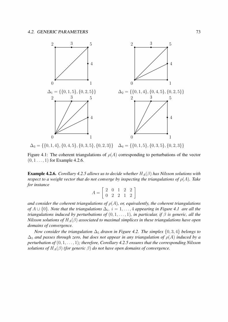
4.2. GENERIC PARAMETERS 73
b
0b
1
b 4
b5
b
3b
2
b
0b
1
b 4
b5
b
3b
2
∆1 = {{0, 1, 5}, {0, 2, 5}} ∆2 = {{0, 1, 4}, {0, 4, 5}, {0, 2, 5}}
b
0b
1
b 4
b5
b
3b
2
b
0b
1
b 4
b5
b
3b
2
∆3 = {{0, 1, 4}, {0, 4, 5}, {0, 3, 5}, {0, 2, 3}} ∆4 = {{0, 1, 5}, {0, 3, 5}, {0, 2, 3}}
Figure 4.1: The coherent triangulations of ρ(A) corresponding to perturbations of the vector(0, 1 . . . , 1) for Example 4.2.6.
Example 4.2.6. Corollary 4.2.5 allows us to decide whether HA(β) has Nilsson solutions withrespect to a weight vector that do not converge by inspecting the triangulations of ρ(A). Takefor instance
A =
[2 0 1 2 20 2 2 1 2
]and consider the coherent triangulations of ρ(A), or, equivalently, the coherent triangulationsof A ∪ {0}. Note that the triangulations ∆i, i = 1, . . . , 4 appearing in Figure 4.1 are all thetriangulations induced by perturbations of (0, 1, . . . , 1), in particular, if β is generic, all theNilsson solutions of HA(β) associated to maximal simplices in these triangulations have opendomains of convergence.
Now consider the triangulation ∆5 drawn in Figure 4.2. The simplex {0, 3, 4} belongs to∆5 and passes through zero, but does not appear in any triangulation of ρ(A) induced by aperturbation of (0, 1, . . . , 1); therefore, Corollary 4.2.5 ensures that the corresponding Nilssonsolutions of HA(β) (for generic β) do not have open domains of convergence.
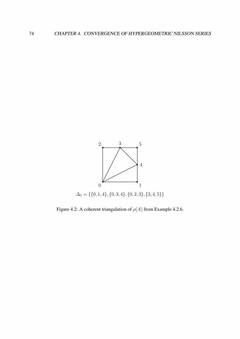
74 CHAPTER 4. CONVERGENCE OF HYPERGEOMETRIC NILSSON SERIES
b
0b
1
b 4
b5
b
3b
2
∆5 = {{0, 1, 4}, {0, 3, 4}, {0, 2, 3}, {3, 4, 5}}
Figure 4.2: A coherent triangulation of ρ(A) from Example 4.2.6.
Chapter 5
Laurent A-hypergeometric solutions andresidues
In this chapter we study Laurent A-hypergeometric series when A is a Cayley configurationA = Cayley(A1, A2) with A1 and A2 subsets of Z2 (see Definition 2.2.1). This configurationis associated to two polynomials f1 and f2 in two variables. This generalizes Example 5.3.4, inwhich we had only one configuration in {1} × Z. We also give several definitions and resultswhich will lead us to the definition and properties of special Laurent A-hypergeometric seriesin terms of combinatorially defined residues. These residues will be the main characters inChapter 6.
Section 5.1 summarizes the basics of A-hypergeometric Laurent series. These are a spe-cial case of logarithm-free hypergeometric series, treated in Section 3.4, but assuming that theparameters β are integer. We study in Section 5.2 the minimal regions that may appear in thecase A = Cayley(A1, A2) and a parameter γ = (−1,−1,−m) with m ∈ Z2. In Section 5.3we introduce local residues associated to Cayley configurations and show that they are specialsolutions for these configurations. The Gel’fond-Khovanskii’s method for the computation ofglobal residues on the torus is presented in Section 5.4. This method will be useful to proveTheorem 6.2.2. Theorem 5.5.2 in Section 5.5 imposes a necessary condition for the algebraicityof A-hypergeometric Laurent series.
5.1 A-hypergeometric Laurent series
Let A = {a1, . . . , an} ⊆ Zd be a regular configuration. As before, we assume, without loss ofgenerality, that the points of A are all distinct and that they span Zd.
We consider the C-vector space:
S =
{∑v∈Zn
cvxv ; cv ∈ C
}
of formal Laurent series in the variables x1, . . . , xn. The matrix A defines a Zd-valued gradingin S by
deg(xv) := A · v ; v ∈ Zn . (5.1)
75
76 CHAPTER 5. LAURENT A-HYPERGEOMETRIC SOLUTIONS AND RESIDUES
We will say that Φ ∈ S is an A-hypergeometric Laurent series of degree β (or Laurent solutionof HA(β)) if it is annihilated by HA(β).
Remark 5.1.1. By [PST05, Proposition 5], if a hypergeometric Laurent series has a non trivialdomain of convergence, then its exponents must lie in a strictly convex cone.
Given β ∈ Zd, consider the fiber
Mβ := {v ∈ Zn : A · v = β}.Recall that for any vector v ∈ Zn we define its negative support as:
nsupp(v) := {i ∈ {1, . . . , n} : vi < 0}, (5.2)
and given I ⊂ {1, . . . , n}, we let r(I,β) = {v ∈Mβ : nsupp(v) = I}. We call r(I,β) a region inMβ .
Definition 5.1.2. We say that r(I,β) is a minimal region if r(I,β) 6= ∅ and r(J,β) = ∅ for J ( I .We write rI instead of r(I,β) is it is clear by the context.
Given a minimal region rI = r(I,β) we let
ΦβrI
(x) :=∑
u∈r(I,β)
(−1)∑i∈I ui
∏i∈I(−ui − 1)!∏
j 6∈I(uj)!xu . (5.3)
Given a weight w ∈ Rn, ε > 0 and ν1, . . . , νn−d a Z-basis of the lattice M = {v ∈ Zn :A · v = 0} satisfying 〈w, νi〉 > 0 for all i = 1, . . . , n− d, we recall from Subsection 1.4.3, thedefinition of the open set:
Uw,ε = {x ∈ Cn | |xνi | < εi for i = 1, . . . , n− d} . (5.4)
Definition 5.1.3. We will denote by rw the collection of minimal regions r(I,β) for which theinner product with w is bounded below and the minimum is attained at a unique point.
The following theorem shows the importance of the Laurent series defined in (5.3).
Theorem 5.1.4. Let A ⊂ Zd and β ∈ Zd as before and w ∈ Rn such that rw is non-empty.Then:
(i) For ε sufficiently small, the open set Uw,ε of the form (5.4) is a common domain of con-vergence of all Φβ
rIwith rI = r(I,β) ∈ rw and
(ii) These ΦβrI
are a basis of the vector space of A-hypergeometric Laurent series of degree βconvergent in Uw,ε.
Proof. First note that the series ΦβrI
is a constant multiple of the Gamma series φv from (3.13).Here v is the element of rI where the inner product 〈w, ·〉 reaches its minimum. In fact,
ΦβrI
= (−1)∑i∈I vi
∏i∈I(−vi − 1)!∏
j 6∈I(vj)!· φv. (5.5)
Considering that in the regular case formal solutions coincide with holomorphic solutions,the proof of the theorem follows from Proposition 3.4.2 and Theorem 3.4.3. Theorem 1.3.16and Subsection 1.4.3 clarify convergence issues.
5.1. A-HYPERGEOMETRIC LAURENT SERIES 77
We can deduce from Theorem 5.1.4 and Remark 5.1.1 an equivalent characterization of rw:it is the collection of those regions r(I,β) which are contained in the intersection of a half-space{v ∈ Rn : 〈w, v〉 ≥ λ, λ ∈ R} with a strictly convex cone.
Definition 5.1.5. We call the series ΦβrI
, for rI ∈ rw minimal, canonical Laurent A-hypergeo-metric series in the direction of w (see Section 3.4 and Definition 1.3.17).
Example 5.1.6. Recall from Example 1.1.4 that the roots of the generic polynomial x2t2 +
x1t+x0 are solutions of an A-hypergeometric system with integer parameters. We can expressthese roots as Laurent series in the variables x0, x1, x2. In fact, developing the square root weobtain:
ρ1 =−x1 + (x2
1 − 4x0x2)1/2
2x2
= − x1
2x2
+
(x1
2x2
−∞∑k=0
1
k + 1
(2k
k
)xk2x
k+10
x2k+11
), (5.6)
ρ2 =−x1 − (x2
1 − 4x0x2)1/2
2x2
= − x1
2x2
−(x1
2x2
−∞∑k=0
1
k + 1
(2k
k
)xk2x
k+10
x2k+11
). (5.7)
For A and β as in Example 1.1.4, the only subsets of {0, 1, 2} such that the correspondingregions are minimal are {1} and {2} with r{1} = {(1 + k,−2(k + 1), k), k ∈ N0} and r{2} ={(0, 1,−1)}. Note that
ρ1 = −Φβr{1}
and ρ2 = −Φβr{2}− Φβ
r{1}. (5.8)
and that both r{1} and r{2} belong to rw for any w = (w0, w1, w2) ∈ R3 such that w0 + w2 >2w1. Moreover, there are no Laurent series in the direction of w for w not satisfying thiscondition.
Remark 5.1.7. Let Φ a Laurent solution of HA(β) in the direction of w. This implies, byTheorem 5.1.4 that
Φ =∑rI∈rw
kIΦβrI
(5.9)
with kI ∈ C and the series Φ converges in Uw,ε. In particular 〈w, u〉 ≥ 0 for all u ∈ rI ∈ rw.If we consider another weight vector w′ such that 〈w′, u〉 ≥ 0 for all u ∈ rI ∈ rw′ ,
according to 5.1.4(ii), we obtain another expansion of Φ converging in an open set Uw′,ε′ .These two expansions have to coincide. In fact, the minimal regions appearing in both haveto belong to rw and rw′ simultaneously, otherwise there would be elements in the support of Φwith negative inner product either with w or w′, contradicting the assumptions. Therefore weobtain a unique expansion converging in Uw,ε ∩Uw′,ε′ .
The following Proposition is an easy calculation.
Proposition 5.1.8. If α ∈ Nn then the derivative ∂α of a canonical Laurent A-hypergeometricseries with homogeneity β is a canonical Laurent A-hypergeometric series with homogeneityβ − A · α.
Since anA-hypergeometric series of degree β satisfies d independent homogeneity relationsit may be viewed as a function of n − d variables. To make this more precise we use a Galedual {b1, . . . , bn} ⊂ Zn−d of the configuration A (see Definition 2.1.1).
78 CHAPTER 5. LAURENT A-HYPERGEOMETRIC SOLUTIONS AND RESIDUES
Remark 5.1.9. (i) Our definition of Gale dual depends on the choice of a basis of M0 =kerZ(A); this amounts to an action of GL(n− d,Z) on the configuration B.
(ii) B is primitive, i.e., if δ ∈ Zn−d has relatively prime entries then so does Bδ. Thisfollows from the fact that if rv ∈ M0 for r ∈ Z and v ∈ Zn then v ∈ M0. Equivalently, therows of B span Zn−d.
(iii) The regularity condition on A is equivalent to the requirement thatn∑j=1
bj = 0. (5.10)
(iv) A is not a pyramid if and only if none of the vectors bj vanishes.
As we saw in previous chapters, given v ∈ Mβ , and the choice of a Gale dual B we mayidentify Mβ
∼= Zn−d by u ∈Mβ 7→ µ ∈ Zn−d with
u = v + µ1ν1 + · · ·+ µn−dνn−d.
In particular, ui < 0 if and only if `i(µ) < 0, where
`i(µ) := 〈bi, µ〉+ vi. (5.11)
The linear forms in (5.11) define a hyperplane arrangement oriented by the normals bi and eachminimal region r(I,β) corresponds to the closure of a certain connected components cI in thecomplement of this arrangement.
Let ΦβrI
(x) as in (5.3). We can also write for v ∈Mβ
ΦβrI
(x) = xv∑
µ∈cI∩Zn−d
∏i∈I(−1)`i(µ)(−`i(µ)− 1)!∏
j 6∈I `j(µ)!xBµ . (5.12)
Settingyj = xνj , j = 1, . . . , n− d, (5.13)
we can now rewrite, the series (5.3) in the coordinates y as ΦβrI
(x) = xvϕcI (y), where
ϕcI (y) :=∑
µ∈cI∩Zn−d
∏`i(µ)<0(−1)`i(µ)(−`i(µ)− 1)!∏
`j(µ)>0 `j(µ)!ym . (5.14)
Moreover, since changing v ∈ Mβ only changes (5.3) by a constant, we can assume that inorder to write (5.14) we have chosen v ∈ r(I,β) and this guarantees that −vi − 1 > 0 for i ∈ Iand vj ≥ 0 for j 6∈ I .
If F (x) is an A-hypergeometric function of degree β, then ∂j(F ) = ∂F/∂xj is A-hyper-geometric of degree β − aj . In terms of the hyperplane arrangement in Rn−d this has the effectof changing the hyperplane {〈bj, ·〉+ vj} to the hyperplane {〈bj, ·〉+ vj − 1}.
The cone of parameters
E = EA :=
{d+2∑i=1
λiai : λi ∈ R, λi < 0
}(5.15)
is called the Euler-Jacobi cone ofA. We note that if β ∈ E then β−aj ∈ E for all j = 1, . . . , n.We also recall the following result of Saito, Sturmfels and Takayama [SST00, Corollary
4.5.13], which we will use in the following sections:
5.2. MINIMAL REGIONS AND MINKOWSKI SUM 79
Theorem 5.1.10. If F is an A-hypergeometric function of degree β ∈ E then, for any j =1, . . . , n, ∂j(F ) = 0 if and only if F = 0.
In particular, all non-zero A-hypergeometric functions F whose degree lies in the Euler-Jacobi cone are stable; that is, no partial derivative ∂αF vanishes.
5.2 Minimal regions and Minkowski sum
We consider the Cayley configuration A = Cayley(A1, A2) given by the lattice points
A1 = {α1, . . . , αr} ⊂ Z2
A2 = {β1, . . . , βs} ⊂ Z2
with r, s > 1, that is, corresponding to the bivariate polynomials
f1(t1, t2) = x1tα1 + . . .+ xrt
αr (5.16)
andf2(t1, t2) = xr+1t
β1 + . . .+ xr+stβs . (5.17)
We set n = r + s. The corresponding integer matrix is
A =
1 . . . 1 0 . . . 00 . . . 0 1 . . . 1α1 . . . αr β1 . . . βs
∈ Z4×n. (5.18)
As always, we assume that ZA = Z4, or equivalently that ZA1 + ZA2 = Z2. Denote by P1 theconvex hull of A1, P2 the convex hull of A2 and by P1 +P2 the Minkowski sum of both, whichhas dimension two.
In this section we study the Laurent solutions of the A-hypergeometric system HA(γ) withparameter
γ = (−1,−1,−m), m ∈ Z2. (5.19)
To that end, in this section we inspect which are the minimal regions rI = r(I,γ) (cf. Definition5.1.2). Let A be as in (5.18) and γ as in (5.19). Our first observation is the following lemma.
Lemma 5.2.1. There are no minimal regions rI with I ⊂ {1, . . . , r} or I ⊂ {r+ 1, . . . , r+ s}.
Proof. This is clear since for any u ∈ Rn such that A · u = γ we have that
r∑i=1
ui =s∑j=1
ur+j = −1
Hence the first case to study possible minimal regions rI is when I = {i0, j0} with i0 ∈{1, . . . , r} and j0 ∈ {r + 1, . . . , r + s}. These regions are related with the points αi0 + βj0 ∈P1 + P2 and their occurrence will depend on m ∈ Z2. We need the following definition:
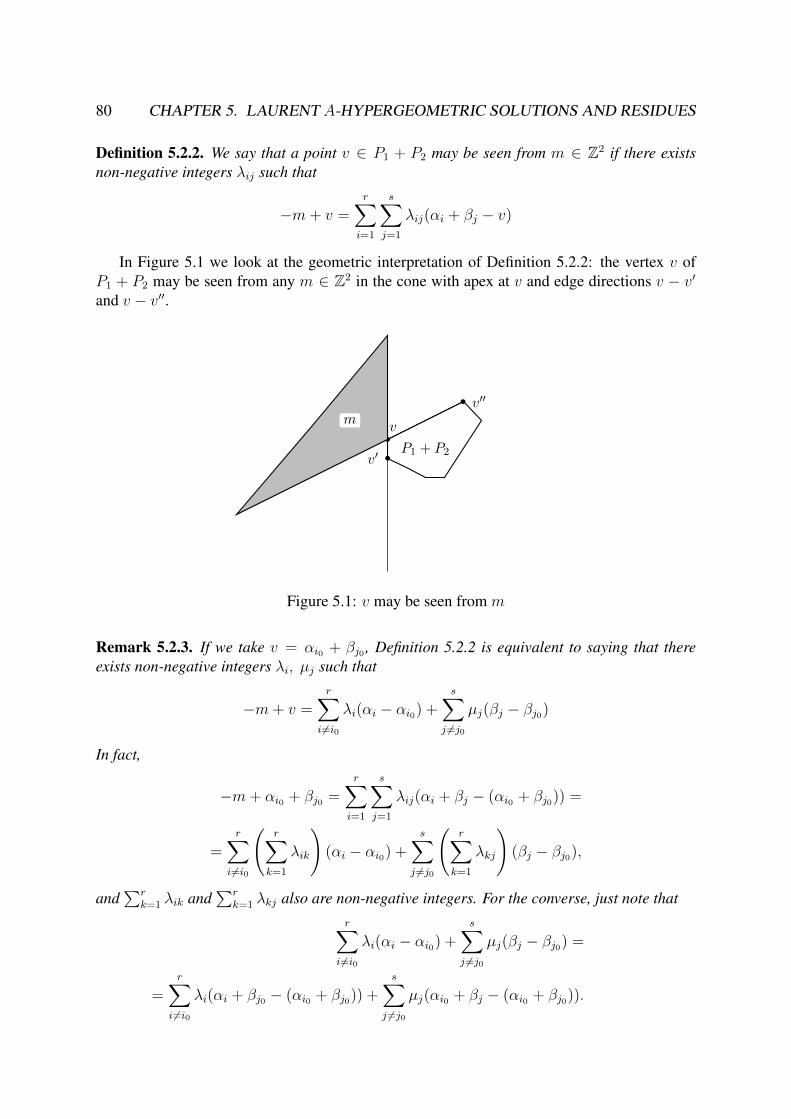
80 CHAPTER 5. LAURENT A-HYPERGEOMETRIC SOLUTIONS AND RESIDUES
Definition 5.2.2. We say that a point v ∈ P1 + P2 may be seen from m ∈ Z2 if there existsnon-negative integers λij such that
−m+ v =r∑i=1
s∑j=1
λij(αi + βj − v)
In Figure 5.1 we look at the geometric interpretation of Definition 5.2.2: the vertex v ofP1 + P2 may be seen from any m ∈ Z2 in the cone with apex at v and edge directions v − v′and v − v′′.
bv′bv
b v′′
m
P1 + P2
Figure 5.1: v may be seen from m
Remark 5.2.3. If we take v = αi0 + βj0 , Definition 5.2.2 is equivalent to saying that thereexists non-negative integers λi, µj such that
−m+ v =r∑
i 6=i0λi(αi − αi0) +
s∑j 6=j0
µj(βj − βj0)
In fact,
−m+ αi0 + βj0 =r∑i=1
s∑j=1
λij(αi + βj − (αi0 + βj0)) =
=r∑
i 6=i0
(r∑
k=1
λik
)(αi − αi0) +
s∑j 6=j0
(r∑
k=1
λkj
)(βj − βj0),
and∑r
k=1 λik and∑r
k=1 λkj also are non-negative integers. For the converse, just note thatr∑
i 6=i0λi(αi − αi0) +
s∑j 6=j0
µj(βj − βj0) =
=r∑
i 6=i0λi(αi + βj0 − (αi0 + βj0)) +
s∑j 6=j0
µj(αi0 + βj − (αi0 + βj0)).

5.2. MINIMAL REGIONS AND MINKOWSKI SUM 81
Remark 5.2.4. From Definition 5.2.2 and Figure 5.1 it is clear that no vertex of P1 +P2 is seenfrom a different vertex of P1 + P2.
Now we can express how this geometric-arithmetic property ofm seeing a point determinesthe occurrence of the regions r{i0,j0}.
Lemma 5.2.5. Let m ∈ Z2. Then the region r{i0,j0} is non-empty if and only if the pointαi0 + βj0 ∈ P1 + P2 may be seen from m.
Proof. For simplicity we assume i0 = j0 = 1. Suppose that there exists a point u ∈ Zr+s suchthat A · u = γ and u1 < 0, ur+1 < 0 and uj ≥ 0 for other j. Then we have
u1 + . . .+ ur = −1,
ur+1 + . . .+ rr+s = −1 and
−m =r∑i=1
uiαi +s∑j=1
ur+jβj.
Combining these three equations we obtain
−m+ α1 + β1 =r∑i=1
ui(αi − α1) +s∑j=1
ur+j(βj − β1) (5.20)
with u2, . . . , ur, ur+2, . . . , ur+s ≥ 0, then by Remark 5.2.3 we obtain that α1 + β1 ∈ P1 + P2
may be seen from m. For the converse just step backwards.
According to Lemma 5.2.5, we can consider different cases of m ∈ Z2 in order to establishwhich minimal regions occur for A and γ. Note that if v = αi0 + βj0 ∈ (P1 + P2)◦, then it isgeometrically clear that any m ∈ Z2 sees the point v and only arithmetic issues may imply thatv be not seen from m, but this never happen, see Corollary 5.2.9.
To study regions corresponding to vertices, we state the following lemma.
Lemma 5.2.6. Let m ∈ Z2 and αi0 + βj0 ∈ P1 + P2 such that αi0 + βj0 is seen from m. Ifαi0 + βj0 is a vertex of P1 + P2 then the region r{i0,r+j0} is finite.
Proof. Assume again i0 = 1, j0 = 1. Note that, being α1 + β1 a vertex, there exists a linearfunctional ξ such that
ξ(α1 + β1) < ξ(αi + βj) for i 6= 1 or j 6= 1.
Hence, if
−m+ α1 + β1 =r∑i=2
ui(αi − α1) +s∑j=2
ur+j(βj − β1) =
=r∑i=2
ui[(αi + β1)− (α1 + β1)] +s∑j=2
ur+j[(α1 + βj)− (α1 + β1)],

82 CHAPTER 5. LAURENT A-HYPERGEOMETRIC SOLUTIONS AND RESIDUES
where ui, ur+j ≥ 0 for all i, j, we have
r∑i=2
uihi +s∑j=2
ur+jkj = ξ(−m+ α1 + β1)
where hi and ki are positive real numbers. Since ui, ur+j are non-negative integers, theirpossible values are bounded and the region with support {1, r + 1} is a bounded minimalregion.
Remark 5.2.7. It can be easily seen that
m ∈ (P1 + P2)◦ if and only if γ = (−1,−1,−m) ∈ E ,
where E is the Euler-Jacobi cone defined in (5.15).
The following results relates supports of vectors in the kernel of the Cayley configurationA with interior lattice points in the Minkowski sum A1 + A2.
Proposition 5.2.8. Fix i ∈ {1, . . . , r}, j ∈ {1, . . . , s}. The following conditions are equivalent:
1. There exists ` = n − 4 linearly independent vectors u(1), . . . , u(`) ∈ kerZ(A) withnsupp(u(i)) = {i, r + j}.
2. αi + βj ∈ (P1 + P2)◦.
3. The minimal region r({i,r+j},(−1,−1,−(αi+βj)) has a recession cone of maximal dimension.
4. There exists m ∈ Z2 such that r({i,r+j},γ) with γ as in (5.19) has a recession cone ofmaximal dimension.
Proof. Assume that 1. holds and let m = αi + βj . Then, γ = A.(−ei − er+j) and so theregion r({i,r+j},(−1,−1,−(αi+βj)) is non empty. Since (−ei − er+j) + u(k) ∈ r({i,r+j},γ) for anyk = 1, . . . , `, it follows that the recession cone is of maximal dimension, proving 3. Item 3.clearly implies 4., which in turns implies 1., as the difference of any two vectors in r({i,r+j},γ)
lies in the kernel of A.We now see the equivalence of items 2 and 3. Let αi + βj ∈ (P1 + P2). If the point lies in
(P1+P2)◦, then γ = (−1,−1, (αi+βj)) lies in the Euler-Jacobi cone and so any minimal regionhas maximal dimension recession cone If instead αi+βj lies in the boundary of P1+P2, let η bean inner normal vector such that 〈η, αi+βj〉 = cη is minimal and 〈η, v〉 ≥ cη for all v ∈ P1+P2.We denote by F the corresponding face and F1, F2 the faces of P1, P2 such that F = F1 + F2,Any vector in rI , is a Z-linear combination of the vectors (1, 0, αk), k = 1, . . . , r and (0, 1, β`)with coefficients (u1, . . . , ur+s) which non negative coefficients except from Ui, ur+j ∈ Z<0.Moreover, the sum of the first r and last s coordinates equal to −1. We then have
αi + βj =∑k 6=1
uk((αk + βj)− (αi + βj) +∑`6=j
u`+r((αi + β`)− (αi + βj)).
As,∑
k 6=i ui = 0,∑
` 6=j u`+r = 0, we can argue as in Lemma 5.2.6. We take the inner producton both sides with η and using the positivity, we deduce that uk = 0 if αk 6∈ F1, u` = 0 ifβell 6∈ F2. Therefore, rI cannot be full dimensional.

5.3. RESIDUES AND CAYLEY CONFIGURATIONS 83
Corollary 5.2.9. If αi0 + βj0 is an interior point of P1 + P2 then it may be seen from anym ∈ Z2.
Proof. Given m ∈ Z2, our assumption that ZA = Z4 ensures that we can always take v ∈ Znsuch thatA ·v = (−1,−1,−m). By the first item in Proposition 5.2.8, there exists u ∈ kerZ(A)with nsupp(u(i)) = {i, r + j} and all coordinates ui are non zero. Then, for any sufficientlybig λ ∈ N it holds that A · (λu + v) = (−1,−1,−m) and nsupp(λu + v) = {i0, r + j0}. Wededuce from Lemma 5.2.5 that v may be seen from m.
5.3 Residues and Cayley configurations
In this section we introduce local and global residues and show that they satisfy a particular A-hypergeometric system. The local Grothendieck residue associated with a family of k-variateLaurent polynomials f1, . . . , fk with an isolated zero at a point ξ, is defined by
Resf,ξ(h) =1
(2πi)k
∫Γξ(ε)
h(t)
f1(t) . . . fk(t)
dt1t1∧ . . . ∧ dtk
tk(5.21)
where Γξ(ε) is the real k-cycle Γξ(ε) = {|fi(t)| = εi} oriented by the k-form d(arg(f1)) ∧. . . ∧ d(arg(fk)). For almost every ε = (ε1, . . . , εk) in a neighborhood of the origin, Γξ(ε) issmooth and by Stokes’ Theorem the integral (5.21) is independent of ε. Note that this definitionmakes sense as long as h is holomorphic in a neighborhood of ξ. If ξ is a simple zero then thetoric Jacobian
JTf (ξ) = det
(tj∂fi∂tj
(ξ)
)is non-zero and
Resf,ξ(h) =h(ξ)
JTf (ξ). (5.22)
This identity follows from the change of coordinates yi = fi(t) and iterated integration.Assuming that the set V of common zeros of f1, . . . , fk in the torus T = (C∗)k is finite, we
can define the global residue as the sum of local residues:
Resf1,...,fk(h) =∑ξ∈V
Resf,ξ(h). (5.23)
where h is holomorphic around each ξ ∈ V (for instance h = h1
h2with h1, h2 polynomials with
h2(ξ) 6= 0 for each ξ ∈ V ).Residues are solutions of certainA-hypergeometric systems. Fix k configurations of integer
points, Ai = {αi1, . . . , αi|Ai|} ⊂ Zk for i = 1, . . . , k and denote
x = (xα11, . . . , xα1
|A1|, . . . , xαk1 , . . . , xαk|Ak|
), t = (t1, . . . , tk).

84 CHAPTER 5. LAURENT A-HYPERGEOMETRIC SOLUTIONS AND RESIDUES
Let f1(x; t), . . . , fk(x; t) be k-variate polynomials with these exponents and |A1| + · · · + |Ak|indeterminate coefficients
fi(x; t) =
|Ai|∑l=1
xαiltαil ; i = 1, . . . , k. (5.24)
Then, for generic values of the coefficients x, f1, . . . , fk will have a finite set V of commonzeros in the torus.
Let n = |A1| + · · · + |Ak| and d = 2k. Recall that the Cayley configuration A =Cayley(A1, . . . , Ak) associated with A1, . . . , Ak is the configuration in Zd defined by
A = {e1}× A1 ∪ · · · ∪ {ek}×Ak. (5.25)
We have the following proposition, whose proof can be found in [Dic04, Proposition 3.4].
Proposition 5.3.1. For any m ∈ Zk, the local residue
Resmf,ξ := Resf,ξ(tm) (5.26)
where tm = tm11 . . . tmkk and ξ ∈ V is anA-hypergeometric algebraic function of the coefficients
x of f1, . . . , fk with homogeneity
γ = (−1, . . . ,−1,−m1, . . . ,−mk) ∈ Zd.
Consequently, the global residue (5.23) is a rational A-hypergeometric function with the samehomogeneity.
For q ∈ Nn and i = 1, . . . , k denote by qi = (0, . . . , 0, q|Ai−1|+1, . . . , q|Ai−1|+|Ai|, 0, . . . , 0).The following proposition follows easily by differentiating under the integral sign.
Proposition 5.3.2. Let q ∈ Nn then
∂q (Resf,ξ(tm)) = (−1)|q|
n∏i=1
(|qi| − 1)!Resf ,ξ(tm) (5.27)
where f denotes the collection of polynomials f |q1|, . . . , f |q
n| and
m = m+n∑i=1
|Ai|∑j=1
q|Ai−1|+jαij,
where |A0| is understood as 0.
Let A1, . . . , Ak be k configurations in Zk. As usual, we denote by A1 + · · · + Ak theirMinkowski sum {αij1 + · · ·+ αijk, α
ijl ∈ Ai}.
The following result about vanishing of global residues, due to A. Khovanskii [Kho78], isthe sparse version of the classical Euler-Jacobi Theorem.
Theorem 5.3.3. Let f1, . . . , fk be generic polynomials with coefficients in A1, . . . , Ak. For anyLaurent polynomial h with support contained in the interior of the convex hull ofA1 + · · ·+Ak,the global residue Resf1,...,fk(h) is equal to 0.

5.4. A-HYPERGEOMETRIC SOLUTIONS ASSOCIATED TO A VERTEX 85
Example 5.3.4. Consider the 1-dimensional Cayley configuration
A =
(1 1 . . . 1 10 k1 . . . km `
)and let
f(x; t) := x0 + xk1tk1 + · · ·+ xkmt
km + x`t`
denote the polynomial with exponents 0, k1, . . . , km, ` and indeterminate coefficients. The pow-ers ρs(x), s ∈ Z of the roots of f(x; t), viewed as functions of the coefficients, are algebraicsolutions of the A-hypergeometric system with exponent (0,−s) and the total sum
ps(x) := ρs1(x) + · · ·+ ρsd(x)
is then a rational solution with the same exponent. Similarly, one can show that the localresidues
Resρ(x)
(tb
fa(x; t)
dt
t
), a, b ∈ Z; a ≥ 1
give algebraic solutions with exponent (−a,−b) and, again, the total sum of residues is arational solution. In [CDD99] a family of algebraic A-hypergeometric functions is defined interms of the roots of the polynomial f(x; t). These functions are used to construct a basis ofthe space of solutions for any integer parameter.
5.4 A-hypergeometric solutions associated to a vertex
In this section we show that canonicalA-hypergeometric series with homogeneity γ as in (5.19)corresponding to minimal regions associated with a vertex αi0 + βj0 of P1 + P2, are residuesassociated to f1 and f2 as defined in (5.16),(5.17).
5.4.1 The Gelfond-Khovanskii method for calculating residues
We say that two lattice polygones Q1 and Q2 are developed if no edge of Q1 is allowed to beparallel to an edge of Q2. This implies that each edge E of Q1 + Q2 is either a translate of anedge of Q1 (“a 1–edge”) or a translate of an edge of Q2 (“a 2–edge”). Along this section wesuppose that Q1 and Q2 are developed.
Given h ∈ C[t1, t−11 , t2, t
−12 ], let Resg1,g2(h) as in (5.23), for k = 2. In [GK96], the follow-
ing method to calculate Resg1,g2(h) is introduced, assuming that Qi := New(gi), i = 1, 2, aredeveloped.
To each vertex v = (v1, v2) of Q1 + Q2 we assign a combinatorial coefficient kv ∈{−1, 0,+1} according to the following rule:
Let E1, E2 be the two edges of Q1 +Q2 adjacent to v in counterclockwise order. We set
kv :=
−1 if E1 is a 1 -edge and E2 is a Q2-edge,+1 if E1 is a 2-edge and E2 is a Q1 -edge,0 if E1 and E2 are both Q1 -edges or both Q2-edges.
(5.28)
We call the coefficient kv, combinatorial Khovanskii coefficient of v.
86 CHAPTER 5. LAURENT A-HYPERGEOMETRIC SOLUTIONS AND RESIDUES
Let av · tv11 t
v22 be the extreme term of g1 · g2 corresponding to v. We define L(v) to be the
formal Laurent series
L(v) =1
av · tv11 t
v22
·∞∑n=0
(1− g1(t1, t2) · g2(t1, t2)
av · tv11 t
v22
)n. (5.29)
Denote by Rv,g1,g2(h) the constant term of h · L(v). Then, the theorem of Gel’fond and Kho-vanskii states:
Theorem 5.4.1. With the previous notation,
Resg1,g2(h) =∑
v a vertex of Q1+Q2
kv ·Rv,g1,g2(h). (5.30)
5.4.2 Laurent polynomial solutions
Now, we can combine the Gelfond-Khovanskii method with the notion of m “seeing” v fromDefinition 5.2.2. Take f1, f2, P1 and P2 as in the beginning of Section 5.2, with P1 and P2
developed.
Proposition 5.4.2. Let m ∈ Z2 and v a vertex of P1 +P2, then Rv,f1,f2(tm) = 0 if v is not seenfrom m.
Proof. It is clear from Definition 5.2.2 and Equation (5.29) that if v is not seen from m, noconstant term appears in the product tm · L(v).
Theorem 5.4.3. Let m ∈ Z2 and v = αi0 + βj0 ∈ P1 + P2 a vertex such that v is seenfrom m. Then Resv,f1,f2(tm) agrees with the canonical hypergeometric Laurent polynomialcorresponding to the minimal region r{i0,j0}.
Proof. Suppose that v = α1 +β1 so that avtv = x1xr+1tα1+β1 . Let xu be a monomial appearing
in Rv(tm) with coefficient Cu. Then, we have that all exponents uk are non-negative except
u1, ur+1 which are strictly negative and
u1 = −1− u2 − · · · − ur and ur+1 = −1− ur+2 − · · · − ur+s.
As usual, let us denote by u+, the non-negative entries of u and consider the derivative
∂u+ ·Rv(tm)
We claim that∂u+ ·Rv(t
m) = Cu (∏uj>0
uj!) xu11 · xur+1
r+1 .
Indeed, suppose u ∈ Zr+s is such that A · u = γ and nsupp(u) = {1, r + 1}. Then ∂u+xu = 0unless u+ ≥ u+, in the sense that the entries of u+ are greater than or equal than those of u+.Suppose then that there exists such u with u+ ≥ u+. It follows that
u1 ≤ u1 ; ur+1 ≤ ur+1.
5.5. A NECESSARY CONDITION FOR THE ALGEBRAICITY 87
But then the vector u − u ∈ kerZA has negative support contained in {1, r + 1}. It followsthat, since the region is bounded by Lemma 5.2.6, we must have u = u and there is only oneterm left.
On the other hand, we have that ∂u+ · Rv(tm) is the zero order coefficient in the expansion
of
∂u+
(tm
x1xr+1tα1tβ1(f1/x1tα1)(f2/xr+1tβ1)
)=
(−1)a+b a! b! tm
x1xr+1tα1tβ1(f1/x1tα1)a(f2/xr+1tβ1)b,
where a = u2 + · · ·+ ur = −u1 − 1, b = ur+2 + · · ·+ ur+s = −ur+1 − 1 and
m = m+r∑i=2
ui αi +s∑j=2
ur+j βj.
Now, note that since xu was a term in Rv(tm) we have
−m+ α1 + β1 =r∑i=2
ui (αi − α1) +s∑j=2
ur+j (βj − β1)
and therefore−m+ (a+ 1)α1 + (b+ 1)β1 = 0.
Hence, the zero order coefficient in the expansion is simply:
(−1)a+b a! b!
xa+11 xb+1
a+1
.
Comparing the two expressions we get:
Cu =(−1)a+b a! b!∏
uj>0 uj!.
This implies that Rv(tm) is the canonical hypergeometric Laurent polynomial (cf. (5.3)) with
homogeneity γ corresponding to the bounded minimal region r{1,r+1}.
5.5 A necessary condition for the algebraicity of A-hyper-geometric Laurent series
In this section we give a necessary condition for the algebraicity of the canonical Laurent A-hypergeometric series Φγ
rI(cf. (5.3)). We will need the following result proved in [CDR11].
Theorem 5.5.1. The hypergeometric series
u(z) :=∞∑n=0
∏ri=1(pin+ ki)!∏s
j+i(qjn)!zn , ki ∈ N (5.31)

88 CHAPTER 5. LAURENT A-HYPERGEOMETRIC SOLUTIONS AND RESIDUES
is algebraic if and only if s− r = 1 and the factorial ratios
An :=
∏ri=1(pin)!∏sj+i(qjn)!
are integral for every n ∈ N.
Let A ∈ Zn×d and β ∈ Zd and B ∈ Zn×n−d a Gale dual of A with rows b1, . . . , bn. We saythat a canonical series φ(I,β) with unbounded r(I,β) has regular support if there exists an infiniteextremal ray of r(I,β) defined by the vanishing of the linear forms associated to indices K in thecomplement of I , such that for any J ∈ K with cardinality n− d− 1 such that {bi, i ∈ J} arelinearly independent, and any i ∈ I , bi is not in the linear span of those vectors. Any such raywill be called regular.
We then have:
Theorem 5.5.2. Given r(I,β) ∈ rw, if the canonical Laurent A-hypergeometric series ΦβrI
isalgebraic and has regular support, then |I| ≤ d
2.
Proof. By the discussion in Section 5.1 (cf. (5.13) and (5.14) for the notations), it is enough toshow that if the series
ϕcI (y) :=∑
µ∈cI∩Zn−d
∏`i(µ)<0(−1)`i(µ)(−`i(µ)− 1)!∏
`j(µ)>0 `j(µ)!yµ .
is algebraic, then |I| ≤ d2. Note that the number of factorials in the numerator is |I| and the num-
ber of factorials in the denominator is n− |I|. Suppose then that ϕcI (y) is algebraic. Considerthe restriction of ϕcI (y) to an (infinite) regular ray of cI given by `j1(µ) = 0, . . . , `j`(µ) = 0,` ≥ n−d−1. Then this restriction must also be algebraic. But this is a univariate hypergeomet-ric series of the form (5.31) with integral ratios and |I| factorials in the numerator (which areall non trivial by the hypothesis of regular support) and n−|I|−` factorials in the denominator.Then, by Theorem 5.5.1, we have that n− |I| − ` = |I|+ 1 and we conclude that |I| ≤ d
2.
The following example explains the inclusion of the hypothesis of regular support.
Remark 5.5.3. Let A1 = {α1 = (0, 0), α2 = (1, 1)} and A2 = {β1 = (0, 0), β2 = (1, 0), β3 =(0, 1), β4 = (0, 2)}. Note that β3 is an interior point of the edge with vertices β1, β4. Thedimension of a Gale dual configuration to A is two. Take any integer homogeneity in E . Thereis an unbounded minimal region with negative support {1, 4, 5}. Note that b1 and b4 are linearlydependent with b2, and one of the infinite rays of its recession cones is defined by `2 = 0. Therestriction of the associated canonical series Φ to this ray is an algebraic hypergeometricfunction. However, the other infinite ray allows to preclude the algebraicity of Φ.
In the case of Cayley configurations, we obtain the following corollary.
Corollary 5.5.4. Let A be the Cayley configuration in Z2k associated to k configurations inZk. Let γ = (u,−m), with u ∈ Zk<0,m ∈ Zk a homogeneity in the Euler-Jacobi cone E . LetΦI be an algebraic canonical A-hypergeometric Laurent series of homogeneity γ with negativesupport I . If φI has regular support then |I| = k.

5.5. A NECESSARY CONDITION FOR THE ALGEBRAICITY 89
Proof. As γ ∈ E , no minimal region is bounded. We deduce from Theorem 5.5.2 that |I| ≤2k2
= k. On the other side, as the k first entries of γ are negative I needs to “intersect” the indexset of each of the k configurations and so also |I| ≥ k.
90 CHAPTER 5. LAURENT A-HYPERGEOMETRIC SOLUTIONS AND RESIDUES

Chapter 6
Algebraic A-hypergeometric solutions andresidues
We now turn our attention to algebraic solutions of regular A-hypergeometric systems HA(β),with β an integer (resonant) parameter. Rational solutions (which are, in particular, algebraicsolutions) of A-hypergeometric systems have been studied in, e.g., [CDS01, CDR11, CDD99,PST05]. A characterization of A-hypergeometric systems having a full set of algebraic solu-tions is given in [Beu10], using tools from number theory.
In this final chapter we study the algebraic A-hypergeometric Laurent solutions of the Cay-ley configuration A = Cayley(A1, A2) with A1 and A2 subsets of Z2. This configuration isassociated to two polynomials f1 and f2 in two variables. In the case of one univariate poly-nomial with fix monomial support, the algebraic solutions of the associated configuration weredescribed by means of residues in Example 5.3.4. Those residues are defined in terms of theroots of the polynomial, which can in turn be explicitly described in terms of the coherent tri-angulations of the convex hull of the configuration. Here, the coherent mixed subdivisions ofthe Minkowski sum of A1 and A2, studied in Chapter 2, will help us to describe the roots off1 and f2 over which we will add the local residues, to produce algebraic A-hypergeometricLaurent series convergent in explicit open sets.
In section 6.1 we introduce this notion of residues associated to a mixed cell of a coherentmixed subdivision of the Minkowski sum of A1 and A2. In section 6.2, we show how theseresidues can be written in terms of canonical Laurent A-hypergeometric series. This is thecontent of Theorem 6.2.2, a main result in this chapter. We prove in Theorem 6.3.1 of section6.3 that all algebraic solutions for these configurations can be described in terms of residues incase the Cayley configuration associated to A1, A2 has codimension two. Finally, we presentin the last section general conjectures for further study.
6.1 Coherent mixed subdivisions and residues
In [HS95], an algorithm based on coherent mixed subdivision to find the solutions of a polyno-mial system is introduced. We explain it briefly:
Let w ∈ Rn be a generic weight and Πw the coherent mixed subdivision associated to it.
91
92 CHAPTER 6. ALGEBRAIC A-HYPERGEOMETRIC SOLUTIONS AND RESIDUES
Let σ = {i0, i1, j0, j1} ∈ Πw a mixed cell and
fσ1 = xi0tαi0 + xi1t
αi1 , (6.1)
fσ2 = xr+j0tβj0 + xr+j1t
βj1 . (6.2)
Denote Aσ1 = {i0, i1}, Aσ2 = {j0, j1}, so that σ = Aσ1 + Aσ2 . Let
ξσ1 , . . . , ξσvol(σ)
be the roots of fσ1 , fσ2 . Then we can “extend” them to ξ1, . . . , ξvol(σ) roots of f1, f2 such thattheir coordinates are Puiseaux series in x = (x1, . . . , xn). More explicitly, for each i, ξi = ξi(x)is an algebraic function of x such that ξi converges in Uw,ε for ε sufficiently small. Moreover
Lemma 6.1.1. There exists w ∈ w + rowspan(A) such that wt = 0 for t = i, j, k or l andwt > 0 otherwise. Consequently
inw (ξih(x)) = ξσih(x) h = 1, 2, (6.3)
i.e. ξih(x) = ξσih(x) + h.o.t.(x).
Now we use this information to define algebraic solutions to our A-hypergeometric systemHA(γ). Since the functions defining the roots are clearly algebraic, it follows that the localresidue of tm with respect of f1, f2 is also an algebraic function, because generically in x wecan write
Resmf1,f2,ξi(x) := Resf1,f2,ξi(x)(tm) =
ξm1i1 ξ
m2i2
JTf (ξi), (6.4)
and the right-hand side of this equality is clearly algebraic. Thus
Resmσ (x) :=
vol(σ)∑i=1
Resmf1,f2,ξi(x) (6.5)
is an algebraic Laurent A-hypergeometric function in Uw,ε with homogeneity (−1,−1,−m).We call it the local residue relative to the cell σ.
It follows from Theorem 5.3.3 that for anym ∈ (P1 +P2)◦ and any generic weight w ∈ Rn,the residues {Resmσ , σ maximal cell in Πw} satisfy the linear relation∑
σ
Resmσ = 0. (6.6)
Given w ∈ Rn generic and γ ∈ Z4, we denote by Algγ,w the subspace of A-hypergeometricLaurent algebraic series with homogeneity γ that converge in the direction of w.
We then obtain the following Corollary:
Corollary 6.1.2. For generic w ∈ Rn, m ∈ (P1 + P2)◦ and γ = (−1,−1,−m) it holds
Rγ,w := 〈Resmσ , σ a mixed cell in Πw〉 ⊆ Algγ,w. (6.7)
Moreoverdim(Rγ,w) ≤ #(mixed cell in Πw)− 1. (6.8)

6.2. ALGEBRAIC SOLUTIONS AS RESIDUES 93
6.2 Algebraic solutions as residues
In this section we present one of our fundamental result in this chapter: Theorem 6.2.2. wherewe find the expression of the residues associated to cells in a mixed subdivision in terms ofcanonical series solutions.
Notation 6.2.1. Let w ∈ Rn be a generic weight and consider a cell σ ∈ Πw. We will denoteby kσ,v ∈ {1,−1, 0} the combinatorial Khovanskii coefficient of the vertex v ∈ σ (cf. (5.28))associated to fσ1 and fσ2 (cf. (6.1) and (6.2)). HereQ1 = Aσ1 andQ2 = Aσ2 which are developedsince dim(σ) = 2.
Being a Laurent A-hypergeometric series converging in Uw,ε, Theorem 5.1.4 says that thelocal residue relative to the cell σ can be written in terms of the canonical Laurent series Φγ
rIin
the direction of w. The next theorem shows that, for m ∈ (P1 +P2)◦∩Z2, in the correspondingexpansion of Resmσ the only Φγ
rIthat appear are those such that I = {i, j} and rI is a infinite
region corresponding to a point αi + βj ∈ σ ∩ (P1 + P2)◦. Moreover, the coefficients aredetermined.
Theorem 6.2.2. Let w ∈ Rn, m ∈ (P1 + P2)◦ ∩ Z2 and σ a mixed cell in a subdivision Πw
of P1 + P2. Assume that all non empty r(I,(−1,−1,−m) with I{1, . . . , n} ⊂ σ with |I| = 3 areregular supports with regular ray extremal for some weight. Then
Resmσ (x) =∑
kσ,vΦγr{i,j}
(x) (6.9)
where v runs over the points αi + βj ∈ σ ∩ (P1 + P2)◦.
In order to prove Theorem 6.2.2 we will need the following Lemmas.
Lemma 6.2.3. Let w ∈ Rn generic such that σ is mixed cell with σ ⊂ Πw and m ∈ Z2,γ = (−1,−1,−m). In the expansion:
Resmσ =∑rI∈rw
kIΦγrI, (6.10)
the coefficients kI are independent of the choice of m.
Proof. Take m,m′ ∈ Z2. Then there exists q, q′ ∈ Nn such that
∂q(Resmσ ) = ∂q′(Resm
′
σ ).
In fact, by Proposition 5.3.2 it is enough to take q, q′ such that q1 + · · · + qr = q′1 + · · · + q′r,qr+1 + · · ·+ qr+s = q′r+1 + · · ·+ q′r+s and m+
∑ri=1 qiαi +
∑sj=1 qr+jβj = m′ +
∑ri=1 q
′iαi +∑s
j=1 q′r+jβj . This can always be done, because of our hypothesis ZA = Z4.
Taking into account the respective expansions of both functions (cf. Theorem 5.1.4(ii))and interchanging infinite sum with derivative (which is allowed by uniform convergence) weobtain: ∑
rI∈rwkI(m)∂q
(ΦγrI
)=∑rI∈rw
kI(m′)∂q
′(
Φγ′
rI
)
94 CHAPTER 6. ALGEBRAIC A-HYPERGEOMETRIC SOLUTIONS AND RESIDUES
where γ′ = (−1,−1,−m). By Proposition 5.1.8 we obtain the identity:∑rI∈rw
kI(m)(Φγ−AqrI
)=∑rI∈rw
kI(m′)(
Φγ′−Aq′rI
). (6.11)
Let δ = m − Aq = m′ − Aq′. Since the series (ΦδrI
)I are a basis of the space of Laurent A-hypergeometric functions with homogeneity δ, and that, by Theorem 5.1.10 and Remark 5.2.7,all the coefficients kI(m) and kI(m′) appearing in the expansions of Resmσ and Resm′σ respec-tively also appear in (6.11), we conclude that the coefficients kI(m) coincide with kI(m′).
Lemma 6.2.4. Let w ∈ Rn generic such that σ is mixed cell with σ ⊂ Πw. Suppose thatm = αi0 + βj0 ∈ σ ∩ (P1 + P2)◦. Then there exists w such that Πw = Πw and
inw(Resmσ (x)) = Resmfσ1 ,fσ2 = kσ,mx−1i0x−1r+j0
. (6.12)
Proof. Let w as in 6.1.1. Putting fσ1 and fσ1 instead of f1 and f2 as in (6.1) and (6.2) respec-tively, and Aσ1 and Aσ2 instead of P1 and P2 in Theorem 5.4.3 we have that Resmfσ1 ,fσ2 6= 0.Then
inw(Resmσ (x)) =
vol(σ)∑i=1
inw(Resmf1,f2,ξi(x)
)=
vol(σ)∑i=1
inw
(ξmi
JTf (ξi)
)=
vol(σ)∑i=1
inw(ξmi )
inw(JTf (ξi))=
=
vol(σ)∑i=1
(ξσi )m
JTfσ(ξσi )= Resmfσ1 ,fσ2 (6.13)
To see that the last equality in (6.12) holds, we use Theorem 5.4.1 for fσ1 , fσ2 . Name
vhl = αih + βjl , h, l = 0, 1 (note that m = v00). Then we obtain:
Resfσ1 ,fσ2 (tm) =1∑
h,l=0
kσ.vhl(vhl) ·Rvkl(tm). (6.14)
From Remark 5.2.4 and Proposition 5.4.2 we obtain that Rvkl(tm) = 0 if vhl 6= v00 = m. On
the other hand, Rm(tm) = kσ,mx−1i0x−1r+j0
is an easy calculation.
Now we are ready to prove Theorem 6.2.2.
Proof (of Theorem 6.2.2). By Lemma 6.2.3 we write
Resmσ =∑rI∈rw
kIΦrI . (6.15)
We will prove that all the coefficients kI in (6.10) are zero except for those correspondingto I = {i, j} with v = αi + βj ∈ (P1 + P2)◦ ∩ σ, which will be equal to the Khovanskiicombinatorial coefficients kσ,m (see Notation 6.2.1).
First consider a minimal region rI 6= ∅ such that I ( σ. By Lemma 2.2.6 there existsw′ ∈ Rn weight vector such that σ ∈ Πw′ and I * Πw′ . Then ΦrI does not appear in the
6.3. THE CASE N = 6 95
expansion in the direction of w′, that is, the corresponding coefficient is zero. As Resmσ is alsoa Laurent solution with respect to w, both expansions coincide (see Remark 5.1.7). So
Resmσ =∑I ⊂ σrI 6= ∅
kIΦrI . (6.16)
Now we are left with minimal regions rI 6= ∅ such that I ⊆ σ. It is easy to see that if kI 6= 0,then I cannot be the whole of σ, since in this case I is not contained in any other mixed cell andthe correspoding summand cannot be canceled as the Euler Jacobi theorem 5.3.3 asserts. Wediscard all regions rI with |I| = 3 using Corollary 5.5.4 by our hypothesis on these supports.
So we see that the only coefficients that may be distinct to zero are those corresponding toregions rI 6= ∅ with I = {i, j}, with αi + βj ∈ (P1 + P2)◦ ∩ σ. As γ ∈ E , we deduce fromProposition 5.2.8 that αi + βj lies in the interior (P1 + P2)◦ of the Minkowski sum.
Finally we compute the coefficient corresponding to I = {i, j}with αi+βj ∈ (P1+P2)◦∩σ.Assume, by Lemma 6.2.3, thatm = αi+βj . Then Lemma 6.2.4 shows that kσ,mx−1
i x−1r+j appear
in the expansion of Resmσ . But this is a term in the canonical Laurent series Φγr{i,j}
and then thewhole series must appear multiplied by the coefficient kσ,m.
We will show in the next Section that the hypotheses of regularity and extremality of nega-tive supports with cardinality three hold in codimension two if all points αi, βj are vertices.
We obtain the following variant of Theorem 5.3.3.
Corollary 6.2.5. If σ has no vertices in (P1 + P2)◦ and m ∈ (P1 + P2)◦ then Resmσ = 0.
Example 6.2.6. Assume that we have two configurations of dimension one, for instance letA1 = {αi+1 = (i, 0), 0 ≤ i ≤ r − 1} and A2 = {βj+1 = (0, j), 0 ≤ j ≤ s − 1}, r, s ≥ 2.Then, a possible coherent mixed subdivision of A1 +A2 consists of the following s− 1 cells σj ,j = 1, . . . , s − 1, which are all mixed and rectangular, with the four vertices in the boundaryof A1 + A2:
σj = {1, r, j, j + 1}.Then, by Corollary 6.2.5, the sum of the residues Rm
σjover each one of these cells is 0, which
gives new linear relations among them, different from the Euler-Jacobi vanishing condition.As before, denote by f1 = f1(x), f2 = f2(y) polynomials with variable coefficients associatedto A1, A2. These zero residues Rm
σjcorrespond to the sum of the residues over all the points
(a, yj), j = 1, . . . , s− 1, here a is a fixed zero of f1 and yj ranges over all the zeros of f2.
6.3 The case n = 6
In this section we will make a detailed description of algebraic Laurent series solutions of thesystem HA(γ) in terms of residues, in case n = r + s = 6, r, s ≥ 2, which corresponds tonon pyramidal codimension two Cayley configurations. As before γ = (−1,−1,−m) withm ∈ (P1 + P2)◦. In view of Example 6.2.6, we will deal with the following cases: A1, A2 aretwo trinomials with dim(A1) = dim(A2) = 2 or A1 is a binomial and A2 quatrinomial withdim(A2) = 2 and all αi, βj are vertices.
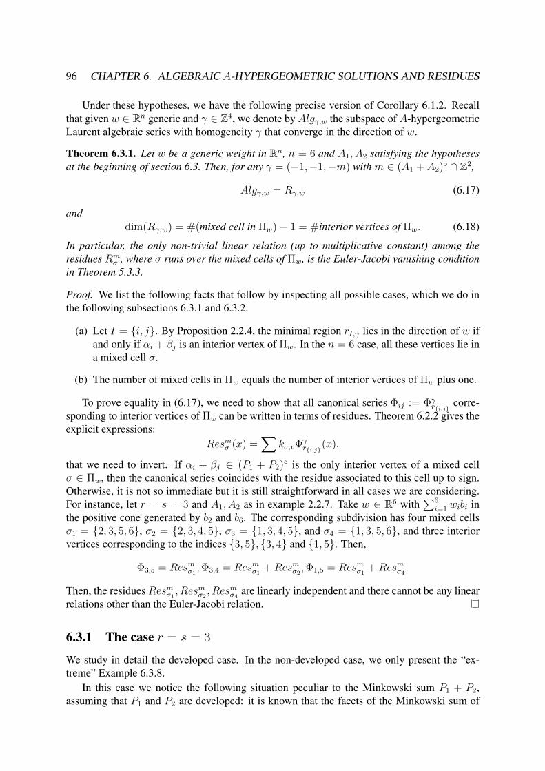
96 CHAPTER 6. ALGEBRAIC A-HYPERGEOMETRIC SOLUTIONS AND RESIDUES
Under these hypotheses, we have the following precise version of Corollary 6.1.2. Recallthat given w ∈ Rn generic and γ ∈ Z4, we denote by Algγ,w the subspace of A-hypergeometricLaurent algebraic series with homogeneity γ that converge in the direction of w.
Theorem 6.3.1. Let w be a generic weight in Rn, n = 6 and A1, A2 satisfying the hypothesesat the beginning of section 6.3. Then, for any γ = (−1,−1,−m) with m ∈ (A1 + A2)◦ ∩ Z2,
Algγ,w = Rγ,w (6.17)
anddim(Rγ,w) = #(mixed cell in Πw)− 1 = #interior vertices of Πw. (6.18)
In particular, the only non-trivial linear relation (up to multiplicative constant) among theresidues Rm
σ , where σ runs over the mixed cells of Πw, is the Euler-Jacobi vanishing conditionin Theorem 5.3.3.
Proof. We list the following facts that follow by inspecting all possible cases, which we do inthe following subsections 6.3.1 and 6.3.2.
(a) Let I = {i, j}. By Proposition 2.2.4, the minimal region rI,γ lies in the direction of w ifand only if αi + βj is an interior vertex of Πw. In the n = 6 case, all these vertices lie ina mixed cell σ.
(b) The number of mixed cells in Πw equals the number of interior vertices of Πw plus one.
To prove equality in (6.17), we need to show that all canonical series Φij := Φγr{i,j}
corre-sponding to interior vertices of Πw can be written in terms of residues. Theorem 6.2.2 gives theexplicit expressions:
Resmσ (x) =∑
kσ,vΦγr{i,j}
(x),
that we need to invert. If αi + βj ∈ (P1 + P2)◦ is the only interior vertex of a mixed cellσ ∈ Πw, then the canonical series coincides with the residue associated to this cell up to sign.Otherwise, it is not so immediate but it is still straightforward in all cases we are considering.For instance, let r = s = 3 and A1, A2 as in example 2.2.7. Take w ∈ R6 with
∑6i=1 wibi in
the positive cone generated by b2 and b6. The corresponding subdivision has four mixed cellsσ1 = {2, 3, 5, 6}, σ2 = {2, 3, 4, 5}, σ3 = {1, 3, 4, 5}, and σ4 = {1, 3, 5, 6}, and three interiorvertices corresponding to the indices {3, 5}, {3, 4} and {1, 5}. Then,
Φ3,5 = Resmσ1,Φ3,4 = Resmσ1
+Resmσ2,Φ1,5 = Resmσ1
+Resmσ4.
Then, the residues Resmσ1, Resmσ2
, Resmσ4are linearly independent and there cannot be any linear
relations other than the Euler-Jacobi relation.
6.3.1 The case r = s = 3
We study in detail the developed case. In the non-developed case, we only present the “ex-treme” Example 6.3.8.
In this case we notice the following situation peculiar to the Minkowski sum P1 + P2,assuming that P1 and P2 are developed: it is known that the facets of the Minkowski sum of
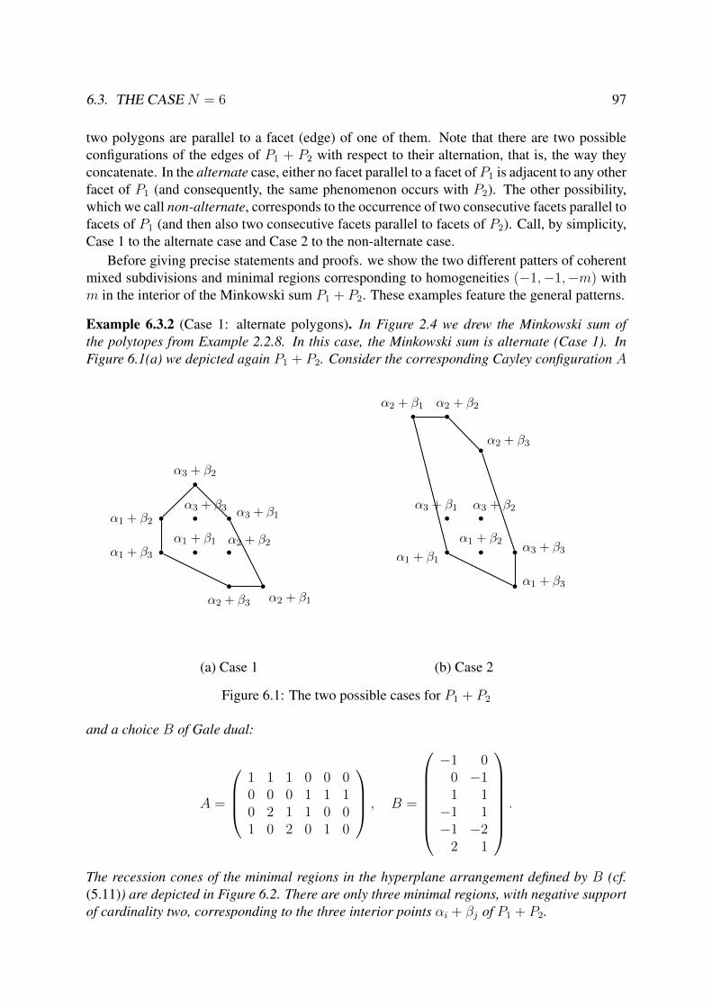
6.3. THE CASE N = 6 97
two polygons are parallel to a facet (edge) of one of them. Note that there are two possibleconfigurations of the edges of P1 + P2 with respect to their alternation, that is, the way theyconcatenate. In the alternate case, either no facet parallel to a facet of P1 is adjacent to any otherfacet of P1 (and consequently, the same phenomenon occurs with P2). The other possibility,which we call non-alternate, corresponds to the occurrence of two consecutive facets parallel tofacets of P1 (and then also two consecutive facets parallel to facets of P2). Call, by simplicity,Case 1 to the alternate case and Case 2 to the non-alternate case.
Before giving precise statements and proofs. we show the two different patters of coherentmixed subdivisions and minimal regions corresponding to homogeneities (−1,−1,−m) withm in the interior of the Minkowski sum P1 + P2. These examples feature the general patterns.
Example 6.3.2 (Case 1: alternate polygons). In Figure 2.4 we drew the Minkowski sum ofthe polytopes from Example 2.2.8. In this case, the Minkowski sum is alternate (Case 1). InFigure 6.1(a) we depicted again P1 + P2. Consider the corresponding Cayley configuration A
bα1 + β3
bα1 + β2
b
α3 + β2
b α3 + β1
b
α2 + β1
b
α2 + β3
b
α2 + β2b
α1 + β1
b
α3 + β3
b
α1 + β1b
α1 + β2
b α1 + β3
b
α2 + β1b
α2 + β2
bα2 + β3
b
α3 + β1b
α3 + β2
b α3 + β3
(a) Case 1 (b) Case 2
Figure 6.1: The two possible cases for P1 + P2
and a choice B of Gale dual:
A =
1 1 1 0 0 00 0 0 1 1 10 2 1 1 0 01 0 2 0 1 0
, B =
−1 0
0 −11 1−1 1−1 −2
2 1
.
The recession cones of the minimal regions in the hyperplane arrangement defined by B (cf.(5.11)) are depicted in Figure 6.2. There are only three minimal regions, with negative supportof cardinality two, corresponding to the three interior points αi + βj of P1 + P2.
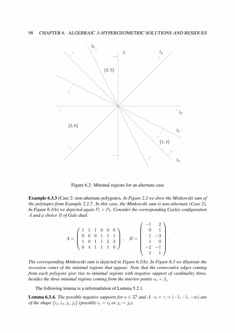
98 CHAPTER 6. ALGEBRAIC A-HYPERGEOMETRIC SOLUTIONS AND RESIDUES
l4
l5
l3
l1
l2
l6
{2, 5}
{1, 4}
{3, 6}
Figure 6.2: Minimal regions for an alternate case
Example 6.3.3 (Case 2: non-alternate polygons). In Figure 2.2 we drew the Minkowski sum ofthe polytopes from Example 2.2.7. In this case, the Minkowski sum is non-alternate (Case 2).In Figure 6.1(b) we depicted again P1 + P2. Consider the corresponding Cayley configurationA and a choice B of Gale dual:
A =
1 1 1 0 0 00 0 0 1 1 11 0 1 1 2 30 4 1 1 1 0
, B =
−1 2
0 11 −31 0−2 −1
1 1
.
The corresponding Minkowski sum is depicted in Figure 6.1(b). In Figure 6.3 we illustrate therecession cones of the minimal regions that appear. Note that the consecutive edges comingfrom each polygons give rise to minimal regions with negative support of cardinality three,besides the three minimal regions coming from the interior points αi + βj .
The following lemma is a reformulation of Lemma 5.2.1.
Lemma 6.3.4. The possible negative supports for u ∈ Z6 and A · u = γ = (−1,−1,−m) areof the shape {i1, i2, j1, j2} (possibly i1 = i2 or j1 = j2).
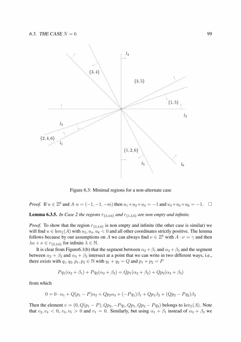
6.3. THE CASE N = 6 99
l3
l5 l6
l4
l2
l1{2, 4, 6}
{1, 5}
{1, 2, 6}
{3, 5}
{3, 4}
Figure 6.3: Minimal regions for a non-alternate case
Proof. If u ∈ Z6 andA·u = (−1,−1,−m) then u1+u2+u3 = −1 and u4+u5+u6 = −1.
Lemma 6.3.5. In Case 2 the regions r{2,4,6} and r{1,2,6} are non empty and infinite.
Proof. To show that the region r{2,4,6} is non empty and infinite (the other case is similar) wewill find u ∈ kerZ(A) with u2, u4, u6 < 0 and all other coordinates strictly positive. The lemmafollows because by our assumptions on A we can always find ν ∈ Z6 with A · ν = γ and thenλu+ ν ∈ r{2,4,6} for infinite λ ∈ N.
It is clear from Figure6.1(b) that the segment between α2 +β1 and α2 +β3 and the segmentbetween α2 + β2 and α3 + β3 intersect at a point that we can write in two different ways, i.e.,there exists with q1, q2, p1, p2 ∈ N with q1 + q2 = Q and p1 + p2 = P
Pq1(α2 + β1) + Pq2(α2 + β3) = Qp1(α2 + β2) +Qp2(α3 + β3)
from which
0 = 0 · α1 +Q(p1 − P )α2 +Qp2α3 + (−Pq1)β1 +Qp1β2 + (Qp2 − Pq2)β3
Then the element v = (0, Q(p1 − P ), Qp2,−Pq1, Qp1, Qp2 − Pq2) belongs to kerZ(A). Notethat v2, v4 < 0, v3, v5 > 0 and v1 = 0. Similarly, but using α1 + β1 instead of α3 + β3 we
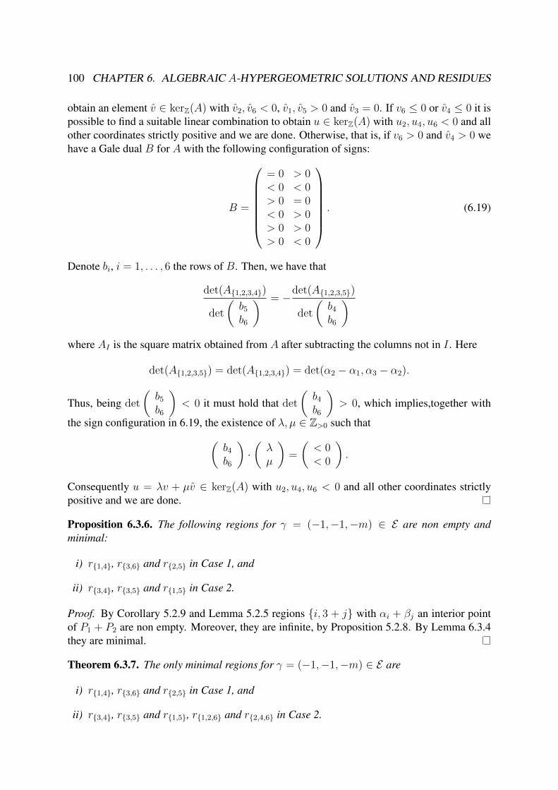
100 CHAPTER 6. ALGEBRAIC A-HYPERGEOMETRIC SOLUTIONS AND RESIDUES
obtain an element v ∈ kerZ(A) with v2, v6 < 0, v1, v5 > 0 and v3 = 0. If v6 ≤ 0 or v4 ≤ 0 it ispossible to find a suitable linear combination to obtain u ∈ kerZ(A) with u2, u4, u6 < 0 and allother coordinates strictly positive and we are done. Otherwise, that is, if v6 > 0 and v4 > 0 wehave a Gale dual B for A with the following configuration of signs:
B =
= 0 > 0< 0 < 0> 0 = 0< 0 > 0> 0 > 0> 0 < 0
. (6.19)
Denote bi, i = 1, . . . , 6 the rows of B. Then, we have that
det(A{1,2,3,4})
det
(b5
b6
) = −det(A{1,2,3,5})
det
(b4
b6
)where AI is the square matrix obtained from A after subtracting the columns not in I . Here
det(A{1,2,3,5}) = det(A{1,2,3,4}) = det(α2 − α1, α3 − α2).
Thus, being det
(b5
b6
)< 0 it must hold that det
(b4
b6
)> 0, which implies,together with
the sign configuration in 6.19, the existence of λ, µ ∈ Z>0 such that(b4
b6
)·(λµ
)=
(< 0< 0
).
Consequently u = λv + µv ∈ kerZ(A) with u2, u4, u6 < 0 and all other coordinates strictlypositive and we are done.
Proposition 6.3.6. The following regions for γ = (−1,−1,−m) ∈ E are non empty andminimal:
i) r{1,4}, r{3,6} and r{2,5} in Case 1, and
ii) r{3,4}, r{3,5} and r{1,5} in Case 2.
Proof. By Corollary 5.2.9 and Lemma 5.2.5 regions {i, 3 + j} with αi + βj an interior pointof P1 + P2 are non empty. Moreover, they are infinite, by Proposition 5.2.8. By Lemma 6.3.4they are minimal.
Theorem 6.3.7. The only minimal regions for γ = (−1,−1,−m) ∈ E are
i) r{1,4}, r{3,6} and r{2,5} in Case 1, and
ii) r{3,4}, r{3,5} and r{1,5}, r{1,2,6} and r{2,4,6} in Case 2.
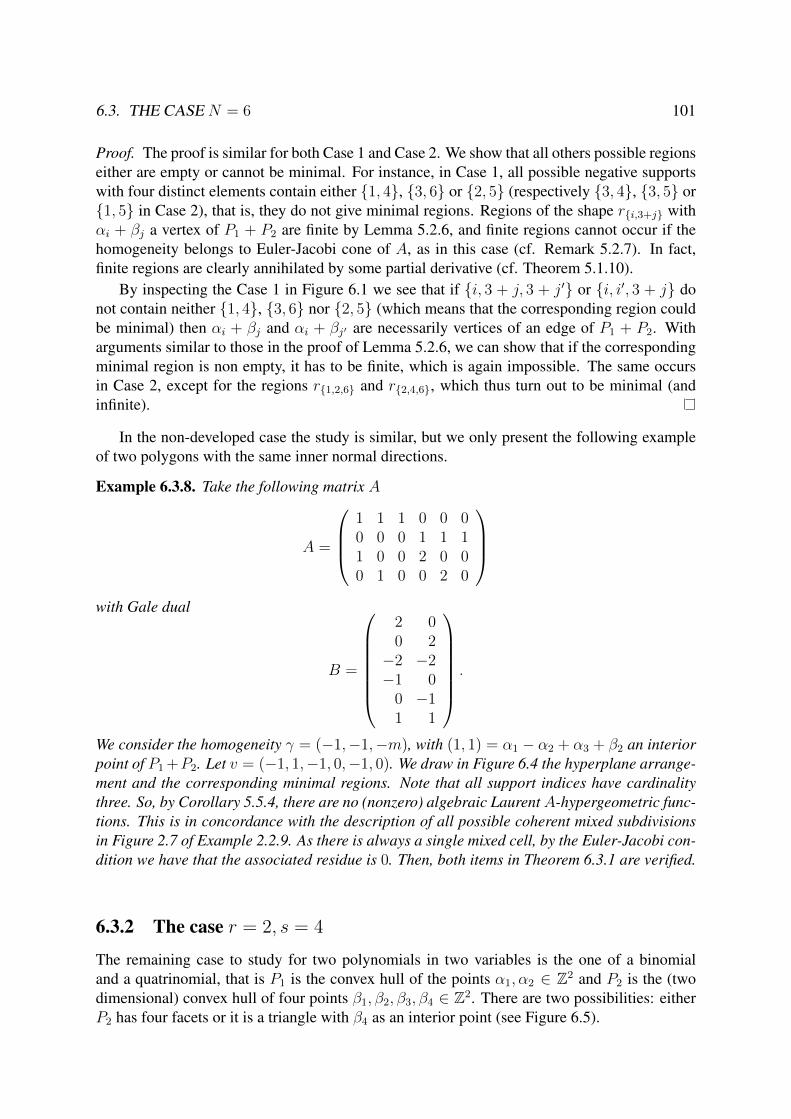
6.3. THE CASE N = 6 101
Proof. The proof is similar for both Case 1 and Case 2. We show that all others possible regionseither are empty or cannot be minimal. For instance, in Case 1, all possible negative supportswith four distinct elements contain either {1, 4}, {3, 6} or {2, 5} (respectively {3, 4}, {3, 5} or{1, 5} in Case 2), that is, they do not give minimal regions. Regions of the shape r{i,3+j} withαi + βj a vertex of P1 + P2 are finite by Lemma 5.2.6, and finite regions cannot occur if thehomogeneity belongs to Euler-Jacobi cone of A, as in this case (cf. Remark 5.2.7). In fact,finite regions are clearly annihilated by some partial derivative (cf. Theorem 5.1.10).
By inspecting the Case 1 in Figure 6.1 we see that if {i, 3 + j, 3 + j′} or {i, i′, 3 + j} donot contain neither {1, 4}, {3, 6} nor {2, 5} (which means that the corresponding region couldbe minimal) then αi + βj and αi + βj′ are necessarily vertices of an edge of P1 + P2. Witharguments similar to those in the proof of Lemma 5.2.6, we can show that if the correspondingminimal region is non empty, it has to be finite, which is again impossible. The same occursin Case 2, except for the regions r{1,2,6} and r{2,4,6}, which thus turn out to be minimal (andinfinite).
In the non-developed case the study is similar, but we only present the following exampleof two polygons with the same inner normal directions.
Example 6.3.8. Take the following matrix A
A =
1 1 1 0 0 00 0 0 1 1 11 0 0 2 0 00 1 0 0 2 0
with Gale dual
B =
2 00 2−2 −2−1 0
0 −11 1
.
We consider the homogeneity γ = (−1,−1,−m), with (1, 1) = α1 − α2 + α3 + β2 an interiorpoint of P1 +P2. Let v = (−1, 1,−1, 0,−1, 0). We draw in Figure 6.4 the hyperplane arrange-ment and the corresponding minimal regions. Note that all support indices have cardinalitythree. So, by Corollary 5.5.4, there are no (nonzero) algebraic LaurentA-hypergeometric func-tions. This is in concordance with the description of all possible coherent mixed subdivisionsin Figure 2.7 of Example 2.2.9. As there is always a single mixed cell, by the Euler-Jacobi con-dition we have that the associated residue is 0. Then, both items in Theorem 6.3.1 are verified.
6.3.2 The case r = 2, s = 4
The remaining case to study for two polynomials in two variables is the one of a binomialand a quatrinomial, that is P1 is the convex hull of the points α1, α2 ∈ Z2 and P2 is the (twodimensional) convex hull of four points β1, β2, β3, β4 ∈ Z2. There are two possibilities: eitherP2 has four facets or it is a triangle with β4 as an interior point (see Figure 6.5).
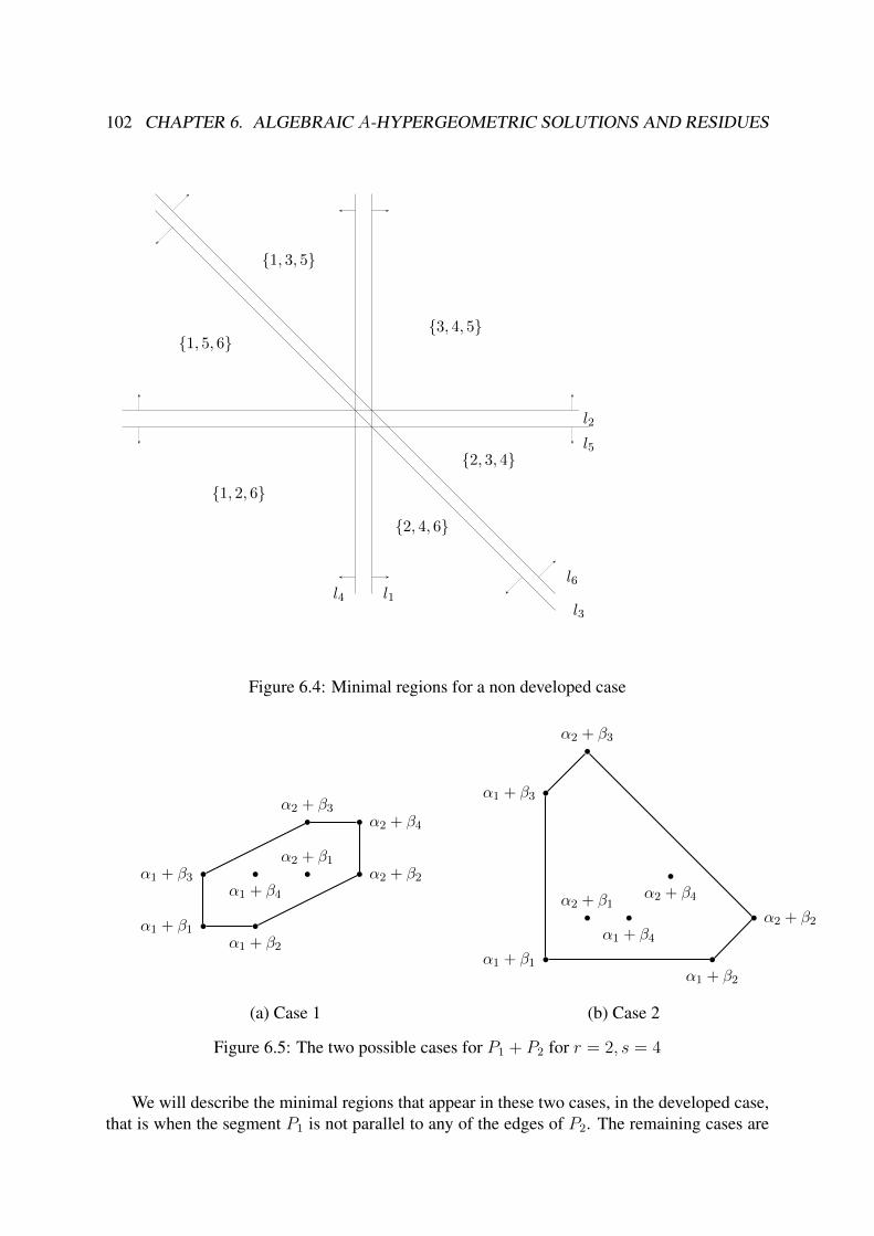
102 CHAPTER 6. ALGEBRAIC A-HYPERGEOMETRIC SOLUTIONS AND RESIDUES
l1
l2
l3l4
l5
l6
{3, 4, 5}
{1, 3, 5}
{1, 5, 6}
{1, 2, 6}
{2, 4, 6}
{2, 3, 4}
Figure 6.4: Minimal regions for a non developed case
bα1 + β1 b
α1 + β2
bα1 + β3 b
α1 + β4
b
α2 + β1b α2 + β2
b
α2 + β3b α2 + β4
bα1 + β1 b
α1 + β2
bα1 + β3
b
α1 + β4
b
α2 + β1b α2 + β2
b
α2 + β3
b
α2 + β4
(a) Case 1 (b) Case 2
Figure 6.5: The two possible cases for P1 + P2 for r = 2, s = 4
We will describe the minimal regions that appear in these two cases, in the developed case,that is when the segment P1 is not parallel to any of the edges of P2. The remaining cases are
6.4. GENERAL CONJECTURES 103
also straightforward. We proceed in a similar fashion than in the the case r = s = 3. Note thatLemma 6.3.4 holds in the case as well, since it only depends on the fact that γ1 = γ2 = −1 arenegative.
Lemma 6.3.9. The regions r{1,4,5} and r{2,4,5} in Case 1 and the region r{1,4,5} in Case 2 arenon empty and infinite.
Proof. For the region r{1,4,5} in Case 1, take q1, q2, p1, p2 ∈ N with q1+q2 = Q and p1+p2 = Pto write
Pq1(α1 + β2) + Pq2(α1 + β3) = Qp1(α1 + β1) +Qp2(α2 + β4).
Then, the vector (Q(p1 − P ), Qp2, Qp1,−Pq1,−Pq2, Qp2) ∈ kerZ(A). For the region r{2,4,5}in Case 1 proceed similarly.
For the region r{1,4,5} in Case 2 we can proceed in a similar fashion as in Lemma 6.3.5.
Finally, we can argue as in the case r = s = 3 to give a complete picture of the minimalregions in this case. We have the following analog results and similar conclusions than in theprevious case.
Proposition 6.3.10. Let m ∈ (P1 + P2)◦ then the only minimal regions for γ = (−1,−1,−m)are
i) r{1,6}, r{2,3}, r{1,4,5} and r{2,4,5} in the Case 1 and
ii) r{1,6}, r{2,6}, r{2,3} and r{1,4,5} in the Case 2.
In Case 1, the six different mixed coherent subdivisions Πw, depicted in Figure 2.9, havetwo possible different shapes. Either there is one interior vertex (α1 + β4 = α2 + β1) and twomixed cells σ1, σ2 which contain it, or there is a single mixed cell and the only minimal regionsin the direction ofw have negative support r{1,4,5} and r{2,4,5}, which cannot give rise to Laurentalgebraic solutions. Thus, we check the validity of the facts in the proof of Theorem 6.3.1. InCase 2, however, the situation is not covered exactly by this result and we detail it in the nextsection.
6.4 General conjectures
We end this chapter with natural general conjectures for future work. We expect that undervery general conditions, Conjecture 6.4.3 below holds true.
Note that for configurations with interior points, there might be vertices of coherent mixedsubdivisions which need not be vertices of a mixed cell. Our next example shows this behaviourand some new associated features.
Example 6.4.1. Let A be as in Example 2.2.11, corresponding to a configuration termed asCase 2 at the end of the previous section. Note that the two interior points (1, 1) = α1 + β4 =α2 + β1 and (2, 2) = α2 + β4 of A1 + A2 show the following “new” behaviour:
• Both occur as vertices of a coherent mixed subdivision, but not as vertices of a mixed cellof this subdivision.

104 CHAPTER 6. ALGEBRAIC A-HYPERGEOMETRIC SOLUTIONS AND RESIDUES
• The point (2, 2) never occurs as a vertex of a mixed cell without (1, 1) being another suchvertex. They “share” the same mixed cells.
Let γ = (−1,−1,−1,−1). The corresponding central arrangement is depicted in Figure 6.6,using the Gale dual configuration given by {(−1, 1), (0, 1), (0, 1), (1,−3), (1, 0), (−1, 0)}.
l3l1l2
l4 = l5
l6
{2, 3}
{2, 6}
{1, 6}
{1, 4, 5}
Figure 6.6: Minimal regions for Example 6.4.1
There are three minimal regions with negative support of cardinality three (one correspond-ing to (2, 2) and the two others corresponding to the two expressions for (1, 1).) Let w withbw :=
∑6i=1wibi lying in the positive cone spanned by b1 and b4, b5. We see that the point (2, 2)
is a vertex of Πw which is not in a mixed cell. The corresponding region (with minimal supportI = {2, 6}) gives rise to a non-algebraic canonical Laurent series ΦI . This can be seen byrestricting ΦI to the vertical boundary ray.
The canonical series ΦJ , J = {2, 3} corresponding to the decomposition (1, 1) = α2 + β2
is algebraic since this point is a vertex of a mixed cell in Πw, for any w with bw in the positivecone spanned by b6 and b4, b5. On the other side, the canonical series ΦK , K = {1, 6},corresponding to the decomposition (1, 1) = α1 +β4 is again not algebraic (seen by restrictionto its vertical boundary ray). In this case the point does not occur as a vertex of a mixed cell(but it is a vertex of Piw for any bw in the positive cone spanned by b2 and b3.).
Indeed, let any w with bw in the positive cone spanned by b3 and b4, b5. The correspondingcoherent mixed decomposition has two mixed cells σ1, σ2 and the dimension of the space of
6.4. GENERAL CONJECTURES 105
residues is one. However, there are two interior vertices (2, 2) and (1, 1) = α1 + β4; choosingm equal to any of them, Theorem 6.2.2 gives us the decomposition
Resmσi = ΦK − ΦJ .
Thus, the linear combination ΦK−ΦJ is algebraic and the dimension of the space of algebraicA-hypergeometric functions in the direction of w is one, that is, it is equal to the number ofmixed cells minus one, but it does not equal the number of interior vertices of these cells, whichis two.
We now state our first conjecture:
Conjecture 6.4.2. Let w ∈ Rn generic and v = αi + βj ∈ Πw an interior point of P1 + P2
which does not belong to any mixed cell. Then the canonical Laurent series with negativesupport {i, j} is not algebraic. Here it is assumed that if v can also be written as α` +αk, withi 6= `, j 6= k then wi + wj < w` + wk.
We now state our main conjecture:
Conjecture 6.4.3. Let w be a generic weight in Rn, and A1, A2 two general planar configura-tions. Then, for any γ = (−1,−1,−m) with m ∈ (A1 + A2)◦ ∩ Z2,
Algγ,w = Rγ,w (6.20)
It would be interesting to find combinatorial conditions that ensure that all canonical seriesΦij := Φγ
r{i,j}corresponding to interior vertices of Πw which lie in mixed cells, can be written
in terms of residues. We would need to invert the explicit expressions given in Theorem 6.2.2:
Resmσ (x) =∑
kσ,vΦγr{i,j}
(x).
This seems to be easy in the case all the points of the configurations are vertices but ratherdifficult in general. The understanding of this question would lead to an explicit combinatorialformula for the dimension of Algγ,w.

106 CHAPTER 6. ALGEBRAIC A-HYPERGEOMETRIC SOLUTIONS AND RESIDUES

Bibliography
[ACG96] A. Assi, F. J. Castro-Jimenez, and J. M. Granger. How to calculate the slopes of aD-module. Compositio Math., 104(2):107–123, 1996.
[ACG00] A. Assi, F. J. Castro-Jimenez, and M. Granger. The Grobner fan of an An-module.J. Pure Appl. Algebra, 150(1):27–39, 2000.
[Ado94] A. Adolphson. Hypergeometric functions and rings generated by monomials. DukeMath. J., 73(2):269–290, 1994.
[Ber10] C. Berkesch. Euler–Koszul methods in algebra and geometry. PhD thesis, PurdueUniversity, 2010.
[Beu10] F. Beukers. Algebraic A-hypergeometric functions. Invent. Math., 180:589–610,2010.
[BH89] F. Beukers and G. Heckman. Monodromy for the hypergeometric function nFn−1.Invent. Math., 95(2):325–354, 1989.
[CDD99] E. Cattani, C. D’Andrea, and A. Dickenstein. The a-hypergeometric system asso-ciated with a monomial curve. Duke Math. J., 99(2):179–207, 1999.
[CDR11] E. Cattani, A. Dickenstein, and F. Rodrıguez Villegas. The structure of bivariaterational hypergeometric functions. International Mathematics Research Notices,2011:2496–2533, 2011.
[CDS01] E. Cattani, A. Dickenstein, and Bernd Sturmfels. Rational hypergeometric func-tions. Compositio Math., 128(2):217–239, 2001.
[CF11] F. J. Castro–Jimenez and M. C. Fernandez–Fernandez. Gevrey solutions forirregular hypergeometric systems I. Transactions of the Amer. Math. Society,363(2):923–948, 2011.
[CL55] E.A. Coddington and N. Levinson. Theory of ordinary differential equations.McGraw-Hill Book Company, Inc., New York-Toronto-London, 1955.
[Cop34] F. T. Cope. Formal Solutions of Irregular Linear Differential Equations. Part I.Amer. J. Math., 56(1-4):411–437, 1934.
[CT03] F. J. Castro-Jimenez and N. Takayama. Singularities of the hypergeometric systemassociated with a monomial curve. Trans. Amer. Math. Soc., 355(9):3761–3775(electronic), 2003.
107
108 BIBLIOGRAPHY
[Dic04] A. Dickenstein. Hypergeometric functions with integer homogeneities. InGeometrie Complexe II, Eds. F.Norguet- S. Ofman, ”Actualites scientifiques et in-dustrielles”, Ed. Hermann, 2004. 2004.
[DRS10] J. De Loera, J. A. Rambau, and F. Santos. Triangulations, volume 25 of Algorithmsand Computation in Mathematics. Springer-Verlag, Berlin, 2010. Structures foralgorithms and applications.
[Fer10] M. C. Fernandez–Fernandez. Irregular hypergeometric D-modules. Adv. Math.,224(5):1735–1764, 2010.
[GK96] O.A. Gel′fond and A.G. Khovanskii. Newtonian polyopes and grotendieckresidues. Dokl. Math., 54:700–702, 1996.
[GKZ88] I. M. Gel′fand, M. M. Kapranov, and A. V. Zelevinsky. Equations of hypergeomet-ric type and newton polyhedra. Dokl. Akad. Nauk SSSR, 300(3):529–534, 1988.
[GKZ89] I. M. Gel′fand, M. M. Kapranov, and A. V. Zelevinsky. Hypergeometric functionsand toric varieties. Funktsional. Anal. i Prilozhen., 23(2):12–26, 1989.
[GKZ90] I. M. Gel′fand, M. M. Kapranov, and A. V. Zelevinsky. Generalized euler integralsand a-hypergeometric functions. Adv. Math., 84(2):255–271, 1990.
[GKZ94] I. M. Gel′fand, M. M. Kapranov, and A. V. Zelevinsky. Discriminants, resul-tants, and multidimensional determinants. Mathematics: Theory & Applications.Birkhauser Boston Inc., Boston, MA, 1994.
[Har03] M. I. Hartillo Hermoso. Slopes of hypergeometric systems of codimension one.In Proceedings of the International Conference on Algebraic Geometry and Singu-larities (Spanish) (Sevilla, 2001), volume 19, pages 455–466, 2003.
[Har05] M. I. Hartillo-Hermoso. Irregular hypergeometric systems associated with a sin-gular monomial curve. Trans. Amer. Math. Soc., 357(11):4633–4646 (electronic),2005.
[Hot91] R. Hotta. Equivariant D-modules. In Proceedings of ICPAM Spring School inWuhan, 1991.
[HS95] B. Huber and B. Sturmfels. A polyhedral method for solving sparse polynomialsystems. Mathematics of Computation, 64(212):1541–1555, 1995.
[Kho78] A. G. Khovanskii. Newton polyhedra and the euler-jacobi formula. Russian Math.Surveys, 33:237–238, 1978.
[Lau87] Yves Laurent. Polygone de Newton et b-fonctions pour les modules microd-ifferentiels. Ann. Sci. Ecole Norm. Sup. (4), 20(3):391–441, 1987.
[LM99] Y. Laurent and Z. Mebkhout. Pentes algebriques et pentes analytiques d’un D-module. Ann. Sci. Ecole Norm. Sup. (4), 32(1):39–69, 1999.

BIBLIOGRAPHY 109
[May37] K. Mayr. Uber die Losung algebraischer Gleichungssysteme durch hyperge-ometrische Funktionen. Monatsh Math. Phys., 45:280–313, 1937.
[Meb89] Z. Mebkhout. Le theoreme de comparaison entre cohomologies de de Rham d’unevariete algebrique complexe et le theoreme d’existence de Riemann. Inst. HautesEtudes Sci. Publ. Math., (69):47–89, 1989.
[MMW05] L. F. Matusevich, E. Miller, and U. Walther. Homological methods for hypergeo-metric families. J. Amer. Math. Soc., 18(4):919–941 (electronic), 2005.
[MR88] T. Mora and L. Robbiano. The Grobner fan of an ideal. J. Symbolic Comput.,6(2-3):183–208, 1988. Computational aspects of commutative algebra.
[OT09] K. Ohara and N. Takayama. Holonomic rank of A -hypergeometric differential-difference equations. J. Pure Appl. Algebra, 213(8):1536–1544, 2009.
[PST05] M. Passare, T. Sadykov, and A. Tsikh. Singularities of hypergeometric functionsin several variables. Compositio Matth, 141(3):787–810, 2005.
[Rod] F. Rodrıguez Villegas. Integral ratios of factorials and algebraic hypergeometricfunctions. arXiv:math.NT/0701362.
[Sai02] M. Saito. Logarithm-free A-hypergeometric series. Duke Math. J., 115(1):53–73,2002.
[SST00] M. Saito, B. Sturmfels, and N. Takayama. Grobner deformations of hypergeomet-ric differential equations, volume 6 of Algorithms and Computation in Mathemat-ics. Springer-Verlag, Berlin, 2000.
[Stu96] B. Sturmfels. Grobner bases and convex polytopes, volume 8 of University LectureSeries. American Mathematical Society, Providence, RI, 1996.
[Stu00] B. Sturmfels. Solving algebraic equations in terms of A-hypergeometric series.Discrete Math., 210(1–3):171–181, 2000.
[STV95] B. Sturmfels, N. V. Trung, and W. Vogel. Bounds on degrees of projective schemes.Math. Ann., 302(3):417–432, 1995.
[SW08] M. Schulze and U. Walther. Irregularity of hypergeometric systems via slopesalong coordinate subspaces. Duke Math. J., 142(3):465–509, 2008.