Sesión 009. “Del cerebro al mercado: Redes Neuronales”1480-Técnicas Estadísticas en Investigación de MercadosGrado en Estadística EmpresarialProfesor: Xavier Barber i VallésDepartamento: Estadística, Matemáticas e Informática

REDES NEURONALES APLICADAS AL MARKETING

Índice

• Definición• Aplicaciones al Marketing• La Neurona• RNA como modelos predictivos

¿Redes Neuronales?• Finanzas:

– Asignación de Recursos, – Scheduling, ...

• Marketing:– Planificación de eventos,– Clasificación de Clientes,..

• Ciencias de la Salud:……

Las Redes Neuronales han pasado a ser una buena Herramienta para comprender y poder predecir un complejo

sistema de variables que están interrelacionadas.

• Biología– Aprender más acerca del cerebro y otros sistemas.– Obtención de modelos de la retina.

• Empresas– Evaluación de probabilidad de formaciones geológicas y petrolíferas.– Identificación de candidatos para posiciones específicas.– Explotación de Bases de Datos.– Optimización de plazas y horarios en líneas de vuelo.– Reconocimiento de caracteres escritos.

• Medio Ambiente– Analizar tendencias y patrones.– Previsión del Tiempo.

• Finanzas– Previsión de la evolución de los precios.– Valoración del Riesgo de los créditos.– Identificación de falsificaciones.– Interpretación de firmas.

• Manufacturación– Robots automatizados y sistemas de control (visión artificial y sensores de presión, temperatura, gas, etc.)– Control de producción en líneas de proceso.– Inspección de la calidad.

• Medicina– Analizadores del habla para la ayuda en la audición en sordos profundos.– Diagnóstico y tratamiento a partir de síntomas y/o de datos analíticos (electrocardiograma, encefalograma, análisis sanguíneo, etc.)– Monitorización en cirugía.– Predicción de reacciones adversas a los medicamentos.– Lectores de Rayos X.– Entendimiento de la causa de los ataques epilépticos.

• Militares– Clasificación de las señales de radar.– Creación de Armas Inteligentes.– Optimización del uso de recursos escasos.– Reconocimiento y seguimiento en el tiro al blanco.

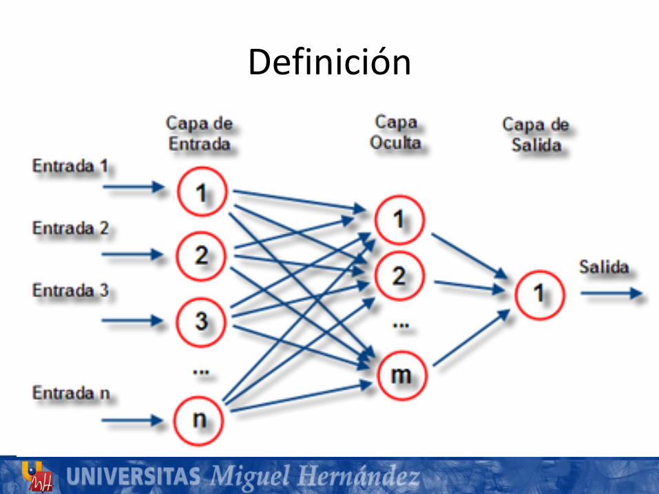
DefiniciónLas Redes Neuronales (ANN: Artificial Neural Networks)surgieron originalmente como una simulación abstracta de lossistemas nerviosos biológicos, constituidos por un conjunto deunidades llamadas neuronas conectadas unas conotras.

El primer modelo de red neuronal fue propuesto en 1943 porMcCulloch y Pitts en términos de un modelo computacionalde actividad nerviosa. Este modelo era un modelo binario,donde cada neurona tenía un escalón o umbral prefijado, ysirvió de base para los modelos posteriores.

Aplicaciones en Marketing

• Segmentación y Detección del público objetivo (Target).

• Investigación y modelización del comportamiento del consumidor.

• Previsión de Ventas.• Modelos de determinación de Precios.• Combinación de Procesos en distribución comercial.• Toma de decisiones en marketing (lanzamientos de

productos, etc.).• Modelos de respuestas publicitaria.

Aplicaciones en Marketing

Si bien la gran mayoría de epígrafes anteriores tenemos técnicas ya muy contrastadas para resolverlas…

¿qué me aportan la Redes Neuronales?

No necesito LinealidadNo necesito cumplimiento de hipótesis iniciales…

¡¡¡Pero no lo resuelven todo Siempre!!!

La Neurona

http://teembo.com/jagr/Articulo_Tecnico_Redes_Neuronales_Reconocimiento_Patrones.php

http://www.monografias.com/trabajos/redesneuro/redesneuro.shtml

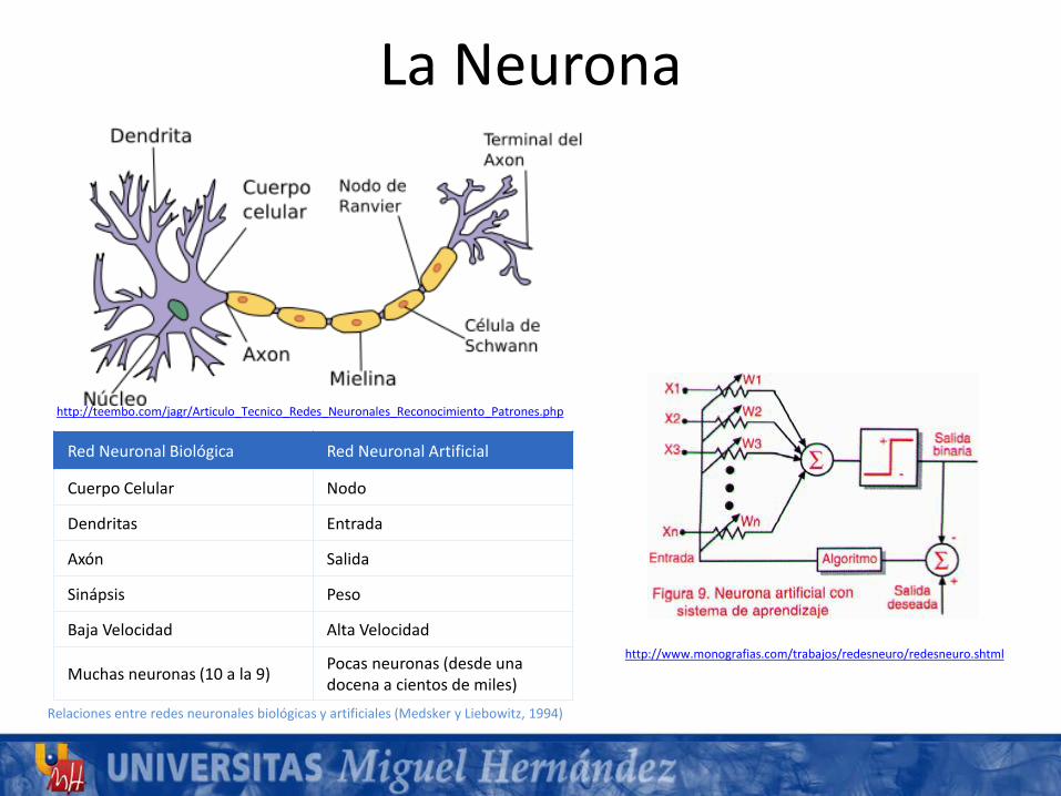
Red Neuronal Biológica Red Neuronal Artificial

Cuerpo Celular Nodo

Dendritas Entrada

Axón Salida

Sinápsis Peso

Baja Velocidad Alta Velocidad

Muchas neuronas (10 a la 9) Pocas neuronas (desde una docena a cientos de miles)

Relaciones entre redes neuronales biológicas y artificiales (Medsker y Liebowitz, 1994)

RNA como modelos predictivos

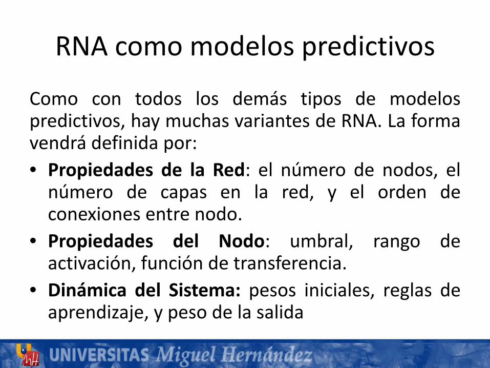
Como con todos los demás tipos de modelospredictivos, hay muchas variantes de RNA. La formavendrá definida por:• Propiedades de la Red: el número de nodos, el

número de capas en la red, y el orden deconexiones entre nodo.

• Propiedades del Nodo: umbral, rango deactivación, función de transferencia.

• Dinámica del Sistema: pesos iniciales, reglas deaprendizaje, y peso de la salida

RNA como modelos predictivos

Estas propiedades están todas implementadascomo relaciones matemáticas entre inputs youtputs.• Bishop, C.M. (1995) Neural Networks for Pattern Recognition, Oxford:

Oxford University Press. ISBN 0-19-853849-9.

• Ripley, Brian D. (1996) Pattern Recognition and Neural Networks, Cambridge.

• Sergios Theodoridis, Konstantinos Koutroumbas (2009) "PatternRecognition", 4th Edition, Academic Press, ISBN 978-1-59749-272-0.

RNA como modelos predictivos

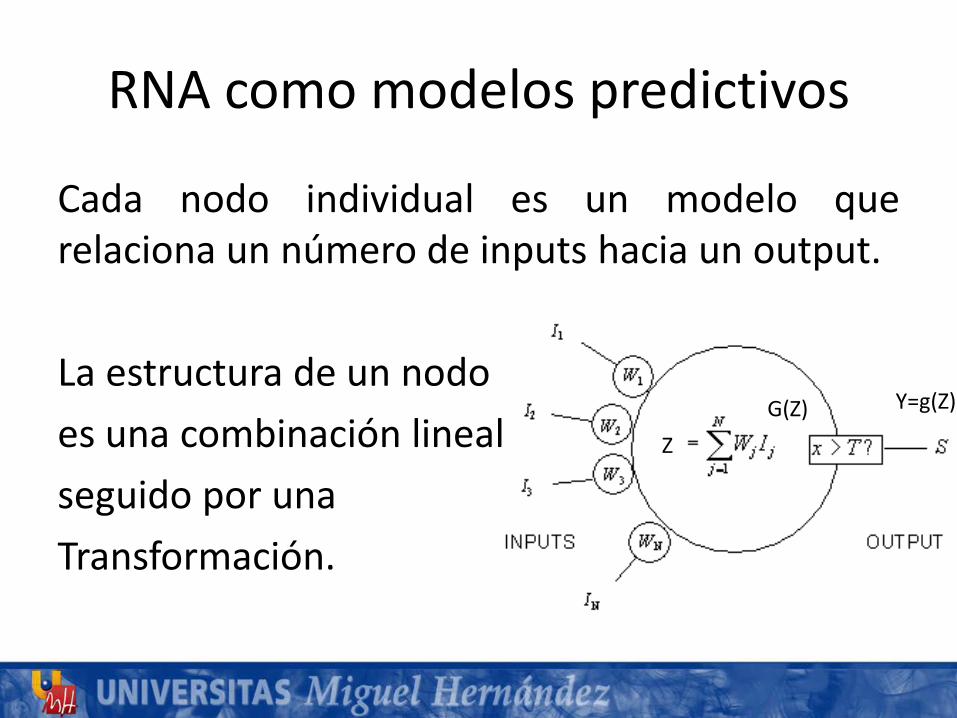
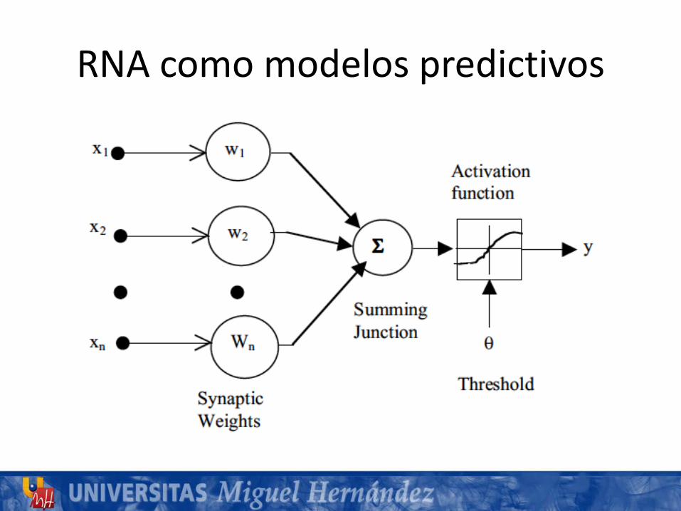
Cada nodo individual es un modelo querelaciona un número de inputs hacia un output.

La estructura de un nodoes una combinación linealseguido por unaTransformación.

ZG(Z) Y=g(Z)

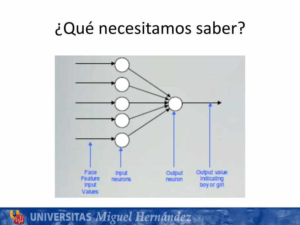
¿Qué necesitamos saber?

RNA como modelos predictivos

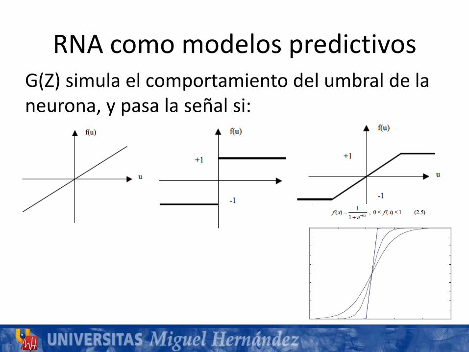
RNA como modelos predictivosG(Z) simula el comportamiento del umbral de la neurona, y pasa la señal si:

RNA como modelos predictivos

Creamos la RED al conectar unos nodos con otros, ytenemos una arquitectura escrita de formamatemática.

Vamos sustituyendo los outputs por los resultadosobtenidos en otros nodos….

Las RNA tienen un buen comportamiento sobre eloverfitting, y suelen generar modelos pequeños.

RNA como modelos predictivos

Resumiendo:• Las RNA pueden aprender a representar unos

datos , con algún tipo de relación funcional entrelas variables, para adquiere un grado de ajustecon un número suficiente de nodos y capasocultas.

• Esto nos permite capturar relaciones ocultas sinnecesidad de buscar esa estructura.

• Y no necesitamos conocer el funcionamiento denuestro problema, sólo hay que “entrenarlo”suficientemente.

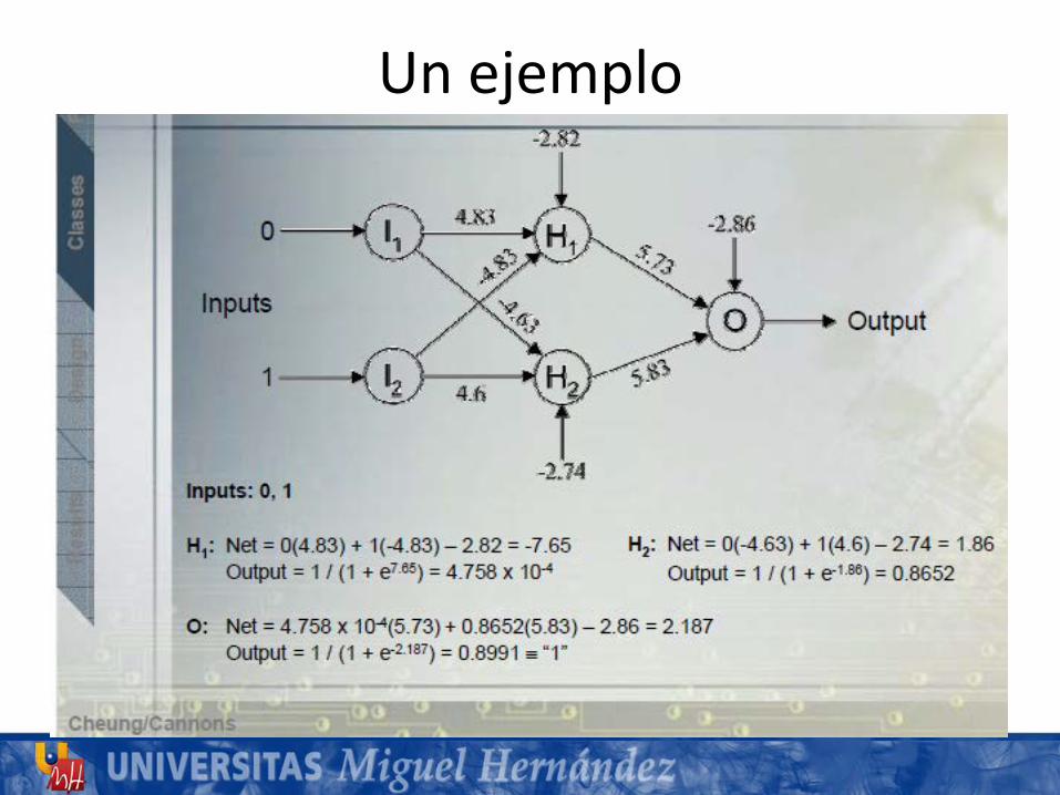
Un ejemplo

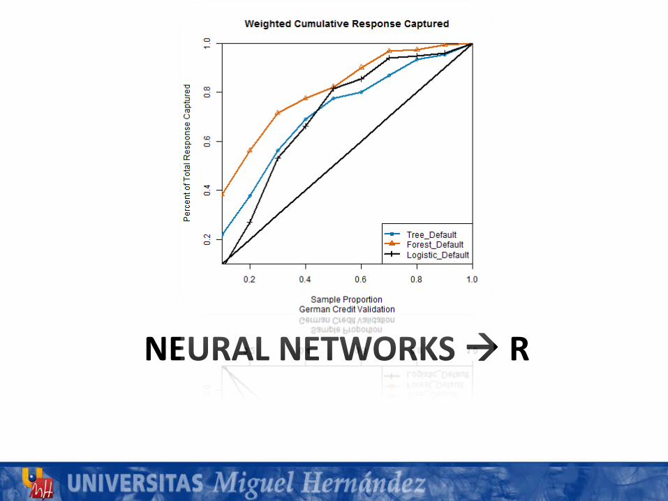
NEURAL NETWORKS R

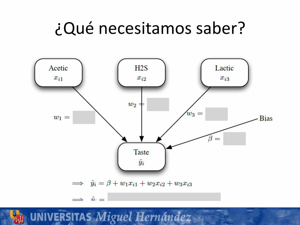
¿Qué necesitamos saber?

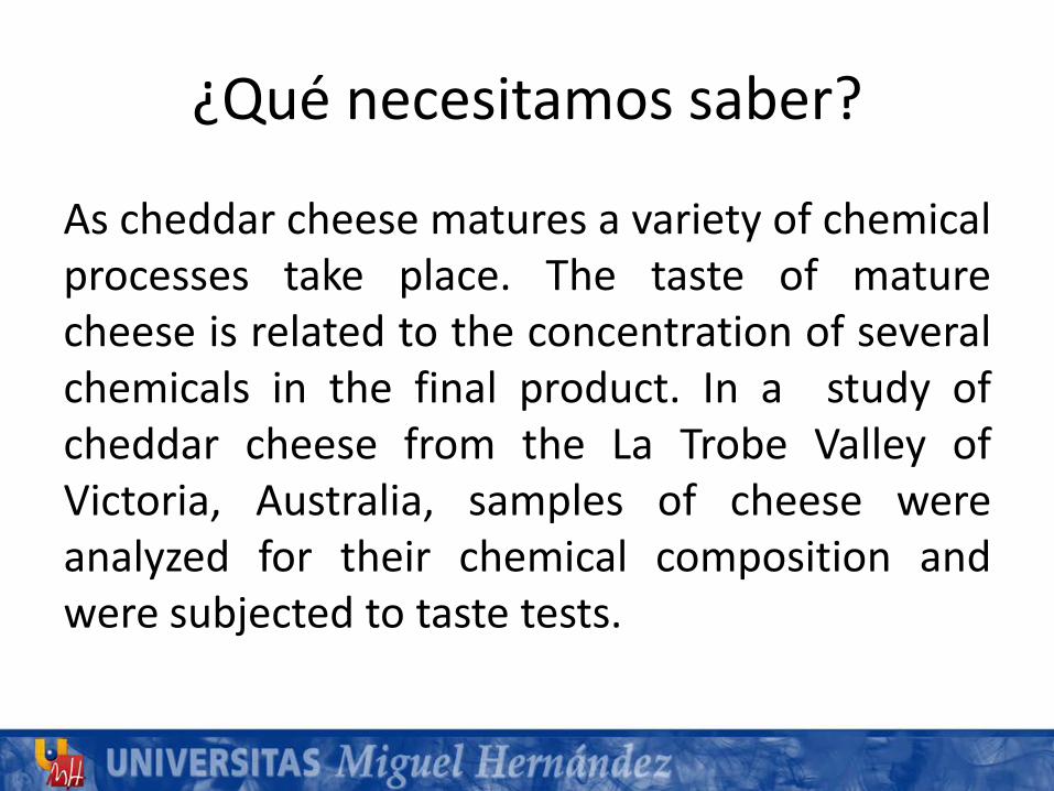
As cheddar cheese matures a variety of chemicalprocesses take place. The taste of maturecheese is related to the concentration of severalchemicals in the final product. In a study ofcheddar cheese from the La Trobe Valley ofVictoria, Australia, samples of cheese wereanalyzed for their chemical composition andwere subjected to taste tests.

¿Qué necesitamos saber?

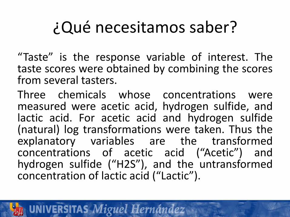
“Taste” is the response variable of interest. Thetaste scores were obtained by combining the scoresfrom several tasters.Three chemicals whose concentrations weremeasured were acetic acid, hydrogen sulfide, andlactic acid. For acetic acid and hydrogen sulfide(natural) log transformations were taken. Thus theexplanatory variables are the transformedconcentrations of acetic acid (“Acetic”) andhydrogen sulfide (“H2S”), and the untransformedconcentration of lactic acid (“Lactic”).

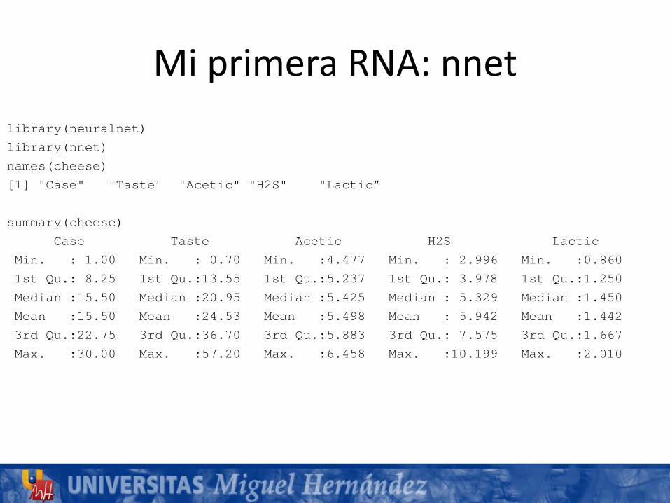
Mi primera RNA: nnetlibrary(neuralnet)

library(nnet)

names(cheese)

[1] "Case" "Taste" "Acetic" "H2S" "Lactic”

summary(cheese)

Case Taste Acetic H2S Lactic

Min. : 1.00 Min. : 0.70 Min. :4.477 Min. : 2.996 Min. :0.860

1st Qu.: 8.25 1st Qu.:13.55 1st Qu.:5.237 1st Qu.: 3.978 1st Qu.:1.250

Median :15.50 Median :20.95 Median :5.425 Median : 5.329 Median :1.450

Mean :15.50 Mean :24.53 Mean :5.498 Mean : 5.942 Mean :1.442

3rd Qu.:22.75 3rd Qu.:36.70 3rd Qu.:5.883 3rd Qu.: 7.575 3rd Qu.:1.667

Max. :30.00 Max. :57.20 Max. :6.458 Max. :10.199 Max. :2.010

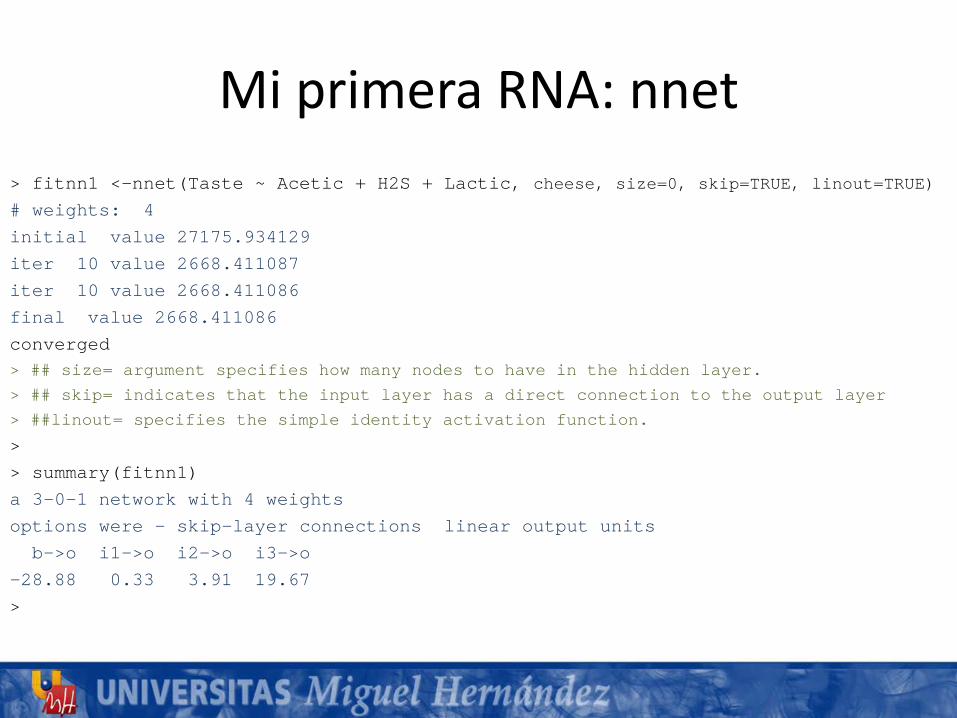
Mi primera RNA: nnet> fitnn1 <-nnet(Taste ~ Acetic + H2S + Lactic, cheese, size=0, skip=TRUE, linout=TRUE)

# weights: 4

initial value 27175.934129

iter 10 value 2668.411087

iter 10 value 2668.411086

final value 2668.411086

converged> ## size= argument specifies how many nodes to have in the hidden layer.

> ## skip= indicates that the input layer has a direct connection to the output layer

> ##linout= specifies the simple identity activation function.

>

> summary(fitnn1)

a 3-0-1 network with 4 weights

options were - skip-layer connections linear output units

b->o i1->o i2->o i3->o

-28.88 0.33 3.91 19.67

>

¿Qué necesitamos saber?

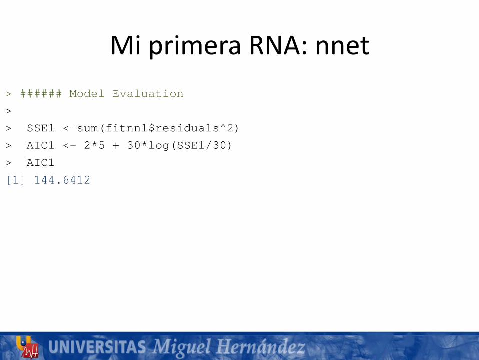
Mi primera RNA: nnet> ###### Model Evaluation

>

> SSE1 <-sum(fitnn1$residuals^2)

> AIC1 <- 2*5 + 30*log(SSE1/30)

> AIC1

[1] 144.6412

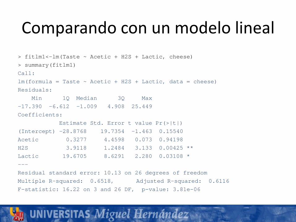
Comparando con un modelo lineal> fitlm1<-lm(Taste ~ Acetic + H2S + Lactic, cheese)

> summary(fitlm1)

Call:

lm(formula = Taste ~ Acetic + H2S + Lactic, data = cheese)

Residuals:

Min 1Q Median 3Q Max

-17.390 -6.612 -1.009 4.908 25.449

Coefficients:

Estimate Std. Error t value Pr(>|t|)

(Intercept) -28.8768 19.7354 -1.463 0.15540

Acetic 0.3277 4.4598 0.073 0.94198

H2S 3.9118 1.2484 3.133 0.00425 **

Lactic 19.6705 8.6291 2.280 0.03108 *

---

Residual standard error: 10.13 on 26 degrees of freedom

Multiple R-squared: 0.6518, Adjusted R-squared: 0.6116

F-statistic: 16.22 on 3 and 26 DF, p-value: 3.81e-06

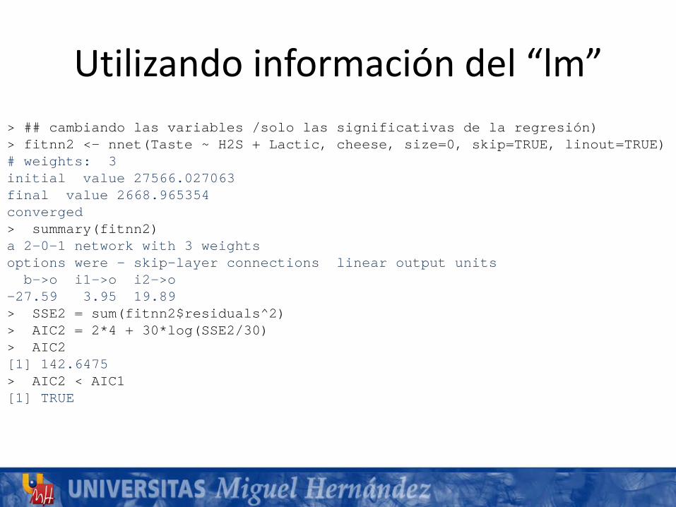
Utilizando información del “lm”> ## cambiando las variables /solo las significativas de la regresión)> fitnn2 <- nnet(Taste ~ H2S + Lactic, cheese, size=0, skip=TRUE, linout=TRUE)# weights: 3initial value 27566.027063 final value 2668.965354 converged> summary(fitnn2)a 2-0-1 network with 3 weightsoptions were - skip-layer connections linear output units

b->o i1->o i2->o -27.59 3.95 19.89 > SSE2 = sum(fitnn2$residuals^2)> AIC2 = 2*4 + 30*log(SSE2/30)> AIC2[1] 142.6475> AIC2 < AIC1[1] TRUE

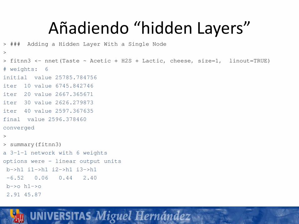
Añadiendo “hidden Layers”> ### Adding a Hidden Layer With a Single Node

>

> fitnn3 <- nnet(Taste ~ Acetic + H2S + Lactic, cheese, size=1, linout=TRUE)

# weights: 6

initial value 25785.784756

iter 10 value 6745.842746

iter 20 value 2667.365671

iter 30 value 2626.279873

iter 40 value 2597.367635

final value 2596.378460

converged

>

> summary(fitnn3)

a 3-1-1 network with 6 weights

options were - linear output units

b->h1 i1->h1 i2->h1 i3->h1

-6.52 0.06 0.44 2.40

b->o h1->o

2.91 45.87

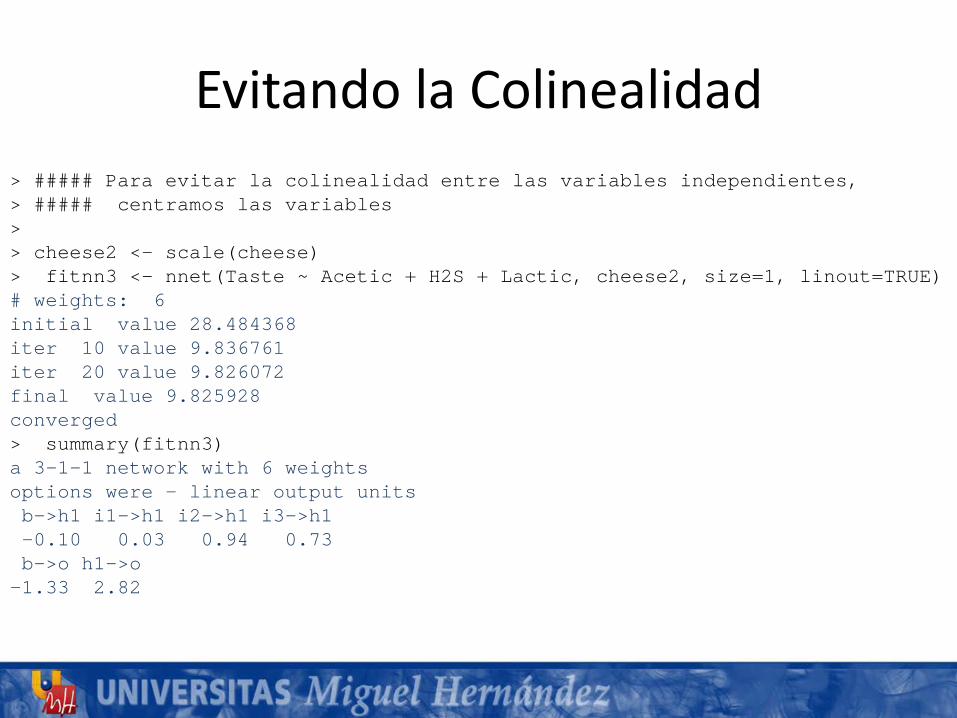
Evitando la Colinealidad> ##### Para evitar la colinealidad entre las variables independientes,> ##### centramos las variables> > cheese2 <- scale(cheese)> fitnn3 <- nnet(Taste ~ Acetic + H2S + Lactic, cheese2, size=1, linout=TRUE)# weights: 6initial value 28.484368 iter 10 value 9.836761iter 20 value 9.826072final value 9.825928 converged> summary(fitnn3)a 3-1-1 network with 6 weightsoptions were - linear output unitsb->h1 i1->h1 i2->h1 i3->h1 -0.10 0.03 0.94 0.73 b->o h1->o -1.33 2.82

RNA como herramientasde Clasificación

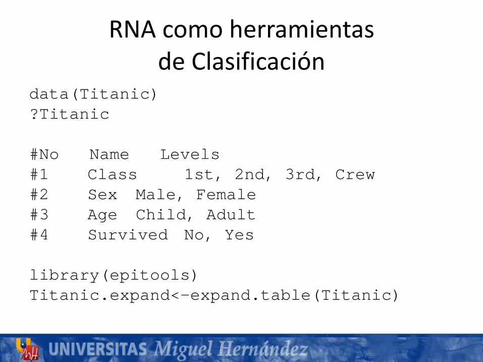
data(Titanic)?Titanic

#No Name Levels#1 Class 1st, 2nd, 3rd, Crew#2 Sex Male, Female#3 Age Child, Adult#4 Survived No, Yes

library(epitools)Titanic.expand<-expand.table(Titanic)

RNA como herramientasde Clasificación

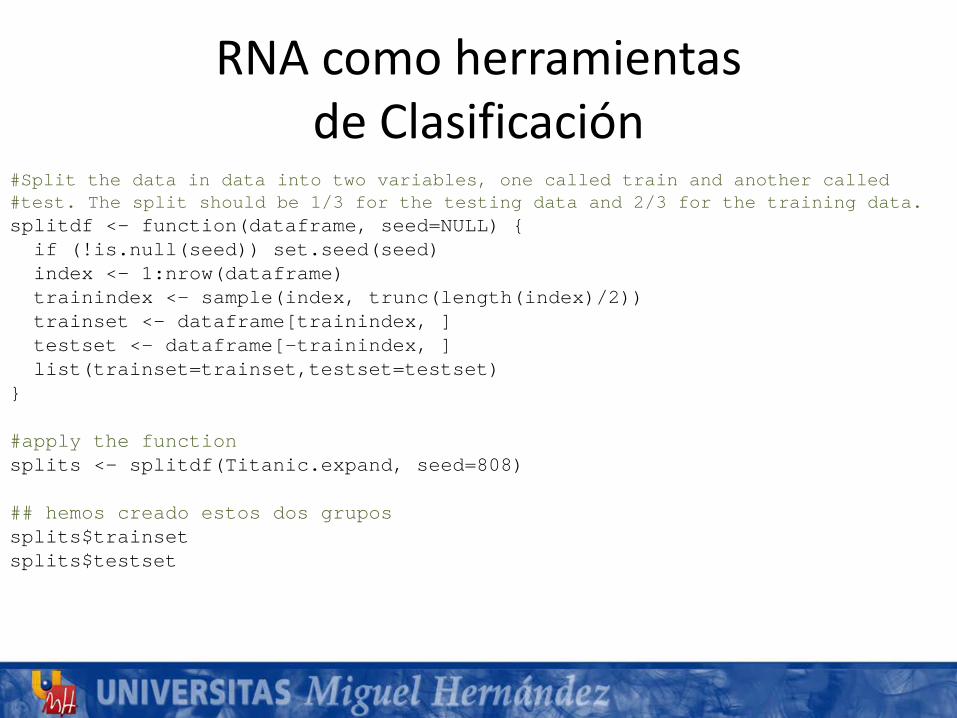
#Split the data in data into two variables, one called train and another called#test. The split should be 1/3 for the testing data and 2/3 for the training data.splitdf <- function(dataframe, seed=NULL) {if (!is.null(seed)) set.seed(seed)index <- 1:nrow(dataframe)trainindex <- sample(index, trunc(length(index)/2))trainset <- dataframe[trainindex, ]testset <- dataframe[-trainindex, ]list(trainset=trainset,testset=testset)

}

#apply the functionsplits <- splitdf(Titanic.expand, seed=808)

## hemos creado estos dos grupossplits$trainsetsplits$testset

RNA como herramientasde Clasificación

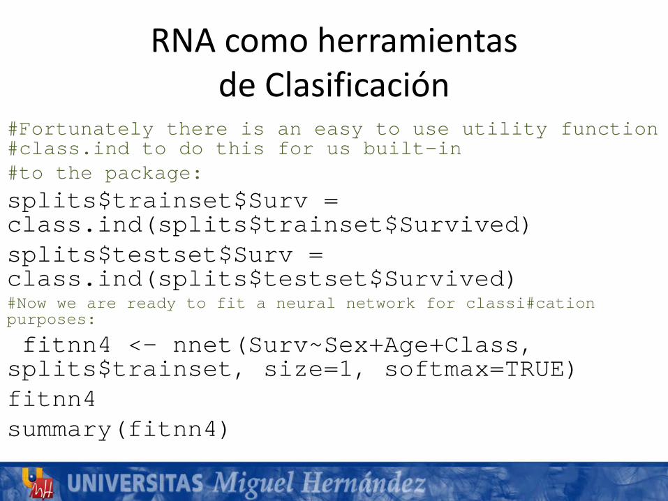
#Fortunately there is an easy to use utility function#class.ind to do this for us built-in#to the package:splits$trainset$Surv = class.ind(splits$trainset$Survived)splits$testset$Surv = class.ind(splits$testset$Survived)#Now we are ready to fit a neural network for classi#cationpurposes:

fitnn4 <- nnet(Surv~Sex+Age+Class, splits$trainset, size=1, softmax=TRUE)fitnn4summary(fitnn4)

RNA como herramientasde Clasificación

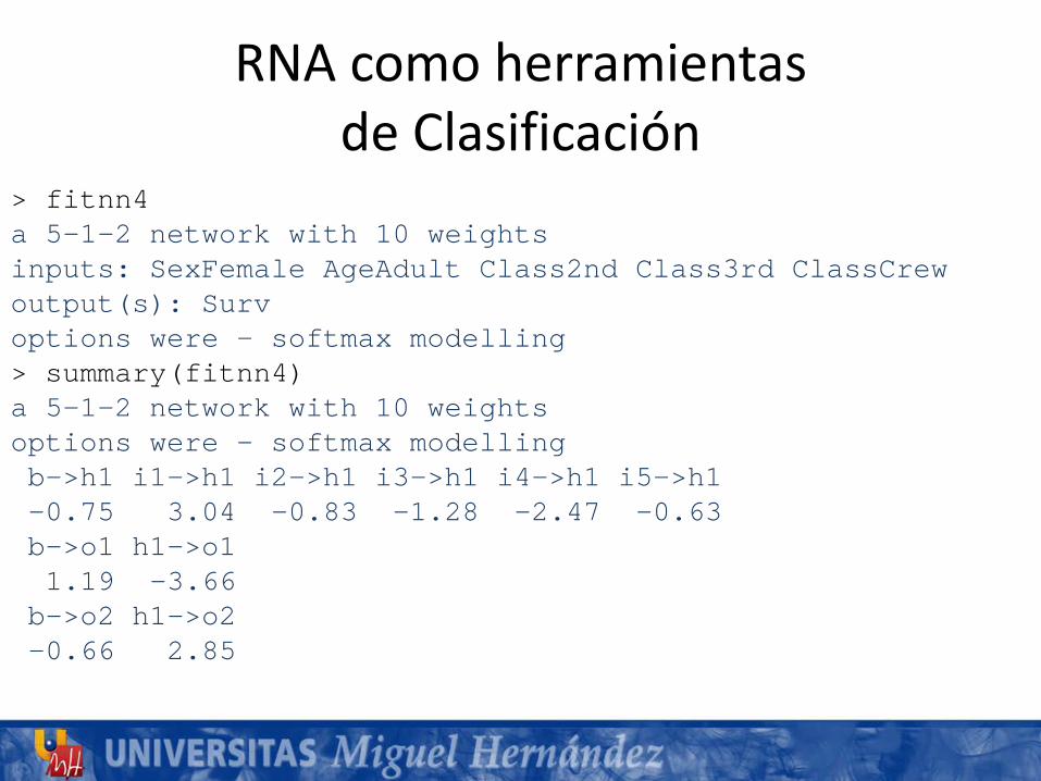
> fitnn4a 5-1-2 network with 10 weightsinputs: SexFemale AgeAdult Class2nd Class3rd ClassCrewoutput(s): Survoptions were - softmax modelling> summary(fitnn4)a 5-1-2 network with 10 weightsoptions were - softmax modellingb->h1 i1->h1 i2->h1 i3->h1 i4->h1 i5->h1 -0.75 3.04 -0.83 -1.28 -2.47 -0.63 b->o1 h1->o1 1.19 -3.66 b->o2 h1->o2 -0.66 2.85

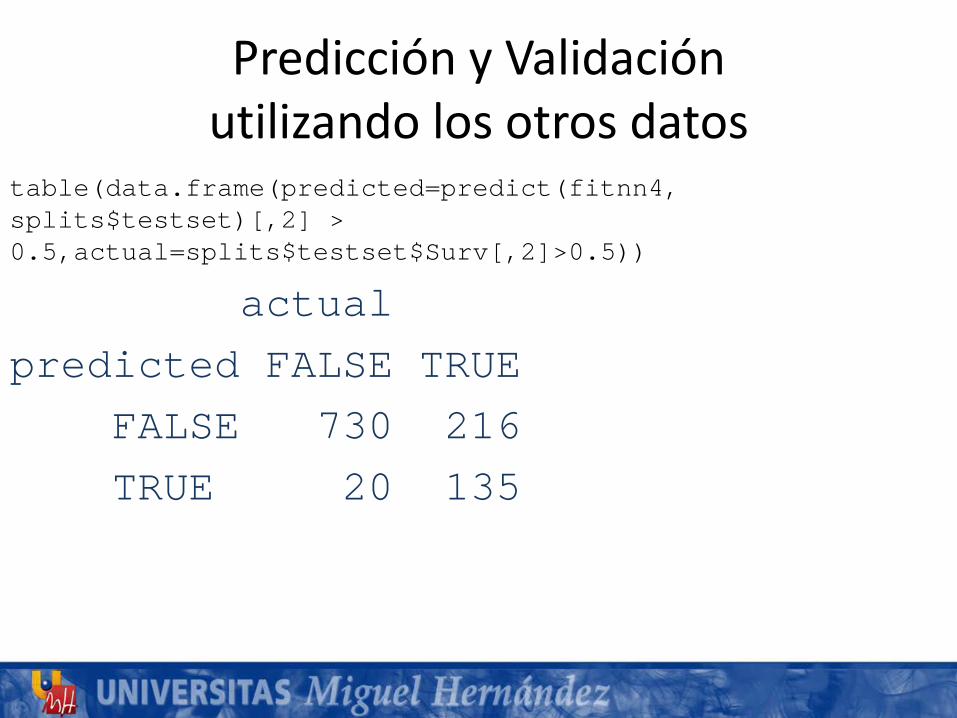
Predicción y Validaciónutilizando los otros datos

table(data.frame(predicted=predict(fitnn4, splits$testset)[,2] > 0.5,actual=splits$testset$Surv[,2]>0.5))

actual

predicted FALSE TRUE

FALSE 730 216

TRUE 20 135

Y la red sería tal que así:

#import the function from Githublibrary(devtools)source_url('https://gist.github.com/fawda123/7471137/raw/c720af2cea5f312717f020a09946800d55b8f45b/nnet_plot_update.r')

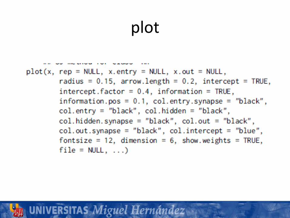
#plot each modelplot.nnet(fitnn4)

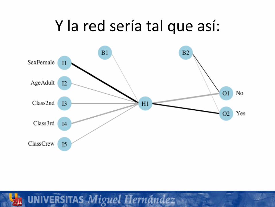
Y la red sería tal que así:

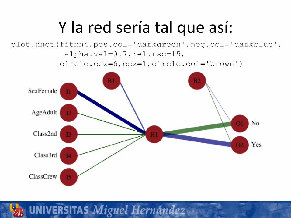
Y la red sería tal que así:plot.nnet(fitnn4,pos.col='darkgreen',neg.col='darkblue',

alpha.val=0.7,rel.rsc=15,circle.cex=6,cex=1,circle.col='brown')

EL EJEMPLO DE LAS DONACIONESUtilizando otra librería de R: neuralnet

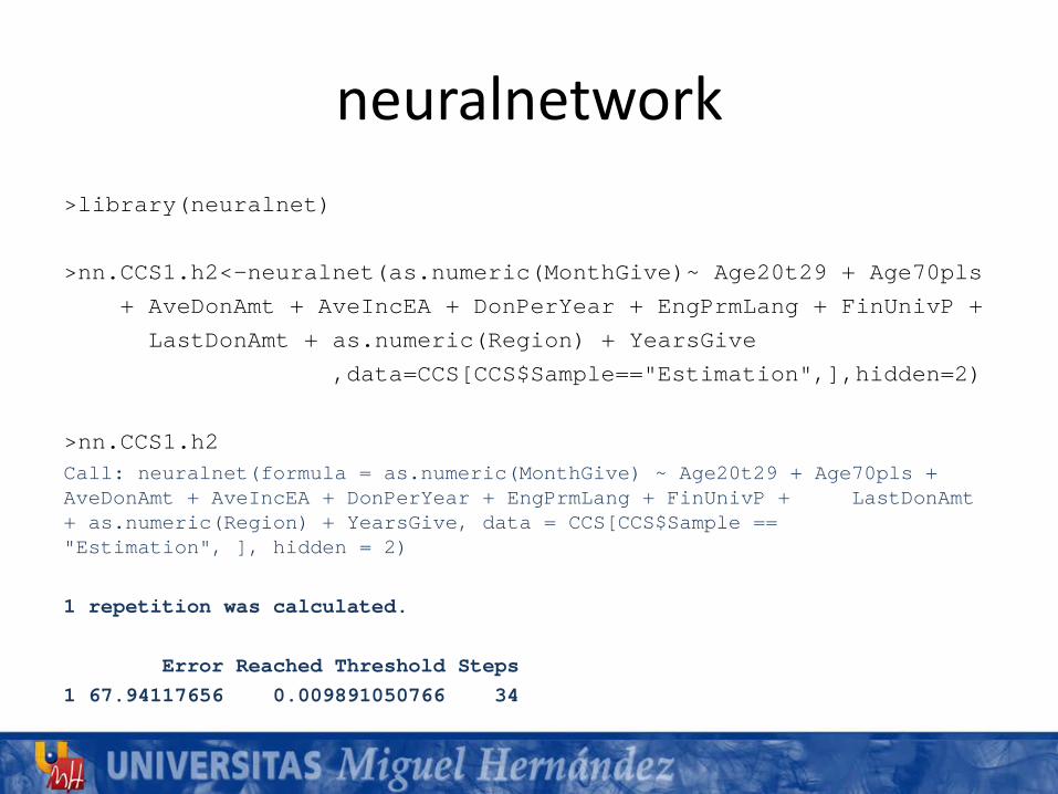
neuralnetwork>library(neuralnet)

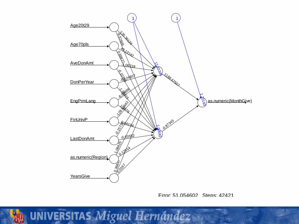
>nn.CCS1.h2<-neuralnet(as.numeric(MonthGive)~ Age20t29 + Age70pls

+ AveDonAmt + AveIncEA + DonPerYear + EngPrmLang + FinUnivP +

LastDonAmt + as.numeric(Region) + YearsGive

,data=CCS[CCS$Sample=="Estimation",],hidden=2)

>nn.CCS1.h2Call: neuralnet(formula = as.numeric(MonthGive) ~ Age20t29 + Age70pls + AveDonAmt + AveIncEA + DonPerYear + EngPrmLang + FinUnivP + LastDonAmt+ as.numeric(Region) + YearsGive, data = CCS[CCS$Sample == "Estimation", ], hidden = 2)

1 repetition was calculated.

Error Reached Threshold Steps1 67.94117656 0.009891050766 34

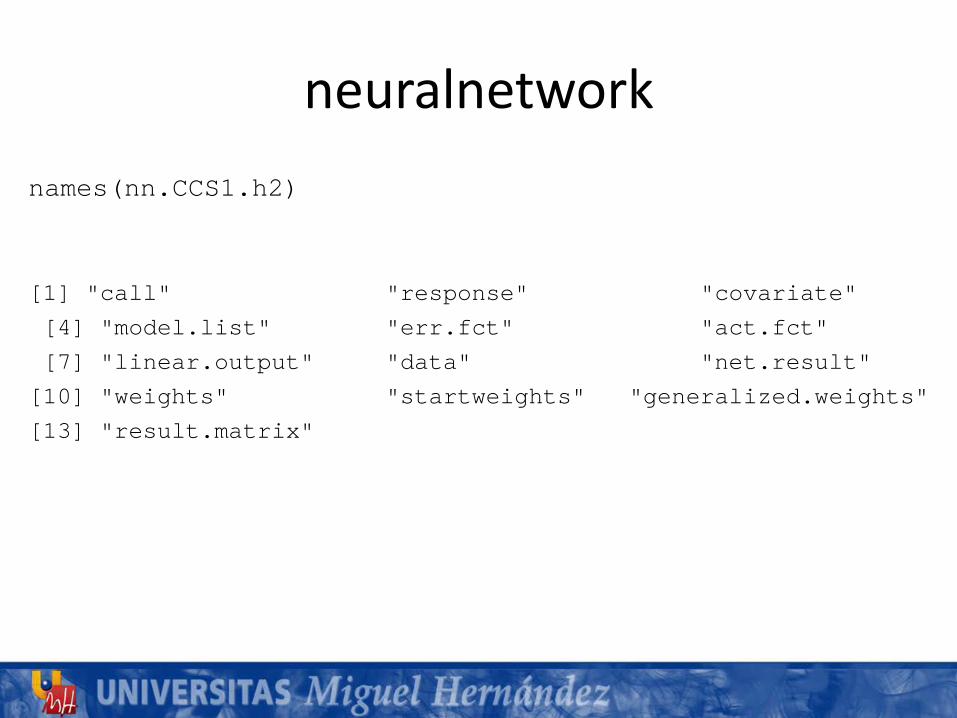
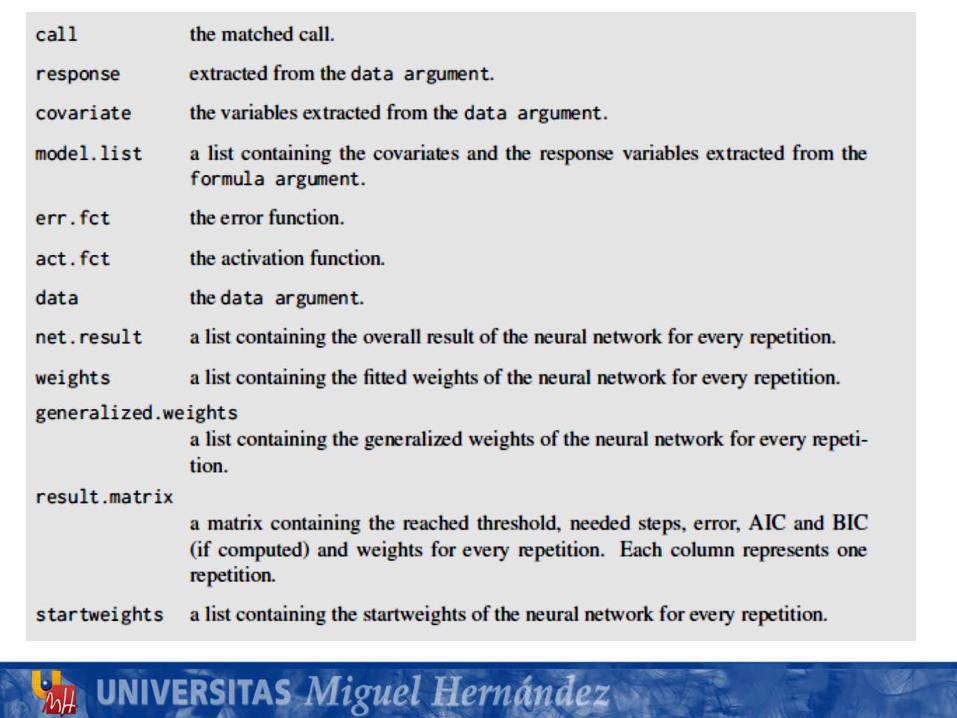
neuralnetworknames(nn.CCS1.h2)

[1] "call" "response" "covariate"

[4] "model.list" "err.fct" "act.fct"

[7] "linear.output" "data" "net.result"

[10] "weights" "startweights" "generalized.weights"

[13] "result.matrix"

neuralnetwork

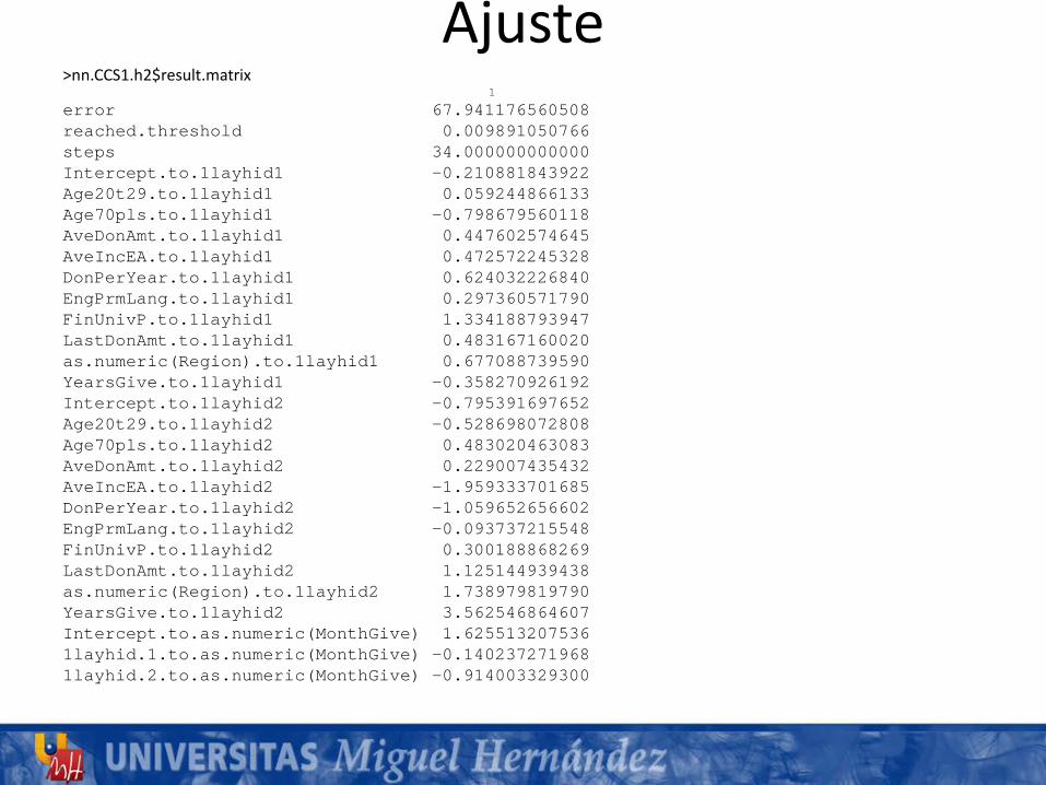
Ajuste>nn.CCS1.h2$result.matrix

1

error 67.941176560508reached.threshold 0.009891050766steps 34.000000000000Intercept.to.1layhid1 -0.210881843922Age20t29.to.1layhid1 0.059244866133Age70pls.to.1layhid1 -0.798679560118AveDonAmt.to.1layhid1 0.447602574645AveIncEA.to.1layhid1 0.472572245328DonPerYear.to.1layhid1 0.624032226840EngPrmLang.to.1layhid1 0.297360571790FinUnivP.to.1layhid1 1.334188793947LastDonAmt.to.1layhid1 0.483167160020as.numeric(Region).to.1layhid1 0.677088739590YearsGive.to.1layhid1 -0.358270926192Intercept.to.1layhid2 -0.795391697652Age20t29.to.1layhid2 -0.528698072808Age70pls.to.1layhid2 0.483020463083AveDonAmt.to.1layhid2 0.229007435432AveIncEA.to.1layhid2 -1.959333701685DonPerYear.to.1layhid2 -1.059652656602EngPrmLang.to.1layhid2 -0.093737215548FinUnivP.to.1layhid2 0.300188868269LastDonAmt.to.1layhid2 1.125144939438as.numeric(Region).to.1layhid2 1.738979819790YearsGive.to.1layhid2 3.562546864607Intercept.to.as.numeric(MonthGive) 1.6255132075361layhid.1.to.as.numeric(MonthGive) -0.1402372719681layhid.2.to.as.numeric(MonthGive) -0.914003329300

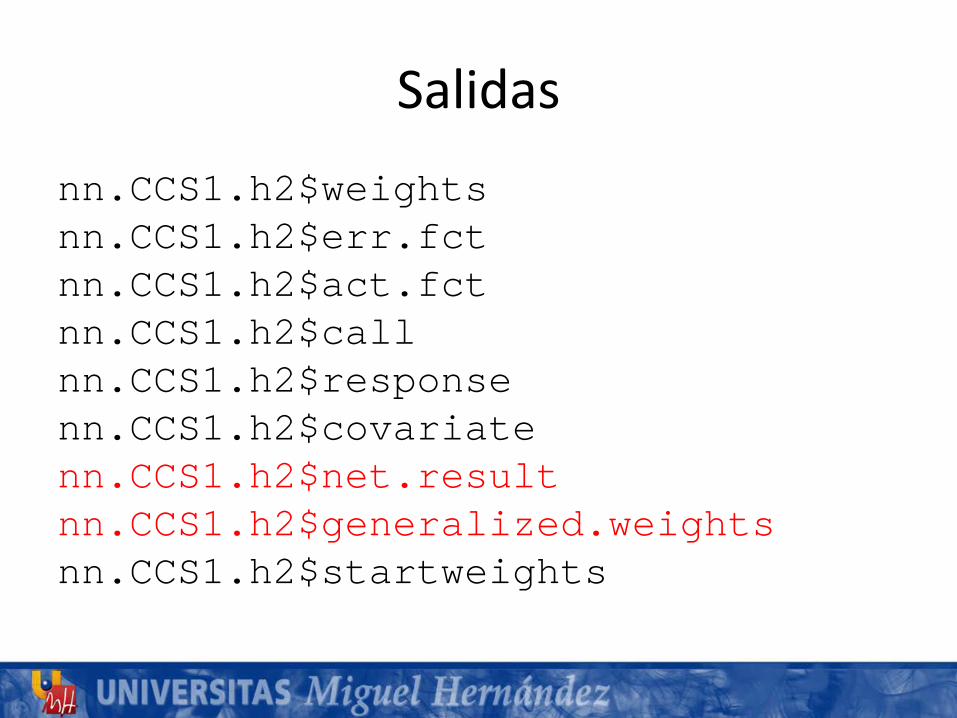
Salidasnn.CCS1.h2$weightsnn.CCS1.h2$err.fctnn.CCS1.h2$act.fctnn.CCS1.h2$callnn.CCS1.h2$responsenn.CCS1.h2$covariatenn.CCS1.h2$net.resultnn.CCS1.h2$generalized.weightsnn.CCS1.h2$startweights

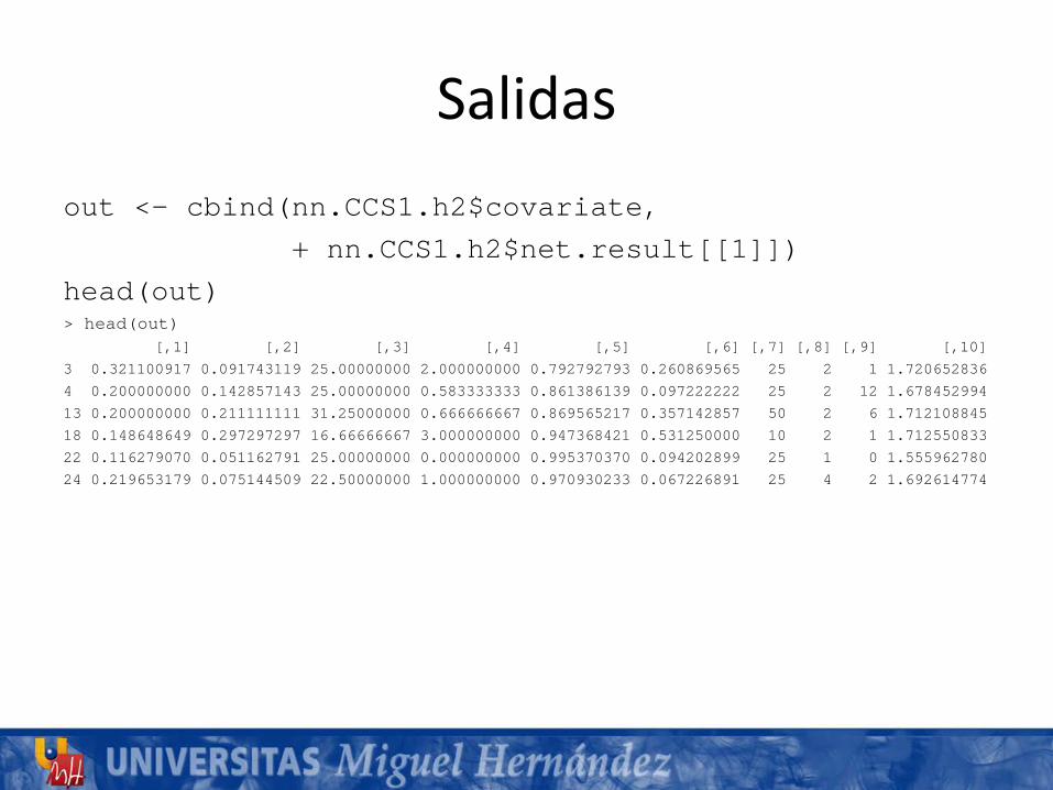
Salidasout <- cbind(nn.CCS1.h2$covariate,

+ nn.CCS1.h2$net.result[[1]])

head(out)> head(out)

[,1] [,2] [,3] [,4] [,5] [,6] [,7] [,8] [,9] [,10]

3 0.321100917 0.091743119 25.00000000 2.000000000 0.792792793 0.260869565 25 2 1 1.720652836

4 0.200000000 0.142857143 25.00000000 0.583333333 0.861386139 0.097222222 25 2 12 1.678452994

13 0.200000000 0.211111111 31.25000000 0.666666667 0.869565217 0.357142857 50 2 6 1.712108845

18 0.148648649 0.297297297 16.66666667 3.000000000 0.947368421 0.531250000 10 2 1 1.712550833

22 0.116279070 0.051162791 25.00000000 0.000000000 0.995370370 0.094202899 25 1 0 1.555962780

24 0.219653179 0.075144509 22.50000000 1.000000000 0.970930233 0.067226891 25 4 2 1.692614774

0.016

7

0.36

847

YearsGive

0.12814

1.08

425

as.numeric(Region)

-0.03552-0.15

716

LastDonAmt

0.64194

-128

.6864

2

FinUnivP

1.3676

-6.6965

6

EngPrmLang

-1.55815

-52.26817

DonPerYear

-0.10159

-1.06218AveDonAmt

0.69977

49.13142

Age70pls

-9.57605-135.36126

Age20t29

-0.8734

3

1188.67507

as.numeric(MonthGive)

1.5058217.83345

1

1.72193

1

Error: 51.054602 Steps: 42421

plot

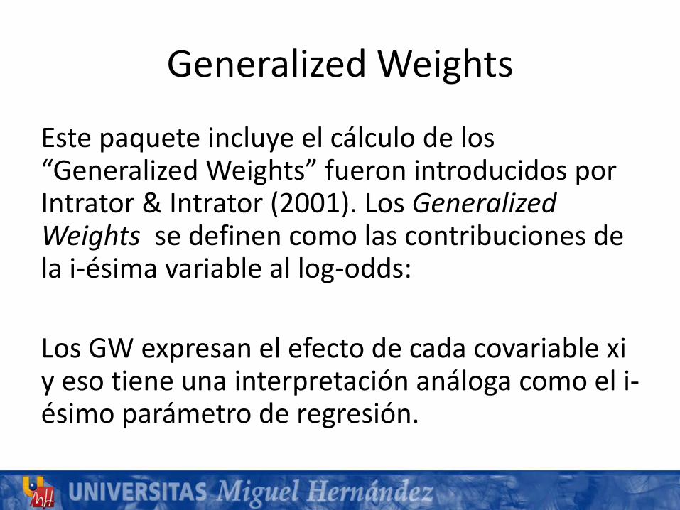
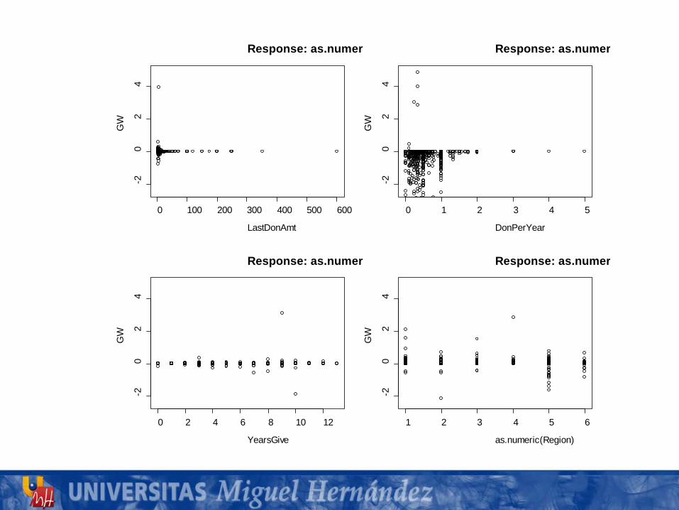
Generalized Weights

Este paquete incluye el cálculo de los “Generalized Weights” fueron introducidos por Intrator & Intrator (2001). Los GeneralizedWeights se definen como las contribuciones de la i-ésima variable al log-odds:

Los GW expresan el efecto de cada covariable xi y eso tiene una interpretación análoga como el i-ésimo parámetro de regresión.

0 100 200 300 400 500 600

-20

24

LastDonAmt

GW

Response: as.numer

0 1 2 3 4 5

-20

24

DonPerYear

GW

Response: as.numer

0 2 4 6 8 10 12

-20

24

YearsGive

GW

Response: as.numer

1 2 3 4 5 6

-20

24

as.numeric(Region)

GW

Response: as.numer

Y más cositas …

>compute>confidence.interval>prediction

BibliografíaBishop, C.M.: Neural Networks for Pattern Recognition. Oxford University Press, Oxford (2006)

http://halweb.uc3m.es/esp/Personal/personas/jmmarin/esp/DM/tema3dm.pdf

http://es.wikipedia.org/wiki/Red_neuronal_artificial

http://catarina.udlap.mx/u_dl_a/tales/documentos/lis/navarrete_g_j/capitulo2.pdf

http://avellano.usal.es/~lalonso/RNA/

Bibliografía