racionalizabilidad en juegos y coordinacion de …
TRANSCRIPT

UNIVERSIDAD DE CHILE
FACULTAD DE CIENCIAS FISICAS Y MATEMATICAS
DEPARTAMENTO DE INGENIERIA MATEMATICA
RACIONALIZABILIDAD EN JUEGOS Y COORDINACION DE
ANTICIPACIONES
TESIS PARA OPTAR AL GRADO DE DOCTOR EN CIENCIAS DE LA INGENIERIA
MENCION MODELACION MATEMATICA
EN COTUTELA CON LA ESCUELA DE ALTOS ESTUDIOS EN CIENCIAS SOCIALES
DE PARIS
PEDRO DANIEL JARA MORONI
PROFESOR GUIA :
RENE ALEJANDRO JOFRE CACERES
MIEMBROS DE LA COMISION:
ROGER GUESNERIE
GABRIEL DESGRANGES
MOHAMMED ALIUDDIN KHAN
SANTIAGO DE CHILE
NOVIEMBRE 2008


RESUMEN
En este trabajo evaluamos la estabilidad eductiva de los equilibrios de una clase de mod-
elos economicos compuestos de un continuo de agentes y de un estado agregado del mundo
sobre el cual los agentes tienen una influencia infinitesimal.
Usando como cuadro general una clase de juegos no atomicos con un continuo de agentes,
introducimos primero el concepto de racionalizabilidad. Cuando el pago de los jugadores
depende de las estrategias de los rivales solo a traves del valor de la integral del perfil de es-
trategias, proponemos una definicion del conjunto de estados (puntualmente) racionalizables
y entregamos una caracterizacion de estos conjuntos, a traves de la eliminacion iterativa de
puntos del conjunto de estados, para el caso en que el juego satisface hipotesis adecuadas de
continuidad y medibilidad de la funcion de pagos.
Definimos entonces la racionalidad fuerte (o estabilidad eductiva) como la unicidad de la
solucion racionalizable del sistema economico y estudiamos la relacion entre este concepto de
estabilidad y la estabilidad iterativa en anticipaciones. La caracterizacion obtenida para la
racionalizabilidad, nos permite explorar el enfoque local de la estabilidad de anticipaciones.
Demostramos que en presencia de complementariedad estrategica, la unicidad del equilib-
rio es equivalente a su estabilidad eductiva. La heterogeneidad de creencias no juega ningun
rol en la coordinacion de anticipaciones, pues la estabilidad eductiva resulta ser equivalente
la estabilidad iterativa en anticipaciones.
Por otro lado, en presencia de sustitutabilidad estrategica, si bien la estabilidad eductiva
es tambien equivalente la estabilidad iterativa en anticipaciones, la unicidad del equilibrio no
asegura su estabilidad global.
Estudiamos tambien un duopolio donde las firmas deciden en una primera etapa su ca-
pacidad de produccion y compiten secuencialmente en precios en una segunda etapa, en la
cual el rol de lıder es determinado aleatoriamente. Obtenemos en este contexto que el resul-
tado de equilibrio de Cournot puede ser sostenido como equilibrio perfecto en sub-juegos en
estrategias puras del juego completo. Obtenemos tambien que existe la posibilidad de encon-
trar equilibrios diferentes al de Cournot, como consecuencia del orden aleatorio del juego y
de lo atractivo que resulta el rol de seguidor en el sub-juego en precios. Finalmente, damos
una condicion suficiente para la existencia de tales equilibrios.
iii

ABSTRACT
In this work we evaluate the eductive stability of equilibria in a class of models that
feature a continuum of agents and an aggregate state of the world over which agents have an
infinitesimal influence.
Set in the framework of a class of games with a continuum of players, we first introduce the
concept of rationalizability. When the payoff of a player depends on his opponents strategies
only through the value of the integral of the strategy profile, we propose a definition for
the set of (point-) rationalizable states; we provide a characterization of such sets, through
the iterative elimination of points in the set of states, for the case where the game’s payoffs
function satisfies suitable continuity and measurability hypothesis.
We define strong rationality (or eductive stability) as the uniqueness of the rationalizable
solution of the economic system and we study the relation between this stability concept and
iterative expectational stability. The characterization obtained for rationalizability allows us
to explore the local viewpoint of expectational stability.
We prove that in the presence of strategic complementarities, uniqueness of equilibrium is
equivalent to its stability. Heterogeneity of beliefs plays no role in expectational coordination,
since eductive stability is equivalent to iterative expectational stability.
On the other hand in the presence of strategic substitutabilities, although eductive sta-
bility is as well equivalent to iterative expectational stability, uniqueness of equilibrium does
not assure its global stability.
We study in the last chapter a duopolistic model in which, first, firms engage simultane-
ously in capacity and compete sequentially in prices in a second stage, in which leadership is
determined randomly. We obtain in this context that the Cournot outcome can be sustained
as a pure strategy sub-game perfect Nash equilibrium of the whole game. We obtain as well
that it is possible to find equilibria in which firms produce strictly more than the Cournot
outcome, as a consequence of the random timing of the game and the attractiveness of be-
ing follower in the price sub-game. We give a sufficient condition to have existence of such
equilibria.
iv

AGRADECIMIENTOS
A mis Directores de Tesis Roger Guesnerie y Alejandro Jofre, por darme la oportunidad
de tan valiosa aventura.
Al Profesor Rafael Correa por todo su apoyo.
A los estudiantes y personal del DELTA y PSE; y del Departamento de Ingenierıa
Matematica de la Universidad de Chile.
A los futbolistas del PSE, del Club de la Pilsen y de las canchas de Antony, Francia.
A mis amigos de Chile y Francia, cuyo recibimiento entusiasta en cada una de mis idas
y vueltas nos hacıa sentir siempre en casa, imposible olvidar el primer ano en Paris junto a
Anneli y Eduardo ni los ultimos anos junto a Juan, Facundo, Olivier y el clan chileno, quienes
me ayudaron a sobrellevar los largos perıodos de separacion geografica de Javiera.
A mis suegros Francisco y Rebeca, a Pablo, Francisco y Marite.
Agradezco a mi hermano Pancho, a mi cunada Barbara y a mis padres Argos y Momy
por estar siempre presentes.
Quiero agradecer especialmente a Javiera, por su apoyo, su preocupacion, su paciencia y
su inmenso carino.
No puedo dejar de agradecer a los programas de becas de la Facultad de Ciencias Fısicas y
Matematicas de la Universidad de Chile y del Ministerio de Relaciones Exteriores de Francia;
al Nucleo Milenio Sistemas Complejos de Ingenierıa (actual Instituto Milenio), al Centro
de Modelamiento Matematico de la Universidad de Chile, al Departamento de Ingenierıa
Matematica de la Universidad de Chile, al DELTA (actual integrante de la EEP) y al College
de France; sin cuyo financiamiento mis estudios no habrıan sido posibles.
v

Though I know I’ll never lose affection
For people and things that went before,
I know I’ll often stop and think about them
In my life I love you more.
de In my life
Try to see it my way,
Only time will tell if I am right or I am wrong,
de We can work it out
The Beatles
vi

Contents
1. Introduction 1
2. Rationalizability in Games with a continuum of players 6
1. Introduction . . . . . . . . . . . . . . . . . . . . . . . . . . . . . . . . . . . . 10
2. Games With a Continuum of Players . . . . . . . . . . . . . . . . . . . . . . 16
2.1. Payoff Functions that Depend on the Integral of the Strategy Profile . 17
3. Point-Rationalizability . . . . . . . . . . . . . . . . . . . . . . . . . . . . . . 19
3.1. Point-Rationalizable Strategies . . . . . . . . . . . . . . . . . . . . . 20
3.2. Point-Rationalizable States . . . . . . . . . . . . . . . . . . . . . . . . 23
3.3. Point-Rationalizable Strategies vs. Point-Rationalizable States . . . . 34
3.4. Strongly Point Rational Equilibrium . . . . . . . . . . . . . . . . . . 36
4. Rationalizability vs Point-Rationalizability . . . . . . . . . . . . . . . . . . . 38
4.1. Forecasts over the set of states . . . . . . . . . . . . . . . . . . . . . . 38
4.2. More of Example 2.3 . . . . . . . . . . . . . . . . . . . . . . . . . . . 46
4.3. Forecasts over the set of strategies . . . . . . . . . . . . . . . . . . . . 48
4.4. Games with a continuum of players and finite strategy set . . . . . . 50
vii

5. Comments and Conclusions . . . . . . . . . . . . . . . . . . . . . . . . . . . 54
3. Strategic Complementarities vs Strategic Substitutabilities 56
1. Introduction . . . . . . . . . . . . . . . . . . . . . . . . . . . . . . . . . . . . 59
2. The canonical model and concepts. . . . . . . . . . . . . . . . . . . . . . . . 61
2.1. Games with a continuum of players . . . . . . . . . . . . . . . . . . . 61
2.2. Economic System with a continuum of agents . . . . . . . . . . . . . 63
3. Rationalizability and the “eductive learning viewpoint”. . . . . . . . . . . . . 66
3.1. Rationalizability : the game viewpoint. . . . . . . . . . . . . . . . . . 66
3.2. Rationalizability : an “economic” viewpoint. . . . . . . . . . . . . . . 67
4. Rationalizable outcomes, Equilibria and Stability . . . . . . . . . . . . . . . 71
4.1. The global viewpoint. . . . . . . . . . . . . . . . . . . . . . . . . . . . 71
4.2. The local viewpoint. . . . . . . . . . . . . . . . . . . . . . . . . . . . 73
5. Economic games with strategic complementarities or substitutabilities. . . . 75
5.1. Economic games with strategic complementarities. . . . . . . . . . . . 75
5.2. Economic games with Strategic Substitutabilities . . . . . . . . . . . 81
6. The differentiable case. . . . . . . . . . . . . . . . . . . . . . . . . . . . . . . 86
6.1. The strategic complementarities case. . . . . . . . . . . . . . . . . . . 86
6.2. The strategic substitutabilities case. . . . . . . . . . . . . . . . . . . . 88
7. Comments and Conclusions . . . . . . . . . . . . . . . . . . . . . . . . . . . 88
4. The Cournot Outcome as the Result of Price Competition 97
1. Introduction . . . . . . . . . . . . . . . . . . . . . . . . . . . . . . . . . . . . 97
2. The Model . . . . . . . . . . . . . . . . . . . . . . . . . . . . . . . . . . . . . 99
3. Equilibrium With Simultaneous Price-Setting Subgame . . . . . . . . . . . . 101
4. Equilibria With Sequential Price-setting Subgame . . . . . . . . . . . . . . . 103
viii
ix
4.1. Price-setting subgame . . . . . . . . . . . . . . . . . . . . . . . . . . 103
4.2. Capacity Setting Reduced Game . . . . . . . . . . . . . . . . . . . . 112
5. Concluding Remarks . . . . . . . . . . . . . . . . . . . . . . . . . . . . . . . 119
5. Conclusions 121
CHAPTER 1
Introduction
In recent years, significant effort is being directed to give formal justifications for the
Rational Expectations Hypothesis in economics. In this line of research the “eductive” and
“learning” viewpoints of rational expectations put emphasis into the idea that Rational
Expectations Equilibria should be explained rather than assumed. Our interest is on the
eductive explanations, which rely on the analysis of mental processes of the economic system’s
participating agents that seek to forecast, not directly the outcome itself of the system, but the
forecasts of forecasts of the other agents, in order to anticipate such an outcome. This is, even
in the case in which there is no uncertainty about the situation in which economic agents are
immersed (what we would call structural uncertainty) there is always strategic uncertainty,
agents have to rely on forecasts to justify their actions. One important attempt to set a
clear set of assumptions that justify this concept is that of Strongly Rational Expectations
Equilibrium proposed by Guesnerie (1992, 2002). Guesnerie transposes in economic contexts
the ideas that in game-theoretical frameworks are behind the concepts of rationalizability, in
order to ask whether rational economic agents may “educe” a so-called Rational Expectations
Equilibrium. These ideas rely on two basic hypothesis: individual rationality and common
knowledge. The emphasis is put on the formation of beliefs through a process that rules out
unreasonable outcomes following these two hypothesis.
Bernheim (1984) and Pearce (1984) introduced the concept of Rationalizable Strategies,
in the context of games with a finite number of players, as the adequate solution concept when
players are modeled as rational agents that take decisions independently and in ignorance
of the strategies adopted by the other players 1. These agents must rely in forecasts and
an internally consistent system of beliefs that justify such forecasts. Rationality of players
1See as well the papers by Tan and da Costa Werlang (1988) and Basu and Weibull (1991) for character-izations and justifications of Rationalizable Solutions
1

CHAPTER 1. INTRODUCTION
means that players maximize expected utility subject to some prior regarding the choice of
their opponents, this prior must not contradict any information that they might have and
players know that their opponents maximize expected utility and rely on such priors. We
may say that players are rational and that rationality is common knowledge, they optimize
and it is in their interest to use the correct forecast.
In Bernheim (1984), Rationalizability is introduced through the definition of a consistent
system of beliefs in the context of general normal form games, while Pearce (1984) focuses in
an iterative procedure of elimination of non-optimal strategies in the special case of games
where the sets of actions are finite. The two papers can be merged using Proposition 3.2 in
Bernheim (1984) (see page 8 of this report), which states that for games where the strategy
sets are compact subsets of Rn and the payoff functions are continuous, then the set of
Rationalizable Strategies is characterized by two equivalent definitions:
1. It is the result of the iterative elimination of non-best-reply strategies2.
2. It is the largest set of strategy profiles that satisfies being a fixed point of the process
of elimination of non-best-replies.
Under these premises, the formation of beliefs and the plausibility of equilibrium outcome
has been analyzed in a series of works (Desgranges and Heinemann 2005, Guesnerie 2005,
Desgranges and Gauthier 2004, Guesnerie 2002, Guesnerie 1992, among others) by setting
an economic situation into a game-theoretical framework in order to use the concept of
Rationalizability as a stability test for equilibria, regarding forecasts. In an economic system,
following Guesnerie (1992), an equilibrium is said to be Strongly Rational or Eductively
Stable if it is the unique outcome associated to the set of Rationalizable Solutions of the
game form of such a system. From the expectations formation point of view, the economic
agents should conclude that the only possible outcome of the system must be it’s unique
equilibrium, thus justifying the rational expectations hypothesis. It is in these good cases,
as stated by Guesnerie, that “the rational expectations forecast is the necessary outcome of
agents’ mental activities which have clear and appealing grounds”. We may then say that
agents will coordinate in the equilibrium.
Eductive Stability, however, has been studied mainly in models that feature a continuum
of agents, many of which have macroeconomic inspirations, to model situations in which
agents are “small” with respect to the economy, in the sense that they have no individual
influence over the economic system in which they are immersed. Examples of these models
can be found in the articles mentioned above as well as in Evans and Guesnerie (1993), where
the authors study Eductive Stability in a general linear model of Rational Expectations or
2Strategies that are never the result of individual payoff maximization.
2

CHAPTER 1. INTRODUCTION
Evans and Guesnerie (2003, 2005) for dynamics in macroeconomics. See as well the book by
Chamley (2004), whose second part treats Coordination based on eductive stability. These
and other works that feature a continuum of agents, including the seminal work by Guesnerie
(1992), feature intuitive and/or context-specific, for the considered model, definitions of
Rationalizability. It is then of primary interest to present a model of game that first, captures
the features of these economic models and second, allows us to provide a general theoretical
framework in which we can study Rationalizability as a natural extension of the finite player
games described above.
In the first part of this presentation, Chapter 2, we aim to link the established game-
theoretical concepts to its’ economic applications in macroeconomics and economic models.
We present a general framework of a game with a continuum of players over which the ideas
of Bernheim and Pearce can be formally described and characterized. We define there the
concepts of Rationalizable and Point-Rationalizable States, and Point-Rationalizable Strate-
gies. The definition of (standard) Rationalizable Strategies for games with a continuum of
players is nevertheless a more delicate task. We give a formal definition and characterization
for this last concept in the particular case where the set of actions is finite. This framework
allows then to work with the concept of Rationalizability in a very general setting. It is as
well a framework that encompasses a large literature of specific economic and macroeconomic
models including the ones already mentioned (see also Townsend (1978)). With this we aim
as well to put together together, explicitly, lines of economic research that seemed to be
unrelated in the literature until know, as are macroeconomics and games with a continuum
of agents in a general setting. Then, following Guesnerie (1992) and using Rationalizability
as a test for stability of equilibria, we can formally define and study Eductive Stability, in a
general framework.
In Chapter 3 we make use of the framework, definitions and characterization of Rational-
izable Solutions presented in Chapter 2, to address stability of equilibria (local and global).
Part of our interest is the comparison between the already mentioned stability concept of
Eductive Stability and Expectational Stability (Lucas 1978; DeCanio 1979). Expectational
stability is related to the iterations of a best response mapping and can therefore be inter-
preted as a process that tends to seek outcomes where agents have homogeneous expectations
as opposed to Strong Rationality in which we allow agents to have heterogeneous expecta-
tions. The characterizations of rationalizability obtained in Chapter 2 allow us to assess local
eductive stability of equilibria as the result of the eductive process described in that Chapter,
started from a neighborhood of an equilibrium. The comparison between these two stability
concepts is stressed then as well from this local viewpoint in Chapter 3.
Further on we will explore the implications over stability of equilibria of the presence
of a specific structure in the underlying game form of the economic model. We endow the
3

CHAPTER 1. INTRODUCTION
game-theoretical model of Chapter 2 with a lattice structure in order to introduce strategic
complementarity or substitutability and study how the economic setting inherits this ordered
structure. We show that it is possible to go from a strategic point of view to a model in which
there is an aggregate value that summarizes all the information that agents need in order to
take a decision. This is, the ordered structure of a strategy profile set (a set of functions) is
passed on to the set of aggregate values obtained from such profiles.
Once these tools are established we argue that the presence of Strategic Complementarities
helps expectational coordination. The results in the literature of strategic complementari-
ties in games with a finite number of players (Milgrom and Roberts 1990; Vives 1990) are
extended, as expected, for the case of a continuum of players. Indeed, we will see in Chapter
3 that under such a setting, uniqueness of equilibrium is a sufficient condition for it to be
Eductively Stable. We will show as well that this equilibrium is Eductively Stable if and only
if it is Iterative Expectationaly Stable, simplifying the stability test for the former concept.
On the other hand, although the presence of Strategic Substitutabilties gives some more
structure to the stability tests, we can not say as much of stability of equilibria in this second
case. Uniqueness of equilibrium does not give its’ stability, nor eductvie nor iteratively ex-
pectational, but we show that the study of the second iterate of a best response type mapping
may give some light. In this case, if the second iterate of the mapping has a unique fixed
point, then we can say that the there is a unique rationalizable solution and consequently
it will be a strongly rational equilibrium. We also have that iterative expectational stability
and eductive stability are equivalent (we have one if and only if we have the other) and so
heterogeneity of expectations is not relevant under the strategic substitutabilities setting.
Chapter 4 constitutes a short essay on duopolistic competition. Inspired by the work of
Kreps and Scheinkman (1983), an exercise is proposed in order to reestablish the existence
of pure strategy equilibrium in a price competition capacity constrained duopoly. The main
issue in the original paper of Kreps and Scheinkman was to clarify the difference between
Cournot and Bertrand competition, understood as competition on quantities opposed to
competition on prices. The authors argue that the significant differences between these two
approaches is not only the strategy space of the game (quantities vs. prices), but that timing
of decision was relevant. To illustrate this, they present a duopoly in which price competition
comes after the decision on production 3, thus reversing the order of decision from Bertrand
competition where production is decided after prices are revealed, concluding that the whole
game had as outcome the Cournot quantities and prices, implying that both: competition
3Although in the literature that has followed this article, the emphasis has been made in the interpretationthat says that in the quantity setting game the competition is in capacity and not production, we use theterminology of the authors (production). Even more, using the interpretation of capacity setting in theirmodel would imply that: 1. there is no cost of production in the second stage when the decision on quantitiesis made first, and 2. the interpretation of quantity changes from one game to the other, production in theBertrand game, capacity in the reversed game. We leave the interpretation to the reader.
4
CHAPTER 1. INTRODUCTION
on prices and production following the realization of the demand, are required for perfectly
competitive outcomes as in the Bertrand approach.
However, for a non negligible set of pairs of productions quantities, the capacity con-
strained price subgame had no pure strategy equilibrium. This inspires the exercise presented
in this Chapter. We seek for pure strategy outcomes since they are economically more perti-
nent. The second stage subgame is modified and price competition is turned to be sequential
in order to restore pure strategies at equilibrium and hopefully in the whole game-tree. Since
in the related literature there has been as well some emphasis on the competitive outcome
as the result of capacity constrained price competition, this issue is also partially assessed;
we give a condition that allows to find equilibria that deliver quantities strictly greater than
those that emerge at the Cournot equilibrium (see Section 1 and Subsection 4.2 of Chapter
4). In previous works, non Cournot outcomes are found by departing from the setting of
Kreps and Scheinkman (1983). In the present work there are no changes in the assumptions
of demand rationing, nor on properties of the costs functions.
Structure of the Thesis
The report consist of three chapters, each one of which contains an article that has been
submitted to international journals and/or conferences. The results of Chapter 2 are avail-
able as a working paper at the PARIS SCHOOL OF ECONOMICS, PARIS, FRANCE and
as a technical report at the CENTER OF MATHEMATICAL MODELING, SANTIAGO,
CHILE; they have been presented in the THIRD WORLD CONGRESS OF THE GAME
THEORY SOCIETY and the 2008 EUROPEAN MEETING OF THE ECONOMETRIC
SOCIETY and at several seminars. A preliminary version of an article with the results of
Chapter 3 has been presented in the IESE CONFERENCE ON COMPLEMENTARITIES
AND INFORMATION and at several seminars. An abridged version of the results of Chap-
ter 4 are available as a working paper at the PARIS SCHOOL OF ECONOMICS, PARIS,
FRANCE and as a technical report at the CENTER OF MATHEMATICAL MODELING,
SANTIAGO, CHILE; they have been presented at the 2007 CONFERENCE OF THE SO-
CIETY FOR THE ADVANCEMENT OF ECONOMIC THEORY. Chapters 2 and 3 include
the full text of each publication, preceded by an introductory section. Al chapters include a
reference to the most recent version of each article. We close the presentation with conclusions
and the bibliography of the thesis.
5

CHAPTER 2
Rationalizability in Games with a
continuum of players
Introductory Notes
In this chapter we present a framework in which it is possible to define the concept of
rationalizability in the context of economic models that feature a continuum of agents and
to obtain characterizations of the sets of rationalizable solutions. We introduce a suitable
class of non-atomic games and explore this concept. Rationalizability has been defined in
finite player games by Bernheim (1984) and Pearce (1984). For the sake of completeness, we
summarize below the presentation in Bernheim.
A finite player game is a triplet⟨J,(Si)i∈J ,(πi)i∈J
⟩where J is a finite set of players, for
each i ∈ J , Si ⊆ Rn are sets of strategies or actions available for the players and the functions
πi :∏
i∈J Si → R give the payoff for each player and each profile of strategies.
The key concept of a game is that of Nash Equilibrium. A strategy profile s∗ ∈∏
i∈J Si is
a Nash Equilibrium of a game if for each player, his strategy s∗i is a maximizer of the payoff
function, given the strategies of his opponents:
∀ i ∈ J, πi(s∗) ≥ πi
(y, s∗−i
)∀y ∈ Si
To define Rationalizable Strategies, Bernheim formalizes the idea of system of beliefs and
defines a consistent system of beliefs. A system of beliefs for a player i ∈ J represents
the possible forecasts of the player concerning the forecasts over forecasts of his opponents,
concerning what any player would do. These forecasts take the form of borel measurable
subsets of the players’ strategy sets. If a system of beliefs gives only singletons, then he
calls it a system of point beliefs. A consistent system of beliefs simply emphasizes the idea
6

CHAPTER 2. RATIONALIZABILITY
that players should consider in their forecast that the opponents are rational and so are
optimizing with respect to some forecasts of their own. Rationality and common knowledge
of rationality then imply that a system of beliefs must satisfy a consistent condition stressed
as follows:
If player i thinks it is possible that player i1 thinks it is possible that,. . .
player in−1 thinks it is possible that player in might take an action sin , then
sin must be a best response to some subjective distribution over in’s opponents’
strategies, where anything receiving nonzero probability in this distribution must
be something which i thinks it is possible that i1 thinks it is possible that,. . .
in−1 thinks it is possible that in thinks his opponents might possibly do.1
With these tools, Bernheim defines Rationalizability as follows.
Definition 2.1 (Bernheim (1984)). si is a Rationalizable Strategy for player i iff there exists
some consistent system of beliefs for player i and some probability measure µ−i ∈∏
j 6=i P(Sj),
such that si ∈ Bri(µ−i), and µ−i is a subjective probability distribution that gives zero
probability to actions of the opponents of i that are ruled out by this system of beliefs. In
the particular case where the system is of point beliefs, we say that si is a point rationalizable
strategy.
If the players of a game take actions independently and in ignorance of the actions taken
by their opponents, it is pertinent to consider the mapping Bri :∏
j 6=i P(Sj) ⇒ Si that
assigns to each product probability measure µ−i over the product borel field, the set of
expected utility maximizers:
Bri(µ−i) := argmaxy∈Si Eµ−i [πi(y, s−i)]
For B =∏
j∈J B(Sj), we define a mapping R : B → B that eliminates strategies that are not
expected utility maximizers with respect to (subjective) probability measures whose supports
are contained in certain corresponding subsets∏
j 6=i Projj(H) ⊆ S−i for each player i ∈ J :
R(H) :=∏i∈J
⋃µ−i∈
∏j 6=i P(Projj(H))
Bri(µ−i)
The set R(H) contains all and only strategy profiles that can be obtained from the indepen-
dent actions of players that react optimally to some prior with support on the projection of
the set H over the product set of strategy profiles of the opponents.
1Taken form Bernheim (1984) p. 1014.
7
CHAPTER 2. RATIONALIZABILITY
Call S ≡∏
j∈J Sj. The following is the characterization, using the mapping R, of Ratio-
nalizable Strategies for a game as the one described above.
Proposition 2.2 (Bernheim, 1984). In a game with continuous payoff functions and compact
strategy sets, the set of Rationalizable Strategies, RS, is characterized as follows:
RS is the maximal subset H ⊆ S such that R(H) = H
RS ≡⋂t≥0
Rt(S)
The proposition states that the set of Rationalizable Strategies is the result of the it-
erative elimination of strategies that are not best-replies to forecasts considering all of the
remaining strategy profiles. There is another definition on the paper of Bernheim, that of
Point-Rationalizable Strategies, that considers only forecasts as points in the strategy sets
instead of probability assessments. The characterizations are analogous to the ones presented
in Proposition 2.2 but considering only strategy profiles instead of probability measures at
the best reply correspondence level.
Care is needed when we pass from this setting to a setting in which the player set is no
longer finite, but an interval of R, this is the principal issue to be treated in this Chapter.
8
CHAPTER 2. RATIONALIZABILITY
Full Paper. Current version: Jara-Moroni (2008b)
Rationalizability in Games with a
continuum of players
Abstract
The concept of Rationalizability has been used in the last fifteen years to study
stability of equilibria on models with continuum of agents such as standard com-
petitive markets, macroeconomic dynamics and currency attacks. However, Ra-
tionalizability has been formally defined in a general setting only for games with a
finite number of players and there is no general definition for Rationalizability in
the case of games with continuum of players. In this work, we propose a definition
for Point-Rationalizable Strategies in the context of Non-Atomic Noncooperative
Games with a Continuum of Players. In a special class of these games where
the payoff of a player depends only on his own strategy and an aggregate value
that represents the state of the game, state that is obtained from the actions
of all the players, we define the sets of Point-Rationalizable States and Ratio-
nalizable States. These last sets are characterized and some of their properties
are explored. We study as well standard Rationalizability in a subclass of these
games. We present an exploratory framework that encompasses the previously
mentioned models, over which we can link the established theory and its’ macroe-
conomic applications on stability properties of equilibria.
Keywords: Rationalizable Strategies, Non-atomic Games, Expectational Coor-
dination, Rational Expectations, Eductive Stability, Strong Rationality.
JEL Classification: D84, C72, C62.
9
CHAPTER 2. RATIONALIZABILITY
1 Introduction
The concept of Strong Rationality was first introduced by Guesnerie (1992) in a model
of a standard market with a continuum of producers. An equilibrium of the market is there
said to be Strongly Rational, or Eductively Stable, if it is the only Rationalizable Solution
of the economic system. Inspired in the work of Muth (1961), the purpose of such an
exercise was to give a rationale for the Rational Expectations Hypothesis. Strong rationality
has been studied as well in macroeconomic models in terms of stability of equilibria. See
for instance Evans and Guesnerie (1993), where they study Eductive Stability in a general
linear model of Rational Expectations or Evans and Guesnerie (2003, 2005) for dynamics in
macroeconomics. More examples of applications of Strong Rationality can be found in the
recent book by Chamley (2004) where he presents models of Stag Hunts in the context of
coordination in games with strategic complementarities.
The Rationalizable Solution of the economic system assessed by Guesnerie in the definition
of Strong Rationality, refers to the concept of Rationalizable Strategies as defined by Pearce
(1984) in the context of games with a finite number of players and finite sets of strategies.
Rationalizable Strategies were formally introduced by Bernheim (1984) and Pearce (1984) as
the “adequate” solution concept under the premises that players are rational utility maximiz-
ers that take decisions independently and that rationality is common knowledge. Adequate
because Rationalizable Strategy Profiles are outcomes of a game that cannot be discarded
based only on agents’ rationality and common knowledge. The work of Pearce focused mainly
in refinements of equilibria of extensive form finite games, while Bernheim gave a definition
and characterization in the context of general normal form games, along with comparison
between the set of Nash Equilibria and the set of Rationalizable Strategy Profiles. In both
papers and later treatments, however, the definition and characterization of rationalizable
“solutions” were developed for games with a finite number of players.
On the other hand, each one of the works that are mentioned in the first paragraph of
this introduction including the seminal work by Guesnerie (1992), feature intuitive and/or
context-specific definitions of the concept of Rationalizable Solution, adapting the original
definitions and characterizations of Rationalizable Strategies, based on the intuitions behind
them, to models with a continuum of agents. It is this gap between the established theory and
its’ economic applications that motivate this work. Since there is no established definition
for Rationalizable Strategies, or Rationalizability for what matters, in a general framework
with a continuum of agents, in this paper then we link the game-theoretical concept of
Rationalizability to its’ applications in macroeconomics and economic models, proposing a
general definition in the context of games with a continuum of players.
10

CHAPTER 2. RATIONALIZABILITY
To motivate this presentation let us describe the model and illustrate how the Rational-
izability concept is presented in Guesnerie’s (1992) work.
Example 2.3. Consider that we have a group of farmers, represented by the [0, 1] ≡ I
interval, that participate in a market in which production decisions are taken one period
before production is sold. Each farmer i ∈ I has a cost function ci : R+ → R. The
price p at which the good is sold is obtained from the (given) inverse demand function
P : R+ → [0, pmax] evaluated in total aggregate production p = P(∫
q(i) di)
where q(i) is
farmer i’s production. Since an individual change in production does not change the value
of the price, the product is sold at price-taking behavior, so each farmer i ∈ I maximizes
his payoff function u(i, · , · ) : R+ × [0, pmax] → R defined by u(i, q(i) , p) ≡ pq(i) − ci(q(i)).An equilibrium of this system is a price p∗ such that p∗ = P
(∫q∗(i) di
)and u(i, q∗(i) , p∗) ≥
u(i, q, p∗) ∀ q ∈ R, ∀ i ∈ I.
At the moment of taking the production decision, farmers do not actually know the value
of the price at which their production will be sold. Consequently they have to rely on forecasts
of the price or of the production decision of the other farmers. The concept in scrutiny in
our work is related to how this (these) forecast(s) is (are) generated.
Forecasts of farmers should be rational in the sense that no unreasonable price should be
given positive probability of being achieved. It is in this setting that Guesnerie introduces
the concept of strong rationality or eductive stability 2 as the uniqueness of rationalizable
prices which are obtained from the elimination of the unreasonable forecasts of possible
outcomes. To obtain these rationalizable prices, Guesnerie describes, in what he calls the
eductive procedure, how the unreasonable prices can be eliminated using an iterative process
of elimination of non-best-response strategies.
Now let us illustrate how the eductive process works in this setting. From the farmers
problem we can obtain for each farmer his supply function s(i, · ) : [0, pmax] → R+. The
structure of the payoff function implies that for a given forecast µ of a farmer i over the value of
the price, his optimal production is obtained evaluating his supply function in the expectation
under µ of the price, Eµ [p] : s(i,Eµ [p]). Farmers know that a price higher than pmax gives
no demand and so prices higher than those are unreasonable. Since all farmers can obtain
this conclusion, all farmers know that the other farmers should not have forecasts that give
positive weight to prices that are greater than pmax. The expectation of each of the farmers’
forecasts then cannot be greater than pmax and so under necessary measurability hypothesis
we can claim that aggregate supply can not be greater than S(pmax) =∫ 1
0s(i, pmax) di.
Since all farmers know that aggregate supply can not be greater than S(pmax), they know
2An equilibrium of an economic system is said to be strongly rational or eductively stable if it is the onlyRationalizable outcome of the system. We will refer equivalently to outcomes as begin strongly rational oreductively stable.
11

CHAPTER 2. RATIONALIZABILITY
then that the price, obtained through the inverse demand function, can not be smaller than
p1min = P (S(pmax)). All farmers know then that forecasts are constrained by the interval
[p1min, pmax]. They have discarded all the prices above pmax and below p1
min. This same
reasoning can be made now starting from this new interval.
-
6
�
?
q
p
!!!!
!!!!
!!!!
!!!!
!!
@@@@@@@@@@@@@@@
p∗
q∗
p1min
pmax6p2
max
P−1(p)�� S(p)
?
Figure 2.1: The eductive process
In Figure 2.1 we can see the aggregate supply function depicted along with the demand
function. We have seen that to eliminate unreasonable prices in this model we only need these
two functions. The process, as described in the Figure, continues until the farmers eliminate
all the prices except the unique equilibrium price p∗. We say then that this price is (globally)
eductively stable. Note that the eductive process could “fail”, in the sense that it could give
more than only the equilibrium point. This could happen for instance if S(pmax) ≥ P−1(0).
In this situation the rationalizable set would be the whole interval [0, pmax], since farmers
would not be able to eliminate prices belonging to this interval.
For more details on the example the reader is referred to the paper of Guesnerie (1992).
The iterative process of elimination of unreasonable prices is inspired by the work of Pearce.
However, Pearce’s definition of Rationalizability is stressed in the particular framework of a
game with a finite number of players where the sets of actions are finite. The approach fol-
lowed by Pearce assesses rationality and common knowledge of rationality, by considering an
iterative process of elimination of non-best-responses (or non-expected-utility-maximizers).
This process is overtaken on the set of mixed strategies of the players. Starting with the
whole set of mixed strategy profiles, players eliminate at each step of the process the mixed
strategies that are not best response to some product probability measure over the set of
remaining profiles of mixed strategies of the opponents. This process ends in a finite number
12
CHAPTER 2. RATIONALIZABILITY
of iterations and delivers a set that Pearce defines to be the set of Rationalizable Strategies.
Still, this argument may not be valid in more general contexts. Bernheim’s approach
to Rationalizable Strategies relies the formalization of the ideas of system of beliefs and
consistent system of beliefs. A system of beliefs for a player represents the possible forecasts
of the player concerning the forecasts over forecasts of his opponents, concerning what any
player would do. These forecasts take the form of borel measurable subsets of the players’
strategy sets. If a system of beliefs gives only singletons, then it is called a system of point
beliefs. Rationality and common knowledge of rationality then imply that a system of beliefs
must satisfy a consistency condition. A consistent system of beliefs simply emphasizes the
idea that players should consider in their forecast that the opponents are rational and so are
optimizing with respect to some forecasts of their own.
According to Bernheim, a strategy si is a Rationalizable Strategy for player i if there exists
some consistent system of beliefs for this player and some subjective product probability
measure over the set of strategy profiles of the opponents, that gives zero probability to
actions of the opponents of i that are ruled out by this system of beliefs and such that
the strategy si maximizes expected payoff with respect to this probability measure. In the
particular case where the system is of point beliefs, Bernheim calls si a Point-Rationalizable
Strategy.
In this context, the Rationalizable Set as defined by Bernheim may fail to be the result
of the iterated elimination of non-best-responses as described by Pearce. Bernheim proves
that in a game with a finite number of players, compact strategy sets and continuous payoff
functions, the set of Rationalizable Strategy Profiles is in fact the result of the iterative
elimination of strategies that are not best-replies to forecasts considering all of the remaining
strategy profiles 3. This result proves as well, as Bernheim and Pearce claim, that their
definitions are indeed equivalent 4. The characterizations of rationalizability presented by
Bernheim are actually related to two properties that rationalizable sets should be asked to
fulfill. This is, the rationalizable set must (i) be a subset (hopefully equal) of the set that
results from the iterated elimination process, but above all it should (ii) be a fixed point of
this process, or, at least, it should be contained in its image through the process 5.
Recent papers address the issue of the set obtained as the limit of processes of iterated
elimination of non-best-response-strategies, not being a fixed point of the iterated process in
3See Propositions 3.1 and 3.2 in Bernheim (1984). Proposition 3.2 states that the set of RationalizableStrategies is as well the largest set that satisfies being a fixed point of the process of elimination of strategies.Proposition 3.1 gives an analogous characterization for Point-Rationalizable Strategies considering in thedefinition of the process of elimination of non-best-response-strategies only the Dirac measures over theremaining sets, instead of all the measures.
4Proposition 3.2 in Bernheim (1984). Then, what Pearce defines as the rationalizable set, is named byBernheim the set of rationalizable mixed strategies.
5This pertains to some type of best response property that the rationalizable set must satisfy.
13

CHAPTER 2. RATIONALIZABILITY
general normal form games with finite number of players; and go beyond to explore more
complex iterated processes of elimination of strategies (see for instance Dufwenberg and
Stegeman (2002), Apt (2007), Chen, Long, and Luo (2007) 6). The problem rises then only
if the assumptions on utility functions and strategy sets are relaxed (namely the cases for
unbounded strategy sets and/or discontinuous utility functions).
The question surfaces on how should this process be defined in the context of a continuum
of players? When can we claim that the result of the iterative elimination process gives a set
that we may call Rationalizable?
Example 2.3 gives clear insight on how to face these questions. The particular structure
of this example allows us to look at outcomes on the set of prices (or aggregate production),
instead of the set of strategy profiles (production profiles), as is done in Pearce or Bernheim.
This allows for a special characterization of the rationalizable set as the limit of an iterative
process of elimination of unreasonable prices, and not necessarily production profiles. The
eductive procedure consists in eliminating the prices that do not emerge as a consequence
of farmers taking productions decisions that are best responses to the remaining strategy
profiles, or equivalently, remaining values of aggregate production or prices 7.
There are three main issues to take into account when we pass from the finite to the
continuous player sets. The first one is how to address forecasts. In the finite player case it
is direct to use product measures as forecasts and take expectation over payoff functions to
make decisions. This is not evident in the continuum case. The second issue stems from the
first one and is related to the space in which one should seek the rationalizable set. The set
of strategy profiles may not be appealing in contexts where the set of players is a continuum.
The third one relates to give conditions to have a well defined process of iterated elimination of
outcomes. As we have already said, Guesnerie’s approach is Pearce’s approach in a situation
with a continuum of players. This approach is a reasonable and natural way to overtake the
rationalizability argument. Nevertheless, and in the light of Bernheim’s Proposition 3.2, we
see that care is needed to claim that the limit of the process of iterated elimination is in fact
a set that we could call of rationalizable outcomes. Moreover, the process itself could well be
undefined without proper assumptions. Of course, as we prove below in Theorems 2.10 and
2.22, this is not an issue in Guesnerie’s setting.
6Dufwenberg and Stegeman (2002) and Chen, Long, and Luo (2007) put emphasis in Reny’s (1999)better-reply secure games.
7A second characteristic of this setting is that the eductive procedure can be done by simply eliminatingprices that are beyond the upper and lower bounds that are obtained in each iteration. However, this comesfrom the monotonicity properties of the aggregation operator (the integral) and the supply function of thefarmers. It is not always the case that the eductive process works this way. This second feature of example2.3 is more related to the ordered structure of the games studied in Milgrom and Roberts (1990) and so isleft for a further treatment (Guesnerie and Jara-Moroni 2007).
14
CHAPTER 2. RATIONALIZABILITY
We make the emphasis then in two features of this example 8: (i) there is a continuum of
producers that interact and (ii) payoffs of producers depend on an aggregate value that cannot
be affected unilaterally by any agent, this aggregate variable has all the relevant information
that producers need to take a decision. We are interested in defining Rationalizability in
a general setting considering these features. We will adapt the concept of Rationalizable
Strategy from the finite game-theoretical world to the context of a class of non-atomic non-
cooperative games with a continuum of players. One part of the task then is to find a
suitable model of game with a continuum of players, in which one could be able to define
and characterize Rationalizable Outcomes.
In what follows, we will present a framework of a general class of non-cooperative games
with a continuum of players, in which we explore the ideas of rationalizability. We will
begin by loosely defining the concept of Point-Rationalizable Strategies in a general setting.
Then we will turn to the special case where payoffs depend on players’ own actions and
the average of the actions taken by all the players. We will call this average the state
of the game, and we will define the sets of Point-Rationalizable States and Rationalizable
States. This last approach is not evident nor a generalization of finite player games, since in
“small” games, and as opposed to what we do here, players can actually affect directly and
unilaterally the payoff of other players. Our main results are Theorems 2.10 and 2.22 where
we characterize these sets as the results of iterated elimination of states. More precisely, we
extend Propositions 3.1 and 3.2 in Bernheim (1984) to (Point-)Rationalizable States in the
context of games with compact strategy sets, continuous utility functions and a continuum
of players. The need for these two Theorems comes from the proof of Proposition 3.2, where
a convergent subsequence extraction argument is used, argument that is no longer valid
in the context of a continuum of players. A different limit concept is needed to conclude.
Moreover, certain measurability properties must be required to have a well defined process of
iterated elimination. Consequently, we will get a setting with a continuum of players in which
it is possible to study rationalizability and general properties of (locally) strongly rational
equilibria as in the economic applications.
The remainder of the paper is as follows: in section 2 we introduce games with a continuum
of players and some notation; in section 3 we define Point-Rationalizable Strategies in the
context of these games and, for the particular class of games with an aggregate state, we define
as well Point-Rationalizable States. The main result of this section is the study of the set
of Point-Rationalizable States, for which we give a characterization and show its’ convexity
and compactness. In 3.4 we introduce the concept of Strongly Point Rational Equilibrium
and explore the relation between Point-Rationalizable Strategies and States. We argue in
8Similar features and structure can be found as well in Evans and Guesnerie (1993), in Chapter 11 ofChamley (2004), in Stag Hunt models (see also Morris and Shin (1998)), Chatterji and Ghosal (2004) and inGuesnerie (2005), among others.
15

CHAPTER 2. RATIONALIZABILITY
favor of the use of this last approach, states instead of strategies, in the context of these
games. In section 4 we define and characterize Rationalizable States. Before concluding, we
explore the concept of Rationalizability in terms of strategy profiles, in the particular setting
in which (pure) strategies are chosen from finite sets and payoffs depend on the integral of
the profile of mixed strategies (Schmeidler 1973). We close the presentation with comments
and conclusions in section 5.
2 Games With a Continuum of Players
Since the concept of Strong Rationality introduced by Guesnerie in his paper, relies on
a concept that comes from the game-theory literature, our interest is to look at the setting
described in the example as a strategic interaction situation. This idea of strategic interaction
is then: payoffs of agents depend on the actions of other agents. This interaction would occur
through the aggregation of the production and the evaluation in the price function. The payoff
of a single farmer depends on the production of all the farmers through P and u(i, · , · ), as
follows: each farmer i ∈ I chooses a production q(i) in the positive interval. The price is
determined by evaluating the price function in the value of total production, that is on the
integral of the production profile. Each agent i ∈ I obtains payoff u(i, q(i) , p). The second
feature we need in the mathematical formulation, is that it allows to model the inability of
single agents to influence the state of the system, in this case the price, or for what matters,
total production, which calls for a mathematical formulation where the weight of single agent
is small compared to the whole set or the remaining agents. These two features are captured
in the mathematical model presented below.
We consider then games with a continuum of players. Schmeidler (1973) introduced a
concept of equilibrium and gave existence results in games where a strategy profile is an
equivalence class of measurable functions from the set of players into a strategy set, and the
payoff function of a player depends on his own strategy and the strategy profile played. A
different approach was presented later by Mas-Colell (1984) 9 and more general frameworks
can be found in Khan and Papageorgiou (1987) and Khan, Rath, and Sun (1997) as well.
For a comprehensive review of games with many players see Khan and Sun (2002). We will
focus mainly in Schmeidler’s general setting and specially in games where payoffs depend on
an “average” of the actions taken by all the players (Rath 1992).
In a Non-Atomic Game the set of players is a non-atomic measure space (I, I, λ) where
9In Mas-Colell (1984) what matters is not strategy profiles but a distribution on the product set of payofffunctions and strategies.
16

CHAPTER 2. RATIONALIZABILITY
I is the set of interacting agents i ∈ I and λ is a non atomic measure on I. This is, ∀E ∈ Isuch that λ(E) > 0, ∃F ∈ I such that 0 < λ(F ) < λ(E). We will consider the set of players
I as the unit interval in R and the non-atomic measure λ to be the Lebesgue measure.
Given a set X ⊆ Rn we will denote the set of equivalence classes of measurable functions
from I to X as XI . We identify then, for a general set X of available actions, XI with the
set of strategy profiles. So a strategy profile is a measurable function from I to X, the set
of strategies. By doing this we are assuming that all players have the same strategy set. We
will denote S the set of strategies and we will not make a difference a priori between pure or
mixed strategies. However, since we assume that S is in Rn it is better to think of this set
as a set of pure strategies. We will come back to this issue on Section 4.
For each player i ∈ I, we will denote by π(i, · , · ) : S × SI → R the general payoff
functions of a game, that depend on the action of each player as an element of the set S and
the profile of strategies as an element of the set SI described as above. To specify how the
functions π(i, · , · ) depend on these variables, we will use auxiliary functions that depend on
the action taken by the player in his strategy set S and some vector taken from a set X ⊂ RK ,
that is obtained from the strategy profile s. The functions π(i, · , · ) will be obtained then
by an operation between these auxiliary functions and some other mathematical objects10.
2.1 Payoff Functions that Depend on the Integral of the Strategy
Profile
Our aim is to capture the relevant features of a wide variety of models that are similar
to the one described in Example 2.3, in the Introduction. Consider then the class of models
where there is a set A ⊆ RK and a variable a ∈ A that represent, respectively, the set of
states and the state of an economic system. For each agent i ∈ I, the payoff function is
now defined on the product of S and A, u(i, · , · ) : S × A → R and depends on his own
action s(i) ∈ S and the state of the system a ∈ A. Finally, we have an aggregation operator:
A : SI → A that gives the state of the system a = A(s) when agents take the action profile
s.
In the example, the state of the system could have been identified with aggregate produc-
tion or the price, and the aggregation operator would have been the integral of the production
profile or the evaluation of the price function on such a quantity (respectively).
Agents’ impossibility of affecting unilaterally the state of the system is formalized by the
10See equations 2.1 and 2.17.
17

CHAPTER 2. RATIONALIZABILITY
following property of A:
A(s) = A(s′) ∀ s, s′ ∈ domA such that λ({l ∈ I : s(l) 6= s′(l)}) = 0
That is, since A is defined on SI , for all strategy profiles that are in the same equivalence
class of SI , the value of the mapping A is the same.
To capture this setting, let S be now a compact subset of Rn. The aggregation operator
is chosen for convenience to be the integral with respect to the Lebesgue measure:
A(s) ≡∫I
s(i) di
so that SI , the set of measurable functions from I to S, is contained in domA, the set of
integrable functions from I to Rn, and the set A is A ≡ co {S} 11.
The payoff functions π(i, · , · ) mentioned above in the description of a game are calculated
by composing the functions u(i, · , · ) and A of the economic system, that is
π(i, s(i) , s) := u(i, s(i) , A(s))
≡ u
(i, s(i) ,
∫I
s(i) di
).
(2.1)
In this way we are in Rath’s extension of Schmeidler’s formulation of games with a continuum
of players, where, in a particular class of these games, agents’ utility functions depend on
their own actions, that are elements of a general compact set, and an “average” of all agents’
actions. The description of a game will be given then by a mapping that associates each
player i ∈ I with a real valued continuous function u(i, · , · ) defined on S ×A.
We denote the set of real valued bounded continuous functions defined on a space X by
Cb(X). Let US×A := Cb(S ×A) denote the set of real valued continuous functions defined
on S ×A endowed with the sup norm topology.
To denote games with a continuum of players that have an aggregate state as above, we
will use the notation u. Throughout the document when we refer to such games, we will
be using the assumption that the function u : I → US×A that associates players with their
11The aggregation operator can as well be the integral of the strategy profile with respect to any measurethat is absolutely continuous with respect to the lebesgue measure, or the composition of this result with acontinuous function. That is,
A(s) ≡ G(∫
I
s(i) dλ(i))
where λ is absolutely continuous with respect to the lebesgue measure and G : co {S} → A is a continuousfunction; the results in this work could well be extended to this setting. For instance Theorem 2.10 holdsand if G is affine, Corollary 2.12 holds.
18
CHAPTER 2. RATIONALIZABILITY
payoff functions is measurable (Rath 1992).
This is in opposition to when we refer to more general games related to the function π
that to each player i ∈ I associates a payoff function π(i) : S × SI → R over which we make
no general assumptions. We will note then equivalently u(i) and u(i, · , · ). Since the set S
is compact, so is A and so the payoff functions u(i) are as well bounded. We will call states
the elements of the set A. Under this description of the game, the fact that payoffs depend
on the strategy profiles is given by the rules of the game, and not the payoff function, i.e.
the fact that the state of the game is calculated with the integral of the strategy profile.
A Nash Equilibrium of a game π is a strategy profile s∗ ∈ SI such that λ-almost-
everywhere in I:
π(i, s∗(i) , s∗) ≥ π(i, y, s∗) ∀ y ∈ S,
This is simply re-stated for a game u as a strategy profile s∗ ∈ SI such that λ-almost-
everywhere in I:
u
(i, s∗(i) ,
∫I
s∗ di
)≥ u
(i, y,
∫I
s∗ di
)∀ y ∈ S,
In this framework Rath shows that for every game there exists a Nash Equilibrium.
Theorem 2.4 (Rath 1992). Every game u has a (pure strategy) Nash Equilibrium.
We present a proof for this Theorem below. The proof in Rath’s paper uses Kakutani’s
fixed point theorem on the mapping Γ that maps a state a ∈ A into all the possible states that
rise as the consequence of agents taking best response actions to this state. This mapping
goes from the convex and compact set A ⊂ Rn into itself and is proved to have a closed
graph with non-empty, convex values. The only step where one should be careful is on the
proof for non-emptiness of Γ(a) in which a measurable selection argument is needed. This
is a consequence of the assumption on measurability of the mapping that defines the game.
The proof presented herein makes use of Lemma 2.6 stated below. As Rath mentions in
his paper, the assumptions on continuity and measurability of the payoff functions are both
hidden in the definition of the function u that represents a game.
3 Point-Rationalizability
19

CHAPTER 2. RATIONALIZABILITY
Recall that we are interested in situations where players act in ignorance of the actions
taken by their opponents. Thus, they must rely on forecasts or subjective priors over the
possible outcomes. We assume that agents are rational not only in the sense that they act
by maximizing their payoff, but also considering that the subjective priors that they form do
not contradict any information that they may have.
The two main assumptions on player’s behavior that justify Rationalizable Strategies as a
solution concept can be summed up to two basic principles: rationality of agents and common
knowledge (structural and of rationality of agents) (Pearce 1984; Bernheim 1984; Tan and
da Costa Werlang 1988). The implications of these assumptions can be exhausted, as is done
in Pearce (1984) and Guesnerie (1992), by considering sequential and independent reasoning
by the agents, where they rule out certain outcomes of the system as impossible.
Since agents are rational, they only use strategies that are best responses to some forecast
over the possible strategy profiles that can actually be played by the others. Hence, the
assumption of rationality implies that strategies that are not best responses will never be
played. Following the assumption of common knowledge, each agent knows that all other
agents are rational. They can then reach the same conclusion: that only best responses can
be played; and taking that into account, each agent may discover that some of his (remaining)
strategies are no longer best responses and so he will eliminate them. Then rationality implies
that forecasts will be restricted to strategy profiles that are not eliminated. Since all agents
are rational and know this second conclusion, they can continue this process of elimination of
strategies. This generates a sequence of elimination of non-best-responses that under suitable
hypothesis will converge in a sense to be formalized to some (hopefully strict) subset of the
original strategy profile set. Guesnerie names this procedure the eductive process and we
will use this terminology.
Following the terminology of Bernheim we will make a difference between Rationalizabil-
ity, understood as forecasts being general probability measures on the sets of outcomes, and
Point-Rationalizability, understood as forecasts being points or dirac probability measures
on the sets of outcomes. We will continue now by giving a formal definition of the concept
of Point-Rationalizability for the case of games with a continuum of agents. Further-on we
will address the issue of standard Rationalizability.
3.1 Point-Rationalizable Strategies
The first and natural attempt is to go directly from the finite player case into the contin-
uous case. In this approach, players have forecasts over the set of strategies of each of their
20

CHAPTER 2. RATIONALIZABILITY
opponents. These forecasts are in the form of points in these sets and are so represented by
functions from I into S.
Consider the following line of reasoning. Given the strategy profile set SI , all players know
that each player will only play a strategy that is a best response to some strategy profile
s ∈ SI . For each player then we may define the best response mapping Br(i, · ) : SI ⇒ S:
Br(i, s) := argmax {π(i, y, s) : y ∈ S} . (2.2)
The mapping Br(i, · ) gives the optimal set for player i ∈ I facing a strategy profile s. We
use the function π(i, · , · ) that associates strategy profiles to payoffs in a general way. As we
said before, rationality of players implies that they will only use strategies that are optimal
to some forecast. So players can discard for each player i ∈ I strategies that are outside the
sets
Br(i, SI
)≡⋃s∈SI
Br(i, s) ,
so strategy profiles can be actually secluded into the set:
SI1 ≡
s ∈ SI :
s is a (measurable) selec-
tion of the correspondence
i ⇒ Br(i, SI
) .
That is, players will not play a strategy that is not a best response to some strategy profile.
This is captured by selections of the mapping i ⇒ Br(i, SI
). Taking this into account,
agents can deduce, at a step t of this process, that strategy profiles must actually be in the
set SIt ,
SIt ≡
s ∈ SI :
s is a (measurable) selec-
tion of the correspondence
i ⇒ Br(i, SIt−1
) .
This exercise motivates the definition of a recursive process of elimination of non best re-
sponses. For this, denoting by P(X) the set of subsets of a certain set X, we define the
mapping Pr : P(SI)→ P
(SI)
that to each subset H ⊆ SI associates the set Pr(H) defined
by:
Pr(H) :=
{s ∈ SI :
s is a (measurable) selection of
the correspondence i ⇒ Br(i,H)
}. (2.3)
21

CHAPTER 2. RATIONALIZABILITY
This definition is analogous to the one given by Pearce and by Bernheim 12. In the context
of a continuum of players, however, the set Pr(H) could well be empty if we do not make ap-
propriate assumptions about the payoff function π. A sufficient condition for non-emptiness
of Pr(H) is non-emptyness of the sets Br(i,H) λ-almost-everywhere in I along with measur-
ability of the correspondence i ⇒ Br(i,H). The mapping Pr represents strategy profiles
that are obtained as the reactions of players to strategy profiles contained in the set H ⊆ SI .
It has to be kept in mind that strategies of different players in a strategy profile in Pr(H)
can be the reactions to (possibly) different strategy profiles in H.
The line of reasoning developed above implies that a strategy profile that is point ratio-
nalizable should never be eliminated during the process generated by the iterations of Pr.
Let us note Prt(SI)≡ Pr
(Prt−1
(SI))
and Pr0(SI)≡ SI . The set Prt
(SI)
is the one ob-
tained in the tth step of the process of elimination of non-best-response strategy profiles. It
is direct to see that Pr1(SI)≡ SI1 and Prt
(SI)≡ SIt . Note that the process
{Prt(SI)}+∞
t=0
gives a nested family of subsets of SI and so a point that is never eliminated should be in the
intersection of all of them. This means that the set of point-rationalizable strategies, from
now on denoted PS, must satisfy:
PS ⊆+∞⋂t=0
Prt(SI). (2.4)
However, it is not enough to ask for this property, since rationality of players implies that a
strategy should only be played if it is justified by a rationalizable strategy profile. The point-
rationalizable set must have the best response property : each strategy that participates in a
strategy profile in PS must be a best response to some (possibly different) strategy profile in
PS.We capture this second feature by asking condition (2.5),
PS ⊆ Pr(PS) . (2.5)
Note that condition (2.5) implies (2.4), since a set that satisfies (2.5) would never be elim-
inated. The ideal situation would be that the result of the eductive process gave the set
of point-rationalizable strategies. This would be the case only if Pr(⋂+∞
t=0 Prt(SI))
=⋂+∞t=0 Pr
t(SI), which as we mentioned in the introduction is not necessarily true in all gen-
erality, we give an example in the next subsection.
Nevertheless, with the concepts displayed so far, we are able to give a definition for the
Point-Rationalizable Strategy Profiles set.
Definition 2.5. The set of Point-Rationalizable Strategy Profiles is the maximal subset
H ⊆ SI that satisfies condition (2.5) and we note it PS.
12See Definition 1 in Pearce (1984) and Section 3(b) in Bernheim (1984).
22

CHAPTER 2. RATIONALIZABILITY
For each player, i ∈ I, there will be a set of Point-Rationalizable Strategies, namely the
union, over all the Point-Rationalizable Strategy Profiles in PS, of the best response set of
the considered player. That is, the set of Point-Rationalizable Strategies for player i ∈ I is,
PS(i) :=⋃s∈PS
Br(i, s)
A well known result for the case of games with a finite number of players is that all Nash
Equilibria of the game are elements of the Point-Rationalizable Strategies set (Bernheim
1984). The same is true for our definition, since if s∗ is a Nash Equilibrium, then it is a
selection taken from i ⇒ Br(i, s∗) and so it satisfies {s∗} ⊆ Pr({s∗}) which implies the
property.
We now turn to a different approach to Rationalizability. In the context that interests
us, players form expectations not on the space of strategy profiles, but on the set of states
of the game. Thus Rationalizability should also be stated in terms of forecasts on this set of
states. This is what we present in the next subsection.
3.2 Point-Rationalizable States
We turn to the particular class of games with a continuum of players where payoffs depend
explicitly on the average of the actions of all the players, which we call the state of the game.
In this framework it is natural to model agents as having forecasts on the set of states, rather
than on the set of strategy profiles, since the relevant information that agents need to take
a decision is the value of the state a 13.
In what follows, we will define Point-Rationalizability on the set of states. So now instead
of using the correspondence Br(i, · ) defined in (2.2), we use the mapping B(i, · ) : A ⇒ S
that gives the optimal strategy set given a state of the system,
B(i, a) := argmax {u(i, y, a) : y ∈ S} .
13See as well Guesnerie (2002) for a discussion on this matter.
23
CHAPTER 2. RATIONALIZABILITY
There are two main differences between this approach an the one presented in the previous
subsection. First, here we use the specific function u that defines a game with an aggregate
state instead of the general function π as in (2.2), and second, the mapping B(i, · ) goes from
A ⊂ Rn, instead of SI , to S ⊂ Rn. It is direct to see, however, that for a given strategy
profile s, in the context of a game u, Br(i, s) ≡ B(i,∫
s). For each i ∈ I and a set X ⊆ A,
consider the image through B(i, · ) of the set X
B(i,X) :=⋃a∈X
B(i, a) .
Let us now look at the process of elimination of non reachable or non generated states.
Suppose that initially agents’ common knowledge about the actual state of the model is a
subset X ⊆ A. Then, in a first order basis, an agent can assume that any of the states a ∈ Xcan be the actual state, but point expectations are actually constrained by X, so the possible
actions of a player i ∈ I are constrained to the set B(i,X). Since all players know this, each
one of them can discard all strategy profiles s ∈ SI that are not selections of the set valued
mapping i ⇒ B(i,X). Then, if the players know that forecasts are restricted to X ⊆ A,
they will know that the actual outcome has to be a state associated through the aggregation
operator to some measurable selection of that mapping.
Therefore, given X ⊆ A consider the set of all the measurable selections taken from the
correspondence i ⇒ B(i,X) that to each agent i ∈ I associates the set B(i,X). Then, take
all the possible images through the aggregation mapping of such functions. We define then
the mapping P r : P(A) → P(A) that to each set X ⊆ A associates the set P r(X) ⊆ Adefined by:
P r(X) :=
{a ∈ A : a = A(s),
s is a measurable selection of the
correspondence i ⇒ B(i,X)
}. (2.6)
Our assumptions on the aggregation operator A allow us to re-write definition (2.6) as the
integral of a set valued mapping 14:
P r(X) ≡∫I
B(i,X) di.
Before continuing, we state a relevant property associated to the mapping B.
Lemma 2.6. In a game u, for a non-empty closed set X ⊆ A the correspondence i ⇒ B(i,X)
14The integral of a correspondence F : I ⇒ Rn is calculated, following Aumann (1965), as the set ofintegrals of all the integrable selections of F . This is,∫
I
F (i) di ≡{∫
I
f(i) di : f is an integrable selection of F}
where∫fdi :=
(∫f1(i) di, . . . ,
∫fn(i) di
).
24

CHAPTER 2. RATIONALIZABILITY
is measurable and has non-empty compact values.
Proof of Lemma 2.6.
We show first that the mapping G : I ⇒ A × S, that associates with each agent i ∈ Ithe graph of the best response mapping B(i, · ), G(i) := gphB(i, · ), is measurable.
Take a closed set C ⊆ A× S. We need to prove that the set
G−1(C) ≡ {i ∈ I : C ∩ gphB(i, · ) 6= ∅}
is measurable. Consider the subset U ⊆ US×A defined by:
U := { g ∈ US×A : ∃ (a, s) ∈ C such that g(s, a) ≥ g(y, a) ∀ y ∈ S}
note that u−1(U) ≡ G−1(C) and so, from the measurability assumption over u, it suffices to
prove that U is closed. That is, we have to show that for any sequence {gν}ν∈N ⊂ U , such
that gν → g∗ uniformly g∗ ∈ U .
Since the functions gν are finite and continuous in S ×A, from Weierstrass’ Theorem g∗
is continuous and so it belongs to US×A. Moreover, gν converges continuously to g∗, that is,
for any convergent sequence (aν , sν) with limit (a∗, s∗), the sequence gν(sν , aν) converges to
g∗(s∗, a∗). Indeed, consider any ε > 0. By the continuity of g∗ there exists ν1 ∈ N such that
∀ ν > ν1,
2|g∗(sν , aν)− g∗(s∗, a∗)| < ε
2.
From the uniform convergence of gν we get that there exists ν2 ∈ N such that,
|gν(s, a)− g∗(s, a)| < ε
2for all ν ≥ ν2 and ∀ (s, a) ∈ S ×A,
in particular this is true for all the elements of the sequence of points. We get then that ∀ν ≥ max {ν1, ν2},
|gν(sν , aν)− g∗(s∗, a∗)| ≤ |gν(sν , aν)− g∗(sν , aν)|+ |g∗(sν , aν)− g∗(s∗, a∗)| < ε.
We have to show then that there exists a point (a, s) ∈ C such that g∗(s, a) ≥ g∗(y, a)
∀ y ∈ S. Since gν ∈ U , we have for each ν ∈ N, points (aν , sν) ∈ C such that gν(sν , aν) ≥gν(y, aν) ∀ y ∈ S. Let (a∗, s∗) ∈ C be the limit of a convergent subsequence of {(aν , sν)}ν∈N,
25

CHAPTER 2. RATIONALIZABILITY
which without loss of generality we can take to be the same sequence. We see that (a∗, s∗) is
the point we are looking for since for a fixed y ∈ S, continuous convergence implies that in
the limit
g∗(s∗, a∗) ≥ g∗(y, a∗) .
We conclude then that g∗ ∈ U . Thus, U is closed and since u is a measurable mapping,
u−1(U) is measurable.
With this in mind, consider a closed set X ⊆ A and the mapping i ⇒ B(i,X). Applying
Theorem 14.13 in Rockafellar and Wets (1998) to the constant mapping i ⇒ X along with
G above, we get that the correspondence i ⇒ B(i,X) is measurable and has closed values
(hence compact since S is compact).
�
With Lemma 2.6 we can now prove Theorem 2.4.
Proof.
Consider the correspondence Γ : A ⇒ A defined by 15
Γ(a) :=
∫I
B(i, a) di.
Note that a fixed point of Γ defines an equilibrium of the game u. Lemma 2.6 implies that
for all a ∈ A, Γ(a) 6= ∅. By definition, for all a ∈ A, Γ(a) is convex. Under our assumptions,
the correspondences B(i, · ) : A ⇒ S are u.s.c. and from Aumann (1976) so is Γ. This
last assertion implies as well that Γ(a) is compact ∀ a ∈ A. Applying Kakutani’s fixed point
Theorem we get that there exists a∗ ∈ A such that a∗ ∈ Γ(a∗).
�
Lemma 2.6 above and Theorem 2 in Aumann (1965) assure that P r(X) is non empty and
closed whenever X is non empty and closed. With this set to set mapping we can define a
set of point rationalizable states.
15The integral of a correspondence F : I ⇒ Rn is calculated, following Aumann (1965), as the set ofintegrals of all the integrable selections of F . This is,∫
I
F (i) di ≡{∫
I
f(i) di : f is an integrable selection of F}
where∫fdi :=
(∫f1(i) di, . . . ,
∫fn(i) di
).
26

CHAPTER 2. RATIONALIZABILITY
As we did in the previous subsection, consider the process given by iterations of P r. That
is,
P r0(A) := A
P rt+1
(A) := P r(P r
t(A))
for t ≥ 1.
Observe that P rt+1
(A) ⊆ P rt(A), this is not necessarily true for any subset X ⊆ A. The
set of Point-Rationalizable States, PA, must then satisfy:
PA ⊆∞⋂t=0
P rt(A) . (2.7)
The right hand side of (2.7) represents the iterative elimination of non reachable states. At
each step of this process, players only keep in mind the states that could be reached following
rational actions based on point expectations given by the set of the previous step. If a state
is not reached by actions following forecasts constrained at a certain step of the process, then
it is not rationalizable. Since the family of sets{P r
t(A)}+∞
t=0is a nested (decreasing) family
of closed subsets of Rn, the infinite intersection in expression (2.7) turns out to be the exact
Painleve-Kuratowski limit of the sequence of sets.
The second condition that the set of Point-Rationalizable States must satisfy is:
PA ⊆ P r(PA) . (2.8)
Condition (2.8) stands for the fact that Point-Rationalizable States should be justified by
Point-Rationalizable States. This means that if a state is Point-Rationalizable, it should rise
as the consequences of players taking actions as reactions to point forecasts in the set of
Point-Rationalizable States. Analogously to the case where point forecasts are taken over
strategy profiles, it is direct to see that condition (2.8) implies (2.7). That is, if a set X ⊆ Asatisfies condition (2.8) then X ⊆
⋂∞t=0 P r
t(A). So we define the set of Point-Rationalizable
States as follows:
Definition 2.7. The set of Point-Rationalizable States is the maximal subset X ⊆ A that
satisfies condition (2.8) and we note it PA.
Remark 2.8. Note that for the case of forecasts over the set of states, defining player-specific
rationalizable states set makes no sense. This approach calls for different mathematical tools
since now we are dealing with a set in a finite dimensional space as opposed to Definition
2.5. Moreover, the exercise of obtaining Point-Rationalizable States gives clear insights on
properties of the Point-Rationalizable Strategy Profiles set, particularly for strongly rational
equilibria, as can be seen in Proposition 2.17 below.
27

CHAPTER 2. RATIONALIZABILITY
Remark 2.9. Conditions (2.5) and (2.8) are related to the definition of Tight Sets Closed
Under Rational Behavior (Tight CURB Sets) given in Basu and Weibull (1991). Indeed Basu
and Weibull make the observation that the set of rationalizable strategy profiles in a finite
game with compact strategy sets and continuous payoff functions, is in fact the maximal
tight curb set, which is analogous to our definitions of Point-Rationalizability.
We know give an answer to the question of whether we can obtain the same conclusion
as in Bernheim’s Proposition 3.2 in our context. Our main result, Theorem 2.10, states that
under the hypothesis of Rath’s setting we have that the set of Point-Rationalizable States, is
actually the one obtained from the eductive process, and so we obtain a first characterization
of this set.
Theorem 2.10. Let us write P′A :=⋂∞t=0 P r
t(A). The set of Point-Rationalizable States of
a game u can be calculated as
PA ≡ P′A
≡∞⋂t=0
P rt(A)
Proof.
We will show that:
P r(P′A) ≡ P′A
Let us begin by showing that P r(P′A) ⊆ P′A. Indeed, if a ∈ P r(P′A) then, by the definition
of P r, there exists a measurable selection s : I → S of i ⇒ B(i,P′A), such that a =∫Is.
Since P′A ⊆ P rt(A) ∀ t ≥ 0, we have that B(i,P′A) ⊆ B
(i, P r
t(A))∀ t ≥ 0 ∀ i ∈ I. So s is a
selection of i ⇒ B(i, P r
t(A))
and then a ∈ P rt+1(A) ∀ t ≥ 0, which means that a ∈ P′A.
Now we show that P′A ⊆ P r(P′A). For this inclusion, consider the following sequence
F t : I ⇒ S, t ≥ 0, of set valued mappings:
F 0(i) := S ∀ i ∈ I
∀ i ∈ I F t(i) := B(i, P r
t−1(A))
t ≥ 1
As we said before, we have that
P rt(A) ≡
∫I
F t(i) di.
28

CHAPTER 2. RATIONALIZABILITY
Since u(i) ∈ US×A, then ∀ i ∈ I the mapping B(i, · ) : A ⇒ S is u.s.c. and, as a consequence,
the set B(i,X) is compact for any compact subset X ⊆ A (Berge 1997). Since A ≡∫IF 0,
Aumann (1965) gives that A is non empty and compact16. From Lemma 2.6 we get that
F 1 is measurable and compact valued and by induction over t, we get that for all t ≥ 1,
P rt−1
(A) is non empty, convex and compact, and F t is measurable and compact valued.
Consider then the set valued mapping F : I ⇒ S defined as the point-wise lim sup of
the sequence F t, noted p-lim supt Ft, obtained as:
F (i) :=(p-lim supt F
t)(i) ≡ lim sup
tF t(i)
where the right hand side is the set of all cluster points of sequences {yt}t∈N such that
yt ∈ F t(i). From Rockafellar and Wets17 we get that F is measurable and compact valued.
So now let us take a point a ∈ P′A. That is, a ∈∫IF t for all t ≥ 0. This gives a sequence
of measurable selections {st}t∈N, such that a =∫Ist. From the Lemma proved in Aumann
(1976) we get that a ∈∫IF , since for each i ∈ I the cluster points of {st(i)}t∈N belong to
F (i) and a is the trivial limit of the constant sequence∫
st.
Now it suffices to check that F (i) ⊆ B(i,P′A), since then we would have
a ∈∫I
Fdi ⊆∫I
B(i,P′A) di ≡ P r(P′A) .
This comes from the upper semi continuity of B(i, · ). Take y ∈ F (i). From the definition of
F , y is a cluster point of a sequence {yt}t∈N such that yt ∈ F t(i). That is, there is a sequence
of elements of A,{ak}k∈N such that ak ∈ P r
tk−1(A), ytk ∈ B
(i, ak
)and limk y
tk = y.
Through a subsequence of{ak}k∈N we get that the limit of {ytk}k∈N must belong to B(i,P′A),
since all cluster points of{ak}k∈N are in P′A, being the intersection of a nested family of
compact sets.
�
The previous theorem gives a characterization of Point-Rationalizable States that is anal-
ogous to the one given for Point-Rationalizable Strategies in Bernheim, in the case of finite
player games with compact strategy sets and continuous utility functions. The difficulty of
Theorem 2.10 is to identify the adequate convergence concept for the eductive process. In
the case of finite player games there is no such a question, since in that case the technique is
simply to take a convergent subsequence of points (in the finite dimensional strategy profile
16We have already noted that in fact A ≡ co {S} and so in particular it is also convex, which is of norelevance in this proof, but is the key property in Corollary 2.12.
17See Rockafellar and Wets (1998) Ch. 4 and 5 and Theorem 14.20 .
29
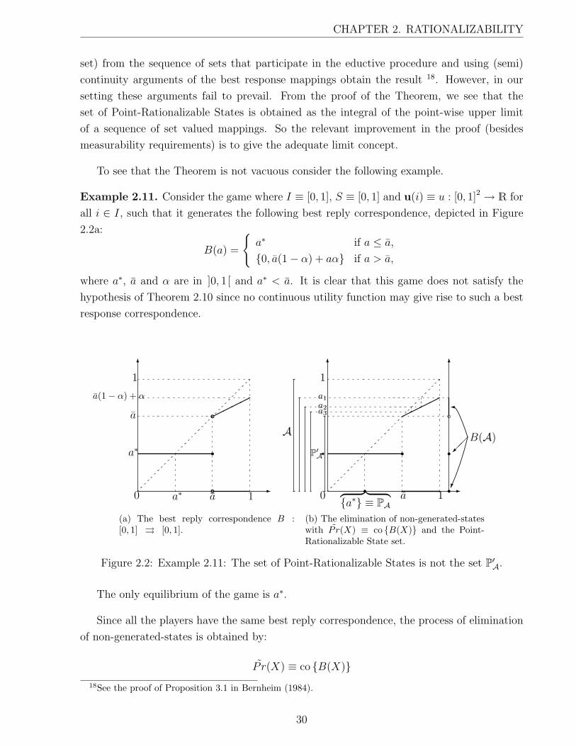
CHAPTER 2. RATIONALIZABILITY
set) from the sequence of sets that participate in the eductive procedure and using (semi)
continuity arguments of the best response mappings obtain the result 18. However, in our
setting these arguments fail to prevail. From the proof of the Theorem, we see that the
set of Point-Rationalizable States is obtained as the integral of the point-wise upper limit
of a sequence of set valued mappings. So the relevant improvement in the proof (besides
measurability requirements) is to give the adequate limit concept.
To see that the Theorem is not vacuous consider the following example.
Example 2.11. Consider the game where I ≡ [0, 1], S ≡ [0, 1] and u(i) ≡ u : [0, 1]2 → R for
all i ∈ I, such that it generates the following best reply correspondence, depicted in Figure
2.2a:
B(a) =
{a∗ if a ≤ a,
{0, a(1− α) + aα} if a > a,
where a∗, a and α are in ]0, 1[ and a∗ < a. It is clear that this game does not satisfy the
hypothesis of Theorem 2.10 since no continuous utility function may give rise to such a best
response correspondence.
6
-aa∗ 1
a(1− α) + α
1
a
a∗
0
rb
����b
(a) The best reply correspondence B :[0, 1] ⇒ [0, 1].
-
6 6
�P′A
a3a2
a1
A
a︷ ︸︸ ︷{a∗} ≡ PA
1
10
.......... ....................
................
....................
........................
............................
�
��
.
...........................................
............................................
.............................................
..............................................
B(A)rrr
br����
(b) The elimination of non-generated-stateswith P r(X) ≡ co {B(X)} and the Point-Rationalizable State set.
Figure 2.2: Example 2.11: The set of Point-Rationalizable States is not the set P′A.
The only equilibrium of the game is a∗.
Since all the players have the same best reply correspondence, the process of elimination
of non-generated-states is obtained by:
P r(X) ≡ co {B(X)}18See the proof of Proposition 3.1 in Bernheim (1984).
30
CHAPTER 2. RATIONALIZABILITY
The image through the best reply correspondence of the state set is
B(A) ≡ {0, a∗} ∪ ]a, a(1− α) + α ] ,
then P r(A) ≡ co {B(A)} ≡ [0, a(1− α) + α].
Then the second iteration is obtained by
P r2(A) ≡ co
{B(P r(A)
)}≡ co {B([0, a(1− α) + α])}
≡ co {{0, a∗} ∪ ]a, a(1− α) + α(a(1− α) + α) ]}≡[0, a(1− α2
)+ α2
].
We see from the form of the best reply correspondence that on each iteration of P r we get
an interval of the form [0, at] where the sequence {at}+∞t=0 satisfies:
at+1 = a(1− α) + atα,
which gives, for t ≥ 1,
at = a(1− αt
)+ αt,
with a0 = 1, and so the sequence is decreasing and converges to a (see Figure 2.2b). This
allows for us to see that P′A ≡ [0, a]. However,
P r(P′A) ≡ co {B(P′A)} ≡ co {B([0, a])} ≡ co {{a∗}} ≡ {a∗} P′A.
and so P′A is not equal to PA, which is in fact equal to the set of equilibria: the singleton {a∗}.
Theorem 2.4 implies that if the set of Point-Rationalizable Strategies (or States for what
it matters) is well defined, then it is not empty, since as we already said, all the equilibria
belong to this set. From Theorem 2.10 we get as a Corollary that in the games that we are
considering, the set of Point-Rationalizable States is well behaved.
Corollary 2.12. The set of Point-Rationalizable States of a game u is well defined, non-
empty, convex and compact.
Proof.
From Theorem 2.10, PA is the intersection of a nested family of non-empty compact
31
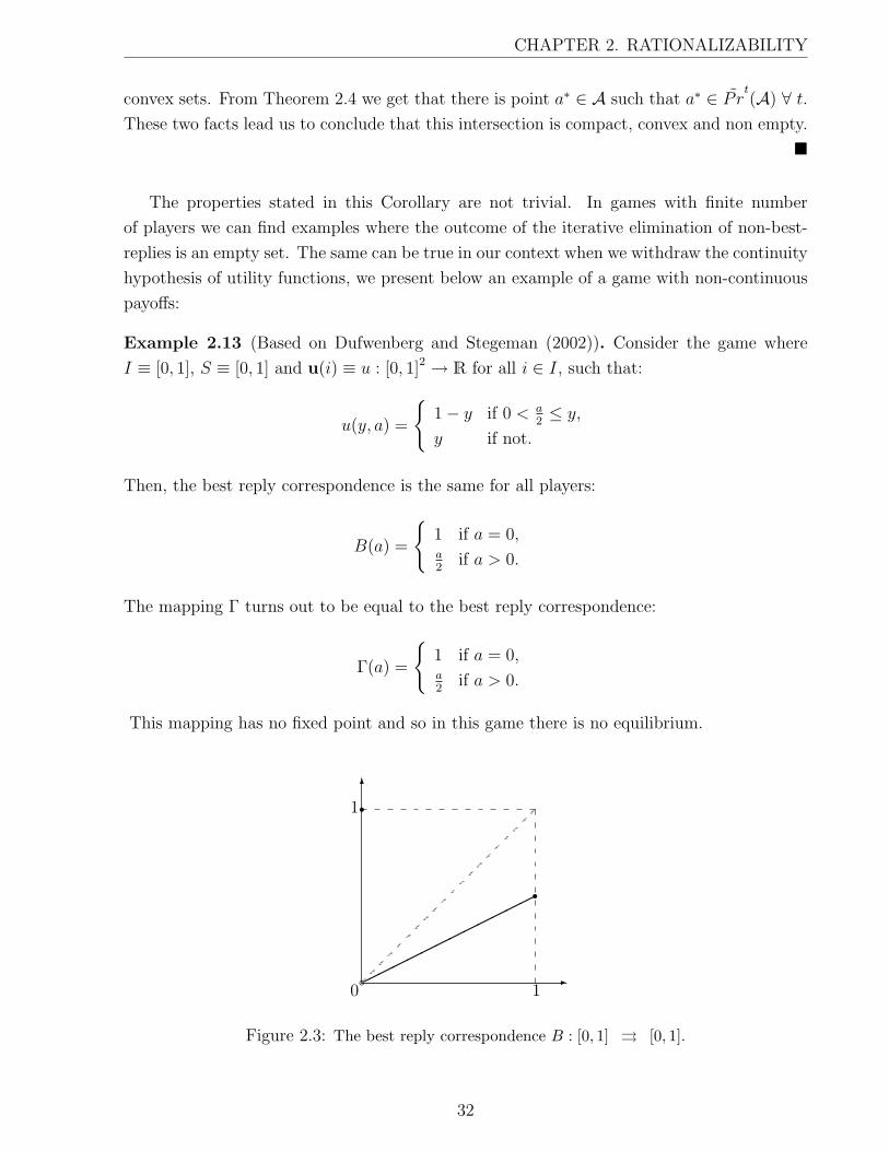
CHAPTER 2. RATIONALIZABILITY
convex sets. From Theorem 2.4 we get that there is point a∗ ∈ A such that a∗ ∈ P rt(A) ∀ t.These two facts lead us to conclude that this intersection is compact, convex and non empty.
�
The properties stated in this Corollary are not trivial. In games with finite number
of players we can find examples where the outcome of the iterative elimination of non-best-
replies is an empty set. The same can be true in our context when we withdraw the continuity
hypothesis of utility functions, we present below an example of a game with non-continuous
payoffs:
Example 2.13 (Based on Dufwenberg and Stegeman (2002)). Consider the game where
I ≡ [0, 1], S ≡ [0, 1] and u(i) ≡ u : [0, 1]2 → R for all i ∈ I, such that:
u(y, a) =
{1− y if 0 < a
2≤ y,
y if not.
Then, the best reply correspondence is the same for all players:
B(a) =
{1 if a = 0,a2
if a > 0.
The mapping Γ turns out to be equal to the best reply correspondence:
Γ(a) =
{1 if a = 0,a2
if a > 0.
This mapping has no fixed point and so in this game there is no equilibrium.
6
-
r
b
r
1
10������������
Figure 2.3: The best reply correspondence B : [0, 1] ⇒ [0, 1].
32

CHAPTER 2. RATIONALIZABILITY
Let us study the Point-Rationalizable States set. The image through the best reply
correspondence of the state set is B(A) ≡ {1} ∪ ]0, 1/2], then
P r(A) ≡ co {B(A)} ≡ ]0, 1] ,
the second iteration gives
P r2(A) ≡ co
{B(P r(A)
)}≡ co {B( ]0, 1])} ≡ ]0, 1/2]
and the third
P r3(A) ≡ co
{B(P r
2(A))}≡ co {B( ]0, 1/2])} ≡ ]0, 1/4] , . . . , etc..
Then the set P′A ≡ ∅ and so PA ≡ ∅, that is, in this example there is no set X ⊆ A that
satisfies X ⊆ P r(X).
Although Theorem 2.10 and Corollary 2.12 assure that the eductive procedure achieves
a non-empty Point-Rationalizable set of states, we see from Examples 2.11 and 2.13 that
even in cases where the eductive procedure fails, in the sense that it does not deliver the
Point-Rationalizable set, we may still identify a set as the correct Point-Rationalizable State
set following our Definition 2.7 (in Example 2.11 the set PA is the singleton that contains
the equilibrium and in Example 2.13 it is the empty set). Even more, the eductive procedure
can (obviously) help to locate such set even in the case of failure and emptiness. The
original motivation to introduce rationalizability in economic contexts is the plausibility of the
Rational Expectations Hypothesis. In consequence we allow an empty (Point-)Rationalizable
set, under the definition of rationalizability, interpreting such as a pessimistic answer to the
possibility of the coordination of expectations.
Another property stated in Corollary 2.12 and an important consequence of Theorem
2.10, is the convexity of the Point-Rationalizable States set, since in the case where we have
multiple equilibria in the set of states, we know that the convex hull of this set of equilibria is
also contained in the set of Point-Rationalizable States. This inclusion may be strict since if
we have multiple equilibria in the set of strategies, even with uniqueness in the set of states,
we may have multiple Point-Rationalizable States 19. Convexity of the Point-Rationalizable
States set is a relevant property since it has not been obtained (to our knowledge) for any
other concept related to Rationalizability.
19See Proposition 2.17.
33

CHAPTER 2. RATIONALIZABILITY
3.3 Point-Rationalizable Strategies vs. Point-Rationalizable States
It is straightforward to ask how the concepts that we just defined are related. To address
this issue, note that for the class of non-atomic games that we are considering, the iterations
of the strategy-elimination and state-elimination mappings (Pr and P r) are equivalent in the
following sense. Consider the set to set mappings A and B defined below. Let A : P(SI)→
P(A) be defined by:
A(H) :=
a ∈ A :a =
∫I
s(i) di and s is a measur-
able function in H
≡ A(H)
and let B : P(A)→ P(SI)
be:
B(X) :=
{s ∈ SI :
s is a measurable selection of
i ⇒ B(i,X)
}.
These mappings satisfy
X1 ⊆ X2 ⊆ A =⇒ B(X1) ⊆ B(X2)
H1 ⊆ H2 ⊆ SI =⇒ A(H1) ⊆ A(H2) .(2.9)
Then, in the context of a game u, the mappings Pr and P r satisfy:
Pr(H) ≡ B(A(H)
)P r(X) ≡ A
(B(X)
) (2.10)
In particular, we get,
P r0(A) ≡ A ≡ co {S} ≡ A
(SI)
which implies by induction that:
P rt(A) ≡ A
(Prt(SI))
Prt(SI)≡ B
(P r
t−1(A))
34
CHAPTER 2. RATIONALIZABILITY
Theorem 2.14. In a game u we have:
PS ≡ B(PA) and PA ≡ A(PS) .
Proof.
Note that from (2.10) we have
Pr(B(PA)
)≡ B
(P r(PA)
)≡ B(PA)
P r(A(PS)
)≡ A(Pr(PS)) ≡ A(PS)
That is, the sets B(PA) ⊆ SI and A(PS) ⊆ A satisfy conditions (2.5) and (2.13) respectively,
which implies that B(PA) ⊆ PS and A(PS) ⊆ PA. Then
PS ≡ Pr(PS) ≡ B(A(PS)
)⊆ B(PA) ⊆ PS.
The second equality comes from (2.10) while the first inclusion comes from (2.9) and the
previous observation. The proof for the second statement is analogous.
�
We see from Theorem 2.14 that in the context that we are considering, the set of Point-
Rationalizable Strategies is paired with the set of Point-Rationalizable States. This implies
that in the models that interest us, it is equivalent to study Point-Rationalizability in terms
of strategies or states, an intuition claimed by Guesnerie and, of course, present in Example
2.3.
Theorems 2.14 and 2.10 together imply that the set of Point-Rationalizable Strategies PScan be actually computed, in this setting, as the limit of the strategy elimination process
governed by Pr (see condition (2.4)) answering a question that remained unanswered. In
consequence, we have that in a game u we can obtain the sets of Point-Rationalizable States
and Strategies through the eductive process in the respective set (A or SI).
Corollary 2.15. Let us write P′S :=⋂∞t=0 Pr
t(SI). The set of Point-Rationalizable Strategy
Profiles of a game u can be calculated as
PS ≡ P′S
≡∞⋂t=0
Prt(SI)
35

CHAPTER 2. RATIONALIZABILITY
3.4 Strongly Point Rational Equilibrium
As we have already said, Guesnerie defines the concept of (local) Strongly Rational Equi-
librium as an equilibrium that is the only Rationalizable State of an economic system. A
particular feature of the work therein developed is that although the definition of Rationaliz-
ability is stressed in terms of strategy profiles, that is, on the profile of individual production
quantities, the study of the (local) stability of the (unique) equilibrium can be developed in
terms of aggregate production or even prices (see note 13). In our context, Strong Rationality
would be defined in terms of the aggregate variable a ∈ A.
Our purpose in this section then is to explore the relation between strategy profiles and
aggregate states when we are interested in Strong Rationality and Point-Rationalizability.
Definition 2.16. An equilibrium state a∗ ∈ A is a Strongly Point Rational Equilibrium if
PA = {a∗}.
Note that if a state a∗ satisfies PA = {a∗}, then it is the unique equilibrium of the system
since (i) all equilibria are in PA and (ii) P r({a∗}) ≡ {a∗} implies that a∗ is the unique
value obtained from the integral of the best response mapping i ⇒ B(i, a∗) and so is an
equilibrium. Analogously if PS ≡ {s∗}, then s∗ is the unique Nash Equilibrium of the game,
since all Nash Equilibria are in PS and Pr({s∗}) ≡ {s∗} implies that s∗ is the (unique)
measurable selection of i ⇒ Br(i, s∗) and so it is a Nash Equilibrium. In particular this
says that Br(i, s∗) is λ-a.e. single valued and hence can be associated to the concept of strict
Nash Equilibrium.20
Proposition 2.17. If s∗ is a Nash Equilibrium of u and∫Is∗ = a∗, then:
a∗ is Strongly Point Rational =⇒ PS ≡
s ∈ SI :
s is a measur-
able selection of
i ⇒ B(i, a∗)
PS ≡ {s∗} =⇒ a∗ is Strongly Point Rational
In particular, if B(i, · ) is single valued at a∗ λ-a.e. on I, then,
a∗ is Strongly Point Rational ⇐⇒ PS ≡ {s∗}
Proof.
20A situation in which any unilateral deviation incurs in a loss.
36

CHAPTER 2. RATIONALIZABILITY
By the definition of PA and PS and the property of PA stated in Theorem 2.14 we have,
B(PA) ≡ PS (2.11)
Suppose that PS ≡ {s∗}. Then, a∗ is an equilibrium, so it satisfies a∗ ∈ PA which in turn
implies that PA 6= ∅. Property (2.11) gives
PS ≡ {s∗} =⇒ P r(PA) ≡ {a∗}
and by the definition of PA,
PA ≡ P r(PA) .
For the proof in the opposite sense, analogously we get:
A(PS) ≡ PA (2.12)
Since s∗ is a Nash Equilibrium, PS 6= ∅ and then from (2.12) we get:
PA = {a∗} =⇒ Pr(PS) ≡
s ∈ SI :
s is a measur-
able selection of
i ⇒ B(i, a∗)
And from the definition of PS,
PS ≡ Pr(PS)
�
Proposition 2.17 shows that it is possible to study Eductive Stability of models with
continuum of agents that fit our framework using the set of states as well as the set of strate-
gies. Moreover, it can be even desirable to use the former approach since (local) uniqueness
and stability are more pertinent in terms of the state of the system rather than in terms of
strategy profiles, as is discussed in the previous section. For instance, the study of Strategic
Complementarities in coordination games or Strategic Substituability in general models as
well, can be undertaken by looking at states of the system rather than strategy profiles (see
the books by Cooper (1999) and Chamley (2004). See as well Guesnerie (2005) and Guesnerie
and Jara-Moroni (2007)).
37

CHAPTER 2. RATIONALIZABILITY
4 Rationalizability vs Point-Rationalizability
Rationalizability differs from Point-Rationalizability on the way we address forecasts.
For Rationalizability, forecasts are no longer points in the corresponding sets but probabil-
ity distributions whose supports are contained in these sets. Then, when a player has a
subjective probability forecast over what may occur with the rest of the economic system,
he maximizes his expected utility with respect to such a probability distribution to make a
decision. Rationality implies that players should not give positive weight in their forecasts
to strategies that are not best response to some rationally generated forecast.
Rationalizable Strategy Profiles, for instance, should be obtained from a similar exercise
as done in Subsection 3.1, but considering forecasts as probability measures over the set
of strategies of the opponents. Loosely speaking, each player should consider a profile of
probability measures (his subjective forecasts over each of his opponents’ play) and maximize
some expected utility, expectation taken over an induced probability measure over the set of
strategy profiles.
A difficulty in a context with continuum of players, relates with the continuity or measur-
ability properties that must be attributed to subjective beliefs, as a function of the player’s
name. There is no straightforward solution in any case. However, in our framework it is
possible to bypass this difficulty. Using the intuition just described for the strategy profiles
case, we will reformulate the processes of elimination of strategies and states described by
equations (2.3) and (2.6) by considering procedures where players eliminate strategies that
are not best response to any possible (subjective probability) forecast (profile) over a given
set of states or strategy profiles.
We present first, in the next Subsection, the concept of Rationalizable States, where
forecasts and the process of elimination are taken over the set of statesA. Then, in Subsection
4.4 we will make use of Schmeidler’s original framework of games with continuum of players,
to formalize the idea of Rationalizable Strategy Profiles in that context.
4.1 Forecasts over the set of states
Before we enter into context we need to introduce some concepts and some notation. for a
Borel set X ⊆ Rn we denote by P(X) the set of probability measures on the Borel subsets of
X. Equivalently this is the set of probability measures on the Borel sets of Rn whose support
38

CHAPTER 2. RATIONALIZABILITY
is in X. We will endow the set P(X) with the weak* topology w∗ = σ(P(X) , Cb(X)) 21.
For a Borel subset Z of X in Rn, P(Z) can be considered to be a subset of P(X) and the
weak* topology on P(Z) is the relativization of the weak* topology on P(X) to P(Z). The
set X can be topologically identified with a subspace of P(X) by the embedding x 7→ δx.
An important property that we will use is that X is compact if and only if P(X) is compact
(and metrizable, since we use the norm in Rn) 22.
As we said before, in the setting of Rath there is a simple way to get through the inconve-
nience of defining an induced probability measure over the set of strategy profiles, using the
presence of the state variable of the game over which players have an infinitesimal influence.
We consider then games with an aggregate state. In this setting, we again consider players
as having forecasts over the set of states rather than over each of the individual strategy sets.
That is, forecasts are probability measures over the set of states rather than profiles of
probabilities over the set of strategies. We define then for each player the set valued mapping
that gives the actions that maximize expected utility given a probability measure µ over the
set of states A, µ ∈ P(A), B(i, · ) : P(A) ⇒ S:
B(i, µ) : = argmaxy∈S Eµ [u(i, y, a)]
≡ argmaxy∈S
∫Au(i, y, a) dµ(a) .
As it has been along all this document, we can describe then, using B(i, · ), the process
of elimination of unreasonable states, considering that players could now use probability
forecasts over the set of states. If it is common knowledge that the actual state is restricted to
a subset X ⊆ A then players will use strategies only in the set B(i,P(X)) := ∪µ∈P(X)B(i, µ).
This is, each player i ∈ I will behave optimally with respect to some subjective belief about
the outcome of the game, whose support is contained in X. This means that rational strategy
profiles have to be selections of the correspondence i ⇒ B(i,P(X)) that maps the set of
players on their set of optimal responses with respect to any possible forecast over X. The
state of the game will then be the integral of one of these selections. This process is described
with the mapping R : B(A)→ P(A):
R(X) :=
{∫I
s(i) di :s ∈ SI , s is a measurable selection
of i ⇒ B(i,P(X))
}.
≡∫I
B(i,P(X)) di
The set R(X) gives the set of states that are obtained as consequence of optimal behavior
21Recall that Cb(X) is the space of real valued bounded continuous functions on X.22See Aliprantis and Border (1999) for detailed treatments of these and other results.
39

CHAPTER 2. RATIONALIZABILITY
when common knowledge about the outcome of the game is represented by X. As we said
before, the difference between P r and R is that the second process considers expected utility
maximizers. For a given Borel set X ⊆ A, X can be embedded into P(X). This means that
B(i,X) ⊆ B(i,P(X)) and so we have that P r(X) ⊆ R(X).
Proposition 2.18. In a game u, if X ⊆ A is nonempty and closed, then R(X) is nonempty,
convex and closed.
For the proof we will make use of the following Lemma:
Lemma 2.19. Let Y and X be compact subsets of Rn. Given a function u ∈ Cb(Y ×X),
the function U : Y × P(X)→ R, which to each (y, µ) ∈ Y × P(X) associates the expectation
U(y, µ) ≡∫X
u(y, x) dµ(x) ,
is continuous when P(X) is endowed with the weak* topology.
Proof.
We write U as the composition of two functions:
(y, µ) ∈ Y × P(X) → (u(y, · ) , µ) ∈ Cb(X)× P(X)
and (f, µ) ∈ Cb(X)× P(X) →∫X
f(x) dµ(x)
If we endow Cb(X) with the sup norm topology and P(X) with the weak* topology, from
Corollary 15.7 in Aliprantis and Border (1999) we get that (f, µ) →∫fdµ is continuous on
Cb(X)× P(X).
Therefore, the result will follow from the continuity of the function
(y, µ)→ F(y, µ) =(u(y, · ) , µ) .
Note first that this function is defined component to component by functions that depend
each only on one variable, this is F(y, µ) =(F1(y) ,F2(µ)), and second that F2 is the identity.
Thus, we only need to prove that F1 : Y → Cb(X) is continuous for the sup norm topology
in Cb(X).
Let yν → y and take ε > 0.
Since Y ×X is compact and u is in Cb(Y ×X), this function is as well uniformly contin-
40

CHAPTER 2. RATIONALIZABILITY
uous. Thus, ∃ δ > 0 (that depends only on ε) such that
‖ (y, x)−(y′, x′)‖ < δ =⇒ |u(y, x)− u(y′, x′)| < ε
3
Since X is compact ∃ {x1, . . . , xN} ⊂ X such that X ⊆ ∪Ni=1B(xi, δ). This is, for any
x ∈ X there exists xi in the previous set such that x ∈ B(xi, δ).
Finally, since yν → y, there exist for each xi numbers νi such that
‖ (yν , xi)−(y, xi)‖ < δ
for all ν ≥ νi.
All together gives, for ν ≥ max {νi : i ∈ {1, . . . , N}} and x ∈ X:
|u(yν , x)− u(y, x)| < |u(yν , x)− u(yν , xi)|+|u(yν , xi)− u(y, xi)|+|u(y, xi)− u(y, x)|
<ε
3+ε
3+ε
3= ε.
We conclude that u(yν , · ) converges to u(y, · ) for the sup norm topology, which completes
the proof.
�
Proof of Proposition 2.18.
From our assumptions, u(i) belongs to Cb(S ×A), and S and A are compact sets in Rn,
so Lemma 2.19, along with Berges’ Theorem, imply that for each i ∈ I the correspondence
B(i, · ) : P(A) ⇒ S is upper semi continuous. Since X is closed, it is compact, which gives
that P(X) is a compact subset of P(A) and so the set B(i,P(X)) is closed for every i ∈ I.
From Theorem 4 in Aumann (1965) we get that∫IB(i,P(X)) di is closed.
On the other hand, Lemma 2.6 states that the correspondence i ⇒ B(i,X) is measurable,
which means that it has a measurable selection s. Since B(i,X) ⊆ B(i,P(X)), s is also a
selection of i ⇒ B(i,P(X)). This implies that∫IB(i,P(X)) di is nonempty.
Convexity comes from the fact that R(X) is obtained as an integral of a set valued
mapping.
�
The previous Proposition allows us to define the Eductive Process in this case. As usual
41
CHAPTER 2. RATIONALIZABILITY
then we consider the iterative elimination of non generated states, but now allowing for
probability forecasts of players. The iterative process begins with the whole set of outcomes,
in this case A.
R0(A) := A
Then, on each iteration, the states that are not reached by the process R are eliminated:
Rt+1(A) := R(Rt(A)
).
Recall that since we start the process at A, what we get is a nested family of sets that,
following Proposition 2.18, are nonempty convex and closed. The Eductive Process gives
then the set,
R′A :=∞⋂t=0
Rt(A) .
Theorem 2.20. In a game u, the set R′A is non empty, convex and closed.
Proof.
R′A is the intersections of closed convex sets, so it is convex and closed. Theorem 2.4
assures that R′A is nonempty, since equilibria belong to every set Rt(A).
�
As it was the case before, the assumptions of rationality and common knowledge of
rationality imply that players must take into account that all their opponents construct their
subjective forecasts rationally. This is formalized by asking that the set of Rationalizable
States must be a subset of R′A (analogously to (2.7)), in the sense that states that are
eliminated can not rise with positive probability and hence are not rationalizable. On the
other hand, if a state is rationalizable then it must be an outcome associated to optimal
reactions to forecasts with support in the set of Rationalizable States, this means that the
set of Rationalizable States must satisfy an analogous condition to (2.8). This is, the set of
Rationalizable States RA must satisfy
RA ⊆ R(RA) . (2.13)
Note that if a set satisfies condition (2.13), then it is a subset of the set R′A.
Definition 2.21. The set of Rationalizable States is the maximal subsetX ⊆ A that satisfies:
X ⊆ R(X)
42

CHAPTER 2. RATIONALIZABILITY
and we note it RA.
As we have already said, from the definition of the set of Rationalizable States, we have
RA ⊆ R′A. The following Theorem, analogous of Theorem 2.10, shows that these two sets
are actually the same.
Theorem 2.22. The set of Rationalizable States of a game u can be calculated as
RA ≡ R′A
Proof.
The proof follows the proof of Theorem 2.10. There are some aspects in which attention
must be put.
We will show that:
R(R′A) ≡ R′A
Theorem 2.20 assures that R(R′A) is correctly defined.
Suppose that a ∈ R(R′A). By the definition of R, there exists a measurable selection
s : I → S of i ⇒ B(i,P(R′A)), such that a =∫Is. Since R′A is a Borel set and R′A ⊆ Rt(A),
which are as well Borel sets ∀ t ≥ 0, we have that P(R′A) ⊆ P(Rt(A)
)are well defined and, ∀
t ≥ 0, ∀ i ∈ I, B(i,P(P′A)) ⊆ B(i,P(Rt(A)
)). So s is a selection of i ⇒ B
(i,P(Rt(A)
))and then a ∈ Rt+1(A) ∀ t ≥ 0, which means that a ∈ R′A. This proves that R(R′A) ⊆ R′A.
For the other inclusion, we consider again a sequence of set valued mappings F t : I ⇒ S,
t ≥ 0, whose p-lim sup limit will be again very helpful. Consider then ∀ i ∈ I,
F 0(i) := S
F t(i) := B(i,P(Rt−1(A)
))t ≥ 1
We have now ∀ t ≥ 0,
Rt(A) ≡∫I
F t(i) di.
We know that A ≡∫IF 0 is non empty and compact. From Proposition 2.18 we get that so
are the sets Rt(A) for all t ≥ 1.
From Lemma 2.19, we get that ∀ i ∈ I the mapping B(i, · ) : P(A) ⇒ S is u.s.c.
and, as a consequence, the set B(i,P(X)) is compact for any compact subset X ⊆ A. So the
43
CHAPTER 2. RATIONALIZABILITY
correspondences F t are compact valued. From the proof of Theorem 2.10 we get that they all
have a measurable selection, since for a closed set X, B(i,X) ⊆ B(i,P(X)) and from Lemma
2.6 the mappings i ⇒ B(i,X) are measurable and hence have a measurable selection.
Consider then the set valued mapping F : I ⇒ S defined as the point-wise lim sup of
the sequence F t:
F (i) :=(p-lim supt F
t)(i) ≡ lim sup
tF t(i) .
So now let us take a point a ∈ R′A. That is, a ∈∫IF t for all t ≥ 0. This gives a sequence
of measurable selections {st}t∈N, such that a =∫Ist. From the Lemma proved in Aumann
(1976) we get that a ∈∫IF , since for each i ∈ I the cluster points of {st(i)}t∈N belong to
F (i) and a is the trivial limit of the constant sequence∫
st.
To show that F (i) ⊆ B(i,P(R′A)), we use that the weak* topology in P(A) is metrizable
and the upper semi continuity of B(i, · ) : P(A) ⇒ S to give an argument that follows the
one at the end of the proof of Theorem 2.10.
�
We get directly that,
Proposition 2.23. In a game u we have:
PA ⊆ RA
In Proposition 2.23 it is not possible to obtain the equality in a general context. We give
a sufficient condition in our setting to have it.
Proposition 2.24. If in a game u, we have ∀ µ ∈ P(A):
Eµ [u(i, y, a)] ≡ u(i, y,Eµ [a])
then
PA ≡ RA
Proposition 2.24 says that if the utility functions are affine in the state variable, then
we have that the Point-Rationalizable States set is equal to the set of Rationalizable States.
Below we will see that we do have a general setting where the set of Rationalizable Strategies
is well defined and in which we can get a result of equivalence between Point and standard
Rationalizability in the strategy sets, improving the statement of Proposition 2.23. We
address this issue in Subsection 4.4.
44
CHAPTER 2. RATIONALIZABILITY
Proof.
If Eµ [u(i, y, a)] ≡ u(i, y,Eµ [a]) then
B(i, µ) ≡ B(i,Eµ [a]) ,
which implies that
B(i,P(X)) ≡⋃
µ∈P(X)
B(i,Eµ [a]) .
For a convex set X ⊆ A we have Eµ [a] ∈ X, ∀ µ ∈ P(X).
This implies that under the hypothesis of the Proposition if X is convex,⋃µ∈P(X)
B(i,Eµ [a]) ⊆⋃a∈X
B(i, a)
and consequently
B(i,X) ⊆ B(i,P(X)) ≡⋃
µ∈P(X)
B(i,Eµ [a]) ⊆⋃a∈X
B(i, a) ≡ B(i,X) .
This is, B(i,P(X)) ≡ B(i,X) and so R(X) ≡ P r(X).
Noting that A is convex, we get R(A) ≡ P r(A) which are as well convex. By induction
we get that P rt(A) ≡ Rt(A) ∀ t which gives (using the previous notation)
R′A ≡∞⋂t=0
Rt(A) ≡∞⋂t=0
P rt(A) ≡ P′A (2.14)
where these intersections give closed convex sets.
Finally we get,
R(R′A) ≡ R(P′A) ≡ P r(P′A) ≡ P′A ≡ R′A
which implies that R′A ≡ RA. The first inequality comes from (2.14), the second one is true
because P′A is convex, the third one comes from Theorem 2.10 which states that P′A ≡ PAand the last one comes again from (2.14).
We conclude that RA ≡ R′A ≡ P′A ≡ PA.
45

CHAPTER 2. RATIONALIZABILITY
�
4.2 More of Example 2.3
Let us now illustrate our results and definitions with the example that motivates this
presentation. In this example the strategy set was R+. Without loss of generality we can
assume it to be a compact interval S ≡ [0, qmax], where qmax could be the quantity that makes
the price equal to 0 : qmax := inf {P−1(0)}.
Now we identify the state set. As we have already said, we could choose the state set
to be the set of aggregate production quantities or the set of prices. This depends on the
aggregation operator that we are considering.
Let us consider first A to be the operator that gives aggregate production quantities.
This is, A : SI → R+
A(s) ≡∫I
s(i) di.
The set A is the interval
A ≡{q ∈ R : ∃ s ∈ SI , q =
∫I
s(i) di
}≡ co {[0, qmax]}≡ [0, qmax] .
The payoff function u(i, · , · ) : [0, qmax]× [0, qmax]→ R is then:
u(i, s(i) , Q) ≡ P (Q) s(i)− ci(s(i)) .
If we assume P and ci to be continuous and that the measurability requirement over
the function i → ci( · ) is met (for instance if all the producers have the same cost
function), Theorem 2.10 holds and so we can compute the Point-Rationalizable State
set using the eductive procedure described by the right hand side of (2.7). We get as
well the result of Corollary 2.12 and we know then that this set is a compact interval.
Now suppose that we use a variation, as in footnote 11, of the aggregation operator.
In the same setting we will consider the state set to be the set of prices. This is,
A : SI → R+
A(s) ≡ P
(∫I
s(i) di
).
46

CHAPTER 2. RATIONALIZABILITY
This is not the aggregation operator for which we obtained the results. However, we
will see below that they still hold. The set of states A will be identified with the set:
A ≡ {p ∈ R : ∃ q ∈ [0, qmax] , p = P (q)}≡ P ([0, qmax])
≡ [0, pmax] .
We see that since P is a continuous function that goes from one-dimensional aggregate-
production set R+ to the set of prices [0, pmax] ⊂ R, this set turns out to be convex.
The utility function is now u(i, · , · ) : [0, qmax]× [0, pmax]→ R:
u(i, s(i) , p) ≡ ps(i)− ci(s(i)) .
Continuity of P implies that Theorem 2.10 still holds and so we can compute the
Point-Rationalizable State set using the eductive procedure described by the right hand
side of (2.7) using A instead of the integral. Since the strategy and state sets are
unidimensional23 we get the result of Corollary 2.12 and we know then that this set is
a compact interval.
Furthermore, in this second approach to the example we have that the payoff function
is affine in the state variable and so Proposition 2.24 holds and we then see that what
we are actually calculating is in fact the set of Rationalizable States (Rationalizable
Prices).
The equivalence between Rationalizable and Point-Rationalizable sets for the case of prices is
obtained directly from Proposition 2.24. The question remains on whether this holds for the
first approach. Clearly the payoff function is not necessarily affine on production quantities
and so we can not apply this Proposition directly. However, without making any further
assumptions we do have that the set of Rationalizable and Point-Rationalizable States in
the “ aggregate production quantities” approach are the same. For this, note that we have
already argued that the set of Point-Rationalizable States is an interval in R. Then, since
the model presents strategic substitutes the limits of this interval are actually the largest
and smallest Rationalizable States (Guesnerie and Jara-Moroni 2007). This implies that the
whole interval is the set of Rationalizable States.
23Otherwise we would have it if we had used only the integral and so aggregate production instead ofprices.
47

CHAPTER 2. RATIONALIZABILITY
4.3 Forecasts over the set of strategies
When we consider forecasts over the sets of strategies, players should have a prior over
each of the other player’s individual actions. A forecasts in this case then would be a profile
of probability measures with support in the set of strategies S. The question is not trivial
since what we would have in this case is a continuum of random variables indexed by the set
of players and it is not clear how payoff should depend on this profile of probability measures.
However, in the setting of the original paper by Schmeidler (1973) this technical issue can
be overtaken since in this setting payoffs depend on the profiles of probability measures
that represent mixed strategies, which are the same mathematical objects as forecasts. We
will give first a loose description of how the eductive process should work when agents use
forecasts over the set of strategies, to continue with a formal description for the case where
S is a finite pure strategy set.
Given a set of strategy profiles H ⊆ SI , consider the set of strategies that a player i ∈ Imay use in strategy profiles in H and denote it H(i):
H(i) := { y ∈ S : y = s(i) , and s ∈ H} .
Ideally we would like to have forecasts on this set, and use the set P(H(i)). Since we do not
know whether H(i) is a Borel set, we may use for instance the closure of H(i), cl{H(i)} and
consider then P(cl{H(i)}).
We will say that a (measurable) mapping m : I → P(S) is a forecast profile over H if m(i)
has support on cl{H(i)} λ-a.e.. The question is, how should rational forecasts be generated?
If originally any strategy can be used, when thinking about possible actions taken by their
rivals players should consider any possible forecast profile in the set of actions. This should
generate for each player a set of best-replies-to-forecasts. The issue is still on how players
use their forecasts to generate this set, but suppose we have this. Once all the players have
done this exercise, we will have a correspondence that maps players to the set of strategies
that represents all the possible strategy profiles that could be played reacting optimally to
some forecast (where different players could be using different forecasts, recall that this is an
issue of forecasting the forecasts of the others). This correspondence would be the result of
a first iteration and should be the point of depart for the second iteration. Forecasts now
should be profiles of probability measures where the support of each probability should be
in the closure of the set associated to each player by this correspondence.
We define the mapping of best-reply-to-forecasts as the set of strategies that maximize
48
CHAPTER 2. RATIONALIZABILITY
some “expected” utility given a forecast profile on S, Br(i, · ) : P(S)I ⇒ S:
Br(i,m) := argmaxy∈S EP(m) [π(i, y, s)] .
We use the notation EP(m) to represent that the payoff that is being maximized is an expected
payoff where the expectation comes from the fact that players are using non-degenerate
forecasts over the set of strategies. We note P(m) to indicate that the profile m induces in
some sense a probability measure over the set of strategy profiles. We do not give an answer
here on to how this is done.
Given a measurable set valued mapping F : I ⇒ S, we can obtain, for each agent i ∈ I,
the set of best-replies to forecasts over this mapping as:
Br(i, F ) :=
{y ∈ S :
y ∈ Br(i,m), m is a fore-
cast profile over F
}. (2.15)
Finally, we can define the process of elimination of non best-reply-to-forecasts, described in
the previous paragraphs, with the mapping R that takes a set valued mapping F : I ⇒ S
and returns a subset R(F ) ⊆ SI ,
R(F ) :=
s ∈ SI :
s is a measur-
able selection of
i ⇒ Br(i, F )
. (2.16)
The process24 described by equation (2.16) considers that strategy profiles that are “kept”
are those that can be constructed from best replies of agents taking decisions considering any
of the possible forecast profiles over F . Of course, as was the case before, on a same strategy
profile s of R(F ) the strategies of two different agents can be best-responses to two different
forecast profiles over F .
Definition 2.25. The set of Rationalizable Strategy Profiles is the maximal subset H ⊆ SI
that satisfies:
H ⊆ R(H)
and we note it RS.
For each player, i ∈ I, there will be a set of Rationalizable Strategies, namely the union,
over all the rationalizable strategy profiles in RS, of the best response set of the considered
player. That is, the set of Rationalizable Strategies for player i ∈ I is,
RS(i) := Br(i,RS)
24The set R(F ) can itself be regarded as a set valued mapping from I to S. This has to be taken in accountto have the set of Rationalizable Strategies well defined.
49

CHAPTER 2. RATIONALIZABILITY
So now that we have presented the main ideas of rationalizability in terms of strategies,
let’s turn to a setting where the best-reply-to-forecast mapping has a concrete sense.
4.4 Games with a continuum of players and finite strategy set
In Schmeidler’s formulation of a game with a continuum of players, payoff functions
π(i, · , · ) are defined on the product set ∆ ×∆I , where{e1, · · · , eL
}⊆ RL is a finite set of
pure strategies that we identify with the canonical base of RL and ∆ ≡ co{{e1, · · · , eL
}}is the set of mixed strategies, the convex hull of
{e1, · · · , eL
}and the simplex in RL. The
functions π(i, · , · ) : ∆×∆I → R take in this setting the form:
π(i, y,m) := y · h(i)(m) (2.17)
where h(i) : ∆I → RL is an auxiliary vector utility function whose coordinate l gives the
utility of player i when he chooses action el, m is a (mixed) strategy profile and y ∈ ∆ is
a (mixed) strategy of player i. If payoffs of players depend on the integral of the (mixed)
strategy profile m,∫Im, then we can say that Schmeidler’s setting is ours with S ≡ A ≡ ∆.
In this case the functions h(i) can be regarded as depending only on the values of the integrals
(as in our setting)25. As quoted by Schmeidler himself, the central result of his paper is
the existence and purification theorem, Theorem 2.26 below, where the main assumption is
precisely this last one. We state this theorem in the context of our framework.
Theorem 2.26 (Schmeidler 1973). If the following conditions are satisfied:
1. The functions h(i) depend only on the integral of the mixed strategy profile m,
2. The functions h(i) : ∆→ RL such that h(i)(m) ≡ h(i)(∫
m), are continuous,
3. For all m ∈ ∆I and all l, k ∈ {1, . . . , L} the set{i ∈ I : h(i)l(m) > h(i)k(m)
}is measurable,
then there exists a Pure Strategy Nash Equilibrium of the game π.
This theorem motivates that we look at Schmeidler’s formulation from a slightly different
point of view. As we have already said, one possibility is to consider this setting in the context
25See Rath (1992) for a discussion on this matter.
50
CHAPTER 2. RATIONALIZABILITY
of a game u where the set of strategies, S, is S ≡ ∆. The implicit properties imposed on
payoff functions in this definition imply the hypothesis of Theorem 2.26 and so we know that
the results stated so far are true for the set of mixed strategies. However, if we keep focusing
on the set of pure strategies, we can benefit from the structure of Schmeidler’s formulation
to have a well defined best-reply-to-forecast mapping. The payoff functions depend on the
integral of the mixed strategy profile, in particular when we consider only pure strategies they
also depend on the integral of pure strategy profiles. We can make then a difference between
(Point-)Rationalizability in pure or mixed strategies. At this point we have to introduce
some more notation: we will represent by a subscript on the corresponding set or operator
whether we are considering pure or mixed strategies 26. In Schmeidler’s formulation we have
Sp ≡{e1, · · · , eL
}and Sm ≡ ∆. We continue to consider the game where S ≡ A ≡ ∆ and
so A is the same as the mixed strategy set ∆ which in turn is equal to the set of probability
measures over the set of pure strategies P(Sp), and so we get:
S ≡ Sm ≡ A ≡ ∆ ≡ P({e1, · · · , eL
})≡ P(Sp) .
If Sp is a finite pure strategy set, then any forecast in the form of a probability distribution
over a subset Y ⊆ Sp can be considered as a point in P(Y ) ≡ co {Y } ⊆ ∆ ≡ co {Sp}. So a
forecast profile would be a function m : I → co {Y }. Since mixed strategies are the same
mathematical objects as probability forecasts over the set of actions of each player, in the
current setting we get to identify the expected utility EP(m) [π(i, y, s)] mentioned above, with
the following expression:
EP(m) [π(i, y, s)] ≡ y · h(i)(m)
≡ u
(i, y,
∫m
)(2.18)
Where now EP( · ) [π(i, · , s)] : Sp ×∆I → R is a function that depends on the pure strategy
y ∈ Sp and we interpret the profile of probability distributions m ∈ ∆I ≡ P(S)I as a forecast,
under the hypothesis that h(i) depends on m through the integral.
In this setting then we get that the set of forecast profiles on a mapping F : I ⇒ Sp can
be described by the mapping co {F} : I ⇒ ∆ defined as co {F}(i) := co {F (i)}. With this,
26For instance, the pointwise eductive procedure Pr can be defined on pure strategies:
Prp(H) ≡{
s ∈ SIp :
s is a measurable selection of the corre-spondence i ⇒ Brp(i,H)
}where H ⊆ SI
p and Brp(i, · ) : SIp ⇒ Sp is defined by:
Brp(i, s) ≡ argmax {π(i, y, s) : y ∈ Sp}
51

CHAPTER 2. RATIONALIZABILITY
we can now consider six different rationalizable sets:
1. The set of Point-Rationalizable Pure Strategies PSp
2. The set of Point-Rationalizable Mixed Strategies PSm
3. The set of Rationalizable Pure Strategies RSp
4. The set of Rationalizable Mixed Strategies RSm
5. The set of Point-Rationalizable States PA
6. The set of Rationalizable States RA
Where the first three have been proved to be well defined and can be obtained from the
eductive processes defined by optimal strategies and forecasts on the corresponding sets.
The last two have been discussed with more detail in Subsections 3.2 and 4.1.
Theorem 2.27. In a game u where S ≡ ∆ we have,
∀ t, Prtp(SIp)≡ Rt
p
(SIp).
Proof.
From the relation in (2.18) we can see that to look at all forecast profiles is equivalent
to look at all the integrals of such profiles. Moreover, we see that in equation (2.15), and
considering F to be the constant mapping F (i) ≡ Sp, the set of forecast profiles over F
is the set valued mapping co {F} as defined above. That is, to obtain Brp(i, SIp
)we are
interested in the integral of F while the calculus of Brp(i, F ) considers the integral of co {F}.From Aumann (1965) the integral of the convex hull mapping is equal to the integral of the
mapping itself and so we have: ∫I
F (i) di ≡∫I
co {F}(i) di.
So no matter whether we are considering point or standard forecasts we obtain the same set
of states. In consequence we get that the set of maximizers is the same:
Brp(i, SIp
)≡ Brp(i, F )
Thus we take measurable selections from the same mapping and so,
Prp(SIp)≡ Rp
(SIp).
52
CHAPTER 2. RATIONALIZABILITY
By induction over t we get that
Prtp(SIp)≡ Rt
p
(SIp).
�
Corollary 2.28. In a game u where S ≡ ∆ we have,
RSp ≡ PSp
Corollary 2.28 says that in the setting where payoff functions depend on the integral of the
mixed strategy profile, and we consider S to be the set of mixed strategies associated to a finite
pure strategy set, then we get that Point-Rationalizability is equivalent to Rationalizability
in terms of pure strategy profiles.
In this context we identify the set PS with PSm and so from Theorem 2.14 we know
that PA ≡ A(PSm). What can we say about the relation between PA and the (Point-
)Rationalizable sets in pure strategies? An answer is given in Corollary 2.29.
Corollary 2.29. In a game u where S ≡ ∆ we have,
(i) PA ≡ A(PSm) and PSm ≡ B(PA)
≡
{m ∈ SIm :
m is a measurable selection of
i ⇒ Bm(i,PA)
};
(ii) PA ≡ A(PSp)
and PSp ≡
{s ∈ SIp :
s is a measurable selection of
i ⇒ Bp(i,PA)
}.
Proof.
Item (i) is the exact same result of Theorem 2.14.
Now note that the best response mappings Bp(i, · ) : A ⇒ Sp and Bm(i, · ) : A ⇒ Sm
satisfy for X ⊆ A:
∪a∈XBp(i, a) ⊆ ∪a∈XBm(i, a) ≡ ∪a∈X co {Bp(i, a)} ⊆ co {∪a∈XBp(i, a)} ,
and so we get
P rp(X) ≡∫I
Bp(i,X) di ⊆∫I
Bm(i,X) di ⊆∫I
co {Bp(i,X)} di ≡ P rp(X) ,
where the integral in the middle is P rm(X). Point (ii) of the Corollary is then consequence
of Theorem 2.14.
53

CHAPTER 2. RATIONALIZABILITY
�
This is, in a game u with S ≡ ∆ ≡ Sm we have that the set of Rationalizable Pure
Strategies is equal to the set of Point-Rationalizable Pure Strategies, and these sets are
paired with the set of Point-Rationalizable States which in turn is paired with the set of
Point-Rationalizable Mixed Strategies.
Finally let’s note that the hypothesis of Theorem 2.26 are implied by the assumptions on
u when we consider the set S to be the set of mixed strategies of a finite strategy set game.
Moreover, since we want to deal with rationalizability in terms of pure strategies, it is not
enough to identify S with the finite set of pure strategies, since in that case we would not
be asking that the utility functions depended on the mixed strategy profiles through their
integral which is crucial for our results.
5 Comments and Conclusions
In this work we have formally introduced the concept of Rationalizability for models that
use a continuum of agents. We have proposed a definition for Point-Rationalizable Strate-
gies in the context of general games with a continuum of players, considering the original
characterization for games with finite set of players, compact strategy sets and continuous
utility functions; as the maximal subset of the strategy profiles set that satisfies being a fixed
point of the process of elimination of non-best response strategies. When such models have
the particularity that payoffs depend on other players’ actions through an aggregate variable
that cannot be unilaterally affected, we have defined as well the set of Point-Rationalizable
States. This last setting is an important generalization of several models that explore Ra-
tional Expectations in economics such as models of currency attacks, stag hunts, standard
markets, macroeconomic dynamics and global games.
We have given sufficient conditions that allow the (Point-)Rationalizable sets to be well
defined and characterized. As in the case of finite player games, continuity properties of the
payoff functions are crucial to assure the convergence of the process of elimination of non-best
replies (the eductive process) to the rationalizable set. For the continuum of players case, an
additional measurability assumption must be made on the mapping that associates players
to their payoff functions to be able to have existence of equilibrium. It turns out that this
same assumption is sufficient to assure the integrability of the set valued mapping that is
used in the eductive process and, in consequence, to obtain the constructive characterization
of the different rationalizbale sets introduced throughout the document.
54
CHAPTER 2. RATIONALIZABILITY
The set of Point-Rationalizable Strategies is paired with the set of Point-Rationalizable
States. We have shown that the set of Point-rationalizable States can be obtained, as in the
case of finite player games with (Point-)Rationalizable Strategies, by eliminating unreason-
able states. Moreover, this set is non-empty, convex and compact.
We have seen as well that for the most important application of Rationalizability in
economic models, namely Strong Rationality, it is equivalent in terms of properties and more
desirable in terms of tractability to use the state approach rather than the strategy profile
approach.
To incorporate standard Rationalizability to our framework, we have formally defined
Rationalizable States. We give a similar characterization for this set and we give a sufficient
(but not at all general) condition on payoff functions, in order to have equivalence between
standard and point Rationalizability.
In the particular case where the strategy sets are finite and payoff functions depend
on the integral of the mixed strategy profile, we were able to formally define Rationaliz-
able strategies and we have extended an equivalence result to Rationalizability vs. Point-
Rationalizability in terms of pure strategy profiles, which in turn implies that in this setting
the three concepts: Rationalizable Pure Strategies, Point-Rationalizable Pure Strategies and
Point-Rationalizable States; give the same outcomes.
We have defined a key concept in a unified exploratory framework that encompasses a
variety of economic models. With this, we have a general framework on which we can study
general properties of equilibria such as (local) eductive stability of equilibria and applications
to models with continuum of agents that feature strategic complementarities or substitutes
(Cooper (1999), Chamley (2004), Guesnerie (2005), Guesnerie and Jara-Moroni (2007)).
55
CHAPTER 3
Strategic Complementarities vs
Strategic Substitutabilities
Introductory Notes
In this Chapter we are interested on stability of equilibria. We use the framework pre-
sented in Chapter 2 to define and study the connection between two different stability con-
cepts of rational expectations equilibria: Expectational Stability and Eductive Stability (or
Strong Rationality). The main difference between these two concepts is the assumption of
heterogeneity of expectations of agents for the case of Eductive Stability. This has already
been done in a series of papers by Evans and Guesnerie (1993, 2003, 2005) in a more specific
model with dynamic characteristics in the two most recent papers. In the present work we
stick to the static situation and focus on strategic uncertainty. As Evans and Guesnerie
claim, (local) Eductive Stability implies (local) Expectational Stability,1 However, in general
Eductive Stability is (strictly) more demanding than Expectational Stability. Nevertheless,
Milgrom and Roberts (1990) prove that in a Supermodular (finite player) Game 2 with unique
Nash Equilibrium (NE), then the latter is the unique Rationalizable Strategy profile (it would
be Strongly Rational in our present terminology). In this light, we study (local) stability of
equilibria of our model with a continuum of agents when endowed with the proper struc-
ture related to Strategic Complementarities (the supermodular case of Milgrom and Roberts
(1990)) and Strategic Substitutabilities (the submodular case).
To introduce complementarity and substitutability we need first to give an order structure
to our strategy and aggregate sets. We use some elements of lattice theory that we introduce
1In the Linear model, Local Eductive Stability is equivalent to Local Expectational Stability if agentsare homogeneous Local Eductive Stability is (strictly) more demanding than Expectational Stability whenagents are heterogeneous
2The definition of supermodular game is given in Subsection 5.1
56

CHAPTER 3. STRATEGIC COMPLEMENTARITIES VS SUBSTITUTABILITIES
before entering into context. The results in the second part of the paper (Sections 5 and
further on) paper are presented under the hypothesis of these sets being the product of
compact intervals of R, however, they remain true if we consider the slightly more general
case where they are complete lattices (see the definition below) and they are stated as such.
Lattices
All the following definitions and the consequences of embedding a model with these con-
cepts can be found with more detail in Topkis (1998).
In a partially ordered set3 (E,≥), the interval [x, y] is the set { z ∈ E : x ≤ z ≤ y} 4.
Given a nonempty subset X ⊆ E an upper bound of X is an element x ∈ E such that x ≥ x′,
∀ x′ ∈ X, analogously a lower bound of X is an element x ∈ E such that x ≤ x′, ∀ x′ ∈ X.
If x is an upper bound of X and x ≤ x for any upper bound of X, then x is the supremum of
X and we note it supE X. The infimum of X, is defined analogously and we note it infE X.
The set E is a lattice if for each two element subset {x, y} ⊆ E, the elements supE {x, y} ∈E and infE {x, y} ∈ E. The lattice E is a complete lattice if any nonempty subset X ⊆ E
has a greatest and smallest bound on E, that is supE X ∈ E and infE X ∈ E. A subset X of
E is a sublattice of E if for all x, y ∈ X, supE {x, y} ∈ X and infE {x, y} ∈ X. The sublattice
X is subcomplete if for any nonempty subset X ′ of X, supE {X ′} ∈ X and infE {X ′} ∈ X.
For functions f : E → R, we say that f is supermodular if ∀ x, y ∈ E,
f(x) + f(y) ≤ f(
infE{x, y}
)+ f
(supE{x, y}
)Given two lattices S1 and S2, we say that a function f : S1 × S2 → R has increasing
(decreasing) differences in it’s two arguments if ∀ x ≥ x′ the function f(x, y) − f(x′, y) is
increasing (decreasing) in y. This is ∀ y ≥ y′,
f(x, y)− f(x′, y) ≥ f(x, y′)− f(x′, y′)
for increasing differences and
f(x, y)− f(x′, y) ≤ f(x, y′)− f(x′, y′)
for decreasing differences.
3The pair (E,≥) is a partially ordered set if ≥ is a binary relation on E that is reflexive, transitive andantisymmetric.
4If x � y then [x, y] = ∅.
57
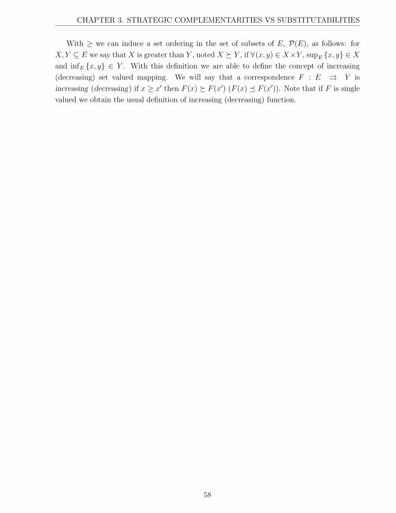
CHAPTER 3. STRATEGIC COMPLEMENTARITIES VS SUBSTITUTABILITIES
With ≥ we can induce a set ordering in the set of subsets of E, P(E), as follows: for
X, Y ⊆ E we say that X is greater than Y , noted X � Y , if ∀(x, y) ∈ X×Y , supE {x, y} ∈ Xand infE {x, y} ∈ Y . With this definition we are able to define the concept of increasing
(decreasing) set valued mapping. We will say that a correspondence F : E ⇒ Y is
increasing (decreasing) if x ≥ x′ then F (x) � F (x′) (F (x) � F (x′)). Note that if F is single
valued we obtain the usual definition of increasing (decreasing) function.
58

CHAPTER 3. STRATEGIC COMPLEMENTARITIES VS SUBSTITUTABILITIES
Full Paper. Current version: Guesnerie and Jara-Moroni (2007)
Expectational Coordination in a class of
Economic Models : Strategic Substitutabilities
versus Strategic Complementarities
Abstract
We consider an economic model that features : 1. a continuum of agents 2. an
aggregate state of the world over which agents have an infinitesimal influence. We
first propose a review, based on work by Jara-Moroni (2008b), of the connections
between the eductive viewpoint that puts emphasis on Strongly Rational Expec-
tations equilibrium and the standard game-theoretical rationalizability concepts.
We explore the scope and limits of this connection depending on whether stan-
dard rationalizability versus point-rationalizability, or the local versus the global
viewpoint, are concerned. In particular, we define and characterize the set of
Point-Rationalizable States and prove its convexity. Also, we clarify the role of
the heterogeneity of beliefs in general contexts of expectational coordination (see
Evans and Guesnerie (2005)). Then, as in the case of strategic complementarities
the study of some best response mapping is a key to the analysis, in the case of
unambiguous strategic substitutabilities the study of some second iterate, and of
the corresponding two-period cycles, allows to describe the point-rationalizable
states. We provide application in microeconomic and macroeconomic contexts.
1 Introduction
Our purpose in this paper is twofold.
First, we attempt to bring in a similar light, the standard game theoretical viewpoint of
coordination on rationalizable solutions and the related viewpoint adopted in the study of
expectational coordination in economic contexts, as for example in Guesnerie (1992, 2002),
Evans and Guesnerie (1993, 2003, 2005). In this work, as well as in most related work on
expectational coordination in economic contexts, (Morris and Shin (1998), Chamley (1999,
2004)) as well as in the theory of crisis, economic agents are non-atomic, in the sense that
59

CHAPTER 3. STRATEGIC COMPLEMENTARITIES VS SUBSTITUTABILITIES
they are too small to have a significant influence on the economic system, and the eductive
reasoning that governs the evaluation of expectational stability refers to game-theoretical
rationalizability ideas. Our aim of linking the “economic” and the “game-theoretical” views
brings us to adopt the framework of a game with a continuum of agents and aggregators in the
sense used by Rath (1992). Relying in particular on Jara-Moroni (2008b), we show the precise
connections between the game-theoretical concepts of rationalizability, point-rationalizability
and the economic concepts of eductive stability. We stress the convexity properties of the
different sets of rationalizable outcomes that follow, in the continuum game, from Liapounov
like theorems. We establish the connections between the concepts of IE-Stability, the different
concepts of Strong Rationality as well as between their local counterparts that allow to select
locally eductively stable equilibria.
Second, relying on this framework, we focus attention on two classes of economic prob-
lems. In the first one, aggregate strategic complementarities, we reassess and strengthen well
known game-theoretical results concerning equilibria and rationalizable solutions. The second
class of models has, on the contrary, aggregate strategic substitutabilities. All expectational
properties obtained in the strategic complementarity case are shown to have counterparts
here. In particular, the set of Rationalizable states is precisely located from cycles of order
2 associated with the system. With differentiability assumptions we get stronger results and
simple sufficient conditions assuring the existence of a global Strongly Rational Expectations
or a unique rationalizable solution. Applications are given for example using the general
equilibrium model of Guesnerie (2001).
The paper proceeds as follows. In Section 2, we introduce games with a continuum of
players and we relate it to a class of economic models with a continuum of agents. We show
how this setting may be viewed from a game theoretical point of view and we introduce the
concepts of Economic equilibrium and Nash Equilibrium. In section 3 we formulate Rational-
izability in this context. We introduce first the concepts of Point-Rationalizable Strategies.
We present an economic version of Rationalizability introducing Point-Rationalizable States
and Rationalizable States and we relate these concepts to the game theoretical ones. In
section 4 we address the economic concepts of Iterative Expectational Stability and Educ-
tive Stability using the tools defined in section 3. Then in Section 5 we successively focus
attention on aggregate models with Strategic Complementarities or Strategic Substitutabil-
ities. Our general results here are tightened when we examine the differentiable version of
the model. In Section 7 we conclude.
60

CHAPTER 3. STRATEGIC COMPLEMENTARITIES VS SUBSTITUTABILITIES
2 The canonical model and concepts.
This Section aims at making a careful connection between the underlying game theoret-
ical concepts and the economic application which they are solicited for. We present first a
game theoretical framework that underlies the standard economic model with a continuum
of agents, presented afterwards. We then introduce and compare the parallel tools used for
the analysis.
2.1 Games with a continuum of players
We consider a game with a continuum of players. Non atomic games with continuum of
players where first introduced by Schmeidler (1973). In these games the set of players is the
measure space (I, I, λ), where I is the unit interval of R, I ≡ [0, 1], and λ is the lebesgue
measure. Each player chooses a strategy s(i) ∈ S(i) and we take S(i) ⊆ Rn. Strategy
profiles in this setting are identified with integrable selections5 of the set valued6 mapping
i ⇒ S(i). For simplicity, we will assume that all the players have the same compact strategy
set S(i) ≡ S ⊂ Rn+. As a consequence, since S is compact, the set of meaningful strategy
profiles is the set of measurable functions from I to S 7 noted from now on SI .
In a game, players have payoff functions that depend on their own strategy and the
complete profile of strategies of the player π(i, · , · ) : S × SI → R. In our particular
framework these functions depend, for each player, on his own strategy and an average of the
strategies of all the other players. To obtain this average we use the integral of the strategy
profile,∫Is(i) di. This implies that all the relevant information about the actions of the
opponents is summarized by the values of the integrals, which are points in the set 8
A ≡∫I
S(i) di.
Hypothesis over the correspondence i ⇒ S(i) that assure that the set A is well defined can
be found in Aumann (1965) or in Chapter 14 of Rockafellar and Wets (1998). In this case
5A selection is a function s : I → Rn such that s(i) ∈ S(i).6We use the notation ⇒ for set valued mappings (also referred to as correspondences), and → for
functions.7Equivalently, the set of measurable selections of the constant set valued mapping i ⇒ S.8Following Aumann (1965) we define for a correspondence F : I ⇒ Rn its’ integral,
∫IF (i) di, as:∫
I
F (i) di :={x ∈ Rn : x =
∫I
f(i) di and f is an integrable selection of F}
61

CHAPTER 3. STRATEGIC COMPLEMENTARITIES VS SUBSTITUTABILITIES
we get that A is a convex set (Aumann 1965). Moreover, since S(i) ≡ S we have that 9
A ≡ co {S} . (3.1)
Pay-offs π(i, · , · ) in this setting are evaluated from an auxiliary utility function u(i, · , · ) :
S × co {S} → R such that:
π(i, y, s) ≡ u
(i, y,
∫I
s(i) di
)(3.2)
We assume:
C : For all agent i ∈ I, u(i, · , · ) is continuous.
HM : The mapping that associates to each agent a utility function 10 is measurable.
C is standard and does not deserve special comments. HM is technical but in a sense natural
in this setting. Adopting both assumptions on utility functions put us in the framework of
Rath (1992). We begin by giving a definition of Nash Equilibrium in this setting.
Definition 3.1. A (pure strategy) Nash Equilibrium of a game is a strategy profile s∗ ∈ SI
such that:
∀ y ∈ S, u
(i, s∗(i) ,
∫s∗(i) di
)≥ u
(i, y,
∫s∗(i) di
), ∀ i ∈ I λ-a.e. (3.3)
It is useful to use the best reply correspondence Br(i, · ) : SI ⇒ S defined as:
Br(i, s) := argmaxy∈S π(i, y, s) . (3.4)
The correspondence Br(i, · ) describes the optimal response set for player i ∈ I facing a
strategy profile s.
In our setting, and considering the auxiliary function u(i, · , · ), we can define as well the
optimal strategy correspondence B(i, · ) : A ⇒ S as the correspondence which associates
to each point a ∈ A the set:
B(i, a) := argmaxy∈S {u(i, y, a)} . (3.5)
9Where co {X} stands for the convex hull of a set X (see Rath (1992)).10The set of functions for assumption HM is the set of real valued continuous functions defined on S×co {S}
endowed with the sup norm topology.
62
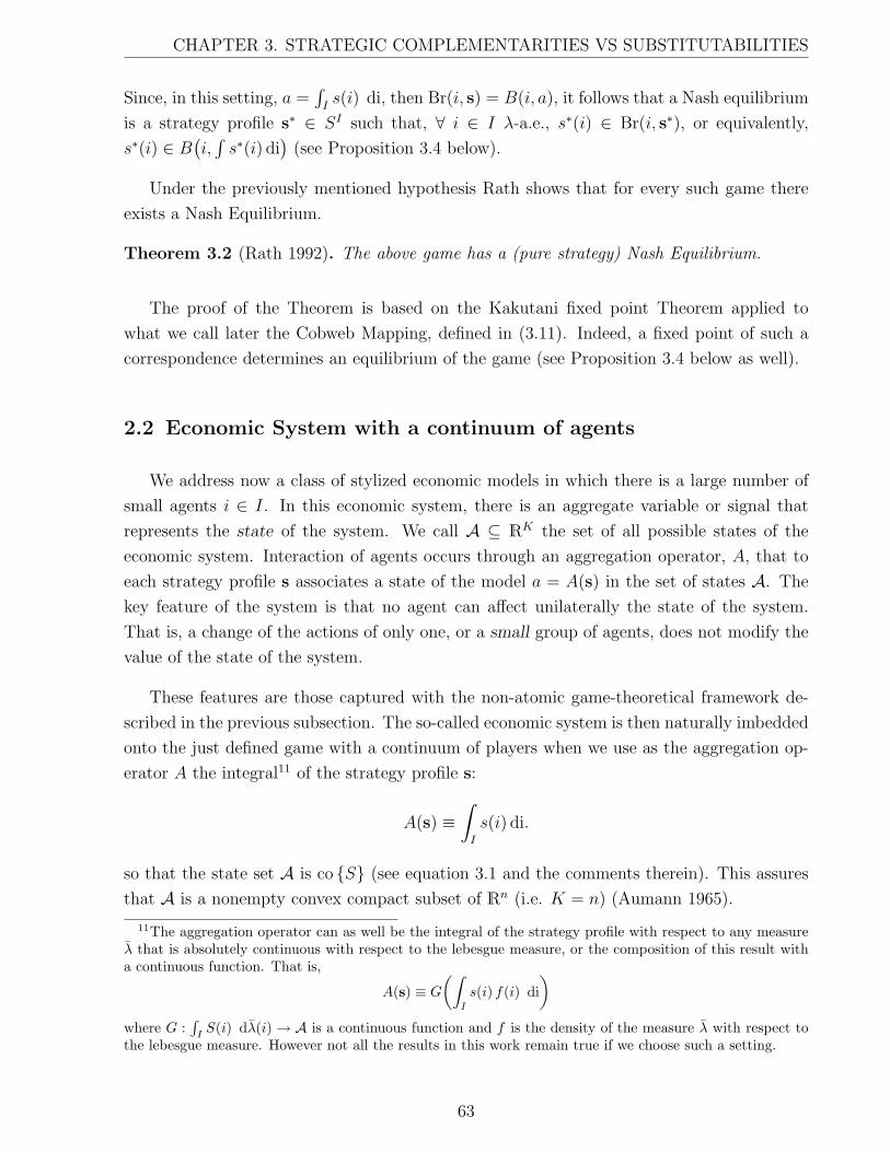
CHAPTER 3. STRATEGIC COMPLEMENTARITIES VS SUBSTITUTABILITIES
Since, in this setting, a =∫Is(i) di, then Br(i, s) = B(i, a), it follows that a Nash equilibrium
is a strategy profile s∗ ∈ SI such that, ∀ i ∈ I λ-a.e., s∗(i) ∈ Br(i, s∗), or equivalently,
s∗(i) ∈ B(i,∫s∗(i) di
)(see Proposition 3.4 below).
Under the previously mentioned hypothesis Rath shows that for every such game there
exists a Nash Equilibrium.
Theorem 3.2 (Rath 1992). The above game has a (pure strategy) Nash Equilibrium.
The proof of the Theorem is based on the Kakutani fixed point Theorem applied to
what we call later the Cobweb Mapping, defined in (3.11). Indeed, a fixed point of such a
correspondence determines an equilibrium of the game (see Proposition 3.4 below as well).
2.2 Economic System with a continuum of agents
We address now a class of stylized economic models in which there is a large number of
small agents i ∈ I. In this economic system, there is an aggregate variable or signal that
represents the state of the system. We call A ⊆ RK the set of all possible states of the
economic system. Interaction of agents occurs through an aggregation operator, A, that to
each strategy profile s associates a state of the model a = A(s) in the set of states A. The
key feature of the system is that no agent can affect unilaterally the state of the system.
That is, a change of the actions of only one, or a small group of agents, does not modify the
value of the state of the system.
These features are those captured with the non-atomic game-theoretical framework de-
scribed in the previous subsection. The so-called economic system is then naturally imbedded
onto the just defined game with a continuum of players when we use as the aggregation op-
erator A the integral11 of the strategy profile s:
A(s) ≡∫I
s(i) di.
so that the state set A is co {S} (see equation 3.1 and the comments therein). This assures
that A is a nonempty convex compact subset of Rn (i.e. K = n) (Aumann 1965).
11The aggregation operator can as well be the integral of the strategy profile with respect to any measureλ that is absolutely continuous with respect to the lebesgue measure, or the composition of this result witha continuous function. That is,
A(s) ≡ G(∫
I
s(i) f(i) di)
where G :∫
IS(i) dλ(i)→ A is a continuous function and f is the density of the measure λ with respect to
the lebesgue measure. However not all the results in this work remain true if we choose such a setting.
63

CHAPTER 3. STRATEGIC COMPLEMENTARITIES VS SUBSTITUTABILITIES
The variable a ∈ A, that represents the state of the system, determines, along with
each agents’ own action, his payoff. For each agent i ∈ I then, we use the payoff function
u(i, · , · ) : S ×A → R introduced in (3.2). Agents act to maximize this payoff function.
In a situation where agents act in ignorance of the actions taken by the others or, for
what matters, of the value of the state of the system, they have to rely on forecasts. That
is, their actions must be a best response to some subjective probability distribution over
the space of aggregate data A. Mathematically, actions have to be elements of the set of
points that maximize expected utility, where the expectation is taken with respect to this
subjective probability. We can consider then the best reply to forecasts correspondence
B(i, · ) : P(A) ⇒ S defined by:
B(i, µ) := argmaxy∈S Eµ [u(i, y, a)] (3.6)
where µ ∈ P(A) and P(A) is the space of probability measures over A. Since the utility
functions are continuous, problems (3.5) and (3.6) are well defined and have always a solution,
so consequently the mappings B(i, · ) and B(i, · ) take non-empty compact values for all
a ∈ A. Clearly B(i, a) ≡ B(i, δa), where δa is the Dirac measure concentrated in a.
An equilibrium of this system is a state a∗ generated by actions of the agents that are
optimal reactions to this state. We denote Γ(a) =∫IB(i, a) di.
Definition 3.3. An equilibrium is a point a∗ ∈ A such that:
a∗ ∈ Γ(a∗) ≡∫I
B(i, a∗) di ≡∫I
B(i, δa∗) di (3.7)
Assumptions C and HM assure that the integrals in Definition 3.3 are well defined 12.
The equilibrium conditions in (3.7) are standard description of self fulfilling forecasts. That
is, in an equilibrium a∗, agents must have a self-fulfilling point forecast (Dirac measures) over
a∗, i.e with the economic terminology, a perfect foresight equilibrium (see Guesnerie (1992)).
It is unsurprising that an equilibrium as defined in (3.7) has as a counterpart in the
game-theoretical approach a Nash Equilibrium of the underlying game as defined in (3.3).
Precisely :
Proposition 3.4. For every (pure strategy) Nash Equilibrium s∗ of the system’s underlying
game, there exists a unique equilibrium a∗ given by a∗ := A(s∗) and if a∗ is an equilibrium of
the system, then ∃ s∗ ∈ SI that is a Nash Equilibrium of the underlying game.
Proof. Indeed, if a∗ satisfies (3.7), then there exists an integrable strategy profile s∗ such that
12This is a consequence of Lemma 2.6 in Chapter 2, which is restated and proved in the appendix of thisChapter as Lemma 3.47, as in the original paper
64

CHAPTER 3. STRATEGIC COMPLEMENTARITIES VS SUBSTITUTABILITIES
s∗(i) ∈ B(i, a∗) and A(s∗) = a∗. That is s∗(i) ∈ B(i,∫Is∗(i) di
), or equivalently
∀ y ∈ S, u
(i, s∗(i) ,
∫s∗(i) di
)≥ u
(i, y,
∫s∗(i) di
), ∀ i ∈ I λ-a.e.
Conversely, if
∀ y ∈ S, u
(i, s∗(i) ,
∫s∗(i) di
)≥ u
(i, y,
∫s∗(i) di
), ∀ i ∈ I λ-a.e. (3.8)
then s∗(i) ∈ Br(i, s) ≡ B(i,∫s∗(i) di
)∀ i ∈ I λ-a.e.. Defining a∗ :=
∫Is∗(i) di we get that
a∗ ∈∫IB(i, a∗) di.
�
We will refer equivalently then, to equilibria as points a∗ ∈ A, representing economic
equilibria, and s∗ ∈ SI , as Nash Equilibria of the underlying game.
Theorem 3.5. The stylized economic model has an equilibrium.
Proof. It is the consequence of the proof of Theorem 3.2 and is related to the previous
Proposition. �
Example 3.6. Variant of Muth’s (1961) model presented in Guesnerie (1992). In this ex-
ample there is a group of farmers indexed by the unit interval. Farmers decide a positive
production quantity q(i) and get as payoff income from sales minus the cost of production:
pq(i) − Ci(q(i)), where p is the price at which the good is sold. The price is obtained from
the inverse demand (or price) function, evaluated in total aggregate production Q. We see
that this model fits our framework.
We already said that the set of agents is the unit interval I = [0, 1] and we endow it with
the lebesgue measure. Strategies are production quantities, so strategy profiles are functions
from the set of agents to the positive line R+ (i.e. n = 1), q : I → R+. The aggregate variable
in this case is aggregate production. Agents can calculate their payoff by knowing aggregate
production through the price function and deciding their production. So the aggregate state
space is the positive line as well, R+ (i.e. K = 1 = n). The payoff of an agent is income
from sales minus cost of production, the utility function is then u(i, q, Q) = P (Q) q − Ci(q).Where P : R+ → R+ is an inverse demand (or price) function that, given a quantity of good,
gives the price at which this quantity is sold. If we suppose that P is bounded and attains
the value 0 from a certain qmax on, then we get that the aggregate state set A is equal to the
set of strategies S(i) ≡ S, and both are the interval [0, qmax]. The aggregation operator, the
integral of the production profile q, gives aggregate production Q =∫Iq(i) di.
65

CHAPTER 3. STRATEGIC COMPLEMENTARITIES VS SUBSTITUTABILITIES
On this example we can make the observation that the state of he game could be chosen
to be the price instead of aggregate production. This is not always the case if we want to
obtain the properties stated further on in this work. However, since this example is one-
dimensional, it is the case that most of the properties herein presented are passed on from
the aggregate production set to the price set.
We are interested now on the plausibility of the equilibrium forecasts, or equivalently to
the assessment of the strength of expectational coordination described here. Our assessment
relies on the concepts of Rationalizability (Bernheim 1984; Pearce 1984) or on the derived
concepts, in our economic framework, of Strong Rationality (Guesnerie 1992). In the next
two sections then, we exploit the game-theoretical viewpoint to asses Rationalizability in the
economic context.
3 Rationalizability and the “eductive learning viewpoint”.
3.1 Rationalizability : the game viewpoint.
Rationalizability is associated with the work of Bernheim (1984) and Pearce (1984). The
set of Rationalizable Strategy profiles were defined and characterized in the context of games
with a finite number of players, continuous utility functions and compact strategy spaces. It
has been argued that Rationalizable strategy profiles are profiles that can not be discarded
as outcomes of the game based on the premises of rationality of players, independence of
decision making and common knowledge (see Tan and da Costa Werlang (1988)).
First, agents only use strategies that are best responses to their forecasts and so strategies
in S that are never best response will never be used; second, agents know that other agents are
rational and so know that the others will not use the strategies that are not best responses
and so each agent may find that some of his remaining strategies may no longer be best
responses, since each agent knows that all agents know, etc. . This process continues ad-
infinitum. The set of Rationalizable solutions is such that it is a fixed point of the elimination
process, and it is the maximal set that has such a property (Basu and Weibull 1991).
Rationalizability has been studied in games with finite number of players. In a game with
a continuum of agents, the analysis has to be adapted. Following Jara-Moroni (2008b), and
coming to our setting, in a game-theoretical perspective, the recursive process of elimination
of non best responses, when agents have point expectations, is associated with the mapping
Pr : P(SI)→ P
(SI)
which to each subset H ⊆ SI associates the set Pr(H) defined by:
Pr(H) :={
s ∈ SI : s is a measurable selection of i ⇒ Br(i,H)}. (3.9)
66

CHAPTER 3. STRATEGIC COMPLEMENTARITIES VS SUBSTITUTABILITIES
The operator Pr represents the process under which we obtain strategy profiles that are
constructed as the reactions of agents to strategy profiles contained in the set H ⊆ SI . If
it is known that the outcome of the game is in a subset H ⊆ SI , with point expectations,
the strategies of agent i ∈ I are restricted to the set Br(i,H) ≡⋃
s∈H Br(i, s) and so actual
strategy profiles must be measurable selections of the set valued mapping i ⇒ Br(i,H). It
has to be kept in mind that strategies of different agents in a strategy profile in Pr(H) can
be the reactions to (possibly) different strategy profiles in H.
We then define :
Definition 3.7. The set of Point-Rationalizable13 Strategy Profiles is the maximal subset
H ⊆ SI that satisfies:
H ≡ Pr(H) . (3.10)
and we note it PS.
Rationalizable Strategies should be obtained from a similar exercise but considering fore-
casts as probability measures over the set of strategies of the opponents. Loosely speaking
each player should consider a profile of probability measures (his forecasts over each of his
opponents play) and maximize some expected utility, expectation taken over an induced prob-
ability measure over the set of strategy profiles. A difficulty in a context with continuum of
players, relates with the continuity or measurability properties that must be attributed to
subjective beliefs, as a function of the agent’s name. There is no straightforward solution in
any case. However, in our framework it is possible to bypass this difficulty. We present in
the next section the concepts of Rationalizable States and Point-Rationalizable States, where
forecasts and the process of elimination are now taken over the set of states A.
3.2 Rationalizability : an “economic” viewpoint.
Before going to the rationalizability, it is useful to describe the Cobweb mapping, which
we will refer to sometimes later as the Iterative Expectational process.
13Following Bernheim (1984) we refer as Point-Rationalizability to the case of forecasts as points in theset of strategies or states and plain Rationalizability to the case of forecasts as probability distributions overthe corresponding set.
67
CHAPTER 3. STRATEGIC COMPLEMENTARITIES VS SUBSTITUTABILITIES
Cobweb Mapping and Equilibrium
Given the optimal strategy correspondence, B(i, · ), defined in (3.5) we can define the
cobweb mapping14 Γ : A ⇒ A:
Γ(a) :=
∫I
B(i, a) di (3.11)
This correspondence represents the actual possible states of the model when all agents react
to the same state a ∈ A. Following Definition 3.3 we see that the equilibria of the economic
system are identified with the fixed points of the cobweb mapping.
Definition 3.8. The set of Aggregate Cobweb Tatonnement Outcomes, CA, is defined by:
CA :=⋂t≥0
Γt(A)
where Γt is the tth iterate15 of the correspondence Γ.
From the proof of Theorem 3.2 (see Rath (1992)) we get that in our framework the cobweb
mapping Γ is upper semi continuous as a set valued mapping, with non-empty, compact and
convex values Γ(a).
State Rationalizability
Below we present the mathematical formulation of Point-Rationalizable States and Ra-
tionalizable States, and explore the relation between Point-Rationalizability and Rationaliz-
ability in our context. We aim at clarifying the different perspectives on equilibrium stability
and the connections between the notions of local and global Strong Rationality (Section
3.2)). For the proofs of the results herein stated and a more detailed treatment the reader is
referred to Jara-Moroni (2008b).
Analogously to what is done in subsection 3.1, given the optimal strategy correspondence
defined in equation (3.5) we can define the process of non reachable or non generated states,
considering forecasts as points in the set of states, as follows:
P r(X) :=
∫I
B(i,X) di (3.12)
14The name cobweb mapping comes from the familiar cobweb tatonnement although in this general contextthe process of iterations of this mapping may not necessarily have a cobweb-like graphic representation.
15This is:Γ0 := A Γt+1 := Γ
(Γt(A)
)
68

CHAPTER 3. STRATEGIC COMPLEMENTARITIES VS SUBSTITUTABILITIES
This is, if initially agents’ common knowledge about the actual state of the model is a subset
X ⊆ A we have that forecasts are constrained by X. Then, if expectations are restricted to
point-expectations, agents deduce that the possible actions of each agent i ∈ I are in the set
B(i,X) :=⋃a∈X B(i, a). Since all agents know this, each agent can only discard the strategy
profiles s ∈ SI that are not a selection of the mappings that assign each agent to the these
sets. Finally, they would conclude that the actual state outcome will be restricted to the set
obtained as the integral of this set valued mapping.
Definition 3.9. The set of Point-Rationalizable States is the maximal subset X ⊆ A that
satisfies the condition:
X ≡ P r(X)
and we note it PA.
We define similarly the set of Rationalizable States. The difference between Rational-
izability and Point-Rationalizability is that in Rationalizability forecasts are no longer con-
strained to points in the set of outcomes. To assess Rationalizability we consider the cor-
respondence B(i, · ) : P(A) ⇒ S defined in (3.6). The process of elimination of non
expected-utility-maximizers is described with the mapping R : B(A)→ P(A):
R(X) :=
∫I
B(i,P(X)) di (3.13)
If it is common knowledge that the actual state is restricted to a borel subset X ⊆ A, then
agents will use strategies only in the set B(i,P(X)) := ∪µ∈P(X)B(i, µ) where P(X) stands
for the set of probability measures whose support is contained in X. Forecasts of agents
can not give positive weight to points that do not belong to X. Strategy profiles then will
be selections of the correspondence i ⇒ B(i,P(X)). The state of the system will be the
integral of one of these selections.
Definition 3.10. The set of Rationalizable States is the maximal subset X ⊆ A that
satisfies:
R(X) ≡ X (3.14)
and we note it RA.
The difference between P r and R is that the second operator considers expected utility
maximizers and so for a given borel set X ⊆ A we have P r(X) ⊆ R(X). We get directly the
result in Proposition 3.13 below.
Bypassing the game-theoretical difficulties occurring in games with a continuum of play-
ers, the states set approach provides a substitute for the Rationalizability concept.
69

CHAPTER 3. STRATEGIC COMPLEMENTARITIES VS SUBSTITUTABILITIES
Rationalizability : the game versus the economic viewpoint
Rationalizability in the context of the games with continuum of players that we are
considering is studied in Jara-Moroni (2008b). Therein it is proved that, in our context,
the set of Point-Rationalizable pure Strategies is paired with the set of Point-Rationalizable
States; moreover, in the context of the original model of Schmeidler16 these sets are also
paired with the set of Rationalizable (pure) Strategies. We state the result that is pertinent
to our framework.
Proposition 3.11. We have:
PS ≡{
s ∈ SI : s is a measurable selection of i ⇒ B(i,PA)}
(3.15)
PA ≡{a ∈ A : a =
∫I
s(i) di and s is a measurable function in PS}. (3.16)
Equations (3.15) and (3.16) stress the equivalence for point-rationalizability between the
state approach and the strategic approach in games with continuum of players : the sets of
point-rationalizable states can be obtained from the set of point-rationalizable strategies and
vice versa. In (3.15) we see that the strategy profiles in PS are profiles of best responses to
PA. Conversely in (3.16) we get that the points in PA are obtained as integrals of the profiles
in PS.
We will make use of Proposition 3.12 below, which provides, in the continuum of agents
framework, a key technical property of the set of Point-Rationalizable States.
Proposition 3.12. The set of Point-Rationalizable States can be computed as
PA ≡∞⋂t=0
P rt(A)
The set PA, indeed obtains as the outcome of the iterative elimination of unreachable
states.
16The functions u(i, · , · ) are defined on a finite strategy set S and depend on the integral of a mixedstrategy profile.
70

CHAPTER 3. STRATEGIC COMPLEMENTARITIES VS SUBSTITUTABILITIES
4 Rationalizable outcomes, Equilibria and Stability
4.1 The global viewpoint.
We denote by E ⊆ A, the set of equilibria of the economic system. The inclusions below
are unsurprising, in the sense that they reflect the decreasing strength of the expectational
coordination hypothesis, when going from equilibria to Aggregate Cournot outcomes, then
to Point-Rationalizable States, and finally to Rationalizable States.
Proposition 3.13. We have:
E ⊆ CA ⊆ PA ⊆ RA
The first inclusion is direct since fixed points of Γ are obtained as integrals of selections
of the best response correspondence i ⇒ B(i, a∗) and so will not be eliminated during the
process that characterizes the set CA. We can obtain the two last inclusions of Proposition
3.13 noting that if a set satisfies X ⊆ P r(X) then it is contained in PA and equivalently if
it satisfies X ⊆ R(X) then it is contained in RA. Then, the second inclusion is obtained
from the fact that each point in CA, as a singleton, satisfies {a∗} ⊆ P r({a∗}) and the third
inclusion is true because the set PA satisfies PA ⊆ R(PA).
An important corollary of Proposition 3.12 is that the set of Point-Rationalizable States
is convex. This is a specific and nice property of our setting with a continuum of agents.
Theorem 3.14.
The set of Point-Rationalizable States is well defined, non-empty, convex and compact.
The set of Rationalizable States is non-empty and convex.
Proof. The properties are obtained from the convexity of each of the sets that are involved
in the intersection in the characterization of PA in Proposition 3.12. That is, PA is the
intersection of a nested family of non-empty, compact, convex sets. Non-emptiness of PA is
guaranteed by Proposition 3.12 along with Theorem 3.2, since an equilibrium would never be
eliminated, and so there exists a point a∗ ∈ A that belongs to every set P rt(A). Proposition
3.13 implies the property for RA, while its’ convexity obtains from the definition.
�
In Evans and Guesnerie (1993), two stability concepts of Rational Expectations Equilibria
are compared: Iterative Expectational Stability, based on the convergence of iterations of
71

CHAPTER 3. STRATEGIC COMPLEMENTARITIES VS SUBSTITUTABILITIES
forecasts; and Strong Rationality, based on the uniqueness of the Rationalizable Outcomes
(Guesnerie 1992) of an economic model. In what follows, we define these two concepts
following the terminology of Guesnerie and Evans and Guesnerie, for our setting.
Definition 3.15. An equilibrium a∗ is said to be Globally Iterative Expectationaly Stable
if ∀ a0 ∈ V any sequence at ∈ Γ(at−1) satisfies limt→∞ at = a∗ (= E).
The terminology of Iterative Expectational Stability is adopted from the literature on
expectational stability in dynamical systems (Evans and Guesnerie (1993, 2003, 2005)). It
captures the idea that virtual coordination processes converge globally, under the implicit
assumption that agents have homogenous deterministic expectations.
Definition 3.16. The equilibrium state a∗ is (globally) Strongly Point Rational if
PA ≡ {a∗} (= E).
The idea is now hat virtual coordination processes converge globally, under the implicit
assumption that agents have heterogenous and deterministic expectations.
Definition 3.17. The equilibrium state a∗ is (globally) Strongly Rational if
RA ≡ {a∗} (= E).
Eductive coordination then obtains when agents have heterogenous and stochastic expec-
tations.
Strong Rationality and Strong Point Rationality can be related to heterogeneous beliefs
of agents. Both concepts refer to heterogenous forecasts of agents, (even if these agents were
homogeneous (have the same utility function)). With Strong rationality, forecasts are based
on stochastic expectations, when with Strong Point Rationalizability, we restrict attention
to point expectations. When we turn to Iterative Expectational Stability (IE-Stability), we
drop the possibility of heterogeneity of forecasts. The iterative process associated with IE-
Stability is based on iterations of the cobweb mapping Γ which describe agents reactions to
the same point forecast over the set of states.
It is straightforward that these concepts are increasingly demanding : Strong Rationality
implies Strong Point Rationalizability that implies Iterative Expectational Stability.
We turn now to the local version of these concepts.
72
CHAPTER 3. STRATEGIC COMPLEMENTARITIES VS SUBSTITUTABILITIES
4.2 The local viewpoint.
We now give the local version of the above stability concepts.
Again, the definition of (local) IE-Stability (Lucas 1978; DeCanio 1979), stated below is
similar to the one given in Evans and Guesnerie (1993)
Definition 3.18. An equilibrium a∗ is said to be Locally Iterative Expectationaly Stable
if there is a neighborhood V 3 a∗ such that ∀ a0 ∈ V any sequence at ∈ Γ(at−1) satisfies
limt→∞ at = a∗.
Definition 3.19. An equilibrium state a∗ is Locally Strongly Point Rational if there exists a
neighborhood V 3 a∗ such that the process governed by P r started at V generates a nested
family that leads to a∗. This is, ∀ t ≥ 1,
P rt(V ) ⊂ P r
t−1(V )
and ⋂t≥0
P rt(V ) ≡ {a∗} .
Definition 3.20. An equilibrium state a∗ is Locally Strongly Rational (Guesnerie 1992) if
there exists a neighborhood V 3 a∗ such that the eductive process governed by R started at
V generates a nested family that leads to a∗. This is, ∀ t ≥ 1,
Rt(V ) ⊂ Rt−1(V )
and ⋂t≥0
Rt(V ) ≡ {a∗} .
The connections between the concepts stressed in the next Proposition, are straightfor-
ward.
Proposition 3.21. We have:
(i) a∗ is (Locally) Strongly Rational =⇒ a∗ is (Locally) IE-Stable.
(ii) a∗ is Locally Strongly Rational =⇒ a∗ is Locally Strongly Point Rational.
A sufficient condition for the converse to be true is that there exist a neighborhood V
of a∗ such that for almost all i ∈ I, for any borel subset X ⊆ V :
B(i,P(X)) ⊆ co {B(i,X)} (3.17)
73
CHAPTER 3. STRATEGIC COMPLEMENTARITIES VS SUBSTITUTABILITIES
The proof of this and of the following Proposition are relegated to the appendix.
At a first glance the hypothesis in the second part of Proposition 3.21 appears to be
very restrictive, however it involves only local properties of the agents’ utility functions. It
intuitively states that given a restriction on common knowledge (subsets of the set V ), when
agents evaluate all the possible actions to take when facing probability forecasts with support
”close” to the equilibrium, these actions are somehow ”not to far” or ”surrounded” by the
set of actions that could be taken when facing point forecasts (B(i, µ) ⊆ co {B(i,X)} if
supp(µ) ⊆ X). The assumption is true in most applications and standard assumptions over
utility functions imply it.
Condition (3.17) relates the individual reactions of agents facing non degenerate subjective
forecasts, with their reactions when facing point (dirac) forecasts. A different approach can
be overtaken when comparing the aggregate reaction of the system to common knowledge on
the restriction of the possible outcomes. In this approach we are interested on the convergence
of the process generated by point forecasts. If this convergence is sufficiently fast, then we say
that the equilibrium is Strictly Locally Point Rational, and we may get that this convergence
speed, drags the eductive process to the equilibrium as well.
For a positive number α > 0 and a set V ⊆ A that contains a unique equilibrium a∗ we
will denote by Vα the set:
Vα := {x ∈ A : x = α(v − a∗) , v ∈ V }
Definition 3.22. We say that an equilibrium state a∗ is Strictly Locally Point Rational if
it is Locally Strongly Point Rational and there is a number k < 1 such that, ∀ 0 < α ≤ 1,
supv∈P r(Vα)
‖ v − a∗‖ < k supv′∈Vα
‖ v′ − a∗‖ .
Strict Locally Point Rationality assesses the idea of fast convergence of the point forecast
process. Under this property, we have that P r(V ) ⊂ Vk, with k < 1, and so P rt(V ) ⊂ Vkt .
Proposition 3.23. If the utility functions are twice continuously differentiable, a∗ ∈ intA,
B(i, µ) is single valued for all µ with support in a neighborhood of a∗ and Duss(s, a) is non
singular in an open set V 3 a∗, then
a∗ is Locally Strongly Rational ⇐⇒ a∗ is Strictly Locally Point Rational.
The idea of the proposition is that if the process governed by point forecasts is sufficiently
fast, then, although the eductive process may be slower, it is anyhow dragged to the equilib-
74
CHAPTER 3. STRATEGIC COMPLEMENTARITIES VS SUBSTITUTABILITIES
rium state. This is, the eductive process may converge at a lower rate, it can not escape the
force of P r.
5 Economic games with strategic complementarities or substitutabil-
ities.
5.1 Economic games with strategic complementarities.
In this section we want to study the consequences over expectational coordination and
eductive stability of the presence of Strategic Complementarities in our Economic System
with a Continuum of Agents. We will say that the economic system presents Strategic Com-
plementarities if the individual best response mappings of the underlying game are increasing
for each i ∈ I. That is, if we consider the general payoff functions π(i, · , · ) : S × SI → R,
the usual product order in Rn over S and the order ≥SI defined by s ≥SI s′ if and only if
s(i) ≥ s(i)′ for almost all i ∈ I, over SI , then we would like the mappings Br(i, · ) : SI ⇒ S
defined in (3.4) to be increasing for the induced set ordering in S. That is, if s ≥SI s′ then
Br(i, s) � Br(i, s′).
The most classical representation of complementarity in games is the theory of supermod-
ular games as studied in Milgrom and Roberts (1990) and Vives (1990) (see as well Topkis
(1998)). In a supermodular game, a normal form game with a finite number of players is
embedded within a lattice structure.
A normal form game G :=⟨I,(Si)i∈I ,(πi( · , · ))i∈I
⟩is supermodular if ∀ i ∈ I:
1.A Si is a complete lattice.
2.A πi(si, s−i) is order upper semi-continuous in si and order continuous in s−i, with finite
upper bound.
3.A πi( · , s−i) is supermodular on si for all s−i ∈ S−i
4.A πi(si, s−i) has increasing differences in si and s−i
We will understand strategic complementarity then, as supermodularity of the underlying
game. Supermodularity (and of course submodularity as in the next section) could be studied
in the context of games with continuum of agents with a broad generality using the strategic
approach (using for instance the tools available from Riesz spaces). However, our present
concern suggests to focus on the set of states and introduce strategic complementarities ideas
75

CHAPTER 3. STRATEGIC COMPLEMENTARITIES VS SUBSTITUTABILITIES
directly in this framework. This last assertion is not at all superfluous since it is the fact
that we work with a continuous of agents that allows to focus on forecasts over the set of
aggregate states. Since agents can not affect the state of the system, all agents have forecasts
over the same set, namely the set of states A. This would not be possible in the context
of small game since then the forecast of different agents would be in different sets, namely
the set of aggregate values of the others which could well be a different set for each agent.
Another difficulty is passing from strategies to states in terms of complementarity. Part of
the work to be presented focuses on the possibility of inheritance by the state approach of
the properties of complementarity (and substitutability in the next section). An important
result related with this issue is treated in Lemma 3.48 in the appendix.
Our objective will then be to understand the consequences of the assumptions introduced
on all the sets under scrutiny (equilibria, Cournot outcomes, Point-Rationalizable States,
Rationalizable States).
Let us proceed as suggested and make, in the economic setting, the following assumptions
over the strategy set S and the utility functions u(i, · , · ).
1.B S is the product of n compact intervals in R+.
2.B u(i, · , a) is supermodular for all a ∈ A and all i ∈ I.
3.B ∀ i ∈ I, the function u(i, y, a) has increasing differences in y and a. That is, ∀ y, y′ ∈ S,
such that y ≥ y′ and ∀ a, a′ ∈ A such that a ≥ a′:
u(i, y, a)− u(i, y′, a) ≥ u(i, y, a′)− u(i, y′, a′) (3.18)
Assumption 2.B is straightforward. Assumption 1.B implies that the set of strategies is a
complete lattice in Rn. Since in our model we already assumed that the utility functions
u(i, · , · ) are continuous, we obtain that in particular the functions π(i, · , · ) satisfy 2.A
(endowing SI with the weak topology for instance, this is of no relevance for what follows).
Finally, if we look at A and SI as ordered sets (with the product order of Rn in A and ≥SIin SI), we see that the aggregation mapping A : SI → A is increasing, and so assumption
3.B implies 4.A.
Proposition 3.24. Under assumptions 1.B through 3.B, the mappings B(i, · ) are increasing
in a in the set A, and the sets B(i, a) are complete sublattices of S.
Proof. The first property is a consequence of Theorem 2 in Milgrom and Roberts (1990)
and the second part we apply Theorem 2.8.1 in Topkis (1998) considering the constant
correspondence Sa ≡ S ∀ a ∈ A �
76

CHAPTER 3. STRATEGIC COMPLEMENTARITIES VS SUBSTITUTABILITIES
Definition 3.25. We name G, an economic system such that S and u(i, · , · ) satisfy assump-
tions 1.B through 3.B.
One implication of our setting is that since S is a convex complete lattice, then A ≡co {S} ≡ S is as well a complete lattice. From now on we will refer to the supermodular
setting as G.
Proposition 3.26. In G the correspondence Γ is increasing and Γ(a) is subcomplete for each
a ∈ A.
Recall that the set of equilibria is E ⊆ A and this is the set of fixed points of Γ. For a
correspondence F : A ⇒ A, we will denote the set of fixed points of F as EF . Consequently
E ≡ EΓ. We see now that under assumptions 1.B through 3.B we get the hypothesis of
Proposition 3.27.
Proposition 3.27. If A is a complete lattice, Γ is increasing, Γ(a) is subcomplete for each
a ∈ A, then E 6= ∅ is a complete lattice.
Proof. As a consequence of the Theorem 2.5.1 in Topkis (1998) EΓ is a non-empty complete
lattice. �
In the previous proposition we have an existence result, but what is most important is
that the set of equilibria has a complete lattice structure. In particular we know that there
exist points a∗ ∈ A and a∗ ∈ A (that could be the same point) such that if a∗ ∈ E is an
equilibrium, then a∗ ≤ a∗ ≤ a∗.
The previous results tell us that when the economic system’s underlying game is super-
modular and since the aggregate mapping is monotone (in this case increasing), then we
can apply Proposition 3.27 and work in a finite dimensional setting (the set A) rather than
infinite dimensional. We state this as a formal result in the next proposition.
Proposition 3.28. In G we have
PA ⊆[infEΓ
{EΓ} , supEΓ
{EΓ}]
and infEΓ{EΓ} and supEΓ
{EΓ} are equilibria.
The proof is relegated to the appendix. The intuitive interpretation of the proof is as
follows. Originally, agents know that the state of the system will be greater than infA and
smaller than supA. Since the actual state is in the image through P r of A, the monotonicity
77

CHAPTER 3. STRATEGIC COMPLEMENTARITIES VS SUBSTITUTABILITIES
properties of the forecasts to state mappings allow agents to deduce that the actual state
will be in fact greater than the image through Γ of the constant forecast a0 = infA and
smaller than the image through Γ of the constant forecast a0 = supA. That is, it suffices
to consider the cases where all the agents having the same forecasts infA and supA. The
eductive procedure then can be secluded on each iteration, only with iterations of Γ. Since
Γ is increasing, we get an increasing sequence that starts at a0 and a deceasing sequence
that starts at a0. These sequence converge and upper semi continuity of Γ implies that their
limits are fixed points of Γ.
There are three key features to keep in mind, that lead to the conclusion. First, the fact
that there exists a set A that, being a complete lattice and having as a subset the whole image
of the mapping A, allows the eductive process to be initiated. Second, monotonic structure of
the model implies that it suffices to use Γ to seclude, in each step, the set obtained from the
eductive process into a compact interval. Third, continuity properties of the utility functions
and the structure of the model allow the process to converge. Now that we have proved this
result for the Point-Rationalizable set, we can use the proof of Proposition 3.28 to get the
same conclusion for the set of Rationalizable States. For this we use the following Lemma.
Lemma 3.29. In G, for a′ ∈ A and µ ∈ P(A), if a′ ≤ a, ∀ a ∈ supp(µ), then ∀ i ∈ I
B(i, a′) � B(i, µ) ,
equivalently, if a′ ≥ a, ∀ a ∈ supp(µ), then ∀ i ∈ I
B(i, a′) � B(i, µ) .
This is, if the forecast of an agent has support on points that are larger than a point
a′ ∈ A, then his optimal strategy set is larger than the optimal strategy associated to a′ (for
the induced set ordering) and analogously for the second statement.
Proof. Observe first that supermodularity of u(i, · , a) is preserved17 when we take expecta-
tion on a.
Now consider y′ ∈ B(i, a′) and y ∈ B(i, µ) we show that min {y, y′} ∈ B(i, a′) and
max {y, y′} ∈ B(i, µ). Since y′ ∈ B(i, a′) we have that:
0 ≤ u(i, y′, a′)− u(i,min {y, y′} , a′) .17If u(i, · , a) is supermodular, then for s, s′ ∈ S, we have for each a ∈ A:
u(i,min {s, s′} , a) + u(i,max {s, s′} , a)−(u(i, s, a) + u(i, s′, a)) ≥ 0
Taking expectation we get the result.
78

CHAPTER 3. STRATEGIC COMPLEMENTARITIES VS SUBSTITUTABILITIES
Increasing differences of u(i, y, a) in (y, a) implies that ∀ a ∈ supp(µ),
u(i, y′, a′)− u(i,min {y, y′} , a′) ≤ u(i, y′, a)− u(i,min {y, y′} , a)
and so if on the right hand side we take expectation with respect to µ we get
u(i, y′, a′)− u(i,min {y, y′} , a′) ≤ Eµ [u(i, y′, a)]− Eµ [u(i,min {y, y′} , a)] .
Supermodularity of u(i, · , a) implies that
Eµ [u(i, y′, a)]− Eµ [u(i,min {y, y′} , a)] ≤ Eµ [u(i,max {y, y′} , a)]− Eµ [u(i, y, a)]
and the last term is less or equal to 0 since y ∈ B(i, µ).
All these inequalities together imply that max {y, y′} ∈ B(i, µ) and min {y, y′} ∈ B(i, a′)
The second statement is proved analogously.
�
The fact that the points supEΓ{EΓ} and infEΓ
{EΓ} are equilibria, implies that they are
Point-Rationalizable and Rationalizable states and so Proposition 3.28 states that the inter-
val[infEΓ
{EΓ} , supEΓ{EΓ}
]is the smallest interval that contains the set PA. Considering
Lemma 3.29 and the proof of Proposition 3.28 we get that this same interval contains tightly
the set RA.
Theorem 3.30. In the economic system with Strategic Complementarities we have:
(i) The set of equilibria E ⊆ A is complete lattice.
(ii) There exist a greatest equilibrium and a smallest equilibrium, that is ∃ a∗ ∈ E and a∗ ∈ Esuch that ∀ a∗ ∈ E, a∗ ≤ a∗ ≤ a∗.
(iii) The sets of Rationalizable and Point-Rationalizable States are convex sets, tightly con-
tained in the interval [a∗, a∗]. That is,
PA ⊆ RA ⊆ {a∗}+Rn+
⋂{a∗} −Rn
+
and a∗ ∈ PA and a∗ ∈ PA.
Proof. Using Lemma 3.29 in the proof of Proposition 3.28 we can see that Rt(A) ⊆ [at, at]
and so we get the result.
�
79

CHAPTER 3. STRATEGIC COMPLEMENTARITIES VS SUBSTITUTABILITIES
-
6
�
?
a2
a1
A
ra∗
rRA
r a∗r
............................................................................................................................................................................................................
.......................
...................
...................
...................
....................
....................
..........
..........
.
.
..........
..........
...
......................
.....................
....................
...................
...................
.....................
.......................
....................................................................................................................................................................................
ra0
ra1
ra2
ra0
ra1ra2
Figure 3.1: Strategic Complementarities for A ⊂ R2 with four equilibria.
Convexity of PA implies the convex hull of E is contained in PA, in particular the segment
{ a ∈ A : a = αa∗ +(1− α) a∗ α ∈ [0, 1]} ⊆ PA ⊆ RA
Let us also note :
Corollary 3.31. If in G Γ has a unique fixed point a∗, then
RA ≡ PA ≡ {a∗} .
Our results are unsurprising. In the context of an economic game with a continuum of
agents, they mimic, in an expected way, the standards results obtained in a game-theoretical
framework with a finite number of agents and strategic complementarities. Additional con-
vexity properties reflect the use of a continuum setting.
We see from Theorem 3.30 and Corollary 3.31, that under the presence of strategic com-
plementarity, uniqueness of equilibrium implies the success of the elimination of unreasonable
states. The unique equilibrium is then Strongly Rational and this stability is global.
Corollary 3.32. In G, the three following statements are equivalent:
(i) an equilibrium a∗ is Strongly Rational.
(ii) an equilibrium a∗ is IE-Stable.
(iii) there exists a unique equilibrium a∗.
80

CHAPTER 3. STRATEGIC COMPLEMENTARITIES VS SUBSTITUTABILITIES
Proof. From the definitions of both concepts of stability we see that Strong Rationality
implies IE-Stability. The relevant part of the corollary is then that under Strategic Comple-
mentarities, we have the inverse. If a∗ is IE-Stable, then from the proof of Proposition 3.28
we see that the sequences {at}t≥0 and {at}t≥0 must both converge to a∗ and so we get that
a∗ is Eductively Stable.
�
This last statement may be interpreted as the fact that in the present setting, heterogene-
ity of expectations does not play any role in expectational coordination. This is a very special
feature of expectational coordination as argued in Evans and Guesnerie (1993). Surprisingly
enough, a similar feature appears in the next class of models under consideration.
5.2 Economic games with Strategic Substitutabilities
We turn to the case of Strategic Substitutabilities. We will say that the economic system
presents Strategic Substitutabilities if the individual best response mappings of the underly-
ing game are decreasing for each i ∈ I. That is, if s ≥SI s′ then Br(i, s) � Br(i, s′). Where
Br(i, · ) and ≥SI are the same as in section 5.1.
To study the consequences of embedding our model in a setting of strategic substitutabil-
ities we use the same structure as in the previous section except that we replace assumption
3.B with assumption 3.B’ below.
1.B S is the product of n compact intervals in R+.
2.B u(i, · , a) is supermodular for all a ∈ A
3.B’ u(i, y, a) has decreasing differences in y and a. That is, ∀ y, y′ ∈ S, such that y ≥ y′
and ∀ a, a′ ∈ A such that a ≥ a′:
u(i, y, a)− u(i, y′, a) ≤ u(i, y, a′)− u(i, y′, a′) (3.19)
Assumptions 1.B through 3.B’ turn the underlying game of our model into a submodular
game18 with a continuum of agents. The relevant difference with the previous section is that
now the monotonicity of the mapping A along with assumption 3.B’ implies that the best
response mappings are decreasing on the strategy profiles.
The following Propositions are the counterparts of Propositions 3.24 and 3.26.
18A submodular game is a game under assumptions 1.A to 3.A with assumption 4.A replaced by assumption4.A’: the payoff functions πi(si, s−i) have decreasing differences in (si, s−i)
81

CHAPTER 3. STRATEGIC COMPLEMENTARITIES VS SUBSTITUTABILITIES
Proposition 3.33. Under assumptions 1.B, 2.B and 3.B’, the mappings B(i, · ) are decreas-
ing in a in the set A, and the sets B(i, a) are complete sublattices of S.
Definition 3.34. We name G ′, an economic system such that S and u(i, · , · ) satisfy as-
sumptions 1.B, 2.B, and 3.B’.
Proposition 3.35. In G the correspondence Γ is decreasing and Γ(a) is subcomplete for each
a ∈ A.
We denote Γ2 for the second iterate of the cobweb mapping, that is Γ2 : A ⇒ A,
Γ2(a) := ∪a′∈Γ(a)Γ(a′).
Corollary 3.36. In G the correspondence Γ2 is increasing and Γ2(a) is subcomplete for each
a ∈ A.
Proof. Is a consequence of Γ being decreasing.
�
The correspondence Γ2 will be our main tool for the case of strategic substitutabilities.
This is because, in the general context, the fixed points of Γ2 are point-rationalizable just as
the fixed points of Γ are. Actually, it is direct to see that the fixed points of any iteration of
the mapping Γ are as well point-rationalizable. The relevance of strategic substitutabilities is
that under their presence it suffices to use the second iterate of the cobweb mapping to seclude
the set of point-rationalizable states. Using Proposition 3.27 we get that under assumptions
1.B, 2.B and 3.B’, the set of fixed points of Γ2, EΓ2 , shares the properties that the set of
equilibria E had under strategic complementarities.
Proposition 3.37. The set of fixed points of Γ2, EΓ2 is a non empty complete lattice.
Proof. Apply Proposition 3.27 to Γ2.
�
The relevance of Proposition 3.37 is that, as in the case of strategic complementarities,
under strategic substitutabilities it is possible to seclude the set of Point-Rationalizable States
into a tight compact interval. This interval is now obtained from the complete lattice struc-
ture of the set of fixed points of Γ2, which can be viewed, in a multi-period context, as cycles
of order 2 of the system.
82

CHAPTER 3. STRATEGIC COMPLEMENTARITIES VS SUBSTITUTABILITIES
Proposition 3.38. In G ′ we have
PA ⊆
[infEΓ2
{EΓ2} , supEΓ2
{EΓ2}
]
and infEΓ2 {EΓ2} and supEΓ2{EΓ2} are point-rationalizable.
The proof is relegated to the appendix. Keeping in mind the proof of Proposition 3.28,
we can follow the idea of the proof of Proposition 3.38. As usual, common knowledge says
that the state of the system will be greater than infA and smaller than supA. In first order
basis then, the actual state is known to be in the image through P r of A. Since now the
cobweb mapping is decreasing, the structure of the model allows the agents to deduce that
the actual state will be in fact smaller than the image through Γ of the constant forecast
a0 = infA and greater than the image through Γ of the constant forecast a0 = supA. That
is, again it suffices to consider the cases where all the agents having the same forecasts infAand supA and this will give a1, associated to a0, and a1, associated to a0. However, now
we have a difference with the strategic complementarities case. In the previous section the
iterations started in the lower bound of the state set were lower bounds of the iterations of
the eductive process. As we see, this is not the case anymore. Nevertheless, here is where
the second iterate of Γ gains relevance. In a second order basis, once we have a1 and a1
obtained as above, we can now consider the images through Γ of these points and we get
new points a2, from a1, and a2, from a1, that are respectively upper and lower bounds of the
second step of the eductive process. This is, in two steps we obtain that the iterations started
at the upper (resp. lower) bound of the states set is un upper (resp. lower) bound of the
second step of the eductive process. Moreover, the sequences obtained by the second iterates
are increasing when started at a0 and decreasing when started at a0. The complete lattice
structure of A again implies the convergence of the monotone sequences while Γ2 inherits
upper semi continuity from Γ. This implies that the limits of the sequences are fixed points
of Γ2.
The three key features that lead to the conclusion are analogous to the strategic comple-
mentarity case. First, A is a complete lattice that has as a subset its’ image through the
function A and thus allows the eductive process to be initiated. Second, monotonic structure
of the model implies that it now suffices to use Γ2 to seclude, every second step, the set
obtained from the eductive process into a compact interval. Third, continuity properties of
the utility functions and the monotonic structure of the model allow the process to converge.
Note that, also as in the case of strategic complementarities, since the limits of the interval
in Proposition 3.38 are point-rationalizable, this is the smallest interval that contains the set
of point-rationalizable states.
83

CHAPTER 3. STRATEGIC COMPLEMENTARITIES VS SUBSTITUTABILITIES
Adapting the proof of Lemma 3.29 to the decreasing differences case, we obtain its’
counterpart for the strategic substitutabilities case stated below.
Lemma 3.39. In G ′, for a′ ∈ A and µ ∈ P(A), if a′ ≤ a, ∀ a ∈ supp(µ), then ∀ i ∈ I
B(i, a′) � B(i, µ) ,
equivalently, if a′ ≥ a, ∀ a ∈ supp(µ), then ∀ i ∈ I
B(i, a′) � B(i, µ) .
We are now able to state the main result of the strategic substitutabilities case.
Theorem 3.40. In the economic system with Strategic Substitutabilities we have:
(i) There exists at least one equilibrium a∗.
(ii) There exist greatest and a smallest rationalizable strategies, that is ∃ a ∈ RA and a ∈ RAsuch that ∀ a ∈ RA, a ≤ a ≤ a, where a and a are cycles of order 2 of the Cobweb
mapping.
(iii) The sets of Rationalizable and Point-Rationalizable States are convex.
(iv) The sets of Rationalizable and Point-Rationalizable States are tightly contained in the
interval [a, a]. That is,
PA ⊆ RA ⊆ {a}+Rn+
⋂{a} −Rn
+
and a ∈ PA and a ∈ PA.
Proof. Using Lemma 3.39 in the proof of Proposition 3.38 we can see that R2t(A) ⊆ [a2t, a2t]
and so we get the two first results.
The last assertion is a consequence of the general setting of Rath (1992). Theorem 3.2
gives the existence of equilibrium.
�
Summing up, we have that in the case of Strategic Substitutabilities we can still use the
correspondence Γ (through its’ second iterate) to seclude to an interval the sets of Point-
Rationalizable and Rationalizable States. This inclusion is tight since the boundaries of this
interval are in fact Point-rationalizable States.
84

CHAPTER 3. STRATEGIC COMPLEMENTARITIES VS SUBSTITUTABILITIES
Corollary 3.41. If in G ′, Γ2 has a unique fixed point a∗, then
RA ≡ PA ≡ {a∗} .
Proof. Observe that both limits of the interval presented in Theorem 3.40, a and a, are fixed
points of Γ2. Hence the result.
�
As opposed to the case of strategic complementarities, the optimistic equivalence result of
Corollary 3.32 can not be directly obtained in the setting of strategic substitutabilities. If the
sequences bt and bt defined in the proof of Proposition 3.38 converge to the same point, i.e.
b∗ = b∗ = a∗, then a∗ is the unique equilibrium of the system, it is strongly rational and IE-
stable. However, under strategic substitutabilities there could well be a unique equilibrium
that is not necessarily strongly rational. Think of the case of A ⊂ R, where a continuous
decreasing function Γ has unique fixed point, that could well be part of a bigger set of
Point-Rationalizable States (see figure 3.2).
6
-
..... ....... .......... ............. ................ .................... . ............................... .............................. ....................................................
....
..................................
...
..............................
.....
..........................
........
........................
...........
........................
............
.
........................
.....................
........................
....................
..........................
.................
............................
.................
...................
...........
.................................
. ............... ............ ........ ....
b∗
Γ2(b∗) = b∗
b∗
Γ2(b∗)
= b∗
a∗
Γ(a∗) = a∗
0 amax
amax
Figure 3.2: Strategic substitutes for A ≡ [0, amax] ⊂ R. There exists a unique equilibriumand multiple fixed points for Γ2
Corollary 3.42. The following statements are equivalent.
(i) an equilibrium a∗ is Strongly Rational.
(ii) an equilibrium a∗ is IE-Stable.
85

CHAPTER 3. STRATEGIC COMPLEMENTARITIES VS SUBSTITUTABILITIES
Again heterogeneity of expectations in a sense does not matter, for evaluating the quality
of expectational coordination. However, here uniqueness of equilibrium does not assure its’
global stability. We recover the intuitions stated in Guesnerie (2005).
6 The differentiable case.
Here, we add an assumption concerning the cobweb mapping Γ:
H1 Γ : A → A is a C1-differentiable function.
Remark 3.43. Note that from the definition of Γ, the vector-field(a− Γ(a)) points outwards
on A : formally, this means that if p(a) is a supporting price vector at a boundary point of A(p(a) · A ≤ 0), then p(a) ·(a− Γ(a)) ≥ 0. When, as in most applications A is the product of
intervals for example [0,Mh], this means Γh(a) ≥ 0, whenever ah = 0, and Mh − Γh(a) ≥ 0,
whenever ah = Mh.
The jacobian of the function Γ, ∂Γ, can be obtained from the first order conditions of
problem (3.5) along with (3.11).
∂Γ(a) =
∫I
∂B(i, a) di
where ∂B(i, a) is the jacobian of the optimal strategy (now) function. This jacobian is equal
to:
∂B(i, a) ≡ −[Duss(i, B(i, a) , a)]−1Dusa(i, B(i, a) , a) (3.20)
where Duss(i, B(i, a) , a) is the matrix of second derivatives with respect to s of the util-
ity functions and Dusa(i, B(i, a) , a) is the matrix of cross second derivatives, at the point
(B(i, a) , a).
6.1 The strategic complementarities case.
Under assumptions 1.B to 3.B, along with C2 differentiability of the functions u(i, · , · ),we get from (3.20) that the matrices ∂B(i, a) are positive19, and consequently so is ∂Γ(a).
From the properties of positive matrices are well known. When there exists a positive
vector x, such that Ax < x, the matrix A is said productive : its eigenvalue of highest
19It is a well know fact that increasing differences implies positive cross derivatives on Dusa(i, B(i, a) , a)and it can be proved that for a supermodular function the matrix −[Duss(i, · , · )]−1 is positive at(B(i, a) , a)
86

CHAPTER 3. STRATEGIC COMPLEMENTARITIES VS SUBSTITUTABILITIES
modulus is positive and smaller than one. When a is one-dimensional, the condition says
that the slope of Γ is smaller than 1.
In this special case, as well as in our more general framework, the condition has the flavor
that actions do not react too wildly to expectations..
In this case, we obtain :
Theorem 3.44 (Uniqueness). If ∀ a ∈ A, ∂Γ(a) is a productive matrix, then there exists a
unique Strongly Rational Equilibrium.
Proof.
Compute in any equilibrium a∗ the sign of det [I − ∂Γ(a∗)]. If ∂Γ(a∗) is productive, its
eigenvalue of highest modulus is real positive and smaller than 1. Hence the real eigenvalues
of [I − ∂Γ(a∗)] are all positive20. It follows that the sign of det [I − ∂Γ(a∗)] is the sign of
the characteristics polynomial det{[I − ∂Γ(a∗)]− λI} for λ→ −∞, i.e is plus. The index of
ϕ(a) = a − Γ(a) is then +1. The Poincare-Hopf theorem for vector fields pointing inwards
implies that the sum of indices must be equal to +1, hence the conclusion of uniqueness.
Strong Rationality follows from Corollary 3.32.
�
Our assumptions also have consequences for eductive stability.
Theorem 3.45 (Expectational coordination). If sign of det [I − ∂Γ(a∗)] is +, for some
equilibrium a∗, then a∗ is locally eductively stable.
Proof.
Take as initial local hypothetical CK neighborhood{{a−}+Rn
+
}∩{{a+} −Rn
+
}where
a− < a∗ , a+ > a∗, both being close to a∗.
The general argument of Proposition 3.28 works.
�
The above statements generalize in a reasonable way the intuitive findings easily obtain-
able from the one-dimensional model.
20It has at least one real eigenvalue, associated with the eigenvalue of highest modulus of Γ(a∗).
87

CHAPTER 3. STRATEGIC COMPLEMENTARITIES VS SUBSTITUTABILITIES
6.2 The strategic substitutabilities case.
Let us go to the Strategic Substitutabilities case. We maintain the previous boundary
assumptions.
When passing from 3.B to 3.B’ we get that now the matrix ∂Γ has negative21 entries.
And I − ∂Γ(a) is a positive matrix. Again, it has only positive eigenvalues, whenever the
positive eigenvalue of highest modulus of -∂Γ is smaller than 1.
Theorem 3.46. Let us assume that ∀ a1, a2 ∈ A, ∂Γ (a1) ∂Γ (a2) is productive,
1- There exists a unique equilibrium.
2- It is globally Strongly Rational.
Proof.
The assumption implies that ∀a ∈ A, −∂Γ (a) is productive.
Hence I−∂Γ is a positive matrix, and whenever the positive eigenvalue of highest modulus
of −∂Γ is smaller than 1, it has only positive eigenvalues. Then its determinant is positive.
Then the above Poincare-Hopf argument applies to the first and second iterate of Γ.
It follows that there exists a unique equilibrium and no two-cycle.
Then, Theorem 3.40 applies.
�
Also, as above one can show that the productive condition when it holds in one equilibrium
ensures local strong rationality.
7 Comments and Conclusions
The Rational Expectations Hypothesis has been subject of scrutiny in recent years through
the assessment of Expectational Coordination. Although the terminology is still fluctuating,
the ideas behind what we call here Strong Rationality or Eductive Stability have been at the
heart of the study of diverse macroeconomic and microeconomic models of standard markets
21Since the matrix Dusa(i, B(i, a) , a) has only non-positive entries under strategic substitutabilities (seenote 19).
88
CHAPTER 3. STRATEGIC COMPLEMENTARITIES VS SUBSTITUTABILITIES
with one or several goods, see Guesnerie, models of information transmission (Desgranges
(2000), Desgranges and Heinemann (2005), Ben Porath-Heifetz).
In this work we aimed to address the subject of eductive stability with broad generality.
We have presented a stylized framework that encompasses a significant class of economic
models. We have made the connection between what may be called the economic viewpoint
and a now standard line of research in game-theory: games with a continuous of players. The
paper has assessed the connections between a number of tools with game-theoretical flavor
which are available for analyzing the expectational stability or plausibility of equilibria in a
so-called economic context with non-atomic agents. The presence of an aggregate variable
in the model allowed for us to go back and forth between the economic and game-theoretical
point of view, making the connection between the different approaches.
We have exhibited properties of what we called the set of Rationalizable and Point-
Rationalizable States. The Rationalizable set is proved to be non-empty and convex as the
set of Point-Rationalizable States, with this last set also being compact.
In this context, when the economy is dominated by strategic complementarities, we
have derived results that reformulate the classical game-theoretical findings of Milgrom and
Roberts and Vives.
In the opposite polar case of strategic substitutabilities, using the properties of the second
iterate of the Cobweb mapping, we have exhibited results that parallel the first ones, while
stressing however striking differences. For example, when in the strategic complementarities,
uniqueness triggers all expectational stability criteria, this is no longer the case with strategic
substitutabilities : uniqueness does not imply expectational stability, whatever the exact
sense given to the assertion. Related remarks apply for local uniqueness that has different
implications for local stability in the two cases under examination. We give then simple and
appealing conditions implying uniqueness of equilibria and stability in the sense of Strong
Rationality, although in this case the former does not imply the latter.
In all cases, it turns out that the eductive process that allows to obtain Point-Rationalizable
and (locally) Strong Rationalizable States can be achieved tightly with the iterative expec-
tations process or “Cobweb tatonnement ” used to explain Iterative Expectational Stability.
In both circumstances, one may argue that heterogeneity of expectations makes no difference
for expectational coordination. This is a most significant feature of these situations that
strikingly contrast the general case studied in Evans and Guesnerie (2005). Many economic
models that fit our framework, such as the one associated with the analysis of expectational
stability in a class of general dynamical systems (Evans and Guesnerie 2005) have neither
strategic complementarities nor substitutabilities. The complexity of the findings that has
increased when going from the first case to the second one, will still increase. In this sense,
89
CHAPTER 3. STRATEGIC COMPLEMENTARITIES VS SUBSTITUTABILITIES
we hope that these results provide a useful benchmark for a deeper understanding of the role
of the heterogeneity of beliefs in expectational coordination. The beginning of the road map
drawn from this paper should help to continue the route.
Appendix
Technical Lemmas
Lemma 3.47. Under assumptions C and HM, for a closed set X ⊆ A the correspondence
i ⇒ B(i,X) is measurable and has compact values.
Proof. See the proof of Lema 2.6 in page 24.
�
Lemma 3.48. If S ⊂ Rn is a complete lattice for the product order in Rn, then for a
measurable correspondence F : I ⇒ S with nonempty, closed and subcomplete values, the
functions s : I → S and s : I → S, defined by
s(i) := infSF (i) , (3.21)
s(i) := supSF (i) , (3.22)
are measurable selections of F .
Proof.
Since F (i) is subcomplete, s(i) and s(i) belong to F (i). We have to prove that s and s
are measurable.
Since F is measurable, it has a Castaing representation. That is, there exists a countable
family of measurable functions sν : I → Rn, ν ∈ N, such that sν(i) ∈ F (i) and,
F (i) ≡ cl{{sν(i) : ν ∈ N}} . (3.23)
For s, consider then for each ν ∈ N the set valued mappings F ν : I ⇒ Rn, defined by 22
F ν(i) := F (i)⋂
]−∞, sν(i) ]
22The interval ]−∞, x ] is the set of points of Rn that are smaller than x ∈ Rn, similarly [x,+∞ [ is theset of points in Rn that are greater than x.
90
CHAPTER 3. STRATEGIC COMPLEMENTARITIES VS SUBSTITUTABILITIES
Since F is measurable and closed valued, and we can write ]−∞, sν(i) ] = sν(i)−Rn+ which
is as well measurable and closed valued, the correspondences F ν are measurable and closed
valued 23.
Note that ∀ ν ∈ N, s(i) ∈ F ν(i). Defining the closed valued correspondence F : I ⇒ Rn
:
F (i) :=⋂ν∈N
F ν(i)
we get then that s(i) ∈ F (i). The correspondence F is as well measurable 23.
We now prove that actually F (i) ≡ {s(i)}, which completes the proof. Indeed, suppose
that y ∈ F (i). Then, by definition of F , y ∈ F (i) and y ≤ sν(i), ∀ ν ∈ N. From equal-
ity (3.23) we get that any point in F (i) can be obtained as the limit of a subsequence of
{sν(i) : ν ∈ N}, so in the limit the inequality is maintained, this is ∀ s ∈ F (i), y ≤ s. That
is, y is a lower bound for F (i). This implies, by the definition of infS F (i), that y ≤ infS F (i),
but y ∈ F (i), so infS F (i) ≤ y. Thus, y ≤ s(i) = infS F (i) ≤ y.
Analogous arguments applied to the mapping F : I ⇒ Rn:
F (i) := F (i)⋂ (⋂
ν∈N
[sν(i) ,+∞ [
)
prove the statement for s.
�
Proof of Proposition 3.21
Proof.
For (i): note that
Γ(a) ≡∫I
B(i, a) di ≡
{P r({a})∫IB(i, δa∗) di ≡ R({a})
and use Proposition 3.13.
For (ii) from Proposition 3.13 we see that we only need to prove that under condition
3.17:
23See Proposition 14.11 in Rockafellar and Wets (1998)
91
CHAPTER 3. STRATEGIC COMPLEMENTARITIES VS SUBSTITUTABILITIES
a∗ is Locally Strongly Point Rational =⇒ a∗ is Locally Strongly Rational.
For a subset X ⊆ A call P(X) :=⋂t≥0 P r
t(X) and note that if P(X) ≡ {a∗} then ∀ X ′ ⊆ X,
P(X ′) ≡ {a∗}.
Take V , the neighborhood of the Proposition. For a borel subset X ⊆ V the hypothesis
implies that the integral of i ⇒ B(i,P(X)) is contained in the integral of i ⇒ co {B(i,X)}.From Aumann (1965) we know that:∫
I
co {B(i,X)} di ≡∫I
B(i,X) di
and so
R(X) ≡∫I
B(i,P(X)) di ⊆∫I
B(i,X) di ≡ P r(X) (3.24)
If a∗ is Locally Strongly Point Rational then there exists a neighborhood V ′ such that P(V ′) =
{a∗}. So now take an open ball of radius ε > 0 around a∗ that is contained in both V and V ′.
To ensure that the process for probability forecasts is well defined, we can take the closed
ball of radius ε/2, B(a∗, ε
2
), that is strictly contained in the previous ball and of course in the
intersection of both neighborhoods. In particular, we have that P(B(a∗, ε
2
))≡ {a∗} and that
Rt(B(a∗, ε
2
))is well defined and closed for all t ≥ 1. The last assertion, along with (3.24),
imply that for all t ≥ 1 Rt(B(a∗, ε
2
))≡ P r
t(B(a∗, ε
2
)). We conclude that,⋂
t≥0
Rt(
B(a∗,
ε
2
))≡ P
(B(a∗,
ε
2
))≡ {a∗}
�
Proof of Proposition 3.23
Proof.
We give the proof for the case where all the agents have the same utility function u :
S ×A → R.
Consider then a convex neighborhood V of a∗ and the space of probability measures P(V ).
Take a probability measure with finite support, µ, in this space, this is µ =∑L
l=1 µlδal , with
{al}Ll=1 ⊂ V . For this measure, under the differentiability hypothesis, we can prove that if
92

CHAPTER 3. STRATEGIC COMPLEMENTARITIES VS SUBSTITUTABILITIES
the support of µ, {a1, . . . , aL}, is contained in a ball 24 B(a∗, ε1), then
‖ B(µ)−B(Eµ [a])‖ < ε21.
Since Eµ [a] ∈ V we get that B(Eµ [a]) ∈ B(V ). Using a density argument we may conclude
that B(µ) is “close” to B(V ) ⊆ co {B(V )} ≡ P r(V ) for any measure in P(V ). We can take
then ε1 > 0 small, related to the neighborhood V , such that,
R(V ) ⊂ P r(V ) + B(0, ε2
1
)(3.25)
From the hypothesis we get that we can choose a number k < k′ < 1 such that the following
inclusions hold:
P r(V ) ⊂ Vk ⊂ Vk′ ⊂ V (3.26)
R(V ) ⊂ P r(V ) + B(0, ε2
1
)⊂ Vk′ (3.27)
Moreover, taking the second iterate of R starting at V , using (3.27) and (3.25) on Vk′ ,
R2(V ) ⊂P r(Vk′) + B(0, ε2
2
)where ε2 depends on k′. However it can be chosen in such a way that the following inclusions
hold. Using (3.26) we get
P r(Vk′) + B(0, ε2
2
)⊂Vkk′ + B
(0, ε2
2
)⊂Vk′2 .
We have then,
R2(V ) ⊂Vk′2
Using the same argument, choosing εt related to the powers of k′, k′t−1, we get that for
all t,
Rt(V ) ⊂ P r(Vk′t−1) + B(0, ε2
t
)⊂ Vkk′t−1 + B
(0, ε2
t
)⊂ Vk′t
We conclude then that the eductive process converges to the equilibrium a∗.
�24Since A is compact V is bounded.
93

CHAPTER 3. STRATEGIC COMPLEMENTARITIES VS SUBSTITUTABILITIES
Proof of Proposition 3.28
Proof.
From Propositions 3.27 and 3.26 we get that EΓ is non empty and has a greatest and a
smallest element.
Following the structure of the proof of Theorem 5 in Milgrom and Roberts we prove
that P rt(A) is contained in some interval [at, at] and that the sequences at and at satisfy
at → infEΓ{EΓ} and at → supEΓ
{EΓ}.
Define a0 and at as:
a0 := infA (3.28)
at := infA
Γ(at−1
)∀ t ≥ 1 (3.29)
P rt(A) ⊆ [at,+∞[
Clearly it is true for t = 0.
Suppose that it is true for t ≥ 0. That is, at ≤ a ∀ a ∈ P rt(A). Since B(i, · ) is
increasing, we get that B(i, at) � B(i, a) ∀ a ∈ P rt(A). In particular ∀ y ∈ B(i, a)
and ∀ a ∈ P rt(A), we have infS B(i, at) ≤ y. From Lemma 3.48, the correspondence
i ⇒ infS B(i, at) is measurable. This implies that for any measurable selection s ∈ SI
of i ⇒ B(i, P r
t(A))
, ∫infSB(i, at
)di ≤
∫s(i) di. (3.30)
Since B(i, at) is subcomplete, infS B(i, at) ∈ B(i, at) and so we get that:
infA
Γ(at)≡ infA
{b ∈ A : ∃ s measurable selection of i ⇒ B
(i, at
)such that, b = A(s)
}≤∫
infSB(i, at
)(3.31)
We conclude then that
at+1 ≡ infA
Γ(at)≤∫
infSB(i, at
)≤ a ∀ a ∈ P rt+1
(A) .
The equality is the definition of at+1, the first inequality comes from (3.31) and the
second one is obtained from (3.30) and the definition of P r.
The sequence is increasing:
94

CHAPTER 3. STRATEGIC COMPLEMENTARITIES VS SUBSTITUTABILITIES
By definition of a0, a0 ≤ a1. Suppose that at−1 ≤ at, then from Lemma 2.4.2 in Topkis
(1998), at ≡ infA Γ(at−1) ≤ infA Γ(at) ≡ at+1.
The sequence has a limit and limt→+∞ at is a fixed point of Γ:
Since the sequence is increasing and A is a complete lattice, it has a limit a∗. Further-
more, since Γ is subcomplete, upper semi-continuity of Γ implies that a∗ ∈ Γ(a∗).
a∗ ≡ infEΓ{EΓ}:
According to the previous demonstration, since the fixed points of Γ are in the set PA,
all fixed points must be in [a∗,+∞[ and so a∗ is the smallest fixed point.
Defining a0 and at as:
a0 := supA (3.32)
at := supA
Γ(at−1
)∀ t ≥ 1 (3.33)
In an analogous way we obtain that PA ⊆ ]−∞, a∗ ], with a∗ being the greatest fixed point
of Γ.
�
Proof of Proposition 3.38
Proof.
Following the proof of Proposition 3.28, consider the sequence {at}∞t=0 therein defined,
but let us change the definition of at when t is odd to:
at := supA
Γ(at−1
).
By the definition of a0, we know that ∀ a ∈ A, a ≥ a0. Since the mappings B(i, · ) are
decreasing we have B(i, a0) � B(i, a) ∀ a ∈ A and in particular
supSB(i, a0
)≥ y ∀ y ∈ B(i, a) ∀ a ∈ A
Since B(i, a0) is subcomplete supS B(i, a0) ∈ B(i, a0) and from Lemma 3.48 the function
i→ supS B(i, a0) is measurable, so∫
supS B(i, a0) ∈ Γ(a0), thus
supA
Γ(a0)≥∫
supSB(i, a0
)di ≥
∫s(i) di
95
CHAPTER 3. STRATEGIC COMPLEMENTARITIES VS SUBSTITUTABILITIES
for any measurable selection s of i ⇒ B(i,A). That is a1 ≥ a ∀ a ∈ P r1(A); or equivalently,
P r1(A) ⊆
]−∞, a1
].
A similar argument leads to conclude that P r2(A) ⊆ [a2,+∞ [.
Let us define then the sequence bt := a2t, t ≥ 0. This sequence satisfies:
1. P r2t ⊆
[bt,+∞
[. This can be obtained as above by induction over t.
2.{bt}t≥0
is increasing.
As before, we get that{bt}t≥0
has a limit b∗. Since Γ is u.s.c. and A is compact, we obtain
that the second iterate of Γ, Γ2 is as well u.s.c.. Moreover, from Proposition 3.36, we get that
bt ∈ Γ2(bt−1
). This implies that b∗ is a fixed point of Γ2 and so it is a point-rationalizable
state. Consequently we get
1. PA ⊆ [b∗,+∞ [
2. b∗ ∈ Γ2(b∗) and b∗ is a point-rationalizable state.
Considering the analogous sequence to obtain the upper bound for PA:
a0 := supAat := inf
AΓ(at−1
)when t is odd (3.34)
at := supA
Γ(at−1
)when t is even
We generate a decreasing sequence{bt}t≥0
defined by bt := a2t, t ≥ 0, who’s limit b∗, is a
point-rationalizable state and an upper bound for PA, that is:
1. PA ⊆]−∞, b∗
]2. b∗ ∈ Γ2
(b∗). Which implies that b∗ is a point-rationalizable state.
As a summary, we get:
PA ⊆⋂t≥0
P rt(A) ⊆
⋂t≥0
P r2t
(A) ⊆[b∗, b∗
](3.35)
�
96

CHAPTER 4
The Cournot Outcome as the Result
of Price Competition
Full Paper. Current version: Jara-Moroni (2008a)
The Cournot Outcome as the Result of Price
Competition
Abstract
In a homogeneous product duopoly with concave revenue and convex costs we
study a two stage game in which, first, firms engage simultaneously in capacity
(production) and, after production levels are made public, there is sequential
price competition in the second stage. Randomizing the order of play in the
price subgame, we can find: (i) that the Cournot outcome can be sustained as a
pure strategy subgame perfect Nash equilibrium (SPNE) of the whole game, (ii)
a SPNE in which firms produce strictly more than the Cournot outcome.
1 Introduction
In their paper of (1983), Kreps and Scheinkman state that the difference between Cournot
and Bertrand competition is more than just the strategy space, but that timing of decisions
is also relevant. To illustrate this, they study and solve a Bertrand like duopoly model of
97

CHAPTER 4. COURNOT OUTCOME IN PRICE COMPETITION
competition where timing of decision is inverted. Capacity decision is made simultaneously
and before price decision (as opposed to Bertrand-Edgeworth models where the choice of
capacity and price is interpreted as being simultaneous), and the low priced firm may not serve
all the demand at her price (as it is in the Bertrand approach) due to capacity constraints. In a
two stage game where firms first set simultaneously capacity and then engage in simultaneous
price competition with demand rationed following the efficient rationing rule, the unique
Subgame Perfect Nash Equilibrium (SPNE) has as outcome the Cournot quantities and
prices. This result has been subject to criticism. Davidson and Deneckere (1986) argue that
the Kreps and Scheinkman result depends strongly on the chosen rationing rule and that in
fact, it is not likely that the Cournot outcome may raise as the result of the price game in
most of the cases. However, their proof assumes value zero for the cost in the first (capacity-
setting) stage. Moreover, for an important range of capacities the unique Nash Equilibrium
of the price-setting subgame in Kreps and Scheinkman (1983) is in non degenerate mixed
strategies, rendering the result hard to interpret and motivating a literature that argues that
the only possible pure strategy Nash Equilibrium of price games must be the competitive
outcome (see Allen and Hellwig (1986) or Dixon (1992)).
Related to the first issue Madden (1998) shows, in a slightly different framework, that for
uniformly elastic demands the Kreps and Scheinkman result holds, even if proportional ra-
tioning is used. Related to the second one, we have that departing from the original constant
marginal cost and no capacity constraints hypothesis (Bertrand 1883), we pass to models with
voluntary trading constraint at the competitive supply or strictly increasing marginal costs
(Edgeworth 1925), which lead to problems with existence of equilibrium in pure-strategies.
Liberating the supply constraint to any possible quantity in order to restore pure-strategy
equilibria existence when convex costs are present, we end up with the competitive outcome.
These Bertrand-Edgeworth approaches to oligopolistic competition, however, still feature
the main difference between Bertrand and Cournot models that Kreps and Scheinkman were
assessing. Namely, the production decision is actually done after prices and demands are
revealed. For instance, in Dixon (1992) the equilibrium-stated-intention of serving the whole
demand can be interpreted as a non credible threat or a unsustainable engagement since once
a firm realizes that it has the lowest price it is not rational to serve more than the competitive
supply at the announced price. Thus we are back at the timing of decisions issue.
The objective of this note is then threefold: without changing any assumptions on primi-
tives and maintaining the timing of decisions (prices after quantities), provide a setting where
the Cournot outcome can be sustained as a SPNE in pure strategies of the duopoly game,
give space for the possibility of finding non-Cournot outcomes sustained as SPNE in pure
strategies and give a clear condition on rationing rules that rejects Cournot as the outcome
of equilibrium.
98

CHAPTER 4. COURNOT OUTCOME IN PRICE COMPETITION
We explore a setting where in a first stage firms set capacity simultaneously and in
a second stage engage in sequential price competition where the order of play is assigned
randomly. The possibility of obtaining clear pure strategy subgame perfect equilibria for each
subgame will help to clearly understand the strategic interaction in the duopoly framework
that results in the Cournot outcome, although competition in prices is assumed. We will see
that under the same assumptions on primitives as in the seting of Kreps and Scheinkman the
Cournot outcome is sustained as a subgame perfect equilibrium. We will also see a simple
condition on rationing rules to reject the Cournot outcome in both the Kreps and Scheinkman
and the current setting. A last new feature of the approach presented in this paper is the
possibility of finding non Cournot outcomes sustained as SPNE without changing any of
the assumptions on demand rationing (Davidson and Deneckere 1986; Dixon 1992), nor on
concavity or continuity of involved functions nor cost structure (Vives 1986; Deneckere and
Kovenock 1992; Deneckere and Kovenock 1996), but only based on uncertainty of leadership
and the dynamic nature of the price subgame. We explore this issue and give conditions that
allow for it to occur.
The paper provides a clear and more tractable story for the Cournot outcome as the result
of price competition.
2 The Model
Consider a market with two identical firms a and b that produce a homogeneous good
and engage in a two stage competitive situation. In a first stage, firms simultaneously and
independently build capacity (which can be understood as a decision in production quanti-
ties). A vector of capacity quantities k =(ka, kb) is understood as an available supply on the
market of ka +kb to be traded after the second stage. In the second stage, after learning how
much capacity their opponent installed, firms set prices.
Aggregate demand for the firms outputs as a function of price is given by the function
D : R+ → R+. We assume that 0 < D(0) < +∞, that there is an upper bound for the
set where D(p) > 0, and that D is continuous and strictly decreasing in this set. With
this we can consider the Price function P : R+ → [0, P (0)] defined by P (q) := D−1(q) for
q ∈ [0, D(0)] and P (q) := 0 for q > D(0). The cost of producing is given by a function
C : R+ → R+.
We make the following assumptions:
1. The function p→ pD(p) is strictly concave.
99

CHAPTER 4. COURNOT OUTCOME IN PRICE COMPETITION
2. Function C is strictly increasing, convex, and C(0) = 0; P satisfies
P (0) > limk→0
C ′(k) > 0.
With these elements we can define the Cournot best response mapping rC : R+ → [0, D(0)]
as:
rC(k) :=
argmaxx∈[0,D(0)−k]{P (k + x)x− C(x)} if k ≤ D(0)
0 if k > D(0)
For simplicity we note r(k) ≡ r0(k). Assumptions 1 and 2 imply that rC is strictly decreasing
when it is positive, that the function k → r(k) + k is non-decreasing (strictly increassing in
the interval where r(k) > 0) and that if we have two cost functions C1 and C2 with C ′1 > C ′2then rC1(y) < rC2(y) ∀ y ∈ [0, D(0)] such that 0 < rC2(y) (see Kreps and Scheinkman (1983)).
Thus, for each function C as above there is a unique Cournot equilibrium outcome with price
and production quantities (p∗C , k∗C , k
∗C). That is, k∗C is defined by:
rC(k∗C) = k∗C
and p∗C is the price that solves:
D(p∗C) = 2k∗C
or equivalently
p∗C = P (2k∗C)
And if C ′1 > C ′2 then k∗C1< k∗C2
and p∗C1> p∗C2
. We will note k∗ and p∗ for k∗0 and p∗0respectively. Finally we note R(k) the value:
R(k) := P (r(k) + k) r(k),
the revenue associated with the best response to a quantity k when there is no production
cost and pm the zero cost monopoly price1.
Net payoffs of the game that we will study are given by the function πi : R2+ ×R2
+ → R
1pm = argmax pD(p)
100
CHAPTER 4. COURNOT OUTCOME IN PRICE COMPETITION
i ∈ {a, b}:
πi(k, p) :=
pi min {ki, D(pi)} − C(ki) if pi < pj
pi min{ki,max
{D(pi)
2, D(pi)− kj
}}− C(ki) if pi = pj
pi min {ki,max {0, D(pi)− kj}} − C(ki) if pi > pj
Kreps and Scheinkman (1983) show that2 in this setting, the only subgame perfect Nash
equilibrium outcome of a two stage game with simultaneous price competition in the second
stage, is the Cournot outcome. Note that we are using, as in their work, the surplus max-
imizing rationing rule. The choice of rationing rule is not obvious. For instance, Davidson
and Deneckere (1986) show that not all standard rationing rules lead to obtain Cournot price
and quantity as the outcome of two stage game with simultaneous price setting. We address
this issue as well in this work in a further section.
3 Equilibrium With Simultaneous Price-Setting Subgame
In this section we recall the equilibrium outcome of the whole game in the case were firms
set prices simultaneously in the second stage subgame. We do this by solving the second
stage price subgame and obtaining a reduced form game in capacities. The simultaneous
price capacity constrained subgame has been analyzed by Levitan and Shubik (1972) for the
case of linear demand, no cost and equal capacities; and with more generality by Kreps and
Scheinkman (1983) and Osborne and Pitchik (1986). Their results are very well summa-
rized by Deneckere and Kovenock (1992) in their Theorem 1 which we reproduce below as
Proposition 4.2. In the price subgame, since capacity has already been set, cost is irrelevant
and firms only care about maximizing their income from sales. To continue, we first need to
define certain elements.
Definition 4.1. For ki > 0, (i, j) ∈ {(a, b), (b, a)}. We define p(ki, kj) as follows:
(i) If ki ≥ r(kj) then let p(ki, kj) be the smallest solution3 of the equation:
pmin{ki, D(p)} = R(kj) (4.1)
(ii) If ki < r(kj) then p(ki, kj) := P (ka + kb)
2See Section 3.3Concavity of pD(p) and the fact that it takes value 0 in p = 0 and p = P (0), assure that (4.1) has at
most two solutions.
101

CHAPTER 4. COURNOT OUTCOME IN PRICE COMPETITION
R(kj), the revenue for firm i when playing the best response to j in the zero cost
Cournot game, is the maximum revenue that firm i can receive by being the high priced
firm when having enough capacity. Indeed, revenue for i being the high priced firm is equal
to pi min {ki,max {0, D(pi)− kj}} which, if ki ≥ r(kj) turns into pi max {0, D(pi)− kj} and
is maximized at pi = P (r(kj) + kj) when kj ≤ D(0) and at R+ when kj > D(0), with the
value P (r(kj) + kj) r(kj) ≡ R(kj) (if kj > D(0) then both P (r(kj) + kj) and r(kj) equal 0).
When ki ≥ r(kj), price p(ki, kj) equals the payoff of being the low priced firm to R(kj), that
is, price p(ki, kj) makes firm i indifferent between being the high priced firm and the low
priced firm. If ki < r(kj), then the previous analysis does not make sense, but in this case
payoff is bounded from above by pki for any p ≤ P (ka + kb) and if p > P (ka + kb) then it
is in the decreasing part of pmax {0, D(p)− kj}. Roughly, if firm j sets a price lower than
p(ki, kj) then firm i would rather set the highest between the residual demand monopoly price
P (r(kj) + kj) and the competitive price P (ka + kb), and if j sets a higher price then firm i
would rather undercut or match. Finally note that if ki ≥ r(kj) then p(ki, kj) > P (ka + kb).
Now we can state the result:
Proposition 4.2 (Kreps and Scheinkman (1983, Deneckere and Kovenock (1992)). For each
pair (ki, kj) such that ki ≥ kj for (i, j) ∈ {(a, b) ,(b, a)}, in terms of the simultaneous price-
setting subgame we have three regions of interest:
1. If kj ≥ D(0), the equilibrium is in pure strategies with both firms naming price zero
and net zero profit.
2. If ki ≤ r(kj) then the equilibrium is in pure strategies, both firms name price P (ka + kb)
and net kaP (ka + kb) and kbP (ka + kb).
3. If ki > r(kj), then the equilibrium is in non-degenerate mixed strategies with common
support [p(ki, kj) , P (r(kj) + kj)
].
Equilibrium payoffs are R(kj) for firm i and p(ki, kj) kj for firm j.
As it is very well known, case 1 is the standard Bertrand result. In case 2 capacity is
binding over the residual demand monopoly payoff maximum and thus firms are not interested
in being the high-priced one. Clear-market price is the highest they can set with both
selling at full capacity. Case 3 is the Edgeworth-cycle case, where there are no pure strategy
equilibria. Now that we have obtained the reduced form payoffs we can state that in the full
game there is a unique equilibrium outcome, namely the Cournot outcome.
Proposition 4.3 (Kreps and Scheinkman (1983)). In the two-stage game, the unique equi-
librium outcome is given by: ka = kb = k∗C and pa = pb = p∗C.
102
CHAPTER 4. COURNOT OUTCOME IN PRICE COMPETITION
Uniqueness is demonstrated in Kreps and Scheinkman (1983). To see that the Cournot
outcome is an equilibrium let’s look at the reduced form payoff for firm a given that her rival
b sets capacity kb = k∗C , πa(ka, k∗C). From Proposition 4.2, and the fact that if ka ≤ kb = k∗C
(= rC(k∗C) < r(k∗C)) then kb < r(ka), we have:
πa(ka, k∗C) =
kaP (ka + k∗C)− C(ka) if ka ≤ r(k∗C)
R(k∗C)− C(ka) if ka > r(k∗C)
Clearly πa(ka, k∗C) is strictly decreasing for ka > r(k∗C). Even more, from what we said in
section 2, the function ka → kaP (ka + k∗C)− C(ka) attains it’s maximum at rC(k∗C) < r(k∗C)
and thus ka = k∗C is the best response to kb = k∗C in the reduced form capacity-setting game.
4 Equilibria With Sequential Price-setting Subgame
We now turn to a variation in which price-setting is done sequentially, and the order of
play is randomly determined. In this setting, firms will first (simultaneously) set capacity
without knowing whether they will be leader or follower in the price-setting subgame. Once
capacities are set, nature announces the leader, who proceeds to set her price. Knowing the
value of this price, her rival proceeds to set her price. Once capacities and prices are set,
trade takes place. Before capacities are determined, firms know that they have a probability
of being leader in the price subgame. They maximize their expected profit, expectations
coming from the random event of being leader or follower.
4.1 Price-setting subgame
We begin by solving the second stage subgame. Once capacities are set and nature has
determined the order of play, firms engage in sequential price competition.
We will name by firm 1 the firm that sets the price first and firm 2 the one who goes
second. We obtain a capacity constrained Stackelberg price game. This kind of game has been
analyzed in Deneckere and Kovenock (1992), and more recently in Dastidar (2004), where
capacity is assumed to be the competitive supply at the announced price. In both approaches,
following Deneckere and Kovenock (1992), demand is assigned first to the follower and then
to the leader in order to have no problems with upper semi-continuity of payoffs at their
suppremum.
It is well known that in the Kreps and Scheinkman setting (splitting demand on tied
prices) there is no subgame perfect equilibrium on pure strategies in the price setting sub-
103
CHAPTER 4. COURNOT OUTCOME IN PRICE COMPETITION
game, since for many prices p set by the leader, the follower does not have a well defined best
response. For many of these cases we can argue that firm 2 infinitesimally undercuts firm 1
when out of the equilibrium path, allowing us to find pure strategy Nash Equilibria of the
subgame. This occurs when the high capacity firm acts as follower. Nevertheless, we still
have the non existence problem when this firm is leader. There is a whole set of pairs (ka, kb)
for which no equilibrium exists. Below we show that the continuity problem being solved by
the Deneckere and Kovenock (1992) assumption on demand rationing, does not affect the
economic conclusions of the model and effectively helps to clarify the behavior of the agents.
For the moment, the only modification from the setting of section 3 is to pass from
simultaneous to sequential price-setting, without modifying the rationing rule. We summarize
the results of this setting in Proposition 4.6 below. Later on, we will see that modifying the
game as in Deneckere and Kovenock (1992), we can obtain very close reduced payoff functions
justifying in this way the use of the modifications for what follows.
We begin by stating the following lemma, whose demonstration is the same as in the
simultaneous subgame case, and can be found in Kreps and Scheinkman (1983).
Lemma 4.4. In equilibrium, none of the firms will announce a price smaller than P (ka+kb),
since it is a dominated strategy.
A very useful result regarding the limit prices p(ki, kj) defined in (4.1) is:
Lemma 4.5.min {D(0) , ki} > kj
kj > r(ki)
}=⇒ kiR(ki) < kjR(kj)
Moreover if ki, kj > 0,
p(ki, kj) > p(kj, ki)
Proof. For the first part see proof of Lemma 5 in Kreps and Scheinkman (1983). For the
second part we have:
p(ki, kj) ≥R(kj)
ki>R(ki)
kj= p(kj, ki)
The first inequality comes from the definition of p(ki, kj) and the second one is the first part
of the Lemma. The equality holds since we have that
p(kj, ki) < P (r(ki) + ki) < P (r(kj) + kj) ≤ P (kj)
and so min{kj, D
(p(kj, ki)
)}= kj.
�
104

CHAPTER 4. COURNOT OUTCOME IN PRICE COMPETITION
6
-
D(0)
D(0)
3! k2 = r(k1)
2
! k1 = r(k2)
1
4
?
@@R
�
?
k1
k2
.........................
......................
.....................
...................
....................
......................
............................................. ......................... ..........................- no price set by 1 can
be sustained as a NE
Figure 4.1: The four regions of Proposition 4.6. The arrows indicate at what region belongthe boundaries. In region 4 there is no (pure strategy) Nash Equilibrium in the sequentialprice subgame.
Proposition 4.6. With respect to the sequential price-setting subgame, if min {k1, k2} <D(0) we can distinguish four regions of interest:
1. If k1 ≤ r(k2) and k2 ≤ r(k1), there exists a pure strategy Nash Equilibrium (NE) with
payoff π1(k1, k2) = P (k1 + k2)k1 for firm 1 and π2(k1, k2) = P (k1 + k2)k2 for firm 2.
In equilibrium both firms set price P (k1 + k2).
2. If k1 < k2 and k2 > r(k1), then there exist a continuum of pure strategy Nash Equilibria
indexed by p∗1 where firm 1 nets π1(k1, k2) = p∗1k1 and firm 2 has payoff π2(k1, k2) =
R(k1).
In equilibrium, if k1 > 0 firm 1 sets price p∗1 ∈[max
{P (k1 + k2) , p(k1, k2)
}, p(k2, k1)
]and firm 2 responds by setting P (r(k1) + k1).
3. If k1 > r(k2) and k2 ≤ r(k2) there exists a pure strategy NE with payoffs π1(k1, k2) =
P (r(k2) + k2)r(k2) = R(k2) and π2(k1, k2) = P (r(k2) + k2)k2.
The outcome of the subgame is with both players announcing P (r(k2) + k2).
4. If k1 ≥ k2 and k2 > r(k2), then there is no pure strategy NE in the price-setting
subgame.
105

CHAPTER 4. COURNOT OUTCOME IN PRICE COMPETITION
Proof. For the first three cases we will give the NE strategies.
In 1 consider the strategy for firm 2 that matches the price of firm 1 when she sets
p1 = P (k1 + k2) and undercuts for higher prices; and for firm 1 the strategy p1 = P (k1 + k2).
With these strategies payoffs as function of their own prices is, for each firm:
πi(pi) =
piki, if pi ≤ P (k1 + k2)
pi max{0, D(pi)− kj}, if pi > P (k1 + k2)
which is continuous and, since ki ≥ r(kj), it is maximized at pi = P (k1 + k2)
In 2 if k1 = 0 then firm 2 is a monopolist and the result holds. If k1 > 0, from Lemma
4.5 we have:
p(k2, k1) > max{P (k1 + k2), p(k1, k2)}.
Then, for a given p∗1 ∈[max{P (k1 + k2), p(k1, k2)}, p(k2, k1)
], consider the strategies where
firm 2 sets the residual demand monopoly price P (r(k1) + k1) when p1 ≤ p∗1 and undercuts
when p1 > p∗1, and firm 1 sets p∗1. Since p∗1 ≤ p(k2, k1), firm 2, facing p∗1, maximizes it’s payoff
by setting the price P (r(k1) + k1). For firm 1, given the strategy of firm 2 the payoff is:
π1(p1, p2(p1)) =
p1k1, if p1 ≤ p∗1
p1 max {0, (D(p1)− k2)} , ifp∗1 < p1
Since p∗1 ≥ p(k1, k2), we have:
π1(p∗1, p2(p∗1)) ≥ R(k2)
which gives the result.
In 3, if k2 = 0 then firm 1 is monopolist and the result holds. If k2 > 0 consider the
strategies where firm 1 sets P (r(k2) + k2) and firm 2 undercuts if p1 > P (2k2) matches
if p1 ∈[p(k2, k1) , P (2k2)
]and takes the residual demand monopoly price P (r(k1) + k1) if
p1 < p(k2, k1). Given the strategy of firm 2, payoff for firm 1 is:
π1(p1, p2(p1)) =
p1 min {k1, D(p1)} if p1 < p(k2, k1)
p1(D(p1)− k2) if p(k2, k1) ≤ p1 ≤ P (2k2)
p1 min {0, D(p1)− k2} if p1 > P (2k2)
This function attains it’s maximum at p∗1 = P (r(k2) + k2) ∈[p(k2, k1) , P (2k2)
]. Indeed, if
k2 ≤ r(k1) then P (r(k1) + k1) ≤ P (k1 + k2) and thus p(k2, k1) ≤ P (k1 + k2) < P (2k2); if
k2 > r(k1), applying the same reasoning as in the proof of 2 we have p(k2, k1) < p(k1, k2) ≤P (r(k2) + k2) ≤ P (2k2). It remains to check that firm 2 is maximizing it’s payoff given the
106

CHAPTER 4. COURNOT OUTCOME IN PRICE COMPETITION
strategy of firm 1. Since firm 1 sets price P (r(k2) + k2) > P (r(k1) + k1), the only possibility
for firm 2 to maximize it’s payoff is to match firm 1’s price (higher prices are in the decreasing
part of the residual demand associated profit, and smaller prices are in the increasing part
of the low priced firm profit). So we have to check that matching gives a maximum (that
is, that firm 2’s payoff is upper semi-continuous at p∗1). Since k2 ≤ r(k2) we have that
min{k2,max
{r(k2)+k2
2, r(k2)
}}= k2, with what we obtain the result.
Finally, for 4 first note that we still have p(k1, k2) > p(k2, k1), and that the previous
equilibrium outcome can no longer be, since now firm 2 does not have a best response4 to
p1 = P (r(k2) + k2). Note as well that by setting p1 = P (r(k2) + k2) firm 1 can assure a
payoff of at least R(k2). We now prove that no price set by firm 1 can be sustained as a Nash
Equilibrium of the subgame.
If p∗1 > max{P (2k2) , p(k2, k1)
}or p∗1 = p(k2, k1) > P (2k2), then firm 2 does not have
a best response.
If p∗1 < p(k2, k1) or p∗1 = p(k2, k1) < P (2k2), then we have p∗1 < p(k1, k2). If p∗1were an equilibrium then the best response of firm 2 would be such that p2(p∗1) =
P (r(k1) + k1) > p∗1 and thus firm 1 would net p∗1k1 < R(k2). Then, setting price
p1 = P (r(k2) + k2), firm 1 can assure striclty greater payoff. Thus, p∗1 cannot be a NE
of the subgame.
If p∗1 = p(k2, k1) = P (2k2) then firm 2 has two possible best responses: p∗1 and
P (r(k1) + k1). If it sets the second price, then we are back in the preceding case.
If it sets p∗1 we still have that the profit of firm 1 is strictly lower than R(k2) and then
it can gain more by setting the residual demand monopoly price.
Now suppose that]P (2k2) , p(k2, k1)
]6= ∅ and consider p∗1 in this interval. Firm 2,
facing such a price, sets p2(p∗1) = p∗1 and firm 1 nets p∗1(D(p∗1)− k2) < R(k2) and
again by setting p1 = P (r(k2) + k2) firm 1 assures at least R(k2) and thus p∗1 is not an
equilibrium.
�4Since k2 > r(k2), now
P (r(k2) + k2) min{k2,max
{r(k2) + k2
2, r(k2)
}}= P (r(k2) + k2)
r(k2) + k2
2< P (r(k2) + k2) k2
= limp↗P(r(k2)+k2)
pk2.
107

CHAPTER 4. COURNOT OUTCOME IN PRICE COMPETITION
In item 2, the actual equilibrium price depends obviously in the strategy of firm 2. Firm
2 can threaten to undercut a price higher to p∗1 and firm 1 will have to set this price, this
would require a degree of communication between firms that we are not assuming. Of course,
as usual in sequential interaction, if firm 1 sets price p(k2, k1), it would not be optimal for
firm two to undercut this price following a previous threat, so firm 1 can actually force the
highest profit equilibrium. Thus the most reasonable equilibrium is for firm 1 to set price
p(k2, k1). This equilibrium is not in general subgame perfect since the actions chosen by firm
2 out of the equilibrium path are not necessarily optimal.
Remark 4.7. The relevant difference between cases 3 and 4 is that in 4 it is not optimal for
firm 2 to set the price P (r(k2) + k2) when firm 1 sets this price, because of the downward
jump in its revenue function. Nevertheless, under a subgame perfect equilibrium logic, we
can think of the strategy where firm 2 undercuts if firm 1’s price is strictly greater than
p(k2, k1) and takes the residual demand monopoly price if not. Given this strategy for firm
two, it is optimal for firm 1 to set the price P (r(k2) + k2). Then ∀ ε > 0, there would exist
δ > 0 such that firm 2 could announce a price P (r(k2) + k2)− δ in order to secure a revenue
uδ2(k2) := (P (r(k2) + k2)− δ)k2 that satisfies P (r(k2) + k2)k2− ε < uδ2(k2) < P (r(k2) + k2)k2
and π1(k1, k2) = P (r(k2) + k2)r(k2) = R(k2). That is, a “reasonable” revenue outcome for
this subgame would be π1(k1, k2) = P (r(k2) + k2) r(k2) = R(k2) and π2(k1, k2) = uδ2(k2) −−→ε→0
P (r(k2) + k2)k2.
With Proposition 4.6 we can see that introducing the dynamic nature of the price subgame
on the Kreps and Scheinkman setting it is possible to find pure strategy Nash equilibria in
a subset of the region where there is none in the simultaneous case. That is when the high
capacity firm acts as follower, but we still have the non existence problem when this firm
is leader. Nevertheless, we have gained clarity about strategic price setting in the capacity
constrained price game. However, the results are still not completely neat. Note that in
the regions where there exists pure strategy Nash Equilibrium in the sequential subgame the
leader can net the exact same profit as in the simultaneous subgame, while in case 4, given
the previous remark, the simultaneous subgame payoff can be approximated for the leader.
The follower can get a strictly greater payoff when being the small firm.
In order to continue analyzing the game, we want to have a setting where we are actually
able to find Nash Equilibria for all pairs of capacities (ka, kb) ∈ R2+. Of course it could be
possible to find a Nash Equilibrium of the whole game by choosing appropriately the actions
of the firms when out of the equilibrium path (in fact, as we will see later, the previous
description is pretty accurate about how firms will strategically behave). But the aim of
the paper is precisely to describe the strategic interaction at all levels in order to be able to
neatly obtain the outcome of the whole game.
So now we will present the results when the variation of the sequential price-setting game
108
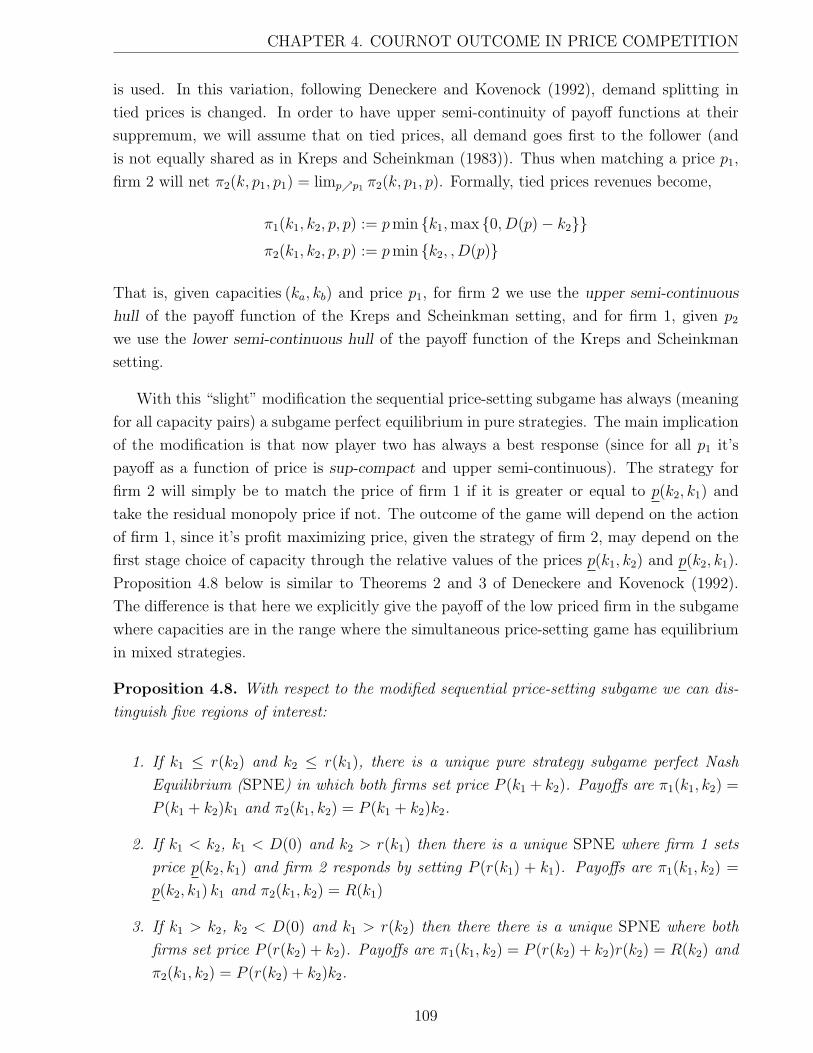
CHAPTER 4. COURNOT OUTCOME IN PRICE COMPETITION
is used. In this variation, following Deneckere and Kovenock (1992), demand splitting in
tied prices is changed. In order to have upper semi-continuity of payoff functions at their
suppremum, we will assume that on tied prices, all demand goes first to the follower (and
is not equally shared as in Kreps and Scheinkman (1983)). Thus when matching a price p1,
firm 2 will net π2(k, p1, p1) = limp↗p1 π2(k, p1, p). Formally, tied prices revenues become,
π1(k1, k2, p, p) := pmin {k1,max {0, D(p)− k2}}π2(k1, k2, p, p) := pmin {k2, , D(p)}
That is, given capacities (ka, kb) and price p1, for firm 2 we use the upper semi-continuous
hull of the payoff function of the Kreps and Scheinkman setting, and for firm 1, given p2
we use the lower semi-continuous hull of the payoff function of the Kreps and Scheinkman
setting.
With this “slight” modification the sequential price-setting subgame has always (meaning
for all capacity pairs) a subgame perfect equilibrium in pure strategies. The main implication
of the modification is that now player two has always a best response (since for all p1 it’s
payoff as a function of price is sup-compact and upper semi-continuous). The strategy for
firm 2 will simply be to match the price of firm 1 if it is greater or equal to p(k2, k1) and
take the residual monopoly price if not. The outcome of the game will depend on the action
of firm 1, since it’s profit maximizing price, given the strategy of firm 2, may depend on the
first stage choice of capacity through the relative values of the prices p(k1, k2) and p(k2, k1).
Proposition 4.8 below is similar to Theorems 2 and 3 of Deneckere and Kovenock (1992).
The difference is that here we explicitly give the payoff of the low priced firm in the subgame
where capacities are in the range where the simultaneous price-setting game has equilibrium
in mixed strategies.
Proposition 4.8. With respect to the modified sequential price-setting subgame we can dis-
tinguish five regions of interest:
1. If k1 ≤ r(k2) and k2 ≤ r(k1), there is a unique pure strategy subgame perfect Nash
Equilibrium (SPNE) in which both firms set price P (k1 + k2). Payoffs are π1(k1, k2) =
P (k1 + k2)k1 and π2(k1, k2) = P (k1 + k2)k2.
2. If k1 < k2, k1 < D(0) and k2 > r(k1) then there is a unique SPNE where firm 1 sets
price p(k2, k1) and firm 2 responds by setting P (r(k1) + k1). Payoffs are π1(k1, k2) =
p(k2, k1) k1 and π2(k1, k2) = R(k1)
3. If k1 > k2, k2 < D(0) and k1 > r(k2) then there there is a unique SPNE where both
firms set price P (r(k2) + k2). Payoffs are π1(k1, k2) = P (r(k2) + k2)r(k2) = R(k2) and
π2(k1, k2) = P (r(k2) + k2)k2.
109
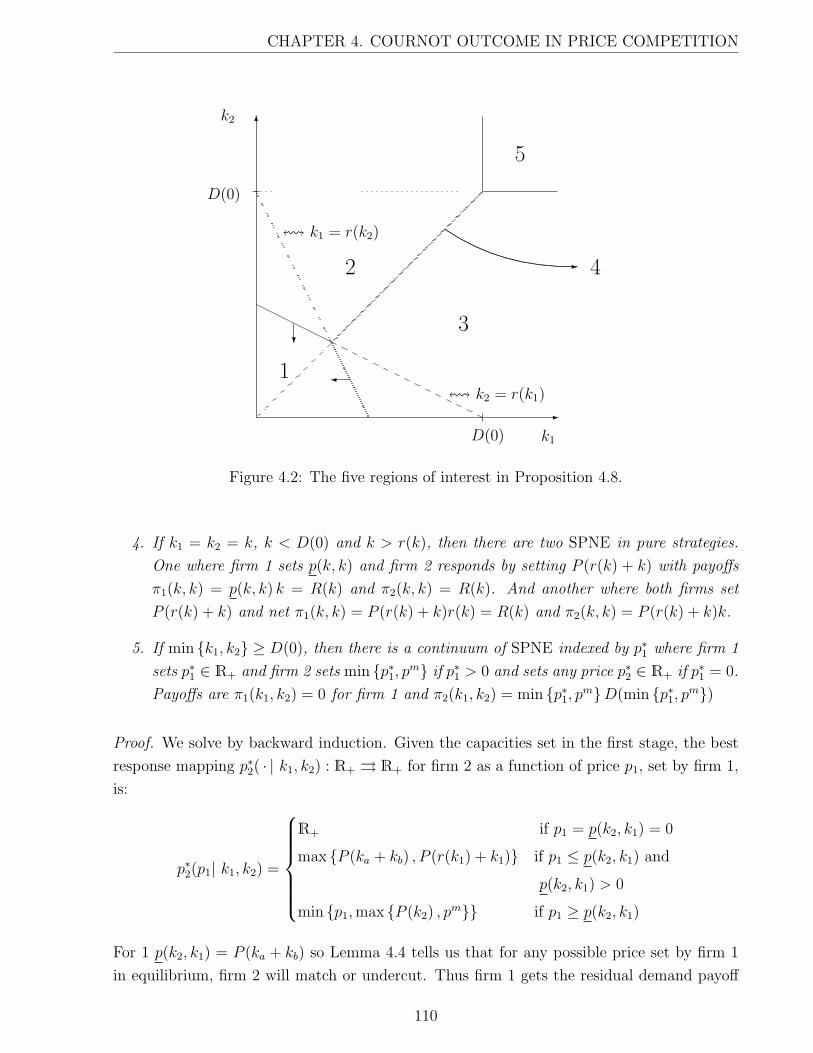
CHAPTER 4. COURNOT OUTCOME IN PRICE COMPETITION
6
-
D(0)
D(0)
3
! k2 = r(k1)
2
! k1 = r(k2)
1
5
�
?
k1
k2
...................
......................
........................................
........................................
.......................................
. ........................................ ......................................... .......................................... ........................................... - 4
Figure 4.2: The five regions of interest in Proposition 4.8.
4. If k1 = k2 = k, k < D(0) and k > r(k), then there are two SPNE in pure strategies.
One where firm 1 sets p(k, k) and firm 2 responds by setting P (r(k) + k) with payoffs
π1(k, k) = p(k, k) k = R(k) and π2(k, k) = R(k). And another where both firms set
P (r(k) + k) and net π1(k, k) = P (r(k) + k)r(k) = R(k) and π2(k, k) = P (r(k) + k)k.
5. If min {k1, k2} ≥ D(0), then there is a continuum of SPNE indexed by p∗1 where firm 1
sets p∗1 ∈ R+ and firm 2 sets min {p∗1, pm} if p∗1 > 0 and sets any price p∗2 ∈ R+ if p∗1 = 0.
Payoffs are π1(k1, k2) = 0 for firm 1 and π2(k1, k2) = min {p∗1, pm}D(min {p∗1, pm})
Proof. We solve by backward induction. Given the capacities set in the first stage, the best
response mapping p∗2( · | k1, k2) : R+ ⇒ R+ for firm 2 as a function of price p1, set by firm 1,
is:
p∗2(p1| k1, k2) =
R+ if p1 = p(k2, k1) = 0
max {P (ka + kb) , P (r(k1) + k1)} if p1 ≤ p(k2, k1) and
p(k2, k1) > 0
min {p1,max {P (k2) , pm}} if p1 ≥ p(k2, k1)
For 1 p(k2, k1) = P (ka + kb) so Lemma 4.4 tells us that for any possible price set by firm 1
in equilibrium, firm 2 will match or undercut. Thus firm 1 gets the residual demand payoff
110

CHAPTER 4. COURNOT OUTCOME IN PRICE COMPETITION
which is maximized at p∗1 = P (ka + kb).
For 2 given the strategy of firm 2, firm 1 nets the low priced firm payoff when setting
p1 < p(k2, k1) and the residual demand payoff when setting p1 > p(k2, k1). Since p(k1, k2) <
p(k2, k1), the only possibility for firm 1 to have a maximizer is to have upper semi-continuity
at p1 = p(k2, k1). And this only obtains if firm 2 sets P (r(k1) + k1).
In 3 we have p(k1, k2) > p(k2, k1) and thus firm 1 maximizes it’s payoff by setting
P (r(k2) + k2) at which firm 2 responds by matching.
In 5, p(k2, k1) = 0, so if p1 > 0 firm two will match or undercut and firm 1 will net 0.
Then, firm 1 can set, in equilibrium, any price p∗1 > 0, and firm 2 will match or undercut
depending on the value of p∗1. For the special case of p1 = 0, note that then firm 1 still nets
0 (so it is a possible strategy in equilibrium) and firm 2 nets 0 as well, so then firm 2 can
actually set any price in the price set. Thus any pair (0, p∗2), p∗2 ∈ R+ can be sustained as a
SPNE of the price game.
�
Suppose we have ka > kb and ka > r(kb), so that we stand in the case were in the simul-
taneous price game the equilibrium is in non degenerate mixed strategies and the residual
monopoly profit for firm a is greater than the market clearing profit. If firm b is the leader,
then it knows that if it sets a price higher than p(ka, kb) it will be undercut and then it
would get the residual demand, but since p(kb, ka) < p(ka, kb) firm b would net strictly more
by setting a price p(kb, ka) < pb ≤ p(ka, kb) since then firm a would rather take the residual
demand. On the other hand, if firm b is the follower, since it is the small firm, in order to
sell it’s whole production by being the low priced firm, it can set a bigger price than firm a
(P (kb) > P (ka)). Firm a then assumes it will be undercut and thus maximizes it’s payoff, as
the high priced firm, setting the residual demand monopoly price P (r(kb) + kb). Then, firm
b will set the same price (this is also true in the case ka = kb = k > r(k) since the rule assigns
first the demand to the follower and thus it will sell all it’s capacity). Then firm a will obtain a
payoff R(kb) with certainty and so it is indifferent between being leader or follower in the price
setting game, while firm b would rather go second since it nets p(ka, kb) kb if it is leader and
P (r(kb) + kb) kb if it is follower and in this capacity region we have P (r(kb) + kb) > p(ka, kb).
In Deneckere and Kovenock (1992) they address the “choice of roles” issue rising from this
observation, since we could say that if leadership were endogenized, then the large firm would
become leader. The small firm would wait for the announcement of the large firm, which
would then set the corresponding price first. The authors focus then on games of timing of
price announcement.
For the special case ka = kb = k > r(k) we have two SPNE, one where firms set different
111

CHAPTER 4. COURNOT OUTCOME IN PRICE COMPETITION
prices and one where both firms set the residual demand monopoly price, but only the second
one allows us to have upper semi-continuity of reduced payoff in the capacity setting game.
Since the first firm is indifferent between the two equilibria, we turn to upper semi-continuity
of payoffs to find possible non Cournot symmetric Nash equilibria of the reduced capacity
setting game in the next section. Regarding the second of these equilibria, because of the
rationing rule, the firm that announces it’s price in second place will net a strictly greater
payoff than the leader, therefore considering this SPNE we could say that both firms would
prefer to wait for the announcement of the rival before announcing it’s own price. The
rationing rule assigns the demand first to the follower, which is the sole difference between
roles for this strategy profile.
Proposition 4.8 ratifies what we had obtained in Proposition 4.6. Payoffs associated to
the SPNE of the modified sequential price subgame are exactly the same as those associated
to the equilibria of the original (sequential) one, explored in Proposition 4.6. Even more, in
the region where there was no pure strategy Nash equilibrium in the price subgame (case 4
in Proposition 4.6) we now have existence and uniqueness (except for the line k1 = k2) of
SPNE and the payoffs associated to this unique SPNE are precisely the ones mentioned in
Remark 4.7. This outlines the power of the Deneckere and Kovenock (1992) modification
of the sequential price game: changing the splitting rule on tied prices not only helps to
solve the mathematical problem of upper semi-continuity of payoffs, but also does not depart
from the intuitive outcome (nor in payoffs nor in strategies) of the price game in the original
setting, allowing to formally obtain these intuitive results over price competition with capacity
constraints when the small firm is follower. We see that the continuity problem being solved
by the Deneckere and Kovenock assumption on demand splitting on tied prices, does not
affect the economic conclusions of the model and effectively helps to clarify the behavior of
the agents.
4.2 Capacity Setting Reduced Game
Now that we have obtained all the SPNE of the prices-setting subgame, we can study
the capacity setting stage of the game. The usual approach would be to use reduced payoff
functions obtained from the outcomes of the subgame for each possible capacity pairs of the
first stage generating a capacity setting reduced game. The problem is that for the case of
ka = kb = k > r(k) we don’t have a unique payoff for the follower. So situations regarding one
of the firms setting a capacity ki greater than k∗ have to be studied carefully. Nevertheless,
let’s introduce the first stage capacity-setting game and the price-setting SPNE associated
payoffs.
In this stage firms set capacities simultaneously. They maximize their expected payoff of
112

CHAPTER 4. COURNOT OUTCOME IN PRICE COMPETITION
setting capacity ki knowing that the choice of the opponent will have an effect on the final
profit. When setting capacity, firms do not know whether they will set their price first or
second in the price-setting stage. This uncertainty may come, for instance, from the nature
of the variable under scrutiny. Capacity building or stock production may occur long before
price competition. Even more, once we enter the stage of price competition, and thinking in
some kind of endogenous timing or role in the price game, we have that the only preference
on roles is for the large firm being follower 5. As we have said, the small firm is indifferent
between announcing its price first or second. Thus it is not clear how long firms can wait
before being forced to announce a price. We will assume then that there is an exogenous
factor that determines the role in the price setting stage. Firms know, however, in the first
stage of the game, that there is a probability λi of being leader in the price game for firm
i, i ∈ {a, b}. In an incomplete information type of game, these distributions could represent
the probability of being impatient in the second stage of the game. They can be interpreted
as well as priors or beliefs of the firms about their role in the second stage price game.
Similarly, they induce priors onto the possible payoff outcomes (not necessarily roles) of this
subgame. Although we allow for the probabilities to be different for each firm and they could
well depend on the installed capacities, it is better, to keep track of the exercise, to think
of them as being equal to 1/2. As we will see below, the values of the probabilities λi are
irrelevant for the purpose of telling a neat economic story behind the Cournot outcome as a
result of price competition. These values become important when seeking for other equilibria
of the game, an issue that we address as well in what follows. The interpretation of these
distribution as priors may raise as well questions about their genesis. Questions for instance,
of endogenous generation of priors, which would inspire an exercise closely related to the
choice of roles (Hamilton and Slutsky 1990; Deneckere and Kovenock 1992; van Damme and
Hurkens 2004).
The capacity setting reduced game has as players the two firms, with strategy space R+
and payoff given by the function πi : R+ ×R+ → R,
πi(ki, kj) := λiπ1(ki, kj) +(1− λi) π2(kj, ki)− C(ki) (i, j) ∈ {(a, b) ,(b, a)}
where π1 and π2 are the profit functions obtained from the equilibria of the sequential price-
setting subgame described in Proposition 4.8.
5In the absence of naturally generated roles in sequential play (Gal-Or 1985; Amir and Stepanova 2006),Hamilton and Slutsky (1990) and van Damme and Hurkens (2004) study game forms where players chosewhen to play in a sequential game. When choosing the same timing it is assumed that the simultaneoussubgame equilibrium payoffs are obtained, which we prefer to avoid in this note, as Deneckere and Kovenock(1992) do in their work.
113
CHAPTER 4. COURNOT OUTCOME IN PRICE COMPETITION
Cournot Outcome
Regarding capacity setting competition, we first notice that the Cournot outcome is a
Subgame Perfect Nash equilibrium of the two-stage game with sequential price-setting, as
it was in the two-stage game with simultaneous price-setting stage case. If a firm sets the
Cournot capacity, then the opponent gets the Cournot payoff up to a certain capacity, namely
the Cournot best response for zero cost, and for greater capacities, since the higher capacity
firm nets the residual demand monopoly payoff no matter being leader or follower in the
second stage game, income remains fixed while cost increases.
Proposition 4.9. The Cournot outcome defined by ka = kb = k∗C and pa = pb = p∗C can be
sustained as a SPNE of the two-stage game.
Proof. Set k∗b = k∗C . Then k∗b < k∗ and thus Proposition 4.8 gives a unique reduced payoff
for firm a:
πa(ka, k∗C) =
P (ka + k∗C) ka − C(ka) if ka ≤ r(k∗C)
R(k∗C)− C(ka) if ka > r(k∗C)
As in Proposition 4.3, πa( · , k∗C) is continuous and if ka > r(k∗C) it is strictly decreasing.
Moreover, the function ka → kaP (ka + k∗C)−C(ka), the Cournot payoff function, attains it’s
maximum at k∗a = rC(k∗C) < r(k∗C) and thus ka = k∗b is the best response to k∗b = k∗C in the
reduced form capacity-setting game. Since the (unique) best response to k∗C in the reduced
form game is to set the same capacity and the game is symmetric, we conclude.
�
So now we have a clear neat story behind the Cournot outcome as the result of price
competition. If firms set small capacities, then price competition produces clear-market
prices. Facing Cournot capacity of the rival, a firm that sets a high capacity will net an
income that depends only on the capacity set by it’s rival. The large firm if being leader in
the price game knows it will be undercut. If being follower, the small firm will set the highest
price possible at which it can sell it’s whole capacity, that is, p(ki, kj) with ki > kj, the price
that leaves the high firm indifferent between matching and taking the residual demand, so
the large firm nets R(kj).
The Cournot outcome can be sustained as a subgame perfect equilibrium in pure strategies
at all stages of the game.
114

CHAPTER 4. COURNOT OUTCOME IN PRICE COMPETITION
Other Equilibria
Considering the possibility of other equilibria, note that setting the same capacity and
it being smaller than the value of the zero cost Cournot equilibrium k∗, can not be an
equilibrium since deviating to the Cournot best response maximizes payoff given the capacity
of the rival. It is the same argument as in the previous Proposition. This rules out any pure-
strategy Nash equilibrium with both capacities smaller than k∗.
However it could be possible to find symmetric Nash equilibria where firms engage in
higher capacities. Suppose that the expected reduced payoff (expectation taken over the
possibility of being leader or follower) in the first stage game, given that the rival plays a
capacity k strictly greater than the zero cost Cournot equilibrium k∗, is increasing in the
interval where there is a difference between being leader or follower, and that the expected
reduced payoff of matching this capacity is greater (or equal) than the maximum payoff that
could be attained by setting a capacity in the indifference (between being leader or follower)
interval (if not void); and consider the following strategies:
In the first stage set k. In the second stage, once roles are assigned, follow the
subgame perfect strategies given in Proposition 4.8. For the special case where
ka = kb = k let the leader set the price P (r(k) + k).
Then, using price leadership as a coordination device, the outcome(k, k)
can be sustained
as a SPNE of the game.
Indeed, once capacities are set, what follows has already been discussed. So the question
is: why would a firm set this capacity given that the other one did? The answer comes from
the possibility that the firm was follower in the second stage game because the follower can
set a relatively high price:
P(2k)< P
(r(k)
+ k).
First, notice that setting a higher capacity can not be a best response since payoff is decreasing
in that zone. Given the strategies in the price-setting subgame, upper semi-continuity of
reduced payoff gives the existence of the best response in the interval[0, k].
Second, note that reduced payoff for the small firm is of the form k → E[p |(k, k)]k−C(k)
where E[p |(k, k)]
is the expected price faced by a small firm. Expected price E[p |(k, k)]
for firm a against capacity k is given by:
E[p |(ka, k
)]=
P(ka + k
)if ka ≤ r−1
(k)
λap(k, ka
)+(1− λa)P (r(ka) + ka) if r−1
(k)≤ ka < k
115

CHAPTER 4. COURNOT OUTCOME IN PRICE COMPETITION
so that payoff for the small firm is continuous in[0, k[
and strictly greater than the Cournot
payoff for capacities in the interval]r−1(k), k[.
For the small firm as a second mover, when comparing6 the maximum profit from setting
a capacity k such that k < r−1(k)
and setting k, the fall in price (P(k + k
)↘ P
(r(k)
+ k)>
P(k + k
)) and the increase of the cost
(C(k)↗ C
(k))
may be compensated by the increase
in the volume of sales(k ↗ k
). The second mover price function, P (r(k) + k), is less steep
than the standard Cournot price function, allowing the possibility that payoff was increasing
in the interval]r−1(k), k[.
Second mover advantage has to be such that it drags sufficiently upwards the expected
payoff k → E[p |(k, k)]k − C(k) and the functions k → E
[p |(k, k)]
and k → −C(k) need
not be too strongly decreasing.
These two conditions can be written as find k such that:
P(r(k)
+ k) [λir(k)
+ (1− λi)k]− C
(k)≥ max
k∈[0,r−1(k)]P(k + k
)k − C(k) (4.2)
limk↗k
∂
∂k
[E[p |(k, k)]k − C(k)
]≥ 0 (4.3)
Condition (4.2) states that the payoff of matching is greater than the payoff of setting a ca-
pacity in the zone where there is no difference between being leader or follower, and condition
(4.3) states that the left hand derivative7 of the payoff function at the point k is positive
which, along with concavity of payoff in the region where there is difference between being
leader and follower and continuity at the point k = r−1(k), assures that payoff is maximized
at k = k.
We illustrate this situation with the following example:
Example 4.10. Consider the duopoly with price function P (q) = 1− q, and cost C(q) = cq
for both firms. The Cournot best response function is then:
rC(k) = max
{1− c− k
2, 0
}.
The zero-cost Cournot equilibrium is given by k∗ ≡ 1/3 and k∗C =(1− c) /3.
If λa = λb = 1/2 and c is sufficiently small then we can find a continuum of equilibria
along the line ka = kb. For instance for c ≡ 0.05, ka = kb = k = 0.3375 can be sustained by
a SPNE of the game and there is a continuum of Nash Equilibria along the line ka = kb in a
neighborhood of k. Of course, k∗C is not in this neighborhood.
6This comparison is relevant only if k ≤ r(0).7From the definition of p(ki, kj) when kj ↗ ki.
116
CHAPTER 4. COURNOT OUTCOME IN PRICE COMPETITION
Cournot Outcome and Contingent Demands
In Davidson and Deneckere (1986) Theorem 1 argues that the Cournot outcome can
not emerge as an equilibrium of the two stage game discussed by Kreps and Scheinkman
considering almost any rationing rule, in a certain class, different from the surplus maximizing
rationing rule. This is relevant as well for this work since the central argument states that
if we change the rationing rule then, given that in the first stage the set capacities were the
Cournot quantities, the Cournot price is not a best response to itself, ruling out as well the
Cournot outcome as the equilibrium of the sequential subgame. However the proof is made
only for the case of zero cost of capacity. As we will see below their result, as stated in their
work, is in fact only valid for this case and once there are costs a finer treatment becomes
necessary. Madden (1998) addresses this matter for a special setting that is not completely
compatible with the Kreps and Scheinkman or Davidson and Deneckere assumptions on the
demand function, but that enlightens what really is relevant when trying to answer the
question about how dependent are the results on the chosen rationing rule. Consider the
class of contingent demands that satisfy:
1. Di(pi|pj) downward-sloping twice differentiable except in pi = pj.
2. Di(pi|pj) = D(pi) for pi < pj
3. Di(pi|pj) = max{D(pi)
2, D(pi)− kj
}when pi = pj
4. max {0, D(pi)− kj} ≤ Di(pi|pj) ≤ max {0,min {D(pj)− kj, D(pi)}} for pi > pj
Both rationing rules: proportional and surplus maximizing satisfy points 1 to 4.
Suppose that contingent demand for the high priced firm is given by a C1 function
CD( · |pj, ki, kj) : R+ → R+ such that:
Di(pi|pj) =
D(pi) if pi < pj
max{D(pi)
2, D(pi)− kj
}if pi = pj
max {0, CD(pi|pj, kj, kj)} if pi > pj
and Di satisfies conditions 1 to 4. Note that for Di to satisfy conditions 1 to 4, we must
have that CD(pj|pj, kj, kj) = D(pj)− kj. Using the notation eCDq,p for the elasticity of demand
CD( · |p∗C , k∗C , k∗C) we can state the following proposition.
Proposition 4.11. If:
eCDq,p (p∗C) > −1 (4.4)
117

CHAPTER 4. COURNOT OUTCOME IN PRICE COMPETITION
then the Cournot outcome does not rise as the equilibrium of the two stage game (sequential
or simultaneous).
Proof. Suppose the two players set k∗C in the first stage. If player j sets price p∗C the payoff
for player i as a function of price is:
πi(p, p∗C , k
∗C , k
∗C) =
pk∗C p ≤ p∗C
pmax {0, CD(p|p∗C , k∗C , k∗C)} p > p∗C
This function is then continuous8 and increasing to the left of p∗C . The derivative to the right
of p∗C is
∂
∂pπi(p, p
∗C , k
∗C , k
∗C) = p CD′(p|p∗C , k∗C , k∗C) + CD(p|p∗C , k∗C , k∗C)
thus we have:
limp↓p∗C
∂
∂pπi(p, p
∗C , k
∗C , k
∗C) = p∗CCD
′(p∗C |p∗C , k∗C , k∗C) + CD(p∗C |p∗C , k∗C , k∗C)
= p∗CCD′(p∗C |p∗C , k∗C , k∗C) + k∗C
= k∗C
(p∗Ck∗CCD′(p∗C |p∗C , k∗C , k∗C) + 1
)> 0
Then p∗C /∈ argmaxp {πi(p, p∗C , k∗C , k∗C)}.
�
The proof follows the same ideas behind Davidson and Deneckere’s proof (1986). The
condition implies that payoff as a function of price, is increasing at the Cournot price. In
their result, the condition of Di(pi|pj) being locally distinct to the right from the surplus
maximizing contingent demand at the point pi = pj = p∗C when ki = kj = k∗C , is not sufficient
when costs are not equal to zero and is a special case of our condition (4.4). Condition (4.4)
is also in the line of Madden (1998), if the residual demand is not sufficiently elastic at the
Cournot price, then the Cournot outcome can not emerge as an equilibrium of the two stage
game.
8Since CD(p|p∗C , k∗C , k∗C) satisfies 2, limp↓p∗C CD(p|p∗C , k∗C , k∗C) = k∗C .
118

CHAPTER 4. COURNOT OUTCOME IN PRICE COMPETITION
5 Concluding Remarks
We have studied a three stage duopoly game where firms first set simultaneously capac-
ities and then engage in sequential price competition. We have related the outcome of the
sequential price game (Deneckere and Kovenock 1992) to the simultaneous price game (Kreps
and Scheinkman 1983) and we have obtained that the Cournot outcome of the market can
be sustained as a SPNE in pure strategies
Mixed strategies are a solution to the problem of existence in simultaneous price games.
However, there is still not a consensus about what a mixed strategy outcome represents in a
price game. Usual justifications for mixed strategy equilibria such as a population distribution
from where individuals are randomly selected to play the game, as in evolutionary game
theory do note seem appealing. Moreover, the fact that the pure strategies that are in the
support of the mixed strategy distributions are not necessarily best responses to the pure
strategies that are in the support of the rival’s mixed strategy distribution, gives rise to
the regret property of mixed strategies equilibria: once a realization of the distribution is
played, players may not be satisfied with the outcome, which is somehow incoherent with
Nash behavior or perfectness of equilibria (see for instance Vives (1999) and Friedman (1988)
for a discussion on Mixed strategies Nash equilibria in oligopoly games).
We have proposed in this note an alternative approach to the problem of existence of
equilibrium in pure strategies that is more in the line of Harsanyi (1973). Firms are uncertain
of their role in the price stage of the game. They know that sequential price competition will
take place, but since this competition is so far in the future, price leadership is unknown.
As in an incomplete information game, players know a probability distribution over their
roles in the price game and maximize expected payoff in the first stage. Price leadership
serves then as a coordination device that allows to obtain equilibrium outcomes in pure
strategies. It is important to notice that this result does not depend on the value of the
probability distribution, but only in the characteristics of the involved functions. That is,
on the structure of the market: cost of production, elasticity of demand. We have seen
that suitably and slightly modifying the sharing rule on tied prices it is possible to formally
reproduce the intuitively expected behavior of firms in the original setting (equal share at
tied prices).
Finally we have made space for the possibility of finding other symmetric quantity out-
comes sustained as SPNE depending only on primitives and on the probabilities of being
leader in the price game. No changes with respect to the Kreps and Scheinkman (1983)
setting have been made on cost or demand functions. The discussion is opened then on how
to treat such probabilities (endogenously generated, parameters of the model, firm indepen-
dent, etc.). Many lines of exploration can be taken: general n firm oligopoly, non symmetric
119

CHAPTER 4. COURNOT OUTCOME IN PRICE COMPETITION
cost structures of firms (Deneckere and Kovenock 1996) and effects of changes on contingent
demand (Davidson and Deneckere 1986), to give some examples.
120
CHAPTER 5
Conclusions
The main contributions of this thesis to Economic Theory and Mathematical Economics
are, on one hand the introduction of the concept of Rationalizability to a general class of
games with a continuum of players, and on the other hand, bringing together in an original
setting different areas of Economic Theory that remained until now relatively unrelated (large
games, rational expectations in economics).
In the area of large games, the main contribution is the formal and general definition of the
different sorts of Rationalizability in games with a continuum of players: Point-Rationalizable
Strategy profiles in games with a continuum of players (Definition 2.5), Point-Rationalizable
Sates in the particular case where payoffs depend on strategy profiles only through the value
of the integral (Definition 2.7), the extension of Rationalizability to non-point forecasts in this
same class of games by introducing Rationalizable States (Definition 2.21) and the definition
of Rationalizable Strategy Profiles in games where the set of actions of the players are finite
(Definition 2.25). Moreover, the main results are the characterizations of the sets of (Point-)
Rationalizable States (Theorems 2.10 and 2.22).
In Chapter 3 we have assessed stability of equilibria in a class of economic models where
forecasts of agents lie on the set of aggregate states. Relying on the general framework
introduced in Chapter 2 and the definitions of Rationalizability therein presented, we have
defined Strong Rationality (or Eductive Stability) as the uniqueness of the Rationalizable
solutions of the economic setting. We have studied as well the relation between this stability
concept and Iterative Expectational Stability in the general setting. The characterization of
Rationalizability has allowed for us as well to explore the local viewpoint to expectational
stability in this general setting as it has been done in more specific contexts in the literature.
An equilibrium is defined to be Locally Strongly Rational (or Locally Eductively Stable) if
121

CHAPTER 5. CONCLUSIONS
it is the unique result of the eductive process described in Theorem 2.10 of Chapter 2.
The main results of Chapter 3 are Theorems 3.30 and 3.40 in which we have endowed the
economic setting with a lattice structure in order to study the consequences over eductive sta-
bility of the presence of Strategic Complementarities and Strategic Substitutabilities. These
results can be summarized as follows: under the presence of Strategic Complementarities,
uniqueness of equilibrium assures it’s eductive stability while this is not necessarily true for
the case of Strategic Substitutes, where the study of the second iterate of a best-reply type
mapping may give a clue about this matter. We have as well shown that the sets of Equilibria
and Rationalizable States have some attractive mathematical structure. Moreover, through
Corollaries 3.32 and 3.42 we have shown the equivalence of the two stability concepts under
scrutiny in these two contexts.
Relevant mathematical results in these two Chapters, that risk to have remained un-
noticed, are Lemmas 2.6, which assures the necessary measurability properties of the best
response mapping as an operator over the players names, and 2.19, that expands continuity
properties to the case of general forecasts, in Chapter 2; and Lemmas 3.39 and 3.29, where
we show that the best-reply-to-forecasts mapping has appealing monotonicity properties, in
Chapter 3 that rely on the original result of Lemma 3.48, where we show that it is possible to
extract largest and smallest measurable selections from the best-reply mappings as functions
of the players’ names, in this same Chapter.
Finally, we have contributed in Chapter 4, with an interesting exercise, to the field of
oligopolistic competition. In such exercise, we present a duopoly in which firms engage in
capacity in a first stage and compete sequentially on prices on a second stage of a three stage
game. Price leadership is randomized, endowing the game with symmetry and allowing the
possibility of finding pure strategy subgame perfect equilibria, as it had not been done yet.
We have obtained as a result that the Cournot outcome of the duopoly can be sustained as
a Subgame Perfect Nash Equilibrium of the whole game, allowing to clearly interpret the
economic findings trough the sequence of play. We have as well obtained a sub product:
the possibility of finding non-Cournot outcomes, as a consequence of randomizing and the
attractiveness of being second mover in the price-setting subgame. We have provided a
sufficient condition for the existence of such equilibrium outcomes.
We expect that Chapters 2 and 3 altogether may open the scope of related research by
providing a general framework, original tools and pertinent links and relations between the
different elements that have been studied therein; that we hope will prove to be useful in
what will follow.
122

Bibliography
Aliprantis, Charalambos D., and Kim C. Border. 1999. Infinite Dimensional Analysis A
Hitchhiker’s Guide. 3rd. Berlin: Springer-Verlag.
Allen, Beth, and Martin Hellwig. 1986. “Price-Setting Firms and the Oligopolistic Founda-
tions of Perfect Competition.” The American Economic Review 76 (2): 387–392 (May).
Papers and Proceedings of the Ninety-Eighth Annual Meeting of the American Economic
Association.
Amir, Rabah, and Anna Stepanova. 2006. “Second-mover advantage and price leadership
in Bertrand duopoly.” Games and Economic Behavior 55 (1): 1–20 (April).
Apt, Krzysztof R. 2007. “The Many Faces of Rationalizability.” The B.E. Journal of
Theoretical Economics 7 (1): Article 18.
Aumann, Robert J. 1965. “Integrals of Set-Valued Functions.” Journal of Mathematical
Analysis and Applications 12:1–12.
. 1976. “An elementary proof that integration preserves uppersemicontinuity.” Jour-
nal of Mathematical Economics 3:15–18.
Basu, Kaushik, and Jorgen W. Weibull. 1991. “Strategy subsets closed under rational
behavior.” Economics Letters 36 (2): 141–146 (June).
Berge, C. 1997. Topological Spaces. Dover Publications.
Bernheim, B. Douglas. 1984. “Rationalizable Strategic Behavior.” Econometrica 52 (4):
1007–1028 (July).
Bertrand, J. 1883. “Theorie Mathematique de la Richesse Sociale.” Journal des Savants
67 (Septembre): 499–508.
123
Bibliography
Chamley, Christophe. 1999. “Coordinating Regime Switches.” The Quarterly Journal of
Economics 114 (3): 869–905 (August).
Chamley, Christophe P. 2004. Rational Herds: Economic Models of Social Learning. Cam-
bridge University Press.
Chatterji, Shurojit, and Sayantan Ghosal. 2004. “Local coordination and market equilibria.”
Journal of Economic Theory 114 (2): 255–279 (February).
Chen, Yi-Chun, Ngo Van Long, and Xiao Luo. 2007. “Iterated strict dominance in general
games.” Games and Economic Behavior 61 (2): 299–315 (November).
Cooper, Russell W. 1999. Coordination Games: Complementarities and Macroeconomics.
Cambridge, UK: Cambridge University Press.
Dastidar, Krishnendu Ghosh. 2004. “On Stackelberg games in a homogeneous product
market.” European Economic Review 48 (3): 549–562 (June).
Davidson, Carl, and Raymond Deneckere. 1986. “Long-Run Competition in Capacity, Short-
Run Competition in Price, and the Cournot Model.” The Rand Journal of Economics
17 (3): 404–415 (Autumn).
DeCanio, Stephen J. 1979. “Rational Expectations and Learning from Experience.” The
Quarterly Journal of Economics 93 (1): 47–57 (Feb.).
Deneckere, Raymond J., and Dan Kovenock. 1992. “Price Leadership.” The Review of
Economic Studies 59 (1): 143–162 (January).
. 1996. “Bertrand-Edgeworth duopoly with unit cost asymmetry.” Economic Theory
8 (1): 1–25 (June).
Desgranges, Gabriel. 2000, August. “CK-Equilibria and Informational Efficiency in a Com-
petitive Economy.” Econometric society world congress 2000 contributed papers 1296,
Econometric Society.
Desgranges, Gabriel, and Stephane Gauthier. 2004. “Competition and Cordination of
Expectations.” mimeo.
Desgranges, Gabriel, and Maik Heinemann. 2005, March. “Strongly rational expec-
tations equilibria with endogenous acquisition of information.” Working paper se-
ries in economics 9, University of Luneburg, Institute of Economics. available at
http://ideas.repec.org/p/lue/wpaper/9.html.
Dixon, Huw David. 1992. “The Competitve Outcome as the Equilibrium in an Edgeworthian
Price-Quantity Model.” The Economic Journal 102 (March): 301–309.
Dufwenberg, Martin, and Mark Stegeman. 2002. “Existence and Uniqueness of Maxi-
mal Reductions under Iterated Strict Dominance.” Econometrica 70 (5): 2007–2023
(September).
124

Bibliography
Edgeworth, Francis. 1925. “The Pure Theory of Monopoly.” In Papers Relating to Political
Economy, Volume 1, 111–142. Royal Economic Society.
Evans, George W., and Roger Guesnerie. 1993. “Rationalizability, Strong Rationality and
Expectational Stability.” Games and Economic Behavior 5:632–646.
. 2003. “Coordination on Saddle-Path Solutions: The Eductive Viewpoint–Linear
Univariate Models.” Macroeconomic Dynamics 7 (1): 42–62.
. 2005. “Coordination on saddle-path solutions: the eductive viewpoint–linear mul-
tivariate models.” Journal of Economic Theory 124 (2): 202–229 (October).
Friedman, James W. 1988. “On the Strategic Importance of Prices versus Quantities.” The
RAND Journal of Economics 19 (4): 607–622.
Gal-Or, Esther. 1985. “First Mover and Second Mover Advantages.” International Economic
Review 26 (3): 649–653 (October).
Guesnerie, Roger. 1992. “An Exploration on the Eductive Justifications of the Rational-
Expectations Hypothesis.” The American Economic Review 82 (5): 1254–1278 (Decem-
ber).
. 2001. Assesing Rational Expectations: Sunspot Multiplicity and Economic Fluctu-
ations. MIT Press.
. 2002. “Anchoring economic predictions in common knowledge.” Econometrica 70
(2): 439 (March).
. 2005. “Strategic Substitutabilities versus Strategic Complementarities: Towards a
General Theory of Expectational Coordination?” Revue d’Economie Politique 115 (4):
393–412 (July–August).
Guesnerie, Roger, and Pedro Jara-Moroni. 2007. “Expectational coordination in a class of
economic models: Strategic substitutabilities versus strategic complementarities.” Pse
working papers 2007-28, PSE (Ecole normale superieure).
Hamilton, Jonathan H., and Steven M. Slutsky. 1990. “Endogenous timing in duopoly
games: Stackelberg or cournot equilibria.” Games and Economic Behavior 2 (1): 29–46
(March).
Harsanyi, J. 1973. “Games With Randomly Disturbed Payoffs: A New Rationale for
Mixed-Strategy Equilibrium Points.” International Journal of Game Theory 2:1–25.
Jara-Moroni, Pedro. 2008a. “The Cournot Outcome as the Result of Price Competition.”
Pse working papers 2007-24, PSE (Ecole normale suprieure).
. 2008b. “Rationalizability in games with a continuum of players.” Pse working
papers 2007-25, PSE (Ecole normale suprieure).
125

Bibliography
Khan, M. Ali, and Nikolaos S. Papageorgiou. 1987. “On Cournot-Nash Equilibria in Gen-
eralized Qualitative Games with an Atomless Measure Space of Agents.” Proceedings of
the American Mathematical Society 100 (3): 505–510 (July).
Khan, M. Ali, Kali P. Rath, and Yeneng Sun. 1997. “On the Existence of Pure Strategy
Equilibria in Games with a Continuum of Players.” Journal of Economic Theory 76:13–
46.
Khan, M. Ali, and Yeneng Sun. 2002. “Non-Cooperative Games with Many Players.” In
Handbook of Game Theory, edited by R. Aumann and S. Hart, Volume 3, 1761–1808.
Elsevier Science.
Kreps, David M., and Jose A. Scheinkman. 1983. “Quantity Precommitment and Bertrand
Competition Yield Cournot Outcomes.” The Bell Journal of Economics 14 (2): 326–337
(Autumn).
Levitan, Richard, and Martin Shubik. 1972. “Price Duopoly and Capacity Constraints.”
International Economic Review 13 (1): 111–122 (February).
Lucas, Robert E., Jr. 1978. “Asset Prices in an Exchange Economy.” Econometrica 46 (6):
1429–1445 (November).
Madden, Paul. 1998. “Elastic demand, sunk costs and the Kreps-Scheinkman extension of
the Cournot model.” Economic Theory 12 (1): 199–212 (June).
Mas-Colell, Andreu. 1984. “On a theorem of Schmeidler.” Journal of Mathematical Eco-
nomics 13 (3): 201–206 (December).
Milgrom, Paul, and John Roberts. 1990. “Rationalizability, Learning, and Equilibrium in
Games with Strategic Complementarities.” Econometrica 58 (6): 1255–1277 (Novem-
ber).
Morris, Stephen, and Hyun Song Shin. 1998. “Unique Equilibrium in a Model of Self-
Fulfilling Currency Attacks.” American Economic Review 88 (3): 587–597 (June).
Muth, John F. 1961. “Rational Expectations and the Theory of Price Movements.” Econo-
metrica 29 (3): 315–335 (July).
Osborne, Martin J., and Carolyn Pitchik. 1986. “Price competition in a capacity-constrained
duopoly.” Journal of Economic Theory 38 (2): 238–260.
Pearce, David G. 1984. “Rationalizable Strategic Behavior and the Problem of Perfection.”
Econometrica 52 (4): 1029–1050 (July).
Rath, Kali P. 1992. “A direct proof of the existence of pure strategy equilibria in games
with a continuum of players.” Economic Theory 2:427–433.
Reny, Philip J. 1999. “On the Existence of Pure and Mixed Strategy Nash Equilibria in
Discontinuous Games.” Econometrica 67 (5): 1029–1056 (sep).
126

Bibliography
Rockafellar, R.T., and Roger J.-B. Wets. 1998. Variational Analysis. Springer.
Schmeidler, David. 1973. “Equilibrium points of nonatomic games.” Journal of Statistical
Physics 7 (4): 295–300 (April).
Tan, Tommy Chin-Chiu, and Sergio Ribeiro da Costa Werlang. 1988. “The Bayesian
Foundations of Solution Concepts of Games.” Journal of Economic Theory 45 (2):
370–391 (August).
Topkis, Donald M. 1998. Supermodularity and complementarity. Frontiers of economic
research. Princeton University Press.
Townsend, Robert M. 1978. “Market Anticipations, Rational Expectations, and Bayesian
Analysis.” International Economic Review 19 (2): 481–494 (jun).
van Damme, Eric, and Sjaak Hurkens. 2004. “Endogenous price leadership.” Games and
Economic Behavior 47:404–420.
Vives, Xavier. 1986. “Commitment, flexibility and market outcomes.” International Journal
of Industrial Organization 4 (2): 217–229 (June).
. 1990. “Nash Equilibrium With Strategic Complementarities.” Journal of Mathe-
matical Economics 19:351–321.
. 1999. Oligopoly Pricing: Old Ideas and New Tools. Cambridge, MA: MIT Press.
127