geotecnia

11

TEORÍA COULOMB - RANKINE (1857)

TEORIA DE RANKINE Y EQUILIBRIO PLASTICO

TEORÍA DE COULOMB (1776)

EFECTOS A CONSIDERAR

EJERCICIO

INDICE

Indice

22

• Seguridad ante el deslizamiento• Seguridad contra falla por vuelco • Factor de Seguridad respecto a la base (1/3 central)• Estructura segura contra asentamientos excesivo• Presión bajo la base no debe exceder la presión admisible

EMPUJE DE TIERRAS( Teoría Coulomb - Rankine 1857 )

Objetivo: Permite evaluar requisitos para el diseño de estructuras de contención

Teorías: Las mas empleadas son las de Coulomb y Rankine. Sus resultados son conservadores ( permiten el cálculo de estructuras decontención hasta 5 ó 6 m ).

Hipótesis de cálculo :• Suelo homogéneo• Posibilidad de desplazamiento del muro• Superficie de rotura del suelo es plana• Empuje es normal al muro ( pared lisa y

vertical)• Coronamiento horizontal

θθθθEa

δ = 0δ = 0δ = 0δ = 0

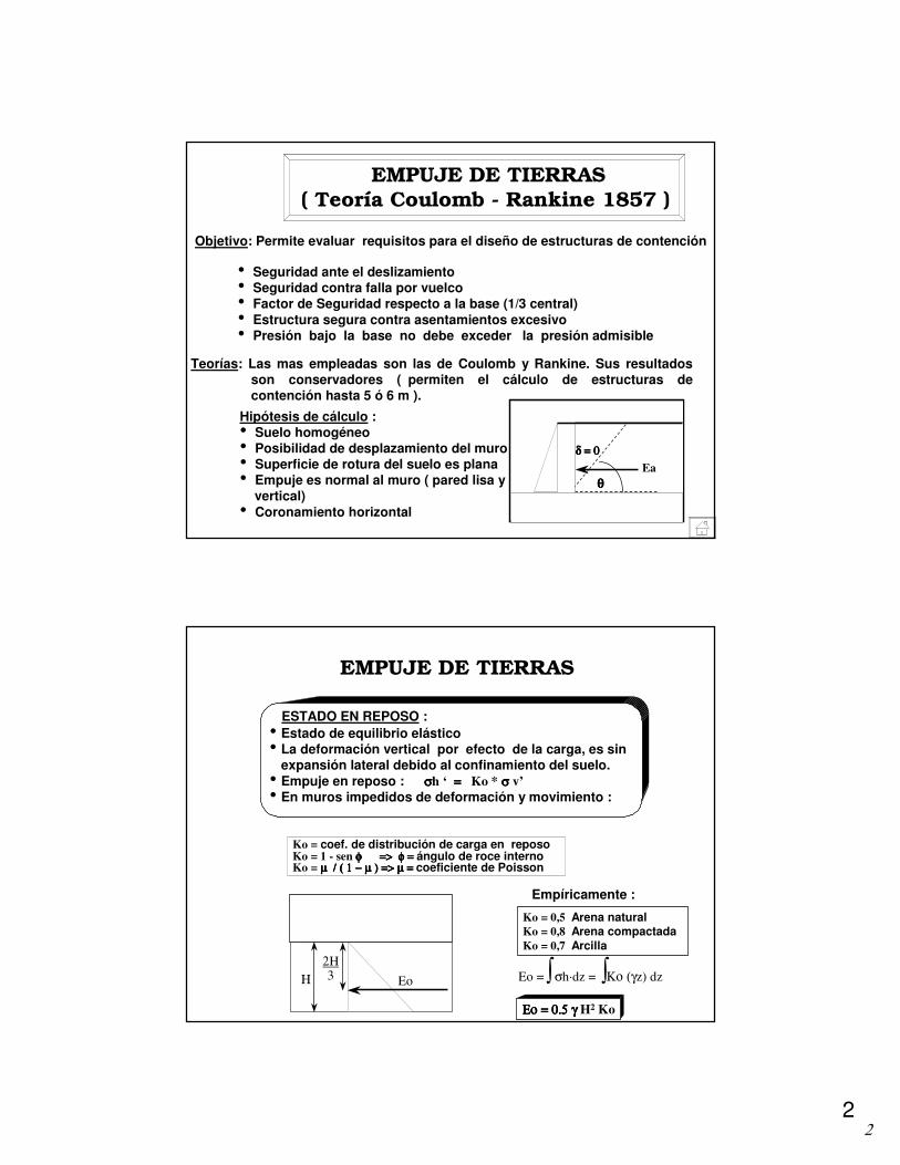
EMPUJE DE TIERRAS

ESTADO EN REPOSO :• Estado de equilibrio elástico• La deformación vertical por efecto de la carga, es sin

expansión lateral debido al confinamiento del suelo.• Empuje en reposo : σσσσh ‘ ==== Ko * σ σ σ σ v’• En muros impedidos de deformación y movimiento :

Eo =� σh·dz = �Κο (γz) dz

ΕοΕοΕοΕο = 0.5 γ = 0.5 γ = 0.5 γ = 0.5 γ H2 Ko

Η Eo2H3

Ko = coef. de distribución de carga en reposoKo = 1 - sen φ => φ = φ => φ = φ => φ = φ => φ = ángulo de roce internoKo = µ / ( 1 µ / ( 1 µ / ( 1 µ / ( 1 −−−− µ ) => µ = µ ) => µ = µ ) => µ = µ ) => µ = coeficiente de Poisson

Ko = 0,5 Arena naturalKo = 0,8 Arena compactadaKo = 0,7 Arcilla

Empíricamente :

33

ESTADO EN REPOSO :

• Estado de equilibrio elástico• La deformación vertical por efecto de la carga, es sin expansión

lateral debido al confinamiento del suelo.• Empuje en reposo : σσσσh ‘ ==== Ko * σ σ σ σ v’• En muros impedidos de deformación y movimiento :

Eo =� σh·dz = �Κο (γz) dz

ΕοΕοΕοΕο = 0.5 γ = 0.5 γ = 0.5 γ = 0.5 γ H2 Ko

Η Eo2H3

Ko = coef. de distribución de carga en reposoKo = 1 - sen φ => φ = φ => φ = φ => φ = φ => φ = ángulo de roce internoKo = µ / ( 1 µ / ( 1 µ / ( 1 µ / ( 1 −−−− µ ) => µ = µ ) => µ = µ ) => µ = µ ) => µ = coeficiente de Poisson

Ko = 0,5 Arena naturalKo = 0,8 Arena compactadaKo = 0,7 Arcilla

Empíricamente :

K a = σ σ σ σ Η Η Η Η = 1 1 1 1 = 1 = = 1 = = 1 = = 1 = 1 - sen φ φ φ φ σ σ σ σ V tg2( π / 4 + φ / 2 ) ( π / 4 + φ / 2 ) ( π / 4 + φ / 2 ) ( π / 4 + φ / 2 ) Ν φ Ν φ Ν φ Ν φ 1 + sen φ φ φ φ

ESTADO ACTIVO :

• El muro se mueve•Los elementos de suelo se expanden •El esfuerzo vertical permanece constante, pero esfuerzo lateral se reduce•Se alcanza la falla por corte o equilibrio plástico.•K no disminuye más => K = Ka

σ σ σ σ 1111 = σ = σ = σ = σ V = σ = σ = σ = σ 3333 Ν φ + 2 Ν φ + 2 Ν φ + 2 Ν φ + 2 c √√√√ N φ = φ = φ = φ = σσσσH Ν φ + 2 Ν φ + 2 Ν φ + 2 Ν φ + 2 c √√√√ N φ φ φ φ Si c = 0

Relleno: c , φ, γ

Eas

qs

Ea q Ea c

44

entonces, σσσσh = Ka σσσσ v −−−− 2 2 2 2 c √√√√ Ka y Ea = �� σσσσh dz

Ea = 1/2 γ γ γ γ H2 Ka - 2 c H Ka + qs H Ka

Finalmente el caso general con sobrecarga y cohesión es:

σσσσh = Ka ( γ γ γ γ z + qs ) −−−− 2 2 2 2 c √√√√ Ka 0

H

σσσσ1 = σσσσ3 Nφφφφ + 2c NφφφφSi σσσσ v >>>> σσσσh = > σσσσ v ==== σσσσh Nφφφφ + 2c NφφφφPor lo tanto , σσσσh = σσσσ v //// Nφφφφ −−−− 2 2 2 2 c / / / / Nφφφφ

pero ,,,, Ka = 1 / N φφφφ

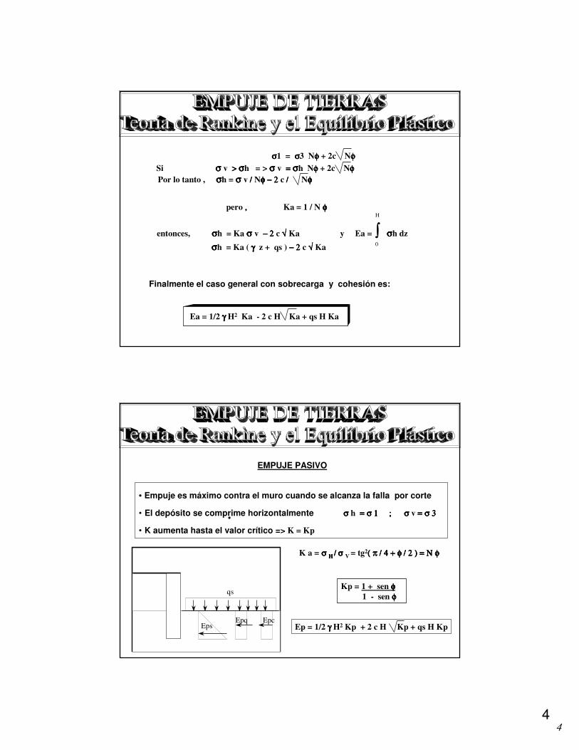
EMPUJE PASIVO

• Empuje es máximo contra el muro cuando se alcanza la falla por corte

• El depósito se comprime horizontalmente σ σ σ σ h = σ 1 ; σ = σ 1 ; σ = σ 1 ; σ = σ 1 ; σ v = σ 3 = σ 3 = σ 3 = σ 3

• K aumenta hasta el valor crítico => K = Kp •

Ep = 1/2 γ γ γ γ H2 Kp + 2 c H Kp + qs H Kp

Kp = 1 + sen φφφφ1 - sen φ φ φ φ

EpsEpq Epc

qs

K a = σ σ σ σ Η Η Η Η //// σ σ σ σ V = tg2( π / 4 + φ / 2 ) = Ν φ ( π / 4 + φ / 2 ) = Ν φ ( π / 4 + φ / 2 ) = Ν φ ( π / 4 + φ / 2 ) = Ν φ

55

Según lo analizado, se presentan tres estados en la masa de suelo :

ΚΚΚΚpσσσσvKaσσσσv σvσ

τ

Koσσσσv

σ σ σ σ h activo < σ σ σ σ h reposo < σσσσ h pasivoLos dos últimos son estados de tensión en situaciones extremas

4Estado de Reposo

4Estado Activo4Estado Pasivo

EMPUJE DE TIERRASTeoría de Coulomb (1776)

Esta teoría de empuje de tierras, incluye el efecto de fricción del suelo con el muro; es aplicable a cualquier inclinación de muro y a rellenos inclinados

Condiciones :•La superficie de deslizamiento es plana•Existen fuerzas que producen el equilibrio de la cuña

Cuña plana soportada por la reacción del muro R y la del suelo W.

cos ( β − φ ) / cos βKa =

cos ( β + δ ) + sen ( φ + δ ) sen ( φ - i )cos ( β − i )

2

i

δ = 2/3 − 3/4 φ

β

EaW

H

δ = 1/3 − 2/3 φ

θ

W = f ( γ )

R = f (φ)E = f (δ)

66

EMPUJE DE TIERRASEfectos a considerar

• Disminuye el empuje activo , por lo tanto, es favorable económicamente ( menor dimensión de la estructura )

• La cohesión se opone a la extensión, por lo que se generan esfuerzos de tracción que se traducen en grietas hasta Zc, llevando el empuje activo casi al valor nulo

• Efecto Hidrostático : Empuje del agua ( γ γ γ γ w )• Efecto del suelo : Empuje sólo de las partículas del

suelo, independiente del efecto del agua ( γ γ γ γ b )

COHESION

AGUA

Zc

Ea = γ (z -Zc)KaC

T

γω Η γ b Η Κa γ ω(Η−h) (γ Η+γb (H-h))Ka

EJERCICIO : EMPUJE DE TIERRAS

Un muro de 5m de altura cuyo paramento interior es vertical y liso, sostiene un terraplén sin cohesión , cuyo ángulo de roce interno es 32

��

, índice de vacíos de 0,53 , peso específico del sólido de 2,70 T/m3 y humedad de saturación de 19,6%.Calcular el empuje activo para los siguientes casos :

γd = γs /( 1 + e ) = 1,76 T/m3Ka = (1 - sen φ ) /( 1 + sen φ) = 0,31

Ea = 1/2 γd H2 KaEa = 1/2·1,76·25·0,31 = 6,82 T/ml

B. El terraplén está sumergido

γ sat = 2,1 T/m3Ea = 1/2 γ b H2 KaEa = 1/2·( 2,1 - 1,0 )·25·0,31 = 4,28 T/ml

A. El terraplén está seco

Es

ΕωEsΕω

77

C. Sólo el terraplén está sumergido

Ea = 1/2 γb H2 Ka + 1/2 γw H2

Ea = 1/2·1,1·25·0,31 + 1/2·1·25 = 16,78 T/ml

D. El nivel freático se encuentra a - 2,00 m en la zona del terraplén y sobre éste el suelo está saturado por capilaridad

Ea = 1/2·γsat·H2·Ka + 1/2·γb·H2·Ka + 1/2·γw·H2 + q·H·KaEa = 1/2·2,1·4·0,31 + 1/2·1,1·9·0,31+ 1/2·1·9 + (2,1·2 )·3·0,31Ea = 11,24 T/ml

ΕωEs

ΕωEs

Es

Eq

EJERCICIO : EMPUJE DE TIERRAS

PRINCIPALES FUERZAS SOBRE EL MURO

TIPOS DE ESTRUCTURAS DE CONTENCION

REQUISITOS

ETAPAS Y RECOMENDACIONES

EMPUJES SISMICOS

CONTROL DE CALIDAD

Indice

88

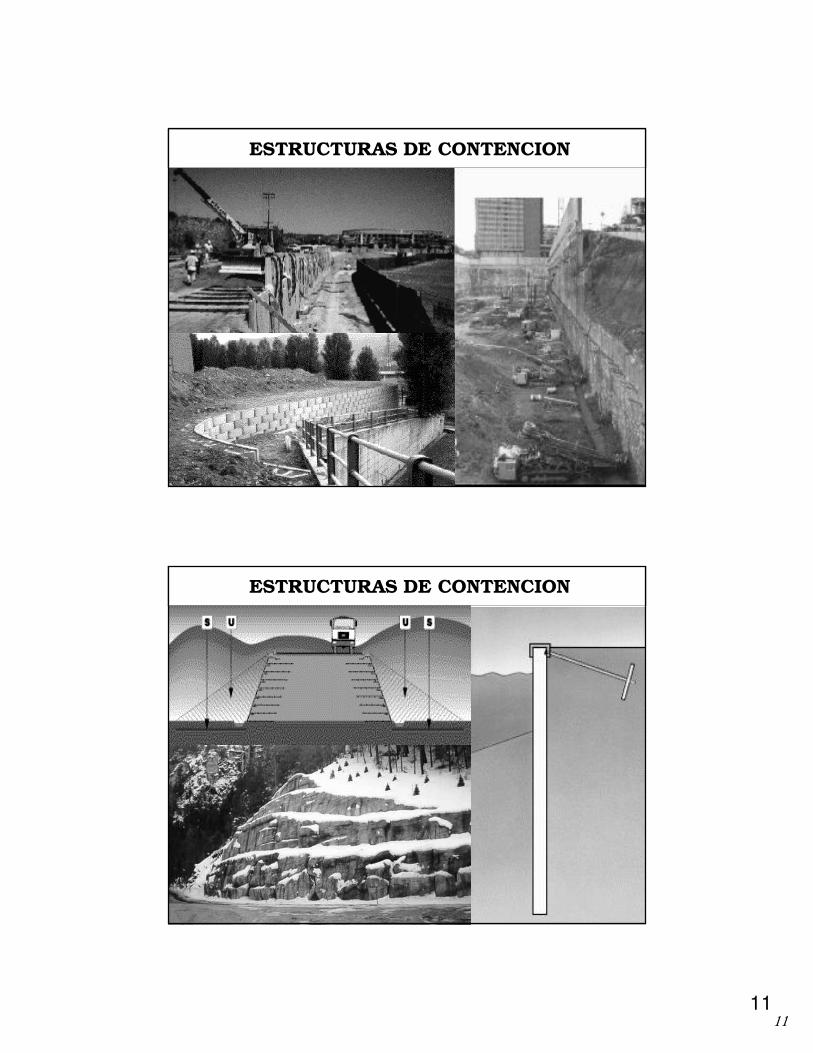
ESTRUCTURAS DE CONTENCION

�Empuje activo y pasivo�Peso propio del muro�Rozamiento suelo-muro en trasdos y base del muro (Si δ δ δ δ = 0 =>Mayor FS )�Fuerzas dinámicas�Napa freática�Sobrecargas�Fuerzas de expansión del suelo

El método de diseño de estructuras de contención consiste en estudiar lasituación en el momento de falla, a través de teorías de estado límite, y luego introducir un FS para evitar el colapso.PRINCIPALES FUERZAS QUE ACTUAN SOBRE LA ESTRUCTURA DE CONTENCION :

δ base - suelo

W

Ea sísmico

Ea sueloEpw

Eps

EpsEqs

δ trasdos

TIPOS DE ESTRUCTURAS DE CONTENCION

Tipos de estructuras de contención

Rígidas: muros Flexibles

HormigónMampostería Especiales TablestacadosPantallas

In situ

Continuas

En masa o de gravedad

Armado

• En L• En T• De contrafuerte• Aligerado

DiscontinuasPilotes independientes

Micropilotes

De pilotesIndependientes

SecantesTangentes

De panelesArmados

Pretensados

Entibaciones con varios niveles de

apoyo

De paneles prefabricados

Tierra armadamuros jaula o cribaSuelos reforzados

99

TIPOS DE ESTRUCTURAS DE CONTENCIONEstructuras Rígidas

Mampostería Hgón en masa En “ T “ En “ L “

Contrafuerte Muro jaula Tierra Armada

ArmaduraMetálica

Suelo Reforzado

Geosintéticos

Hormigón

TIPOS DE ESTRUCTURAS DE CONTENCIONEstructuras Flexibles

Tablaestaca anclada

Pantalla in situarmada y anclada

Pantalla in situpretensada

MicropilotesPaneles

prefabricadosPilotes

independientesPilotes

tangentes

Tablaestacadoen voladizo

Bentonitay cemento

1010

ESTRUCTURAS DE CONTENCION FLEXIBLES

Muro de mamposteria

Muro jaula

ESTRUCTURAS DE CONTENCION FLEXIBLESMuros Pantalla

1111



1212

• Factor de seguridad al deslizamientoFSD = Fuerzas resistentes = Ep + W tg δ δ δ δ > 1,0

Fuerzas deslizantes Ea

•Factor de seguridad al volcamiento FSV = Momentos resistentes = M ( Ep) + M ( W ) > 1,0

Momentos volcantes M ( Ea )

•Resultante de las fuerzas debe pasar por el tercio central de la base del muro

•La estructura de fundación deberá ser resistente para evitar roturas o asentamientos del subsuelo

•Resistencia a fuerzas de origen sísmico

ESTRUCTURAS DE CONTENCIONRequisitos

1. PREDIMENSIONAMIENTO :

•Albañilería de piedra u hormigón . B = 0,4 - 0,5 H

•Muros en T : Parte del suelo contribuye a la estabilidad del murod1 = H/10 - H/8d2 = H/12 - H/10d3 = 15 a 30 cmB = 0,40 - 0,66 H

2. Cálculo del EMPUJE ACTIVO conociendo las propiedades del suelo enel trasdós ( γ , φ , σγ , φ , σγ , φ , σγ , φ , σ adm , c )

3. Cálculo del PESO del muro

4. Cálculo de la FUERZA RESULTANTE y la posición de su línea de acción x, la cual debe encontrarse en el 1/3 central de la base del muro

H

d3

d1 d2B

1313

5. Cálculo de la CAPACIDAD DE SOPORTE del suelo, estática y dinámica, laque debe ser mayor o igual a las fatigas aplicadas por el muro al suelo.

6. Cálculo del FACTOR DE SEGURIDAD AL DESLIZAMIENTO.Valores recomendados : ( Dujisin y Rutllant, 1974 )

FS estático FS dinámicoRelleno cohesivo 1,8 1,4Relleno granular 1,4 1,2

7. Cálculo del FACTOR DE SEGURIDADCONTRA EL VOLCAMIENTO.Valores recomendados : ( Dujisin y Rutllant, 1974 )

FS estático FS dinámicoRelleno cohesivo 2,0 1,5Relleno granular 1,5 1,2

8. Cálculo del EMPUJE SÍSMICO , incluyendo fuerzas horizontales equivalentes, consistentes en un porcentaje del peso del muro

ESTRUCTURAS DE CONTENCIONEmpujes Sísmicos -Mononobe y Okabe

HIPÓTESIS:

• El muro se desplazará para producir presión activa• Al generarse la presión activa, se produce resistencia al corte máxima• La cuña se comporta como cuerpo rígido, por lo tanto, las fuerzas

actuantes se representan por :

Propuesta en Japón después del terremoto de 1923. Se desarrolla en una extensión pseudoestática de la solución de Coulomb, donde fuerzas estáticas horizontales y verticales actúan por sobre la cuña estática, generando el empuje total sísmico en el muro.

donde : W = peso de la cuñaKv, Kh = coeficientes sísmicos

horizontal y vertical

Fh = Kh · WFv = Kv · W

Τ

βδ

ΝW

Kv·W

Kh·W

i

1414

Ea = 1/2 γ γ γ γ H2 Ka=> ∆∆∆∆ Eas = 1/2 γ Ηγ Ηγ Ηγ Η2 2 2 2 ( Kas ( 1 - Kv) - Ka ))

La resultante de ∆∆∆∆ Eas actúa a 2/3 H medido desde la base

θ =θ =θ =θ = arctg ( Kh / ( 1 - Kv ) )Kh = 500 / S0.25 (e0,70250,70250,70250,7025 ΜΜΜΜ/ ( R + 60 ) 2,71 )

ESTRUCTURAS DE CONTENCIONEmpujes Sísmicos -Mononobe y Okabe

Eat = Ea + ∆ ∆ ∆ ∆ Eas

β

δ

i

H

∆EasEsa

( ) ( ) ( )( )

2

i�cosi�sen��sen��cos

cos ��)cos( �

Ka

��

�

�

��

�

�

−−−++

−

=

( )

( ) ( ) ( )( ) ( )

2

2

2

coscossensen

1coscoscos

cos

��

��

−++−−++++

−−=

βθβδθφδφθβδβθ

βθφ

ii

Kas

Eat = 1/2 γ γ γ γ H2 Kas ( 1 - Kv)

Según Saragoni et.al : a = 2300 e cm/seg2( R + 60 )

V = 4073,450 e cm / seg( R + 60 )

R = magnitud Richter del sismoM = distancia hipocentral del lugar en km.

1,6

0,71 M

0,34 M

3,02

ESTRUCTURAS DE CONTENCIONElección del coeficiente sísmico

Para elegir Kh y Kv, se deben suponer iguales a la máxima aceleración H y V , divididos por g ( aceleración de gravedad )Según Richards y Elms :

SAg

KhA

= �

��

��0,087·V2 - 4

S = desplazamiento del muro en pulgadasA = aceleración máxima del sismo / gV = velocidad máxima del sismoKh = coeficiente de empuje sísmico horizontal

1515

Kh = 500 e0,7025 M

S 1/4 ( R + 60 )2.7

Acelerógrafo

Kv = f ( Kh ) = Kh / 2

Estudios de sismos en Chile : Kh = Coeficiente Sísmico de diseño :

ESTRUCTURAS DE CONTENCIONElección del coeficiente sísmico

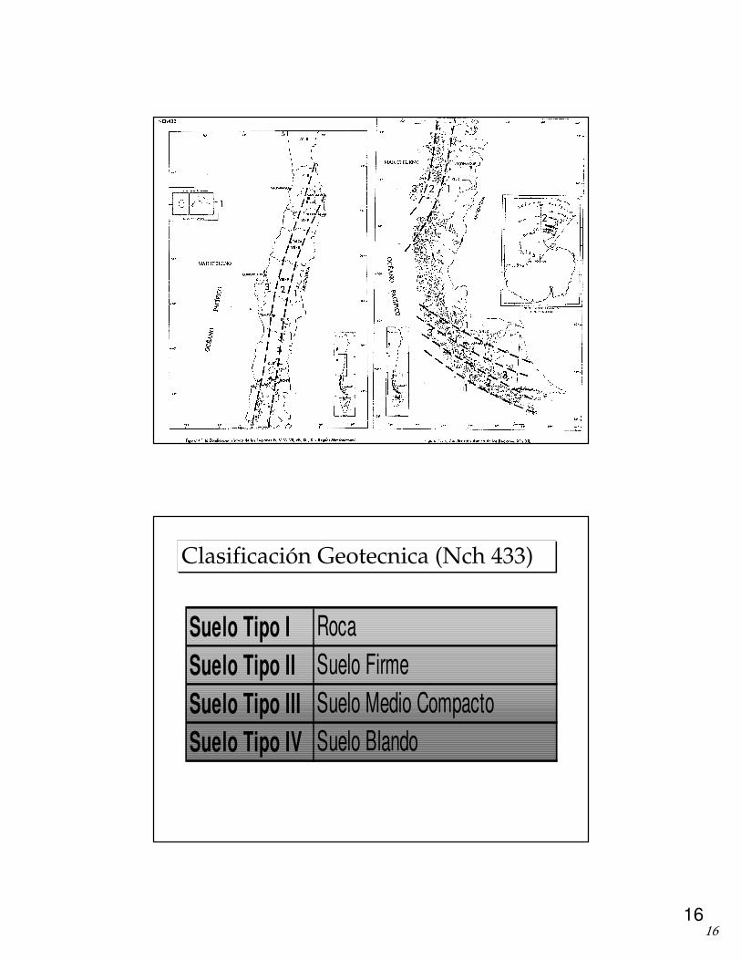
Zonificación Geotécnica de Chile (Nch 433)

1616

Clasificación Geotecnica (Nch 433)

Suelo Tipo I RocaSuelo Tipo II Suelo FirmeSuelo Tipo III Suelo Medio CompactoSuelo Tipo IV Suelo Blando

1919

Ao = aceleración efectiva máxima del suelo

Suelo CrDuros, Densos 0,45Suelos o Blandos 0,70Rellenos sueltos 0,58

Categoría del edificio IA 1.2B 1.2C 1.0D 1.6

��

Zona sísimica Ao1 0,20 g2 0,30 g3 0,40 g

��

2020

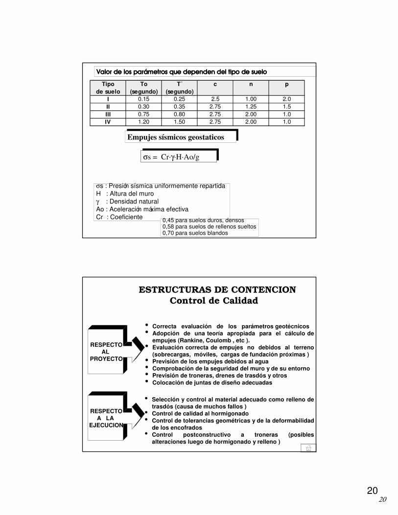
Tipo To T´ c n pde suelo (segundo) (segundo)

I 0.15 0.25 2.5 1.00 2.0II 0.30 0.35 2.75 1.25 1.5III 0.75 0.80 2.75 2.00 1.0IV 1.20 1.50 2.75 2.00 1.0

��

Empujes sísmicos geostaticos

σs = Cr·γ·H·Ao/g

σs : Presión sísmica uniformemente repartidaH : Altura del muroγ : Densidad naturalAo : Aceleración máxima efectivaCr : Coeficiente 0,45 para suelos duros, densos

0,58 para suelos de rellenos sueltos0,70 para suelos blandos

ESTRUCTURAS DE CONTENCIONControl de Calidad

RESPECTOAL

PROYECTO

• Correcta evaluación de los parámetros geotécnicos• Adopción de una teoría apropiada para el cálculo de

empujes (Rankine, Coulomb , etc ).• Evaluación correcta de empujes no debidos al terreno

(sobrecargas, móviles, cargas de fundación próximas )• Previsión de los empujes debidos al agua• Comprobación de la seguridad del muro y de su entorno• Previsión de troneras, drenes de trasdós y otros• Colocación de juntas de diseño adecuadas

RESPECTOA LA

EJECUCION

• Selección y control al material adecuado como relleno de trasdós (causa de muchos fallos )

• Control de calidad al hormigonado• Control de tolerancias geométricas y de la deformabilidad

de los encofrados• Control postconstructivo a troneras (posibles

alteraciones luego de hormigonado y relleno )

2121

��

��

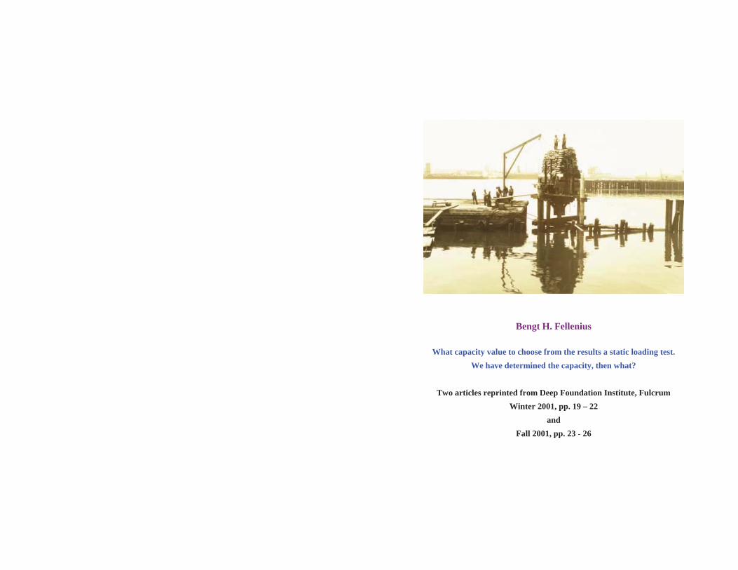
Bengt H. Fellenius

What capacity value to choose from the results a static loading test. We have determined the capacity, then what?

Two articles reprinted from Deep Foundation Institute, Fulcrum Winter 2001, pp. 19 – 22

andFall 2001, pp. 23 - 26

What Capacity Value to Choose from the Results a Static Loading Test Bengt H. Fellenius, Dr.Tech., P.Eng.

1. IntroductionFor pile foundation projects, it is usually necessary to confirm capacity and to verify that the behavior of the piles agrees with the assumptions of the design. Frequently, this is achieved by means of performing a static loading test, and, normally, determining the capacity is the primary purpose of the test. The capacity can, crudely, be defined as the load for which rapid movement occurs under sustained or slight increase of the applied load⎯the pile plunges. This definition is inadequate, however, because large movements are required for a pile to reach plunging mode and large movements are often governed less by the capacity of the pile-soil system and more by the capacity of the man at the pump. On most occasions, a distinct plunging ultimate load is not obtained in the test and, therefore, the pile capacity or ultimate load must be determined by some definition based on the load-movement data recorded in the test.

An old definition of capacity has been the load for which the pile head movement exceeds a certain value, usually 10 % of the diameter of the pile, or a given distance, often 1.5 inch. Such definitions do not consider the elastic shortening of the pile, which can be substantial for long piles, while it is negligible for short piles. In reality, a movement limit relates only to a movement allowed by the superstructure to be supported by the pile, and it does not relate to the capacity of the pile in the static loading test. As such, the 10 % or any other ratio to the pile diameter is meaningless from both the point-of-view of the pile-soil behavior and the structure. Similarly, 1.5-inch maximum movement criterion can be just right for the structure, but it has nothing to do with the pile-soil behavior. The question could be “Should the definition consider the structure that is going to be supported by the pile“?

For now, let’s restrict ourselves to a definition of capacity in the geotechnical sense of the word. Sometimes, the pile capacity is defined as the load at the intersection of two straight lines, approximating an initial pseudo-elastic portion of the curve and a final pseudo-plastic portion. This definition results in interpreted capacity values, which depend greatly on conjecture and on the scale of the graph. Change the scales and the perceived capacity value changes also. A

loading test is influenced by many occurrences, but the draughting manner should not be one of these.

Without a proper definition, capacity interpretation becomes meaningless for cases where obvious plunging has not occurred. To be “proper”, a definition of pile capacity must be based on a mathematical rule and generate a repeatable value that is independent of scale relations and eye-balling ability of the interpreter.

There is more to a static loading test than analysis of data obtained. As a minimum requirement, the test should be performed in accordance with the ASTM guidelines (D 1143 and D 3689) for axial loading (compression and tension, respectively), keeping in mind that the guidelines refer to routine testing. Tests involving instrumented piles may well need stricter performance rules.

Some time ago, the author presented nine different definitions of pile capacity evaluated from load-movement records of a static loading test (Fellenius, 1975; 1980). Four of these have particular interest, namely, the Davisson Offset Limit, the DeBeer Yield Limit, the Hansen Ultimate Load, and the Chin-Kondner Extrapolation. Recently, a fifth method was proposed by Luciano Decourt in Brazil (Decourt, 1999). The methods, including the Decourt Extrapolation are presented in the following.

2. The Davisson Offset Limit Load The Offset Limit Method is probably the best known and widely used method in North America. The method was proposed by Davisson (1972) as the load corresponding to the movement that exceeds the elastic compression of the pile (taken as a free-standing column) by a value of 0.15 inch (4 mm) plus a factor equal to the diameter of the pile divided by 120. Fig. 1 shows an example of a load-movement diagram from a static loading test on a 12-inch precast concrete pile. (The method of testing this pile is the constant-rate-of-penetration method, which is why the load-movement curve shows so many plotted points). The Davisson limit load is added to the curve presented in Fig. 1. For the 12-inch diameter example pile, the offset value is 0.25 inch (6 mm) and the Load Limit is 375 kips.

Notice that the Offset Limit Load is not necessarily the ultimate load. The method is based on the assumption that capacity is reached at a certain small toe movement and tries to estimate that movement by compensating for the stiffness (length and diameter) of the pile. It was developed by correlating—to one single criterion—a large number subjectively determined pile capacities for a data base of pile loading tests. It is primarily intended for test results from driven piles tested according to quick methods and it has gained a widespread use in phase with the increasing popularity of wave equation analysis of driven piles and dynamic testing.

Fig. 1 The Offset Limit Method

3. De Beer Yield LoadIf a trend is difficult to discern when analyzing data, a well known trick is to plot the data to logarithmic scale rather than to linear scale. Then, provided the data spread is an order of magnitude or two, all relations become more or less linear. (Determining the slope and location of the line and using this for some mathematical truths is rarely advisable; the linearity has more the effect of hiding details than revealing them). DeBeer (1968) made use of the logarithmic linearity by plotting the load-movement data in a double-logarithmic diagram as shown in Fig. 2.

Fig. 2 DeBeer’s Double-Logarithmic Method

If the ultimate load was reached in the test, two line approximations will appear; one before and one after the ultimate load (provided the number of points allow the linear trend to develop). The slopes are meaningless, but the intersection of the lines is useful as it indicates where a change occurs in the response of the piles to the applied load. DeBeer called the intersection the Yield Load. It occurs at a load of 360 kips for the example.

4. The Hansen 80-% Criterion

J. Brinch Hansen (1963) proposed a definition for pile capacity as the load that gives four times the movement of the pile head as obtained for 80 % of that load. This ‘80%- criterion’ can be estimated directly from the load-movement curve, but it is more accurately determined in a plot of the square root of each movement value divided by its load value and plotted against the movement.

Normally, the 80%-criterion agrees well with the intuitively perceived “plunging failure” of the pile. The following simple relations can be derived for computing the capacity or ultimate resistance, Qu, according to the Hansen 80%-criterion for the Ultimate Load:

(1)212

1CC

Qu =

(2) 1

2

CC

u =δ

Where Qu = capacity or ultimate load δu = movement at the ultimate load

C1 = slope of the straight line C2 = y-intercept of the straight line

The Hansen method is applied to the example case, as illustrated in Fig. 3. Eq. 1 indicates that the Hansen Ultimate Load is 418 kips, a value slightly smaller than the 440-kip maximum test load applied to the pile head.

The 80-% criterion determines the load-movement curve for which the Hansen plot is a straight line throughout. The equation for this ‘ideal’ curve is shown as a dashed line in Fig. 3 and Eq. 3 gives the relation for the curve.

Page 9

Fig. 4 presents a diagram over shaft resistance versus relative movement between the pile shaft and the soil that is a bit more complex, but more realistic: The soil response demonstrates a strain-softening response after the resistance having reached a peak value: the shear resistance drops off to about 80 % of the peak value. This is more representative for the behavior of a pile shaft sliding past the soil. The test results for this shaft resistance are shown in Fig. 5.

Fig. 4 Percent shaft resistance as a function of relative movement between pile shaft and a strain-softening soil

Fig. 5 The effect of strain-softening shaft resistance

As shown in Fig. 5, because of the effect of the strain softening, the evaluated Offset Limit has diminished.

Adding the effect of varying degree of residual load in the pile, will affect the test evaluation in a similar manner as for the first case.

Were any of the other methods of determining the “Failure Load” used as reference instead of the Offset Limit Load, the results would be similar.

3. Conclusions

The result of a static loading test does not provide the simple answers one at first may think. First, there is a considerable variation in the methods of “Failure Load” interpretation used in the industry. Then, the effect of residual load and varying degree of strain-softening will appreciably affect the interpretation. Indeed, a static test that measures only the applied load and the pile head movement is a very crude test. For small and non-complex projects, such level of sophistication, or lack thereof, is acceptable if the uncertainty is covered by a judiciously large factor of safety. For larger projects, however, this approach is costly. For these, the test pile should be instrumented and the test data evaluated carefully to work out the various influencing factors. For projects involving many piles, several test piles may be desirable, though this could be prohibitively costly. If so, combining an instrumented static loading test with dynamic testing, which can be performed on many piles at a relatively small cost, can extend the application of the more detailed results of the instrumented static test.

The potential presence of residual load and its varying magnitude makes methods of interpretation based on initial and final slopes of the load-movement curve somewhat illogical.

Design of piles should be less based on the capacity value and more emphasize the settlement of the pile under sustained load. It will then be easier and more logical to incorporate aspects such as downdrag and dragload into the design.

References

Fellenius, B. H., 1984. Ignorance is bliss - And that is why we sleep so well. Geotechnical News, Vol. 2, No. 4, pp. 14 - 15.

Fellenius B. H., 1999. Bearing capacity — A delusion? Proceedings of the Deep Foundation Institute 1999 Annual Meeting, Dearborn, Michigan, October 14 -16, 1999.

0

25

50

75

100

125

0 5 10 15 20 25

MOVEMENT (mm)

MO

BIL

IZED

RES

ISTA

NC

E (%

)

0

200

400

600

800

1,000

1,200

0 5 10 15 20 25

MOVEMENT (mm)

LOAD

(K

N)

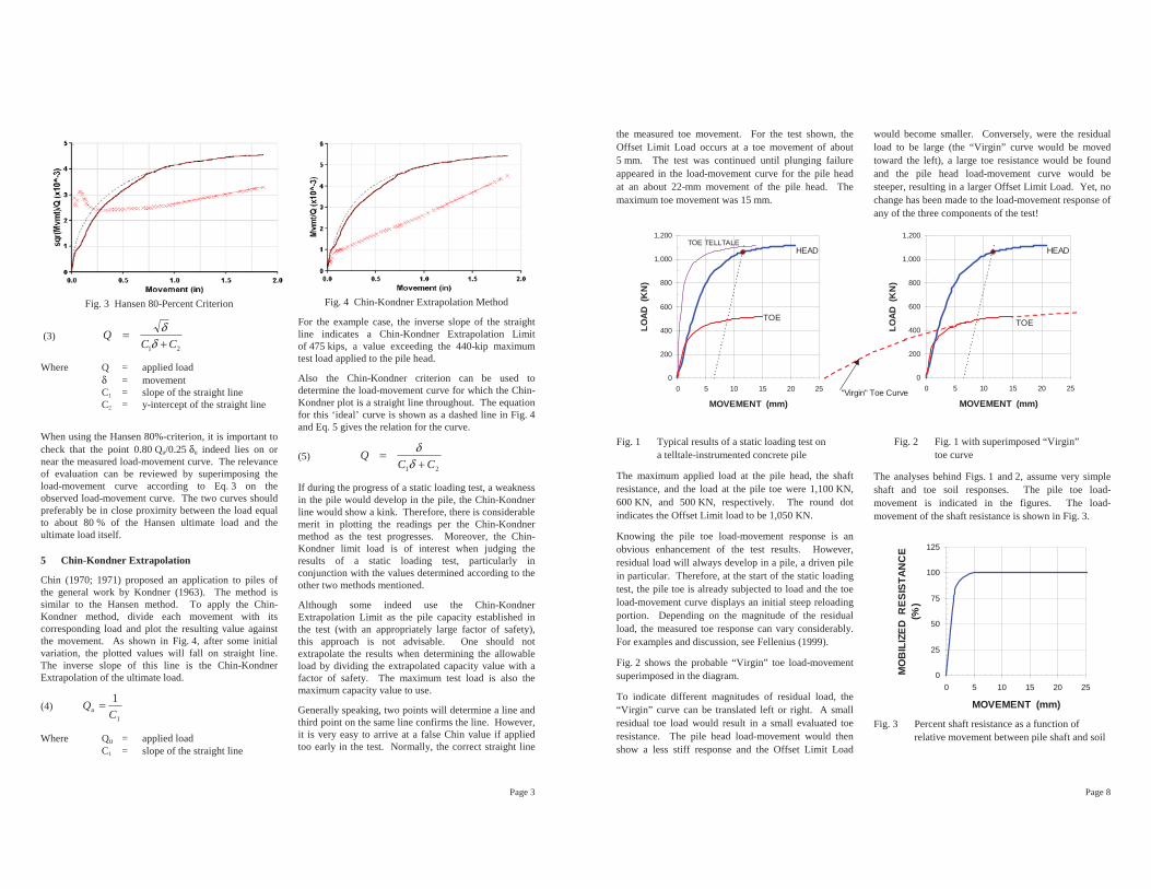
the measured toe movement. For the test shown, the Offset Limit Load occurs at a toe movement of about 5 mm. The test was continued until plunging failure appeared in the load-movement curve for the pile head at an about 22-mm movement of the pile head. The maximum toe movement was 15 mm.

Fig. 1 Typical results of a static loading test on a telltale-instrumented concrete pile

The maximum applied load at the pile head, the shaft resistance, and the load at the pile toe were 1,100 KN,600 KN, and 500 KN, respectively. The round dot indicates the Offset Limit load to be 1,050 KN.

Knowing the pile toe load-movement response is an obvious enhancement of the test results. However, residual load will always develop in a pile, a driven pile in particular. Therefore, at the start of the static loading test, the pile toe is already subjected to load and the toe load-movement curve displays an initial steep reloading portion. Depending on the magnitude of the residual load, the measured toe response can vary considerably. For examples and discussion, see Fellenius (1999).

Fig. 2 shows the probable “Virgin” toe load-movement superimposed in the diagram.

To indicate different magnitudes of residual load, the “Virgin” curve can be translated left or right. A small residual toe load would result in a small evaluated toe resistance. The pile head load-movement would then show a less stiff response and the Offset Limit Load

would become smaller. Conversely, were the residual load to be large (the “Virgin” curve would be moved toward the left), a large toe resistance would be found and the pile head load-movement curve would be steeper, resulting in a larger Offset Limit Load. Yet, no change has been made to the load-movement response of any of the three components of the test!

Fig. 2 Fig. 1 with superimposed “Virgin” toe curve

The analyses behind Figs. 1 and 2, assume very simple shaft and toe soil responses. The pile toe load-movement is indicated in the figures. The load-movement of the shaft resistance is shown in Fig. 3.

Fig. 3 Percent shaft resistance as a function of relative movement between pile shaft and soil

0

25

50

75

100

125

0 5 10 15 20 25

MOVEMENT (mm)

MO

BIL

IZED

RES

ISTA

NC

E (%

)

0

200

400

600

800

1,000

1,200

0 5 10 15 20 25

MOVEMENT (mm)

LOAD

(K

N)

HEAD

TOE

TOE TELLTALE

0

200

400

600

800

1,000

1,200

0 5 10 15 20 25

MOVEMENT (mm)

LOAD

(K

N)

HEAD

"Virgin" Toe Curve

TOE

Page 3

Fig. 3 Hansen 80-Percent Criterion

(3) 21 CC

Q+

=δ

δ

Where Q = applied load δ = movement

C1 = slope of the straight line C2 = y-intercept of the straight line

When using the Hansen 80%-criterion, it is important to check that the point 0.80 Qu/0.25 δu indeed lies on or near the measured load-movement curve. The relevance of evaluation can be reviewed by superimposing the load-movement curve according to Eq. 3 on the observed load-movement curve. The two curves should preferably be in close proximity between the load equal to about 80 % of the Hansen ultimate load and the ultimate load itself.

5 Chin-Kondner Extrapolation

Chin (1970; 1971) proposed an application to piles of the general work by Kondner (1963). The method is similar to the Hansen method. To apply the Chin-Kondner method, divide each movement with its corresponding load and plot the resulting value against the movement. As shown in Fig. 4, after some initial variation, the plotted values will fall on straight line. The inverse slope of this line is the Chin-Kondner Extrapolation of the ultimate load.

(4)1

1C

Qu =

Where Qu = applied load C1 = slope of the straight line

Fig. 4 Chin-Kondner Extrapolation Method

For the example case, the inverse slope of the straight line indicates a Chin-Kondner Extrapolation Limit of 475 kips, a value exceeding the 440-kip maximum test load applied to the pile head.

Also the Chin-Kondner criterion can be used to determine the load-movement curve for which the Chin-Kondner plot is a straight line throughout. The equation for this ‘ideal’ curve is shown as a dashed line in Fig. 4 and Eq. 5 gives the relation for the curve.

(5) 21 CC

Q+

=δ

δ

If during the progress of a static loading test, a weakness in the pile would develop in the pile, the Chin-Kondner line would show a kink. Therefore, there is considerable merit in plotting the readings per the Chin-Kondner method as the test progresses. Moreover, the Chin-Kondner limit load is of interest when judging the results of a static loading test, particularly in conjunction with the values determined according to the other two methods mentioned.

Although some indeed use the Chin-Kondner Extrapolation Limit as the pile capacity established in the test (with an appropriately large factor of safety), this approach is not advisable. One should not extrapolate the results when determining the allowable load by dividing the extrapolated capacity value with a factor of safety. The maximum test load is also the maximum capacity value to use.

Generally speaking, two points will determine a line and third point on the same line confirms the line. However, it is very easy to arrive at a false Chin value if applied too early in the test. Normally, the correct straight line

does not start to materialize until the test load has passed the Davisson Offset Limit. As an approximate rule, the Chin-Kondner Extrapolation load is about 20 % to 40 % greater than the Davisson limit. When this is not a case, it is advisable to take a closer look at all the test data.

The Chin method is applicable on both quick and slow tests, provided constant time increments are used. The ASTM "standard method" is therefore usually not applicable. Also, the number of monitored values are too few in the "standard test"; the interesting development could well appear between the seventh and eighth load increments and be lost.

4 Decourt Extrapolation

Decourt (1999) proposes a method, which construction is similar to those used in Chin-Kondner and Hansen methods. To apply the method, divide each load with its corresponding movement and plot the resulting value against the applied load. The left side diagram in Fig. 5 shows the results: a curve that tends to a line that intersects with the abscissa. A linear regression over the apparent line (last five points in the example case) determines the line. The Decourt extrapolation load limit is the value of load at the intersection, 474 kips in the example case. As shown in the right side diagram of Fig. 4, similarly to the Chin-Kondner and Hansen methods, an ‘ideal’ curve can be calculated and compared to the actual load-movement curve of the test.

The Decourt extrapolation load limit is equal to the ratio between the y-intercept and the slope of the line as given in Eq. 6.

(6) 1

2

CC

Qu =

The equation of the ‘ideal’ curve is given in Eq. 7.

(7) δ

δ1

2

1 CC

Q−

=

Where Qu = capacity or ultimate load Q = applied load

δ = movement C1 = slope of the straight line C2 = y-intercept of the straight line

Results from using the Decourt method are very similar to those of the Chin-Kondner method. The Decourt method has the advantage that a plot prepared while the static loading test is in progress will allow the User to ‘eyeball’ the projected capacity directly once a straight-line plot starts to develop.

0 100 200 300 400 5000

500,000

1,000,000

1,500,000

2,000,000

LOAD (kips)

LOAD

/MVM

NT

-- Q

/s (

inch

/kip

s)

Ult.Res = 474 kips

Linear Regression Line

0.0 0.5 1.0 1.5 2.00

100

200

300

400

500

MOVEMENT (inches)

LOAD

(ki

ps)

Fig. 5 Decourt Extrapolation Method

Page 7

always is to be coupled with a serviceability limit state design, the pile capacity should be determined by a method closer to the plunging limit load, that is, the Brinch-Hansen 80 %-criterion is preferred over the Offset Limit Load).

2. Choice of Evaluation Method

It is difficult to make a rational choice of the best capacity criterion to use, because the preferred criterion depends heavily on one's past experience and conception of what constitutes the ultimate resistance of a pile.

The Davisson Offset Limit is very sensitive to errors in the measurements of load and movement and requires well maintained equipment and accurate measurements. (No static loading test should rely on the jack pressure for determining the applied load. A load-cell must be used at all times. For a case in point, see Fellenius, 1984). In a sense, the Offset Limit is a modification of the "gross movement" criterion of the past (which used to be 1.5 inch movement at the maximum load). Actually, the Offset-Limit method is an empirical method that does not really consider the actual transfer of the applied load to the soil. However, it is easy to apply and has gained a wide acceptance.

The Davisson Offset Limit offers the benefit of allowing the engineer, when proof testing a pile for a certain allowable load, to determine in advance the maximum allowable movement for this load with consideration of the length and size of the pile. Thus, contract specifications can be drawn up including an acceptance criterion for piles proof tested according to quick testing methods. The specifications can simply call for a test to at least twice the design load, as usual, and declare that at a test load equal to a factor, F, times the design load, the movement shall be smaller than the elastic column compression of the pile, plus 0.15 inch (4 mm), plus a value equal to the diameter divided by 120. The factor F is a safety factor and should be chosen according to circumstances in each case. The usual range is 1.8 through 2.0.

The Brinch-Hansen 80%-criterion usually gives a Qu-value, which is close to what one subjectively accepts as the true ultimate resistance determined from the results of the static loading test. The value is smaller than the Chin-Kondner value. Note, however, that the

Brinch-Hansen method is more sensitive to inaccuracies of the test data than is the Chin-Kondner method. The usual range is 2.0 through 2.5. The Chin-Kondner Extrapolation and the Decourt Extrapolation limit load values are approached asymptotically. Therefore, the these two methods are always obtained by extrapolation. It is a sound engineering rule never to interpret the results from a static loading test to obtain an ultimate load larger than the maximum load applied to the pile in the test. For this reason, an allowable load cannot, must not, be determined by dividing the limit loads according to Chin-Kondner and Decourt methods with a factor of safety.

The Brinch Hansen's 80%-criterion and the Chin and Decourt extrapolation methods allow the later part of the load-movement be continued beyond the maximum load applied, extrapolating the curve. This is very tempting. That is, it is easy to fool oneself and believe that the extrapolated part of the curve is as true as the measured.

2. Bearing Capacity Is No Simple Matter

The load-movement consists of three components: the load-movement of the shaft resistance, the compression of the pile, and the load-movement of the pile toe. The combined load-movement response to a load applied to a pile head therefore reflects the relative magnitude of the three. Moreover, only the shaft resistance exhibits an ultimate resistance. The compression of the pile is really a more or less linear response to the applied load and does not have an ultimate value (disregarding a structural failure when the load reaches the strength of the pile material). However, the load-movement of the pile toe is also a more or less linear response to the load that has no failure value. Therefore, the concept of an ultimate load, a failure load or capacity is really a fallacy and a design based on the ultimate load is a quasi concept, and of uncertain relevance for the assessment of a pile.

The statement is illustrated in Fig. 1, which presents the results from a typical test on a 15 m long, 300 mm diameter, driven concrete pile.

The figure includes the load-movement of the pile toe, measured, say, by a strain gage or a load cell at the pile toe and a toe telltale. The load-movement is shown both as the applied load and as actual toe resistance versus

We have determined the capacity, then what? Bengt H. Fellenius, Dr.Tech., P.Eng.

Summary The purpose of the static loading test is to find the allowable load, which is established by dividing the capacity with a factor of safety. The factor of safety normally applied in the industry ranges from a low of 1.8 through a high of 2.5,depending on several reasons, not least the method used to determine the pile capacity from the load-movement curve. However, the concept of ultimate load, failure load, or capacity is really a fallacy. A design based on the ultimate load is aquasi concept and of ambiguous relevance for the assessment of a pile. This because the pile-head load-movement curve is the combined effect of the load-movement to failure of the shaft resistance, the elastic compression of the pile itself, and theload-movement of the pile toe. Of the three, failure only develops for the first component. Even for a test where a plunging failure appears, the plunging is a combination of reduced shaft resistance due to strain-softening, shortening of the pile and residual load at the pile toe at the start of the test. Pile design should emphasize settlement analysis and give less weight to the capacity of the pile.

1. Factor of Safety

The capacity of a pile is the ultimate soil resistance of the pile determined from the load-movement behavior measured in the static loading test. But the purpose of the test is, knowing the capacity, to find a safe load that can be supported on the pile, which load is called the allowable load. The allowable load is established by dividing the capacity by a factor of safety.

The factor of safety is not a singular value applicable at all times. Its value depends on the desired freedom from unacceptable consequence of a failure, as well as on the level of knowledge and control of the aspects influencing the variation of capacity at the site. Not least important are, one, the method used to determine or define the ultimate load from the test results and, two,how representative the test is for the piles at the site. Most codes specify a single factor regardless of conditions, usually 2.0, frequently larger.

Where some freedom is granted the design engineer, practice has developed toward using a range of factors of safety, as follows. In a testing programme performed early in the design work and testing piles which are not necessarily the same type, size, or length as those which will be used for the final project, the safety factor applied is high, usually 2.5, to account for the unknowns. In the case of testing during a final design phase, when the loading test occurs under conditions well representative for the project, the safety factor could be reduced to 2.2. When a test is performed for purpose of verifying the final design, testing a pile that is installed by the actual piling contractor and intended

for the actual project, the factor commonly applied is 2.0. Well into the project, when testing is carried out for purpose of proof testing and conditions are favorable, the factor may sometimes be further reduced and become 1.8. Reduction of the safety factor may also be warranted when limited variability is confirmed by means of combining the design with detailed site investigation and control procedures of high quality. One must also consider the number of tests performed and the scatter of results. The applied factor of safety can often be reduced due to the assurance gained for driven piles by means of incorporating dynamic methods for controlling hammer performance and for capacity determination.

The value of the factor of safety to apply depends on the method used to determine the capacity. A conservative method, such as the Davisson Offset Limit Load, warrants the use of a smaller factor as opposed to a “liberal” method, such as the Brinch Hansen 80%-criterion. It is good practice to apply more than one method for defining the capacity and to apply to each method its own factor of safety letting the smallest allowable load govern the design.

Lately, the industry is required to evaluate the results of a static loading test according to Load-and-Resistance-Factor-Design, LRFD. The principle of the LRFD is simple. A “resistance factor” is applied to the capacity and a “load factor” is applied to the load. A load factor and a resistance factor specified to 1.4 and 0.6 “calibrate” to a conventional factor-of-safety, (“global factor”) of 1.4÷0.6 = 2.33. (When considering that factored design is an ultimate limit state design that

Page 5

5. References Davisson, M. T., 1972. High capacity piles. Proceedings of Lecture Series on Innovations in Foundation Construction, American Society of Civil Engineers, ASCE, Illinois Section, Chicago, March 22, pp. 81 - 112. DeBeer, E. E., 1968. Proefondervindlijke bijdrage tot de studie van het grensdraag vermogen van zand onder funderingen op staal. Tijdshift der Openbar Verken van Belgie, No. 6, 1967 and No. 4, 5, and 6, 1968. Decourt, L., 1999. Behavior of foundations under working load conditions. Proceedings of the 11th Pan-American Conference on Soil Mechanics and Geotechnical Engineering, Foz DoIguassu, Brazil, August 1999, Vol. 4, pp. 453 - 488. Fellenius B. H., 1975. Test loading of piles. Methods, interpretation, and new proof testing procedure. ASCE, Vol. 101, GT9, pp. 855 - 869. Fellenius B. H., 1980. The analysis of results from routine pile loading tests. Ground Engineering, London, Vol. 13, No. 6, pp. 19 - 31. Hansen, J.B., 1963. Discussion on hyperbolic stress-strain response. Cohesive soils. American Society of Civil Engineers, ASCE, Journal for Soil Mechanics and Foundation Engineering, Vol. 89, SM4, pp. 241 - 242.

geotecnia

Documents