documentos de trabajo n.º 1301 - banco de españa€¦ · los precios se determinan por un logit...
TRANSCRIPT

LOGIT PRICE DYNAMICS
James Costain and Anton Nakov
Documentos de Trabajo N.º 1301
2013

LOGIT PRICE DYNAMICS

Documentos de Trabajo. N.º 1301
2013
James Costain and Anton Nakov
BANCO DE ESPAÑA
LOGIT PRICE DYNAMICS

The Working Paper Series seeks to disseminate original research in economics and fi nance. All papers have been anonymously refereed. By publishing these papers, the Banco de España aims to contribute to economic analysis and, in particular, to knowledge of the Spanish economy and its international environment.
The opinions and analyses in the Working Paper Series are the responsibility of the authors and, therefore, do not necessarily coincide with those of the Banco de España or the Eurosystem.
The Banco de España disseminates its main reports and most of its publications via the INTERNET at the following website: http://www.bde.es.
Reproduction for educational and non-commercial purposes is permitted provided that the source is acknowledged.
© BANCO DE ESPAÑA, Madrid, 2013
ISSN: 1579-8666 (on line)

Abstract
We propose a near-rational model of retail price adjustment consistent with microeconomic
and macroeconomic evidence on price dynamics. Our framework is based on the idea
that avoiding errors in decision making is costly. Given our assumed cost function for error
avoidance, the timing of fi rms’ price adjustments is determined by a weighted binary logit,
and the prices they choose are determined by a multinomial logit. We build this behavior into
a DSGE model, estimate the decision cost function by matching microdata, and simulate
aggregate dynamics using a tractable algorithm for heterogeneous-agent models. Both
errors in the prices fi rms set, and errors in the timing of these adjustments, are relevant
for our results. Errors of the fi rst type help make our model consistent with some puzzling
observations from microdata, such as the coexistence of large and small price changes, the
behavior of adjustment hazards, and the relative variability of prices and costs. Errors of
the second type increase the real effects of monetary shocks, by reducing the correlation
between the value of price adjustment and the probability of adjustment, (i.e., by reducing
the «selection effect»). Allowing for both types of errors also helps reproduce the effects
of trend infl ation on price adjustment behavior. Our model of error-prone pricing in many
ways resembles a stochastic menu cost (SMC) model, but it has less free parameters
than most SMC models have, and unlike those models, it does not require the implausible
assumption of i.i.d. adjustment costs. Our derivation of a weighted logit from control costs
oers an alternative justication for the adjustment hazard derived by Woodford (2008). Our
assumption that costs are related to entropy is similar to the framework of Sims (2003) and
the subsequent «rational inattention» literature. However, our setup has the major technical
advantage that a fi rm’s idiosyncratic state variable is simply its price level and productivity,
whereas under rational inattention a fi rm’s idiosyncratic state is its prior (which is generally an
infi nite-dimensional object).
Keywords: nominal rigidity, logit equilibrium, state-dependent pricing, near rationality,
information-constrained pricing.
JEL classifi cation: E31, D81, C72.

Resumen
Proponemos un modelo cuasi racional de ajustes de precios en el mercado minorista
que es coherente con la evidencia micro y macro de la dinámica de los precios. Nuestro
marco está basado en la idea de que evitar errores en las decisiones implica un coste.
Dada la asumida función del coste de evitar errores, los momentos escogidos para cambiar
los precios se determinan por un logit binario ponderado, mientras que los precios escogidos
se determinan por un logit multinomio. Incorporamos este comportamiento en un modelo
DSGE, estimamos la función de costes de decisión ajustando los datos micro y simulamos la
dinámica agregada utilizando un algoritmo manejable de agentes heterogeneos.
Tanto los errores en los precios que establecen las empresas como los errores en los
momentos escogidos para cambiar son relevantes para nuestros resultados. Los errores del
primer tipo ayudan al modelo a reproducir algunas observaciones sorprendentes de los datos
micro, como la coexistencia de cambios de precios pequeños y grandes, el comportamiento
de la probabilidad de ajuste en función de la edad de los precios, y la variabilidad relativa de
los precios y los costes. Los errores del segundo tipo aumentan los efectos reales de shocks
monetarios, reduciendo la correlación entre el valor de ajustar y la probabilidad de ajuste (es
decir, reduciendo el «efecto de selección»). Permitir ambos tipos de errores también ayuda
a reproducir los efectos de la infl ación sobre el comportamiento del ajuste de los precios.
Nuestro modelo de fi jación de precios sujeto a errores se parece en muchos aspectos al
modelo de costes de menú estocásticos (CME), pero tiene menos parámetros libres que
la mayoría de los modelos CME y, a diferencia de estos modelos, no requiere el supuesto
implausible de que los costes de menú estén distribuidos idénticamente y de manera
independiente. Nuestra derivación de un logit ponderado basado en costes de control ofrece
una justifi cación alternativa al modelo de ajuste de Woodford (2008). Nuestro supuesto de
que los costes están relacionados con la entropía es similar al marco de Sims (2003) y a la
literatura posterior sobre «falta de atención racional». No obstante, nuestro modelo tiene
la principal ventaja de que la variable de estado idiosincrática de la empresa incluye solo su
precio y productividad, mientras que en el modelo de «falta de atención racional» la variable de
estado idiosincrática incluye el prior de la empresa (en general, un objeto de dimensión infi nita).
Palabras clave: nominal, equilibrio logit, fi jación de precios dependiente del estado, cuasi
racionalidad, fi jación de precios con información restringida.
Códigos JEL: E31, D81, C72.

BANCO DE ESPAÑA 7 DOCUMENTO DE TRABAJO N.º 1301
1 Introduction1
Economists seeking to explain price stickiness have often appealed to small fixed costs of nom-inal price changes, commonly called “menu costs” (Barro 1972). If shocks to fundamentalsaccumulate relatively slowly, then even small menu costs might suffice to make price adjust-ments infrequent and to make aggregate dynamics deviate in a nontrivial way from the flexible-price optimum (Mankiw 1985). However, Golosov and Lucas (2007) showed quantitatively, ina macroeconomic model with realistically large firm-specific shocks, that fixed menu costs dolittle to generate aggregate price stickiness. The dynamics of their model are quite close tomonetary neutrality, so fixed menu costs do not seem promising to explain the substantial realeffects of monetary shocks observed in macroeconomic data (e.g. Christiano, Eichenbaum, andEvans, 1999). Moreover, detailed microeconomic evidence suggests that menu costs, as usuallyinterpreted, are only a small fraction of the overall costs of price setting (Zbaracki et al. 2004).A much larger part of the costs of price adjustment consists of managerial costs associated withinformation collection and decision making. This raises the question: can costs related to deci-sion making explain microeconomic and macroeconomic evidence of price stickiness better thanfixed menu costs do? And furthermore, how exactly should these costs be modeled?
This paper proposes a simple model of price stickiness based on costly decision-making,estimates its two free parameters, and shows by simulation that it is consistent with a widevariety of microeconomic and macroeconomic evidence. Our setup is motivated by two keyconsiderations. First, if choice is costly, then decisions will typically be imperfect, that is,prone to errors. Thus it is natural to think of the outcomes of decisions as random variables,rather than treating the action taken as a deterministic function of fundamentals. Second, it isnatural to assume that more precise decisions are more costly than imprecise ones. Motivatedby these points, we adopt the “control cost” approach from game theory (see, for example,van Damme 1991). Formally, instead of modeling the choice of an optimal action directly, thisapproach defines the decision problem as the choice of a probability distribution over possibleactions. The problem is solved subject to a cost function with the property that more precisedecisions (more concentrated distributions) are more costly. Making any given decision in aperfectly precise way is feasible, but this is usually not worth the cost. Therefore the actionactually taken will be a random variable correlated with fundamentals, instead of depending onfundamentals in a deterministic way.
In the context of dynamic price setting, a firm faces two key margins of decision: when tochange the price of a product it sells, and what new price to set. We allow for errors on boththese margins. The exact shape of the error distribution depends on the assumed form of the costfunction for precision. It happens to be particularly convenient to measure precision in termsof entropy, and to define costs as a linear function of the relative entropy of the distribution ofactions, as compared with a uniform distribution. Under these functional forms, the distributionof actions is a multinomial logit. This implies that the probability of taking any given action isa smoothly increasing function of the value of that action, compared with the values of other
1We thank Herve Le Bihan, Anton Cheremukhin, Bartosz Mackowiak, Filip Matejka, Galo Nuno, AntonellaTutino, Carl Walsh, Mirko Wiederholt, Michael Woodford, and seminar participants at UC Santa Cruz, the Bankof Spain, T2M 2012, ESSIM 2012, CEF 2012, and EEA-ESEM 2012 for helpful comments. We are especiallygrateful to Virgiliu Midrigan for making the Dominick’s price data available to us, and to the James M. KiltsCenter at the Univ. of Chicago GSB, which is the original source of the data. Views expressed here are those ofthe authors and do not necessarily coincide with those of the Bank of Spain or the Eurosystem.

BANCO DE ESPAÑA 8 DOCUMENTO DE TRABAJO N.º 1301
feasible actions. General equilibrium then takes the form of a logit equilibrium:2 each decisionmaker plays a logit in which the values of actions are calculated under the assumption thatother decision makers play logits too. Backing out the costs associated with our benchmarkequilibrium, firms in our model spend roughly 0.9% of revenue on decision-making, and inaddition incur a loss of roughly 0.5% of revenue due to suboptimal choices.
The fact that an entropy-related cost function serves to “microfound” a logit distributionof actions has been shown by many previous authors in game theory and economics (Stahl1990; Marsili 1999; Mattson and Weibull 2002; Bono and Wolpert 2009; Matejka and McKay2011).3 However, economics applications have typically focused on decisions taken at known,exogenously given points in time; it is not immediately obvious how to apply the logit frameworkto a context like intermittent price adjustment where a key question is when adjustments shouldoccur. We study how the derivation of logit choice behavior can be extended so that it isapplicable to fully dynamic decisions of timing. We show that if the decision cost associatedwith an adjustment hazard is a linear function of its relative entropy, compared with a uniformadjustment hazard, then the decision of whether or not to adjust in a given time period takesthe form of a weighted binary logit. Stated differently, while a standard static logit model has asingle free parameter representing the accuracy of decisions, the weighted logit in our dynamicsetup has two free parameters, representing the speed and the accuracy of decision making.The inclusion of the speed parameter ensures that our model has a well-defined continuous-timelimit, and thus clarifies how parameters must be adjusted if the frequency of the data or themodel simulation is changed.
While it is reasonable to assume that the size and the timing of firms’ adjustments are bothsubject to error, we run simulations that shut down one type of mistakes or the other in orderto see what each one contributes to our model’s empirical performance. We find that errors inthe size of price changes help reproduce many phenomena observed in retail price microdatathat seem puzzling in the light of some standard models. In particular, unlike a fixed menu costmodel, our model implies that many large and small price changes coexist (Klenow and Kryvstov2008; Midrigan 2011; Klenow and Malin 2010, “Fact 7”). It implies that the probability of priceadjustment is nearly flat, but slightly decreasing in the first few months, as found in empiricalstudies that control for heterogeneity in adjustment frequency (Nakamura and Steinsson 2008,“Fact 5”; Klenow and Malin 2010, “Fact 10”). Furthermore, we find that the standard deviationof price adjustment is mostly constant, independent of the time since last adjustment (Klenowand Malin 2010, “Fact 10”). Most alternative models, including the Calvo model, instead implythat price adjustments are increasing in size. Also, our model implies that extremely high or lowprices are more likely to have been set recently than prices near the center of the distribution(Campbell and Eden 2010). Finally, prices are more volatile than costs, as documented byEichenbaum, Jaimovich, and Rebelo (2011), whereas the opposite is true both in the Calvomodel and the fixed menu cost model.
While errors in the size of price adjustments help reproduce patterns in microdata, by them-selves they do not imply strong real effects of monetary policy. Indeed, since the model witherrors only in the size of price adjustments has only one free parameter, it is hard to get it tomatch multiple features of the data simultaneously, and the degree of nonneutrality it implies
2Logit equilibrium is a commonly-applied parametric special case of quantal response equilibrium (see McK-elvey and Palfrey, 1995, 1998).
3This mathematical fact reflects much older results in physics, where a formally equivalent optimization prob-lem gives rise to the Boltzmann distribution of particles in a gas.

BANCO DE ESPAÑA 9 DOCUMENTO DE TRABAJO N.º 1301
is sensitive to the details of our calibration procedure. But whenever we include mistakes inthe timing of price adjustments, our model implies substantial monetary nonneutrality (roughlyhalfway between the effects observed in the fixed menu cost model, and the effects observedin the Calvo model). The cause of the nonneutrality is the same as in the Calvo model: bydecreasing the relation between the value of adjustment and the probability of adjustment, the“selection effect” highlighted by Caplin and Spulber (1987) and Golosov and Lucas (2007) isgreatly reduced. But in contrast with the Calvo setup, our model also does a good job in repro-ducing the effects of trend inflation on price adjustment. In particular, it is consistent with theeffect of trend inflation on the typical size of price changes, and on the fraction of adjustmentsthat are increases, which are both margins where the fixed menu cost model performs poorly.
1.1 Related literature
This paper has links to several areas of economic literature. A huge wave of recent researchhas documented the dynamics of price adjustment in new databases from the retail sector (keypapers include Klenow and Kryvtsov, 2008; Nakamura and Steinsson, 2008; and Klenow and Ma-lin, 2010; and Eichenbaum, Jaimovich, and Rebelo, 2011). In response, many macroeconomistshave simulated numerical models of pricing under fixed or stochastic menu costs in the pres-ence of aggregate and firm-specific shocks, fitting them to microdata and then studying theirmacroeconomic implications. Some influential papers in this tradition include Golosov and Lu-cas (2007), Midrigan (2011), Dotsey, King, and Wolman (2011), Alvarez, Beraja, Gonzalez, andNeumeyer (2011), Kehoe and Midrigan (2010), and Matejka (2011).4 A particularly promisingrecent branch of the literature instead considers both a fixed cost of price adjustment and a fixedcost of acquiring information (Alvarez, Lippi, and Paciello, 2011; Demery, 2012). Like our ownframework, these “menu cost and observation cost” models are highly empirically successful inspite of relying on only two free parameters to model the adjustment process.
While most recent work on state-dependent pricing assumes prices are set optimally subjectto menu costs, we assume instead that price adjustment involves errors, and we do not assumeany menu costs, at least not as they are usually interpreted. The fact that we allow for errorsmay seem like a radical break with standard practice in macroeconomics. But it is consistentwith microeconometrics, where error terms are indispensible (though they are not always in-terpreted as mistakes). In calibrating a representative-agent macroeconomic model, ignoringerrors is arguably consistent with microeconometric practice, since at least to a first approx-imation, errors may cancel out. But when calibrating a heterogeneous-agent macroeconomicmodel to the full distribution of adjustments in microdata, such an argument does not apply:if there are any errors at all, these are likely to increase the variance of observed adjustments,so that a calibration without errors would (for example) mistakenly overestimate the varianceof the underlying exogenous shocks. In this sense, the microdata-based calibration strategies inmost recent literature on state-dependent pricing may represent a more radical departure fromprevious microeconomic and macroeconomic methodology than our model does.
Our framework for modeling error-prone behavior, logit equilibrium, has been widely appliedin experimental game theory, where it has helped explain play in a number of games whereNash equilibrium performs poorly, such as the centipede game and Bertrand competition games
4This paper also builds on two related papers of our own: in Costain and Nakov (2011C) we study themicroeconomic and macroeconomic implications of logit errors in price decisions, while one specification consideredin Costain and Nakov (2011A) imposes logit errors on the timing of price adjustment.
BANCO DE ESPAÑA 10 DOCUMENTO DE TRABAJO N.º 1301
(McKelvey and Palfrey 1998; Anderson, Goeree, and Holt 2002). It has been much less frequentlyapplied in other areas of economics; we are unaware of any application of logit equilibrium insidea dynamic general equilibrium macroeconomic model, other than our own work.5 The fact thatmacroeconomic models usually neglect errors may be due, in part, to discomfort with the manydegrees of freedom opened up by moving away from the benchmark of full rationality. However,since logit equilibrium is just a one-parameter or two-parameter generalization of fully rationalchoice, it actually imposes much of the discipline of rationality on the model.6
While McKelvey and Palfrey defined logit equilibrium both for extensive form (1998) andnormal form (1995) games, we found it necessary to extend their framework in order to dealwith the timing of price adjustment.7 Our setup applies the same logic to decisions on thetiming margin that it applies on the pricing margin. In a static context, logit choice is derivedby penalizing the relative entropy of the random choice, relative to a uniform distribution.Likewise, we derive a weighted binary logit governing the timing of adjustment by penalizing therelative entropy of the random time of adjustment, relative to a constant adjustment hazard.In other words, precision in the size of the adjustment is measured by comparing the pricedistribution to a uniform distribution; likewise, precision in the timing of adjustment is measuredby comparing the state-dependent hazard rate to a Calvo model. The adjustment hazard wederive from this specification has the same functional form derived by Woodford (2008), thoughhis microfoundations differ: he assumes firms face menu costs and observation costs.
Woodford’s (2008, 2009) papers form part of the “rational inattention” literature that followsSims (2003) by assuming economic agents face costs associated with information flow in the senseof Shannon (1948). Measuring the precision of choices in terms of entropy is a feature our modelshares with the rational inattention approach.8 The only difference is that in our setup, theprobability distribution over a firm’s decisions is conditioned on the firm’s true state, whereasunder rational inattention the distribution of decisions is conditional on the firm’s prior aboutits true state. In other words, Sims assumes the true state of the world is never known withcertainty, whereas under the “control cost” approach, making optimal choices is costly in spiteof the fact that the true state of the world is known. Ultimately, the main reason we focuson costs of decision making per se instead of costs of information transmission is a practicalone: it makes our model “infinitely” easier to solve than those of Sims (2003) and Matejka(2011), because it dramatically reduces the dimensionality of the solution. A firm acting underrational inattention must condition on a prior over its possible productivity levels (a very highdimensional object), whereas in our setup, the firm just conditions on its true productivity level.
5The logit choice function is probably the most standard econometric framework for discrete choice, and hasbeen applied to a huge number of microeconometric contexts. But logit equilibrium, in which each player makeslogit decisions, based on payoff values which depend on other players’ logit decisions, has to the best of ourknowledge rarely been applied outside of experimental game theory.
6Haile, Hortacsu, and Kosanok (2008) have shown that quantal response equilibrium, which has an infinitenumber of free parameters, is impossible to reject empirically. However, this criticism does not apply to logitequilibrium (the special case of quantal response equilibrium which has been most widely applied in practice)since it is very tightly parameterized.
7Initially we thought that an extensive form game with a choice between adjustment and nonadjustment ateach point in time would suffice to model the timing decision. But such a framework turns out to be sensitive tothe assumed time period: for a given logit rationality parameter, decreasing the model period eventually driveserrors in the timing of adjustment to zero. Essentially, this approach fails because it does not allow for a freeparameter measuring the speed of decision-making relative to the time scale of the model.
8Another recent application of entropy in economics is the “robust control” methodology of Hansen and Sargent(2008).
BANCO DE ESPAÑA 11 DOCUMENTO DE TRABAJO N.º 1301
Moreover, once one knows that entropy reduction costs imply logit, one can simply impose alogit function directly (and then subtract off the implied costs) rather than explicitly solving forthe form of the error distribution. These facts make our approach entirely tractable in a DSGEcontext, as this paper will show.
2 Model
This discrete-time model embeds near-rational price adjustment by firms in an otherwise stan-dard New Keynesian general equilibrium framework based on Golosov and Lucas (2007). Besidesthe firms, there is a representative household and a monetary authority that sets an exogenousgrowth process for nominal money balances.
The aggregate state of the economy at time t, which will be identified in Section 2.3, iscalled Ωt. Whenever aggregate variables are subscripted by t, this is an abbreviation indicatingdependence, in equilibrium, on aggregate conditions Ωt. For example, consumption is denotedby Ct ≡ C(Ωt).
2.1 Household
The household’s period utility function is 11−γC
1−γt −χNt+ ν log(Mt/Pt), where Ct is consump-
tion, Nt is labor supply, and Mt/Pt is real money balances. Utility is discounted by factor βper period. Consumption is a CES aggregate of differentiated products Cit, with elasticity ofsubstitution ε:
Ct =
{∫ 1
0C
ε−1ε
it di
} εε−1
. (1)
The household’s nominal period budget constraint is∫ 1
0PitCitdi+Mt +R−1t Bt = WtNt +Mt−1 + Tt +Bt−1 + Zt (2)
where∫ 10 PitCitdi is total nominal consumption. Bt represents nominal bond holdings, with
interest rate Rt − 1; Tt is a lump sum transfer from the central bank, and Zt is a dividendpayment from the firms.
Households choose {Cit, Nt, Bt,Mt}∞t=0 to maximize expected discounted utility, subject tothe budget constraint (2). Optimal consumption across the differentiated goods implies
Cit = (Pt/Pit)εCt, (3)
so nominal spending can be written as PtCt =∫ 10 PitCitdi under the price index
Pt ≡{∫ 1
0Pit
1−εdi} 1
1−ε
. (4)

BANCO DE ESPAÑA 12 DOCUMENTO DE TRABAJO N.º 1301
and money use can be written as:
χ = C−γt Wt/Pt, (5)
R−1t = βEt
(C−γt+1
Πt+1C−γt
), (6)
1− v′(mt)
C−γt
= βEt
(C−γt+1
Πt+1C−γt
). (7)
2.2 Monopolistic firms: logit decision-making
Each firm i produces output Yit under a constant returns technology Yit = AitNit, where Ait isan idiosyncratic productivity process, AR(1) in logs:
logAit = ρ logAit−1 + εait, (8)
and labor Nit is the only input. Firm i is a monopolistic competitor that sets a price Pit, facingthe demand curve Yit = CtP
εt P
−εit , and must fulfill all demand at its chosen price. It hires in a
competitive labor markets at wage rate Wt, generating profits
Uit = PitYit −WtNit =
(Pit − Wt
Ait
)CtP
εt P
−εit ≡ U(Pit, Ait,Ωt) (9)
per period. Firms are owned by the household, so they discount nominal income between
times t and t+ 1 at the rate β P (Ωt)u′(C(Ωt+1))P (Ωt+1)u′(C(Ωt))
, consistent with the household’s marginal rate ofsubstitution.
This paper will consider two near-rational models of firm behavior. In the first model, weassume firms make error-prone decisions, governed by a logit functional form. In the secondmodel, which we postpone to Section 3, we derive the logit from a model of costly decisions.
2.2.1 The size of price adjustments
Let V (Pit, Ait,Ωt) denote the nominal value of a firm at time t that produces with productivityAit and sells at nominal price Pit. Since we assume firms are not costlessly capable of makingprecisely optimal choices, the nominal price Pit at a given point in time will not necessarily beoptimal. Indeed, we assume decisions are subject to errors, meaning that the firm’s price-settingprocess will determine a conditional distribution π(P |Ait,Ωt) across possible prices, rather thanpicking out a single optimal value. The key property we impose on the distribution π is that theprobability of choosing any given price is a smoothly increasing function of the value of choosingthat price.
As is common in microeconometrics and experimental game theory, we assume the distribu-tion of errors is given by a multinomial logit. In order to treat the logit function as a primitiveof the model, we define its argument in units of labor time. That is, since the costs of decision-making are presumably related to the labor effort (in particular, managerial labor) requiredto calculate and communicate the chosen price, we divide the values in the logit function by
( ) ( j | )
Defining inflation as Πt+1 ≡ Pt+1/Pt, the first-order conditions for labor supply, consumption,

BANCO DE ESPAÑA 13 DOCUMENTO DE TRABAJO N.º 1301
choosing price P j ∈ ΓP at time t, conditional on productivity Ait, is given by
π(P j |Ait,Ωt) ≡exp(V (P j ,Ait,Ωt)
κW (Ωt)
)∑#P
k=1 exp(V (Pk,Ait,Ωt)
κW (Ωt)
) (10)
Note that for numerical purposes, we constrain the price choice to a finite discrete grid ΓP ≡{P 1, P 2, ...P#P
}. The parameter κ in the logit function can be interpreted as the degree of
noise in the decision process; in the limit as κ → 0 it converges to the policy function under fullrationality, so that the optimal price is chosen with probability one.9
We will use the notation Eπ to indicate an expectation taken under the logit probability(10). The firm’s expected value, conditional on adjusting to a new price P ′ ∈ ΓP , is then
EπV (P ′, Ait,Ωt) ≡#P∑j=1
π(P j |Ait,Ωt)V (P j , Ait,Ωt) (11)
=
#P∑j=1
exp(V (P j ,Ait,Ωt)
κW (Ωt)
)V (P j , Ait,Ωt)∑#P
k=1 exp(V (Pk,Ait,Ωt)
κW (Ωt)
) (12)
Given the potential for errors, it may or may not be profitable for the firm to adjust to a newprice. For clarity, it helps to distinguish the firm’s beginning-of-period price, Pit ≡ Pi,t−1, fromthe end-of-period price Pit that its time t customers pay, which may or may not be the same.For a firm that begins period t with price Pit, the gain from adjusting at the beginning of t is:
D(Pit, Ait,Ωt) ≡ EπV (P ′, Ait,Ωt)− V (Pit, Ait,Ωt). (13)
Evidently, if Pit is already close to the optimal price P ∗(Ait,Ωt) ≡ argmaxPV (P,Ait,Ωt), thenD(Pit, Ait,Ωt) may be negative, implying that it is better to avoid the risk of price-setting errorsby maintaining the current price.
2.2.2 The timing of price adjustments
Thus, the firm faces a binary choice at each point in time: should it adjust its price? Here again,we assume decisions are error-prone, and we impose a regularity condition analogous to the onewe imposed before: the probability of price adjustment is a smoothly increasing function λ ofthe gain from adjustment. In order to take λ as a primitive of the model, we scale by the wageso that the argument of the function represents units of labor time. Thus, the probability of
adjustment will be defined as λ(L(Pit, Ait,Ωt
)), where L
(Pit, Ait,Ωt
)= D( ˜Pit,Ait,Ωt)
W (Ωt)expresses
the gains from adjusting in time units by dividing by the wage.The next question is what functional form to impose on λ. It might seem natural to impose
a simple binary logit that compares the values of adjusting and not adjusting:
exp(EπV (P ′,Ait,Ωt)
κW (Ωt)
)exp(EπV (P ′,Ait,Ωt)
κW (Ωt)
)+ exp
(V (P j ,Ait,Ωt)
κW (Ωt)
) =
(1 + exp
(−D(P j , Ait,Ωt)
κW (Ωt)
))−1(14)
9Alternatively, logit models are often written in terms of the inverse parameter ξ ≡ κ−1, which can beinterpreted as a measure of the degree of rationality.
p g ythe wage rate, W (Ωt), to convert them to time units. Hence, the probability π(P j |Ait,Ωt) of

BANCO DE ESPAÑA 14 DOCUMENTO DE TRABAJO N.º 1301
This smooth function (i) approaches 1 in the limit as the adjustment gain D increases, (ii)approaches 0 as D → −∞, and (iii) implies that if the firm is indifferent between adjustingand not adjusting (Eπ
t V (P ′, Ait,Ωt) = V (Pit, Ait,Ωt)) then the probability of adjustment inperiod t is 0.5. But upon reflection, (iii) cannot be a desirable property, because the periodlength imposed on the model is arbitrary.10 But under functional form (14), the probabilityof adjustment conditional on indifference is one-half regardless of the value of κ and regardlessof period length. Thus, for example, solving the model with adjustment probability (14) atweekly frequency would imply continuous-time adjustment rates roughly four times as high asan otherwise identical solution at monthly frequency.
This problem is solved if we instead impose a weighted binary logit, as follows:
λ
(D(P j , Ait,Ωt)
κW (Ωt)
)=
λ exp(Eπ
t V (P ′,Ait,Ωt)κW (Ωt)
)λ exp
(Eπ
t V (P ′,Ait,Ωt)κW (Ωt)
)+ (1− λ) exp
(V (P j ,Ait,Ωt)
κW (Ωt)
) (15)
=
(1 + ρ exp
(−D(P j , Ait,Ωt)
κW (Ωt)
))−1. (16)
where ρ = (1− λ)/λ. Like (14), this weighted logit goes smoothly from 0 to 1 as the adjustmentgainD goes from −∞ to∞. But when the firm is indifferent between adjusting and not adjusting(D = 0), the probability of adjustment is λ, which is a free parameter. Just as κ−1 is related tothe accuracy of price adjustment, λ is related to the speed of price adjustment. This additionalfree parameter can be scaled up or down so that the model can be defined at any (sufficientlyshort) discrete time period.
2.2.3 The firm’s Bellman equation
We are now ready to write a Bellman equation for the monopolistic competitor. The value ofselling at any given price equals current profits plus the expected value of future production,which may or may not occur at a new, adjusted price. Given the firm’s idiosyncratic statevariables (P,A) and the aggregate state Ω, and denoting next period’s variables with primes,the Bellman equation is
V (P,A,Ω) =
(P − W (Ω)
A
)C(Ω)P (Ω)εP−ε + (17)
βE{
P (Ω)C(Ω′)−γ
P (Ω′)C(Ω)−γ
[(1− λ
(D(P,A′,Ω′)
W (Ω′)
))V (P,A′,Ω′) + λ
(D(P,A′,Ω′)
W (Ω′)
)EπV (P ′, A′,Ω′)
]∣∣∣A,Ω} .Here the expectation E refers to the distribution of A′ and Ω′ conditional on A and Ω, and Eπ
represents an expectation over P ′ conditional on (A′,Ω′), as defined in (12). Note that on theleft-hand side of the Bellman equation, and in the term that represents current profits, P refersto a given firm i’s price Pit at the end of t, when transactions occur. In the expectation on theright, P represents the price Pi,t+1 at the beginning of t+ 1, which may (probability λ) or maynot (1− λ) be adjusted prior to time t+ 1 transactions to a new value P ′.
10Model properties should be approximately invariant to period length as long as we choose a period sufficientlyshort so that the probability of adjusting more than once per period is relatively small over all states (P,A,Ω)that occur with nonnegligible probability in equilibrium.
BANCO DE ESPAÑA 15 DOCUMENTO DE TRABAJO N.º 1301
It may sound strange to hear (17) called a “Bellman equation” when it contains no “max” or“min” operator. But a certain degree of optimization is implicit in the probabilities π and λ: asκ → 0, (17) places probability one on the optimal choice at each decision step, so it becomes aBellman equation in the usual sense. More generally, (17) allows for errors, but it always placeshigher probability on better choices, except in the limit κ → ∞, in which decisions are perfectlyrandom.
The right-hand side of the Bellman equation can be simplified by using the notation from(9), and the rearrangement (1− λ)V + λEπV = V + λ(EπV − V ):
V (P,A,Ω) = U(P,A,Ω) + βE{
P (Ω)C(Ω′)−γ
P (Ω′)C(Ω)−γ
[V (P,A′,Ω′) +G(P,A′,Ω′)
]∣∣∣A,Ω} , (18)
where
G(P,A′,Ω′) ≡ λ
(D(P,A′,Ω′)
W (Ω′)
)D(P,A′,Ω′). (19)
The terms inside the expectation in the Bellman equation represent the value V of continuingwithout adjustment, plus the flow of expected gains G due to adjustment. Since the firm playsthe logit (10) whenever it adjusts, the price process associated with (18) is
Pit =
⎧⎨⎩ P j ∈ ΓP with probability λ(D( ˜Pit,Ait,Ωt)
W (Ωt)
)π(P j |Ait,Ωt)
Pit ≡ Pi,t−1 with probability 1− λ(D( ˜Pit,Ait,Ωt)
W (Ωt)
) . (20)
Equation (20) is written with time subscripts for additional clarity; it governs the priceadjustments taking place at time t. That is, if we write the joint distribution of prices andproductivities across firms at the beginning of period t as Φt(P , A), and the distribution at theend of period t as Φt(P,A), then (20) governs the transition from Φt(P , A) to Φt(P,A). Thesubsequent transition from Φt(P,A) to the distribution Φt+1(P , A) at the beginning of t+ 1 isgiven by the productivity shock process (8).
2.2.4 Extreme special cases
This setup nests two special cases which we will compare with the general case in the simulationsthat follow. On one hand, we could allow for mistakes in the size of price adjustments, but assumethat the timing of price adjustment is perfectly optimal. That is, we could assume that priceresetting behavior is governed by the distribution (10), while the timing of resets is given by
λ(L) = 1(L ≥ 0), (21)
so that adjustment occurs if and only if it increases value. Since the potential for errors in(10) makes price adjustment risky, it means firms will avoid adjusting whenever they are suffi-ciently close to the optimum, which is why we have called this specification “precautionary pricestickiness” in an earlier paper (Costain and Nakov 2011C).
At the opposite extreme, we could assume that any adjusting firm always sets the optimalprice (πt(P
∗, A) = 1 if P ∗ = argmaxPV (P,A), with probability zero for all other prices), whileallowing for “mistakes” in the timing of price adjustment by imposing the weighted logit (16).Such a framework exhibits near-rational price stickiness, in the sense of Akerlof and Yellen (1985),since the probability of price adjustment increases smoothly with the value of adjustment, so

BANCO DE ESPAÑA 16 DOCUMENTO DE TRABAJO N.º 1301
firms frequently leave the price unchanged when the value of adjustment is small. We will callthe functional form (16) for the adjustment probability “Woodford’s logit”, because Woodford(2008) derived it as a consequence of a Shannon constraint on information flow together with afixed cost of purchasing information plus a fixed cost of price adjustment. In the next section,we will show that it can also be derived from costly error avoidance in the absence of any menucost or other physical fixed costs.11
2.3 Monetary policy and aggregate consistency
The nominal money supply is affected by an AR(1) shock process z,12
zt = φzzt−1 + εzt , (22)
where 0 ≤ φz < 1 and εzt ∼ i.i.d.N(0, σ2z). Here zt represents the rate of money growth at time
t:Mt/Mt−1 ≡ μt = μ∗ exp(zt). (23)
Seigniorage revenues are paid to the household as a lump sum transfer Tt, and the governmentbudget is balanced each period, so that Mt = Mt−1 + Tt.
Bond market clearing is simply Bt = 0. When supply equals demand for each good i, totallabor supply and demand satisfy
Nt =
∫ 1
0
Cit
Aitdi = P ε
t Ct
∫ 1
0P−εit A−1it di ≡ ΔtCt. (24)
Equation (24) also defines a measure of price dispersion, Δt ≡ P εt
∫ 10 P−εit A−1it di, weighted to
allow for heterogeneous productivity. As in Yun (2005), an increase in Δt decreases the goodsproduced per unit of labor, effectively acting like a negative aggregate shock.
At this point, all equilibrium conditions have been spelled out, so an appropriate aggregatestate variable Ωt can be identified. At time t, the lagged distribution of transaction pricesΦt−1(P,A) is predetermined. The time t state can then be defined as Ωt ≡ (zt,Mt−1,Φt−1);knowing zt and Mt−1, (23) determines the time t nominal money supply Mt. Equations (4), (5),(7), (8), (9), (??), (18), (19), (20), (22), and (24) together give enough conditions to determinethe distributions Φt and Φt, and the scalars and functions Pt, Vt ≡ V (P,A,Ωt), Ut, Dt, Gt, Ct,Nt, Wt, zt+1, and Mt. Thus the next state, Ωt+1 ≡ (zt+1,Mt,Φt(P,A)), can be calculated.
2.4 Detrending
So far we have written the value function and all prices in nominal terms, but we can rewrite
the model in real terms by deflating all prices by the nominal price level Pt ≡{∫ 1
0 Pit1−εdi
} 11−ε
.
11Although we assume Woodford’s functional form for the adjustment probability, this special case of our modelis not exactly the same as Woodford (2009). Since he considered a rational inattention framework, the gains fromadjustment in his model are evaluated in terms of a prior over possible values of the current state, whereas in ourmodel the gains from adjustment are evaluated in terms of the firm’s true state.
12In related work (Costain and Nakov 2011 B) we have also studied state-dependent pricing models in whichthe monetary authority follows a Taylor rule instead of a money growth rule. Our conclusions about the degree ofstate-dependence, microeconomic stylized facts, and the real effects of monetary policy were not greatly affectedby the type of monetary policy rule considered. Therefore we focus here on the simple, transparent case of amoney growth rule.

BANCO DE ESPAÑA 17 DOCUMENTO DE TRABAJO N.º 1301
Thus, define mt ≡ Mt/Pt and wt ≡ Wt/Pt. Given the nominal distribution Φt(Pit, Ait), let usdenote by Ψt(pit, Ait) the distribution over real transaction prices pit ≡ Pit/Pt. Rewriting thedefinition of the price index in terms of these deflated prices, we have the following restriction:∫ 1
0pit
1−εdi = 1.
Notice however that the beginning-of-period real price is not predetermined: if we define pit ≡Pit/Pt, then pit is a jump variable, and so is the distribution of real beginning-of-period pricesΨt(pi, Ai). Therefore we cannot define the real state of the economy at the beginning of t interms of the distribution Ψt.
To write the model in real terms, the level of the money supply, Mt, and the aggregate pricelevel, Pt, must be irrelevant for determining real quantities; and we must condition on a real statevariable that is predetermined at the beginning of period. Therefore, we define the real state attime t as Ξt ≡ (zt,Ψt−1), where Ψt−1 is the distribution of lagged prices and productivities. Notethat the distribution Ψt−1, together with the shocks zt, is sufficient to determine all equilibriumquantities at time t: in particular, it will determine the distributions Ψt(pi, Ai) and Ψt(pi, Ai).Therefore Ξt is a correct time t real state variable.
This also makes it possible to define a real value function v, meaning the nominal valuefunction, divided by the current price level, depending on real variables only. That is,
Vt(Pit, Ait) = V (Pit, Ait,Ωt) = Ptv
(Pit
Pt, Ait,Ξt
)= Ptvt (pit, Ait) .
Deflating in this way, the Bellman equation can be rewritten as follows:Detrended Bellman equation, general equilibrium :
vt(p,A) =(p− wt
A
)Ctp
−ε + βEt
{u′(Ct+1)
u′(Ct)
[vt+1
(π−1t+1p,A
′)+ gt+1
(π−1t+1p,A
′)]∣∣∣∣A} , (25)
wheregt+1
(π−1t+1p,A
′) ≡ λ(w−1t+1dt+1
(π−1t+1p,A
′)) dt+1
(π−1t+1p,A
′) ,dt+1
(π−1t+1p,A
′) ≡ Eπt+1vt+1(p
′, A′)− vt+1
(π−1t+1p,A
′) .3 Model: control costs
Our logit assumption (10) has the desirable property that the probability of choosing any givenprice is a smoothly increasing function of the value of that price. We now show that the logitfunctional form can be derived from an assumption that precise managerial decisions are costly.
3.1 Choosing a new price
In order to take human error into account, the decision we describe in this section is not treatedas a choice of a single price, but rather as a choice of a probability distribution over possibleprices. We assume it takes time to narrow down a decision; we model this by assuming thata more concentrated probability distribution has a higher time cost than a diffuse distribution.One analytically convenient cost function is linearly related to a measure of the entropy of theprobability distribution.

BANCO DE ESPAÑA 18 DOCUMENTO DE TRABAJO N.º 1301
Thus, suppose that firms must pay “control costs”,13 defined in units of time, to make amore precise choice (equivalently, to decrease the error in their choice). We will follow Stahl(1990) and Mattsson and Weibull (2002) by assuming that the cost of increased precision isproportional to the reduction in the entropy of the choice variable, normalizing the cost of aperfectly random decision (a uniform distribution) to zero.14 This definition of the cost functioncan also be stated in terms of the statistical concept of Kullback-Leibler divergence (also knownas relative entropy). For two distributions π1(p) and π2(p) over p ∈ ΓP , the Kullback-Leiblerdivergence D(π1||π2) of π1(p) relative to π2(p) is defined by
D(π1||π2) =∑p∈ΓP
π1(p) ln
(π1(p)
π2(p)
). (26)
Our cost function for precision can be defined as follows.
Assumption 1. The time cost of choosing a distribution π(p), for p ∈ ΓP , isκD(π||u), where u represents the uniform distribution u(p) = 1
#P for p ∈ ΓP .
Here κ represents the marginal cost of entropy reduction, in units of labor time. The costfunction in Assumption 1 can also be written as follows:
κD(π||u) = κ
⎛⎝ln(#P ) +
#P∑j=1
πj ln(πj)
⎞⎠ (27)
This cost function is nonnegative and convex.15 It takes its maximum value, κ ln(#P ) > 0, forany distribution that places all probability on a single price p ∈ ΓP . It takes its minimum value,zero, for a uniform distribution.16 Thus, Assumption 1 means that decision costs are maximizedby perfect precision and minimized by perfect randomness.
This cost function implies that the price choice is distributed as a multinomial logit. Supposea firm at time t has already decided to update its price, and is now considering which newprice P j to choose from the finite grid ΓP ≡ {P 1, P 2, ...P#P
}. It will optimally choose a price
distribution that maximizes firm value, net of computational costs (which we convert to nominalterms by multiplying by the wage):
Vt(A) = maxπj
#P∑j=1
πjVt(Pj , A)− κWt
⎛⎝ln(#P ) +
#P∑j=1
πj ln(πj)
⎞⎠ s.t.
#P∑j=1
πj = 1 (28)
The first-order condition for πj is
V j − κWt(1 + lnπj)− μ = 0,
where μ is the multiplier on the constraint. Some rearrangement yields:
πj = exp
(V j
κWt− 1− μ
κWt
). (29)
13This term comes from game theory; see Van Damme (1991), Chapter 4.14See also Marsili (1999), Baron et al. (2002), and Matejka and McKay (2011).15Cover and Thomas (2006), Theorem 2.7.2.16If π is uniform, then π(p) = 1/#P for all p ∈ ΓP , which implies
∑j∈ΓP π(p) ln(π(p)) = − ln(#P ).
BANCO DE ESPAÑA 19 DOCUMENTO DE TRABAJO N.º 1301
Since the probabilities sum to one, we have exp(1 + μ
κWt
)=∑
j exp(
V j
κWt
). Therefore the
optimal probabilities (29) reduce to the logit formula (10).By calculating the logarithm of πj from (29), and plugging it into the objective, we can also
obtain a simple analytical formula for the value function:
Vt(A) = κWt ln
(1
#P
#P∑k=1
exp
(Vt(P
k, A)
κWt
)). (30)
This solution is convenient, since it means we can avoid doing numerical maximization in thestep when we solve for the value of adjusting to a new price.
Thus, this version of our framework involves a cost of price adjustment, but implies thatit should be interpreted as a cost of managerial effort rather than the more standard “menucost” interpretation in terms of labor effort for the physical task of altering the posted price. Ofcourse, if we choose to interpret the logit choice distribution as the result of costly managerialtime, these costs should be subtracted out of the value function. In the description of the firm’sproblem, the expected value of adjustment, previously defined by (13), is now given by
D(P,A,Ω) ≡ V (A,Ω)− V (P,A,Ω) (31)
The managerial costs of adjustment are netted out of V , as we see in problem (28).
3.2 Choosing the timing of adjustment
By defining costs in terms of the Kullback-Leibler divergence of the price distribution, relativeto a uniform distribution, we are penalizing any variation in the probability of one price relativeto another. Next, we set up an analogous cost function that penalizes variation in the probabilityof adjusting at any given time, relative to another. Since the time to next adjustment could bearbitrarily far in the future, it makes no sense to penalize variation in the probability of actualarrival times relative to a uniform distribution (which would have unbounded support, implyingan improper distribution). Instead, it is natural to penalize variation in the arrival rate of theadjustment time– in other words, to compare the adjustment time to a Poisson process.
Now, suppose the time period is sufficiently short so that we can approximately ignoremultiple adjustments within a single period. If the firm adjusts its price at time t, it obtainsthe value gain Dt(Pit, Ait) defined in (31). Suppose it adjusts its price with probability λt. Wemeasure the cost of this adjustment probability in terms of Kullback-Leibler divergence, relativeto some arbitrary Poisson process with arrival rate λ. In other words, we make the followingassumption:
Assumption 2. Choosing to adjust with probability λt ∈ [0, 1] in period t incursthe following time cost in period t:
κD((λt, 1− λt)||(λ, 1− λ))
for some constant λ ∈ [0, 1].
Here again, κ is the marginal cost of entropy reduction. Since the decision to adjust or not inany given period is a binary decision, Assumption 2 states that the decision cost in that period
BANCO DE ESPAÑA 20 DOCUMENTO DE TRABAJO N.º 1301
depends on the relative entropy of a binary decision with probabilities (λt, 1 − λt), relative toanother binary decision with probabilities (λ, 1− λ).
In other words, what we are doing here is to benchmark the state-dependent price adjust-ment process λ(L) in terms of the state-independent Calvo framework. This is a natural wayto penalize variability in the distribution of a random time, just as comparing to a uniformdistribution penalizes variability in the distribution of possible prices. Since a Calvo modelcan be defined at any arbitrary adjustment rate λ, this setup implies the existence of one freeparameter that measures the speed of decision making, in addition to the parameter κ−1 thatmeasures the accuracy of decision making.
Given this cost function, the optimal adjustment probability satisfies
Gt(Pit, Ait) = maxλt
Dt(Pit, Ait)λt − κWt
[λt ln
(λt
λ
)+ (1− λt) ln
(1− λt
1− λ
)](32)
The first order condition is
Dt(Pit, Ait) = κWt
[lnλt + 1− ln λ− ln(1− λt)− 1 + ln(1− λ)
](33)
which simplifies toλt
1− λt=
λ
1− λexp
(Dt
κWt
)(34)
Note that in continuous time, λt1−λt
→ λt, so (34) implies a well-defined continuous-timelimit:
λt = λ exp
(Dt
κWt
)∈ [0,∞). (35)
Alternatively, for a non-negligible discrete time interval, we can solve (34) to obtain
λt ≡ λ
(Dt
κWt
)=
λ
λ+ (1− λ) exp(−DtκWt
) (36)
=λ exp
(EπVtκWt
−D(π||u))
λ exp(EπVtκWt
−D(π||u))+ (1− λ) exp
(VitκWt
) ∈ [0, 1]. (37)
This is the same weighted binary logit we obtained in Section 2.2.2, except that we are nowexplicitly subtracting off the costs of choosing the optimal price if the firm chooses to adjust. Thislogit hazard was also derived by Woodford (2008) from a model of menu costs and observationcosts.17 The free parameter λ measures the rate of decision making; concretely, the probabilityof adjustment in one discrete time period is λ when the firm is indifferent between adjustingand not adjusting, that is, when Dt = 0.
The value function Gt(P,A) represents the expected gains from adjustment, net of the ad-justment costs. Here again, we can explicitly solve for the value function. Rearranging thefirst-order conditions above, we have
1− λt
1− λ=
λt
λexp
(−Dt
κWt
)=
(1− λ+ λ exp
(Dt
κWt
))−1(38)
17Woodford’s (2009) paper only states a first-order condition like (34); his (2008) manuscript points out thatthe first-order condition implies a logit hazard of the form (36).

BANCO DE ESPAÑA 21 DOCUMENTO DE TRABAJO N.º 1301
Plugging these formulas into the objective function, the value of problem (32) is
Gt(P,A) = κWt ln
(1− λ+ λ exp
(Dt(P,A)
κWt
)). (39)
Again, this solution conveniently allows us to avoid a numerical maximization step when wesolve the firm’s problem.
3.3 Recursive formulation of the firm’s problem
Given these results on optimal decision-making under control costs, the firm’s problem can bewritten in a fully recursive form, as follows.
V (P,A,Ω) = U(P,A,Ω) + βE{
P (Ω′)C(Ω′)−γ
P (Ω)C(Ω)−γ
[V (P,A′,Ω′) +G(P,A′,Ω′)
]∣∣∣A,Ω} , (40)
where
G(P,A′,Ω′) ≡ maxλ
λD(P,A′,Ω′)−W (Ω′)κD ( (λ, 1− λ) || (λ, 1− λ))
= κW (Ω′) ln(1− λ+ λ exp
(D(P,A′,Ω′)κW (Ω′)
)), (41)
D(P,A′,Ω′) ≡ V (A′,Ω′)− V (P,A′,Ω′), (42)
and
V (A′,Ω′) ≡ maxπj
#P∑j=1
πjV (P j , A′,Ω′)−W (Ω′)κ
⎛⎝ln(#P ) +
#P∑j=1
πj ln(πj)
⎞⎠= κW (Ω′) ln
⎛⎝ 1
#P
#P∑j=1
exp
(V (P j , A′,Ω′)
κW (Ω′)
)⎞⎠ . (43)
The terms inside the expectation in the Bellman equation represent the value V of continuingwithout adjustment, plus the flow of expected gains G due to adjustment. Note that the functionG is known analytically in terms of the functionD = V −V . But likewise, V is known analyticallyin terms of the function V . In other words, running numerical backwards induction in thiscontext is especially simple, because all the maximization steps can be performed analytically.
The price process associated with (40) is
Pit =
⎧⎨⎩ P j ∈ ΓP with probability λ(D( ˜Pit,Ait,Ωt)
κW (Ωt)
)π(P j |Ait,Ωt)
Pit ≡ Pi,t−1 with probability 1− λ(D( ˜Pit,Ait,Ωt)
κW (Ωt)
) . (44)
Here, the adjustment probability λ is given by (36), and the price distribution π is given by(10). Equation (44) is written with time subscripts for additional clarity.

BANCO DE ESPAÑA 22 DOCUMENTO DE TRABAJO N.º 1301
3.4 Closing the model
We previously discussed household decisions in Section 2.1, and monetary policy and aggregateconsistency in Section 2.3. The only change relative to our previous discussion is that we mustnow include control costs in the labor market clearing condition:
Nt = ΔtCt +Kλt +Kπ
t (45)
where Kλt is total time devoted to deciding whether to adjust prices, and Kπ
t is total timedevoted to choosing which price to set by firms that adjust. To avoid introducing additionalnotation, we postpone formulas for Kλ
t and Kπt to equations (51)-(52) in Sec. 4.2. Since we have
assumed linear labor disutility, this change in the required level of labor supply has no impacton the rest of the first-order conditions.
4 Computation
4.1 Outline of algorithm
Computing this model is challenging due to heterogeneity: at any time t, firms will face differentidiosyncratic shocks Ait and will be stuck at different prices Pit. The reason for the popularityof the Calvo model is that even though firms have many different prices, up to a first-orderapproximation only the average price matters for equilibrium. Unfortunately, this propertydoes not hold in general, and in the current context, we need to treat all equilibrium quantitiesexplicitly as functions of the distribution of prices and productivity across the economy, and wemust calculate the dynamics of this distribution over time.
We address this problem by implementing Reiter’s (2009) solution method for dynamicgeneral equilibrium models with heterogeneous agents and aggregate shocks. As a first step,Reiter’s algorithm calculates the steady state general equilibrium that obtains in the absence ofaggregate shocks. Idiosyncratic shocks are still active, but are assumed to have converged to theirergodic distribution, so an aggregate steady state means that z = 0, and Ψ, π, C, R, N , and ware all constant. To solve for this steady state, we will assume that real prices and productivitiesalways lie on a fixed grid Γ ≡ ΓP × Γa, where Γp ≡ {p1, p2, ...p#p} and Γa ≡ {a1, a2, ...a#a}are logarithmically-spaced grids of possible values of pit and Ait, respectively. We can thenthink of the steady state value function as a matrix V of size #p × #a comprising the valuesvjk ≡ v(pj , ak) associated with the prices and productivities
(pj , ak
) ∈ Γ. Likewise, the pricedistribution can be viewed as a #p ×#a matrix Ψ in which the row j, column k element Ψjk
represents the fraction of firms in state (pj , ak) at the time of production. Given this discretizedrepresentation, we can calculate steady state general equilibrium by guessing the aggregate wagelevel, then solving the firm’s problem by backwards induction on the grid Γ, then updating theconjectured wage, and iterating to convergence.
In a second step, Reiter’s method constructs a linear approximation to the dynamics of thediscretized model, by perturbing it around the steady state general equilibrium on a point-by-point basis. The method recognizes that the Bellman equation and the distributional dynamicscan be interpreted as a large system of nonlinear first-order autonomous difference equationsthat define the aggregate dynamics. For example, away from steady state, the Bellman equationrelates the #p×#a matrices Vt and Vt+1 that represent the value function at times t and t+1.The row j, column k element of Vt is vjkt ≡ vt(p
j , ak) ≡ v(pj , ak,Ξt), for(pj , ak
) ∈ Γ. Given
BANCO DE ESPAÑA 23 DOCUMENTO DE TRABAJO N.º 1301
this representation, we no longer need to think of the Bellman equation as a functional equationthat defines v(p, a,Ξ) for all possible idiosyncratic and aggregate states p, a, and Ξ; instead,we simply treat it as a system of #p#a expectational difference equations that determine thedynamics of the #p#a variables vjkt . We linearize this large system of difference equationsnumerically, and then solve for the saddle-path stable solution of our linearized model using theQZ decomposition, following Klein (2000).
The beauty of Reiter’s method is that it combines linearity and nonlinearity in a way ap-propriate for the model at hand. In the context of price setting, aggregate shocks are likely tobe less relevant for individual firms’ decisions than idiosyncratic shocks; Klenow and Kryvstov(2008), Golosov and Lucas (2007), and Midrigan (2008) all argue that firms’ prices are drivenprimarily by idiosyncratic shocks. To deal with these big firm-specific shocks, we treat functionsof idiosyncratic states in a fully nonlinear way, by calculating them on a grid. But this grid-based solution can also be regarded as a large system of nonlinear equations, with equationsspecific to each of the grid points. When we linearize each of these equations with respect tothe aggregate dynamics, we recognize that aggregate changes are unlikely to affect individualvalue functions in a strongly nonlinear way. That is, we are implicitly assuming that aggregateshocks zt and changes in the distribution Ψt have sufficiently smooth impacts on individualvalues that a linear treatment of these effects suffices. On the other hand, we need not startfrom any assumption of approximate aggregation like that required for the Krusell and Smith(1998) method, nor do we need to impose any particular functional form on the distribution Ψ.
Describing the distributional dynamics involves defining various matrices related to quantitieson the grid Γ. From here on, we use bold face to identify matrices, and superscripts to identifynotation related to grids. Matrices associated with the grid Γ are defined so that row j relates tothe price pj ∈ Γp, and column k relates to the productivity ak ∈ Γa. Besides the value functionmatrixVt, we also define matricesDt, Gt, and Λt, to represent the functions dt, gt, and λ(dt/wt)at points on the grid Γ. The distribution at the time of production is given by Ψt, with elementsΨjk
t representing the fraction of firms with real price pit ≡ Pit/Pt = pj and productivity Ait = ak
at the time of production. We also define the beginning of period distribution Ψt, with elementsΨjk
t representing the fraction of firms with real price pit ≡ Pit/Pt = pj and productivity Ait = ak
at the beginning of the period. Shortly we will define the transition matrices that govern therelationships between all these objects.
4.2 The discretized model
In the discretized model, the value function Vt is a matrix of size #p × #a with elementsvjkt ≡ vt(p
j , ak) ≡ v(pj , ak,Ξt) where(pj , ak
) ∈ Γ. Other relevant #p × #a matrices includethe adjustment values Dt, the probabilities Λt, and the expected gains Gt, with (j, k) elementsgiven by18
djkt ≡ dt(pj , ak) ≡ Eπ
t vt(p, ak)− vt(p
j , ak) (46)
λjkt ≡ λ
(djkt /wt
)(47)
gjkt ≡ λjkt djkt (48)
18Actually, (47) is a simplified description of λjkt . While (47) implies that λjk
t represents the function λ(L)evaluated at the log price grid point pj and log productivity grid pointak, in our computations λjk
t actually
represents the average of λ(L) over all log prices in the interval(
pj−1+pj
2, pj+pj+1
2
), given log productivity ak.
Calculating this average requires interpolating the function dt(p, ak) between price grid points. Defining λjk
t thisway ensures differentiability with respect to changes in the aggregate state Ωt.

BANCO DE ESPAÑA 24 DOCUMENTO DE TRABAJO N.º 1301
Finally, we also define a matrix of logit probabilities Πt, which has its (j, k) element given by
πjkt = πt(p
j |ak) ≡exp(vjkt /(κwt)
)∑#p
n=1 exp(vjnt /(κwt)
)which is the probability of choosing real price pj conditional on productivity ak if the firmdecides to adjust its price at time t.
The control cost version of the model differs only in the definitions of djkt and gjkt . Equations(46) and (48) are replaced by
djkt ≡ dt(pj , ak) ≡ Eπ
t vt(p, ak)− vt(p
j , ak)− wtκ
(ln(#P ) +
#P∑l=1
πlkt lnπlk
t
)(49)
gjkt ≡ λjkt djkt − wtκ
(λjkt ln
(λjkt
λ
)+ (1− λjk
t ) ln
(1− λjk
t
1− λ
))(50)
Total time devoted to deciding whether to adjust, and which price to set, can then be calculatedas
Kπt = κ
#P∑j=t
#a∑k=1
Φjkt λjk
t
(ln(#P ) +
#P∑l=1
πlkt lnπlk
t
)(51)
Kλt = κ
#P∑j=t
#a∑k=1
Φjkt
(λjkt ln
(λjkt
λ
)+ (1− λjk
t ) ln
(1− λjk
t
1− λ
))(52)
We can now write the discrete Bellman equation and the discrete distributional dynamics ina precise way. First, consider how the beginning-of-period distribution Ψt is derived from thelagged distribution Ψt−1. Idiosyncratic productivities Ai are driven by an exogenous Markovprocess, which can be defined in terms of a matrix S of size #a × #a. The row m, column kelement of S represents the probability
Smk = prob(Ait = am|Ai,t−1 = ak)
Also, beginning-of-period real prices are, by definition, adjusted for inflation. Ignoring grids,the time t− 1 real price pi,t−1 would deflated to pit ≡ pi,t−1/πt ≡ pi,t−1Pt−1/Pt at the beginningof t. To keep prices on the grid, we define a #p ×#p Markov matrix Rt in which the row m,column l element is
Rmlt ≡ prob(pit = pm|pi,t−1 = pl)
When the deflated price pi,t−1/πt falls between two grid points, matrix Rt must round up ordown stochastically. Also, if pi,t−1/πt lies outside the smallest and largest element of the grid,then Rt must round up or down to keep prices on the grid.19 Therefore we construct Rt
according to
19In other words, we assume that any nominal price that would have a real value less than p1 after inflationis automatically adjusted upwards so that its real value is p1. This assumption is made for numerical purposesonly, and has a negligible impact on the equilibrium as long as we choose a sufficiently wide grid Γp. If we were tocompute examples with trend deflation, we would need to make an analogous adjustment to prevent real pricesfrom exceding the maximum grid point p#
p
.

BANCO DE ESPAÑA 25 DOCUMENTO DE TRABAJO N.º 1301
Rmlt = prob(pit = pm|pi,t−1 = pl, πt) =
⎧⎪⎪⎪⎪⎪⎪⎨⎪⎪⎪⎪⎪⎪⎩
1 if π−1t pl ≤ p1 = pm
π−1t pl−pn−1
pn−pn−1 if p1 < pm = min{p ∈ Γp : p ≥ π−1t pl}pn+1−π−1
t pl
pn+1−pn if p1 ≤ pm = max{p ∈ Γp : p < π−1t pl}1 if π−1t pl > p#
p= pm
0 otherwise(53)
Combining the adjustments of prices and productivities, we can calculate the beginning-of-period distribution Ψt as a function of the lagged distribution of production prices Ψt−1:
Ψt = Rt ∗Ψt−1 ∗ S′
where ∗ represents ordinary matrix multiplication. The simplicity of this equation comes partlyfrom the fact that the exogenous shocks to Ait are independent of the inflation adjustment thatlinks pit with pit−1. Also, exogenous shocks are represented from left to right in the matrix Ψt,so that their transitions can be treated by right multiplication, while policies are representedvertically, so that transitions related to policies can be treated by left multiplication.
To calculate the effects of price adjustment on the distribution, let Epp and Epa be matricesof ones of size #P×#P and #P×#a, respectively. Now suppose a firm has beginning-of-t pricepit ≡ Pit/Pt = pj ∈ Γp and productivity Ait = ak ∈ Γa. This firm will adjust its production
price with probability λjkt , or will leave it unchanged (pit = pit = pj) with probability 1−λjk
t . Ifadjustment occurs, the probabilities of choosing all possible prices are given by the matrix Πt.Therefore we can calculate distribution Ψt from Ψt as follows:
Ψt = (Epa−Λ) . ∗ Ψt +Πt . ∗ (Epp ∗ (Λ . ∗ Ψt)) (54)
where (as in MATLAB) the operator .∗ represents element-by-element multiplication, and ∗represents ordinary matrix multiplication.
The same transition matrices R and S show up when we write the Bellman equation inmatrix form. Let Ut be the #p ×#a matrix of current payoffs, with elements
ujkt ≡(pj − wt
ak
)(pj)−εCt (55)
for(pj , ak
) ∈ Γ. Then the Bellman equation isDynamic general equilibrium Bellman equation, matrix version :
Vt = Ut + βEt
{u′(Ct+1)
u′(Ct)
[R′t+1 ∗ (Vt+1 +Gt+1) ∗ S
]}(56)
The expectation Et in the Bellman equation refers only to the effects of the time t+1 aggregateshock zt+1, because the shocks and dynamics of the idiosyncratic state (pj , ak) ∈ Γ are completelydescribed by the matrices R′t+1 and S. Note that since the Bellman equation iterates backwardsin time, its transitions are represented by R′ and S, whereas the distributional dynamics iterateforward in time and therefore involve R and S′.
While equilibrium seems to imply a complicated system of equations, the steady state iseasy to solve because it reduces to a small scalar fixed-point problem, which is the first step ofReiter’s (2009) method. This first step is discussed in the next subsection. The second step ofthe method, in which we linearize all equilibrium equations, is discussed in subsection 4.4.
BANCO DE ESPAÑA 26 DOCUMENTO DE TRABAJO N.º 1301
4.3 Step 1: steady state
In the aggregate steady state, the shocks are zero, and the distribution takes some unchangingvalue Ψ, so the state of the economy is constant: Ξt ≡ (zt,Ψt−1) = (0,Ψ) ≡ Ξ. We indicatethe steady state of all equilibrium objects by dropping the time subscript t, so the steady statevalue function V has elements vjk ≡ v(pj , ak,Ξ) ≡ v(pj , ak).
Long run monetary neutrality in steady state implies that the rate of nominal money growthequals the rate of inflation:
μ = π
Morever, the Euler equation reduces to
π = βR
Since the interest rate and inflation rate are observable, together they determine the requiredparameterization of β. The steady-state transition matrix R is known, since it depends only onsteady state inflation π.
We can then calculate general equilibrium as a one-dimensional root-finding problem: guess-ing the wage w, we have enough information to solve the Bellman equation and the distributionaldynamics.20 Knowing the steady state aggregate distribution, we can construct the real pricelevel, which must be one. Thus finding a value of w at which the real price level is one amountsto finding a steady state general equilibrium.
More precisely, for any w, we can calculate
C =(χw
)1/γ(57)
and then construct the matrix U with elements
ujk ≡(pj − w
ak
)(pj)−εC (58)
We then find the fixed point of the value function:
V = U+ βR′ ∗ (V +G) ∗ S (59)
together with the logit probability function Π, with elements
πjk = π(pj |ak) ≡ exp(vjk/(κw)
)∑#pn=1 exp (v
jn/(κw))
We can then find the steady state distribution as the fixed point of
Ψ = (Epa−Λ) . ∗ Ψ+Π . ∗ (Epp ∗ (Λ . ∗ Ψ)) (60)
Ψ = R ∗Ψ ∗ S′ (61)
Finally, we check whether
1 =
#p∑j=1
#a∑k=1
Ψjk(pj)1−ε ≡ p(w) (62)
If so, an equilibrium value of w has been found.
20There are other, equivalent ways of describing the root-finding problem: for example, we could begin byguessing C. Guessing w is convenient since we know that in a representative-agent, flexible-price model, we havew = ε−1
ε. This suggests a good starting value for the heterogeneous-agent, sticky-price calculation.

BANCO DE ESPAÑA 27 DOCUMENTO DE TRABAJO N.º 1301
4.4 Step 2: linearized dynamics
Given the steady state, the general equilibrium dynamics can be calculated by linearization.To do so, we eliminate as many variables from the equation system as we can. For additionalsimplicity, we assume linear labor disutility, x(N) = χN . Thus the first-order condition forlabor reduces to χ = wtu
′(Ct), so we don’t actually need to solve for Nt in order to calculatethe rest of the equilibrium.21 We can then summarize the general equilibrium equation systemin terms of the exogenous shock process zt, the lagged distribution of idiosyncratic states Ψt−1,which is the endogenous component of the time t aggregate state; and finally the endogenous’jump’ variables including Vt, Πt, Ct, Rt, and πt. The equation system reduces to
zt = φzzt−1 + εzt (63)
Ψt = (Epa −Λt) . ∗ Ψt +Πt . ∗ (Epp ∗ (Λt . ∗ Ψt)) (64)
Vt = Ut + βEt
{u′(Ct+1)
u′(Ct)
[R′t+1 ∗ (Vt+1 +Gt+1) ∗ S
]}(65)
R−1t = βEt
(u′(Ct+1)
πt+1u′(Ct)
)(66)
1 =
#p∑j=1
#a∑k=1
Ψjkt
(pj)1−ε
(67)
If we now collapse all the endogenous variables into a single vector−→X t ≡
(vec (Ψt−1)′ , vec (Vt)
′ , Ct, Rt, πt
)′then the whole set of expectational difference equations (63)-(67) governing the dynamic equi-librium becomes a first-order system of the following form:
EtF(−→X t+1,
−→X t, zt+1, zt
)= 0 (68)
where Et is an expectation conditional on zt and all previous shocks.
To see that the variables in vector−→X t are in fact the only variables we need, note that given
πt and πt+1we can construct Rt and Rt+1. Given Rt, we can construct Ψt = Rt ∗ Ψt−1 ∗ S′
from Ψt−1. Under linear labor disutility, we can calculate wt = χ/u′(Ct), which gives us all
the information needed to construct Ut, with (j, k) element equal to ujkt ≡ (pj − wt
ak
)(pj)−εCt.
Finally, givenVt andVt+1 we can constructΠt, Dt, andDt+1, and thusΛt andGt+1. Therefore
the variables in−→X t and zt are indeed sufficient to evaluate the system (63)-(67).
Finally, if we linearize system F numerically with respect to all its arguments to constructthe Jacobian matrices A ≡ D−→
X t+1F , B ≡ D−→
X tF , C ≡ Dzt+1F , and D ≡ DztF , then we obtain
the following first-order linear expectational difference equation system:
EtAΔ−→X t+1 + BΔ−→
X t + EtCzt+1 +Dzt = 0 (69)
where Δ represents a deviation from steady state. This system has the form considered by Klein(2000), so we solve our model using his QZ decomposition method.22
21The assumption x(N) = ξN is not essential; the more general case with nonlinear labor disutility simplyrequires us to simulate a larger equation system that includes Nt.
22Alternatively, the equation system can be rewritten in the form of Sims (2001). We chose to implement theKlein method because it is especially simple and transparent to program.

BANCO DE ESPAÑA 28 DOCUMENTO DE TRABAJO N.º 1301
5 Results
We next describe the calibration of the model and report simulation results. We describe themodel’s steady state implications for microdata on price adjustments, both at a low inflation rate,and as the rate of trend inflation is substantially increased. We also analyze the macroeconomicimplications for the effects of monetary policy shocks. The simulations are performed at monthlyfrequency, and all data and model statistics are monthly unless stated otherwise.
Our focus throughout is on understanding the implications of error-prone price setting.Therefore, to see how each margin of error affects the results, and to see how a pure logitequilibrium compares with a logit equilibrium derived from control costs, we report results forsix specifications that turn on or shut down different aspects of the model one by one.23 Twospecifications allow for errors in the size of price adjustments, but not in their timing, andare labelled “PPS”, for “precautionary price stickiness”. Two specifications allow for errorsin the timing of price adjustments, but not in their size; these are labelled “Woodford”, sincethe adjustment hazard takes the functional form derived in Woodford (2008). The specificationswith both types of errors are labelled “nested”. For all these cases, we report the model based oncontrol costs, as well as a model that imposes errors of logit functional form exogenously, withoutderiving them from control costs. Whenever we refer to the “main model” or the “benchmarkmodel”, we mean the nested control cost specification, in which both types of errors are present,and decision costs are subtracted out of profits, as described in (40)-(44).
5.1 Parameters
The key parameters related to the decision process are the rate and noise parameters λ and κ.We estimate these two parameters to match two steady-state properties of the price process:the average rate of adjustment, and the histogram of nonzero log price adjustments, in theDominick’s supermarket dataset described in Midrigan (2011).24 More precisely, let h be avector of length #h representing the frequencies of nonzero log price adjustments in a histogramwith #h fixed bins.25 We choose λ and κ to minimize the following distance criterion:
distance =√#h ||λmodel − λdata||+ ||hmodel − hdata|| (70)
where || • || represents the Euclidean norm, λmodel and λdata represent the average frequency ofprice adjustment in the simulated model and in the Dominick’s dataset, and hmodel and hdataare the vectors of bin frequencies for nonzero price adjustments in the model and the data.26
Clearly these features of the data are informative about the two parameters, since λ will shiftthe frequency of adjustment and κ will spread the distribution of price adjustments.
The rest of the parameterization is less crucial for our purposes. Hence, for comparability,we take our utility parameterization directly from Golosov and Lucas (2007). Thus, we setthe discount factor to β = 1.04−1/12. Consumption utility is CRRA, u(C) = 1
1−γC1−γ , with
23Alternatively, we could compare our main model to more familiar price adjustment models. But in Costainand Nakov (2011C) we already compared our “PPS” specification to the Calvo and menu cost models. We referreaders to that paper for comparable tables and graphs documenting those specifications.
24The weekly adjustment rate in the Dominick’s data is aggregated to a monthly rate for comparability withthe model.
25See Figure 3, which compares these histograms in the data and in all specifications of our model.26Since the Euclidean norm of a vector scales with the square root of the number of elements, we scale the first
term by√#h to place roughly equal weight on the two components of the distance measure.

BANCO DE ESPAÑA 29 DOCUMENTO DE TRABAJO N.º 1301
γ = 2. Labor disutility is linear, x(N) = χN , with χ = 6. The elasticity of substitution inthe consumption aggregator is ε = 7. Finally, the utility of real money holdings is logarithmic,v(m) = ν log(m), with ν = 1. We assume productivity is AR(1) in logs: logAit = ρ logAit−1+εat ,where εat is a mean-zero, normal, iid shock. We take the autocorrelation parameter from Blundelland Bond (2000), who estimate it from a panel of 509 US manufacturing companies over 8 years,1982-1989. Their preferred estimate is 0.565 on an annual basis, which implies ρ around 0.95at monthly frequency. The variance of log productivity is σ2
a = (1 − ρ2)−1σ2ε, where σ2
ε is thevariance of the innovation εat . We set the standard deviation of log productivity to σa = 0.06,which is the standard deviation of “reference costs” estimated by Eichenbaum, Jaimovich, andRebelo (2011). The rate of money growth is set to match the roughly 2% annual inflation rateobserved in the Dominick’s dataset.
Parameter estimates for the six specifications we compare are reported in Table 1. Note thatthe PPS specification has only one free parameter: the level of noise κπ in the pricing decision.The Woodford model has two free parameters: the rate parameter λ, and the level of noise κλin the timing decision. The nested model features the same two free parameters, except thatthe noise parameter now applies both to the timing and pricing decisions (κπ = κλ ≡ κ).27 Theestimated parameters are similar across the logit and control cost specifications, except for the“PPS” case, where the estimated noise is much smaller under control costs than it is under anexogenous logit. Overall the estimates imply a low level of noise, compared to values typicallyreported in experimental studies (κ = 0 would represent errorless choice). The rate parameter λis estimated to be lower than the observed adjustment frequency in the Woodford specification,but is twice as high as the observed adjustment frequency in the main model, marked “nestedcontrol”. The combination of a high underlying adjustment rate, together with a low noiseparameter, indicates a high degree of rationality in this estimate of the benchmark model.
5.2 Results: distribution of price adjustments
The steady state behavior of the main model is illustrated in Fig. 1. The first panel of thefigure illustrates the distribution of prices chosen conditional on productivity, π(p|a); the axesshow prices and costs (inverse productivity), expressed in log deviations from their uncondi-tional means. As expected, the mean price chosen increases roughly one-for-one with cost, butthe smooth bell-shape of the distribution conditional on a reflects the presence of errors. Simi-larly, the second panel shows the probability λ(d(p, a)/(κw)) of price adjustment conditional onbeginning-of-period price and productivity. Near the 45o-line, the adjustment probability reachesa (strictly positive) minimum; moving away from the 45o-line, it increases smoothly towards one.The third panel is a contour plot of the end-of-period distribution of prices and productivities,Ψ(p, a). Dispersion in the horizontal direction represents variation in idiosyncratic productivityover time; dispersion in the vertical direction represents deviation from the conditionally-optimalprice, caused either by failures to adjust in response to productivity shocks, or by errors whenadjustment occurs. This distribution spreads out horizontally at the beginning of the periodwhen new productivity shocks hit. The resulting distribution of adjusting firms is illustratedby the contour plot in the last panel of the figure. The most frequently observed adjustmentsoccur at firms whose prices deviate from their conditionally-optimal values by 5%-10%; firms
27It would also be interesting to allow the two noise parameters of the nested specification to differ, but weleave this for future work, since the simple cross-sectional statistics we are using may not suffice to identify theseparameteres separately.

BANCO DE ESPAÑA 30 DOCUMENTO DE TRABAJO N.º 1301
with smaller deviations have little incentive to adjust, while firms with larger deviations arerare because adjustment usually occurs before a larger deviation is reached. The asymmetryobserved in the density of adjustments reflects the fact that downward price errors (implyinghigh sales at an unprofitably low price) are more costly than upward price errors.
Table 2 also compares other specifications of the model. It reports statistics from the steadystate of each specification, and the corresponding statistics from the Dominick’s data. All speci-fications successfully match the 10.2% monthly adjustment frequency observed in the data. Butthe typical size of the adjustments is too small in the Woodford model and in PPS-control,whereas it is too large in PPS-logit. In contrast, the two free parameters of the nested specifi-cation help it match both the frequency and the size of price changes simultaneously. Thus themain model is more consistent with the mean absolute change, the standard deviation of theadjustments, the fraction of small adjustments, and even the kurtosis of the data than the otherspecifications are. The only reported statistic where the nested model performs less well is thefraction of positive adjustments, which is matched very well by the Woodford specification andby PPS-control.
These differences in adjustment behavior can be further understood by graphing the his-togram of nonzero log price adjustments. First of all, Figure 2 graphs the distribution of pricechanges in the data (shaded blue bars) and the distributions implied by models with fixed menucosts (FMC) or Calvo (1983) adjustment behavior. In the data, the distribution of nonzeroadjustments exhibits a small peak of negative adjustments, a high peak of positive adjustments,and very fat tails. Under FMC, there are two sharp spikes in the histogram, representing smallprice increases or decreases occurring near the (S,s) bands. Under the Calvo specification, thedistribution of adjustments is narrow and unimodal, with a sharp central peak around zero.
Next, in Fig. 3, we compare the price adjustment histograms associated with all six versionsof our error-prone model. The vector of bin frequencies for the 81 bars in these histograms isthe object that enters the second term of the distance criterion (70). For the PPS model (firstpanel of the figure), implications differ strongly between the exogenous logit and control costspecifications. As Table 1 showed, the estimated noise is much lower when control costs areincluded. Ceteris paribus, adjustment is less likely if it requires a decision cost; hence to matchthe same empirical frequency of adjustment in the logit and control cost specifications, priceadjustment must be less risky (must have a lower κ) under control costs. Thus, our estimate ofthe control cost version of the PPS model has extremely low noise, resulting in behavior that isvery close to full rationality. The implied distribution of price adjustments resembles the FMCcase from Fig. 2, with two sharp spikes representing increases or decreases occurring near a pairof (S,s) bands. On average, this implies much smaller price adjustments than those in the data,with little mass in the tails of the distribution.
Compared with PPS-control, the exogenous logit version of the PPS model requires muchmore noise to produce the same average adjustment frequency, implying a smoother, wider, morebell-shaped distribution than that observed in the data. In summary, the single free parameterof the PPS framework provides insufficient flexibility to match both the average frequency andthe average size of price adjustments. In Costain and Nakov (2011C), for a different datasetwith a zero average inflation rate, we reported an estimate of the PPS model that matched boththe frequency and size of price adjustments well. But this finding was essentially coincidental; inthe current dataset matching the mean adjustment frequency either implies price changes thatare too small (assuming control costs) or too large (assuming an exogenous logit).

BANCO DE ESPAÑA 31 DOCUMENTO DE TRABAJO N.º 1301
tential to fit both the frequency and size of adjustments. However, with no errors in the chosenprice, this specification implies a much tighter distribution of adjustments than those observedin the Dominick’s data. While the data show some adjustments as large as ±50%, our estimateof the Woodford specification implies no price changes larger than ±20%. While a sufficientlyhigh volatility of underlying costs would spread out the distribution of adjustments observed inthis specification, by itself this would be unlikely to reproduce the fat tails of the empirical dis-tribution of price changes. Indeed, while the standard deviation of adjustments in the Woodfordspecification is slightly larger than in the Calvo model from Fig. 2, the tails of the distributiondrop off much more sharply in the Woodford case than they do in the Calvo case.
The nested specifications (in both its control cost and pure logit versions) has a much easiertime matching the price change distribution. Like the Woodford model, it has only two param-eters (since we are constraining the noise in the timing decision to be the same as the noisein the pricing decision). But the pricing errors present in the nested model make it easier togenerate a wide, fat-tailed distribution than it is in the Woodford model. At the same time, theparameter λ helps ensure that the nested model gets the adjustment frequency right. Stateddifferently, the restriction κπ = 0 imposed by the Woodford specification strongly constrainsits ability to match the data, whereas the restriction κπ = κλ that we have maintained whenestimating the nested specification does not seem to be strongly rejected by the data. Whilethe main peak is smoother than that observed in the data, the nested model is quite successfulboth in reproducing the average size of price adjustments and in generating relatively fat tails.
Another way to look at the adjustment process is to consider the losses generated by non-adjustment. Fig. 4 shows the distribution of losses d(p, a) from nonadjustment, expressed asa percentage of average monthly revenue, at the beginning and end of the period, under thebenchmark specification. The distribution of losses is strongly skewed out to the right; losses ofup to 7% of revenue are visible in the histogram. However, most of the mass is concentrated atthe left, with a mode at negative 7%. The firms at the left end of this distribution are strictlybetter off not adjusting, because adjustment would require a decision cost, and would also implya risk of setting the wrong price (this latter phenomenon is what we call “precautionary pricestickiness”). Adjustment eliminates some, but not all, of the largest losses, so the beginning-of-period distribution (shaded blue bars) shifts slightly leftward (black line) before production andtransactions occur. Adjustment fails to completely eliminate the right tail of the distributionfor two reasons: some firms that would be expected to benefit from adjustment fail to adjust,and some firms that do adjust make costly errors.
Losses are also reported in the last few lines of Table 2. The last line of the table shows theaverage monthly gain from eliminating all decision costs and frictions, as a fraction of averagemonthly revenues.28 The previous two lines decompose the losses, showing the costs Kπ ofchoosing prices and the costs Kλ of deciding the timing of adjustment, as defined in (51)-(52).The part of the loss reported in the last line that is not attributable to decision costs results fromerrors. The largest total loss occurs in the nested control costs model, where choosing prices costfirms half of one percent of revenues, choosing the timing of adjustment costs one-third of onepercent of revenues, and errors eat up another half of a percent of revenues. In a case study ofan industrial firm, Zbaracki et al. (2004) find that decision and negotiation costs associated withprice adjustment eat up roughly 1.2% of revenues; this is larger than the decision costs, 0.87%,
28The table shows the gain from that would accrue to one infinitesimal firm if it could make perfect decisionscostlessly, holding fixed the behavior of all other firms.
Since the Woodford specification has two free parameters, it might seem to have more po-

BANCO DE ESPAÑA 32 DOCUMENTO DE TRABAJO N.º 1301
that we find for the nested control model.29 They do not attempt to calculate the revenue losscaused by the suboptimality of the price process at the firm they study.
5.3 Results: some puzzles from microdata
Our model of price adjustment also performs well in reproducing several puzzling observa-tions from microdata. First, note that our main (“nested”) model matches well Eichenbaum,Jaimovich, and Rebelo’s (2011) observation that prices are more volatile than costs (see Table2). In their data, the ratio of the standard deviation of log reference prices to log referencecosts is above unity (1.15), while both the menu cost and the Calvo model predict that thisratio should be less than one.30 This is because in the menu cost and the Calvo model optimalprices anticipate mean reversion of productivity shocks; prices are set conservatively, taking intoaccount future conditions. Likewise, prices are less volatile than costs in the Woodford versionof our model, since it does not allow for pricing errors. However, in the nested and PPS-logitversions, price dispersion is augmented by the possibility of price errors, which results in a highervolatility of prices than of costs, as in the data.
Figures 5-7 show how the six specifications compare with some statistics from microdata thatcondition on the time since last adjustment. First, one might intuitively expect price adjustmenthazards to increase with the time since last adjustment. But empirically, price adjustmenthazards are decreasing with the time since adjustment, even after controlling for heterogeneity,as in Figure 5, where the blue shaded bars are the adjustment hazards reported by Nakamura andSteinsson (2008). Comparing the various versions of our model we see that under Woodford’slogit the adjustment hazard increases over time, since newly set prices are conditionally optimal,and subsequent inflation and productivity shocks gradually drive prices out of line with costs. Incontrast, under the PPS-logit specification the adjustment hazard decreases very strongly withthe time since last adjustment. This is a consequence of the relatively noisy decisions impliedby the estimated parameters for this specification– prices adjust again quickly after a large erroroccurs. A similar effect exists in PPS-control and the nested models– the possibility of errors inprice setting makes the adjustment hazard downward sloping. But the downward slope is muchmilder than it was for PPS-logit, both because there is less noise in the pricing decision, andbecause errors in the timing of adjustment imply that firms do not always respond immediatelywhen they err in the size of their adjustments. Thus, PPS-control and the nested models arethe specifications that best fit the mildly negative slope of the empirical adjustment hazard.
The shaded blue bars in Figure 6 illustrate Klenow and Kryvstov’s (2008) data on the averageabsolute price change as a function of the time since last adjustment. The size of the adjustmentis largely invariant with the age of the current price, with a very slightly positive slope. UnderWoodford’s hazard function, the size of the adjustment is instead strongly increasing with thetime since last adjustment, since an older price is likely to be farther out of line with currentcosts. Under the PPS and nested specifications, the size of the adjustment varies less withthe age of the price, although it is initially decreasing (due to the correction of recent largeerrors). It is unclear which of our specifications performs best relative to this phenomenon inthe microdata.
29Since consumers are price takers in our model, all management costs in price adjustment related to decision-making rather than negotiation.
30The “reference” prices and costs reported by Eichenbaum et al. eliminate “sales” and similar phenomena. Fortheir alternative measure of “weekly” prices and costs; the ratio of standard deviations is 1.08.

BANCO DE ESPAÑA 33 DOCUMENTO DE TRABAJO N.º 1301
Finally, Figure 7 illustrates the observation of Campbell and Eden (2010) that extreme pricestend to be young. The shaded blue bars represent their data, after controlling for sales; the figureshows the fraction of prices that are less than two months old, as a function of the deviation ofthe price from the mean price in the product group to which that price belongs. In the Campbelland Eden data, the fraction of young prices is around 50% for prices that deviate by more than20% from the mean, whereas the fraction of young prices is only around 35% for a price equalto the mean. Extreme prices also tend to be young in the PPS and nested models; in thesemodels extreme prices are likely to result from an extreme productivity draw compounded byan error, and are therefore unlikely to last long. However, the relation is much too strong underthe PPS specification (with prices that deviate by more than 20% from the mean being around90% young, and only 10% young prices at the mean). The nested specification shows a U-shapedrelationship that is more quantitatively consistent with the data. In the Woodford specificationthe relationship is much flatter, though in that specification too a mild U-shape is observed.
5.4 Results: trend inflation
Next, we consider the macroeconomic implications of each of our specifications concerning theeffects of changes in monetary policy. The first row of Figure 8 shows how the frequency ofprice adjustment varies as trend inflation rises from 4% to 63% annually, which is the range ofinflation rates documented by Gagnon (2009) for a Mexican dataset (price adjustment statisticsfor 63% annual inflation are also reported in Table 3). Given this increase in the inflation rate,the frequency of price adjustment in the Mexican data increased by a factor of 1.6.31 In theWoodford and PPS specifications, the increase in the adjustment frequency is much too high,ranging from a factor of 2.6 for Woodford-logit to 3.1 for PPS-control. The best performancecomes from the nested specifications, although the change is still excessive: the frequency risesby a factor of 2.2 in Nested-logit and by 2.3 for Nested-control.
The second row of Figure 8 shows that the standard deviation of price adjustments changesvery little with trend inflation. On this issue, the Woodford specification performs remarkablywell, reproducing the data almost perfectly. Most of the specifications with errors in the sizeof price adjustments instead counterfactually show a small increase in this standard deviationas inflation increases. The exception is PPS-control, where the standard deviation of priceadjustments falls by a factor of 0.74 as inflation increases.32 Overall, though, none of thesemodel specifications seem stongly inconsistent with the mildly nonmonotonic change in thestandard deviation of price adjustments seen in Gagnon’s data.
In the last row, Fig. 8 shows how the fraction of price increases varies with trend inflation.All versions of the model except PPS-logit depart from similar fractions of price increases at 4%inflation. But as inflation rises, the nested models track the proportions of price increases anddecreases much more accurately than the other model versions do. The nested models implythat even when annual inflation hits 63%, around 7% of price adjustments are still negative. Incontrast, the Woodford and PPS-control specifications tend quickly to a corner solution: thefraction of price decreases is negligible (0.1% or 1.1%, respectively) when inflation reaches 63%.
31In the figure, the adjustment frequency at the low 4% inflation rate is scaled to 100 in all cases, to bettercompare the changes in frequency across specifications.
32This is because the PPS-control specification acts very much like a fixed menu cost model. As we show inCostain and Nakov (2011A), fixed menu costs imply a strongly bimodal distribution of price adjustments at alow inflation rate, which collapses to a single-peaked distribution as inflation rises, implying in a large decreasein the standard deviation of adjustments.
BANCO DE ESPAÑA 34 DOCUMENTO DE TRABAJO N.º 1301
Finally, since PPS-logit implies much noisier choice than our other specifications, it still displaysmore than 20% price decreases at a 63% inflation rate.
5.5 Results: money supply shocks
Finally, we turn to the issue of monetary shocks. To begin with, Figure 9 contrasts our bench-mark nested model with the Calvo and fixed menu cost models. As Golosov and Lucas (2007)and other recent papers have made clear, different models of price stickiness have remarkablydifferent implications for monetary nonneutrality. After an increase in money supply, the Calvomodel implies a small but very persistent rise in inflation; in the FMC model, there is insteada large inflation spike that is even less persistent than the money growth process itself. Thealmost immediate equilibration of prices in the FMC model means that there is only a smallrise in output after the money supply shock, in contrast with the large and persistent outputincrease implied by the Calvo model.
Figure 10 instead compares the different versions of our model. Like Fig. 9, it shows theimpulse responses of inflation and consumption to a 1% money growth rate shock with monthlyautocorrelation of 0.8. Somewhat surprisingly, the responses are quite similar across five of oursix specifications, the exception being PPS-control. In the nested and Woodford specifications,the money supply shock leads to a fairly strong real expansion. Consumption rises by 1.8% onimpact in response to a one percent money growth shock, and converges back to steady statewith a half-life of roughly four months. This is a less persistent response than we reportedfor the “smoothly state-dependent pricing” specification of Costain and Nakov (2011B), but isstill a much stronger effect on consumption than Fig. 9 showed for the fixed menu cost model.If we take the area under the consumption impulse response function as a measure of totalnonneutrality, then the figure shows that our nested model has roughly twice the nonneutralityof the FMC case, while in turn the Calvo framework doubles the nonneutrality again.
Returning to Figure 10, we see that the Woodford specifications and nested specificationsimply almost identical impulse response functions, both for consumption and inflation. Thissuggests that the timing errors in Woodford’s logit are the main factor responsible for the non-neutrality of the nested model too. Timing errors obviously help cause monetary nonneutralitysince they imply that not all prices adjust immediately in response to a monetary shock. Whatis more surprising is that PPS-logit also exhibits a very similar nonneutrality. In this case, thereal effects can be understood in terms of the large pricing errors implied by our estimate of themodel. Given these noisy decisions, firms’ adjustments may be far from optimal responses to themoney supply shock. They may therefore need to readjust; note that Fig. 5 shows an adjustmenthazard of almost 50% immediately after a price change for this specification. Thus firms mayrequire several attempts before setting a satisfactory price, which slows down adjustment of theaggregate price level and leads to substantial monetary nonneutrality.
With much lower noise, the PPS-control framework behaves very differently. Errors in pricesetting are small, and timing is perfectly rational, so the small decision cost and risk associatedwith price adjustment in this specification basically act like a small menu cost. Thus, as wealready saw in Figs. 2-3, the PPS-control model behaves very much like the fixed menu costmodel. This is true of its impulse responses too: a money supply shock causes a strong initialinflation spike, due to the immediate price changes made by the firms that cross the lower(S,s) band when the money supply increases. Thus, prices adjust quickly and the response ofconsumption is correspondingly reduced, almost to that of the FMC case.

BANCO DE ESPAÑA 35 DOCUMENTO DE TRABAJO N.º 1301
To see that the initial inflation spike is indeed a “selection effect” in the sense of Golosov andLucas (2007), we decompose the inflation response in Fig. 11. To construct the decomposition,
define the conditionally optimal price level p∗kt ≡ argmaxpvt(p, ak), and also x∗jkt ≡ log(p∗kt /pj),
the desired log price adjustment of a firm at time t with productivity ak and real price pj .The actual log price adjustment of such a firm (call it i) can thus be decomposed as xit =
x∗jkt + εit, where εit is an error, in logs. We can then write the average desired adjustment as
x∗t =∑
j,k x∗jkt Ψjk
t , and write the fraction of firms adjusting as λt =∑
j,k λjkt Ψjk
t , and write the
average log error as εt =∑
j,k,l πlkt log(pl/p∗kt )λjk
t Ψjkt . Then inflation can be written as
Πt =∑j,k
x∗jkt λjkt Ψjk
t + εt. (71)
To a first-order approximation, we can decompose the deviation in inflation at time t as
ΔΠt = λΔx∗t + x∗Δλt +Δ∑j,k
xjkt (λjkt − λt)Ψ
jkt +Δεt, (72)
where terms without time subscripts represent steady states, and Δ represents a change relativeto steady state.33
The “intensive margin”, It ≡ λΔx∗t , is the part of inflation due to changes in the aver-age desired adjustment, holding fixed the fraction of firms adjusting. The “extensive margin”,Et ≡ x∗Δλt, is the part due to changes in the fraction adjusting, assuming the average desiredchange among those who adjust equals the steady-state average in the whole population. The“selection effect”, St ≡ Δ
∑j,k x
jkt (λjk
t −λt)Ψjkt , is the inflation caused by redistributing adjust-
ment opportunities from firms desiring small (or negative) price adjustments to firms desiringlarge (positive) adjustments, while fixing the total number adjusting. The last term, Δεt, isthe change in the average log error. Figure 11 reports the inflation decomposition for our sixspecifications. We see that indeed, the spike of inflation on impact in PPS-control is a selectioneffect. Interestingly, the majority of the inflation response is also attributed to the selectioncomponent in the nested specifications, but this selection effect is more spread out over time.The intensive margin is much smaller, and the extensive margin and error margins are negligible,in all the specifications considered.34
In Table 4, we provide an additional assessment of the degree of nonneutrality in our model byrunning two calculations from Golosov and Lucas (2007). Assuming for concreteness that moneyshocks are the only cause of macroeconomic fluctuations, we calibrate the standard deviation ofthe money shock for each specification to perfectly match the standard deviation of quarterlyinflation (one quarter of one percent) in US data. We then check what fraction of the timevariation in US output growth can be explained by those shocks. In the Woodford and nestedspecifications, these money shocks would explain around 80% or 90% of the observed variationin US output growth. In PPS-logit, they would explain 67% of output growth variation, while inPPS-control they would explain only 38%, consistent with the strong inflation spike and smalloutput response observed in Fig. 10 for this specification. In the last line of the table, we alsoreport “Phillips curve” coefficients, that is, estimates from an instrumental variables estimate of
33See Costain and Nakov (2011B) for further discussion of this decomposition.34Because of the asymmetry of the adjustment process (last panel of Fig. 1), the steady state average log error
ε is nontrivial. But time variation in the average pricing error is negligible.

BANCO DE ESPAÑA 36 DOCUMENTO DE TRABAJO N.º 1301
the effect of inflation on output, instrumenting inflation by the exogenous money supply process.The coefficient is more than twice as large for the nested, Woodford, and PPS-logit cases as itis for PPS-control.
6 Conclusions
This paper has modeled nominal price rigidity as a near-rational phenomenon. Price adjustmentis costly, but the interpretation of the costs is not the usual one: they represent the cost ofdecision-making by management.
We operationalize this idea by adopting a common assumption from game theory: a “controlcost” function that depends on the precision of the decision. Following Mattsson and Weibull(2002), we assume that precision is measured by relative entropy, and then show that decisionsare random variables with logit form. This well-known game-theoretic result is directly applica-ble to the question of which price to set when the firm has decided to make an adjustment. Weshow how to extend this result to model the decision of when to adjust the price. Just as thecost of the price choice is assumed proportional to relative entropy compared with a uniformprice distribution, the cost of the timing choice is assumed proportional to the relative entropyof the adjustment hazard, compared with a uniform adjustment hazard. The resulting modelof near rational choice has just two parameters: a noise parameter measuring the accuracy ofdecisions, and a rate parameter measuring the speed of decisions.
We shut down the errors on each choice margin– the timing margin and the pricing margin– tosee the role played by each type of error. The model with pricing errors, but perfect adjustmenttiming, implies that prices are sticky when they are near the optimum, because of the riskof choosing a worse price; therefore we call this specification “precautionary price stickiness”(PPS). This special case has only one free parameter– the degree of noise in the pricing decision.Our simulations show that noise in the pricing decision helps match a variety of features ofthe price adjustment microdata, but with only one free parameter the model cannot in generalmatch both the typical size of adjustment and its typical frequency. We refer to the model witherrors in timing but perfect pricing decisions as “Woodford’s logit”, because the functional formfor the adjustment hazard is the same weighted logit derived by Woodford (2008) for a rationalinattention model. Both the Woodford specification, and our general nested specification, havetwo free parameters: the decision accuracy and the decision rate. But with a few exceptions thenested specification fits the data far better than the Woodford specification does.
With just two parameters, the nested specification fits well both the timing and size ofprice adjustments. As microdata show, both large and small price adjustments coexist in thedistribution. The adjustment hazard is largely flat, with a mild downward slope. Extremeprices are more likely to have been recently set. Prices are more volatile than costs. The nestedmodel is well-behaved as inflation rises from 4% to 63% annually, and it performs better thanthe PPS or Woodford specifications in describing how the distribution of price adjustmentschanges with inflation (in light of the Mexican data of Gagnon, 2009). Both the nested modeland the Woodford model imply a realistic degree of monetary nonneutrality in response tomoney growth shocks (though substantially less than a Calvo model with the same averagerate). While this paper has focused on comparing the nested specification with the PPS andWoodford specifications, we very briefly compare our nested specification to the Calvo modeland the fixed menu cost model to show that it outperforms those models too.

BANCO DE ESPAÑA 37 DOCUMENTO DE TRABAJO N.º 1301
In recent literature a variety of models have been proposed to explain puzzles from microe-conomic pricing data; meanwhile, empirical work continues to discover more puzzles. We donot claim to explain all features of the data, but we find it encouraging that our sparsely pa-rameterized decision framework works as well as it does, and that it can be incorporated intoa macroeconomic model in a tractable way. While the present paper has focused on price ad-justment, our framework also seems appropriate for other contexts in which a decision makerintermittently flips a switch or updates a number or a vector. Interesting potential applicationsinclude wage bargaining, hiring and firing decisions, inventory control, portfolio adjustmentproblems, lumpy investment problems, and adjustment of macroeconomic policy instruments.

BANCO DE ESPAÑA 38 DOCUMENTO DE TRABAJO N.º 1301
[13] Costain, James, and Anton Nakov (2011B), “Distributional dynamics under smoothly state-dependent pricing.” Journal of Monetary Economics 58 (6-8), pp. 646-665.
[14] Costain, James, and Anton Nakov (2011C), “Precautionary price stickiness.” EuropeanCentral Bank Working Paper #1375.
[15] Cover, Thomas, and Joy Thomas (2006), Elements of Information Theory, 2nd ed. WileyInterscience.
[16] Demery, David (2012), “State-dependent pricing and the non-neutrality of money.” Journalof Macroeconomics 34, pp. 933-944.
[17] Dotsey, Michael; Robert King; and Alexander Wolman (2011), “Inflation and real activitywith firm-level productivity shocks.” Manuscript, Boston University.
References
[1] Akerlof, George, and Janet Yellen (1985), “A near-rational model of the business cycle withwage and price inertia.” Quarterly Journal of Economics 100 (Supplement), pp. 823-38.
[2] Alvarez, Fernando; Francesco Lippi, and Luigi Paciello (2011), “Optimal price setting withobservation and menu costs.” Quarterly Journal of Economics 126 (4), pp. 1909-1960.
[3] Alvarez, Fernando; Martın Gonzalez-Rozada; Andy Neumeyer; and Martın Beraja (2011),“From hyperinflation to stable prices: Argentina’s evidence on menu cost models.”Manuscript, Univ. of Chicago.
[4] Anderson, Simon; Jacob Goeree, and Charles Holt (2002), “The logit equilibrium: a per-spective on intuitive behavioral anomalies.” Southern Economic Journal 69 (1), pp. 21-47.
[5] Barro, Robert (1972), “A theory of monopolistic price adjustment.” Review of EconomicStudies 39 (1), pp. 17-26.
[6] Blundell, Richard, and Stephen Bond (2000), “GMM Estimation with persistent panel data:an application to production functions.” Econometric Reviews 19 (3), pp. 321-340.
[7] Bono, James, and David Wolpert (2009), “Statistical prediction of the outcome of a non-cooperative game.” American University Economics Working Paper 2009-20.
[8] Calvo, Guillermo (1983), “Staggered prices in a utility-maximizing framework.” Journal ofMonetary Economics 12, pp. 383-98.
[9] Campbell, Jeffrey, and Benjamin Eden (2010), “Rigid prices: evidence from U.S. scannerdata.”FRB Chicago WP2005-08 (revised July 2010).
[10] Caplin, Andrew, and Daniel Spulber (1987), “Menu costs and the neutrality of money.”Quarterly Journal of Economics 102 (4), pp. 703-25.
[11] Christiano, Lawrence; Martin Eichenbaum, and Charles Evans (1999), “Monetary policyshocks: what have we learned and to what end?” In J. Taylor and M. Woodford, eds.(1999), Handbook of Macroeconomics, Volume 1A. Elsevier.
[12] Costain, James, and Anton Nakov (2011A), “Price adjustments in a general model of state-dependent pricing.” Journal of Money, Credit and Banking 43 (2-3), pp. 385-406.
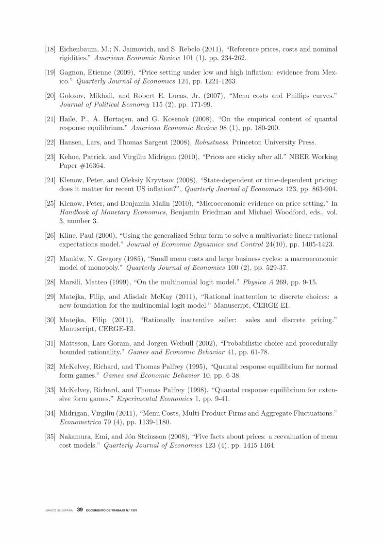
BANCO DE ESPAÑA 39 DOCUMENTO DE TRABAJO N.º 1301
[31] Mattsson, Lars-Goram, and Jorgen Weibull (2002), “Probabilistic choice and procedurallybounded rationality.” Games and Economic Behavior 41, pp. 61-78.
[32] McKelvey, Richard, and Thomas Palfrey (1995), “Quantal response equilibrium for normalform games.” Games and Economic Behavior 10, pp. 6-38.
[33] McKelvey, Richard, and Thomas Palfrey (1998), “Quantal response equilibrium for exten-sive form games.” Experimental Economics 1, pp. 9-41.
[34] Midrigan, Virgiliu (2011), “Menu Costs, Multi-Product Firms and Aggregate Fluctuations.”Econometrica 79 (4), pp. 1139-1180.
[35] Nakamura, Emi, and Jon Steinsson (2008), “Five facts about prices: a reevaluation of menucost models.” Quarterly Journal of Economics 123 (4), pp. 1415-1464.
[18] Eichenbaum, M.; N. Jaimovich, and S. Rebelo (2011), “Reference prices, costs and nominalrigidities.” American Economic Review 101 (1), pp. 234-262.
[19] Gagnon, Etienne (2009), “Price setting under low and high inflation: evidence from Mex-ico.” Quarterly Journal of Economics 124, pp. 1221-1263.
[20] Golosov, Mikhail, and Robert E. Lucas, Jr. (2007), “Menu costs and Phillips curves.”Journal of Political Economy 115 (2), pp. 171-99.
[21] Haile, P., A. Hortacsu, and G. Kosenok (2008), “On the empirical content of quantalresponse equilibrium.” American Economic Review 98 (1), pp. 180-200.
[22] Hansen, Lars, and Thomas Sargent (2008), Robustness. Princeton University Press.
[23] Kehoe, Patrick, and Virgiliu Midrigan (2010), “Prices are sticky after all.” NBER WorkingPaper #16364.
[24] Klenow, Peter, and Oleksiy Kryvtsov (2008), “State-dependent or time-dependent pricing:does it matter for recent US inflation?”, Quarterly Journal of Economics 123, pp. 863-904.
[25] Klenow, Peter, and Benjamin Malin (2010), “Microeconomic evidence on price setting.” InHandbook of Monetary Economics, Benjamin Friedman and Michael Woodford, eds., vol.3, number 3.
[26] Kline, Paul (2000), “Using the generalized Schur form to solve a multivariate linear rationalexpectations model.” Journal of Economic Dynamics and Control 24(10), pp. 1405-1423.
[27] Mankiw, N. Gregory (1985), “Small menu costs and large business cycles: a macroeconomicmodel of monopoly.” Quarterly Journal of Economics 100 (2), pp. 529-37.
[28] Marsili, Matteo (1999), “On the multinomial logit model.” Physica A 269, pp. 9-15.
[29] Matejka, Filip, and Alisdair McKay (2011), “Rational inattention to discrete choices: anew foundation for the multinomial logit model.” Manuscript, CERGE-EI.
[30] Matejka, Filip (2011), “Rationally inattentive seller: sales and discrete pricing.”Manuscript, CERGE-EI.

BANCO DE ESPAÑA 40 DOCUMENTO DE TRABAJO N.º 1301
[36] Reiter, Michael (2009), “Solving heterogeneous-agent models by projection and perturba-tion.” Journal of Economic Dynamics and Control 33 (3), pp. 649-65.
[37] Shannon, Claude (1948), “A mathematical theory of communication.”
[38] Sims, Christopher (2003), “Implications of rational inattention.” Journal of Monetary Eco-nomics 50, pp. 665-90.
[39] Stahl, Dale (1990), “Entropy control costs and entropic equilibrium. ” International Journalof Game Theory 19, pp. 129-138.
[40] Van Damme, Eric (1991), Stability and Perfection of Nash Equilibrium, 2nd edition.Springer Verlag.
[41] Woodford, Michael (2008), “Inattention as a source of randomized discrete adjustment.”Manuscript, Columbia University.
[42] Woodford, Michael (2009), “Information-constrained state-dependent pricing.” Journal ofMonetary Economics 56, pp. S100-S124.
[43] Yun, Tack (2005), “Optimal Monetary Policy with Relative Price Distortions.” AmericanEconomic Review 95 (1), pp. 89-109.
[44] Zbaracki, Mark; Mark Ritson; Daniel Levy; Shantanu Dutta; and Mark Bergen (2004),“Managerial and customer costs of price adjustment: direct evidence from industrial mar-kets.” Review of Economics and Statistics 86 (2), pp. 514-33.

BANCO DE ESPAÑA 41 DOCUMENTO DE TRABAJO N.º 1301
Table 1: Adjustment parameters.
Woodford Woodford PPS PPS Nested Nestedlogit control logit control logit control
λ 0.044 0.045 – – 0.083 0.22
κπ – – 0.049 0.0044 0.013 0.018
κλ 0.0051 0.0080 – – 0.013 0.018
Table 2: Model-Simulated Statistics and Evidence (1% annual inflation)Woodford Woodford PPS PPS Nested Nested Data
logit control logit control logit control
Adjustment frequencyFreq. of price changes 10.2 10.2 10.2 10.2 10.2 10.2 10.2
Price change statisticsMean absolute price change 4.88 4.68 14.0 6.72 8.11 7.51 9.90Std of price changes 5.51 5.27 17.0 7.32 10.1 9.30 13.2Kurtosis of price changes 2.24 2.22 2.58 2.37 3.48 3.40 4.81Percent of price increases 62.7 63.3 55.2 62.3 58.3 58.8 65.1Percent of changes ≤ 5% 47.9 49.7 16.5 27.9 31.5 33.6 35.4
Variability of prices and costsStd(ln p)/Std(ln a) 95.2 91.0 113 97.7 109 104 115∗∗
Costs of decisions and errorsPricing costs∗ 0 0 0 0.174 0 0.509Timing costs∗ 0 0.167 0 0 0 0.361Loss relative to full rationality∗ 0.258 0.416 0.665 0.365 0.582 1.41
Note: All statistics refer to regular consumer price changes excluding sales, and are stated in percent.
Quantities with an asterisk are stated as a percentage of monthly average revenues.
Dataset: Dominick’s, except for double asterisk, which indicates Eichenbaum, Jaimovich and Rebelo (2011).

BANCO DE ESPAÑA 42 DOCUMENTO DE TRABAJO N.º 1301
Table 3: Model-Simulated Statistics and Evidence (63% annual inflation)Woodford Woodford PPS PPS Nested Nested Data
logit control logit control logit control
Freq. of price changes 29.0 29.6 32.1 35.5 24.2 26.0
Mean absolute price change 14.0 13.7 19.7 11.5 17.9 16.6Std of price changes 4.87 4.86 20.1 5.26 11.7 10.9Kurtosis of price changes 3.14 3.12 3.32 6.38 4.64 4.43Percent of price increases 99.9 99.9 78.5 98.9 93.3 93.1Percent of changes ≤ 5% 4.4 4.5 11.2 7.71 7.83 8.71Pricing costs∗ 0 0 0 0.557 0 1.06Timing costs∗ 0 1.00 0 0 0 0.66Loss relative to full rationality∗ 0.752 1.65 1.92 1.00 1.72 3.25
Note: All statistics refer to regular consumer price changes excluding sales, and are stated in percent.
Quantities with an asterisk are stated as a percentage of monthly average revenues.
Dataset: Gagnon (2008) Mexican data.
Table 4: Variance decomposition and Phillips curvesCorrelated money growth shock Woodford Woodford PPS PPS Nested Nested Data∗
(φz = 0.8) logit control logit control logit control
Freq. of price changes (%) 10.2 10.2 10.2 10.2 10.2 10.2 10.2Std of money shock (%) 0.16 0.15 0.16 0.12 0.17 0.17
Std of qtrly inflation (%) 0.25 0.25 0.25 0.25 0.25 0.25 0.25% explained by μ shock alone 100 100 100 100 100 100
Std of qtrly output growth (%) 0.41 0.37 0.34 0.20 0.45 0.43 0.51% explained by μ shock alone 80 73 67 38 89 84
Slope coeff. of Phillips curve* 0.32 0.29 0.31 0.15 0.38 0.35R2 of regression 0.96 0.94 0.999 0.85 0.99 0.98
*The “slope coefficients” are 2SLS estimates of the effect of inflation on consumption
First stage: πqt = α1 + α2μ
qt + εt; second stage: cqt = β1 + β2π
qt + εt, where the instrument
μqt is the exogenous growth rate of the money supply and the superscript q indicates quarterly averages.
Dataset: Dominick’s.

BANCO DE ESPAÑA 43 DOCUMENTO DE TRABAJO N.º 1301
−0.2−0.1
00.1
0.2
−0.20
0.2
0.05
0.1
0.15
0.2
0.25
0.3
cost
Logit probabilities
price5
1015
2025
1020
30
0.2
0.4
0.6
0.8
1
cost
Probability of adjustment
price
cost
pric
e
Density of firms (end of period)
−0.2 −0.15 −0.1 −0.05 0 0.05 0.1 0.15 0.2−0.3
−0.2
−0.1
0
0.1
0.2
cost
pric
e
Density of adjusting firms
−0.2 −0.15 −0.1 −0.05 0 0.05 0.1 0.15 0.2−0.3
−0.2
−0.1
0
0.1
0.2
Notes:
First panel: price distribution conditional on cost.
Second panel: adjustment probability conditional on price and cost.
Third panel: contour plot of density of firms at time of production.
Fourth panel: contour plot of density of adjusting firms.
Figure 1: Price change distributions and adjustment function: nested control cost model.
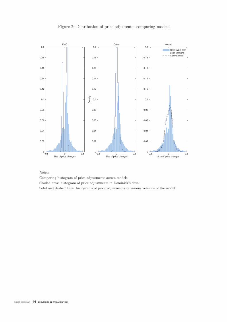
BANCO DE ESPAÑA 44 DOCUMENTO DE TRABAJO N.º 1301
Figure 2: Distribution of price adjustents: comparing models.
−0.5 0 0.50
0.02
0.04
0.06
0.08
0.1
0.12
0.14
0.16
0.18
0.2
Size of price changes
Den
sity
Calvo
−0.5 0 0.50
0.02
0.04
0.06
0.08
0.1
0.12
0.14
0.16
0.18
0.2
Size of price changes
FMC
−0.5 0 0.50
0.02
0.04
0.06
0.08
0.1
0.12
0.14
0.16
0.18
0.2
Size of price changes
Nested
Dominick’s dataLogit versionsControl costs
Notes:
Comparing histogram of price adjustments across models.
Shaded area: histogram of price adjustments in Dominick’s data.
Solid and dashed lines: histograms of price adjustments in various versions of the model.
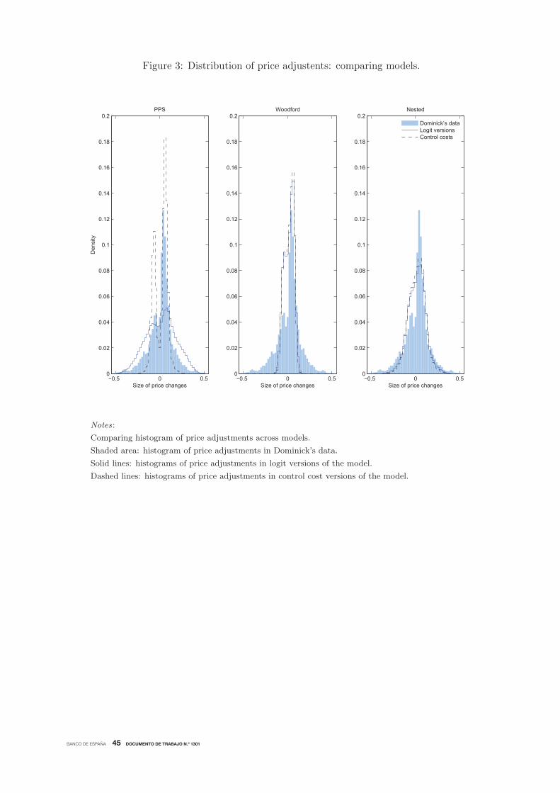
BANCO DE ESPAÑA 45 DOCUMENTO DE TRABAJO N.º 1301
Figure 3: Distribution of price adjustents: comparing models.
−0.5 0 0.50
0.02
0.04
0.06
0.08
0.1
0.12
0.14
0.16
0.18
0.2
Size of price changes
Den
sity
PPS
−0.5 0 0.50
0.02
0.04
0.06
0.08
0.1
0.12
0.14
0.16
0.18
0.2
Size of price changes
Woodford
−0.5 0 0.50
0.02
0.04
0.06
0.08
0.1
0.12
0.14
0.16
0.18
0.2
Size of price changes
Nested
Dominick’s dataLogit versionsControl costs
Notes:
Comparing histogram of price adjustments across models.
Shaded area: histogram of price adjustments in Dominick’s data.
Solid lines: histograms of price adjustments in logit versions of the model.
Dashed lines: histograms of price adjustments in control cost versions of the model.

BANCO DE ESPAÑA 46 DOCUMENTO DE TRABAJO N.º 1301
Figure 4: Losses from failure to adjust: nested control cost model.
−8 −6 −4 −2 0 2 4 6 8 100
0.05
0.1
0.15
0.2
0.25
0.3
0.35
0.4
0.45
0.5Size distribution of losses
Loss as % of average revenue
Den
sity
PotentialRealized
Notes:
Loss from not adjusting, expressed as a percentage of monthly average revenues. Potential losses before adjust-
ments occur (shaded blue) and realized losses after adjustments (black line).
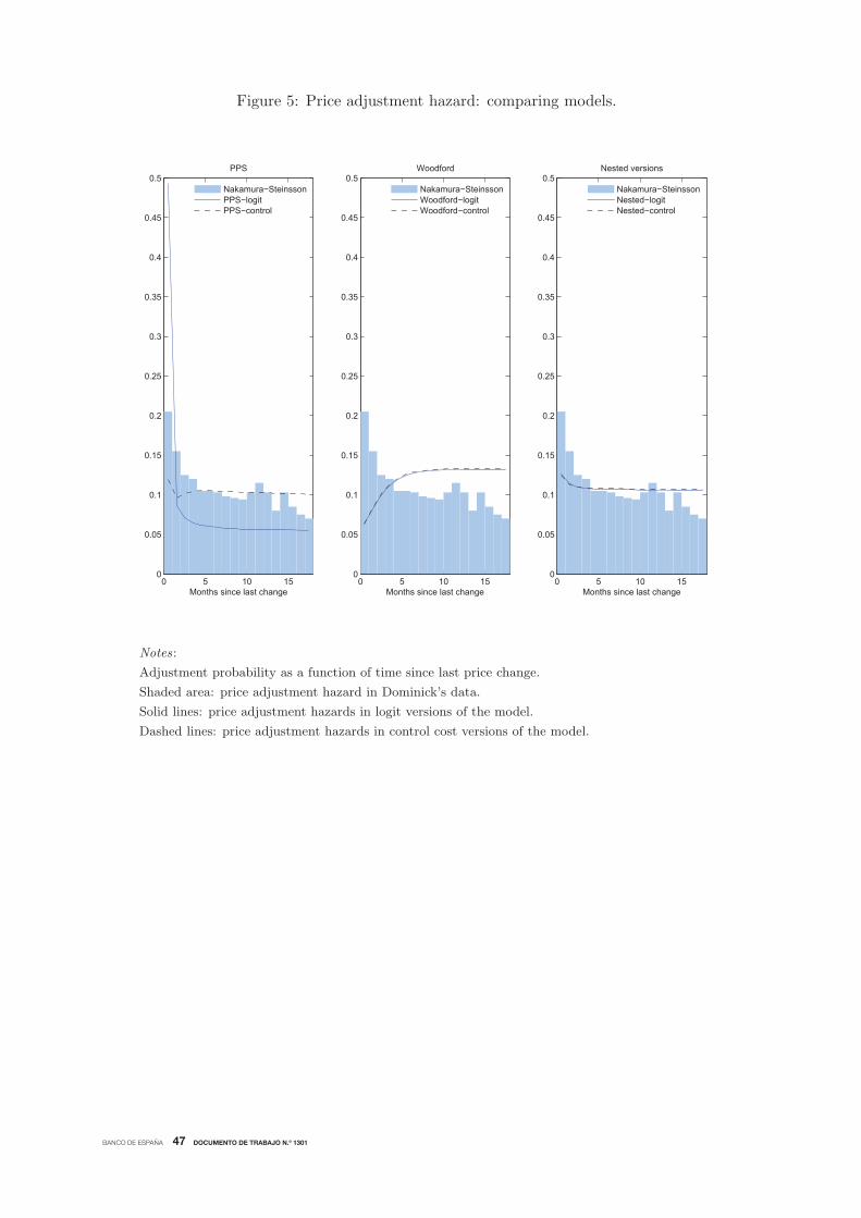
BANCO DE ESPAÑA 47 DOCUMENTO DE TRABAJO N.º 1301
Figure 5: Price adjustment hazard: comparing models.
0 5 10 150
0.05
0.1
0.15
0.2
0.25
0.3
0.35
0.4
0.45
0.5
Months since last change
PPS
Nakamura−SteinssonPPS−logitPPS−control
0 5 10 150
0.05
0.1
0.15
0.2
0.25
0.3
0.35
0.4
0.45
0.5
Months since last change
Woodford
Nakamura−SteinssonWoodford−logitWoodford−control
0 5 10 150
0.05
0.1
0.15
0.2
0.25
0.3
0.35
0.4
0.45
0.5
Months since last change
Nested versions
Nakamura−SteinssonNested−logitNested−control
Notes:
Adjustment probability as a function of time since last price change.
Shaded area: price adjustment hazard in Dominick’s data.
Solid lines: price adjustment hazards in logit versions of the model.
Dashed lines: price adjustment hazards in control cost versions of the model.

BANCO DE ESPAÑA 48 DOCUMENTO DE TRABAJO N.º 1301
Figure 6: Mean adjustment and price duration: comparing models.
0 2 4 6 8 10 120
20
40
60
80
100
120
140
Months since last change
PPS
Klenow−KryvtsovPPS−logitPPS−control
0 2 4 6 8 10 120
20
40
60
80
100
120
140
Months since last change
Siz
e of
pric
e ch
ange
s
Woodford
Klenow−KryvtsovWoodford−logitWoodford−control
0 2 4 6 8 10 120
20
40
60
80
100
120
140
Months since last change
Siz
e of
pric
e ch
ange
s
Nested versions
Klenow−KryvtsovNested−logitNested−control
Notes:
Mean absolute size of price adjustment as function of time since last price change.
Shaded area: Klenow-Kryvstov dataset.
Solid lines: logit versions of the model.
Dashed lines: control cost versions of the model.

BANCO DE ESPAÑA 49 DOCUMENTO DE TRABAJO N.º 1301
Figure 7: Extreme prices tend to be young: comparing models.
−0.2 −0.1 0 0.1 0.20
0.1
0.2
0.3
0.4
0.5
0.6
0.7
0.8
0.9
1
Deviation from average price
Frac
tion
of y
oung
pric
es
PPS
Campbell−EdenPPS−logitPPS−control
−0.2 −0.1 0 0.1 0.20
0.1
0.2
0.3
0.4
0.5
0.6
0.7
0.8
0.9
1
Deviation from average price
Woodford
Campbell−EdenWoodford−logitWoodford−control
−0.2 −0.1 0 0.1 0.20
0.1
0.2
0.3
0.4
0.5
0.6
0.7
0.8
0.9
1
Deviation from average price
Nested
Campbell−EdenNested−logitNested−control
Shaded area: Campbell-Eden dataset.
Solid lines: logit versions of the model.
Dashed lines: control cost versions of the model.
Notes:
Fraction of prices set within the last two months, as a function of deviation from average price
in product class.
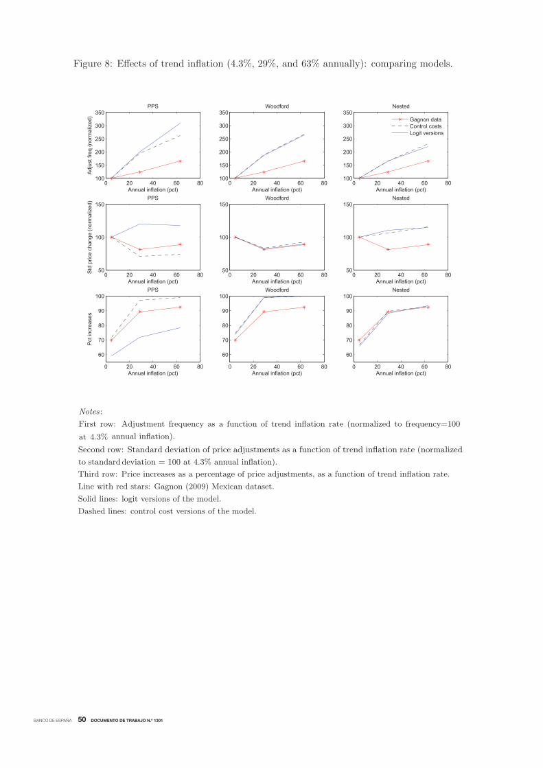
BANCO DE ESPAÑA 50 DOCUMENTO DE TRABAJO N.º 1301
Figure 8: Effects of trend inflation (4.3%, 29%, and 63% annually): comparing models.
0 20 40 60 80100
150
200
250
300
350PPS
Annual inflation (pct)
Adj
ust f
req
(nor
mal
ized
)
0 20 40 60 80100
150
200
250
300
350Woodford
Annual inflation (pct)0 20 40 60 80
100
150
200
250
300
350Nested
Annual inflation (pct)
Gagnon dataControl costsLogit versions
0 20 40 60 8050
100
150PPS
Annual inflation (pct)
Std
pric
e ch
ange
(nor
mal
ized
)
0 20 40 60 8050
100
150Woodford
Annual inflation (pct)0 20 40 60 80
50
100
150Nested
Annual inflation (pct)
0 20 40 60 80
60
70
80
90
100PPS
Annual inflation (pct)
Pct
incr
ease
s
0 20 40 60 80
60
70
80
90
100Woodford
Annual inflation (pct)0 20 40 60 80
60
70
80
90
100Nested
Annual inflation (pct)
Notes:
First row: Adjustment frequency as a function of trend inflation rate (normalized to frequency=100
Second row: Standard deviation of price adjustments as a function of trend inflation rate (normalized
annual inflation).at 4.3%
deviation = 100 at 4.3% annual inflation).to standard )
Third row: Price increases as a percentage of price adjustments, as a function of trend inflation rate.
Line with red stars: Gagnon (2009) Mexican dataset.
Solid lines: logit versions of the model.
Dashed lines: control cost versions of the model.

BANCO DE ESPAÑA 51 DOCUMENTO DE TRABAJO N.º 1301
Figure 9: Impulse responses to money growth shock: comparing models.
0 5 10 15 200
0.5
1
1.5
2
2.5
3
3.5Money growth process
Months0 5 10 15 20
0
0.5
1
1.5
2
2.5
3
3.5Inflation
Months0 5 10 15 20
0
0.5
1
1.5
2
2.5
3
3.5Consumption
Months
FMCCalvoNested−control
Notes:
Impulse responses of inflation and consumption to money growth shock with autocorrelation 0.8 (monthly).
Top row: logit specifications. Bottom row: control cost specifications.
Green lines with squares: Calvo model. Blue lines with circles: FMC model. Red lines: Nested control costs.

BANCO DE ESPAÑA 52 DOCUMENTO DE TRABAJO N.º 1301
Figure 10: Impulse responses to money growth shock: comparing models.
0 5 10 15 200
0.5
1
1.5
2
2.5
3
3.5Money growth process
Months0 5 10 15 20
0
0.5
1
1.5
2
2.5
3
3.5Inflation
Months0 5 10 15 20
0
0.5
1
1.5
2
2.5
3
3.5Consumption
Months
PPS−logitWoodford−logitNested−logit
0 5 10 15 200
0.5
1
1.5
2
2.5
3
3.5Money growth process
Months0 5 10 15 20
0
0.5
1
1.5
2
2.5
3
3.5Inflation
Months0 5 10 15 20
0
0.5
1
1.5
2
2.5
3
3.5Consumption
Months
PPS−controlWoodford−controlNested−control
Notes:
Impulse responses of inflation and consumption to money growth shock with autocorrelation 0.8 (monthly).
Top row: logit specifications. Bottom row: control cost specifications.
Blue lines with circles: PPS versions. Green lines with squares: Woodford versions. Red lines: Nested versions.

BANCO DE ESPAÑA 53 DOCUMENTO DE TRABAJO N.º 1301
Figure 11: Decomposition of inflation impulse responses: comparing models.
0 10 200
0.5
1
1.5
2
2.5
3Intensive margin
Months0 10 20
0
0.5
1
1.5
2
2.5
3Extensive margin
Months0 10 20
0
0.5
1
1.5
2
2.5
3Selection effect
Months0 10 20
0
0.5
1
1.5
2
2.5
3Error margin
Months
PPS-logitWoodford-logitNested-logit
0 10 200
0.5
1
1.5
2
2.5
3Intensive margin
Months0 10 20
0
0.5
1
1.5
2
2.5
3Extensive margin
Months0 10 20
0
0.5
1
1.5
2
2.5
3Selection effect
Months0 10 20
0
0.5
1
1.5
2
2.5
3Error margin
Months
PPS-controlWoodford-controlNested-control
Notes:
Decomposition of inflation impulse response to money growth shock with autocorrelation 0.8 (monthly).
Top row: logit specifications. Bottom row: control cost specifications.
Blue lines with circles: PPS versions. Green lines with squares: Woodford versions. Red lines: Nested versions.
BANCO DE ESPAÑA PUBLICATIONS
WORKING PAPERS
1201 CARLOS PÉREZ MONTES: Regulatory bias in the price structure of local telephone services.
1202 MAXIMO CAMACHO, GABRIEL PEREZ-QUIROS and PILAR PONCELA: Extracting non-linear signals from several
economic indicators.
1203 MARCOS DAL BIANCO, MAXIMO CAMACHO and GABRIEL PEREZ-QUIROS: Short-run forecasting of the euro-dollar
exchange rate with economic fundamentals.
1204 ROCIO ALVAREZ, MAXIMO CAMACHO and GABRIEL PEREZ-QUIROS: Finite sample performance of small versus
large scale dynamic factor models.
1205 MAXIMO CAMACHO, GABRIEL PEREZ-QUIROS and PILAR PONCELA: Markov-switching dynamic factor models in
real time.
1206 IGNACIO HERNANDO and ERNESTO VILLANUEVA: The recent slowdown of bank lending in Spain: are supply-side
factors relevant?
1207 JAMES COSTAIN and BEATRIZ DE BLAS: Smoothing shocks and balancing budgets in a currency union.
1208 AITOR LACUESTA, SERGIO PUENTE and ERNESTO VILLANUEVA: The schooling response to a sustained Increase in
low-skill wages: evidence from Spain 1989-2009.
1209 GABOR PULA and DANIEL SANTABÁRBARA: Is China climbing up the quality ladder?
1210 ROBERTO BLANCO and RICARDO GIMENO: Determinants of default ratios in the segment of loans to households in
Spain.
1211 ENRIQUE ALBEROLA, AITOR ERCE and JOSÉ MARÍA SERENA: International reserves and gross capital fl ows.
Dynamics during fi nancial stress.
1212 GIANCARLO CORSETTI, LUCA DEDOLA and FRANCESCA VIANI: The international risk-sharing puzzle is at business-
cycle and lower frequency.
1213 FRANCISCO ALVAREZ-CUADRADO, JOSE MARIA CASADO, JOSE MARIA LABEAGA and DHANOOS
SUTTHIPHISAL: Envy and habits: panel data estimates of interdependent preferences.
1214 JOSE MARIA CASADO: Consumption partial insurance of Spanish households.
1215 J. ANDRÉS, J. E. BOSCÁ and J. FERRI: Household leverage and fi scal multipliers.
1216 JAMES COSTAIN and BEATRIZ DE BLAS: The role of fi scal delegation in a monetary union: a survey of the political
economy issues.
1217 ARTURO MACÍAS and MARIANO MATILLA-GARCÍA: Net energy analysis in a Ramsey-Hotelling growth model.
1218 ALFREDO MARTÍN-OLIVER, SONIA RUANO and VICENTE SALAS-FUMÁS: Effects of equity capital on the interest rate
and the demand for credit. Empirical evidence from Spanish banks.
1219 PALOMA LÓPEZ-GARCÍA, JOSÉ MANUEL MONTERO and ENRIQUE MORAL-BENITO: Business cycles and
investment in intangibles: evidence from Spanish fi rms.
1220 ENRIQUE ALBEROLA, LUIS MOLINA and PEDRO DEL RÍO: Boom-bust cycles, imbalances and discipline in Europe.
1221 CARLOS GONZÁLEZ-AGUADO and ENRIQUE MORAL-BENITO: Determinants of corporate default: a BMA approach.
1222 GALO NUÑO and CARLOS THOMAS: Bank leverage cycles.
1223 YUNUS AKSOY and HENRIQUE S. BASSO: Liquidity, term spreads and monetary policy.
1224 FRANCISCO DE CASTRO and DANIEL GARROTE: The effects of fi scal shocks on the exchange rate in the EMU and
differences with the US.
1225 STÉPHANE BONHOMME and LAURA HOSPIDO: The cycle of earnings inequality: evidence from Spanish social
security data.
1226 CARMEN BROTO: The effectiveness of forex interventions in four Latin American countries.
1227 LORENZO RICCI and DAVID VEREDAS: TailCoR.
1228 YVES DOMINICY, SIEGFRIED HÖRMANN, HIROAKI OGATA and DAVID VEREDAS: Marginal quantiles for stationary
processes.
1229 MATTEO BARIGOZZI, ROXANA HALBLEIB and DAVID VEREDAS: Which model to match?
1230 MATTEO LUCIANI and DAVID VEREDAS: A model for vast panels of volatilities.
1231 AITOR ERCE: Does the IMF’s offi cial support affect sovereign bond maturities?
1232 JAVIER MENCÍA and ENRIQUE SENTANA: Valuation of VIX derivatives.

1233 ROSSANA MEROLA and JAVIER J. PÉREZ: Fiscal forecast errors: governments vs independent agencies?
1234 MIGUEL GARCÍA-POSADA and JUAN S. MORA-SANGUINETTI: Why do Spanish fi rms rarely use the bankruptcy
system? The role of the mortgage institution.
1235 MAXIMO CAMACHO, YULIYA LOVCHA and GABRIEL PEREZ-QUIROS: Can we use seasonally adjusted indicators
in dynamic factor models?
1236 JENS HAGENDORFF, MARÍA J. NIETO and LARRY D. WALL: The safety and soundness effects of bank M&As in the EU:
Does prudential regulation have any impact?
1237 SOFÍA GALÁN and SERGIO PUENTE: Minimum wages: do they really hurt young people?
1238 CRISTIANO CANTORE, FILIPPO FERRONI and MIGUEL A. LEÓN-LEDESMA: The dynamics of hours worked and
technology.
1239 ALFREDO MARTÍN-OLIVER, SONIA RUANO and VICENTE SALAS-FUMÁS: Why did high productivity growth of banks
precede the fi nancial crisis?
1240 MARIA DOLORES GADEA RIVAS and GABRIEL PEREZ-QUIROS: The failure to predict the Great Recession. The failure
of academic economics? A view focusing on the role of credit.
1241 MATTEO CICCARELLI, EVA ORTEGA and MARIA TERESA VALDERRAMA: Heterogeneity and cross-country spillovers in
macroeconomic-fi nancial linkages.
1242 GIANCARLO CORSETTI, LUCA DEDOLA and FRANCESCA VIANI: Traded and nontraded goods prices, and
international risk sharing: an empirical investigation.
1243 ENRIQUE MORAL-BENITO: Growth empirics in panel data under model uncertainty and weak exogeneity.
1301 JAMES COSTAIN and ANTON NAKOV: Logit price dynamics.
Unidad de Servicios AuxiliaresAlcalá, 48 - 28014 Madrid
Telephone +34 91 338 6368 E-mail: [email protected]
www.bde.es