Demand Forecasting of Individual Probability DensityFunctions with Machine Learning

Felix Wick1, Ulrich Kerzel3, Martin Hahn1, Moritz Wolf1, Trapti Singhal2, DanielStemmer1, Jakob Ernst1, and Michael Feindt1

1Blue Yonder GmbH (Ohiostraße 8, 76149 Karlsruhe, Germany)

2Blue Yonder India Private Limited (Bengaluru, India)3IU Internationale Hochschule (Erfurt, Germany)

Demand forecasting is a central component of the replen-ishment process for retailers, as it provides crucial inputfor subsequent decision making like ordering processes. Incontrast to point estimates, such as the conditional meanof the underlying probability distribution, or confidence in-tervals, forecasting complete probability density functionsallows to investigate the impact on operational metrics,which are important to define the business strategy, overthe full range of the expected demand. Whereas metricsevaluating point estimates are widely used, methods forassessing the accuracy of predicted distributions are rare,and this work proposes new techniques for both qualitativeand quantitative evaluation methods. Using the supervisedmachine learning method “Cyclic Boosting”, complete in-dividual probability density functions can be predictedsuch that each prediction is fully explainable. This isof particular importance for practitioners, as it allows toavoid “black-box” models and understand the contributingfactors for each individual prediction. Another crucialaspect in terms of both explainability and generalizabilityof demand forecasting methods is the limitation of theinfluence of temporal confounding, which is prevalent inmost state of the art approaches.

Keywords: explainable machine learning, retaildemand forecasting, probability distribution, tem-poral confounding

DOI: 10.1007/s43069-021-00079-8

Published in Springer Nature Operations Research Fo-rum.

1. Introduction

One of the main business operations of retailers is to ensurethat sufficient goods are available in the store for customersto buy. This entails two parts: In a first step, we needto estimate the future customer demand to be able tojudge how many goods we will need to order from thesupplier or wholesaler, given the current inventory level.In the second step, aimed at inventory control, we needto place the actual orders, which is further complicatedby the fact that multiple operational constraints, such

as lot-sizes or delivery schedules, need to be includedin the final ordering decision. Unfortunately, from theperspective of the retailer, the two parts, estimating thefuture demand and optimization of the order quantity, donot factorize into two separate issues, but are inextricablylinked. This is because the business strategy depends onthe complete chain of demand estimation and subsequentreplenishment process to control the inventory. We canunderstand this in the following way: In the simplestcase, a retailer might want to optimize their profit, orequivalently the cost, by reducing the impact of perishableitems that have not been sold at the end of the sellingperiod, as well as the lost revenue by not being able tomeet the customer demand within this period. This isknown as the “newsvendor problem” [1], see, e.g., [2] for adetailed review. Assuming linear overage (h) and underage(b) cost, the optimal quantile qopt = b/(b+ h) of a knownprobability density function (PDF) describing demand asrandom variable can be calculated exactly. This quantilethen corresponds to the numerical value of the demandPDF prediction that can be used to determine the optimalorder quantity.

In reality, the situation is often more complex, as manyfactors may contribute to the cost function. Further-more, the cost function may vary between individual stock-keeping units (SKU) and may also change with time. How-ever, the general principle remains: If we have access tothe relevant cost function, we can determine the optimalpoint estimator of the future demand from the associatedPDF, see Appendix A. For the case of a relatively sim-ple cost function, such as the mean squared error (MSE)or the mean absolute deviation (MAD), the calculationsare straight-forward. If the cost function becomes morecomplex, we may no longer be able to perform the calcu-lations analytically, but will have to resort to numericalapproaches. Furthermore, if we can predict more than onequantile, we can investigate the effect of choosing differentquantiles, and determine, for example, how sensitive opera-tional metrics, such as stockout or waste rate of perishablegoods, change. This can be done using, for example, abusiness-oriented simulation that starts from the quantilesof the predicted demand for each SKU to simulate the

1

arX

iv:2

009.

0705

2v3

[cs

.LG

] 2

2 Ju

l 202

1

value of the business-relevant KPIs for each setting, takingoperational constraints into account. This can then beused, for example, to align the business strategy. Predict-ing the full demand PDF therefore allows the maximumflexibility for further optimizations, because we have directaccess to all quantiles.

Due to its stochastic nature, demand is difficult to fore-cast: It depends on many influencing factors and, as al-ready stated above, we can interpret it as a random variablewith associated probability distribution. And as such, de-mand is neither identically and independently distributed(i.i.d.) between different products and sales locations, norbetween different times. This means that, while we cangenerally assume that demand follows a specific type ofPDF, its parameters are unique to the instance for whichan estimate is required. For example, the PDF describingthe demand of a particular product-location-date combina-tion is specific to the product, date, and retail location forwhich the forecast is made. Furthermore, this distributiondepends on a wide range of influencing factors, such asseasonal effects, sales price, local weather, etc. Therefore,in order to predict the expected demand for each SKUat each sales location and sales day, we need to forecastindividual probability distributions rather than globallyadjusted parameters for groups of SKUs, locations, or salesdays.

If we account for the cases where demand exceeds thecurrent stock level, resulting in out-of-stock situations,the actual demand in the past can be approximated byrealized sales. We can then understand the time-orderedobservations of sales events as a time series of a randomvariable. It is therefore tempting to use established timeseries regression models to predict the future values ofthe expected demand. However, if we wish to use thepredicted values for anything but the prediction itself, wehave to be careful to avoid, or at least limit as much aspossible, temporal confounding, which emerges if someexternal variable X causally influences several time stepst of the observed time series variable Y , say Yt and Yt−lag,where “lag” denotes a specific time difference between thetwo steps. In the case of a retailer, Yt is the demand fora specific product at a given sales location for a specificday, and X can be, for example, the price of the product,which we can set as part of our business strategy or changeaccording to some promotion. This dependency creates abackdoor path between Yt−lag and Yt, that in turn leadsto a spurious autocorrelation between the values of Y atdifferent times t, if we cannot control for the confounderX. This is particularly important for the case of demandforecasting, since customer demand is not a natural phe-nomenon we observe as an outsider, but retailers activelyinfluence the customer demand through a wide range of in-terventions, such as a given assortment choice, promotions,advertisements, coupons, etc. If we cannot disentanglethe fundamental causal dependencies from the spuriousautocorrelation, understanding the influences that lead toa specific prediction becomes very challenging, even if theunderlying prediction method itself is fully explainable.Moreover, due to this disguising of actual causal dependen-cies, reliance on temporal confounding is also detrimentalin terms of generalizability of the forecasting model. The

issue of temporal confounding, together with a proposedsolution, is discussed in more detail in sec. 5.

Demand forecasting for retailers often requires to pre-dict millions of product-location combinations each day.Univariate time series forecasting methods operate on eachof these many individual time series separately. On theother hand, supervised machine learning (ML) algorithmsoptimize all individual time series simultaneously, whichcan enhance the generalizability of the method by exploit-ing common aspects between the various time series. Thiscan lead to a drastic reduction in variance of the model,and in turn to an improvement of the forecast quality ofeach of the individual time series. Furthermore, machinelearning provides a straight-forward way to include themany exogenous variables that influence demand as fea-tures (or covariates) of the model. This can also help toimprove the forecast quality compared to methods mainlyrelying on autocorrelation of the historic sales.

Hence, in order for a retailer to be able to use demandforecasts most effectively, we need to be able to:

• Predict the future demands on SKU level at requiredtemporal granularity as complete individual PDFs.

• Avoid temporal confounding in the model used forthe prediction of the future demand.

• Evaluate that each part of the PDF models the ob-served data appropriately.

• Ideally, each prediction is fully explainable, enablingoperational experts to exactly understand what con-tributed to it.

The remainder of the paper is organized as follows: Wefirst review the relevant literature and existing work insec. 2. We then describe our method to predict individualnegative binomial PDFs using a parametric approach in-cluding two distinct machine learning models for mean andvariance in sec. 3. After that, we describe novel techniquesfor the qualitative and quantitative evaluation of PDF pre-dictions in sec. 4. This is followed by a detailed discussionon temporal confounding in sec. 5. And finally, we presenta demand forecasting example to show an application ofour methods in sec. 6.

Summary of Contributions

This work brings together elements from three differentfields: operations research, machine learning, and causalinference. The combination of these allows to build state-of-the-art demand forecasting models that are fully ex-plainable and incorporate the causal structure of demand.The contribution of this paper is twofold:

Using the explainable machine learning algorithm CyclicBoosting [3], we show how complete probability distribu-tions of the future demand of individual products in retailstores can be predicted at the operationally required gran-ularity. In particular, we show how using machine learning,the detrimental effects of temporal confounding, that areintrinsic to many methods used for time series forecasting,can be limited. The impact of temporal confounding inthe context of time series forecasting has not been widely

2

investigated so far in the scientific literature, and to thebest of our knowledge this is the first discussion withinthe context of demand forecasting.

Furthermore, we show how predictions of full individualprobability distributions, no matter if created by an ap-proach with or without assumption of a specific distributionclass, can be evaluated qualitatively and quantitatively,such that we can assess whether both overall functionalform (in the case of a parametric approach) as well asspecific quantiles are predicted correctly. This allows toverify that the predicted demand distribution appropri-ately reflects the observed data in terms of model choiceand forecast accuracy.

The general methods developed in this paper can beapplied to any setting that requires the prediction andevaluation of probability distributions from observationaldata, not just demand forecasting. However, to make theimpact and benefits more tangible in a practical setting,as well as describe a general methodology how to buildsuch systems from a practitioner’s perspective, we limitthe discussion to demand forecasting in retail.

2. Literature Review

Demand forecasting is one of the core operational activi-ties of any customer-facing business and accurate demandpredictions are vital to the optimization of the businessoperations. This is of particular concern, for example,for supermarkets, as their profit margin tend to be verylow, e.g., 1% and lower for European discounters [4] toabout 4% for regular supermarkets [5, 6] to about 8% inthe USA [7]. It can be approached in a variety of ways,see, e.g., [8] for a survey of methods used in retail salesforecasting with a particular focus on fashion retail.

A popular approach is to treat the demand as a timeseries, i.e., as a time-ordered sequence of observed salesevents. In this setting, the future demand can be predictedas a point estimate using auto-regressive integrated movingaverage (ARIMA) [9] or exponential smoothing [10–13] ap-proaches. See also [14] for a comprehensive overview overtraditional time series forecasting methods. Essentially,these methods extrapolate the future values by buildingsome form of regression model based on past observa-tions, i.e., yt+1 = f(yt, yt−1, . . .), introducing dedicatedfunctional components for trends, seasonality, or externalfactors in various ways, depending on the exact modelingapproach taken. The main underlying concept behindthese approaches is to exploit the autocorrelation betweenvalues of the variable Y at different times t. Intuitively,we assume that the sequence of events observed so faris a good predictor of future events. Examples for thesemethods in the context of demand forecasting can be foundin, e.g., [15–18]. A different approach is to use a conceptfrom engineering, the Kalman filter [19], and apply it tostatistical forecasting [20]. Examples for this method usedto estimate demand are, e.g., [21–24]. Starting from theconcept of Kalman filters, state space models [25] relatethe measured values over time to the evolution of (un-known) states of the considered system. A comparisonof the performance of ARIMA and state space models

in a retail setting can be found, e.g., in [26]. Structuraltime series models [27] take a similar approach and decom-pose the observations into components for trend, seasonal-ity, and others. A modern implementation is Facebook’s“Prophet” [28]. Several other approaches are known in theliterature as well: Kok and Fisher [29] model the demandbased on the average demand for a product, modified by alogistic regression for the number of customers in a store,purchase incidence, and product choice. Wang et al. [30]model the demand under the assumption of a Poissonprocess.

Alternatively to the methods discussed above, time seriesforecasts in general and demand predictions in particu-lar can be approached by means of supervised machinelearning methods, using the values of the time series to bepredicted as target, i.e., the numbers the machine learningalgorithm is trained to predict. For example, see [31,32] forapplications of neural networks for time series forecasting.Machine learning approaches can include multiple covari-ates. This allows to include not only past sales data, butalso information about prices, promotions, or details aboutthe article or store in the forecast. There are two main ap-proaches for time series forecasting using machine learning:We either assume that the variables are independent ran-dom variables (for both prediction target and potentiallytime-dependent features) for each time step of the differ-ent time series, or we consider the full sequences of timesteps as a whole, resulting in a single sample (includingprediction target and potentially time-dependent features)for each individual time series. For the case of individualsamples for different time steps, in order to combine theendogenous information from the target autocorrelationwith all other exogenous features, the most prominent ap-proach is to include lagged target information explicitly viastacking of univariate time series predictions for the targetas features in the machine learning model. For example,we could add exponentially smoothed moving averageswith a range of damping factors as features into the model.An example for the estimation of future demand in thecontext of price optimization, using regression trees [33],can be found in [34]. For the case of sequence samples,deep learning methods such as recurrent neural networks(RNN) [35], especially in form of “long short-term memory”(LSTM) networks [36], or transformers [37], based on theself-attention mechanism, are used. These methods employinformation about the prediction target autocorrelationimplicitly via the input sequences of the time-ordered train-ing events. Both concepts, LSTM cells and self-attention,aim at learning the elements of the individual time seriesfrom the data that are deemed important for the predic-tion of the future values by the algorithm. The interestin deep learning approaches for demand forecasting hasincreased significantly recently, see, e.g., [38–42]. A reviewof deep learning methods for time series forecasting in awide range of applications can also be found in [43], andthe use of RNNs with focus on industrial applications isdiscussed in [44]. A further approach is to explore the useof generative adversarial networks [45] in the context oftime series forecasting [46–48].

In many situations, relying on the exploitation of auto-correlation, either via traditional time series forecasting or

3

machine learning approaches, is sufficient. However, thiscan lead to shortcomings in terms of explainability and gen-eralizability due to temporal confounding. There are twomain paths to avoid this: One way is to explicitly accountfor the confounders and extend the model to include them.The main challenge is then the discovery of temporal con-founders and, for example, try to learn the causal structurefrom the observational data, see, e.g., [49–51]. This topicis of particular importance in fields like medicine [52] orclimate research [53]. Brodersen et al. [54, 55] propose touse Bayesian structural time series models to estimate thecausal effect of interventions on a time series by creatinga counterfactual prediction that describes the behavior ofthe time series had the intervention not taken place. Whilestructural time series equations allow to model componentssuch as trend, seasonality, and others explicitly, the fun-damental form of the state equation is Yt = GtYt−1 + εt,where εt ∼ N (0, σ2) is a white noise term and Gt somematrix that describes the evolution from the state Yt−1 toYt. Therefore, great care must be taken to avoid temporalconfounding when setting up the states for structural timeseries models. Compared to fields like medicine, market-ing, and many others that focus on the causal impact offew or just one intervention(s), retailers have to includemany external effects that affect the predicted demand andare repeated frequently: Prices are changed dynamically,advertisements placed, new products are included in theassortment and others removed, etc.The alternative to the above approaches is to separate theautocorrelation from exogenous information via a chain ofindependent models (see sec. 5).

Common to all approaches discussed so far is that theypredict a point estimate, essentially a single number thatindicates the next value in the sequence, for example, thenumber of a specific product likely to be sold in a givenstore on a particular opening day. While operational deci-sions can be based on such a single number, this does notallow us to evaluate the uncertainty on such a prediction.Since the model parameters are not a priori known butestimated from data, the predicted values are generallyassociated with an uncertainty that needs to be quantified.Several methods have been developed, and Chatfield [56]reviews the methods available at the time. In particular,bootstrapping methods for auto-regressive time series fore-casting have been proposed, see, e.g., [57–66]. However, asalready pointed out in [56], estimating the uncertainty ofthe point forecast is only one reason to go beyond a pointestimate. For example, if we want to be able to evaluatestrategies for a range of different outcomes, we need accessto more information. In particular, if we do not wish tomake the assumption that the point forecast is the meanof an underlying Gaussian distribution, that can be fullyspecified by the point forecast and an interval, we needto be able to compute any quantile of the distribution orestimate the full PDF directly.

Generally, quantile regression [67] can be implementedin various frameworks and used to estimate a range ofquantiles for each predicted distribution, from which anempirical probability distribution can be interpolated. Us-ing a dedicated neural network [68], either the full PDF ora defined range of quantiles can be calculated directly from

the data for each individual prediction without assuming anunderlying model. Focusing on time series, Hyndman [69]proposes to use either a simulation or bootstrapping frame-work to estimate the highest density forecast regions ofnon-normal time series. Tay [70] summarizes the use ofdensity forecasts in applications in finance and economics.Using RNNs, quantile regression for multiple forecastinghorizons [71] has been used to predict the demand at theinternet retailer Amazon. Using an attention-based ar-chitecture, the Temporal Fusion Transformer (TFT) [72]can also predict a set of specified quantiles at each pre-dicted time step. Another possibility to model the un-derlying data distribution without assumption of a fixeddistribution class is the usage of conditional normalizingflows [73, 74], which aim to transform a simple initial den-sity into a more complex one by applying a sequence ofinvertible transformations.

Alternatively, we can start from a model assumptionfor the demand distribution and fit the model parametersinstead of reconstructing the complete distribution [75,76].This approach is computationally favorable and usuallymore robust, as fewer parameters need to be estimated.Empirically, we can determine the best fitting distributionfrom data [77]. However, given the stochastic nature ofdemand, such an empirically determined distribution isnot expected to be stable and prone to sudden changes.Instead, the choice of the demand distribution should bemotivated by theoretic considerations. Discrete demandis typically modeled as a negative binomial distribution(NBD), also known as Gamma-Poisson distribution [78–82]. This distribution arises if the Poisson parameterµ is a random variable itself, which follows a Gammadistribution. The NBD has two parameters, the mean µand the variance σ2 > µ, and is over-dispersed compared tothe Poisson distribution, for which σ2 = µ. Hence, for eachordering decision, the model parameters µ and σ2 needto be determined at the required granularity, typically foreach item, sales location, and ordering time, depending onall auxiliary data describing article details, retail location,and influencing factors such as pricing and advertisementinformation.

Finally, since from an operational perspective the re-tailer’s focus is less on the demand prediction per se but onthe decisions, in particular, the ordering decisions, that arederived from these, we need to consider the question if weshould skip the separate step of estimating the demand anddirectly predict the optimal order quantity. This directapproach is often referred to as “data-driven newsven-dor” in the recent literature, see, e.g., [83–87]. It aimsto avoid estimating the underlying PDF for demand anduse the available data (historic sales records and furthervariables) to derive the operational decisions (i.e., the or-der quantity) directly. Although the integrated approachseems preferable at first glance, since it avoids determin-ing the full demand distribution and results directly inthe desired operational decision, the indirect approachvia demand forecasts offers some substantial advantages.First, demand forecasts in form of full PDFs can be usedto simulate the performance of the relevant metrics onthe level of individual items, and, for example, optimizethe impact on business strategy decisions on conflicting

4

metrics such as out-of-stock (i.e., lost sales) and waste rate.From a practitioners perspective, separating the demandforecast from the operational decisions (i.e., calculatingthe order quantities for the next delivery cycle) enableslonger-term planning and reduces the complexity, as itavoids coupling delivery schedules of multiple wholesalersand manufacturers with the forecast of customer demand.It also allows to share long-term demand predictions withother business units or external vendors and wholesalersto ease their planning for the production and supply chainprocesses upstream of the retailer. From the perspective ofthe industrial practice of a vendor of supply chain methodsand tools, modeling the demand separately from derivingthe subsequent orders has the additional benefit that mul-tiple retail chains can benefit from any improvement inthe model description, even if the specific retailers are un-related to each other. Additionally, a purely data-drivenapproach going from the observed data directly to theoperational decision (such as the order quantity) doesnot allow to analyze the data-generating process, i.e., themechanism behind the stochastic behavior of the customerdemand. This is crucial, for example, if a causal analysisis planned, such as a study of the effect of promotions,advertisements, price changes, or other demand shapingfactors in either Pearl’s do-calculus [88] or Rubin’s poten-tial outcomes framework [89]. We should note that this isdifferent compared to Granger causality [90], that seeks todetermine the causal influence one time series has on an-other. In our case, price changes, promotions, and similarare interventions that we actively pursue in order to influ-ence demand. In Pearl’s do-calculus, we can express this,for example, as P (demand |do(Price=2.99Euro)). Whilewe can, of course, represent the prices as a chronologicallyordered series of numbers, it is not really a time series buta sequence of interventions. Using an operational quantity,such as the order quantity, will in most cases act as aninsufficient proxy for the quantity of interest (customerdemand) and likely lead to unnecessary causal pathwaysthat we may not be able to fully control for.

3. Negative Binomial PDF Estimation

To predict an individual PDF using a parametric approach,one has to rely on a model assumption about the underlyingdistribution of the random variable to be predicted. Asdiscussed earlier, the NBD is well routed in theoreticalarguments to model customer demand. Its parameters canbe modeled by two independent models, one to estimatethe mean and the other for the variance. At least inprinciple, any method can be used. However, as discussedin sec. 2, machine learning algorithms are ideally suitedfor the task of demand forecasting and in the following,we will use the Cyclic Boosting algorithm to benefit inparticular from explainable decisions rather than black-box approaches. Furthermore, the regularization approachused during the training of the Cyclic Boosting algorithmallows a dedicated treatment of the underlying NBD model,which is another major benefit compared to a standard“off-the-shelf” machine learning algorithm. This meanswe use two subsequent Cyclic Boosting models in order

to estimate the parameters of each individual PDF thatwe need to forecast. The first model is used to estimatethe mean and the second to estimate the variance. Thefeatures may or may not differ between the mean andvariance estimation models, and it can be beneficial toinclude the corresponding mean predictions as feature inthe variance model. The assigned mean and variancepredictions can then be used to generate individual PDFsusing the parameterization of the NBD for each sample.

In the following, after a brief recap of the fundamentalideas of Cyclic Boosting, we describe a method to predictmean and variance for individual NBDs using two CyclicBoosting models.

3.1. Cyclic Boosting Algorithm: Mean estimation

Cyclic Boosting [3] is a type of generalized additive modelusing a cyclic coordinate descent optimization and featur-ing a boosting-like update of parameters. Major benefitsof Cyclic Boosting are its accuracy, performance, even atlarge scale, and providing fully explainable predictions,which are of vital importance in practical applications.

The main idea of this algorithm is the following: First,each feature, denoted by index j, is discretized appropri-ately into k bins to reflect the specific behavior of thefeature. The global mean c is determined from all valuesy of the target variable Y ∈ [0,∞) observed in the data.Single data records, for example, the sales correspondingto a specific product-location-date combination (meaningthe sales record of a specific item sold on a specific day ata specific sales location) along with all relevant features,are indexed by i. The individual predictions for the NBDmean, denoted by µi, can then be calculated as:

µi = c ·p∏j=1

fkj with k = {xj,i ∈ bkj } (1)

The factors fkj are the model parameters that are deter-mined iteratively from the features until the algorithmconverges. During training, regularization techniques areapplied to avoid overfitting and improve the generalizationability of the algorithm. The deviation of each factor fromfkj = 1 can then be used to explain how a specific featurecontributes to each individual prediction.

In detail, the following meta-algorithm describes howthe model parameters fkj are obtained from the trainingdata:

1. Calculate the global average c from all observed yacross all bins k and features j.

2. Initialize the factors fkj ← 1

3. Cyclically iterate through features j = 1, ..., p andcalculate in turn for each bin k the partial factors gand corresponding aggregated factors f , where indicest (current iteration) and τ (current or preceding iter-ation) refer to iterations of full feature cycles as thetraining of the algorithm progresses:

gkj,t =

∑xj,i∈bkj

yi∑xj,i∈bkj

µi,τwhere fkj,t =

t∏s=1

gkj,s (2)

5

Here, g is a factor that is multiplied to the correspond-ing ft−1 in each iteration. The current prediction, µτ ,is calculated according to Eqn. (1) with the currentvalues of the aggregated factors f :

µi,τ = c ·p∏j=1

fkj,τ (3)

To be precise, the determination of gkj,t for a specific

feature j uses fkj,t−1 in the calculation of µ. For thefactors of all other features, the newest available valuesare used, i.e., depending on the sequence of featuresin the algorithm, either from the current (τ = t) orthe preceding iteration (τ = t− 1).

4. Quit when stopping criteria, e.g., the maximum num-ber of iterations or no further improvement of an errormetric such as the MAD or MSE, are met at the endof a full feature cycle.

3.2. Cyclic Boosting Algorithm: Width estimation

In the previous section, the general Cyclic Boosting algo-rithm was used to estimate the mean of the NBD model.In order to predict the variance of the NBD model (as-sociated with the mean predicted before), we modify thealgorithm as follows: When looking at the demand of in-dividual product-location-date combinations, the targetvariable y has the values y = 0, 1, 2, ... and the NBD modelcan be parameterized as in [91]:

NBD(y;µ, r) =Γ(r + y)

y! · Γ(r)·(

r

r + µ

)r·(

µ

r + µ

)y, (4)

where µ is the mean of the distribution and r a dispersionparameter.

By bounding the inverse of the dispersion parameter 1/rto the interval [0, 1] (corresponding to bounding r to theinterval [1,∞]), the variance σ2 can be calculated from µand r via:

σ2 = µ+µ2

r(5)

The estimate of the dispersion parameter r can thenbe calculated by minimizing the loss function defined inEqn. (6), which is expressed as negative log-likelihoodfunction of an NBD. The minimization over all input sam-ples i is performed with respect to the Cyclic Boostingparameters fkj , constituting the model of ri, according toEqn. (7), where the estimates for the mean µi are fixed tothe values obtained from the mean model described in sec.3.1.

L(r) = −L(r) = − ln∑i

NBD(yi; µi, ri) (6)

ri = 1 +1

p∏j=1

fkj

with k = {xj,i ∈ bkj } (7)

In other words, the values ri are estimated via learningthe Cyclic Boosting model parameters fkj for each featurej and bin k from data. For any concrete observation i,

the index k of the bin is determined by the value of thefeature xj,i and the subsequent look-up into which bin thisobservation falls. Like in sec. 3.1, the model parametersfkj correspond to factors with values in [0,∞], and again

values deviating from fkj = 1 can be used to explain therelative importance of a specific feature contributing toindividual predictions. Note that the structure of Eqn. (7)can be interpreted as inverse of a logit link function in thesame way as explained in [3] when Cyclic Boosting is usedfor classification tasks.

In the same way as described in sec. 3.1 for its basicmultiplicative regression mode, the Cyclic Boosting algo-rithm is trained iteratively using cyclic coordinate descent,processing one feature with all its bins at a time untilconvergence is reached. However, unlike in Eqn. (2) of thebasic multiplicative regression mode, the minimization ofthe loss function in Eqn. (6) cannot be solved analyticallyand has to be done numerically, for example, using a ran-dom search. All other advantages of Cyclic Boosting, likeindividual explainability of predictions, remain valid forits negative binomial width mode.

Finally, the variance σ2i can be estimated from the dis-

persion parameter ri using Eqn. (5). And together with theindividual predicted mean µi from the first step, the NBDmodel is then fully specified for each individual predictioni.

4. Evaluation of PDF Predictions

Many statistical and most machine learning methods donot provide a full PDF as result. Instead, these methodstypically predict a single numerical quantity (usually de-noted by y, in this work denoted by µ to make evidentthat it is the prediction of the mean of an underlying prob-ability distribution) that is then compared to the observedconcrete realization of the random variable (denoted byy) using metrics such as the MSE, MAD, or others. Inthe setting of a retailer, the observed quantity is the salesof individual products and most approaches would thenpredict a single number as a direct estimate of the sales.However, reducing the prediction to a single number doesnot allow to account for the uncertainty of the predictionor the dynamics of the system. Instead, it is imperative topredict the full PDF for each prediction to be able to opti-mize the subsequent operational decision. Unfortunately,most statistical or machine learning methods that predictfull individual probability functions lack quantitative oreven qualitative evaluation methods to assess whether thefull distribution has been forecasted correctly, in particularin its tails.

In the simplest case, we only have one model with oneset of model parameters to cover all predictions. In thiscase, the evaluation of the full PDF is straightforward: Wewould fill a histogram of all observed values, such as salesrecords, and overlay this with the single model, such asan NBD with predicted parameters, that is used for allobservations. Then, we compare the model curve directlywith the observations, using statistical tests such as theKolmogorov-Smirnov test.

In practical applications however, we have a large num-

6

ber of effective prediction models, since although we mayalways use the same model parameterization, such as theNBD, its parameters have to be determined at the requiredlevel of granularity. For example, for daily orders, we needto predict the parameters of the NBD for each product,location, and sales day. Unlike the simple case discussedabove, where we had many observations to compare theprediction model to, we now have just a single observationper prediction, meaning that we cannot use statistical testsdirectly.

For an estimation of the determining parameters of anassumed functional form for the PDF, assessing the correct-ness of the PDF model output refers to the evaluation ofthe accuracy of the prediction of the different parameters.In the case of the NBD used in this work, we have to verifythat mean and variance are determined accurately, as wellas checking that the choice of the underlying model candescribe the observed data.

In the following, we will show how different visualizationsof the observed cumulative distribution function (CDF)values can be used to evaluate the quality of the predictedPDFs. Although we limit the following discussion to thenegative binomial model, the method can be applied gener-ally to any representation of a PDF, even if it is obtainedempirically.

4.1. Histogram of CDF Observations

For a first qualitative assessment, we make use of theprobability integral transform, see, e.g., [63, 92], whichstates that a random variable distributed according to theCDF of another random variable is uniformly distributedbetween 0 and 1. We therefore expect that the distributionof the actually observed CDF values of the correspondingindividual PDF predictions is uniform, if the predictedPDF is calibrated correctly, regardless of the shape of thepredicted distribution. Any deviation can be interpretedas a hint that the predicted PDF is not fully correct [93].The CDF of a PDF f(x) is defined as:

FX(x) = P (X ≤ x) =

∫ x

−∞fX(x′)dx′ (8)

Here, FX(x) is the CDF with limx→−∞ FX(x) = 0 andlimx→∞ Fx(x) = 1. The cumulative distribution describesthe probability that the variable has a value smaller thanx, and intuitively represents the area under f(x′) up to apoint x.

If the CDF is continuous and strictly increasing, thenthe inverse of the CDF, F−1(y), exists and is a uniquereal-valued number x for each y ∈ [0, 1], so that we canwrite F (x) = y. The inverse of the CDF is also called thequantile function, because we can define the quantile q ofthe PDF f(x) as:

Qq = F−1(q) (9)

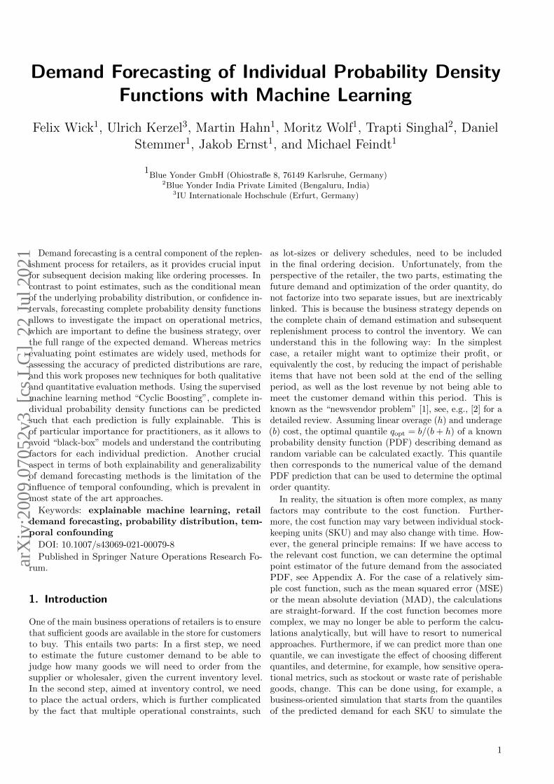
Using the example of the normal distribution withN (0, 1) as shown in Fig. 1, we can identify the median(q = 0.5) by first looking at the CDF in the lower part ofthe figure, look at the value 0.5 on the y axis and thenidentify the point on the x axis for both the PDF f(x)

0.0

0.1

0.2

0.3

0.4f(x)

4 3 2 1 0 1 2 3 40.0

0.2

0.4

0.6

0.8

1.0F(x)

Figure 1: PDF f(x) and CDF F (x) of a normal distribu-tion.

and the CDF F (x) that corresponds to the quantile q. Inthe case of the normal distribution, this is of course thecentral value at zero.

We can then interpret the CDF as a new variable s =F (t), meaning that F becomes a transformation that mapst to s, i.e., F : t→ s. Accordingly, limt→−∞ s(t) = 0 andlimt→∞ s(t) = 1, and s can be intuitively interpreted asthe fraction of the distribution of t with values smallerthan t from the definition of the CDF. This implies thatthe PDF of s, g(s), is constant in the interval s ∈ [0, 1] inwhich s is defined, and s can be interpreted as the CDFof its own PDF:

s = G(s) =

∫ s

−∞g(s′)ds′ (10)

In case of discrete probability distributions, such as theNBD, the same argument still holds, but the definition ofthe quantile function is replaced by the generalized inverse:F−1(y) = inf {x : F(x) > y} for y ∈ [0, 1], see e.g., [92,p. 54]. In order to obtain a uniform distribution fordiscrete PDFs that is comparable to the case of continuousdistributions, the histogram holding the values of the CDFis filled using random numbers according to the intervalsof the CDF. For example, if the sales of zero items accountfor 75 percent of the observed sales distribution for thisitem, the value of the CDF function that is used to fill thehistogram in case of zero actual sales is randomly chosenin the interval [0, 0.75]. Proceeding similarly for all otherobserved values, with the intervals from which to randomlychoose values to fill in the histogram defined by the CDFvalues of the corresponding discrete sales value and theone below (e.g., for 3 actual sales: random pick betweendiscrete CDF values for 2 and 3), the resulting histogram ofCDF values is again uniform, as in the case of a continuousPDF.

A histogram of the actually observed CDF values foreach individual PDF prediction (see Fig. 7 for an example)is therefore expected to be uniformly distributed in [0, 1],if the predicted PDF f(x) is correctly calibrated, i.e., ifboth the choice of the model and the model parameters areestimated correctly. If the mean or the variance are not

7

0.0 0.2 0.4 0.6 0.8 1.0CDF values

0

1000

2000

3000

4000

5000

6000

coun

t

a)

broad

0.0 0.2 0.4 0.6 0.8 1.0CDF values

0

1000

2000

3000

4000

5000

6000

coun

t

b)

narrow

0.0 0.2 0.4 0.6 0.8 1.0CDF values

0

1000

2000

3000

4000

5000

6000

coun

t

c)

over

0.0 0.2 0.4 0.6 0.8 1.0CDF values

0

1000

2000

3000

4000

5000

6000

coun

t

d)

under

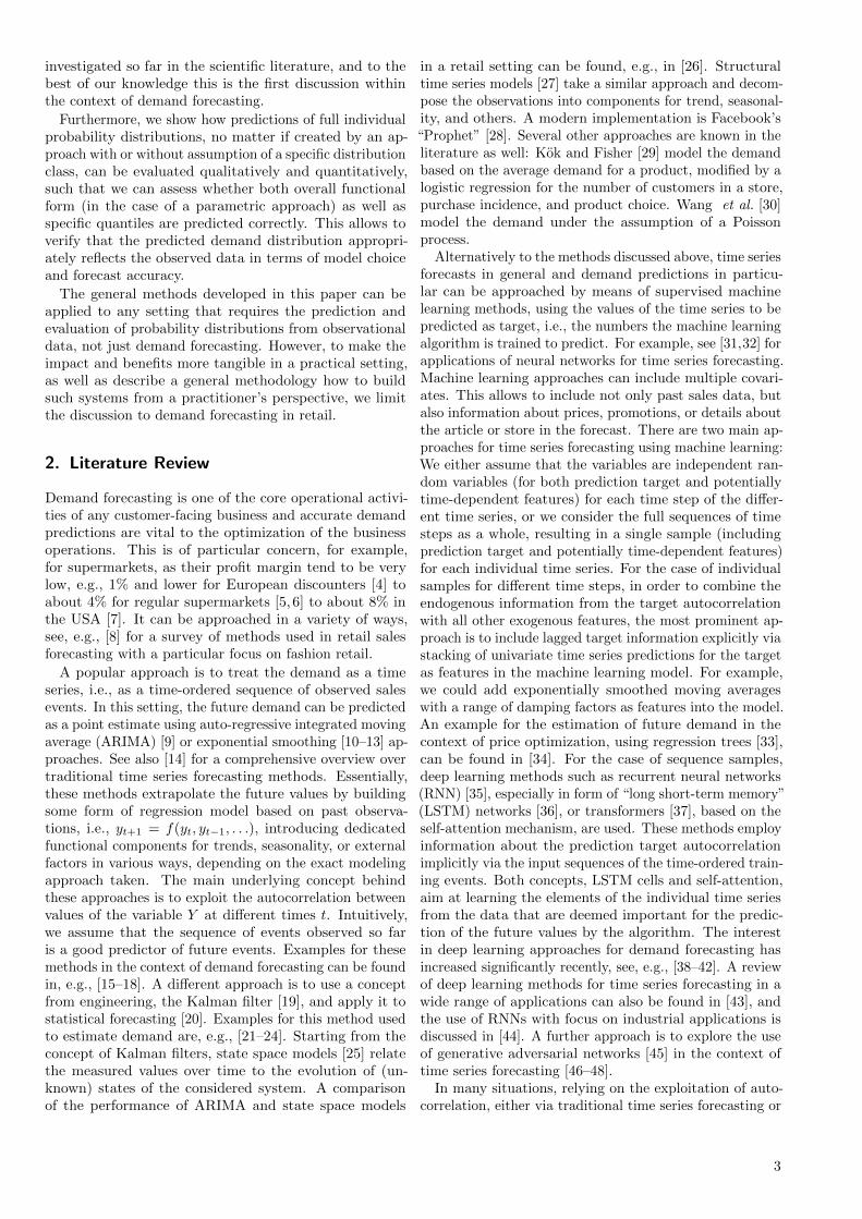
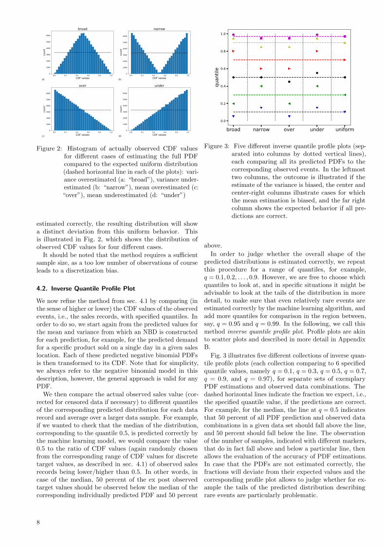
Figure 2: Histogram of actually observed CDF valuesfor different cases of estimating the full PDFcompared to the expected uniform distribution(dashed horizontal line in each of the plots): vari-ance overestimated (a: “broad”), variance under-estimated (b: “narrow”), mean overestimated (c:“over”), mean underestimated (d: “under”)

estimated correctly, the resulting distribution will showa distinct deviation from this uniform behavior. Thisis illustrated in Fig. 2, which shows the distribution ofobserved CDF values for four different cases.

It should be noted that the method requires a sufficientsample size, as a too low number of observations of courseleads to a discretization bias.

4.2. Inverse Quantile Profile Plot

We now refine the method from sec. 4.1 by comparing (inthe sense of higher or lower) the CDF values of the observedevents, i.e., the sales records, with specified quantiles. Inorder to do so, we start again from the predicted values forthe mean and variance from which an NBD is constructedfor each prediction, for example, for the predicted demandfor a specific product sold on a single day in a given saleslocation. Each of these predicted negative binomial PDFsis then transformed to its CDF. Note that for simplicity,we always refer to the negative binomial model in thisdescription, however, the general approach is valid for anyPDF.

We then compare the actual observed sales value (cor-rected for censored data if necessary) to different quantilesof the corresponding predicted distribution for each datarecord and average over a larger data sample. For example,if we wanted to check that the median of the distribution,corresponding to the quantile 0.5, is predicted correctly bythe machine learning model, we would compare the value0.5 to the ratio of CDF values (again randomly chosenfrom the corresponding range of CDF values for discretetarget values, as described in sec. 4.1) of observed salesrecords being lower/higher than 0.5. In other words, incase of the median, 50 percent of the ex post observedtarget values should be observed below the median of thecorresponding individually predicted PDF and 50 percent

broad narrow over under uniform0.0

0.2

0.4

0.6

0.8

1.0

quan

tile

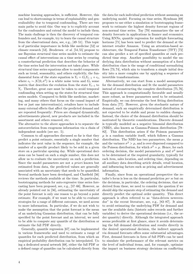
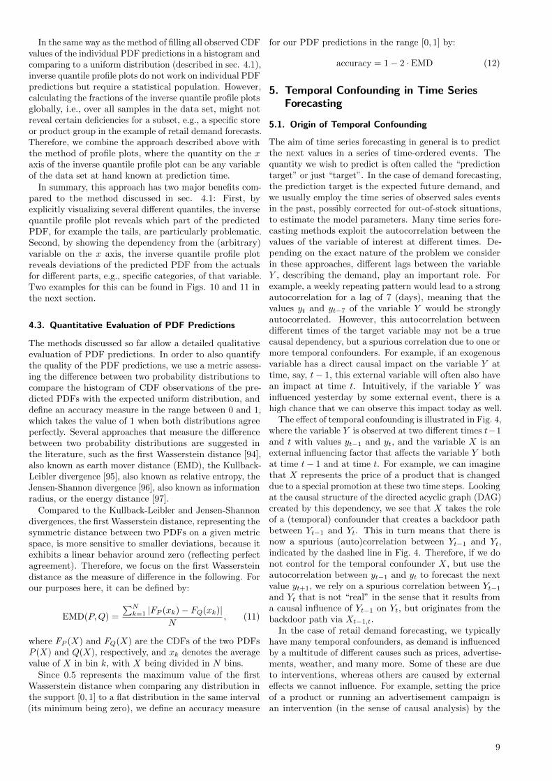
Figure 3: Five different inverse quantile profile plots (sep-arated into columns by dotted vertical lines),each comparing all its predicted PDFs to thecorresponding observed events. In the leftmosttwo columns, the outcome is illustrated if theestimate of the variance is biased, the center andcenter-right columns illustrate cases for whichthe mean estimation is biased, and the far rightcolumn shows the expected behavior if all pre-dictions are correct.

above.

In order to judge whether the overall shape of thepredicted distributions is estimated correctly, we repeatthis procedure for a range of quantiles, for example,q = 0.1, 0.2, . . . , 0.9. However, we are free to choose whichquantiles to look at, and in specific situations it might beadvisable to look at the tails of the distribution in moredetail, to make sure that even relatively rare events areestimated correctly by the machine learning algorithm, andadd more quantiles for comparison in the region between,say, q = 0.95 and q = 0.99. In the following, we call thismethod inverse quantile profile plot. Profile plots are akinto scatter plots and described in more detail in AppendixB.

Fig. 3 illustrates five different collections of inverse quan-tile profile plots (each collection comparing to 6 specifiedquantile values, namely q = 0.1, q = 0.3, q = 0.5, q = 0.7,q = 0.9, and q = 0.97), for separate sets of exemplaryPDF estimations and observed data combinations. Thedashed horizontal lines indicate the fraction we expect, i.e.,the specified quantile value, if the predictions are correct.For example, for the median, the line at q = 0.5 indicatesthat 50 percent of all PDF prediction and observed datacombinations in a given data set should fall above the line,and 50 percent should fall below the line. The observationof the number of samples, indicated with different markers,that do in fact fall above and below a particular line, thenallows the evaluation of the accuracy of PDF estimations.In case that the PDFs are not estimated correctly, thefractions will deviate from their expected values and thecorresponding profile plot allows to judge whether for ex-ample the tails of the predicted distribution describingrare events are particularly problematic.

8

In the same way as the method of filling all observed CDFvalues of the individual PDF predictions in a histogram andcomparing to a uniform distribution (described in sec. 4.1),inverse quantile profile plots do not work on individual PDFpredictions but require a statistical population. However,calculating the fractions of the inverse quantile profile plotsglobally, i.e., over all samples in the data set, might notreveal certain deficiencies for a subset, e.g., a specific storeor product group in the example of retail demand forecasts.Therefore, we combine the approach described above withthe method of profile plots, where the quantity on the xaxis of the inverse quantile profile plot can be any variableof the data set at hand known at prediction time.

In summary, this approach has two major benefits com-pared to the method discussed in sec. 4.1: First, byexplicitly visualizing several different quantiles, the inversequantile profile plot reveals which part of the predictedPDF, for example the tails, are particularly problematic.Second, by showing the dependency from the (arbitrary)variable on the x axis, the inverse quantile profile plotreveals deviations of the predicted PDF from the actualsfor different parts, e.g., specific categories, of that variable.Two examples for this can be found in Figs. 10 and 11 inthe next section.

4.3. Quantitative Evaluation of PDF Predictions

The methods discussed so far allow a detailed qualitativeevaluation of PDF predictions. In order to also quantifythe quality of the PDF predictions, we use a metric assess-ing the difference between two probability distributions tocompare the histogram of CDF observations of the pre-dicted PDFs with the expected uniform distribution, anddefine an accuracy measure in the range between 0 and 1,which takes the value of 1 when both distributions agreeperfectly. Several approaches that measure the differencebetween two probability distributions are suggested inthe literature, such as the first Wasserstein distance [94],also known as earth mover distance (EMD), the Kullback-Leibler divergence [95], also known as relative entropy, theJensen-Shannon divergence [96], also known as informationradius, or the energy distance [97].

Compared to the Kullback-Leibler and Jensen-Shannondivergences, the first Wasserstein distance, representing thesymmetric distance between two PDFs on a given metricspace, is more sensitive to smaller deviations, because itexhibits a linear behavior around zero (reflecting perfectagreement). Therefore, we focus on the first Wassersteindistance as the measure of difference in the following. Forour purposes here, it can be defined by:

EMD(P,Q) =

∑Nk=1 |FP (xk)− FQ(xk)|

N, (11)

where FP (X) and FQ(X) are the CDFs of the two PDFsP (X) and Q(X), respectively, and xk denotes the averagevalue of X in bin k, with X being divided in N bins.

Since 0.5 represents the maximum value of the firstWasserstein distance when comparing any distribution inthe support [0, 1] to a flat distribution in the same interval(its minimum being zero), we define an accuracy measure

for our PDF predictions in the range [0, 1] by:

accuracy = 1− 2 · EMD (12)

5. Temporal Confounding in Time SeriesForecasting

5.1. Origin of Temporal Confounding

The aim of time series forecasting in general is to predictthe next values in a series of time-ordered events. Thequantity we wish to predict is often called the “predictiontarget” or just “target”. In the case of demand forecasting,the prediction target is the expected future demand, andwe usually employ the time series of observed sales eventsin the past, possibly corrected for out-of-stock situations,to estimate the model parameters. Many time series fore-casting methods exploit the autocorrelation between thevalues of the variable of interest at different times. De-pending on the exact nature of the problem we considerin these approaches, different lags between the variableY , describing the demand, play an important role. Forexample, a weekly repeating pattern would lead to a strongautocorrelation for a lag of 7 (days), meaning that thevalues yt and yt−7 of the variable Y would be stronglyautocorrelated. However, this autocorrelation betweendifferent times of the target variable may not be a truecausal dependency, but a spurious correlation due to one ormore temporal confounders. For example, if an exogenousvariable has a direct causal impact on the variable Y attime, say, t− 1, this external variable will often also havean impact at time t. Intuitively, if the variable Y wasinfluenced yesterday by some external event, there is ahigh chance that we can observe this impact today as well.

The effect of temporal confounding is illustrated in Fig. 4,where the variable Y is observed at two different times t−1and t with values yt−1 and yt, and the variable X is anexternal influencing factor that affects the variable Y bothat time t− 1 and at time t. For example, we can imaginethat X represents the price of a product that is changeddue to a special promotion at these two time steps. Lookingat the causal structure of the directed acyclic graph (DAG)created by this dependency, we see that X takes the roleof a (temporal) confounder that creates a backdoor pathbetween Yt−1 and Yt. This in turn means that there isnow a spurious (auto)correlation between Yt−1 and Yt,indicated by the dashed line in Fig. 4. Therefore, if we donot control for the temporal confounder X, but use theautocorrelation between yt−1 and yt to forecast the nextvalue yt+1, we rely on a spurious correlation between Yt−1and Yt that is not “real” in the sense that it results froma causal influence of Yt−1 on Yt, but originates from thebackdoor path via Xt−1,t.

In the case of retail demand forecasting, we typicallyhave many temporal confounders, as demand is influencedby a multitude of different causes such as prices, advertise-ments, weather, and many more. Some of these are dueto interventions, whereas others are caused by externaleffects we cannot influence. For example, setting the priceof a product or running an advertisement campaign isan intervention (in the sense of causal analysis) by the

9

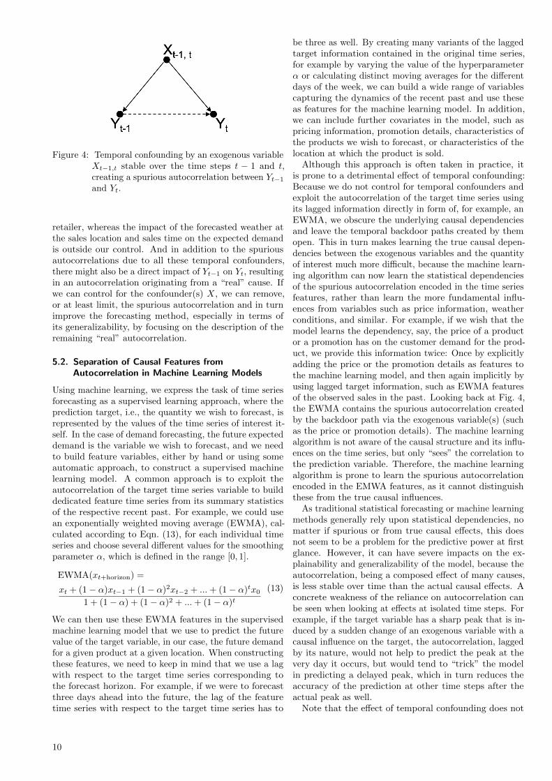
Figure 4: Temporal confounding by an exogenous variableXt−1,t stable over the time steps t − 1 and t,creating a spurious autocorrelation between Yt−1and Yt.

retailer, whereas the impact of the forecasted weather atthe sales location and sales time on the expected demandis outside our control. And in addition to the spuriousautocorrelations due to all these temporal confounders,there might also be a direct impact of Yt−1 on Yt, resultingin an autocorrelation originating from a “real” cause. Ifwe can control for the confounder(s) X, we can remove,or at least limit, the spurious autocorrelation and in turnimprove the forecasting method, especially in terms ofits generalizability, by focusing on the description of theremaining “real” autocorrelation.

5.2. Separation of Causal Features fromAutocorrelation in Machine Learning Models

Using machine learning, we express the task of time seriesforecasting as a supervised learning approach, where theprediction target, i.e., the quantity we wish to forecast, isrepresented by the values of the time series of interest it-self. In the case of demand forecasting, the future expecteddemand is the variable we wish to forecast, and we needto build feature variables, either by hand or using someautomatic approach, to construct a supervised machinelearning model. A common approach is to exploit theautocorrelation of the target time series variable to builddedicated feature time series from its summary statisticsof the respective recent past. For example, we could usean exponentially weighted moving average (EWMA), cal-culated according to Eqn. (13), for each individual timeseries and choose several different values for the smoothingparameter α, which is defined in the range [0, 1].

EWMA(xt+horizon) =

xt + (1− α)xt−1 + (1− α)2xt−2 + ...+ (1− α)tx01 + (1− α) + (1− α)2 + ...+ (1− α)t

(13)

We can then use these EWMA features in the supervisedmachine learning model that we use to predict the futurevalue of the target variable, in our case, the future demandfor a given product at a given location. When constructingthese features, we need to keep in mind that we use a lagwith respect to the target time series corresponding tothe forecast horizon. For example, if we were to forecastthree days ahead into the future, the lag of the featuretime series with respect to the target time series has to

be three as well. By creating many variants of the laggedtarget information contained in the original time series,for example by varying the value of the hyperparameterα or calculating distinct moving averages for the differentdays of the week, we can build a wide range of variablescapturing the dynamics of the recent past and use theseas features for the machine learning model. In addition,we can include further covariates in the model, such aspricing information, promotion details, characteristics ofthe products we wish to forecast, or characteristics of thelocation at which the product is sold.

Although this approach is often taken in practice, itis prone to a detrimental effect of temporal confounding:Because we do not control for temporal confounders andexploit the autocorrelation of the target time series usingits lagged information directly in form of, for example, anEWMA, we obscure the underlying causal dependenciesand leave the temporal backdoor paths created by themopen. This in turn makes learning the true causal depen-dencies between the exogenous variables and the quantityof interest much more difficult, because the machine learn-ing algorithm can now learn the statistical dependenciesof the spurious autocorrelation encoded in the time seriesfeatures, rather than learn the more fundamental influ-ences from variables such as price information, weatherconditions, and similar. For example, if we wish that themodel learns the dependency, say, the price of a productor a promotion has on the customer demand for the prod-uct, we provide this information twice: Once by explicitlyadding the price or the promotion details as features tothe machine learning model, and then again implicitly byusing lagged target information, such as EWMA featuresof the observed sales in the past. Looking back at Fig. 4,the EWMA contains the spurious autocorrelation createdby the backdoor path via the exogenous variable(s) (suchas the price or promotion details). The machine learningalgorithm is not aware of the causal structure and its influ-ences on the time series, but only “sees” the correlation tothe prediction variable. Therefore, the machine learningalgorithm is prone to learn the spurious autocorrelationencoded in the EMWA features, as it cannot distinguishthese from the true causal influences.

As traditional statistical forecasting or machine learningmethods generally rely upon statistical dependencies, nomatter if spurious or from true causal effects, this doesnot seem to be a problem for the predictive power at firstglance. However, it can have severe impacts on the ex-plainability and generalizability of the model, because theautocorrelation, being a composed effect of many causes,is less stable over time than the actual causal effects. Aconcrete weakness of the reliance on autocorrelation canbe seen when looking at effects at isolated time steps. Forexample, if the target variable has a sharp peak that is in-duced by a sudden change of an exogenous variable with acausal influence on the target, the autocorrelation, laggedby its nature, would not help to predict the peak at thevery day it occurs, but would tend to “trick” the modelin predicting a delayed peak, which in turn reduces theaccuracy of the prediction at other time steps after theactual peak as well.

Note that the effect of temporal confounding does not

10

only apply to this specific approach of building featuressuch as the EMWA to be used in supervised machinelearning, but to all time series forecasting methods thatrely on the autocorrelation between events at various lags,including ARIMA, Holt-Winters, Kalman filters and therelated variants, RNNs and its variants like LSTMs, andothers summarized in sec. 2.

In order to avoid these issues, we suggest to separate thetarget autocorrelation from the exogenous dependencies.This can be done by avoiding any features in the machinelearning model that include lagged target information.Using the example from above, this would mean thatwe include features such as the price of the product orpromotion details, weather information, as well as othervariables describing the characteristics of a given productat a specific sales location, but do not include laggedinformation from the sales time series, such as its EWMAor similar approaches.

Therefore, the features do not include any variable thatis directly constructed from the previously observed salesevents. As a consequence, the machine learning modelneeds to learn from the true causal dependencies expressedin the exogenous features, which improves both the explain-ability of the predictions, as well as the generalizability ofthe prediction model, because the causal dependencies arenot confused by additional spurious autocorrelations. Itshould be noted that variables describing certain seasonaleffects, like the day of the week or the day of the year, canbe included in the machine learning model without anynegative effects. In fact, these represent seasonal causaldependencies of the target.

We need to keep in mind that, although this approachof handling temporal confounders improves the predictionmodel used for demand forecasting, it is not yet sufficientfor true causal inferences. For this, we would also have tocontrol for the confounding effects between the differentexogenous features of the machine learning model and itsprediction target.

5.3. Autocorrelated Residual Correction

By including all available exogenous variables as features inthe machine learning model but excluding any endogenousinformation from the target autocorrelation we can, atleast partially, control for the temporal confounders. Anyremaining autocorrelation between different lags of thetime series of the residuals formed from the original timeseries and the time series of the forecasted values fromthe machine learning model discussed above can thereforeoriginate from two reasons: Either there is a genuineautocorrelation between different lags Yt−lag and Yt of thevariable we wish to forecast, or we have not included allrelevant causal variables in the machine learning model.To make use of this remaining autocorrelation, we suggestto apply a residual correction on each of the predictionsof the machine learning model µML (assuming predictionsof the mean of an underlying PDF as discussed in sec. 3),based on the deviations in the recent past between thetarget and these predictions. Such a residual correctionheuristically captures the recent trends without modelingthem explicitly, and can be seen as an empirical correction

to improve the final forecast quality.One possibility for the implementation of the residual

correction is to apply exponential smoothing. In the sim-plest case, this can be done as stated in eqn. 14, wherethe two EWMA terms are grouped by the individual timeseries and calculated according to eqn. 13.

µ =EWMA(y)

EWMA(µML)· µML (14)

In most cases, simple exponential smoothing will be suf-ficient for the residual correction, since we have alreadyincorporated all relevant external effects, including season-alities like a dependency of the target on the day of theweek, in the machine learning model before, and only seekto capture the information that we have missed, because,for example, we do not have the relevant data to describethis as a further feature variable. However, we need to beaware that if we have missed a crucial temporal confounderwhen building the features for the machine learning model,applying this residual correction risks opening a backdoorpath for this confounder, which in turn might result inslightly sub-optimal predictions, as discussed in sec. 5.1.We should therefore take care to use the relevant domainknowledge to capture the causal structure of the prob-lem at hand as best as we can. On the other hand, themethod proposed above does allow us to take temporalconfounders into account at all, and we are only limitedby the extend of our domain knowledge, or to capturethe relevant data, to identify and include the temporalconfounders as exogenous feature variables in the machinelearning model.

6. Example: Retail Demand Forecasting

In the following, we describe how to use the approachoutlined above in a practical setting. We use a publicdataset obtained from a Kaggle online competition focus-ing on estimating unit sales of Walmart retail goods [98]for individual items for specific stores on specific days. Foreach demand forecast, Cyclic Boosting is used to predictthe full probability distribution of the expected demandat a granularity of (item, store, day) and use the methodsdescribed in sec. 4 to evaluate the quality of the indi-vidual forecasts. Each data record corresponding to anobserved sales record is described by the following fields:the identifier of an individual store (store id), the prod-uct identifier (item id), and the date(date). The targety, that we need to predict, is the number of sales of agiven product in a given store on a specific day, denotedby sales.

For our experiments, we use data from 2013-01-01 to2016-05-22, that describe the sales of 100 different products(FOODS 3 500, ..., FOODS 3 599) of the department FOODS 3

in all 10 available stores. All data before 2016 are usedas the training data, and the data from 2016 are usedas an independent test set. Besides the fields used toidentify an individual sales record and the correspondingobserved sales value, namely item id, store id, date,sales, we also use the fields event name 1, event type 1,snap CA, snap TX, snap WI, sell price, and list price,

11

and multiple features built from these variables are thenincluded in the machine learning models.

6.1. Mean Estimation

As discussed earlier, we assume that each individual salecan be described by a Poisson-like process and we assumean NBD to model the individual probability distributionof each sales event. As a first step, we use the supervisedmachine learning method Cyclic Boosting (as described insec. 3.1) to predict the mean of the distribution.

This model uses the following variables as features: cate-gorical variables for store id and item id, several derivedvariables that are constructed from the time series of thesales records describing trend and seasonality (days sincebeginning of 2013 as linear trend as well as day of week,day of year, month, and week of month), time windowsaround the events given in the data set (7 days beforeuntil 3 days after for Christmas and Easter, and 3 daysbefore until 1 day after for all other events like New Year orThanksgiving), a flag denoting a promotion, and the ratioof reduced (sell price) and normal price (list price).We also include various two-dimensional combinations ofthese features. In these cases, one of the two dimensions iseither store id or item id, allowing the machine learningmodel to learn characteristics of individual locations andproducts.As discussed in sec. 5, we do not use any lagged target in-formation, for example via the inclusion of target EWMAfeatures, in the machine learning model, but apply anindividual residual correction on each of its predictions,which accounts for deviations between the EWMA (withα = 0.15) of the predictions and targets of each product-location combination over the corresponding past. Empiri-cally, a value of α = 0.15 gives good results here, thoughin a practical application, this parameter would have to beoptimized using methods such as cross-validation accord-ing to a metric that reflects the objective of the businessstrategy. To reflect a realistic replenishment scenario, weuse the model to predict the expected demand two daysinto the future, meaning that we use a lag of two daysfor the calculation of both the target EWMA and theprediction EWMA.

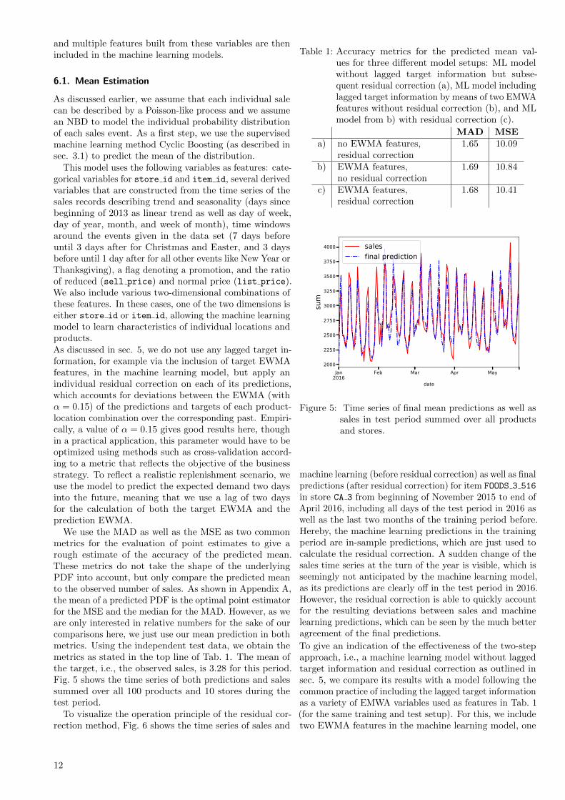
We use the MAD as well as the MSE as two commonmetrics for the evaluation of point estimates to give arough estimate of the accuracy of the predicted mean.These metrics do not take the shape of the underlyingPDF into account, but only compare the predicted meanto the observed number of sales. As shown in Appendix A,the mean of a predicted PDF is the optimal point estimatorfor the MSE and the median for the MAD. However, as weare only interested in relative numbers for the sake of ourcomparisons here, we just use our mean prediction in bothmetrics. Using the independent test data, we obtain themetrics as stated in the top line of Tab. 1. The mean ofthe target, i.e., the observed sales, is 3.28 for this period.Fig. 5 shows the time series of both predictions and salessummed over all 100 products and 10 stores during thetest period.

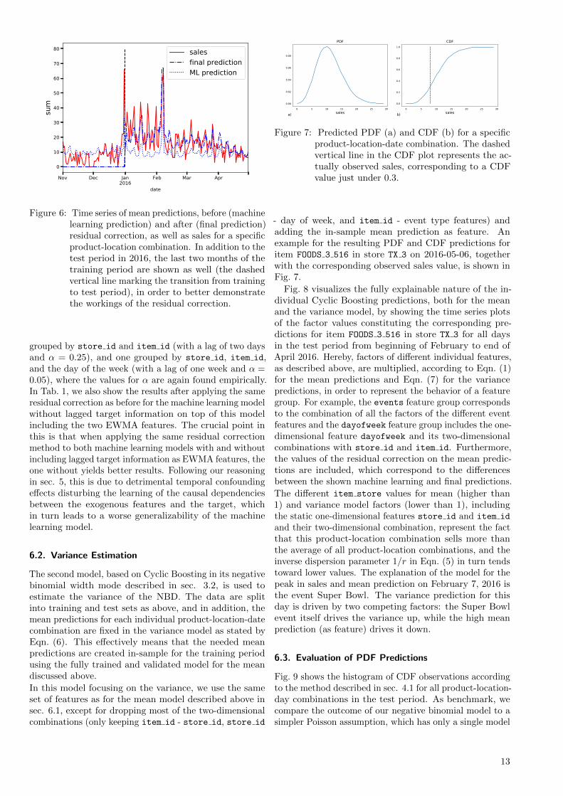
To visualize the operation principle of the residual cor-rection method, Fig. 6 shows the time series of sales and

Table 1: Accuracy metrics for the predicted mean val-ues for three different model setups: ML modelwithout lagged target information but subse-quent residual correction (a), ML model includinglagged target information by means of two EMWAfeatures without residual correction (b), and MLmodel from b) with residual correction (c).

MAD MSEa) no EWMA features,

residual correction1.65 10.09

b) EWMA features,no residual correction

1.69 10.84

c) EWMA features,residual correction

1.68 10.41

Jan2016

Feb Mar Apr May

date

2000

2250

2500

2750

3000

3250

3500

3750

4000

sum

salesfinal prediction

Figure 5: Time series of final mean predictions as well assales in test period summed over all productsand stores.

machine learning (before residual correction) as well as finalpredictions (after residual correction) for item FOODS 3 516

in store CA 3 from beginning of November 2015 to end ofApril 2016, including all days of the test period in 2016 aswell as the last two months of the training period before.Hereby, the machine learning predictions in the trainingperiod are in-sample predictions, which are just used tocalculate the residual correction. A sudden change of thesales time series at the turn of the year is visible, which isseemingly not anticipated by the machine learning model,as its predictions are clearly off in the test period in 2016.However, the residual correction is able to quickly accountfor the resulting deviations between sales and machinelearning predictions, which can be seen by the much betteragreement of the final predictions.

To give an indication of the effectiveness of the two-stepapproach, i.e., a machine learning model without laggedtarget information and residual correction as outlined insec. 5, we compare its results with a model following thecommon practice of including the lagged target informationas a variety of EMWA variables used as features in Tab. 1(for the same training and test setup). For this, we includetwo EWMA features in the machine learning model, one

12

Nov Dec Jan2016

Feb Mar Apr

date

0

10

20

30

40

50

60

70

80su

msalesfinal predictionML prediction

Figure 6: Time series of mean predictions, before (machinelearning prediction) and after (final prediction)residual correction, as well as sales for a specificproduct-location combination. In addition to thetest period in 2016, the last two months of thetraining period are shown as well (the dashedvertical line marking the transition from trainingto test period), in order to better demonstratethe workings of the residual correction.

grouped by store id and item id (with a lag of two daysand α = 0.25), and one grouped by store id, item id,and the day of the week (with a lag of one week and α =0.05), where the values for α are again found empirically.In Tab. 1, we also show the results after applying the sameresidual correction as before for the machine learning modelwithout lagged target information on top of this modelincluding the two EWMA features. The crucial point inthis is that when applying the same residual correctionmethod to both machine learning models with and withoutincluding lagged target information as EWMA features, theone without yields better results. Following our reasoningin sec. 5, this is due to detrimental temporal confoundingeffects disturbing the learning of the causal dependenciesbetween the exogenous features and the target, whichin turn leads to a worse generalizability of the machinelearning model.

6.2. Variance Estimation

The second model, based on Cyclic Boosting in its negativebinomial width mode described in sec. 3.2, is used toestimate the variance of the NBD. The data are splitinto training and test sets as above, and in addition, themean predictions for each individual product-location-datecombination are fixed in the variance model as stated byEqn. (6). This effectively means that the needed meanpredictions are created in-sample for the training periodusing the fully trained and validated model for the meandiscussed above.

In this model focusing on the variance, we use the sameset of features as for the mean model described above insec. 6.1, except for dropping most of the two-dimensionalcombinations (only keeping item id - store id, store id

0 5 10 15 20 25 30sales

0.00

0.02

0.04

0.06

0.08

a)

PDF

0 5 10 15 20 25 30sales

0.0

0.2

0.4

0.6

0.8

1.0

b)

CDF

Figure 7: Predicted PDF (a) and CDF (b) for a specificproduct-location-date combination. The dashedvertical line in the CDF plot represents the ac-tually observed sales, corresponding to a CDFvalue just under 0.3.

- day of week, and item id - event type features) andadding the in-sample mean prediction as feature. Anexample for the resulting PDF and CDF predictions foritem FOODS 3 516 in store TX 3 on 2016-05-06, togetherwith the corresponding observed sales value, is shown inFig. 7.

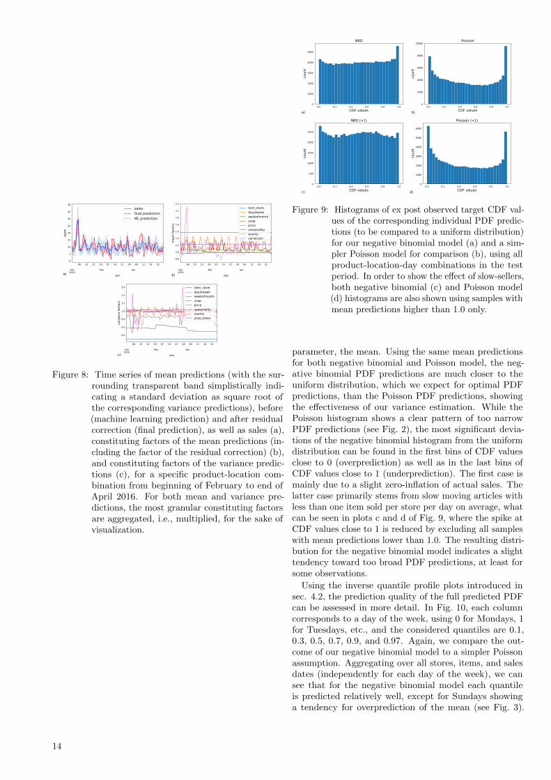
Fig. 8 visualizes the fully explainable nature of the in-dividual Cyclic Boosting predictions, both for the meanand the variance model, by showing the time series plotsof the factor values constituting the corresponding pre-dictions for item FOODS 3 516 in store TX 3 for all daysin the test period from beginning of February to end ofApril 2016. Hereby, factors of different individual features,as described above, are multiplied, according to Eqn. (1)for the mean predictions and Eqn. (7) for the variancepredictions, in order to represent the behavior of a featuregroup. For example, the events feature group correspondsto the combination of all the factors of the different eventfeatures and the dayofweek feature group includes the one-dimensional feature dayofweek and its two-dimensionalcombinations with store id and item id. Furthermore,the values of the residual correction on the mean predic-tions are included, which correspond to the differencesbetween the shown machine learning and final predictions.

The different item store values for mean (higher than1) and variance model factors (lower than 1), includingthe static one-dimensional features store id and item id

and their two-dimensional combination, represent the factthat this product-location combination sells more thanthe average of all product-location combinations, and theinverse dispersion parameter 1/r in Eqn. (5) in turn tendstoward lower values. The explanation of the model for thepeak in sales and mean prediction on February 7, 2016 isthe event Super Bowl. The variance prediction for thisday is driven by two competing factors: the Super Bowlevent itself drives the variance up, while the high meanprediction (as feature) drives it down.

6.3. Evaluation of PDF Predictions

Fig. 9 shows the histogram of CDF observations accordingto the method described in sec. 4.1 for all product-location-day combinations in the test period. As benchmark, wecompare the outcome of our negative binomial model to asimpler Poisson assumption, which has only a single model

13

Feb2016

Mar Apr

08 15 22 29 07 14 21 28 04 11 18 25

date

0

5

10

15

20

25

30

35

40

sum

a)

salesfinal predictionML prediction

Feb2016

Mar Apr

08 15 22 29 07 14 21 28 04 11 18 25

date

0.8

1.0

1.2

1.4

1.6

1.8

2.0

2.2

2.4

mea

n fa

ctor

s

b)

item_storedayofweekweekofmonthsnappriceseasonalityeventscorrection

Feb2016

Mar Apr

08 15 22 29 07 14 21 28 04 11 18 25

date

0.4

0.6

0.8

1.0

1.2

1.4

1.6

varia

nce

fact

ors

c)

item_storedayofweekweekofmonthsnappriceseasonalityeventsyhat_mean

Figure 8: Time series of mean predictions (with the sur-rounding transparent band simplistically indi-cating a standard deviation as square root ofthe corresponding variance predictions), before(machine learning prediction) and after residualcorrection (final prediction), as well as sales (a),constituting factors of the mean predictions (in-cluding the factor of the residual correction) (b),and constituting factors of the variance predic-tions (c), for a specific product-location com-bination from beginning of February to end ofApril 2016. For both mean and variance pre-dictions, the most granular constituting factorsare aggregated, i.e., multiplied, for the sake ofvisualization.

0.0 0.2 0.4 0.6 0.8 1.0CDF values

0

1000

2000

3000

4000

5000

coun

t

a)

NBD

0.0 0.2 0.4 0.6 0.8 1.0CDF values

0

2000

4000

6000

8000

10000

coun

t

b)

Poisson

0.0 0.2 0.4 0.6 0.8 1.0CDF values

0

500

1000

1500

2000

2500

coun

t

c)

NBD (>1)

0.0 0.2 0.4 0.6 0.8 1.0CDF values

0

1000

2000

3000

4000

5000

6000

coun

t

d)

Poisson (>1)

Figure 9: Histograms of ex post observed target CDF val-ues of the corresponding individual PDF predic-tions (to be compared to a uniform distribution)for our negative binomial model (a) and a sim-pler Poisson model for comparison (b), using allproduct-location-day combinations in the testperiod. In order to show the effect of slow-sellers,both negative binomial (c) and Poisson model(d) histograms are also shown using samples withmean predictions higher than 1.0 only.

parameter, the mean. Using the same mean predictionsfor both negative binomial and Poisson model, the neg-ative binomial PDF predictions are much closer to theuniform distribution, which we expect for optimal PDFpredictions, than the Poisson PDF predictions, showingthe effectiveness of our variance estimation. While thePoisson histogram shows a clear pattern of too narrowPDF predictions (see Fig. 2), the most significant devia-tions of the negative binomial histogram from the uniformdistribution can be found in the first bins of CDF valuesclose to 0 (overprediction) as well as in the last bins ofCDF values close to 1 (underprediction). The first case ismainly due to a slight zero-inflation of actual sales. Thelatter case primarily stems from slow moving articles withless than one item sold per store per day on average, whatcan be seen in plots c and d of Fig. 9, where the spike atCDF values close to 1 is reduced by excluding all sampleswith mean predictions lower than 1.0. The resulting distri-bution for the negative binomial model indicates a slighttendency toward too broad PDF predictions, at least forsome observations.

Using the inverse quantile profile plots introduced insec. 4.2, the prediction quality of the full predicted PDFcan be assessed in more detail. In Fig. 10, each columncorresponds to a day of the week, using 0 for Mondays, 1for Tuesdays, etc., and the considered quantiles are 0.1,0.3, 0.5, 0.7, 0.9, and 0.97. Again, we compare the out-come of our negative binomial model to a simpler Poissonassumption. Aggregating over all stores, items, and salesdates (independently for each day of the week), we cansee that for the negative binomial model each quantileis predicted relatively well, except for Sundays showinga tendency for overprediction of the mean (see Fig. 3).

14

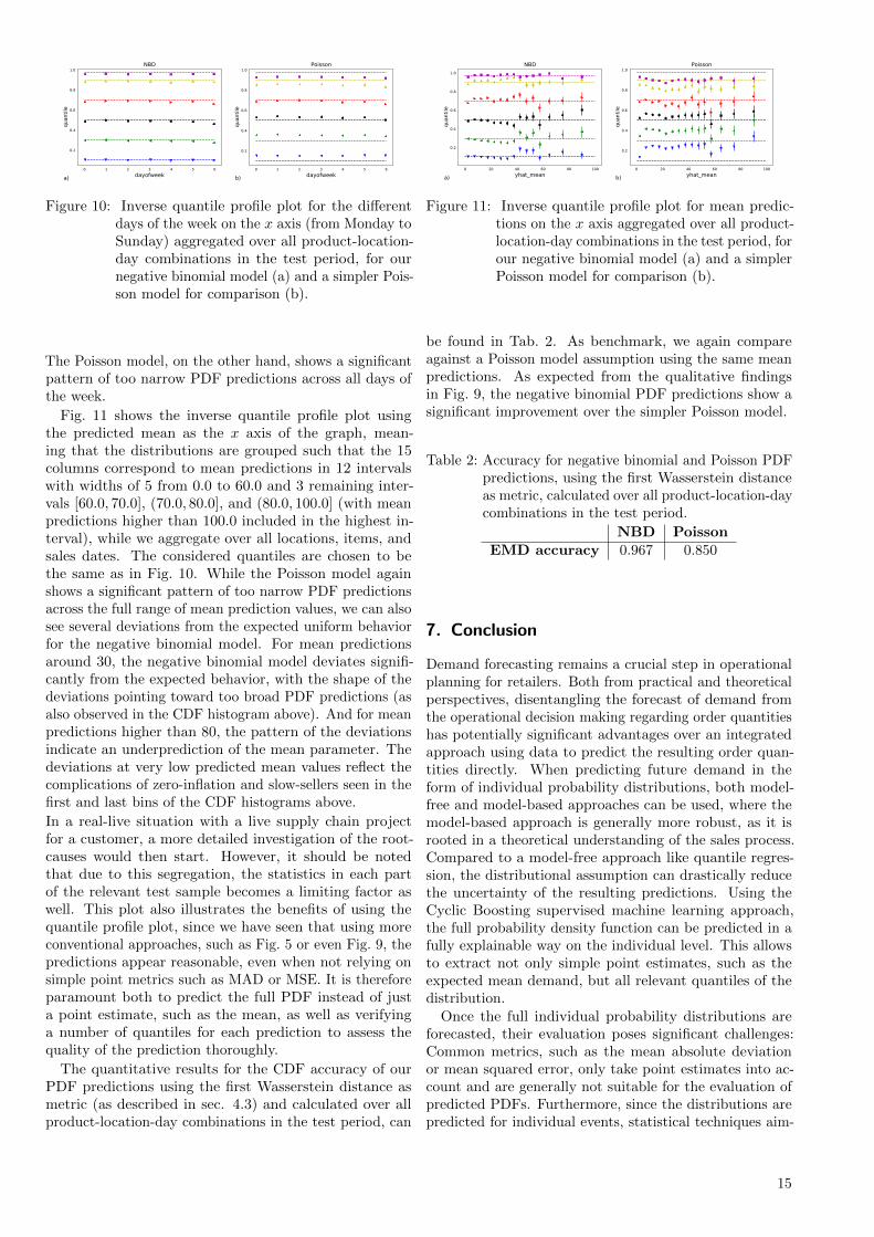
0 1 2 3 4 5 6dayofweek

0.2

0.4

0.6

0.8

1.0qu

antil

e

a)

NBD

0 1 2 3 4 5 6dayofweek

0.2

0.4

0.6

0.8

1.0

quan

tile

b)

Poisson

Figure 10: Inverse quantile profile plot for the differentdays of the week on the x axis (from Monday toSunday) aggregated over all product-location-day combinations in the test period, for ournegative binomial model (a) and a simpler Pois-son model for comparison (b).

The Poisson model, on the other hand, shows a significantpattern of too narrow PDF predictions across all days ofthe week.

Fig. 11 shows the inverse quantile profile plot usingthe predicted mean as the x axis of the graph, mean-ing that the distributions are grouped such that the 15columns correspond to mean predictions in 12 intervalswith widths of 5 from 0.0 to 60.0 and 3 remaining inter-vals [60.0, 70.0], (70.0, 80.0], and (80.0, 100.0] (with meanpredictions higher than 100.0 included in the highest in-terval), while we aggregate over all locations, items, andsales dates. The considered quantiles are chosen to bethe same as in Fig. 10. While the Poisson model againshows a significant pattern of too narrow PDF predictionsacross the full range of mean prediction values, we can alsosee several deviations from the expected uniform behaviorfor the negative binomial model. For mean predictionsaround 30, the negative binomial model deviates signifi-cantly from the expected behavior, with the shape of thedeviations pointing toward too broad PDF predictions (asalso observed in the CDF histogram above). And for meanpredictions higher than 80, the pattern of the deviationsindicate an underprediction of the mean parameter. Thedeviations at very low predicted mean values reflect thecomplications of zero-inflation and slow-sellers seen in thefirst and last bins of the CDF histograms above.

In a real-live situation with a live supply chain projectfor a customer, a more detailed investigation of the root-causes would then start. However, it should be notedthat due to this segregation, the statistics in each partof the relevant test sample becomes a limiting factor aswell. This plot also illustrates the benefits of using thequantile profile plot, since we have seen that using moreconventional approaches, such as Fig. 5 or even Fig. 9, thepredictions appear reasonable, even when not relying onsimple point metrics such as MAD or MSE. It is thereforeparamount both to predict the full PDF instead of justa point estimate, such as the mean, as well as verifyinga number of quantiles for each prediction to assess thequality of the prediction thoroughly.

The quantitative results for the CDF accuracy of ourPDF predictions using the first Wasserstein distance asmetric (as described in sec. 4.3) and calculated over allproduct-location-day combinations in the test period, can

0 20 40 60 80 100yhat_mean

0.2

0.4

0.6

0.8

1.0

quan

tile

a)

NBD

0 20 40 60 80 100yhat_mean

0.2

0.4

0.6

0.8

1.0

quan

tile

b)

Poisson

Figure 11: Inverse quantile profile plot for mean predic-tions on the x axis aggregated over all product-location-day combinations in the test period, forour negative binomial model (a) and a simplerPoisson model for comparison (b).

be found in Tab. 2. As benchmark, we again compareagainst a Poisson model assumption using the same meanpredictions. As expected from the qualitative findingsin Fig. 9, the negative binomial PDF predictions show asignificant improvement over the simpler Poisson model.

Table 2: Accuracy for negative binomial and Poisson PDFpredictions, using the first Wasserstein distanceas metric, calculated over all product-location-daycombinations in the test period.

NBD PoissonEMD accuracy 0.967 0.850

7. Conclusion

Demand forecasting remains a crucial step in operationalplanning for retailers. Both from practical and theoreticalperspectives, disentangling the forecast of demand fromthe operational decision making regarding order quantitieshas potentially significant advantages over an integratedapproach using data to predict the resulting order quan-tities directly. When predicting future demand in theform of individual probability distributions, both model-free and model-based approaches can be used, where themodel-based approach is generally more robust, as it isrooted in a theoretical understanding of the sales process.Compared to a model-free approach like quantile regres-sion, the distributional assumption can drastically reducethe uncertainty of the resulting predictions. Using theCyclic Boosting supervised machine learning approach,the full probability density function can be predicted in afully explainable way on the individual level. This allowsto extract not only simple point estimates, such as theexpected mean demand, but all relevant quantiles of thedistribution.

Once the full individual probability distributions areforecasted, their evaluation poses significant challenges:Common metrics, such as the mean absolute deviationor mean squared error, only take point estimates into ac-count and are generally not suitable for the evaluation ofpredicted PDFs. Furthermore, since the distributions arepredicted for individual events, statistical techniques aim-

15

ing at the comparison of distributions using many eventscannot be used in general. Instead, novel techniques ex-ploiting the probability integral transform, namely thehistogram of observed CDF values of the predicted indi-vidual PDFs as well as inverse quantile profile plots, allowa detailed investigation into the behavior of the predic-tions. Finally, a quantitative assessment resulting in asingle number can be obtained using metrics such as theearth mover distance in a comparison between the his-togram of observed CDF values and the expected uniformdistribution.

An additional challenge for demand forecasting in spe-cific and time series forecasting in general is the handlingof the detrimental effects of temporal confounding, es-pecially on explainability and generalizability of the em-ployed models. Using a two-step model consisting of amachine learning model, including all available exogenousvariables as features but excluding any lagged target in-formation, to control for all known temporal confounders,and a subsequent empiric residual correction to captureany information on recent trends missed in the machinelearning model, temporal confounding can be avoided, orat least mitigated.

References

[1] F. Edgeworth, The Mathematical Theory of BankingJournal of the Royal Statistical Society, 1888.

[2] M. Khouja, The single-period (news-vendor) problem:literature review and suggestions for future researchOmega, vol. 27, no. 5, pp. 537–553, 1999.

[3] F. Wick, U. Kerzel, and M. Feindt, Cyclic Boosting -An Explainable Supervised Machine Learning Algo-rithm in 2019 18th IEEE International ConferenceOn Machine Learning And Applications (ICMLA),pp. 358–363, IEEE, 12 2019.

[4] Statista, Profit margin of Lidl Sverige from 2013 to2015 https://www.statistia.com/statistics/

779146/profit-margin-of-lidl-sverige/ (lastaccessed: 2020-Dec-01).

[5] Statista, Operating margin of Willysin Sweden from 2012 to 2018 https:

//www.statistia.com/statistics/734261/

operating-margin-of-willys-in-sweden/ (lastaccessed: 2020-Dec-01).

[6] Statista, Operating margin of Hemkopin Sweden from 2012 to 2018 https:

//www.statistia.com/statistics/734370/

operating-margin-of-hemkoep-in-sweden/

(last accessed: 2020-Dec-01).

[7] Statista, Operating profit margin of Publix Su-per Markets in the United States from 2017 to2019 https://www.statistia.com/statistics/

1167301/publix-operating-profit-us/ (last ac-cessed: 2020-Dec-01).

[8] S. Beheshti-Kashi, H. R. Karimi, K.-D. Thoben,M. Lutjen, and M. Teucke, A survey on retail salesforecasting and prediction in fashion markets Sys-tems Science & Control Engineering, vol. 3, no. 1,pp. 154–161, 2015.

[9] G. E. P. Box, G. M. Jenkins, G. C. Reinsel, andG. M. Ljungl, Time Series Analysis: Forecasting andControl. Wiley, 5 ed., 2015.

[10] J. D. Croston, Forecasting and stock control for inter-mittent demands Journal of the Operational ResearchSociety, vol. 23, no. 3, pp. 289–303, 1972.

[11] C. C. Holt, Forecasting trends and seasonal by expo-nentially weighted moving averages ONR Memoran-dum, vol. 52, 1957.

[12] R. G. Brown, Smoothing Forecasting and Predictionof Discrete Time Series. Prentice-Hall International,Inc. London, UK, 1963.

[13] E. S. Gardner, Exponential smoothing: the state ofthe art Journal of Forecasting, vol. 4, pp. 1–28, 1985.

[14] J. G. De Gooijer and R. J. Hyndman, 25 years of timeseries forecasting International journal of forecasting,vol. 22, no. 3, pp. 443–473, 2006.

[15] J. Huber, A. Gossmann, and H. Stuckenschmidt,Cluster-based hierarchical demand forecasting for per-ishable goods Expert systems with applications, vol. 76,pp. 140–151, 2017.

[16] M. Kalchschmidt, R. Verganti, and G. Zotteri, Fore-casting demand from heterogeneous customers Inter-national Journal of operations & Production manage-ment, 2006.

[17] J. Fattah, L. Ezzine, Z. Aman, H. El Moussami, andA. Lachhab, Forecasting of demand using ARIMAmodel International Journal of Engineering BusinessManagement, vol. 10, p. 1847979018808673, 2018.

[18] C. I. Permatasari, W. Sutopo, and M. Hisjam, Salesforecasting newspaper with ARIMA: A case studyin AIP Conference Proceedings, vol. 1931, p. 030017,AIP Publishing LLC, 2018.

[19] R. E. Kalman, A new approach to linear filtering andprediction problems Journal of Basic Engineering,vol. 82, no. 1, pp. 35–45, 1960.

[20] G. W. Morrison and D. H. Pike, Kalman filteringapplied to statistical forecasting Management Science,vol. 23, no. 7, pp. 768–774, 1977.

[21] C. Mitropoulos, J. Samouilidis, and E. Protonotarios,Using Kalman Filtering for Energy Forecasting IFACProceedings Volumes, vol. 13, no. 5, pp. 317–324, 1980.

[22] A. Tegene, Kalman filter and the demand forcigarettes Applied Economics, vol. 23, no. 7, pp. 1175–1182, 1991.

16

[23] K. Kandananond, Applying Kalman Filter for Corre-lated Demand Forecasting in Applied Mechanics andMaterials, vol. 619, pp. 381–384, Trans Tech Publ,2014.

[24] M. Jacobi, D. Karimanzira, and C. Ament, Waterdemand forecasting using Kalman filtering in Proceed-ings of the 16th IASTED International Conference onApplied Simulation and Modelling, pp. 199–202, 2007.

[25] R. Hyndman, A. B. Koehler, J. K. Ord, and R. D.Snyder, Forecasting with exponential smoothing: thestate space approach. Springer Science & BusinessMedia, 2008.

[26] P. Ramos, N. Santos, and R. Rebelo, Performance ofstate space and ARIMA models for consumer retailsales forecasting Robotics and computer-integratedmanufacturing, vol. 34, pp. 151–163, 2015.

[27] A. Harvey and S. Peters, Estimation procedures forstructural time series models Journal of Forecasting,vol. 9, pp. 89–108, 1990.

[28] S. J. Taylor and B. Letham, Forecasting at scale TheAmerican Statistician, vol. 72, no. 1, pp. 37–45, 2018.

[29] A. G. Kok and M. L. Fisher, Demand estimation andassortment optimization under substitution: Method-ology and application Operations Research, vol. 55,no. 6, pp. 1001–1021, 2007.

[30] H.-J. Wang, C.-F. Chien, and C.-F. Liu, DemandForecasting Using Bayesian Experiment with Non-homogenous Poisson Process Model InternationalJournal of Operations Research, vol. 2, no. 1, pp. 21–29, 2005.

[31] G. Zhang, Neural Networks for time-series forecasting,pp. 461–477. Springer Berlin, Heidelberg, 2012.

[32] W. Remus and M. O’Connor, Neural networks fortime-series forecasting in Principles of forecasting,pp. 245–256, Springer, 2001.

[33] L. Breiman, J. Friedman, C. J. Stone, and R. A.Olshen, Classification and regression trees. CRC press,1984.

[34] K. J. Ferreira, B. H. A. Lee, and D. Simchi-Levi, An-alytics for an online retailer: Demand forecasting andprice optimization Manufacturing & Service Opera-tions Management, vol. 18, no. 1, pp. 69–88, 2016.

[35] D. Rumelhart, G. Hinton, and R. Williams, Learningrepresentations by back-propagating errors Nature,vol. 323, pp. 533–536, 1986.

[36] S. Hochreiter and J. Schmidhuber, Long short-termmemory Neural computation, vol. 9, no. 8, pp. 1735–1780, 1997.

[37] A. Vaswani, N. Shazeer, N. Parmar, J. Uszkoreit,L. Jones, A. N. Gomez, L. u. Kaiser, and I. Polo-sukhin, Attention is All you Need in Advances inNeural Information Processing Systems 30 (I. Guyon,

U. V. Luxburg, S. Bengio, H. Wallach, R. Fergus,S. Vishwanathan, and R. Garnett, eds.), pp. 5998–6008, Curran Associates, Inc., 2017.

[38] K. Bandara, P. Shi, C. Bergmeir, H. Hewamalage,Q. Tran, and B. Seaman, Sales demand forecast ine-commerce using a long short-term memory neuralnetwork methodology in International Conference onNeural Information Processing, pp. 462–474, Springer,2019.

[39] Q. Yu, K. Wang, J. O. Strandhagen, and Y. Wang,Application of long short-term memory neural net-work to sales forecasting in retail—a case study inInternational Workshop of Advanced Manufacturingand Automation, pp. 11–17, Springer, 2017.

[40] A. Goyal, R. Kumar, S. Kulkarni, S. Krishnamurthy,and M. Vartak, A solution to forecast demand usinglong short-term memory recurrent neural networks fortime series forecasting in Midwest Decision SciencesInstitute Conference, 2018.

[41] S. Helmini, N. Jihan, M. Jayasinghe, and S. Per-era, Sales forecasting using multivariate long shortterm memory network models PeerJ PrePrints, vol. 7,p. e27712v1, 2019.

[42] M. Golkabek, R. Senge, and R. Neumann, DemandForecasting using Long Short-Term Memory NeuralNetworks arXiv preprint arXiv:2008.08522, 2020.

[43] M. Langkvist, L. Karlsson, and A. Loutfi, A reviewof unsupervised feature learning and deep learningfor time-series modeling Pattern Recognition Letters,vol. 42, pp. 11–24, 2014.

[44] M. F. Dixon, Industrial Forecasting with Exponen-tially Smoothed Recurrent Neural Networks arXivpreprint arXiv:2004.04717, 2020.

[45] I. Goodfellow, J. Pouget-Abadie, M. Mirza, B. Xu,D. Warde-Farley, S. Ozair, A. Courville, and Y. Ben-gio, Generative adversarial nets in Advances in neuralinformation processing systems, pp. 2672–2680, 2014.

[46] M. Haas and S. Richter, Statistical analysis of Wasser-stein GANs with applications to time series forecastingarXiv preprint arXiv:2011.03074, 2020.

[47] G. Ramponi, P. Protopapas, M. Brambilla, andR. Janssen, T-cgan: Conditional generative ad-versarial network for data augmentation in noisytime series with irregular sampling arXiv preprintarXiv:1811.08295, 2018.

[48] K. E. Smith and A. O. Smith, ConditionalGAN for timeseries generation arXiv preprintarXiv:2006.16477, 2020.

[49] D. Malinsky and P. Spirtes, Causal structure learn-ing from multivariate time series in settings withunmeasured confounding in Proceedings of 2018 ACMSIGKDD Workshop on Causal Discovery, pp. 23–47,2018.

17

[50] J. Runge, Causal network reconstruction from timeseries: From theoretical assumptions to practical esti-mation Chaos: An Interdisciplinary Journal of Non-linear Science, vol. 28, no. 7, p. 075310, 2018.

[51] J. Runge, P. Nowack, M. Kretschmer, S. Flaxman,and D. Sejdinovic, Detecting and quantifying causalassociations in large nonlinear time series datasetsScience Advances, vol. 5, p. eaau4996, Nov 2019.

[52] I. Bica, A. Alaa, and M. Van Der Schaar, Time seriesdeconfounder: Estimating treatment effects over timein the presence of hidden confounders in InternationalConference on Machine Learning, pp. 884–895, PMLR,2020.

[53] K. Perrakis, A. Gryparis, J. Schwartz, A. L. Tertre,K. Katsouyanni, F. Forastiere, M. Stafoggia, andE. Samoli, Controlling for seasonal patterns and timevarying confounders in time-series epidemiologicalmodels: a simulation study Statistics in medicine,vol. 33, no. 28, pp. 4904–4918, 2014.

[54] K. H. Brodersen, F. Gallusser, J. Koehler, N. Remy,and S. L. Scott, Inferring causal impact using Bayesianstructural time-series models Annals of Applied Statis-tics, vol. 9, pp. 247–274, 2015.

[55] K. H. Brodersen and A. Hauser, “CausalImpact: AnR package for causal inference in time series.” http://

google.github.io/CausalImpact/. (last accessed:2020-Dec-19).

[56] C. Chatfield, Calculating interval forecasts Journalof Business & Economic Statistics, vol. 11, no. 2,pp. 121–135, 1993.

[57] G. Masarotto, Bootstrap prediction intervals for au-toregressions International Journal of Forecasting,vol. 6, no. 2, pp. 229–239, 1990.

[58] B. McCullough, Bootstrapping forecast intervals: anapplication to AR(p) models Journal of Forecasting,vol. 13, no. 1, pp. 51–66, 1994.

[59] B. McCullough, Consistent forecast intervals whenthe forecast-period exogenous variables are stochasticJournal of Forecasting, vol. 15, no. 4, pp. 293–304,1996.

[60] M. Grigoletto, Bootstrap prediction intervals for au-toregressions: some alternatives International Journalof Forecasting, vol. 14, no. 4, pp. 447–456, 1998.

[61] L. A. Thombs and W. R. Schucany, Bootstrap pre-diction intervals for autoregression Journal of theAmerican Statistical Association, vol. 85, no. 410,pp. 486–492, 1990.

[62] M. P. Clements and N. Taylor, Bootstrapping predic-tion intervals for autoregressive models InternationalJournal of Forecasting, vol. 17, no. 2, pp. 247–267,2001.

[63] J. E. Angus, The Probability Integral Transform andRelated Results SIAM Review, vol. 36, no. 4, pp. 652–654, 1994.

[64] L. Pascual, J. Romo, and E. Ruiz, Bootstrap predic-tive inference for ARIMA processes Journal of TimeSeries Analysis, vol. 25, no. 4, pp. 449–465, 2004.

[65] L. Pascual, J. Romo, and E. Ruiz, Effects of param-eter estimation on prediction densities: a bootstrapapproach International Journal of Forecasting, vol. 17,no. 1, pp. 83–103, 2001.

[66] L. Pascual, J. Romo, and E. Ruiz, Bootstrap pre-diction intervals for power-transformed time seriesInternational Journal of Forecasting, vol. 21, no. 2,pp. 219–235, 2005.

[67] R. Koenker and K. F. Hallock, Quantile regres-sion Journal of economic perspectives, vol. 15, no. 4,pp. 143–156, 2001.

[68] M. Feindt and U. Kerzel, The NeuroBayes neuralnetwork package NIM A, vol. 559, no. 1, pp. 190–194,2006.

[69] R. J. Hyndman, Highest-density forecast regions fornonlinear and non-normal time series models Journalof Forecasting, vol. 14, no. 5, pp. 431–441, 1995.

[70] A. S. Tay and K. F. Wallis, Density forecasting: asurvey Journal of forecasting, vol. 19, no. 4, pp. 235–254, 2000.

[71] R. Wen, K. Torkkola, B. Narayanaswamy, andD. Madeka, A multi-horizon quantile recurrent fore-caster arXiv preprint arXiv:1711.11053, 2017.

[72] B. Lim, S. O. Arik, N. Loeff, and T. Pfis-ter, Temporal fusion transformers for interpretablemulti-horizon time series forecasting arXiv preprintarXiv:1912.09363, 2019.

[73] D. J. Rezende and S. Mohamed, Variational In-ference with Normalizing Flows arXiv preprintarXiv:1505.05770, 2015.

[74] K. Rasul, A.-S. Sheikh, I. Schuster, U. Bergmann, andR. Vollgraf, Multi-variate Probabilistic Time SeriesForecasting via Conditioned Normalizing Flows arXivpreprint arXiv:2002.06103, 2020.

[75] C. M. Bishop, “Mixture density networks.” http:

//publications.aston.ac.uk/id/eprint/373/,1994.

[76] D. Salinas, V. Flunkert, J. Gasthaus, andT. Januschowski, DeepAR: Probabilistic forecastingwith autoregressive recurrent networks InternationalJournal of Forecasting, vol. 36, no. 3, pp. 1181–1191,2020.

[77] I. Adan, M. van Eenige, and J. Resing, Fitting discretedistributions on the first two moments Probability inthe engineering and informational sciences, vol. 9,no. 4, pp. 623–632, 1995.

18

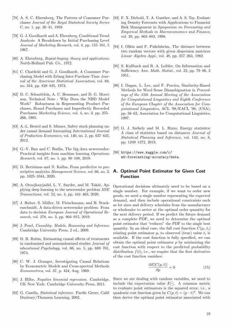
[78] A. S. C. Ehrenberg, The Pattern of Consumer Pur-chases Journal of the Royal Statistical Society SeriesC, no. 1, pp. 26–41, 1959.

[79] G. J. Goodhardt and A. Ehrenberg, Conditional TrendAnalysis: A Breakdown by Initial Purchasing LevelJournal of Marketing Research, vol. 4, pp. 155–161, 51967.

[80] A. Ehrenberg, Repeat-buying; theory and applications.North-Holland Pub. Co., 1972.

[81] C. Chatfield and G. J. Goodhardt, A Consumer Pur-chasing Model with Erlang Inter-Purchase Time Jour-nal of the American Statistical Association, vol. 68,no. 344, pp. 828–835, 1973.

[82] D. C. Schmittlein, A. C. Bemmaor, and D. G. Morri-son, Technical Note - Why Does the NBD ModelWork? Robustness in Representing Product Pur-chases, Brand Purchases and Imperfectly RecordedPurchases Marketing Science, vol. 4, no. 3, pp. 255–266, 1985.

[83] A.-L. Beutel and S. Minner, Safety stock planning un-der causal demand forecasting International Journalof Production Economics, vol. 140, no. 2, pp. 637–645,2012.

[84] G.-Y. Ban and C. Rudin, The big data newsvendor:Practical insights from machine learning OperationsResearch, vol. 67, no. 1, pp. 90–108, 2019.

[85] D. Bertsimas and N. Kallus, From predictive to pre-scriptive analytics Management Science, vol. 66, no. 3,pp. 1025–1044, 2020.

[86] A. Oroojlooyjadid, L. V. Snyder, and M. Takac, Ap-plying deep learning to the newsvendor problem IISETransactions, vol. 52, no. 4, pp. 444–463, 2020.

[87] J. Huber, S. Muller, M. Fleischmann, and H. Stuck-enschmidt, A data-driven newsvendor problem: Fromdata to decision European Journal of Operational Re-search, vol. 278, no. 3, pp. 904–915, 2019.

[88] J. Pearl, Causality: Models, Reasoning and Inference.Cambridge University Press, 2 ed., 2009.

[89] D. B. Rubin, Estimating causal effects of treatmentsin randomized and nonrandomized studies Journal ofeducational Psychology, vol. 66, no. 5, pp. 688–701,1974.

[90] C. W. J. Granger, Investigating Causal Relationsby Econometric Models and Cross-spectral MethodsEconometrica, vol. 37, p. 424, Aug. 1969.

[91] J. Hilbe, Negative binomial regression. Cambridge,UK New York: Cambridge University Press, 2011.

[92] G. Casella, Statistical inference. Pacific Grove, Calif:Duxbury/Thomson Learning, 2002.

[93] F. X. Diebold, T. A. Gunther, and A. S. Tay, Evaluat-ing Density Forecasts with Applications to FinancialRisk Management in Symposium on Forecasting andEmpirical Methods in Macroeconomics and Finance,vol. 39, pp. 863–883, 1998.

[94] I. Olkin and F. Pukelsheim, The distance betweentwo random vectors with given dispersion matricesLinear Algebra Appl., vol. 48, pp. 257–263, 1982.

[95] S. Kullback and R. A. Leibler, On Information andSufficiency Ann. Math. Statist., vol. 22, pp. 79–86, 31951.

[96] I. Dagan, L. Lee, and F. Pereira, Similarity-BasedMethods for Word Sense Disambiguation in Proceed-ings of the 35th Annual Meeting of the Associationfor Computational Linguistics and Eighth Conferenceof the European Chapter of the Association for Com-putational Linguistics, ACL ’98/EACL ’98, (USA),pp. 56–63, Association for Computational Linguistics,1997.

[97] G. J. Szekely and M. L. Rizzo, Energy statistics:A class of statistics based on distances Journal ofStatistical Planning and Inference, vol. 143, no. 8,pp. 1249–1272, 2013.

[98] https://www.kaggle.com/c/

m5-forecasting-accuracy/data.

A. Optimal Point Estimator for Given CostFunction

Operational decisions ultimately need to be based on asingle number. For example, if we want to order newgoods, we need a single number representing the expecteddemand, and then include operational constraints suchas lot sizes and delivery schedules from the manufactureror wholesaler to arrive at the optimal order quantity forthe next delivery period. If we predict the future demandas a complete PDF, we need to determine the optimalpoint estimator that “reduces” the PDF to the single bestquantity. In an ideal case, the full cost function C(pi, ti)relating point estimator pi to observed (true) value ti isavailable. If the cost function is fully specified, we canobtain the optimal point estimator p by minimizing thecost function with respect to the predicted probabilitydistribution f(t), i.e., we require that the first derivativeof the cost function vanishes:

∂E[C(p, t)]

∂p= 0 (15)

Since we are dealing with random variables, we need toinclude the expectation value E[·]. A common metricto evaluate point estimators is the squared error, i.e., aquadratic cost function given by C(p, t) = (p− t)2. We canthen derive the optimal point estimator associated with

19

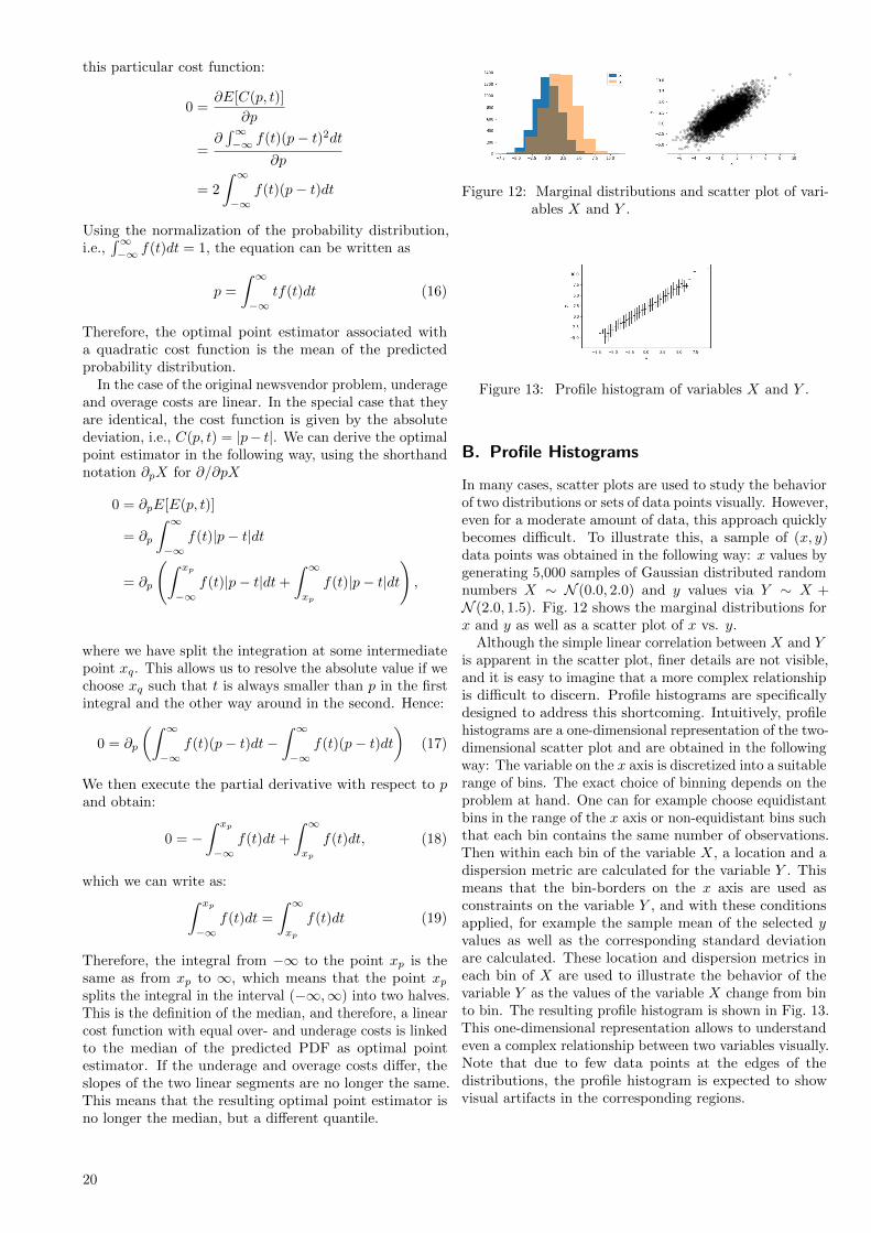
this particular cost function:

0 =∂E[C(p, t)]

∂p

=∂∫∞−∞ f(t)(p− t)2dt

∂p

= 2

∫ ∞−∞

f(t)(p− t)dt

Using the normalization of the probability distribution,i.e.,

∫∞−∞ f(t)dt = 1, the equation can be written as

p =

∫ ∞−∞

tf(t)dt (16)

Therefore, the optimal point estimator associated witha quadratic cost function is the mean of the predictedprobability distribution.

In the case of the original newsvendor problem, underageand overage costs are linear. In the special case that theyare identical, the cost function is given by the absolutedeviation, i.e., C(p, t) = |p− t|. We can derive the optimalpoint estimator in the following way, using the shorthandnotation ∂pX for ∂/∂pX

0 = ∂pE[E(p, t)]

= ∂p

∫ ∞−∞

f(t)|p− t|dt

= ∂p

(∫ xp

−∞f(t)|p− t|dt+

∫ ∞xp

f(t)|p− t|dt

),

where we have split the integration at some intermediatepoint xq. This allows us to resolve the absolute value if wechoose xq such that t is always smaller than p in the firstintegral and the other way around in the second. Hence:

0 = ∂p

(∫ ∞−∞

f(t)(p− t)dt−∫ ∞−∞

f(t)(p− t)dt)

(17)

We then execute the partial derivative with respect to pand obtain:

0 = −∫ xp

−∞f(t)dt+

∫ ∞xp

f(t)dt, (18)

which we can write as:∫ xp

−∞f(t)dt =

∫ ∞xp

f(t)dt (19)

Therefore, the integral from −∞ to the point xp is thesame as from xp to ∞, which means that the point xpsplits the integral in the interval (−∞,∞) into two halves.This is the definition of the median, and therefore, a linearcost function with equal over- and underage costs is linkedto the median of the predicted PDF as optimal pointestimator. If the underage and overage costs differ, theslopes of the two linear segments are no longer the same.This means that the resulting optimal point estimator isno longer the median, but a different quantile.

Figure 12: Marginal distributions and scatter plot of vari-ables X and Y .

Figure 13: Profile histogram of variables X and Y .

B. Profile Histograms

In many cases, scatter plots are used to study the behaviorof two distributions or sets of data points visually. However,even for a moderate amount of data, this approach quicklybecomes difficult. To illustrate this, a sample of (x, y)data points was obtained in the following way: x values bygenerating 5,000 samples of Gaussian distributed randomnumbers X ∼ N (0.0, 2.0) and y values via Y ∼ X +N (2.0, 1.5). Fig. 12 shows the marginal distributions forx and y as well as a scatter plot of x vs. y.

Although the simple linear correlation between X and Yis apparent in the scatter plot, finer details are not visible,and it is easy to imagine that a more complex relationshipis difficult to discern. Profile histograms are specificallydesigned to address this shortcoming. Intuitively, profilehistograms are a one-dimensional representation of the two-dimensional scatter plot and are obtained in the followingway: The variable on the x axis is discretized into a suitablerange of bins. The exact choice of binning depends on theproblem at hand. One can for example choose equidistantbins in the range of the x axis or non-equidistant bins suchthat each bin contains the same number of observations.Then within each bin of the variable X, a location and adispersion metric are calculated for the variable Y . Thismeans that the bin-borders on the x axis are used asconstraints on the variable Y , and with these conditionsapplied, for example the sample mean of the selected yvalues as well as the corresponding standard deviationare calculated. These location and dispersion metrics ineach bin of X are used to illustrate the behavior of thevariable Y as the values of the variable X change from binto bin. The resulting profile histogram is shown in Fig. 13.This one-dimensional representation allows to understandeven a complex relationship between two variables visually.Note that due to few data points at the edges of thedistributions, the profile histogram is expected to showvisual artifacts in the corresponding regions.

20