NBER WORKING PAPER SERIES

RATINGS AND ASSET ALLOCATION:AN EXPERIMENTAL ANALYSIS

Robert L. McDonaldThomas A. Rietz

Working Paper 25046http://www.nber.org/papers/w25046

NATIONAL BUREAU OF ECONOMIC RESEARCH1050 Massachusetts Avenue

Cambridge, MA 02138September 2018

We thank the TIAA-CREF Institute for funding this research and Ying Xu for programming. For helpful comments we also thank Bruno Biais, Craig Furfine, Simon Gervais, Luigi Guiso, Ravi Jagannathan, Lisa Kramer, Cami Kuhnen, Owen Lamont, Daniel Martin, Olivia Mitchell, Brian Sternthal, Tom Vinaimont, seminar participants at the New York Fed, Northwestern University, University of Iowa, University of Illinois, City University of Hong Kong, Hong Kong University, Hong Kong Polytechnic University, Korea University Business School, and conference participants at the Economic Science Association meetings, UBC, and the Wharton Conference on Household Finance. The views expressed herein are those of the authors and do not necessarily reflect the views of the National Bureau of Economic Research.

NBER working papers are circulated for discussion and comment purposes. They have not been peer-reviewed or been subject to the review by the NBER Board of Directors that accompanies official NBER publications.

© 2018 by Robert L. McDonald and Thomas A. Rietz. All rights reserved. Short sections of text, not to exceed two paragraphs, may be quoted without explicit permission provided that full credit, including © notice, is given to the source.

Ratings and Asset Allocation: An Experimental AnalysisRobert L. McDonald and Thomas A. RietzNBER Working Paper No. 25046September 2018JEL No. G4,G41

ABSTRACT

Investment ratings (e.g., by Morningstar) provide a simple ordinal scale (e.g., 1 to 5) for comparing investments. Typically, ratings are assigned within categories — groups of assets sharing common characteristics — but using the same ordinal scale for all groups. Comparing such categorized ratings across categories is potentially misleading. We study the effect of categorized ratings in an asset allocation experiment in which subjects make repeated allocation decisions under complete information. Subjects initially see no ratings, and they then see either categorized or uncategorized ratings. Although ratings convey no information, categorized ratings affect subject investment choices and harm performance in the experiment. Subjects do not simply invest more in highly rated assets. Rather, rating effects seem to occur when ratings conflict with subjects’ own evaluation of assets: subjects reduce their investment in a high quality asset which receives an intermediate rating, but they do not increase their investment in a high-quality asset that receives a high rating. Knowledge and experience help with the base allocation task but do not mitigate the harmful effect of categorized ratings.

Robert L. McDonaldKellogg School of ManagementNorthwestern University2211 Campus DrEvanston, IL 60208and NBERr-mcdonald@northwestern.edu

Thomas A. RietzDepartment of Finance, S244PBBUniversity of IowaIowa City, Iowa 52242-1994thomas-rietz@uiowa.edu

1 Introduction

Personal financial decisions are complicated and have ramifications that span decades. Investors

face a variety of long-term risks and are confronted with numerous assets and investment strategies.

Fully optimal portfolio decisions that take into account realistic extensions to the basic model

(factoring in uncertain labor income, for example) are complicated in all but the simplest cases

(e.g., see Merton, 1971, 1973).

Many advisory firms provide asset and fund ratings to assist investors in making investment

decisions.1 These ratings are often assigned within investment categories, with the implication

that ratings are comparable within a category but not across categories. In 2016, for example,

Morningstar assigned funds to 122 distinct categories, with funds in each category rated using one

to five stars (worst to best), and with stars assigned using a mandatory curve based on risk-adjusted

historical returns.2 Because of the mandatory curve, the star rating is not absolute: a fund’s star

rating can change when other funds enter or leave the category. More importantly, the star rating

is not investment advice, as an investor’s optimal allocation decisions should depend on a fund’s

contribution to the return and risk for the investor’s entire portfolio. In particular, comparing funds

across investment categories makes little sense: a 5-star fund in “Equity Precious Metals” cannot

be directly compared to a 3-star fund in “Corporate Bonds.” Categorized ratings are thus double-

edged: they compare performance to other investments of a similar style, but the use of a common

scale across categories may distort choices by making non-comparable items appear comparable.

Credit ratings create a similar issue. Rating agencies use a familiar ordinal system (AAA,

AA, etc.) to describe the credit risk of both bonds and structured products, even though ratings

are not meant to be comparable across categories. Similar examples include movie ratings, wine

ratings, and nutrition ratings, for all of which consumption decisions entail both within-category

and across-cateogry comparisons.

We report on an experiment designed to assess the effects of such categorized ratings. In a

setting with complete information about asset characteristics, subjects allocate money across six

investment alternatives, in multiple trials. Each of the investments has a binomial payoff that is

perfectly correlated across the assets. Subjects have complete information about the assets at all

1Advisory firms supplying ratings include CFRA, Lipper, Morningstar, TheStreet, and Zacks. US News averagesthese five ratings to supply its own rating.

2Ten percent of funds in each category receive 5 stars and 1 star each, 22.5% receive 4 and 2 stars each, and 35%receive three stars. The original Morningstar ranking system was introduced in 1985, with all stock funds rankedin a common pool (Blume, 1998). In 1996, category rankings were introduced. In 2002, smaller category groupswere introduced (Morningstar, 2008). Morningstar justified categorization as eliminating a “tail-wind” effect, inwhich specific industries or investment styles would by chance generate high returns and receive investor attention.By eliminating one problem, however, categorization could create a different problem, creating the appearance ofcomparability where there is none.

1

times: the presentation in each trial includes the high and low returns for each investment, along

with the mean return, range, and the return/range ratio. In comparing assets, therefore, subjects

do not have to perform computations, think about diversification, or remember asset characteristics

from one trial to the next. This design eliminates many computational and cognitive hurdles for

subjects, and was motivated by the existing literature showing that individuals have limitations

and behavioral biases in perception, attention, and cognitive ability. Payoffs are revealed at the

conclusion of the experiment, so there is no learning about returns, statistical inference, or income

effect. Risk-averse investors should have an unambiguous preference for two of the assets; of the

remaining four, two would only be optimal for risk seeking subjects and two have payoffs that are

strictly dominated for any risk preference. Diversification across the six assets is suboptimal.

The main treatment is categorization. In the first trial, the assets have no ratings. Subjects

are then shown star ratings, with half of subjects shown uncategorized ratings and the other half

shown categorized ratings. Categorization alters the rating of four of the six assets, and reduces the

rating of one of the assets that should be preferred by risk-averse subjects. We find that subjects

exposed to categorized ratings hold less of the lower-rated optimal asset, and as a result perform

more poorly. At the end of the experiment, subjects take a financial knowledge quiz, allowing us

to correlate the knowledge score with behavior. Knowledgable subjects perform better but are still

affected by categorization.

Subjects could be influenced by ratings for different reasons. One possibility is the experimenter-

demand effect (Zizzo, 2010), in which subjects respond to a cue such as star ratings because they

believe they are supposed to do so. An alternative is that subjects are cognitively challenged, have

difficulty with the experimental task, and use the ratings to assist them in decision-making. A third

possibility is that subjects face cognitive dissonance when a rating is inconsistent with their prior

belief about the asset and they respond to this dissonance by investing less, thereby harmonizing

the rating and their behavior.

While all three explanations seem plausible, subject behavior does not align with the first two.

Subjects perform reasonably well in the allocation task without ratings, suggesting cognitive ability

with the task. When shown ratings, subjects do not change investment behavior on average except

in the case where ratings are altered by categorization. In this case, ratings affect choices when

ratings conflict with subjects’ own evaluation of assets: subjects reduce their investment in a high

quality asset which receives an intermediate rating, but they do not increase their investment in

a high-quality asset that receives a high rating. This seems to rule out the experimenter demand

effect, which in its strongest form would predict that subjects going from no stars to stars would

invest more heavily in the highest rated assets and less in the lower-rated. The likeliest explanation

seems to be dissonance stemming from the inconsistency of categorized ratings with the belief about

2

asset quality.

While we defer a detailed discussion of the related literature until after we have presented our

results, we note that the experiment touches on four distinct but related questions that have been

discussed in the literature:

• How does the presentation of summary information and investment alternatives affect invest-

ment choices? This has been studied in the context of Morningstar ratings (Del Guercio and

Tkac, 2008; Reuter and Zitzewitz, 2015), bond ratings (Chen et al., 2014), and in the study

of menu effects (Bateman et al., 2016; Benartzi and Thaler, 2001; Huberman and Jiang, 2006;

Massa et al., 2015).3

• How do financial knowledge and experience affect investment behavior? Bernheim et al.

(2001), Bernheim and Garrett (2003), Lusardi and Mitchell (2007), and Anderson and Settle

(1996) all demonstrate effects of financial literacy.

• How do cognitive limitations affect decision making (Edgell et al., 1996; Thaler, 1980; Tversky

and Kahneman, 1974; Camerer et al., 1989)?

• Can subjects make appropriate portfolio choice decisions (Moore et al., 1999; Kroll et al.,

1988, 2003)?

In Section 2, we describe the experiment. The actual experimental instructions are in Ap-

pendix B. Section 3 presents and discusses our results and treatment effects. We first examine

subject behavior in the first, untreated trial. We then look at how behavior changed in response

to treatments. We discuss related literature in Section 4 and throughout the paper as appropriate.

Section 5 concludes.

2 Experimental Design

In this section, we describe the essential aspects of the experiment: the lottery choices that subjects

face, the optimal choice among the lotteries, and the main experimental treatment, categorization,

as well as the other experimental treatments. Our primary goal is to see how the presentation of

information about investments affects subject investment decisions.

We begin in Section 2.1 by discussing the experimental portfolio allocation problem. In Section

2.2, we discuss optimal decision making in this context. Sections 2.3 and 2.4 discuss the treatments

and the logistics of the experiment.

3In the framework of Campbell (2006), ratings may be viewed as an example of “equilibrium household finance.”

3

2.1 Characteristics of Investments

Subjects perform a portfolio allocation task. In each of four trials, each subject is asked to allocate

$12 among six lotteries, with negative allocations not permitted. We will refer to these allocations

as “investments.” In this subsection, we analyze the investment problem that is common to each

trial.

Panel A of Figure 1 presents the information about the six investments: the possible high and

low returns and summary statistics for each — the average return, the range (high return minus

low return), and the ratio of the return to the range, which we call the return/risk ratio. Panel

C provides the same information with a slightly altered presentation in which the investments are

arranged into two groups of three. This is the “categorized” display that we describe below. The

return/risk ratio is half the Sharpe ratio. Thus, it reflects the same information as the Sharpe ratio,

but is easier to explain to subjects.

Throughout the experiment, subjects at a minimum see the information in Panel A of Figure

1. The ordering in the baseline trial is the same as in Figure 1, but differs in the other trials (see

Table A1 in the appendix).

In determining the outcome of a trial, either all investments earn the high return (with proba-

bility 0.5) or all investments earn the low return. This perfect correlation of investment returns is

emphasized in the instructions — subjects have to correctly answer a question about this. Because

subjects in every trial see at least the information in Figure 1, they do not need to compute means

or standard deviations. Moreover, because the returns are perfectly correlated across investments,

subjects need not understand subtleties associated with diversification.4

2.2 Optimal Investment Allocations

Given the information in Figure 1, what should subjects do? Theory suggests that subjects in

experiments with small gambles should behave in a risk-neutral fashion unless they are extraordi-

narily risk averse (Rabin, 2000). Nonetheless, subjects in experiments commonly do behave in a

risk-averse fashion.

Risk-Neutral Subjects A risk-neutral subject would select B exclusively, as it has the highest

average return.

4This design choice avoids well known difficulties that subjects have in accounting correctly for correlation anddiversification in investment portfolio decisions. See, for example, Kroll et al. (1988), Kroll and Levy (1992), andnumerous citations to these works.

4

Figure 1: Displays of Investment Alternatives Used in the Allocation Stages of the Experiment.The information in Panels A and C is seen in every trial by every subject in the uncategorized andcategorized treatments, respectively. The order in which assets are displayed changes across trials,but A, B, and C are always grouped together, as are D, E, and F. Panels B and D show the starratings appended to Tables A and C in one of the trials.

Panel A: Basic information about the investments in the uncategorized treatment.

Alternative: A B C D E F

High Return: 130% 185% 125% 200% 225% 190%

Low Return: 30% 15% -25% -20% -75% -90%

Average Return: 80% 100% 50% 90% 75% 50%

Range of Returns: 100% 170% 150% 220% 300% 280%

Return/Risk Ratio: 0.8000 0.5882 0.3333 0.4091 0.2500 0.1786

Panel B: Star ratings assigned to each investment, presented to subjects in the uncategorizedtreatment in Trial 2.

Uncategorized rating: *** *** ** ** * *

Panel C: Basic information about the investments in the categorized display.

Category I Category II

Alternative: A B C D E F

High Return: 130% 185% 125% 200% 225% 190%

Low Return: 30% 15% -25% -20% -75% -90%

Average Return: 80% 100% 50% 90% 75% 50%

Range of Returns: 100% 170% 150% 220% 300% 280%

Return/Risk Ratio: 0.8000 0.5882 0.3333 0.4091 0.2500 0.1786

Panel D: Star ratings assigned to each investment, presented to subjects in the categorizedtreatment in Trial 2.

Categorized Rating: *** ** * *** ** *

5

1−A 2−B 3−Cash 4−D 5−C 6−E 7−F

−1

.00

.01

.02

.0

Investment

Re

turn

0.0 0.5 1.0 1.5

0.0

0.4

0.8

Standard Deviation

Exp

ecte

d R

etu

rn

Cash

A

B

C

D

E

F

Figure 2: Top panel: Outcomes and mean return for each investment, ordered by minimum return.Investments cash, C, and F are dominated by A and B, D, and E, respectively. Bottom panel:Expected returns and standard deviations of investments along with the efficient frontier for riskaverse investors (solid line) and risk seeking investors (dashed line).

6

Risk-Averse Subjects The optimal investment choice for a subject exhibiting risk aversion

entails choosing investment A, B, or a combination of the two. To understand why, consider Figure

2, which presents two graphical depictions of the investments from Panel A in Figure 1. (Neither

of these figures was presented to the subjects.)

The top panel displays both the high and low returns from Figure 1 and ranks investments by

minimum return. We can use this to consider asset choice by a risk-averse subject. It is apparent

that cash, C, and F are dominated by the assets to their immediate left in the Figure. The graph

also shows why a risk-averse investor strictly prefers B to both D and E. Investments D and E both

have lower means than B and a greater range (greater standard deviation). Thus, a risk-averse

investor would prefer B by itself to D or E, or to a combination of B with D or E. The comparison

of A and B is ambiguous, however: B has a greater mean, a greater range, and the minimum return

for B is below that for A.

The bottom panel of Figure 2 provides a different view of the alternatives, displaying a standard

portfolio/efficient frontier graph for the six assets. We can use this to consider a subject with

mean-variance utility. The frontier is simple because a single random draw determines whether all

investments receive the high return or low return. If a portfolio is invested 1/3 in A and 2/3 in

B, for example, both the mean and standard deviation are 1/3 that of A plus 2/3 that of B. A

portfolio invested in A and D would have a lower mean than one invested in A and B or B and D.

Because there is no gain from diversification, efficient portfolios for a subject with mean-variance

utility consist of at most two assets.

Risk-Seeking Subjects Some evidence suggests that subjects may be risk seeking across small

gambles (e.g., see Berg et al., 2010). Using the same reasoning as before, a risk seeking investor

may hold B, D or E depending on the degree of preference for risk, but not A, C or F.5

To summarize, subjects who are not risk-seeking should invest only in some combination of

A and B. It is of course possible that, whatever their risk preferences, some subjects will invest

suboptimally. In all cases, we will be interested in seeing whether different experimental treatments

induce different choices.

2.3 Categorization and Star Ratings

Panels A and C of Figure 1 present all of the information necessary for subjects to make investment

decisions. This information is always visible to participants. The main treatment is categorization,

5Further, to achieve any given risk and return combination, a risk seeking subject never needs to hold more thantwo of B, D or E.

7

in which the investments are split into two groups. We now discuss the role of categorization and

ratings in the experiment.

2.3.1 Categorization and Display of Investments

Throughout the experiment, half of the subjects see the non-categorized display in Panel A of

Figure 1, and the other half see Panel C, in which the six investments are divided into two groups,

labeled “Category I” and “Category II.” These categories correspond to investment risk levels: A,

B, and C have a smaller range of returns than D, E, and F. Categorized information is displayed

with a blank column separating the two groups of three investments. The ordering of investments

changes, but the categorization grouping is always the same, based on the variability of returns,

with A, B, and C always together in one category and D, E, and F in the other.

Note that Category I contains the lowest-risk assets, including A and B, and Category II contains

the high-risk assets. The categories thus bear a stylized resemblance to different Morningstar asset

categories. Subjects were told that investments were categorized using “a commonly used financial

method.”

2.3.2 Star Ratings

In two of the trials, asset ratings are added to the display. Investments have ratings ranging from

one star (worst) to three stars (best). The ratings use the ratio of the expected return over the risk

(high minus low return), which is proportional to the Sharpe ratio. Subjects are shown star ratings

in one trial and are required to assign star ratings in a different trial. In both cases we impose

a uniform distribution of stars within a category (if categorized) or across the six investments (if

uncategorized). Panels B and D of Figure 1 show the investment ratings based on return/risk ratios

for categorized and uncategorized treatments.

The critical aspect of categorization is that it changes the way investments are ranked. Without

categorization, all investments are ranked as a single group, with A and B both receiving three stars

and E and F one star. With categorization, investments are ranked within a group. Investment A

has the highest Sharpe ratio and has a 3-star rating whether categorized or not. Investment F has

the lowest Sharpe ratio and is ranked 1-star either way. Categorization, however, drops B from 3

stars to 2 stars and C from 2 stars to 1 star. It raises D from 2 stars to 3 stars and E from 1 star

to 2 stars. Our primary question is whether these rating changes affect decisions even though all

of the fundamental information remains constant and is displayed throughout the trials.

We base star ratings on the return/risk ratio for several reasons. The return/risk ratio is

a simple intuitive criterion that provides a ranking (in the non-categorized treatment) that is

8

roughly consistent with optimal choices for a risk-averse investor: A and B receive the highest

ratings. Conditional on categorization, the ranking is also correct for both categories: A and B

are preferred to C, and D is preferred to E and F. Finally, a subject who has studied finance

might believe they should perform this kind of calculation; the presentation is intended to reduce

computational load for subjects by computing what they might want to compute.6

2.4 Description of the Experiment

The 266 subjects came from a volunteer pool of undergraduate and MBA students in University

of Iowa business classes. Subjects were asked to participate in an on-line experimental session that

would last less than an hour. Those agreeing to participate received the web address for the study,

a login ID, and a random password. They could participate at their convenience. After logging

in, they went through an on-line version of the instructions and exercises given in the Appendix.

Subjects completing the experiment received a $5 participation fee and additional payments that

depended on the investment allocation decisions described above.

2.4.1 Preliminary Section

Subjects first received instructions and general information about the experiment. They were shown

a sample table for one asset that mimicked the presentation in the experiment.

Second, subjects completed a three-question quiz on the determination of payments in the

experiment. The three questions were intended to insure that subjects understood how to compute

the return they would receive in the high and low states (two questions), and that returns on all

assets were perfectly correlated (one question). Subjects could not proceed until they answered all

questions correctly.

Finally, to measure their willingness to gamble, subjects chose whether to allocate $1 to a single,

actuarially fair investment alternative. Figure 3 shows how this was presented to subjects.7

2.4.2 Trials

Each subject participates in four trials:

6There are caveats to our use of the return/risk ratio. While it mirrors a common evaluation metric (the SharpeRatio), it is generally appropriate for comparing diversified portfolios, not individual assets. Its use assumes specificreturn distributions and utility functions. It does not identify dominated assets (C for example is dominated by B,but not by E, compared to which it has a higher return/risk ratio).

7We chose this procedure because elicited risk references are not necessarily stable across institutions (see forexample, Berg et al. (2005)). The task here, its presentation and the choice procedure is essentially identical to tasks,presentations and procedures used in in the main experimental trials.

9

Figure 3: Initial Investment Alternative

Alternative: A

High Return: 100%

Low Return: -100%

Average Return: 0%

Range of Returns: 200%

Return/Risk Ratio: 0.0000

• Initial baseline trial: Subjects see the basic information about the investments and allocate

$12.

• Rated trial: Subjects are shown star ratings for the investments together with the basic

information about the investments, and allocate $12.

• Self-rated trial: Subjects see the basic information and are required to assign star ratings to

the investments. They then allocate $12.

• Final baseline trial: Subjects see the basic information about the investments and allocate

$12.

Table 1 summarizes the structure of the different treatments. Half of the subjects experience trials

in the order shown (rated trial followed by self-rated trial) while the order of these two trials is

reversed for the other half. All of the subjects see a baseline display in the first and fourth trials.

Subjects in the categorized treatment see a categorized display in all four trials.

Treatments include grouping the investment information in different ways (categorization),

telling subjects in Trials 2 and 3 the rule used in assigning stars (the rating rule treatment),

and reversing the order of the 2nd and 3rd trials (the order treatment). The three treatments—

categorization, rating rule, and order—result in a 2 × 2 × 2 design with 8 treatment combinations.

Each treatment combination was thus presented to 1/8 of the subjects.

The ordering of investments differed across trials, but the grouping of investments did not

change: in both categorized and non-categorized treatments, investments A, B, and C (not neces-

sarily in that order) were in either the first three or the last three columns. Investments D, E and

F (not necessarily in that order) were in the other three columns.8 In uncategorized treatments,

8We associate the labels “A” through “F” with specific alternatives here for expositional convenience. Subjectswere always shown alternatives labeled “A” through “F” in order from left to right regardless of the actual investmentalternatives that appeared in each column.

10

there was no mention of categorization.

Table 1: The entry in each cell reports what subjects see in each trial and treatment. In each trial,subjects allocate $12 across the six investments. In the experiment, half of the subjects performTrial 2 before Trial 3 with the other half reversing the order. In the Rated and Self-rated trials,half of the subjects (the same half in each trial) are told the rule determining ratings.

TreatmentTrial Non-categorized Categorized Rating rule

1: Initial Figure 1, Panel A Figure 1 Panel CBaseline

2: Rated Figure 1, Panels A + B Figure 1, Panels C + D provided tohalf of subjects

3: Self-rated Figure 1, Panel A, sub-ject ranks investments

Figure 1, Panel C, sub-ject ranks investments

provided tohalf of subjects

4: Final Figure 1, Panel A Figure 1 Panel CBaseline

2.4.3 Knowledge, Experience, and Demographics

After completing the trials, subjects filled out knowledge and demographic surveys, both of which

are reproduced in the Appendix. The demographic survey, adapted from Oliven and Rietz (2004),

asks about gender, age, marital status, education, etc. The knowledge survey, also adapted from

other sources as noted in Appendix B, asks subjects to self-report on their own financial market

knowledge and experience (four questions) and asks about simple definitions, basic concepts, appli-

cations of concepts to risk and return relationships, and asset allocation (nine questions). Obviously,

pre-existing financial knowledge and experience could affect the behavior of subjects.9 An example

of a question on the experience portion of the survey is “How would you classify your knowledge

of financial markets?” with answers ranging from “No knowledge” to “Advanced.” Treating the

responses as cardinal and summing them, the maximum score is 14. We scale this to be between

0 and 1. For the knowledge portion of the survey, an example of a question is “Common stocks

always provide higher returns than bonds or money market investments.” The permitted answers

were “True,” “False,” and “Don’t Know.” The knowledge score is the fraction of the 9 questions

9There is a sizable literature on knowledge and financial decision making. For example, Bernheim et al. (2001) andBernheim and Garrett (2003) discuss how knowledge affects savings rates. Lusardi and Mitchell (2007) discuss howfinancial literacy affects retirement planning. Anderson and Settle (1996) show significant effects of prior knowledgeon biases in financial decisions. Grinblatt et al. (2011) suggest that higher IQ is associated with greater stock marketparticipation and a higher Sharpe ratio. Finally, Sunden and Surette (1998) suggest that gender may affect assetallocation in defined contribution retirement savings plans.

11

answered correctly.

2.4.4 Payoffs

Finally, three random numbers determined payoffs:

1. the payoff to the initial $1 investment,

2. which trial’s portfolio allocation would be used to determine payment, and

3. whether investments in the selected trial paid the high or low return.

After learning their total payment, the subjects answered a last question about their satisfaction

with their own decisions in the experiment.

After completion of the experiment, the University of Iowa mailed checks for the total amounts

to the subjects. The maximum possible payment was earned if a participant invested $1 in the

initial bet and $12 in Alternative E in the randomly-selected trial, and then received the high payoff

for both. Including the participation fee, the payoff would be $5+$1×(1+1)+$12×(1+2.25) = $46.

2.5 Intepretation and Hypotheses

Before examining the results, we discuss design and interpretative issues.

2.5.1 Design considerations

The experimental task is not trivial, so we sought to minimize confounds with factors known to

affect subject choices in investment portfolio decisions. First, we eliminated learning and income

effects. Each subject’s final payoff was determined at the end of the experiment, based on the

results from the initial fair bet and the investment return resulting from one randomly-selected

trial. Results in a given trial are unknown and cannot affect subsequent decisions, and because of

random selection, subjects have the same incentive in each trial to make an optimal choice.10

Second, as we have discussed, in each trial the return outcomes for the six investments are

perfectly correlated. This design avoids well known difficulties that subjects have in accounting

correctly for correlation and diversification in investment portfolio decisions.11

Finally, it is important to understand that the asset allocation task here differs from one subjects

would typically encounter in financial education. A subject who remembered and followed a dictum

such as “diversification is beneficial,” would make suboptimal decisions in this experiment. Thus, if

10For a discussion of income effects and ruling them out in experiments, see Kahneman et al. (1990).11See, for example, Kroll et al. (1988), Kroll and Levy (1992), and numerous citations to these works.

12

financial knowledge improves performance in the experiment, it is because the subject understands

the task, not because he or she had been taught how to do it.

2.5.2 Interpretation

The main question we ask is whether subjects are affected by the categorization treatment. The null

hypothesis is that categorized ratings should not affect behavior. Here we discuss three hypotheses

about subject behavior that we will use to interpret the results.

Experimenter demand effect The experimenter demand effect occurs when subjects respond

to cues in an experiment based on what they interpret as socially appropriate behavior (Zizzo,

2010). An intepretative problem arises when the experimenter demand perceived by subjects is

correlated with the experimental predictions, in which case the cues could drive the results. In

our case, a possible experimenter demand effect would be subjects responding to stars by investing

more in three star investments, and less in one star investments, independently of the economic

characteristics of the investment.

Our design allows us to test for this effect. Subjects see no stars in Trial 1, and they are

presented with stars in Trial 2. If present, the experimenter demand effect would result in subjects

investing more heavily in three star investments in Trial 2 than in Trial 1. Specifically, there would

be increased investment in asset A in all treatments, asset B when non-categorized, and asset D

when categorized. We will see in Section 3 that investments in asset A in all treatments and asset

B in the non-categorized treatment are no different in Trial 2 than in Trial 1.12

Cognitive challenges Subjects could be cognitively challenged by the experiment. The ex-

perimental task is not simple and it’s possible that subjects could use ratings to assist them in

decision-making. Again, if this is the case, as with the experimenter demand effect we should see a

systematic difference between Trial 1 and Trial 2 related to ratings. The absence of such a difference

would be evidence that ratings are not being used in this fashion.

Ratings create cognitive dissonance A third possibility is that subjects face cognitive disso-

nance when a rating is inconsistent with their prior belief about the asset. The theory of cognitive

dissonance (e.g., see Akerlof and Dickens, 1982) implies that subjects will try to harmonize their

behavior and belief. In our context, categorized ratings could create dissonance by, for example,

12Even if we were to conclude that results were due to experimenter demand, one could imagine this same effectbeing present in financial markets, with investors feeling social pressure (from brokers, advisers, and colleagues) toinvest in assets with more stars.

13

reducing the star rating for B, which (as we will see) was a popular investment in Trial 1. The sub-

ject confronted with a low assigned rating can only reconcile behavior and information by reducing

investment.

Interestingly, a subject assigning a rating may be less likely to experience dissonance since the

subject is in control of both the rating and the investment decision, which affords the opportunity

to align the two.

3 Results

In this section, we present the results. We first summarize the characteristics of subjects and provide

basic data about the experiment. Subjects on average behave reasonably in the first, untreated

trial, investing primarily in A and B, avoiding the dominated assets, and not diversifying. We then

look at performance across trials, examining the effects of treatment, asking whether knowledge

mitigates these effects, and exploring different economic explantions for the results. We find that

categorized ratings do affect investment and worsen performance, and we find some evidence that

forcing subjects to self-rank affects performance. We conclude that the results are unlikely to be

explained by the experimenter demand effect or by subjects finding the task too difficult, although

there is clearly evidence that some subjects are at times confused. Finally, we look at overall

performance across trials and show that categorized subjects in Trial 2 have a lower overall Sharpe

ratio, but that this is somewhat reduced for more knowledgable subjects.

3.1 Subjects

Table 2 provides summary statistics by treatment, including the number of subjects, the gender

composition, the Experience Index, Knowledge Score, how much time the subjects spend in the

asset allocation portions of the experiment (on average, roughly two minutes per round), and their

total payment. Either 33 or 34 subjects participated in each treatment; 39% were female. The

average total payoff was $28.35 with a standard deviation of $10.06, a maximum of $44.00, and a

minimum of $8.50. According to Kruskal-Wallis rank sum tests, the only significant difference in

summary statistics across treatments is in the time spent during allocation.13

13While the time spent is highly variable and highly skewed, there are small, but significant differences. The mediansubject in categorized treatments spent 9 seconds more per decision trial than the median subject in uncategorizedtreatments (rank sum test p-value = 0.0781); about 14 seconds more per trial with the ranking rule given than without(rank sum test p-value = 0.0163; and about 17 seconds more per trial when self-ranking preceeds given rankings thanvice versa (rank sum test p-value = 0.0242). While interesting, it is expected. Explaining categorization requiresmore text on the decision page. Ranking according to a given rule, especially within categories, may take more timethan ranking according to one’s own preferences. Etc.

14

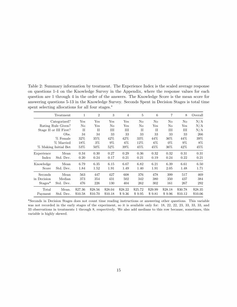
Table 2: Summary information by treatment. The Experience Index is the scaled average responseon questions 1-4 on the Knowledge Survey in the Appendix, where the response values for eachquestion are 1 through 4 in the order of the answers. The Knowledge Score is the mean score foranswering questions 5-13 in the Knowledge Survey. Seconds Spent in Decision Stages is total timespent selecting allocations for all four stages.∗

Treatment 1 2 3 4 5 6 7 8 Overall

Categorized? Yes Yes Yes Yes No No No No N/ARating Rule Given? No Yes No Yes No Yes No Yes N/A

Stage II or III First? II II III III II II III III N/AObs. 34 34 33 33 33 33 33 33 266

% Female 32% 35% 42% 42% 33% 44% 36% 44% 39%% Married 18% 3% 9% 6% 12% 6% 0% 9% 8%

% Making Initial Bet 53% 50% 52% 39% 45% 45% 36% 42% 45%

Experience Mean 0.34 0.30 0.27 0.29 0.36 0.32 0.32 0.31 0.31Index Std. Dev. 0.20 0.24 0.17 0.21 0.21 0.19 0.24 0.22 0.21

Knowledge Mean 6.79 6.35 6.15 6.67 6.82 6.21 6.39 6.61 6.50Score Std. Dev. 1.84 1.52 1.91 1.49 1.40 1.91 2.05 1.48 1.71

Seconds Mean 563 447 427 608 376 478 399 517 469in Decision Median 373 354 431 502 342 380 350 437 384

Stages* Std. Dev. 476 226 130 404 262 302 161 267 292

Total Mean. $27.36 $28.56 $28.04 $28.22 $25.72 $29.99 $28.18 $30.78 $28.35Payment Std. Dev. $10.58 $10.70 $10.18 $ 9.36 $ 9.95 $ 9.81 $ 9.96 $10.12 $10.06

*Seconds in Decision Stages does not count time reading instructions or answering other questions. This variablewas not recorded in the early stages of the experiment, so it is available only for: 18, 22, 22, 23, 33, 33, 33, and33 observations in treatments 1 through 8, respectively. We also add medians to this row because, sometimes, thisvariable is highly skewed.

15

Women in the study were significantly likelier to take the initial bet (55% vs 39% for men,

p-value less than 0.01) and had a significantly lower average knowledge score (5.91 vs 6.86) and

experience (0.22 vs 0.38). Both differences were significant with a p-value less than 0.0001.14

3.2 Investment in Trial 1

The first question is how subjects performed on the basic allocation task in Trial 1, without treat-

ments. The answer is that subjects invested most heavily in A and B, mostly avoided the dominated

assets, and did not naively diversify.

Figure 4 is a violin plot depicting the density function across subjects for investment in Trial

1, for each asset and cash. The median level of investment is represented in each plot by a white

dot, the interquartile range by a heavy black line, and the contours of the enveloping curve depict a

kernel density, effectively a rotated histogram. A and B were the only assets for which a significant

percentage of subjects invested $4 or more, and the mean investment in the two assets combined

was $7.91. For each of the domninated assets C, F, and Cash, 75% or more of subjects invested 0.

Investments in Asset D constituted the bulk of investment in the high-risk group of assets.

We can also ask to what extent subjects diversify, even though there is no value to investing in

more than two assets. Figure 5 depicts a violin plot for the cumulative investment across 6 assets

in Trial 1, with investments for each subject sorted in order of the amount invested. The figure

shows that the median investor has the bulk of their cash — almost $10 — invested in two or fewer

assets and all of their $12 invested in three or fewer assets. 75% of investors have at least $10 in

three or fewer assets. A small fraction of investors invests $12 across 6 assets and eleven subjects

at some point invested in 7 assets.15 The figure demonstrates that there is heterogeneity across

subjects, but also reinforces the conclusion that the bulk of investors do not naively diversify.

Finally, we checked for spurious correlation between subject behavior and treatments by comput-

ing the significance of the correlation between Trial 1 investments and each of the three treatments,

none of which are in effect in Trial 1. None of the correlations were significant at the 5% level.16

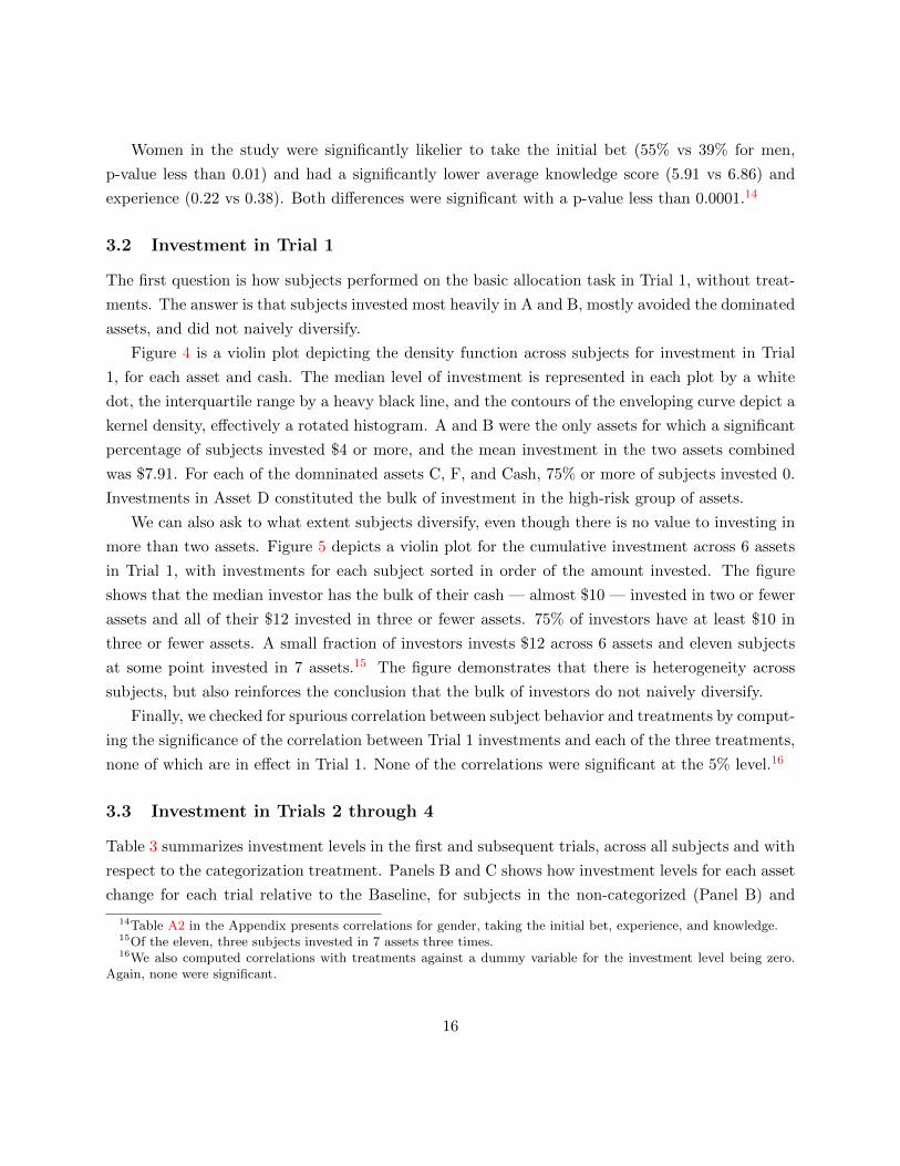
3.3 Investment in Trials 2 through 4

Table 3 summarizes investment levels in the first and subsequent trials, across all subjects and with

respect to the categorization treatment. Panels B and C shows how investment levels for each asset

change for each trial relative to the Baseline, for subjects in the non-categorized (Panel B) and

14Table A2 in the Appendix presents correlations for gender, taking the initial bet, experience, and knowledge.15Of the eleven, three subjects invested in 7 assets three times.16We also computed correlations with treatments against a dummy variable for the investment level being zero.

Again, none were significant.

16

●●●●●●●●●●●●●●●●●●●●●●●●●●●●●

●

●

●

●

●●

●

●

●

●●

●●

●●

●

●●

●●

●

●●●●

●

●

●

●

●●

●

●

●

●

●●

●●

●●

●

●●

●●●●●●●●

●

●●●

●

●●

●

●●

●

●

●

●●●●

●●

●●●●●●

●

●●●

●

●

●

●●

●

●

●

●●

●

●

●

●●

●

●

●

●

●

●

●

●

●

●●

●

●

●

●●

●

●●●

●

●●●

●

●●

●

●

●●

●

●●

●

●

●

●●

●

●

●

●

●

●

●

●●

●

●

●

●●

●

●

●●●

●

●

●

●●

●

●

●

●

●

●

●

●

●

●

●

●●

●

●●

●

●

●●

●

●

●

●

●

●

●

●

●

●

●

●

● ● ●0

2

4

6

8

10

12

A B C D E F Cash

Asset

Inve

stm

ent

Figure 4: Violin plot depicting investment by asset in Trial 1. The dark line in the center showsthe interquartile range, with the median a white dot. Black points indicate outliers. The overallshape is a kernel density plot.

17

●●●

●●●●

●●●

●

●

●

●●

●●

●

●

●

●●

●

●

●

●

●

●

●

●●

●

●

●●

●●

●

●

●●●

●

●

●

●

●

●●

●

●●●

●

●●

●●

●

●

●

●●●●

●●

●

●

●●

●●

●●●●●

●●●

●●●●●●●●

●

●●●●●●

●

●

● ● ● ●

0

2

4

6

8

10

12

1 2 3 4 5 6

Number of Assets

Cum

ulat

ive

Inve

stm

ent

Figure 5: Violin plot depicting the distribution of the number and quantity of assets held byinvestors in Trial 1. For a given subject, holdings are sorted from greatest to least and cumulated.The plot shows the number of dollars invested in the largest holding, the largest two holdings, etc.

18

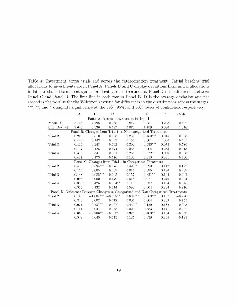
Table 3: Investment across trials and across the categorization treatment. Initial baseline trialallocations to investments are in Panel A. Panels B and C display deviations from initial allocationsin later trials, in the non-categorized and categorized treatments. Panel D is the difference betweenPanel C and Panel B. The first line in each row in Panel B -D is the average deviation and thesecond is the p-value for the Wilcoxon statistic for differences in the distributions across the stages.∗∗∗, ∗∗, and ∗ designate significance at the 99%, 95%, and 90% levels of confidence, respectively.

A B C D E F Cash

Panel A: Average Investment in Trial 1

Mean ($) 3.125 4.798 0.388 1.817 0.951 0.228 0.692Std. Dev. ($) 2.648 3.336 0.797 2.078 1.759 0.666 1.818

Panel B: Changes from Trial 1 in Non-categorized Treatment

Trial 2 0.225 0.310 0.093 −0.256 −0.450∗∗∗ −0.016 0.0930.446 0.143 0.297 0.155 0.001 1.000 0.425

Trial 3 0.426 −0.248 0.062 −0.302 −0.450∗∗∗ −0.078 0.5890.117 0.125 0.474 0.036 0.004 0.283 0.015

Trial 4 0.310 0.341 −0.031 −0.256 −0.372∗∗ 0.000 0.0080.427 0.173 0.676 0.180 0.018 0.331 0.430

Panel C: Changes from Trial 1 in Categorized Treatment

Trial 2 0.418 −0.694∗∗∗ −0.075 0.425∗∗ −0.090 0.142 −0.1270.154 0.005 0.169 0.015 0.695 0.136 0.239

Trial 3 0.448 −0.985∗∗∗ −0.045 0.157 −0.321∗∗ 0.104 0.6420.095 0.000 0.479 0.515 0.027 0.240 0.294

Trial 4 0.373 −0.425 −0.164∗∗ 0.119 0.037 0.104 −0.0450.336 0.132 0.014 0.592 0.604 0.234 0.270

Panel D: Difference Between Changes in Categorized and Non-Categorized Treatments

Trial 2 0.193 −1.004∗∗∗ −0.168∗∗ 0.681∗∗∗ 0.360∗∗∗ 0.157 −0.2200.829 0.002 0.012 0.006 0.004 0.309 0.755

Trial 3 0.021 −0.737∗∗ −0.107∗ 0.459∗∗ 0.129 0.182 0.0530.741 0.041 0.055 0.029 0.583 0.141 0.232

Trial 4 0.063 −0.766∗∗ −0.133∗ 0.375 0.409∗∗ 0.104 −0.0530.942 0.049 0.073 0.125 0.038 0.205 0.121

19

categorized treatment (Panel C). Panel D shows the difference in these changes between the two

treatments (i.e., it is a difference in differences).

The main result, in Panel D, is that the change in investment is consistent with the rating

change due to categorization. Subjects invest more when the rating is higher (D and E), less when

it is lower (B and C), and there is no change when the rating is the same across treatments (A and

F). Specifically:

• Panel A shows that average investment is greatest in assets A and B ($7.91 combined in

Trial 1) and lowest in the dominated assets, C and F ($0.62 combined in Trial 1). Average

investment in Cash in Trial 1 was $0.69.

• Panel B shows that, in non-categorized treatments, ratings in Trials 2 and 3 have little effect

on investment levels. The exception is E, which receives one star in the non-categorized

treatments, and for which investment falls significantly. This drop remains when ratings are

removed in Trial 4.

• Panel C shows that categorization reduces investment in B in both Trials 2 and 3, and to a

lesser extent increases investment in D. This pattern is consistent with the categorized star

ratings of B (2 stars) and D (3 stars).

• Panel D shows no categorization/rating interaction effects for A (always rated 3 stars) and

F (always rated 1 star). But, in Stage 2, investment levels in B and C are both significantly

lower when they are rated lower due to categorization. Similarly, investment levels in D and

E are significantly higher when they are rated higher due to categorization. This is exactly

the effect we hypothesize. The effects on B and C remain when subjects self-rate and when

ratings are removed. The effect for D remains when subjects self-rate and for E when ratings

are removed.

• Consistent with Figure 5, subjects do not naively diversify: a test for equality of investment

across investments A through F is rejected.17 Subjects do not use the 1/N rule (Benartzi and

Thaler, 2001).

The results in Table 3 are inconsistent with both the experimenter demand effect and the notion

that subject responses are due to cognitive challenges. There is no significant change from Trial

1 to Trial 2 in investment in A, or in B in the non-categorized treatment; this rules out subjects

naively investing in accord with stars. The fact that subjects do reduce investment in B when it

17A Kruskal-Wallis test rejects equality of means with a p-value of 2.2e-16.

20

is rated two stars suggests that the two star rating is a reduction from the implicit rating they

assigned in Trial 1. We cannot definitively say why subjects reduce investment in B, but cognitive

dissonance seems like a possible explanation.

3.4 Cash Holdings

As a consistency check, we examine investment in cash, for which positive holdings are never

optimal. Across the 4 trials, 162 subjects never hold cash. An additional 39 subjects have average

cash holdings of less than $1 per trial.18 Thus, 80% of the subjects essentially hold no cash. At

the other extreme, one subject in the categorized group holds only cash throughout the experiment

and one subject exclusively holds cash in two trial. The remaining subjects who hold cash at some

point do so only once.19 Cash-holding peaks in Trial 3, when subjects are asked to provide ratings.

Eighteen subjects in this case invest only in cash, with 14 of those in the treatment that did not

explain the rating rule. We have no definitive explanation for this behavior, but it seems likely that

asking subjects to actively engage in analysis created poorer outcomes for a significant subset.20

We conclude that the vast majority of subjects understand the suboptimality of cash. It is

most extensively used when subjects have to assign ratings, which presumably creates a significant

cognitive load.

3.5 Regression Analysis of Investment in All Trials

We now use regression to examine investment behavior in more detail. We want to see how subject

characteristics affect performance and whether subject knowledge mediates treatment effects. For

each asset, we run a regression across all trials controlling for subject characteristics and treatments:

Iijk = αi + β1Xj + β2Tk=2X2,j + β3Tk=3X3,j + β4Tk=4X4,j + εi,j (1)

where Xj is a vector of subject characteristics and Xk,j is a vector of controls specific to each

trial. Tk=n is a dummy variable that takes the value 1 in Trial n. We estimate a censored regres-

18Table A3 shows cash holdings broken down by trial and whether the subject was in the group that was told therating rule.

19A probit regression shows that having a higher knowledge score makes it less likely that subjects will invest solelyin cash. Other characteristics are not predictive.

20Subjects responded to a satisfaction survey after each trial and were asked if they wished they could changetheir decision. None of the 18 subjects investing only in cash in the Self-Rated trial said they wished they couldchange their decision, and for the 10 who did wish they could change, none invested anything in cash. Ten of the 18experienced self-rating first, and eight of those were in the treatment not providing the rating rule.

21

sion to account for investment amounts being between 0 and 12.21 We calculate robust standard

errors, clustered by subject. Because there is effectively no treatment in Trial 1, we control for

subject characteristics and, as a placebo, categorization. In trials 2-4, results depend both upon

characteristics and treatments. Equation (1) should be viewed as an elaboration upon Table 3.

To summarize the main results, we find that more knowledgable and experienced subjects behave

more rationally in the baseline trial and that taking the initial bet is associated with holding riskier

investments. In later trials, subjects are affected by the categorization treatment, they invest in

accord with the ratings they assign, and knowledge and experience do not significantly mitigate

the effect of treatments.

Explanatory variables, for which summary statistics are provided in Table 4, include:

Knowledge Total correct answers for the nine questions on the knowledge test, normalized to be

between 0 and 1, less the mean across all subjects.

Experience Experience index, normalized to be between 0 and 1, less the mean across all subjects.

Gender Dummy variable, female equals one.

RiskBet Dummy variable for taking the initial bet.

Cat Dummy variable for the treatment with categorization.

Rule Dummy variable for the treatment in which the subject is told the rating rule.

SelfRank Rating assigned by the subject in the third trial for a given asset, less the uncategorized

rating (Panel B in Figure 1).

Note that we have a choice in equation (1) about specifying subject characteristics. We can

either allow their effect to vary individually in each trial or include them in the regression without

conditioning on the individual trials. We include them without conditioning, so they are interpreted

as providing the baseline across all trials. In some cases we interact characteristics with treatment

dummies to see if knowledge (for example) alters the effect of the treatment. We discuss trial-

specific effects of characteristics where relevant.

We present results separately pertaining to each trial rather than presenting the entire regression

in one table. Two points relating to statistical significance are worth noting. First, because of the

large number of coefficients in the regressions, we expect to see some significant coefficients at lesser

21Investments range from $0 to $12 and are discrete, occurring in one dollar increments. As a robustness check, wealso estimated ordered probit models and got essentially identical results. We present the censored regression modelsbecause they are easier to interpret.

22

Table 4: Summary statistics for regression variables. “Female” is a dummy variable where malesare 0, females are 1; “Experience” and “Knowledge” are both based on a survey response scaledfrom 0 to 1 and normalized to have mean 0; “RiskBet” is a dummy variable for taking the initialrisky bet; “Cat” and “Rule” are dummy variables for being in the treatments that are categorizedand told the rating rule; and “Selfrank A - F” are the stars assigned by subjects minus the numberof stars those assets have in the non-categorized treatment.

Mean Std Dev Min Max

Female 0.384 0.487 0.000 1.000Experience 0.000 0.210 -0.315 0.685Knowledge -0.000 0.190 -0.722 0.278

RiskBet 0.456 0.498 0.000 1.000Cat 0.510 0.500 0.000 1.000

Rule 0.494 0.500 0.000 1.000Selfrank A -0.365 0.638 -2.000 0.000Selfrank B -0.430 0.560 -2.000 0.000Selfrank C -0.452 0.633 -1.000 1.000Selfrank D 0.407 0.621 -1.000 1.000Selfrank E 0.650 0.551 0.000 2.000Selfrank F 0.190 0.560 0.000 2.000

significance levels as a result of random variation. We try not to over-interpret these cases. Second,

across trials, more than 75% of subjects invest zero in assets C and F. Asset E also has significant

zero investment. This is rational, but it means that the regression coefficients in those cases load

on the small number of subjects who do invest. Idiosyncratic behavior may be overweighted. We

report results for all assets, but focus our attention on A, B, and D.

3.5.1 Effects of Subject Characteristics in Trial 1

Table 5 presents those regression coefficients in equation (1) which are not multiplied by a dummy

for Trials 2 through 4.22 These coefficients are thus approximately the unconditional effect of

characteristics, with one placebo variable, a dummy for the effect of categorization in Trial 1. The

coefficients in all cases are computed conditional on the observation not being censored.

Table 5 shows that subjects responded to the economic characteristics of the investments, and

departed in ways consistent with the personal characteristics including knowledge and experience.

Investments A, B, and D have significant positive intercepts. The other assets have significant

negative intercepts. The censored regression allows the independent variables to explain the non-

22Subject characteristics are effectively repeated for each trial, so there are only 266 observations on each charac-teristic as opposed to 1052 observations. Clustered standard errors correct for this repetition. The alternative of afixed effect model cannot be used because each subject only participates in one treatment.

23

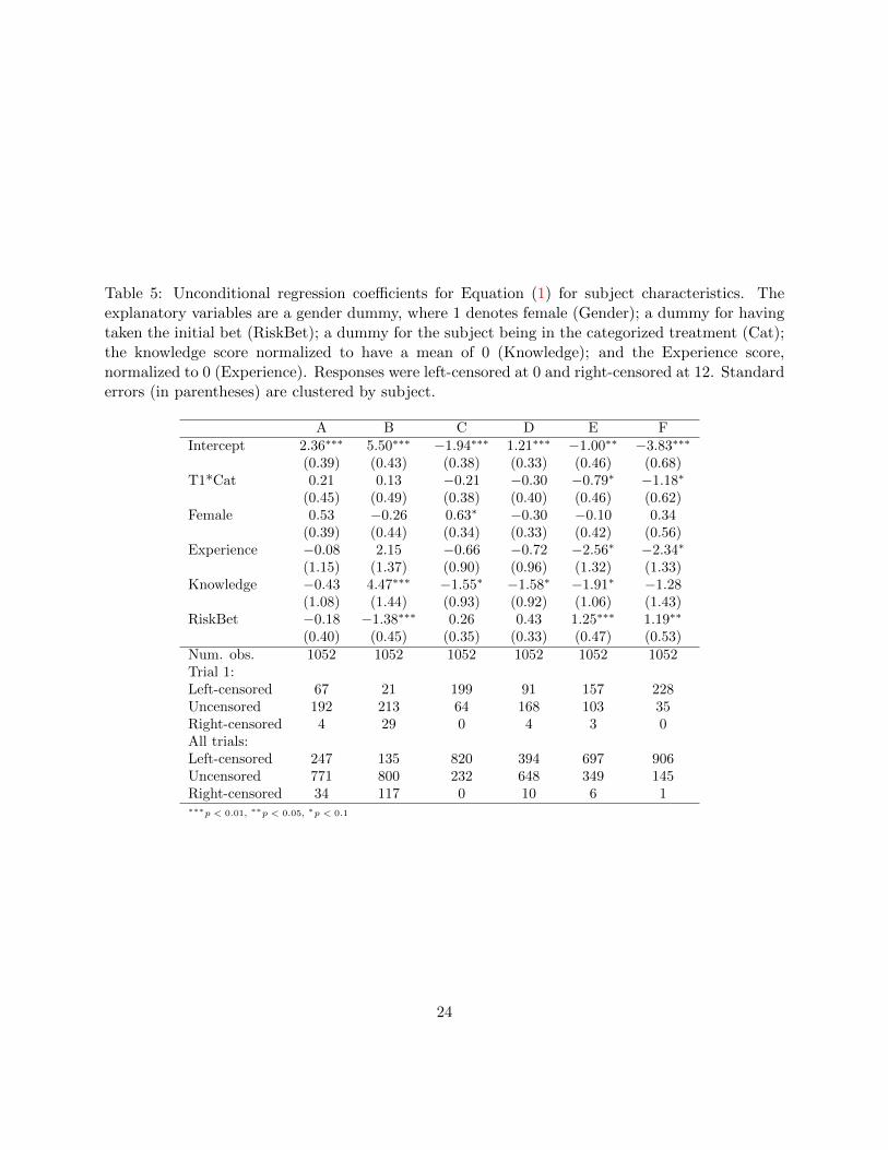
Table 5: Unconditional regression coefficients for Equation (1) for subject characteristics. Theexplanatory variables are a gender dummy, where 1 denotes female (Gender); a dummy for havingtaken the initial bet (RiskBet); a dummy for the subject being in the categorized treatment (Cat);the knowledge score normalized to have a mean of 0 (Knowledge); and the Experience score,normalized to 0 (Experience). Responses were left-censored at 0 and right-censored at 12. Standarderrors (in parentheses) are clustered by subject.

A B C D E FIntercept 2.36∗∗∗ 5.50∗∗∗ −1.94∗∗∗ 1.21∗∗∗ −1.00∗∗ −3.83∗∗∗

(0.39) (0.43) (0.38) (0.33) (0.46) (0.68)T1*Cat 0.21 0.13 −0.21 −0.30 −0.79∗ −1.18∗

(0.45) (0.49) (0.38) (0.40) (0.46) (0.62)Female 0.53 −0.26 0.63∗ −0.30 −0.10 0.34

(0.39) (0.44) (0.34) (0.33) (0.42) (0.56)Experience −0.08 2.15 −0.66 −0.72 −2.56∗ −2.34∗

(1.15) (1.37) (0.90) (0.96) (1.32) (1.33)Knowledge −0.43 4.47∗∗∗ −1.55∗ −1.58∗ −1.91∗ −1.28

(1.08) (1.44) (0.93) (0.92) (1.06) (1.43)RiskBet −0.18 −1.38∗∗∗ 0.26 0.43 1.25∗∗∗ 1.19∗∗

(0.40) (0.45) (0.35) (0.33) (0.47) (0.53)Num. obs. 1052 1052 1052 1052 1052 1052Trial 1:Left-censored 67 21 199 91 157 228Uncensored 192 213 64 168 103 35Right-censored 4 29 0 4 3 0All trials:Left-censored 247 135 820 394 697 906Uncensored 771 800 232 648 349 145Right-censored 34 117 0 10 6 1∗∗∗p < 0.01, ∗∗p < 0.05, ∗p < 0.1

24

censored variation in subject holdings.23 Subjects who took the initial bet invested $1.22 more in

the highest risk asset, E, more in F, and $1.25 less in asset B. A higher knowledge score is associated

with increased investment in B and reduced investment in C, E, and F. Specifically, one additional

correct question on the knowledge test was associated with a $0.50 (= 4.47/9) increased investment

in B. For all but asset A, knowledge and the risky bet had offsetting signs.24 Finally, subjects with

more investment experience invested less in E and F. The coefficient can be interpreted as the effect

of going from no experience to maximum experience.

Women invested more in C, but otherwise, gender effects were not evident. As a placebo test, we

included a dummy for the subject being in the categorized treatment. This dummy has significance

at the 10% level for E and F.

3.6 The Effect of Star Ratings in Trials 2 and 3

The second and third trials exposed subjects to star ratings. Two aspects of these trials are

especially important. First, in Trial 2, where subjects are shown ratings, the question is whether

knowledge mediates the effect shown in Table 3. Second, in Trial 3, in which subjects assign star

ratings to the investments, we impose the constraint that they assign equal numbers of one, two,

and three star ratings, either within categories or not, depending on the treatment. The question

is whether this active participation affects investment decisions.

3.6.1 Trial 2

Table 6 shows the coefficients from regression equation 1 for the trial in which subjects are given

ratings, with half of the subjects told how the assets are rated. There are three important results

in the table.

First, categorization affects investment decisions. Subjects exposed to categorization reduce

investment in assets B and C — both of which have one less star when categorized — by over $1

each. To interpret this finding, recall from Table 3 that initial investment was greatest for B, A,

and D, in that order, with average investment less than $1 for C, E, and F. We would expect an

effect in B if anywhere, and the $1 decline in B is economically significant. There is no comparable

effect for A and F, for which the rating is not affected by categorization. There is also no effect on

D, for which the rating is increased by categorization.

23Because the regressions are censored, coefficients need not sum to zero across the assets, and the intercepts donot sum to 12 as they would with simple OLS.

24We also estimated this regression using question 7, queston 13, and the sum from the remaining knowledge scorequestions. Those correctly calculating the return in question 7 invested more in asset B and less in assets D andCash. A higher score on the remaining knowledge questions were associated with more investment in B and less inC and Cash.

25

Second, financial knowledge does not alter the effect of the categorization treatment. Knowledge

is interacted with the Trial 2 dummy individually and interacted with the category and rating

rule treatment dummies. While more knowledgeable investors in the first trial invest more in B,

knowledge does not mediate the effect of categorization. This remains true when performing F-tests

on sums of coefficients.25,26

Third, there is no strong effect associated with subjects being told the rating rule. The only

significant effect, with an F-test taking account of all interactions, occurs with Asset C; being given

the rating rule leads to $1 less investment for subjects with one additional knowledge score point

in the uncategorized treatment (t-statistic of -1.88), and $2.53 less in the categorized treatment

(t-statistic of -3.45).

Finally, the Trial 2 dummy variable is insignificant for all but asset E. As in our discussion of

Table 3, we view this as inconsistent with the experimenter demand effect and with cognitively-

challenged subjects using ratings to help make decisions.

3.6.2 Trial 3

Subjects are asked to provide their own ratings while choosing investment amounts. This raises

two questions:

1. Did subjects assign reasonable ratings?

2. Did subjects invest in accord with the ratings they assigned?

If subjects invest in accord with their ratings, then we should generally see higher ratings

correspond with more investment. Subjects in the categorized treatment, however, may be forced

to assign a rating which conflicts with their investment (rating B at 2 stars). We find that self-

assigned ratings are strongly associated with investment behavior, except when we force a conflict.

Forcing a low rating, in other words, does not affect the investment.

Because most investment is in A and B, we initially focus the discussion on those assets.

Subject ratings Subjects assign ratings that generally correspond with those in Table 1, but

which also are affected by treatments in an unsurprising way.27 For example, subjects consistently

25Regressions using the individual knowledge score components, not reported, show subjects displaying computationability investing more in B and less in E, F, and cash, but importantly, knowledge still does not mitigate the effectsof categorization.

26A chi-squared test showed no additional explanatory power from adding a dummy for the rating rule interactedwith categorization and knowledge.

27Table A4 in the Appendix shows the percentage of subjects assigning each rating in each of four treatments(categorization by the rank rule).

26

Table 6: Regression coefficients for Equation (1) pertaining to Trial 2, denoted by the dummyvariable T2. The intercept from Table 5 is duplicated for reference. The explanatory variables fortrial 2 are a dummy for being in the categorization treatment (Cat); a dummy for being in thetreatment where the rating rule is provided (Rule); and the knowledge score normalized to havea mean of 0 (Knowledge). Responses were left-censored at 0 and right-censored at 12. Standarderrors (in parentheses) are clustered by subject.

A B C D E FIntercept 2.36∗∗∗ 5.50∗∗∗ −1.94∗∗∗ 1.21∗∗∗ −1.00∗∗ −3.83∗∗∗

(0.39) (0.43) (0.38) (0.33) (0.46) (0.68)T2 0.22 0.36 0.51 −0.49 −1.39∗∗∗ −0.02

(0.35) (0.38) (0.32) (0.34) (0.47) (0.44)T2*Cat 0.62 −1.09∗∗ −1.21∗∗∗ 0.63 0.28 −0.48

(0.46) (0.55) (0.44) (0.39) (0.47) (0.63)T2*Rule 0.05 −0.04 −0.64 0.08 0.40 −0.40

(0.46) (0.54) (0.45) (0.39) (0.49) (0.63)T2*Cat*Knowledge 2.92 −0.75 −2.57 −3.26∗∗ 0.91 −2.24

(2.09) (2.31) (1.79) (1.59) (1.68) (2.80)T2*Rule*Knowledge −0.73 −0.72 −3.41∗ 0.93 2.44 −3.41

(1.95) (2.12) (1.79) (1.60) (1.92) (2.51)Num. Obs. (trial) 263 263 263 263 263 263Left-censored 56 30 205 98 176 225Uncensored 200 202 58 163 86 38Right-censored 7 31 0 2 1 0∗∗∗p < 0.01, ∗∗p < 0.05, ∗p < 0.1

27

rated A highly except in the categorized treatment when not told the rule used to construct the

ratings. In this case they roughly split 50-50 between giving the top rating to A and B.28 As

expected, categorization reduces the correspondence between subject-assigned rating and the ob-

jective rating. Overall, when given the rating rule, between 80% and 90% of subjects ranked the

assets in accord with the rule based on the ratio of return to risk.29

Table 7 reports the results of a regression analysis of the self-ratings. The table shows that

categorization has a large effect on ratings, reducing the ratings assigned to B and C and increasing

the rating assigned to D and E. Categorization also reduced the rating for A, presumably because

subjects wished to rate B more highly. Knowing the rating rule has a small effect; non-categorized

subjects told the rating rule, for example, gave a higher rating to C and a lower rating to E, in

accord with their Sharpe ratio. Knowledge and experience, however, do not affect the self-rating.

On the whole, subjects rate investments reasonably, subject to the restrictions we impose. It is

interesting to note that RiskBet and knowledge have no effect on how subjects do the ranking, but

as shown in Table 5 these variables do affect investment behavior.

Effect of subject ratings on investment Table 8 reports the Trial 3 coefficients from regression

equation 1. The new explanatory variable is SelfRank, which is defined as the difference between

the rating assigned by the subject and the non-categorized rating. For example, Asset B has a non-

categorized rating of 3, so the self-rating is 0 if the subject assigns B the non-categorized rating of

3 stars, and -1 if a subject assigns it two stars. SelfRank is included as a standalone variable, and

interacted with the categorization and rule dummies. The standalone coefficient in the regression

shows that subjects not in the categorized treatment (i.e., for whom Cat = 0) invest more in assets

to which they assign higher ratings. The magnitude is between $1.25 and $4.31 per assigned star.

What happens when categorized subjects are encouraged to give two stars to both B and E?

For both assets, the regression shows that the net effect of the self-ranking variable for categorized

subjects is zero (for B) or negative (for E). A subject forced to rate B two stars has a zero net effect

of the ranking (the coefficients on the self-rating, and rating/categorization interaction dummy sum

to almost exactly zero). For E, a categorized subject not told the ranking rule has a negative effect

of the forced higher ranking. It is unforced star ratings that affect investment. Being told the rank

rule does not affect this result for most assets. It does seem to matter for E, offsetting the effect

of the rating. It is worth noting that Asset E suffers from the small sample problem with only

28Panel A also implicitly suggests that some subjects were confused about ranks, and gave A a 1 and C a 3.29As another way to assess subject ratings, we can compute correlations between subject and “correct” ratings

across different treatments. The correlation was 0.82 for the uncategorized and 0.67 for the categorized treatment,and 0.71 without the rating rule and 0.78 with the rating rule. The lowest correlation was 0.65 in the categorizedtreatment without the rating rule, and the highest was 0.87 in the uncategorized treatment with the rating rule.

28

Table 7: OLS regressions explaining subject-assigned rank in Trial 3. The dependent variable isthe subject-assigned rank. The explanatory variables are a gender dummy, where 1 denotes female(Female); a dummy for having taken the initial bet (RiskBet); a dummy for the subject being inthe categorized treatment (Cat); a dummy for the subject receiving the rating rule (Rule), andvariables denoting the knowledge score normalized to zero (Knowledge) and the experience scorenormalized to zero (Experience). Standard errors are in parentheses.

A B C D E FIntercept 2.78∗∗∗ 2.89∗∗∗ 1.63∗∗∗ 2.16∗∗∗ 1.43∗∗∗ 1.12∗∗∗

(0.11) (0.08) (0.10) (0.10) (0.08) (0.10)Female −0.08 0.02 0.02 −0.03 −0.02 0.09

(0.08) (0.06) (0.08) (0.07) (0.06) (0.08)Experience 0.07 0.19 0.00 −0.02 −0.07 −0.18

(0.20) (0.15) (0.19) (0.17) (0.15) (0.19)RiskBet −0.06 −0.13∗∗ 0.16∗∗ −0.13∗∗ 0.07 0.09

(0.08) (0.06) (0.07) (0.06) (0.05) (0.07)Cat −0.44∗∗∗ −0.46∗∗∗ −0.45∗∗∗ 0.75∗∗∗ 0.53∗∗∗ 0.07

(0.10) (0.08) (0.10) (0.09) (0.07) (0.10)Rule 0.15 −0.01 0.23∗∗ −0.10 −0.26∗∗∗ −0.01

(0.11) (0.08) (0.10) (0.09) (0.08) (0.10)Knowledge 0.07 0.07 0.40 −0.07 −0.21 −0.26

(0.36) (0.26) (0.33) (0.30) (0.25) (0.33)Cat*Rule 0.21 −0.35∗∗∗ −0.22 −0.04 0.30∗∗∗ 0.10

(0.15) (0.11) (0.14) (0.12) (0.11) (0.14)Cat*Knowledge 0.09 0.14 −0.83∗∗ 0.35 0.62∗∗ −0.36

(0.39) (0.29) (0.36) (0.33) (0.28) (0.36)RiskBet*Knowledge 0.49 −0.11 −0.60 0.24 −0.20 0.17

(0.40) (0.30) (0.37) (0.34) (0.29) (0.37)R2 0.15 0.41 0.27 0.37 0.43 0.07Adj. R2 0.12 0.39 0.24 0.35 0.41 0.04Num. obs. 263 263 263 263 263 263RMSE 0.60 0.44 0.55 0.50 0.43 0.55∗∗∗p < 0.01, ∗∗p < 0.05, ∗p < 0.1

29

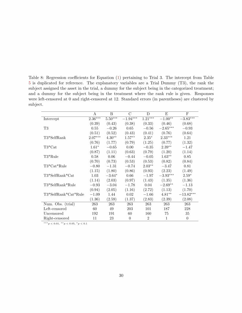
Table 8: Regression coefficients for Equation (1) pertaining to Trial 3. The intercept from Table5 is duplicated for reference. The explanatory variables are a Trial Dummy (T3), the rank thesubject assigned the asset in the trial, a dummy for the subject being in the categorized treatment;and a dummy for the subject being in the treatment where the rank rule is given. Responseswere left-censored at 0 and right-censored at 12. Standard errors (in parentheses) are clustered bysubject.

A B C D E FIntercept 2.36∗∗∗ 5.50∗∗∗ −1.94∗∗∗ 1.21∗∗∗ −1.00∗∗ −3.83∗∗∗

(0.39) (0.43) (0.38) (0.33) (0.46) (0.68)T3 0.55 −0.26 0.65 −0.56 −2.65∗∗∗ −0.93

(0.51) (0.52) (0.43) (0.41) (0.76) (0.64)T3*SelfRank 2.07∗∗∗ 4.30∗∗ 1.57∗∗ 2.35∗ 2.33∗∗∗ 1.21

(0.76) (1.77) (0.79) (1.25) (0.77) (1.32)T3*Cat 1.61∗ −0.65 0.00 −0.35 2.39∗∗ −1.47

(0.87) (1.11) (0.63) (0.79) (1.20) (1.14)T3*Rule 0.58 0.06 −0.44 −0.05 1.63∗∗ 0.85

(0.70) (0.73) (0.53) (0.53) (0.82) (0.84)T3*Cat*Rule −0.80 −1.31 −0.74 2.03∗∗ −3.47 0.81

(1.15) (1.80) (0.86) (0.93) (2.23) (1.49)T3*SelfRank*Cat 1.03 −3.64∗ 0.66 −1.97 −3.93∗∗∗ 2.59∗

(1.14) (2.03) (0.97) (1.43) (1.35) (1.36)T3*SelfRank*Rule −0.93 −3.04 −1.78 0.04 −2.69∗∗ −1.13

(0.94) (2.05) (1.16) (2.72) (1.13) (1.70)T3*SelfRank*Cat*Rule −1.09 1.44 0.02 −1.66 4.81∗∗ −13.82∗∗∗

(1.36) (2.59) (1.37) (2.83) (2.39) (2.08)Num. Obs. (trial) 263 263 263 263 263 263Left-censored 60 49 203 101 187 228Uncensored 192 191 60 160 75 35Right-censored 11 23 0 2 1 0∗∗∗p < 0.01, ∗∗p < 0.05, ∗p < 0.1

30

75 uncensored subjects. Otherwise, there is little evidence that being told the rating rule has any

effect on investment.30

3.6.3 Trial 4

Table 9 reports the coefficients from regression equation 1 for the final trial, which is an untreated

repeat of the first. As such, the Trial 4 regression variables measure the effects from subjects having

participated in the previous trials. The results are generally not significant. There is a secular

decline in investment in D and E, and more knowledgeable investors sharply reduce investment in

F. The coefficients on categorization for B and C are similar to but attenuated from Trial 2 (Table

6), with only that on C being statistically significant. This is consitent with the result from Table

3 that categorized investors invested less in B and C than non-categorized investors in Trials 2-4,

and for D and E the same effect was zero or positive, in line with the star rating shifts due to

categorization.

3.7 Overall Investment Performance

The primary focus of the preceding analysis has been on investment in individual assets. Table

10 examines overall portfolio performance as measured by the portfolio Sharpe ratio. The analysis

confirms that categorization harms performance. The table presents regressions explaining the

Sharpe ratio and its components in Trial 1, and the difference between the Sharpe ratio in later

trials and that in Trial 1.

In Trial 1, more knowledgable investors have a higher expected return and no greater risk, for a

higher Sharpe ratio. Those who take the initial bet assume greater risk and an insignificantly lower

expected return, which reduces their Sharpe ratio. Gender and experience do not affect overall

performance.

In Trial 2, in line with the results in Table 3, categorization reduces performance. More knowl-

edgable subjects are less harmed by categorization, but knowledge overall is statistically insignifi-

cant (p-value of 0.138 in an F-test).

The only other statistically significant effect is that those who took the initial bet recoup their

performance somewhat in Trials 2 and 4; this may be due to the secular decline in holdings of Asset

E evident in Table 3. Interestingly, performance is not recouped in Trial 3.

30In Table 8, note the large negative coefficient for SelfRank for Asset F, for subjects in the categorized treatmentwho are told the rank rule. Nine subjects gave asset F a rank of three stars and invested 0, instead investing primarilyin A, B, and D. These same subjects ranked B and D low, but invested heavily in them. One possible explanation isthat these subjects misunderstood the star rating, and the regression coefficient is the result of the regression tryingto fit this behavior.

31

Table 9: Regression coefficients for Equation (1) pertaining to Trial 4. The intercept from Table 5is duplicated for reference. The explanatory variables are a Trial dummy (T4) and a dummy for thesubject being in the categorized treatment. Responses were left-censored at 0 and right-censoredat 12. Standard errors (in parentheses) are clustered by subject.

A B C D E FIntercept 2.36∗∗∗ 5.50∗∗∗ −1.94∗∗∗ 1.21∗∗∗ −1.00∗∗ −3.83∗∗∗

(0.39) (0.43) (0.38) (0.33) (0.46) (0.68)T4 0.60 0.00 −0.26 −0.62∗ −1.16∗∗ −0.47

(0.42) (0.45) (0.36) (0.35) (0.47) (0.50)T4*Cat 0.33 −0.86 −0.90∗∗ 0.22 0.23 −0.53

(0.51) (0.55) (0.42) (0.40) (0.48) (0.65)T4*Knowledge 0.46 0.87 −1.16 1.08 −1.07 −3.24∗∗

(1.36) (1.47) (0.92) (0.96) (1.18) (1.42)T4*Gender −0.55 0.48 0.38 0.41 0.17 0.89

(0.45) (0.47) (0.33) (0.35) (0.44) (0.55)T4*RiskBet −0.05 0.38 −0.13 0.02 −0.13 −0.35

(0.40) (0.44) (0.32) (0.33) (0.40) (0.50)T4*Experience −0.63 1.06 1.86∗∗ −0.43 −1.30 0.46

(1.17) (1.34) (0.84) (0.85) (1.03) (1.08)Num. Obs. (trial) 263 263 263 263 263 263Left-censored 64 35 213 104 177 225Uncensored 187 194 50 157 85 37Right-censored 12 34 0 2 1 1∗∗∗p < 0.01, ∗∗p < 0.05, ∗p < 0.1

32

Table 10: OLS regressions. For Trial 1 the dependent variables are the expected return, returnstandard deviation (one-half the range), and the Sharpe ratio (the expected return divided by thestandard deviation), for Trials 2 through 4, the dependent variable is the change in the Sharperatio from Trial 1. 1 and across trials 2 through 4. An average Sharpe ratio could not be computedfor the 22 subjects who in at least one trial invested $12 in cash.

Trial 1 Sharpe Ratio, Trials 2-4Exp Ret Std Dev Sharpe T2 - T1 T3 - T1 T4 - T1

Intercept 0.845∗∗∗ 0.788∗∗∗ 1.103∗∗∗ 0.038∗∗ 0.026 0.046∗∗

(0.009) (0.012) (0.013) (0.016) (0.018) (0.019)Female −0.024∗∗ −0.013 −0.016 0.018 0.006 −0.015

(0.012) (0.015) (0.016) (0.014) (0.016) (0.017)Experience 0.075∗∗ 0.024 0.051 −0.029 0.026 −0.018

(0.030) (0.039) (0.042) (0.037) (0.042) (0.043)Knowledge 0.243∗∗∗ 0.049 0.229∗∗∗ −0.037 −0.022 −0.008

(0.031) (0.040) (0.043) (0.062) (0.072) (0.075)RiskBet −0.018 0.078∗∗∗ −0.112∗∗∗ 0.011 0.033 0.053∗∗

(0.011) (0.014) (0.015) (0.018) (0.021) (0.022)Cat −0.051∗∗∗ −0.020 −0.035

(0.018) (0.021) (0.022)Rule −0.009 −0.001 −0.009

(0.013) (0.014) (0.015)RiskBet*Cat 0.035 −0.005 0.007

(0.026) (0.029) (0.030)Knowledge*Rule −0.000 0.042 −0.004

(0.069) (0.081) (0.084)Knowledge*Cat 0.119∗ 0.022 0.125

(0.070) (0.082) (0.084)

R2 0.131 0.037 0.125 0.024 0.010 0.025Adj. R2 0.127 0.033 0.121 0.014 −0.002 0.014Num. obs. 872 872 863 860 796 852RMSE 0.155 0.201 0.214 0.185 0.203 0.218

∗∗∗p < 0.01, ∗∗p < 0.05, ∗p < 0.1

33

4 Related Literature

This paper is related to several distinct areas of the behavioral literature. Our goal in this section is

to provide some overarching context and relate results in the literature to our findings. As discussed

in the introduction, we discuss the relation of our findings to work on presentation effects, the effects

of financial knowledge, cognitive limitations, and difficulties making portfolio decisions.

4.1 Presentation Effects

Subjects have full information about investments. Why would they respond to ratings? There

are at least two obvious possibilities. One is that subjects believe the ratings convey additional

information. In this case we would expect financial knowledge to mitigate the effect of categorized

ratings. There is no significant mitigation from knowledge. Further, we would expect that explain-

ing that ratings are based on the Return/Risk Ratio would mitigate the effect. To the degree that

rule interactions are significant in Trials 2 and 3, explaining that the rating rule seems to reinforce

the response to to ratings.

A second possibility is that experimental subjects may respond to star rating here because they

wish to please the experimenter, a response known as the experimenter demand effect (Zizzo, 2010).

In our experiment, this behavior has real consequences, as blind adherence to the rating lowers the

expected payoff in some treatments. The question of whether subjects follow guidance against their

financial interest, however, is precisely the point of this study. This mirrors the possibility that,

in practice, investors invest in accord with ratings (for example) simply because those ratings are

supplied by an advisor or a ratings firm. We conclude that ratings affect performance.

The response to ratings relates to the general question of how subjects respond to presentation

of information. An investor making an investment decision will examine advertisements, literature,

reports, and possibly data about investment products and strategies. There is evidence that pre-

sentation of this information, including ratings, affects investment decisions for reasons unrelated

to the economic characteristics of the investment.

Several papers look explicitly at the effects of ratings:

• Chen et al. (2014) examine split-rated bonds (i.e., those where rating agencies disagree about

the bond rating) for which a bond index redefinition changed their status as investment

grade. They show that bond yields changed in response to this purely mechanical redefinition.

Because there was no new information about the bond, this real-world experiment resembles

our assignment of stars, and, as with our experiment, finds real effects.

• In a related vein, Del Guercio and Tkac (2008) and Reuter and Zitzewitz (2015) examine

34

whether equity mutual fund flows respond to Morningstar rating changes. Del Guercio and

Tkac (2008) find that an increase in the star rating of a fund is accompanied by an inflow

of funds, even after controlling for historical return characteristics. Reuter and Zitzewitz

(2015), in a study of size and performance, also document a relationship between the rating

and flows. Our findings are broadly consistent with theirs, but the settings are different.

Because they use aggregate investment data, neither study can distinguish between existing

investors changing their holdings in response to a ratings change (the intensive margin) and

new investors attracted to a newly higher rating (the extensive margin). For the same reason,

neither can examine investor heterogeneity. Our study examines the intensive margin, exam-

ining subjects in a given treatment who either see star ratings or not, and then comparing

subjects across treatments. With both papers there is also the possibility that investors be-

lieve ratings convey real information about expected returns.31 In this regard, the findings in

Chen et al. (2014) are more purely about rating changes. Finally, responses to ratings changes

for a given fund does not address whether investors are misled by cross-category comparisons

of ratings.

• Our experiment is complementary to that in Bateman et al. (2016), who vary the presen-

tation of investment characteristics when asking subjects to rank portfolios. We leave the

presentation unchanged, but find effects nevertheless.

Other papers consider the number of funds offered as an element of presentation.

• Benartzi and Thaler (2001) posit that investors choosing funds in a retirement account naively

diversify using a 1/N rule (investing equal amounts in offered assets). Huberman and Jiang

(2006), however, find that investors are less inclined to diversify naively as the number of

investments increases.

• More recently, Massa et al. (2015) examine a variant of the 1/n rule and find that investors

invest more in a style (e.g., Asian funds) when there are more funds represented in that style.

We do not alter offerings and have the same number of offerings in each category. However, even

in our simple context with a relatively small number of funds, we find no evidence for a 1/n rule.

However, subjects do invest across more assets than is optimal.32

31Del Guercio and Tkac (2008) report that investing only in five-star funds produces a positive risk-adjusted excessreturn in their sample, making it difficult to rule out the possibility that Morningstar rankings do convey information.See also Blake and Morey (2000).

32Other papers that look at presentation effects include (Weber et al., 2005; Ibrekk and Morgan, 1987); see alsodiscussions in Tversky and Kahneman (1981, 1986). Anderson and Settle (1996) show that both the form and amountof information affect choices.

35

4.2 Financial Knowledge

We find that subjects who are more financially literate preform better in the baseline trial, but are

still affected by categorization. The effect of financial literacy on performance is consistent with

results in numerous papers. Among papers demonstrating positive effects of financial literacy are

Bernheim et al. (2001), Bernheim and Garrett (2003), and Lusardi and Mitchell (2007). In an

experiment, Anderson and Settle (1996) also show significant effects of prior financial knowledge.

The most direct evidence relating intelligence and financial performance is from Grinblatt et al.

(2011), who find using Finnish data that a higher IQ is associated with greater stock market

participation and a higher Sharpe ratio. Our results are consistent with this: subjects with higher

knowledge invest in portfolios with significantly higher Sharpe ratios. However, higher knowledge

does not appear to mitigate the ratings effect we document here.

4.3 Cognitive Limitations and Decision-making Biases

Numerous studies have shown that subjects have computational limitations and exhibit biases.

Most relevant are studies finding that subjects can be affected by irrelevant information. Edgell

et al. (1996) list a range of areas in psychology where irrelevant information affects behavior. Ex-

amples include sunk costs (Thaler, 1980), random information signals (Tversky and Kahneman,

1974) and extra information not pertinent to the decision (Camerer et al., 1989). Subjects also have

trouble ignoring irrelevant alternatives. The failure of the independence axiom is well documented

in general contexts (e.g., see Davis and Holt (1993)). In an investment environment, Herne (1999)

shows how a “decoy” gamble can affect choices across gambles. Our results are similar, but dis-

tinct, from the prior research. Subjects are affected by something that should not affect behavior.

However, in our case, ratings do not convey irrelevant information nor do they make the decision

environment more complicated. Ratings are merely redundant, yet still effect choices.

4.4 Portfolio Choices

We find that subjects on average tilt towards optimal portfolio choices, but with considerable vari-

ation. In general, research mimicking real-world portfolio decision-making has found that subjects

inappropriately extrapolate from historical data (Moore et al., 1999), have difficulty forming effi-

cient portfolios, (Kroll et al., 2003), and do not properly account for asset correlation (Kroll et al.,

1988). Our design removes many of these factors to focus entirely on ratings effects. However, our

Trial 1 data does shed some light on these issues: in the absence of historical data when subjects

do not need to account for correlation, subject choices tend toward relatively efficient investments,

with the heaviest investments in A and B.

36

5 Conclusion

We study the effect of categorization and ratings on investment performance in an asset allocation

experiment. Ratings are ubiquitous, and often most useful for comparisons across investments with

similar characteristic; this gives rise to categorized ratings, used to compare within investment

classes.33 However, there is a tension between overall (i.e., uncategorized) ratings and categorized

ratings. Uncategorized ratings explicitly create comparisons across investment classes. Categorized

ratings, by using a common scale across categories, implicitly create comparisons across investment

classes.

In our experiment, subjects perform well in a basic allocation task, but performance deteriorates

for those facing categorized ratings. Knowledge and experience help with the basic task but do

not mitigate the effects of categorized ratings. We observe that rating-induced shifts are most

pronounced when the categorized rating conflicts with the uncategorized ranking of the investment

(which we observe to be correlated with investor choices in the uncategorized treatment). Based on

this, we think the likeliest explanation is that subjects face cognitive dissonance when star rankings

disagree with the subjects’ own initial evaluations. In our experiment, investment is reduced in a

high quality asset receiving only two stars, but is unchanged in a high quality asset receiving three

stars. The results are consistent with cognitive dissonance (subjects are only swayed when stars

disagree with their own evaluation) but not with the experimenter demand effect (subjects do not

invest more in a high quality asset that receives a high rating).

In the end it seems that both categorized and uncategorized ratings have drawbacks. The

question is then how to present expert advice without requiring the decision maker to become an

expert in order to make use of the advice. An alternative to explicit advice is implicit advice in

the form of prepackaged solutions. In the last 15 years, for example, life-cycle (or target-date)

funds have become increasingly popular as default investments in defined contribution pension

plans (Mitchell and Utkus, 2012; Kam et al., 2018). These are managed investments that provide

diversification and a level of risk that automatically declines with age. Since life-cycle funds from

different providers are in the same category, ratings could be of help in choosing among such funds.34

However, a given life-cycle fund may not be optimal for a given individual, who might be better off

selecting from a menu of highly-rated funds in different categories.

Ratings, life-cycle funds, and the retirement investment decision illustrate an ongoing tension

33As noted in the introduction, ratings are common in realms other than finance. Wines with very differentcharacteristics, for example, are rated on the same 100-point scale, creating implicit categorized ratings. One marketresponse has been prepackaged wine sales in the form of mail-order wine clubs.

34Kam et al. (2018) provide evidence that pension plan participants were likelier to accept a life-cycle fund defaultthan a money-market fund default, with the latter inducing participants to change their contributions to acquireequity exposure.

37

in financial advice: specific solutions, which may be good for many but not necessarily optimal,

versus detailed information, offered in the belief that investors can make their own decisions if

appropriately informed. Our research shows that even in a simple, full-information environment,

decision aids such as ratings can sway investors. Additional research is required to understand

whether it is possible to design such aids so as to avoid adverse effects.

38

References

Akerlof, G. A. and W. T. Dickens (1982). The economic consequences of cognitive dissonance.

American Economic Review 72 (3), 307–319.

Anderson, B. F. and J. W. Settle (1996). The influence of portfolio characteristics and investment

period on investment choice. Journal of Economic Psychology 17 (3), 343–358.

Bateman, H., L. I. Dobrescu, B. R. Newell, A. Ortmann, and S. Thorp (2016). As easy as pie:

How retirement savers use prescribed investment disclosures. Journal of Economic Behavior &

Organization 121, 60–76.

Benartzi, S. and R. H. Thaler (2001). Naive diversification strategies in defined contribution saving

plans. American Economic Review 91 (1), 79–98.

Berg, J., J. Dickhaut, and K. McCabe (2005). Risk preference instability across institutions:

A dilemma. Proceedings of the National Academy of Sciences of the United States of Amer-

ica 102 (11), 4209–4214.

Berg, J. E., J. W. Dickhaut, and T. A. Rietz (2010). Preference reversals: The impact of truth-

revealing monetary incentives. Games and Economic Behavior 68 (2), 443–468.

Bernheim, B. D. and D. M. Garrett (2003, August). The effects of financial education in the

workplace: Evidence from a survey of households. Journal of Public Economics 87 (7-8), 1487–

1519.

Bernheim, B. D., D. M. Garrett, and D. M. Maki (2001, June). Education and saving: The long-

term effects of high school financial curriculum mandates. Journal of Public Economics 80 (3),

435–465.

Blake, C. R. and M. R. Morey (2000). Morningstar ratings and mutual fund performance. Journal

of Financial and Quantitative Analysis 35 (03), 451–483.

Blume, M. E. (1998). An anatomy of morningstar ratings. Financial Analysts Journal 54 (2),

19–27.

Camerer, C., G. Loewenstein, and M. Weber (1989, October). The curse of knowledge in economic

settings: An experimental analysis. Journal of Political Economy 97 (5), 1232–1254.

Campbell, J. Y. (2006, August). Household finance. Journal of Finance LXI (4), 1553–1604.

39

Chen, Z., A. A. Lookman, N. Schurhoff, and D. J. Seppi (2014). Rating-based investment practices

and bond market segmentation. Review of Asset Pricing Studies 4 (2), 163–205.

Davis, D. D. and C. A. Holt (1993). Experimental economics. Princeton Univ Pr.

Del Guercio, D. and P. A. Tkac (2008, December). The effect of Morningstar ratings on mutual

fund flow. Journal of Financial and Quantitative Analysis 43 (4), 907–936.

Edgell, S., N. Castellan Jr, R. Roe, J. Barnes, P. Ng, R. Bright, and L. Ford (1996). Irrelevant infor-

mation in probabilistic categorization. Journal of Experimental Psychology: Learning, Memory,

and Cognition 22 (6), 1463.

Grinblatt, M., M. Keloharju, and J. Linnainmaa (2011, December). Iq and stock market partici-

pation. Journal of Finance 66 (6), 2121–2164.

Herne, K. (1999). The effects of decoy gambles on individual choice. Experimental Economics 2 (1),

31–40.

Huberman, G. and W. Jiang (2006). Offering vs. choice in 401 (k) plans: Equity exposure and

number of funds. Journal of Finance 61 (2), 763–801.

Ibrekk, H. and M. G. Morgan (1987). Graphical communication of uncertain quantities to non-

technical people. Risk Analysis 7 (4), 519–529.

Kahneman, D., J. L. Knetsch, and R. H. Thaler (1990). Experimental tests of the endowment effect

and the coase theorem. Journal of Political Economy , 1325–1348.

Kam, T., R. L. McDonald, D. P. Richardson, and T. A. Rietz (2018). The effect of default life-cycle

funds on retirement savings allocations. Working paper, Northwestern University.

Kroll, Y. and H. Levy (1992). Further tests of the separation theorem and the capital asset pricing

model. American Economic Review 82 (3), 664–670.

Kroll, Y., H. Levy, and N. Alisof (2003). “Homemade leverage:” theory versus experimental

evidence. Journal of Portfolio Management 31 (1), 84–93.

Kroll, Y., H. Levy, and A. Rapoport (1988, June). Experimental tests of the separation theorem

and the capital asset pricing model. American Economic Review 78 (3), 500–519.

Lusardi, A. and O. S. Mitchell (2007, January). Baby boomer retirement security: The roles of

planning, financial literacy, and housing wealth. Journal of Monetary Economics 54 (1), 205–224.

40

Massa, M., A. Simonov, and A. Stenkrona (2015, March). Style representation and portfolio choice.

Journal of Futures Markets 23, 1–25.

Merton, R. C. (1971, December). Optimum consumption and portfolio rules in a continuous-time

model. Journal of Economic Theory 3 (4), 373–413.

Merton, R. C. (1973, September). An intertemporal capital asset pricing model. Economet-

rica 41 (5), 867–887.

Mitchell, O. S. and S. P. Utkus (2012, March). Target-date funds and portfolio selection in 401(k)

plans. NBER Working Paper 17911.

Moore, D. A., T. R. Kurtzberg, C. R. Fox, and M. H. Bazerman (1999). Positive illusions and

forecasting errors in mutual fund investment decisions. Organizational Behavior and Human

Decision Processes 79 (2), 95–114.

Morningstar (2008). The morningstar rating for funds. Technical report, Morningstar, Inc.

Oliven, K. and T. A. Rietz (2004). Suckers are born but markets are made: Individual rationality,

arbitrage, and market efficiency on an electronic futures market. Management Science 50 (3),

336–351.

Rabin, M. (2000, September). Risk aversion and expected-utility theory: A calibration theorem.

Econometrica 68 (5), 1281–1292.

Reuter, J. and E. Zitzewitz (2015, July). How much does size erode mutual fund performance? a

regression discontinuity approach. Unpublished, Boston College.

Sunden, A. E. and B. J. Surette (1998). Gender differences in the allocation of assets in retirement

savings plans. American Economic Review , 207–211.

Thaler, R. (1980). Toward a positive theory of consumer choice. Journal of Economic Behavior &

Organization 1 (1), 39–60.

Tversky, A. and D. Kahneman (1974). Judgment under uncertainty: Heuristics and biases. Sci-

ence 185 (4157), 1124–1131.

Tversky, A. and D. Kahneman (1981). The framing of decisions and the psychology of choice.

Science 211 (4481), 453–458.

Tversky, A. and D. Kahneman (1986). Rational choice and the framing of decisions. Journal of

Business 59 (4), 251–278.

41

Weber, E. U., N. Siebenmorgen, and M. Weber (2005). Communicating asset risk: How name

recognition and the format of historic volatility information affect risk perception and investment

decisions. Risk Analysis 25 (3), 597–609.

Zizzo, D. J. (2010). Experimenter demand effects in economic experiments. Experimental Eco-

nomics 13 (1), 75–98.

42

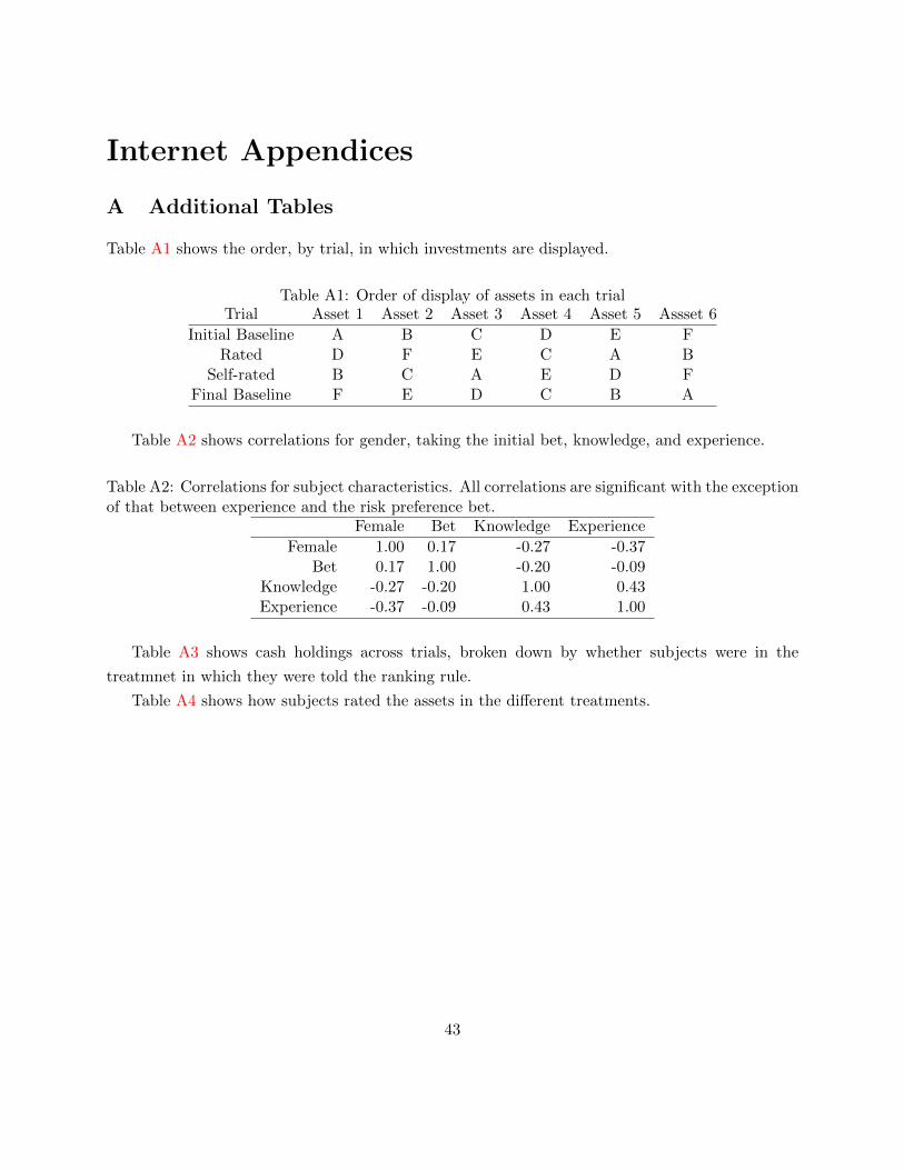
Internet Appendices

A Additional Tables

Table A1 shows the order, by trial, in which investments are displayed.

Table A1: Order of display of assets in each trialTrial Asset 1 Asset 2 Asset 3 Asset 4 Asset 5 Assset 6

Initial Baseline A B C D E FRated D F E C A B

Self-rated B C A E D FFinal Baseline F E D C B A

Table A2 shows correlations for gender, taking the initial bet, knowledge, and experience.

Table A2: Correlations for subject characteristics. All correlations are significant with the exceptionof that between experience and the risk preference bet.

Female Bet Knowledge Experience

Female 1.00 0.17 -0.27 -0.37Bet 0.17 1.00 -0.20 -0.09

Knowledge -0.27 -0.20 1.00 0.43Experience -0.37 -0.09 0.43 1.00

Table A3 shows cash holdings across trials, broken down by whether subjects were in the

treatmnet in which they were told the ranking rule.

Table A4 shows how subjects rated the assets in the different treatments.

43

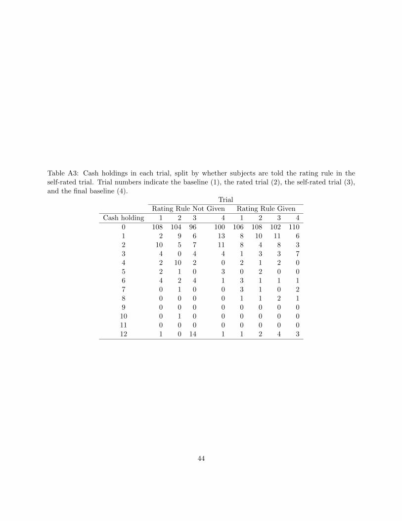
Table A3: Cash holdings in each trial, split by whether subjects are told the rating rule in theself-rated trial. Trial numbers indicate the baseline (1), the rated trial (2), the self-rated trial (3),and the final baseline (4).

TrialRating Rule Not Given Rating Rule Given

Cash holding 1 2 3 4 1 2 3 4

0 108 104 96 100 106 108 102 1101 2 9 6 13 8 10 11 62 10 5 7 11 8 4 8 33 4 0 4 4 1 3 3 74 2 10 2 0 2 1 2 05 2 1 0 3 0 2 0 06 4 2 4 1 3 1 1 17 0 1 0 0 3 1 0 28 0 0 0 0 1 1 2 19 0 0 0 0 0 0 0 010 0 1 0 0 0 0 0 011 0 0 0 0 0 0 0 012 1 0 14 1 1 2 4 3

44

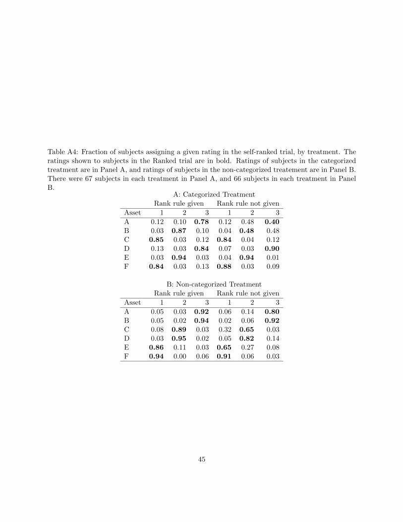
Table A4: Fraction of subjects assigning a given rating in the self-ranked trial, by treatment. Theratings shown to subjects in the Ranked trial are in bold. Ratings of subjects in the categorizedtreatment are in Panel A, and ratings of subjects in the non-categorized treatement are in Panel B.There were 67 subjects in each treatment in Panel A, and 66 subjects in each treatment in PanelB.

A: Categorized TreatmentRank rule given Rank rule not given

Asset 1 2 3 1 2 3

A 0.12 0.10 0.78 0.12 0.48 0.40B 0.03 0.87 0.10 0.04 0.48 0.48C 0.85 0.03 0.12 0.84 0.04 0.12D 0.13 0.03 0.84 0.07 0.03 0.90E 0.03 0.94 0.03 0.04 0.94 0.01F 0.84 0.03 0.13 0.88 0.03 0.09

B: Non-categorized TreatmentRank rule given Rank rule not given

Asset 1 2 3 1 2 3

A 0.05 0.03 0.92 0.06 0.14 0.80B 0.05 0.02 0.94 0.02 0.06 0.92C 0.08 0.89 0.03 0.32 0.65 0.03D 0.03 0.95 0.02 0.05 0.82 0.14E 0.86 0.11 0.03 0.65 0.27 0.08F 0.94 0.00 0.06 0.91 0.06 0.03

45

B Experimental Instructions

Here, we give the text of the Web pages used for this experiment for the baseline treatment.

We footnote the differences between treatments. Separate instruction sets for each treatment are

available by request. Web formatting differed slightly from the formatting below and the Web pages

were interactive. Subjects used drop-down boxes to make allocation decisions and radio buttons to

answer survey questions.

General Instructions

This is an experiment in the economics of decision making. The instructions are simple. If you

follow them carefully and make good decisions, you might earn a considerable amount of money

which will be mailed to you at the end of the experiment.

In stages of this experiment, you will be given cash that you can keep or you can invest all of it

or portions of it in one or more investment alternatives. The amounts you invest in each alternative

and some random draws will determine your payoffs from participating in this experiment. We will

also ask you a series of questions about your preferences, knowledge and demographics.

——— Next Web Page ———

Descriptions of Investment Alternatives

At different stages in this experiment you will be given cash that you can (a) keep or (b) can invest

all of it or portions of it in one or more investment alternatives. This is called an allocation decision.

The amounts you invest will be in $1 increments. Each investment alternative will result in either

a high return or a low return. A random draw will determine which occurs. Half of the time, the

high return will occur and half of the time the low return will occur. The cash you keep always

earns a zero return.

For each $1 invested in an alternative, you will be paid $1 times 1 plus the return that occurs.

Returns will be expressed in percentage terms. So, for example, if the return that occurs is 80%,

you will be paid $1x(1+0.80) = $1.80 for each dollar invested in that alternative. That is, you get

the original $1 back plus 80% of a dollar, or 80 cents in additional return. If the return that occurs

is -30%, then you will be paid $1x(1+(-0.30)) = $0.70. That is, you lose 30%, or 30 cents, of the

original dollar invested. If you had invested $2, you would have been paid $2x(1+0.80) = $3.60 or

$2x(1+(0.30)) = $1.40 if the high or low return had occurred, respectively.

Each investment alternative will be described to you by giving the high return, the low return,

the average return and the range of returns in a table. Finally, you will be given a “Return/Risk”

ratio which is the expected return divided by the range. For example, an investment alternative,

46

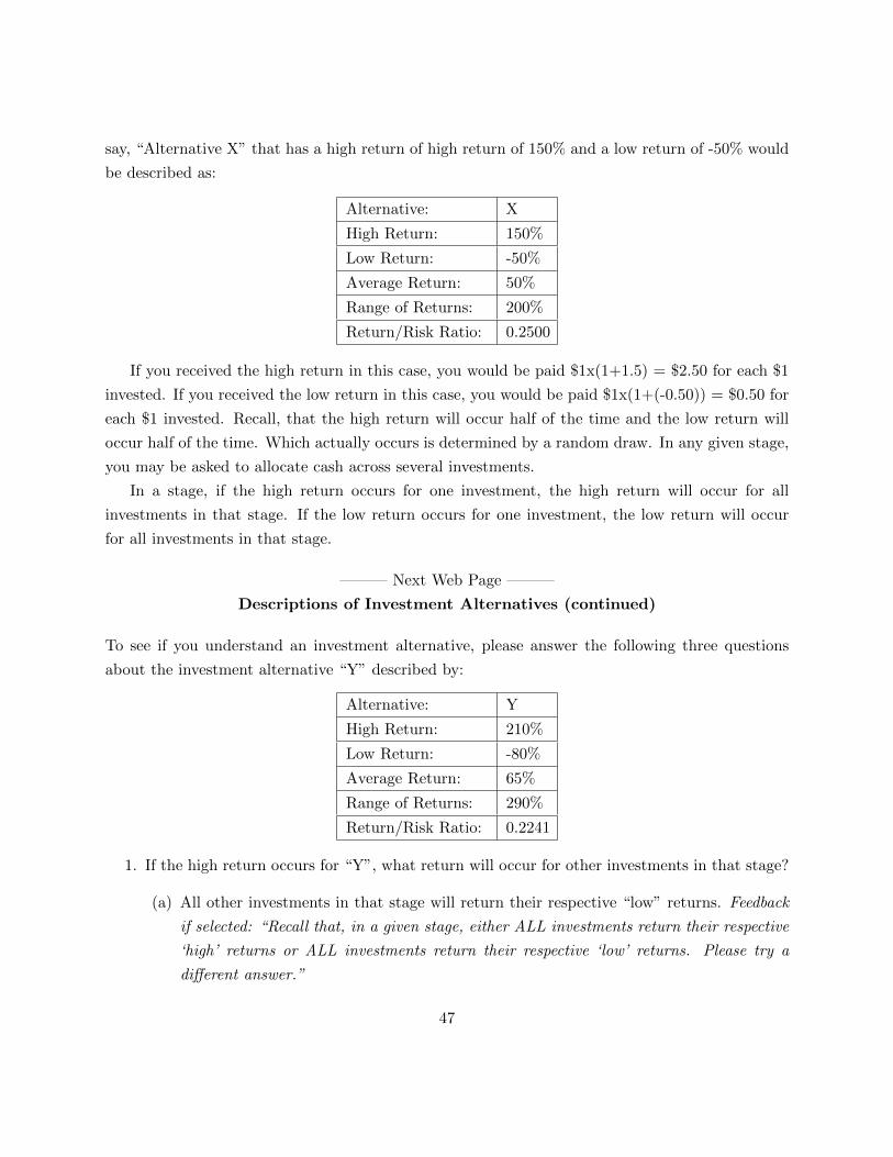
say, “Alternative X” that has a high return of high return of 150% and a low return of -50% would

be described as:

Alternative: X

High Return: 150%

Low Return: -50%

Average Return: 50%

Range of Returns: 200%

Return/Risk Ratio: 0.2500

If you received the high return in this case, you would be paid $1x(1+1.5) = $2.50 for each $1

invested. If you received the low return in this case, you would be paid $1x(1+(-0.50)) = $0.50 for

each $1 invested. Recall, that the high return will occur half of the time and the low return will

occur half of the time. Which actually occurs is determined by a random draw. In any given stage,

you may be asked to allocate cash across several investments.

In a stage, if the high return occurs for one investment, the high return will occur for all

investments in that stage. If the low return occurs for one investment, the low return will occur

for all investments in that stage.

——— Next Web Page ———

Descriptions of Investment Alternatives (continued)

To see if you understand an investment alternative, please answer the following three questions

about the investment alternative “Y” described by:

Alternative: Y

High Return: 210%

Low Return: -80%

Average Return: 65%

Range of Returns: 290%

Return/Risk Ratio: 0.2241

1. If the high return occurs for “Y”, what return will occur for other investments in that stage?

(a) All other investments in that stage will return their respective “low” returns. Feedback

if selected: “Recall that, in a given stage, either ALL investments return their respective

‘high’ returns or ALL investments return their respective ‘low’ returns. Please try a

different answer.”

47

(b) All other investments will return their respective “high” returns. Feedback if selected:

“Correct. Proceed to question 2.”

(c) The returns to other investments at that stage may be mixed with some “high” and some

“low” returns. Feedback if selected: “Recall that, in a given stage, either ALL invest-

ments return their respective ‘high’ returns or ALL investments return their respective

‘low’ returns. Please try a different answer.”

2. If you invest $3 in this alternative and the high return occurs, how much will you be paid?

(a) $2.10 Feedback if selected: “This is the gain on a $1 investment, not the total amount

paid to you. Please try a different answer.”

(b) $3.10 Feedback if selected: “This is the payment for a $1 investment. Recall you are

investing $3. Please try a different answer.”

(c) $6.30 Feedback if selected: “This is the gain on the $3 investment, not the total amount

paid to you. Please try a different answer.”

(d) $9.30 Feedback if selected: “Correct. Please continue to Question 3.”

3. If you invest $2 in this alternative, and the low return occurs, how much will you be paid?

(a) -$0.80 Feedback if selected: “This is the loss on a $1 investment, not the total amount

paid to you. Please try a different answer.”

(b) $0.20 Feedback if selected: “This is the payment for a $1 investment. Recall you are

investing $2. Please try a different answer.”

(c) -$1.60 Feedback if selected: “This is the loss on the $2 investment, not the total amount

paid. Please try a different answer.”

(d) $0.40 Feedback if selected: “Correct. Please continue to the next part of the experiment.”

The continue button only becomes active after the answers are correct.

——— Next Web Page ———

Preliminary Stage

In this stage you have $1 to allocate. You can either keep it or invest it in the following investment

alternative:

48

Alternative: A

High Return: 100%

Low Return: -100%

Average Return: 0%

Range of Returns: 200%

Return/Risk Ratio: 0.0000 Amount Kept

Amount you Invest: =$1-Invested

When you are finished with your choice, click the “continue” button below. At the end of the

experiment, a random draw will determine your payoff to this stage. This will become part of your

earnings for the experiment.

——— Next Web Page ———

Additional Instructions

In the rest of the experiment, you will make several investment decisions. Each decision is a “stage”

in the experiment.

In each stage, you will have $12 to keep or invest. You can keep the $12 or invest some or

all of it in any of 6 investment alternatives in $1 increments. You can invest the $12 in whatever

combination of investments and in whatever amounts you wish so long as the total investment is

less than or equal to $12. Any amount you do not invest will be kept for that stage and earn a zero

return. The outcomes of any given stage will not affect the amount you have to invest in the next

stage. You will always start each stage with a new $12.

At the end of the experiment, we will randomly select one stage . Then, we will make a

SINGLE random draw that will determine whether the gambles in that stage pay the high return

or the low return. That is, either ALL investments in that stage will give you a high return or ALL

of the investments will give the low return.

Earnings from this stage and random draw, together with earnings from the preliminary stage

and the $5 participation fee, will contribute to your earnings for the experiment.

Between stages and at the end of the experiment, you will be asked questions that will help us

categorize your responses.

——— Next Web Page ———

Stage I

In this stage you have $12 to allocate. You can either keep it or invest it in the following

49

investment alternatives in $1 increments.35

Alternative: A B C D E F

High Return: 130% 185% 125% 200% 225% 190%

Low Return: 30% 15% -25% -20% -75% -90%

Average Return: 80% 100% 50% 90% 75% 50%

Range of Returns: 100% 170% 150% 220% 300% 280%

Return/Risk Ratio: 0.8000 0.5882 0.3333 0.4091 0.2500 0.1786 Amount Kept

Amount you Invest: =$12-Invested

Please confirm your allocation before pressing continue.

When you are finished with your choice, click the “continue” button below. At the end of the

experiment, we will randomly select one of these stages to play out. If this stage is chosen, a single

random draw will determine the returns to ALL of the investment in this stage and, as a result,

your payoff to this stage. This will become part of your earnings for the experiment.

——— Next Web Page ———

Stage I Questions36

Please answer the following questions. Click the “Submit” button below to continue on to the

next stage.

1. How satisfied are you with your allocation decision in this stage?

Very Very

Dissatisfied Neutral Satisfied

1 2 3 4 5 6 7

2. Do you wish you could go back and change your decision?

(a) Yes

(b) No

3. How confused did you feel while making the allocation decision?

Very Not Confused

Confused Neutral At All

1 2 3 4 5 6 7

35In treatments with categories, the table of alternatives in each stage was presented with three investments labeled“Category I” on the left and three labeled with “Category II” on the right with a blank column between them. Thesentence “These alternatives have been categorized using a commonly used financial method.” was added to thedescription.

36These questions were asked after each stage. We present them only once here for brevity.’

50

——— Next Web Page ———

Stage II

In this stage you have $12 to allocate. You can either keep it or invest it in the following investment

alternatives in $1 increments. In this stage, we have ranked the investments according to a common

method of ranking investments.37 Investments with more *’s in the ranking line are ranked higher

according to this criterion.

Alternative: A B C D E F

High Return: 200% 190% 225% 125% 130% 185%

Low Return: -20% -90% -75% -25% 30% 15%

Average Return: 90% 50% 75% 50% 80% 100%

Range of Returns: 220% 280% 300% 150% 100% 170%

Return/Risk Ratio: 0.4091 0.1786 0.2500 0.3333 0.8000 0.5882

Ranking: *** * ** * *** ** Amount Kept

Amount you Invest: =$12-Invested

Please confirm your allocation before pressing continue.

When you are finished with your allocation, click the “continue” button below. As a reminder,

at the end of the experiment, we will randomly select one of these stages to play out. If this stage

is chosen, a single random draw will determine the returns to ALL of the investments in this stage

and, as a result, your payoff to this stage.

——— Next Web Page ———

Stage III

In this stage you have $12 to allocate. You can either keep it or invest it in the following

investment alternatives in $1 increments. In this stage, we ask you to first rank the investments.

Use the drop down boxes to assign 1, 2 or 3 stars to investments. 3-star investments should be the

investments with the highest rank, 1-star investments should be the investments with the lowest

rank and 2-star investments should be in between. You are asked to assign two 3-star, two 2-star

37In treatments where the ranking rule is given to subjects, this sentence was replaced with “In this stage, we haveranked the investments according to the Return/Risk ratio, which is a common method of ranking investments.” Thewords “ within categories” were added to the end of the appropriate sentence for treatments with categories.

51

and two 1-star ratings.38

Alternative: A B C D E F

High Return: 185% 125% 130% 225% 200% 190%

Low Return: 15% -25% 30% -75% -20% -90%

Average Return: 100% 50% 80% 75% 90% 50%

Range of Returns: 170% 150% 100% 300% 220% 280%

Return/Risk Ratio: 0.5882 0.3333 0.8000 0.2500 0.4091 0.1786

Ranking: Amount Kept

Amount you Invest: =$12-Invested

When you are finished with your allocation, click the “submit rankings” button below. Then, you

will be allowed to allocate cash.

Please confirm your allocation before pressing continue.

When you are finished with your allocation, click the “continue” button below. As a reminder,

at the end of the experiment, we will randomly select one of these stages to play out. If this stage

is chosen, a single random draw will determine the returns to ALL of the investments in this stage

and, as a result, your payoff to this stage.

——— Next Web Page ———

Stage IV

In this stage you have $12 to allocate. You can either keep it or invest it in the following investment

alternatives in $1 increments.

Alternative: A B C D E F

High Return: 190% 225% 200% 125% 185% 130%

Low Return: -90% -75% -20% -25% 15% 30%

Average Return: 50% 75% 90% 50% 100% 80%

Range of Returns: 280% 300% 220% 150% 170% 100%

Return/Risk Ratio: 0.1786 0.2500 0.4091 0.3333 0.5882 0.8000 Amount Kept

Amount you Invest: =$12-Invested

38In treatments where the ranking rule is given, this paragraph is replaced with “In this stage, we ask you tofirst rank the investments according to the return/risk ratio. Use the drop down boxes to assign 1, 2 or 3 starsto investments. 3-star investments should be the investments with the highest return/risk ratio, 1-star investmentsshould be the investments with the lowest return/risk ratio and 2-star investments should be in between. Youare asked to assign two 3-star, two 2-star and two 1-star ratings.” In both treatments with categories, the lastsentence is replaced with “You are asked to assign one 3-star, one 2-star and one 1-star rating within each categoryof investments.”

52

Please confirm your allocation before pressing continue.

When you are finished with your allocation, click the “continue” button below. As a reminder,

at the end of the experiment, we will randomly select one of these stages to play out. If this stage

is chosen, a single random draw will determine the returns to ALL of the investments in this stage

and, as a result, your payoff to this stage.

——— Next Web Page ———

Knowledge and Demographic Surveys

Next, we would like you to fill out brief demographic and knowledge surveys to help us classify

the data. Your responses will be kept in a data file that does not include any identifying information.

We will keep your participation in this research study confidential to the extent permitted by law.

Taking part in the surveys is completely voluntary. Leave blank any questions you prefer not

to answer. You won’t be penalized or lose any benefits for which you otherwise qualify.

At the end of the surveys, we will randomly select one of stages 1 through 4 that you have

completed and use your allocation decision from this stage and a random draw to determine your

payoffs for this experiment.

Earnings from this stage and random draw, together with earnings from the preliminary stage

and the $5 participation fee, will contribute to your earnings for the experiment.

Press the “continue” button below to go on to the Knowledge Survey.

——— Next Web Page ———

Knowledge Survey

1. How would you classify your knowledge of financial markets?39

(a) No knowledge whatsoever

(b) Beginner level

(c) Intermediate level

(d) Advanced level

2. How much experience have you had with trading on organized financial markets?40

(a) Novice (Have never traded.)

39Source: Variant (added the “No knowledge whatsoever” option) of IEM financial knowledge survey question fromOliven and Rietz (2004).

40Source: IEM financial knowledge survey question from Oliven and Rietz (2004).

53

(b) Limited (Have, for example, made some trades on my own account.)

(c) Experienced Amateur (Have traded a good deal for myself, friends or family.)

(d) Professional (Have been paid for trading.)

3. How many hours in a typical week do you spend following or trading on organized financial

markets?41

(a) None

(b) An hour or less

(c) Between 1 and 5 hours

(d) Between 5 and 10 hours

(e) More than 10 hours.

4. How do you rate your knowledge of investments relative to other people?42

(a) Much less knowledgeable

(b) Somewhat less knowledgeable

(c) About as knowledgeable

(d) Somewhat more knowledgeable

(e) Much more knowledgeable

5. What is compound interest?43

(a) Earning money on your principal and your interest.

(b) a complicated form of interest.

(c) A long term investment.

(d) A risk/return scenario.

6. What is an example of a low risk investment?44

41Source: Variant (made into multiple choice question) of IEM financial knowledge survey question from Olivenand Rietz (2004).

42Source: New.43Source: InvestNative Project Investment Quiz, question 4. http://www.investnative.org/test.html, accessed

08/19/2010.44Source: InvestNative Project Investment Quiz, question 21. http://www.investnative.org/test.html, accessed

08/19/2010.

54

(a) Small cap stock.

(b) High yield “junk” bond.

(c) FDIC insured savings account.

(d) An international mutual fund focused on small Latin American airline companies.

7. If the value of your investment declines by 60%, what subsequent percentage increase is needed

to return to your original investment amount?45

(a) 60%.

(b) 120%.

(c) 150%.

(d) 180%.

8. In general, stock mutual funds that are riskier tend to provide higher returns over time than

stock mutual funds with less risk.46

(a) True.

(b) False.

(c) Don’t know/Not sure.

9. Which of these investments have a risk of losing value?47

(a) Mutual funds

(b) Blue chip stocks

(c) High-yield bonds

(d) They all have risk of losing value

10. What is diversification?48

(a) A way to reduce risk.

45 Source: Pacific Life Investment Knowledge Quiz, question 4: http://www.pacificlife.com/Channel/Educational+Information/Calculators/Investment+Knowledge+Quiz,accessed 08/19/2010.

46Source: Financial Industry Regulatory Authority Investor Knowledge Quiz, question 7:http://apps.finra.org/Quiz/1/investorquiz.aspx, accessed 08/19/2010.

47 Source: Pacific Life Investment Knowledge Quiz, question 5: http://www.pacificlife.com/Channel/Educational+Information/Calculators/Investment+Knowledge+Quiz,accessed 08/19/2010.

48Source: InvestNative Project Investment Quiz, question 11. http://www.investnative.org/test.html, accessed08/19/2010.

55

(b) Investing in different things, such as stocks, bonds, savings, property, etc.

(c) Having an asset allocation that spreads your investment among different asset classes.

(d) All of the above.

11. Common stocks always provide higher returns than bonds or money market investments.49

(a) True.

(b) False.

(c) Don’t know.

12. Asset allocation is a form of:50

(a) Repayment.

(b) Diversification.

(c) Capital.

13. Generally, a portfolio that has 80% of its assets invested in stocks would be best suited for:51

(a) An 18-year-old using the assets to pay for college expenses over the next 4 years.

(b) A 35-year-old investing for retirement.

(c) A 75-year-old investing for income and capital preservation.

(d) None of the above.

(e) Don’t know.

——— Next Web Page ———

Demographic Survey

1. What is your gender?

(a) Female

(b) Male

49Source: Vanguard Investment Knowledge Quiz, question 3: https://personal.vanguard.com/us/InvestmentKnowledge,accessed 08/19/2010.

50Source: InvestNative Project Investment Quiz, question 14. http://www.investnative.org/test.html, accessed08/19/2010.

51Source: Vanguard Investment Knowledge Quiz, question 19: https://personal.vanguard.com/us/InvestmentKnowledge,accessed 08/19/2010.

56

2. What is your age?

(a) Under 30 Years Old.

(b) 30–39 Years Old.

(c) 40–49 Years Old.

(d) 50 Year Old and Older.

3. What is your current marital status?

(a) Married.

(b) Not Married.

4. Do you have children?

(a) Yes.

(b) No.

5. What is your current annual income?

(a) $0–$19,999.

(b) $20,000-$29,999.

(c) $30,000-$39,999.

(d) $40,000-$69,999.

(e) Greater that $60,000.

(f) Would rather not say.

6. What is the highest educational degree you have achieved?

(a) High School

(b) Bachelor’s.

(c) Master’s

(d) Doctorate.

(e) Other.

7. What is or was your college major (most recent degree if you are not currently a student)?

(a) Business.

57

(b) Social Science.

(c) Humanities.

(d) Natural Science.

(e) Mathematics or Engineering.

(f) Other.

(g) None.

——— Next Web Page ———

Final Question

After outcomes and payments have been determined, subjects answer the following final question:

1. How satisfied are you with your allocation decision in the stage that was selected to determine

your payoffs?

Very Very

Dissatisfied Neutral Satisfied

1 2 3 4 5 6 7

58