psicológica universidad de valencia issn (versión impresa ...roden & klein (1972) and hartmann...
TRANSCRIPT
Psicológica Universidad de [email protected] ISSN (Versión impresa): 0211-2159ISSN (Versión en línea): 1576-8597ESPAÑA
2000 Vicenta Sierra / Vicenç Quera / Antoni Solanas
AUTOCORRELATION EFFECT ON TYPE I ERROR RATE OF REVUSKY’S RN TEST:A MONTE CARLO STUDY
Psicológica, año/vol. 21, número 001 Universidad de Valencia
Valencia, España pp. 91-114
Psicológica (2000) 21, 91-114.
Autocorrelation effect on type I error rate of Revusky’s Rn test: A Monte Carlo study
Vicenta Sierra*, Vicenç Quera** and Antoni Solanas**
* ESADE ** Universitat de Barcelona
Monte Carlo simulation was used to determine how violation of the independence assumption affects the empirical probability distribution and Type I error rates of Revusky's Rn statistical test. Simulation results show that the probability distribution of Rn was distorted when the data were autocorrelated. A corrected Rn statistic was proposed to reach a reasonable fit between theoretical (exact) and empirical Type I error rates. We recommend using the corrected Rn statistic when serial dependence in the data is suspected.
Key words: Revusky’s Rn test, Type I error, Monte Carlo simulation, Autocorrelation, Serial dependency, Single-subject designs or N=1 designs.
Both visual inference and statistical analysis have been found
unreliable when data are autocorrelated. Regarding visual inference, Jones, Weinrott & Vaught (1978) pointed to the distorting effects of serial dependency on the interpretation of data, showing that autocorrelation was responsible for the discrepancies between inferences based on a visual analysis and those resulting from statistical analysis. The problem was aggravated in those cases having an evident change of level. More important is the low agreement found among judges, which reveals the inadequacy of visual analysis and the need to apply more objective procedures. Another aspect to be considered is the training of judges. Wampold & Furlong (1981) found differences in the interpretation of data between a group of judges trained in multivariable techniques and another group trained in visual analysis. These differences consisted in that the former could detect intervention effects far better as they paid more attention to the relative variations in the scores, while the latter attached more importance to level and slope changes between phases in a time series.
* Correspondence concerning this article should be addressed to Vicenta Sierra, ESADE. Address: ESADE. Avda. de Pedralbes, 60-62. 08034 Barcelona, Spain. [email protected]
92 V. Sierra et al.
Due to their assumptions, classic statistical tests (e.g., ANOVA, t-test, chi-square test, etc.) are not suitable for analyzing data with serial dependency (Scheffé, 1959; Toothaker, Banz, Noble, Camp & Davis, 1983). This autocorrelation affects the level of significance of the statistical tests under or overestimating Type I error rates. A first attempt to solve the problem of serial dependency is found in Shine & Bower (1971). Gentile, Roden & Klein (1972) and Hartmann (1974) were later to propose other models based on classic statistical tests, unsuccessfully however, due to the restrictive conditions these models required. These strategies are founded on the analyses of variance. A factor is added in order to extract the variability assigned to serial dependency.
Faced with the problems of using the classic tests for behavioral designs, alternative techniques were recommended. Thus, randomization tests (Edgington, 1967, 1980) enable behavioral designs to be analyzed using classic statistical tests. Revusky's (1967) Rn statistic permits behavioral data to be analyzed in multiple baseline designs. The binomial-based graph-statistical technique proposed by White (1974), termed Split-middle, allows analysis of designs A-B, A-B-A and their extensions. Crosbie (1987) warns that the Split-middle technique must be used with caution when serial dependency in the data is suspected (specifically, positive dependency increase Type I error rate, and negative dependency decrease it). Wolery & Billingsley (1982) propose joint application of the Split-middle technique and the Rn statistic, in order to determine not only the statistical significance in level changes but also slope changes in multiple baseline designs.
A test devised for studying serial dependency (an aspect not considered by previous techniques) is the interrupted time series analysis. Initially developed by Box & Tiao (1965), Box & Jenkins (1970), it was later adapted to the social and behavioral sciences by Glass, Wilson & Gottman (1975). This analysis would appear to be an adequate alternative to the problem of serial dependency among observations; the minimum requirement of 50 data per phase to carry out the analysis, combined with the difficulties involved in identifying the autoregressive model, are two of the most problematic aspects of using this technique (Harrop & Velicer, 1985).
The tests dealt with so far attempt to solve the problem of serial dependency on the assumption that it has no effect (randomization tests, Rn, etc.) or is removed (interrupted time series analysis). Nevertheless, obtaining the level of significance of a statistic based on a distribution function that assumes independence between scores is a debatable method. Suffice it to mention some of the results that show how the empirical Type I
Revusky’s RN test 93
error rate does not concur with the nominal rate when data are autocorrelated (Crosbie, 1987, 1989, 1993; Gardner, Hartmann & Mitchell, 1982; and Toothaker et al.,1983).
Considering that nonparametric statistics do not always guarantee the elimination of the effect of autocorrelation on the Type I error rate, we analyzed the effect of serial dependency on the Rn statistic. Multiple baseline designs require not only an analysis of magnitude and the sign of the autocorrelation in calculating the statistic, but also an essential analysis of the interaction of the different levels of autocorrelation in each design. The aim of this paper is to demonstrate that the violation of the assumption of independence affects the Rn statistic and to provide a corrective action based on the dispersion of the series. Empirical and theoretical Type I error rates are not identical when Rn statistic is obtained in series where there exist different autocorrelation parameter values. It is an expected result because Rn statistic assumes independence among series. The discrepancy between empirical and theoretical Type I error rates is explained by different series’ variance. As a consequence, series comparability is not guaranteed. To reach comparability among series, we propose a Rn statistic correction that extracts autocorrelation effect on variability. A way to accomplish this goal is to standardize the data. We therefore generated data by Monte Carlo simulation under various extreme experimental conditions (varying the autocorrelation of the series) and compared the Rn statistic calculated from the original data (uncorrected Rn statistic) with that calculated from the data transformed by the proposed correction method (corrected Rn statistic).
DESCRIPTION OF REVUSKY'S RN STATISTIC A set of k series of data is recorded for k objects (subjects, behaviors
or situations) in a multiple baseline design; in other words, k independent subexperiments exist. The main purpose of multiple baseline designs is to probe the effectiveness of treatment (Figure 1). In the first subexperiment, an experimental object is chosen at random and treatment is introduced, the rest of the objects acting as a control group. The scores obtained by all the objects at the time the treatment is introduced (or, alternatively, the mean scores for each phase) are ordered in such a way that each object is assigned a rank (ranging from one to k) according to its performance level. The result of the subexperiment is the rank obtained by the experimental object. The experimental object is discarded for the remainder of the analysis. A second experimental object is then chosen at random from amongst the k-1 control objects. The new experimental object is subjected to the same treatment while the remaining k-2 objects act as controls. Now the scores of the
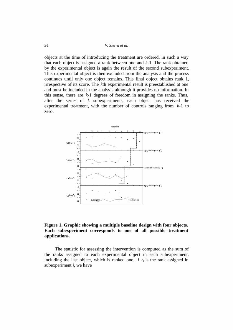
94 V. Sierra et al.
objects at the time of introducing the treatment are ordered, in such a way that each object is assigned a rank between one and k-1. The rank obtained by the experimental object is again the result of the second subexperiment. This experimental object is then excluded from the analysis and the process continues until only one object remains. This final object obtains rank 1, irrespective of its score. The kth experimental result is preestablished at one and must be included in the analysis although it provides no information. In this sense, there are k-1 degrees of freedom in assigning the ranks. Thus, after the series of k subexperiments, each object has received the experimental treatment, with the number of controls ranging from k-1 to zero.
Figure 1. Graphic showing a multiple baseline design with four objects. Each subexperiment corresponds to one of all possible treatment applications.
The statistic for assessing the intervention is computed as the sum of
the ranks assigned to each experimental object in each subexperiment, including the last object, which is ranked one. If ri is the rank assigned in subexperiment i, we have
Revusky’s RN test 95
∑=
k
iin r=R
1
The Rn statistic represents the sum of k discrete values ri and takes integer values between k and k(k+1)/2. Furthermore, random selection of the experimental objects and their subsequent exclusion from the analysis ensures statistical independence between the ri obtained in each subexperiment. Assuming null hypothesis, the Rn statistic is distributed symmetrically with expectancy
( ) ( ) ( )341
121
1
+=
+−= ∑
=kkikRE
k
in
and variance
( )( ) ( )∑=
+−−+−+−=
k
in ikikikR
1
2241
322261
)(var
as has been shown in Cronholm & Revusky (1965). In a multiple baseline designs where k subexperiments have been
carried out and assuming independence among subexperiments, Rn statistic’s distribution is
!
#)( 1
k
jrxRP
x
kj
k
ii
n
∑ ∑= =
=
=≤
For example, if k=4, Rn statistics takes values between 4 and 10. The probability that Rn ≤ 5 is equal to
24
#)5()4()5(
5
4
4
1∑ ∑
= =
=
==+==≤ j ii
nnn
jrRPRPRP
Rn = 4 is only obtained when ri = 1 in each subexperiment. If Rn = 5, the possible values of ri in the subexperiments are: (r1 = 1, r2 = 1, r3 = 2, r4 =1); (r1 = 1, r2 = 2, r3 = 1, r4 =1); and (r1 = 2, r2 = 1, r3 = 1, r4 =1).
METHOD A modular program was created in Fortran 77, running on a HP -UX
system, for data generation and Rn statistic calculation. In the data generation process, NAG Mark-15 mathematical-statistical libraries were used (specifically the external libraries G05CCF and G05FDF).
96 V. Sierra et al.
Data Generation: Data were generated using the following expression: .t x = ttkt .....,,=+x ++ 2111 ερ (1)
where ρk represents the autocorrelation parameter for the object (or series) k, and εi were N(0,1) random variables. For each call to the NAG libraries 600 data (εi) were generated, independently for all objects which composed a single multiple baseline design. For each of the series the first 75 data were discarded in order to reduce artificial effects (Greenwood & Matyas, 1990), that is, to attenuate as far as possible the effect of anomalous initial values (seeds) of the pseudo-random generator and stabilize the series. Each series is interpreted as an A-B design where the length of A phase (or baseline) is five for the first subexperiment, increasing by 15 data for each of the remaining subexperiments. The B phase (or intervention ph ase) has a constant length of 10 data for each of the subexperiments. No trend or level change between phases was programmed when generating the data. Two types of multiple baseline design were planned depending on the number of objects they had (four or five series per design). The numbers of objects that compose the design determine the significance levels for the Rn statistic. Thus, with four objects per design we can reach significance levels of 0.05, while five is the minimum number of objects necessary for obtaining significance levels of 0.01 (Revusky, 1967). The exact Type I error rates corresponding to the extremes values of Rn statistic for four and five object are α= 0.04167 and α= 0.00833, respectively, using formulae provided by Revusky (1967).
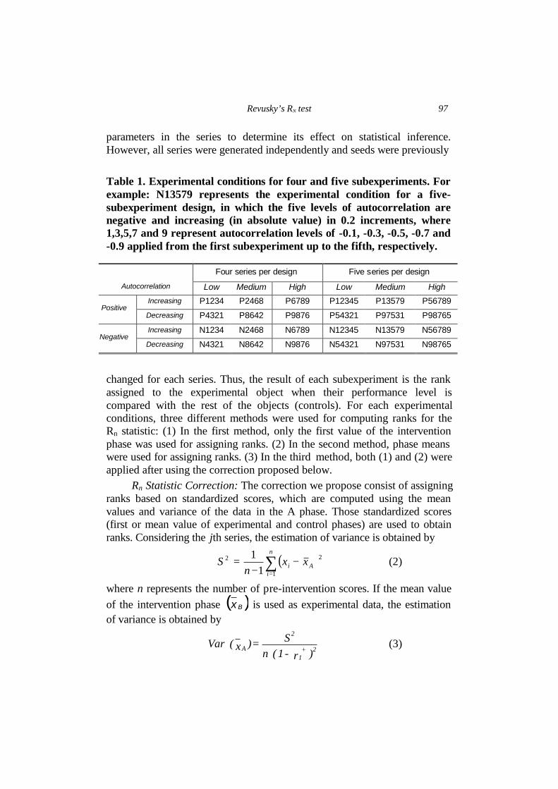
Different theoretical levels of autocorrelation were established between -0.9 and 0.9, increasing by 0.1 or 0.2. The level of autocorrelation applied to the data series defined the experimental condition of each design size. Considering that each series ha s a different autocorrelation level, the experimental conditions are defined in accordance with: a) the sign of the autocorrelation levels (all positive levels or all negative, denoted by P and N, respectively) and b) increasing or decreasing autocorrelation levels (considered as an absolute value) assigned to the successive applications of the treatment. Combining autocorrelation levels, and sign and number of subexperiments, 12 experimental conditions were chosen (Table 1).
Experimental objects in each subexperiment were selected in a systematic manner, i.e. in the first subexperiment the first series is used as the experimental object, in the second subexperiment the second, and so on up to the fourth/fifth subexperiment with the fourth/fifth series as an experimental object. Experimental objects were not selected randomly because it was necessary to keep a specific arrangement of autocorrelation
Revusky’s RN test 97
parameters in the series to determine its effect on statistical inference. However, all series were generated independently and seeds were previously Table 1. Experimental conditions for four and five subexperiments. For example: N13579 represents the experimental condition for a five-subexperiment design, in which the five levels of autocorrelation are negative and increasing (in absolute value) in 0.2 increments, where 1,3,5,7 and 9 represent autocorrelation levels of -0.1, -0.3, -0.5, -0.7 and -0.9 applied from the first subexperiment up to the fifth, respectively.
Four series per design Five series per design Autocorrelation Low Medium High Low Medium High
Increasing P1234 P2468 P6789 P12345 P13579 P56789 Positive
Decreasing P4321 P8642 P9876 P54321 P97531 P98765 Increasing N1234 N2468 N6789 N12345 N13579 N56789
Negative Decreasing N4321 N8642 N9876 N54321 N97531 N98765
changed for each series. Thus, the result of each subexperiment is the rank assigned to the experimental object when their performance level is compared with the rest of the objects (controls). For each experimental conditions, three different methods were used for computing ranks for the Rn statistic: (1) In the first method, only the first value of the intervention phase was used for assigning ranks. (2) In the second method, phase means were used for assigning ranks. (3) In the third method, both (1) and (2) were applied after using the correction proposed below.
Rn Statistic Correction: The correction we propose consist of assigning ranks based on standardized scores, which are computed using the mean values and variance of the data in the A phase. Those standardized scores (first or mean value of experimental and control phases) are used to obtain ranks. Considering the jth series, the estimation of variance is obtained by
( )∑=
−−
=n
iAi xx
nS
1
22
11 (2)
where n represents the number of pre-intervention scores. If the mean value of the intervention phase ( )Bx is used as experimental data, the estimation of variance is obtained by
)r - 1( nS = )x( Var
21+
2
A (3)

98 V. Sierra et al.
where S2 is calculated via equation (2), and the lag-1 autocorrelation coefficient (r1
+) is estimated using the following correction (Huitema & McKean, 1991):
)x - x(
)x - x( )x - x( = r
n1
+ r = r
Ai2
n
1 =i
A1+iAi
1-n
1 =i1
1+1
∑
∑ (4)
For short series, r1+ yields poor estimates of the true autocorrelation in
the data. On the other hand, for a multiple baseline design mo re precise autocorrelation estimates are obtained as larger baseline sizes are achieved when considering successive subexperiments.
According to the size of the design involved (four or five subexperiments), the Rn statistic will have discrete values belonging to intervals [4,10] and [5,15], respectively. Under the null hypothesis, Rn is distributed symmetrically around its expected value, which equals 7 and 10. Expected variances are 2.1666 and 4.1664, respectively.
According to Robey & Barcikowski (1992), the number of simulations necessary for detecting deviations from the exact Type I error rate under the criterion α ± 1/4α, a Type I error rate ω = 0.01, and a priori power 1-β = 0.9, is 6109 for four subexperiments (α = 0.04167) and 31739 for five subexperiments (α = 0.00833). Forty thousand simulations were generated by experimental condition in order to surpass the minimum power levels specified above.
Data Analysis: Goodness of fit between theoretical frequencies and data obtained via simulation was assessed using a χ2 test. To ascertain whether the empirical Type I error rate matches the exact value, confidence interval ranges for Type I error rate reliability ranges were obtained using the criterion α ± 1/4α (where α represents the exact Type I error rate described above for the two design sizes).
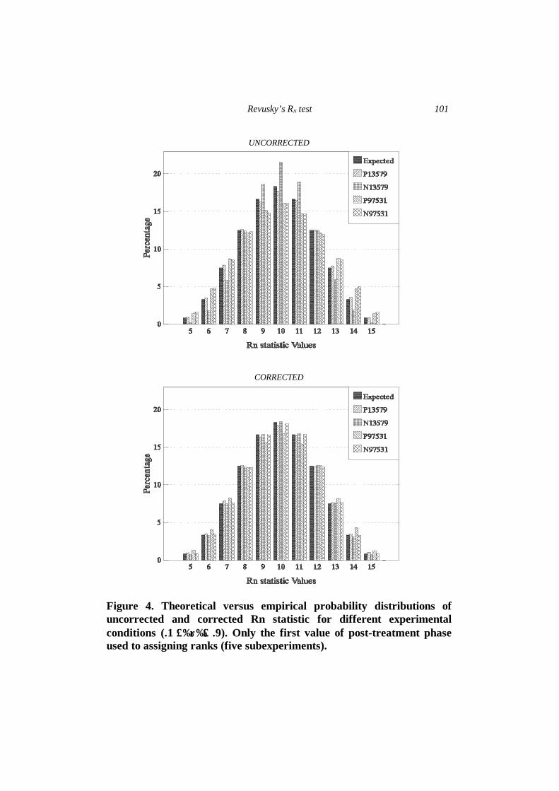
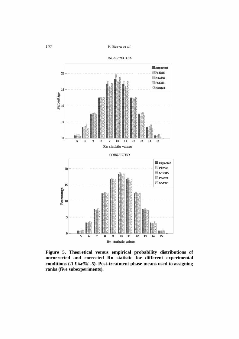
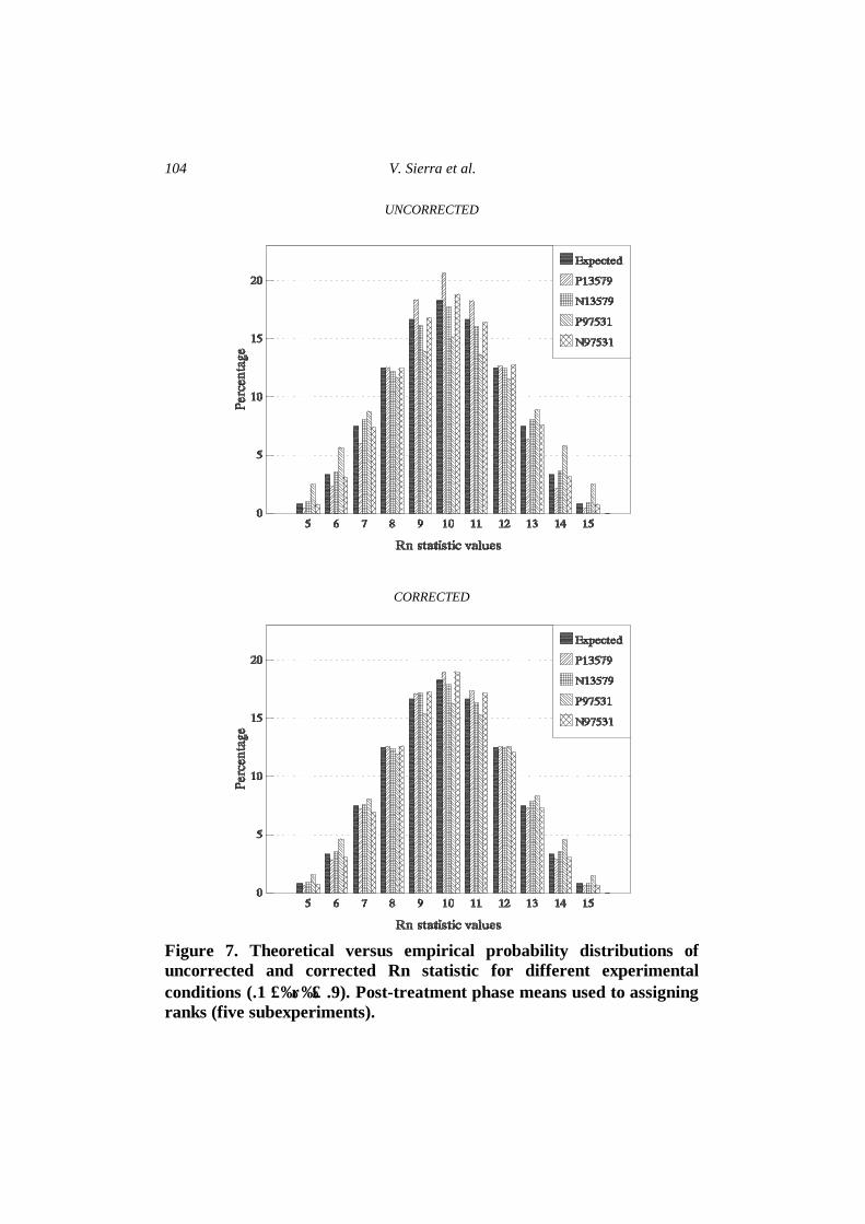
RESULTS Results obtained for five- and four-series designs were virtually
identical. Reference will therefore only be made to the results of the analysis of five series designs. Figures 2, 3, 4, 5, 6, and 7 show the theoretical and
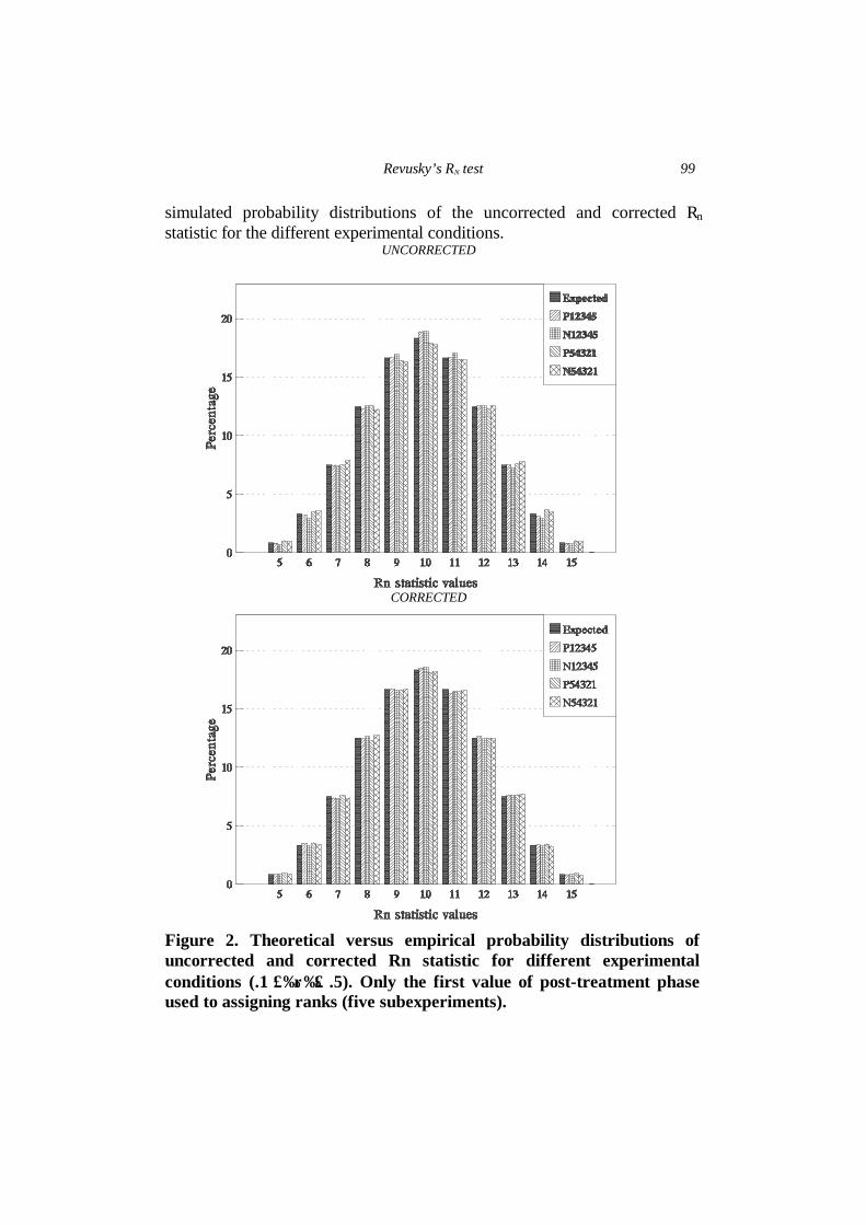
Revusky’s RN test 99
simulated probability distributions of the uncorrected and corrected Rn statistic for the different experimental conditions.
UNCORRECTED
CORRECTED
Figure 2. Theoretical versus empirical probability distributions of uncorrected and corrected Rn statistic for different experimental conditions (.1 ≤ρ≤ .5). Only the first value of post-treatment phase used to assigning ranks (five subexperiments).

100 V. Sierra et al.
UNCORRECTED
CORRECTED
Figure 3. Theoretical versus empirical probability distributions of uncorrected and corrected Rn statistic for different experimental conditions (.5 ≤ρ≤ .9). Only the first value of post-treatment phase used to assigning ranks (five subexperiments).
Revusky’s RN test 101
UNCORRECTED
CORRECTED
Figure 4. Theoretical versus empirical probability distributions of uncorrected and corrected Rn statistic for different experimental conditions (.1 ≤ρ≤ .9). Only the first value of post-treatment phase used to assigning ranks (five subexperiments).
102 V. Sierra et al.
UNCORRECTED
CORRECTED
Figure 5. Theoretical versus empirical probability distributions of uncorrected and corrected Rn statistic for different experimental conditions (.1 ≤ρ≤ .5). Post-treatment phase means used to assigning ranks (five subexperiments).

Revusky’s RN test 103
UNCORRECTED
CORRECTED
Figure 6. Theoretical versus empirical probability distributions of uncorrected and corrected Rn statistic for different experimental conditions (.5 ≤ρ≤ .9). Post-treatment phase means used to assigning ranks (five subexperiments).
104 V. Sierra et al.
UNCORRECTED
CORRECTED
Figure 7. Theoretical versus empirical probability distributions of uncorrected and corrected Rn statistic for different experimental conditions (.1 ≤ρ≤ .9). Post-treatment phase means used to assigning ranks (five subexperiments).
Revusky’s RN test 105
With respect to the effect of serial dependency on the empirical Type I error rate, it can be seen that the magnitude and the sign of the autocorrelation levels together with the interaction between the different autocorrelated levels (increasing or decreasing) affects in a different manner and degree, underestimating or overestimating the probabilities associated with the extreme values of the Rn statistic. All the experimental conditions show symmetry around the mean value, and the mean values are equal t o the theoretically expected. Variances are very different to those expected, due to the effect of the violation of the assumption of independence between scores.
Tables 2, 3, 4, and 5 provide the values of variance, chi-square test, and empirical Type I error rates for extreme values of Rn statistic under the different experimental conditions. A greater proximity is detected between the empirical rate and the exact Type I error rate under conditions with absolute autocorrelation levels varying between 0.1 and 0.5. As for the distribution tails, although the probabilities obtained remain quite close to the expected values, conditions having autocorrelations assigned in increasing order tend to underestimate the Type I error rate, and those with decreasing autocorrelations tend to overestimate it. This result (irrespective of the use of a first value or the mean of the post-treatment data) becomes evident with greater |?| levels.
When a single post-treatment score is used for assigning ranks with the uncorrected Rn statistic, Type I error rates are underestimated in those conditions having series with negative autocorrelation levels, between - 0.1 and - 0.9, in increasing order (in absolute value). On the other hand, decreasing series of both signs (P97531, N97531, P98765, and N98765) overestimate the Type I error rate in those conditions having high autocorrelation levels.
Considering the mean of the data in the phases, the results show very similar patterns to those obtained by using a single post-treatment value. That is to say the Type I error rate is underestimated when autocorrelation levels are assigned in increasing order, and is overestimated when they are assigned in decreasing order. When autocorrelations varied in the 0.1 and 0.9 range, Type I error rates tended to overestimate or underestimate the exact rates (under the criterion α ± 1/4α). Concerning the adjustment between empirical and theoretical probability distributions, the test used (χ2) show significant differences (p < 0.05) between most experimental conditions and the pattern of expected results.
106 V. Sierra et al.
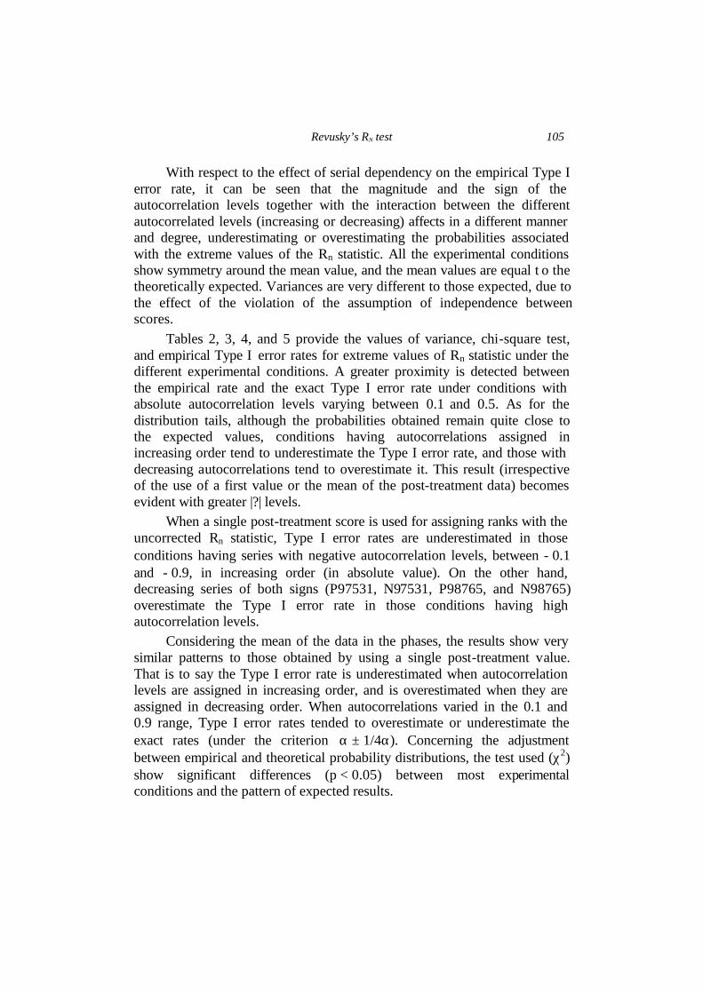
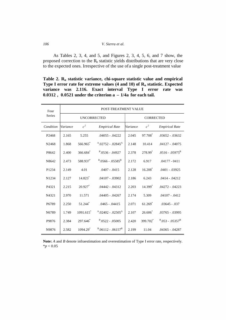
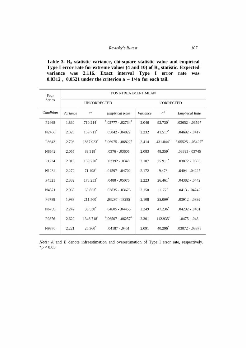
As Tables 2, 3, 4, and 5, and Figures 2, 3, 4, 5, 6, and 7 show, the proposed correction to the Rn statistic yields distributions that are very close to the expected ones. Irrespective of the use of a single post-treatment value Table 2. Rn statistic variance, chi-square statistic value and empirical Type I error rate for extreme values (4 and 10) of Rn statistic. Expected variance was 2.116. Exact interval Type I error rate was 0.0312 ÷ 0.0521 under the criterion α ± 1/4α for each tail.
POST-TREATMENT VALUE Four Series
UNCORRECTED CORRECTED
Condition Variance χ2 Empirical Rate Variance χ2 Empirical Rate
P2468 2.165 5.255 .04055 - .04222 2.045 97.708* .03652 - .03632
N2468 1.868 566.965* A.02752 - .02845A 2.148 10.414 .04127 - .04075
P8642 2.400 366.684* B.0536 - .04927 2.378 278.99* .0516 - .05975B
N8642 2.473 588.937* B.0566 - .05585B 2.172 6.917 .04177 - 0411
P1234 2.149 4.01 .0407 - .0415 2.128 16.208* .0401 - .03925
N1234 2.127 14.823* .04107 - .03902 2.186 6.243 .0414 - .04212
P4321 2.215 20.927* .04442 - .04312 2.203 14.399* .04272 - .04223
N4321 2.970 11.571 .04405 - .04267 2.174 5.309 .04107 - .0412
P6789 2.250 51.244* .0465 - .04415 2.071 61.269* .03645 - .037
N6789 1.749 1091.615* A.02402 - .02505A 2.107 26.606* .03765 - .03995
P9876 2.384 297.646* B.0522 - .05005 2.420 399.702* B.053 - .05357B
N9876 2.582 1094.29* B.06112 - .06157B 2.199 11.04 .04365 - .04287
Note: A and B denote infraestimation and overestimation of Type I error rate, respectively. *p < 0.05
Revusky’s RN test 107
Table 3. Rn statistic variance, chi-square statistic value and empirical Type I error rate for extreme values (4 and 10) of Rn statistic. Expected variance was 2.116. Exact interval Type I error rate was 0.0312 ÷ 0.0521 under the criterion α ± 1/4α for each tail.
POST-TREATMENT MEAN Four
Series UNCORRECTED CORRECTED
Condition Variance χ2 Empirical Rate Variance χ2 Empirical Rate
P2468 1.830 710.214* A.02777 - .02734A 2.046 92.730* .03652 - .03597
N2468 2.320 159.711* .05042 - .04822 2.232 41.517* .04692 - .0417
P8642 2.703 1887.923* B.06975 - .06822B 2.414 431.844* B.05525 - .05427B
N8642 2.055 89.318* .0376 - .03605 2.083 48.359* .03393 - 03745
P1234 2.010 159.720* .03392 - .0348 2.107 25.911* .03872 - .0383
N1234 2.272 71.498* .04597 - .04702 2.172 9.473 .0404 - .04227
P4321 2.332 178.253* .0488 - .05075 2.223 26.461* .04382 - .0442
N4321 2.069 63.853* .03835 - .03675 2.150 11.770 .0413 - .04242
P6789 1.989 211.500* .03297- .03285 2.108 25.009* .03912 - .0392
N6789 2.242 36.530* .04605 - .04455 2.249 47.236* .04292 - .0461
P9876 2.620 1348.718* B.06507 - .06257B 2.301 112.935* .0475 - .048
N9876 2.221 26.360* .04187 - .0451 2.091 40.296* .03872 - .03875
Note: A and B denote infraestimation and overestimation of Type I error rate, respectively. *p < 0.05.
108 V. Sierra et al.
Table 4. Rn statistic variance, chi-square statistic value and empirical Type I error rate for extreme values (5 and 15) of Rn statistic. Expected variance was 4.166. Exact interval Type I error rate was 0.00625 ÷ 0.0104 under the criterion α ± 1/4α for each tail.
POST-TREATMENT VALUE Five
Series UNCORRECTED CORRECTED
Cond. Variance χ2 Empirical Rate Variance χ2 Empirical Rate
P13579 4.294 32.068* .0096 - .00852 4.307 35.972* .00935 - .0099
N13579 3.138 1602.710* A.00232 - .00227A 4.103 13.864 .00767 - .00775
P97531 5.070 1240.465* B.01442 - .0144B 4.751 525.614 B.01295 - .01245B
N97531 5.182 1605.139* B.0164 - .01592B 4.219 9.846 .00867- 00847
P12345 4.078 19.136* .00767 - .00775 4.188 9.418 .00845 - .00807
N12345 3.961 71.660* .00685 - .00762 4.157 4.373 .00832 - .0086
P54321 4.330 52.570* .01007 - .01015 4.275 21.523* .00932 - .0094
N54321 4.321 36.733* .0091 - .00917 4.173 9.522 .00877 - .0078
P56789 4.265 24.715* .00895 - .00897 3.952 76.780* .00675 - .00655
N56789 3.264 1297.019* A.00325 - .0035A 4.044 37.970* .00765 - .00817
P98765 4.750 530.024* B.01332 - .01232B 4.656 371.930* B.0112 - .01122B
N98765 5.126 1431.952* B.01607 - .015B 4.237 28.051* .00912 - .00845
Note: A and B denote infraestimation and overestimation of Type I error rate, respectively *p < 0.05.
Revusky’s RN test 109
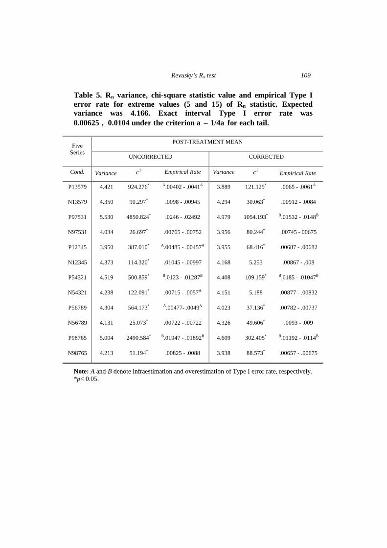
Table 5. Rn variance, chi-square statistic value and empirical Type I error rate for extreme values (5 and 15) of Rn statistic. Expected variance was 4.166. Exact interval Type I error rate was 0.00625 ÷ 0.0104 under the criterion α ± 1/4α for each tail.
POST-TREATMENT MEAN Five
Series UNCORRECTED CORRECTED
Cond. Variance χ2 Empirical Rate Variance χ2 Empirical Rate
P13579 4.421 924.276* A.00402 - .0041A 3.889 121.129* .0065 - .0061A
N13579 4.350 90.297* .0098 - .00945 4.294 30.063* .00912 - .0084
P97531 5.530 4850.824* .0246 - .02492 4.979 1054.193* B.01532 - .0148B
N97531 4.034 26.697* .00765 - .00752 3.956 80.244* .00745 - 00675
P12345 3.950 387.010* A.00485 - .00457A 3.955 68.416* .00687 - .00682
N12345 4.373 114.320* .01045 - .00997 4.168 5.253 .00867 - .008
P54321 4.519 500.859* B.0123 - .01287B 4.408 109.159* B.0185 - .01047B
N54321 4.238 122.091* .00715 - .0057A 4.151 5.188 .00877 - .00832
P56789 4.304 564.173* A.00477- .0049A 4.023 37.136* .00782 - .00737
N56789 4.131 25.073* .00722 - .00722 4.326 49.606* .0093 - .009
P98765 5.004 2490.584* B.01947 - .01892B 4.609 302.405* B.01192 - .0114B
N98765 4.213 51.194* .00825 - .0088 3.938 88.573* .00657 - .00675
Note: A and B denote infraestimation and overestimation of Type I error rate, respectively. *p< 0.05.

110 V. Sierra et al.
or the mean value of the intervention phase data, this correction minimizes the serial dependency effect of underestimating Type I error rate. For confidence intervals centered on the exact rate, only the decreasing series that were assigned positive autoregressive levels were significant. In addition, when the correction is used, less experimental conditions differ significantly from the expected distributions, according to χ2 (p < 0.05).
DISCUSSION This Monte Carlo study shows the effects produced by the violation of
the assumption of independence among scores, confirming the results obtained by other researchers on the study of serial dependency and its effect on statistical inference. Certain studies (Box, 1954; Crosbie, 1987; 1989; 1993; Gardner, Hartmann & Mitchell, 1982; Scheffé, 1959; Toothaker et al, 1983) have yielded similar results. Statistics such as the t -test, the binomial test applied to the Split-middle technique, the C statistic, the ANOVA and the χ2 test give acceptable results only when the scores have moderate levels of serial dependency. On the other hand, positive autocorrelation overestimates the Type I error rate, and negative autocorrelation underestimates it.
This investigation questioned whether the Rn statistic is robust against the violation of the assumption of independence. An analysis of the effect of serial dependence on the statistic was carried out, considering not only magnitude and sign of the autocorrelation levels, but also the interaction between different dependency levels of the series involved in their calculation. When identical autocorrelation levels and sign exist, the distribution of the statistic is not effected by presence of autocorrelation in the series (as statistical theory might predict). The same results are obtained when autocorrelation levels are identical but have alternate positive and negative signs. Likewise, Rn shows a highly acceptable pattern of results (although with significant disagreement with respect to the expected values when subjected to the χ2 test) when the series have autocorrelation levels between - 0.5 and 0.5.
Opposite results in accordance with the sign and the increase/decrease of the autocorrelation levels involved in the series have been observed. Parallel to the results described above, the most extreme results are obtained with high autocorrelation levels (0.5 ≤ |ρk| ≤0.9) where the increasing series overestimate and the decreasing series underestimate the error rates. The difference between the increasing and decreasing patterns can be explained by how autocorrelation affects the variance of the series. Given

Revusky’s RN test 111
( ) 2
2
1 ρσ−
=kxVar (5)
the highest variance is obtained when autocorrelation is extreme (in absolute value), for a constant value of σ2. This explains why series with monotonically decreasing autocorrelation yield a larger proportion of extreme Rn values (overestimation of the Type I error rate) than that expected at random on the assumption of independence. For series with monotonically increasing autocorrelation, the results are reversed, and a larger proportion of central values of Rn is obtained, that is, the exact Type I error rate is underestimated. In addition, as equation (5) shows, the variance of the series does not depend on the sign of the autocorrelation. As equation (5) is asymptotic, this independence can only be observed when sample size, or number of scores in the series, is big.
Using only the initial score of the treatment phase is not a common practice. Obviously, this strategy refers to an extreme case, as it is unusual to have a single measurement in the B phase. In some experiments, only one or few scores are available in the intervention phase, for example, as mentioned by Revusky (1967) for the application of lethal drugs. The most common practice is to assess the intervention in terms of average performance over several time-points, instead of doing so in terms of a level change when intervention is first introduced. Comparing results obtained by means of the uncorrected procedure, the same pattern of results can be observed. As was to be expected, when using the mean, the conditions in which a negative autoregressive component was introduced are less sensitive to the effect of the violation of the assumption of independence (the negative autocorrelation effect generates series with alternating values, distributed symmetrically around the mean of the series). Comparatively, in series with positive autocorrelation, the presence of predominantly increasing or decreasing runs imply that a high number of sequences are biased with respect to the mean, especially when sample size is small. Consequently, when calculating the mean of the intervention phase, those series that are affected by negative autocorrelation provide an estimation closer to the mean level of the series than those affected by positive autocorrelation. When calculating Rn, experimental conditions affected by negative autocorrelation yield results that are closer to what is expected when scores are independent than conditions affected by positive dependency.
As serial dependency affects the variability in the series, a correction based on the deviation shown by the data should improve the adjustment of the empirical Type I error rate to the exact rate. Prior analysis carried out on
112 V. Sierra et al.
the proposed correction for Rn revealed that, in series without serial dependency, the correction did not alter the empirical Type I error rate, which remained at the expected levels on the assumption of independence (Sierra, 1997). These results can also be observed in series with identical autocorrelation levels, whether positive or negative; the same results were obtained when the autocorrelations were identical but their signs where alternate. Under none of the conditions analyzed in this study was an unfavorable result detected after applying the correction to Rn. The corrected Rn statistic always fits better both the empirical and expected Rn statistic probability distribution than the uncorrected one. Therefore, we recommend the correction whenever serial dependence in the data is suspected. Before calculating Rn, it is advisable to check for serial dependence. When no increasing or decreasing autocorrelation values correspond to the order of application of the intervention, treatment effect can be assessed by the uncorrected Rn statistic; otherwise transforming the data routinely by means of the proposed correction is recommended. The aim is not to cancel out the distorting effects caused by the existence of serial dependence, but to improve the adjustment of the empirical Type I error rate to the exact rates.
We should underline the reliable results obtained when studying the violations of the assumption of independence on the Rn statistic. Disagreements regarding the expected distribution have only been reported in a set of conditions that can be considered extreme, as obtaining those extreme patterns after random application of the treatment is u nlikely. In short, although levels of disagreement between the empirical and exact Type I error rate continue to exist (particularly in positive autocorrelation patterns) the proposed correction increases the robustness of the technique against the violation of the assumption of independence.
RESUMEN Efecto de autocorrelación sobre la tasa de error tipo I del estadístico Rn de Revusky: Una simulación Monte Carlo. Mediante simulación Monte Carlo se analizan los efectos que la violación del supuesto de independencia provocan sobre la tasa de error Tipo I, en el estadístico Rn de Revusky. Los resultados de la simulación muestran la distorsión de la distribución de probabilidad del estadístico Rn cuando los datos presentan dependencia serial. Se propone y analiza una corrección del estadístico Rn que mitigue las diferencias entre los valores exactos y empíricos de la tasa de error Tipo I. Por sus favorables resultados recomendamos aplicar la corrección propuesta siempre que se sospeche de la existencia de dependencia serial en los datos.
Revusky’s RN test 113
Palabras clave: Estadístico Rn de Revusky; Error Tipo I; Simulación Monte Carlo; Autocorrelación; Dependencia Serial; Diseño de caso único; Diseño N=1.
REFERENCES Box, G. E. P. (1954). Some theorems on quadratic forms applied in the study of analysis of
variance problems: II. Effect of inequality of variance and correlation. Annals of Mathematical Statistics, 25, 484-498.
Box, G. E. P. & Jenkins, G. M. (1970). Time-Series analysis: Forescating and control. San Francisco: Holden-Day.
Box, G. E. P. & Tiao, G. C. (1965). A change in level of a non stationary time series. Biometrika, 52, 181-192.
Cronholm, J. N. & Revusky, S. H. (1965). A sensitive rank test for comparing the effects of two treatments on a single group. Psychometrika, 30, 4, 459-467.
Crosbie, J. (1987). The inability of the binomial test to control Type I error with single-subject data. Behavioral Assessment, 9, 141-150.
Crosbie, J. (1989). The inappropriateness of the C statistics for assessing stability or treatment effects with single-subject data. Behavioral Assessment, 11, 315-325.
Crosbie, J. (1993). Interrupted time-series analysis with brief single-subject data. Journal of Consulting and Clinical Psychology, 61, 966-974.
Edgington, E. S. (1967). Statistical inference N=1 experiments. The Journal of Psychology, 65, 195-199.
Edgington, E. S. (1980). Randomization Tests. New York: Marcel Dekker. Gardner, W., Hartmann, D. P. & Mitchell, C. (1982). The effects of serial dependence on
the use of χ2 for analyzing sequential data in dyadic interactions . Behavioral Assessment, 4, 75-82.
Gentile, J. R., Roden, A. H. & Klein, P. D. (1972). An analysis of variance model for the intrasubject replication test. Journal of Applied Behavioral Analysis, 5, 193-198.
Glass, G. V., Wilson, V.L. & Gottman, J. M. (1975). Design and analysis of time series experiments. Boulder. CO: Colorado Associated University Press.
Greenwood, K. M. & Matyas, T. A. (1990). Problems with application of interrupted time series analysis for brief single-subject data. Behavioral Assessment, 12, 355-370.
Harrop, J. W. & Velicer, W. F. (1985). A comparison of alternative approaches to the analysis of interrupted time-series. Multivariate Behavioral Research, 20, 27-44.
Hartman, D. P. (1974). Forcing square pegs into round holes: Some comments on an analysis-of-variance model for the intrasubject replication design. Journal of Applied Behavior Analysis, 7, 635-638.
Huitema, B.E. & McKean, J.W. (1991). Autocorrelation estimation and inference with small samples. Psychological Bulletin, 110, 291-304.
Jones, R. R., Weinrott, M. R. & Vaught, R. S. (1978). Effects of serial dependency on the agreement between visual and statistical inference . Journal of Applied Behavior Analysis, 11, 277-283.
Matyas, T. A. & Greenwood, K. M. (1991). Problems in the estimation of autocorrelation in brief time series and some implications for behavioral data . Behavioral Assessment, 13, 137-157.
114 V. Sierra et al.
Robey, R. R. & Barcikowski, R. S. (1992). Type I error and the number of iterations in Monte Carlo studies of robustness. British Journal of Mathematical and Statistical Psychology, 45, 283-288.
Revusky, S. H. (1967). Some statistical treatments compatible with individual organism methodology. Journal of the Experimental Analysis of Behavior, 19, 319-330.
Scheffé, H. (1959). The analysis of variance. New York: Wiley. Shine, L. C. & Bower, S. M. (1971). A one-way analysis of variance for single-subject
designs. Educational and Psychological Measurement, 31, 105-113. Sierra, V. (1997). Estadísticos robustos en diseños conductuales: Análisis y simulación
Monte Carlo. Doctoral Thesis. University of Barcelona. Toothaker, L. E., Banz, M., Noble, C., Camp, J. & Davis, D. (1983). N=1 Designs: The
failure of anova-based tests. Journal of educational statistics, 8, 289-309. Wampold, B. E. & Furlong, M. J. (1981). The heuristics of visual inference. Behavioral
Assessment, 3, 79-92. Wolery, M. & Billingsley, F. F. (1982). The application of Revusky's Rn test to slope and
level changes. Behavioral Assessment, 4, 93-103. White, O. R. (1974). The Split-Middle: A quickie method of trend stimation. Experimental
Education Unit, Child Development and Mental Retardation Center. University of Washington, Seattle.
(Manuscrito recibido:7/10/99; Revisión aceptada: 21/3/00 )