l -4vol. 25 (3), 2006 - limnetica · limnetica-4vol. 25 (3), 2006 ... mapa de la parte continental...
TRANSCRIPT
LIMNETICA -4Vol. 25 (3), 2006
INDICE
BARBOUR, MICHAEL T., SUSAN HOLDSWORTH AND STEVE PAULSEN. Using Ecological Data as a Foundation for Decision-Making in the USA. . . . . . . . . . . . . . . . . . . . . . . . . . . . . . . . . . . . . . . . . . . . . . . . . . . . . . . . . . . . . . . . . . . . . . . . . . . . . . . . . . . . . . . . . . . 613
MARIA M. BARON-RODRIGUEZ, ROSA A. GAVILAN-DIAZ Y JOHN J. RAMIREZ RESTREPO. Variabilidad espacial y temporal enla comunidad de cladoceros de la Cienaga de Paredes (Santander, Colombia) a lo largo de un ciclo anual . . . . . . . . . . . . . . 623
I. ANNE, I., M. L. FIDALGO, L. THOSTHRUP AND K. CHRISTOFFERSEN. Influence of filtration and glucose amendment onbacterial growth rate at different tidal conditions in the Minho Estuary River (NW Portugal) . . . . . . . . . . . . . . . . . . . . . . . . . 637
BOUTERFAS, RADIA, MOUHSSINE BELKOURA, ALAIN DAUTA. The effects of irradiance and photoperiod on the growth rate ofthree freshwater green algae isolated from a eutrophic lake . . . . . . . . . . . . . . . . . . . . . . . . . . . . . . . . . . . . . . . . . . . . . . . . . . . . . . . 647
GODINHO, FRANCISCO NUNES AND MARIA TERESA FERREIRA. Influence of habitat structure on the fish prey consumption bylargemouth bass, Micropterus salmoides, in experimental tanks . . . . . . . . . . . . . . . . . . . . . . . . . . . . . . . . . . . . . . . . . . . . . . . . . . . 657
MARTINOY, MONICA, DANI BOIX, JORDI SALA, STEPHANIE GASCON, JAUME GIFRE, ALBA ARGERICH, RICARD DE LA BARRERA,SANDRA BRUCET, ANNA BADOSA, ROCIO LOPEZ-FLORES, MONTSERRAT MENDEZ, JOSEP MARIA UTGE AND XAVIER D.QUINTANA. Crustacean and aquatic insect assemblages in the Mediterranean coastal ecosystems of Emporda wetlands(NE Iberian peninsula) . . . . . . . . . . . . . . . . . . . . . . . . . . . . . . . . . . . . . . . . . . . . . . . . . . . . . . . . . . . . . . . . . . . . . . . . . . . . . . . . . . . . . . . . 665
OSCOZ JAVIER, FRANCISCO CAMPOS Y Ma CARMEN ESCALA. Variacion de la comunidad de macroinvertebrados bentonicos enrelacion con la calidad de las aguas . . . . . . . . . . . . . . . . . . . . . . . . . . . . . . . . . . . . . . . . . . . . . . . . . . . . . . . . . . . . . . . . . . . . . . . . . . . . 683
GONZALEZ DEL TANAGO, MARTA Y DIEGO GARCIA DE JALON. Propuesta de caracterizacion jerarquica de los rıos espanolespara su clasificacion segun la Directiva Marco de la Union Europea . . . . . . . . . . . . . . . . . . . . . . . . . . . . . . . . . . . . . . . . . . . . . . . 693
MAIA, HUGO M. S., CARLA F. Q. MAIA, DANIEL F. C. PIRES AND ALEXANDRE C. N. VALENTE. Biology of the iberian chub(Squalius carolitertii) in an atlantic-type stream (river Lima basin-north Portugal). A preliminary approach . . . . . . . . . . . . 713
ORTEGA, FERNANDO, GEMA PARRA Y FRANCISCO GUERRERO. Usos del suelo en las cuencas hidrograficas de los humedalesdel Alto Guadalquivir: Importancia de una adecuada gestion . . . . . . . . . . . . . . . . . . . . . . . . . . . . . . . . . . . . . . . . . . . . . . . . . . . . . . 723
MARTINEZ-BASTIDA, JUAN JOSE, MERCEDES ARAUZO M. Y MARIA VALLADOLID. Diagnostico de la calidad ambiental del rıoOja (La Rioja, Espana) mediante el analisis de la comunidad de macroinvertebrados bentonicos . . . . . . . . . . . . . . . . . . . . . . 733
VALLADOLID, MARIA, JUAN JOSE MARTINEZ-BASTIDA, MERCEDES ARAUZO Y CARMEN GUTIERREZ. Abundancia y biodiversi-dad de los macroinvertebrados del rıo Oja (La Rioja, Espana) . . . . . . . . . . . . . . . . . . . . . . . . . . . . . . . . . . . . . . . . . . . . . . . . . . . . . 745
ARAUZO, MERCEDES, MARIA VALLADOLID, JUAN JOSE MARTINEZ-BASTIDA Y CARMEN GUTIERREZ. Dinamica espacio-temporaldel contenido en nitrato de las aguas superficiales y subterraneas de la cuenca del rıo Oja (La Rioja, Espana):Vulnerabilidad del acuıfero aluvial . . . . . . . . . . . . . . . . . . . . . . . . . . . . . . . . . . . . . . . . . . . . . . . . . . . . . . . . . . . . . . . . . . . . . . . . . . . . . 753
GALOTTI, A., F. JIMENEZ-GOMEZ Y F. GUERRERO. Estructura de tamanos de las comunidades microbianas en sistemasacuaticos salinos del alto Guadalquivir . . . . . . . . . . . . . . . . . . . . . . . . . . . . . . . . . . . . . . . . . . . . . . . . . . . . . . . . . . . . . . . . . . . . . . . . . 763
SERAFIM, ANTONIO, MANUELA MORAIS, PEDRO GUILHERME, PAULA SARMENTO, MANUELA RUIVO AND ANA MAGRICO. Spatialand temporal heterogeneity in the Alqueva reservoir, Guadiana river, Portugal . . . . . . . . . . . . . . . . . . . . . . . . . . . . . . . . . . . . . . 771
TRACANNA, BEATRIZ, C., S. N. MARTINEZ DE MARCO, M. J. AMOROSO, N. ROMERO, P. CHAILE AND A. MANGEAUD. Physical,chemical and biological variability in the Dr. C. Gelsi reservoir (NW Argentine): A temporal and spatial approach . . . . . 787
MONINO-FERRANDO, A., ENRIQUE MORENO-OSTOS AND LUIS CRUZ-PIZARRO. Phytoplankton patchiness in two shallowwaterbodies . . . . . . . . . . . . . . . . . . . . . . . . . . . . . . . . . . . . . . . . . . . . . . . . . . . . . . . . . . . . . . . . . . . . . . . . . . . . . . . . . . . . . . . . . . . . . . . . . . 809
MORENO, J. L., C. NAVARRO Y J. DE LAS HERAS. Propuesta de un ındice de vegetacion acuatica (IVAM) para la evaluacion delestado trofico de los rıos de Castilla-La Mancha: Comparacion con otros ındices bioticos . . . . . . . . . . . . . . . . . . . . . . . . . . . . 821
BARBOUR, MICHAEL T., JAMES B. STRIBLING AND PIET F.M. VERDONSCHOT. The Multihabitat Approach of USEPA’s RapidBioassessment Protocols: Benthic Macroinvertebrates . . . . . . . . . . . . . . . . . . . . . . . . . . . . . . . . . . . . . . . . . . . . . . . . . . . . . . . . . . . . 839

Limnetica, 25 (3): xx-xx (2006)Limnetica, 25 (3): 613-622 (2006)c© Asociacion Espanola de Limnologıa, Madrid. Spain. ISSN: 0213-8409
Using Ecological Data as a Foundation for Decision-Making in the USA
Michael T. Barbour1,∗, Susan Holdsworth2, and Steve Paulsen3
1 Center for Ecological Sciences. Tetra Tech, Inc. 10045 Red Run Blvd., Suite 110. Owings Mills, MD 21117.USA Email: [email protected] Office of Wetlands, Oceans and Watersheds. US Environmental Protection Agency. 1200 Pennsylvania Avenue,NW (4503 T). Washington, DC 20460. USA3 Aquatic Monitoring and Assessment Branch. Western Ecology Division, NHEERL, ORD, EPA200 S.W. 35th St. Corvallis, OR 97330. USA3 Aquatic∗ Corresponding author.
ABSTRACT
Using Ecological Data as a Foundation for Decision-Making in the USA
Decisions that impact the quality of aquatic systems are being made daily throughout the world based on little or no ecologicalinformation (Barbour et al., 2004). Monitoring information, based on scientifically and rigorously tested ecological indicators,is integral to water quality management programs for protecting human health, preserving and restoring ecosystem integrity,and sustaining a viable economy. Under the Clean Water Act of the United States, water quality agencies of the states andtribes are required to conduct monitoring and assessment to address the mandates of the law. However, recent critiques ofwater monitoring programs have claimed that the United States Environmental Protection Agency (U.S. EPA) and State waterquality agencies cannot make statistically valid inferences about water quality and the condition of the Nation’s waters, i.e.,whether they are improving, degrading or remaining the same; furthermore, we lack data to support management decisionsregarding the Nation’s aquatic resources. The National Wadeable Streams Assessment Program (WSA) was established inearly 2004 to answer the question of what is the status of the Nation’s waters, and to maximize partnerships among U.S. EPA,States and Tribes, and other agencies to establish a framework to address issues at state and local scales. Ecological data in anyform require some measure of translation to be useable by the environmental manager, i.e., a hierarchy exists in the translationprocess from basic biological data in its rawest form through a series of manipulations in the analysis phase to reporting ofthe results and interpretation. This nationally focused program is a step towards ensuring adequate monitoring data exist inthe future to assess water quality and make sound watershed management decisions throughout the USA; actions are takento protect and restore water quality that maximize benefits and minimize costs; and sound science forms the basis of makinginformed decisions regarding our aquatic resource.
Key words: Communicating science, biological integrity, environmnetal monitoring, Clean Water Act, stream assessment,reference condition, ecoregion, stressor-response, ecological assesment.
RESUMEN
Utilizando la informacion ecologica como base para la tarea de decisiones en los Estados Unidos
Diariamente se estan tomando decisiones que inciden en la calidad de los sistemas acuaticos basadas en escasa o ningunainformacion ecologica (Barbour et al., 2004). La informacion obtenida en programas de gestion, basada en indicadorescientıficos y basados en indicadores ecologicos, se integra en programas de gestion de la calidad del agua para la proteccionde la salud humana, la preservacion o restauracion de la integridad de los ecosistemas y el sostenimiento de una economıaviable. Por mandato del Acta sobre el Agua Limpia de los Estados Unido, se han creado agencias a nivel de Estados oregiones para realizar programas de estudio y gestion para cumplir el mandato de la ley. No obstante, recientemente hansurgido crıticas a los programas de gestion senalando que la Agencia de Proteccion Ambiental de los Estados Unidos (U.S.EPA) y las agencias de calidad del agua estatales no pueden realizar inferencias estadısticamente validas acerca de la calidaddel agua y de la situacion de las aguas de la nacion, p. e. si estan mejorando, degradando o permanecen igual. Ademas, notenemos datos para apoyar las decisiones de gestion en relacion con los recursos acuaticos nacionales. El Programa deEstudio de los Rıos Vadeables (WSA) se establecio en 2004 para responder a la pregunta de cual es la situacion de las aguasde la nacion, y para maximizar la colaboracion entre U.S. EPA, y las agencias estatales, locales y similares para realizar unmarco de trabajo que permita establecer los objetivos a escalas estatal y local. La informacion ecologica de cualquier tipo

614 Barbour et al.
requiere algunas medidas de traduccion para que sea utilizable por los gestores ambientales, p. e. existe una jerarquıa en elproceso de traslacion desde datos biologicos basicos, en su forma poco elaborada, hasta una serie de manipulaciones en lafase de analisis para los informes de resultados y su interpretacion. Este programa enfocado a nivel nacional es un paso paraasegurar que existen datos adecuados de gestion a traves de todo el paıs. Se estan realizando actuaciones para proteger ymejorar la calidad del agua que maximice los beneficios y minimice los costes a la vez que establezcan las bases cientıficaspara tomar decisiones teniendo en cuenta nuestros recursos acuaticos.
Palabras clave: Transmision del conocimiento cientıfico, integridad biologica, gestion ambiental, Acta sobre el Agua Limpia,informacion sobre los rıos, ecoregion, factor estresante-tipo de respuesta, estudio ecologico.
INTRODUCTION
The 21st century will witness greater attentionto water resource restoration, protection, andmanagement. As the global demand for adequatesupplies of clean water has escalated, so haveconcerns about public health and environmentalquality (Barbour et al., 2004). There is evidencethe increased demands have taken a tollon aquatic ecosystems. Ecological informationobtained in the latter half of the 20th century hasuncovered a serious decline in aquatic ecosystemhealth (Karr, 1995; Master et al., 1998).Decisions that impact the quality of aquaticsystems are being made daily throughout theworld based on little or no ecological information(Barbour et al., 2004). Monitoring information,based on scientifically and rigorously testedecological indicators, is integral to water qualitymanagement programs for protecting humanhealth, preserving and restoring ecosystemintegrity, and sustaining a viable economy.
In the United States of America (USA),the Clean Water Act (CWA) of 1972 servesas the regulatory impetus for the restorationand maintenance of physical, chemical, andbiological integrity (Fig. 1) as the long-termgoal of environmental protection for aquaticresources (Adler, 1995). The sum of these threeaspects constitutes the concept of ecologicalintegrity, which is inherent in the water lawsof most countries (Barbour et al., 2000).Under the CWA, the states are required toconduct monitoring and assessment to addressthe mandates of the law. In addition, FirstNations, or Native American tribal authorities,have similar jurisdictional requirements as the
states (Barbour & Gerritsen, 2006). Therefore,a multitude of water resource agencies existin the USA to accomplish the stipulatedregulations. Recent critiques of water monitoring
Figure 1. The Ecological Integrity goal of the US CleanWater Act where Ecological Integrity is a culmination ofBiological, Physical, and Chemical Integrity. La consecucionde la Integridad Ecologica de la Acta sobre Aguas Limpias delos US es la culminacion de la integridad biologica, fısica yquımica.
programs have claimed that the United StatesEnvironmental Protection Agency (U.S. EPA)and State water quality agencies cannot makestatistically valid inferences about water qualityand the condition of the Nation’s waters,i.e., whether they are improving, degrading orremaining the same; furthermore, we lack datato support management decisions regarding the

Using Ecological Data as a Foundation for Decision-Making in the USA 615
Figure 2. Map of the continental United States, showing ecoregions (a) and jurisdictional boundaries of U.S. EPA regions (b).Mapa de la parte continental del los Estados Unidos mostrando las ecoregiones (a) y las fronteras jurisdiccionales de las regionsU.S. EPA.
Nation’s aquatic resources. These critiques havestemmed from reviews of the U.S. GeneralAccounting Office (2000), the National ResearchCouncil (2001), the Heinz Center Report (2002),
and most recently, the draft Report on theEnvironment (EPA, 2003). The primary reasonsfor this inability to produce adequate reportingof ecological condition are (1) the monitoring

616 Barbour et al.
designs used by water quality agencies targetspecific problems or waterbodies, which cannotbe aggregated to accurately describe conditionsacross the country, and (2) the question ofcomparability among the agencies of the datagathering tools, which, to date, have precludedaggregating data and/or assessments for regionaland national scales.
THE NATIONAL WADEABLE STREAMSASSESSMENT PROGRAM
The diverse geomorphologic land-forms and cli-matological regions of the USA underscore theimportance of regional specificity in faunal dis-tributions and composition (Barbour & Yoder,2000). However, the basic premise of a bioas-sessment approach remains similar across thecountry. Therefore, a versatile method for sam-pling, and data interpretation, is needed that willprovide some consistency in otherwise disparateareas of rainfall, temperature, and geology (Bar-bour & Gerritsen, 2006).
The National Wadeable Streams AssessmentProgram (WSA) was established in early 2004 toanswer the question posed by the U.S. Congress,that is, what is the status of the Nation’swaters. A secondary issue, and perhaps the mostimportant for long-term sustainability, is for theWSA to maximize partnerships among U.S. EPA,States and Tribes, and other agencies by usingthe best combination of monitoring tools andstrategies to answer key environmental questionsat national, and regional scales, and to establisha framework to address issues at state andlocal scales. U.S. EPA’s strategy for effectivelytargeting water quality actions that maximizesbenefits and saves costs focuses on four keyaspects, i.e., strengthen State programs, promotepartnerships, use multiple monitoring tools, andexpand accessibility and use of data.
The basic framework of WSA builds uponprevious large-scale programs, such as the Envi-ronmental Monitoring and Assessment program(EMAP) of the U.S. EPA, and uses existingstate agency expertise and knowledge of aquaticresources. Randomly generated sampling loca-
tions stratified by ecoregion (Level II; see Omer-nik 1987) and U.S. EPA region (Figs. 2a andb) enables reporting at regional scales. StandardOperating Procedures (SOPs) and a strict QualityAssurance Program is used to ensure the highestdata integrity for the assessment. The data collec-tion from 600 stream sites in the western USA(U.S. EPA Regions 8-10) over a four year period(2001-2004) complements the sampling of 500stream sites in 2004 throughout USEPA Regions1-7 (Fig. 2b). A report to the U.S. Congress isscheduled for December 2006.
SAMPLING SURVEY DESIGN OFTHE WSA
The choice of a particular monitoring surveydesign should be based on the monitoring ob-jectives and ultimate decision process incum-bent upon the outcome of the study. Any well-designed monitoring and assessment program isinherently anticipatory in that it will provide in-formation for present needs and those not yet de-termined (Yoder & Rankin, 1995). The funda-mental challenge, given our inability to sampleevery lake and stream in the country, is how toselect a subset of sites that can be used to inferconditions for all aquatic systems (Hughes et al.,2000). To obtain unbiased estimates of condition,the agencies now often use probability samplesurveys. Sites or streams are selected using stra-tified random techniques such that the collectionof sample sites is representative of the resourcepopulation of interest. Thus, one can make infe-rences from the survey results to the entire po-pulation. In the USA, streams are identified byresource type, i.e., intermittent, perennial, etc.,and further stratified by size to obtain a frame-work for randomizing the streams to be sampledin the resource population of interest. This de-sign is cost effective in that the entire resourcedoes not have to be sampled –only a represen-tative set of streams. This sampling design wasdeveloped by EMAP and has been used to assessthe ecological status of waters on different scalesof basin, statewide, regional, and national levels(Paulsen & Linthurst, 1994; Hughes et al., 2000).
Using Ecological Data as a Foundation for Decision-Making in the USA 617
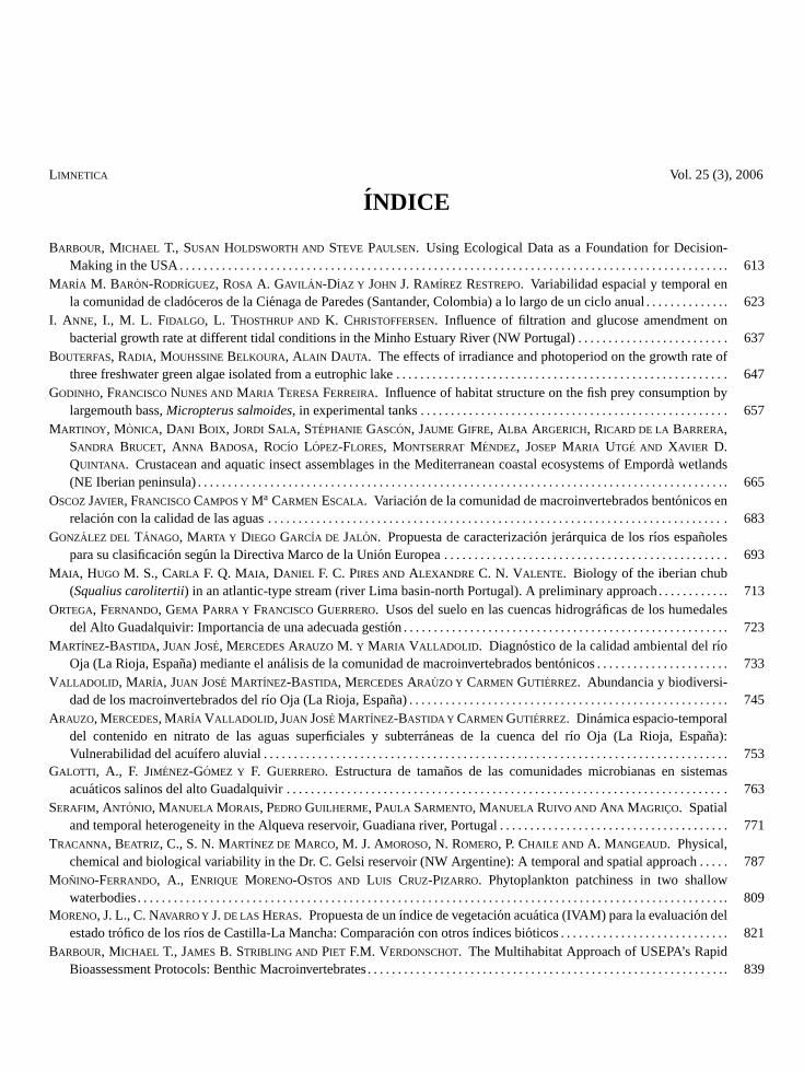
Descriptive Statistics Interpreted Statistics
Figure 3. Data analysis process from descriptive statistics to interpretation. Proceso de analisis de datos desde la descripcionestadıstica hasta la interpretacion.
Answering two basic questions is the goal ofthe WSA: (1) What percentage of the nation’swadeable streams resource is in good condition?And, (2) What is the relative importanceof stressors as evaluated in the WSA? Foraddressing the first question, information fromthe stream biota, i.e., the macroinvertebrateassemblage for the WSA, forms the basis ofthe assessment. The endpoint is based on ourknowledge of reference conditions that serveas the basis for deriving relevant thresholdsfor making condition assessments (Fig. 3).The second question requires that we haveinformation on the key stressors derived fromchemical, physical, biological and watersheddata, that might be affecting the overallecological condition of the water resource invarious parts of the USA. The estimate of theextent of stressors throughout the water resourcealong with the relationship between the stressorsand biological indicators provide some sense ofthe cause of degraded waters (Fig. 4).
ESTABLISHINGREFERENCECONDITIONSAS BENCHMARKS FOR THE WSA
In the USA, we stress the importance of establi-shing strict criteria on the physical characteristicsof catchments and streams to serve as referencesites (Barbour & Gerritsen, 2006). Many indivi-dual nations, and the European Union as a whole,have codified the concept of reference conditionin legislation aimed at protecting and improvingthe ecological condition of running waters (Stod-dard et al., 2006). However, the selection of refe-rence criteria is often a mixture of data analysisand professional judgment. Reference sites oughtto be derived from streams that represent mini-mally disturbed conditions in each region (Bai-ley et al., 2004). For the WSA, short-term ob-jectives were established to quickly characterizethe background biological expectations of the va-rious regions by using a combination of samplinga select few reference streams provided by thestates, use of existing state biological data from

618 Barbour et al.
Figure 4. Example of inferences that will be drawn from the probability sampling to answer the basic questions of the WSA.Ejemplo de inferencia que puede se dibujado desde el muestreo probabilıstico hasta responder preguntas basicas de la WSA.
their ecoregions, and consensus-based decisionsregarding appropriate indicators and endpoints.
The short-term process to establish referenceconditions for the WSA is based on theuse of reference sites across the country andentails the following:
• Use a combination of sampling (this fieldseason) at targeted reference sites that arederived from state data, analysis of existingstate data where appropriate, and consensus-based decisions of expected values of selectedendpoints (also derived from state databasesand expert knowledge).
• Select approximately 10 best reference sitesto be sampled this year for each ecore-gion (Level II), based on recommendationsobtained from state databases. Selection ofsites within an ecoregion will also considersome stratification by certain characteristics,such as elevation, catchment size, etc.,where possible. Convene a technical expertworkgroup to develop a consensus-basedframework for background from existing stateand federal programs. Use results from thesubset of reference sites sampled this year incombination with other appropriate data andinformation to aid in establishing supportablebenchmarks for the assessment.
Results from sampling the small subset of10 sites/ecoregion with the same methods willenable our developing a notion of range andvariability within a small subset of least disturbedsites, and assist in identifying other candidatereference sites from within the random samplesurvey. This population of reference sites isconsidered to be minimal and insufficient forfull calibration of indicators, but is intendedfor approximations of benchmarks for endpoints,given the coarse reporting unit of EcoregionLevel II. To supplement this information, we usedexisting state and federal data, where possible,to help develop a framework for expectationsof ecological conditions. The Technical ExpertWorkgroup will meet on several occasions todiscuss the best approach to develop a frameworkfor assessment. Part of the discussions wasdevoted to indicators and endpoints that will formthe basis of the assessment for the final report.
COMMUNICATING THE SCIENCE FORDECISION-MAKING
To answer the questions set forth for the WSA,reporting or communicating the results and re-commendations is the underpinnings of the entirestudy. Effective communication of assessment re-

Using Ecological Data as a Foundation for Decision-Making in the USA 619
Land UseSource(s)
BiologicalResponse
Figure 5. Conceptual relationship of human activities or land use, stressors, and response indicators (D. Allan, personalcommunication). Relaciones conceptuales de las actividades humanas o uso del suelo, factores perturbadores y indicadores dela respuesta de dichos efectos (D. Allan, comunicacion personal).
Figure 6. Hierarchy of data manipulation and translationfrom basic biological data to making informed decisions.Jerarquıa del procesado de los datos y su transferencia desdedatos biologicos basicos hasta la toma de decisiones teniendoen cuenta dicha informacion.
sults is critical to making scientifically soundand socially meaningful decisions (Preston etal., 2004). The model for translating thescientific findings into useable information fordecision-makers relates objectives, measurableattributes (indicators), and testable hypothesesthat help answer the assessment’s questions(Stevenson et al., 2004). Three fundamental
categories of variables should be communicatedto environmental managers: response, stressor,and human activity variables (Fig. 5). Responsevariables are measures or indicators of the valuedecological attributes that are directly relatedto management goals, program objectives, andecosystem services (Stevenson et al., 2004).Response variables are similar in conceptto assessment endpoints as defined by Suter(1990). Stressors are the physical, chemical,and biological factors that affect responses.Human activity variables describe the spatialand temporal extent of human activities in awatershed, as well as their intensity (Stevensonet al., 2004). Stevenson et al. (2004) pointout that the response, stressor, and humanactivity categories of variables are fundamentalbecause of their roles in managing ecosystems.Human activities produce the contaminants andhabitat alterations (stressors) that affect valuedattributes. Decision-making by environmentalmanagers is to control stressors, which isnecessary to restore or protect valued attributes.Understanding stressor-response and stressor-human activity relationships enable management

620 Barbour et al.
margin of error 5%
margin of error 12%
Ridge
margin of error 8%
Valley
margin of error 11%
North-CentralAppalachians
margin of error 12%
WesternAppalachians
margin of error 13%
Pledmont
margin of error 22%
CoastalPlain
GoodMarginalPoorInsufficient data
Figure 7. Example of a graphical display illustrating how ecological results will be summarized and communicated in the WSA re-port. Ejemplo de presentacion grafica ilustrando como los resultados ecologicos pueden ser resumidos y comunicados en un informe WSA.
of human activities to restore and protectecosystems.
Most decisions are binary: a resource, orportion thereof, is in good condition or not; asite has exceeded criteria or not; a site has beendegraded or not (Barbour & Gerritsen, 2006). Insome cases, a decision requires classifying a siteor waterbody into one of several categories, suchas exceptional, good, limited resource waters,etc. (e.g. Yoder & Rankin, 1995). However,ecological data in any form requires somemeasure of translation to be useable by theenvironmental manager. There is essentially ahierarchy in the translation process that thescientist must use to move from basic biologicaldata in its rawest form through a series ofmanipulations in the analysis phase. This processarticulates, through bioassessment currency thathas been calibrated for the water resource,a foundation for making decisions relevantto the ecological status or restoration (Fig.6). In the WSA reporting, graphical displaysare used to illustrate the condition of theresource by ecoregion and USEPA region (Fig.
7). Without a powerful communication format,we will fall short of our goals.
FUTURE DIRECTIONS OF ECOLOGICALASSESSMENT IN THE USA
The purpose of this paper was to convey howecological assessment was progressing in theUSA and how we are formulating an approach toadequately describe the condition of the Nation’swater resources. A nationally-focused program,called the Wadeable Streams Assessment, is thecenter of a major collaborative effort among amultitude of State and Federal agencies to obtainthe answers to critical questions such as thecondition of our aquatic resource and the relativecomposition of stressors affecting that resource.From this effort, a framework exists for futuredirections to encompass the following:
• We have adequate monitoring data to assesswater quality and make sound watershedmanagement decisions throughout the USA.

Using Ecological Data as a Foundation for Decision-Making in the USA 621
• Actions are taken to protect and restore waterquality that maximize benefits and minimizecosts.
• Sound science forms the basis of makinginformed decisions regarding our aquaticresource.
REFERENCES
ADLER, R. W. 1995. Filling the gaps in water qua-lity standards: Legal perspectives on biocriteria.In: Biological assessment and criteria: tools forwater resource planning and decision making. W.S. Davis and P. P. Simon (eds.): 345-358. LewisPublishers, Boca Raton, Florida.
BAILEY, R. C., R. H. NORRIS & T. B. REYNOLD-SON. 2004. Bioassessment of Freshwater Ecosys-tems: Using the Reference Condition Approach.Kluwer Academic Publishers, Norwell, Massachu-setts. 170 pp.
BARBOUR, M. T. & J. GERRITSEN. 2006. Key fea-tures of bioassessment development in the UnitedStates of America. In: Biological Monitoring ofRivers: Applications and Perspectives. G. Ziglio,M. Siligardi, and G. Flaim (eds.): 351-360. JohnWiley and Sons, Ltd., Chisester, England.
BARBOUR, M. T., S. B. NORTON, K. W. THORN-TON & H. R. PRESTON. 2004. Laying the foun-dation for effective ecological assessments. In:Ecological assessment of aquatic resources: lin-king science to decision-making. M. T. Barbour, S.B. Norton, K. W. Thornton and H. R. Preston (eds.)1: 1-12. Pensacola, Florida. USA.
BARBOUR, M. T., W. F. SWIETLIK, S. K. JACK-SON, D. L. COURTEMANCH, S. P. DAVIES &C. O. YODER. 2000. Measuring the attainment ofbiological integrity in the USA: A critical elementof ecological integrity. Hydrobiologia, 422/423:453-464.
BARBOUR, M. T. & C. O. YODER. 2000. The mul-timetric approach to bioassessment, as used in theUnited States. In: Assessing the biological qualityof freshwaters: RIVPACS and other techniques. J.F. Wright, D. W. Sutcliffe, and M. T. Furse (eds.):281-292. Freshwater Biological Association, Am-bleside, UK.
THE H. JOHN HEINZ III CENTER FOR SCIENCE,ECONOMICS, AND THE ENVIRONMENTAND THE NATIONAL ACADEMY OF PUBLIC
ADMINISTRATION. 2002. The state of the na-tion’s ecosystems: measuring the lands, waters,and living resources of the United States. TheCambridge University Press. Cambridge. U.K. 270pp.
KARR, J. R. 1995. Protecting aquatic ecosystems:clean water is not enough. In: Biological assess-ment and criteria: Tools for water resource plan-ning and decision making. W. S. Davis and T. P.Simon (eds.): 7-13. Lewis Publishers, Boca Raton,Florida.
HUGHES, R. M., S. G. PAULSEN & J. L. STOD-DARD. 2000. EMAP-surface waters: a multias-semblage, probability survey of ecological inte-grity in the U.S.A. Hydrobiologia, 422/423: 429-443.
MASTER, L. 1990. The imperiled status of NorthAmerican aquatic animals. Biodiversity NetworkNews (Nature Conservancy) 3:1-2, 7-8.
NATIONAL RESEARCH COUNCIL. 2001. Asses-sing the TMDL Approach to Water Quality Ma-nagement. Committee to Assess the Scientific Ba-sis of the Total Maximum Daily Load Approach toWater Pollution Reduction. Water Science and Te-chnology Board. Division on Earth and Life Stu-dies. National Research Council. National Aca-demy Press. Washington, D.C. 109 pp.
OMERNIK, J. M. 1987. Ecoregions of the Contermi-nous United States. Annals of the Association ofAmerican Geographers, 77(1):118-125.
PAULSEN, S. G. & R. A. LINTHURST. 1994. Bio-logical monitoring in the environmental monito-ring and assessment program. In: Biological Moni-toring of Aquatic Systems. S. L. Loeb and A. Spa-cie (eds.): 297-322. Lewis Publishers, Boca Raton,Florida.
PRESTON, R., J. CULP, T. DEMOSS, R. FRY-DENBORG, E. KENAGA, C. PITTINGER &N. SCHOFIELD. 2004. Translating EcologicalScience. In: Ecological assessment of aquatic re-sources: linking science to decision-making. M. T.Barbour, S. B. Norton, K. W. Thornton, and H. R.Preston (eds.): 141-168. Pensacola, Florida. USA.248 pp.
STEVENSON, R. J., R. C. BAILEY, M. HARRASS,C. P. HAWKINS, J. ALBA-TERCEDOR, C.COUCH, S. DYER, F. FULK, J. HARRINGTON,C. HUNSAKER & R. JOHNSON. 2004. Desig-ning Data Collection for Ecological Assessments.In: Ecological assessment of aquatic resources:linking science to decision-making. M. T. Barbour,

622 Barbour et al.
S. B. Norton, K. W. Thornton & H. R. Preston(eds.): 55-84. Pensacola, Florida. USA. 248 pp.
STODDARD, J. L., D. P. LARSEN, C. P. HAW-KINS, R. K. JOHNSON & R. H. NORRIS. 2006.Setting expectations for the ecological condition ofrunning waters: the concept of reference condition.Ecological Applications, 16(4): 1267-1276.
SUTER II G. W. 1990. Endpoints for regional ecolo-gical risk assessments. Environ. Manag. 14: 9-23.
U. S. ENVIRONMENTAL PROTECTION AGEN-CY. 2003. Draft Report on the Environment2003. U.S. Environmental Protection Agency.
Washington, D.C. http://www.epa.gov/indicators/U. S. GENERAL ACCOUNTING OFFICE. 2000.
Water Quality: Key EPA and State DecisionsLimited by Inconsistent and Incomplete Data.GAO/RCED-00-54. General Accounting Office.Washington, D.C. 57 pp. plus appendices.
YODER, C. O. & E. T. RANKIN. 1995. Biologicalcriteria program development and implementationin Ohio. In: Biological assessment and criteria:tools for water resource planning and decisionmaking. W. S. Davis and T. P. Simon (eds.): 109-144. Lewis Publishers, Boca Raton, Florida.

Limnetica, 25 (3-4): xx-xx (2006)Limnetica, 25 (3): 623-636 (2006)c© Asociacion Espanola de Limnologıa, Madrid. Spain. ISSN: 0213-8409
Variabilidad espacial y temporal en la comunidad de cladoceros de laCienaga de Paredes (Santander, Colombia) a lo largo de un ciclo anual
Marıa M. Baron-Rodrıguez1, Rosa A. Gavilan-Dıaz2 y John J. Ramırez Restrepo.3,∗
1 Programa de Biologıa, Universidad Industrial de Santander. AA 678 Bucaramanga. [email protected] Laboratorio de Limnologıa. Escuela de Biologıa. Universidad Industrial de Santander. AA 678 Bucaramanga.Colombia. [email protected] Grupo de Limnologıa Basica y Experimental. Instituto de Biologıa. Universidad de Antioquıa, Colombia.3 Hola∗ Autor responsable de la correspondencia: [email protected]
RESUMEN
Variabilidad espacial y temporal en la comunidad de cladoceros de la Cienaga de Paredes (Santander, Colombia) a lolargo de un ciclo anual
En la Cienaga de Paredes (73◦45′-73◦49′W y 7◦26′-7◦29′N), ubicada en el Departamento de Santander (Colombia), sedetermino la composicion, la variacion espacial y temporal de la estructura de la comunidad de cladoceros, con base enarrastres verticales con malla de 68 µm, en ocho estaciones de muestreo en un ciclo anual (febrero de 1998 a enero de 1999).Para evaluar la estructura, se utilizaron los numeros de Hill (N0, N1 y N2) y la equidad. El soporte del muestreo fue calculadocon los estimadores Chao 1 y 2. La existencia de diferencias significativas de los numeros de Hill, la equidad, la densidadnumerica, la columna de agua, el pH, el OD, y la temperatura, entre campanas y entre estaciones, se realizo a traves de unANDEVA. Las especies y morfoespecies encontradas (31) poseen distribucion tropical, subtropical y cosmopolita; pertenecengeneralmente a cuerpos de agua temporales, llanuras de inundacion o cienagas. Las mayores abundancias fueron registradaspara Moina minuta, Moina cf. micrura, Diaphanosoma brevireme y Ceriodaphnia cornuta, las cuales representaron el 81.9 %del total de individuos colectados. Los resultados obtenidos por los estimadores de riqueza indican que si se aumentara elesfuerzo de muestreo con las tecnicas utilizadas, no incrementarıa el numero de morfoespecies. Con respecto a la variacionespacial de la estructura, la estacion V presento mayor equidad, riqueza y diversidad, pero menor densidad numerica, estacondicion muestra la diferencia de esta estacion en comparacion con las demas; su tendencia atıpica es explicada ya que dichaestacion se encuentra cerca del afluente principal de la Cienaga (Quebrada La Gomez). En la variacion temporal, la estructurade la comunidad de cladoceros cambio entre campanas de muestreo ya que la equidad y la riqueza presentaron diferenciassignificativas, que se evidencian en el cambio de la abundancia relativa de las morfoespecies, mas no en la abundancia decladoceros. Esto es causado por las fluctuaciones de la precipitacion y el alto de la columna de agua.
Key words: Neotropic, floodplains, zooplankton, swamp, cladocerans, marsh.
ABSTRACT
Spatial and temporal variability in the cladoceran community of the Cienaga of Paredes (Santander, Colombia) along anannual cycle
In the Cienaga de Paredes (73◦45′-73◦49′W and 7◦26′-7◦29′N), located in the Department of Santander (Colombia), thecomposition, and the spatial and temporal variation of the cladoceran community structure was determined with samplestaken with a 68 µm vertical-hauled net, at eight sampling stations in an annual cycle (February 1998 to January 1999). Toevaluate the structure, Hill numbers (N0, N1 and N2) and evenness were used. The sampling support was calculated withthe Chao 1 and 2 estimators. The existence of significant differences for Hill numbers, evenness, numeric density, watercolumn, pH, OD, and temperature among field trips and among stations, was analysed through an ANOVA. The species andmorphospecies found (31), had a tropical, subtropical, and cosmopolitan distribution; belonging to temporary water bodies,floodplains or “cienagas”. The highest abundances were registered for Moina minuta, Moina cf. micrura, Diaphanosomabrevireme and Ceriodaphnia cornuta, which represented 81.9 % of the total collected individuals. The results obtained withthe richness estimates suggest that if the sampling effort were increased using the same techniques, the morphospecies’number would have not increased. With regard to the structure’s spatial variation, the station V showed higher evenness,richness, and diversity, but lower numeric density; this condition shows the difference between this station and the other ones;

624 Baron-Rodrıguez et al.
its atypical trend is explained by this station being near to the main tributary of the “Cienaga” (“Quebrada La Gomez”).Regarding the temporal variation, the cladocerans’ community structure changed between field trips, since the evenness andthe richness showed significant differences, reflected by the variation in the relative abundance of the morphospecies but notin the cladocerans’ abundance. This was caused by the fluctuations in rainfall and water level.
Palabras clave: Neotropico, planos inundables, zooplancton, pantano, cladoceros, cienaga.
INTRODUCCION
Las cienagas son de especial interes ya queson consideradas por algunos autores como pla-nos de inundacion (Junk et al., 1989; Junk,1996). Son sistemas acuaticos que se encuen-tran en el tropico, estan afectados por fluctua-ciones en el alto de la columna de agua y po-seen mayor diversidad de organismos que encuerpos de agua de zonas templadas (Colladoet al., 1984; Fernando et al., 1990; Dumont,1994). Los estudios existentes sobre estos cuer-pos de agua y la comunidad zooplanctonica yen especial de los cladoceros, se han enfocadoen la influencia del ciclo hidrologico sobre di-cha comunidad (Hardy et al., 1984; Zoppi deRoa et al., 1985; Pinto-Coelho, 1987; Bohreret al., 1988; Lansac Toha et al., 1993; Boze-lli, 1994), o en la asociacion de las especiesa la condicion trofica (Sendacz et al., 1984;Sendacz & Kubo, 1999; Sampaio et al., 2002).
Los cladoceros, a pesar de ser uno de loscomponentes principales del zooplancton dul-ceacuıcola, ha sido objeto de escasos estudios enregiones tropicales y especialmente en Colom-bia. En Suramerica, por ejemplo, se encuentraninvestigaciones sobre las variaciones espacio-temporales de los cladoceros en cuerpos de aguabrasileros (Bohrer et al., 1988); descripcionesde especies, ası como su distribucion, en al-gunas regiones colombianas (Roessler, 1994 y1996); estudios en las sabanas inundables y bajoOrinoco de Venezuela (Zoppi de Roa et al.,1985 y Rey & Vasquez, 1988); e inventarios enlos cladoceros del Peru (Valdivia, 1988) y enBrasil (Elmoor-Loureiro, 1998).
En el presente trabajo, derivado del de Ga-vilan-Dıaz (2000), se compararon las fluctuacio-
nes del nivel del agua, con la densidad numericade la comunidad zooplanctonica en tres cienagasdel Magdalena Medio Santandereano (Paredes,Chucurı y Llanito) a lo largo de un ciclo hi-drologico. En dicho estudio la Cienaga de Pare-des se destaca por presentar mejores condicionesfısicas y quımicas que las otras cienagas, para eldesarrollo de los cladoceros, grupo que presentola mayor abundancia relativa.Se pretende en esta investigacion responder a lapregunta: ¿Varıa espacialmente y temporalmentela estructura de la comunidad de los cladocerospresente en la cienaga? Si la estructura de la co-munidad de los cladoceros varıa espacial y tem-poralmente se preve que, exista heterogeneidadentre las ocho estaciones y entre las campanasde muestreo en la Cienaga de Paredes. Por lotanto, el objetivo del presente trabajo fue de-terminar a partir de datos obtenidos en ochoestaciones de muestreo y en un ciclo anual,la variacion espacial y temporal en la estruc-tura de de la comunidad de los cladoceros pre-sente en la Cienaga de Paredes.
AREA DE ESTUDIO
La Cienaga de Paredes pertenece al Valle Mediode la Cuenca del Rıo Magdalena (Garcıa & Dis-ter, 1990). Esta ubicada en el Departamento deSantander (Colombia, 73◦45′-73◦49′W y 7◦26′-7◦29′N), entre los Municipios de Sabana de To-rres y Puerto Wilches (Fig. 1). Su afluente prin-cipal es la Quebrada La Gomez, (Cormagdalena,1999), se encuentra a una altitud de 75 m.s.n.m.,el alto de su columna de agua esta determinadopor el regimen de lluvias, y segun la clasifi-cacion propuesta por Arias (1985) la Cienaga

Cladoceros de la cienaga de Paredes (Santander, Colombia) 625
Figura 1. Localizacion y estaciones de muestreo: A. Colombia, B. Departamento de Santander y C. Cienaga. Location and samplingstations: A. Colombia, B. Department of Santander and C. Cienaga.
de Paredes es considerada como cienaga tipoIII, ya que se encuentra conectada al rıo Lebrijapor el Cano Peruetano.
Segun la clasificacion de Holdrige (2000) laCienaga de Paredes es un cuerpo de agua quepertenece a un bosque seco Tropical (bs-T). Lapluviosidad presenta un ciclo bimodal definidoque alcanza los 3000 mm anuales, con valo-res maximos a finales de mayo y noviembre, ymınimos de diciembre a febrero (Arias, 1985;Garcıa & Dister, 1990). Gavilan-Dıaz (2000)registro temperaturas maximas de 38◦ C; va-riacion de oxıgeno disuelto entre 10.8 mg/l y 0.53mg/l; tendencia a la homogeneidad en la con-
ductividad en la columna de agua, con valoresmaximos de 32.0 µS/cm y mınimos de 8.0 µS/cm;y valores de pH entre 4.57 y 8.57.
MATERIALES Y METODOS
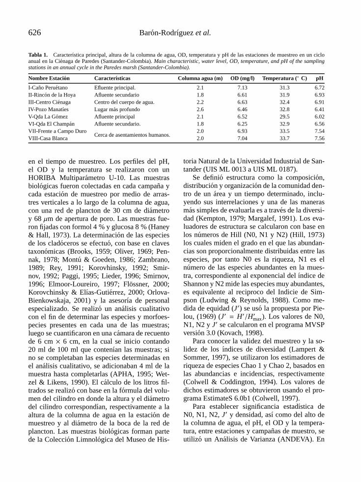
Los datos analizados fueron los obtenidos porGavilan-Dıaz (2000) en la Cienaga de Paredes enocho estaciones y en 11 campanas de muestreo(Febrero de 1998 a Enero de 1999). En la Tabla1 y en la figura 1 se muestra la distribucion delas estaciones en la cienaga y las caracterısticasfısicas y quımicas mas importantes de la cienaga
626 Baron-Rodrıguez et al.
Tabla 1. Caracterıstica principal, altura de la columna de agua, OD, temperatura y pH de las estaciones de muestreo en un cicloanual en la Cienaga de Paredes (Santander-Colombia). Main characteristic, water level, OD, temperature, and pH of the samplingstations in an annual cycle in the Paredes marsh (Santander-Colombia).
Nombre Estacion Caracterısticas Columna agua (m) OD (mg/l) Temperatura (◦ C) pH
I-Cano Peruetano Efluente principal. 2.1 7.13 31.3 6.72II-Rincon de la Hoya Afluente secundario 1.8 6.61 31.9 6.93III-Centro Cienaga Centro del cuerpo de agua. 2.2 6.63 32.4 6.91IV-Pozo Manatıes Lugar mas profundo 2.6 6.46 32.8 6.41V-Qda La Gomez Afluente principal 2.1 6.52 29.5 6.02VI-Qda El Champan Afluente secundario. 1.8 6.25 32.9 6.56VII-Frente a Campo Duro
Cerca de asentamientos humanos.2.0 6.93 33.5 7.54
VIII-Casa Blanca 2.0 7.04 33.7 7.56
en el tiempo de muestreo. Los perfiles del pH,el OD y la temperatura se realizaron con unHORIBA Multiparametro U-10. Las muestrasbiologicas fueron colectadas en cada campana ycada estacion de muestreo por medio de arras-tres verticales a lo largo de la columna de agua,con una red de plancton de 30 cm de diametroy 68 µm de apertura de poro. Las muestras fue-ron fijadas con formol 4 % y glucosa 8 % (Haney& Hall, 1973). La determinacion de las especiesde los cladoceros se efectuo, con base en clavestaxonomicas (Brooks, 1959; Oliver, 1969; Pen-nak, 1978; Montu & Goeden, 1986; Zambrano,1989; Rey, 1991; Korovhinsky, 1992; Smir-nov, 1992; Paggi, 1995; Lieder, 1996; Smirnov,1996; Elmoor-Loureiro, 1997; Flossner, 2000;Korovchinsky & Elıas-Gutierrez, 2000; Orlova-Bienkowskaja, 2001) y la asesorıa de personalespecializado. Se realizo un analisis cualitativocon el fin de determinar las especies y morfoes-pecies presentes en cada una de las muestras;luego se cuantificaron en una camara de recuentode 6 cm × 6 cm, en la cual se inicio contando20 ml de 100 ml que contenıan las muestras; sino se completaban las especies determinadas enel analisis cualitativo, se adicionaban 4 ml de lamuestra hasta completarlas (APHA, 1995; Wet-zel & Likens, 1990). El calculo de los litros fil-trados se realizo con base en la formula del volu-men del cilindro en donde la altura y el diametrodel cilindro correspondıan, respectivamente a laaltura de la columna de agua en la estacion demuestreo y al diametro de la boca de la red deplancton. Las muestras biologicas forman partede la Coleccion Limnologica del Museo de His-
toria Natural de la Universidad Industrial de San-tander (UIS ML 0013 a UIS ML 0187).
Se definio estructura como la composicion,distribucion y organizacion de la comunidad den-tro de un area y un tiempo determinado, inclu-yendo sus interrelaciones y una de las manerasmas simples de evaluarla es a traves de la diversi-dad (Kempton, 1979; Margalef, 1991). Los eva-luadores de estructura se calcularon con base enlos numeros de Hill (N0, N1 y N2) (Hill, 1973)los cuales miden el grado en el que las abundan-cias son proporcionalmente distribuidas entre lasespecies, por tanto N0 es la riqueza, N1 es elnumero de las especies abundantes en la mues-tra, correspondiente al exponencial del ındice deShannon y N2 mide las especies muy abundantes,es equivalente al reciproco del Indicie de Sim-pson (Ludwing & Reynolds, 1988). Como me-dida de equidad (J′) se uso la propuesta por Pie-lou, (1969) (J′ = H′/H′max). Los valores de N0,N1, N2 y J′ se calcularon en el programa MVSPversion 3.0 (Kovach, 1998).
Para conocer la validez del muestreo y la so-lidez de los ındices de diversidad (Lampert &Sommer, 1997), se utilizaron los estimadores deriqueza de especies Chao 1 y Chao 2, basados enlas abundancias e incidencias, respectivamente(Colwell & Coddington, 1994). Los valores dedichos estimadores se obtuvieron usando el pro-grama EstimateS 6.0b1 (Colwell, 1997).
Para establecer significancia estadıstica deN0, N1, N2, J′ y densidad, ası como del alto dela columna de agua, el pH, el OD y la tempera-tura, entre estaciones y campanas de muestro, seutilizo un Analisis de Varianza (ANDEVA). En

Cladoceros de la cienaga de Paredes (Santander, Colombia) 627
Figura 2. Variacion de la densidad numerica total de Cladocera y de las especies mas abundantes en: a) Campanas muestreo yb) Estaciones de muestreo. Variation of the total numeric density of Cladocera and the most abundant species in: a) Field trips, b)Sampling stations.
caso de obtener diferencias significativas, se uti-lizo la prueba a posteriori de Scheffe. Para estosanalisis se empleo el programa Statistica v 5.1(Statsoft, 1996).
RESULTADOSSe encontraron 19 especies y 12 morfoespecies,pertenecientes a dos ordenes y siete familias (Ta-bla 2). Del total de las especies y las morfoes-pecies encontradas, las mas abundantes represen-
tan el 81.9 % (Moina minuta, 49.2 %; Diapha-nosoma brevireme, 17.2 %; Ceriodaphnia cor-nuta, 9.3 % y Moina cf. micrura, 6.2 %); las es-pecies y morfoespecies restantes representan el18.1 %. La variacion de la abundancia relativa delas especies y morfoespecies dominantes en lascampanas y estaciones de muestreo, se puede ob-servar en las figuras 2a y 2b, en las que se veque el mayor porcentaje lo presenta M. minuta,con excepcion de las campanas de muestreo demarzo, octubre y principios de noviembre y las

628 Baron-Rodrıguez et al.
estaciones V y VI en las que predominaron las es-pecies D. brevireme, C. cornuta y M.cf. micrura.
Durante las campanas de muestreo los valo-res maximos densidad numerica se presentaron,en marzo y en septiembre, con valores de 5373ind/m3 y 5318 ind/m3 respectivamente, y valoresmınimos en julio, agosto y diciembre (Fig. 3a).En cuanto a las estaciones de muestreo loscladoceros alcanzaron su maxima densidad nu-merica en la EIII, con 5822 ind/m3 y mınima en laestacion V con 339 ind/m3 (Fig. 3b). El valor me-dio de la densidad fue 3491 ind/m3, con un maxi-mo de 12636 ind/m3 y un mınimo de 22 ind/m3.
De las 31 especies y morfoespecies observa-
das, los estimadores Chao 1 y 2 (Fig. 4a) infie-ren que no se incrementara este numero en lacienaga si se aumentara el esfuerzo de muestreocon las tecnicas utilizadas. El comportamiento delos unicos, singletones, duplicados y dobletones(Fig. 4b) revelo que el muestreo fue suficiente(Colwell & Coddington, 1994). Por lo tanto, laequidad y los numeros de Hill evaluados, estanbasados en muestreos efectivos.
Los evaluadores numericos de estructura (J′,N0, N1, N2), la abundancia de cladoceros y el pHpresentaron diferencias significativas entre esta-ciones de muestreo (Scheffe, p = 0.000 a 0.001);dichas diferencias fueron entre la estacion V y el
Figura 3. Cambios de la densidad numerica de Cladocera en: a) Campanas muestreo y b) Estaciones de muestreo. Changes in thenumeric density of Cladocera in: a) Field trips, b) Sampling stations.

Cladoceros de la cienaga de Paredes (Santander, Colombia) 629
Tabla 2. Composicion de Cladocera, en la Cienaga de Pa-redes (Santander-Colombia). Composition of Cladocera in theCienaga de Paredes (Santander-Colombia).
ORDEN CTENOMOPODAFAMILIA SIDIDAE Diaphanosoma spinulosum
Diaphanosoma dentatumDiaphanosoma breviremeLatonopsis spSarcilatona serricaudaPseudosida bidentata
ORDEN ANOMOPODAFAMILIA DAPHNIDAE Ceriodaphnia cornuta
Simocephalus latirostrisScapholeberis armata
FAMILIA MOINIDAE Moina minutaMoina cf. micruraMoinodaphnia macleayii
FAMILIA BOSMINIDAE Bosmina hagmanniBosmina tubicenBosminopsis deitersi
FAMILIA MACROTRICIDAE Macrothrix spGrimaldina brazzai
FAMILIA ILYOCRYPTIDAE Ilyocryptus spiniferFAMILIA CHYDORIDAESUBFAMILIA CHYDORINAE Ephemeroporus tridentatus
Dadaya macropsSUBFAMILIA ALONINAE Leydigia cf. striata
Alonella cf. dadayiAlonella spKurzia latissimaGraptoleberis testudinariaCamptocercus spNotoalona spAlona sp1Alona sp2Alona sp3Alona sp4
resto de estaciones (Scheffe, p = 0.000 − 0.034).El alto de la columna de agua, el OD y latemperatura no presentaron diferencias signifi-cativas espaciales ( p = 0.666 a 0.999). En-tre campanas de muestreo se presentaron di-ferencias significativas en la equidad, la ri-queza, en el alto de la columna de agua, elOD, la temperatura y el pH, presentando di-ferencias entre campanas para las tres ultimas(Scheffe, p = 0.000), ya que para la equidad se en-contraron diferencias entre las campanas de abrily finales de noviembre (Scheffe, p = 0.035).
La riqueza temporal, presento valores ma-ximos en las campanas de abril y de enero ymınimos en la de diciembre (Fig. 5a). En cuanto
a las estaciones, la mayor riqueza se encontro enla estacion V y el menor en la estacion VIII (Fig.5b). Los numeros de Hill N1 (especies abundan-tes) y N2 (especies muy abundantes), presentaronuna tendencia similar a lo largo de las estacionesy campanas de muestreo (Figs. 6a y 6b), con va-lores maximos en las campanas de octubre y definales de noviembre y mınimos en la campanade agosto. Los valores maximos de N1 y N2 sepresentaron en la estacion V. Los mayores va-lores de equidad, se presentaron en la campanade finales de noviembre (0.71) y en la estacionV (0.77) y los menores valores de equidad en la
Figura 4. Curvas de acumulacion de especies y morfoespe-cies: a) Estimadores Chao 1, Chao 2 y morfoespecies obser-vadas (Sobs), b) unicos, duplicados, singletones y dobletonesde Cladocera. Cummulative curves for species and morphospe-cies: a) Esimators Chao 1, Chao2, and observed morphospe-cies (Sobs), b) unique, duplicates, singletons and doubletons ofCladocera.
630 Baron-Rodrıguez et al.
campana de abril (0.34) y en todas las estacio-nes a excepcion de la estacion V (0.57 a 0.45).
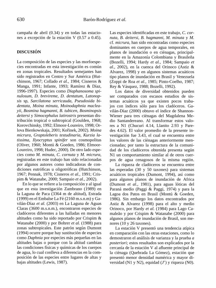
DISCUSION
La composicion de las especies y las morfoespe-cies encontradas en esta investigacion es comunen zonas tropicales. Resultados semejantes hansido registrados en Centro y Sur America (Hut-chinson, 1967; Collado et al., 1984; Cisneros &Manga, 1991; Infante, 1993; Ramırez & Dıaz,1996-1997). Especies como Diaphanosoma spi-nulosum, D. brevireme, D. dentatum, Latonop-sis sp, Sarcilatona serricauda, Pseudosida bi-dentata, Moina minuta, Moinodaphnia maclea-yii, Bosmina hagmanni, B. tubicen, Bosminopsisdeitersi y Simocephalus latirostris presentan dis-tribucion tropical o subtropical (Goulden, 1968;Korovchinsky, 1992; Elmoor-Loureiro, 1998; Or-lova Bienkowskaja, 2001; Korinek, 2002). Moinamicrura, Graptoleberis testudinaria, Kurzia la-tissima, Ilyocryptus spinifer son cosmopolitas(Oliver, 1960; Montu & Goeden, 1986; Elmoor-Loureiro, 1998; Hudec, 2000). De otro lado espe-cies como M. minuta, C. cornuta y M. micrura,registradas en este trabajo han sido relacionadaspor algunos autores como indicadoras de con-diciones eutroficas u oligotroficas (Hutchinson,1967; Pennak, 1978; Cisneros et al., 1991; Cris-pim & Watanabe, 2000; Sampaio et al., 2002).
En lo que se refiere a la composicion y al igualque en esta investigacion Zambrano (1989) enla Laguna de Paca (3364 m de altitud), Estrada(1999) en el Embalse La Fe (2160 m.s.n.m) y Ga-vilan-Dıaz et al. (2003) en La Laguna de AguasClaras (3600 m.s.n.m.), encontraron especies decladoceros diferentes a las halladas en menoresaltitudes como ha sido reportado por Crispim &Watanabe (2000) y por Bohrer et al. (1988) parazonas subtropicales. Este patron segun Dumont(1994) ocurre porque hay sustitucion de especiescomo Daphnia por especies mas pequenas en lasaltitudes bajas o porque con la altitud cambianlas condiciones fısicas y quımicas de los cuerposde agua, lo cual conlleva a diferencias en la com-posicion de las especies entre lugares de altas ybajas altitudes (Lewis, 1987).
Las especies identificadas en este trabajo, C. cor-nuta, B. deitersi, B. hagmanni, M. minuta y M.cf. micrura, han sido encontradas como especiesdominantes en cuerpos de agua temporales, enplanos de inundacion o en cienagas, principal-mente en la Amazonıa Colombiana y Brasilena(Bozelli, 1994; Hardy et al., 1984; Sampaio etal., 2002), en la cuenca del Orinoco (Astiz &Alvarez, 1998) y en algunos sistemas acuaticostipo planos de inundacion en Brasil y Venezuela(Zoppi de Roa et al., 1985; Pinto-Coelho, 1987;Rey & Vasquez, 1988; Bozelli, 1992).
Los datos de diversidad obtenidos puedenser comparados con escasos estudios de sis-temas acuaticos ya que existen pocos traba-jos con ındices solo para los cladoceros. Ga-vilan-Dıaz (2000) obtuvo el ındice de Shannon-Wiener para tres cienagas del Magdalena Me-dio Santandereano. Al transformar estos valo-res a N1 (Chucurı 4.14, Llanito 2.93 y Pare-des 4.62). El valor promedio de la presente in-vestigacion fue 3.43, el cual se encuentra entrelos valores de las cienagas anteriormente men-cionadas; por tanto la estructura de la comuni-dad de los cladoceros obtenida presenta segunN1 un comportamiento similar al de otros cuer-pos de agua cenagosos de la misma region.
La riqueza de cladoceros se encuentra entrelas esperadas (30 y 50 taxones) para sistemasacuaticos tropicales (Dumont, 1994), ası comopara algunos planos de inundacion de Africa(Dumont et al., 1981), para aguas loticas delParana medio (Paggi & Paggi, 1974) y para laLagoa dos Patos en Brasil (Montu & Goeden,1986). Sin embargo los datos encontrados porAstiz & Alvarez (1998) para el alto y medioOrinoco, por Hardy et al. (1984) para Lago Ca-maleao y por Crispim & Watanabe (2000) paraalgunos planos de inundacion de Brasil, son me-nores (10 y 26 taxones).
La estacion V presento una tendencia atıpicaen comparacion con las otras estaciones, como lodemostraron el analisis de varianza y la prueba aposteriori; estos resultados son explicados por lacercanıa de la estacion V al afluente principal dela cienaga (Quebrada La Gomez), estacion quepresento menor densidad numerica y mayor di-versidad (N1 y N2), equidad (J′) y riqueza (N0).

Cladoceros de la cienaga de Paredes (Santander, Colombia) 631
Figura 5. Dinamica de la riqueza de Cladocera en un ciclo anual en la Cienaga de Paredes en: a) Campanas de muestreo, b)Estaciones de muestro. Cladocera richness dynamics in an annual cycle in the Cienaga de Paredes in: a) Field trips, b) Samplingstations.
Hecho que no puede ser atribuido a la variacionde la columna del agua ya que esta no presentodiferencias significativas entre las estaciones demuestreo, ni a la presencia de macrofitas flotan-tes ya que estas se presentaron en las tres ultimascampanas de muestreo en toda la cienaga.
La tendencia atıpica de la estructura de la co-munidad de los cladoceros en la estacion V esatribuido segun lo encontrado en este estudio a:1) las diferencias de pH entre la estacion V y elresto de las estaciones, ya que el pH es una va-riable para la cual las poblaciones de cladocerospresentan estrechos niveles de tolerancia para su
desarrollo (Lampert & Sommer, 1997); y 2) a quelugares expuestos a perturbaciones frecuentes yde magnitud moderada Connell (1978), en estecaso el movimiento y la fluctuacion de nutrientesdebidas a las corrientes, presentan mayor diversi-dad. Thompson & Townsend (2000), lo explicandiciendo que las perturbaciones de las comuni-dades en arroyos pueden deberse a variacion enel caudal. Adicionalmente es importante resal-tar lo encontrado por Montenegro (1995) quienestudio varias estaciones de muestreo entre lasque se encontraban lugares cercanos a la desem-bocadura de la Quebrada La Gomez (estacion

632 Baron-Rodrıguez et al.
Figura 6. Variacion de los numeros de Hill N1 y N2 en: a) Campanas muestreo, b) Estaciones de muestro. Variation of the HillNumbers N1 and N2 in: a) Field trips, b) Sampling stations.
V); esta estacion se caracterizo por la presenciade macrofitas sumergidas, menor densidad fito-planctonica y menor densidad de cladoceros ycopepodos, lo cual concuerda con lo hallado enesta investigacion e indica la existencia de pocoalimento disponible en este lugar.
Adicionalmente, las diferencias en la abun-dancia de cladoceros entre estaciones indican quelas condiciones en la estacion V no favorecendensidades mayores a las halladas en este trabajo.Baron-Rodrıguez et al. (2005), al aplicar un PCAen esta Cienaga en el mismo periodo de estudioencontraron que para todos los puntos de mues-treo excepto para la estacion V, la abundancia decladoceros estuvo relacionada positivamente con
el pH, la turbidez, la temperatura del agua y la he-terogeneidad de la columna para estas variables,mientras que la relacion con la transparencia fuenegativa. La referencia anterior verifica los resul-tados del analisis en este ıtem.
La variacion temporal de la estructura se re-fleja en las diferencias significativas encontradasen la equidad y la riqueza entre las campanasde muestreo a traves del ciclo. El hecho de noencontrar las mismas especies y morfoespeciesdominantes indica que temporalmente hubosustitucion de especies y por lo tanto cambioen sus respectivas densidades numericas. Estosresultados son consecuencia de los cambiostemporales en las condiciones fısicas y quımicas

Cladoceros de la cienaga de Paredes (Santander, Colombia) 633
del sistema debidas al regimen climatico.Baron-Rodrıguez et al. (2005), describen larelacion positiva entre la precipitacion, el niveldel agua y la transparencia con las variablesbioticas equidad y diversidad, y la relacionnegativa entre estas y la turbidez, los nutrientes,el pH, la conductividad y la densidad numerica.Este analisis permite establecer que existenlas condiciones adecuadas para el desarrollo ytemporalidad de la comunidad de cladoceros.
Se concluye entonces que en cuanto a la va-riacion espacial de la estructura la estacion Vpresento condiciones que ocasionaron una dis-minucion en la densidad numerica, aumento dela equidad, la riqueza y la diversidad, contextoque es explicado por las caracterısticas bioticasy abioticas del lugar y por la influencia de per-turbacion de caracter intermedio. La variaciontemporal de la estructura de la comunidad decladoceros se debio a las fluctuaciones en la equi-dad, la riqueza y el cambio de la abundancia re-lativa de las morfoespecies; lo anterior, debido ala influencia de la variacion de la precipitacion yde la columna de agua en el sistema acuatico enestudio. En general la estructura de la comunidadde cladoceros presente en la cienaga de Paredesmostro heterogeneidad espacial y temporal.
AGRADECIMIENTOS
Los autores agradecen a las profesoras LourdesMarıa Elmoor Loureiro (Universidade Catolicade Brasilia), Odete Rocha (Universidad Federalde Sao Carlos –Brasil), Evelyn Zoppi de Roa(Universidad Central de Venezuela) y MarinaManca (Istituto per lo Studio degli Ecosistemi-CNR), por confirmar las especies encontradas.
BIBLIOGRAFIA
AMERICAN PUBLIC HEALTH ASSOCIATION.(APHA). 1995. Standard Methods for the Exami-nation of Water and Wastewater. 19th ed. Washing-ton. 874 pp.
ARIAS, P. 1985. Las Cienagas de Colombia. RevistaDivulg. Pesq. Inderena, 22: 39-70.
ASTIZ, S. & H. ALVAREZ. 1998. El zooplanctonen el alto y medio Rıo Orinoco, Venezuela. ActaCientıfica Venezolana, 49: 5-18.
BARON-RODRIGUEZ M. M., R. A. GAVILAN-DIAZ & J. J. RAMIREZ. 2005. Factor and varia-bles related to the temporl and spatial fluctuationof the numeric density of Cladocera in a lowlandneotropical cienaga. VIIth International Sympo-sium on Cladocera. September 3-9, 2005, Herz-berg. Switzerland.
BOHRER, M. B. C., M. M. ROCHA & B. F. GO-DOLPHIM. 1988. Variacoes espaco-temporais daspopulacoes de Cladocera (Crustacea-Branchiopo-da) no Saco de Tapes, Laguna Dos Patos, R.S. ActaLimnol. Brasil., 11: 549-570.
BOZELLI, R. L. 1992. Composition of the zooplank-ton community of Batata and Mussura Lakes andof the Trombetas River, State of Para, Brazil. Ama-zoniana, XII (2): 239-261.
BOZELLI, R. L. 1994. Zooplankton communitydensity in relation to water level fluctuationsand inorganic turbity in an Amazonian lake,“Lago Batata”, State of Para, Brazil. Amazoniana,XIII(1/2): 17-32.
BROOKS, J. L. 1959. Cladocera. In: Fresh-WaterBiology. W. T. Edmonson (ed): 587-656. 2ond ed.John Willey & Sons, INC. USA.
CISNEROS, R. & E. I. MANGA. 1991. Zooplank-ton studies in a tropical lake (Lake Xolotlan, Nica-ragua). Verh. Internat. Verein. Limnol., 24: 1167-1170.
CISNEROS, R., E. I. MANGA & M. VAN MAREN.1991. Qualitative and quantitative structure, diver-sity and fluctuations in abundance of zooplanktonin a lake Xolotlan (Managua). Hydrobiol. Bull.,25(2): 151-156.
COLLADO, C., C. H. FERNANDO & D. SEPH-TON. 1984. The freshwater zooplankton of Cen-tral America and the Caribbean. Hidrobiologia,113: 105-119.
COLWELL, R. K., & J. A. CODDINGTON. 1994.Estimating terrestrial biodiversity through extrapo-lation. Phil. Trans. Royal Soc., (Series B) 345: 101-118.
COLWELL, R. K. 1997. EstimateS: statistical esti-mation of species richness and shared species fromsamples. Version 6.01b. User’s Guide and appli-cation published at: http://viceroy.eeb.uconn.edu/estimates
CONNELL, J. H. 1978. Diversity in tropical rain fo-rest and coral reefs. Science, 199: 1302-1310.

634 Baron-Rodrıguez et al.
CORMAGDALENA, 1999. Rıo Magdalena. Visitatecnica Cienagas de Paredes, El Llanito y Chucurı(Santander). IGAC. 12 pp.
CRISPIM, M. C. & T. WATANABE. 2000. Caracte-rizacao Limnologica das bacias doadoras o recep-toras de aguas do Rio Sao Francisco: 1-Zooplanc-ton. Acta. Limnol. Bras., 12: 93-103.
DUMONT, H. J., J. PENSAERT & I. V. DE VELDE.1981. The crustacean zooplankton of Mali (WestAfrica). Hydrobiologia, 80: 161-187.
DUMONT, H. J. 1994. On the diversity of the Clado-cera in the tropics. Hydrobiologia, 272: 29-38.
ELMOOR-LOUREIRO, L. M. A. 1997. Manual deidentificacao de Cladoceros lımnicos do Brasil.Editora Universa. Universidad Catolica de Brasi-lia. Brasil. 155 pp.
ELMOOR-LOUREIRO, L. M. A. 1998. Branchio-poda Freshwater Cladocera. In: Cataloque ofCrustacea of Brazil. P. S. Young (ed.): 15-41. Riode Janeiro: Museu Nacional.
ESTRADA, A. L. 1999. Variacao espacial e tempo-ral da comunidade zooplanctonica do reservatorioLa Fe, Antioquia, Colombia. Tese grado, Universi-dade de Sao Paulo. 130 pp.
FERNANDO, C. H., C. TUDORANCEA & S.MENGESTOU. 1990. Invertebrate zooplanktonpredator composition and diversity in tropicallentic waters. Hidrobiologia, 198: 13-31.
FLOSSNER, D. 2000. Die Haplopoda und Clado-cera (ohne Bosminidae) Mitteleuropas. BackhuysPublishers, Leiden, The Netherlands. 428 pp.
GARCIA, L. & E. DISTER. 1990. La planicie deinundacion del medio-bajo magdalena: restau-racion y conservacion de habitats. Interciencia, 15:396-410.
GAVILAN-DIAZ, R. A. 2000. Analisis de la diver-sidad en cienagas del Magdalena Medio Santan-dereano (Neotropico) con enfasis en la Comuni-dad zooplanctonica y el ciclo hidrologico regional.Fase I y II. Informe Convenio UIS-Cormagdalena.353 pp.
GAVILAN-DIAZ, R. A., Y. PLATA-DIAZ & M. M.BARON-RODRIGUEZ. 2003. Plancton de unlago de Alta Montana neotropical (Aguas Claras-Santander-Colombia). Informe Final del contratode investigacion 319-2000. Colciencias –UIS–Grupo de Estudios en Biodiversidad. 58-84 pp.
GOULDEN, C. E. 1968. The systematics and evolu-tion of the Moinidae. Trans. Am. Phil. Soc., 58: 1-101.
HANEY, J. F. & D. J. HALL. 1973. Sugar-coatedDaphnia: a preservation technique for Cladocera.Limnol. Oceanogr., 18: 331-339.
HARDY, E. R., B. ROBERTSON & W. KOSTE.1984. About the relationship between the zoo-plankton and fluctuating water levels of Lago Ca-maleao, a Central Amazonian varzea lake. Amazo-niana, IX: 43-52.
HILL, N. O. 1973. Diversity and evenness: A unif-ying notation and its consequences. Ecology, 54:427-432.
HOLDRIDGE, R. 2000. Ecologıa basada en zonasde vida. Instituto Interamericano de Cooperacionpara la Agricultura. IICA, San Jose de Costa Rica.216 pp.
HUDEC, I. 2000. Subgeneric differentiation withinKurzia (Crustacea: Anomopoda: Chydoridae) anda new species from Central America. Hydrobiolo-gia, 421: 165-178.
HUTCHINSON, G. E. 1967. A treatise of Limno-logy. John Willey & Sons, INC. New York. 1115pp.
INFANTE, A. G. 1993. Vertical and horizontal distri-bution of the zooplankton in a lake Valencia. Acta.Limnol. Bras., VI: 97-105.
JUNK, W., P. B. BAYLEY & R. E. SPARKS. 1989.The flood pulse concept in river-floodplain sys-tems. Can. Spec. Publ. Fish. Aquat. Sci., 106: 110-127.
JUNK, W. J. 1996. Ecology of floodplains –a cha-llenge for tropical limnology. In: Perspectives intropical limnology. F. Shiemer & K. T. Boland(eds.): 255-265. SPB Academic Publishing, Ams-derdam.
KEMPTON, R. A. 1979. The structure of speciesabundance and measurement of diversity. Biome-trics, 35:307-321.
KOIINEK, V. 2002. Cladocera. In: A Guide to Tropi-cal Freshwater Zooplankton. C. H. Fernando (ed.):69-122. Backhuys Publishers, Leiden, The Nether-lands.
KOROVCHINSKY, N. M. 1992. Guides to the Iden-tification of the Microinvertebrates of the Conti-nental Waters of the World N◦ 3. Sididae & Ho-lopodidae. (Crustacea: Daphniiformes). SPB Aca-demic Publishing, The Netherlands. 86 pp.
KOROVCHINSKY, N. M. & M. ELIAS-GUTIE-RREZ. 2000. First record of Sarcilatona serri-cauda (Sars, 1901) (Crustacea: Branchiopoda:Sididae) from Mexico, with redescription of itsmale. Arthropoda Selecta., 9(1): 5-11.

Cladoceros de la cienaga de Paredes (Santander, Colombia) 635
KOVACH, W. 1998. MVSP v 3.00b for Windows.Multivariate Statistical Package. UK.
LAMPERT, W. & U. SOMMER 1997. Limnoeco-logy. The ecology of lakes and streams. OxfordUniversity Press. New York. 382 pp.
LANSAC TOHA, F. A., A. F. LIMA, S. M. THO-MAZ & M. C. ROBERTO. 1993. Zooplanctonde uma planicie de inundacao do Rio Parana.II. Variacao sazonal e influencia dos nıveis flu-viometricos sobre a comunidade. Acta Limnolo-gica Braziliensia, (VI): 42-55.
LEWIS, W. 1987. Tropical Limnology. Ann. Rev.Ecol. Syst., 18: 159-184.
LIEDER, V. U. 1996. Crustacea. Cladocera/Bosmi-nidae. Gstav Fischer, Berlin. 84 pp.
LUDWING, J. A. & REYNOLDS, J. F. 1988. Statis-tical ecology. A primer on methods and computing.John Wiley & Sons. New Cork. 337 pp.
MARGALEF, R. 1991. Ecologıa. Ed. Omega. Barce-lona. 951 pp.
MONTENEGRO, M. I. 1995. Evaluacion ambientalde la Cienaga de Paredes. Sabana de Torres, San-tander, como habitat para fauna silverstre; conespecial enfasis en el Manatı (Trichechus mana-tus) –Primera fase. Informe Division de FaunaTerrestre– INDERENA & Fundacion para la Pro-mocion de la Investigacion y la Tecnologıa Bancode la Republica. 81 pp.
MONTU, M. & I. M. GOEDEN. 1986. Atlas dosCladocera e Copepoda (Crustacea) do Estuario daLagoa Dos Patos (Rio Grande, Brasil). Neritica,1(2): 1-134.
OLIVER, S. 1969. Los Cladoceros Argentinos conclaves de las especies, notas biologicas y distri-bucion geografica. Revista del Museo de la Plata,7: 173-269.
ORLOVA-BIENKOWSKAJA, M. Y. 2001. Guidesto the Identification of the Microinvertebratesof the Continental Waters of the World N◦ 17.Cladocera: Anomopoda. Daphniidae: genusSimocephalus. Backhuys Publishers, Leiden. TheNetherlands. 128 pp.
PAGGI, C. P. & S. J. PAGGI. 1974. Primeros estu-dios sobre el zooplancton de aguas loticas del Pa-rana medio. Physis, 33(86): 91-114.
PAGGI, J. C. 1995. Crustacea Cladocera. En: Ecosis-temas de Aguas Continentales. E. C. Lopretto y G.Tell (eds): 909-951. Tomo III. Ediciones Sur. Ar-gentina.
PENNAK, R. W. 1978. Fresh-Water Invertebrates ofthe United States. Wiley. USA. 798 pp.
PIELOU, E. C. 1969. Ecological Diversity and ItsMeasurement. In: An Introduction to Mathemati-cal Ecology. E. C. Pielou (ed.): 221-235. John Wi-ley & Sons. United States of America.
PINTO-COELHO, R. M. 1987. Fluctuacoes sazonaise de curto duracao na comunidade zooplanctonicado Lago Paranoa, Brasilia-D.F. Brasil. Rev. Brasil.Biol., 47: 17-29.
RAMIREZ. J. J. & A. DIAZ. 1996-1997. Fluc-tuacion estacional del zooplancton en la lagunadel Parque Norte, Medellın, Colombia. Rev. Biol.Trop., 44/45: 549-563.
REY, J. & E. VASQUEZ. 1988. Notas sobre losavances de las investigaciones de los cladoceros(Crustacea, Cladocera) de la Cuenca baja del Ori-noco. Sociedad de ciencias Naturales La Salle,XLVIII: 155-161.
REY, J. 1991. Los Cladoceros. En: El Lago Titicaca:sıntesis del conocimiento limnologico actual. De-joux C. y A. Iltis (eds.): 265-276. ORSTOM. Boli-via.
ROESSLER, E. W. 1994. Los cladoceros de la fami-lia Sididae Baird, 1850, en Colombia. (Crustacea,Cladocera). Comite de investigaciones, Universi-dad de los Andes, Bogota, D. E., Colombia. 27 pp.
ROESSLER, E. W. 1996. La familia Moinidae enColombia. (Arthropoda, Crustacea, Cladocera).Los Moinidae de la amazonıa colombiana. Comitede investigaciones, Universidad de los Andes, Bo-gota, D. E., Colombia. 25 pp.
SAMPAIO, E., O. ROCHA, T. MATSUMURA-TUNDISI & J. G.TUNDISI. 2002. Compositionand abundance of zooplankton in the limneticzone of seven reservoirs of the ParanapanemaRiver, Brazil. Braz. J. Biol., 62: 525-545.
SENDACZ. S., E. KUBO & L. P. FUJIARA. 1984.Further studies on the zooplankton community ofa eutrophic reservoir in southern Brazil. Verh. In-ternt. Verein. Limnol., 22: 1625-1630.
SENDACZ, S. & E. KUBO. 1999. Zooplancton dereservatorios do Alto Tiete. In: Ecologia de re-servatorios: estructura, funcao e aspectos sociais.R. Henry (ed.): 509-530. Botucatu, FUNDIO-BIO/FAPESP.
SMIRNOV, N. N. 1992. Guides to the Identificationof the Microinvertebrates of the Continental Wa-ters of the World N◦ 1. The Macrothricidae ofthe World. SPB Academic Publishing, The Nether-lands. 150 pp.

636 Baron-Rodrıguez et al.
SMIRNOV, N. N. 1996. Guides to the Identificationof the Microinvertebrates of the Continental Wa-ters of the World N◦ 11. Cladocera: the Chydori-nae and Sayciinae (Chydoridae) of the World. SPBAcademic Publishing, The Netherlands. 248 pp.
STATSOFT, INC., 1996. Statistica v 5.1 for Windows[Computer program manual]. Tulsa.
THOMPSON, R. M. & C. M. TOWNSEND. 2000.New Zealand’s Stream Invertebrate Communities:An International Perspective. In: New Zealandstream invertebrates: ecology and implications formanagement. K. J. Collier & M. J. Winterbourn(eds.): 53-74. New Zealand Limnological Society,Christchurch.
VALDIVIA, R. 1988. Lista de Cladoceros dul-ceacuıcolas del Peru. Amazoniana, X(3): 283-297.
WETZEL, R. G. & G. E. LIKENS. 1990. Limnologi-cal Analyses. W. B. Saunders Company. USA. 391pp.
ZAMBRANO, F. 1989. Estudio taxonomico de loscladoceros de la Laguna de Paca (Jauja-Junın).Tesis de Grado. Facultad de Ciencias Biologicas.Universidad Ricardo Palma. 141 pp.
ZOPPI DE ROA, E., F. MICHELANGELLI. & L.SEGOVIA. 1985. Cladocera (Crustacea, Bran-chiopoda) de sabanas inundables de Mancal, Es-tado Apure, Venezuela. Acta Biol. Venez., 12: 43-55.

Limnetica, 25 (3-4): xx-xx (2006)Limnetica, 25 (3): 637-646 (2006)c© Asociacion Espanola de Limnologıa, Madrid. Spain. ISSN: 0213-8409
Influence of filtration and glucose amendment on bacterial growth rateat different tidal conditions in the Minho Estuary River (NW Portugal)
I. Anne1,2, M. L. Fidalgo1,2,∗, L. Thosthrup3 and K. Christoffersen3
(1) Department of Zoology and Anthropology, Faculty of Sciences, University of Porto, Praca Gomes Teixeira,4099-002 Porto, Portugal(2) Centre for Marine and Environmental Research (CIIMAR), Rua dos Bragas 289, 4050-123 Porto, Portugal(3) Freshwater Biological Laboratory, University of Copenhagen, Helsingørgade 51, DK-3400 Hillerød, Denmark(3) Freshwater∗ Corresponding author: [email protected]
ABSTRACT
Influence of filtration and glucose amendment on bacterial growth rate at different tidal conditions in the MinhoEstuary River (NW Portugal)
Bacterioplankton abundance, biomass and growth rates were studied in the Minho Estuary River (NW Portugal). The influenceof tidal conditions, glucose amendment, and the filtration process on total bacterial abundance, total and faecal coliforms, aswell as faecal streptococci, were evaluated in laboratory incubation experiments. Physical and chemical conditions, as well asbacterial abundance in this estuary were found to be typical for oligo-mesotrophic coastal ecosystems. Bacterial abundancewas higher at high tide, probably due to hydrodynamics and resuspension of bacteria from sediments. In contrast, a significantdecrease of bacterial indicators of faecal pollution at high tide was probably the result of various causes, such as the decreaseof continental and agricultural land run-off effect by dilution, and/or increase in the abundance of potential specific predators.Thus, drastic changes were induced at high tide that led to a lack of bacterial growth and the net disappearance of most of thebacterial populations. Glucose amendment, at used concentration, was not found to stimulate bacterial growth, which insteadcould be limited by inorganic nutrients.
Key words: Bacterioplankton, faecal indicators, filtration, glucose amendment, tides.
RESUMEN
Influencia de la filtracion y de la adicion de glucosa en la tasa de crecimiento bacteriano en diferentes condiciones demarea en el estuario del rıo Mino (Noroeste de Portugal)
La abundancia, la biomasa y las tasas de crecimiento de bacterioplancton fueron estudiadas en el estuario del rıo Mino(NW Portugal). La influencia de condiciones de marea, de la adicion de glucosa y del proceso de filtracion en la abundanciatotal de bacterias, coliformes totales y coliformes fecales, ası como de estreptococos fecales, fue evaluada en experimentosde incubacion en laboratorio. Las condiciones fısicas y quımicas, ası como la abundancia bacteriana encontradas en esteestuario son tıpicas para los ecosistemas costeros oligo-mesotroficos. La abundancia bacteriana fue mas alta en la alta marea,probablemente debido a la hidrodinamica y a la resuspension de bacterias de los sedimentos. En contraste, la disminucionsignificativa de los indicadores bacterianos de la contaminacion fecal en la alta marea resulto probablemente de variascausas, tales como la disminucion del efecto de vertido de la region continental y agrıcola por la dilucion, y/o aumento enla abundancia de depredadores especıficos potenciales. En resultado, cambios drasticos fueron inducidos en la alta mareaoriginando la ausencia de crecimiento bacteriano y la desaparicion neta de la mayorıa de las poblaciones bacterianas.La adicion de la glucosa, en la concentracion usada, no estimulo el crecimiento bacteriano, que se podrıa limitar por losalimentos inorganicos.
Palabras clave: Bacterioplancton, indicadores fecales, filtracion, adicion de glucosa, mareas.

638 Anne et al.
INTRODUCTION
Several environmental factors, such as predation,organic dissolved substrates, toxic compounds,temperature, and solar radiation may influencebacterial growth and survival in the aquaticenvironment (Sherr et al., 1989; Nybroe et al.,1992; Christoffersen et al., 1995; Hansen &Christoffersen, 1995; Suzuki, 1999; Caron et al.,2000; Calbet et al., 2001).
In estuarine areas, tides are natural pheno-mena that cause changes in the densities ofbacterial populations and heterotrophic activities(Cunha et al., 2000; 2001). The diversity of thebacterial assemblages may also be affected by thetwice-daily rhythm of tides, because the two sys-tems (ocean and estuarine waters) differ in termsof growth conditions and carrying capacity. Onthe other hand, microbiological pollution repre-sents one of the most widespread impairmentsfor water uses caused by urban drainage dischar-ges. Moreover, concerns about the spreading ofwaterborne diseases caused by such waters ledto the promulgation of bacteriological water qua-lity criteria which specify the tolerable concen-trations of various faecal indicator microorga-nisms. The primary criteria deals with indicatorbacteria (e.g. total coliforms, faecal coliforms,faecal streptococci, Escherichia coli) which indi-cate the potential presence of pathogens (USEPA,1986; Marsalek et al., 1994).
The study of the relationship between tideevents and faecal indicator bacteria in estua-rine areas is of great importance, because itallows making useful recommendations in termsof water use and public health protection (Fat-tal et al., 1986). In this sense, to know theestuarine dynamics of faecal indicator bacte-ria can represent an important contribution par-ticularly if effluent discharges reach estuarineareas as it occurs in the Minho Estuary Ri-ver. To our knowledge no previous studies werecarried out on this estuary concerning bacte-rial dynamics, which should encourage addi-tional investigations in order to fill this gap.
The main goals of this study were to deter-mine (i) the relationship between tidal eventsand abundance of faecal indicator bacteria in the
Minho Estuary River and (ii) the influence ofthe tidal conditions, filtration and glucose amend-ment on bacterial abundance and overall growthrate. Aiming to achieve the mentioned goals, afield-sampling programme was designed to cha-racterise the bacterioplankton pool in the Minhoestuary at low and high tides. Moreover, estua-rine water samples were experimentally manipu-lated in the laboratory to determine the overallgrowth rates of bacterioplankton assemblages.
Figure 1. Location of the sampling site in the MinhoEstuary River, North West coast of Portugal (Image fromthe National System of Geographic Information, Portugal).Ubicacion del punto de muestreo en el estuario del rıo Mino,costa Noroeste de Portugal. (Imagen del Sistema GeograficoNacional, Portugal).
MATERIAL AND METHODS
Sampling site
The Minho Estuary River is a temperatewater-body located in the North West coastof Portugal (41◦52′N, 08◦51′W) (Fig. 1). Thesampling site was established on the left bankof the Minho estuary, at the small town ofCaminha, approximately 1 km upstream of theAtlantic Ocean. Water samples were collectedin April 1998 (days 22 and 29) during the lowand high tide for the physical and chemicalcharacterisation of the estuarine water as wellas for the enumeration of bacterial abundance

Bacterial growth rate in the river Minho estuary 639
and faecal indicator bacteria; on days 22 and 29,water samples were experimentally manipulatedin the laboratory to determine the overall growthrate of bacterioplankton assemblages at low andhigh tide conditions, respectively.
Physical, chemical and bacteriologicalvariables
Water temperature, pH, dissolved oxygen, con-ductivity and salinity were determined in situusing an YSI Model 33 SCT meter and an YSIModel 54 oxygen probe.
Water samples from the bottom (about 1 mdepth and 3.5 m depth, at low and high ti-des, respectively) and from the water surface(about 0.1 m depth) were collected with a 2-liter Ruttner sampler and pooled into a com-posite sample of approximately 30 L. We keptcollected water samples in isolated isothermiccontainers which were transported to the labo-ratory within a few hours. In the laboratory, wehomogenised the water before we measured al-kalinity and chlorophyll a (Chl a). We measu-red alkalinity using the acidimetric indicator endpoint method (Golterman et al., 1978) and Chla according to Lorenzen (1967).
The total bacterial number (TBN) was de-termined by epifluorescence microscopy af-ter fixating water samples with glutaraldehyde(1.5 %, final concentration). The samples werefiltered through black Nuclepore filters (0.2µm pore size), stained with 4′, 6-diamidino-2-phenylindole (DAPI) (1µg/mL, final concentra-tion) according to Porter & Feig (1980); stainedfilters were mounted on glass slides with Leicaimmersion oil, and then frozen (−20◦ C) untilmicroscopic examination. On each filter, at least300 cells were counted in 10 fields (x1250 mag-nification) using a Leica DM LB 30T microscopeequipped with a fluorescence filter system (ultra-violet excitation filter of 340-380 nm, and emis-sion filter of 430 nm) and a fluotar 100/1.32 oilobjective. Cells were measured under an epifluo-rescent microscope with the aid of an ocular lensequipped with a reticule (Graticules Ltd).
The membrane filtration method included inthe APHA procedures (1992) and three dilutions
(sterile NaCl, 0.9 %) with three replicatesfor each dilution were used to count totalcoliforms (TC), faecal coliforms (FC), and faecalstreptococci (FS).
The specific growth rates of the bacterialassemblages in the laboratory experiments wereestimated as k = 1/t × ln (Nt/N0) (Mcmanus,1993), where k represents the growth rate, Nt thetotal bacterial number at time t, and N0 the totalbacterial number at time 0.
Determination of the total bacterial biomasswas based on a mean value of cell biovolume of0.07 µm3 that was obtained from size measure-ments of approximately 50 cells by each coun-ted field, and visualised on enlarged micrographs.The calculation was done according to the allo-metric relationship between cell volume and car-bon content reported by Norland (1993).
Experimental setup
For each tide condition, the experimental setupin the laboratory was as follows: a sub samplewas taken from the composite sample obtainedin the field and was distributed in twelve cleaned1.5 L polycarbonate bottles that were placedin a 15 L water bath. The water bath wascontinuously flooded with tap water to keep thesamples at 15-17◦ C, which was similar to thein situ temperature at the sampling time. Oneset of six bottles was filled with water screenedthrough a 20 µm mesh size net, while another setof six bottles was filled with water sequentiallyfiltered through GF/C filters and then through a1 µm pore size polycarbonate membrane filter.We assumed that the first set of bottles containedthe natural density of heterotrophic flagellatesand ciliates (<20 µm) and we also assumed thatthe second set did not contain the mentionedpredators. All bottles were incubated at roomlight and each bottle was aerated to create watercirculation by means of a tube connected to anair pump; a small piece of cotton was placed inthe free tip of the tube to avoid contaminationof the culture bottles by airborne bacteria. Thebottles were allowed to stand for 2 hours withoutfurther manipulation for acclimation before thefirst sampling. Then, three bottles of each set of

640 Anne et al.
six bottles were amended each with 1 mg glucoseper litre. Thus, each experimental condition wasrun three times.
The two experiments lasted four days, andsampling was performed every 24 hours, excepton the third day for the experiment at high tidecondition, because of logistical problems.
To compare the four sets of conditions foreach tide condition, we performed a statisticalanalysis day by day: we used the two-tailed t−testto test for differences between means of totalbacterial number and number of faecal indicatorbacteria at low and high tides; we assesseddifferences between the average biomass in alllaboratory treatments in each experiment by thenon-parametric Kruskal-Wallis ANOVA by ranks(Fowler et al., 1998).
RESULTS
Physical, chemical, and bacteriologicalvariables in the study site
The basic physical and chemical variablesmeasured in the sampled area are given in Table1. Water temperature varied between 12.4◦ C and13.3◦ C at low tide, and between 13.0◦ C and13.9◦ C at high tide. Estuarine waters were welloxygenated, and pH ranged from neutral (7.0) toslightly alkaline values (7.9). Measurements ofsalinity (0.0 and 0.3 �) and conductivity (120and 280 µS/cm) clearly reflected the dominanceof freshwater during low tide and that of marineoceanic water during high tide (23.0 � and29500 µS/cm). During high tide, salinity varied
Figure 2. Average field bacterial densities at low and hightides in the Minho Estuary River (Bar and whisker plot;bars: Mean ± Standard error; whiskers: Mean ± StandardDeviation; Total Bacterial Number: white rectangle; TotalColiforms: white circle; Faecal Coliforms: black square; FaecalStreptococci: cross). Densidades bacterianas promedio en bajay alta marea en el estuario del rıo Mino (Barras y figurawhisker; barras: Media ± Error estandar, whiskers: Media ±Desviacion estandar; Numero total de bacterias: rectanguloblanco; Coliformes totales: cırculo blanco; Coliformes fecales:cuadrado negro; Estreptococos fecales: cruz).
from 3.0 � at the water surface to 25.0 � at thebottom; conductivity varied from 5000 µS/cm(at water surface) to 31000 µS/cm (at thebottom), indicating the existence of a salinityand conductivity gradient in the prospected area.At low tide, there was practically no remainingsalinity and the conductivity was much lowercomparing with high tide.
This situation is typical for the Minho EstuaryRiver, because Azevedo (1995) reported similarvalues and confirms that our results were typicalfor that tidal influenced area. At high tide, alkali-nity was higher at both sampling dates, showing
Table 1. Physical and chemical variables of the pooled water samples (covering the entire vertical profile). Variables fısicas yquımicas promedio de las muestras de agua (agrupando a todo el perfil vertical).
Variables April 22, 1998 April 29, 1998
Low tide High tide Low tide High tide
Water temperature (◦ C) 13.3 13.0 12.4 13.9Dissolved oxygen (mg/L) 10.1 12.4 10.2 09.0pH 07.4 07.0 07.0 07.9Salinity (�) 00.0 23.0 00.3 23.0Conductivity (µS/cm) 120 29 500 280 29 500Alkalinity (mg CaCO3/L) 08.0 17.0 09.0 15.0Chlorophyll a (mg/m3) 01.6 00.8 01.3 01.3

Bacterial growth rate in the river Minho estuary 641
Figure 3. Temporal variation of total bacterial number and biomass in the low tide experiment (Bar and whisker plot; bars: Mean± Standard error; whiskers: Mean ± Standard Deviation; 20-µm screened sample: P; 1-µm filtered sample: NP; 20-µm screenedsample with glucose amendment: PG; 1-µm filtered sample with glucose amendment: NPG). Variacion temporal del numerototal de bacterias y biomassa durante el experimento en baja marea (Barras y figura whisker; barras: Media ± Error estandar,whiskers: Media ± Desviacion estandar; muestra filtrada a 20-µm: P; muestra filtada a 1-µm: NP; muestra filtrada a 20-µm conenriquecimiento de glucosa: PG; muestra filtrada a 1-µm con enriquecimiento de glucosa: NPG).
the influence of the buffering capacity of seawa-ter. The physical and chemical variables measu-red in the sampled area were similar to the va-lues reported for the same area by Fidalgo (1998).
Total bacterial abundance appeared to besignificantly higher at high tide ( p < 0.01,t−test) than at low tide (Fig. 2), since 9.18× 10⁵± 2.84 × 10⁵ cells/ml, and 5.44 ×10⁵ ± 1.50 × 10⁵ cells/ml, were respectivelymeasured (mean ± SD). By contrast, higherabundances of total coliforms, faecal coliforms,and faecal streptococci were recorded at low tidecomparing to high tide ( p < 0.01, t−test) (Fig.2). In a 10-month study on the bacterioplanktonof the Minho Estuary River (1996-1997),Pinheiro & Fidalgo (2000) reported similarvalues for high tide water samples.
Laboratory experiments
Low tide experiment
Temporal variation of total bacterial number andbiomass recorded in the low tide experiment is
shown in figure 3. A steady increase of bacterialpopulation abundance was recorded from thefirst to the second day of incubation, except forthe samples with glucose amendment. Bacterialabundance did not seem to be controlled by thepresence of predators (20 µm-screened samples).Up to the second day of incubation, therewas hardly any significant difference betweenscreened and filtered samples. The differenceonly appeared in glucose-amended cultures,where a decrease in TBN was observed. Atthe end of the incubation period (fourth day),a similar decrease in TBN in the non-amendedsamples was observed.
A difference in the bacterial biomass betweenscreened and filtered samples was observed aftertwo days of incubation, with higher values inscreened samples. However, this difference wasmaximal on the third day with the highestbiomass values observed in filtered samples.
By comparing the total bacterial number andthe biomass it was observed that in the screenedsamples (with and without glucose) the cell num-ber increased while the bacterial biomass decrea-

642 Anne et al.
Figure 4. Mean bacterial growth rate in low and high tide experiments (Bar and whisker plot; bars: Mean± Standard error; whiskers:Mean ± Standard Deviation; 20-µm screened sample: P; 1-µm filtered sample: NP; 20-µm screened sample with glucose amendment:PG; 1-µm filtered sample with glucose amendment: NPG). Tasa media de crecimiento en experimentos en baja y alta marea (Barray figura whisker; barras: Media ± Error estandar; whiskers: Media ± Desviacion estandar; muestra filtrada a 20-µm: P; Muestrafiltrada a 1-µm: NP; muestra filtrada a 20-µmcon enriquecimiento de glucosa: PG; muestra filtrada a 1-µm con enriquecimiento deglucosa: NPG)
sed. However, no decrease in biomass was ob-served in the filtered samples (with and withoutglucose). These findings are in accordance withgrowth rate calculations, because mean bacterialgrowth rates observed at low tide (Fig. 4) indi-cated significantly higher growth rates in filteredsamples compared to screened ones. Thus, sam-ple filtration seemed to have enhanced the growthrate in filtrates whose estimated values variedbetween 0.15 day−1 and 0.50 day−1.
High tide experiment
The temporal variation of total bacterial numberand biomass in the high tide experiment isillustrated in figure 5. In contrast to the low tideexperiment, bacterial abundance variation wasnot clearly related to the eventual absence orscarcity of predators in filtered samples.
Concerning biomass variation, an increaseof bacterial biomass in screened samples wasrecorded after two days of incubation, asmentioned earlier for the low tide experiment.Generally, the community specific growth rates
were higher in the 1 µm-filtered samples thanin the 20 µm-filtered samples, except in onetreatment during the high tide experiment (20µm-filtered samples without glucose) (Fig. 4).We do not know if this was a possibleartefact, calling for a clarification in futureexperimentations.
In both experiments, the initial bacterialassemblages of incubated water samples thatwere filtered through 1 µm to eliminate thepredators contained less faecal indicator bacteria( p < 0.01, t-test) than in 20 µm-screened watersamples. This may reflect the influence of thefiltration step, which can considerably modifyand affect the bacterial size distribution of thecommunity, as reported by Suzuki (1999).
DISCUSSION AND CONCLUSIONS
The total bacterial abundance (TBN) valuesobtained were in the range reported for oligotro-phic and mesotrophic coastal zones (Nybroe etal., 1992; Christoffersen et al., 1995; Suzuki,
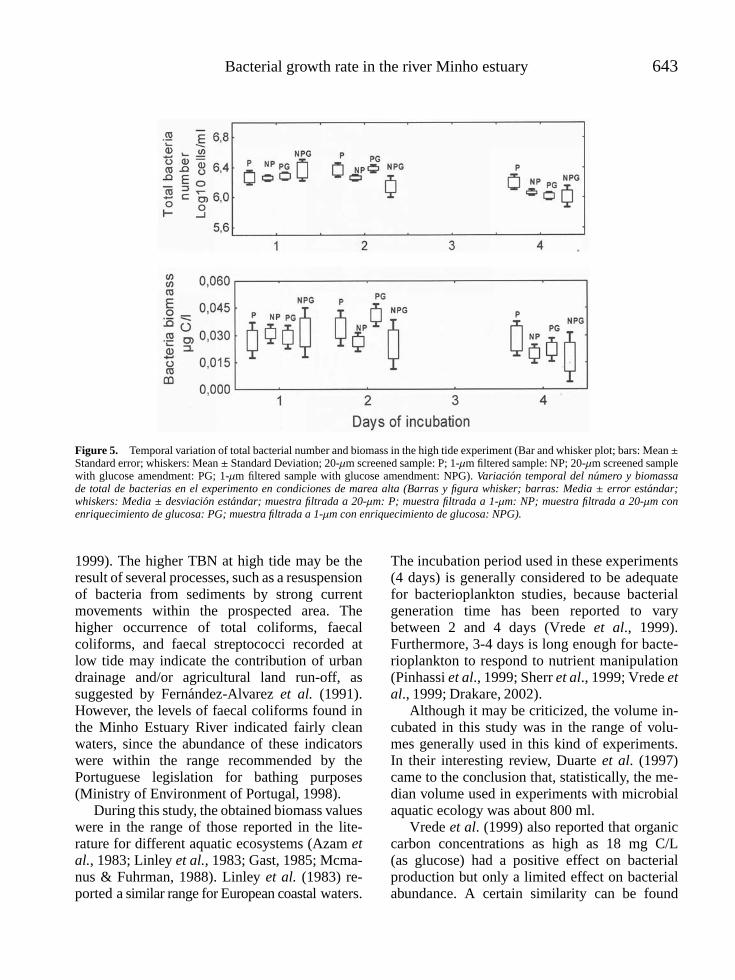
Bacterial growth rate in the river Minho estuary 643
Figure 5. Temporal variation of total bacterial number and biomass in the high tide experiment (Bar and whisker plot; bars: Mean ±Standard error; whiskers: Mean ± Standard Deviation; 20-µm screened sample: P; 1-µm filtered sample: NP; 20-µm screened samplewith glucose amendment: PG; 1-µm filtered sample with glucose amendment: NPG). Variacion temporal del numero y biomassade total de bacterias en el experimento en condiciones de marea alta (Barras y figura whisker; barras: Media ± error estandar;whiskers: Media ± desviacion estandar; muestra filtrada a 20-µm: P; muestra filtrada a 1-µm: NP; muestra filtrada a 20-µm conenriquecimiento de glucosa: PG; muestra filtrada a 1-µm con enriquecimiento de glucosa: NPG).
1999). The higher TBN at high tide may be theresult of several processes, such as a resuspensionof bacteria from sediments by strong currentmovements within the prospected area. Thehigher occurrence of total coliforms, faecalcoliforms, and faecal streptococci recorded atlow tide may indicate the contribution of urbandrainage and/or agricultural land run-off, assuggested by Fernandez-Alvarez et al. (1991).However, the levels of faecal coliforms found inthe Minho Estuary River indicated fairly cleanwaters, since the abundance of these indicatorswere within the range recommended by thePortuguese legislation for bathing purposes(Ministry of Environment of Portugal, 1998).
During this study, the obtained biomass valueswere in the range of those reported in the lite-rature for different aquatic ecosystems (Azam etal., 1983; Linley et al., 1983; Gast, 1985; Mcma-nus & Fuhrman, 1988). Linley et al. (1983) re-ported a similar range for European coastal waters.
The incubation period used in these experiments(4 days) is generally considered to be adequatefor bacterioplankton studies, because bacterialgeneration time has been reported to varybetween 2 and 4 days (Vrede et al., 1999).Furthermore, 3-4 days is long enough for bacte-rioplankton to respond to nutrient manipulation(Pinhassi et al., 1999; Sherr et al., 1999; Vrede etal., 1999; Drakare, 2002).
Although it may be criticized, the volume in-cubated in this study was in the range of volu-mes generally used in this kind of experiments.In their interesting review, Duarte et al. (1997)came to the conclusion that, statistically, the me-dian volume used in experiments with microbialaquatic ecology was about 800 ml.
Vrede et al. (1999) also reported that organiccarbon concentrations as high as 18 mg C/L(as glucose) had a positive effect on bacterialproduction but only a limited effect on bacterialabundance. A certain similarity can be found

644 Anne et al.
with our study, although we used a lower glucoseconcentration (1 mg C/L). These observations arein agreement with Caron et al. (2000), who foundno stimulatory or marginal effects of glucoseamendment on bacterial production and growthin oligotrophic waters. Using the same rangeof glucose concentration to create a gradient oforganic amendment (0.3 to 30 mg C/L), Drakare(2002) compared competition ability betweenheterotrophic bacteria and picophytoplankton.
As described by Fidalgo (1998), the MinhoEstuary River is an oligo-mesotrophic costalzone with low nutrient content (P and N). Thiscan indicate that the weak variation of bacterialabundance may be related to inorganic nutrientlimitation. Thus, to enhance bacterial growth, theaddition of these nutrients in the experimentaldesign should have been considered, and it willbe taken into account in future works.
Some of the smallest heterotrophic nanofla-gellates may have been able to pass through1 µm pore size filters, and Mcmanus & Fuhrman(1988) report evidence that up to 50 % of the gra-zing activity (heterotrophic nanoflagellates) canpass 0.6 µm pore-size filters. If this was the case,four days of incubation was enough time for na-noflagellates to increase in abundance and reducebacterial biomass in the 1 µm treatments of thehigh tide water experiment. This effect would bein accordance with Lebaron et al. (1999), whoreported a rapid control of bacterioplankton bio-mass by protozoan grazing in batch mesocosms.
The delay of two days to increase bio-mass in screened samples in the high tide ex-periment could be the result of a “shift-up”in bacterial metabolic activity and a simulta-neous lag-phase for protozoan predators be-fore reaching sufficient density to allow themto control bacterial biomass in the subse-quent days as observed by Sherr et al. (1999).
Comparing the experiments at both tidal con-ditions, it was clear that bacterial specific growthrates were significantly higher at low tide than athigh tide. These differences can be compared toresults reported by Schultz & Ducklow (2000),who reported significant differences in patternsof bacterioplankton community metabolic capa-bilities along the salinity gradient of an estuary
in Virginia. Cunha et al. (2000, 2001) found evi-dence of enhanced bacterial densities, glucose in-corporation and biomass production in brackishwater comparing with marine water in a Por-tuguese estuarine system; their findings can becompared to the tidal effects found in the pre-sent study and can help to explain why growthrates were much lower at high tide compared tothe low tide experiment (Fig. 4).
These results seem to lead to a possibleabsence or decrease of grazing impact ofpredators in filtered samples. On the other hand,nutrient increase in filtrates via cell disruptioncan also favour bacterial growth (Ferguson et al.,1984; Sherr et al., 1999). Both effects could havealso jointly resulted in the observed increase ofthe bacterial growth rate in our filtered samples.
Furthermore, the calculated bacterial specificgrowth rates in the Minho Estuary Riverwere within the range reported by Mcmanus& Fuhrman (1988) for marine waters; ourresults were, however, in the lower end ofthe range reported by Pulido-Villena & Reche(2003) who stated values of bacterial specificgrowth rates that ranged from 0.26 to 3.34day−1 for a comprehensive range of aquaticecosystems. Nonetheless, it must be emphasizedthat these authors referred to experimentalsituations without mineral nutrient limitation.
In conclusion, the physical and chemicalconditions observed during the two tidal eventsof the Minho Estuary River can be consideredas typical for oligo-mesotrophic costal zones.Although not expected, the bacterial abundancewas higher during the high tide, probablydue to hydrodynamics and resuspension ofbacteria from the sediment. The abundanceof faecal indicators was higher at low tideconditions, probably as a result of continental andagricultural land run-off influence.
Glucose amendment was not found to havea clear stimulating effect on bacterial growth inthe described experiments with water samplesfrom the oligo-mesotrophic waters of the MinhoEstuary River. This result seems to indicate thatthe supplemented concentration may have beeninsufficient, and/or bacterioplankton growth mayhave been limited by inorganic nutrients.

Bacterial growth rate in the river Minho estuary 645
This study needs to be continued in orderto better understand some fundamental aspectsconcerning interactions between bacteria andheterotrophic nanoflagellates in the studiedestuary, by tackling in more detail the size andbiomass distribution as well as growth rates ofthese two groups of micro-organisms.
ACKNOWLEDGEMENTS
This study was partially supported by CII-MAR (Centre for Marine and Environmental Re-search), and by a grant to Ibrahima Anne fromthe FCT-Foundation for Science and Technology(Grant: PRAXIS XXI/BD/13946/97).
REFERENCES
APHA. 1992. Standard Methods for the Examina-tion of Water and Wastewater, 18th ed. Washing-ton DC, USA: American Public Health Asso-ciation/American Water Works Association/WaterEnvironment Federation.
AZAM, F., T. FENCHEL, J. G. FIELD, J. S. GRAY,L. A. MEYER-REIL &. F. THINGSTAD. 1983.The ecological role of water-column microbes inthe sea. Mar. Ecol. Prog. Ser., 10: 257-263.
AZEVEDO, M. F. 1995. Comparison of some bacte-rial organisms abundance in the water and in the bi-valve mollusc Mytilus galloprovincialis Lamarck,from the Minho estuary River. M.Sc. thesis, Uni-versity of Porto. 63 pp (in Portuguese).
CALBET, A., M. L. LANDRY & S. NUNNERY.2001. Bacteria-flagellate interactions in the micro-bial food web of the oligotrophic subtropical NorthPacific. Aquat. Microb. Ecol., 23: 283-292.
CARON, D. A., E. L. LIM, R. W. SANDERS, M. R.DENNET & U-G. BERNINGER. 2000. Responseof bacterioplankton and phytoplankton to organicand inorganic nutrient additions in contrastingoceanic ecosystems. Aquat. Microb. Ecol., 22:175-184.
CHRISTOFFERSEN, K., T. AHL & O. NYBROE.1995. Grazing of nonindigenous bacteria by nano-sized protozoa in a natural coastal system. Microb.Ecol., 30: 67-78.
CUNHA, M. A., M. A. ALMEIDA & F. ALCAN-TARA. 2000. Patterns of ectoenzymatic and
heterotrophic activities along a salinity gradient ina shallow tidal estuary. Mar. Ecol. Prog. Ser., 204:1-12.
CUNHA, M. A., M. A. ALMEIDA & F. ALCAN-TARA. 2001. Short-term responses of the naturalplanktonic bacterial community to the changingwater properties in an estuarine environment:ectoenzymatic activity, glucose incorporation, andbiomass production. Microb. Ecol., 42: 69-79.
DRAKARE, S. 2002. Competition between pico-planktonic cyanobacteria and heterotrophic bacte-ria along crossed gradients of glucose and phosp-hate. Microb. Ecol., 44: 327-335.
DUARTE, C. M., J. M. GASOL & D. VAQUE.1997. Role of experimental approaches in marinemicrobial ecology. Aquat. Microb. Ecol., 13: 101-111.
FATTAL, B., E. PELEG-OLEVSKY, Y. YOSHPE-PURER & H. I. SHUVAL. 1986. The associationbetween morbidity among bathers and microbialquality of seawater. Wat. Sci. Techn., 18: 59-69.
FERGUSON, R. L., E. N. BUCKLEY & A. V. PA-LUMBO. 1984. Response of marine bacterio-plankton to differential filtration and confinement.Appl. Environ. Microbiol., 47: 49-55.
FERNANDEZ-ALVAREZ, R. M., S. CARBALLO-CUERVO, M. C. DE LA ROSA-JORGE & J.RODRIGUEZ-DE LECEA. 1991. The influence ofagricultural run-off on bacterial populations in ariver. J. Appl. Bacteriol., 70: 437-442.
FIDALGO, M. L. 1998. Contribution to the ecolo-gical characterisation of the river Minho estuary(Northern Portugal). Verh. Internat. Verein. Lim-nol., 26: 1448-1451.
FOWLER, J., L. COHEN & P. JARVIS. 1998.Practical statistics for field biology, 2nd ed. NewYork: John Wiley & Sons. 259 pp.
GAST, V. 1985. Bacteria as a food source formicrozooplankton in the Schlei Fjord and BalticSea with special reference to ciliates. Mar. Ecol.Prog. Ser., 22: 107-120.
GOLTERMAN, H. L., R. S. CLYMO & M. A. M.OHNSTAD. 1978. Methods for physical andchemical analysis of fresh waters, IBP Handbookno 8, 2nd ed. Oxford, London, Edinburgh,Melbourne: Blackwell Scientific Publications. 213pp.
HANSEN, B. & K. CHRISTOFFERSEN. 1995. Spe-cific growth rates of heterotrophic plankton orga-nisms in a eutrophic lake during a spring bloom. J.Plankton Res., 17: 413-430.

646 Anne et al.
LEBARON, P., P. SERVAIS, M. TROUSSELLIER,C. COURTIES, J. VIVES-REGO, G. MUYZER,L. BERNARD, T. GUINDULAIN, H. SCHAFER& E. STACKEBRANDT. 1999. Changes in bacte-rial community structure in seawater mesocosmsdiffering in their nutrient status. Aquat. Microb.Ecol., 19: 255-267.
LINLEY, E. A. S., R. C. NEWELL & M. I. LUCAS.1983. Quantitative relationships between phyto-plankton, bacteria and heterotrophic microflage-llates in shelf waters. Mar. Ecol. Prog. Ser., 12:77-89.
LORENZEN, C. J. 1967. Determination of chlo-rophyll and phaeopigments: spectrophotometricequations. Limnol. Oceanogr., 12: 343-346.
MARSALEK, J., B. J. DUTKA & I. K. TSANIS.1994. Urban impacts on microbiological pollutionof the St Clair river in Sarnia, Ontario. Wat. Sci.Tech., 30 (1): 177-184.
MCMANUS, G. B. 1993. Growth rates of naturalpopulations of heterotrophic nanoplankton. In:Handbook of methods in aquatic microbialecology. Kemp P., Sherr, B., Sherr E. & Cole J.(eds.): 557-562. Lewis Publishers, Boca Raton.
MCMANUS, G. B. & J. A. FUHRMAN. 1988. Con-trol of marine bacterioplankton populations: mea-surement and significance of grazing. Hydrobiolo-gia, 159: 51-62.
MINISTRY OF ENVIRONMENT OF PORTUGAL.1998. Law no 236/98 of 1st of August. Diarioda Republica, I Serie-A, 176: 3676-3718. (inPortuguese).
NORLAND, S. 1993. The relationship between bio-mass and volume of bacteria. In: Handbook of met-hods in microbial ecology. Kemp P., Sherr, B.,Sherr E. & Cole J. (eds): 303-307. Lewis Publis-hers, Boca Raton.
NYBROE, O., K. CHRISTOFFERSEN & B. RIE-MANN. 1992. Survival of Bacillus licheniformisin seawater model ecosystems. Appl. Environ. Mi-crobiol., 58: 252-259.
PINHASSI, J., F. AZAM, J. HEMPHALA, R. A.LONG, J. MARTINEZ, U. L. ZWEIFEL & A.HAGSTROM. 1999. Coupling between bacterio-plankton species composition, population dyna-mics, and organic matter degradation. Aquat. Mi-crob. Ecol., 17: 13-26.
PINHEIRO, A. & M. L. FIDALGO. 2000. Contribu-tion for the study of bacterioplankton of the riverMinho estuary (Portugal). Verh. Internat. Verein.Limnol., 27: 1890-1893.
PORTER, K. G. & Y. S. FEIG. 1980. The useof DAPI for identifying and counting aquaticmicroflora. Limnol. Oceanogr., 25: 943-948.
PULIDO-VILLENA, E. & I. RECHE. 2003. Explo-ring bacterioplankton growth and protein synthesisto determine conversion factors across a gradientof dissolved organic matter. Microb. Ecol., 46: 33-42.
SCHULTZ, G. E. & H. DUCKLOW. 2000. Changesin bacterioplankton metabolic capabilities along asalinity gradient in the York river Estuary, Virginia,USA. Aquat. Microb. Ecol., 22: 163-174.
SHERR, B. F., E. B. SHERR & C. PEDROS-ALIO.1989. Simultaneous measurement of bacterio-plankton production and protozoan bacterivory inestuarine water. Mar. Ecol. Prog. Ser., 54: 209-219.
SHERR, E. B., B. F. SHERR & C. T. SIGMON.1999. Activity of marine bacteria under incubatedand in situ conditions. Aquat. Microb. Ecol., 20:213- 223.
SUZUKI, M. 1999. Effect of protistan bacterivory oncoastal bacterioplankton diversity. Aquat. Microb.Ecol., 20: 261-272.
USEPA. 1986. Ambient water quality criteria forbacteria. Washington, DC 20460. EPA 440/5-84-002.
VREDE, K., T. VREDE, A. ISAKSSON & A.KARLSSON. 1999. Effects of nutrients (phospho-rus, nitrogen and carbon) and zooplankton on bac-terioplankton and phytoplankton-a seasonal study.Limnol. Oceanogr., 44: 1616-1624.
Limnetica, 25 (3-4): xx-xx (2006)Limnetica, 25 (3): 657-664 (2006)c© Asociacion Espanola de Limnologıa, Madrid. Spain. ISSN: 0213-8409
Influence of habitat structure on the fish prey consumption bylargemouth bass, Micropterus salmoides, in experimental tanks
Francisco Nunes Godinho1,2,∗ and Maria Teresa Ferreira2
1 Centro de Estudos Florestais - Departamento de Engenharia Florestal, Instituto Superior de Agronomia, Tapadada Ajuda, 1349-017 Lisboa, Portugal.2 Conselho Nacional da Agua, Rua de S. Domingos a Lapa, n.o 26, 1200-835 Lisboa, Portugal.3 Hola∗ Corresponding author: [email protected]
ABSTRACT
Influence of habitat structure on the fish prey consumption by largemouth bass, Micropterus salmoides, in experimentaltanks
The largemouth bass, Micropterus salmoides, was introduced into the Iberian Peninsula in the 50’s and has developedimportant populations in systems naturally lacking native piscivores. As a consequence, the displacement of native cyprinidshas been associated with its predatory behaviour, particularly in reservoirs. In order to study the capture rate of largemouth bassin relation to an Iberian native cyprinid, Squalius alburnoides, and also to pumpkinseed, Lepomis gibbosus –another exoticspecies introduced to Iberia that is able to coexist sucessfully with bass in Iberian systems-tanks were used to simulate theabsence of structure, and the presence of vegetation struture and bottom structure. The number of fish captured by largemouthbass were influenced by both structure and prey effects, as well as by their interaction. The bottom and vegetation structurereduced the number of pumpkinseed captured when compared with the absence of structure, whereas only the vegetationreduced the number of Squalius alburnoides captured. Neither the pumpkinseed nor the cyprind were eaten more frequentlyby largemouth bass in the absence of structure or in the vegetation structure, but the cyprinid was eaten more frequently in thebottom structure.
Key words: Largemouth bass, pumpkinseed, iberian cyprinids, habitat.
RESUMEN
Influencia de la estructura del habitat en el consumo de peces presa por la perca americana, Micropterus salmoides, enexperimentos en tanques
El black bass, Micropterus salmoides, fue introducido en la Penınsula Iberica en los anos 50 y ha desarrollado importantespoblaciones en sistemas naturalmente carentes de ictiofagos nativos. Como consecuencia, el aparente desplazamiento delos ciprınidos nativos ha sido asociado con su comportamiento predador, particularmente en embalses. Con el objetivode estudiar la captura del black bass sobre un ciprınido iberico nativo, el calandino, Squalius alburnoides y sobre el pezsol, Lepomis gibbosus –otra especie exotica introducida en Iberia que es capaz de coexistir con exito con el black bassen los sistemas ibericos– se utilizaron tanques simulando tres situaciones: ausencia de estructuras, estructuras vegetales yestructuras de ladrillos. Se comprobo que el numero de peces capturados por el black bass estaba influenciado por el efecto delas estructuras y de las presas, ası como por su interaccion. Las estructuras vegetales y de ladrillo provocaban una reduccionen el numero de pez sol capturadas en comparacion con la ausencia de tales estructuras, mientras que instalando soloestructuras vegetales el numero de calandinos, Squalius alburnoides, capturados disminuıa. El black bass no capturo ningunade las dos especies en mayor numero en ausencia de estructuras o en estructuras vegetales, pero capturo el calandino masfrecuentemente en presencia de estructuras de ladrillo.
Palabras clave: Black bass, pez sol, ciprınidos nativos, habitat.
Hola

658 Godinho & Ferreira
INTRODUCTION
In southern Iberia, the primary piscivorous(sensu Keast 1985) largemouth bass, Micropterussalmoides, was introduced in the fifties intonative fish communities naturally lacking thistype of predatory fish (Almaca, 1983 and 1986;Collares-Pereira, 1985; Elvira 1995a). Sincethen it has rapidly spread and has long beenblamed as the main cause for the apparentdisplacement of small sized endemic cyprinidsin central and southern basins (Almaca, 1983;Elvira 1995a; Pires et al., 1999). For example,in a southern basin, assemblages of endemicsmall sized cyprinids were found to be spatiallysegregated from largemouth bass as well as frompumpkinseed sunfish, Lepomis gibbosus, anotherNorth American centrarchid later introduced intoIberia (Almodovar & Elvira, 1994; Godinho etal., 1997a). This other exotic species rapidlybecame associated with largemouth bass both inreservoirs and rivers (Braband & Saltveit, 1989;Almodovar & Elvira, 1994; Godinho & Ferreira,1997; Godinho et al., 1997a and 1998) and itis presently the bass’ chief prey in southernaquatic systems (Godinho & Ferreira, 1994 and1997, Nicola et al., 1996; Godinho et al., 1997b).Nevertheless, some field data has suggested thatbass may favour the endemic cyprinids overpumpkinseed as prey (Godinho et al., 1997b).
The present rare coexistence of largemouthbass and small Iberian cyprinids, given the bass’apparent selection for these, and the positiveassociation of bass and pumpkinseed, couldsuggest a distinct capture success of bass of bothprey types. Furthermore, in the correlative studiesof Godinho & Ferreira (1994) and Godinho etal. (1997b), fish prey were eaten less frequentlywhen submerged macrophytes were abundant.Experimental studies have also revealed thatincreasing levels of structural complexity, in theform of submerged vegetation, influences bassforaging rate for other fish prey species such asthe pumpkinseed congeneric, and the bluegill,Lepomis macrochirus (Gotceitas & Colgan,1989; Savino & Stein 1982, 1989a and 1989b).
In this study we tested the effects of differentprey types, pumpkinseed vs endemic Iberian
Table 1. Two-way ANOVA for the effects of prey andstructure type on the foraging rate (number of fish eaten during21 hours) of largemouth bass in experimental tanks. ANOVA dedos factores para los efectos de la presa y el tipo de estructurasobre la tasa de capturas (numero de peces consumidos en 21horas) por los black bass en los tanques experimentales.
df Mean square F p
Prey (pumpkinseed vscyprinids) 1 10.80 16.20 <0.001Structure type 2 13.73 20.60 <0.001Prey × structure type 1 2.80 4.20 <0.05Residual 24 0.67
cyprinid, and aquatic structure types, on theforaging rate of largemouth bass in experimentalfeeding trials. So far, the controled experimentsconducted to analyse the effects of habitatstructure on largemouth bass capture rates for fishprey have only considered different densities ofsubmerged macrophytes (Savino & Stein, 1982;Schramm & Zale, 1985; Gotceitas & Colgan,1989; Savino & Stein, 1989a and 1989b).Since distinct types of structure influence theforaging rate of other fish predators differently(Christensen & Persson, 1993), we investigatednot only the effects of vegetation structure butalso those of bottom structure.
MATERIAL AND METHODS
Experiments were conducted in three outdoorshaded plastic tanks (white walls, 1 m2, 0.5 mdeep with rounded edges) located in Tapadada Ajuda, Lisboa Portugal, during the Autumn.Three kinds of aquatic structure were tested:no structure, simulated vegetation (henceforthreferred to as vegetation structure) and simulatedbottom crevices (henceforth referred to as bottomstructure). The vegetation structure consistedof 0.5 m strings (4 mm in diameter) ofgreen polypropylene attached to the bottom andcovering 1/4 of the tank area (i.e. 0.25 m2)with a density of 1000 stems m−2, a densitypreviously found to provide effective refuge frombass predation for the bluegill (Savino & Stein,1982). The bottom structure consisted of onebrick 0.30 × 0.15 × 0.40 m presenting 5 × 3squared holes with 50 mm sides. The brick was

Fish consumption by bass in experimental tanks 659
Figure 1. Number (mean of five replicates ± 1 SE) of fish captured during 21 hours by largemouth bass in tanks simulating differentstructure types. P-pumpkinseed, and C-Cyprinid, whereas ns-no structure, vs-vegetation structure and bs-bottom structure. Lettersfor prey and structure types are combined to represent a particular treatment. Bars within a prey type followed by the same letterare not significantly different (post-ANOVA Tukey HSD, p > 0.05). Numero de peces (media de cinco replicas ± 1 SE) capturadosdurante 21 horas por los black bass en los tanques simulando diferentes tipos de estructuras. P-caladinos, y C-ciprinıdos, mientrasque ns-sin estructura, vs-estructura con vegetacion y bs-estuctura en el fondo. Las letras para las presas y el tipo de estructuras estancombinadas para presentar un determinado tipo de tratamiento. Las barras dentro de un tipo de seguidas de la misma letra no sonsignificativamente diferentes (a partir de un ANOVA Tukey HSD, p > 0.05).
placed at the bottom of the tank against one ofthe tank sides and it allowed the access of prey tothe holes but not of bass. The bottoms of all tankswere covered by a layer of gravel.
Fishes used in the experiments were collectedin nearby rivers and ponds by electrofishing andseine nets. Besides largemouth bass (275-280mm in total length TL) and pumpkinseed (40-75 mm in TL), one Iberian cyprinid was used,the Iberian roach, Squalius alburnoides (40-80mm in TL). This cyprinid is widespread in Iberiaand often dominates native fish assemblages(Doadrio et al., 1991; Peris et al., 1994; Collares-Pereira et al., 1995; Elvira 1995b).
All the fishes were housed in the experimen-tal area where they were acclimatized to exis-ting conditions for two months before use. Du-ring that period, bass were fed pumpkinseed androach, whereas the cyprinid and pumpkinseed atefrozen adult Artemia salina and pieces of earth-worm. Each individual bass was allowed to feedin the three structure types at least six times be-fore the experiment began. Tanks were oxyge-
nated (to about 7 mg/l) with a pump and 20 %of the water in each tank was renovated bet-ween trials. Turbidity was always below 4 JTU.
Capture rates were examined in single preytype trials (with either five pumpkinseed or fiveroach) and in mixed prey type trials (with fivepumpkinseed plus five roach).
Each trial began when naive prey werereleased (after 15 min aclimatization in a plasticbag) with a bass starved for 24 hours (previouslyacclimatized for two hours) in a tank presentingone of the structure types tested. Trials beganat 2p.m. (local time) after prey fish had beenreleased in the tank and ended at 11a.m. thenext day, i.e. after 21 hours. At the end of theexperiment each bass was feed to satiation andthe surviving prey counted. Further, the locationof the tank occupied by surviving prey was noted.
The different structure types, as well as preytypes (in the single prey type trials), wererandomnly assigned to each of the three tanksavailable before each trial. The six bass usedwere divided in two groups of three and each

660 Godinho & Ferreira
group was used during each day. Within agroup, each bass was randomly assigned tothe treatments being tested in a particular day.In the single prey experiments all treatmentswere replicated 5 times. Mixed prey trialswere replicated five or six times. The effectsof structure and prey type (i.e. pumpkinseedor Iberian cyprinid) on the foraging rate oflargemouth bass (in the single prey experiments)were analysed with a two-way ANOVA and post-ANOVA Tukey HSD tests (Wilkinson, 1990). Nodifferences were noted in the overall foragingrate for both prey and structure type between thetwo bass groups ( p > 0.05 in-all comparisons)and the data was therefore lumped for analysis.
RESULTS
Daily fluctuations in the water temperatureduring the course of the experiment were wide(from a minimum of 15 ◦C to a maximum of24 ◦C) and were mainly a consequence of thedaily normal oscillations of the air temperatureoccuring in Portugal at this time of the year.Nevertheless, minimum as well as maximumwater temperatures (measured with maximum-minimum thermometers) were not significantlydifferent in the various treatments ( p > 0.05).Moreover, bass appeared to forage willinglywhile facing the experimental conditions.
Overall, the two factors tested, as well astheir interaction, influenced the number of fishcaptured by bass (Table 1), with the cyprinidbeing captured in higher numbers than thepumpkinseed (Fig. 1). The presence of bothbottom and vegetation structures reduced thenumber of pumpkinseed captured by bass whencompared with the numbers captured in theabsence of any structure. In contrast, onlythe vegetation structure significantly reducedthe number of cyprinid captured by bass. Allsurvivors (both prey types) collected in thevegetation and bottom structures were withinthe vegetation patch or inside the brick holes.The few survivors collected in the absence ofstructure were allways at the tank bottom edge.
In the mixed prey trials no preference (i.e.,
Table 2. Number of mixed prey type trials where largemouthbass took higher, equal, or lower numbers of pumpkinseed thancyprinid. Numero de experimentos con mezcla de presas en losque los black bass atraparon un numero mayor, menor o igualde caladinos que ciprınidos.
No Vegetation Bottomstructure structure structure
Pumpkinseed > cyprinids 1 2 0Pumpkinseed < cyprinids 4 3 5Pumpkinseed = cyprinids 1 1 0
more frequent consumption) was detected foreither prey (pumpkinseed or cyprinid) in theabsence of structure (χ2 = 6.44, df = 5, ANOVAcomparing numbers of prey eaten in 21 hours F= 4.16, p = 0.07) and in the vegetation structure(χ2 = 5.86, df = 5, F = 0.776, p = 0.39),but cyprinids were eaten more frequently in thebottom structure (χ2 = −16.5, df = 4; F =14.6, p = 0.005). Nevertheless, the cyprinid wastaken in higher numbers than the pumpkinseedin more trials (Table 2).
DISCUSSION
In general, the results obtained in this studysupport the largemouth bass patterns of fish preyuse observed in southern Iberia, with endemiccyprinids being captured at higher rates thanthe pumpkinseed (Godinho et al., 1997b). InNorth American rivers and lakes, species of smallcyprinids are also captured faster than both thebluegill and pumpkinseed (Savino & Stein, 1989;Hambright et al., 1991; Mittelbach et al., 1995).In fact, small sized North American species ofCyprinidae such as Pimephales promelas andNotemigonus crysoleucas are usually rare in thepresence of largemouth bass whereas Lepomisspp. can sustain large populations (e.g. Johanneset al., 1987, Hambright et al., 1991; Mittelbachet al. 1995). These community patterns parallelthe present spatial organization observed in manysouthern Iberian freshwater systems (Almodovar& Elvira, 1994; Godinho & Ferreira, 1994;Godinho et al., 1997a; Pires et al., 1999).
Factors such as the low handling timecyprinids (narrow-bodied with soft fin rays)

Fish consumption by bass in experimental tanks 661
present when compared with the sunfish (deep-bodied with spiny fin rays) probably wereinvolved in the bass higher capture rates forthe Iberian roach (Hoyle & Keast, 1987;Hambright, 1991). According to Webb (1986),the deeper body of the bluegill (and thepumpkinseed), compared with the one of acyprinid (P. promelas), tended to shift thepredator attack target from the middle-bodytowards the head or tail, thereby increasingthe number of prey escapes and unsuccessfulbass attacks. Behavioural differences between thetwo prey types could also have resulted in thedifferent capture determined. Non quantitativeobservations made during the course of ourtrials suggested that roach and pumpkinseedbehave differently in the presence of largemouthbass. For instance, after their introduction into atank the roach usually wandered and eventuallyapproached bass at a much closer distancethan the pumpkinseed. In addition, roach wasusually found much closer to the surface whereaspumpkinseed were closer to the bottom.
As already demonstrated in other studies,the capture of fish prey by bass decreases inthe presence of dense stands of aquatic plants(Savino & Stein, 1982, 1989a and, 1989b) andin this study we have shown that it decreasesin the presence of bottom structure as well.According to Savino & Stein (1982), this ismostly caused by the reduction in bass visualcontact, and thus encounter rates, with prey.In our study, both the bottom and vegetationstructure did indeed reduce pumpkinseed capturerate, and this species quickly sought refuge inthe vegetation patch or in the holes. However,only the vegetation structure decreased thecapture of Iberian roach. Roach is related toabundant macrophyte stands in Iberian rivers(Collares-Pereira et al., 1995, Godinho et al.,1997) and this association probably reducedtheir capture rate in the simulated vegetationtreatment. In contrast to pumpkinseed, roachdid not penetrate the brick holes in the bottomstructure (personal observation) and possiblyremained as vulnerable in that treatment as it wasin the absence of structure. Consequently, bassclearly demonstrated a higher roach consumption
when offered together with pumpkinseed in thebottom structure.
Reductions in the predator foraging rate inthe presence of structure have been theoretica-lly shown to have a stabilizing effect on predator-prey relationships (Murdoch & Oaten, 1975), andthus to be important forces in the organization offish assemblages (Christensen & Persson, 1993).Structure such as vegetation and rocks are perva-sive elements of aquatic freshwater environments(Anderson, 1984), but their relative importanceis system specific. In Iberian lowland rivers, towhich roach is adapted (Collares-Pereira et al.,1995, Godinho et al. and 1997a), macrophyticcover is usually high (Ferreira, 1994; Ferreira &Moreira, 1996). River damming, especially forirrigation purposes, results in extreme fluctua-tions of the water levels in reservoirs (Garcia deJalon, 1992). Permanent disturbance, apart fromother regulation side-effects (Petts, 1988), doesnot favour the development and permanence ofmacrophyte stands on reservoir margins, therebychanging the type of aquatic cover from one do-minated by vegetation structure to another do-minated by bottom structure. Despite the invol-vement of other factors, we suggest that the ha-bitat alterations resulting from impoudment, thatchanges the relative vulnerability of different fishprey, contribute to the absence (or low abun-dance) of roach in reservoirs and the developmentof abundant pumpkinseed populations in the pre-sence of bass (Godinho et al., 1998).
ACKNOWLEDGMENTS
We would like to acknowledge Antonio Albu-querque for his useful collaboration during therunning of the experiments.
REFERENCES
ALMACA, C. 1983. Contemporary changes in Por-tuguese freshwater fish fauna and conservationof autochtonous Cyprinidae.-Roczniki Nauk Rol-niczych, Seria 9-15.

662 Godinho & Ferreira
ALMACA, C. 1986. Fish and their environmentin large European river ecosystems Tejo andGuadiana. Sciences de 1’ Eau, 7: 3-19.
ALMODOVAR, A. & B. ELVIRA. 1994. Furtherdata on the fish fauna catalogue of the natural parkof Ruidera lakes (Guadiana river basin, centralSpain). Verh. Int. Verein. Limnol., 25: 2173-2177.
ANDERSON, O. 1984. Optimal foraging by large-mouth bass in structured environments. Ecology,65: 851-861.
BRABAND, A. & S. J. SALTVEIT. 1989. Ecologicalaspects of the fish fauna in three Portuguesereservoirs. Arch. Hydrobiol., 114: 575-589.
CHRISTENSEN, C. & L. PERSSON. 1993. Species-specific antipredatory behaviours: effects on preychoice in different habitats. Behav. Ecol. Socio-biol., 32: 1-9.
COLLARES-PEREIRA, M. J. 1985. Ciprinıdeos doAlentejo. In: Primeiro Congresso sobre o Alentejo.Associacao dos Municipeos de Beja, Alentejo,Portugal: 537-545.
COLLARES-PEREIRA, M. J., M. F. MAGALHAES,A. M. GERALDES, & M. M. COELHO. 1995.Riparian ecotones and spatial variation of fishassemblages in Portuguese lowland streams.Hydrobiologia, 303: 93-101.
DOADRIO, I., B. ELVIRA, & Y. BERNAT. 1991.Peces continentales Espanoles –ColeccionTecnica, Instituto Nacional para la Conservationde la Naturaleza. Madrid. 221 pp.
ELVIRA, B. 1995a. Native and exotic freshwaterfishes in Spanish river basins. Freshwat. Biol., 33:103-108.
ELVIRA, B. 1995b. Conservation status of endemicfreshwater fish in Spain. Biol. Conserv., 72: 129-136.
FERREIRA, M. T. 1994. Aquatic and marginal vege-tation of river Divor and its relation with land use.Verh. Int. Verein. Limnol., 25: 2309-2316.
FERREIRA, M. T. & I. MOREIRA. 1996. Theinvasive component of a river flora under theinfluence of Mediterranean agricultural systems.In: Plant Invasions, General Aspects and SpecialProblems. Pysek, P., K. Prach, M. Rejmanek, & M.Wade (eds.): 117-127. SPB Academic Publishing,Amsterdan, The Netherlands.
GARCIA DE JALON, D. G., M. G. TANAGO & C.CASADO. 1992. Ecology of regulated streams inSpain: An overview. Limnetica, 8: 161-166.
GODINHO, F. N. & M. T. FERREIRA. 1994. Dietcomposition of largemouth black bass, Micropte-rus salmoides Lacepede in southern Portuguese re-servoirs: its relation to habitat characteristics. Fish.Manage. Ecol., 1: 129-137.
GODINHO, F. N. & M. T. FERREIRA. 1997. Theapplication of size-structure indices to Micropterussalmoides and Lepomis gibbosus as a managementtool for southern Iberian reservoirs. PublicacionesEspeciales Instituto Espanol Oceanografia, 21:275-281.
GODINHO, F. N., M. T. FERREIRA & R. V. COR-TES. 1997a. Composition and spatial organizationof fish assemblages in the lower Guadiana basin,southern Iberia. Ecol. Fresh. Fish 6: 134-143.
GODINHO, F. N., M. T. FERREIRA & R. V. COR-TES. 1997b. The environmental basis of diet va-riation in pumpkinseed sunfish, Lepomis gibbo-sus, and largemouth bass, Micropterus salmoides,along an Iberian river basin. Env. Biol. Fish., 50:105-115.
GODINHO, F. N., FERREIRA, M. T. & PORTU-GAL-CASTRO M. I. 1998. Fish assemblage com-position in relation to environmental gradients inPortuguese reservoirs. Aquatic Living Resources,11: 325-334.
GOTCEITAS, V. & P. COLGAN. 1989. Predator fo-raging success and habitat complexity: quantita-tive test of the threshold hypothesis. Oecologia,80: 158-166.
HAMBRIGHT, K. D. 1991. Experimental analysisof prey selection by largemouth bass: role ofpredator mouth width and prey body depth. Trans.Amer. Fish. Soc., 120: 500-508.
HAMBRIGHT, K. D., R. W. DRENNER, S. R. MC-COMAS & N. G. HAIRSTON JR. 1991. Gape-limited piscivores, planktivore size refuges, andthe trophic cascade hypothesis, Arch. Hydrobiol.,121: 389-404.
HOYLE, J. A. & A. KEAST. 1987. The effect ofprey morphology and size on handling time ina piscivore, the largemouth bass (Micropterussalmoides). Can. J. Zool., 65: 1972-1977.
JOHANNES, M. FIT. S., D. J. MCQUEEN, T. J.STEWART & J. R. POST. 1989. Golden shiner(Notemigonus crysoleucas) population abundance:correlations with food and predators. Can. J. Fish.Aquat. Sci., 46: 810-817.
KEAST, A. 1985. The piscivore feeding guild offishes in small freshwater ecosystems. Env. Biol.Fish., 12: 119-129.

Fish consumption by bass in experimental tanks 663
MITTELBACH, G. G., M. TURNER, D. J. HALL &J. E. RETTIG. 1995. Perturbation and resilience: along term whole-lake study of predator extinctionand reintroduction. Ecology, 76: 2347-2360.
MURDOCH, W. W. & A. OATEN 1975. Predationand population stability. Adv. Ecol. Res., 9: 1-131.
NICOLA, G. G., A. ALMODOVAR & B. ELVIRA.1996. The diet of introduced largemouth bass,Micropterus salmoides, in the natural park of theRuidera lakes, central Spain. Pol. Arch. Hydrobiol.,43: 179-184.
PERIS, S. J., A. MARTIN & J. C. VELASCO. 1994.Age, growth and reproduction of the cyprinid Tro-pidophoxinellus alburnoides (Stephanidis, 1974)in river Agueda, westcentral Spain. Arch. Hydro-biol., 131: 341-352.
PETTS, G. E. 1988. Impounded Rivers. -Wiley, Chi-chester. 326 pp.
PIRES, A. M., I. G. COWX & M. M. COELHO.1999. Seasonal changes in fish community struc-ture of intermittent streams in the middle reachesof the Guadiana basin, Portugal. J. Fish Biol., 54:235-249.
SAVINO, J. F. & R. A. STEIN. 1982. Predator-preyinteractions between largemouth bass and bluegillas influenced by simulated, submerged vegetation.Trans. Amer. Fish. Soc., 111: 255-266.
SAVINO, J. F. & R. A. STEIN. 1989a. Behaviouralinteractions between fish predators and their prey:effects of plant density. Anim. Behav., 37: 311-321.
SAVINO, J. F. & R. A. STEIN. 1989b. Behavior offish predators and their prey: habitat. Env. Biol.Fish. 24: 287-293.
SCHRAMM, H. L. & A. V. ZALE. 1985. Effects ofcover and prey size on preferences of juvenilelargemouth bass for blue tilapias and bluegills intanks. Trans. Amer. Fish. Soc., 114: 725-731.
WEBB, P. W. 1986. Effect of body form and res-ponse treshhold on the vulnerability of four speciesof teleost prey attacked by largemouth bass (Mi-cropterus salmoides). Can. J. Fish. Aquat. Sci., 43:763-771.
WILKINSON, L. 1990. SYSTAT: the system. forstatistics. SYSTAT, Evanston, Illinois, USA.choice between open water and dense vegetation.Env. Biol. Fish., 24: 287-293.


Limnetica, 25 (3-4): xx-xx (2006)Limnetica, 25 (3): 665-682 (2006)c© Asociacion Espanola de Limnologıa, Madrid. Spain. ISSN: 0213-8409
Crustacean and aquatic insect assemblages in the Mediterraneancoastal ecosystems of Emporda wetlands (NE Iberian peninsula)
Monica Martinoy1, Dani Boix2, Jordi Sala2, Stephanie Gascon2, Jaume Gifre1, Alba Argerich2,Ricard de la Barrera1, Sandra Brucet2, Anna Badosa2, Rocıo Lopez-Flores2, MontserratMendez2, Josep Maria Utge2, Xavier D. Quintana2,∗
1 Servei de Control de Mosquits de la Badia de Roses i Baix Ter.2 Institut d’Ecologia Aquatica, Universitat de Girona. Facultat de Ciencies, Campus Montilivi, E-17071,Girona, Spain.2 Institut∗ Corresponding author: [email protected]
ABSTRACT
Crustacean and aquatic insect assemblages in the Mediterranean coastal ecosystems of Emporda wetlands (NE Iberianpeninsula)
Coastal wetlands are characterized by high biodiversity, which is one of the main criteria considered when establishingprotection policies or when proposing adequate management actions. In this study, the crustacean and aquatic insectcomposition of the Emporda wetlands is described. These two faunal groups contribute highly to the total biodiversity inthese wetlands but are seldom considered when managing natural areas. A selection (84 sampling points) of all water bodytypes present in the Emporda wetlands were sampled monthly (surber and dip net with a 250 µm mesh). Sampling was carriedout during 3 surveys (1991-92, 1996-97 and 1999-2000). A rich fauna of 125 crustacean and 295 aquatic insect taxa wasidentified. We characterized each water body type using the most abundant species and the relative species richness of thetaxonomic groups. A classification of the water body types, according to similarity between inventories, groups the brackishand hyperhaline systems in one cluster and the various freshwater systems in another one. Among freshwater systems, loticwaters and freshwater wetlands have a high similarity, whereas rice fields and freshwater springs have a low similarity.
Key words: Mediterranean coastal wetlands, water body types, composition, species richness, crustaceans, aquatic insects.
RESUMEN
Comunidades de crustaceos e insectos acuaticos en los ecosistemas costeros mediterraneos de los Aiguamolls del Emporda(NE de la penınsula Iberica)
Los humedales costeros se caracterizan por una alta biodiversidad, que es uno de los principales criterios considerados alestablecer polıticas de proteccion o al proponer acciones de gestion adecuada. En este estudio se describe la composicion decrustaceos e insectos acuaticos de los aiguamolls del Emporda. Estos dos grupos faunısticos contribuyen de forma importanteal total de la biodiversidad en los humedales, pero raramente se tienen en consideracion al gestionar las areas naturales. Semuestreo mensualmente una seleccion (84 puntos de muestreo) de todas las tipologıas de masas de agua presentes en losaiguamolls de l’Emporda mediante redes surber y salabres de poro de malla de 250 µm. El muestreo se llevo a cabo durantetres campanas (1991-92, 1996-97 y 1999-2000). Se identifico una riqueza faunıstica de 125 taxones de crustaceos y 295taxones de insectos acuaticos. Cada tipologıa de masa de agua se caracterizo utilizando las especies mas abundantes yla riqueza especıfica de los grupos faunısticos. La clasificacion de las tipologıas de masas de agua, segun la similaridadentre inventarios faunısticos, agrupo los sistemas salobres y hiperhalinos en un grupo. Entre los sistemas de agua dulce, lossistemas loticos y los humedales de agua dulce presentaron una alta similaridad, mientras que los arrozales y las surgenciasde agua dulce mostraron una baja similaridad.
Palabras clave: Humedales costeros mediterraneos, tipologıa de masas de agua, composicion, riqueza especıfica, crustaceos,insectos acuaticos.

666 Martinoy et al.
INTRODUCTION
Wetlands, marshes, ponds and other permanentor temporary shallow waters have increasinglyattracted conservation biologists during the lastyears. Several studies underline their ecologicalimportance indicating that they not only containspecies or environments that are becoming ra-rer, but also have a high specific richness (Giu-dicelli & Thiery, 1998; Gopal & Junk, 2000;Boix et al., 2001). Despite the fact that theirimportance has been recognized in the Euro-pean Directive that considers them as priori-tary habitats (92/43/CEE), these ecosystems arestill under the threat of degradation and loss(Tagliapietra et al., 1998; Brown, 1998; Mis-tri et al., 2000; Gibbs, 2000). Biodiversity isone of the main criteria used when elaboratingwetland protection policies (Ramsar ConventionBureau, 1992). Invertebrates are the most im-portant proportion of faunal richness, but theknowledge of wetland aquatic invertebrate spe-cies composition is still relatively poor, and mostmanagement efforts today are being focused onthe conservation of a small number of species,mainly water birds (Britton, 1982; Mocci, 1983).
The aim of this paper is to present currentknowledge on the composition of crustaceansand aquatic insects of different water bodytypes in a group of Mediterranean coastalwetlands (Emporda wetlands), located in the NEIberian Peninsula. Emporda wetlands present awide range of environmental types, due to theexistence of high gradients of salinity, waterpermanence, and nutrients.
STUDY AREA
The Emporda wetlands are located in the north-eastern part of the Iberian Peninsula. They aresituated in a deltaic plain originated by quater-nary depositions from the Muga, Fluvia, Ter, andDaro rivers. The Montgrı massif divides the del-taic plain in two halves, which are connected in-land (Fig. 1). The wetlands in the northern partof the deltaic plain are larger and protected bythe Emporda Wetlands Natural Park (4731 ha).
Conversely, the protection status of the wetlandsof the southern part of the plain is weaker, andrestricted to the larger lagoons. The hydrology ofthe littoral wetlands is influenced by the sea, andis characterised by sudden and irregular flood-ing (caused by sea storms, rainfall and inputsfrom rivers or channels), followed by dry pe-riods, when most of the basins become isolatedand gradually dry out (Bach, 1990; Quintana,2002). The hydrology of the inland wetlandsis influenced by rainfall and river inputs (su-perficial or groundwater), and marine influenceis scarce or inexistent (Trobajo et al., 2002).
METHODS
Quantitative sampling was carried out monthlyduring three different surveys (1991-92, 1996-97,1999-2000), each of them including different wa-ter bodies. For detailed information about sam-pling surveys see Gifre et al. (1996), Sala et al.(1998) and Quintana et al. (2000). Besides thesesurveys, qualitative samplings have been carriedout during the last fifteen years, in order to de-tect rare species. All sampled water bodies (84sampling points) are shown in figure 1 Additionalqualitative data were obtained from the literature.
Sampling in lentic ecosystems was conductedusing a dip-net 20 cm in diameter and 250 µmmesh size. In each water body 20 dip-netsweeps (sweeps were done by pushes in arapid sequence) per visit were carried out. Inlotic ecosystems, sampling was done using thedip-net and a surber net with a 30 × 30 cmopening and 1 mm mesh size.
All water bodies were grouped into thedifferent environmental types found in the studyarea, following Trobajo et al. (2002). Thisclassification is based on the physical, chemicaland biological characteristics of 22 water bodiesfrom the study area. Because this classificationdid not encompass all types of water bodiesin the area, we included 4 more types (loticwaters, ephemeral brackish wetlands, ephemeralfreshwater wetlands, and rice fields). Some of thephysical, chemical, and biological characteristicsof each water body type are shown in Table 1.

Crustacean and aquatic insect assemblages of Emporda wetlands 667
Table 1. Physical, chemical, and biological characteristics of each water body type of the Emporda wetlands. Mean values in boldand coefficients of variation in italics. Legend: HHW: hyperhaline wetlands; BW: brackish wetlands; HTW: hypertrophic freshwaterwetlands; MFW: meso-eutrophic freshwater wetlands; FS: freshwater springs; LW: lotic waters; EBW: ephemeral brackish wetlands;EFW: ephemeral freshwater wetlands; RF: rice fields; —: no data available. Caracterısticas fısicas, quımicas y biologicas de lasdiferentes tipologıas de masas de agua de los aiguamolls del Emporda. Valores medios en negrita y coeficientes de variacionen cursiva. Leyenda: HHW: humedales hiperhalinos; BW: humedales salobres; HTW: humedales hipertroficos de agua dulce;MFW: humedales meso-eutroficos de agua dulce; FS: surgencias; LW: sistemas loticos; EBW: humedales salobres efımeros; EFW:humedales de agua dulce efımeros; RF: arrozales; —: datos no disponibles.
Waterbody types
HHW BW HTW MFW FS LW EBW EFW RF
Approximated hydroperiod length 12 7-12 12 7-12 12 12 <2 <2 7
(months·year−1)
Conductivity 49.6 18.9 1.3 3.9 1.1 0.8 6.9 1.4 1.2
(mS·cm−1) 48 66 136 179 99 76 96 39 39
Chlorophyll-a 21.5 20.9 12.1 14.3 18.1 6.5 — — —
(µg·L−1) 186 183 107 150 143 103
Ammonium 9.1 4.3 34.1 8.6 2.6 29.8 — — —
(µM) 196 260 109 245 351 214
Nitrite 0.7 0.5 6.9 2.0 5.5 10.9 — — —
(µM) 569 234 156 289 148 193
Nitrate 2.1 11.1 109.9 53.7 705.9 205.6 — — —
(µM) 253 312 58 151 25 100
Phosphate 4.3 3.7 5.8 2.9 0.93 8.5 — — —
(µM) 298 253 173 174 368 159
Total N 219.3 164.8 212.7 125.0 851.9 — — — —
(µM) 160 94 49 75 27
Total P 10.5 9.2 11.0 6.1 2.0 — — — —
(µM) 248 213 83 121 197
RESULTS AND DISCUSSION
Faunal composition of the Emporda wetlands
A remarkable rich fauna including 420 taxawas found in the studied area, 125 of whichwere crustaceans and 295 aquatic insects (Table2). Within the crustaceans, Copepoda andBranchiopoda were the best represented classes(41 and 42 taxa respectively), followed byOstracoda (24 taxa) and Malacostraca (18 taxa).Within the aquatic insects, Coleoptera (129taxa), Diptera (94 taxa), Odonata (36 taxa), andHeteroptera (25 taxa) were the richest orders,together representing 97 % of the insect taxa
found in the area. Following these orders wereEphemeroptera (7 taxa), Trichoptera (2 taxa),Neuroptera (1 taxon), and Plecoptera (1 taxon).A reverse pattern is observed when abundanceis taken into account, crustaceans (mainlyBranchiopoda, Copepoda and Ostracoda) beingfar more abundant than aquatic insects. Withinthe insects, Diptera and some species ofEphemeroptera and Odonata were the mostabundant taxa in the studied area.
Several crustacean species collected in theEmporda wetlands are rare in the Iberian Penin-sula. This is the case of the exotic cladoceranWlassicsia pannonica, which has only been cap-tured in the rice fields of Badajoz (M. Alonso,

668 Martinoy et al.
Figure 1. Map of the study with the location of the 84 water bodies studied. Shaded symbols correspond to qualitative samples,whereas open symbols correspond to quantitative samples. Mapa del area de estudio con la localizacion de las 84 masas de aguaestudiadas. Los sımbolos grises corresponden a muestras cualitativas, mientras que los sımbolos blancos corresponden a muestrascuantitativas.
pers. com.). Similarly, several ostracod speciessuch as Fabaeformiscandona fabaeformis, Pota-mocypris variegata, Limnocythere inopinata, No-todromas persica, and Bradleystrandesia reticu-lata, are barely known in the Iberian Peninsula
(Baltanas et al., 1996), and are first citations forthe region of Catalunya. The calanoid Euryte-mora velox has its southern limit of distributionin the Emporda wetlands. Among the insects,some coleopteran species have a special inte-

Crustacean and aquatic insect assemblages of Emporda wetlands 669
rest, such as Cyphon laevipennis, which is ci-ted for the first time in the Iberian Peninsula,although it is abundant in common reeds in theEmporda wetlands. Ochthebius gr. maculatus andTanysphyrus lemmnae are first cited for Cata-lunya. The former species is frequently obser-ved in salt marshes, while the latter one is espe-cially abundant in rice fields. The coleopteransGeorissus sp., Megasternum sp., Helophorus ru-fipes, Cymbiodita marginella, and Cercyon ter-minatus are rarely found in the Iberian Penin-sula. Other insects found in our study are alsorare, such as the heteropterans Gerris asper (firstcitation in Catalunya), Sigara selecta, and Me-sovelia vittigera. The coleopteran Cercyon sp.1seems to be a species not included in the checklistof the Iberian water beetles (Ribera et al., 1998)(C. Hernando, pers. com.).
The number of first faunal citations obtai-ned in this initial attempt to describe the inver-tebrate biodiversity of Emporda wetlands, evi-dences the lack of information regarding in-vertebrate distribution in the area. This ma-kes the development of conservation strate-gies to avoid biodiversity loss a difficult task.Although some proposals exist, they consideronly a specific group such as coleopterans. Inone of these proposals (Ribera, 2000), Stenelmisconsobrina appears as a species in need of pro-tection, and several other coleopterans (Chasmo-genus livornicus, Graphoderus cinereus, Hydati-cus seminiger, Hygrotus parallelogrammus, Ily-bius quadriguttatus, Helophorus illustris, Cym-biodyta marginella and Hydrochara caraboi-des) are shown as having few known popula-tions in the Iberian Peninsula.
A revision of the material during this studyhas also detected some misidentifications. Thisis the case of Heterocypris barbara, cited inGifre et al. (2002), which corresponds to juvenileH. incongruens. Similarly, Mesochra rapiens,cited in Appendix II in Martinoy et al. (2004),corresponds to M. heldti, whereas Upogebiatipica and Palaemon elegans, which were citedby Vila et al. (1989), correspond to U. pusillaand P. adpersus, respectively. Finally, Haliplusruficollis, found by Lagar (1968), was attributedto Haliplus heydeni by Rico et al. (1990).
Invertebrate composition of the differentwater body types
Hyperhaline wetlands (HHW) were dominatedin terms of richness by microcrustacean taxa.The best represented species (higher abundances)were the calanoids Eurytemora velox and Calani-peda aquaedulcis, while cladocerans were veryscarce. Coleoptera and Diptera had also high ri-chness in this water body type. Coleoptera asNebrioporus ceresyi, Ochthebius dentifer, Helop-horus fulgidicollis, Berosus hispanicus, and theCulicidae Ochlerotatus detritus were characteris-tic of this water body type (Fig. 2 and Table 2).
Brackish wetlands (BW) differ from hyper-haline ones in the higher richness of Malacos-traca and Heteroptera found in them (Fig. 2). Op-posite to HHW, brackish wetlands had a higherrichness of insects due to the appearance ofnew taxa (such as ephemeropterans, trichopte-rans, and heteropterans). Moreover, some crus-taceans found in the previous wetland type werealso found in BW, but their relative importancewas different (Table 2). Thus, in this water bodytype, high abundances of some copepods suchas Acanthocyclops spp., Cyclops sp., Thermocy-clops dybowskii, and Cletocamptus confluens,as well as some ostracods such as Loxocon-cha elliptica and Cypridopsis vidua were cha-racteristic. High abundances of cladocerans suchas Ceriodaphnia dubia and Daphnia pulicariawere found coinciding with lower salinity values.
Basins with freshwater inputs of treated was-tewater or agricultural origin (i.e., with high nu-trient concentrations) were classified as hyper-trophic freshwater wetlands (HTW). This typeof wetland is characterised by an irregular wa-ter flux conditioned by human management. Insuch conditions, cladocerans had the highest ri-chness (Fig. 2). As for abundance, some cyclo-poids (Eucyclops serrulatus and Macrocyclopsalbidus) and cladocerans (Bosmina longirostris),even benthic ones (Tretocephala ambigua), weredominant. Insects were dominated by Chirono-midae larvae (Table 2).Freshwater wetlands (FW), with a less artificialflooding pattern, encompassed a heterogeneousgroup of basins (drainage channels, either inland

670 Martinoy et al.
Figure 2. Taxonomic composition of each water body type.The relative species richness of each taxonomic group is shown.The figures in brackets indicate the total richness of each waterbody type. Composicion taxonomica de cada masa de agua.Se representa la riqueza especıfica relativa de cada grupotaxonomico. Los numeros entre parentesis indican la riquezatotal de cada tipo de masa de agua.
or coastal freshwater basins, and alluvial basins)with some similarities: (1) low salinity values,although subjected to sporadic marine waterinputs, and (2) relatively high concentrations ofnutrients, but always lower than those reportedin the hypertrophic freshwater wetlands. Inthese environments, the cyclopoid Acanthocy-clops spp. was dominant during situationswith high water turnover rate, while thecalanoid Calanipeda aquaedulcis was dominantin confinement situations with low water inputs.Coleoptera was the group with the highestspecific richness, Ochthebius dilatatus being themost abundant species (Fig. 2 and Table 2).
Freshwater springs (FS) were characterisedby groundwater circulation with low phosphateconcentrations, and small temperature and sali-nity oscillations. They also presented high den-sities of submerged macrophytes. As in the pre-vious water body type (FW), Coleoptera was therichest taxonomic group (Fig. 2), Hydroglyphusgeminus being the most abundant (Table 2). Thelower taxonomic resolution used for non-bitingmidges (Chironomidae) in this water body typecould explain, almost partially, the lower valueof dipteran richness obtained. Regarding abun-dance, the microcrustacean assemblage was cha-racterised by the cyclopoid Eucyclops serrula-tus and the cladoceran Chydorus sphaericus (Ta-ble 2). Additionally, species generally associatedwith macrophytes were also found to be abun-dant (Cypridopsis vidua and Pleuroxus aduncus;Alonso, 1996; Meisch, 2000). The high abun-dance of some insects that were scarcer in otherlentic systems, such as Cloeon inscriptum, Nau-coris maculatus and Anopheles atroparvus, wasalso characteristic of this water body type.
Lotic waters (LW), included all types ofrunning waters present in the study area,from channels, fluvial sites, and river mouths(which are characterized by an estuarine beha-viour with slow water circulation) to tempo-rary streams. Coleopterans had the highest ri-chness in this water body type (Fig. 2), butthe most abundant organisms were the cladoce-ran Chydorus sphaericus, followed by the co-pepod Eucyclops serrulatus and the non-bitingmidge Polypedilum sp. (Table 2).

Crustacean and aquatic insect assemblages of Emporda wetlands 671
No quantitative data were available for epheme-ral wetlands, either brackish (EBW) or fresh-water (EFW), and qualitative data were not ob-tained for all taxonomic groups, so their faunalcomposition cannot be correctly assessed. Howe-ver, the presence of large branchiopods (Bran-chipus schaefferi and Triops cancriformis), bothin fresh and brackish waters, was characteristicof these habitats. The other large branchiopodpresent in the studied area, Chirocephalus dia-phanus, was only found in ephemeral freshwaterwetlands. Note that mosquitoes had a high num-ber of species in these water body types (Table2). Ochlerotatus caspius and Ochlerotatus detri-tus were characteristic of brackish waters, whilethe remaining species were found in fresh waters.
In rice fields (RF) the most abundanttaxa were cladocerans, Moina macrocopus,Chydorus sphaericus and the exotic Wlassicsiapannonica being particularly relevant (Table 2).Among the insects, two ephemeropteran species(Caenis luctuosa and Cloeon inscriptum) and
the biting midges (Ceratopogonidae) had highabundances. Species richness was dominated bycladocerans and dipterans (together representingapproximately 50 % of total richness; Fig. 2).
Comparison of the assemblages observed ineach water body type (Fig. 3) identifies salinityas the most important factor regulating speciescomposition, as has been previously stated in se-veral studies (Britton & Johnson, 1987; Timms,1993; Cognetti & Maltagliati, 2000). Thus, thetwo water body types with higher salinities, bra-ckish wetlands and hyperhaline wetlands, appearclearly separated from the rest of the water bodytypes (Fig. 3). Among freshwater water body ty-pes, three of them (freshwater wetlands, lotic wa-ters, and hypertrophic freshwater wetlands) showa high similarity, while freshwater springs andrice fields show a different composition. Accor-ding to the position of the freshwater body ty-pes in the cluster, hypertrophy and water fluxseem to be less important for assemblage com-position than artificial water regimes and oligo-
MFW
LW
HTW
FS
RF
HHW
BW
Figure 3. Dendrogram showing the classification of water body types by the similarity of their faunal inventories. Presence/Absencedata, average linkage as a cluster method, and Dice measurement as similarity distance were used. Dendrograma mostrandola clasificacion de las tipologıas de masas de agua segun la similaridad de los inventarios faunısticos. Se utilizaron datos depresencia/ausencia, la vinculacion inter-grupos como metodo de conglomeracion, y la medida de Dice como distancia de similaridad.
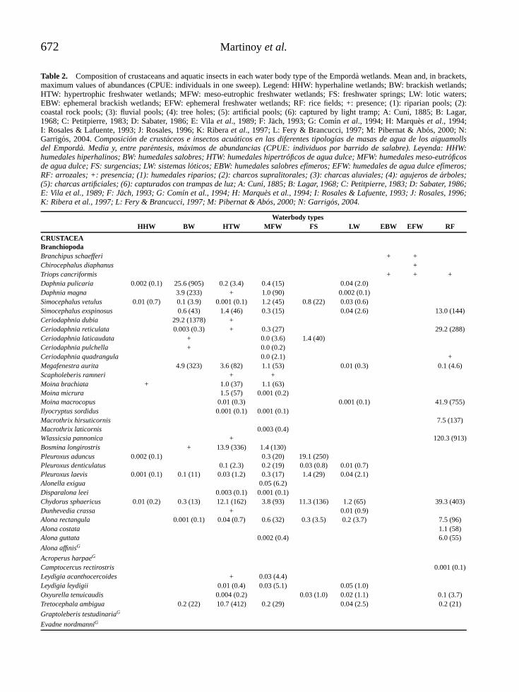
672 Martinoy et al.
Table 2. Composition of crustaceans and aquatic insects in each water body type of the Emporda wetlands. Mean and, in brackets,maximum values of abundances (CPUE: individuals in one sweep). Legend: HHW: hyperhaline wetlands; BW: brackish wetlands;HTW: hypertrophic freshwater wetlands; MFW: meso-eutrophic freshwater wetlands; FS: freshwater springs; LW: lotic waters;EBW: ephemeral brackish wetlands; EFW: ephemeral freshwater wetlands; RF: rice fields; +: presence; (1): riparian pools; (2):coastal rock pools; (3): fluvial pools; (4): tree holes; (5): artificial pools; (6): captured by light tramp; A: Cunı, 1885; B: Lagar,1968; C: Petitpierre, 1983; D: Sabater, 1986; E: Vila et al., 1989; F: Jach, 1993; G: Comın et al., 1994; H: Marques et al., 1994;I: Rosales & Lafuente, 1993; J: Rosales, 1996; K: Ribera et al., 1997; L: Fery & Brancucci, 1997; M: Pibernat & Abos, 2000; N:Garrigos, 2004. Composicion de crustaceos e insectos acuaticos en las diferentes tipologıas de masas de agua de los aiguamollsdel Emporda. Media y, entre parentesis, maximos de abundancias (CPUE: individuos por barrido de salabre). Leyenda: HHW:humedales hiperhalinos; BW: humedales salobres; HTW: humedales hipertroficos de agua dulce; MFW: humedales meso-eutroficosde agua dulce; FS: surgencias; LW: sistemas loticos; EBW: humedales salobres efımeros; EFW: humedales de agua dulce efımeros;RF: arrozales; +: presencia; (1): humedales riparios; (2): charcos supralitorales; (3): charcas aluviales; (4): agujeros de arboles;(5): charcas artificiales; (6): capturados con trampas de luz; A: Cunı, 1885; B: Lagar, 1968; C: Petitpierre, 1983; D: Sabater, 1986;E: Vila et al., 1989; F: Jach, 1993; G: Comın et al., 1994; H: Marques et al., 1994; I: Rosales & Lafuente, 1993; J: Rosales, 1996;K: Ribera et al., 1997; L: Fery & Brancucci, 1997; M: Pibernat & Abos, 2000; N: Garrigos, 2004.
Waterbody typesHHW BW HTW MFW FS LW EBW EFW RF
CRUSTACEABranchiopodaBranchipus schaefferi + +Chirocephalus diaphanus +Triops cancriformis + + +Daphnia pulicaria 0.002 (0.1) 25.6 (905) 0.2 (3.4) 0.4 (15) 0.04 (2.0)Daphnia magna 3.9 (233) + 1.0 (90) 0.002 (0.1)Simocephalus vetulus 0.01 (0.7) 0.1 (3.9) 0.001 (0.1) 1.2 (45) 0.8 (22) 0.03 (0.6)Simocephalus exspinosus 0.6 (43) 1.4 (46) 0.3 (15) 0.04 (2.6) 13.0 (144)Ceriodaphnia dubia 29.2 (1378) +Ceriodaphnia reticulata 0.003 (0.3) + 0.3 (27) 29.2 (288)Ceriodaphnia laticaudata + 0.0 (3.6) 1.4 (40)Ceriodaphnia pulchella + 0.0 (0.2)Ceriodaphnia quadrangula 0.0 (2.1) +Megafenestra aurita 4.9 (323) 3.6 (82) 1.1 (53) 0.01 (0.3) 0.1 (4.6)Scapholeberis ramneri + +Moina brachiata + 1.0 (37) 1.1 (63)Moina micrura 1.5 (57) 0.001 (0.2)Moina macrocopus 0.01 (0.3) 0.001 (0.1) 41.9 (755)Ilyocryptus sordidus 0.001 (0.1) 0.001 (0.1)Macrothrix hirsuticornis 7.5 (137)Macrothrix laticornis 0.003 (0.4)Wlassicsia pannonica + 120.3 (913)Bosmina longirostris + 13.9 (336) 1.4 (130)Pleuroxus aduncus 0.002 (0.1) 0.3 (20) 19.1 (250)Pleuroxus denticulatus 0.1 (2.3) 0.2 (19) 0.03 (0.8) 0.01 (0.7)Pleuroxus laevis 0.001 (0.1) 0.1 (11) 0.03 (1.2) 0.3 (17) 1.4 (29) 0.04 (2.1)Alonella exigua 0.05 (6.2)Disparalona leei 0.003 (0.1) 0.001 (0.1)Chydorus sphaericus 0.01 (0.2) 0.3 (13) 12.1 (162) 3.8 (93) 11.3 (136) 1.2 (65) 39.3 (403)Dunhevedia crassa + 0.01 (0.9)Alona rectangula 0.001 (0.1) 0.04 (0.7) 0.6 (32) 0.3 (3.5) 0.2 (3.7) 7.5 (96)Alona costata 1.1 (58)Alona guttata 0.002 (0.4) 6.0 (55)
Alona affinisG
Acroperus harpaeG
Camptocercus rectirostris 0.001 (0.1)Leydigia acanthocercoides + 0.03 (4.4)Leydigia leydigii 0.01 (0.4) 0.03 (5.1) 0.05 (1.0)Oxyurella tenuicaudis 0.004 (0.2) 0.03 (1.0) 0.02 (1.1) 0.1 (3.7)Tretocephala ambigua 0.2 (22) 10.7 (412) 0.2 (29) 0.04 (2.5) 0.2 (21)
Graptoleberis testudinariaG
Evadne nordmanniG

Crustacean and aquatic insect assemblages of Emporda wetlands 673
Waterbody typesHHW BW HTW MFW FS LW EBW EFW RF
CopepodaErgasilus sp. +Calanipeda aquaedulcis 19.0 (387) 100.9 (2326) 0.0 (0.7) 23.6 (1325) 0.8 (18) + 0.1 (2.1)Acartia bifilosa +Acartia clausi +Acartia margalefiG
Eurytemora velox 47.6 (1356) 39.6 (1098) 0.001 (0.1) 0.1 (3.7) +Mixodiaptomus kupelwieseri 2.1 (104) 0.004 (0.3)Halicyclops magniceps 0.001 (0.001) +Halicyclops rotundipes 0.5 (15) 0.1 (2.0) 0.01 (0.9) 0.0 (0.2)Macrocyclops albidus 6.6 (221) 0.2 (8.9) 2.4 (21) 0.3 (12) 0.2 (7.4)Eucyclops serrulatus 0.0 (0.2) 0.6 (29) 13.8 (479) 0.6 (14) 22.2 (339) 1.9 (44)Tropocyclops prasinus 0.0 (0.5) 0.006 (0.4) 0.6 (8.2) 0.0 (0.8) 0.3 (7.0)Paracyclops affinis 0.0 (0.1) 0.6 (16)Paracyclops fimbriatus 0.01 (0.2) 0.01 (1.1) 0.0 (1.4) 0.1 (3.2)Ectocyclops phaleratus 0.01 (0.1) 0.01 (0.6) 0.004 (0.1)Cyclops sp. 0.1 (1.9) 7.0 (100) 1.5 (84) 0.1 (2.4)Megacyclops viridis 0.0 (2.3) 0.02 (2.0) 7.1 (97)Megacyclops gigas 0.001 (0.1)Acanthocyclops spp. 0.1 (1.3) 41.4 (1677) 10.7 (103) 15.6 (451) 1.5 (32) 0.7 (6.7) 10.9 (84)Diacyclops bicuspidatus 0.01 (0.4) 0.6 (51) 0.2 (15) 0.001 (0.1) +D. bicuspidatus odessanus 2.3 (51) 41.4 (821) 0.003 (0.1) 0.6 (29) 0.002 (0.1) +Diacyclops bisetosus 0.5 (20) 0.5 (28) +Microcyclops varicans 0.01 (0.4) 0.02 (3.5) 0.02 (1.6)Microcyclops rubellus 0.1 (8.3) 0.9 (24)Thermocyclops dybowskii 1.0 (51) 0.2 (7.7) 0.2 (24) 0.7 (24)Canuella perplexa 1.8 (30) 0.4 (23) 0.004 (0.4)Phyllognathopus viguieri 0.002 (0.3)Harpacticus littoralis 0.1 (1.4) 0.001 (0.1) 0.001 (0.1)Tigriopus fulvus 0.1 (2.9) 0.001 (0.2)Tisbe longicornis 0.4 (14) 0.001 (0.1) +Nitokra lacustris 0.1 (2.4) 0.02 (1.5) 0.02 (2.6)Nitokra spinipes 0.1 (2.4) 0.001 (0.1) 0.02 (3.1) +Bryocamptus minutus +
Bryocamptus pygmaeusD
Canthocamptus staphylinus 0.003 (0.1) 0.03 (2.4) 1.8 (28) 0.02 (0.4)Mesochra lilljeborgi + + +Mesochra heldti 1.5 (21) + 0.5 (6.0) 0.1 (5.4) 0.05 (1.1)Cletocamptus confluens 0.002 (0.1) 0.5 (15)Onychocamptus mohammed 0.002 (0.3)Paronychocamptus nanus +
Paraleptastacus spinicaudaD
Parastenocaris sp.D
OstracodaCyprideis torosa 1.4 (37) 0.8 (23) 0.02 (2.0) 0.01 (0.4)Limnocythere inopinata 0.005 (0.3)Loxoconcha elliptica 0.003 (0.2) 0.5 (34)Ilyocypris gibba 0.2 (20) +Fabaeformiscandona fabaeformis 0.003 (0.1)Cypria ophtalmica 0.002 (0.2) 0.001 (0.2) 0.8 (22)Notodromas monacha 0.001 (0.2)Notodromas persica 0.1 (6.8)Heterocypris incongruens 0.1 (2.7) 0.2 (8.8) 0.003 (0.2) + +Heterocypris salina 0.01 (0.7) + + + +Eucypris virens 0.004 (0.3) 0.4 (11) 1.1 (75) 0.5 (17)Bradleystrandesia reticulata 0.02 (1.3) 0.01 (1.3)Isocypris beauchampi 0.002 (0.1)Herpetocypris brevicaudata 0.8 (11)

674 Martinoy et al.
Waterbody typesHHW BW HTW MFW FS LW EBW EFW RF
Herpetocypris chevreuxi + +Cypris bispinosa +Cypretta seurati +
Cypridopsis parva G
Cypridopsis vidua 0.2 (10) 0.5 (32) 0.04 (1.2) 1.4 (74) 16.5 (207) 0.2 (3.7)Plesiocypridopsis newtoni 2.6 (101) 0.03 (4.3) 0.1 (3.0)Potamocypris arcuata + +Potamocypris variegata 0.004 (0.1) 0.04 (5.4) 0.02 (1.1)Potamocypris villosa 0.02 (0.8)Sarscypridopsis aculeata 0.1 (5.8) + 0.1 (3.7) 0.002 (0.2)
MalacostracaMesopodopsis slabberi 0.04 (1.1) 0.1 (7.4) 0.02 (1.5) 0.005 (0.2)Siriella clausi +Heterotanais oerstedii 0.001 (0.3) 0.01 (0.3)Proasellus coxalis 0.01 (0.4) 0.003 (0.1) 0.02 (1.2) 0.003 (0.1) 0.01 (0.2)Lekanesphaera hookeri 0.2 (8.2) 0.3 (11) 0.1 (5.1) 0.02 (0.4)Protracheoniscus occidentalis + + + + +Leptocheirus pilosus +Corophium orientale 0.02 (1.9) 0.03 (2.7) 0.01 (0.3)Echinogammarus longisetosus 0.1 (1.1)Gammarus aequicauda 0.1 (2.3) 0.5 (8.6) 0.1 (7.9) 0.002 (0.1) +Orchestia sp. + 0.002 (0.1)Parahyale eburnea +Talorchestia cf. deshayesii +Atyaephyra desmarestii 0.002 (0.2) 0.001 (0.1) 0.1 (4.8) 0.002 (0.1) 0.1 (4.3)
Palaemon adpersus E
Upogebia pusilla E
Carcinus aestuarii +Procambarus clarkii + + + + +
INSECTAEphemeropteraBaetis rhodani +Baetis nigrescens +Baetis gr. lutheri +Cloeon inscriptum 0.02 (0.7) 0.02 (0.3) 0.1 (6.0) 2.5 (16) 0.2 (7.9) + 9.9 (133)Caenis luctuosa 0.001 (0.1) 0.3 (18) 39.3 (528)Habrophlebia fusca +Ephoron virgo +
PlecopteraNemoura sp. +
OdonataCalopteryx xanthosoma M
Calopteryx haemorrhoidalis M
Lestes viridis 0.002 (0.2)Lestes barbarus +Lestes virens N
Sympecma fuscaN
Platycnemis latipes M
Platycnemis acutipennis M
Pyrrhosoma nymphula 0.002 0.1 0.003 0.1
Erythromma viridulum M
Coenagrion mercuriale +
Coenagrion caerulescens M
Coenagrion puella N
Cercion lindeni M
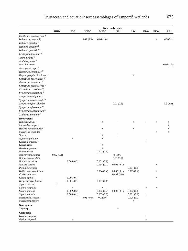
Crustacean and aquatic insect assemblages of Emporda wetlands 675
Waterbody typesHHW BW HTW MFW FS LW EBW EFW RF
Enallagma cyathigerum N
Ischnura sp. (nymph) 0.01 (0.3) 0.04 (2.0) + 4.5 (31)
Ischnura pumilio N
Ischnura elegans M
Ischnura graellsii M
Ceriagrion tenellum M
Aeshna mixta N
Aeshna cyanea M
Anax imperator 0.04 (1.5)
Anax parthenope M
Hemianax ephippiger N
Onychogomphus forcipatus +
Orthetrum cancellatum M
Orthetrum brunneum M
Orthetrum coerulescens M
Crocothemis erythrea M
Sympetrum striolatum N
Sympetrum vulgatum M
Sympetrum meridionale M
Sympetrum fonscolombii 0.01 (0.2) 0.5 (1.3)
Sympetrum flaveolum M
Sympetrum sanguineum M
Trithemis annulata N
HeteropteraHebrus pusillus + + + + + +Mesovelia vittigera +Hydrometra stagnorum + + +Microvelia pygmaea + +Velia sp. + +Aquarius paludum + +Gerris thoracicus +Gerris asper +Gerris argentatus +Nepa cinerea 0.001 (0.1)Naucoris maculatus 0.002 (0.1) 0.1 (0.7)Notonecta maculata 0.01 (0.2)Notonecta viridis 0.003 (0.2) 0.001 (0.1)Anisops sardea 0.014 (1.7) 0.006 (0.1) +Plea minutissima 0.001 (0.1)Heliocorisa vermiculata 0.004 (0.4) 0.003 (0.1) 0.003 (0.2) +Corixa punctata 0.032 (1.0)Corixa affinis 0.001 (0.1) +Hesperocorixa linnaei 0.001 (0.1) 0.001 (0.1)Sigara selecta +Sigara stagnalis + + + +Sigara dorsalis 0.002 (0.2) 0.002 (0.2) 0.002 (0.1) 0.002 (0.1)Sigara lateralis 0.003 (0.1) 0.005 (0.6) 0.001 (0.1) +Micronecta scholtzi 0.02 (0.6) 0.2 (19) 0.028 (1.0)Micronecta poweri +
NeuropteraSisyra sp. +
ColeopteraGyrinus caspius +Gyrinus dejeani + +

676 Martinoy et al.
Waterbody typesHHW BW HTW MFW FS LW EBW EFW RF
Gyrinus substriatus + +Gyrinus urinator + 0.001 (0.1) +Haliplus lineatocollis +
Haliplus heydeni B
Noterus clavicornis + 0.002 (0.2) + + 0.01 (0.2)Noterus laevis +Copelatus haemorrhoidalis + + + +Laccophilus hyalinus + + 0.01 (0.2) + 0.01 (0.2)Laccophilus minutus + +Laccophilus poecilus 0.001 (0.1) +
Hyphydrus aubei I
Hydrovatus cuspidatus +
Yola bicarinata I
Bidessus goudotii I
Bidessus minutissimus +Bidessus pumilus I
Hydroglyphus geminus + + + 0.04 (0.4) 0.002 (0.2) + + 0.001 (0.1)
Hygrotus confluens I
Hygrotus impressopunctatus + + + +Hygrotus inaequalis + +Hygrotus parallelogrammus +
Hydroporus normandi (1) + +Hydroporus planus 0.002 (0.1) 0.01 (0.3) + + + +Hydroporus pubescens + + + + + +Hydroporus tessellatus + +Hydroporus vagepictus + +
Graptodytes flavipes I
Graptodytes ignotus +
Graptodytes varius I
Graptodytes bilineatus +Metaporus meridionalis 0.01 (0.2) 0.002 (0.1) + + +
Deronectes hispanicus L
Deronectes opatrinus L
Stictotarsus duodecimpustulatus I
Nebrioporus canaliculatus +Nebrioporus ceresyi + + +
Agabus biguttatus I
Agabus bipustulatus + + + +Agabus conspersus +Agabus didymus + +Agabus nebulosus + + +Ilybius montanus + + +Ilybius quadriguttatus +Rhantus suturalis + + + 0.002 (0.1) + + + 0.004 (0.1)Colymbetes fuscus +Meladema coriacea +Eretes sticticus +Hydaticus leander + + + + + 0.001 (0.1)Hydaticus seminiger + +Graphoderus cinereus +Cybister lateralimarginalis +Helophorus rufipes +Helophorus alternans 0.001 (0.1) 0.002 (0.1) 0.001 (0.1) + +
Helophorus aequalis J
Helophorus maritimus + + +Helophorus brevipalpis 0.001 (0.1) 0.005 (0.2) 0.001 (0.1) + +

Crustacean and aquatic insect assemblages of Emporda wetlands 677
Waterbody typesHHW BW HTW MFW FS LW EBW EFW RF
Helophorus fulgidicollis 0.01 (0.5) 0.04 (0.6) + 0.002 (0.2) 0.002 (0.1) 0.006 (0.2) + +Helophorus illustris 0.001 (0.2) + +
Helophorus minutus J
Helophorus obscurus +Georissus sp.1 +Georissus sp.2 +Hydrochus flavipennis + +Hydrochus smaragdineus +Berosus affinis 0.001 (0.1) + +Berosus hispanicus 0.009 (0.4) 0.001 (0.1) 0.001 (0.1) +Berosus signaticollis 0.001 (0.1) + + +Chaetarthria similis +Paracymus aeneus 0.002 (0.1) 0.001 (0.1)Anacaena bipustulata + +Anacaena globulus +
Anacaena lutescens J
Laccobius femoralis +Laccobius gracilis +Laccobius ytenensis + + + +Laccobius striatulus +Helochares lividus + + 0.002 (0.1) + + + +Chasmogenus livornicus K
Enochrus bicolor 0.003 (0.1) 0.002 (0.1) + 0.004 0.1 + +Enochrus quadripunctatus + + + + 0.01 (0.2)Enochrus testaceus +Cymbiodyta marginella + +Hydrobius fuscipes +Limnoxenus niger + + + + +Hydrochara caraboides +Hydrophilus pistaceus + + + + +Coelostoma hispanicum +Coelostoma orbiculare 0.002 (0.1) +
Cercyon subsulcatus K
Cercyon terminatus + +
Cercyon laminatus (6) + +Cercyon sp.1 + +
Sphaeridium scarabaeoides A
Megasternum sp. +
Dactylosternum abdominale (6) + +Hydraena atrata + +Hydraena testacea +
Limnebius furcatus F
Limnebius nitidus +Aulacochthebius exaratus + + +Ochthebius quadricollis (2)
Ochthebius aeneus + 0.001 (0.1) +Ochthebius dilatatus 0.002 (0.1) 0.001 (0.1) 0.003 (0.4) 0.01 (0.1) 0.004 (0.2) + +Ochthebius gr. maculatus + + +
Ochthebius subinteger (2)
Ochthebius dentifer 0.03 (1.8) 0.003 (0.2) +
Ochthebius marinus J
Ochthebius punctatus 0.001 (0.1) + + +Ochthebius quadrifoveolatus +Ochthebius subpictus + + 0.001 (0.1) +Ochthebius viridis sp.2 sensu Jach, 1992 + +Cyphon laevipennis + + + + +Cyphon sulcicollis +Stenelmis canaliculata +

678 Martinoy et al.
Waterbody typesHHW BW HTW MFW FS LW EBW EFW RF
Stenelmis consobrina J
Esolus parallelepipedus +Oulimnius rivularis 0.001 (0.1) 0.001 (0.1)Dryops algiricus + +Dryops gracilis + + + + +Dryops luridus +Dryops nitidulus +Dryops sulcipennis +Botriophorus atomus + +Heterocerus fenestratus +Heterocerus flexuosus + +
Plateumaris sericea C
Tanysphyrus lemnae +
TrichopteraLimnephilus sp. 0.003 (0.1) 0.001 (0.3) 0.026 (1.5) +Hydropsyche sp. 0.001 (0.2) 0.005 (0.2)
DipteraTipulidae undet. 0.01 (0.2)Limoniidae undet. + 0.002 (0.1)Psychodidae undet. 0.1 (18) 0.01 (0.2) 0.007 (0.3) 0.012 (0.2)Dixidae undet. 0.02 (0.5) 0.01 (0.1) 0.03 (2.4) 0.2 (5.0) 0.005 (0.2) + 0.1 (1.9)Dixella autumnalis + + +Chaoborus crystallinus 0.3 (8.2)Anopheles atroparvus + 4.5 (129) + + + 1.7 (15)
Anopheles petragnani (3) +
Anopheles plumbeus (4)
Aedes vexans +Aedes vittatus H
Ochlerotatus geniculatus (4)
Ochlerotatus caspius + + + + +Ochlerotatus detritus 0.004 (0.2) 0.2 (4.7) + + +
Ochlerotatus mariae (2)
Ochlerotatus rusticus H
Culex hortensis H
Culex impudicus + + + + 0.001 (0.1)
Culex modestus H
Culex pipiens 0.03 (0.6) 0.002 (0.2) + 0.001 (0.1) + + +Culex theileri + + + + + 0.1 (0.5)Culiseta annulata + +Culiseta longiaerolata (5)
Culiseta litorea + +Culiseta subochrea + + +Coquillettidia buxtoni H
Coquillettidia richiardii H
Simuliidae undet. 0.01 (0.1) 0.001 (0.1) 0.6 (26)Simulium ornatum +Simulium velutinum +Ceratopogonidae undet. 0.002 (0.1) 0.02 (0.6) 0.01 (0.8) 0.1 (2.2) 0.005 (0.1) + 7.7 (244)Culicoides sp. +Chironomidae undet. 0.3 (3.5) 5.1 (19) +Monopelopia sp. 0.7 (5.5)Procladius sp. + 0.2 (3.4)Tanypus sp. +Rheopelopia sp. 0.04 (2.6)Telmatopelopia sp. 0.002 (0.1)Xenopelopia sp. 0.001 (0.1)Potthastia gr. gaedii 0.001 (0.1) 0.3 (14)
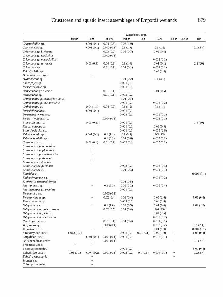
Crustacean and aquatic insect assemblages of Emporda wetlands 679
Waterbody typesHHW BW HTW MFW FS LW EBW EFW RF
Chaetocladius sp. 0.001 (0.1) 0.04 (0.6) 0.03 (1.9)Corynoneura sp. 0.001 (0.1) 0.003 (0.1) 0.1 (1.9) 0.1 (1.6) 0.1 (3.4)Cricotopus gr. bicinctus 0.03 (0.2) 0.03 (0.7) 0.03 (0.6)Cricotopus gr. isocladius 0.003 (0.1)Cricotopus gr. nostocladius 0.002 (0.1)Cricotopus gr. sylvestris 0.01 (0.3) 0.04 (0.3) 0.1 (1.0) 0.01 (0.1) 2.2 (20)Cricotopus sp. 0.01 (0.1) 0.01 (0.1) 0.002 (0.1)Eukiefferiella sp. 0.02 (1.6)Halocladius varians +Hydrobaenus sp. 0.01 (0.2) 0.1 (4.5)Limnophyes sp. 0.001 (0.1)Mesocricotopus sp. 0.001 (0.1)Nanocladius gr. bicolor 0.01 (0.1) 0.01 (0.5)Nanocladius sp. 0.01 (0.1) 0.002 (0.2)Orthocladius gr. eudactylocladius 0.01 (0.7)Orthocladius gr. eurthocladius 0.001 (0.1) 0.004 (0.2)Orthocladius sp. 0.04 (1.1) 0.04 (0.2) 0.1 (1.5) 0.1 (1.4)Parakiefferiella sp. 0.001 (0.1) 0.001 (0.1)Parametriocnemus sp. 0.003 (0.1) 0.002 (0.1)Paratrichocladius sp. 0.004 (0.1) 0.002 (0.1)Psectrocladius sp. 0.01 (0.2) 0.001 (0.1) 1.4 (10)Rheocricotopus sp. 0.001 (0.1) 0.02 (0.5)Synorthocladius sp. 0.001 (0.1) 0.005 (2.6)Thienemannia sp. 0.001 (0.1) 0.1 (1.1) 0.1 (3.6) 0.3 (12)Thienemanniella sp. 0.1 (0.9) 0.01 (0.6) 0.007 (0.2)Chironomus sp. 0.01 (0.1) 0.01 (0.1) 0.002 (0.1) 0.005 (0.2)Chironomus gr. halophilus +Chironomus gr. plumosus +Chironomus gr. semireductus +Chironomus gr. thummi +Chironomus salinarius +Dicrotendipes gr. notatus 0.003 (0.1) 0.005 (0.3)Dicrotendipes sp. 0.01 (0.3) 0.001 (0.1)Einfeldia sp. 0.001 (0.1)Endochironomus sp. 0.004 (0.2)Kiefferulus tendipediformis 0.01 (0.5)Micropsectra sp. + 0.2 (2.3) 0.03 (2.2) 0.008 (0.4)Microtendipes gr. pedellus 0.001 (0.1)Parapsectra sp. 0.003 (0.1)Paratanytarsus sp. + 0.02 (0.4) 0.03 (0.4) 0.05 (2.6) 0.05 (0.8)Phaenopsectra sp. 0.002 (0.1) 0.04 (2.6)Polypedilum sp. + 0.1 (1.0) 0.02 (0.5) 0.01 (0.4) 0.02 (1.3)Polypedilum gr. nubeculosum 0.02 (0.5) 0.01 (0.4) 0.4 (29)Polypedilum gr. pedestre 0.04 (2.6)Polypedilum gr. scalaenum 0.003 (0.2)Rheotanytarsus sp. 0.01 (0.1) 0.01 (0.4) 0.001 (0.1)Tanytarsus sp. 0.003 (0.1) 0.002 (0.2) 0.1 (2.1)Tabanidae undet. + 0.01 (1.0) 0.001 (0.1)Stratiomyidae undet. 0.003 (0.2) 0.001 (0.1) 0.01 (0.1) 0.02 (1.0) + 0.03 (0.4)Empididae undet. 0.001 (0.1) 0.001 (0.1) 0.001 (0.1) 0.002 (0.1)Dolichopodidae undet. + 0.001 (0.1) + 0.1 (7.5)Syrphidae undet. + +Sciomyzidae undet. 0.001 (0.1) 0.01 (0.4)Ephydridae undet. 0.01 (0.2) 0.004 (0.2) 0.001 (0.1) 0.002 (0.2) 0.1 (0.5) 0.004 (0.1) + 0.2 (3.7)Ephydra macellaria + +Scatella sp. +Chloropidae undet. +

680 Martinoy et al.
trophy. Artificial water regimes, which characte-rize rice fields, are known to affect communitystructure (e.g. Gascon et al., 2005). However, theeffect of insecticides used to control rice pests,cannot be ruled out as affecting the compositionof this type of water body. On the other hand,freshwater springs contrast with the other fresh-water bodies studied because they are more oli-gotrophic (Trobajo et al., 2002). Invertebrate as-semblages of this water body type in other Me-diterranean wetlands are also characterized by asingular composition (Alfonso & Miracle, 1987).
The faunal composition of the Empordawetlands is dominated by taxonomic groups des-cribed as characteristic of stagnant waters, suchas planktonic crustaceans or, among insects, Co-leoptera, Heteroptera, and Odonata,, whereas thegroups typical of running waters, such as Ephe-meroptera, Plecoptera, or Trichoptera are poorlyrepresented (Merritt & Cummins, 1996, Tachetet al., 2000). Lentic species are abundant even inlotic environments, since most of these lotic ha-bitats belong to estuarine zones of rivers or wa-ter channels with reduced water flow. The impor-tance of invertebrate contributions to biodiversityin shallow lentic ecosystems is often neglected,in spite of the high number of species found.Factors determining the ecology and distributionof invertebrates are still not well known, oppo-site to other organisms, such as birds or plants,which are especially well known in protectedareas. The high species richness found in theseecosystems seems to be a consequence of thehigh spatial and temporal variability. The hete-rogeneity of hydrological interactions among ri-vers, sea, and groundwater facilitate the existenceof gradients and contribute to spatial patchiness,increasing the landscape and environmental di-versity and, consequently, their ecological inter-est (Britton & Podlejski, 1981; Trobajo et al.,2002; Williams et al., 2003). The hydrologicaltemporal irregularity and flooding unpredictabi-lity characteristic of the Mediterranean climatecauses high temporal variability on water compo-sition, to which invertebrates are adapted (Britton& Crivelli, 1993), facilitating invertebrate tempo-ral variability in these ecosystems.
REFERENCES
ALFONSO, M. T. & M. R. MIRACLE. 1987. Estu-dio comparativo del zooplancton en tres ullales delParque Natural de la Albufera de Valencia. Limne-tica, 3: 263-272.
ALONSO, M. 1996. Crustacea, Branchiopoda. In:Fauna Iberica 7. M.A. Ramos (ed.). Museo NacionaldeCienciasNaturales,CSIC,Madrid. 486pp.
BACH, J. 1990. L’ambient hidrologic de la planade l’Alt Emporda (NE Catalunya). Ph.D. Thesis.Universidad Autonoma de Barcelona. 464 pp.
BALTANAS, A., B. BEROIZ, & A. LOPEZ. 1996.Lista faunıstica y bibliografica de los ostracodosno-marinos (Crustacea, Ostracoda) de la Penın-sula Iberica, Islas Baleares e Islas Canarias. Ma-drid: Asociacion Espanola de Limnologıa. 71 pp.
BOIX, D., J. SALA, & R. MORENO-AMICH. 2001.The faunal composition of Espolla pond (NEIberian peninsula): the neglected biodiversity oftemporary waters. Wetlands, 21: 577-592.
BRITTON, R. H. 1982. Managing the prey fauna. In:Managing wetlands and their birds. D.A. Scott(ed.): 92-98. Slimbridge.
BRITTON, R. H. & A. J. CRIVELLI. 1993. Wetlandsof southern Europe and North Africa: Mediterra-nean wetlands. In: Wetlands of the world I: Inven-tory, ecology and management. D. F. Whigham,D. Dykyjova, & S. Hejny (eds.): 129-194. KluwerAcademic Publishers, Dordrecht.
BRITTON, R. H. & A. R. JOHNSON. 1987. AnEcological Account of a Mediterranean Salina:The Salin de Giraud, Camargue (S. France).Biological Conservation, 42: 185-230.
BRITTON, R. H. & V. D. PODLEJSKI. 1981. Inven-tory and classification of the wetlands of the Ca-margue (France). Aquatic Botany, 10: 195-228.
BROWN, K. S. 1998. Vanishing Pools Taking Spe-cies With Them. Science, 281: 626.
COMIN, F. A., J. ARMENGOL, P. LOPEZ, E. BA-LLESTEROS, & J. ROMERO. 1994. Introduccio al’estudi limnologic dels Aiguamolls de l’Emporda.Treballs de la ICHN, 13: 249-271.
COGNETTI, G. & F. MALTAGLIATI. 2000. Biodi-versity and Adaptative Mechanisms in BrackishWater Fauna. Marine Pollution Bulletin, 40: 7-14.
CUNI, M. 1885. Excursion entomologica a variaslocalidades de la provincia de Gerona. Acta de laSociedad espanola de Historia Natural, 14:51-73.
FERY, H. & M. BRANCUCCI. 1997. A taxonomicrevision of Deronectes SHARP, 1882 (Insecta:

Crustacean and aquatic insect assemblages of Emporda wetlands 681
Coleoptera: Dytiscidae) (Part I). Annalen desNaturhistorischen Museum in Wien, 99B: 217-302.
GARRIGOS, B. 2004. Informe del grup taxonomicdels odonats al Parc Natural dels Aiguamollsde l’Emporda. Adianthus, consultoria ambiental.Olot. 19 pp.
GASCON, S., D. BOIX, J. SALA, & X. D. QUIN-TANA. 2005. Variability of benthic assemblagesin relation to the hydrological pattern in Me-diterranean salt marshes (Emporda wetlands, NEIberian Peninsula). Archiv fur Hidrobiologie, 163:163-181.
GIBBS, J. P. 2000. Wetland Loss and BiodiversityConservation. Conservation Biology, 14: 314-317.
GIFRE, J., R. BARRERA, M. MARTINOY, E.MARQUES, & X. D. QUINTANA. 1996. Efectedels tractaments per al control dels mosquits sobrela fauna aquatica dels arrossars empordanesos.Influencia dels control biologic amb peixoslarvofags. Servei de Control de Mosquits de laBadia de Roses i Baix Ter. Girona. 58 pp.
GIFRE, J., X. D. QUINTANA, R. BARRERA, M.MARTINOY, & E. MARQUES. 2002. Ecologicalfactors affecting ostracod distribution in lenticecosystems in the Emporda Wetlands (NE Spain).Arch. Hidrobiol., 154: 499-514.
GIUDICELLI, J. & A. THIERY. 1998. La faunedes mares temporaires, son originalite et soninteret pour la biodiversite des eaux continentalesmediterraneennes. Ecologia mediterranea, 24:135-143.
GOPAL, B. & W. J. JUNK. 2000. Biodiversity inwetlands: an introduction. In: Biodiversity inwetlands: assessment, function and conservation.B. Gopal, W. J. Junk, & J. A. Davis (eds.): 1-10.Backhuys Publishers, Leiden.
JACH, M. A. 1993. Taxonomic revision of the Pa-learctic species of genus Limnebius LEACH, 1815.Koleopterologische Rundschau, 63: 99-187.
LAGAR, A. 1968. Los Haliplidae de Catalunya.Miscel·lania Zoologica, 2: 65-73.
MARQUES, E., F. GIRO, & J. SARGATAL. 1994.Introduccio a l’estudi dels culıcids del litoralempordanes. Treballs de la ICHN, 13: 273-286.
MARTINOY, M., D. BOIX, J. SALA, S. GASCON, J.GIFRE, & X.D. QUINTANA. 2004. Els invertebratsaquatics.Papers del Montgrı, 23: 55-70.
MEISCH, C. 2000. Freshwater Ostracoda of Westernand Central Europe. Heidelberg: Spektrum Aka-demischer Verlag. 522 pp.
MERRITT, R.W.&K.W.CUMMINS.1996.An intro-duction to theaquatic insectsofNorthAmerica. Dubu-que:Kendall/HuntPublishingCompany. 862pp.
MISTRI, M., E. A. FANO, G. ROSSI, K. CASELLI,& R. ROSSI. 2000. Variability in macrobenthoscommunities in the Valli di Comacchio, NorthernItaly, a hypereutrophized lagoonal ecosystem.Estuarine, Coastal and Shelf Science, 51: 599-611.
MOCCI, A. 1983. Rapporto e risultati della “Con-ferenze sulla convenzione per le zone umided’importanza internazionale” (Cagliari 24/29 no-vembre 1980) e riflessioni sugli stagni della Sar-degna. Alytes, 1: 21-40.
PETITPIERRE, E. 1983. Cataleg dels coleopters Cri-somelids de Catalunya, II. Zeugophorinae, Dona-ciinae, Criocerinae, Clytrinae, Lamprosomatinae iEumolpinae. Butlletı ICHN, 49: 87-96.
PIBERNAT, J. & L. ABOS. 2000. Aportacions odo-natologiques a la provıncia de Girona (Catalunya).Sessions Entomologiques ICHN-SCL, 10: 31-49.
QUINTANA, X. D. 2002. Estimation of Water Circu-lation in a Mediterranean Salt Marsh and its Rela-tionship with Flooding Causes. Limnetica, 21: 25-35.
QUINTANA, X. D., R. MORENO-AMICH, M. MAR-TINOY, A. BADOSA, R. LOPEZ-FLORES, R.BARRERA, & J. GIFRE. 2000. Restauracio iordenacio de les llacunes i sistemes costaners delBaix Ter. Informe primer any d’actuacions. Institutd’Ecologia Aquatica i Servei de Control de Mosquitsde laBadiadeRoses iBaixTer,Girona. 66pp.
RAMSAR CONVENTION BUREAU. 1992. Crite-ria for identifying wetlands of international impor-tance. In: Conserving and managing wetlands forinvertebrates. Environmental Encounters, 14: 111-113. Council of Europe, Vaduz.
RIBERA, I. 2000. Biogeography and conservation ofIberian water beetles. Biological Conservation, 92:131-150.
RIBERA, I., C. HERNANDO & P. AGUILERA.1998. An annotated checklist of the Iberian waterbeetles (Coleoptera). Zapateri, 8: 43-111.
RIBERA, I., C. HERNANDO, P. AGUILERA, &A. MILLAN. 1997. Especies poco conocidaso nuevas para la fauna iberica de coleopterosacuaticos (Coleoptera: Dytiscidae, Hydrophilidae,Hydraenidae, Dryopidae). Zapateri, 7: 83-90.
RICO, E., L. C. PEREZ, & C. MONTES. 1990. Listafaunıstica y bibliografica de los Hydradephaga(Coleoptera: Haliplidae, Hygrobiidae, Gyrinidae,Noteridae, Dytiscidae) de la Penınsula Iberica e
682 Martinoy et al.
Islas Baleares. Madrid: Asociacion Espanola deLimnologıa. 216 pp.
ROSALES, N. 1996. Coleopters aquatics dels Aigua-molls de l’Emporda. El Bruel, 15: 7.
ROSALES, N. & M. C. LAFUENTE. 1993. Hydati-cus seminiger (DeGeer) in the Iberian peninsula.Latissimus, 3: 4.
SABATER, F. 1986. Some interstitial species of thecrustacean communities of the Ter and Ebrerivermouths (NE Spain). Miscelania Zoologica,10: 113-119.
SALA, L., J. BACH, J. GARCIA, E. MARQUES,R. MORENO-AMICH, R. MUJERIEGO, X. D.QUINTANA, & V. SALVADO. 1998. Seguimentde la qualitat de les aigues a la zona delParc Natural dels Aiguamolls de l’Alt Emporda.Consorci de la Costa Brava, Girona. 90 pp.
TACHET, H., P. RICHOUX, M. BOURNAUD, & P.USSEGLIO-POLATERA. 2000. Invertebres d’eaudouce. Systematique, biologie, ecologie. Paris:CNRS Editions.
TAGLIAPIETRA, D., M. PAVAN, & C. WAGNER.
1998. Macrobenthic community changes relatedto eutrophication in Palude della Rosa (Venetianlagoon, Italy). Estuarine, Coastal and ShelfScience, 47: 217-226.
TIMMS, B. V. 1993. Saline lakes of the Paroo, inlandNew South Wales, Australia. Hydrobiologia, 267:269-289.
TROBAJO, R., X. D. QUINTANA, & R. MORENO-AMICH. 2002. Model of alternative predominanceof phytoplankton-periphyton-macrophytes in len-tic waters of Mediterranean coastal wetlands. Arch.Hydrobiol., 154: 19-40.
VILA, A., M. CASADEVALL, & J. MADEO. 1989.Els invertebrats aquatics. In: Els Aiguamolls del’Emporda. J. Sargatal & J. Felix (eds.): 263-293.Indiketes, Figueres.
WILLIAMS, P., M. WHITFIELD, J. BIGGS, S.BRAY, G. FOX, P. NICOLET, & D. SEAR.2003. Comparative biodiversity of rivers, streams,ditches and ponds in an agricultural landscape inSouthern England. Biological Conservation, 115:329-341.

Limnetica, 25 (3-4): xx-xx (2006)Limnetica, 25 (3): 683-692 (2006)c© Asociacion Espanola de Limnologıa, Madrid. Spain. ISSN: 0213-8409
Variacion de la comunidad de macroinvertebrados bentonicos enrelacion con la calidad de las aguasA
Oscoz J.1,2, Campos F.3 & Escala M.C.1
1 Departamento de Zoologıa y Ecologıa, Facultad de Ciencias, Universidad de Navarra, Apdo. 177, E-31080,Pamplona, Espana.2 E-mail: [email protected] Universidad Europea Miguel de Cervantes, c/ Padre Julio Chevalier 2, E-47012 Valladolid.
RESUMEN
Variacion de la comunidad de macroinvertebrados bentonicos en relacion con la calidad de las aguas
La comunidad de macroinvertebrados bentonicos en cinco puntos del rıo Larraun (N Espana) fue estudiada en primavera yverano de 1998 con objeto de analizar los cambios de abundancia y composicion asociados con la contaminacion y la actividadde algunas estaciones hidroelectricas. La estructura de la comunidad bentonica se modifico en el rıo como consecuencia deestas alteraciones de origen humano. Los quironomidos fueron dominantes en tramos de rıo alterados, mientras que gamaridosy efemeras fueron mas abundantes en tramos no alterados. Los colectores fueron el grupo trofico principal en las zonas quesufrieron un elevado aumento en la concentracion de nutrientes. La abundancia de macroinvertebrados bentonicos se redujoen las areas mas contaminadas y en el tramo del rıo que sufrıa una regulacion del caudal.
Palabras clave: Macroinvertebrados bentonicos, Alteracion del rıo, Contaminacion organica, Regulacion del caudal.
ABSTRACT
Variability of the benthonic macroinvertebrate community in relation water quality
The bentonic macroinvertebrate community at five points of the Larraun River (N Spain) was studied in spring and summer1998 in order to analyse the changes in abundance and structure associated with water pollution and the activity of somehydroelectrical plants. The structure of the macroinverterbate community was altered as a consequence of these changes ofhuman origin. Chironomids were dominant in the altered stretches of the river, while gammarids and mayflies were morenumerous in non-altered stretches. Collectors were the main trophic group in the places with higher nutrient concentrations.The abundance of bentonic macroinvertebrates decreased in the more polluted areas and in the regulated reach of the river.
Keywords: Bentonic macroinvertebrates, river alteration, organic pollution, flow regulation.
INTRODUCCION
La combinacion de un rapido crecimientopoblacional, asociadas a la industrializaciony la urbanizacion ha provocado un paulatinoaumento de las presiones sobre los recursoshıdricos de diferentes paıses. La urbanizacion delas cuencas provoca cambios en el uso del suelo,pasando de areas rurales a areas residencialeso industriales, lo que lleva a incrementar losvertidos urbanos, acumular sustancias toxicasy aumentar la demanda de agua (Sloto, 1987;
Weaver & Garman, 1994). En los ultimos anosse han desarrollado programas y estrategias paraminimizar la polucion y la cantidad de residuos,favoreciendo una mayor concienciacion socialsobre la necesidad de proteger los sistemasacuaticos. No obstante, todavıa en muchos rıoslos vertidos urbanos, agrıcolas e industriales sonuna de las principales amenazas para la calidadde las aguas y la fauna acuatica.
Ademas de la contaminacion de las aguas,otro problema que sufren los rıos es la regu-lacion del caudal por las centrales hidroelectri-

684 Oscoz et al.
cas. Distintos estudios han apuntado los efec-tos que el funcionamiento de estas centrales tie-nen sobre la comunidad fluvial como consecuen-cia de cambios en los patrones de caudal, regi-men de temperaturas, alteracion de los habi-tats y variaciones en la disponibilidad de recur-sos troficos (Ward, 1976; Armitage, 1984). Co-mo consecuencia de la regulacion del caudal,los organismos que habitan tramos localizadosaguas abajo de las centrales hidroelectricas de-ben hacer frente a las nuevas condiciones am-bientales impuestas, de forma que algunos ta-xones desaparecen o ven reducida en su abun-dancia mientras que otros la aumentan (Fruget,1991; Dessaix et al., 1995; Doledec et al., 1996).
Todas estas alteraciones en los sistemasacuaticos afectan a los seres vivos que loshabitan, a partir de lo cual se han desarrolladodistintas metodologıas que utilizan una ampliavariedad de organismos, desde bacterias hastapeces (Karr, 1981; De Pauw et al., 1992; Barbouret al., 1999). De esta manera los organismosvivos se vienen utilizando como un reflejode los cambios quımicos y fısicos que lasdiferentes actividades humanas inducen, siendoconsiderados un complemento a los analisisquımicos tradicionales. Esta complementariedade importancia de los analisis biologicos sehalla recogida en la Directiva 2000/60/CE(Directiva Marco del agua), donde se demandala utilizacion de metodos biologicos para estimarel estado ecologico de los rıos. Es mas,la mencionada Directiva establece que losindicadores biologicos han de ser los quedeterminen en ultima instancia el estado de unamasa de agua, resaltando ası la importanciadel estudio de las comunidades acuaticas y surelacion con la calidad de las aguas. Dentrode los distintos organismos que se usan comoindicadores biologicos, los macroinvertebradosson uno de los grupos de organismos masempleados por las ventajas que tienen (Plattset al., 1983; Metcalfe-Smith, 1994; Barbouret al., 1999), y su abundancia y composicion,ası como la estructura de grupos funcionales, hansido ampliamente utilizadas para caracterizar lacalidad de las aguas en los ecosistemas acuaticos(Canfield et al., 1996; Del Moral et al., 1997;
Pardo et al., 1998; Rieradevall et al., 1999;Bonada et al., 2000; Rueda et al., 2002).
El objetivo de este estudio fue analizar los cam-bios de la abundancia y composicion, ası como dela estructura trofica, de la comunidad de macro-invertebrados bentonicos asociados con la conta-minacion y con la actividad de algunas estacioneshidroelectricas en un rıo del norte de Espana.
MATERIAL Y METODOS
Este estudio se realizo en el rıo Larraun (NEspana, Fig. 1), un rıo salmonıcola afluente delrıo Arakil (cuenca del Ebro). El rıo Larraunposee una cuenca de 221 km2 y su rango dealtitud oscila entre los 640 msnm en su nacederoy los 430 msnm en su confluencia con el rıoArakil. En sus 21 km. de longitud, el rıo discurreprincipalmente por terreno calizo, y su lecho,siguiendo la clasificacion propuesta por Plattset al. (1983), estuvo compuesto principalmentepor losa, bloques y cantos. La vegetacion deribera se encontraba dominada por alisos (Alnusglutinosa), sauces (Salix spp.), chopos (Populusnigra) y varias especies del genero Quercus.
Las muestras fueron tomadas en cincoestaciones de muestreo diferentes (Fig. 1) conuna longitud de unos 100 m, algunas de cuyascaracterısticas se muestran en la Tabla 1. Elpunto superior (P-1) se localizaba aguas arribade la localidad de Lekunberri, un pueblo con unaimportante actividad industrial y ganadera. Estalocalidad contaba con una Estacion Depuradorade Aguas Residuales (EDAR) cuyo efluente severtıa aguas arriba de un embalse que derivabaagua hacia una estacion hidroelectrica localizadados kilometros aguas abajo de la EDAR, cercade la localidad de Muguiro. Los dos siguientespuntos (P-2 y P-3) estaban situadas junto a dichaestacion hidroelectrica, uno aguas arriba y otroaguas abajo de la salida del agua derivada para laproduccion electrica. Esta estacion hidroelectricaoperaba con un flujo de agua constante, demanera que el rıo Larraun en este tramo no sufrıavariaciones de caudal periodicas apreciables.El punto P-4 se localizaba siete kilometrospor debajo de P-3, no teniendo en su entorno

Macroinvertebrados bentonicos y calidad de agua 685
Tabla 1. Caracterısticas y parametros fisicoquımicos medidos en los puntos estudiados del rıo Larraun. (+: Escasa; ++: Baja; +++:Abundante; ++++: Muy Abundante). Channel characteristics and physico-chemical parameters at the studied points of the LarraunRiver. (+: Escarce; ++: Low; +++: Abundant; ++++: Very Abundant).
P-1 P-2 P-3 P-4 P-5
Anchura media (m) 29.7 8.0 8.2 8.4 14.0Profundidad media (cm) 35.0 35.8 36.0 46.3 42.0
Losa +++ ++ +++Bloques + +++ ++++ +++ +
Sustrato Cantos +++ +++ ++++ +++ +++Gravas ++ ++ + + ++Gravilla + + + + +Arena +
Oxıgeno disuelto Media 10.78 10.29 5.81 9.92 10.65Rango 9.88-13.25 8.05-13.89 0.15-13.27 9.24-10.85 8.95-12.65
pH Media 7.92 7.7 7.43 8.16 8.11Rango 7.37-8.30 7.32-8.18 7.15-7.63 7.85-8.58 7.77-8.60
NO−2 (mg/l) 0.023 0.158 0.695 0.083 –
NH3 (mg/l) <0.001 0.008 <0.001 <0.001 –NH+4 (mg/l) 0.008 0.082 0.006 <0.001
actividades industriales, ni nucleos urbanos deimportancia que pudieran afectar a la calidad desus aguas. El ultimo punto (P-5) estaba situado500 m por debajo de la estacion hidroelectricade Dos Hermanas, cerca de la localidad deIrurtzun, no existiendo por encima de este tramonucleos industriales de importancia, mientrasque los nucleos urbanos aguas arriba eran muypequenos y escasos, por lo que no afectabannegativamente al rıo. El ciclo de funcionamientode esta ultima central hidroelectrica provocabaimportantes variaciones diarias de caudal en elrıo (L. Sanz Com. Pers.; J. Oscoz Obs. Pers.),de manera que la profundidad podıa llegar avariar entre 5 y 10 cm, dejando expuestas oinundando periodicamente una notable parte dellecho del rıo. El caudal maximo en el tramo P-5fue en promedio un 1410.5 % superior al caudalmınimo, mientras que en el tramo P-1 fue solo deun 101.3 % (segun datos de los anos 1996-2000facilitados por la Seccion de Recursos Hıdricosy Energıas Renovables del Departamento deMedio Ambiente, Ordenacion del Territorio yVivienda del Gobierno de Navarra). Segun estasmismas fuentes el caudal medio en el puntosuperior fue de unos 2730 l/s, mientras que en eltramo bajo fue de unos 6960 l/s.
Se realizaron dos muestreos en cada punto,uno en primavera (finales de Mayo) y otro en
verano (mediados de Agosto). La toma de cadamuestra se realizo con una red Surber de 250 µmde luz, realizando cuatro replicas sobre un sus-trato de cantos hasta completar un area de 1 m2.Se escogio en todos los tramos el muestreo so-bre cantos por ser el sustrato predominante y pa-ra evitar en la medida de lo posible el efecto dela disponibilidad de habitat entre las estacionesde muestreo. Todas las muestras se recogieron enbotes de plastico de boca ancha, fijandose en ellugar de la toma de la muestra mediante la adi-cion de formaldehıdo hasta alcanzar una concen-tracion del 4 %, si bien en laboratorio la mues-tra finalmente se conservaba con etanol al 70 %.La mayor parte de los organismos de cada mues-tra fueron contados y determinados hasta nivelde familia, puesto que este es un buen indicadorde las condiciones ambientales y la estructura dela comunidad (Graca et al., 1995; Thorne & Wi-lliams, 1997; Doledec et al., 2000). Ademas, losmacroinvertebrados fueron clasificados en cuatrogrupos troficos (Trituradores, Colectores, Raspa-dores y Depredadores) de acuerdo a los crite-rios de Cummins (1974) y Barbour et al. (1999),ya que las alteraciones en el ecosistema puedencondicionar la distribucion y abundancia relativade estos grupos (Statzner et al., 2001) por alte-rar la disponibilidad de diferentes recursos trofi-cos o por la accion de diversas toxinas asocia-

686 Oscoz et al.
Figura 1. Localizacion de los puntos de muestreo (P-1 a P-5) en el rıo Larraun (Navarra, Norte de Espana). Location of the samplingpoints (P-1 to P-5) in the Larraun river (Navarra, North of Spain).
das o relacionadas con estos recursos troficos.A lo largo del ano 1998 se controlaron pe-
riodicamente en cada punto los valores de con-centracion de oxıgeno disuelto (mg/l) medianteun oxımetro WTW Oxi 320 y de pH median-te un pH-metro Radiometer MeterLab PHM201.Tambien se tomaron a lo largo de diez transec-
tos la anchura y profundidad medias median-te su medida con una cinta metrica. Ademas, ycon el fin de analizar la influencia del area deLekunberri sobre la calidad de las aguas, se toma-ron muestras de agua en verano entre los pun-tos P-1 y P-4. Dichas muestras fueron analiza-das en 24 horas en el Departamento de Quımica

Macroinvertebrados bentonicos y calidad de agua 687
Figura 2. Estructura de grupos troficos en los puntosestudiados del rıo Larraun. Macroinvertebrate trophic groups’structure at the studied points in the Larraun river.
y Edafologıa de la Universidad de Navarra,determinandose las concentraciones de nitrito(NO−2 ), amoniaco (NH3) e ion amonio (NH+4 ).
RESULTADOS
En la Tabla 1 se muestran los valores deanchura y profundidad media y el tipo desustrato existente en cada tramo, ası comolos resultados de los parametros fisicoquımicosanalizados en ellos en el periodo de estudio.Los valores de oxıgeno disuelto y pH fueronmenores en la estacion P-3 (Tabla 1), mientrasque en el resto de los tramos estos parametrosse situaban en un rango similar al de otros rıosde montana de Navarra (Campos et al., 1995;1997; Leunda et al., 2004). Los valores de
nitrito hallados en todos los tramos analizados(Tabla 1) excedieron la concentracion maximasenalada por la Administracion para zonassalmonıcolas de rıos en Espana (0.01 mg/lsegun el RD 927/88). La concentracion denitrito e ion amonio fueron mayores en lospuntos P-2 y P-3, aguas abajo de la localidadde Lekunberri y su EDAR, mientras que laconcentracion fue mas baja en P-4.
La estructura y la abundancia de la comunidadde macroinvertebrados se muestra en la Tabla2. La abundancia se redujo entre los puntos P-1 y P-2 en primavera, mientras que en verano lareduccion se produjo a lo largo de los tramos P-1y P-3. La abundancia mınima se encontro en elpunto P-5, tanto en primavera como en verano.En comparacion con el verano, la abundancia enprimavera fue menor en los puntos P-1 y P-2,mayor en los puntos P-3 y P-5, y similar en elpunto P-4. La comunidad de macroinvertebradosestuvo dominada por gamaridos y efemerasen los tramos P-1, P-2 y P-4, mientras quelos quironomidos fueron dominantes en lasestaciones P-3 y P-5, aunque los gamaridossiguieron siendo un grupo de abundancia relativadestacable. Los oligoquetos fueron tambien ungrupo importante aguas abajo de la localidad deLekunberri y en el punto P-5.
En cuanto a grupos troficos, los trituradoresfueran dominantes en P-1 y P-2, mientras quetrituradores y colectores dominaron en P-4 y loscolectores en P-3 y P-5 (Fig. 2). Los raspadoresy depredadores tuvieron una abundancia relativasimilar en todo el rıo.
DISCUSION
El rıo Larraun tuvo una concentracion de nitritonotable en todos los puntos analizados puesto queen todos los puntos se sobrepaso la concentracionmaxima senalada por la Administracion pararıos salmonıcolas (0.01 mg/l), siendo ademas laconcentracion de nitrito especialmente elevadaaguas abajo de la localidad de Lekunberri.Tambien los menores valores de oxıgeno disueltoy pH se registraron en el punto P-3. Puestoque la degradacion de la materia organica causa

688 Oscoz et al.
Tabla 2. Estructura y abundancia (individuos/m2) de la comunidad de macroinvertebrados en los puntos estudiados del rıo Larraun(*: Pacifastacus leniusculus). Macroinvertebrate community structure and abundance (individuals/m2) at the studied points of theLarraun River (*: Pacifastacus leniusculus).
Primavera Verano
Taxones P-1 P-2 P-3 P-4 P-5 P-1 P-2 P-3 P-4 P-5
Acari Hidracarina 10.26 10.17 10.09 10.22 11.25 10.20 10.88 10.53 10.94 12.12Coleoptera Dryopidae 10.01
Dytiscidae 10.07 10.24Elmidae 16.23 17.36 10.67 14.05 18.13 12.15 11.21 15.52 16.77 11.60Gyrinidae 10.05Haliplidae 10.01Hydraeniidae 10.02 10.03 10.01 10.11 10.04
Crustacea Anomopoda 10.59 10.35 10.02 10.29 10.04 10.40Asellidae 10.01Copepoda 10.29 10.06 10.24 10.02 10.09 10.22 10.27 10.93Gammaridae 64.75 41.27 14.21 33.38 19.67 89.98 75.55 21.14 35.21 19.81Ostracoda 10.11 11.42 10.18 10.01 10.03 11.39 10.13 10.20Astacidae∗ 10.02 10.02 10.20
Diptera Anthomyidae 10.07Athericidae 10.01 10.13Ceratopogoniidae 10.15 10.02 10.04 10.07Chironomiidae 19.45 14.08 67.27 14.18 50.26 11.10 12.95 38.39 18.18 49.73Dolichopodidae 10.01 10.01Empididae 10.01 10.03 10.04 10.01 10.02 10.12 10.07Limoniidae 10.02 10.14 10.02 10.07 10.53Musciidae 10.02 10.03Psychodidae 10.03 10.01 10.27 10.18 10.04Simuliidae 10.03 11.49 17.64 10.03 10.08 18.33 10.13Stratiomyidae 10.01Tabanidae 10.07Tipulidae 10.04
Ephemeroptera Baetidae 10.55 15.16 12.71 20.82 11.32 10.12 10.50 11.99 21.62 10.66Caenidae 12.54 10.05 11.10 11.74 10.00 10.15 10.09 10.13 18.62Ephemerellidae 10.01 10.23 10.91 10.56 11.49 10.04 10.11Ephemeridae 10.01Heptageniidae 10.92 12.02 10.71 14.27 10.49 10.16 11.06 11.64 11.44 10.07Leptophlebiidae 10.40 10.19 10.16 10.03 10.03 10.07 10.09 10.07
Heteroptera Corixidae 10.78 10.12 10.07Gerridae 10.01 10.01
Hirudinea Erpobdellidae 10.01 10.14 10.06 10.02 10.12 10.15 10.11 10.10Glossiphoniidae 10.37 11.57 10.57 10.10 10.07 10.24 10.27 12.19 10.16 10.07
Cnidaria Hydridae 10.15 10.21 10.16 14.11 10.02 10.07Neuroptera Sialidae 10.04 10.07 10.13Mollusca Ancylidae 10.08 10.49 10.04 10.16 11.39
Hydrobiidae 10.01 10.03 10.07 11.17 10.07 10.09 10.07 10.03Lymnaeidae 10.03Neritidae 10.02 10.02Sphaeridae 10.05 10.60 11.53 10.02 10.03 10.21 11.63 10.09
Nematoda Nematoda 10.01 10.08 10.08 10.52 10.01 10.13 10.02 10.33Odonata Gomphidae 10.03Oligochaeta Oligochaeta 13.07 12.91 16.61 18.74 10.18 10.30 11.76 18.11 13.74 18.22Perlidae Chloroperlidae 10.01 10.09 10.01 10.03
Leuctridae 10.07 10.74 10.81 12.64 10.56 10.27 10.40 11.72Glossossomatidae 12.31 13.32 10.53Goeridae 10.29 10.80 10.07Hydropsychidae 10.00 10.21 10.07 10.01 10.02 16.86 10.27Hydroptilidae 10.71Limnephilidae 10.82 10.11 10.04 10.20 10.05 10.09Polycentropodidae 10.01 10.06 10.01 10.20 10.03 10.07 10.13 10.87 10.99Psychomyidae 10.03 10.01 10.04 10.28 10.05 10.02 11.53 11.13Rhyacophilidae 10.01 10.08 10.09 10.03 10.01 10.25 10.29 10.50Sericostomatidae 10.04 10.37 10.03 10.01 10.01 10.05 10.24 10.41Trichoptera ind. 10.02 10.04 10.02 10.18 10.27
Triclada Dugesiidae 10.32 10.02 10.04 10.02Planariidae 10.39 10.77 11.04 13.24 10.11 10.52
Abundancia Total 15 195 7018 11 339 10 280 2877 23 658 13 482 4523 10 095 1508

Macroinvertebrados bentonicos y calidad de agua 689
una disminucion del pH y del oxıgeno disuelto, yun aumento de los niveles de nitrogeno (Winkler,1999; Timm et al., 2001; Rueda et al., 2002), sepuede pensar que las variaciones observadas enestos parametros por debajo de Lekunberri pudie-ran deberse a la contaminacion organica prove-niente de dicha area urbana e industrial. Ademas,durante 1998 la EDAR de Lekunberri no fun-ciono correctamente (NILSA, 1998), por lo queel agua del embalse de la central hidroelectri-ca de Muguiro habrıa recibido una elevada car-ga de nutrientes, teniendo por ello una baja ca-lidad biologica. Debido a esto, el efluente quela central hidroelectrica de Muguiro vertio al rıohabrıa provocado la disminucion de la calidad delagua en el punto P-3. En el punto P-2 la cali-dad del agua no habrıa sido tan mala probable-mente porque la autodepuracion del rıo habrıareducido la concentracion de nutrientes presen-te en el (Prenda & Gallardo-Mayenco, 1996).Este proceso de autodepuracion tambien habrıaocurrido en los tramos medio e inferior del rıo.
Probablemente esta elevada concentracionde nutrientes fuera la responsable de que losquironomidos fueron el taxon dominante en P-3, mientras que los gamaridos tuvieron unaabundancia menor, algo habitual en tramosde rıo con contaminacion organica (Canfieldet al., 1996; Oscoz et al., 1999; Rueda etal. 2002). En el muestreo de primavera laabundancia de macroinvertebrados aumento deP-2 a P-3, conforme llegaba al rıo una mayorcantidad de nutrientes procedentes del area deLekunberri a traves del efluente de la centralde Muguiro, nutrientes que especialmente suelencorresponder con materia organica particulada depequeno tamano (Extence, 1981; Blumenshineet al., 1997). Aumentos en la abundancia demacroinvertebrados con niveles moderados obajos de enriquecimiento organico o su reduccionen tramos con fuerte polucion han sido yadocumentados en trabajos anteriores (Kondratieff& Simmons, 1982; Prenda & Gallardo-Mayenco,1996; Thorne & Williams, 1997). La dominanciade organismos colectores en el punto P-3 podrıaser reflejo de la existencia de un enriquecimientoorganico y de una mayor disponibilidad demateria organica particulada de pequeno tamano
(Resh & Jackson, 1993; Metcalfe-Smith, 1994;Del Moral et al., 1997; Bonada et al., 2000).Esta mayor disponibilidad de materia organicaparticulada de pequeno tamano en los puntosP-2 y P-3 se comprobo ademas visualmente,pues en zonas con baja velocidad se encontrabamayor cantidad de sedimento sobre el substratoque en otros tramos del rıo (obs. pers.), siendomas notable esto en epoca estival. En veranoel caudal del rıo fue menor por lo que elefecto de la contaminacion organica serıa masacusado (Jacobsen, 1998), lo que explicarıa lareduccion en dicha epoca de la abundancia demacroinvertebrados en el punto P-3.
Por otra parte, la abundancia y la estructurade la comunidad de macroinvertebrados en elpunto P-5 tambien parecieron estar afectadaspor la influencia de la central hidroelectrica deDos Hermanas. La regulacion de los rıos yla explotacion hidroelectrica provocan cambiosen la comunidad de macroinvertebrados quehan sido ya descritos en otros trabajos (p. ej.Fjellheim et al., 1993; Dessaix et al., 1995;Doledec et al., 1996; Fjellheim & Raddum,1996; Pardo et al., 1998). En el rıo Larraun lacentral de Dos Hermanas origino alteracionesdiarias en el caudal circulante y la velocidaddel agua, ası como variaciones notables enla anchura y profundidad media del rıo (obs.pers.). Esta alteracion de la estructura desu habitat, provocarıa la perdida de aquellostaxones mas sensibles (como los tricopteros), detaxones que carecen de estructuras para fijarseal sustrato o de los que no encuentran refugioenterrandose en el sustrato (Jesus et al., 2004)y con ello el cambio en la estructura de lacomunidad (Fjellheim et al., 1993). Asimismose explicarıa la dominancia de quironomidosen P-5, algo habitual en zonas situadas pordebajo de presas y estaciones hidroelectricas portratarse de colonizadores oportunistas (Armitage& Blackburn, 1990; Munn & Brusven, 1991;Torralva et al., 1996). Pocas especies estanadaptadas a estas bruscas variaciones, por lo quela densidad de macroinvertebrados bentonicosdisminuye (Brittain & Saltveit, 1989; Malmqvist& Englund, 1996; Tiemann et al., 2004), tal ycomo se observo en el punto P-5, en el que la

690 Oscoz et al.
abundancia de macroinvertebrados fue la masbaja de todo el rıo. En verano la abundancia demacroinvertebrados en este punto por debajo dela central de Dos Hermanas disminuyo aun mas,algo tambien observado por Lauters et al. (1995)por debajo de una central en un rıo del Pirineo.
La estructura y abundancia de la comunidadde macroinvertebrados esta influida por factorestales como el regimen hidrologico, la estabilidaddel sustrato, el tipo y la abundancia de losrecursos troficos o el uso de suelo en la cuenca(Brittain & Saltveit, 1989; Dessaix et al., 1995;Zamora-Munoz & Alba-Tercedor, 1996; Quinnet al., 1997). No obstante, en el rıo Larraunlos principales factores que condicionaron lacomunidad de macroinvertebrados parecieron serel ciclo operativo de las centrales electricas, consus variaciones de caudal, y la contaminacionorganica que incidıa sobre la calidad del agua.A la luz de estos resultados, la dominancia deciertos taxones (como los quironomidos) o deorganismos colectores en zonas altas y mediasde rıos pequenos pueden ser indicativas de laexistencia de alteraciones en ellos.
Por otra parte, las variaciones en los parame-tros fısicos y quımicos debidas a vertidos puntua-les o a variaciones en el caudal provocadas porlas centrales hidroelectricas, pueden ser difıcilesde detectar, tanto por haberse mitigado sus efec-tos unos kilometros mas abajo, como por ser solodetectables en el momento en el que se producen.En muchas ocasiones no es posible mantener es-taciones de medida continua (tanto de parametrosfisicoquımicos como de caudal circulante) o rea-lizar medidas de todos los posibles contaminan-tes existentes. En este sentido, el estudio de lacomunidad de macroinvertebrados permite reali-zar un rapido analisis que refleja la situacion deltramo e informa sobre si en el pasado se han dadoalteraciones, integrando los datos quımicos, fısi-cos y biologicos. De esta forma, en los tramosdonde se detecten problemas pueden establecer-se medidas para averiguar posibles alteraciones,lo que representa una herramienta util y rapidapara el control de la calidad de las aguas.
Los resultados obtenidos muestran tambienque algunas zonas del rıo Larraun, especialmenteen el area de Lekunberri, sufrıan una importante
presion por vertidos urbanos e industriales queafectaban a la fauna y la calidad del agua en el rıo.En este sentido se han mejorado en los ultimosanos las instalaciones de la EDAR de Lekunberri,lo que podrıa hacer que el efluente que recibeel rıo Larraun en dicho tramo tuviera un menorimpacto sobre el rıo Larraun, posibilitando unamejora en la calidad de sus aguas.
BIBLIOGRAFIA
ARMITAGE, P. D. 1984. Environmental changes in-duced by stream regulation and their effect on lo-tic macroinvertebrate communities. In: Regulatedrivers. A. Lillehammer & S. J. Saltveit (eds.): 139-165. Universitetsforlaget, Oslo.
ARMITAGE, P. D. & J. H. BLACKBURN. 1990.Environmental stability and communities of Chi-ronomidae (Diptera) in a regulated river. RegulatedRivers: Research & Management, 5: 319-328.
BARBOUR, M. T., J. GERRITSEN, B. D. SNYDER& J. B. STRIBLING. 1999. Rapid bioassessmentprotocols for use in streams and wadeablerivers: Periphyton, benthic macroinvertebrates andfish. Second Edition. EPA 841-B-99-002. U.S.Environmental Protection Agency, Office of Water,Washington D.C. 339 pp.
BLUMENSHINE, S. C., Y. VADEBONCOEUR, D.M. LODGE, K. L. COTTINGHAM & S. E.KNIGHT. 1997. Benthic-pelagic links: responsesof benthos to water-column nutrient enrichment. J.North Am. Benthol. Soc., 16: 466-479.
BONADA N., M. RIERADEVALL y N. PRAT.2000. Temporalidad y contaminacion como clavespara interpretar la biodiversidad de macroinverte-brados en un arroyo mediterraneo (Riera de SantCugat, Barcelona). Limnetica, 18: 81-90.
BRITTAIN, J. E. & S. J. SALTVEIT. 1989. A reviewof the effect of river regulation on mayflies(Ephemeroptera). Regulated Rivers: Research &Management, 3: 191-204.
CAMPOS F., R. ALDAZ, F. GALVEZ & J. OSCOZ.1995. Algunos efectos de las obras de mejora de lacarretera N 121-A, sobre el rıo Ulzama (Navarra).III Simposio Nacional sobre Carreteras y MedioAmbiente, pp. 757-764.
CAMPOS F., J. M. LEKUONA, C. GARCIA-FRESCA, J. OSCOZ, R. MIRANDA, C. DELA RIVA & M. C. ESCALA. 1997. Annual

Macroinvertebrados bentonicos y calidad de agua 691
variationof the fish communitycomposition in theUrederra River (Navarra, Spain). Limnetica, 13:25-29.
CANFIELD, T. J., F. J. DWYER, J. F. FAIRCHILD,P. S. HAVERLAND, C. G. INGERSOLL, N. E.KEMBLE, D. R. MOUNT, T. W. LA POINT, G.A. BURTON & M. C. SWIFT. 1996. Assessingcontamination in Great Lakes sediment usingbenthic invertebrate communities and the sedimentquality triad approach. J. Great Lakes Res., 22:565-583.
CUMMINS, K. W. 1974. Structure and function ofstream ecosystem. Bioscience, 24: 631-641.
DE PAUW N., P. F. GHETTI, P. MANZINI &R. SPAGGIARI. 1992. Biological assessmentmethods for running water. In: River waterquality ecological assessment and control. P.Newman, A. Piavaux & R. Sweeting (eds.): 217-248. Commission of the European Communities,Bruselas.
DEL MORAL M., F. MARTINEZ-LOPEZ & A. M.PUJANTE. 1997. Estudio de los pequenos rıosde las Sierra de Espadan (S.O. de Castellon).Macroinvertebrados y calidad de sus aguas.Ecologia, 11: 37-61.
DESSAIX, J., J. F. FRUGET, J. M. OLIVIER & J.L. BEFFY. 1995. Changes of the macroinvertebra-te communities in the dammed and by-passed sec-tions of the french upper Rhone after regulation.Regulated Rivers: Research & Management, 10:265-279.
DOLEDEC, S., J. DESSAIX & H. TACHET. 1996.Changes within the Upper Rhone River macro-benthic communities after the completion of th-ree hydroelectric schemes: anthropogenic effectsor natural change? Arch. Hydrobiol., 136: 19-40.
DOLEDEC, S., J. M. OLIVIER & B. STATZNER.2000. Accurate description of the abundance oftaxa and their biological traits in stream inver-tebrate communities: effects of taxonomic andspatial resolution. Arch. Hydrobiol., 148: 25-43.
EXTENCE, C. A. 1981. The effect of drought onbenthic invertebrate communities in a lowlandriver. Hydrobiologia, 83: 217-224.
FJELLHEIM, A., J. HAVARDSTUN, G. G. RA-DUM & O. A. SCHNELL. 1993. Effects of increa-sed discharge on benthic macroinvertebrates in aregulated river. Regulated Rivers: Research & Ma-nagement, 8: 179-187.
FJELLHEIM, A. & G. G. RADDUM. 1996. Weirbuilding in a regulated west norwegiam river: long-
term dynamics of invertebrates and fish. RegulatedRivers: Research & Management, 12: 501-508.
FRUGET, J. F. 1991. The impact of river regulationon the lotic macroinvertebrate communities of thelower Rhone, France. Regulated Rivers: Research& Management, 6: 241-255.
GRACA, M. A. S., C. N. COIMBRA & L. M. SAN-TOS. 1995. Identification level and comparison ofbiological indicators in biomonitoring programs.Cienc. Biol. Ecol. Syst., 15: 9-20.
JACOBSEN, D. 1998. The effect of organic pollutionon the macroinvertebrate fauna of ecuadorianhighland streams. Arch. Hydrobiol., 143 (2): 179-195.
JESUS T., N. FORMIGO, P. SANTOS & G. R.TAVARES. 2004. Impact evaluation of the VilaVicosa small hydroelectric power plant (Portugal)on the water quality and on the dynamics ofthe benthic macroinvertebrate communities of theArdena river. Limnetica, 23 (3-4): 241-256.
KARR, J. 1981. Assessment of biotic integrity usingfish communities. Fisheries, 6: 21-27.
KONDRATIEFF, P. F. & G. M. SIMMONS. 1982.Nutrient retention and macroinvertebrate commu-nity structure in a small stream receiving sewageeffluent. Arch. Hydrobiol., 94: 83-98.
LAUTER F., P. LAVANDIER, P. LIM, C. SABATON& A. BELAUD. 1995. Influence of hydropeakingon invertebrates and their relationships with fishfeeding habits in a Pyrenean river. RegulatedRivers: Research & Management, 10: 1-12.
LEUNDA P., R. MIRANDA & M. C. ESCALA.2004. Caracterizacion estacional del habitat fluvialdel rıo Erro (Navarra). Munibe (Ciencias Natura-les – Natur Zientziak), 55: 103-126.
MALMQVIST, B. & G. ENGLUND. 1996. Effectsof hydropower-induced flow perturbations onmayfly (Ephemeroptera) richness and abundancein north Swedish river rapids. Hydrobiologia, 341:145-158.
METCALFE-SMITH, J. L. 1994. Biological water-quality assessment of rivers: use of macroinver-tebrate community. In: The rivers handbook (II).P. Calow & G.E. Petts (eds.): 144-170. BlackwellScientific Publications, Oxford.
MUNN, M. D. & M. A. BRUSVEN. 1991. Benthicmacroinvertebrate communities in non regulatedand regulated waters of the Clearwater river,Idaho, U.S.A. Regulated Rivers: Research &Management, 6: 1-11.

692 Oscoz et al.
NILSA. 1998. Plan de saneamiento de rıos. Informede gestion 1998. Navarra de InfraestructurasLocales S.A. 81 pp.
OSCOZ, J., F. CAMPOS, M. C. ESCALA, R.MIRANDA, J. M. LEKUONA, C. GARCIA-FRESCA & C. DE LA RIVA. 1999. Efecto de unapiscifactorıa sobre la fauna de macroinvertebradosy peces fluviales del rıo Urederra (Navarra,Espana). Bol. R. Soc. Esp. Hist. Nat. (Sec. Biol.),95 (3-4): 109-115.
PARDO, I., I. C. CAMPBELL & J. E. BRITTAIN.1998. Influence of dam operation on mayfly as-semblage structure and life histories in two south-eastern australian streams. Regulated Rivers: Re-search & Management, 14: 285-295.
PLATTS, W. S., W. F. MEGAHAN & G. W. MINS-HALL. 1983. Methods for evaluating stream, ri-parian and biotic conditions. General TechnicalReport INT-138. Ogden, UT. U.S. Department ofAgriculture, Forest Service, Intermountain Forestand Range Experiment Station.
PRENDA, J. & A. GALLARDO-MAYENCO. 1996.Self-purification, temporal variability and themacroinvertebrate community in small lowlandmediterranean streams receiving crude domesticsewage effluents. Arch. Hydrobiol., 136 (2): 159-170.
QUINN, J. M., A. B. COOPER, R. J. DAVIES-COL-LEY, J. C. RUTHERDFORD & R. B. WILLIAM-SON. 1997. Land use effects on habitat, water qua-lity, periphyton, and benthic invertebrates in Wai-kato, New Zealand, hill-country streams. New Zea-land Journal of Marine and Freshwater Research,31: 579-597.
RESH, V. H. & J. K. JACKSON. 1993. Rapid assess-ment approaches to biomonitoring using benthicmacroinvertebrates. In: Freshwater biomonitoringand benthic macroinvertebrates. D.M. Rosenberg& V.H. Resh (eds): 195-233. Chapman & Hall,New York.
RIERADEVALLM., N. BONADA & N. PRAT. 1999.Community structure and water quality in the Me-diterranean streams of a natural park (St. Llo-renc del Munt, NE Spain). Limnetica, 17: 45-56.
RUEDA, J., A. CAMACHO, F. MEZQUITA, R.HERNANDEZ & J. R. ROCA. 2002. Effectof episodic and regular sewage discharges onthe water chemistry and macroinvertebrate fauna
of a mediterranean stream. Water, Air and SoilPollution, 140: 425-444.
SLOTO, R. A. 1987. Effect of urbanization on thewater resources of Eastern Chester County,Pennsylvania. U.S. Geological Survey Water-Resources Investigations Report 87- 4098. 131 pp.
STATZNER,B., B. BIS, S. DOLEDEC & P. USSE-GLIO-POLATERA. 2001. Perspectives for biomo-nitoring at large spatial scales: a unified measurefor the functional composition of invertebrate com-munities in European running waters. Basic Appl.Ecol., 2: 73-85.
THORNE, R. J. & W. P. WILLIAMS. 1997. The res-ponse of benthic macroinvertebrates to pollution indeveloping countries: a multimetric system of bio-assessment. Freshwat. Biol., 37: 671-686.
TIEMANN, J. S., D. P. GILLETTE, M. L. WILDHA-BER & D. R. EDDS. 2004. Effects of lowheaddams on riffle-dwelling fishes and macroinverte-brates in a midwest river. Trans. Am. Fish. Soc.,133(3): 705-717.
TIMM, H., M. IVASK & T. MOLS. 2001. Responseof macroinvertebrates and water quality to long-term decrease in organic pollution in some Es-tonian streams during 1990-1998. Hydrobiologia,464: 153-164.
TORRALVA, M. M., F. J. OLIVA, N. A. UBERO-PASCUAL, J. MALO & M. A. PUIG. 1996. Efec-tos de la regulacion sobre los macroinvertebradosen el rıo Segura (SE Espana). Limnetica, 11(2): 49-56.
WARD, J. V. 1976. Effects of flow patterns belowlarge dams on stream benthos: a review. In:Instream flow needs symposium 2. J.F. Orsborn &C.H. Allman (eds.): 235-253. American FisheriesSociety, Bethesda.
WEAVER, L. A. & G. C. GARMAN. 1994. Urbani-zation of a watershed and historical changes in astream fish assemblage. Trans. Am. Fish. Soc., 123:162-172.
WINKLER, M. A. 1999. Tratamiento biologico delas aguas de desecho. Ed. Limusa, NoriegaEditores, Mexico, 338 p.
ZAMORA-MUNOZ, C. & J. ALBA-TERCEDOR.1996. Bioassessment of organically pollutedSpanish river, using a biotic index and multivariatemethods. J. North. Am. Benthol. Soc., 15 (3): 332-352.

Limnetica, 25 (3-4): xx-xx (2006)Limnetica, 25 (3): 693-712 (2006)c© Asociacion Espanola de Limnologıa, Madrid. Spain. ISSN: 0213-8409
Propuesta de caracterizacion jerarquica de los rıos espanoles para suclasificacion segun la Directiva Marco de la Union Europea
Marta Gonzalez del Tanago y Diego Garcıa de Jalon
E.T.S. Ingenieros de Montes, Universidad Politecnica de Madrid, Ciudad Universitaria, [email protected]. [email protected].
RESUMEN
Propuesta de caracterizacion jerarquica de los rıos espanoles para su clasificacion segun la Directiva Marco de la UnionEuropea
La clasificacion de los rıos tiene un papel importante en el manejo y conservacion de los ecosistemas fluviales, y representauna fase inicial en la implementacion de la Directiva Marco del Agua. Segun han ido evolucionando los conocimientoscientıficos de la ecologıa fluvial y las tecnicas informaticas para la caracterizacion espacial de las regiones hidrograficas, hanido surgiendo diferentes sistemas de clasificacion taxonomica y de regionalizacion del territorio, integrando finalmente el rıoen su cuenca vertiente.En este trabajo se presenta una revision historica de los principales sistemas de clasificacion de los rıos, y se propone unesquema de caracterizacion jerarquica donde se contemplan diferentes escalas, de provincia biogeografica, cuenca vertiente,segmento fluvial y tipo de habitat, atendiendo a los principales factores que determinan las comunidades biologicas de losecosistemas fluviales.El esquema de caracterizacion propuesto esta disenado para ser utilizado mediante sistemas de informacion geografica, apartir de cartografıas y de un trabajo de campo para la escala de habitat fluvial. Es un metodo de caracterizacion abierto, detipo arborescente, que admite la incorporacion de nueva informacion y nuevas caracterısticas y subclases en cada una de lasescalas consideradas, permitiendo establecer un esquema de clasificacion con base hidrologica y ecologica comun para todoel territorio espanol, a la vez que contener informacion particularizada para las distintas regiones hidrograficas. Incluye todoslos factores obligatorios de clasificacion segun la Directiva Marco, ası como algunos de los elementos hidromorfologicos queestablece la Directiva, para identificar el estado ecologico de los distintos tramos fluviales y proponer medidas para su gestion(restauracion) y conservacion.
Palabras clave: Rıos, Caracterizacion, Clasificacion, Tipologıa, Directiva Marco del Agua, clasificacion jerarquica,clasificacion geomorfologica.
ABSTRACT
A proposal of hierarchic characterization of the Spanish rivers for their classification in accordance to the WaterFramework Directive of the European Union
River classification has an important role in the management and conservation of fluvial ecosystems, and represents a firststep in the implementation of the European Water Framework Directive. According to the development of scientific knowledgein fluvial ecology and computer techniques for the spatial characterisation of hydrographic regions, different systems oftaxonomic and regional classification have been proposed, finally integrating the river within the context of its watershed.In this paper, the historical evolution of river characterisation schemes is reviewed, and a hierarchical characterisationapproach is proposed according to different scales, biogeographic provinces, watershed, river segments, and river reachesattending to the main factors determining biological communities in river ecosystems.This proposed characterisation scheme is prepared to be used by GIS, from maps and fieldwork at the reach scale. It isan open-tree characterisation method, where new information can be incorporated and some of the criteria can be furtherdetailed, adding new characteristics and subclasses at the different scales being considered, allowing for the developmentof a classification scheme based on hydrological and ecological criteria in common for the whole Spanish territory. Itincludes all the mandatory factors for river classification according to the Water Framework Directive, as well as someof the hydromorphological elements established by the Directive for identifying the ecological status of the different fluvialstretches, and for proposing management (restoration) and conservation measures.

694 Gonzalez del Tanago y Garcia de Jalon
Keywords: Rivers, Characterisation, Typology, Water Framework Directive, Hierarchical classification, Geomorphologicalclassification.
INTRODUCCION
La accion de clasificar tiene un papel muyimportante en el desarrollo cientıfico, ya quepermite ordenar las observaciones y toma dedatos de campo, facilita la interpretacion delas formas y procesos analizados, e induce ala formulacion de leyes empıricas y teorıasque expliquen las diferencias de la estructura ydel funcionamiento de los objetos clasificados(Goodwin, 1999).
En relacion a los rıos, su clasificacion es unatarea esencial para interpretar la distribucion delos distintos tipos de funcionamiento ecologicoen sus respectivas cuencas vertientes, e indispen-sable para poder desarrollar estrategias de gestiony conservacion, de acuerdo a las diferentes pautasde funcionamiento ecologico (Naiman, 1998).
Esta importancia de la clasificacion de los rıosen su gestion y conservacion ha sido reconocidaen la Directiva Marco del Agua (ComisionEuropea, 2000), donde se requiere a los Estadosde la Comunidad Europea una tipificacion inicialde sus masas de agua, sobre la que se puedandefinir las condiciones especıficas de referenciade cada tipo de rıo, llevar a cabo la evaluaciondel estado ecologico, y establecer medidas deprevencion de la degradacion y proteccion ymejora de su estado actual.
En este trabajo se propone un sistema decaracterizacion de los rıos espanoles basado encriterios hidromorfologicos y ecologicos, validopara su clasificacion atendiendo a los objetivosde la Directiva Marco. Se trata de un esquemade caracterizacion jerarquica a diferentes escalas,que incluye los conceptos propuestos pordiferentes autores en el ambito de la integraciondel rıo y su cuenca vertiente, sobre los quese presenta una revision historica detallada, lacual abarca tambien algunas propuestas recientesde clasificacion de rıos realizadas en el mismocontexto de la Directiva Marco.
ANTECEDENTES
Resena historica
Son muchos los sistemas de clasificacion de losrıos que se han venido proponiendo desde quese inicio su estudio cientıfico, atendiendo a di-ferentes objetivos y considerando distintos crite-rios y enfoques de clasificacion. Diferentes au-tores han elaborado revisiones bibliograficas deltema (Naiman et al. 1992; Rosgen, 1994; Thor-ne, 1997; Kondolf et al., 2003, etc.), permitiendoanalizar el desarrollo del conocimiento cientıficode los ecosistemas fluviales, y la influencia queha tenido en dicho desarrollo la evolucion de lastecnicas informaticas, facilitando los estudios te-rritoriales de los rıos integrados en sus respecti-vas cuencas vertientes.
En el trabajo de Bailey et al. (1978) se des-criben los diferentes metodos que pueden utili-zarse para la clasificacion de los sistemas natura-les, todos ellos utiles segun los objetivos propues-tos, diferenciando las clasificaciones taxonomi-cas (clasificacion de localidades definidas poruna serie de atributos), de las clasificaciones deun territorio mediante mapas sucesivos (“regio-nalizacion”), en los que se reconocen areas dondeexiste una cierta homogeneidad interna respectoa ciertas caracterısticas, que contrasta con la delas zonas adyacentes.
En relacion a las clasificaciones taxonomicas,estas pueden referirse a atributos que respondana uno o a varios factores del ecosistema fluvial(clasificaciones basadas en variables biologicas,geomorfologicas, del regimen de caudales, etc.) ypueden estar basadas o no en los procesos fısicosy ecologicos que rigen el funcionamiento de losecosistemas acuaticos, ası como atender a una o avarias escalas, pudiendo ser establecidas a su vezmediante enfoques deterministas o estadısticos,de caracter agregativo o divisivo.
Las clasificaciones basadas en la regionaliza-
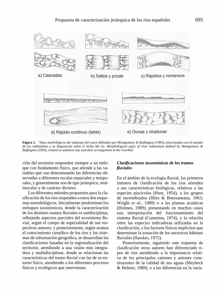
Propuesta de caracterizacion jerarquica de los rıos espanoles 695
Figura 1. Tipos morfologicos del substrato del cauce definidos por Montgomery & Buffington (1993), relacionados con el tamanode los sedimentos y su disposicion sobre el lecho del rıo. Morphological types of river substratum defined by Montgomery &Buffington (1993), related to sediment size and their arrangement in the riverbed.
cion del territorio responden siempre a un enfo-que con fundamento fısico, que atiende a las va-riables que van determinando las diferencias ob-servadas a diferentes escalas espaciales y tempo-rales, y generalmente son de tipo jerarquico, mul-tiescalar y de caracter divisivo.
Los diferentes metodos propuestos para la cla-sificacion de los rıos responden a estos dos esque-mas metodologicos. Inicialmente predominan losenfoques taxonomicos, donde la caracterizacionde los distintos tramos fluviales es unidisciplinar,reflejando aspectos parciales del ecosistema flu-vial, segun el campo de especialidad de sus res-pectivos autores; y posteriormente, segun avanzael conocimiento cientıfico de los rıos y los siste-mas de informacion geografica, se desarrollan lasclasificaciones basadas en la regionalizacion delterritorio, atendiendo a una vision mas integra-dora y multidisciplinar, donde se relacionan lascaracterısticas del tramo fluvial con las de su en-torno fısico, atendiendo a los diferentes procesosfısicos y ecologicos que intervienen.
Clasificaciones taxonomicas de los tramosfluviales
En el ambito de la ecologıa fluvial, los primerosintentos de clasificacion de los rıos atiendena sus caracterısticas biologicas, relativas a lasespecies piscıcolas (Huet, 1954), a los gruposde invertebrados (Illies & Botosaneanu, 1963;Wright et al., 1989) o a las plantas acuaticas(Holmes, 1989), presentando en muchos casosuna interpretacion del funcionamiento delsistema fluvial (Cummins, 1974), y la relacionentre las especies indicadoras utilizadas en laclasificacion, y los factores fısicos implıcitos quedeterminan la zonacion de los sucesivos habitatsfluviales (Hawkes, 1975).
Posteriormente, siguiendo este esquema declasificacion otros autores han diferenciado ti-pos de rıos atendiendo a la importancia relati-va de los principales cationes y aniones cons-tituyentes de la calidad de sus aguas (Meybeck& Helmer, 1989), o a las diferencias en la varia-

696 Gonzalez del Tanago y Garcia de Jalon
bilidad y predictibilidad de su regimen de cau-dales (Poff & Ward, 1989), relacionando dichascaracterısticas con la estructura de las comuni-dades biologicas, y la capacidad de recupera-cion frente a perturbaciones naturales o antropi-cas de los sistemas fluviales (Poff & Ward, 1990).
En el campo de la geomorfologıa fluvial, lostrabajos iniciales de clasificacion tambien sonde tipo taxonomico, centrandose en el reconoci-miento de las diferentes formas del trazado de losrıos. Leopold & Wolman (1957) diferencian trestipos de rıos, rectos, meandriformes y trenzados,proponiendo unos valores umbrales de caudal ypendiente longitudinal para predecir la respuestageomorfologica a cambios en estas variables, yposteriormente Brice (1975) describe tambien eltrazado en planta de los rıos atendiendo a su gra-do de sinuosidad, diferenciando las formas tren-zadas y anastomosadas.
Schumm (1977) resalta la influencia de ladinamica fluvial, y diferencia los rıos controladospor afloramientos rocosos que determinan sumorfologıa, de los rıos aluviales, libres paraajustar sus dimensiones y formas, entre losque distingue los rıos estables, de los rıos conpredominio de erosion o de sedimentacion.
Mas recientemente, Montgomery & Buffing-ton (1993) proponen una clasificacion de los rıosde la costa pacıfica de Washington atendiendo alos procesos fluviales que intervienen a diferentesescalas espaciales. Estos autores definen en estosrıos de montana siete tipos de tramos fluviales,diferenciando por una parte los de origen coluvialo confinados por afloramientos rocosos, de los deorigen aluvial, diferenciando entre estos ultimos,cinco tipos morfologicos distintos segun la es-tructura del substrato, en un esquema de zonacionaltitudinal siguiendo el gradiente de la pendien-te longitudinal y los procesos fluviales asociados(Fig. 1). Adicionalmente, tambien definen los ti-pos de rıos cuya morfologıa queda forzada por lapresencia de restos vegetales.
Finalmente, Rosgen (1994, 1996) proponeuna clasificacion de los rıos basada en diferentesvariables y niveles jerarquicos, que ha tenido unagran aceptacion en el ambito de la restauracionfluvial entre los servicios forestales de EstadosUnidos, ası como una cierta crıtica por parte
de diferentes autores (Kondolf, 1995; Doyle etal., 1999). En un primer nivel de clasificacion,Rosgen diferencia nueve tipos de rıos, de acuerdocon su pendiente longitudinal, sinuosidad yforma de la seccion transversal (Fig. 2). Enun segundo nivel de clasificacion, cada uno deestos siete tipos de rıos, denominados con letrasmayusculas (A, A+, B, C, D, DA, E, F y G) sesubdivide a su vez segun su rango de pendientey granulometrıa del substrato, obteniendo 42subtipos, denominados con numeros y letrasminusculas (A1, A2, B1b, B2c, etc). Un tercernivel de clasificacion alude al estado ecologicodel rıo, descrito en base a su vegetacion riparia,fauna acuatica, regimen de caudales, estabilidadde sus orillas, etc., existiendo un cuarto nivel paraverificar y predecir ciertas variables hidraulicas yde transporte de sedimentos.
Regionalizacion del territorio: Clasificacion delos rıos en el contexto de su cuenca vertien
En 1975, Hynes propone un enfoque integradodel rıo y su entorno, describiendo de forma pio-nera las relaciones existentes entre los procesoshidrologicos del valle y las caracterısticas y fun-cionamiento del ecosistema fluvial.
Los nuevos conceptos relacionando el rıo consu cuenca vertiente, surgidos en base a toda unalınea de investigacion hidrologica en cuencas ex-perimentales (Douglass & Hoover, 1988), faci-litan la propuesta de nuevos enfoques de clasi-ficacion de los rıos, que integran a los sistemasacuaticos en sus sistemas terrestres circundantes.
Los trabajos de Platts (1974) relacionandolas condiciones geomorficas de los rıos con suspoblaciones de salmonidos, y los de Likens et al.(1977) o Borman & Likens (1981) proponiendolas cuencas vertientes pequenas (watersheds)como ecosistemas para el estudio de los ciclos denutrientes y procesos hidrologicos, constituyenantecedentes fundamentales para establecer elmarco conceptual propuesto por Warren (1979)y Lotspeich (1980), en el que consideranla cuenca vertiente como ecosistema basicode clasificacion natural, y Lotspeich & Platts(1982) desarrollan el sistema integrado de

Propuesta de caracterizacion jerarquica de los rıos espanoles 697
Figura 2. Tipos morfologicos de rıos diferenciados por Rosgen (1996) en el Nivel I de su clasificacion. River morphological typesidentified by Rosgen (1996) at the Level I in his classification.
clasificacion para la gestion de los ecosistemasacuaticos y su fauna piscıcola.
En el escenario cientıfico generado portodos estos conceptos, Frissell et al. (1986)proponen un sistema de clasificacion jerarquicade los rıos integrados en su cuenca vertiente,asumiendo un determinismo biologico respectoa los factores fısicos del habitat, los cualesvienen a su vez condicionados sucesivamente,y de forma ascendente, por las caracterısticasdel tramo de rıo, perteneciente a un segmentofluvial, que forma parte de una red de drenaje,que a su vez depende de su cuenca vertiente.Una vez propuesta esta organizacion jerarquica,atendiendo a diferentes escalas geograficas,dichos autores acotan espacialmente los bordeso lımites entre escalas, y clasifican los distintostipos de habitats que pueden existir en cada caso.En este sentido reconocen una “organizacion” dela heterogeneidad de los habitats en el contınuofluvial de Vannote et al. (1980), y consideran laestructura, el desarrollo y la persistencia de cadahabitat como factores ligados al funcionamientohidrologico de la cuenca vertiente, con los cuales
se puede predecir su capacidad o potencial paraalbergar a las diferentes especies.
Este enfoque integrado de organizacionjerarquica de los habitats fluviales propuestopor Frissell et al. (1986) ha sido asimilado enposteriores sistemas de clasificacion de los rıosbasados en procesos fısicos (Montgomery &Buffington, 1997), sirviendo a partir de entoncesde marco conceptual basico para el desarrollode estrategias de gestion y restauracion fluvial(Doppelt et al., 1993; Williams et al.1997, etc.).
Paralelamente a estos trabajos, y con lafinalidad de facilitar la gestion y planificacionde uso multiple en los espacios naturales, sedesarrollan por parte de los Servicios Forestalesde Estados Unidos diferentes propuestas declasificacion de usos y suelos, teniendo encuenta las posibilidades que se vislumbran eneste campo con el desarrollo de la recogidade informacion vıa satelite, y de las tecnicasinformaticas para su analisis (Driscoll et al.,1978), surgiendo una necesidad de unificarcriterios (Nelson et al., 1978), atendiendo a losdiferentes objetivos de planificacion.

698 Gonzalez del Tanago y Garcia de Jalon
Este enfoque de clasificacion del territorio es uti-lizado para definir las ecoregiones de EstadosUnidos, primero por Bailey (1976), el cual propo-ne un sistema de regionalizacion jerarquica, aten-diendo sucesivamente a la influencia del clima, lavegetacion natural potencial, los suelos y la for-mas del relieve; y posteriormente por Omernik(1987), este ultimo con una finalidad enfocada ala gestion de la calidad de las aguas de los ecosis-temas acuaticos, haciendo especial hincapie en lainfluencia del uso del suelo.
Las diferentes propuestas de ecoregiones soncontrastadas posteriormente por sus respectivosautores (Bailey, 1983; 1995; Omernik 1995), in-tegrando en sucesivas publicaciones los concep-tos del rıo y su cuenca vertiente, en un territorioconfigurado por diferentes factores, que incidena distinta escala espacial y temporal (Omernik &Bailey, 1997; Griffith et al., 1999).
Mas recientemente, la necesidad de generali-zar los sistemas de gestion y planificacion de losecosistemas acuaticos, junto al desarrollo de lossistemas de informacion geografica y la disponi-bilidad de cartografıa digitalizada para el estudiode grandes cuencas, ha propiciado el desarrollode numerosos estudios, donde se analiza la rela-cion entre las distintas clasificaciones del territo-rio segun ecoregiones y cuencas vertientes, y lascaracterısticas biologicas de los respectivos eco-sistemas acuaticos (Hawkins & Norris, 2000).
En este sentido, (Hawkins et al., 2000) lle-gan a la conclusion de que las regionalizaciones agran escala (ej. ecoregiones) absorben una parterelativamente pequena de la variabilidad biologi-ca y son de uso limitado en el campo de los in-dicadores biologicos, como ya destacaron en sudıa Omernik & Bailey (1997), mientras que tie-nen un interes notable en la estratificacion inicialdel territorio para seleccionar las localidades deestudio a pequena escala, asegurando una repre-sentacion completa de las distintas condicionesambientales existentes.
Hoy dıa es indudable el interes de utilizar re-gionalizaciones del territorio a diferentes escalaspara la clasificacion de los ecosistemas acuaticos,dada la facilidad de disponer de informacion yherramientas adecuadas para ello, que permitenreconocer los distintos flujos y dimensiones del
Tabla 1. Sistema A de clasificacion de los rıos segun laDirectiva Marco del Agua. System A for river classificationaccording to the Water Framework Directive.
Tipologıa Descriptores
Ecoregion Ecoregiones (ver mapa A en Annexo XI)Tipo Altitud
• Zonas Altas: > 800 m• Altitud Media: 200 to 800 m• Zonas bajas: < 200 mTamano de la cuenca vertiente
• Pequena: 10 a 100 km2
• Media: > 100 a 1000 km2
• Grande: > 1000 a 10 000 km2
• Muy grande: > 10 000 km2
Geologıa• Caliza• Silıcea• Organica
sistema fluvial (Amoros & Petts, 1993), ası comointerpretar la influencia de los principales facto-res que determinan su funcionamiento ecologi-co a diferentes escalas espacio-temporales, decaracter natural o antropico (Robertson & Saad,2003; Detenbeck et al., 2004).
Sin restar interes a las clasificaciones detipo taxonomico, equivalentes a modelos de“caja negra” donde la confluencia de atributospermite agrupar a los objetos clasificados,para posteriormente interpretar los grupos oclases obtenidas, creemos que hoy dıa son lasclasificaciones basadas en la regionalizacion delterritorio, y en el conocimiento de la dependenciahidrologica y ecologica del rıo respecto asu entorno, las que permiten caracterizar conmayor base fisica y ecologica los distintos tiposde sistemas y habitats fluviales, facilitando almismo tiempo su gestion y planificacion deacuerdo a los diferentes tipos de estructura y defuncionamiento.
La clasificacion de los rıos en la DirectivaMarco del Agua
La Directiva Marco del Agua establece como eta-pa inicial para su implementacion, la clasifica-cion de las aguas superficiales atendiendo a lossiguientes tipos de masas de agua:
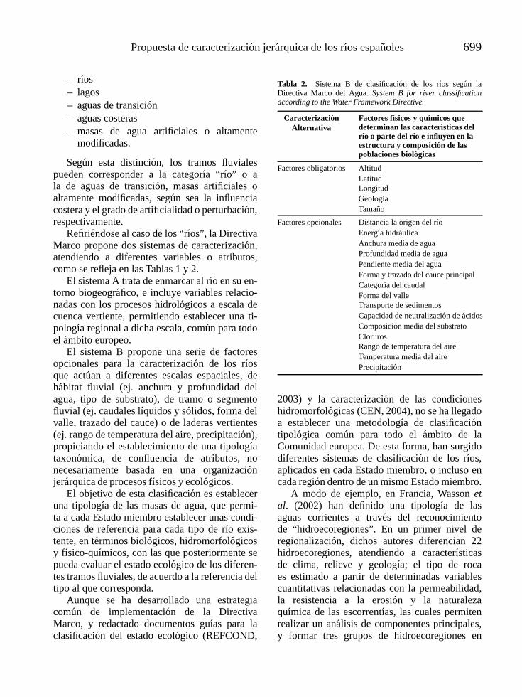
Propuesta de caracterizacion jerarquica de los rıos espanoles 699
– rıos– lagos– aguas de transicion– aguas costeras– masas de agua artificiales o altamente
modificadas.
Segun esta distincion, los tramos fluvialespueden corresponder a la categorıa “rıo” o ala de aguas de transicion, masas artificiales oaltamente modificadas, segun sea la influenciacostera y el grado de artificialidad o perturbacion,respectivamente.
Refiriendose al caso de los “rıos”, la DirectivaMarco propone dos sistemas de caracterizacion,atendiendo a diferentes variables o atributos,como se refleja en las Tablas 1 y 2.
El sistema A trata de enmarcar al rıo en su en-torno biogeografico, e incluye variables relacio-nadas con los procesos hidrologicos a escala decuenca vertiente, permitiendo establecer una ti-pologıa regional a dicha escala, comun para todoel ambito europeo.
El sistema B propone una serie de factoresopcionales para la caracterizacion de los rıosque actuan a diferentes escalas espaciales, dehabitat fluvial (ej. anchura y profundidad delagua, tipo de substrato), de tramo o segmentofluvial (ej. caudales lıquidos y solidos, forma delvalle, trazado del cauce) o de laderas vertientes(ej. rango de temperatura del aire, precipitacion),propiciando el establecimiento de una tipologıataxonomica, de confluencia de atributos, nonecesariamente basada en una organizacionjerarquica de procesos fısicos y ecologicos.
El objetivo de esta clasificacion es estableceruna tipologıa de las masas de agua, que permi-ta a cada Estado miembro establecer unas condi-ciones de referencia para cada tipo de rıo exis-tente, en terminos biologicos, hidromorfologicosy fısico-quımicos, con las que posteriormente sepueda evaluar el estado ecologico de los diferen-tes tramos fluviales, de acuerdo a la referencia deltipo al que corresponda.
Aunque se ha desarrollado una estrategiacomun de implementacion de la DirectivaMarco, y redactado documentos guıas para laclasificacion del estado ecologico (REFCOND,
Tabla 2. Sistema B de clasificacion de los rıos segun laDirectiva Marco del Agua. System B for river classificationaccording to the Water Framework Directive.
CaracterizacionAlternativa
Factores fısicos y quımicos quedeterminan las caracterısticas delrıo o parte del rıo e influyen en laestructura y composicion de laspoblaciones biologicas
Factores obligatorios AltitudLatitudLongitudGeologıaTamano
Factores opcionales Distancia la origen del rıoEnergıa hidraulicaAnchura media de aguaProfundidad media de aguaPendiente media del aguaForma y trazado del cauce principalCategorıa del caudalForma del valleTransporte de sedimentosCapacidad de neutralizacion de acidosComposicion media del substratoClorurosRango de temperatura del aireTemperatura media del airePrecipitacion
2003) y la caracterizacion de las condicioneshidromorfologicas (CEN, 2004), no se ha llegadoa establecer una metodologıa de clasificaciontipologica comun para todo el ambito de laComunidad europea. De esta forma, han surgidodiferentes sistemas de clasificacion de los rıos,aplicados en cada Estado miembro, o incluso encada region dentro de un mismo Estado miembro.
A modo de ejemplo, en Francia, Wasson etal. (2002) han definido una tipologıa de lasaguas corrientes a traves del reconocimientode “hidroecoregiones”. En un primer nivel deregionalizacion, dichos autores diferencian 22hidroecoregiones, atendiendo a caracterısticasde clima, relieve y geologıa; el tipo de rocaes estimado a partir de determinadas variablescuantitativas relacionadas con la permeabilidad,la resistencia a la erosion y la naturalezaquımica de las escorrentıas, las cuales permitenrealizar un analisis de componentes principales,y formar tres grupos de hidroecoregiones en
700 Gonzalez del Tanago y Garcia de Jalon
base a estas variables geologicas. El relieve esestimado a partir de tres variables, la altitud,la pendiente del terreno y la pendiente dela lınea que une los puntos mas bajos delcauce (thalweg), para las que se han definidounos rangos de valores y definido distintasclases de altitud y pendiente, respectivamente.Y finalmente, el clima se ha analizado atraves de cuatro variables, la precipitacion anual,las precipitaciones maximas en 24 horas, lavariacion estacional de precipitaciones y latemperatura maxima media del mes de Julio,respecto a las cuales tambien se han definido unasclases en relacion al rango de valores absolutos yrelativos de dichas variables.
En un segundo nivel de regionalizacion,dentro de cada una de estas 22 hidroecoregionesse ha estudiado la posibilidad de diferenciardistintas subregiones en base a condicioneslocales de tipo geologico o climatico, facilitandosu agrupacion geografica.
En Holanda han definido una serie de “tiposde rıos” atendiendo a la pendiente del caucey velocidad de las aguas, geologıa y superficiede cuenca vertiente, para cuyo reconocimientose disena una clave taxonomica donde aparecensucesivamente los rangos de valores establecidospara estas variables. De forma similar, enChipre se ha propuesto una tipologıa de rıosque diferencia en primer lugar el origen delas aguas y la pendiente longitudinal delcauce, posteriormente la naturaleza geologica,a continuacion la superficie vertiente y laprecipitacion, y finalmente el tipo de regimen,permanente o efımero, considerando, a cada niveltaxonomico de clasificacion, distintos rangos devalores de las variables consideradas.
En Espana tambien se han propuesto distintosmetodos para la tipologıa de los rıos atendiendoa la Directiva Marco. Ası, Bonada et al. (2002),a partir del sistema B de clasificacion de laDirectiva Marco, proponen una tipologıa de lascuencas mediterraneas analizadas en el proyectoGUADALMED en la que se diferencian 6ecotipos, atendiendo al tamano de rıo (grande,mediano, pequeno, rambla), geologıa de lacuenca (silıcea, calcarea o sedimentaria), yposicion (tramo de cabecera, medio-bajo y bajo).
La clasificacion obtenida por estos autores resultaexcesivamente simplificada, de tipo taxonomico,donde en cada una de las clases obtenidaspuede haber una gran diversidad de condicionesecologicas, sin que a nuestro entender pueda serutil para establecer las condiciones de referencia,biologicas e hidromorfologicas, respectivas paracada clase establecida.
Con mas precision hidrologica, la AgenciaCatalana del Agua (ACA, 2002) ha diferencia-do 5 regiones fluviales y 10 subregiones de ges-tion fluvial, atendiendo a criterios hidrologicos ygeologicos. Para su reconocimiento se estableceuna clave taxonomica, donde los criterios utiliza-dos no estan organizados de forma jerarquica, enbase a procesos fısicos o hidrologicos.
Ollero et al. (2003) han propuesto una clasifi-cacion de los rıos de Aragon atendiendo a sus ca-racterısticas geomorfologicas, donde se conside-ran variables topograficas, hidroclimaticas y mor-fologicas, siguiendo un esquema jerarquico en elque se reconocen la escala de ecoregion (caracte-rizada por la altitud y la localizacion geografica)y la del segmento fluvial (atendiendo a la formadel valle y el caudal especıfico). Esta tipologıa delos rıos aragoneses responde a los procesos fısi-cos que configuran la morfologıa de los distintostramos de rıos, pero no incluye algunas variablescomo el regimen de caudales y el tipo de substra-to, que pueden influir notablemente en las carac-terısticas ecologicas de cada tramo.
Finalmente, el Centro de Estudios Hidrografi-cos (CEDEX, 2004) ha establecido una caracte-rizacion de los rıos espanoles diferenciando 29tipos ambientales, que han sido obtenidos me-diante una clasificacion divisiva en base al cau-dal medio anual, pendiente media de la cuenca,altitud, conductividad de las aguas, temperaturamedia anual y orden del rıo. Inicialmente se hanconsiderado tres regiones distintas, la region me-diterranea, la region atlantica (euosiberiana) y laregion macaronesica, y en cada una de ellas se haprocedido a la clasificacion divisiva de los cursosde agua atendiendo a las variables mencionadas,si bien en un orden de consideracion distinto encada una de ellas.
El analisis conjunto de los distintos sistemaspropuestos hasta la fecha para la caracterizacion

Propuesta de caracterizacion jerarquica de los rıos espanoles 701
Figura 3. Esquema de caracterizacion jerarquica de los rıos, atendiendo a la dependencia asimetrica de los factores que determinansus comunidades biologicas. Hierarchical river characterization scheme, according to the asymetrical dependence of main factorsdetermining biological communities.
de los rıos como fase inicial de la implementa-cion de la Directiva Marco, permite obtener al-gunas conclusiones, como sigue:
– La mayorıa de las tipologıas propuestas deri-van de analisis estadısticos realizados a par-tir de una serie de datos disponibles, distintossegun las zonas estudiadas, relativos a varia-bles que tienen un nivel de significacion hi-drologica y ecologica muy diferente. Con ellose obtienen clasificaciones de tipo taxonomi-co, de escala unica, donde se consideran multi-ples factores siguiendo un modelo de “caja ne-gra” o gris, que no responde a una ordenacionjerarquica previa de dichos factores, basada enel conocimiento cientıfico de su influencia enlos ecosistemas fluviales.
– En general, las clasificaciones obtenidasno responden a una interpretacion de losprocesos fısicos e hidrologicos que actuana diferentes escalas espaciales y temporalesen el ecosistema fluvial, ni parten de unplanteamiento ecologico de reconocimiento dediscontinuidades, o elementos de clasificacion,en el contınuo fluvial.
– Los resultados obtenidos hasta la fecha no pa-recen muy satisfactorios a la hora de poder es-tablecer comparaciones entre los distintos ti-pos establecidos en relacion a sus caracterısti-cas fısicas, puesto que en muchos casos se de-finen en base a distintas variables, y por con-siguiente, tampoco facilitan la comparacionen relacion a sus caracterısticas biologicas.
– La denominacion de los grupos de rıos obteni-dos alude a las variables utilizadas para su ob-tencion, y no facilita su localizacion geografi-ca, agrupando en muchos casos tramos fluvialesde diferentes regiones o distritos hidrograficos.
PROPUESTA DE CLASIFICACIONJERARQUICA DE LOS RIOSESPANOLES
La tipologıa que se propone para la caracteriza-cion de los rıos espanoles de acuerdo con losobjetivos de la Directiva Marco del Agua, partedel reconocimiento de la dependencia jerarqui-ca que mantienen los distintos factores quedeterminan la estructura y funcionamiento de
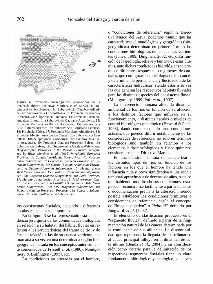
702 Gonzalez del Tanago y Garcia de Jalon
Figura 4. Provincias biogeograficas reconocidas en laPenınsula Iberica por Rivas Martınez et al. (2002). 4: Pro-vincia Atlantica Europea. 4a: Subprovincia Cantabro-Atlanti-ca; 4b: Subprovincia Orocantabrica. 7: Provincia Cevenense-Pirenaica. 7a: Subprovincia Pirenaica. 14: Provincia Lusitano-Andaluza-Litoral. 14a Subprovincia Gaditano-Algarviense. 15:Provincia Mediterranea Iberica Occidendal. 15a SubprovinciaLuso-Extremadurense; 15b Subprovincia Carpetano-Leonesa.16: Provincia Betica. 17: Provincia Murciano-Almeriense. 18:Provincia Mediterranea Iberica Central. 18a Subprovincia Cas-tellana. 18b Subprovincia Oroiberica: 18c: Subprovincia Ba-jo Aragonesa. 19: Provincia Catalana-Provenzal-Balear. 19aSubprovincia Balear; 19b: Subprovincia Catalana-Valenciana.Biogeographic Provinces in the Iberian Peninsula recogni-zed by Rivas Martınez et al. (2002).4: Atlantic EuropeanProvince. 4a Cantabrian-Atlantic Subprovince; 4b: Orocan-tabric Subprovince. 7: Cevenense-Pyrenean Province. 7a Py-renean Subprovince. 14: Coastal Lusitan-Andalusian Provin-ce. 14a Gaditan-Algarvian Subprovince. 15: MediterraneanWest Iberian Province. 15a Lusitan-Extremadurean Subprovin-ce; 15b: Carpetan-Leonese Subprovince. 16: Betic Province.17: Murcian-Almeriensian Province. 18: Mediterranean Cen-tral Iberian Province. 18a Castillian Subprovince; 18b: Oroi-berian Subprovince: 18c: Low Aragonese Subprovince. 19:Balearic-Catalan-Provencal Province. 19a Balearic Subpro-vince. 19b: Catalan-Valencian Subprovince.
los ecosistemas fluviales, actuando a diferentesescalas espaciales y temporales.
En la figura 3 se ha representado esta depen-dencia jerarquica de las comunidades biologicasen relacion a su habitat, del habitat fluvial en re-lacion a las caracterısticas del tramo de rıo, y deeste en relacion a las de su cuenca vertiente, en-marcada a su vez en una determinada region bio-geografica, basada en los conceptos anteriormen-te comentados de Frissell et al. (1986); Montgo-mery & Buffington (1993), etc.
En condiciones no alteradas por el hombre,
o “condiciones de referencia” segun la Direc-tiva Marco del Agua, podemos asumir que lascaracterısticas climatologicas y geograficas (bio-geograficas) determinan en primer termino lascondiciones hidrologicas de las cuencas vertien-tes (Jones, 1999; Dingman, 2002, etc.). En fun-cion de la geologıa, relieve y tamano de estas ulti-mas, ante dichas condiciones hidrologicas se pro-ducen diferentes respuestas o regımenes de cau-dales, que configuran la morfologıa de los caucesy determinan la permanencia y fluctuacion de lascaracterısticas hidraulicas, siendo estas a su vezlas que generan los respectivos habitats fluvialespara las distintas especies del ecosistema fluvial(Montgomery, 1999; Poff et al., 1997)
La intervencion humana altera la dinamicaambiental de los rıos en funcion de su afecciona los distintos factores que influyen en sufuncionamiento, a distintas escalas o niveles decontrol hidrologico y ecologico (Bravard & Petts,1993), dando como resultado unas condicionesactuales que pueden diferir notablemente de lasconsideradas de referencia, no solo en terminosbiologicos sino tambien en relacion a loselementos hidromorfologicos y fısico-quımicosconsiderados en la Directiva Marco.
En esta ocasion, se trata de caracterizar alos distintos tipos de rıos en funcion de losfactores en los que el hombre ha tenido unainfluencia nula o poco significativa a una escalatemporal aproximada de decenas de anos, o en losque habiendo modificado sus condiciones, estaspueden reconstruirse facilmente a partir de datoso documentacion previa a la alteracion, siendoposible establecer las condiciones primitivas oconsideradas de referencia, segun el conceptode “imagen objetivo” o “leitbild” definido porJungwirth et al. (2002).
El elemento de clasificacion propuesto es el“segmento fluvial”, definido a partir de la frag-mentacion natural de los cauces determinada porla confluencia de sus afluentes. La discontinui-dad que representa la llegada de los tributariosal cauce principal influye en la dinamica de es-te ultimo (Benda et al., 2004), y su considera-cion como criterio para la delimitacion de losrespectivos segmentos fluviales tiene un clarofundamento hidrologico y ecologico, a la vez

Propuesta de caracterizacion jerarquica de los rıos espanoles 703
Tabla 3. Clasificacion jerarquica de los habitats fluviales, incluyendo los factores y criterios de caracterizacion a diferentes escalas.Hierarchical classification of river habitats, including the factors and characterisation criteria at different spatial scales.
EcoregionProvincias biogeograficas
Subprovincias biogeograficasCuenca vertiente
TamanoMuy pequena (< 10 km2)Pequena (10-100 km2)Mediana (100-1000 km2)Grande (1000-10 000 km2)Muy grande (10 000-25 000 km2)Gran arteria fluvial (> 25 000 km2)
GeologıaSilıceaCalizaArcillosa
Segmento fluvialTipo geomorfologico (adaptado de Rosgen, 1996)
Arroyo o torrente de alta montana (Aa+)Rıo de montana (A)Tramos altos y de piedemonte (B)Tramos trenzados (D)Tramos anastomosados (DA)Tramos meandriformes (E)Hoces y Canones angostos (F), Tramos encajonados (G)
Regimen de caudalesPermanente
Dependiendo del regimen de precipitacionesNivalNivopluvialPluvionivalPluvial
Dependiendo de la presencia de acuıferosNo permanente
EfımeroTemporal
Por agotamiento de escorrentıas Por infiltracion de escorrentıasHabitat fluvial
Granulometrıa del substratoCohesivo
RocaArcilla
No cohesivo: Aluvial (adaptado de Montgomery y Buffington, 1997)En cascadaEscalonesRapido contınuoRapidos y remansosArenas con dunas y rizadurasBarras e islas
VegetacionComunidades arboreas y arbustivasMacrofitas emergentes de orillaVegetacion acuatica
Otras caracterısticasSubstrato de travertinosFormaciones karsticasYesosAguas salinas

704 Gonzalez del Tanago y Garcia de Jalon
que facilita la diferenciacion objetiva de losmismos sobre la cartografıa.
Una vez reconocidos los segmentos fluviales,en una disminucion de escala espacial (up-scaling) se considera la cuenca vertiente alextremo inferior del segmento, y posteriormentela region biogeografica a la que correspondedicha cuenca. Dentro de cada segmento, yaumentando la escala espacial (down-scaling), seconsideran diferentes unidades funcionales queatienden a discontinuidades fısicas, en las que sereconocen a su vez diferentes tipos de habitatsfluviales, sobre los que se pueden analizar lascomunidades biologicas.
En la Tabla 3 se presenta la caracterizacion je-rarquica propuesta, incluyendo los diferentes ni-veles de clasificacion y los criterios utilizados pa-ra las diferentes escalas espaciales consideradas.
Ecoregion: Provincias biogeograficas
El reconocimiento de ecoregiones, caracterizadaspor factores naturales que actuan a gran escala,es la mejor manera de iniciar la regionalizacionde un territorio, tratando de definir areasecologicamente homogeneas donde llevar acabo planes de gestion y conservacion de lossistemas naturales (Omernik & Bailey, 1997).Esta consideracion de ecoregiones, propuesta enel sistema A de clasificacion de la DirectivaMarco, esta siendo aplicada en varios paıses, parala elaboracion de su respectiva tipologıa fluvial(Wasson et al., 2002; Brilly et al., 2004).
En Espana existe una gran experiencia en estetipo de regionalizacion del territorio espanol, ba-sada fundamentalmente en los trabajos de RivasMartınez y colaboradores (Rivas Martınez, 1987;Rivas Martınez et al., 2002), que representa unagran ayuda para integrar la influencia conjunta defactores como el clima, la geologıa y el relieveen las condiciones hidrologicas de las respectivascuencas vertientes.
En la figura 4 aparecen representadas lasProvincias biogeograficas reconocidas por dichosautores en la Penınsula Iberica, cuya utilizacionnos parece de gran interes a la hora deestablecer la tipologıa de los rıos espanoles,dado que en su diferenciacion se han tenido
Tabla 4. Superficie de cuenca espanola de los principales rıosde la Penınsula Iberica. Spanish basin area for the main riversof the Iberian Peninsula.
Rıo Area vertiente(km2)
Nervion (Paıs Vasco) 0 1764Ter (Cataluna) 0 3011Guadalhorce (Sur) 0 3158Nalon (Asturias) 0 4866Llobregat (Cataluna) 0 4948Sil (Galicia) 0 7982Mino (Galicia) 16 212Segura 19 120Jucar 42 900Tajo 55 810Guadiana 60 210Guadalquivir 63 240Duero 78 960Ebro 85 560
en cuenta caracterısticas termo-pluviometricas,de altitud y pendiente de las laderas, geologıay suelos, situacion geografica, etc., muchas deellas relacionadas con algunos de los descrip-tores opcionales que incluye el sistema B declasificacion propuesto por la Directiva Marco.
La nomenclatura de estas provincias bio-geograficas alude a su ubicacion geografica y fa-cilita considerablemente la localizacion de losrespectivos rıos y segmentos fluviales, hecho queanteriormente ya ha sido considerado de gran in-teres en la Directiva Europea de Habitat, dondese ha seguido un esquema de regionalizacion si-milar para la gestion y conservacion de los res-pectivos habitats (Rodwell et al., 1997).
Cuenca vertiente
Hidrologicamente, el territorio se organiza encuencas vertientes, cuyas caracterısticas defuncionamiento y respuesta estan condicionadaspor la region biogeografica en la que se enmarcan(Omernik y Griffith, 1991).
Ante similares condiciones climatologicas,la respuesta hidrologica de cada cuen-ca depende, entre otros factores, de sutamano, determinando el area de captacion deprecipitaciones y superficie donde se generan lasescorrentıas, y de su geologıa, condicionando lascaracterısticas de infiltracion y retencion de aguaen el interior de la cuenca (Black, 1997).

Propuesta de caracterizacion jerarquica de los rıos espanoles 705
Son estas caracterısticas de tamano y geologıalas que propone la Directiva Marco para llevar acabo la tipologıa fluvial, y sobre las que propo-nemos las categorıas que aparecen en la Tabla 3.
La Directiva Marco del Agua estableceuna clase unica de cuencas “muy grandes”,con superficie mayor de 10 000 km2. Dada laamplitud del rango de superficies que podemosencontrar en esta clase dentro del ambitoeuropeo, y reconociendo diferencias ecologicasque pueden existir atendiendo a la magnitudde los caudales y su predictibilidad (Tabla4) proponemos la diferenciacion de una claseadicional para los tramos bajos de las grandesarterias fluviales, con una superficie vertientesuperior a 25 000 km2.
Figura 5. Mapa de las litologıas dominantes en la PenınsulaIberica elaborado por Gutierrez Elorza (1994). Map of thedominant lithologies in the Iberian Peninsula proposed byGutierrez Elorza (1994).
Para la caracterizacion de la geologıa delas cuencas vertientes, y tratando de sim-plificar la informacion suministrada por lasdiferentes cartografıas existentes en nuestropaıs, proponemos la utilizacion del trabajode Gutierrez Elorza (1994), donde se reco-nocen las categorıas silıcea, caliza y arci-llosa, segun se representa en la figura 5.
La Directiva Marco incluye una clase geologi-ca “organica” que nosotros no hemos tenido en
cuenta, considerando la escasez de su represen-tacion en la Penınsula Iberica. Por el contra-rio, consideramos que existe una gran superfi-cie cubierta por materiales sedimentarios de ti-po arcilloso, recubriendo gran parte de las dosMesetas y las depresiones de las cuencas medi-terraneas, y que es interesante destacar esta cate-gorıa no recogida en la Directiva Marco, teniendoen cuenta su influencia en la morfologıa y tipo desubstrato de los cauces.La adscripcion de cada cuenca a una u otra ca-tegorıa geologica dependera del porcentaje queexista de cada una de ellas, surgiendo a menudocategorıas intermedias a partir de las cuencas detamano medio, que pueden quedar caracterizadasa su vez como subclases, dentro de una mismacategorıa geologica.
Segmento fluvial
Considerando la confluencia de afluentes comofactor de discontinuidad hidrologica en los res-pectivos cauces principales, proponemos utilizarlos segmentos fluviales identificados por la admi-nistracion publica espanola (MOP, 1965) para laelaboracion de su tipologıa.
En el trabajo citado, cada rıo es codificadomediante dıgitos, y definido en su longitud y areavertiente en cada uno de los segmentos fluvialesque van surgiendo entre confluencias.
Se trata de un estudio basico y de referencia,que ofrece un criterio fisico y “objetivo”de identificacion de los segmentos fluviales,facilmente aplicable sobre cartografıa y confundamento hidrologico y ecologico.
Cada segmento ası reconocido es posterior-mente caracterizado en funcion de su regimen decaudales y sus condiciones geomorfologicas, am-bos relacionados con la magnitud del flujo circu-lante y la superficie vertiente, que se ven incre-mentados sucesivamente, despues de la llegadade cada afluente.
En relacion a la caracterizacion del regimende caudales, y teniendo en cuenta los trabajos dePoff & Ward (1989) y Olden & Poff (2003), he-mos diferenciado en primer termino los regıme-nes permanentes, con caudal circulante todo elano, de los regımenes no permanentes, conside-

706 Gonzalez del Tanago y Garcia de Jalon
rando la “temporalidad” de los caudales comouno de los factores principales que condicionael funcionamiento del ecosistema fluvial. Poste-riormente, dentro de cada tipo de regimen he-mos considerado su “predictibilidad” y “variabi-lidad”, atendiendo al origen principal de las es-correntıas, predecibles pero con oscilaciones es-tacionales en el caso de responder al regimende precipitaciones, mas homogeneas en el casode afluencia de aguas subterraneas, y de caractermas torrencial en el caso de los regımenes efıme-ros, localizados principalmente en las ramblas.
Para la caracterizacion de las condicionesgeomorfologicas de cada segmento fluvial propo-nemos adaptar la clasificacion de Rosgen (1996),considerando los 9 tipos morfologicos que Ros-gen reconoce en el primer nivel de su clasifi-cacion, basados en la pendiente longitudinal delcauce, el coeficiente de sinuosidad y la forma do-minante de la seccion transversal (Fig. 2).
En este sentido, y con el fin de poder asignarun tipo morfologico dominante a cada segmentofluvial en base a la cartografıa, proponemosasignar los distintos tipos morfologicos enfuncion de los valores de pendiente longitudinal,coeficiente de sinuosidad, y tipo de valle, segunsu grado de encajonamiento.
Tramo o Sector fluvial
Finalmente, dentro de cada segmento fluvial sereconocen diferentes sectores o tramos donde lascaracterısticas de substrato, forma de las orillas,estabilidad del cauce, etc., pueden ser diferentes,configurando distintos tipos de habitats fluviales.
Para la caracterizacion de los distintos secto-res es necesario realizar un reconocimiento decampo en cada segmento fluvial, tras el cual sepueda detallar, en una escala cada vez mayor, lascondiciones hidromorfologicas en que se desa-rrollan las respectivas comunidades biologicas.
La granulometrıa y organizacion de las dis-tintas formas del lecho determinan importantesaspectos del habitat fluvial, estando determina-das por las variables hidraulicas que establecenlos caudales circulantes, sobre un cauce no rıgido(Hey, 1997). Para su caracterizacion hemos dife-renciado en primer termino, siguiendo a Schumm
(1977), el tipo de material cohesivo, de roca o ar-cilla, del no cohesivo, referido al material trans-portado y seleccionado por la accion de la co-rriente (substrato aluvial).
Respecto al substrato no cohesivo, de gravasy arenas, las distintas formas del lecho quepueden organizarse en cada caso han sidodescritas con detalle por Church (1992) yMontgomery & Buffington (1997). En lossectores de cabecera de alta montana, ellecho de los rıos y arroyos esta constituidopor grandes bloques de origen coluvial, quedeterminan la formacion de “cascadas”. Haciaaguas abajo, el tamano medio de estos bloquesdisminuye, y la corriente es capaz de organizarpequenos “escalones”, donde se reconoce unaalternancia de pozas y pequenos saltos queafectan respectivamente a toda la secciontransversal, todavıa de pequena anchura. Segundisminuye la pendiente longitudinal, hacia aguasabajo se forman tramos de “rapidos contınuos”,con gravas y cantos rodados, desapareciendo laspequenas presas organizadas por las piedras demayor tamano que constituıan los escalones deaguas arriba. Finalmente, hacia aguas abajo, yen funcion de un tamano menor de los cantosrodados y abundancia de gravas, se organiza unaalternancia de “rapidos y remansos”, en la quese reconoce, sobre una anchura de cauce mayor,una variacion transversal de las condicioneshidraulicas entre las dos orillas (Fig. 1).
En relacion al substrato no cohesivo de arenas,son conocidas las formas del lecho que puedenestablecerse en funcion de la energıa hidraulicade la corriente, con “rizaduras” y “dunas” aliniciarse el movimiento de las partıculas conuna energıa hidraulica menor, un “lecho liso”en la fase de transicion o movimiento crıtico,y la formacion de “antidunas” en los casosde elevada potencia hidraulica y movimientosupercrıtico (Chang, 1988).
El reconocimiento de los segmentos fluvialescon multiples cauces puede detallarse en funcionde la forma de las islas, el grado de ramificacionde los canales, etc. segun se detalla en el trabajode Thorne (1997).
La vegetacion de las riberas, su composiciony estructura, cobertura, continuidad, etc., son

Propuesta de caracterizacion jerarquica de los rıos espanoles 707
aspectos fundamentales del ecosistema fluvial,que han sido incluidos en la Directiva Marcocomo elementos hidromorfologicos indicadoresdel estado ecologico de los rıos (CEN, 2004).
En la aplicacion de la Directiva, se trata devalorar las condiciones actuales de la vegetacionriparia en los distintos tramos fluviales, en re-lacion a las comunidades que deberıan existiren la zona, consideradas como referencia. Porello proponemos describir la vegetacion ripariacon el mayor detalle posible, en relacion a laformacion vegetal dominante en las orillas, enlas riberas (en sentido estricto) y en la llanu-ra de inundacion, aludiendo a su grado de co-bertura, composicion especıfica y continuidad,siguiendo un enfoque similar al propuesto porWinward (2000), con la informacion de refe-rencia suministrada por Garilleti y Lara (2002).
La aplicacion de ındices como el QBR(Munne et al.,1998) facilita la valoracion com-parativa del estado ambiental de las riberas, pe-ro no deberıa utilizarse en la implementacion dela Directiva Marco, donde el objetivo no es tan-to establecer una ordenacion de “mejor a peor”en funcion de un valor obtenido con el ındi-ce, sino de reconocer la similitud o diferenciaentre las condiciones actuales y las de referen-cia de cada zona, en terminos de composicion ydinamica de las respectivas formaciones vegeta-les, que en algunos casos podrıan ser muy dife-rentes del esquema de valoracion unica implıcitoen el mencionado ındice.
Otras caracterısticas
Finalmente, cada tramo o sector fluvial puedeparticularizarse en funcion de factores limitan-tes locales, relativos al tipo de substrato (traver-tinos, formaciones karsticas, etc.), presencia degeologıas especıficas (yesos, salinas, aguas ter-males, etc.) u otros factores que pueden conside-rarse de interes para caracterizar las condicionesdel habitat en el que se desarrollan las respectivascomunidades biologicas peculiares.
APLICACION DEL ESQUEMA DECARACTERIZACION JERARQUICAPROPUESTO Y CLASIFICACION DELOS SEGMENTOS FLUVIALES
El esquema de caracterizacion jerarquica pro-puesto puede aplicarse directamente a todo elambito de la Penınsula Iberica, o por grandes re-giones hidrograficas (actuales unidades de plani-ficacion hidrologica), y esta preparado para serdefinido mediante programas informaticos (Arc-Gis 8.3), con los cuales se pueden obtener distin-tas cartografıas, a la escala espacial o de nivel decaracterizacion deseados.
Se trata de un metodo de caracterizacion detoda la red de drenaje considerada sencillo yfacilmente abordable en la actualidad, de tipo ar-borescente, donde cada segmento fluvial quedacaracterizado por su localizacion geografica (pro-vincia y subprovincia biogeografica), atributos desu cuenca vertiente (tamano y geologıa) y carac-terısticas hidrologicas (regimen de caudales) ygeomorfologicas (tipo de cauce) que determinansus habitats fluviales (granulometrıa del substra-to, formas del lecho, orillas, riberas, etc.).
La posibilidad de incorporar de forma gene-ral, o individual para un determinado grupo derıos o segmentos fluviales, cualquier informa-cion adicional que se considere de interes pa-ra detallar uno o varios de los factores consi-derados, permite incluir todos los datos com-plementarios que estan disponibles en algunasde las regiones hidrograficas, o pueden estar-lo gradualmente en un futuro, en una estructu-ra de datos comun a todo el territorio espanol,siendo un sistema de caracterizacion abierto ydinamico, en el sentido de aceptar nueva infor-macion sin modificar su base conceptual inicial.
Una vez completada la “caracterizacion” de lared de drenaje se puede proceder a la “clasifica-cion” de los respectivos segmentos fluviales, me-diante la ordenacion jerarquica de los tramos flu-viales considerados y la identificacion de tipos derıos homogeneos. En este caso, son los atributos
708 Gonzalez del Tanago y Garcia de Jalon
de la cuenca vertiente (tamano y geologıa) y tipode regimen de caudales los factores que puedenfacilitar en mayor medida la identificacion de ti-pos o “clases” de rıos, pudiendo surgir dentro decada clase diferentes “subclases”, en funcion deltipo geomorfologico y substrato del cauce, de sulocalizacion geografica (provincia y subprovinciabiogeografica), o de cualquier otro factor existen-te en la zona de estudio, atendiendo siempre almismo esquema comun de caracterizacion y des-cripcion de las caracterısticas fluviales, con basehidrologica y ecologica.
No todas las posibles combinaciones de losfactores utilizados en la caracterizacion propuestaexisten en condiciones naturales, al estar algunosde estos factores correlacionados entre sı (ej. regionbiogeografica con geologıa y regimen de caudales;morfologıa del segmento fluvial con estructuradel substrato, etc.). No obstante, las condicionesactuales pueden diferir de las naturales, y se puedenencontrar combinaciones de factores distintas alas esperadas. En este caso, el esquema decaracterizacion propuesto ayuda a interpretar lasalteraciones debidas a intervenciones humanas,ofreciendo las pautas naturales geomorfologicas ehidrologicas que deben corresponder a cada una delas regionesy tipologıasestablecidas.
El numero de grupos o clases de rıos quepuede obtenerse finalmente en cada caso de-pendera de la heterogeneidad ecologica de ca-da region, no debiendo tratar de reducir excesi-vamente dicho numero, teniendo en cuenta queel territorio espanol es muy diverso en termi-nos ambientales, y que necesariamente hemos deencontrar un numero de tipos de rıos diferen-tes mucho mayor que otras regiones europeas.
Finalmente, este esquema de clasificacion delos rıos atendiendo a las principales caracterısti-cas fısicas que rigen el funcionamiento de losecosistemas fluviales representa un modelo basi-co para (1) identificar los tramos de rıos mejorconservados dentro de cada clase establecida; (2)definir, en base a dichos tramos, las condicionesde referencia relativas al tipo de regimen de cau-dales, morfologıa del cauce y caracterısticas delos habitats que hacen posible el mantenimen-to de determinadas comunidades biologicas, quecorresponden a cada una de las clases de rıo esta-
blecidas; y (3) proponer medidas encaminadas ala mejora y restauracion de las mencionadas ca-racterısticas fısicas, en los tramos fluviales cuyoestado ecologico ası lo requiera, atendiendo a lascondiciones de referencia establecidas para la ti-pologıa de rıo a la que pertenecen.
BIBLIOGRAFIA
ACA (Agencia Catalana de l’Aigua) 2002. Regiona-litzacio del sistema fluvial a les Conques internesde Catalunya. Barcelona. 21 pp.
AMOROS, C. et G. E. PETTS. 1993. Bases concep-tuelles. En: Hydrosistemes fluviaux. C.Amoros etG. E. Petts (eds.): 3-17. Chapitre 1. Masson, Paris.
BAILEY, R. G. 1976. Ecoregions of the UnitedStates. Map scale 1:7.500.000. U.S. Department ofAgriculture, Forest Service. Intermountain Region,Ogden, Utah.
BAILEY, R. G. 1983. Delineation of ecosystem re-gions. Environmental Management, 7: 365-373.
BAILEY, R. G. 1995. Descriptions of the Ecoregionsof the United States (2nd Edition). MiscellaneousPublication No. 1391. Map scale 1:7.500.000.U.S. Department of Agriculture, Forest Service.Intermountain Region, Ogden, Utah.
BAILEY, R.G., R. D. PFISTER & J. A. HENDER-SON. 1978. Nature of Land and Resource Classifi-cation. A review. Journal of Forestry, 76: 650-655.
BENDA, L., N. L. POFF, D. MILLER, T. DUNNE,G. REEVES, G. PESS & M. POLLOCK. 2004.The network dynamics hypothesis: How channelnetworks structure riverine habitats. BioScience,54: 413-427.
BLACK, P. E. 1997. Watershed Functions. J. Am.Water Res. Assoc., 33: 1-11.
BONADA, N. N. PRAT, A. MUNNE, M. RIERA-DEVALL, J. ALBA-TERCEDOR, M. ALVAREZ,J. AVILES, J. CASAS, P. JAIMEZ-CUELLAR, A.MELLADO, G. MOYA, I. PARDO, S. ROBLES,G. RAMON, M.L. SUAREZ, M. TORO, M.R.VIDAL-ABARCA, S. VIVAS y C. ZAMORA-MUNOZ. 2002 Ensayo de una tipologıa de lascuencas mediterraneas del proyecto GUADAL-MED siguiendo las directrices de la directiva mar-co del agua. Limnetica, 21 (3-4): 77-98
BORMAN, F. H. & G. E. LIKENS. 1981. Patternand Process in a Forested Ecosystem. Springer-Verlag, New York. 253 pp.
Propuesta de caracterizacion jerarquica de los rıos espanoles 709
BRAVARD, J. P. et G. E. PETTS. 1993. Interferen-ces avec les interventions humaines. In : Hydro-sistemes fluviaux. C. Amoros et G. E. Petts (eds.):233-253. Masson, Paris.
BRICE, J. C. 1975. Air photo interpretation of theform and behaviour of alluvial rivers. Final reportto the US Army Research Office.
BRILLY, M., L. GLOBEVNIK & A. VIDMAR.2004. Estimation of ecohydrographical regionsin Slovenia. 3rd European Conference on RiverRestoration, Zagreb, Croatia.
CEDEX 2004. Caracterizacion de los tipos derıos y lagos. Version 1.0. Centro de EstudiosHidrograficos, Ministerio de Fomento, Madrid.204 pp.
CEN (Comite Europeen de Normalisation). 2004.Water quality- Guidance standard for assessing thehydromorphological features of rivers. Final draftprEN 14614, European Standard. 21 pp.
CHANG, H. H. 1988. Fluvial Processes in River En-gineering. John Wiley & sons, New York. 432 pp.
CHURCH, M. 1992. Channel Morphology and Ty-pology. En: River Handbook, Vol. I. P. Calow & G.E. Petts (eds.): 126-143. Blackwell Scientific Pu-blication, Oxford, U.K.
COMISION EUROPEA. 2000. Directive 2000/60/ECof the European Parliament and of the Councilof 23 October 2000 establishing a frameworkfor Community action in the field of waterpolicy. OJEC (Official Journal of the EuropeanCommunities) 22.12.2000. 72 pp.
CUMMINS, K. W. 1974. Structure and function ofstream ecosystems. BioScience, 24: 631-641.
DETENBECK, N. E., C. M. ELONEN & D. L.TAYLOR. 2004. Region, Landscape and ScaleEffects on Lake Superior Tributary Water Quality.J. Am. Water Res. Assoc., 4: 705-720.
DINGMAN, S. L. 2002. Physical Hydrology. Prenti-ce Hall, New Jersey, USA. 646 pp.
DOPPELT, B., M. SCURLOCK, C. FRISSELL &J. KARR. 1993. Entering the Watershed. IslandPress, Washington D.C. 462 pp.
DOUGLASS, J. E. & M. D. HOOVER. 1988. His-tory of Coweeta. En: Forest Hydrology and Eco-logy at Coweeta. W. T. Swank & D. A. Crossley(eds.): 17-31. Springer-Verlag, New York.
DOYLE, M. W., D. E. MILLER & J. M. HARBOR.1999. Should River Restoration be based onclassification schemes or Process Models? Insightsfrom the history of Geomorphology. ASCE
International Conference on Water ResourcesEngineering, Seattle, Washington.
DRISCOLL, R. S., D. R. BETTERS & H. D. PAR-KER. 1978. Land Classification through remotesensing. Techniques and Tools. Journal of Fores-try, 76: 656-661.
FRISSELL, C., W. J. LISS, C. E. WARREN & M.D. HURLEY. 1986. A Hierarchical framework forStream Habitat Classification: Viewing Streams ina Watershed context. Environmental Management,10: 199-214.
GOODWIN, C. N. 1999. Fluvial Classification: Nean-derthal Necessity or Needless Normalcy. In: Wild-land Hydrology. D. S. Olson & J. P. Potyondy(eds.): 229-236. American Water Resources Asso-ciation, Virginia.
GRIFFITH, G. E., J. M. OMERNIK & A. J. WOODS.1999. Ecoregions, watersheds, basins and HUCs:How state and federal agencies frame waterquality. Journal of Soil and Water Conservation,54(4): 666-677.
GUTIERREZ ELORZA, M. 1994. Introduccion a laGeomorfologıa Espanola. En: Geomorfologıa deEspana. M. Gutierrez Elorza (ed.): 1-24. Ed.Rueda, Madrid.
HAWKES, H. A. 1975. River zonation and classifi-cation. In: River Ecology. B. A. Whitton (ed.): 312-374. Blackwell, London, U.K.
HAWKINS, C. P. & R. H. NORRIS (eds.). 2000.Landscape Classifications: Aquatic Biota andBioassessments. J. North Am. Benthol. Assoc., 19:367-571.
HAWKINS, C. P., R. H. NORRIS, J. GERRITSEN,R. M. HUGHES, S. K. JACKSON, R. K.JOHNSON & R. J. STEVENESON. 2000.Evaluation of the use of landscape classificationsfor the prediction of freshwater biota: synthesisand recommendations. J. North Am. Benthol.Assoc., 19: 541-556.
HEY, R. D. 1997. Stable River Morphology. In: Ap-plied Fluvial Geomorpholgy for River Engineeringand Management. R. Thorne, R. D. Hey & M. D.Newson (eds.): 223-236. John Wiley & sons, Chi-cheter, U.K.
HOLMES, N. T. H. 1989. British rivers: A workingclassification. British Wildlife, 1: 20-36.
HYNES, H .B. N. 1975. The stream and its valley.Verh. Internat. Verein. Limnol., 19: 1-15.
HUET, M. 1954. Biologie, profils en long et entravers des eaux courantes. Bulletin Francais dePisciculture, 175 : 41-53.
710 Gonzalez del Tanago y Garcia de Jalon
ILLIES, J. et L. BOTOSANEANU. 1963. Problemeset methodes de la classification et de la zonationecologique des eaux courantes considerees surtoutdu point de vue faunistique. Mitt. Internat. Verein.Theor. Angew. Limnol., 12: 1-57.
JONES, J. A. A. 1999. Global Hydrology. Longman,Essex, England. 399 pp.
JUNGWIRTH, M., S. MUHAR & S. SCHMUTZ.2002. Re-establishing and assessing ecologicalintegrity in riverine landscapes. Freshwat. Biol.,47: 867-887.
KONDOLF, G. M. 1995. Geomorphological streamchannel classification in aquatic habitat restora-tion : uses and limitations. Aquatic Conservation:Marine and Freshwater Ecosystems, 5: 127-141.
KONDOLF, G. M., D. R. MONTGOMERY, H.PIEGAY & L. SCHMITT. 2003. GeomorphicClassification of Rivers and Streams. In: Toolsin Fluvial Geomorphology, G. M. Kondolf &H. Piegay (eds.): 171-204. John Wiley & sons,Chichester, U.K.
LARA, F., R. GARILLETI y J. A. CALLEJA. 2004.La vegetacion de ribera de la mitad norte es-panola. CEDEX Monografıas, 81. Madrid. 536 pp.
LEOPOLD, L. B. & M. G. WOLMAN. 1957. Ri-ver Channel Patterns- Braided, Meandering andStraight. US Geological Survey Professional Paper282(B): 39-85.
LIKENS, G. E., F. H. BORMAN, R. S. PIERCE,J. S. EATON & N. M. JOHNSON. 1977. Bio-Geo-Chemistry of a Forested Ecosystem. Springer-Verlag, New York. 146 pp.
LOTSPEICH, F. B. 1980. Watersheds as the basicecosystem: This conceptual framework provides abasis for natural classification system. Water Res.Bull., 16: 581-586.
LOTSPEICH, F. B. & W. S. PLATTS. 1982. An Inte-grated Land-Aquatic Classification System. NorthAmerican Journal of Fisheries Management, 2:138-149.
MEYBECK. M. & R. HELMER. 1989. The quality ofrivers: from pristine stage to global pollution. Pa-laeography, Palaeoclimatology, Palaeoecology (Glo-bal and Planetary Change Section), 75: 283-309.
MONTGOMERY, D. R. & J. M. BUFFINGTON.1993. Channel classification, prediction of channelresponse and assessment of channel condition.TFW-SH10-93-002, Timber, Fish and WildlifeAgreement, Department of Natural Resources,Olympia, Washington. 84 pp.
MONTGOMERY, D. R. & J. M. BUFFINGTON.1997. Channel-reach morphology in mountaindrainage basins. Geological Society of AmericaBulletin, 109: 596-611.
MONTGOMERY, D. R. 1999. Process Domains andthe River Continuum. J. Am. Water Res. Assoc., 35:397-410.
MOP (Ministerio de Obras Publicas). 1965. Datosfısicos de las corrientes clasificadas por el C.E.H.(Centro de Estudios Hidrograficos). Seccion dePlanificacion. Madrid.
MUNNE, A., C. SOLA y N. PRAT. 1998. Un ındicerapido para la evaluacion de la calidad de los ecosis-temas de ribera. Tecnologıa del Agua, 175: 20-37.
NAIMAN, R. J. 1998. Biotic Stream Classification.In: River Ecology and Management. R. J. Naiman& R. E. Bilby (eds.): 97-119. Springer-Verlag,New York.
NAIMAN, R. J., D. G. LONZARICH, T. J. BEE-CHIE & S. C. RALPH. 1992. General principlesof classification and the assessment of conserva-tion potential in rivers. In: River conservation andmanagement. P. Boon, P. Calow & G. Petts (eds.):93-123. John Wiley & Sons, Chichester, U. K.
NELSON, DE V., G. A. HARRIS & T. E. HAMIL-TON. 1978. Land and Resource Classification.Who Cares? Journal of Forestry, 76: 644-646.
OLDEN, J. A. & N. L. POFF. 2003. Redundancy andthe choice of hydrologic indices for characterizingstreamflow regimes. River Research and Applica-tions, 19: 101-121.
OLLERO, A., T. ECHEVARRIA, M. SANCHEZ, V.AURIA, D. BALLARIN y D. MORA. 2003.Metodologıa para la tipificacion hidromorfologicade los cursos fluviales de Aragon en aplicacionde la Directiva Marco de Aguas (2999/60/CE).Geographicalia, 44: 7-25.
OMERNIK, J. M. 1987. Ecoregions of the Contermi-nous United States. Annals of the Association ofAmerican Geographers, 77: 118-125.
OMERNIK, J. M. 1995. Ecoregions: a spatial frame-work for environmental management. In: Biologi-cal Assessment and Criteria. Tools for water re-source planning and decision making. W.S. Davisy T.P. Simon (eds.): 49-62. Lewis Pub., Florida.
OMERNIK, J. M. y R. G. BAILEY. 1997. Distin-guishing between watersheds and ecoregions. J.Am. Water Res. Assoc., 33: 935-949.
OMERNIK, J. M. & G. E. GRIFFITH. 1991. Ecolo-gical regions versus hydrologic units: Frameworks

Propuesta de caracterizacion jerarquica de los rıos espanoles 711
for managing water quality. Journal of Soil andWater Conservation, 46: 334-340.
PLATTS, W. S. 1974. Geomorphic and aquaticconditions influencing salmonids and streamclassification- with application to ecosystemclassification. Intermountain Forest and RangeExperiment Station, Forest Service, U.S.D.A.,Boise, Idaho, USA.
POFF, N. L. y J. V. WARD. 1989. Implications ofStreamflow Variability and Predictibility for LoticCommunity Structure: A regional analysis ofstreamflow patterns. Can. J. Fish. Aquat. Sci., 46:1805-1818.
POFF, N. L. & J. V. WARD. 1990. The physicalhabitat template of lotic systems: Recovery in thecontext of historical pattern of spatio-temporalheterogeneity. Environmental Management, 14:629-646.
POFF, N. L., J. D. ALLAN, M. B. BAIN, J. R. KARR,K. L. PRESTEGAARD, B. D. RICHTER, R. E.SPARKS & J. C. STROMBERG. 1997. The NaturalFlowRegime.BioScience, 47(11): 769-784.
REFCOND. 2003. Guidance on establishing referen-ce conditions and ecological status class bounda-ries for inland surface waters. EU Common Imple-mentation Strategy for the Water Framework Di-rective. 86 pp.
RIVAS MARTINEZ, S. 1987. Mapa de series devegetacion de Espana. 1:400.000. Publ. ICONA,Serie Tecnica, Madrid.
RIVAS MARTINEZ, S., T. E. DIAZ, F. FERNAN-DEZ-GONZALEZ, J. IZCO, J. LOIDI, M.LOUSA & A. PENAS. 2002. Vascular PlantCommunities of Spain and Portugal. ItineraGeobotanica, 15(1-2).
ROBERTSON, D. M. & D. A. SAAD. 2003. Envi-ronmental Water Quality Zones for Streams: A Re-gional Classification Scheme. Environmental Ma-nagement, 31(5): 581-602.
RODWELL, J. S., L. MUCINA, S. PIGNATTI, J. H.J. SCHAMINEE & M. CHYTRY. 1997. European
Vegetation survey : The context of the case studies.Folia Geobot. Phytotax., 32: 113-115.
ROSGEN, D. 1994. A classification of natural rivers.Catena, 22: 169-199.
ROSGEN, D. 1996. Applied River Morphology. Wild-land Hydrology, Pagosa Springs, Colorado, USA.
SCHUMM, S. A. 1977. The Fluvial System. JohnWiley & sons, New York. 338 pp.
THORNE, C. R. 1997. Channel types and morpholo-gical classification. In: Applied Fluvial geomorp-hology for River engineering and management.C.R. Thorne, R.D. Hey & M.D. Newson (eds.):175-222. John Wiley & sons, Chichester, U. K.
VANNOTE, R. L., G. W. MINSHALL, K. W. CUM-MINS, J. R. SEDELL & C. E. CUSHING. 1980.The river continuum concept. Can. J. Fish. Aquat.Sci., 37: 130-137.
WARREN, C. E. 1979. Toward classification and ra-tionale for watershed management and stream pro-tection. EPA-600/3-79-059. U.S. EnvironmentalProtection Agency, Research Laboratory, Corva-llis, Oregon, USA.
WASSON, J. G., A. CHANDESRIS, H. PELLA et L.BLANC. 2002. Les hydro-ecoregions de Francemetropolitane. Approche regionale de la typolo-gie des eaux courantes et elements pour la defi-nition des peuplements de reference d’invertebres.Programe de Recherche CEMAGREF, Lyon,Francia. 91 pp.
WILLIAMS, J. E., C. A. WOOD & M. P. DOMBECK(eds.). 1997. Watershed Restoration: Principlesand Practices. American Fisheries Society,Bethesda, USA. 561 pp.
WINWARD, A. H. 2000. Monitoring the VegetationResources in Riparian Areas. USDA ForestService, GTR RMRS-GTR-47, Rocky MountainResearch Station, Colorado. 49 pp.
WRIGHT, J. F., P. D. ARMITAGE, M. T. FURSE &D. MOSS. 1989. Prediction of invertebrate com-munities using stream measurements. RegulatedRivers: Research and Management, 4: 147-155.


Limnetica, 25 (3-4): xx-xx (2006)Limnetica, 25 (3): 713-722 (2006)c© Asociacion Espanola de Limnologıa, Madrid. Spain. ISSN: 0213-8409
Biology of the iberian chub (Squalius carolitertii) in an atlantic-typestream (river Lima basin-north Portugal). A preliminary approachA
Hugo M. S. Maia1∗; Carla F. Q. Maia1; Daniel F. C. Pires1 & Alexandre C. N. Valente1,2
1 Departamento de Zoologia e Antropologia, Faculdade de Ciencias da Universidade do Porto. Praca GomesTeixeira 4099-002 Porto, Portugal.2 Unidade de Investigacao em Eco-Etologia, Unidade FCT No 331/94. Instituto Superior de Psicologia Aplicada.Rua Jardim do tabaco, 34, 1149-049 Lisboa, Portugal.2 Unidade∗ Corresponding author: [email protected]
ABSTRACT
Biology of the iberian chub (Squalius carolitertii) in an atlantic-type stream (river Lima basin-north Portugal). Apreliminary approach
The iberian chub (Squalius carolitertii) is an endemic species whose biology is yet largely unknown and which is cataloguedas being endangered. Therefore more information about its biology is essential to develop appropriate management strategies.The Estoraos River population has been studied from December 1995 to March 2002 through regular electro-fishing surveys.Additionally, a fish trap installed in the river from November 2001 to July 2002 allowed for the collection of information onpopulation movements and reproduction. The results revealed some fluctuations in the density estimates, though the Squaliuscarolitertii population in the Estoraos River is quite low. Six age classes (0+ to 5+) were identified. Iberian chub growth isisometric and can reach a final length of 33.5 cm. Sexual dimorphism is evident, with males maturing earlier and at smallersizes. An increase of the Iberian chub movements was detected from middle April onwards. These movements were related tothe beginning of the reproductive period and were mainly correlated with the rise of water temperature. Our results indicatethat the population characteristics do not differ substantially from those of other endemic chub populations in the Ibericpeninsula.
Key words: Squalius carolitertii, density, growth, movement, reproduction, Portugal.
RESUMEN
Biologıa del bordallo (Squalius carolitertii) en un rıo atlantico (cuenca del rıo Lima, Norte de Portugal). Unaaproximacion preliminar
El bordallo (Squalius carolitertii) es una especie cuya biologıa es en gran parte desconocida y que esta catalogada en peligrode extincion. El estudio de su biologıa es importante para la gestion de sus poblaciones y de su habitat.La poblacion del rıo Estoraos (Cuenca del rıo Lımia) ha sido estudiada de Diciembre de 1995 a Marzo de 2002 mediantemuestreos con pesca electrica. Un sistema de redes utilizado de Noviembre de 2001 a Julio de 2002 permitio la obtencionde informacion sobre los movimientos y parametros reproductivos de la poblacion. Los datos indican fluctuaciones de ladensidad, a pesar de la poblacion presentar valores muy bajos. Seis clases de edad (0+ a 5+) han sido identificadas. Elcrecimiento de Squalius carolitertii es isometrico y puede llegar a una talla final de 33,5 cm. El dimorfismo sexual es evidentey los machos maduran mas temprano y con tallas inferiores a de las hembras. Un creciente de movimientos del bordallo hasido encontrado a mediados del mes de Abril, lo que esta de acuerdo con la fecha del perıodo reproductivo y tambien con elincremento de la temperatura del agua. Nuestros datos indican que esta poblacion no es muy distinta de otras poblaciones debordallos endemicos de la penınsula Iberica.
Palabras clave: Squalius carolitertii, densidad, crecimiento, movimiento, reproduccion, Portugal.
Hola

714 Maia et al.
INTRODUCTION
The Iberian chub, Squalius carolitertii (Doa-drio, 1988), is an Iberian endemic speciesclassified as of least concern (LC) in Portu-gal but considered threatened in Spanish wa-ters (SPNRCN, 1991; Doadrio, 2001; ICN,2004). Non-migratory fish species like the Ibe-rian chub have drawn the attention of con-servation agencies because they usually exhi-bit a high rate of decline linked to environ-mental perturbation. Therefore, it is essentialto know everything about the species, especia-lly its biology and genetics (Economidis, 2002).
Although inhabiting a large region, whichincludes the Douro, Mondego, Lima, Minho,and Lerez basins (Carmona & Doadrio, 2000),only some ecological and biological populationparameters such as density, biomass, age andgrowth patterns, and microhabitat use areavailable for the Douro and the Lima basins(Valente, 1990, 1993; Santos et al., 2004). In thesystematic and genetic fields several papers havealso been published (Doadrio, 1988; Coelho etal., 1995; Brito et al., 1997; Alves et al., 2002and Sanjur et al., 2003).
The aim of this paper is to present theinformation obtained from fieldwork carried outfrom 1995 until 2002, namely density, agestructure, growth, and condition factor patternsof the population inhabiting the Estoraos River.We also focus untreated aspects of the species’ecology, such as the reproductive period, themobility pattern and its relationships with someenvironmental variables.
The results are mainly compared with alreadyexistant data from the Lima and Douro basins(Valente, 1990 and 1993), and with data providedby Lobon-Cervia & Sostoa (1987); Fernandez-Delgado & Herrera (1995); Geraldes & Collares-Pereira (1995); Pires et al. (2000); Soriguer etal. (2000) and Bravo et al. (2001) for Squaliuspyrenaicus, a sister species from southern Iberia.
MATERIAL AND METHODS
Study area
The Estoraos River is a small tributary (15km long with a 65 km2 drainage basin) inthe Lima River basin, in the Northwest regionof Portugal (Fig. 1). It is a soft water stream
Figure 1. Study area in the Lima River basin in North Portugal. The location of the sampling sites in the Estoraos River (E1; E2;E3) and the fish trap (arrow) are shown. Area de estudio en la cuenca del rıo Lima al norte de Portugal. Se muestra la localizacionde los puntos de muestreo en el rıo Estoraos (E1; E2; E3) y la situacion de la red (flecha).

Biology of the Iberian chub in river Lima basin 715
with slightly acidic water but with a goodwater quality (Fontoura, 1989; Valente, 1993).In addition, the lower stretch of the EstoraosRiver forms a complex drainage especially inthe winter, when the floodplain is inundated,and is included in a regional wetland protectedarea. Besides the Iberian chub, the river fishcommunity includes Anguilla anguilla, Barbusbocagei, Chondrostoma duriense, Chondrostomaoligolepis, Gasterosteus aculeatus, Petromyzonmarinus, Platichthys flesus and Salmo trutta.
Sampling
The study of the Iberian chub population wasconducted from December 1995 to March 2002.Electro-fishing (600 V, d. c. current) was carriedout on a quarterly basis except from July 1998to March 1999 and from December 2000 toMarch 2001. Three sampling sites (100 metresin length) were selected as representative of theaquatic habitats in the Estoraos River (sites E1,E2 and E3 located at 12 km, 5 km and 2.5km respectively from the river mouth) (Fig. 1).These sites were closed with stop nets (mesh size0.5 cm) before sampling. All fish caught wereanaesthetised (ethylenoglycol-monophenylether,3 ml/10 L water) and then measured (fork lengthto the nearest mm) and weighted (to the nearest0.1 g). Scale samples were collected during 2001and 2002, according to Ombredane & Bagliniere(1992), for age determination. All fish werereturned to the stream after recovering from theanaesthesia procedure.
Density
Density was estimated according to the two-pass removal method with constant samplingeffort maximum likelihood estimator of Seber& Le Cren in Lobon-Cervia (1991). When onlyone fish removal was carried out, other catchprobability values were utilized. In such cases weused catch probability values obtained in othersampling sites where hydrological conditions,sampling season or site characteristics weresimilar (Lobon-Cervia, 1991).
Table 1. Length-weight relationship for the iberian chub,Squalius carolitertii, caught in the fish trap and sampling sitesin the 2001/02 season. Relacion longitud-peso de los bordallos,Squalius carolitertii, pescados en la red y en los puntos demuestreo en la estacion 2001/02.
a b r2 n
Females 0.0116 3.06 0.95 63Fish Trap Males 0.0135 3.02 0.98 150
Undetermined 0.0109 3.08 0.99 167
E1 0.0202 2.86 0.98 48Sampling Sites E2 0.0093 3.14 0.99 146(2001/02) E3 0.0108 3.06 0.99 76
Age, condition, and growth
Age classes were identified by scale reading.Total scale radius and distance from the focusto each annulus were measured on the latero-ventral field of each fish scale. The lengths at agewere back-calculated and used to estimate theVon Bertalanffy’s growth equation parameters.The Fulton condition factor and the length-weight relationship parameters were calculated.The true instantaneous growth rate was alsodetermined. (Bagenal & Tesch, 1978). We haveutilized statistical procedures (T-test, Anova andTukey’s test-SPSS, Version 13.0) to analysepossible significant differences in the conditionof the fish between sexes and sampling months(Sokal & Rohlf, 1987).
Mobility and reproduction
A fish trap was installed in the Estoraos Riverto obtain additional information about populationmovements and the reproductive period (Fig. 1).The fish trap consisted of two fyke-nets (meshsize 0.5 cm) which allowed the capture of allfish moving either upstream or downstream. Allcaptured fish were measured (fork length to thenearest mm) and weighted (to the nearest 0.1 g).Sex was determined by abdominal compression.All fish were returned to the stream.
From November 2001 to June 2002 watertemperature (◦ C), water depth (cm), and currentvelocity (cm/s) were measured three times a day(at 09:00, 17:00 and 22:00 hours) near the fishtrap, and both fyke-nets were controlled for the

716 Maia et al.
Dec. Mar.Dec.Mar.Dec.
10
Figure 2. Evolution of the values of the estimated densities for the iberian chub, Squalius carolitertii, in the Estoraos River fromDecember 1995 to March 2002. Mean, maximum, and minimum values observed are indicated for each sampling date (in February 97,December 97, April 98, and December 99 only one site was sampled). Evolucion de las densidades estimadas de bordallos, Squaliuscarolitertii, en el rıo Estoraos entre Diciembre de 1995 y Marzo de 2002. Los valores medios, maximos y mınimos observados seindican para cada fecha de muestreo (en Febrero 97, Diciembre 97, Abril 98 y Diciembre 99 solo una de las localidades ha sidomuestreada).
presence of fish. During extreme flood conditionsthe fish trap was removed.
The data was analysed to test for possiblerelationships between fish movements and watertemperature (◦C), water flow (m3/s), current velo-city (cm/s), and water depth (cm). Linear regres-sion parameters were calculated and the correla-tion coefficients obtained were transformed intoa t-student ratio (Sokal & Rohlf, 1987) to test thestatistical significance of the relationships found.We also used the Spearman correlation test (So-kal & Rohlf, 1987) to analyse the same relation-ships in the reproductive period.
RESULTS
Density
The estimated densities observed for the Squaliuscarolitertii population revealed some fluctuationswith values ranging from a maximum of 23.08ind/100 m2 in December 1995 (site E1) to a mi-nimum of 1.69 ind/100 m2 in December 2001(site E2) (Fig. 2). Nevertheless, in general, the es-timated density values observed were quite low.
Age, condition, and growth
Six age classes (0+ to 5+) were identified byscale reading. The length-weight relationship pa-rameters indicate an isometric growth (Table 1)and the Fulton’s condition factor values (Table2) confirm that fish were in good physiologicalconditions. The condition factor increased sig-nificantly in May (Anova, p <0.0001 and post-hoc Tukey test, p <0.05, multiple comparisonsbetween months) coinciding with the reproduc-tive period, when the values determined for themature fish were significantly higher (t-test, p =0.048) in males (Table 2).
The true instantaneous growth rate showed anormal decrease with age (Table 3).
The linear model has shown the best fit for thebody and scale growth relationship (L = 4.815s ×2.2572; n = 122 and r2 = 0.81; L = fork length;s = scale length). Using back-calculated lengthsat age (Table 3) we estimated the Von Bertalanffygrowth equation parameters as follows:
Lt = 33.5 × [1 − e(−0.09(t+0.49))]
where Lt = length at age t; t = age. The iberian

Biology of the Iberian chub in river Lima basin 717
Table 2. Mean Fulton’s condition factor for the iberian chub, Squalius carolitertii, caught in the fish trap and sampling sites in the2001/02 season. CF-Condition factor and standard deviation in brackets. Media del factor de condicion de Fulton de los bordallos,Squalius carolitertii, pescados en la red y en los puntos de muestreo en la estacion 2001/02. CF-Factor de condicion y desviaciontıpica entre parentesis.
Jul Sep Nov Dec Jan Feb Mar Apr May Jun01 01 01 01 02 02 02 02 02 02
Fish Trap
FemalesCF – – – – – – – 1.36 1.41 1.33
(0.08) (0.13) (0.16)n – – – – – – – 3 36 24
MalesCF – – – – – – – 1.39 1.44 1.38
(0.09) (0.13) (0.15)n – – – – – – – 11 103 36
UndeterminedCF – – 1.29 1.25 1.22 1.14 1.32 1.32 1.39 1.30
(0.00) (0.05) (0.11) (0.03) (0.18) (0.15) (0.17) (0.10)n – – 1 6 3 3 17 78 37 22
SamplingSites
(2001/02)
E1CF 1.54 1.43 – 1.39 – – 1.34 – – –
(0.06) (0.14) – (0.10) – – (0.05) – – –n 11 10 – 20 – – 7 – – –
E2CF 1.25 1.25 – 1.10 – – 1.21 – – –
(0.09) (0.09) – (0.35) – – (0.14) – – –n 72 46 – 7 – – 21 – – –
E3CF 1.25 1.20 – 1.21 – – 1.28 – – –
(0.10) (0.12) – (0.19) – – (0.08) – – –n 18 21 – 23 – – 14 – – –
Figure 3. Number of iberian chub, Squalius carolitertii, caught in the fish trap (upstream-upper columns; downstream-lowercolumns) during the study period and the evolution of daily mean water temperature (◦C) and water flow (m3/s). Marks in the X-axiscorrespond to the period of system deactivation. Numero de bordallos, Squalius carolitertii, pescados en la red (contracorriente-columnas superiores; rıo abajo-columnas inferiores) durante el periodo de estudio y evolucion de la temperatura media diaria delagua (◦C) y el flujo de agua (m3/s). Las marcas en el eje de abscisas se corresponden con los periodos de desactivacion del sistema.

718 Maia et al.
Table 3. Mean back-calculated fork lengths at age (combined sexes), standard deviation in brackets and true mean instantaneousgrowth rates for the iberian chub, Squalius carolitertii, at different age intervals. Longitudes horquilla medias retrocalculadas (sexoscombinados), desviacion tıpica entre parentesis y media de la tasa de crecimiento instantaneo real para los bordallos, Squaliuscarolitertii, a diferentes intervalos de edad.
Lengths at age (years)I II III IV V n
1+ 4.18 (0.80) 382+ 4.56 (0.54) 6.92 (1.03) 473+ 4.45 (0.59) 6.86 (1.08) 9.43 (1.08) 224+ 4.86 (0.78) 7.36 (1.44) 9.73 (1.12) 11.64 (1.12) 135+ 3.98 (0.28) 5.64 (0.87) 8.57 (2.52) 11.63 (2.00) 13.54 (1.43) 2
Mean 4.45 (0.69) 6.94 (1.12) 9.49 (1.15) 11.64 (1.17) 13.54 (1.43) 122
G 1.275 0.971 0.612 0.481 122
chub can achieve an ultimate length of 33.5 cmbut with a small growth rate.
Mobility and reproduction
The mean daily water temperature values rangedfrom 6.2 to 18.4 ◦C with a mean daily fluctuationof 1.3 ◦C (0.3 to 2.5 ◦ C) (Fig. 3). Water dischargevalues ranged from 0.18 to 25.01 m3/s (Fig. 3).Water depth has shown important fluctuationsduring winter spates (34.3 to 215 cm) and thecurrent velocity ranged from 0.07 to 1 m/s.
The majority of the fish movements occurred
from middle April onwards and were mainlycorrelated with the water temperature (Fig. 3and Table 4) but did not show any preferreddirection (52 % of the 391 fish were caughtmoving upstream). Fish movements and riverflow and depth were also correlated but just forthe downstream movements (Table 4).
Since the fish trap was operational duringalmost all the reproductive period it was possibleto characterize this phase of the population’s lifecycle. Mature individuals appeared in late April(Fig. 4) and were caught until June 12, 2002when the traps were removed. The length of
Figure 4. Number of mature iberian chub, Squalius carolitertii, caught in the fish trap during the reproductive period and evolutionof the weekly mean water temperature and flow. ∗ Fish trap deactivated during three days. Numero de bordallos, Squalius carolitertii,maduros pescados en la red durante el periodo reproductivo y evolucion de la temperatura media semanal del agua y del flujo. ∗ Reddesactivada durante tres dıas.
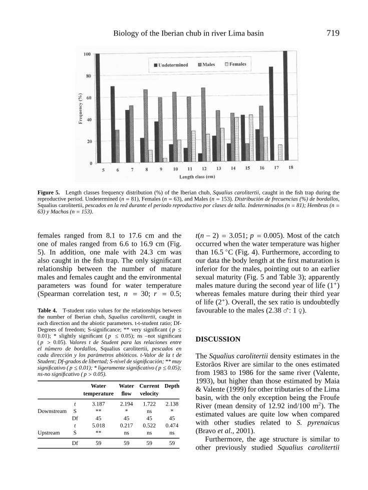
Biology of the Iberian chub in river Lima basin 719
Figure 5. Length classes frequency distribution (%) of the Iberian chub, Squalius carolitertii, caught in the fish trap during thereproductive period. Undetermined (n = 81), Females (n = 63), and Males (n = 153). Distribucion de frecuencias (%) de bordallos,Squalius carolitertii, pescados en la red durante el periodo reproductivo por clases de talla. Indeterminados (n = 81); Hembras (n =63) y Machos (n = 153).
females ranged from 8.1 to 17.6 cm and theone of males ranged from 6.6 to 16.9 cm (Fig.5). In addition, one male with 24.3 cm wasalso caught in the fish trap. The only significantrelationship between the number of maturemales and females caught and the environmentalparameters was found for water temperature(Spearman correlation test, n = 30; r = 0.5;
Table 4. T-student ratio values for the relationships betweenthe number of Iberian chub, Squalius carolitertii, caught ineach direction and the abiotic parameters. t-t-student ratio; Df-Degrees of freedom; S-significance; ** very significant ( p ≤0.01); * slightly significant ( p ≤ 0.05); ns –not significant( p > 0.05). Valores t de Student para las relaciones entreel numero de bordallos, Squalius carolitertii, pescados encada direccion y los parametros abioticos. t-Valor de la t deStudent; Df-grados de libertad; S-nivel de significacion; ** muysignificativo ( p ≤ 0.01); * ligeramente significativo ( p ≤ 0.05);ns-no significativo ( p > 0.05).
Water Water Current Depthtemperature flow velocity
t 3.187 2.194 1.722 2.138Downstream S ** * ns *
Df 45 45 45 45t 5.018 0.217 0.522 0.474
Upstream S ** ns ns ns
Df 59 59 59 59
t(n − 2) = 3.051; p = 0.005). Most of the catchoccurred when the water temperature was higherthan 16.5 ◦C (Fig. 4). Furthermore, according toour data the body length at the first maturation isinferior for the males, pointing out to an earliersexual maturity (Fig. 5 and Table 3); apparentlymales mature during the second year of life (1+)whereas females mature during their third yearof life (2+). Overall, the sex ratio is undoubtedlyfavourable to the males (2.38 ♂: 1 ♀).
DISCUSSION
The Squalius carolitertii density estimates in theEstoraos River are similar to the ones estimatedfrom 1983 to 1986 for the same river (Valente,1993), but higher than those estimated by Maia& Valente (1999) for other tributaries of the Limabasin, with the only exception being the FroufeRiver (mean density of 12.92 ind/100 m2). Theestimated values are quite low when comparedwith other studies related to S. pyrenaicus(Bravo et al., 2001).
Furthermore, the age structure is similar toother previously studied Squalius carolitertii

720 Maia et al.
populations in tributaries of the Lima River(Valente, 1993), and similar to the ones forother Iberian sister species such as S. pyrenaicus(Fernandez-Delgado & Herrera, 1995; Geraldes& Collares-Pereira, 1995; Lobon-Cervia &Sostoa, 1987 and Pires et al., 2000), althoughthese authors have referred to some populationswhere fish attained 6 to 7 years of age.
The results for the length-weight relationshipare in agreement with those referred to by Valente& Alexandrino (1987) and Valente (1993). Also,an increase of the condition factor in the springhas been referred to by Fernandez-Delgado &Herrera (1995) for S. pyrenaicus. These authorsstated that the somatic condition tended to behigher in females than in males, which contrastwith the significantly higher somatic conditionfor the males that our results have revealed.However, Fernandez-Delgado & Herrera (1995)used the dry weight of eviscerated fish for theircalculations of the somatic condition whereas, inthis study, we utilized fresh weight. Nevertheless,the differences observed could be related tothe final development of the gonads in thespring as observed by Soriguer et al. (2000)for S. pyrenaicus and the influence of thegonads’ weight in the determination of the Fultoncondition factor (Wootton, 1990). In addition,the sex-ratio referred to by Fernandez-Delgado& Herrera (1995) and Soriguer et al. (2000) forS. pyrenaicus (1 ♀: 1 ♂) reveals an equilibriumbetween sexes in contrast with the 2.38 ♂: ♀found in the Estoraos River for S. carolitertii.Such a sex ratio is difficult to explain, but thesexing procedure in our study did not involvevisual inspection of the gonads. However, and asstated by Soriguer et al. (2000) for S. pyrenaicus,the number of immature fish is very high even inupper size classes where mature fish are expectedand where the predominance of females iscommon in most cyprinids species (Mann, 1991).
The back-calculated lengths revealed valuessimilar to those referred to by Valente (1993) forIberian chub populations in other tributaries ofthe Lima River, except for the first year of growthwhere our results are higher. The estimated finallength value is superior to those referred to byValente (1990 and 1993) for tributaries of the
Lima and Douro basins, and even for the chubpopulation inhabiting the upper Estoraos Riverstretches. Mean length values at age are withinthe range observed in other Iberian populationsof S. pyrenaicus (Lobon-Cervia & Sostoa, 1987;Geraldes & Collares-Pereira, 1995; Fernandez-Delgado & Herrera, 1995 and Pires et al., 2000).Furthermore, the final length values referred toS. pyrenaicus (Lobon-Cervia & Sostoa, 1987and Fernandez-Delgado & Herrera, 1995) arecomparable to ours except in the case of theSorraia River population (Geraldes & Collares-Pereira, 1995). It appears that the population ofSqualius carolitertii in the Estoraos River couldreach a bigger theoretical maximum length thanthe Portuguese populations of S. pyrenaicus, eventhough its growth rate is smaller.
Sexual maturity was reached by the males at asmaller size (6.6 cm for the males and 8.1 cm forthe females). Similar results have been obtainedfor S. pyrenaicus (Fernandez-Delgado & Herrera,1995) and for S. torgalensis (Magalhaes etal., 2003). Mann (1991) also stated that inmost cyprinids females grow faster and becamesexually mature later than males. Fernandez-Delgado & Herrera (1995) and Geraldes &Collares-Pereira (1995) had already observedthat males matured at age 2+ and females at age3+ in S. pyrenaicus. Only Magalhaes et al. (2003)refer to the same age of maturation (2+) for bothsexes for S. torgalensis.
Our results also point out that water tempe-rature is apparently the major factor associatedwith the fish movements as also stated by Maia& Valente (2004) for Chondrostoma oligolepis.In addition, Santos et al (2002) found that riverflow was the only factor significantly correlatedto Iberian chub upstream daily movements in afish lift in the Lima River. This is in contrast withour results that revealed the influence of the riverflow only for the downstream movements. Santoset al. (2002) also stated that the Iberian chub ma-jor movements occurred from mid-April onwardswhen water temperature increases to values ran-ging from 12 to 14 ◦C which agrees with our re-sults. Baras & Cherry (1990) also found for thepopulation of Barbus barbus in the Ourthe Ri-ver, Belgium, that fish movements increased fo-

Biology of the Iberian chub in river Lima basin 721
llowing the rise of water temperature except fora few downstream movements caused by displa-cements due to high flow conditions. According-ly, Rodriguez-Ruiz & Granado-Lorencio (1992)found that water temperature is the major fac-tor controlling migration and the periodicity ofreproduction in three species of cyprinids in theGuadalete River (southwest of Spain). In conclu-sion, locomotion activity is enhanced by the va-riation of the environmental parameters, mainlythe rise of water temperature, and is associated tothe proximity of the reproductive period and thesearch for appropriated spawning grounds.
Overall, the results obtained in the presentstudy suggest that the characteristics of thispopulation do not differ substantially from thosefound for other Squalius carolitertii populationsas well as for its sister species, S. pyrenaicuspopulations, even though Squalius carolitertiicould reach a bigger theoretical maximum lengththan the Portuguese populations of S. pyrenaicus.Further research should then be directed tostudies on the inventory and characterizationof the spawning grounds in the Estoraos Riverand to the description of the Iberian chubspawning behaviour. Such information willcertainly improve the knowledge of this speciesand will also allow for the adjustment ofmanagement strategies.
ACKNOWLEDGMENTS
This research was partially funded by the Portu-guese Ministry of Science and Technology underthe projects PRAXIS XXI 3/3.2/BIA/41/94 andPRAXIS XXI/P/BIA/10245/1998. This studywas also partially funded by Ponte de LimaMunicipality under the project Inventory of thefish community in the Protected Area of the La-goons of Bertiandos and of Sao Pedro de Ar-cos. We thank the facilities granted by DireccaoGeral das Florestas. We are especially gratefulto Jorge Silva, Susana Carneiro, Pedro Correia,and Antonio Sa Pereira for their help during fieldwork. Last, thanks are due to the two anonymousreviewers whose contributions have greatly im-proved the final version of the manuscript.
REFERENCES
ALVES, M. J., M. J. COLLARES-PEREIRA, T. E.DOWLING & M. M. COELHO. 2002. Thegenetics of maintenance of an all-male lineage inthe Squalius alburnoides complex. J. Fish Biol.,60: 649-662.
BAGENAL, T. B. & F. W. TESCH. 1978. Age andGrowth. In: Methods for assessment of fishproduction in fresh waters. Bagenal, T. B. (Ed.):101-136. IPB Handbook, 3. 3rd Edition: BlackwellScientific Publications, Oxford-London.
BARAS, E. & B. CHERRY. 1990. Seasonal activitiesof female barbel Barbus barbus (L.) in the riverOurthe (Southern Belgium) as revealed by radio-tracking. Aquatic Living Resources, 3: 283-294.
BRAVO, R., M. C. SORIGUER, N. VILLAR &J. A. HERNANDO. 2001. The dynamics offish populations in the Palancar stream, a smalltributary of the river Guadalquivir, Spain. ActaOecologica, 22: 9-20.
BRITO, R. M., J. BRIOLAY, N. GALTIER, Y. BOU-VET & M.M. COELHO. 1997. Phylogenetic re-lationships within genus Leuciscus (Pisces: Cypri-nidae) in Portuguese freshwaters, based on mito-chondrial DNA cytochrome b sequences. Molecu-lar Phylogenetics and Evolution, 8: 435-442.
CARMONA, J. A. & I. DOADRIO. 2000. Threate-ned fishes of the world: Leuciscus carolitertii Doa-drio, 1988 (Cyprinidae). Environmental Biology ofFishes, 57: 96.
COELHO, M. M., R. M. BRITO, T. R. PACHECO,D. FIGUEIREDO & A. M. PIRES. 1995. Geneticvariation and divergence of Leuciscus pyrenaicusand L. carolitertii (Pisces: Cyprinidae). J. FishBiol., 47: 243-258.
DOADRIO, I. 1988. Leuciscus carolitertii n. sp. fromthe Iberian Peninsula. Senckenbergiana biologica,68: 301-309.
DOADRIO, I. (ed.) 2001. Atlas y libro rojo de lospeces continentales de Espana. Direccion Generalde Conservacion de la Naturaleza. Museo Nacionalde Ciencias Naturales, Madrid, 364 pp.
ECONOMIDIS, P. S. 2002. Biology of rare andendangered non-migratory fish species: problemsand constraints. In: Conservation of FreshwaterFishes: Options for the Future. Collares-Pereira,M. J.; Coelho, M. M. & Cowx, I. G. (eds): 81-89.Blackwell Science. Fishing News Book, Oxford,London.

722 Maia et al.
FERNANDEZ-DELGADO, C. & M. HERRERA.1995. Age structure, growth and reproduction ofLeuciscus pyrenaicus in an intermittent steam inthe Guadalquivir river basin, Southern Spain. J.Fish Biol., 46: 371-380.
FONTOURA, A. P. (1989). Evolucao da qualidadeda agua do rio Lima. Actas do Coloquio Luso-espanhol sobre Ecologia das Bacias Hidrograficase Recursos Zoologicos. March 23-25, 1988.Faculty of Sciences, Porto, Portugal: 149-154.
GERALDES, A. M. & M. J. COLLARES-PEREIRA.1995. Preliminary insight into age and growth ofthe Iberian chub (Leuciscus pyrenaicus) in theSorraia system. Folia Zoologica, 44: 159-165.
ICN. 2004. Livro vermelho dos vertebrados de Portugal–revisao. Classificacao-resultados preliminares.Peixes. [on-line]. Retrieved October 12, 2004 fromICN on the World Wide Web: http://www.icn.pt/documentos/livrovermelho/ClassifCritPeixes.pdf
LOBON-CERVIA, J. 1991. Dinamica de Poblacio-nes de Peces en Rios. Pesca electrica y metodosde capturas sucesivas en la estima de abundancias.Monografias del Museo Nacional de Ciencias Na-turales, 3: 1-156.
LOBON-CERVIA, J. & A. SOSTOA. 1987. El cre-cimiento del Cacho (Leuciscus cephalus pyraenai-cus Gunther, 1862) en el rıo Jarama (cuenca delTajo). Donana, Acta Vertebrata, 14: 41-51.
MAGALHAES, M. F., I. J. SCHLOSSER & M. J.COLLARES-PEREIRA. 2003. The role of life historyin the relationship between population dynamicsand environmental variability in two Mediterra-nean stream fishes. J. Fish Biol., 63: 300-317.
MAIA, C. F. Q. & A. C. N. VALENTE. 1999. Thebrown trout Salmo trutta L. populations in the riverLima catchment. Limnetica, 17: 119-126.
MAIA, H. & A. VALENTE. 2004. Biology of theroach (Chondrostoma macrolepidotus) populationin the Protected Area of the Lagoons of Bertiandosand of Sao Pedro de Arcos (Northern Portugal).Revista de Biologia (Lisboa), 22: 65-78.
MANN, R. H. K. 1991. Growth and Production. In:Cyprinid Fishes, Systematic, Biology and Exploi-tation. In: Winfield, I. J. & Nelson, J. S. (eds.).:456-482. Chapman & Hall, London.
OMBREDANE, D. & J. L. AGLINIERE, J. L.(1992). Les ecailles et leurs utilisations enEcologie halieutique. In : Tissus durs et age indi-viduel des vertebres. Bagliniere, J. L., Castanet, J.,Conand, F., Meunier, F. J. (eds.).: 151-192. Collo-
que national, Bondy, France, 4-6 of March 1991.Colloques et Seminaires ORSTOM-INRA.
PIRES A. M., I. G. COWX & M. M. COELHO.2000. Life history strategy of Leuciscus pyrenaicusin intermittent streams of the Guadiana basin.Cybium, 24: 287-297.
RODRIGUEZ-RUIZ, A. & C. GRANADO-LOREN-CIO. 1992. Spawning period and migration ofthree species of cyprinids in a stream withMediterranean regimen (SW Spain). J. Fish Biol.,41: 545-556.
SANJUR, O. I., J. A CARMONA & I. DOADRIO.2003. Evolutionary and geographical patterns wit-hin Iberian populations of the genus Squalius in-ferred from molecular data. Molecular Phylogene-tics and Evolution, 29: 20-30.
SANTOS, J. M., M. T. FERREIRA, F. N. GO-DINHO & J. BOCHECHAS. 2002. Performanceof fish lift recently builds at the Touvedo Dam onthe Lima River, Portugal. Journal of Applied Ich-thyology, 18: 118-123.
SANTOS, J. M., F. N. GODINHO & M. T. FE-RREIRA. 2004. Microhabitat use by Iberian naseChondrostoma polylepis and Iberian chub Squaliuscarolitertii in three small streams, north-west Por-tugal. Ecology of Freshwater Fish, 13: 223-230.
SNPRCN. 1991. Livro vermelho dos vertebrados dePortugal. Vol. II – Peixes dulciaquıcolas e mi-gradores. Servico Nacional de Parques, Reser-vas e Conservacao da Natureza, Lisbon: 55 pp.
SOKAL, R. R. & F. J. ROHLF. 1987. Introduction toBiostatistics. 2nd Edition. W. H. Freeman and Co.,San Francisco, 363 pp.
SORIGUER, M. C., R. BRAVO, C. VALLESPIN, C.GOMEZ-CAMA. & J. A. HERNANDO. 2000.Reproductive strategies of two species of cyprinidsin a stream with Mediterranean regimen (SWSpain). Arch. Hydrobiol., 148: 119-134.
VALENTE, A. C. N. 1990. As populacoes piscıcolasdo rio Febros. 1o Congresso Internacional sobre orio Douro. Observatorio, 1: 421-437.
VALENTE, A. C. N. 1993. Biologia e dinamica daspopulacoes de truta-de-rio, Salmo trutta L., dabacia hidrografica do rio Lima. Ph.D Thesis,Universidade do Porto. 244 pp.
VALENTE, A. C. N. & P. J. ALEXANDRINO.1987. La ictiofauna del embalse de Bemposta (rıoDuero, Portugal). Actas IV Congreso Espanol deLimnologıa, Sevilla, Espana: 353-358.
WOOTTON, R. J. 1990. Ecology of Teleost Fishes.Chapman & Hall. London, 386 pp.

Limnetica, 25 (3-4): xx-xx (2006)Limnetica, 25 (3): 723-732 (2006)c© Asociacion Espanola de Limnologıa, Madrid. Spain. ISSN: 0213-8409
Usos del suelo en las cuencas hidrograficas de los humedales del AltoGuadalquivir: Importancia de una adecuada gestion
Fernando Ortega, Gema Parra y Francisco Guerrero∗
Departamento de Biologıa Animal, Biologıa Vegetal y Ecologıa. Facultad de Ciencias Experimentales. Universi-dad de Jaen. Campus de Las Lagunillas s/n. E-23071 Jaen.3Hola∗ Corresponding author: [email protected]
RESUMEN
Usos del suelo en las cuencas hidrograficas de los humedales del Alto Guadalquivir: Importancia de una adecuadagestion
Se ha realizado la delimitacion y valoracion de los usos del suelo en la cuenca hidrografica de 22 humedales de la comarcadel Alto Guadalquivir. Para dicha valoracion se ha diferenciado entre cultivos (herbaceos y arboreos); vegetacion natural(monte bajo), terrenos forestales, pastizales, humedales desecados y terrenos urbanizados. El olivar es la actividad que mayorocupacion de suelo presenta en el territorio estudiado. Las actividades regularmente desarrolladas en el cultivo intensivodel olivar provocan el incremento de perturbaciones que repercuten sobre toda la cuenca de drenaje y particularmente en lacalidad de las aguas y la conservacion del humedal. Los resultados obtenidos se discuten en el contexto de la conservacion delos humedales de la comarca del Alto Guadalquivir.
Palabras clave: Humedales, Paisajes mediterraneos, Cuencas de drenaje, Usos del suelo, Olivar.
ABSTRACT
Land uses in the hydrographic basins of the Alto Guadalquivir wetlands: The importance of a suitable management
Drainage basin demarcation and the land uses identification have been carried out in 22 wetlands from the Alto Guadalquivirarea. The land uses identified were crops (herbaceous and tree crops); natural vegetation; forests; grazing land; desiccatedwetland and urban areas. Olive tree growing was the predominant soil use detected. The regular activities carried out inthe olive intensive agriculture generate increased perturbations over the whole drainage basin and especially on the waterquality and wetland conservation. The results obtained are discussed within the context of the Alto Guadalquivir wetlandconservation.
Keywords: Wetlands, Mediterranean landscapes, Catchment areas, Land uses, Olive tree crops.
INTRODUCCION
Los humedales se encuentran entre los espa-cios naturales con mayor valor ambiental, tantopor el mantenimiento de una elevada diversidadbiologica, lo que establece claramente su relevan-cia ecologica; como por la importancia que hantenido para el desarrollo de la humanidad, des-de una perspectiva cultural e historica, economi-ca, como fuente de riqueza sostenible, y cientıfica(Bernaldez, 1987; Williams, 1999).
El estudio de los humedales ha permitidoen los ultimos anos poner de manifiesto larelevancia que las cuencas hidrograficas tienensobre el funcionamiento de estos ecosistemasacuaticos (vease por ejemplo Gibson et al.,1995; Ulrich, 1997; Morales-Baquero et al.,1999; Morales-Baquero & Conde-Porcuna,2000; Maler, 2000; Matias, 2001; Istvanovics& Somlyody, 2001), siendo por ello actual-mente consideradas como los instrumentosmas adecuados en la gestion de los humedales

724 Ortega et al.
y en la conservacion de su integridad ecologicaoriginal (INIMA, 1996; Ors, 1999).
Una buena gestion de las cuencas de drenajees, por tanto, fundamental para mantener la ca-lidad ecologica de estos ecosistemas, ya que loshumedales dependen directamente de los proce-sos hidrogeomorfologicos, biologicos y humanos(agricultura, deforestacion, regulacion, urbaniza-cion, etcetera) que se producen en los ecosiste-mas terrestres que drenan hacia sus cubetas. Portodo ello, resultarıa imposible comprender com-pletamente el estado actual de un humedal sintener presentes los usos del suelo y los cambiosproducidos en su cuenca hidrografica.
Esta valoracion sobre la importancia de unacorrecta gestion de las cuencas de drenaje en laconservacion de los humedales ha quedado reco-gida en diversos planes y convenios, tanto en elambito internacional (convenio de Ramsar y con-venio sobre la Biodiversidad Biologica), comonacional (Plan Estrategico Espanol para la Con-servacion y el Uso Racional de los Humedales) yregional (Plan Andaluz de Humedales).
Andalucıa posee un conjunto de humedalesmuy destacable a nivel de la Penınsula Iberica,con la presencia de una gran variedad de tiposecologicos, algunos de los cuales son unicosen el contexto de la Union Europea (Molina etal., 2002). Dentro de esta comunidad autonoma,la comarca del Alto Guadalquivir presenta unode los conjuntos palustres menos conocidos yestudiados, con una amplia variedad de tamanosy tipologıas presentes (Ortega et al., 2003).
Este desconocimiento ha llevado a que solo tresde ellos hayan sido incluidos hasta el momentodentro de la red de espacios protegidos de An-dalucıa. Sin embargo, estudios recientes (Ortegaet al., 2004) han puesto de manifiesto la existen-cia de un conjunto de humedales, agrupados bajola denominacion de red palustre “lagunas del Al-to Guadalquivir”, que por sus valores naturalesestan en vıas de ser incluidos dentro el InventarioAndaluz de Humedales y en las propuestas anda-luzas para formar parte de la Red Natura 2000.
De este modo, este estudio se plantea comoobjetivo primordial la delimitacion y la descrip-cion de los usos del suelo en las cuencas de dre-naje de los humedales incluidos en la red palus-
tre “lagunas del Alto Guadalquivir”. Este obje-tivo es fundamental para el conocimiento y fun-cionamiento de estos humedales, proporcionan-do de este modo una herramienta basica parala correcta gestion y conservacion de las zonashumedas. Los resultados de este estudio podranservir de base comparativa para evaluar futurosprocesos de cambios en los usos del suelo ysu consiguiente repercusion sobre los humedalesdel Alto Guadalquivir.
AREA DE ESTUDIO
La comarca del Alto Guadalquivir se localiza alNordeste de Andalucıa (Espana), englobando lacasi totalidad de la provincia de Jaen y la partemas oriental de la provincia de Cordoba.
Uno de los elementos caracterısticos de estacomarca es la presencia del valle del rıo Guadal-quivir y la gran actividad de tipo agrıcola desarro-llada en el mismo, hecho que ha conducido a ladegeneracion de sus ecosistemas naturales en ge-neral y de los humedales en particular (Guerreroet al., 2002 y 2005).
La mayorıa de estos son lagunas estacionalesde variado tamano y origen geologico, habiendosido inventariadas hasta la actualidad un total de 90humedales (Ortega et al., 2003). De este colectivose ha seleccionado para este estudio 22 hume-dales (Fig. 1; Tabla 1) englobados bajo la red palus-tre ‘‘lagunas del Alto Guadalquivir’’ (Ortega et al.,2004) en funcion de su estado de conservacion yde la valoracion de sus comunidades acuaticas.
MATERIAL Y METODOS
Para la descripcion y estudio pormenorizado delos usos del suelo llevada a cabo en las cuen-cas de drenaje de los humedales incluidos en es-te estudio, se han utilizado ortofotografıas digita-les a color a escala 1:10.000 (Junta de Andalucıa,2003); cartografıa a escalas 1:50.000 y 1:10.000,para la correcta delimitacion de las cuencas ver-tientes, ası como diversas jornadas de campo ne-cesarias para cumplimentar a detalle los aspectosque no han podido ser realizados en gabinete.

Usos del suelo en cuencas de los humedales del Alto Guadalquivir 725
Figura 1. Comarca del Alto Guadalquivir y localizacion de los humedales incluidos en este estudio. 1: Laguna Honda; 2: Lagunadel Chinche; 3: Laguna de la Quinta; 4: Laguna del Rincon del Muerto; 5: Laguna de Hituelo; 6: Laguna de Naranjeros; 7: Lagunade las Ceras; 8: Laguna del Ranal; 9: Laguna de Casillas; 10: Laguna de las Navas; 11: Laguna de Villardompardo; 12: Lagunade Garcıez; 13: Laguna de Prados del Moral; 14: Laguna de Brujuelo; 15: Laguna Grande; 16: Laguna Chica; 17: Laguna deArgamasilla; 18: Laguna de Santisteban; 19: Laguna de Perales; 20: Laguna de Pedernoso; 21: Laguna de Siles; 22: Laguna deOrcera. Alto Guadalquivir region and location of the wetlands included in this study. 1: Laguna Honda; 2: Laguna del Chinche; 3:Laguna de la Quinta; 4: Laguna del Rincon del Muerto; 5: Laguna de Hituelo; 6: Laguna de Naranjeros; 7: Laguna de las Ceras;8: Laguna del Ranal; 9: Laguna de Casillas; 10: Laguna de las Navas; 11: Laguna de Villardompardo; 12: Laguna de Garcıez; 13:Laguna de Prados del Moral; 14: Laguna de Brujuelo; 15: Laguna Grande; 16: Laguna Chica; 17: Laguna de Argamasilla; 18:Laguna de Santisteban; 19: Laguna de Perales; 20: Laguna de Pedernoso; 21: Laguna de Siles; 22: Laguna de Orcera.
Con todo ello se ha procedido a una delimitacionde la cuenca hidrografica superficial de cada hu-medal, tras lo cual se ha acometido la identifi-cacion y cuantificacion en terminos de superfi-cie ocupada (programas Mulhacen y ArcView),de cada uno de los usos del suelo.
Se ha diferenciado entre cultivos (herbaceos yarboreos); vegetacion natural (monte bajo), terre-nos forestales, pastizales, humedales desecados yterrenos urbanizados (normalmente como corti-jos aislados). Dentro de los cultivos se ha dife-renciado entre la presencia de cultivos de regadıoo de secano. Igualmente, dentro de los cultivosarboreos (entre 100-125 arboles por hectarea), seha hecho hincapie en la distincion de la edad delas plantaciones, considerando olivares madurosa aquellos que presentan una edad superior a 10anos. Finalmente destacar la localizacion y car-tografiado de antiguas zonas humedas, incluidasen las cuencas de algunos de los humedales ob-
jeto de estudio, que actualmente se encuentrandesecadas por accion antropica, y que constitu-yen areas de gran importancia que pueden supo-ner zonas potenciales para la aplicacion de un fu-turo plan de restauracion ecologica.
RESULTADOS
En la Tabla 1 se presentan algunas caracterısticaslimnologicas de los humedales estudiados. Comopuede observarse, estos humedales se situan entrelos 265 y los 1280 metros de altitud, habiendosido clasificados en dos tipologıas (Ortega et al.,2003), humedales asociados a zonas de montana(lagunas de Siles y Orcera) y asociados al valledel rıo Guadalquivir (el resto). La mayor partede ellos presentan, por su ubicacion geografica,un regimen hıdrico (segun Cirujano, 1995), quelas situa como lagunas o humedales estacionales
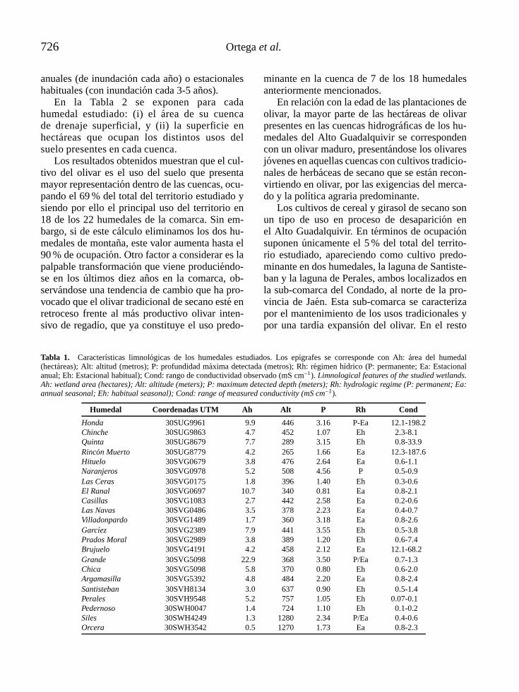
726 Ortega et al.
anuales (de inundacion cada ano) o estacionaleshabituales (con inundacion cada 3-5 anos).
En la Tabla 2 se exponen para cadahumedal estudiado: (i) el area de su cuencade drenaje superficial, y (ii) la superficie enhectareas que ocupan los distintos usos delsuelo presentes en cada cuenca.
Los resultados obtenidos muestran que el cul-tivo del olivar es el uso del suelo que presentamayor representacion dentro de las cuencas, ocu-pando el 69 % del total del territorio estudiado ysiendo por ello el principal uso del territorio en18 de los 22 humedales de la comarca. Sin em-bargo, si de este calculo eliminamos los dos hu-medales de montana, este valor aumenta hasta el90 % de ocupacion. Otro factor a considerar es lapalpable transformacion que viene produciendo-se en los ultimos diez anos en la comarca, ob-servandose una tendencia de cambio que ha pro-vocado que el olivar tradicional de secano este enretroceso frente al mas productivo olivar inten-sivo de regadıo, que ya constituye el uso predo-
minante en la cuenca de 7 de los 18 humedalesanteriormente mencionados.
En relacion con la edad de las plantaciones deolivar, la mayor parte de las hectareas de olivarpresentes en las cuencas hidrograficas de los hu-medales del Alto Guadalquivir se correspondencon un olivar maduro, presentandose los olivaresjovenes en aquellas cuencas con cultivos tradicio-nales de herbaceas de secano que se estan recon-virtiendo en olivar, por las exigencias del merca-do y la polıtica agraria predominante.
Los cultivos de cereal y girasol de secano sonun tipo de uso en proceso de desaparicion enel Alto Guadalquivir. En terminos de ocupacionsuponen unicamente el 5 % del total del territo-rio estudiado, apareciendo como cultivo predo-minante en dos humedales, la laguna de Santiste-ban y la laguna de Perales, ambos localizados enla sub-comarca del Condado, al norte de la pro-vincia de Jaen. Esta sub-comarca se caracterizapor el mantenimiento de los usos tradicionales ypor una tardıa expansion del olivar. En el resto
Tabla 1. Caracterısticas limnologicas de los humedales estudiados. Los epıgrafes se corresponde con Ah: area del humedal(hectareas); Alt: altitud (metros); P: profundidad maxima detectada (metros); Rh: regimen hıdrico (P: permanente; Ea: Estacionalanual; Eh: Estacional habitual); Cond: rango de conductividad observado (mS cm−1). Limnological features of the studied wetlands.Ah: wetland area (hectares); Alt: altitude (meters); P: maximum detected depth (meters); Rh: hydrologic regime (P: permanent; Ea:annual seasonal; Eh: habitual seasonal); Cond: range of measured conductivity (mS cm−1).
Humedal Coordenadas UTM Ah Alt P Rh Cond
Honda 30SUG9961 9.9 0446 3.16 P-Ea 12.1-198.2Chinche 30SUG9863 4.7 0452 1.07 Eh 12.3-8.111Quinta 30SUG8679 7.7 0289 3.15 Eh 10.8-33.91Rincon Muerto 30SUG8779 4.2 0265 1.66 Ea 12.3-187.6Hituelo 30SVG0679 3.8 0476 2.64 Ea 10.6-1.111Naranjeros 30SVG0978 5.2 0508 4.56 P 10.5-0.911Las Ceras 30SVG0175 1.8 0396 1.40 Eh 10.3-0.611El Ranal 30SVG0697 10.7 0340 0.81 Ea 10.8-2.111Casillas 30SVG1083 2.7 0442 2.58 Ea 10.2-0.611Las Navas 30SVG0486 3.5 0378 2.23 Ea 10.4-0.711Villadonpardo 30SVG1489 1.7 0360 3.18 Ea 10.8-2.611Garcıez 30SVG2389 7.9 0441 3.55 Eh 10.5-3.811Prados Moral 30SVG2989 3.8 0389 1.20 Eh 10.6-7.411Brujuelo 30SVG4191 4.2 0458 2.12 Ea 12.1-68.21Grande 30SVG5098 22.9 0368 3.50 P/Ea 10.7-1.311Chica 30SVG5098 5.8 0370 0.80 Eh 10.6-2.011Argamasilla 30SVG5392 4.8 0484 2.20 Ea 10.8-2.411Santisteban 30SVH8134 3.0 0637 0.90 Eh 10.5-1.411Perales 30SVH9548 5.2 0757 1.05 Eh 0.07-0.111Pedernoso 30SWH0047 1.4 0724 1.10 Eh 10.1-0.211Siles 30SWH4249 1.3 1280 2.34 P/Ea 10.4-0.611Orcera 30SWH3542 0.5 1270 1.73 Ea 10.8-2.311
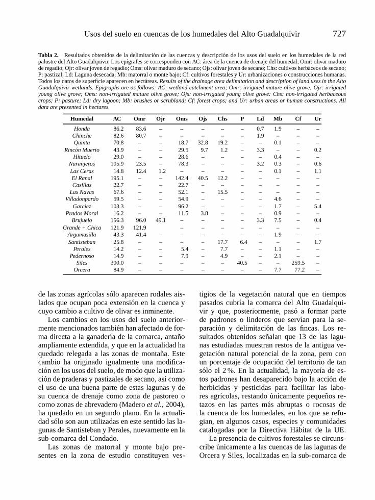
Usos del suelo en cuencas de los humedales del Alto Guadalquivir 727
Tabla 2. Resultados obtenidos de la delimitacion de las cuencas y descripcion de los usos del suelo en los humedales de la redpalustre del Alto Guadalquivir. Los epıgrafes se corresponden con AC: area de la cuenca de drenaje del humedal; Omr: olivar madurode regadıo; Ojr: olivar joven de regadıo; Oms: olivar maduro de secano; Ojs: olivar joven de secano; Chs: cultivos herbaceos de secano;P: pastizal; Ld: Laguna desecada; Mb: matorral o monte bajo; Cf: cultivos forestales y Ur: urbanizaciones o construcciones humanas.Todos los datos de superficie aparecen en hectareas. Results of the drainage area delimitation and description of land uses in the AltoGuadalquivir wetlands. Epigraphs are as follows: AC: wetland catchment area; Omr: irrigated mature olive grove; Ojr: irrigatedyoung olive grove; Oms: non-irrigated mature olive grove; Ojs: non-irrigated young olive grove: Chs: non-irrigated herbaceouscrops; P: pasture; Ld: dry lagoon; Mb: brushes or scrubland; Cf: forest crops; and Ur: urban areas or human constructions. Alldata are presented in hectares.
Humedal AC Omr Ojr Oms Ojs Chs P Ld Mb Cf Ur
Honda 086.2 083.6 – – – – – 0.7 1.9 – –Chinche 082.6 080.7 – – – – – 1.9 – – –Quinta 070.8 – – 018.7 32.8 19.2 – – 0.1 – –
Rincon Muerto 043.9 – – 029.5 09.7 01.2 – 3.3 – – 0.2Hituelo 029.0 – – 028.6 – – – – 0.4 – –
Naranjeros 105.9 023.5 – 078.3 – – – 3.2 0.3 – 0.6Las Ceras 014.8 012.4 01.2 – – – – – 0.1 – 1.1El Ranal 195.1 – – 142.4 40.5 12.2 – – – – –Casillas 022.7 – – 022.7 – – – – – – –
Las Navas 067.6 – – 052.1 – 15.5 – – – – –Villadonpardo 059.5 – – 054.9 – – – – 4.6 – –
Garciez 103.3 – – 096.2 – – – – 1.7 – 5.4Prados Moral 016.2 – – 011.5 03.8 – – – 0.9 – –
Brujuelo 156.3 096.0 49.1 – – – – 3.3 7.5 – 0.4Grande + Chica 121.9 121.9 – – – – – – – –
Argamasilla 043.3 041.4 – – – – – – 1.9 – –Santisteban 025.8 – – – – 17.7 06.4 – – – 1.7
Perales 014.2 – – 005.4 – 07.7 – – 1.1 – –Pedernoso 014.9 – – 007.9 – 04.9 – – 2.1 – –
Siles 300.0 – – – – – 40.5 – – 259.5 –Orcera 084.9 – – – – – – – 7.7 077.2 –
de las zonas agrıcolas solo aparecen rodales ais-lados que ocupan poca extension en la cuenca ycuyo cambio a cultivo de olivar es inminente.
Los cambios en los usos del suelo anterior-mente mencionados tambien han afectado de for-ma directa a la ganaderıa de la comarca, antanoampliamente extendida, y que en la actualidad haquedado relegada a las zonas de montana. Estecambio ha originado igualmente una modifica-cion en los usos del suelo, de modo que la utiliza-cion de praderas y pastizales de secano, ası comoel uso de una buena parte de estas lagunas y desu cuenca de drenaje como zona de pastoreo ocomo zonas de abrevadero (Madero et al., 2004),ha quedado en un segundo plano. En la actuali-dad solo son aun utilizadas en este sentido las la-gunas de Santisteban y Perales, nuevamente en lasub-comarca del Condado.
Las zonas de matorral y monte bajo pre-sentes en la zona de estudio constituyen ves-
tigios de la vegetacion natural que en tiempospasados cubrıa la comarca del Alto Guadalqui-vir y que, posteriormente, paso a formar partede padrones o linderos que servıan para la se-paracion y delimitacion de las fincas. Los re-sultados obtenidos senalan que 13 de las lagu-nas estudiadas muestran restos de la antigua ve-getacion natural potencial de la zona, pero conun porcentaje de ocupacion del territorio de tansolo el 2 %. En la actualidad, la mayorıa de es-tos padrones han desaparecido bajo la accion deherbicidas y pesticidas para facilitar las labo-res agrıcolas, restando unicamente pequenos re-tazos en las partes mas abruptas o rocosas dela cuenca de los humedales, en los que se refu-gian, en algunos casos, especies y comunidadescatalogadas por la Directiva Habitat de la UE.
La presencia de cultivos forestales se circuns-cribe unicamente a las cuencas de las lagunas deOrcera y Siles, localizadas en la sub-comarca de

728 Ortega et al.
Tabla 3. Humedales desecados que se integran dentro de alguna de las cuencas de drenaje incluidas en el presente estudio. Drywetlands located in some of the drainage areas included in the present study.
Humedal Cuenca Area (ha) Estado actual Uso actual
Laguna de Casasola Rincon Muerto 2.5 Colmatada, cultivada GirasolLaguna Honda Honda 1.1 Drenada, colmatada Pastizal
Laguna del Chinche II Chinche 2.1 Drenada, colmatada PastizalLaguna de Rumpisaco Naranjeros 1.6 Drenada, colmatada Pastizal
Laguna de Ciruena Brujuelo 2.8 Drenada, colmatada Carrizal
la Sierra de Segura, al lımite con la provincia deAlbacete. En ella se llevaron a cabo antiguas re-poblaciones de pinares (Pinus nigra y Pinus pi-naster) para la explotacion de resina y madera delos montes de dominio publico. En ambos casosse trata de pinares maduros que ocupan la mayorparte del territorio junto a zonas de pastizal y re-tazos de encinar o matorral.
Incluidos en las cuencas de algunos de los hu-medales objeto de estudio, aparecen cubetas ad-yacentes de distinto tamano, que se encuentran enla actualidad desecadas y colmatadas por la ac-cion agrıcola, ası como drenadas hacia la cubetaprincipal (Tabla 3). Estos humedales se compor-tan en la actualidad como ocasionales, acumulan-do agua durante poco tiempo solo en anos lluvio-sos y drenando la sobrante al humedal principal.
Finalmente indicar que en la periferia delas lagunas aparecen diversos tipos de cons-trucciones humanas, que van desde pueblos oaldeas como Santisteban del Puerto y Garcıez,a zonas de urbanizaciones recreativas, alma-zaras y cortijos, como sucede por ejemplo,en las cuencas de las lagunas de Naranjeros,Rincon del Muerto, Las Ceras y Brujuelo. Lainfluencia de estas construcciones es diversay en general constituyen un impacto negativo,ya sea por las actividades de desecacion omodificacion realizadas en la vecina lagunapara su uso agrıcola, ganadero, recreativo,etcetera. Igualmente, los recientes cambiosagrıcolas de la comarca han fomentado en losultimos anos la transformacion de las cubetaslacustres en balsas de riego para el olivar(Ortega et al., 2005), ası como en balsasde alpechın de las almazaras, actividad estaultima, que afecta a varios humedales en lacomarca (lagunas de Garcıez y del Ranal).
DISCUSION
La region mediterranea ha sufrido desde tiem-pos remotos fuertes transformaciones a conse-cuencia de la actividad humana, siendo las acti-vidades pastoril y agrıcola las que mayores re-percusiones han tenido en los cambios del pai-saje registrados en esta region. La comarca delAlto Guadalquivir muestra una problematica am-biental que se manifiesta claramente asociada aun proceso de intensificacion agrıcola (Guerre-ro et al., 2005). Los resultados obtenidos mues-tran la dominancia del olivar sobre el resto decultivos y usos del suelo; quedando igualmen-te patente la progresiva transformacion del oli-var tradicional de secano en un olivar intensi-vo de regadıo (Moraga, 2002), proceso que seesta llevando a cabo no solo en el Alto Guadal-quivir, sino tambien en el resto de Andalucıa.
El cultivo del olivo estructura la economıade la mayorıa de los pueblos de esta comarca,actuando como catalizador cultural de la mul-titud de procesos economicos, sociales y cul-turales de esta sociedad (Anta, 2002; Palacios,2002). Sin embargo, desde un punto de vis-ta ambiental y de conservacion de la natura-leza, la implantacion de cualquier monoculti-vo o sistema de sobreexplotacion y la profun-da transformacion sufrida por ello en el terri-torio, genera fuertes transformaciones tanto enlos agrosistemas tradicionales como en los eco-sistemas adyacentes (Boutin & Jobin, 1998).
En este sentido hay que senalar que el olivares uno de los cultivos en los que las perdidas desuelo son mas elevadas, muy superiores a las ob-servadas en cultivos de cereal, girasol o en zonasde pastizal y matorral, con estimaciones en losolivares andaluces de una perdida media de 80

Usos del suelo en cuencas de los humedales del Alto Guadalquivir 729
toneladas de suelo por hectarea y ano, perdidasque se incrementan en territorios con fuerte pen-diente (Pastor et al., 1996). Si tenemos en cuentaque la tasa media de formacion de suelo en condi-ciones favorables es de una tonelada de suelo porhectarea y ano (Porta et al., 1994), podemos teneruna clara constatacion de uno de los principalesproblemas ambientales del territorio estudiado.
Del mismo modo, las actividades generadasen los agrosistemas se basan fundamentalmenteen la consecucion de resultados de cosecha, loque lleva asociado un incremento de aportes enforma de energıa auxiliar o productos agroquımi-cos. Este hecho se refleja de dos maneras bien di-ferentes en los ecosistemas acuaticos. En primerlugar a traves de una excesiva utilizacion de losrecursos hıdricos, tanto superficiales como sub-terraneos, con el incremento de pozos de extrac-cion, construccion de balsas de regadıo, deseca-cion de humedales, etcetera (Ortega et al., 2003;2005), efectos que van asociados al incrementode cultivos en regadıo y que va a tener especial re-
percusion en los humedales y en su balance hıdri-co anual. En segundo lugar, estas actividades semanifiestan en los efectos de los productos agro-quımicos sobre estos ecosistemas acuaticos.
Para reflejar este hecho, y aunque la esti-macion de las fuentes de nutrientes aloctonasa los sistemas acuaticos es de difıcil obten-cion (vease por ejemplo Irvine et al., 2000), seha realizado una valoracion de los aportes denitrogeno y fosforo total utilizando los coeficien-tes de exportacion de nutrientes aportados porJohnes et al. (1996). Estos coeficientes han si-do aplicados a los valores de superficie de uti-lizacion del suelo (actividad agrıcola, uso fo-restal y uso pascıcola), sin haber consideradootras actividades como por ejemplo la ganaderıao los aportes procedentes de la presencia hu-mana. Es importante hacer constar los elevadosvalores de aportacion de ambos nutrientes quese han obtenido (Tabla 4). Aunque estos coe-ficientes no han sido obtenidos especıficamen-te para la region Mediterranea, creemos que de
Tabla 4. Valores estimados mınimos y maximos de aportacion de nutrientes (nitrogeno y fosforo total) en los humedales delAlto Guadalquivir, en funcion de los usos del territorio. Los calculos se han realizado utilizando los coeficientes de exportacionde nutrientes de Johnes et al. (1996). Minimum and maximum estimated values of the external nutrient loads (total nitrogen andtotal phosphorus) in the Alto Guadalquivir wetlands as a function of the land use. Calculations were based on the nutrient exportcoefficients described by Johnes et al. (1996).
Humedal Agricultura Pasto Uso Forestal
Kg. N total Kg. P total Kg. N total Kg. P total Kg. N total Kg. P total
Honda 234.08 0 6061.00 056.848 0482.372 01.687 006.44 0.07 0.49 001.14 0.019 0.114Chinche 225.96 0 5850.75 054.876 0465.639 04.579 017.48 0.19 1.33 – – –Quinta 197.96 0 5125.75 048.076 0407.939 – – – – 000.06 0.001 0.006
Rincon Muerto 113.12 0 2929.00 027.472 0233.108 07.953 030.36 0.33 2.31 – – –Hituelo 080.08 0 2073.50 019.448 0165.022 – – – – 000.24 0.004 0.024
Naranjeros 285.04 0 7380.50 069.224 0587.386 07.712 029.44 0.32 2.24 000.18 0.003 0.018Las Ceras 038.08 00 986.00 009.248 0078.472 – – – – 000.06 0.001 0.006El Ranal 546.28 14 144.75 132.668 1125.727 – – – – – – –Casillas 063.56 0 1645.75 015.436 0130.979 – – – – – – –
Las Navas 189.28 0 4901.00 045.968 0390.052 – – – – – – –Villadonpardo 153.72 0 3980.25 037.332 0316.773 – – – – 002.76 0.046 0.276
Garciez 269.36 0 6974.50 065.416 0555.074 04.097 015.64 0.17 1.19 – – –Prados Moral 042.84 0 1109.25 010.404 0088.281 – – – – 000.54 0.009 0.054
Brujuelo 406.28 10 519.75 098.668 0837.227 07.953 030.36 0.33 2.31 004.50 0.075 0.45Grande + Chica 341.32 0 8837.75 082.892 0703.363 – – – – – – –
Argamasilla 115.92 0 3001.50 028.152 0238.878 – – – – 001.14 0.019 0.114Santisteban 049.56 0 1283.25 012.036 0102.129 15.424 058.88 0.64 4.48 – – –
Perales 036.68 00 949.75 008.908 0075.587 – – – – 000.66 0.011 0.066Pedernoso 035.84 00 928.00 008.704 0073.856 – – – – 001.26 0.021 0.126
Siles – – – – 97.605 372.60 4.05 28.35 155.70 2.595 15.57Orcera – – – – – – – – 050.94 0.849 5.094

730 Ortega et al.
modo cualitativo pueden constituir unas estimasde las tendencias de exportacion de nutrienteshacia los ecosistemas acuaticos, observandosecomo estas son siempre mayores para el casode la agricultura frente a las otras actividades.
El efecto directo mas inmediato asociado aeste aporte de nutrientes es la eutrofizacion delos sistemas acuaticos, con repercusiones sobrela estructura, funcionamiento y diversidad de losecosistemas. Esta contaminacion difusa es carac-terıstica de interacciones asimetricas como lasque se establecen entre un ecosistema que secomporta como donante (cuenca de drenaje delhumedal y donde se realizan los vertidos de pro-ductos agroquımicos) y un ecosistema receptor(sistema acuatico per se). Por todo ello, el tamanoy las caracterısticas de utilizacion de los usos delsuelo en las cuencas de drenaje de las lagunas sondeterminantes sobre la calidad del agua y el esta-do actual de los humedales, poniendose de mani-fiesto la importancia de un adecuado manejo de launidad cuenca-humedal (incluyendo a las cuen-cas hidrologicas superficial y subterranea de ali-mentacion) si se pretende conseguir una correctagestion y conservacion del patrimonio natural yla diversidad de los humedales.
En este sentido debemos indicar que resul-tados obtenidos en algunos de los ecosistemasaquı estudiados, como la laguna Honda (Cas-tro, 2004) o las lagunas de la Quinta, Grande yChica (Conde-Porcuna, com. per.), muestran unnivel de eutrofizacion que las situa en el ran-go de mesotroficas a hipertroficas. Igualmente,otras evidencias indirectas como la observacionde un crecimiento excesivo de algas epifıticas so-bre las praderas de macrofitos sumergidos (Be-cares et al., 2004); la desaparicion de la vege-tacion sumergida (Van den Berg et al., 1999) yel aumento de la turbidez asociado a un incre-mento del fitoplancton o a la resuspension de se-dimentos ante la ausencia de vegetacion acuati-ca (Weisner et al., 1997), hechos que tambienhan sido observadas en este conjunto de humeda-les, hacen denotar igualmente un elevado nivel deeutrofizacion de los mismos.
Por todo ello, si consideramos que para el ca-so de los humedales, la unidad funcional englobala cuenca de drenaje, surge la necesidad de pa-
sar de una gestion pasiva, como se ha ido practi-cando en la mayorıa de los casos, a una gestionactiva. Esta modalidad de gestion de los ecosiste-mas es mas adecuada para los espacios naturalesmediterraneos, en los que es necesario conside-rar tanto los valores naturales y culturales comola interaccion entre ambos (Garcıa-Mora & Mon-tes, 2003). De este modo, los criterios ambien-tales de usos del territorio, bastante introducidosen relacion con el urbanismo o la actividad in-dustrial, deberıan ganar peso progresivamente enrelacion con la actividad agrıcola, de modo queestas intervenciones permitan mantener determi-nados cuadros de integridad ecologica.
La adopcion de estas medidas de usos delterritorio en relacion con la actividad agrıco-la (Castle et al., 1999; Carreira & Garcıa-Ruiz,2005; Guerrero et al., 2005) o la aplicacion demodelos eco-economicos para el analisis de laspolıticas agro-ambientales (Oglethorpe & San-derson, 1999) permitirıa en un futuro mejorar lacalidad de nuestros humedales.
BIBLIOGRAFIA
ANTA, J. L. 2002. Parentesco y economıa en unasociedad giennense En: La cultura del aceite enAndalucıa. La tradicion frente a la modernidad.J.L. Anta y J. Palacios (eds.): 161-170. FundacionMachado. Sevilla, Espana.
BECARES, E., A. CONTY, C, RODRIGUEZ & S.BLANCO. 2004. Funcionamiento de los lagos so-meros mediterraneos. Ecosistemas, 2004/2 (URL:http://www.aeet.org/ecosistemas/042/revision3.htm).
BERNALDEZ, F. G. 1987. Las zonas encharcablesespanolas: el marco conceptual. En: Bases cientıfi-cas para la proteccion de los humedales en Es-pana. Real Academia de Ciencias Exactas, Fısicasy Naturales (ed.): 9-30. Madrid, Espana.
BOUTIN, C. & B. JOBIN. 1998. Intensity of agri-cultural practices and effects on adjacent habitats.Ecological Applications, 8: 544-557.
CARREIRA, J. & R. GARCIA-RUIZ. 2005. Princi-pios ecologicos para la sostenibilidad de agroeco-sistemas y del olivar en particular: presentacion deun marco conceptual general. En: La cultura delolivo: ecologıa, economıa, sociedad. J. L. Anta, J.Palacios y F. Guerrero (eds.): 333-366. Universi-dad de Jaen, Jaen, Espana.

Usos del suelo en cuencas de los humedales del Alto Guadalquivir 731
CASTLE, K., C. FROST & D. F. FLINT. 1999. TheLoch Leven project – buffer strips in practice ona catchment scale. Aspects of Applied Biology, 54:71-78.
CASTRO, M. C. 2004. Caracterizacion limnologicay variabilidad temporal de la comunidad planctoni-ca en laguna Honda (Jaen). Tesis Doctoral. Univer-sidad de Jaen. 164 pp.
CIRUJANO, S. 1995. Flora y vegetacion de las lagu-nas y humedales de la provincia de Cuenca. Ma-drid. Consejo Superior de Investigaciones Cientıfi-cas. 224 pp.
GARCIA-MORA, M. R. & C. MONTES. 2003. Vın-culos en el paisaje mediterraneo: el papel delos espacios protegidos en el contexto territorial.Sevilla. Consejerıa de Medio Ambiente. Junta deAndalucıa. 106 pp.
GIBSON, C. E., Y. WU & D. PINKERTON. 1995.Substance budgets of an upland catchment: thesignificance of atmospheric phosphorus inputs.Freshwat. Biol., 33: 385-392.
GUERRERO, F., F. ORTEGA, G. PARRA, E.CANO, A. CANO, R. GARCIA-RUIZ & J. A. CA-RREIRA. 2002. Efectos ecologicos de la inten-sificacion del cultivo del olivar en la comarcadel Alto Guadalquivir: repercusiones sobre ladiversidad. En: La cultura del aceite en Andalucıa.La tradicion frente a la modernidad. J. L. Antay J. Palacios (eds.): 53-63. Fundacion Machado.Sevilla, Espana.
GUERRERO, F., G. PARRA, F. JIMENEZ-GOMEZ,M. C. CASTRO, R. JIMENEZ-MELERO, A. GA-LOTTI & F. ORTEGA. 2005. Los ecosistemasacuaticos en el contexto de los agrosistemas: la co-marca del Alto Guadalquivir. En: La cultura delolivo: ecologıa, economıa, sociedad. J. L. Anta, J.Palacios y F. Guerrero (eds.): 381-402. Jaen. Uni-versidad de Jaen.
INIMA. 1996. Lagos y humedales de Espana. Ma-drid. Ministerio de Obras Publicas, Transportes yMedio Ambiente. Direccion General de Obras Hi-draulicas.
IRVINE, N., N. ALLOTT, P. MILLS & G. FREE.2000. The use of empirical relationships and nu-trient export coefficients for predicting phospho-rus concentrations in Irish lakes. Verh. Internat. Ve-rein. Limnol., 27: 1127-1131.
ISTVANOVICS, V. & L. SOMLYODY. 2001. Fac-tors influencing lake recovery from eutrophication-the case of basin 1 of lake Balaton. Wat. Res., 35:729-735.
JOHNES, P., B. MOSS & G. PHILLIPS. 1996. Thedetermination of total nitrogen and total phospho-rus concentrations in freshwaters from land use,stock headage and population data: testing of mo-del for use in conservation and water quality ma-nagement. Freshwat. Biol., 36: 451-473.
JUNTA DE ANDALUCIA. 2003. Ortofotografıa di-gital de Andalucıa (color). Sevilla. Consejerıa deMedio Ambiente. Junta de Andalucıa.
MADERO, A., F. ORTEGA & F. GUERRERO.2004. Lagunas y vıas pecuarias en la provincia deJaen: una nueva oportunidad para la conservacionde los humedales. En: Biologıa de la Conserva-cion. Reflexiones, propuestas y estudios desde elSE iberico. J. Penas de Giles y L. Gutierrez Cante-ro (eds.): 277-288. Instituto de Estudios Almerien-ses. Almerıa, Espana.
MALER, K. 2000. Development, ecological resour-ces and their management: a study of complex dy-namic systems. European Economic Review, 44:645-665.
MATIAS, N. G. 2001. Estudo comparativo de duasalbufeiras com influencias socio-economicas dife-rentes. Dissertacao grau de Mestre. UniversidadeTecnica de Lisboa. 110 pp.
MOLINA, F., C. MONTES, E. GONZALEZ-CAPITEL & J. C. RUBIO. C. 2002. El planandaluz de humedales. Una estrategia para laconservacion de los humedales en el siglo XXI.Medioambiente, 39: 14-19.
MORAGA, J. 2002. La reciente extension del re-gadıo en la provincia de Jaen. En: III CongresoIberico sobre la gestion y planificacion del agua.La Directiva Marco del Agua, realidades y futu-ros. 13-17 Noviembre 2002. Universidad de Sevi-lla, Universidad Pablo de Olavide, Fundacion nue-va cultura del agua. Sevilla. Espana.
MORALES-BAQUERO, R., P. CARRILLO, I.RECHE & P. SANCHEZ-CASTILLO. 1999.Nitrogen-phosphorus relationship in high moun-tain lakes: effects of the size of catchment basins.Can. J. Fish. Aquat. Sci., 56: 1809-1817.
MORALES-BAQUERO, R. & J. M. CONDE-PORCUNA. 2000. Effect of the catchment areason the abundance of zooplankton in high mountainlakes of the Sierra Nevada (Spain). Verh. Internat.Verein. Limnol., 27: 1804-1808.
OGLENTHORPE, D. R. & R. A. SANDERSON.1999. An ecological-economic model for agri-environmental policy analysis. Ecological Econo-mics, 28: 245-266,

732 Ortega et al.
ORS, J. 1999. Consideraciones sobre la ordenaciondel territorio en los ambientes fluctuantes. Casode los humedales mediterraneos. Humedales Me-diterraneos, 1: 99-106.
ORTEGA, F., G. PARRA. & F. GUERRERO. 2003.Los humedales del Alto Guadalquivir: inventario,tipologıas y estado de conservacion. En: Ecologıa,manejo y conservacion de los humedales. M. Para-cuellos (ed.): 113-123. Instituto de Estudios Alme-rienses. Almerıa, Espana.
ORTEGA, F., G. PARRA & F. GUERRERO. 2004.Las lagunas del Alto Guadalquivir: propuestaspara su proteccion y conservacion. En: Congresode Restauracion de rıos y humedales. J. Cachon yT. Lopez-Pineiro (eds.): 131-142. Cedex. Madrid,Espana.
ORTEGA, F., MADERO, A. & GUERRERO, F.2005. Las balsas de riego para el olivar: una alter-nativa a la destruccion de humedales. En: La cul-tura del olivo: ecologıa, economıa, sociedad. J.L.Anta, J. Palacios y F. Guerrero (eds.): 435-448.Jaen. Universidad de Jaen.
PALACIOS, J. 2002. El olivar: la construccion deun texto hıbrido. En: La cultura del aceite enAndalucıa. La tradicion frente a la modernidad.
J.L. Anta y J. Palacios (eds.): 25-49. FundacionMachado. Sevilla, Espana.
PASTOR, M., J. CASTRO & M. D. HUMANES.1996. Criterios para la eleccion de sistemas decultivo en el olivar. Sevilla. Consejerıa de Agri-cultura y Pesca. Junta de Andalucıa. 58 pp.
PORTA, J., M. LOPEZ-ACEVEDO & C. ROQUE-RO. 1994. Edafologıa para la agricultura y el me-dio ambiente. Madrid. Mundi-Prensa. 807 pp.
ULRICH, K. 1997. Effects of land use in the drainagearea on phosphorus binding and mobility in the se-diments of four drinking-water reservoirs. Hydro-biologia, 345: 21-38.
VAN DER BERG, M.S., M. SCHEFFER, E. VANNESS & H. COOPS. 1999. Dynamics and stabi-lity of Chara sp. and Potamogeton pectinatus in ashallow lake changing in eutrophication level. Hy-drobiologia, 408/409: 335-342.
WEISNER, S. E. B., A. STRAND & H. SANDS-TEN. 1997. Mechanisms regulating abundance ofsubmerged vegetation in shallow eutrophic lakes.Oecologia, 109: 592-599.
WILLIAMS, W. D. 1999. Conservation of wetlands indrylands: a key global issue. Aquatic Conservation:Marine and Freshwater Ecosystems, 9: 517-522.

Limnetica, 25 (3-4): xx-xx (2006)Limnetica, 25 (3): 733-744 (2006)c© Asociacion Espanola de Limnologıa, Madrid. Spain. ISSN: 0213-8409
Diagnostico de la calidad ambiental del rıo Oja (La Rioja, Espana)Amediante el analisis de la comunidad de macroinvertebradosAbentonicosA
Martınez-Bastida J.J.1,∗, Arauzo M.1, Valladolid M.2
1 Departamento de Contaminacion Ambiental. Centro de Ciencias Medioambientales, CSIC. Serrano 115, 28006Madrid.2 Departamento de Biodiversidad y Biologıa Evolutiva. Museo Nacional de Ciencias Naturales, CSIC. Jose Gu-tierrez Abascal 2, 28006 Madrid.2 Hola∗ Autor responsable de la correspondencia: [email protected]
RESUMEN
Diagnostico de la calidad ambiental del rıo Oja (La Rioja, Espana) mediante el analisis de la comunidad demacroinvertebrados bentonicos
En la cuenca del rıo Oja confluyen una serie de factores de origen antropico que pueden afectar al equilibrio natural delecosistema fluvial, tales como el desarrollo de una intensa actividad agrıcola de regadıo y la descarga de efluentes procedentesde pequenos nucleos urbanos e industriales. En mayo de 2003 se realizo una campana de estudio del rıo Oja. Se presentauna valoracion de la calidad de sus aguas mediante la aplicacion de ındices bioticos y el analisis de la estructura de lascomunidades macrobentonicas. El ındice IBMWP alcanzo valores elevados en todas las estaciones, indicando un buen estadode conservacion, aunque con tendencia a disminuir aguas abajo con respecto a la cabecera. Los ındices de EPT riqueza,EPT/Chironomidae y Shannon presentaron valores reducidos en las estaciones del tramo medio-bajo del rıo.En el analisis multivariante se aprecian dos factores que explican la estructura de la comunidad macrobentonica del rıo: elprimero define un gradiente longitudinal de contaminacion (organica y por nitrato), temperatura, pH y salinidad, y el segundorecoge las variaciones de caudal y el aporte de fosfato. La intensidad con que se manifiestan los impactos sobre la calidad delsistema es reducida y de caracter puntual, si bien existe el riesgo de que se acentue durante el periodo estival.
Palabras clave: Macroinvertebrados, Rıo Oja, IBMWP, calidad del agua, factores antropogenicos.
ABSTRACT
Environmental quality diagnosis in the Oja river (La Rioja, Spain) through the analysis of the benthonic macroinvertebratecommunity
In the Oja River basin, a series of factors of anthropic origin act together, that can affect the natural fluvial ecosystemequilibrium, such as intensive agricultural irrigation and sewage effluent discharges from small urban and industrial centres.In May 2003 a study on the Oja River was performed. An evaluation of the quality of its waters is presented, from severalbiological indices as well as the analysis of the benthonic macroinvertebrate community structure. The IBMWP biologicalindex presented high scores at every station showing a good quality, although decreasing downstream. The EPT richness,EPT/Chironomidae ratio and Shannon’s diversity indices showed low scores in the medium and final stretches of the river.Multivariate analysis shows two factors that explain the macroinvertebrate community structure: the first one defines alongitudinal gradient of organic and nitrate pollution, temperature, pH and salinity, and the second one includes flowvariations and orthophosphate inputs. The intensity of the impacts over the ecosystem is punctual, even though the riskexists that it may become more important during the summer.
Keywords: Macroinvertebrates, Oja River, IBMWP, water quality, anthropogenic factors.
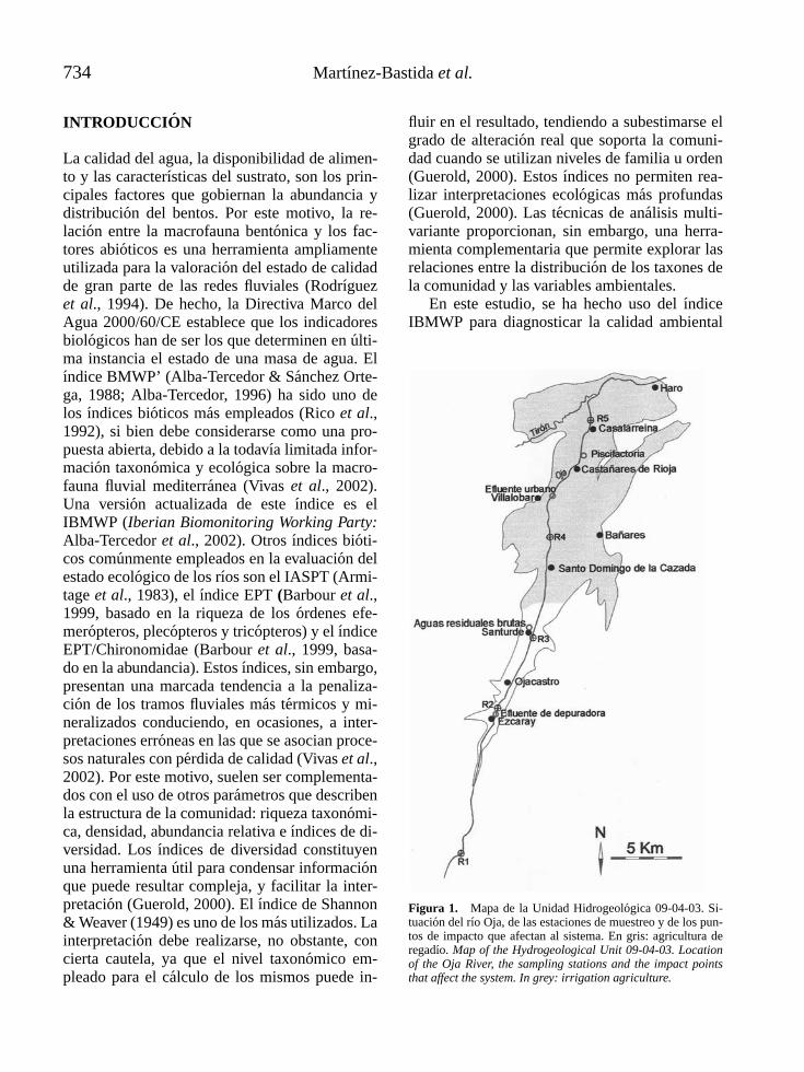
734 Martınez-Bastida et al.
INTRODUCCION
La calidad del agua, la disponibilidad de alimen-to y las caracterısticas del sustrato, son los prin-cipales factores que gobiernan la abundancia ydistribucion del bentos. Por este motivo, la re-lacion entre la macrofauna bentonica y los fac-tores abioticos es una herramienta ampliamenteutilizada para la valoracion del estado de calidadde gran parte de las redes fluviales (Rodrıguezet al., 1994). De hecho, la Directiva Marco delAgua 2000/60/CE establece que los indicadoresbiologicos han de ser los que determinen en ulti-ma instancia el estado de una masa de agua. Elındice BMWP’ (Alba-Tercedor & Sanchez Orte-ga, 1988; Alba-Tercedor, 1996) ha sido uno delos ındices bioticos mas empleados (Rico et al.,1992), si bien debe considerarse como una pro-puesta abierta, debido a la todavıa limitada infor-macion taxonomica y ecologica sobre la macro-fauna fluvial mediterranea (Vivas et al., 2002).Una version actualizada de este ındice es elIBMWP (Iberian Biomonitoring Working Party:Alba-Tercedor et al., 2002). Otros ındices bioti-cos comunmente empleados en la evaluacion delestado ecologico de los rıos son el IASPT (Armi-tage et al., 1983), el ındice EPT (Barbour et al.,1999, basado en la riqueza de los ordenes efe-meropteros, plecopteros y tricopteros) y el ındiceEPT/Chironomidae (Barbour et al., 1999, basa-do en la abundancia). Estos ındices, sin embargo,presentan una marcada tendencia a la penaliza-cion de los tramos fluviales mas termicos y mi-neralizados conduciendo, en ocasiones, a inter-pretaciones erroneas en las que se asocian proce-sos naturales con perdida de calidad (Vivas et al.,2002). Por este motivo, suelen ser complementa-dos con el uso de otros parametros que describenla estructura de la comunidad: riqueza taxonomi-ca, densidad, abundancia relativa e ındices de di-versidad. Los ındices de diversidad constituyenuna herramienta util para condensar informacionque puede resultar compleja, y facilitar la inter-pretacion (Guerold, 2000). El ındice de Shannon& Weaver (1949) es uno de los mas utilizados. Lainterpretacion debe realizarse, no obstante, concierta cautela, ya que el nivel taxonomico em-pleado para el calculo de los mismos puede in-
fluir en el resultado, tendiendo a subestimarse elgrado de alteracion real que soporta la comuni-dad cuando se utilizan niveles de familia u orden(Guerold, 2000). Estos ındices no permiten rea-lizar interpretaciones ecologicas mas profundas(Guerold, 2000). Las tecnicas de analisis multi-variante proporcionan, sin embargo, una herra-mienta complementaria que permite explorar lasrelaciones entre la distribucion de los taxones dela comunidad y las variables ambientales.
En este estudio, se ha hecho uso del ındiceIBMWP para diagnosticar la calidad ambiental
Figura 1. Mapa de la Unidad Hidrogeologica 09-04-03. Si-tuacion del rıo Oja, de las estaciones de muestreo y de los pun-tos de impacto que afectan al sistema. En gris: agricultura deregadıo. Map of the Hydrogeological Unit 09-04-03. Locationof the Oja River, the sampling stations and the impact pointsthat affect the system. In grey: irrigation agriculture.

Calidad ambiental del rıo Oja a partir de macroinvertebrados bentonicos 735
Tabla 1. Frecuencias relativas ( %) de los grupos taxonomicos de la comunidad macrobentonica en cada estacion de muestreo.Relative frequency ( %) of the macroinvertebrate community taxonomic groups at each sampling station.
Cabecera Ezcaray Santurde Santo Domingo Casalarreina
Ephemeroptera 28.17 12.03 13.53 25.69 4.45Plecoptera 4.96 8.42 4.74 0.70 0.25Trichoptera 6.44 0.75 0 0 0.06Coleoptera 8.33 1.05 0.26 0.11 0.20Diptera 24.11 24.66 76.88 65.97 87.94Chironomidae 22.22 22.71 75.63 60.45 83.93Oligochaeta 12.30 43 1.34 6.38 2.54Amphipoda 0 4.06 0.18 0 3.62Isopoda 0 1.65 0.54 0 0.05Ostracoda 4.07 0.90 0.36 0.08 0.14Copepoda 0.20 0.60 0.36 0.43 0.34Turbellaria 0.39 0 0 0 0Hirudinea 0 0.30 0.36 0 0Nematoda 0 0 0 0.22 0Gasteropoda 0 0.45 0 0 0.04
del rıo Oja (La Rioja, Espana). Con la aplicaciondel mismo, se pretende obtener informacion so-bre el grado de alteracion en que se encuentranlos distintos tramos del rıo. Los ındices EPT (ri-queza de familias) y EPT/Chironimidae (abun-dancia) han sido empleados con el mismo fin, co-mo informacion complementaria, puesto que sonındices de tipo cuantitativo, ofrecen una visionrapida del estado del sistema y muestran algunascaracterısticas de la comunidad (riqueza de taxo-nes indicadores y relaciones de dominancia entrealgunos de los principales ordenes del sistema).Se ha estudiado, asimismo, la evolucion de la es-tructura de la comunidad a lo largo del gradientelongitudinal del rıo, mediante el uso de ındicesde abundancia relativa, riqueza, densidad y di-versidad de Shannon-Weaver. Por ultimo, se haanalizado la relacion entre los factores abioticosy la estructura de la comunidad macrobentonicadel rıo, mediante el uso de tecnicas multivarian-tes con el fin de identificar los principales facto-res ambientales que influyen sobre la comunidad.
MATERIAL Y METODOS
Area de estudio
El rıo Oja (La Rioja, Espana) nace en la Sierrade la Demanda (Ezcaray), a 1880 metros de
altitud, y desemboca en el Tiron, a 480 metros(pertenecientes ambos a la cuenca del Ebro).Tiene una longitud de 47 km y una pendientemedia del 29 % (Zaldıvar, 1994), lo que favoreceun flujo rapido del agua. El sustrato geologicosobre el que discurre el rıo y su acuıfero aluvial(perteneciente a la Unidad Hidrogeologica 09-04-03), lo conforman depositos del Cuaternario(coluviales, aluviales, terrazas aluviales, terrazasbajas y conos de pie de monte), con una litologıade gravas gruesas aluviales, gravas polıgenicas,arenas y limos (Instituto Geologico y Minerode Espana, 1985). El regimen hidrologico esde tipo pluvionival. La Unidad Hidrogeologicaocupa una superficie aproximada de 148.5 km2.
El rıo Oja recibe, a lo largo de su curso, algu-nas descargas de efluentes residuales procedentesde pequenos nucleos urbanos e industriales (Fig.1). Tal es el caso de la estacion depuradora deEzcaray, que trata agua residual de tipo mixto, yvierte su efluente sobre el rıo. Las aguas residua-les brutas de Santurde se infiltran directamente enel acuıfero y las de Villalobar se incorporan al rıoa traves de uno de un arroyo tributario. En las pro-ximidades de Castanares existe una piscifactorıa.Por otra parte, la zona media y baja de la cuen-ca esta destinada a la agricultura de regadıo, quefavorece la lixiviacion de los compuestos nitro-genados empleados como fertilizantes y su trans-

736 Martınez-Bastida et al.
porte hacia las masas de agua. El agua de rie-go se obtiene, principalmente, de la explotaciondel acuıfero aluvial, lo que propicia que el ni-vel freatico experimente grandes oscilaciones alo largo del ano, llegando incluso a desaparecerel agua del cauce durante el periodo estival. De-bido a la irregularidad del caudal, existe riesgode crecidas, generalmente durante la primavera.A principios del mes de mayo del 2003, semanasantes del muestreo, las fuertes lluvias provocaronel desbordamiento de las aguas, inundando tie-rras de cultivo y carreteras.
Metodologıa
La campana de muestreos se llevo a cabo durantela primavera del ano 2003. Se establecieron cin-co estaciones de muestreo a lo largo del recorridodel rıo, tendiendo en cuenta los puntos que eranobjeto de algun tipo de perturbacion conocida, aexcepcion de la primera estacion (R1), situadaen cabecera. La segunda estacion (R2), se loca-lizo a unos cien metros aguas abajo del vertidodel efluente residual procedente de la depuradorade Ezcaray. El resto de las estaciones se ubica-ron en Santurde (R3), dos kilometros mas abajode Santo Domingo de la Calzada (R4) y en Ca-salarreina (R5, proxima a su confluencia con elTiron), areas de intensa actividad agrıcola (Fig.1). En cada estacion se realizaron mediciones insitu de temperatura del agua, pH, potencial re-dox (ORP), conductividad electrica y porcenta-je de saturacion de oxıgeno ( % DO), medianteun sistema multiparametrico portatil conectado amultisonda y kit pH/re-dox (ORP), (modelo YSI556). Asimismo, se recogieron muestras simplespara la determinacion de la demanda quımica deoxıgeno (DQO) y las concentraciones de nitra-tos y fosfatos. La DQO se determino mediantela tecnica del dicromato potasico (APHA, 1998).Los aniones se determinaron mediante cromato-grafıa ionica (IC). El caudal se estimo como elproducto del area de la seccion transversal del rıoy la velocidad de la corriente (correntımetro).
El muestreo de los macroinvertebrados serealizo mediante el uso de un Surber 30 × 30cm (250 µm de luz de malla), y una red de de-riva, situada a contracorriente durante un periodo
de 30 minutos. Se tomaron un mınimo de 6 y unmaximo de 12 muestras en cada estacion depen-diendo de la anchura del rıo (mas la de la red dederiva), distribuidas a lo largo de la seccion trans-versal del cauce. Cuando la heterogeneidad am-biental de la seccion requerıa incorporar algunamas, ası se hacıa. Las muestras de macroinver-tebrados fueron conservadas inicialmente en for-mol y posteriormente separadas y determinadashasta el nivel taxonomico de familia, mediante eluso de claves generales (p.e. Tachet et al., 2002).
La evaluacion de la calidad biologica del sis-tema fluvial se realizo mediante la aplicacion delındice IBMWP (Alba-Tercedor et al., 2002) encada una de las estaciones muestreadas. Tambiense hizo uso del ındice EPT riqueza (basado en fa-milias de efemeropteros, plecopteros y tricopte-ros) y el ındice EPT/Chironomidae (basado enabundancia), como informacion complementaria.Para el analisis de la estructura de la comunidadse determinaron los parametros de abundanciarelativa, densidad (individuos/m2), riqueza y elındice de diversidad de Shannon & Weaver (H′)a partir de las familias. Por ultimo, se utilizo elanalisis de componentes principales (ACP) y elanalisis de correspondencias (AC) del programaStatistica 6.0 (StatSoft, 2003), para estudiar la re-lacion entre las variables ambientales y la estruc-tura de la comunidad macrobentonica. El anali-sis de componentes principales se realizo a par-tir de la matriz formada por las siguientes varia-bles: pH, temperatura, caudal, porcentaje de sa-turacion de oxıgeno, potencial redox, conducti-vidad, DQO, nitratos, fosfatos e ındices IBMWPy H′. Se realizo una normalizacion de las varia-bles previa al analisis, mediante transformacionlogarıtmica. El analisis de correspondencias, serealizo a partir de la matriz de abundancias de lasfamilias de macroinvertebrados. En el diagramade ordenacion, solo se representaron los taxonesque alcanzaron valores significativos.
RESULTADOS
Se han identificado un total de 18 ordenes y 53familias de macroinvertebrados acuaticos (masinformacion Valladolid et al., 2006). Los gru-

Calidad ambiental del rıo Oja a partir de macroinvertebrados bentonicos 737
Tabla 2. Valores de IBMWP, rango de calidad, estado ecologico, nivel de calidad y colores asociados en cada estacion de muestreo.IBMWP values, quality range, ecological state, quality level and associated colours at each station.
Estaciones IBMWP Rango Estado ecologico Calidad Color
Cabecera 197 >150 Muy bueno Aguas muy limpias AzulEzcaray 135 150-120 Bueno Aguas limpias AzulSanturde 118 101-120 Bueno Aguas no contaminadas o alteradas de modo sensible AzulSanto Domingo 106 101-120 Bueno Aguas no contaminadas o alteradas de modo sensible AzulCasalarreina 99 61-100 Aceptable Son evidentes algunos efectos de la contaminacion Verde
pos con mayor abundancia y frecuencia de apa-ricion fueron dıpteros, seguido de efemeropteros(Tabla 1). Desde el punto de vista taxonomico,los ordenes mejor representados fueron nueva-mente dıpteros, con 14 familias, y tricopteros,
Figura 2. Proyeccion de las variables ambientales y las esta-ciones de muestreo sobre el plano definido por los ejes 1 y 2 delanalisis de componentes principales. Projection of the environ-mental variables and sampling stations on the axis 1 and 2 ofthe principal components analysis plane.
con 8 familias, si bien estos ultimos presenta-ron una escasa abundancia y se localizaron casiexclusivamente en la estacion de cabecera. Losefemeropteros fueron dominantes en la cabece-ra, mientras que el grupo oligoquetos lo fue enla estacion de Ezcaray. En el resto de estaciones,los dıpteros, a traves de la familia Chironomi-dae presentaron las mayores abundancias relati-vas, segun se aprecia en la Tabla 1.
En la Tabla 2 se presentan los valores del ındi-ce IBMWP. Se observa un estado ecologico muybueno en la estacion de cabecera. En el resto delas estaciones el estado ecologico es bueno, a ex-cepcion de la estacion de Casalarreina (R5), quese encuentra en el umbral que separa las aguasclasificadas como buenas de las aceptables. Seaprecia, asimismo, una disminucion del valor delındice conforme aumenta la distancia respecto ala cabecera, especialmente en Ezcaray, debido alefecto del efluente de la depuradora.
En la Tabla 3 se presentan los valores de losındices biologicos EPT riqueza y EPT/Chirono-midae, y los correspondientes a la riqueza de fa-milias, abundancia total e ındice de diversidad deShannon-Weaver. En los ındices EPT riqueza yEPT/Chironomidae se observan valores bajos enlas tres ultimas estaciones, con dominancia deltaxon Chironomidae respecto a los grupos de efe-meropteros, plecopteros y tricopteros. La riquezade familias e ındice de diversidad de Shannon-Weaver, presentan una tendencia a disminuir pro-gresivamente en el sentido longitudinal del rıo.En el parametro de densidad se observa, por elcontrario, un aumento progresivo a lo largo delcurso del rıo (salvo en Ezcaray).
Los valores de las variables fısico-quımicaspara cada estacion se muestran en la Tabla 4. Seobserva un incremento progresivo de la concen-

738 Martınez-Bastida et al.
Figura 3. Diagrama de ordenacion del analisis de correspon-dencia (ejes 1 y 2) de las estaciones de muestreo y las fami-lias de macroinvertebrados. Correspondence analysis ordina-tion diagram (axes 1 and 2) with sampling stations and macro-invertebrate families.
tracion de nitrato, la DQO, la temperatura y laconductividad a lo largo del gradiente longitu-dinal del rıo. El caudal, sin embargo, manifies-ta otra tendencia, presentando en Santo Domingoun valor menor a los observados en las estacionessituadas aguas arriba. En las estaciones de Ezca-ray (R2) y Santurde (R3), bajo el efecto del ver-
tido de efluentes residuales, se observaron altasconcentraciones de ion fosfato.
En la figura 2 se muestra la proyeccion de lasvariables ambientales y las estaciones de mues-treo, sobre el plano definido por los dos primerosejes del analisis de componentes principales. Losautovalores asociados al primer y segundo ejeson, respectivamente, 7.4 y 1.9 y explican en con-junto un 84.8 % de la varianza. El eje 1 (67.4 %de la varianza) presenta una alta correlacion ne-gativa con el pH, la conductividad, los nitratos,la DQO y la temperatura, y correlacion positi-va con el potencial redox, porcentaje de satura-cion de oxıgeno, el ındice H′ y el ındice IBMWP.Las estaciones de muestreo aparecen ordenadassobre el eje 1 segun su disposicion en el senti-do longitudinal del rıo, en concordancia con elgradiente de calidad. El eje 2 (17.4 %), muestrauna correlacion negativa con los fosfatos y, enmenor medida, con el caudal, y diferencia a Ez-caray y Santurde del resto de estaciones, hechoatribuible al efecto del aporte de fosfatos por ladepuradora de Ezcaray.
En el analisis de correspondencias (Fig. 3)los autovalores de los dos primeros ejes (0.432y 0.290) explican el 82.2 % de la varianza. Laordenacion de las estaciones en el primer eje(49.2 % de la varianza) separa la estacion deEzcaray (impacto del efluente de la depuradora),representada por los taxones Psychomyidae,Planorbidae, Hydroscaphidae, Eurycerdidae,Naididae y Erpobdellidae. La ordenacion asocia-da al eje 2 (32.99 %) diferencia claramente laestacion de cabecera del resto, hecho que reflejaun cambio importante en la composicion de lacomunidad de macroinvertebrados asociado algradiente longitudinal de calidad (aumento dela salinidad, DQO, temperatura y pH; veaseFig. 2). Los taxones mas representativos de estetramo de cabecera, montanoso, de aguas limpiasmuy poco mineralizadas y temperaturas frıas,son los siguientes: Goeridae, Brachycentridae,Sericostomatidae, Uenoidae (tricopteros), Per-lidae, Chloroperlidae, Capniidae (plecopteros),Blephariceridae (dıpteros) y Planariidae (plana-rias). En el extremo negativo no se apreciaagrupaciones de taxones concretos.

Calidad ambiental del rıo Oja a partir de macroinvertebrados bentonicos 739
Tabla 3. EPT riqueza, EPT/ Chironomidae, riqueza de familias, densidad e ındice de diversidad de Shannon-Weaver (H′) para cadaestacion. EPT richness, EPT/ Chironomidae, families’ richness, density and Shannon-Weaver diversity index (H′) for each station.
Estaciones EPT riqueza (familias) EPT/Chironomidae Riqueza (familias) Densidad (individuos/m2) H′
Cabecera 24 1.64 32 0848 2.37Ezcaray 16 0.85 31 0643 1.91Santurde 09 0.23 27 1091 0.92Santo Domingo 09 0.40 24 3658 1.11Casalarreina 07 0.05 22 4301 0.65
DISCUSION
Los resultados obtenidos tras la aplicacion delındice IBMWP indican que las aguas del Rıo Ojapresentan una muy buena calidad en el tramo altoy una calidad buena en los tramos medio y bajo(Tabla 2). No obstante, las variaciones observa-das en la composicion y estructura de la comu-nidad de macroinvertebrados parecen evidenciaralteraciones locales en determinados puntos delsistema. En la estacion de Ezcaray, el hecho deque los oligoquetos pasen a constituir el grupo ta-xonomico dominante, por delante de efemeropte-ros e incluso dıpteros, puede atribuirse a la in-fluencia del vertido de la depuradora sobre el sis-tema fluvial (Tabla 1). El analisis de componen-tes principales (Fig. 2) separa la estacion de Ez-caray (mayor presencia de ortofosfato procedentede la depuradora), si bien no contamos con datossobre otros posibles contaminantes procedentesdel polıgono industrial que podrıan estar afectan-do a la estructura de la comunidad.
Los bajos valores de los ındices de di-versidad de Shannon, de EPT riqueza y deEPT/Chironomidae en las estaciones del tramomedio y bajo de la cuenca (Tabla 3) parecen indi-car la existencia de un cierto deterioro, con clarodominio de los quironomidos sobre efemeropte-
ros, plecopteros y tricopteros (comunmente aso-ciados a condiciones poco alteradas). La eleva-da proporcion de quironomidos, podrıa tambienexplicarse por los efectos de la crecida que tuvolugar tres semanas antes del muestreo. Existendiversos estudios que hacen referencia al efectodestructor que este tipo de fenomenos naturalestiene sobre las comunidades de macroinvertebra-dos (Morais et al., 2004; Robinson et al., 2004;Rodrıguez et al., 1994; Shieh & Yang, 2000; Vi-tor Cortes et al., 2002; Voelz et al., 2000) debi-do al arrastre de los individuos, que provoca ladesorganizacion y la disminucion del tamano dela comunidad. En estas circunstancias los taxo-nes oportunistas y tolerantes, con un ciclo de vi-da corto, se ven favorecidos en las primeras fasesde recolonizacion y recuperacion. Chironomidae,Simuliidae y Baetidae son algunos de los que pre-sentan una recuperacion mas rapida ante fenome-nos de este tipo (Robinson et al., 2004). El escasotiempo de recuperacion transcurrido desde la cre-cida hasta el momento del muestreo, explicarıatambien los bajos valores de diversidad y riquezadetectados en los tramos medios y bajos. Pupilli& Puig (2003) observaron en un estudio en el rıoMataranya (perteneciente a la cuenca del Ebro)un descenso de mas del 97 % en las densidadesde los taxones tras una intensa crecida. Voetz et
Tabla 4. Parametros fısico quımicos en cada estacion. Physico chemical-parameters at each station.
Estaciones Temperatura (◦C) Caudal PH Conductividad ORP (mV) DO ( %) NO−3 (mg/l) PO–34 (mg/l)
(m3/s) (µµµs/cm)
Cabecera 07.02 0.82 5.63 012 204.6 128.2 00.0 0.0Ezcaray 11.88 1.62 7.22 109 197.0 125.0 01.9 0.3Santurde 11.51 1.86 7.44 135 042.8 127.2 02.9 0.3Santo Domingo 16.81 0.37 8.01 210 017.0 128.6 07.3 0.0Casalarreina 15.28 1.72 7.54 216 011.8 102.8 16.9 0.0

740 Martınez-Bastida et al.
al. (2000) realizaron observaciones similares enel rıo Colorado, constatando que la comunidadde macroinvertebrados recuperaba los niveles dedensidad y riqueza previos en un tiempo que va-riaba de unos meses a un ano. Diversos estudioscoinciden en otorgar a la comunidad de macroin-vertebrados una gran capacidad de recuperacionante episodios de crecidas e inundaciones (Gib-bins et al., 2001; Morais et al., 2004; Voelz et al.,2000), senalando los escasos cambios estructura-les en la comunidad a una escala temporal am-plia (a pesar de la recurrencia de eventos natura-les de este tipo y de manifestar una cierta variabi-lidad a corto plazo tras los mismos). La adecua-da comprension del funcionamiento del sistemay el discernimiento entre los efectos inducidospor factores naturales y antropicos, requieren eldesarrollo de estudios a largo plazo (Naiman etal., 1995). Es necesario, por tanto, realizar cam-panas de muestreo en el Oja a escala estacionalpara profundizar en estos aspectos.
El gradiente de calidad observado en el rıoOja a lo largo del perfil longitudinal parece res-ponder a una combinacion de los efectos de-rivados de las actividades antropicas (actividadagrıcola y vertidos de efluentes residuales) y lasvariaciones que de forma natural experimentanlos factores ambientales del sistema. Estos fac-tores, que parecen afectar a la distribucion y es-tructura de la comunidad de macroinvertebradosen el Oja, son comparables a los observados porVivas et al. (2002) en su estudio de los rıos medi-terraneos de las principales cuencas espanolas. Asu vez, se aprecia una concordancia con las ob-servaciones de Shiegh & Yang (2000) en un arro-yo de montana en Taiwan situado en un area degran actividad agrıcola. Shieh & Yang apreciaronque la aplicacion de fertilizantes nitrogenados yotras sustancias quımicas, explicaban los eleva-dos valores de conductividad, concentracion denitrato y dureza detectados en el rıo y a su vezlos bajos valores de densidad, riqueza y diversi-dad taxonomica obtenidos. Rodrigues Capıtulo etal. (2001) tambien observaron en rıos de Argen-tina una progresiva sucesion, aguas abajo, de ta-xones sensibles a la contaminacion por otros mastolerantes (quironomidos y oligoquetos), ante lamayor presencia de contaminantes y nutrientes
procedentes de la actividad agrıcola y el verti-do de efluentes residuales en las estaciones dela zona baja del rıo. El enriquecimiento organi-co y salino moderado observado en el Oja, favo-rece la instalacion de una comunidad mas tole-rante a la mineralizacion y carga organica, quecontribuye a diferenciar la zona mas humaniza-da de la zona de cabecera, como se puede apre-ciar en la segunda dimension del analisis de co-rrespondencias (Fig. 3). Los taxones caracterısti-cos de aguas de cabecera (Goeridae, Brachycen-tridae, Sericostomatidae, Uenoidae, Blepharice-ridae, Perlidae, Capniidae) son sustituidos en lostramos medios y bajos por un amplio grupo de ta-xones mas tolerantes como Chironomidae, Baeti-dae, Simuliidae, Gammaridae, Lumbricidae, Ce-ratopogonidae y Lumbriculidae.
El rıo presenta una buena capacidad de auto-depuracion, debido a las fuertes pendientes quesuelen dominar la mayor parte de su perfil lon-gitudinal, y al caracter puntual y reducido de losimpactos. No obstante, debe tenerse en cuenta elposible efecto de estos impactos durante el perio-do estival, especialmente, considerando que en elrıo Oja las variaciones de caudal asociadas a laestacionalidad natural del sistema son acentua-das, por la presion derivada de la explotacion delacuıfero aluvial con fines agrıcolas. La menor ca-pacidad de lavado y de dilucion del sistema, y lamayor evaporacion tienden a intensificar duranteeste periodo los efectos de la alteracion antropi-ca y a evidenciar los procesos de contaminacion(Vivas et al., 2002).
Las comunidades de los rıos estan fuertemen-te asociadas a estas variaciones del flujo del sis-tema (Armitage et al., 2001; Basaguren et al.,1996; Caruso, 2002; Fleituch, 2003, Gibbins etal., 2001; Habidija et al., 2003; Wright & Sy-mes, 1999; Rodrıguez et al., 2002). El patrongeneral observado en rıos mediterraneos y otrossistemas similares sometidos a variaciones esta-cionales, se refleje en un predominio de taxonesmas tolerantes a la contaminacion (Morais et al.,2004; Rodriguez et al., 1994; Wood et al., 2000).Las especies reofilas y los filtradores reducen sudensidad, mientras que los detritıvoros la aumen-tan (Extence, 1981; Pearson, 1984). Ası mismo,plecopteros, efemeropteros y tricopteros pierden

Calidad ambiental del rıo Oja a partir de macroinvertebrados bentonicos 741
importancia ante la progresiva dominancia de losgrupos de odonatos, heteropteros, coleopteros ydıpteros (Rieradevall et al., 1999; Vivas et al.,2003). Se ha observado, asimismo, una tenden-cia a la disminucion de los parametros de rique-za, densidad y abundancia de la comunidad (Ca-ruso, 2002), si bien, existen estudios que mues-tran lo contrario (Morais et al., 2004; Rieradevallet al. 1999) debido a la mayor disponibilidad dealimento (alta diversidad de algas verdes filamen-tosas y diatomeas) y diversidad de nichos que secrean en algunos casos (Morais et al., 2004). Enel rıo Oja algunos tramos llegan a secarse, lo cualpuede intensificar los efectos sobre la comunidadmacrobentonica. Algunos autores (Caruso, 2002;Delucchi, 1989) no obstante, indican que ciertostaxones han desarrollado mecanismos para per-manecer durante ese periodo de gran estres hıdri-co, en formas de resistencia en el sustrato. En lostramos no afectados por contaminacion, como lacabecera, las variaciones de temperatura podrıanexplicar la ausencia de familias estenotermasque habitualmente suelen encontrarse en la zonarithron (como Heptageniidae).
Como conclusion general puede decirse que elsistema se encuentra en un buen estado de conser-vacion, ya que los impactos son de reducida in-tensidad y el rıo presenta una buena capacidad deautodepuracion, si bien merece la pena mencio-nar el efecto de fenomenos naturales como sonlas avenidas, y el posible efecto de los estiajes.
AGRADECIMIENTOS
Este trabajo de investigacion se esta financiandoa traves del Proyecto del Plan Nacional de I+D(REN2002-02550). La Union de Agricultoresy Ganaderos-Coordinadora de Agricultores yGanaderos (UAGR- COAG) apoya el desarrollode la investigacion mediante un ContratoTecnologico (ref. 2003/672).
La Consejerıa de Educacion de la Comunidadde Madrid y el Fondo Social Europeo (F.S.E.)participan mediante la financiacion de una becade Formacion de Personal Investigador.
BIBLIOGRAFIA
ALBA-TERCEDOR, J. & A. SANCHEZ-ORTEGA.1988. Un metodo rapido y simple para evaluar lacalidad biologica de las aguas corrientes basado enel de Hellawell (1978). Limnetica, 4: 51-56.
ALBA-TERCEDOR, J. 1996. Macroinvertebradosacuaticos y calidad de las aguas de los rıos.IV Simposio del Agua en Andalucıa (SIAGA),Almerıa, Espana: 203-213.
ALBA-TERCEDOR, J., P. JAIMEZ-CUELLAR, M.ALVAREZ, J. AVILES, N. BONADA, J. CA-SAS, A. MELLADO, M. ORTEGA, I. PARDO,N. PRAT, M. RIERADEVALL, S. ROBLES, C. E.SAINZ-CANTERO, A. SANCHEZ-ORTEGA, M.L. SUAREZ, M. TORO, M. R. VIDAL-ABARCA,S. VIVAS & C. ZAMORA-MUNOZ. 2002. Ca-racterizacion del estado ecologico de rıos medi-terraneos ibericos mediante el ındice IBMWP (an-tes BMWP’). Limnetica, 21: 175-185.
APHA. 1998. Standard methods for the examination ofwater and wastewater, 20th ed. American PublicHealth Association, American Water Works Associa-tion & Water Environment Federation. USA. 1134 pp.
ARMITAGE P. D., D. MOSS, J. F. WRIGHT & M.T. FURSE. 1983. The performance of a new bio-logical water quality score system based on ma-croinvertebrates over a wide range of unpollutedrunning-water sites. Wat. Res., 17: 333-347.
ARMITAGE, P. D., K. LATTMANN, N. KNEEBO-NE & I. HARRIS. 2001. Bank profile and structureas determinants of macroinvertebrate assemblages-seasonal changes and management. Regul. Rivers:Res. Mgmt., 17: 543–556.
BARBOUR, M. T., J. GERRITSEN, B. D. SNYDER& J. B. STRIBLING. 1999. Rapid BioassessmentProtocols or Use in Streams and Wadeable Rivers:Periphyton, Benthic Macroinvertebrates and Fish.U.S. Environmental Protection Agency, EPA-891-B99-002. Washington D.C. 339 pp.
BASAGUREN, A., A. ELOSEGUI, J. POZO. 1996.Changes in the trophic structure of benthic macroin-vertebrate communities associated with food avai-lability and stream flow variations. InternationaleReveu Der Gesamten Hydrobiologie, 81: 79-91.
CARUSO, B. S. 2002. Temporal and spatial patterns ofextreme low flows and effects on stream ecosystemsin Otago, New Zealand. J. Hydrol., 257: 115-133.
COIMBRA, C. N., M. A. S. GRACA & R. M. COR-TES. 1996. The effects of a basic effluent on ma-
742 Martınez-Bastida et al.
croinvertebrate community structure in a tempo-rary Mediterranean river. Env. Poll., 94: 301-307.
DELUCHI, C. M. 1989. Movement patterns of inver-tebrates in temporary and permanent streams. Oe-cologia, 78: 199-207.
EXTENCE C. A. 1981. The effect of drought onbenthic invertebrate communities in a lowland ri-ver. Hydrobiologia, 83: 217–224.
FLEITUCH, T. 2003. Structure and Functional Orga-nization of Benthic Invertebrates in a RegulatedStream. Internat. Rev. Hydrobiol., 88: 332–344
GIBBINS, C. N., C. F. DILKS, R. MALCOLM, C.SOULSBY & S. JUGGINS. 2001. Invertebrate com-munities and hydrological variation in Cairngormmountain streams.Hydrobiologia,462:205-219.
GUEROLD, F. 2000. Influence of taxonomic deter-mination level on several community indices. Wat.Res., 34: 487-492.
HABIDIJA I., I. RADANOVIC, B. PRIMC-HABDI-JA, R. MATONICKIN, M. KUCINIC. 2003. Riverdischarge regime as a factor affecting the changesin community and functional feeding group com-position of macroinvertebrates on a cobble substra-te in the Sava river. Biologia, 58: 217-229.
INSTITUTO GEOLOGICO Y MINERO DE ES-PANA, 1985. Plano Hidrogeologico no 1, Investi-gacion hidrogeologica del cuaternario del rıo Gle-ra (La Rioja). Clave: ZP-1490. Escala 1:50.000.
MORAIS, M., P. PINTO, P. GUILHERME, J. RO-SADO & I. ANTUNES. 2004. Assessment of tem-porary streams: the robustness of metric and multi-metric indices under different hydrological condi-tions. Hydrobiologia, 516: 229-249.
NAIMAN, R. J., J. J. MAGNUSON, D. M. MCK-NIGHT & J. A. STANFORD. 1995. The FreshwaterImperative. Island Press. Washington, D.C. 165 pp.
PEARSON, R. G. 1984. Temporal changes inthe composition and abundance of the macro-invertebrate communities of the River Hull. Arch.Hydrobiol., 100: 273–298
PUPILLI, E. & M. A. PUIG. 2003. Effects of a ma-jor flood on the mayfly and stonefly populations ina Mediterranean stream (Matarranya Stream, EbroRiver basin, North East of Spain). Research Upda-te on Ephemeroptera & Plecoptera. E. Gaino (ed.):381-389. University of Perugia, Perugia.
RICO, E., A. RALLO, M. A. SEVILLANO & M. I.ARRETXE. 1992. Comparison of several biologi-cal indices based on river macroinvertebrate bent-hic community for assessment of running waterquality. Ann. Limnol., 28: 147-156.
RIERADEVALL, M., N. BONADA, N. PRAT. 1999.Community structure and water quality in the Me-diterranean streams of a natural park (St. Llorencdel Munt, NE Spain). Limnetica, 17: 45-56.
ROBINSON, C. T., U. R. S. UEHLINGER & M. T.MONAGHAN. 2004. Stream ecosystem responseto multiple experimental floods from a reservoir.River Res. Applic., 20: 359-377.
RODRIGUEZ, S. E., C. FERNANDEZ-ALAEZ, M.FERNANDEZ-ALAEZ & E. BECARES. 1994.Caracterizacion de la comunidad de macroinverte-brados de la cuenca alta del rıo Cares. Limnetica,10: 93-100.
RODRIGUES CAPITULO, A., M. TANGORRA &C. OCON. 2001. Use of benthic macroinvertebra-tes to assess the biological status of Pampean streamsin Argentina. Aquatic Ecology, 35: 109-119.
SHANNON, C. E. & W. WEAVER. 1949. The Mat-hematical Theory of Communication. Univ. of Illi-nois Press. Urbana. 119 pp.
SHIEH, S. & YANG, P. 2000. Community Structureand functional Organization of Aquatic Insects in anAgricultural Mountain Stream of Taiwan: 1985-1986and 1995-1996. Zoological Studies, 39: 191-202.
STATSOFT, INC. 2003. Statistica for Windows. Tul-sa, Oklahoma.
TACHET,H.,P.RICHOUX,M.BOURNAUD&P. US-SEGLIO-POLATERA. 2002. Invertebres d’eau dou-ce. Systematique, biologie, ecologie. CNRS ed. Parıs.
VALLADOLID, M., J. J. MARTINEZ-BASTIDA, M.ARAUZO & C. GUTIERREZ. 2006. Abundanciay biodiversidad de los macroinvertebrados del rıoOja (La Rioja, Espana). Limnetica, 25: 133-140.
VIVAS, S., J. CASAS, I. PARDO, S. ROBLES, N.BONADA, A. MELLADO, N. PRAT, J. ALBA-TERCEDOR, M. ALVAREZ, M. R. VIDAL.-ABARCA, C. ZAMORA-MUNOZ & G. MOYA.2002. Aproximacion multivariante en la explora-cion de la tolerancia ambiental de las familias demacroinvertebrados de los rıos mediterraneos delproyecto GUADALMED. Limnetica, 21: 149-173.
VITOR CORTES, R. M., M. T. FERREIRA, S. V.OLIVEIRA & D. OLIVEIRA. 2002. Macroinver-tebrate community structure in a regulated riversegment with different flow conditions. River Res.Applic., 18: 367-382.
VOELZ, N. J., S. H. SHIEH & J. V. WARD. 2000.Long-term monitoring of benthic macroinvertebra-te community structure: a perspective from a Co-lorado river. Aquatic Ecology, 34: 261–278.

Calidad ambiental del rıo Oja a partir de macroinvertebrados bentonicos 743
WOOD, P. G., M. D. AGNEW Y G. E. PETTS. 2000.Flow variations and macroinvertebrate communityresponses inasmallgroundwater-dominatedstreaminsouth-eastEngland.Hydrol.Process.,14:3133-3147.
WRIGHT, J. F. & K. L. SYMES. 1999. A nine-year
study of the macroinvertebrate fauna of a chalkstream. Hydrol. Process., 13: 371-385.
ZALDIVAR, C. 1994. Atlas de distribucion de lospeces de la Comunidad Autonoma de La Rioja.Zubia Monografico, 6: 71-102.


Limnetica, 25 (3-4): xx-xx (2006)Limnetica, 25 (3): 745-752 (2006)c© Asociacion Espanola de Limnologıa, Madrid. Spain. ISSN: 0213-8409
Abundancia y biodiversidad de los macroinvertebrados del rıo Oja(La Rioja, Espana)
Marıa Valladolid 1,∗, Juan Jose Martınez-Bastida2, Mercedes Arauzo 2 y Carmen Gutierrez3
1 Dep. Biodiversidad y Biologıa Evolutiva, Museo Nacional de Ciencias Naturales (CSIC), c/ Jose GutierrezAbascal, 2. 28006 Madrid.2 Dep. Contaminacion Ambiental Centro de Ciencias Medioambientales (CSIC), c/ Serrano 115 dpdo., 28006Madrid. E-mail: J.J. Martınez: [email protected], M. Arauzo: [email protected] Departamento de Agroecologıa. Centro de Ciencias Medioambientales (CSIC). Serrano 115 dpdo. 28006Madrid. E-mail: [email protected] HolaAutor responsable de la correspondencia: [email protected]
RESUMEN
Abundancia y biodiversidad de los macroinvertebrados del rıo Oja (La Rioja, Espana)
En mayo de 2003 se realizo un estudio sobre la fauna de invertebrados del rıo Oja (La Rioja, Espana), seleccionandose cincopuntos a lo largo de su cauce. Se observa una disminucion de la diversidad desde los tramos mas altos hasta los mas bajos,ası como un aumento de la abundancia total, representada por unas pocas especies. En los tramos altos dominan Tricopteros,Plecopteros y Efemeropteros, mientras que en los tramos medios-bajos los Tricopteros practicamente desaparecen, siendo losDıpteros, Crustaceos y ciertas especies de Efemeropteros los principales representantes.
Palabras clave: Macroinvertebrados, diversidad, rıo Oja.
ABSTRACT
Abundance and biodiversity of macroinvertebrates of the Oja River (La Rioja, Espana)
During May 2003 a study on the aquatic macroinvertebrate fauna from the Oja River (La Rioja, Spain) was carried outin five selected points along the river. A decrease in diversity from upstream to downstream stretches is observed, as wellas an increase in the total abundance, represented by a few species. In the upstream stretches, the dominant groups wereTrichoptera, Plecoptera, and Ephemeroptera, while in the middle and downstream stretches, Trichoptera almost disappear,being Diptera, Crustacea and certain Ephemeroptera the most abundant taxa.
Keywords: Macroinvertebrates, diversity, Oja River.
INTRODUCCION
La Rioja y su entomofauna acuatica ha sido ob-jeto de estudio desde principios del siglo pasado,debido sobre todo a los trabajos de Navas (p.e.Navas, 1914, 1917a y b), en zonas muy concretasde la region, como Ortigosa, Valvanera y la Sierrade Cameros. Mas recientemente, Garcıa de Jalon(1982), en su zoogeografıa de tricopteros, publicauna relacion de especies encontradas en los rıosIregua y Najera. Por otra parte, hemos observa-
do una escasez de literatura referida al rıo Oja ensı, encontrando por el momento unicamente unartıculo sobre los coleopteros acuaticos del Siste-ma Iberico en la que aparece, entre otros, este rıo(Valladares et al., 2000).
El presente trabajo quiere ser una contribu-cion al conocimiento de la fauna acuatica de in-vertebrados de La Rioja, poco estudiada en mu-chos aspectos y posiblemente vulnerable, debidoal gran desarrollo agrıcola de la zona y con la ex-plotacion de los recursos hıdricos como su prin-

746 Valladolid et al.
Tabla 1. Localizacion de los puntos de muestreo y caracterısticas fısico-quımicas de las aguas del rıo Oja. Location of samplingsites and physico-chemical characteristics of the Oja River waters.
Punto UTM Alt. m Ta agua ◦C Cond µµµs/cm Sal. g/l O2 mg/l pH DQO mg/l SS ss mg/l
R-1 30T 496378 4675906 944 7.02 12 0.01 15.57 5.63 1.00 0.80
R-2 30T 499284 4687396 719 11.88 109 0.07 13.50 7.22 1.60 0.40
R-3 30T 502037 4693135 711 11.51 135 0.11 13.86 7.44 2.20 0.53
R-4 30T 503531 4702049 616 16.81 210 0.12 12.46 8.01 4.20 2.33
R-5 30T 507001 4710589 569 15.28 216 0.15 10.28 7.54 12.20 5.20
cipal amenaza. En esta publicacion presentamosla lista de las especies de invertebrados acuaticosque hemos encontrado, su abundancia y diversi-dad, completando la informacion sobre estas co-munidades y su relacion con la calidad del aguaen una segunda publicacion en este mismo nume-ro de la revista (Martınez Bastida et al., 2006).
AREA DE ESTUDIO
El estudio se llevo a cabo en el rıo Oja (La Rio-ja, Espana) (Fig. 1). Este rıo nace en la Sierrade la Demanda (1880 msnm) y desemboca en elrıo Tiron, poco antes de su desembocadura en elEbro, estando su recorrido (47 km) circunscritoıntegramente a la Rioja Alta. De regimen pluvio-nival, este rıo se caracteriza por grandes varia-ciones de caudal entre distintas epocas del ano,debido por una parte a la fuerte pendiente de sucauce, que hace que la escorrentıa sea importan-te, y por otra, a la fuerte utilizacion del acuıferoaluvial para la agricultura intensiva, con impor-tantes extracciones de agua en los momentos demenor caudal (verano).
Se han seleccionado cinco puntos de muestreoa lo largo del rıo: dos de cabecera, R-1, por enci-ma de Posadas, un poco antes de la union del Ojacon el arroyo Ortigal y R-2, en Ezcaray, por deba-jo de los efluentes de la depuradora. Dos puntosen el tramo medio, R-3, Santurde, a la entrada delvalle aluvial, y R-4, Santo Domingo de la Calza-da, en plena zona de regadıo, y un ultimo puntoen el tramo inferior, R-5, Casalarreina, poco an-tes de su union con el rıo Tiron. El tramo medio(R-3 y R-4) aparece seco durante el verano, recu-perando su caudal con la llegada de las lluvias.
MATERIAL Y METODOS
Para la caracterizacion fısico-quımica del agua setomaron por una parte muestras para su analisisen el laboratorio, y por otra se midieron in situuna serie de variables (Ta, O2 disuelto, pH, con-ductividad, salinidad) mediante una sonda multi-paraparametrica YSI 556.
Para el estudio de los invertebrados se toma-ron un numero variable de muestras en cada pun-to (mınimo 6, maximo 12), dependiendo de la an-chura del rıo. Para ello se utilizo un dispositivotipo surber 30 × 30 cm, con una manga de nytalde 250 µm de luz de malla. Al mismo tiempo, secolocaron aguas arriba redes de deriva de 30 × 30cm, 250 µm de luz de malla, durante 30 minutos.Las muestras se fijaron con formol al 4 % tam-ponado con ClNa al 0.9 %. En el laboratorio losorganismos se separaron con una lupa binoculary se determinaron con la maxima resolucion ta-xonomica posible, conservandose en alcohol de70◦. Para la determinacion se utilizaron distintostipos de claves (p.e. Bertrand, 1954; Puig, 1984,Vieira, 2000; Tachet et al., 2003), ası como des-cripciones de ciertas especies.
Se calculo la abundancia de cada grupo ta-xonomico y la abundancia total en cada punto demuestreo, expresada en individuos/m2. La diver-sidad se calculo mediante el ındice de Shannon-Weaver (H′) y el de Pielou (J′).
RESULTADOS
En la Tabla 1 aparecen reflejados algunos resul-tados de las caracterısticas fısico-quımicas delagua. Son aguas limpias, de buena calidad, con

Macroinvetebrados del rıo Oja (La Rioja, Espana) 747
Figura 1. Localizacion del rıo Oja (La Rioja, Espana) y delas estaciones de muestreo. Location of the Oja River (La Rioja,Spain) and the sampling stations.
baja conductividad y buena oxigenacion, bastanteacidas en la cabecera. La relacion entre variablesambientales y el macrobentos se presenta condetalle en Martınez Bastida et al. (2006).
En cuanto a los invertebrados, la Tabla 2 re-coge las abundancias de las especies encontra-das. Los datos mas importantes son la presenciade una posible nueva especie del genero Threm-ma (Trichoptera: Uenoidae), (pendiente de con-firmar, debido a que solo hay un ejemplar), queaparecio en el punto R-1 (cabecera), y la relacionde nuevas citas de tricopteros, plecopteros y co-leopteros para La Rioja, senalados con un asteris-co (Tabla 2). Entre estas destacan especies cita-das como endemicas de Pirineos, como p.e. Iso-perla moselyi (Plecoptera: Perlodidae) (Despax,1936; Aubert, 1963; Puig, 1980) u otras encon-tradas hasta el momento unicamente en el sur pe-ninsular, como Hydropsyche fontinalis (Zamora-Munoz et al., 2002).
En los tramos altos (R-1 y R-2) se obser-va la mayor riqueza de tricopteros, plecopte-ros, efemeropteros y coleopteros, siendo menoren R-2 debido probablemente al vertido de ladepuradora. En ambos puntos hay un total de41 taxa: tricopteros (7 familias), plecopteros (6familias), efemeropteros (5 familias), coleopte-ros (3 familias), dıpteros (8 familias), colembo-los (1 familia), crustaceos (5 ordenes), molus-cos (1 familia), tricladidos (1 familia), hirudıneos(2 familias) y oligoquetos (3 familias). En eltramo medio (R-3 y R-4) encontramos 30 ta-xa: tricopteros (1 familia), plecopteros (4 fa-milias), efemeropteros (5 familias), coleopteros(3 familias), dıpteros (12 familias), colembolos(1 familia), crustaceos (4 ordenes), hirudıneos(1 familia) y oligoquetos (3 familias). Por ulti-mo, en el tramo bajo (R-5) unicamente apare-cen 26 taxa: tricopteros (1 familia), plecopte-ros (1 familia), efemeropteros (4 familias),coleopteros (1 familia), dıpteros (5 familias),colembolos (1 familia), hemıpteros (1 familia),crustaceos (4 ordenes) y oligoquetos (2 familias).
Los efemeropteros que aparecen son princi-palmente Heptagenidos y Betidos, estos ultimostambien muy abundantes en los tramos medios ybajos. En cuanto a los dıpteros, hay una gran va-riedad de familias, siendo predominantes los Qui-

748 Valladolid et al.
Tabla 2. Abundancia (individuos/m2) de los invertebrados recogidos en el mes de Mayo de 2003. D: individuos recogidos en lasderivas. *: nuevas citas para La Rioja. Abundance (individuals/m2) of invertebrates collected in May 2003. D: specimens collected indrift samples. *: new records for La Rioja.
Invertebrados R-1 R-2 R-3 R-4 R-5 Invertebrados R-1 R-2 R-3 R-4 R-5
TRICHOPTERA BaetidaeHydropsychidae Baetis spp. 156 54 135 935 111
Hydropsyche instabilis 26 0 0 0 0 CaenidaeHydropsyche lobata∗ 0 1 0 0 0 Caenis rivulorum 9 0 1 2 19Hydropsyche siltalai 0 2 0 0 0 Caenis gr. macrura 0 3 0 0 11Hydropsyche fontinalis∗ 0 1 0 0 0 COLEOPTERA
Rhyacophilidae ElmidaeRhyacophila obliterata 4 0 0 0 0 Elmis spp. 2 0 0 2 0Rhyacophila martyinovi∗ 2 0 0 0 0 Esolus spp. 76 6 1 0 0Rhyacophila spp. 0 0 0 0 2 Limnius spp. 6 0 0 0 0
Goeridae Oulimnius spp.∗ 0 0 0 D 9Larcasia partita 9 0 0 0 0 Stenelmis spp.∗ 0 0 0 0 D
Brachycentridae HydraenidaeMicrasema minimum∗ 9 0 0 0 0 Hydraena sp. 1∗ D D 0 2 0Micrasema longulum D 0 0 0 0 Hydraena sp. 2∗ D 0 0 0 0
Sericostomatidae HaliplidaeSchizopelex spp. 6 0 0 0 0 Haliplus spp. D 0 0 0 0Sericostoma spp. 7 0 0 0 0 Hydroscaphidae
Uenoidae Hydroscapha spp. 0 1 0 0 0Thremma spp.∗ 2 0 0 0 0 Dytiscidae
Psychomyidae Yola bicarinata∗ 0 0 2 0 0Psychomyia pusilla 0 1 0 0 0 Agabus spp. 0 0 D 0 0
Hydroptilidae DIPTERAStactobia spp.∗ 0 0 0 D 0 Psychodidae
PLECOPTERA Psychoda spp. 0 0 0 2 7Perlidae Pericoma spp. D 0 1 2 0
Dinocras cephalotes 22 1 0 0 0 BlephariceridaePerlodidae Blepharicera fasciata 2 0 0 0 0
Isoperla moselyi∗ 0 13 7 6 0 Simuliidae 2 10 6 183 33Isoperla spp. 2 0 0 0 0 CeratopogonidaeHemimelaena flaviventris 0 0 0 6 0 Palpomia spp. 0 1 6 0 2
Chloroperlidae ChironomidaeSiphonoperla torrentium 7 0 1 0 0 Tanypodinae 30 31 61 11 4
Taeniopterygidae ChironominaeRhabdiopteryx thienemanni∗ 6 1 0 0 0 Tanytarsini 111 4 18 54 28Brachyptera spp. 0 40 44 10 11 Chironomini 0 12 4 19 0Taeniopteryx shoenemundi∗ 0 0 0 2 0 Orthocladiinae 83 104 761 2151 3733
Nemouridae LimoniidaeProtonemura spp. 7 1 D 0 0 Dicranota spp. 4 1 0 5 0Nemoura spp. D 0 1 2 0 Antocha vitripennis D 0 0 0 0
Capniidae Stratiomyidae 0 0 0 2 0Capnia spp. 6 0 0 0 0 Empididae
EPHEMEROPTERA Hemerodromia spp. 7 1 1 3 0Heptageniidae Atalanta spp. 0 0 0 5 0
Ecdyonurus forcipula/angelieri 4 0 0 0 0 Dolichopodidae 0 0 0 2 0Ecdyonurus lateralis 0 0 1 0 0 Rhagionidae 0 0 0 D 0Ecdyonurus spp. 2 0 0 0 0 AthericidaeRhitrogena sp. 1 31 15 7 0 2 Atherix spp. 4 0 0 0 0Rhitrogena sp. 2 9 0 0 0 0 Atrichops spp. 0 0 0 0 2Epeorus torrentium/sylvicola 2 0 0 0 0 Tabanidae 0 0 D 0 0

Macroinvetebrados del rıo Oja (La Rioja, Espana) 749
Tabla 2 (cont.)
Invertebrados R-1 R-2 R-3 R-4 R-5 Invertebrados R-1 R-2 R-3 R-4 R-5
Epeorus spp. 0 1 0 0 0 SyrphidaeHeptagenia spp. 6 1 0 2 0 Myiatropa spp. 0 0 D 0 0
Ephemerellidae EphydridaeSerratella ignita 61 5 7 11 50 Psilopa spp. 0 0 1 D 0
Leptophlebiidae HEMIPTERAHabrophlebia 0 0 D 0 D Corixidae 0 0 0 0 2S.I. 4 1 0 0 0
COLLEMBOLA NEMATODA 0 D 0 8 0Especie 1 D 1 D 2 4 TURBELLARIAEspecie 2 D 0 0 0 D TRICLADIDAARACHNIDA PlanariidaeActimedida 111 12 16 13 9 Polycelis tenuis 4 0 0 0 0BRANCHIOPODA HIRUDINEAANOMOPODA ARHYNCHOBDELLIDAEurycercidae Erpobdellidae
Alona spp. 0 1 0 0 0 RHYNCHOBDELLIDAChydorus spp. 0 D 0 0 0 Glossiphonidae 0 0 4 0 0
OSTRACODA 41 6 4 3 6 OLIGOCHAETACOPEPODA 2 4 4 16 15 OPISTHOPORAMALACOSTRACA LumbricidaeAMPHIPODA Eiseniella tetraedra 0 1 3 0 6Niphargidae 0 26 2 0 76 LUMBRICULIDAGammaridae Lumbriculidae 109 13 10 219 104
Echinogammarus spp. 0 1 0 0 81 TUBIFICIDAISOPODA NaididaeAsellidae 0 11 6 0 2 Nais spp. 15 269 1 17 0GASTROPODA Specaria-Piguetiella 0 3 0 0 0BASOMMATOPHORA Dero spp. 0 0 1 0 0Planorbidae 0 1 0 0 0
Figura 2. Abundancia total (individuos/m2) y diversidad delos macroinvertebrados del rıo Oja (Mayo 2003). A: abundan-cia, H′: ındice de diversidad de Shannon-Weaver, J′: ındice dePielou. Total abundance (individuals/m2) and diversity of ma-croinvertebrates of the Oja River (May 2003). A: abundance,H′: Shannon-Weaver index, J′: Pielou index.
ronomidos, aunque la abundancia de las distintassubfamilias y tribus varıa en los distintos puntos,p.e. los Tanytarsini (Chironominae) son mayori-tarios en R-1, mientras que los Orthocladinae loson en el resto.
Los crustaceos tambien tienen buena re-presentacion, con branquiopodos, ostracodos,copepodos, isopodos y dos familias de anfıpodos.En cuanto a los oligoquetos, aparecen tres fa-milias: Lumbricidos, Lumbriculidos y Naididos,ası como dos familias de hirudıneos (Erpobdeli-dos y Glossifonidos).
Cuando representamos la evolucion espacialde la diversidad (H′ y J′) y la abundancia total deindividuos a lo largo del rıo (Fig. 2), observamosque hay una disminucion desde las zonas altasde la diversidad, mientras que la abundancia totalaumenta, debido sobre todo a la presencia de unaspocas especies, presentes en gran numero en lasmuestras. La abundancia mas baja se situa en el
750 Valladolid et al.
punto 2 posiblemente debida a la presencia delvertido de la depuradora de Ezcaray.
DISCUSION
Los resultados expuestos, aun siendo prelimina-res, nos muestran una fauna de macroinvertebra-dos muy rica, debido a la buena calidad de lasaguas del rıo, que permitirıa desarrollar las comu-nidades potenciales de cada tramo. Por otro lado,factores estresantes como p.e. las inundacionesdel tramo medio-bajo del valle (aproximadamen-te un mes antes del del muestreo) y la sequıa deltramo medio (puntos R-3 y R- 4), que se repi-te todos los anos con mayor o menor intensidad(comunicacion personal de habitantes de la zo-na), pueden ser determinantes en la distribuciony estabilidad de las poblaciones.
En cuanto a las comunidades de macroinverte-brados, podemos decir que estan compuestas porespecies con distinta procedencia biogeografica(Illies, 1978; Gonzalez et al., 1992; Sanchez Or-tega et al., 2002): endemismos ibericos, comoLarcasia partita (Trichoptera: Goeridae), distri-buida por toda la penınsula, Hydropsyche fonti-nalis (Trichoptera: Hydropsychidae), hasta ahoracitada en el sur de la Penınsula (Zamora–Munozet al., 2002) o Rhabdiopteryx thienemanni (Ple-coptera: Taeniopterygidae). Otro grupo lo cons-tituyen especies citadas como endemicas de Piri-neos y Andorra, como Isoperla moselyi (Plecop-tera: Perlodidae), Rhyacophila martynovi (Tri-choptera: Rhyacophilidae) o Hydropsyche angus-tipennis (Trichoptera: Hydropsychidae), que apa-rece en las muestras de noviembre (ineditas).Hay tambien especies que se distribuyen por lapenınsula Iberica y el norte de Africa, como He-mimelaena flaviventris (Plecoptera: Perlodidae),o Hydropsyche lobata (Trichoptera: Hydropsy-chidae). En cuanto a las especies con distribu-cion europea tenemos p.e. Dinocras cephalo-tes (Plecoptera: Perlidae), Hydropsyche instabi-lis e H. siltalai (Trichoptera: Hydropsychidae),o Rhyacophila obliterata (Trichoptera: Rhyacop-hilidae), algunas de distribucion meridional, co-mo Micrasema minimum (Trichoptera: Brachy-centridae) y otras presentes tambien en el cen-
tro, oeste y sur de Europa, como Siphonoper-la torrentium (Plecoptera:Chloroperlidae), Tae-niopteryx shoenemundi (Plecoptera: Taenioptery-gidae), o Micrasema longulum (Trichoptera: Bra-chycentridae). Toda esta variedad de proceden-cias, con una mayorıa de especies endemicas dela Penınsula, confiere un gran valor ecologico ala entomofauna del rıo Oja, que se vera incre-mentado con los resultados del resto de los me-ses estudiados. Por este motivo, es necesario unestudio en mayor profundidad de estas comuni-dades dulceacuıcolas, con vistas a una proteccioneficaz de su habitat.
AGRADECIMIENTOS
Este trabajo de investigacion se ha financian-do a traves del Proyecto del Plan Nacional deI+D (REN2002-02550), actualmente en curso, ycuenta con el apoyo de la Union de Agricultoresy Ganaderos-Coordinadora de Agricultores y Ga-naderos (UAGR-COAG) mediante un ContratoTecnologico (ref. 2003/672). La Consejerıa deEducacion de la Comunidad de Madrid y el Fon-do Social Europeo (F.S.E.) participan mediante lafinanciacion de una beca de Formacion de Perso-nal Investigador.
REFERENCIAS
AUBERT, J. 1963. Les Plecopteres de la PeninsuleIberique. Eos, 39: 23-107.
BERTRAND, H. 1954. Les Insectes aquatiques d’Eu-rope. Vols. I y II. E. Lechevalier, Paris, 2 vol., 566 p.
DESPAX, R. 1936. Contribution a l’etude du genreChloroperla (Pictet) (Isoperla Banks). Bull. Soc.Hist. nat. Toulouse, 69: 337-398.
GARCIA DE JALON, D. 1982a. Contribucion a lazoogeografıa de los Tricopteros espanoles (I). Shi-lap, Rev. Lepid.,10 (37):75-78
GARCIA DE JALON, D. 1982b. Contribucion a lazoogeografıa de los Tricopteros espanoles (II).Shilap, Rev. Lepid.,10 (38): 157-165.
GARCIA DE JALON, D. 1982c. Contribucion a lazoogeografıa de los Tricopteros espanoles (II).Shilap, Rev. Lepid.,10 (39): 237-244.
GONZALEZ, M. A., L. S. W. TERRA, D. GARCIA

Macroinvetebrados del rıo Oja (La Rioja, Espana) 751
DE JALON & S. COBO. 1992. Lista faunıstica ybibliografica de los Tricopteros (Trichoptera) de laPenınsula Iberica e Islas Baleares. Asociacion Es-panola de Limnologıa, Publicacion no 11, Madrid.200 pp.
ILLIES, J. 1978. Limnofauna Europaea. Ed. G. Fis-her, Stutgart. 523 pp.
MARTINEZ-BASTIDA, J. J., ARAUZO, M., VA-LLADOLID, M. 2006. Diagnostico de la calidadambiental del rıo Oja (La Rioja, Espana) medianteel analisis de la comunidad de macroinvertebradosbentonicos. Limnetica, 25 (3): 733-744.
NAVAS, L. 1914. Notas entomologicas. Excursionanual de la Sociedad Aragonesa de Ciencias Natu-rales a Ortigosa y Valvanera (Logrono). Bol. Soc.Arag. Cienc. Nat., 13: 29-37.
NAVAS, L. 1917a. Tricopteros (Ins.) de Espana.Asoc. Esp. Progr. Cienc., Congreso de Sevilla, 5-16.
NAVAS, L. 1917 b. Neuropteros nuevos o poco co-nocidos (Octava serie). Mem. R. Acad. Cienc. Art.Barcelona, 13: 155-178.
PUIG, M. A. 1980. Contribucio a l’etudi de l’eco-logia comparada dels Plecopters i Efemeroptersd’Andorra. Bull. Inst. Cat. Hist. Nat., 45: 77-87.
PUIG, M. A. 1984. Efemeropteros y Plecopteros de
los rıos catalanes. Tesis Doctoral, Universidad deBarcelona. 582 pp.
SANCHEZ ORTEGA, A., J. ALBA TERCEDOR &J. M. TIERNO DE FIGUEROA. 2002. Listafaunıstica y bibliografica de los Plecopteros (Ple-coptera) de la Penınsula Iberica e Islas Baleares.Asociacion Espanola de Limnologıa, Publicacionno 16, Madrid. 198 paginas.
TACHET, H., P. RICHOUX, M. BOURNAUD et P.USSEGLIO-POLATERA. 2003. Invertebres d’eaudouce. Systematique, biologie, ecologie. CNRSEdit., Paris. 587 pp.
VALLADARES, L. F., J. A. DIAZ y J. GARRIDO.2000. Coleopteros acuaticos del Sistema Iberi-co Septentrional (Coleoptera: Haliplidae, Gyrini-dae, Dytiscidae, Hydraenidae, Helophoridae, Hy-drochidae, Hydrophilidae). Boln. Asoc. Esp. Ent.24(3-4): 59-84.
VIEIRA, R. 2000. Las larvas de los Tricopteros deGalicia (Insecta: Trichoptera). Tesis Doctoral,Universidad de Santiago de Compostela. 612 pp.
ZAMORA-MUNOZ, C. 2002. Hydropsyche fontina-lis, a new species of the instabilis-group from theIberian Peninsula (Trichoptera, Hydropsychidae).Aquatic Insects, 24(3): 189-197.


Limnetica, 25 (3-4): xx-xx (2006)Limnetica, 25 (3): 753-762 (2006)c© Asociacion Espanola de Limnologıa, Madrid. Spain. ISSN: 0213-8409
Dinamica espacio-temporal del contenido en nitrato de las aguas su-perficiales y subterraneas de la cuenca del rıo Oja (La Rioja, Espana):AVulnerabilidad del acuıfero aluvialA
Mercedes Arauzo1,∗, Marıa Valladolid 2, Juan Jose Martınez-Bastida1 y Carmen Gutierrez3
1 Departamento de Contaminacion Ambiental. Centro de Ciencias Medioambientales-CSIC. Serrano 115 dpdo.28006 Madrid.2 Departamento de Biodiversidad y Biologıa Evolutiva. Museo Nacional de Ciencias Naturales-CSIC. Jose Gu-tierrez Abascal 2. 28006 Madrid.3 Departamento de Agroecologıa. Centro de Ciencias Medioambientales-CSIC. Serrano 115 dpdo. 28006 Madrid.3 Hola∗ Autor responsable de la correspondencia: [email protected]
RESUMEN
Dinamica espacio-temporal del contenido en nitrato de las aguas superficiales y subterraneas de la cuenca del rıo Oja(La Rioja, Espana): Vulnerabilidad del acuıfero aluvial
La escorrentıa y filtracion de aguas con alto contenido en nitrato procedente de las practicas de fertilizacion agrıcola, generaun grave problema de contaminacion difusa de los recursos hıdricos. Como resultado, se alcanzan concentraciones de nitratoen las reservas de agua que pueden afectar a la salud humana y a la calidad ambiental. En Europa la norma encargada deregular esta problematica es la Directiva 91/676/CEE, en la que se define como zona vulnerable aquella superficie territorialcuya escorrentıa o filtracion pueda originar contaminacion de las aguas por nitratos. La Directiva fija en 50 mg/l de nitrato ellımite a partir del cual se entiende que el agua esta afectada por el proceso de contaminacion.Con frecuencia estacional y durante un periodo superior a un ciclo anual, se ha realizado un seguimiento de la evolucionpiezometrica del acuıfero aluvial del Oja y una caracterizacion hidroquımica del mismo y del rıo Oja (La Rioja, Espana).Parte del area de estudio esta tipificada por la Comunidad de La Rioja como zona vulnerable y zona vulnerable ampliable.Nuestro objetivo ha sido estudiar la dinamica del contenido en nitrato de las aguas superficiales y subterraneas de la UnidadHidrogeologica del aluvial del Oja, mediante la interpretacion de una secuencia de mapas que ilustran las variaciones, en elespacio y en el tiempo, del proceso de contaminacion. Se discute, ademas, la relacion entre la distribucion del ion nitrato y lasvariaciones hidrologicas, las caracterısticas del sustrato geologico y el periodo de mayor aporte de fertilizantes.Durante la estacion estival, se observo un amplio descenso en el nivel piezometrico del acuıfero, como consecuencia delas extracciones de agua por bombeo para riego agrıcola y del menor aporte desde los arroyos tributarios. El agua tambiendesaparecio temporalmente de la zona media del cauce del Oja durante el verano. El caudal habitual se recupero durante elotono, con la subida del nivel piezometrico. La concentracion de nitrato sobrepaso el nivel de referencia establecido en laDirectiva en la mitad norte del acuıfero aluvial. La lixiviacion procedente del abono nitrogenado de primavera provoco unaexpansion del area contaminada hacia la zona centro-occidental del acuıfero durante el verano, que remitio con la recarga deotono-primavera. No ocurrio lo mismo en las zonas norte y este, con menor renovacion del agua, donde las concentracionesde nitrato se situaron siempre por encima de los valores permitidos.
Palabras clave: Directiva 91/676/CEE, zonas vulnerables, nitrato, acuıfero aluvial.
ABSTRACT
Spatial and temporal dynamics of nitrate content in surface and grownwater of the Oja River catchment (La Rioja, Spain):Vulnerability of the alluvial aquifer
A high content of nitrate in runoff and leaching water from excessive use of nitrogen fertilizer in farming generates a seriousproblem of diffuse pollution in water resources. As a result, hig nitrate concentrations in reservoir waters are reached whichcould produce harmful effects on human health and environment quality. In Europe, the standard that regulates this issue isthe Directive 91/676/EEC that defines a vulnerable zone as an area of land that drains into waters, and that contains morethan 50 mg/l nitrates, which is the limit stated by the Directive.Once a season and during a period greater than an annual cycle, a hydrochemistry and piezometry study was performed in

754 Arauzo et al.
the Oja alluvial aquifer and the Oja River (La Rioja, Spain). A part of the study area was classified by Comunidad de LaRioja as a vulnerable zone and an expandable vulnerable zone. Our objective was to study the spatial and temporal dynamicsof nitrate content in surface and subterranean waters of the basin River Oja, through the interpretation of a map sequenceshowing tne temporal and spatial variation of the pollution processes. Relationships between nitrate ion distribution andperiod of fertilization, hydrological dynamics and geologic characteristics are discussed.A marked fall in the aquifer piezometric level was observed during summer because of water extraction for agriculture and alower water flow from the tributary streams. Water also disappeared in the middle zone of the River Oja during summer. Flowand the initial piezometric layer were recovered during next autumn. Nitrate concentration was higher than the referencelevel established by the Directive in the northern half of the alluvial aquifer. Nitrate leaching from fertilizers used in springproduced an expansion of pollution to the middle-west area of the aquifer during summer, which receded with the autumn-spring recharge. Nitrate pollution in the northeast area of the aquifer did not show the same pattern, and always showedconcentrations higher than the allowed level.
Keywords: Directive 91/676/EEC, vulnerable zones, nitrate, alluvial aquifer.
INTRODUCCION
La infiltracion y escorrentıa de aguas con altocontenido en nitrato, derivada del efecto combi-nado de una excesiva fertilizacion nitrogenada yunas practicas de riego poco optimizadas en laszonas agrıcolas, contribuye al deterioro de los re-cursos hıdricos. La lixiviacion de ion nitrato des-de la zona no saturada hacia los acuıferos no solose produce durante los periodos de cultivo, tam-bien puede desencadenarse durante las fases deintercultivo, por efecto de las lluvias (Arauzo etal., 2003). Como resultado, cada vez con masfrecuencia, se alcanzan concentraciones que pue-den afectar a la salud humana (contaminacion deaguas de abastecimiento) y a la calidad ambiental(contaminacion de acuıferos, procesos de eutrofi-zacion en ecosistemas acuaticos).
La contaminacion del agua por nitratos afec-ta a todos los paıses de la Union Europea (Nixonet al., 2000). La norma encargada de regular es-ta problematica es la Directiva 91/676/CEE (tras-puesta por el Real Decreto 261/1996), cuyo dobleobjetivo es la reduccion de la contaminacion pornitratos ya existente y la prevencion de la apa-ricion de nuevos procesos contaminantes. En laDirectiva se define como zona vulnerable aquellasuperficie territorial cuya escorrentıa o filtracionafecte, o pueda afectar, a la contaminacion de lasaguas por nitratos. Se consideran aguas contami-nadas aquellas con contenido en nitrato superiora 50 mg/l, ası como las que manifiestan una ten-
dencia creciente que haga prever la necesidad demedidas de proteccion. La Directiva obliga a lospaıses miembros a identificar, cada cuatro anos,las zonas vulnerables a la contaminacion por ni-tratos que, en el caso de aguas subterraneas, co-rresponde a las areas de recarga de los acuıfe-ros afectados o en riesgo de estarlo. El incum-plimiento de las medidas restrictivas obligatoriasen las zonas vulnerables conlleva sanciones talescomo la retirada de subvenciones para el sectoragrıcola en las zonas afectadas. La aplicacion dela Directiva, aparte de sus beneficios medioam-bientales obvios, puede repercutir negativamentea corto-medio plazo sobre la economıa y la ges-tion de importantes areas de regadıo. Por ello sehace indispensable el desarrollo de investigacio-nes encaminadas a la deteccion, caracterizaciony proteccion de las zonas vulnerables (InstitutoTecnologico Geominero de Espana, 1998; Minis-terio de Medio Ambiente, 2001; Gobierno de LaRioja & ECCYSA, 2003), al desarrollo de meto-dos para la elaboracion de balances hıdricos y denitratos ajustados en la zona no saturada (Ramos& Kuche, 1999; Paltineanu & Starr,1997; Starr &Paltineanu, 1998; Fares & Alva, 2000; Arauzo etal., 2003) y a la mejora en las estrategias de riegoy abonado en los agrosistemas (Archer & Thom-pson, 1993; Roman et al., 1996; Sanchez et al.,1998; Rass et al., 1999; Dıez, 2000; Dıez et al.,2000; Sanchez-Perez et al., 2003; Vazquez et al.,2003; Ortuzar et al., 2003).
En la Unidad Hidrogeologica del aluvial del

El nitrato en aguas superficiales y subterraneas de la cuenca del rıo Oja 755
Figura 1. Situacion de las estaciones de muestreo sobre el rıo Oja (R1-R5) y sobre la Unidad Hidrogeologica del aluvial delOja (P1-P11). En color gris: Unidad hidrogeologica, donde se dibuja el mapa piezometrico (mayo de 2003) y el sentido del flujodel agua. Location of the sampling stations in the Oja River (R1-R5) and the Hydrogeological Area of the Oja alluvial (P1-P11).Hydrogeological area (in grey), with the piezometric map (May 2003) and the flow direction of the water.

756 Arauzo et al.
Oja (La Rioja Alta, Espana) encontramos una zo-na tipificada como vulnerable por la Comunidadde La Rioja (aluviales y terrazas del tramo ba-jo del Zamaca) y otra declara zona vulnerableampliable (margen derecha del ultimo tramo delacuıfero aluvial del Oja). El proceso de contami-nacion surge de la interaccion entre dos facto-res: la alta permeabilidad de sustrato geologico,hecho que favorece cualquier proceso de drena-je y lixiviacion desde la zona no saturada haciael acuıfero subyacente, y la actividad economi-ca dominante en la zona, basada en la agriculturaintensiva de regadıo. En este trabajo se ha rea-lizado una caracterizacion quımica de las aguassuperficiales y subterraneas de la Unidad Hidro-geologica del aluvial del Oja, centrando el ob-jetivo principal de la investigacion en el estudiode la dinamica espacio-temporal del contenido ennitrato en el rıo y en el acuıfero aluvial. Se haexplorado la relacion entre el proceso de conta-minacion y otros factores ambientales: aporte defertilizantes, variaciones en el regimen hidrologi-co, sustrato geologico, etc. Se presentan los re-sultados relativos a quince meses de trabajo, conmuestreos a escala estacional, si bien el equipoinvestigador se propone no interrumpir las cam-panas de muestreo, a fin de obtener informacionsobre las tendencias espaciotemporales del con-taminante a largo plazo y, posteriormente, obser-var los efectos de la proxima aplicacion de medi-das restrictivas en el uso de fertilizantes sobre lacalidad del agua en el conjunto rıo-acuıfero.
MATERIAL Y METODOS
El area de estudio se emplaza en la Unidad Hi-drogeologica 09.04.03, tambien denominada alu-vial del Oja, al norte de la Sierra de la Deman-da (La Rioja, Espana). Coincide con la cuencahidrografica del rıo Oja, aunque tambien inclu-ye el tramo final del rıo Tiron y gran parte delarroyo Zamaca. La principal actividad economi-ca que se desarrolla en la zona es la agriculturaintensiva (remolacha, patata, guisante, judıa ver-de, cereal, frutales, vinedo), mayoritariamente enregadıo. El regimen hidrologico es de tipo plu-vionival, con una precipitacion anual de 410 mm
durante 2003 (estacion meteorologica de Haro,pagina web del Gobierno de La Rioja). Los lımi-tes del acuıfero aluvial del rıo Oja estan defini-dos por la propia extension de los aluviales, queocupan una superficie de unos 148.5 km2. El es-pesor medio del acuıfero es de 10 m (InstitutoGeologico y Minero de Espana, 1985a). El sus-trato geologico lo conforman depositos del Cua-ternario (coluviales, aluviales, terrazas aluviales,terrazas bajas y conos de pie de monte), con unalitologıa de gravas gruesas aluviales, gravas po-ligenicas, arenas y limos (Instituto Geologico yMinero de Espana, 1985b). Se trata de un sus-trato altamente permeable, con el nivel freaticoa escasa profundidad, hechos que favorecen losprocesos de drenaje y lixiviacion desde la zonano saturada del suelo y potencian la vulnerabili-dad de las aguas subterraneas.
Desde mayo de 2003 a mayo de 2004 se harealizado una caracterizacion hidroquımica delrıo Oja y de su acuıfero aluvial. Las campanas demuestreo se han desarrollado con frecuencia es-tacional, en mayo, agosto y noviembre de 2003 yfebrero y mayo de 2004. En la figura 1 se muestrala situacion de las estaciones de muestreo sobreel rıo (R1-R5, desde cabecera hasta su confluen-cia con el rıo Tiron) y sobre el acuıfero aluvial(P1-P11). En cada estacion de muestreo (tanto enel rıo como en los pozos) se realizaron medidasin situ de temperatura del agua, pH y conductivi-dad electrica. Para ello se utilizo un sistema mul-tiparametrico portatil conectado a multisonda ykit pH/re-dox, modelo YSI 556, marca YSI. Lasmedidas de coordenadas UTM y altitud se reali-zaron mediante un GPS modelo Garmin GPS 12,marca Garmin. En cada estacion fluvial el cau-dal se estimo como el producto del area de laseccion transversal del rıo y la velocidad de lacorriente. Para mayor precision, la seccion trans-versal se dividio en subareas, en las que se medıala velocidad de la corriente mediante un molineteOwens River Hydroprop. Posteriormente se cal-culo el caudal de cada subarea y se sumaron todoslos caudales de las mismas para obtener, final-mente, el caudal de la seccion transversal del rıo.En las estaciones P1-P11 se realizaron mediadasdirectas de la profundidad a la que se situaba elnivel freatico (con relacion a la superficie del sue-

El nitrato en aguas superficiales y subterraneas de la cuenca del rıo Oja 757
Figura 2. Variaciones estacionales en el nivel freatico (respecto a la superficie del suelo). Pozos P1-P11 en el acuıfero aluvial delOja. Seasonal variations in the phreatic level (measured with respect to the ground surface). Wells P1-P11 in the Oja alluvial aquifer.
lo), a fin de conocer las fluctuaciones del nivelpiezometrico del acuıfero (variaciones naturales:estacionalidad; variaciones artificiales: bombeos,recargas). En todas las estaciones se recogieronmuestras de agua: en el rıo, mediante muestrosimple, en los pozos, mediante la creacion demuestras integradas a partir de alıcuotas recogi-das cada dos metros de profundidad. Las profun-didades de los pozos oscilaban entre los 4 y 12m, desde la superficie del nivel freatico. Para elmuestreo del agua de los pozos se utilizo una bo-tella muestreadora de apertura horizontal de 2.5 l.Sobre cada muestra de agua se determinaron lasconcentraciones de nitrogeno total (NT), nitratosy nitritos. El nitrogeno total se analizo por co-lorimetrıa, mediante el metodo 2.6-dimetil fenol(Lange, 1998). Los nitratos y nitritos se determi-naron mediante cromatografıa ionica.
El mapa piezometrico de la figura 1, corres-pondiente a la campana de mayo de 2003, secreo a partir de los niveles piezometricos de lospozos, trazando las curvas isopiezas por interpo-lacion triangular e interpretativa, con un nivel deprecision del orden de 25 m. Las flechas que indi-can el sentido del flujo del agua se trazaron desdelas lıneas de mayor altura piezometrica hacia laslıneas de menor altura, en la direccion de la maxi-ma pendiente (perpendiculares a las mismas).
RESULTADOS
En la figura 1 se representa, en color gris, la Uni-dad Hidrogeologica del aluvial del Oja, sobre laque se dibuja el mapa piezometrico (correspon-diente a mayo de 2003) y el sentido del flujodel agua. El movimiento del agua en el acuıfe-ro esta condicionado por la topografıa. La princi-pal zona de recarga se encuentra entre Ojacastroy Santo Domingo. En la zona media-baja, al re-ducirse las dimensiones del acuıfero, el rıo Ojay el arroyo Zamaca actuan como drenantes. Lasextracciones para riego y abastecimiento, la en-trada de agua desde el canal de riego del Naje-rilla y las intervenciones sobre el cauce del Oja(extraccion de aridos, obras de allanamiento delcauce en su curso medio durante 2004, etc.) con-dicionan el funcionamiento natural del acuıfero.La recarga se produce de otono a primavera, apartir de aguas procedentes de las escorrentıas dela Sierra de la Demanda y afloramientos tercia-rios perifericos, y de la lluvia util sobre la su-perficie permeable. El acuıfero sufre una impor-tante explotacion durante los estiajes. La extrac-cion de agua por bombeo para riego, sumada almenor aporte desde los arroyos tributarios duran-te el periodo estival, se materializa en un ampliodescenso del nivel freatico (Fig. 2). El agua llega

Tabla 1. Valores medios anuales de las variables medidas en el rıo Oja y en el acuıfero aluvial del Oja (mayo de 2003 a febrero de2004). Annual mean values of the variables measured in the Oja River and the Oja alluvial aquifer (May 2003 to February 2004).
RIO OJA ACUIFERO CUATERNARIO ALUVIAL DEL OJA
Estacion R1 R2 R3 R4 R5 P1 P2 P3 P4 P5 P6 P7 P8 P9 P10 P11
Coordenadas
UTM
30T 30T 30T 30T 30T 30T 30T 30T 30T 30T 30T 30T 30T 30T 30T 30T
496378 499284 502037 503531 507001 501047 501871 502248 503785 505340 506583 503772 502583 504721 507252 506715
4675906 4687396 4693135 4702049 4710589 4691151 4693741 4695071 4699374 4700593 4701373 4704252 4701578 4704304 4703054 4709314
Altitud (m) 944 719 711 616 569 753 720 716 628 629 608 580 621 583 580 510
Nivel
piezometri-
co
(m) — — — — — 750±1.1 718±0.7 714±1.6 624±1.2 624±1.8 606±1.4 578±1.7 620±1.7 574±2.1 578±0.8 503±2.3
Caudal
(m3/s) 0.7±0.6 2.0±1.8 1.4±0.4 0.3±0.1 1.4±0.9 — — — — — — — — — — —
Temperatura
agua (◦C) 8.1±5.3 10.7±3.8 9.1±2.5 11.9±4.4 14.7±4.5 10. ±0.7 11.2±1.3 10.5±1.6 11.6±2.1 11.8±1.1 12.8±2.1 12.0±1.5 12.0±1.2 12.6±1.3 13.1±2.2 15.2±2.2
pH 7.1±1.1 7.4±0.4 7.9±0.4 8.0±0.5 7.7±0.6 6.9±0.5 6.9±0.5 7.0±0.5 7.1±0.5 7.0±0.6 7.0±0.5 7.5±0.5 7.1±0.5 7.2±0.6 7.2±0.7 7.1±0.9
Conductividad
(µS/cm) 18±7 113±69 113±19 172±39 254±30 223±38 192±23 166±62 169±38 183±27 249±19 180±40 315±196 235±36 742±47 432±47
NO−2(mg/l) 0.00±0.00 0.00±0.00 0.00±0.00 0.00±0.00 0.68±0.09 0.00±0.00 0.00±0.00 0.00±0.00 0.00±0.00 0.00±0.00 0.00±0.00 0.00±0.00 0.12±0.15 0.00±0.00 0.00±0.00 0.00±0.00
NO−3(mg/l) 0.43±0.61 4.33±2.89 2.81±0.10 7.29±0.72 23.9±6.1 10.8±6.6 8.51±1.82 4.66±1.11 10.4±2.4 18.3±7.5 31.9±6.2 13.2±6.7 37.5±20.0 38.0±14.0 109±19 52.4±9.5
NT
(mgN/l) 0.87±0.56 1.86±1.11 1.24±0.73 2.38±0.63 6.67±0.94 4.05±2.89 3.25±1.17 3.15±2.28 3.95±1.03 5.47±1.55 9.44±0.96 3.68±2.11 10.4±5.7 10.4±2.1 29.6±4.4 14.0±3.03

El nitrato en aguas superficiales y subterraneas de la cuenca del rıo Oja 759
Figura 3. Dinamica espacio-temporal del contenido en nitrato en el acuıfero aluvial del Oja. Spatial and temporal dynamics ofnitrate content in the Oja alluvial aquifer.
a desaparecer del cauce del Oja, temporalmente,desde Ojacastro hasta Castanares de Rioja. Elcaudal aumenta de nuevo durante el inviernoy el nivel piezometrico se recupera, salvo enla estacion P11, en Casalarreina, donde no seobserva recuperacion en el nivel freatico.
En la Tabla 1 se muestran los valores mediosanuales de las variables analizadas en cada es-tacion de muestreo, de mayo de 2003 a febrero
de 2004. En las zonas sur y centro de la UnidadHidrogeologica se observa un nivel bajo de mi-neralizacion de las aguas, con cierta tendencia auna mineralizacion moderada hacia el norte, en lazona de descarga del acuıfero. En el tercio nortedel acuıfero las concentraciones de nitrato (Tabla1, Fig. 3) sobrepasan el lımite guıa (25 mg/l, Di-rectiva 75/440/CEE) en R5, durante el otono y elinvierno, y en P6, P8, P9, P10 y P11, de forma

760 Arauzo et al.
permanente. El lımite establecido por la Directi-va 91/676/CEE para aguas contaminadas por ni-trato (50 mg/l) se sobrepasa en las estaciones P6,P8, P9, y P11, durante algunos periodos del ci-clo anual, mientras que en P10 ocurre a lo lar-go de todo el ano (alcanzandose valores de hasta128 mg/l). Respecto a la aptitud de las aguas pa-ra el riego agrıcola (Ayers & Westcot, 1985: FAOno 29) se observan restricciones desde ligeras-moderadas hasta severas, debido al exceso de ionnitrato, en los puntos P6, P8, P9, P10 y P11.
En la figura 3 se presenta una secuencia decinco mapas sobre los que se muestra, a escalaestacional, la dinamica espacio-temporal del con-tenido en nitrato en el acuıfero aluvial del Oja.La zona sur del acuıfero, que corresponde al areaprincipal de recarga del mismo, conserva siempreun alto nivel de calidad. Se observan, sin embar-go, elevadas concentraciones de nitrato en la zo-na nororiental, zona media-baja del Oja y arroyoZamaca, donde el acuıfero se estrecha. El efec-to de la rapida lixiviacion del nitrato, proceden-te de las labores de abonado de la primavera de2003, se materializa en el mapa de concentracionde nitrato de verano de 2003, donde se observauna expansion del area contaminada hacia la zonacentro-occidental del acuıfero y un agravamien-to del proceso de contaminacion en la zona este.El caracter cıclico y estacional en el regimen hi-drologico, con una alta tasa de recarga del acuıfe-ro desde otono a primavera, a pesar de la sensi-ble sequıa y sobreexplotacion en verano, permitela recuperacion progresiva de la calidad del aguaen la zona centro-occidental, efecto ya percepti-ble en el otono de 2003 y que continua hasta laprimavera de 2004. Los niveles de calidad en eltramo final del rıo no se recuperan, sin embargo,hasta la primavera de 2004.
DISCUSION
Estudios previos efectuados en la cuencadel Oja (Instituto Geologico y Minero deEspana, 1985) ya senalaban que la fuente decontaminacion mas importante de la zona eranlos abonos nitrogenados de origen agrıcola.Se mencionaban entonces concentraciones
puntualmente superiores a 40 mg/l, valor tresveces inferior a los maximos observados enla actualidad. Parece evidente, por tanto, elavance progresivo del proceso de contamina-cion a lo largo de las dos ultimas decadas.
Los resultados muestran la capacidad de ate-nuacion natural del proceso de contaminacion enla zona centro-occidental del acuıfero, como con-secuencia de la mayor renovacion del agua du-rante el periodo de otono a primavera. Los ni-veles de calidad en el tramo final del rıo no serecuperan, sin embargo, hasta la primavera de2004 (Fig. 3). Esta demora parece en concordan-cia con el hecho de que en la zona entre Cas-tanares y Casalarreina, al reducirse las dimensio-nes del acuıfero, el rıo Oja actua como drenantedel mismo (Fig. 1). Los valores elevados de nitra-to en el tramo final del rıo durante el otono y el in-vierno (Fig. 3) pueden explicarse si se consideraque la mayor parte sus aguas proceden del drena-je del area contaminada del acuıfero. El procesodifuso de lixiviacion de nitrato, intensificado traslas labores de abonado de la primavera anterior,y el posterior transporte del soluto por las aguassubterraneas en el sentido longitudinal del siste-ma rıo-acuıfero, no solo afecta a la calidad delpropio acuıfero sino tambien, temporalmente, ala calidad de las aguas superficiales.
Las concentraciones de nitrato son elevadasen el area nororiental, zona media-baja del Ojay arroyo Zamaca, donde el acuıfero se separa endos cuencas, Oja y Zamaca, que se estrechan.Aquı, los flujos convergentes y la menorrenovacion hıdrica producen, probablemente,areas de acumulacion. La geologıa circundante,conformada por conglomerados, areniscas ylutitas, de permeabilidad variable, supone unabarrea para el flujo del agua desde las zonasaluviales, altamente permeables, dificultando lacapacidad de atenuacion natural del procesode contaminacion. La complejidad e irregula-ridades del sustrato geologico pueden producirdiscontinuidades temporales o permanentes enlas masas de agua subterraneas difıciles deprecisar. Aunque se observa, en general, unabuena capacidad de recarga del acuıfero aluvial,una prueba de estas irregularidades se encuentraen la estacion P11 (en Casalarreina), donde el

El nitrato en aguas superficiales y subterraneas de la cuenca del rıo Oja 761
nivel freatico no se recupera con la llegadadel invierno, hecho quizas atribuible a algunaheterogeneidad local en el contexto aluvial.
El estudio de los patrones espaciotemporalesde distribucion del contenido en nitrato en elsistema rıo-acuıfero, integrando datos quımicose informacion hidrologica, es el primer pasoque debe abordarse para afrontar los problemasderivados de la vulnerabilidad de los acuıferosaluviales a la contaminacion por nitrato. Sehace necesario, asimismo, realizar estudiosextensivos de campo que permitan interpretarla interaccion entre zona no satura y la zonasaturada, determinar el papel de los usos delterritorio y valorar el efecto de ambos factoressobre la dinamica espaciotemporal del nitratoen las masas de agua. A escala europea,los resultados son todavıa tan preliminaresque ni siquiera se ha logrado establecer unarelacion directa entre el aporte de nitrogenoy las mediciones de nitratos en las aguassubterraneas (Nixon et al., 2000), si bien seesta trabajando en el desarrollo de modelospara estimar la contribucion de las distintasfuentes de nitrogeno y el nitrogeno retenidoen el suelo y en las aguas (Grizzetti et al.,2003). Los resultados de este trabajo sugierenque la declaracion y seguimiento de un areavulnerable debe plantearse desde un punto devista dinamico y multidisciplinar, considerandolas variaciones espaciotemporales en la totalidadde la Unidad Hidrogeologica e integrando lainformacion quımica e hidrologica. Por otraparte, la escala temporal de observacion emplea-da para la realizacion de este estudio (escalaestacional) ha resultado satisfactoria, puesto quese encuentra en concordancia tanto con losprocesos hidrologicos naturales, como con losusos agrıcolas del territorio, proporcionando unaamplia informacion que debe ser completada conel seguimiento de los procesos a largo plazo.
El desarrollo de estudios de estas caracterısti-cas proporcionara una base cientıfica solida parala elaboracion y seguimiento de propuestas de re-generacion y conservacion de las reservas de aguaen las zonas vulnerables que permitan compatibi-lizar unas practicas agrıcolas mas optimizadas yuna gestion sostenible de los recursos hıdricos.
AGRADECIMIENTOS
Este trabajo de investigacion se esta financian-do a traves del Proyecto del Plan Nacional deI+D REN2002-02550. La Union de Agricultoresy Ganaderos-Coordinadora de Agricultores y Ga-naderos (UAGR-COAG) apoya el desarrollo de lainvestigacion mediante un Contrato Tecnologico(ref. 2003/672).
Agradecemos muy especialmente a la UAGR-COAG su colaboracion y su apoyo logıstico en lazona de campo.
La Consejerıa de Educacion de la Comunidadde Madrid y el Fondo Social Europeo (F.S.E.)participan mediante la financiacion de una becade Formacion de Personal Investigador.
BIBLIOGRAFIA
ARAUZO, M., J.A. DIEZ & P. HERNAIZ 2003. Es-timacion de balances hıdricos y lixiviacion de ni-tratos en sistemas agrıcolas. En: Investigacion dela zona no saturada, Vol. VI, ZNS’03. J. Alvarez-Benedı y P. Marinero (eds.): 39-44. Instituto Tecni-co Agrario de Castilla Leon, Universidad EuropeaMiguel de Cervantes. Valladolid, Espana.
ARCHER, J. & R. THOMPSON 1993. Solving thenitrate problem: Progress in research and develop-ment. AFF Publ., London. 37 pp.
AYERS, R. S. & D. W. WESTCOT. 1985. Water qua-lity for agriculture. FAO Irrigation and drainagepaper, no 29. Food and Agriculture Organizationof the United Nations. Rome. 174 pp.
CONFEDERACION HIDROGRAFICA DEL EBRO2003. Definicion de la red de nitratos en aguassubterraneas, muestreo y determinaciones “in si-tu”. Cuenca del Ebro. Memoria. IPROMA, INOC-SA & ESHYG. Area de Calidad de Aguas, Confe-deracion Hidrografica del Ebro. 23 pp + Anejo I.
DIEZ, J.A., R. CABALLERO, R. ROMAN, A. TAR-QUIS, M. C. CARTAGENA & A. VALLEJO 2000.Integrated fertilizer and irrigation management toreduce nitrate leaching in Central Spain. J. Envi-ron. Qual., 29: 1539-1547.
DIEZ, J. A. 2000. Optimizacion de la fertilizacionnitrogenada: procedimiento de analisis de suelo,toma de muestra y eleccion del tipo de fertilizante.Edafologıa, 6: 73-84.

762 Arauzo et al.
FARES, A. & K. ALVA 2000. Soil water componentsbased on capacitance probes in a sandy soil. Soil.Sci. Soc. Am. J., 64: 311-318.
GOBIERNO DE LA RIOJA & ECCYSA 2003. Plande actuacion para reducir la contaminacion de lasaguas por nitratos agrıcolas. Entidad de Control,Certificacion, y Servicios Agroalimentarios, Con-sejerıa de Turismo y Medio Ambiente de La Rioja,Consejerıa de Agricultura Ganaderıa y DesarrolloRural de La Rioja, Logrono. 11 pp.
GRIZZETTI, B., F. BOURAOUI, G. DE MARSILY& G. BIDOGLIO 2003. A statistical approachto estimate nitrogen sectorial contribution to totalload. Diffuse Pollution Conference, Dublin, Ger-many: 66-71.
INSTITUTOGEOLOGICO Y MINERO DE ESPANA,1985a. Proyecto de Investigacion Hidrogeologicadel Cuaternario del rıo Glera. Comunidad Auto-noma de La Rioja. Tomo I: Memoria. Ministeriode Industria y Energıa. Zaragoza. 296 pp.
INSTITUTO GEOLOGICO Y MINERO DE ES-PANA,1985b. Plano Hidrogeologico no 1, In-vestigacion Hidrogeologica del Cuaternario delrıo Glera (La Rioja). Clave: ZP-1490. Escala 1:50.000.
INSTITUTO TECNOLOGICOGEOMINERO DE ES-PANA. 1998. Mapa de contenido en nitrato de lasaguas subterraneas en Espana, Escala 1:1.500.000.Ministerio de Medio Ambiente, Madrid.
LANGE, 1998. Handbook of photometrical operationanalysis. LASA/lP/CADAS/ISIS. Great Britain.
MARTINEZ, C. GARCIA-LINARES, J. M. SAN-CHEZ-PEREZ, M., A. AIZPURUA, I. RUIZ DELOIZAGA y I. ANTIGUEDAD 2003. Lixivia-cion de nitrato bajo cultivo de remolacha enla zona vulnerable del acuıfero cuaternario deVitoria-Gasteiz (Pacis Vasco). En: Investigacionde la zona no saturada, Vol. VI, ZNS’03. J.Alvarez-Benedı y P. Marinero (eds.): 25-32. Ins-tituto Tecnico Agrario de Castilla Leon, Univer-sidad Europea Miguel de Cervantes. Valladolid,Espana.
MINISTERIO DE MEDIO AMBIENTE 2001.Ca-racterizacion de las fuentes agrarias de contami-nacion de las aguas por nitratos. Secretarıa deestado de Aguas y Costas, Direccion General deObras Hidraulicas y Calidad de Aguas, Madrid.151 pp. + 11 mapas.
NIXON, S. C., T. J. LACK, D. T. E. HUNT, C. LA-LLANA & A. F. BOSCHET 2000. ¿Es sosteni-ble el uso del agua? Situacion, perspectivas y pro-
blemas. Informe de evaluacion ambiental, Agen-cia Europea de Medio Ambiente. Copenhague.36 pp.
ORTUZAR, M. A., A. AIZPURUA, A. CAS-TELLON, A. ALONSO y J.M. ESTAVILLO2003. Evolucion del contenido en nitrato y amonioen lixiviados bajo diferentes formas de fertiliza-cion nitrogenada en trigo. En: Investigacion dela zona no saturada, Vol. VI, ZNS’03. J. Alvarez-Benedı y P. Marinero (eds.): 39-44. InstitutoTecnico Agrario de Castilla Leon, UniversidadEuropea Miguel de Cervantes. Valladolid, Espana.
PALTINEANU, I. C. & J. L. STARR 1997. Real-time soil water dynamics using multisensor capaci-tance probes: Laboratory calibration. Soil. Sci. Soc.Am. J., 61: 1576-1585.
RASS, D.P., J. T. RITCHIE, W. R. PETERSON, T.L. LOUDON & E. C. MARTIN 1999. Nitrogenmanagement impacts on yield and nitrate leachingin inbred maize systems. J. Environ. Qual., 28:1365-1371.
RAMOS, C. & M. KUCKE 1999. Revision crıtica delos metodos de medida de la lixiviacion de nitratoen suelos agrıcolas. En: Estudios de la zona nosaturada del suelo. R. Munoz-Carpena, A. Ritter,C. Tascon (eds.): 25-32. ICIA. Tenerife.
ROMAN, R., R. CABALLERO, A. BUSTOS, J. A.DIEZ, M. C. CARTAGENA, A. VALLEJO & A.CABALLERO 1996. Water and solute movementunder conventional corn in Central Spain: I. Waterbalance. Soil. Sci. Soc. Am. J., 60: 1530-1536.
SANCHEZ, L., J. A. DIEZ, A. VALLEJO, M. C.CARTAGENA & A. POLO 1998. Estimate ofmineralized organic nitrogen in soil using nitrogenbalances and determining available nitrogen bythe electro-ultrafiltration technique. Application toMediterranean climate soil. J. Agric. Food Chem.,46: 2036-2043.
STARR, J. L. & I. C. PALTINEANU 1998. Soil wa-ter dynamics using multisensor capacitance probesin nontraffic interrrows of corn. Soil Sci. Soc. Am.J., 62: 114-122.
VAZQUEZ, N., A. PARDO, M. L. SUSO y M. QUE-MADA 2003. Drenaje y lixiviacion de nitratos enuna seccion transversal de un sistema de cultivohortıcola con riego por goteo y acolchado plastico.En: Investigacion de la zona no saturada, Vol. VI,ZNS’03. J. Alvarez-Benedı y P. Marinero (eds.):33-38. Instituto Tecnico Agrario de Castilla Leon,Universidad Europea Miguel de Cervantes. Valla-dolid, Espana.

Limnetica, 25 (3-4): xx-xx (2006)Limnetica, 25 (3): 763-770 (2006)c© Asociacion Espanola de Limnologıa, Madrid. Spain. ISSN: 0213-8409
Estructura de tamanos de las comunidades microbianas en sistemasacuaticos salinos del alto GuadalquivirA
Andrea Galotti∗, Francisco Jimenez-Gomez y Francisco Guerrero
Departamento de Biologıa Animal, Biologıa Vegetal y Ecologıa. Universidad de Jaen. Campus Las Lagunillas,s/n. Edf. B3. 23071-Jaen. Espana.3Hola∗ Autor responsable de la correspondencia: [email protected]
RESUMEN
Estructura de tamanos de las comunidades microbianas en sistemas acuaticos salinos del alto Guadalquivir
El presente trabajo aborda el analisis de la estructura de tamanos de la comunidad microbiana de tres ecosistemas acuaticossalinos de la provincia de Jaen (laguna Honda y salinas de San Carlos y de Los Velez), situados en la cuenca alta del rıoGuadalquivir. Los tres ecosistemas objeto de estudio presentaron claras diferencias en las condiciones ambientales, con unasconcentraciones medias de sales muy oscilantes y que estuvieron comprendidas entre los 14 g/l de la laguna Honda y los 156g/l registrados en la salina Los Velez. Una combinacion de tecnicas de citometrıa de flujo y microscopıa de epifluorescencia hapermitido la rapida caracterizacion de la estructura de tamanos de la comunidad microbiana de estos sistemas. Los resultadosobtenidos describen unas comunidades caracterizadas por unos espectros de biovolumen alejados de la linealidad y con unadiscontinuidad en la transicion entre bacterias y fitoplancton. Es de destacar, ademas, la gran diferencia existente entre losespectros de la laguna Honda y los de las salinas, con una discontinuidad mucho mas patente en estos ultimos, de acuerdo ala esperada menor complejidad de la comunidad desarrollada en estos sistemas mas extremos.
Palabras clave: Ecosistemas hipersalinos, bacterias, picoplancton, citometrıa de flujo, estructura de tamanos.
ABSTRACT
Size structure of microbial communities in saline aquatic systems of Alto Guadalquivir
In this paper we analyse the size structure of the planktonic microbial community of three saline aquatic ecosystems of theJaen Province (Honda Lake, San Carlos and Los Velez saltern), located in the Alto Guadalquivir basin. The three ecosystemsstudied presented clear differences in environmental conditions with strongly oscillating mean salinity levels ranging between14 g/l from Honda Lake and 156 g/l in Los Velez. Combining flow cytometric and epifluorescence techniques allowed for arapid characterisation of the size structure of microbial communities of these systems. The results show a non linear sizebiomass spectrum characterized by one discontinuity in the transition between bacteria and phytoplankton size ranges.Moreover, this discontinuity was broader and more evident in the most saline systems, according to the expected lowercomplexity of these more extreme ecosystems.
Keywords: Hypersaline ecosystems, bacteria, picoplankton, flow cytometry, biomass size spectrum.
INTRODUCCION
Los ecosistemas acuaticos hipersalinos poseensingulares cualidades para ser objetos de estu-dios ecologicos, no habiendoseles, sin embar-go, prestado demasiada atencion en el ambitode la limnologıa. En comparacion con otros sis-temas acuaticos epicontinentales, caracterizados
por una gran diversidad de especies, por una ma-yor heterogeneidad de los habitats y compleji-dad de las relaciones troficas, los sistemas sali-nos presentan una marcada reduccion de la diver-sidad debido a su alto nivel de estres (Margalef,1968; Dussart, 1977; Ayadi et al., 2004). La bajabiomasa que suele caracterizar a estos ecosiste-mas viene dada en gran medida por el predomi-

764 Galotti et al.
nio de microalgas y bacterias (Margalef,1983; Sorokin, 1999), presentando unas ca-denas troficas mas simplificadas y dominadaspor comunidades microbianas poco diversas(Sorokin, 1999; Anton et al., 2000).
No obstante, estos sistemas hipersalinos, apa-rentemente menos complejos en el funciona-miento y organizacion de sus comunidades queel resto de ecosistemas acuaticos, constituyen unmagnıfico banco de pruebas para el contraste ydesarrollo de aproximaciones metodologicas no-vedosas. Entre estas herramientas, el analisis delas distribuciones de tamanos de las comunidadesplanctonicas se ha revelado como una de las masprometedoras cuando han sido aplicadas al estu-dio de ecosistemas marinos y epicontinentales degran tamano (Sheldon et al., 1972; Platt & Den-man, 1978; Rodrıguez & Mullin, 1986; Sprules,1988; Rodrıguez et al., 1998).
Uno de los grandes problemas de este enfoqueradica en la carencia de suficientes datos empıri-cos con los que validar sus postulados. En es-te sentido, los estudios sobre metodos de deter-minacion de la estructura de tamanos de comu-nidades planctonicas presentan un gran valor ensı mismos (Rodrıguez & Li, 1994). El ampliorango a cubrir y la gran variedad funcional delos grupos constituyentes requieren a menudo eluso de una gran gama de tecnicas para tal fin.La citometrıa de flujo (FCM en adelante) ocupaun lugar destacado entre las tecnicas mas recien-temente llegadas al campo de la ecologıa. Estatecnica permite la caracterizacion de las propie-dades opticas de miles de partıculas (celulas eneste caso) en pocos minutos de forma individua-lizada, lo cual permite conectar propiedades in-dividuales con la ecologıa de las comunidades fi-toplanctonicas (Platt, 1989; Li, 1994; Rodrıguez& Li, 1994). Adicionalmente, con esta tecnica sepuede determinar el tamano de las celulas de unasuspension acuosa mediante la dispersion frontalde luz de las mismas (FSC), siguiendo las opor-tunas calibraciones con muestras naturales y conesferas de latex de tamanos conocidos (Cucci &Sieracki, 2001). No obstante, las medidas de ta-manos de las partıculas del tamano de las bacte-rias requieren del uso de otras tecnicas, como esel uso del analisis de imagen conectado a la mi-
croscopıa de epifluorescencia (p.ej., Sieracki etal., 1985; Jimenez-Gomez et al., 1994) y su apli-cacion al estudio de las estructuras de tamanosde comunidades pelagicas ha sido ampliamentedesarrollada (Rodrıguez & Li, 1994). En el pre-sente trabajo se usa por primera vez en sistemashipersalinos la conjuncion del analisis de imagenconectado a microscopıa de epifluorescencia y lacitometrıa de flujo para la obtencion de espectrosde tamanos de las comunidades microbianas.
Los modelos surgidos de los estudios de es-pectros de tamanos generalmente predicen unatendencia regular de distribucion de la bioma-sa en cada clase de tamano (Platt, 1985). Estatendencia podrıa verse alterada por fenomenosecologicos como la depredacion, la cascada trofi-ca o las proliferaciones fitoplanctonicas, que oca-sionarıan momentaneamente la perdida de esa re-gularidad (Sprules, 1988).
La cuestion ecologica que planteamos aquı essi esa estructura irregular del espectro de tamanosguarda alguna relacion con el grado de estres delecosistema estudiado, y si es gradual de acuer-do a la intensidad de la variable provocadora delestres, la salinidad en este caso. Para tratar deresponderla se ha analizado la estructura prome-diada del espectro de tamanos de la comunidadmicrobiana en tres cuerpos de agua de la cuencaalta del rıo Guadalquivir con diferentes salinida-des, una laguna atalasohalina (laguna Honda) ydos salinas de interior en explotacion (salina deLos Velez y San Carlos).
AREA DE ESTUDIO
La comarca del Alto Guadalquivir se localiza alnordeste de Andalucıa (Espana), englobando lacasi totalidad de la provincia de Jaen y la partemas oriental de la provincia de Cordoba. Dentrode esta comarca se localizan una gran cantidad deecosistemas salinos, caracterizados fundamental-mente por la presencia de arcillas y margas triasi-cas del Keuper que engloban olistolitos diversos(calcareos y yesıferos), o por arcillas miocenicas(Langhiense superior) con bloques de dolomıastriasicas entremezclados (olistolitos), que otor-gan ese caracter salino a estos sistemas.

Estructura de tamanos en comunidades microbianas salinas 765
La laguna Honda se encuentra situada alsudoeste de la provincia de Jaen, en el valledel rıo Guadalquivir (coordenadas geograficasUTM: 30SVG992619) a 460 metros sobre elnivel del mar. Las salinas de Los Velez y SanCarlos estan situadas igualmente en la mitadoccidental de la provincia de Jaen, a una alturade 480 y 380 m.s.n.m. (UTM: 30SVG2784 y30SVG4193, respectivamente). Ambas salinasse encontraban en explotacion comercial en elmomento del estudio.
MATERIAL Y METODOS
Para la realizacion de este trabajo se llevaron acabo una serie de muestreos intensivos en lostres sistemas estudiados. En la laguna Hondalas muestras fueron recogidas durante ochosemanas entre el 27 de febrero de 2002 y el 1 demayo del mismo ano. En las salinas Los Velezy San Carlos, los muestreos fueron llevados acabo entre los dıas 9 y 11 de julio de 2002. Losmuestreos en la laguna Honda se realizaron enla zona de mayor profundidad, a 50 cm de lasuperficie. En la salina San Carlos el punto demuestro se situo en la zona de alimentacionde la salina (arroyo) por ofrecer valores desalinidad intermedios en relacion a los demassistemas estudiados. Finalmente, la recogidade muestras en la salina Los Velez se llevo acabo en tres calentadores con una esperableconcentracion creciente de sales.
En todos los casos se llevaron a cabo medidasin situ de pH y temperatura. Las muestras parael analisis de total de solidos disueltos y cloro-fila fueron depositadas en viales de polietilenode 200 ml y guardadas en frio hasta su poste-rior tratamiento en el laboratorio. Las medidas deTSD (Totales de Solidos Disueltos) se realizaronpor pesaje del material retenido tras la evapora-cion de 100 ml de muestra de agua filtrada (filtroWhatman GF/C) en una estufa de aire seco du-rante 48 horas a 104 ◦C. Las concentraciones declorofila fueron determinadas mediante metodosfluorimetricos (UNESCO, 1994) tras la filtracionde 100 ml de muestra en filtros Whatmann GF/Cy su extraccion en acetona 90 % durante 24 horas
a 4 ◦C y obscuridad.Las muestras para el analisis de FCM y
EPM fueron recogidas en criotubos (3.5 ml) ybotes de vidrio inerte (20 ml) respectivamente,fijadas con glutaraldehido a 1 % (c.f.), y guar-dadas a 4 ◦C y en oscuridad hasta su inmediatoanalisis en laboratorio.
El analisis de la abundancia y biomasa delpico y nanoplancton se llevo a cabo mediantela tecnica de citometrıa de flujo especialmen-te adaptada a la salinidad de los sistemas estu-diados. El equipo utilizado ha sido un EPICS-Elite de COULTER Co ajustado a una ampli-ficacion logarıtmica de los detectores, flujo de87 µl/minuto y umbral de deteccion para el sen-sor de las clorofilas situado en PMT: 148.
La medida del tamano celular individual serealizo a partir de las senales de dispersion fron-tal de luz (FSC), para lo cual se realizo la cali-bracion de dicha senal utilizando conjuntamentefluoroesferas de latex de tamano conocido (Flow-check, 10 µm; Flowset, 3.6µm y Yellowgreen0.98µm) y de muestras de plancton filtradas pormallas de diferentes tamanos (5 y 2 µm).
Las medidas de abundancia y biovolumen debacterias se realizaron mediante un equipo deanalisis de imagen de alta resolucion provisto deuna camara fotometrica CCD Sensys con una re-solucion de 1317 × 1035 pixels conectado a unmicroscopio de epifluorescencia Leica DMLB.Las bacterias fueron tenidas con DAPI (concen-tracion final de 0.01 µg/ml) y retenidas en filtrosNuclepore Black de 0.2 µm de poro, siguiendoel procedimiento de Porter & Feig (1980). Me-diante la camara de alta resolucion, eran fotogra-fiados 10 campos aleatorios a 1000× (2500 µm2)y procesados a traves del software de libre usoNIH-Image. Como criterio de recuento se esta-blecio el rechazo de aquellas partıculas menoresa 3 pıxeles (teniendo en cuenta que la calibracionde tal equipo es de 17.19 pıxel/µm). Las medi-das obtenidas a partir de cada especimen fueronel area y la longitud a fin de calcular el valor delvolumen celular: V = 8.5(A)2.5 (P)−2, de acuerdoa la expresion facilitada en el manual de usodel sistema de analisis de imagen Quantimet-500, donde V es el volumen celular, A el area yP el perımetro convexo.

766 Galotti et al.
Figura 1. Valores medios del total de solidos en disolucion(TSD, barra clara) y de temperatura (barra rayada) de lossistemas estudiados durante el periodo de muestreo. LagunaHonda n = 7, San Carlos n = 1, Los Velez n = 3. Mean valuesof the total dissolved solids (TSD, open bar) and temperature(hatched bar) of the studied systems during the samplingperiod. Honda Lake n = 7, San Carlos n = 1, Los Velez n = 3.
RESULTADOS Y DISCUSION
En la figura 1 se presentan los valores medios desalinidad (TSD) y temperatura en los tres siste-mas durante el periodo de estudio. Estos valo-res muestran la diferente concentracion de soli-dos disueltos de los tres ecosistemas, con valorespara la laguna Honda comprendidos entre 14 y23 g/l, que estarıan muy por debajo de los mas de300 g/l registrados por Guerrero & Castro (1997)en periodos de sequıa, y superiores para las sali-nas de San Carlos y Los Velez, donde se alcan-zan valores de 57 y 156 g/l, respectivamente. Es-tos valores encuadran, durante el periodo de es-tudio, a la laguna Honda como un sistema hipo-mesohalino y a las dos salinas como sistemas hi-persalinos (Hammer, 1978).
El pH fue indicador de condiciones li-geramente alcalinas en las salinas, estandosiempre comprendido entre 7.20 y 8.05 entodos los analisis efectuados. Por el contrarioen la laguna Honda los valores de pH fueronextraordinariamente constantes, denotando unafuerte reserva alcalina y estando en todos loscasos comprendidos entre 8.31 y 8.58.
Figura 2. Representacion monoparametrica del valor de FSCcorrespondiente a cada una de las filtraciones realizadas y a lamuestra sin filtrar (laguna Honda). Monoparametric represen-tation of the FSC value of each filtered sample and the unfilteredone (Honda Lake).
En la figura 2 podemos ver el efecto que las di-ferentes filtraciones tuvieron sobre las poblacio-nes presentes en la muestra. Los canales que pre-sentaron una reduccion del 50 % de los efectivosfueron tomados como indicativos del tamano demalla. La representacion conjunta de los datosde dispersion de luz de las esferas de calibraciony de las filtraciones de fitoplancton (Fig. 3) hapermitido realizar la conversion de las senales dedispersion de luz (FSC) en medidas de volumencelular, segun la expresion:
DEE = 0.028 ∗ FSC + 0.85 (1)
La recta de calibracion obtenida es valida pa-ra las condiciones de adquisicion aplicadas enlos analisis y para el equipo en particular usadoen los mismos. Se puede apreciar la gran varia-bilidad de esta expresion comparandola con laobtenida por Reul et al. (2002) para un equipoFacScan de Becton Dickinson (log Bv = −1.78 +0.0055∗FSC) y trabajando con el mismo conjun-to de esferas de calibracion.
Como un estimador de la biomasa fito-planctonica se realizaron medidas rutinarias dela clorofila-a en cada uno de los sistemas. Enel caso de la laguna Honda en todo el periodode estudio los valores fueron extraordinariamen-

Estructura de tamanos en comunidades microbianas salinas 767
Figura 3. Relacion entre los valores medios de los canalesde dispersion frontal de luz (FSC) y de los tamanos de laspartıculas (DEE) para el conjunto de bolas de calibracion ypara las muestras fraccionadas procedentes de la laguna Honda(puntos senalados por flechas). Relationship between the frontallight scattering channel and the size of the particles (DEE)corresponding to the calibration beads and the fractionatedsamples from Honda lake (dots pointed by arrows).
te bajos, inferiores a 1.0 µg/l. Sin embargo, las sa-linas presentaron concentraciones mayores, con2.6 µg/l en la salina los Velez y 2.7 µg/l en SanCarlos (Tabla 1).
El analisis de la comunidad bacteriana pusode manifiesto la existencia de mayores densida-des de bacterias en la laguna Honda, en torno a3.5 · 106 bacterias/ml, que en las salinas, dondeno superaron las 5.0 · 105 bacterias/ml. Habrıaque buscar la explicacion a esta aparente parado-ja en la posible existencia de vıas alternativas deentrada de materia organica a la comunidad bac-teriana de la laguna (macrofitos, materialdetrıtico en suspension, etc.) frente al am-biente extremo de las salinas. De acuerdo con
Wetzel & Sondergaard (1998), la mayor par-te de la produccion bacteriana en lagos some-ros esta asociada a las superficies, ya sean demacrofitos, sedimentos o rocas.
La aplicacion de una tecnica directa comoes el analisis con microscopıa de epifluorescen-cia permitio, ademas, la observacion de una grandiferencia en la morfologıa de las bacterias delos sistemas estudiados. Las preparaciones pro-cedentes de la laguna Honda presentaron una ma-yor homogeneidad de la comunidad, la mayorıacon aspecto de cocos y bacilos, de un tamano ce-lular medio menor al apreciado en los otros sis-temas. Por el contrario, las preparaciones de lassalinas San Carlos y Los Velez presentaron for-mas mas complejas y diversas.
Las distribuciones de abundancia relativa debacterias por clase de tamanos (Fig. 4) permi-ten apreciar, en primer lugar, el amplio ran-go de tamanos abarcado (11 ordenes de magni-tud en una escala de octavas) y en segundo lu-gar, el gran tamano medio de las bacterias deestos ecosistemas; con valores de 0.68, 0.72 y0.98 µm de DEE (Diametro Esferico Equivalen-te) para las bacterias de la salina de Los Velez, lalaguna Honda y la salina San Carlos, respectiva-mente. Los valores mas frecuentes encontradosen la bibliografıa para bacterias marinas estancomprendidos entre 0.02 (Lee & Fuhrman, 1987)y 0.47 µm3 (Gast & Gocke, 1988). Para siste-mas de agua dulce los datos apuntan a una dis-persion semejante en el rango de volumenes bac-terianos, por ejemplo Cole et al. (1993), trabajan-do en 20 lagos Norteamericanos, publican valo-res comprendidos entre 0.01 y 0.2 µm3. Sin em-bargo los valores medios en estos sistemas dul-ceacuıcolas fueron ligeramente superiores a los
Tabla 1. Valores promediados de clorofila y biovolumen de bacterias, pico y nanoplancton en los tres sistemas estudiados. Averagedchlorophyll values and bacterial, pico, and nanoplanktonic biovolume in the three analysed ecosystems.
LAGUNA HONDA S. LOS VELEZ S. SAN CARLOS
promedio n error estandar promedio n error estandar promedio n error estandar
Clorofila (µµµg/L) 0.474 6 0.079 2.668 3 1.54 2.711 1 –
Bv bacteriano (µµµm3 /ml) 7.7 · 105 4 3.1 · 105 2.9 · 105 2 – 3.0 · 105 2 –
Bv picoplancton (µµµm3/ml) 4.36 · 103 5 2.4 · 103 – – – – – –
Bv nanoplancton (µµµm3/ml) 2.4 · 104 5 4.4 · 103 8.9 · 102 3 6.1 · 102 2.0 · 102 1 –
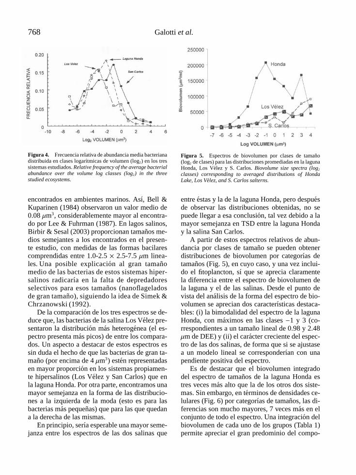
768 Galotti et al.
Figura 4. Frecuencia relativa de abundancia media bacterianadistribuida en clases logarıtmicas de volumen (log2) en los tressistemas estudiados. Relative frequency of the average bacterialabundance over the volume log classes (log2) in the threestudied ecosystems.
encontrados en ambientes marinos. Ası, Bell &Kuparinen (1984) observaron un valor medio de0.08 µm3, considerablemente mayor al encontra-do por Lee & Fuhrman (1987). En lagos salinos,Birbir & Sesal (2003) proporcionan tamanos me-dios semejantes a los encontrados en el presen-te estudio, con medidas de las formas bacilarescomprendidas entre 1.0-2.5 × 2.5-7.5 µm linea-les. Una posible explicacion al gran tamanomedio de las bacterias de estos sistemas hiper-salinos radicarıa en la falta de depredadoresselectivos para esos tamanos (nanoflageladosde gran tamano), siguiendo la idea de Simek &Chrzanowski (1992).
De la comparacion de los tres espectros se de-duce que, las bacterias de la salina Los Velez pre-sentaron la distribucion mas heterogenea (el es-pectro presenta mas picos) de entre los compara-dos. Un aspecto a destacar de estos espectros essin duda el hecho de que las bacterias de gran ta-mano (por encima de 4 µm3) esten representadasen mayor proporcion en los sistemas propiamen-te hipersalinos (Los Velez y San Carlos) que enla laguna Honda. Por otra parte, encontramos unamayor semejanza en la forma de las distribucio-nes a la izquierda de la moda (esto es para lasbacterias mas pequenas) que para las que quedana la derecha de las mismas.
En principio, serıa esperable una mayor seme-janza entre los espectros de las dos salinas que
Figura 5. Espectros de biovolumen por clases de tamano(log2 de clases) para las distribuciones promediadas en la lagunaHonda, Los Velez y S. Carlos. Biovolume size spectra (log2
classes) corresponding to averaged distributions of HondaLake, Los Velez, and S. Carlos salterns.
entre estas y la de la laguna Honda, pero despuesde observar las distribuciones obtenidas, no sepuede llegar a esa conclusion, tal vez debido a lamayor semejanza en TSD entre la laguna Honday la salina San Carlos.
A partir de estos espectros relativos de abun-dancia por clases de tamano se pueden obtenerdistribuciones de biovolumen por categorıas detamanos (Fig. 5), en cuyo caso, y una vez inclui-do el fitoplancton, sı que se aprecia claramentela diferencia entre el espectro de biovolumen dela laguna y el de las salinas. Desde el punto devista del analisis de la forma del espectro de bio-volumen se aprecian dos caracterısticas destaca-bles: (i) la bimodalidad del espectro de la lagunaHonda, con maximos en las clases −1 y 3 (co-rrespondientes a un tamano lineal de 0.98 y 2.48µm de DEE) y (ii) el caracter creciente del espec-tro de las dos salinas, de forma que si se ajustasea un modelo lineal se corresponderıan con unapendiente positiva del espectro.
Es de destacar que el biovolumen integradodel espectro de tamanos de la laguna Honda estres veces mas alto que la de los otros dos siste-mas. Sin embargo, en terminos de densidades ce-lulares (Fig. 6) por categorıas de tamanos, las di-ferencias son mucho mayores, 7 veces mas en elconjunto de todo el espectro. Una integracion delbiovolumen de cada uno de los grupos (Tabla 1)permite apreciar el gran predominio del compo-

Estructura de tamanos en comunidades microbianas salinas 769
Figura 6. Espectro de abundancias de tamanos de las comu-nidades bacterianas y fitoplanctonicas en clases logarıtmicas(log2) para los tres sistemas estudiados. Bacterial and phyto-planktonic size abundance spectrum (log2 classes) in the threestudied ecosystems.
nente fitoplanctonico en la laguna Honda frente ala relativa paridad de los valores de biovolumende la comunidad bacteriana.
El analisis de la forma del espectro dedensidades revela importantes diferencias enla estructura de las comunidades planctonicasanalizadas. Dos son los puntos sobre los que sepuede llamar la atencion: (i) la discontinuidaden la forma del espectro y (ii) el desplazamientoconjunto de las distribuciones de bacteriasy fitoplancton hacia los rangos de mayortamano en las comunidades de las salinas.Este rasgo de la estructura del espectro detamanos, similar al encontrado por Rodrıguezet al. (1990) en la laguna de la Caldera y porHavlicek & Carpenter (2001) para organismosmayores en 11 lagos americanos, parece ser unaconstante de los sistemas acuaticos de interior.No obstante, se aprecia una clara diferenciaentre los sistemas hipersalinos y la lagunasalada. Resulta mucho mas patente el hueco, ladiscontinuidad, del espectro de tamanos en losprimeros como, por otra parte, serıa de esperaren unos ecosistemas de caracter extremo conmenores posibilidades de transferencias demateria y energıa en la red trofica. Se ponede manifiesto que el analisis de espectros detamano puede ser utilizado como un ındice decomplejidad general del ecosistema y relevante
en el diseno de funciones de metas ecologicas(Alvarez-Cobelas & Rojo, 2000).
AGRADECIMIENTOS
Este trabajo ha sido realizado gracias al proyectode investigacion REN2001-3441-CO2-01. Agra-decemos igualmente a la Consejerıa de MedioAmbiente de la Junta de Andalucıa los permisosconcedidos para muestrear en el Paraje Naturalde la laguna Honda.
BIBLIOGRAFIA
AYADI. H., O. ABID, J. ELLOUMI, A. BOUAIN &T. SIME-NGANDO. 2004. Structure of the phyto-plankton communities in two lagoons of differentsalinity in the Sfax saltern (Tunisia). J. PlanktonRes., 26: 69-679.
ALVAREZ-COBELAS, M. & C. ROJO. 2000. Eco-logical goal functions and plankton communitiesin lakes. J. Plankton Res., 22: 729-748.
ANTON, J., R. ROSSELLO-MORA, F. RODRI-GUEZ-VALERA & R. AMANN. 2000. Extremelyhalophylic bacteria in crystallizer ponds from solarsalterns. Applied Environmental Microbiology, 66:3052-3057.
BELL, R. T. & J. KUPARINEN. 1984. Assessingphytoplankton and bacterioplankton produc-tion during early spring in Lake Erken, Swe-den. Applied Environmental Microbiology, 48:1221-1230.
BIRBIR, M. & C. SESAL. 2003. Extremely halophy-lic bacteria communities in Sereflikochisar saltlake in Turkey. Turkey Journal of Biology, 27:7-22.
COLE, J. C., M. L. PACE, N. F. CARACO & G. S.STEINHART. 1993. Bacterial biomass and cellsize distributions in lakes: More and larger cells inanoxic waters. Limnol. Oceanogr., 38: 1627-1632.
CUCCI, T. L. & M. E. SIERACKI. 2001. Effectsof mismatched refractive indices in aquatic flowcytometry. Cytometry, 44: 173-178.
DUSSART, B. 1977. Encyclopedie de l’ecologie, lepresent en question. Larousse, Paris, pp. 66-78.
GAST, V. & K. GOCKE. 1988. Vertical distributionof number, biomass and size-class spectrum ofbacteria in relation to oxic/anoxic conditions in
770 Galotti et al.
the central Baltic Sea. Marine Ecology ProgressSeries, 45: 179-186.
GUERRERO, F. & M. C. CASTRO. 1997. Chlo-rophyll-a of size-fractionated phytoplankton at atemporary hypersaline lake. International Journalof Salt Lake Research, 5: 253-260.
HAMMER, U. T. 1978. The saline lakes of Saskat-chewan. III. Chemical characterization. Int. Revueges. Hydrobiol., 63: 311-335.
HAVLICEK T. D. & S. R. CARPENTER. 2001. Pe-lagic species size distributions in lakes: Are theydiscontinuous? Limnol. Oceanogr., 46: 1021-1033.
JIMENEZ-GOMEZ, F., B. BAUTISTA & V. RODRI-GUEZ. 1994. Trophic interactions in the microbialfood web at a coastal station in the Alboran Sea(Western Mediterranean) in winter. (II). Size selec-tive flagellate feeding on bacteria and its implica-tion on the microbial loop size-structure. ScientiaMarina, 58: 153-159.
LEE, S. & J. A. FUHRMAN. 1987. Relationshipsbetween biovolume and biomass of naturally deri-ved marine bacteriplankton. Applied Environmen-tal Microbiology, 53: 1298-1303.
LI, W. K. W. 1994. Phytoplankton biomass and ch-lorophyll concentration across the North Atlantic.In: The size structure and metabolism of the pela-gic ecosystem. J. Rodrıguez y W. K. W Li (eds.).Scientia Marina, 58 (1-2): 67-79. Barcelona.
MARGALEF, R. 1968. Perspectives in EcologycalTheory. Chicago. University of Chicago Press. 111.
MARGALEF, R. 1983. Limnologıa. Omega. Barce-lona. 1010.
PLATT, T. 1985. Structure of the marine ecosystems:Its allometric basis. In: Ecosystems Theory forBiological Oceanography. R. E. Ulanowicz y T.Platt (eds): Can. Bul. Fish. Aquat. Sci., 213: 55-64.
PLATT, T. 1989. Flow cytometry in Oceanography.In: Cytometry in Aquatic Sciences. C. M. Yentschy P. K. Horan (eds.). Cytometry, 10: 500.
PLATT, T. & K. L. DENMAN. 1978. The structure ofthe pelagic marine ecosystems. Rapp. P.-V. Reun.Cons. Int. Explor. Mer, 173: 60-65.
PORTER K. G. & Y. S. FEIG. 1980. The use of DAPIfor identifying and counting aquatic microflora.Limnol. Oceanogr., 25(5): 943-948.
REUL, A., J. M. VARGAS, F. JIMENEZ-GOMEZ,F. ECHEVARRIA, J. GARCIA-LAFUENTE& J. RODRIGUEZ. 2002. Exchange of plank-tonic biomass through the Strait of Gibraltar in late
summer conditions. Deep-Sea Research II, 49:4131-4144.
RODRIGUEZ, J. & W. K. W. LI (eds.). 1994. The si-ze structure and metabolism of the pelagic ecosys-tem. Scientia Marina, 58 (1-2). 167 pp.
RODRIGUEZ, J., F. ECHEVARRIA & F. JIMENEZ-GOMEZ. 1990. Physiological and ecological sca-lings of body size in an oligotrophic, high moun-tain lake (La Caldera, Sierra Nevada, Spain). J.Plankton Res., 12: 593-599.
RODRIGUEZ, J. & M. M. MULLIN. 1986. Rela-tionship between biomass and body weight ofplankton in a steady state oceanic ecosystem. Lim-nol. Oceanogr., 31: 361-370.
RODRIGUEZ J., J. M. BLANCO, F. JIMENEZ-GOMEZ, F. ECHEVARRIA, J. GIL, V. RODRIGUEZ,J. RUIZ, B. BAUTISTA & F. GUERRERO. 1998.Patterns in the size structure of the phytoplanktoncommunity in the deep fluorescence maximun of theAlboran Sea (southwestern Mediterranean). Deep-SeaResearch I, 45: 1577-1593.
SHELDON, R. W., A. PRAKASH & W. H. SUT-CLIFFE, Jr. 1972. The size distribution of particlesin the ocean. Limnol. Oceanogr., 17: 327-340.
SIERACKI, M. E., P. JOHNSON & J. M. C. N. SIE-BURTH. 1985. Detection, enumeration and sizingof planktonic bacteria by image-analyzed epifluo-rescence microscopy. Applied and EnvironmentalMicrobiology, 49: 799-810.
SIMEK, K. & T. M. CHRZANOWSKI. 1992. Directand indirect evidence of size-selective grazing onpelagic bacteria by freshwater nanoflagellates. Ap-plied Environmental Microbiology, 58: 3715-3720.
SOROKIN, Y. I., 1999. Aquatic Microbial Ecology:a text book for students in environmental sciences.Leiden. Backhuys Publishers. 248 pp.
SPRULES, W. G. 1988. Effects of trophic interac-tions on the shape of pelagic size spectra. Verh.Internat. Verein. Limnol. 23: 234-240.
UNESCO. 1994. Protocols for the Joint Global OceanFlux Study (JGOFS) Core Measurements. SCOR–IOC–UNESCOManuals andGuides. 29. 178pp.
WETZEL, R. G. & M. SONDERGAARD. 1998. Ro-le of submerged macrophytes for the microbialcommunity and dynamics of dissolved organic car-bon in aquatic ecosystems. In: The structuring roleof submerged macrophytes in lakes. E. Jeppesen,M. Sondergaard y K. Christoffersen (eds.): 133-148. Springer-Verlag, Nueva York.

Limnetica, 25 (3-4): xx-xx (2006)Limnetica, 25 (3): 771-786 (2006)c© Asociacion Espanola de Limnologıa, Madrid. Spain. ISSN: 0213-8409
Spatial and temporal heterogeneity in the Alqueva reservoir, Guadianariver, PortugalA
Antonio Serafim1,∗, Manuela Morais1, Pedro Guilherme1, Paula Sarmento2, Manuela Ruivo2,Ana Magrico2
1 Water Laboratory, Environment and Ecology Center, University of Evora, Rua da Barba Rala, no 1, P.I.T.E.,7005-345 Evora, Portugal.2 EDIA-Empresa de Desenvolvimento e Infra-Estruturas do Alqueva, S.A; Rua Zeca Afonso, no 2; 7800-522Beja, Portugal.2 EDIA∗ Corresponding author: [email protected]
ABSTRACT
Spatial and temporal heterogeneity in the Alqueva reservoir, Guadiana river, Portugal
This study aims to assess the physico-chemical variability of the Alqueva reservoir during its initial filling period. The datasetconsists of analytical results from an 11 month survey (Mar 2003-Jan 2004) conducted in the water body, at three levels ofdepth in the several tributaries and in the discharge section. 21 parameters were monitored on a monthly base, in order tounderstand the temporal and spatial variability. Another goal of this work was to use a multivariate statistical approach to helpunderstand the relationships between water quality parameters, to group zones according to their similarities and to distinguishbetween wet and dry season conditions. FA/PCA needs 6 VF/PC to point out 74 % in the wet season, and 7 VF/PC to explain78.6 % of variance in the dry season. FA/PCA allows grouping the selected parameters according to common features. As aresult, mineral content is indicated as the principal source of variability in the wet season, while oxygenation plays the mainrole in the dry season. DA renders an important data reduction using 10 parameters to provide 93.2 % right assignations duringtemporal analysis. DA assigns temporal variability to the consequences of water balance on ambient salinities, to stratificationinfluences and to surface runoff. Also, it uses only 4 parameters to yield 71.3 % right assignations during the spatial analysisin the dry season. Conductivity declines in the lacustrine zone, while CBO5, pH and Temperature vary principally in thevertical sense. However, such a spatial pattern is not static. It can become either more defined during the dry season, orless evident during the expansion of the lotic conditions in the rainy period (late spring and summer). Seasonal processesof stratification/mixture determine the temporal changes in the lacustrine zone. The system seems to be affected by periodicpulses of modifications produced by intensive rains and drought. Thus, limnological understanding of these questions is aprerequisite for making wise judgments about reservoir management.
Key words: Alqueva reservoir, water quality, dry season, wet season, principal component analysis, factor analysis,discriminant analysis.
RESUMEN
Heterogeneidad espacial y temporal en el embalse de Alqueva, rıo Guadiana, Portugal
Este estudio apunta a determinar la variabilidad fisco-quımica del embalse de Alqueva en su perıodo de llenado inicial. Elconjunto de datos consiste en resultados analıticos a partir de los primeros once meses de muestreo (marzo de 2003-enero de2004) conducida en el cuerpo del agua, en tres niveles de profundidad; en los varios tributarios y en la seccion de la descarga.21 parametros se han supervisado en una base mensual, para entender la variabilidad temporal y espacial. Otra meta de estetrabajo fue el utilizar un acercamiento estadıstico multivariado para ayudar a entender las relaciones entre los parametrosde la calidad del agua; para agrupar zonas segun sus semejanzas y distinguir entre las condiciones de las estaciones humeday seca. FA/PCA necesita 6 VF/PC para precisar 74 % de la estacion humeda, y 7 VF/PC para explicar 78.6 % de la variacionen la estacion seca. FA/PCA permite agrupar los parametros seleccionados segun caracterısticas comunes. Como resultadoel contenido mineral se senala como la fuente principal de la variabilidad en la estacion humeda, mientras que la oxigenaciondesempena el papel principal en la estacion seca. DA rinde una reduccion de datos importante usando 10 parametros paraproducir 93.2 % de clasificaciones correctas durante analisis temporal. DA asigna variabilidad temporal a las consecuencias

772 Serafim et al.
del balance del agua en salinidades, a las influencias de la estratificacion y a la salida superficial. Ademas, utiliza solamente4 parametros para rendir 71.3 % clasificaciones correctas durante el analisis espacial en la estacion seca. La conductividaddecae en la zona lacustre, mientras que CBO5, el pH y la temperatura varıan principalmente en el sentido vertical. Sinembargo, un patron tan espacial no es estatico. Puede hacerse mas definido durante la estacion seca, o menos evidentedurante la expansion de las condiciones loticas en el perıodo lluvioso (fin de primavera y verano). Los procesos estacionalesde la mezcla de la estratificacion determinan los cambios temporales en la zona lacustre. El sistema parece afectado porpulsos periodicos de las modificaciones producidas por las lluvias intensivas y sequıa. Ası la comprension limnologica deestas preguntas es un requisito previo para hacer juicios sabios sobre la gerencia del embalse.
Palabras clave: Embalse de Alqueva, calidad del agua, estacion seca, estacion humeda, analisis de componentes principales,analisis factorial, analisis discriminante.
INTRODUCTION
As well as creating a new water resource, theconstruction of a dam may also involve substan-tial modifications to the environment, during bothconstruction and subsequent operation (Crouzet& Leonard, 1999; Bergkamp et al., 2000). Thesechanges include increases in residence time, tem-perature, stratification, and reduction in turbu-lence, most often a decrease in particles and tur-bidity, and sometimes an increase oinautochtho-nous primary production (Friedl & Wuest, 2002).The variability and complexity of these changesis reflected in the water quality. If water qualitydeteriorates in a reservoir, it may become unsui-table for its original purposes and costly mea-sures may be required to combat the problem.It also constitutes a threat to the downstreamecosystem (Ferreira, 1999). The water quality ofreservoirs is controlled by several factors, amongwhich the interaction of the lacustrine end withthe catchment area plays an important role (Car-penter & Cottingham, 1997; Wetzel, 1993). Thisfeature assumes particular importance in newlyflooded areas. Thus, the success of reservoir ma-nagement and restoration projects depends on thedetection of spatial and temporal changes in re-servoir status that reflect changes in the surroun-ding environment. Seasonal climate changes arethe most relevant, particularly rainfall and solarheating, resulting in seasonal variations in waterquality (Chapman, 1996). The assessment of longterm trends (seasonal, annual) is related directlyto the reservoir management strategies requiredto understand the processes occurring within the
reservoir and to provide more detailed informa-tion on a variety of indicators of reservoir con-dition (Hoyos & Comın, 1999). This seasonalmonitoring assumes particular importance in thePortuguese southern semi-arid areas, where theriver discharge may range from zero in the dryseason to high discharge rates during the rainyseason (Morais, 1995; Bernardo & Alves, 1999).Subjected to a great variability of the hydrolo-gic regime, tributaries experiment wide rangesin physical-chemical and biological parameters(Morais, 1995), affecting the reservoirs down-stream. Therefore, the understanding of variousphenomena relating to the characteristics of thereservoir and its catchment area is the most ba-sic step in evaluating water quality and judgingspecific problems (Hwang et al., 2003).
The chemistry of standing waters is intima-tely linked to the physical processes occurringwithin the water body as well as in the atmos-phere and the catchment. Physical features withhigh seasonal variation such as light and tempera-ture play key roles in most chemical transforma-tions, either by accelerating chemical or enzymicreactions or by promoting photosynthesis (Boul-ton & Brock, 1999). When changing a stretchof a river to a reservoir, the slowdown of theflow subsequently evokes particle settling, tur-bidity decreases and light transmissivity increa-ses, enhancing in situ primary production. Thus,from the headwater of the reservoir to the dam theriver changes from an allochthonous-dominatedsystem to a more lacustrine system, where auto-chthonous production of organic matter domina-tes (Friedl & Wuest, 2002). Therefore, the exis-

Spatial and temporal heterogeneity in the Alqueva reservoir 773
tence of progressive physical, chemical and bio-logical changes along the main axis of the re-servoir frequently reflect strong spatial gradients.Seasonal events can make the spatial structureeven more complex, both vertically and hori-zontally (Catalan & Fee, 1994; Wetzel, 1993).Due to those spatial and temporal variations, amonitoring programme that will provide a re-presentative and reliable estimation of the qua-lity of reservoir water is necessary (Simeonovet al., 2003). The usual situation is the measu-rement of multiple parameters, taken at diffe-rent monitoring times and from many monito-ring stations. Therefore, a complex data matrixis frequently needed to evaluate water quality(Chapman, 1996). Furthermore, it is a commonexperience to face the problem of determiningwhether a variation in the concentration of mea-sured parameters should be attributed to pollution(man-made, spatial) or to natural (temporal, cli-matic) changes. Also, it is necessary to determinewhich parameters are the most significant fordescribing such spatial and temporal variations,the sources of pollution, etc. Therefore, the useof multivariate techniques has increased in recentyears, mainly due to the need to obtain appre-ciable data reduction for analysis and decision-making (Chapman, 1996, Vega et al., 1998,Pesce & Wunderlin, 2000, Helena et al., 2000).
In this context, this study aims to assessphysical-chemical seasonal variability of the Al-queva reservoir (Guadiana river basin). Knowingthat reservoirs formed by river impoundmentundergo great changes in water quality duringthe early stages of their formation whilst anew ecological balance is becoming established,EDIA (Empresa de Desenvolvimento e Infra-Estruturas de Alqueva), with the beginning ofthe filling phase (February 2002), implementeda monitoring programme that provides anevaluation of spatial and temporal variationsin water chemistry and biology. This paperdocuments water quality in the features of inputflux, state and discharge, during 11 months inthe filling phase. Another goal of this work is touse a multivariate statistical approach to aid theunderstanding of the relationships between waterquality parameters, to group zones according to
Table 1. Land use in the Portuguese side of the catchmentarea using CORINE land cover classes. Usos de la tierra en ellado portugues de la cuenca utilizando las clases de coberturaCORINE.
Classes % ocupation
Artificial Areas 0.75Agriculture 69.83Semi-natural 28.50Aquatic Areas 0.89No information 0.03Total 100
their similarities and to distinguish between wetand dry season conditions.
STUDY AREA
The Alqueva reservoir, located in southern Portu-gal along 83 km of the main course of the Gua-diana river, constitutes the biggest artificial lakeon the Iberian Peninsula. It can store 4500 hm3 ofwater, with a dentiform surface of 25000 ha. Thecatchment area is 55 000 km2. The Portugueseside covers only 4310 km2.
During the study period, the climate on thePortuguese side of the catchment area was cha-racterized by a mean temperature of 17.5 ◦C ran-ging from 4.5 ◦C in January to 33.3 ◦C in Au-gust. The total precipitation was 358mm, and thepotential evapotranspiration 271mm. The annualinsulation is 2859 h. The dry season extends fromMay to September. The bed rocks are dominatedby granite and gneiss mainly covered by Aluvis-solos and Litossolos. The Land use in the Portu-guese side of the catchment is presented in Table1, and it was calculated using CORINE land co-ver classes. Notice that 69.8 of the catchment isused for agriculture, while the semi-natural areasonly represent 28.5 %.
METHODOLOGY
Sampling and analytical procedures
In total, 8 collection sites were established, 4 withlentic characteristics sampled at 3 levels of depth(surface, middle and bottom) and 4 with lotic

774 Serafim et al.
Figure 1. Map of the reservoir and sampling site locations. Mapa del embalse y situacion de las estaciones de muestreo.
characteristics sampled from the margin (Fig. 1).The sites Sr.a da Ajuda (SA), Alcarrache (Alc)and Alamos (Ala), provide a monitorization ofthe input flux. Albufeira Mourao (Mou) and Al-
queva Montante (AM), located in the water body,provide the state monitoring, while Alqueva Ju-sante (AJ) provides the outlet monitoring. Thesites Ardila (Ard) and Moinho das Barcas (MB)

Spatial and temporal heterogeneity in the Alqueva reservoir 775
are useful in evaluating the water quality in thedownstream ecosystem. They also aid in esta-blishing a reference of water quality prior to theconstruction of the Pedrogao Reservoir, whichwill be located immediately downstream fromthe Alqueva Dam. Monthly monitoring was donefrom March 2003 to January 2004. Vertical pro-files were made of Temperature, Dissolved Oxy-gen, pH and Conductivity, in sites located in thewater body, using a 3L Van Dorn bottle to co-llect water samples, and a WTW 350i probe,with a pH electrode WTW pH Sentix 41-3 anda combined Conductivity –Oxygen probe WTWConOx– 3 to conduct the measurements. Sam-ples for analysis were collected at the surface,the middle and the bottom. At sites locatedin water streams, measurements and samplingwhere done from the bank. In the laboratory,16 parameters were determined by using officialrecommended methods of analysis (A.P.H.A.,1998). Measured parameters include: Nitrate(4500-NO−3 E.); Ammonium (4500-NH3 F.); To-tal Nitrogen (TN) [Kjeldahl nitrogen (4500-Norg) + nitrates); Soluble Reactive Phosphorus(SRP) (4500-P E.); Total Phosphorus (TP) (4500-P E., after acid digestion); 5-day BiologicalOxygen Demand (BOD-5) (5210 B.); Chemi-cal Oxygen Demand (COD) (5220 C); Per-manganate Oxidizable Compounds (POC) (Ro-dier, 1981); Magnesium (Hardness-Calcium);Calcium (3500-Ca D); Chloride (4500-Cl− B.);Hardness (2340 C.); Alkalinity (2320-B); To-tal Dissolved Solids (TDS) (2540-C) and TotalSuspended Solids (2500 D.-TSS).
Statistical treatment of data
Statistical analysis was applied on experimentaldata normalized to zero mean and unit variance(standardized data) in order to avoid misclassifi-cations arising from the different orders of mag-nitude. We studied the correlation structure bet-ween variables using the Pearson coefficient. Themultivariate approach was performed using twotechniques: factor analysis (FA), including prin-cipal component analysis (PCA) and discrimi-nant analysis (DA). Principal component analysis(PCA) allowed ending out associations between
variables, thus reducing the dimensionality of thedata table. This is accomplished by diagonaliza-tion of the correlation matrix of the data, whichtransforms the 19 original variables into 19 unco-rrelated (orthogonal) ones (weighed linear com-binations of the original variables) called prin-cipal components (PCs). The eigenvalues of thePCs are a measure of their associated variance,the participation of the original variables in thePCs is given by the loadings, and the individualtransformed observations are called scores (John-son and Wichern, 1992; Reis, 1998; Vega et al.,1998; Helena et al., 2000; Pesce & Wunderlin,2000). In practice, FA follows PCA. The mainpurpose of FA is to reduce the contribution ofless significant variables in order to simplify evenmore of the data structure coming from PCA, atthe cost of a loss of orthogonality. This last pur-pose was achieved by performing a Varimax ro-tation in the axis defined by PCA. Discriminantanalysis (DA) provides statistical classification ofsamples. We can use DA if we know in advancethe membership of objects to particular groups orclusters (i.e., the temporal or spatial ownershipof a water sample as determined from its monito-ring time or station). We can construct a discrimi-nant function for each group; this function has theform presented in Johnson and Wichern (1992). Itrepresents a surface dividing our data space intoregions; then samples sharing common propertieswill be grouped into the same region with a de-cision boundary separating two or more groups.The efficiency of these discriminant functionscan then be checked with the same data set usingthe cross validation method (Miller & Miller,2000). DA was performed on each data matrixby using the standard and the stepwise modes.The best discriminant function for each situa-tion was selected considering the goodness of theclassification matrix and the number of parame-ters needed to reach such a matrix. The statisti-cal package SPSS 11.5 was used for calculation.
RESULTS AND DISCUSSION
Our first approach to establish the parametersassociated with temporal variation was using

776 Serafim et al.
Figure 2. Temperature profiles at Alqueva Montante from March 2003 (1) to January 2004 (11). Perfiles de temperatura de AlquevaMontante desde Marzo de 2003 (1) a Enero de 2004 (11).
the Pearson correlation coefficient. To perform aPearson evaluation, each season was transformedinto a numerical value in the data matrix (Wet =1 and Dry = 2); this numerical variable was thencorrelated (pair by pair) with all the measured pa-rameters. The results show that the water tempe-rature exhibits the highest correlation coefficient(r = 0.551; p < 0,01; n = 176) with the season.In addition to the temperature, we observed sevenadditional parameters having significant correla-tion with the season ( p < 0.01): TDS (r = 0.536),Alkalinity (r = 0.398), TP (r = −0.307), Con-ductivity (r = 0.287), Calcium (r = 0.279), Mag-nesium (r = 0.213), and SRP (r = −0.195). Sofar, this group could be taken as representing themajor source of temporal changes in water qua-lity. Many of these correlations can be explainedin view of the climatic features associated withthe wet season (October to April) and dry season(May to September). So it is evident that the wa-ter temperature reflects the atmospheric tempe-rature, and that this parameter presents the mostsignificant difference between both seasons. Thetemperature data demonstrate that the reservoiris stratified from May to September, the dry sea-son. The water temperature profiles in AlquevaMontante are shown in figure 2. In autumn andwinter, all the study locations exhibit isothermalprofiles of temperature. Seasonal climate chan-
ges, particularly rainfall and solar heating, resultin seasonal variations in water balance producinga predictable variation in water level. In the dryseason, the water balance is maintained by eva-poration. This leads to an increase in salt content,reflected by higher levels of Total Dissolved So-lids, Alkalinity, Calcium and Magnesium. Des-pite this slight increase, water uses were not com-promised. As reported by Lory (1995), higher le-vels of TP and SRP in the wet season reflect therunoff from the catchment area, especially duringflood events. In the dry season, nutrient uptakeby phytoplankton can deplete Soluble ReactivePhosphorus (Selig et al., 2002), justifying the lo-wer concentrations observed.
Looking for more evidence on both patternsand parameters associated with the temporal va-riation, we carried out PCA. Tables 2 and 3 sum-marize the PCA results, including the loadings(participation of the original variables in the newones). PCA for the wet season renders 6 PrincipalComponents (PC) with eigenvalues higher than1, accounting for 74 % of total variance. PC1 ex-plains 24 % of the variance, and is contributedby Conductivity, Calcium, Chloride, Magnesium,TDS, Hardness and Alkalinity. Thus, PC1 repre-sents the parameters associated with dissolvedsalts responsible for mineralization. PC2 explains15 % of the total variance, with Dissolved Oxy-

Spatial and temporal heterogeneity in the Alqueva reservoir 777
Table 2. Loadings of 21 experimental variables on six significant principal components for the wet season. Pesos de 21 variablesexperimentales para los 6 componentes principales significativos para la estacion humeda.
Variable PC 1 PC 2 PC 3 PC 4 PC 5 PC 6
DO mg/L −0.504 0.748 0.143 −0.105 0.312 0.055DO % sat −0.501 0.720 0.171 −0.062 0.330 0.076pH −0.483 0.747 0.068 −0.049 0.148 0.046T 0.097 0.252 0.663 0.218 −0.240 0.120Conductivity 0.848 0.253 −0.032 0.138 −0.065 0.026NO3 −0.294 0.350 –0.558 0.587 −0.082 0.016TN −0.309 0.345 –0.576 0.580 −0.076 0.010NH4 0.207 –0.459 0.296 0.325 0.493 0.315SRP 0.107 −0.174 0.029 0.295 0.685 0.482TP −0.123 −0.256 −0.027 −0.349 0.533 −0.294COD 0.345 −0.034 0.640 0.235 −0.345 0.160BOD −0.046 0.250 0.689 0.256 0.044 −0.158TOC −0.279 –0.317 –0.359 0.305 −0.217 0.205POC −0.210 −0.277 0.350 0.622 0.135 −0.277Ca 0.741 0.418 −0.018 0.045 −0.005 0.125Cl 0.634 0.264 −0.221 0.147 −0.090 −0.088Mg 0.471 −0.168 −0.325 0.083 0.406 −0.002TDS 0.836 0.338 −0.047 −0.031 0.022 −0.038TSS 0.158 −0.023 0.092 0.385 0.255 –0.719Hardness 0.795 0.283 −0.179 −0.134 0.223 −0.117Alkalinity 0.788 0.160 0.003 0.021 0.048 0.062Eigenvalue 5.109 3.045 2.561 1.879 1.776 1.173% Variance explained 24.32 14.50 12.19 8.94 8.45 5.58% Cum. variance 24.32 38.82 51.02 59.96 68.42 74.00
gen and pH the main participants. PC3 (12.2 %of the variance) represents principally Tempera-ture, BOD, COD and also Nitrate, TN, and TOC.PC4 is highly contributed by POC, Nitrate andTotal Nitrogen. PCs 3 and 4 can, then, be relatedto the input of dissolved and particulate organicmatter. PC5 is mainly related to nutrients, whilePC6 represents the TSS. The bivariate plot of theloadings of PCs 1 and 2 (Fig. 3) shows that thesamples corresponding to the Alamos, Alcarra-che, Ardila and Barcas locations appear on thepositive side of PC1, due to its higher minerali-zation. In the negative side, in the third quadrant,appear the samples collect in October, mainly dueto high concentrations of TOC, POC and TP. Thehigher levels of precipitation that occurred mayhave resulted in the surface runoff of phosphorusand organic compounds from the catchment area,justifying this individualization.
In the dry season, seven principal components
were obtained with eigenvalues > 1, making up78.6 % of total variance in the dataset; these areshown in Table 3. The first PC accounting for18.3 % of total variance is correlated primarilywith Dissolved Oxygen and pH and secondarilywith Temperature, organic variables and SRP,although this last is negatively correlated with therest. The second PC accounting for 15.14 % ofthe total variance is correlated with Conductivity,Hardness, TDS and Calcium. The scatter plotof PCs 1 and 2 for the samples shows that allthe situations of middle and bottom are locatedon the positive side of PC1, principally due tothe consequences of stratification. In the dryseason, surface layers heat up and form a warmlayer (epilımnion) overlying cooler, denser water(hipolımnion). In Alqueva Montante (the deepestsite), the amplitude between surface and bottomTemperature reached 17 ◦C. This stratificationprevents water mixing and results in the depletion

778 Serafim et al.
Table 3. Loadings of 21 experimental variables on seven significant principal components for the dry season. Pesos de 21 variablesexperimentales para los siete componentes principales significativos para la estacion seca.
Variable PC 1 PC 2 PC 3 PC 4 PC 5 PC 6 PC 7
DO mg/L 0.747 −0.050 0.383 −0.162 0.181 0.393 0.026DO % sat 0.688 −0.277 0.393 −0.177 0.206 0.356 0.011pH 0.855 0.023 0.305 −0.016 −0.057 0.050 −0.011T 0.638 −0.235 −0.013 −0.152 0.138 −0.326 0.320Conductivity −0.110 0.748 0.349 −0.235 −0.087 −0.239 0.048NO3 −0.079 0.081 0.656 0.663 0.096 −0.154 0.059TN −0.020 0.081 0.602 0.720 0.081 −0.116 0.063NH4 −0.345 0.221 –0.463 0.304 0.430 0.064 0.114SRP –0.388 0.361 0.264 0.341 0.283 0.116 −0.054TP −0.016 −0.223 −0.223 0.331 0.048 0.117 0.654COD 0.599 0.316 –0.497 0.204 −0.040 −0.029 −0.165BOD 0.629 0.510 −0.122 0.254 −0.034 −0.184 −0.059TOC 0.445 0.017 0.017 0.515 −0.171 0.186 −0.168POC 0.470 0.132 –0.561 0.207 0.024 −0.225 0.389Ca −0.031 0.662 0.267 −0.413 0.337 −0.139 0.252Cl 0.224 0.485 0.051 −0.190 –0.557 −0.150 0.119Mg −0.185 0.247 −0.224 0.223 –0.619 0.509 0.121TDS −0.013 0.606 0.117 −0.121 0.052 −0.033 −0.155TSS 0.333 0.392 –0.505 0.262 0.171 −0.047 −0.364Hardness −0.115 0.675 0.145 −0.063 −0.215 0.388 0.269Alkalinity −0.014 0.393 −0.286 −0.131 0.610 0.398 0.023Eigenvalue 3.840 3.180 2.715 2.187 1.678 1.294 1.088% Variance explained 18.28 15.14 12.92 10.41 7.99 5.94 5.18% Cum. variance 18.28 33.42 46.35 56.76 64.76 70.71 75.88
Figure 3. Distribution of the water samples from the wet season on the plane defined by the first two principal components.Distribucion de las muestras de la estacion humeda en el plano definido por los dos primeros componentes principales.

Spatial and temporal heterogeneity in the Alqueva reservoir 779
Table 4. Loadings of 21 experimental variables on six significant varifactors for the wet season. Pesos de 21 variablesexperimentales para 6 seis varifactores significativos para la estacion humeda.
Variable VF 1 VF 2 VF 3 VF 4 VF 5 VF 6
DO mg/L −0.133 0.960 0.054 0.011 −0.042 −0.028DO % sat −0.145 0.944 0.061 0.040 0.009 −0.012pH −0.113 0.868 0.170 0.049 −0.149 −0.059T 0.074 0.158 −0.110 0.767 −0.002 0.049Conductivity 0.863 −0.169 0.017 0.180 0.033 0.009NO3 −0.016 0.202 0.896 −0.127 −0.047 0.090TN −0.028 0.204 0.901 −0.151 −0.052 0.090NH4 −0.023 −0.235 −0.155 0.140 0.819 0.136SRP 0.061 0.076 0.040 −0.087 0.901 −0.030TP −0.178 0.075 –0.435 −0.511 0.152 0.249COD 0.168 −0.214 −0.170 0.790 0.058 0.011BOD −0.030 0.312 −0.177 0.596 0.055 0.380TOC −0.339 −0.320 0.487 −0.084 0.076 −0.146POC −0.329 −0.121 0.150 0.314 0.275 0.637Ca 0.836 0.047 0.004 0.166 0.036 −0.106Cl 0.709 −0.125 0.167 0.009 −0.092 0.056Mg 0.428 −0.222 0.011 −0.381 0.369 0.113TDS 0.895 −0.046 −0.102 0.063 −0.028 0.001TSS 0.159 −0.042 0.016 −0.050 −0.022 0.857Hardness 0.869 −0.009 −0.163 −0.197 0.029 0.054Alkalinity 0.770 −0.155 −0.116 0.099 0.114 −0.027Eigenvalue 4.650 3.12 2.27 2.26 1.78 1.44% Variance explained 22.14 14.87 10.84 10.78 8.49 6.86% Cum. variance 22.14 37.02 47.86 58.64 67.14 74.00
of hypolimnetic oxygen due to the mineralizationof organic matter settled on the bottom (Chap-man, 1996). In figure 4, it can be seen that, du-ring the stratified period, the hipolımnion is un-der anoxic conditions. Notice that, when stratifi-cation is disrupted (September-October), the cir-culation of water tends to mix anoxic water formthe bottom through all the vertical profile, lowe-ring surface concentrations of Dissolved Oxygen.This can seriously compromise water uses. Con-trary to Boulton & Brock (1999), this period wasnot followed by an extensive growth of phyto-plankton. This is understandable since the pro-cesses of internal loading are not expressive dueto the youth of the reservoir.
Surface situations in the reservoir and wa-ter courses appear on the negative side of PC1,mainly related to low levels of SRP and Ammo-nia, indicating high levels of nutrient uptake byphytoplankton (Fig. 5). Third and fourth PCs re-
present the importance of nutrients in total varia-bility (12.9 % and 10.4 % of variance). PCs 5, 6and 7 explain less than 10 % of variance each.
The values of PCA can be clarified by meansof a Varimax rotation of the eigenvalues. Bythis method, varivalues and varifactors (VFs)are obtained, in which original variables parti-cipate more clearly. Table 4 shows the 6 VFsfor the wet season spanning the same 74 %of variance. The amount of information ex-plained by VF1 (22.1 %) is very similar toPC1 (24.3 %), with participation also by Con-ductivity, Calcium, Chloride, Magnesium, TDS,Hardness and Alkalinity. VF2 (14.9 % of va-riance) accounts for Dissolved Oxygen and pH.VFs 3, 4 and 5 explain the importance of nu-trients in the variability of water quality du-ring the wet period (10.8 %, 10.8 % and 8.5 %).These “nutrient” factors represent influencesfrom non-point sources such as agricultural

780 Serafim et al.
Figure 4. Dissolved Oxygen (% saturation) profile at Alqueva Montante from March 2003 (1) to January 2004 (11). Oxıgenodisuelto (% de saturacion) en Alqueva Montante desde Marzo de 2003 (1) a Enero de 2004 (11).
Table 5. Loadings of 21 experimental variables on seven significant varifactors for the dry season. Pesos de 21 variablesexperimentales para los siete varifactores para la estacion seca.
Variable VF 1 VF 2 VF 3 VF 4 VF 5 VF 6 VF 7
DO mg/L 0.953 0.086 0.045 0.012 0.057 −0.021 −0.012DO % sat 0.934 −0.041 −0.126 −0.006 0.022 −0.121 −0.011pH 0.782 0.351 0.078 0.079 −0.272 −0.087 0.032T 0.428 0.191 −0.007 −0.154 −0.242 –0.474 0.432Conductivity −0.097 0.009 0.863 0.136 −0.110 0.045 −0.167NO3 0.038 −0.071 0.052 0.949 −0.084 −0.047 0.014TN 0.061 0.004 0.006 0.949 −0.072 −0.005 0.047NH4 −0.458 0.172 −0.033 0.065 0.621 0.013 0.215SRP −0.206 −0.095 0.224 0.522 0.392 0.117 −0.149TP −0.050 −0.069 −0.243 0.103 0.124 0.140 0.735COD 0.121 0.851 −0.011 −0.168 0.034 0.059 0.070BOD 0.211 0.781 0.294 0.132 −0.092 −0.011 0.082TOC 0.284 0.475 −0.272 0.322 −0.100 0.247 −0.021POC −0.023 0.612 −0.006 −0.175 −0.010 −0.087 0.621Ca 0.081 −0.096 0.877 −0.019 0.243 −0.180 0.039Cl 0.030 0.242 0.521 −0.139 −0.482 0.297 0.033Mg −0.170 0.082 −0.039 −0.050 −0.079 0.895 0.079TDS −0.034 0.181 0.549 0.053 0.117 0.071 −0.258TSS −0.094 0.803 −0.002 −0.069 0.270 −0.023 −0.139Hardness 0.049 −0.026 0.598 0.060 0.139 0.612 0.062Alkalinity 0.087 0.142 0.234 −0.189 0.816 0.032 0.011Eigenvalue 3.041 2.925 2.799 2.385 1.804 1.659 1.322% Variance explained 14.48 13.93 13.32 11.35 8.59 7.90 6.29% Cum. variance 14.48 28.41 41.74 53.10 61.69 69.59 75.89
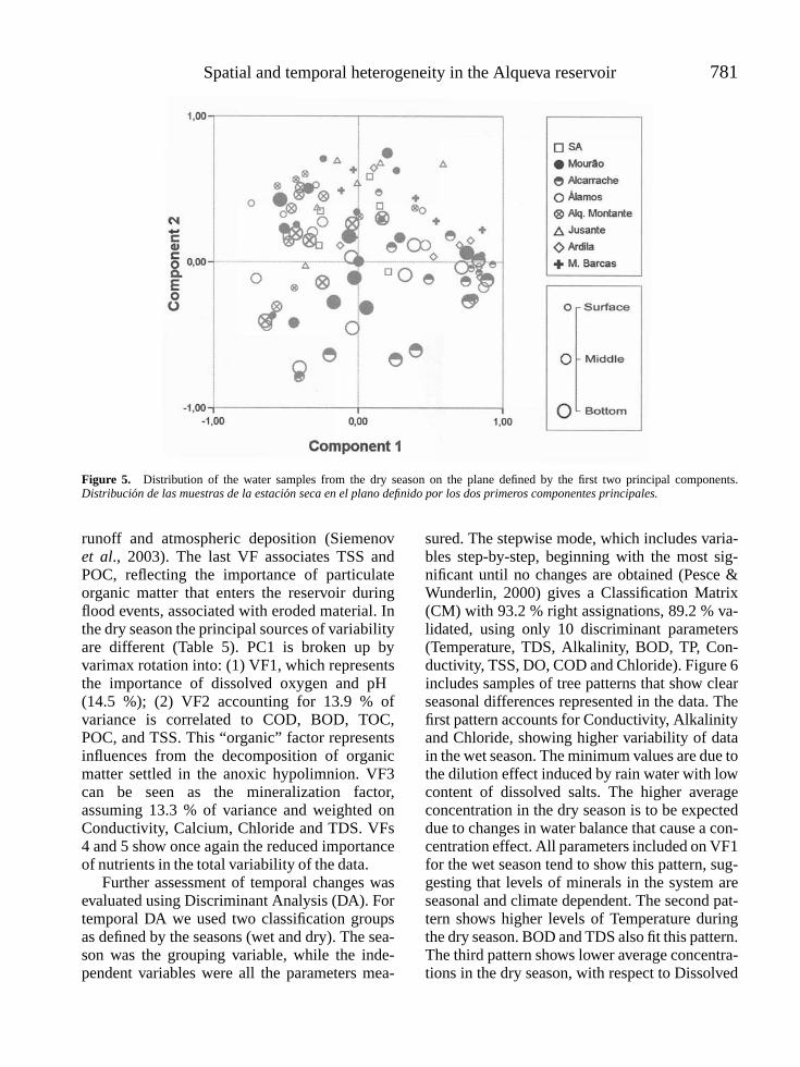
Spatial and temporal heterogeneity in the Alqueva reservoir 781
Figure 5. Distribution of the water samples from the dry season on the plane defined by the first two principal components.Distribucion de las muestras de la estacion seca en el plano definido por los dos primeros componentes principales.
runoff and atmospheric deposition (Siemenovet al., 2003). The last VF associates TSS andPOC, reflecting the importance of particulateorganic matter that enters the reservoir duringflood events, associated with eroded material. Inthe dry season the principal sources of variabilityare different (Table 5). PC1 is broken up byvarimax rotation into: (1) VF1, which representsthe importance of dissolved oxygen and pH(14.5 %); (2) VF2 accounting for 13.9 % ofvariance is correlated to COD, BOD, TOC,POC, and TSS. This “organic” factor representsinfluences from the decomposition of organicmatter settled in the anoxic hypolimnion. VF3can be seen as the mineralization factor,assuming 13.3 % of variance and weighted onConductivity, Calcium, Chloride and TDS. VFs4 and 5 show once again the reduced importanceof nutrients in the total variability of the data.
Further assessment of temporal changes wasevaluated using Discriminant Analysis (DA). Fortemporal DA we used two classification groupsas defined by the seasons (wet and dry). The sea-son was the grouping variable, while the inde-pendent variables were all the parameters mea-
sured. The stepwise mode, which includes varia-bles step-by-step, beginning with the most sig-nificant until no changes are obtained (Pesce &Wunderlin, 2000) gives a Classification Matrix(CM) with 93.2 % right assignations, 89.2 % va-lidated, using only 10 discriminant parameters(Temperature, TDS, Alkalinity, BOD, TP, Con-ductivity, TSS, DO, COD and Chloride). Figure 6includes samples of tree patterns that show clearseasonal differences represented in the data. Thefirst pattern accounts for Conductivity, Alkalinityand Chloride, showing higher variability of datain the wet season. The minimum values are due tothe dilution effect induced by rain water with lowcontent of dissolved salts. The higher averageconcentration in the dry season is to be expecteddue to changes in water balance that cause a con-centration effect. All parameters included on VF1for the wet season tend to show this pattern, sug-gesting that levels of minerals in the system areseasonal and climate dependent. The second pat-tern shows higher levels of Temperature duringthe dry season. BOD and TDS also fit this pattern.The third pattern shows lower average concentra-tions in the dry season, with respect to Dissolved

782 Serafim et al.
Figure 6. Patterns observed with temporal variations: (A) dilution (observed during the wet season); (B) Seasonal differences; (C)TP increase (observed during the wet season) and DO decrease, observed during the dry season. Patrones de variacion temporalobservados: (A) dilucion observada durante la estacion humeda; (B) Diferencias estacionales; (C) Incremento del TP observadodurante la estacion seca y disminucion del OD, observado durante la estacion seca.
Oxygen and TP. These last two patterns are con-nected, taking into account that high levels of or-ganic matter (BOD) consume large amounts ofoxygen. The decrease of TP during the dry sea-son is expectable due to the reduced presence oferoded material abundant only in flood events.
We carried out spatial DA for both seasonsas the next step. An additional problem inspatial DA is to define the number of groups,where each group accounts for a studied area.We found that the best results (in terms ofpercentage of right assignations from the DF)are obtained when grouping middle and bottomsituations. The DA stepwise mode classificationmatrix for the wet season shows 40.6 % rightassignations and only 33.3 % validated, selecting
3 parameters responsible for spatial variations:Dissolved Oxygen, Temperature and Calcium.The low differentiation between areas is expec-ted due to the homogeneity of the water mass,with the expansion of lotic condition in the rainyperiod (Nogueira, et al., 1999). DA results forthe dry season show that only 4 parameters areenough to obtain a good differentiation betweenthe 12 areas (71.3 % right classifications): pH,Temperature, Conductivity and BOD. Figure 7includes 2 patterns represented in the spatialanalysis of the data. The first pattern accountsfor high values for BOD, pH and Conductivityupstream in Sra da Ajuda (1), near theborder with Spain, often associated with certaineffluents (Chapman, 1996). We can observe a
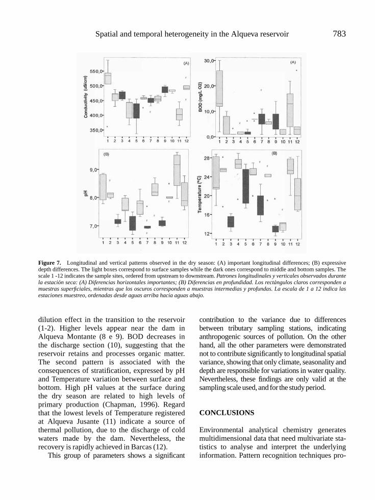
Spatial and temporal heterogeneity in the Alqueva reservoir 783
Figure 7. Longitudinal and vertical patterns observed in the dry season: (A) important longitudinal differences; (B) expressivedepth differences. The light boxes correspond to surface samples while the dark ones correspond to middle and bottom samples. Thescale 1 -12 indicates the sample sites, ordered from upstream to downstream. Patrones longitudinales y verticales observados durantela estacion seca: (A) Diferencias horizontales importantes; (B) Diferencias en profundidad. Los rectangulos claros corresponden amuestras superficiales, mientras que los oscuros corresponden a muestras intermedias y profundas. La escala de 1 a 12 indica lasestaciones muestreo, ordenadas desde aguas arriba hacia aguas abajo.
dilution effect in the transition to the reservoir(1-2). Higher levels appear near the dam inAlqueva Montante (8 e 9). BOD decreases inthe discharge section (10), suggesting that thereservoir retains and processes organic matter.The second pattern is associated with theconsequences of stratification, expressed by pHand Temperature variation between surface andbottom. High pH values at the surface duringthe dry season are related to high levels ofprimary production (Chapman, 1996). Regardthat the lowest levels of Temperature registeredat Alqueva Jusante (11) indicate a source ofthermal pollution, due to the discharge of coldwaters made by the dam. Nevertheless, therecovery is rapidly achieved in Barcas (12).
This group of parameters shows a significant
contribution to the variance due to differencesbetween tributary sampling stations, indicatinganthropogenic sources of pollution. On the otherhand, all the other parameters were demonstratednot to contribute significantly to longitudinal spatialvariance, showing that only climate, seasonality anddepth are responsible for variations in water quality.Nevertheless, these findings are only valid at thesampling scaleused, and for the studyperiod.
CONCLUSIONS
Environmental analytical chemistry generatesmultidimensional data that need multivariate sta-tistics to analyse and interpret the underlyinginformation. Pattern recognition techniques pro-

784 Serafim et al.
vide different features for the study of spatialand temporal variations in water quality. FA/PCAallows grouping the selected parameters accor-ding to common features (mineralization, nu-trients, organic). Also, FA/PCA enables the eva-luation of the incidence of each of these groupsin the overall change in water quality. FA helpsto clarify the participation level of each varia-ble in relation to the new ones. Therefore, du-ring the wet season, water quality is primarilycontrolled by inorganic (mineral) contents ex-plained by VF1 (22.14 % of variance). This non-anthropogenic form of pollution achieves higherconcentrations in the tributaries. Dissolved oxy-gen and pH represent 14.8 % of variance (VF2),followed by VF3 (10.8 % of variance), which re-presents the high importance of the surface ru-noff of Nitrate, Phosphorus and particulate or-ganic matter. However in the dry season, thesystem is mainly controlled by Dissolved Oxy-gen, pH and Temperature assuming 14.5 % ofvariance-VF1; VF2 represents the organic para-meters (13.3 %); and mineralization is transfe-rred to VF3 (13.3 %). DA affords the better re-sults for both temporal and spatial analysis. It gi-ves an important reduction using only 10 para-meters (47.6 % of reduction) to differentiate sam-ples from wet and dry seasons, with 93.2 % rightassignations. Box-and-Wisker plots provide a po-werful tool for the analysis of patterns, pointingto: (1) the consequences of water balances on am-bient salinities; (2) stratification influences; and(3) surface runoff. A spatial approach highlightsthe upstream source of organic constituents. Ad-ditional variability is derived from two importantlateral components: the entrance of the Alcarra-che stream, bringing waters with low minerali-zation; and the Degebe River with high levelsof BOD. However, in this filling phase, on ge-neral parameters, a longitudinal gradient in thelacustrine zone is not evident. The differencestend to appear between lotic and lentic zones.However, the spatial differences noted, can be-come either more defined during the dry season,or less evident during the expansion of the lo-tic condition in the rainy period. The reservoir isalready controlled by seasonal processes of stra-tification/mixture determining temporal changes
in the lacustrine zone, and reinforcing the impor-tance of seasonal trend monitoring programmes.Notice that a perspective of watershed-reservoirlinkage is critical in order to understand pheno-mena in the reservoir ecosystem, and to take ac-tion to reduce nutrient and organic contaminants.Being an impoundment with multiple uses (irri-gation, hydro-power, water supply, recreation),the Alqueva reservoir tends to be subjected tostresses arising from management practices. The-refore, there is a particular need for the managersto understand its physics, chemistry and biology.This knowledge is being achieved through the pe-riodic assessment of water quality. Nevertheless,there is a particular need for further evaluation ofthe monitoring strategies. One emergent evalua-tion is the need to refine the temporal and spa-tial scale in order to better understand the spatialand temporal heterogeneity of water quality. Theinstallation of automatic samplers by EDIA willhelp to better characterize extreme situations, andprovide a warning system for pollution events.
REFERENCES
A.P.H.A. 1998. Standard Methods for the examina-tion of Water and Wastewater, 20th ed. WashingtonDC: American Public Health Association, 769 pp.
BERGKAMP, G., P. MCCARTNEY, J. DUNCAN,M. MCNEELY & M. ACREMAN. 2000. Dams,ecosystem functions and environmental restora-tion, Thematic Reviews. World Commission onDams, Cape Town. www.dams.org. 580 pp.
BERNARDO, J. & M. ALVES. 1999. New perspec-tives for ecological flow determination in semi-arid regions: a preliminary approach. Regul. Ri-vers: Res. Mgmt., 15: 221-229.
BOULTON, A. & M. BROCK. 1999. AustralianFreshwater Ecology – Processes and Management.Glen Osmosnd: Gleneagles Publishing. 300 pp.
CATALAN, J. & E. FEE. 1994. Interannual varia-bility in limnic ecosystems: origin, patterns, andpredictability. In: Limnology Now – A paradigmof Planetary Problems. Margalef, R. (ed.): 81-94.Barcelona , Elsevier Science.
CARPENTER, S. & K. COTTINGHAM. 1997. Re-silience and restoration of lakes. ConservationEcology [online], 1: 2.
Spatial and temporal heterogeneity in the Alqueva reservoir 785
CHAPMAN, D. 1996. Water quality assessments: Aguide to the use o biota, sediments and water inenvironmental monitoring, 2nd ed. London. Chap-man & Hall. 626 pp.
CROUZET, P. & J. LEONARD. 1999. Lakes andreservoirs in the EEA area. Topic report No 1/1999.EuropeanenvironmentAgency.Copenhagen. 110pp.
FERREIRA, M. 1999. Seguranca Ambiental. In:Curso de Exploracao e seguranca de Barragens.A. Quintela, A. Pinheiro, A. Gomes, J. Afonso,J. Almeida & M. Cordeiro (eds.): 113-191.INAG,Lisboa, Portugal.
FRIEDL, G. & A. WUEST. 2002. Disrupting bio-geochemical cycles-Consequences of damming.Aquat. Sci., 64: 55-65.
HELENA, B., R. PARDO, M. VEGA, E. BA-RRADO, J. FERNANDEZ & L. FERNANDEZ.2000. Temporal evolution of groundwater compo-sition in an alluvial aquifer (Pisuerga river, Spain)by Principal Component Analysis. Wat. Res., 34:807-816.
HOYOS, C. & F. COMIN. 1999. The importance ofinter-annual variability for management. In: Theecological bases for lake and reservoir manage-ment. D. Harper, B. Brierley, A. Ferguson & G.Phillips (eds.): 281-291. Klewer Academic Publis-hers, Netherlands.
HWANG, S., S. KWUN & C. YOON. 2003. Waterquality and limnology of Korean reservoirs. Paddywater Environment, 1: 43-52.
JOHNSON, R. & D. WICHERN. 1992. Applied Mul-tivariate Statistical Analysis, 3rd ed. Prentice HallInternational Editions, Englewood Cliffs, 642 pp.
LORY, J. 1995. Agricultural Phosphorus and waterquality. Soil and Fertilizer Managment , G9181.University of Missoury. Columbia. 4 pp.
MILLER, J. & J. MILLER. 2000. Statistics and Che-mometrics for Analytical Chemistry, 4th ed. Har-low: Prentice-Hall, Harlow, 269 pp.
MORAIS, M. 1995. Organizacao especial e tempo-ral de um rio temporario Mediterraneo (rio De-jebe, Bacia hidrografica do Guadiana). PhD The-sis, University of Evora. 312 pp.
NOGUEIRA, M., R. HENRY & F. MARICATTO.1999. Spatial and temporal heterogeneity in theJurumirim Reservoir, Sao Paulo, Brazil. Lakes andReservoirs:ResearchandManagement, 4: 107-120.
PESCE, S. & D. WUNDERLIN. 2000. Use of waterquality indices to verify the impact of Cordoba cityon the Suquıa river. Wat. Res., 34: 2915-2926.
REIS, E. 1998. Estatıstica multivariada aplicada.Lisboa: Sılabo, 220 pp.
SELIG, U., T. HUBENER & M. MICHALIK. 2002.Dissolved and particulate phosphorus forms in aeutrophic shallow lake. Aquat. Sci., 64: 97-105.
SIMEONOV, V., J. STRATIS, C. SAMARA, G. ZA-CHARIADIS, D. VOUTSA, A. ANTHEMIDIS,M. SOFONIOU & T. KOUIMTZIS. 2003. As-sessment of surface water quality in NorthernGreece. Wat. Res., 37: 4119-4124.
VEGA, M., R. PARDO, E. BARRADO & L.DEBAN. 1998. Assessment of seasonal and pollu-ting effects on the quality of river water by explo-ratory data analysis. Wat. Res., 32 12: 3581-3592.
WETZEL, R. 1993. Limnologia. Lisboa: FundacaoCalouste Gulbenkian, 912 pp.


Limnetica, 25 (3-4): xx-xx (2006)Limnetica, 25 (3): 787-808 (2006)c© Asociacion Espanola de Limnologıa, Madrid. Spain. ISSN: 0213-8409
Physical, chemical and biological variability in the Dr. C. Gelsi reservoir(NW Argentine): A temporal and spatial approachA
B. C. Tracanna1−3,∗, S. N. Martınez De Marco 1,2, M. J. Amoroso4, N. Romero5, P. Chaile5
& A. Mangeaud 6
1 ILINOA (Instituto de Limnologıa del Noroeste Argentino), Facultad de Ciencias Naturales e Instituto MiguelLillo. Universidad Nacional de Tucuman. Miguel Lillo 205. C.P. 4000. San Miguel de Tucuman. Tucuman.Argentina.2 Fundacion Miguel Lillo (FML). Miguel Lillo 251. CP: 4000. San Miguel de Tucuman. Tucuman. Argentina.3 Consejo Nacional de Investigaciones Cientıficas y Tecnicas (CONICET).4 Catedra de Microbiologıa, Facultad de Bioquımica, Quımica y Farmacia. (UNT). Ayacucho 475. C.P. 4000.San Miguel de Tucuman. Tucuman. Argentina.5 Obras Sanitarias Tucuman-Laboratorio Central. Av. Sarmiento 987. San Miguel de Tucuman. Tucuman,Argentina.6 Catedra de Estadıstica y Biometrıa. Facultad de Ciencias Exactas, Fısicas y Naturales, Av. Velez Sarsfield 299.C.P.: 5000. Cordoba. Argentina.6
∗ Corresponding author: [email protected]
ABSTRACT
Physical, chemical and biological variability in the Dr. C. Gelsi reservoir (NW Argentine): A temporal and spatialapproach
With the purpose of understanding the phytoplankton dynamics in two vertical profiles of the Dr. C. Gelsi reservoir (Tucuman,Argentina, monthly samplings were conducted from October 1997 to March 1999 in the limnetic zone and at the intersection ofthe Salı and Tapia tributary. The reservoir was characterized as warm monomictic, with bicarbonate, chloride, sodium, calciumand/or magnesium waters. In both sites total nitrogen concentration was higher than 1 mg/l, whereas that of orthophosphatereached 0.2 mg/l. Out of the eleven organochlorine pesticides analyzed, the presence mainly of lindane and methoxychlor,with higher concentrations in the warm months was confirmed. Bacterial load values were compatible with water qualitystandards, and variations in the number of actinomycetes colonies in the sediments were correlated, among other parameters,with dissolved oxygen. In the two zones studied a total of 57 phytoplankton taxa, 49 % green algae, 37 % diatoms, 9 %Cyanobacteria and 5 % dinoflagelates, were identified. Central diatoms (Aulacoseira granulata and Cyclotella meneghiniana)prevailed in the phytoplankton and, in a lesser degree, the other groups, low values of specific diversity being obtained.A principal components analysis based on the absolute abundance of species and on some physico-chemical parametersordinated the samples of the various levels, this abundance being more evident in the limnetic zone. There was also a tendencyto the separation of stratifications from the two consecutive years and homogeneity in the samples from the mixing period wasnoticed. On the basis of the saprobic index, water quality was from β − α-mesosaprobic to α-mesosaprobic.
Key words: Physical and chemical parameters, biological parameters, phytoplankton, reservoir, northwestern Argentina,Tucuman.
RESUMEN
Variabilidad fısica, quımica y biologica en el embalse del Dr. C. Gelsi (NW Argentina): Una aproximacion temporal yespacial
Con el objeto de interpretar la dinamica del fitoplancton en dos perfiles verticales del embalse Dr. C. Gelsi (Tucuman,Argentina), se realizaron muestreos mensuales desde octubre de 1997 a marzo de 1999, en la zona limnetica y en lainterseccion de los tributarios, rıos Salı y Tapia. El embalse fue caracterizado como monomıctico calido, con aguasbicarbonatadas, cloruradas, sodicas, calcicas y/o magnesicas. En ambos sitios, la concentracion media de nitrogeno totalfue superior a 1 mg/l, mientras que la de ortofosfato llego a 0.2 mg/l. De los once plaguicidas organoclorados analizados se

788 Tracanna et al.
comprobo, principalmente, la presencia de lindano y metoxicloro, con concentraciones mas elevadas en los meses calidos. Losvalores de carga bacteriana fueron compatibles con las normas de calidad de agua y las variaciones del numero de coloniasde actinomycetes en los sedimentos estuvieron correlacionadas entre otros parametros con el oxıgeno disuelto. En las doszonas estudiadas se identificaron un total de 57 taxones: 49 % algas verdes, 37 % diatomeas, 9 % Cyanobacteria y 5 %dinoflagelados. Las diatomeas centrales (Aulacoseira granulata y Cyclotella meneghiniana) predominaron en el fitoplanctony en menor orden, los otros grupos, obteniendose bajos valores de diversidad especıfica. Los analisis de componentesprincipales basados en la abundancia absoluta de las especies y en algunos parametros fisicoquımicos, ordenaron lasmuestras de los distintos niveles, siendo esta mas evidente en la zona limnetica. Asimismo, hubo una tendencia a la separacionde las estratificaciones de los dos anos consecutivos y se observo homogeneidad en las muestras provenientes del perıodo demezcla. Sobre la base del ındice saprobico, la calidad del agua fue β − α-mesosaprobicas a α-mesosaprobicas.
Palabras clave: Parametros fısicos y quımicos, parametros biologicos, fitoplancton, embalse, Noroeste Argentino, Tucuman.
INTRODUCTION
Canevari et al., 1998 divided Argentina in six re-gions that group humid zones with similar eco-logical characteristics. The Dr. C. Gelsi reservoir(El Cadillal) located in northwestern Argentinais included in the “chaquena” region, one of thevastest regions in South America. In this plain,rainfalls decrease from the east to the west andthe rain regime is seasonal with higher precipita-tions during summer and a dry period in winterthat is longer in the west. Chaco falls into threeregions: eastern, central, and western (Bucher,1980; Cabrera & Willink, 1973). The area studiedis located in the latter where water courses startin the Andean, Subandean, and Pampean moun-tain systems located to the west of Chaco. Somerivers of this system flow into important closedbasins. The Salı-Dulce River, which stands out,feeds together with the Suquıa and Xanaes Ri-vers from Cordoba, the largest South Americanendorreic basin that ends in the Mar Chiquita la-goon with an approximate surface area of 6400km2 (Bucher & Chani, 1998). The Dr. C. Gelsireservoir belongs to this system together withother dams such as La Angostura, Escaba, andRıo Hondo among others.
Dam building constitutes one of the mainways of modification of man-made water basins.The benefits of these works are eventually ac-companied by adverse environmental alterationsthat can often be minimized by suitable planning.
The serious decay of the Salı-Dulce basin dueto the silting up of dams with values of up to
68 % (Kruse et al., 1994), the recurrent eutrophi-cation, with extended anoxia periods, BOD5 highvalues of up to 1220 mg/l, the density of totalcoliform bacteria of up to 10.2 log NMP/100 ml(Romero et al., 1994), and the supply of total in-dustrial solids of 334 833 metric tons/year shouldbe all pointed out. Today the problem is aggra-vated because of the increase of mining exploi-tations with the consequent pouring of effluentsthat alter water quality.
Among the previous works done in the Dr.C. Gelsi reservoir, those of the Consejo Fede-ral de Inversiones (1962), the Instituto de Arqui-tectura y Planeamiento-Universidad Nacional deTucuman (1967), and Dıaz Rueda (1988), refer-red to the ecological characterization of this wa-ter body, and the compilations or measurementsof abiotic data are quoted. Regarding the researchpapers, those of Tracanna et al., (1991); Tra-canna & Seeligmann (1992); Seeligmann & Tra-canna (1994); Locascio et al., (1997); Tracannaet al., (1996), and Martınez De Marco & Tra-canna (2001) have to be cited. These works pre-sent the physical and chemical characterizationof this reservoir as well as the ecology of phyto-plankton for the 1987-1988 period.
Amoroso et al. (1997) also studied the pre-sence of Mn (II) in the dam at various depths anddetermined that strains of actinomycetes isolatedfrom water sediments were able to detect manga-nese concentrations of up to 1.5 ppm.
The aim of this paper was to study the phyto-plankton structure in two vertical profiles of theDr. C. Gelsi reservoir for the 1997-1998 period

Physical, chemical and biological variability in a NW Argentinean reservoir 789
Figure 1. Location of sampling sites in the Dr. C. Gelsi re-servoir 1.-limnetic zone (ZI); 2.-intersection zone of tributaries(ZIR). Ubicacion de los sitios de muestreo del embalse Dr. C.Gelsi 1.-zona limnetica (ZI); 2.-zona de interseccion de los tri-butarios (ZIR).
in relation with physical, chemical and biologicalparameters. Actinomycetes from the sedimentwere also evaluated, and an analysis of organo-chlorine pesticides as possible disturbers of waterquality was included.
Description of the studied site
The Dr. C. Gelsi reservoir is located 26 km tothe north of the city of San Miguel de Tucuman,Argentina, between 26◦40′ S and 65◦7′ W. It is8 km long and has a maximal width of 1 km;it is sub-rectangular and elongated in a N-S di-rection. The water surface area is 1062.30 ha at607.50 m. a.s.l., its volume being 216.80 hm3.Its maximal depth is 50 m, with an average of27.8 m. Residence time is 0.51 years (Calcagno etal., 1995). The climate is subhumid-humid withlittle to no water deficit. Rainfalls are heavy fromDecember to March. The reservoir is placed oncontinental sedimentary rocks from The UpperTertiary Period. These are sandstones and slimeswith gypsum bank insertions. This reservoir wasbuilt in order to use its waters for many purpo-ses: swelling decrease, regulation of natural irri-gation flows, drinking water supply, generationof hydro-electrical power, recreation and tourism.From a phytogeographic viewpoint the vegeta-tion of this area is represented in its western sec-tor by the “chaqueno” mountain forest and transi-tion elements. In its eastern sector the prevalenceof a deciduous forest on the western slopes andof the evergreen forest on the slopes exposed tothe south and southeast can be seen (Tracanna etal., 1991; Locascio et al., 1997. Residence timeis 0.51 years (Calcagno et al., 1995).
MATERIALS AND METHODS
Two sampling stations were selected in the re-servoir: the integration or limnetic zone (ZI) andthe intersection zone of the Tapia and Salı rivers(ZIR), these having an average depth of 39 and21 m, respectively (Fig. 1).
From October 1997 to March 1999 eighteensamplings were carried out. In every one ofthem data on temperature, pH, turbidity, conduc-tivity, and dissolved oxygen (DO) vertical profi-les through the use of a multi-parametric probe(Hydrolab: DataSonde 3, Water Quality Multi-probe Logger, Austin TX, USA) were taken insitu and the Secchi depth was also measured.
Samples for chemical and biochemical oxy-

790 Tracanna et al.
gen demand (BOD5) analyses were taken fromthree levels: the surface, either at 10 m (ZI) or at5 m (ZIR) and the bottom, the depth of the latterbeing dependent on the quantity of dammed upwater; extractions were performed by means ofa Schindler-Patalas-type trap. From the samelevels phytoplankton samples were taken foranalyses. The determination of bacterial loadwas carried out on surface waters whereasorganochlorine compounds where determined insamples from the bottom.
The methodologies followed for the analysesof anions and cations, silica, manganese, inor-ganic nitrogenous (nitrate, nitrite, ammonium),orthophosphate, organic matter, biochemicaloxygen demand, and bacterial load (total andfaecal coliforms and Streptococcus faecalis)agree with APHA, 1992.
Organochlorine pesticides (OP), aldrin, diel-drin, chlordane, DDT (total + isomers), DDD,DDE, heptachlor, epoxides, lindane and metho-xychlor were analyzed with a capillary columngas chromatograph (HP-5).
Sediment samples to determine the concen-tration of actinomycetes population were takenby means of a dredge and were kept at 4 ◦C un-til processed. They were later diluted with ste-rile distilled water and seeded in a selective com-plex culture medium; pH was adjusted to 7 beforetheir sterilization. The medium was supplemen-ted with cycloheximide and nalidixic acid 10 µg/lin order to inhibit the growth of fungi and Gram-negative bacteria, respectively. Plates were incu-bated at 25 ◦C for 10 days followed by a count ofactinomycetes colonies.
The analysis of the organic matter of sedi-ment samples was carried out by oxidation withK2Cr2O7 (Jackson, 1970).
In order to assess chlorophyll a, 5 litersof water were filtered through Whatman GF/Cfiber-glass filters with a vacuum pump in thedark within 24 hours following the sampling.Filters were kept at −20 ◦C and at the time of ex-traction methanol was used as a solvent. Extractswere read at 665 and 750 nm before and afterbeing acidified, and the quantity of chlorophylla (µg/l) was estimated using Talling & Driver’sformula (Loez, 1995).
Qualitative samples were taken with a planktonnet (size: 20 µm) by means of horizontal swee-pings at different depths, and quantitative sam-ples were taken directly from the surface and ina stratified way. The samples assigned to taxono-mic identification were fixed with 4 % formalinand those used for a quantitative analysis withacetic Lugol’s solution. The phycoflora countswere carried out in duplicate with an inverted mi-croscope using Utermohl’s method (1958), a fi-xed number of randomly selected fields (syste-matic type) were counted, a maximal 20 % errorbeing accepted (1-5 % being more frequent). Theunicellular, colonial, and filamentous algae wereconsidered as a unit (individual). Specific diver-sity was estimated according to Shannon & Wie-ner (1963). For estimating the algae biomass, thebiovolume was calculated using the stereometricformulas according to Rott (1981) and others;to get these results for each species their cel-lular shape was considered similar to a geome-tric form. The obtained volumetric values werethen multiplied by the average cell numbers ofeach species. The results obtained were expres-sed as fresh weight (mg/l) considering the speci-fic weight equal to a unit.
For the estimation of water quality relatedto the phytoplankton, Pantle & Buck’s (1955)saprobic index (Is) was used by means of theformula Is = (s · h)/h, where h correspondsto algal density and s to the estimated saprobicgrade according to BOD5 and to the saprobicitylevels given by Hamm (1969).
Principal Components Analysis (PCA) wereconducted for every sampling zone with algaldensities at the three depth levels and physi-cal and chemical parameters such as tempera-ture, pH, conductivity, DO, BOD5, nitrate and or-thophosphate (normalized and standardized va-lues). Out of the total quantified taxa (57 spe-cies), 17 were selected after removing thosethat were less frequent or rare (≤ 3 samples)and less abundant (≤ 2 ind/ml). This criterionwas adopted because the random and rare spe-cies could result in a low confidence. Out ofthe species considered, 13 were common forboth sites; Planktosphaeria gelatinosa and Stau-rastrum sp in ZI, and Coelastrum microporum
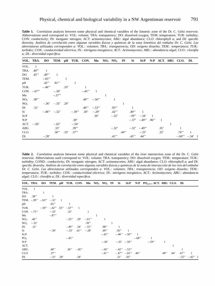
Physical, chemical and biological variability in a NW Argentinean reservoir 791
Table 1. Correlation analysis between some physical and chemical variables of the limnetic zone of the Dr. C. Gelsi reservoir.Abbreviations used correspond to: VOL: volume; TRA: transparency; DO: dissolved oxygen; TEM: temperature; TUR: turbidity;CON: conductivity; IN: inorganic nitrogen; ACT: actinomycetes; ABU: algal abundance; CLO: chlorophyll a; and DI: specificdiversity. Analisis de correlacion entre algunas variables fisicas y quımicas de la zona limnetica del embalse Dr. C. Gelsi. Lasabreviaturas utilizadas corresponden a: VOL.: volumen; TRA.: transparencia; OD: oxıgeno disuelto; TEM.: temperatura; TUR.:turbidez; CON.: conductividad electrica; IN.: nitrogeno inorganico; ACT.: Actinomycetes; ABU.: abundancia algal; CLO.: clorofilaa; DI.: diversidad especıfica.
VOL. TRA. DO TEM. pH TUR. CON. Mn NO3 NO2 IN Si Si:P N:P ACT. ABU. CLO. DI.
VOL. 1TRA. .40∗∗ 1DO .45∗∗ .49∗∗ 1TEM. −.65∗∗ 1pH .42∗∗ .81∗∗ 1
TUR. −.46∗∗ .33∗ 1CON. −.67∗∗ −.30∗ −.45∗∗ 1Mn −.57∗∗ 1NO3 .38∗∗ .40∗∗ −.56∗∗ 1NO2 −.36∗ −.35∗ .29∗ 1IN .31∗ .40∗∗ −.53∗∗ .93∗∗ 1Si −.48∗∗ −.32∗ −.39∗∗ .30∗ −.29∗ .42∗∗ .49∗∗ 1Si:P .30∗ −.32∗ −39∗∗ −.34∗ 1N:P .30∗ −.37∗ −.49∗∗ .96∗∗ 1ACT. −.56∗ −.62∗ −.54∗ 1ABU. .33∗ .39∗∗ −.32∗ −.32∗ −.49∗∗ .35∗ 1CLO. .36∗∗ .33∗ .37∗∗ .44∗∗ −.33∗ .32∗ .74∗∗ 1DI. −.28∗ .41∗∗ .45∗∗ .44∗∗ −.60∗∗ −.34∗ 1
Table 2. Correlation analysis between some physical and chemical variables of the river intersection zone of the Dr. C. Gelsireservoir. Abbreviations used correspond to: VOL: volume; TRA: transparency; DO: dissolved oxygen; TEM.: temperature; TUR.:turbidity; COND.: conductivity; IN: inorganic nitrogen; ACT: actinomycetes; ABU: algal abundance; CLO: chlorophyll a; and DI:specific diversity. Analisis de correlacion entre algunas variables fisicas y quımicas de la zona de interseccion de los rıos del embalseDr. C. Gelsi. Las abreviaturas utilizadas corresponden a: VOL.: volumen; TRA.: transparencia; OD: oxıgeno disuelto; TEM.:temperatura; TUR.: turbidez; CON.: conductividad electrica; IN.: nitrogeno inorganico; ACT.: Actinomycetes; ABU.: abundanciaalgal; CLO.: clorofila a; DI.: diversidad especıfica.
VOL. TRA. DO TEM. pH TUR. CON. Mn NO3 NO2 IN Si Si:P N:P POpetb 4 ACT. ABU. CLO. DI.
VOL. 1TRA. 1DO .38∗∗ 1TEM. −.39∗∗ −.63∗∗ −.31∗ 1pH .65∗∗ 1TUR. −.59∗∗ −.42∗∗ .55∗∗ −.67∗∗ 1CON. −.73∗∗ −.33∗ .32∗ 1Mn −.87∗∗ 1NO3 .40∗∗ −.35∗∗ .29∗ −.61∗∗ 1NO2 −.32∗ .39∗∗ 1IN .31∗ −.40∗∗ .34∗ −.55∗∗ .98∗∗ 1Si −.30∗ −.33∗ .41∗∗ −.28∗ .49∗∗ .56∗∗ 1Si:P −.42∗∗ −.46∗∗ −.50∗∗ 1PO4 −.45∗∗ −.68∗∗ 1N:P −.30∗ −.35∗ −.59∗∗ −.59∗∗ 1ACT. 1ABU. .40∗∗ .36∗∗ −.36∗∗ −.36∗∗ −.42∗∗ −.53∗∗ 1CLO. .37∗∗ −.41∗∗ −.47∗∗ −.65∗∗ .46∗∗ .49∗∗ .64∗ .67∗∗ 1DI. −.31∗ .30∗ .34∗ .31∗ .56∗∗ −.55∗∗ −.42∗∗ 1

792 Tracanna et al.
Figure 2. Variations of water level, flow, and volume (1997-1999) in the Dr. C. Gelsi reservoir. Variaciones de cota, caudal yvolumen (1997-1999) del embalse Dr. C. Gelsi.
and Peridinium volzii in ZIR were also inclu-ded. In order to establish correlations betweenpairs of variables, Pearson’s correlation coef-ficient was used. Data were processed usingthe NTSYS (Rolf, 1990) statistical package.
A correlation statistical analysis (Pearson’scoefficient) between physical, chemical and bio-logical variables was performed, and the firstthree PCA components effected with algal den-sities by using the SPSS program were included.In this work the correlations that proved to be sig-nificant ( p <0.05 and p <0.01) are explained.
RESULTS
Variations in water level, volume, and flow(October/97-March/99) (Fig. 2) showed that thefirst two parameters had their minimal recordsin December/98 with 592.40 m a.s.l.and 94.40hm3 and their maximal records in April/98 with607.62 m a.s.l. and 218.05 hm3, respectively. Re-garding flow, the minimum was observed in No-vember/97 with 1.98 m3/s and the maximum inMarch/99 with 78.63 m3/s.
Maximal Secchi’s disk depths (Fig. 3) weregenerally obtained from March to October 1998,ranging between 1.2 and 2.47 in ZI, and between1.27 and 2 m in ZIR. Minimal values registeredfor both sites were 0.17-0.23 m. Transparencyhad a highly significant positive correlation with
volume, dissolved oxygen, and pH, a negativecorrelation with temperature, turbidity, and silicadioxide, a significant negative correlation withnitrite, a specific diversity in ZI, and a highlysignificant negative correlation with temperatureand turbidity in ZIR (Tables 1 and 2).
Annual thermal behavior defines the reservoiras monomictic, with a stratification period fromOctober to February, with the beginning of themixing period in March. The highest temperaturedifference was observed in ZI in December/97and in October/98, with a thermocline between 5and 10 m deep, a 5 ◦C decrease being registered.In ZIR, stratification was less evident due to itslower depth and water flow because this is aconfluence zone of the rivers.
The concentration of hydrogen ions was,in general, slightly higher on the surface thanin depth layers in both sampling sites, thisdifference being higher in the stratificationperiod. PH records in ZI ranged between 8.87in October/97 (on the surface) and 7.78 inNovember and December/97 (at a depth of 35m), whereas in ZIR they ranged between 8.86in October/97 (on the surface) and 7.50 inMarch/99 (at a depth of 10 m).
Maximal ZI and ZIR values of conductivitywere 1520 µS/cm at December/97, on the surfacefor both and in November/97, at a depth of 5 monly for ZIR; minimal conductivity values were505 µS/cm for ZI, and 541 µS/cm for ZIR, both in

Physical, chemical and biological variability in a NW Argentinean reservoir 793
Table 3. Number of observations, minimal, maximal, and average values, and standard deviations of cations, anions, nitrogencompounds, and orthophosphate from October 1997 to March 1999 in the two zones considered. Numero de observaciones, mınimos,maximos, promedios y desviaciones estandares de los cationes, aniones, compuestos nitrogenados y ortofosfato desde octubre de1997 a marzo de 1999 en las dos zonas consideradas.
Variables (mg/l) ZI ZIR
n min. max. X sd n min. max. X sdCarbonate 54 0 30 3 6 54 0 36 3 5Bicarbonate 54 112 189 159 18 54 112 180 158 17Sulfate 54 41 237 109 55 54 49 229 103 43Chloride 33 46 214 140 41 33 64 214 140 38Sodium 43 46 260 139 40 43 55 219 140 38Potassium 43 3 10 5 1 43 4 8 5 1Calcium 54 4 80 29 21 54 4 63 23 18Magnesium 36 3 47 24 13 36 5 46 25 10Silica dioxide 54 7 22 16 3 54 7 22 15 3Total manganese 54 <0.02 0.7 0.2 0.2 54 <0.02 0.6 0.1 0.1Inorganic nitrogen 54 0.76 1.86 1.19 0.26 54 0.8 1.8 1.2 0.3Nitrate 54 0.6 1.84 1.12 0.27 54 0.7 1.8 1.2 0.3Nitrite 54 <0.01 0.5 0.06 0.09 54 <0.01 0.2 0.03 0.03Ammonium 54 <0.05 0.09 0.06 0.02 54 <0.05 0.13 0.06 0.03Orthophosphate 54 <0.004 15.6 0.45 2.31 54 <0.004 0.28 0.12 0.06Si:P 44 2 1742 437 439 45 107 1583 308 253N:P 44 0.1 184 31 36 45 7 169 24 25
Abbreviations: n = number of observations; min. = minimum; max. = maximum; X = average; sd = standard deviation
March/99, at the bottom. It was observed that thetemporal-spatial conductivity value profiles dimi-nish with depth; however an evident increase ofthese values was detected in the hypolimnion inJanuary and February/98-99 for ZI and ZIR, andin November/98 only for ZIR. The time evolu-tion of the average value of conductivity in thewater column for both sites is observed in figure5. Minimal registers at the end of summer/98 and99 and fall/98 gradually increase in the beginningof summer. In ZI significant positive correlationswith Si:P were obtained, highly significant nega-tive correlations were found with volume, turbi-dity, nitrate, inorganic nitrogen, and significantones with DO and silica dioxide; in ZIR highlysignificant positive correlations were found withnitrite, significant ones with pH, highly signifi-cant negative correlations with nitrate, volume,and inorganic nitrogen, and significant ones withDO and silica dioxide (Tables 1 and 2).
Turbidity (as National Units of Turbidity(NUT)) ranged between 1.6 in September/98(on the surface) and 53.6 in March/99 (at thebottom) in ZI, and between 0 for December/98(on the surface) and 47.9 in December/97 (at adepth of 10 m) in ZIR.
The distribution of dissolved oxygen concen-
tration in the profile was closely related to thestratification and mixing periods (Fig. 4). Ma-ximal DO values were obtained on the surfacein November/98 with 10.26 mg/l in ZI and inJuly/98 with 10.65 mg/l in ZIR. Minimal recordswere obtained at the bottom, 0.03 mg/l beingin December/97 and January/98 in ZI, and 0.07mg/l in November/97 in ZIR. The highest diffe-rences between surface and bottom (8 mg/l) wereregistered in November and December/97-98 andJanuary/98-99 in ZI and (9 mg/l) in November/97in ZIR. During that period the curve of DO dis-tribution was clinograde-type.
Table 3 shows minimal, maximal, and averagevalues and standard deviations of anions, cations,nitrogenous compounds, and orthophosphate forthe study period.
Ionic concentrations at the different levels stu-died did not show marked differences, the waterbeing characterized, according to ion prevalence,as bicarbonated, chlorinized, sodic, calcic and/ormagnesic. Anion seasonal distribution in the lim-netic zone revealed some differences in winterwhere the order changed into sulphated, bicarbo-nated and chlorinized.
Figure 4 shows the vertical profiles of tempe-rature, pH, conductivity, and dissolved oxygen

794 Tracanna et al.
Figure 3. A-B. Transparency in the studied sites in the Dr. C. Gelsi reservoir. A-B Transparencia en los sitios estudiados del embalseDr. C. Gelsi. A: ZI, B: ZIR.
for the limnetic zone (ZI) in December/97-98and in June/98, these months being those thatgenerally encompass time and space variationsin such variables.
The rate of inorganic nitrogen in the sites stu-died was, in general, higher than 1 mg/l, reaching1.9 mg/l in May/98. Nitrate values were similar atthe different depths considered, with the excep-tion of what had happened in the hypolimnionin January and February 1998 and January/99where a marked decrease was observed. Nitritemaximal records reached 0.5 and 0.2 mg/l in ZIin February/99 (on the surface) and in ZIR inFebruary/98 (at the bottom), respectively, corres-ponding to the reservoir stratification period, andreaching values of <0.01 mg/l during the mixingperiod. Ammonium showed a remarkable timeand space fluctuation in ZI ranging between non-detectable and 0.09 mg/l at a depth of 10 m inFebruary/98. In the case of ZIR, maximal varia-tions occurred in spring 1997 and summer 1998reaching 0.1 mg/l in February/98 (at the bottom)and then generally maintaining below 0.05 mg/l.
Orthophosphate concentrations reached ma-ximal values in ZI in October/97 in the hy-
polimnion reaching 15.6 mg/l. This value was80 times higher with respect to the otherdepths. In general the average values of the stu-died monthly profiles in both sites were nothigher than 0.2 mg/l, moreover, orthophospha-tes were no detected in some samples. Theorthophosphates did not have any correlationwith the studied parameters in ZI, however thisanion had highly significant negative correlationswith some parameters in ZIR (Table 2).
Nitrogen and phosphorus concentrations inthe water show approximately the same relativeratios found in living matter, where a 14-16:1 ra-tio in atoms is kept (Margalef, 1983). This ra-tio only coincided in 13 % and 17 % of thesamples in ZI and ZIR, respectively. The rela-tion was higher in 45 % of the samples reaching211 on the surface of ZI in October/98 due tothe nearly total absence of soluble orthophos-phate and with no ratio in non-detected cases.Tables 1 and 2 showed the highly significantand significant correlations obtained for the ni-trate:orthophosphate ratio (N:P ratio).
Average values for silica dioxide concentra-tions in both zones were higher in the summer

Physical, chemical and biological variability in a NW Argentinean reservoir 795
Figure 4. Behavior of temperature, pH, DO, and conductivity in the limnetic zone of the Dr. C. Gelsi reservoir in the mixing andstratification periods. Comportamiento de la temperatura, pH, OD y conductividad electrica en la zona limnetica en los perıodos demezcla y estratificacion del embalse Dr. C. Gelsi.
Figure 5. Conductivity average changes through the time inthe water column for the limnetic and tributary intersectionzones (ZI: white triangle and ZIR: black square symbols).Evolucion en el tiempo del valor promedio de la conductividaden la columna de agua para la zona limnetica y la zona deinterseccion de los tributarios (sımbolos: triangulo blanco ZIy cuadrado negro ZIR).
of 1998, they decreased until the end of winter,and after their spring recovery they decreasedreaching the lowest values in January 1999. TheSi:P ratio in about 70 of the samples was largerthan 200 and ranged between 100 and 200 theremainder samples except in October/98 that it
was 2 at the bottom of ZI. The highest ratios oc-curred during the mixing period, and in October-November/98 and January/99.
Total manganese was higher at the bottomthan on the surface in both zones for the two stra-tification periods studied. In the first one, ma-ximal values reached 0.7 and 0.6 mg/l in Ja-nuary/98 in ZI and ZIR, respectively, whereas inthe second one they were 0.2 mg/l in October/98in ZI, and 0.3 mg/l in February/99 in ZIR. Overthe circulation period, manganese was not detec-ted along the whole water column. Highly signifi-cant negative correlations with dissolved oxygenin both zones (Tables 1 and 2) were found.
Out of the eleven organochlorine pesticidesstudied, DDT and dieldrin isolated values wereobserved for ZIR, whereas practically throughoutthe whole period the presence of lindane and me-thoxychlor with higher values in warm monthswas detected. The highest average values forthe two last ones in the first half of the year(April-September 1998) were 0.05 and 0.02µg/l, respectively, whereas from September/98 to

796 Tracanna et al.
March/99 average values increased to 0.39 and0.18 µg/l. A similar seasonal behavior was obser-ved in ZI, but the maximal values reached werelower than in ZIR with average values of 0.21 and0.19 µg/l for lindane and methoxychlor, respecti-vely, during the second summer period.
The organic matter values ranged from 1.47% in November/98 to 1.54 % in February/98 inZI, whereas in ZIR they varied between 1.49 %and 1.50 % in every sediment sample studied.
The maximal value for total coliforms in bothsampling sites was four logarithmic units in Fe-bruary/98. Fecal streptococci figures reached 8
and 9 UFC/100 ml in October/97 and May/98 inZI, whereas in ZIR they only reached 8 UFC/100ml in November/97.
The number of actinomycetes coloniesranged between 3 in April/98 and 272 inOctober/98 in ZI, whereas in ZIR it rangedbetween 8 and 94 in December 1997 and1998, respectively, a negative correlation withdissolved oxygen in ZI (Table 1), and apositive correlation with DO in ZIR (Table 2)was obtained among other parameters.
The species phytoplankton richness (Table 4)in ZI was represented by 50 species: 26 Chlo-
Figure 6. A-F. Variations of the main algal groups and total density of the Dr. C. Gelsi reservoir. A-C. In the limnetic zone: A.surface, B. 10 m, C. bottom, D-F. intersection zone of tributaries, D. surface, E. 5 m, F. bottom. A-F. Variaciones de los principalesgrupos algales y la densidad total del embalse Dr. C. Gelsi. A-C. en la zona limnetica: A. superficie, B. 10 metros, C. fondo. D-F.zona de interseccion de los rıos. D. superficie, E. 5 metros, F. fondo.
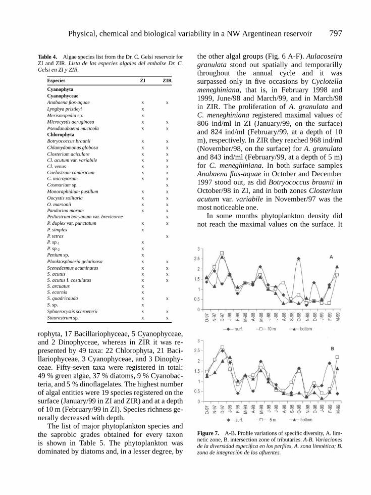
Physical, chemical and biological variability in a NW Argentinean reservoir 797
Table 4. Algae species list from the Dr. C. Gelsi reservoir forZI and ZIR. Lista de las especies algales del embalse Dr. C.Gelsi en ZI y ZIR.
Especies ZI ZIR
CyanophytaCyanophyceaeAnabaena flos-aquae x xLyngbya pristleyi xMerismopedia sp. xMicrocystis aeruginosa x xPseudanabaena mucicola x xChlorophytaBotryococcus braunii x xChlamydomonas globosa x xClosterium aciculare x xCl. acutum var. variabile x xCl. venus x xCoelastrum cambricum x xC. microporum x xCosmarium sp. xMonoraphidium pusillum x xOocystis solitaria x xO. marsonii x xPandorina morum x xPediastrum boryanum var. brevicorne xP. duplex var. punctatum x xP. simplex xP. tetras xP. sp.1 xP. sp.2 xPenium sp. xPlanktosphaeria gelatinosa x xScenedesmus acuminatus x xS. acutus x xS. acutus f. costulatus x xS. arcuatus xS. ecornis xS. quadricauda x xS. sp. xSphaerocystis schroeterii x xStaurastrum sp. x x
rophyta, 17 Bacillariophyceae, 5 Cyanophyceae,and 2 Dinophyceae, whereas in ZIR it was re-presented by 49 taxa: 22 Chlorophyta, 21 Baci-llariophyceae, 3 Cyanophyceae, and 3 Dinophy-ceae. Fifty-seven taxa were registered in total:49 % green algae, 37 % diatoms, 9 % Cyanobac-teria, and 5 % dinoflagelates. The highest numberof algal entities were 19 species registered on thesurface (January/99 in ZI and ZIR) and at a depthof 10 m (February/99 in ZI). Species richness ge-nerally decreased with depth.
The list of major phytoplankton species andthe saprobic grades obtained for every taxonis shown in Table 5. The phytoplankton wasdominated by diatoms and, in a lesser degree, by
the other algal groups (Fig. 6 A-F). Aulacoseiragranulata stood out spatially and temporarillythroughout the annual cycle and it wassurpassed only in five occasions by Cyclotellameneghiniana, that is, in February 1998 and1999, June/98 and March/99, and in March/98in ZIR. The proliferation of A. granulata andC. meneghiniana registered maximal values of806 ind/ml in ZI (January/99, on the surface)and 824 ind/ml (February/99, at a depth of 10m), respectively. In ZIR they reached 968 ind/ml(November/98, on the surface) for A. granulataand 843 ind/ml (February/99, at a depth of 5 m)for C. meneghiniana. In both surface samplesAnabaena flos-aquae in October and December1997 stood out, as did Botryococcus braunii inOctober/98 in ZI, and in both zones Closteriumacutum var. variabile in November/97 was themost noticeable one.
In some months phytoplankton density didnot reach the maximal values on the surface. It
Figure 7. A-B. Profile variations of specific diversity, A. lim-netic zone, B. intersection zone of tributaries. A-B. Variacionesde la diversidad especıfica en los perfiles, A. zona limnetica; B.zona de integracion de los afluentes.

798 Tracanna et al.
Figure 8. A-B. Average values of chlorophyll a, phytoplank-ton biomass and density in the Dr. C. Gelsi reservoir. A. limne-tic zone; B. intersection zone of tributaries. A-B. Valores pro-medios de clorofila a, biomasa y densidad del fitoplancton delembalse Dr. C. Gelsi: A. zona limnetica (ZI); B. zona de inter-seccion de los tributarios (ZIR).
was higher in the deep in April, May, Augustand October/98 in ZI; it was similar only inOctober/98 in ZIR.
Species diversity (Fig. 7 A and B) rangedbetween 0.2 (November/98, on the surface) and2.8 (December/97, at a depth of 10 m) in ZI,while in ZIR it ranged between 0.1 (January/99,at the bottom) and 2.7 (December/97, at a depthof 5 m). This index showed low values in winterand in November-December/98 and January/99(summer) due to a marked growth of A. granulataand C. meneghiniana.
Figure 8 (A-B) represents the average valuesof algal density, biomass, and chlorophyll a bothin ZI and ZIR. The number of average indivi-duals/ml in the water column ranged between 16(March/99) and 531 (February/99) in ZI, whe-reas in ZIR it ranged between 27 (March/99) and655 (November/98). The highest average bio-mass values on the vertical profile for both sam-
pling sites occurred in July-September/98 and inNovember/98-January/99. These records rangedbetween 2.15 and 7.4 mg/l, while in the othermonths they did not exceed 1.7 mg/l. The bio-mass values in both sites, increased in the deepin the same months as the phytoplankton density.The highest difference among the three levels ap-peared in ZI during the 98-99 summer stratifica-tion, being higher in January with values of 9.2,6.7 and 1.2 mg/l on the surface, at a depth of 10 mand at the bottom, respectively.
The biomass percentage in ZI correspondingto the surface was 64 % for diatoms, 22 % forgreen algae, 13 % for cyanobacteria, and 1 %for dinoflagelates. Cyanobacteria only prevailedin October and December/97, and were subdo-
Table 5. List of the most abundant species and their sa-probic grades obtained for the Dr. Gelsi reservoir. 1: oligo-β-mesosaprobic (s: 1.5); 2: β-α-mesosaprobic (s: 2.5), 3: α-mesosaprobic (s: 3). (∗) The eleven species coincide with thosefor the 1988-1989 period. Lista de especies mayoritarias y susgrados saprobicos obtenidos para el embalse Dr. C. Gelsi. 1:oligo-β-mesosaprobias (s: 1.5), 2: β-α-mesosaprobias (s: 2.5),3: α-mesosaprobias (s: 3). (∗) Las once especies son coinciden-tes con las del perıodo 1988-1989.
1 2 3
CyanophytaCyanophyceae(∗) Anabaena flos−aquae (Lyngbye) Brebisson x
(∗) Microcystis aeruginosa Kutzing x
Chlorophyta(∗)Botryococcus braunii Kutzing x
Closterium aciculare West x(∗) Closterium acutum var. variabile(Lemmermann) Krieger x
(∗) Closterium venus Kutzing x
(∗) Coelastrum microporum Naegeli x
(∗) Oocystis solitaria Wittrock xOocystis marsonii Lemmermann x
(∗) Planktosphaeria gelatinosa G. M. Smith x
(∗) Sphaerocystis schroeteri Chodat xStaurastrum sp. x
DinophytaDinophyceaeGlochidinium penardiforme (Lindemann)Boltovskoy x
Peridinium volzii Lemmermann xPeridinium willei Huitfeld−Kaas xHeterokontophytaBacillariophyceae(∗) Aulacoseira granulata (Ehrenberg) Simonsen x
(∗) Cyclotella meneghiniana Kutzing x

Physical, chemical and biological variability in a NW Argentinean reservoir 799
Figure 9. A-D. Principal Components Analysis (PCA) of the limnetic zone of the Dr. C. Gelsi reservoir in relation to phytoplanktondensity and some physical and chemical variables. A-B: graphic representation of Components 1 and 2; C-D. Graphic representationof Axes 1 and 3. Abbreviations used for species are: Anabaena flos-aquae (Afl), Aulacoseira granulata (Ag), Botryococcus braunii(Bb), Closterium aciculare (Cla), Closterium acutum var. variabile (Clav), Closterium venus (Clv), Cyclotella meneghiniana (Cym),Glochidinium penardiforme (Gp), Microcystis aeruginosa (Ma), Oocystis marsonii (Om), Oocystis solitaria (Os), Peridinium willei(Pw), Planktosphaeria gelatinosa (Pg), Sphaerocystis schroeteri (Ss), and Staurastrum sp. (St); abbreviations used for physical andchemical variables are: conductivity (Cond), biological oxygen demand (BOD5), nitrate (N0−3 ), orthophosphate (PO4), dissolvedoxygen (DO), hydrogen potential (pH), and temperature (Temp); symbols for the periods studied Fig. 9 A are: October/97-March/98 stratification (rhombi: white, surface; gray, 10 meters, and black, bottom), April/98-September/98 mixture (ellipses: white,surface; gray, 10 meters, and black, bottom), October/98-March/99 stratification (triangles: white, surface; gray 10 meters, andblack, bottom); Fig. 9 C: October/97-March/98 stratification (rhombi white), April/98-September/98 mixture (ellipses white), andOctober/98-March/99 stratification (triangles black). A-D. Analisis de componentes principales (ACP) de la zona de limnetica (ZI)del embalse Dr. C. Gelsi en relacion con la densidad del fitoplancton y algunas variables fısicas y quımicas: A-B. Representacionde los Componentes 1 y 2; C-D. Representacion de los Ejes 1 y 3. Las abreviaturas usadas para las especies son: Anabaena flos-aquae (Afl), Aulacoseira granulata (Ag), Botryococcus braunii (Bb), Closterium aciculare (Cla), Closterium acutum var. variabile(Clav), Closterium venus (Clv), Cyclotella meneghiniana (Cym), Glochidinium penardiforme (Gp), Microcystis aeruginosa (Ma),Oocystis marsonii (Om), Oocystis solitaria (Os), Peridinium willei (Pw), Planktosphaeria gelatinosa (Pg), Sphaerocystis schroeteri(Ss), Staurastrum sp. (St); abreviaturas utilizadas para las variables fısicas y quımicas: conductividad electrica (Cond), demandabioquımica de oxıgeno (DBO5), nitrato (NO−3 ), ortofosfato (PO4), oxıgeno disuelto (OD), potencial hidrogeno (pH), temperatura(Temp); sımbolos de los perıodos estudiados, Fig. 9 A: estratificacion octubre/97-marzo/98 (rombos: blanco, superficie; gris, 10metros y negro, fondo), mezcla abril/98-setiembre/97 (elipses: blanca, superficie; gris, 10 metros y negra, fondo), estratificacionoctubre/98-marzo/99 (triangulos: blanco, superficie; gris, 10 metros y negro, fondo); Fig. 9 C: estratificacion octubre/97-marzo/98(rombos blancos), mezcla abril/98-setiembre/97 (elipses blancas), estratificacion octubre/98-marzo/99 (triangulos negros).
800 Tracanna et al.
minant in January, February, and October 1998and February 1999.Chlorophyta prevailed in Mayand October 1998 and March/99. In ZIR, also onthe surface, the biomass percentage was 78 % fordiatoms, 16 % for green algae, 5 % for cyanobac-teria, and 1 % for dinoflagelates. Bacillariophy-ceae were dominant except in November and De-cember 1997 when Chlorophyta prevailed. Cya-nobacteria were subdominant in February andMay 1998 and February 1999. At other levelsdiatoms stood out and they were seldom surpas-sed by green algae.
Concentrations of chlorophyll a revealed adecrease with depth in most of the period studiedin both zones, their average values increasedfrom winter to summer 1999. Both in ZI and ZIR,hypolimnion concentrations were detected lowerthan 1.2 µg/l from October 1997 to May 1998.Maximal values were obtained on the surfacewith 63 µg/l for ZI in February 1999, whereasin ZIR they were 35 µg/l in November 1998.The obtained correlations for the chlorophyll areshowed in Tables 1 and 2.
It is important to notice that the results ofphytoplankton density and chlorophyll a at depthcome from a wide range of values obtained. Thiscould be the reason that a positive correlationbetween these two parameters was gotten, even ifreduction in the phytoplankton density was onlydetected in some months.
The saprobic index that ranged between 2.5and 3, characterized the reservoir water qualityas β-α-mesosaprobic with records of biochemi-cal oxygen demand lower than 7 mg/l to α-mesosaprobic with BOD5 values lower than 13mg/l. In some samples, the saprobic index did notagree with the organic matter, thus in ZI in De-cember 1997 waters were b-mesosaprobic withBOD5 values of 11 mg/l, whereas in June 1998and September 1998 they were α-mesosaprobicwith BOD5 rate of 17 to 19 mg/l.
In the PCA for ZI, the first four componentsaccounted for 58 % of data variability, the firstthree axes being responsible for 18 %, 15 %, and13 % of the total variance. Component 1 ordina-ted towards the negative portion such as the bot-tom samples for both stratification periods, andthose of the first months of the mixing period
(Fig. 9 A). Abiotic variables of axis 1 that contri-buted to this ordination were pH, dissolved oxy-gen, nitrate, and conductivity (intra-set correla-tion coefficients: 0.71; 0.46; −0.46, and 0.42, res-pectively). The algae that accounted for most ofthe distribution of the samples were C. acutumvar. variabile, A. granulata, Glochidinium penar-diforme, and Staurastrum sp. (intra-set correla-tion coefficients: 0.69; 0.68; 0.59 and 0.55, res-pectively) (Fig. 9 B).
With regards to component 2, it revealed a sig-nificant correlation with a few environmental va-riables and separated the ’97-’98 stratification to-wards the negative portion, and that of ’98-’99period towards the positive one. Mixing monthswere arranged between the previously mentionedperiods (Fig. 9 A). The algae that most contri-buted to the arrangement regarding component 2were Anabaena flos-aquae, Planktosphaeria ge-latinosa and Sphaerocystis schroeteri (intra-setcorrelation coefficients: −0.80, −0.73, and −0.64,respectively) (Fig. 9 B).
Component 3 arranged the samples of the mi-xing period towards the positive quadrant andthose of both stratifications were, in general, lo-cated negatively. The abiotic variables of axis 3that contributed to the sample distribution wereconductivity, temperature, dissolved oxygen, andnitrate (intra-set correlation coefficients: −0.55;−0.54; 0.51; 0.40, respectively). Prevalent al-gae were B. braunii and C. meneghiniana (intra-set correlation coefficients: −0.69; 0.46, respecti-vely) (Fig. 9 C and D).
In the PCA for ZIR, the first four compo-nents were found to account for 55 % of datavariability, the first three axes being responsi-ble for 21 %, 12 %, and 11 % of the total va-riance. In figure 10 A, in relation to components1 and 2, it was observed how variables arran-ged most months of the ’98-’99 stratification pe-riod on the surface and at a depth of 5 m to-wards the upper quadrants, and towards the lo-wer quadrants those of the mixing period andthose of some months of the ’97-’98 stratifica-tion. The remaining samples of the latter periodwere found spread in the positive sector of com-ponent 2 and those at the bottom of those stra-tifications were located in the negative portion

Physical, chemical and biological variability in a NW Argentinean reservoir 801
Figure 10. A-D. Principal Components Analysis (PCA) of the tributaries intersection zone of the Dr. C. Gelsi reservoir in relationto phytoplankton density and some physical and chemical variables: A-B. Graphic representation of Components 1 and 2; C-D.Graphic representation of Axes 1 and 3. The abbreviations used for species and physical and chemical variables are the same asin figure 9. Symbols for the studied periods Fig. 10 A: October/97-March/98 (rhombi: white, surface; gray, 5 meters, and black,bottom), April/98-September/98 mixing period (ellipses: white, surface; gray, 5 meters, and black, bottom), October/98-March/99stratification period (triangles: white, surface; gray, 5 meters, and black, bottom); Fig. 10 C: October/97-March/98 stratification(rhombi white), April/98-September/98 mixture (ellipses white), October/98-March/99 stratification (triangles black). A-D. Analisisde componentes principales (ACP) de la zona de integracion de los afluentes (ZIR) del embalse Dr. C. Gelsi en relacion con ladensidad del fitoplancton y algunas variables fısicas y quımicas: A-B. Representacion de los Componentes 1 y 2; C-D. Representacionde los Ejes 1 y 3. Las abreviaturas usadas para las especies y las variables fısicas y quımicas son las mismas que en la figura 9.Sımbolos de los perıodos estudiados Fig. 10 A: estratificacion octubre/97-marzo/98 (rombos: blanco, superficie; gris, 5 metros ynegro, fondo), mezcla abril 98-setiembre/97 (elipses: blanca, superficie; gris, 5 metros y negra, fondo), estratificacion octubre/98-marzo/99 (triangulos: blanco, superficie; gris, 5 metros y negro, fondo); Fig. 10 C: estratificacion octubre/97-marzo/98 (rombosblancos), mezcla abril/98-setiembre/97 (elipses blancas), estratificacion octubre/98-marzo/99 (triangulos negros).

802 Tracanna et al.
of component 2. The abiotic parameters of com-ponent 1 that contributed to this arrangementwere pH, orthophosphate, nitrate, conductivity,and DO (intra-set correlation coefficients: 0.76,−0.75, −0.58, 0.50, and 0.40, respectively).Those of component 2 were temperature(intra-set correlation coefficients: 0.47), whereasthe algae that most contributed, either due totheir density or to their space correlation inthe distribution of samples were in the firstcomponent A. granulata, Oocystis solitaria, andC. acutum var. variabile (intra-set correlationcoefficients: 0.88, 0.80 and 0.62, respectively),and in component 2 Microcystis aeruginosa,Anabaena flos-aquae, and G. penardiforme(intra-set correlation coefficients: 0.68, 0.65, and0.63, respectively) (Fig. 10 B). Component 3(Figs. 10 C and D) exhibited a low correlationwith environmental variables, whereas the algaethat contributed to sample distribution wereClosterium venus, C. meneghiniana, and Peri-dinium volzii (intra-set correlation coefficients:−0.65, −0.55 and 0.53, respectively).
DISCUSSION AND CONCLUSIONS
Marked variations of hydrological behaviorthroughout the 18 months studied determined mi-nimal volumes in spring and maximal volumes insummer-autumn. The delay of the rainy summerperiod in the ’97-’98 period resulted in low waterlevels (Fig. 2) coincident with those of the 1987-’88 period (Tracanna et al., 1991).
Low values for transparency are mainly dueto the turbidity caused by the increase ofsuspended solids in rainy periods in accordancewith what was observed by Ferrer et al., 2000,among other authors, that assert that the lowtransparency registered for a reservoir shouldnot always be attributed to the developmentof algal communities.
From a thermal viewpoint the reservoir wascharacterized as a warm monomictic-type lake,that is, it shows only one relatively longannual circulation period (April-September)with temperatures always higher than 4 ◦C,a category which most northern and central
Argentine reservoirs belong to (Locascio et al.,1997, among others).
Waters are alkaline, a characteristic caused bythe chemical composition of basin rocks that ex-hibit a prevalence of bicarbonate. From Octoberto March pH records were higher on the surfacethan at the bottom.
Conductivity reached high values in relationwith other studies conducted in Argentine reser-voirs (Arjona et al., 2000, Bonetto et al., 1976,among others).
Conductivity measurement allows for the ap-proximate assessment of global water minerali-zation. According to general average values ofconductivity, and taking into account the FrenchRegulation (Rodier, 1990) that estimates the ra-tio between mineralization and conductivity, thewaters were classified as ones with excessive mi-neralization since they exceed 1100 µS/cm. In the1987-’89 period the waters were significantly mi-neralized because the conductivity did not excee-ded 900 µS/cm (Tracanna et al., 1991).
Dissolved oxygen determinations were about0 mg/l in the deep from November to Januarycoinciding with the reservoir heterothermy, theybeing homogeneous from March onwards in thewhole water column.
According to ion prevalence, reservoir waterscould be characterized as bicarbonated (26 %),chlorinized (23 %), sodic (23 %), calcic (5-3.8 %), and/or magnesic (4 %). Sometimessulphate values surpassed those of bicarbonatesby insignificant differences. Marked differenceswere not observed between ionic concentrationsat the intersection river zone and the limneticzone among the various levels considered. Theseresults could indicate that the conductivitydifference found is produced by water level andrains instead of ionic changes.
The decrease of nitrate in the bottom duringthe stratification period coincides with the in-crease of nitrite and ammonium. This result is aconsequence of the anoxic conditions.
Nitrogen, phosphorus, and silica inorganicforms mainly behave as nutrients, and theirevaluation is important for the interpretation ofthe organisms distribution and annual cycles.The same can be said for the assessment
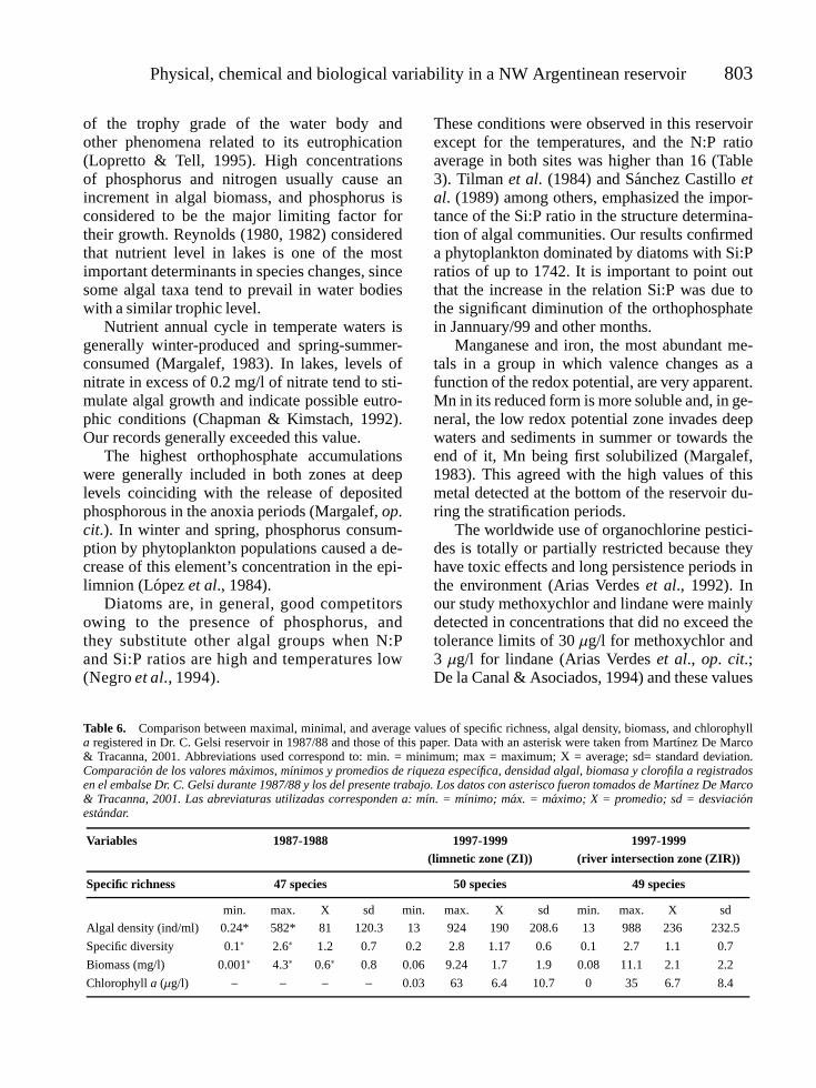
Physical, chemical and biological variability in a NW Argentinean reservoir 803
of the trophy grade of the water body andother phenomena related to its eutrophication(Lopretto & Tell, 1995). High concentrationsof phosphorus and nitrogen usually cause anincrement in algal biomass, and phosphorus isconsidered to be the major limiting factor fortheir growth. Reynolds (1980, 1982) consideredthat nutrient level in lakes is one of the mostimportant determinants in species changes, sincesome algal taxa tend to prevail in water bodieswith a similar trophic level.
Nutrient annual cycle in temperate waters isgenerally winter-produced and spring-summer-consumed (Margalef, 1983). In lakes, levels ofnitrate in excess of 0.2 mg/l of nitrate tend to sti-mulate algal growth and indicate possible eutro-phic conditions (Chapman & Kimstach, 1992).Our records generally exceeded this value.
The highest orthophosphate accumulationswere generally included in both zones at deeplevels coinciding with the release of depositedphosphorous in the anoxia periods (Margalef, op.cit.). In winter and spring, phosphorus consum-ption by phytoplankton populations caused a de-crease of this element’s concentration in the epi-limnion (Lopez et al., 1984).
Diatoms are, in general, good competitorsowing to the presence of phosphorus, andthey substitute other algal groups when N:Pand Si:P ratios are high and temperatures low(Negro et al., 1994).
These conditions were observed in this reservoirexcept for the temperatures, and the N:P ratioaverage in both sites was higher than 16 (Table3). Tilman et al. (1984) and Sanchez Castillo etal. (1989) among others, emphasized the impor-tance of the Si:P ratio in the structure determina-tion of algal communities. Our results confirmeda phytoplankton dominated by diatoms with Si:Pratios of up to 1742. It is important to point outthat the increase in the relation Si:P was due tothe significant diminution of the orthophosphatein Jannuary/99 and other months.
Manganese and iron, the most abundant me-tals in a group in which valence changes as afunction of the redox potential, are very apparent.Mn in its reduced form is more soluble and, in ge-neral, the low redox potential zone invades deepwaters and sediments in summer or towards theend of it, Mn being first solubilized (Margalef,1983). This agreed with the high values of thismetal detected at the bottom of the reservoir du-ring the stratification periods.
The worldwide use of organochlorine pestici-des is totally or partially restricted because theyhave toxic effects and long persistence periods inthe environment (Arias Verdes et al., 1992). Inour study methoxychlor and lindane were mainlydetected in concentrations that did no exceed thetolerance limits of 30 µg/l for methoxychlor and3 µg/l for lindane (Arias Verdes et al., op. cit.;De la Canal & Asociados, 1994) and these values
Table 6. Comparison between maximal, minimal, and average values of specific richness, algal density, biomass, and chlorophylla registered in Dr. C. Gelsi reservoir in 1987/88 and those of this paper. Data with an asterisk were taken from Martınez De Marco& Tracanna, 2001. Abbreviations used correspond to: min. = minimum; max = maximum; X = average; sd= standard deviation.Comparacion de los valores maximos, mınimos y promedios de riqueza especıfica, densidad algal, biomasa y clorofila a registradosen el embalse Dr. C. Gelsi durante 1987/88 y los del presente trabajo. Los datos con asterisco fueron tomados de Martınez De Marco& Tracanna, 2001. Las abreviaturas utilizadas corresponden a: mın. = mınimo; max. = maximo; X = promedio; sd = desviacionestandar.
Variables 1987-1988 1997-1999 1997-1999(limnetic zone (ZI)) (river intersection zone (ZIR))
Specific richness 47 species 50 species 49 species
min. max. X sd min. max. X sd min. max. X sd
Algal density (ind/ml) 0.24* 582* 81 120.3 13 924 190 208.6 13 988 236 232.5
Specific diversity 0.1∗ 2.6∗ 1.2 0.7 0.2 2.8 1.17 0.6 0.1 2.7 1.1 0.7
Biomass (mg/l) 0.001∗ 4.3∗ 0.6∗ 0.8 0.06 9.24 1.7 1.9 0.08 11.1 2.1 2.2
Chlorophyll a (µg/l) − − − − 0.03 63 6.4 10.7 0 35 6.7 8.4

804 Tracanna et al.
agreed with a study referring the presence of OPalong the Salı river course (Chaile et al., 1999).
The values of bacterial load (total coliforms,faecal coliforms, and faecal streptococci) of ZIand ZIR were compatible with water qualitystandards (De la Canal & Asociados, op. cit.),since values of only four logarithmic units in totalcoliforms in February 1998 were obtained.
Variations in the number of actinomy-cetes colonies in sediments were mainlyconditioned by temperature and dissolvedoxygen rather than by organic matter, sincethe latter remained unchanged along thisstudy. However, in this study only the totalactinomycetes colony numbers and not theirtaxonomy was determined, so the correlationsin both sites were different with respect tothe DO, possibly because of the adaptation ofthese bacteria to the environmental conditionsby their sporulation capacity or the presenceof different genus (Takizawa et al.,1993;Amoroso et al., 1998), mainly where anoxicconditions were found.
In Table 6, a comparison is made amongrecords for specific richness, algal density,biomass, and chlorophyll a registered in thereservoir for the 1987-1988 period and thoseof the present paper.
The phytoplankton species richness in bothstudied zones was generally higher on thesurface. This richness was represented by57 algal entities, whereas in the 1987-1988period 45 species were identified (Seeligmann& Tracanna, 1994; Martınez De Marco &Tracanna, 2001). All the studies carried outagree that the number of green algae speciesis higher than that of the other groups.Increase of diatom taxons, green algae, anddinoflagelates as well as a decrease ofCyanobacteria were also observed during the1997-1999 period.
The structure of the phytoplankton dominanceshowed an insignificant variation throughout theperiod studied, and only 17 species becamenumerically important in relation to their fre-quency and out of these, 13 were common toboth sites. Martınez De Marco & Tracanna,op. cit., for the 1987-1988 period, conside-
red that 27 algal entities were relevant dueto their presence in every sampling or be-cause they were an important part of the po-pulation at some level or time of the year.
Phytoplankton was characterized at differenttimes by the development of A. granulata andC. meneghiniana, these species being 84 % ofthe whole community. Bacillariophyceae are ge-nerally pointed out as dominant for numerousworldwide water bodies, the centric forms (Au-lacoseira and Cyclotella), characteristic of meso-trophic to eutrophic environments being the mostrelevant (Huszar et al., 1998; Margalef et al.,1976; Margalef, 1983; Sastre et al., 1994; Vilaet al., 1987, among others). On the surface, A.flos-aquae, C. acutum var. variabile and B. brau-nii seldom prevailed, whereas in the 1987-1988period warm-month surface samples were diffe-rent from those at other levels in both years, Mi-crocystis aeruginosa, Chlamydomonas globosa,Monoraphidium pusillum and Volvox disipatrixbeing the most common ones.
Phytoplankton abundance, decreased in ge-neral with depth in the 1997-1998 stratificationperiod, whereas during most part of the mixingperiod and in the 1998-1999 stratification pe-riod, maximal values were obtained at depth, inagreement with Seeligmann & Tracanna, 1994;Martınez De Marco & Tracanna, 2001; Sastre etal., 1994, among other authors. Margalef et al.(1976) asserted that the phytoplankton verticaldistribution does not usually reach its peak on thesurface, but up to 2 m deep. Density decrease onthe surface has often been attributed to the harm-ful effect of a relatively short wave radiation.
When the average algal density/ml of thewater column in the reservoir limnetic zone wascompared with previous studies (Seeligmann &Tracanna, 1994; Martınez De Marco & Tracanna,2001), an increase of 61 % in the number ofind/ml was observed.
When comparing both sampling zones withregards to algal abundance, Cyanobacteria werefound to be abundant only in ZI surface sam-ples in spring 1997 and October 1998. The samecan be said for Botryococcus braunii that stoodout in the latter month. Algal density is genera-lly higher at depth during a longer period in ZIR

Physical, chemical and biological variability in a NW Argentinean reservoir 805
than in ZI, the highest density record (988 mg/l)being obtained on the surface in ZIR. In the lim-netic zone and in that of the intersection of riversbetween July 1998 and January 1999, the phy-toplankton community was represented nearlyexclusively by Aulacoseira granulata whoseabundance percentages were, at every level,76 %-98 % of the community total except in ZIwhere it reached the lowest value of 20.5 % onthe surface in October 1998.
Biomass maximal, minimal, and average va-lues in the period studied were higher than thoseobtained in 1987/88 (Seeligmann & Tracanna,1994; Martınez De Marco & Tracanna, 2001). Inboth studies the Bacillariophyceae class was theone that most contributed to the phytoplanktonbiomass. Seeligmann & Tracanna op. cit. charac-terised the reservoir as mesotrophic. This diffe-rence in biomass could characterise Dr. C. Gelsireservoir as eutrophic (Table 6).
Biomass average records for the 97/99 pe-riod are in agreement with the maximum valuesfound in different environments in the USA, Rus-sia, Austria, and Switzerland, in accordance witha worldwide bibliographical revision (Garcıa deEmiliani & Manavella, 1983). Regarding chlo-rophyll a, the average values found were lowerthan those registered in the Rıo Hondo reservoirduring sugarcane harvest time (Tracanna et al.,1999), its maximal values being lower than thosedetermined for other Argentine reservoirs suchas Los Molinos and San Roque (Cordoba) thatreached values of 635 and 209 µg/l, respectively(Rodrıguez et al., 2000).
Chlorophyll a may give an idea of the watereutrophication level because it is a rather pre-cise indicator of phytoplankton biomass or pig-ment concentration in algal populations. The co-rrelation between the biomass results estimatedas chlorophyll a and density, proves what waspreviously mentioned (Tables 1 and 2).
Population maximum values agreed with di-versity minimum values; population growth isgenerally due to the excessive proliferation ofvery few species (A. granulata and/or C. me-neghiniana) rather than to a species increase inthe environment. Species diversity low valuesagreed with those of other Argentine reservoirs
(Margalef, 1983), while Meichtry de Zaburlın(1999) mentions, for the Yacyreta dam, values ofup to 5 with average values between 4-4.7.
Pantle and Buck’s Index based on sapro-bicity was effective in assessing water qualitymainly characterized as β-α-mesosaprobic to α-mesosaprobic with a prevalence of Aulacoseiragranulata, a species that can be found in α-polysaprobic to polysaprobic environments ac-cording to Mirande & Tracanna, 2003, Seelig-mann et al., 2001. This index is restricted in itsuse because it is closely related to reservoir’s wa-ter chemistry, the species saprobic grade havingbeen modified according to their regional beha-vior. As a consequence, they only agreed with theranges given by Sladecek (1973) for Botryococ-cus braunii, Pandorina morum, Planktosphaeriagelatinosa, and Scenedesmus quadricauda.
When applying Principal ComponentsAnalysis in relation with the phytoplanktondensity and some abiotic variables, the samplesfrom the mixing period in ZI were found toexhibit a high homogeneity and a tendencyto a separation between the 97-98 and 98-99stratification periods because the phytoplanktondid not, in general, vary significantly in itscomposition. This can be attributed to thecharacteristics of the participating species thatare mostly cosmopolitan (Wolf, 1982). However,the samples differed in algal concentrationwhich depended on temperature, conductivity,pH, dissolved oxygen, and nitrate. Compo-nent 1 exhibited spatial differences separatinghypolimnetic samples and those of the firstmonths of the mixing period mainly becausethe characteristics of these waters were moresimilar to those of the previous stratification,and axes 2 and 3 effected a temporal separationwithout defining markedly independent groups.With regard to ZIR components 1 and 2,spatial variability was only apparent in the98-99 stratification period since phytoplankton,as it did in ZI, only varied particularly in thedensities of the members of the communitywhich was mainly related to most ZI abioticvariables, orthophosphate being included insteadof nitrate. In axis 3 a more conspicuousseparation from the different periods was found.

806 Tracanna et al.
ACKNOWLEDGMENTS
This research work has been financed by theCIUNT, Project 26/G229, and CONICET, PIP0871/98.
We wish to thank the staff of the mainlaboratory of Obras Sanitarias Tucuman (formerAguas del Aconquija SA Company), the Centrode Investigaciones y Transferencias Quımicas(CIQ) de la Facultad de Ciencias Naturales, IMLde la Universidad Nacional de Tucuman, andObras Sanitarias de la Provincia de Tucumanfor carrying out the chemical analyses. We alsolike to thank the staff of the laboratory ofEl Cadillal potabilizing station for their helpduring field work and the HidroelectricaTucuman SA Company for contributing withsome technical data on the reservoir.
REFERENCES
AMOROSO, M. J., N. C. ROMERO, F. CARLINO,R. HILL, & G. OLIVER. 1997. Mn (II) en un re-servorio de agua y efecto del mismo sobre Acti-nomycetes acuaticos. Actas del II Congreso Argen-tino de Limnologıa. Buenos Aires: 31.
AMOROSO, M. J., G. R. CASTRO, F. J. CARLINO,N. C. ROMERO, R. T. HILL & G. OLIVER. 1998.Screening of heavy metal-tolerant actinomycetesisolated from the Salı River. J. Gen. Appl. Micro-biol., 44 (2): 129-132.
APHA. 1992. Standard methods for the examinationof water and wastewater. 18 th. Ed. Amer. Publ.Health Assoc. Washington. 710 pp.
ARIAS VERDES, J. A., C. RIERA BETANCOURT,D. ROJAS COMPANIONI, N. CABRERA CRUZ& G. DIERKMEIER CORCUELA. 1992. Pla-guicidas organoclorados. Centro Panamericanode Ecologıa Humana y Salud (Serie Vigilancia).Organizacion Panamericana de la Salud. Organi-zacion Mundial de la Salud. 97 pp.
ARJONA, M., M. M. DIOS, L. B. SALAS & P. E.GOMEZ. 2000. Caracterizacion fısico quımica ybiologica del dique Las Pirquitas-Provincia de Ca-tamarca. Memorias del XVIII Congreso Nacionaldel Agua: 251-252.
BONETTO, A. A., D. H. DI PERSIA, R. MAGLIA-NESI, & M. DEL C. CORIGLIANO. 1976. Carac-teres limnologicos de algunos lagos eutroficos de
embalse de la region central de Argentina. Ecosur,3: 47-120.
BUCHER, E. H. 1980. Ecologıa de la fauna cha-quena: una revision: Ecosur, 7: 111-159.
BUCHER, E. H. & J. M. CHANI. 1998. Region 2.Chaco. En: Los humedales de Argentina: clasi-ficacion, situacion actual, conservacion y legis-lacion. Canevari, P., D. E. Blanco, E. Bucher, G.Castro & I. Davidson (eds.): 73-96. Wetlands In-ternational Publ. 46, Buenos Aires, Argentina.
CABRERA, A. L. & A. WILLINK. 1973. Biogeo-grafıa de America Latina. Monografıa de la Secre-tarıa General de la OEA, Serie Biologica. Mono-grafıa no 13, 120 pp.
CALCAGNO, A., M. FIORITI, F. PEDROZO, P. VI-GLIANO, H. LOPEZ, C. REY, M. RAZQUIN &R. QUIROS (eds.). 1995. Catalogo de lagos y em-balses de la Argentina. Direccion Nacional de Re-cursos. 151 pp.
CANEVARI, P., D. E. BLANCO, E. BUCHER, G.CASTRO & I. DAVIDSON (eds.). 1998. Seccion I.Los Humedales de Argentina. En: Los hu-medales de Argentina: clasificacion, situacionactual, conservacion y legislacion. P. Canevari,D. E. Blanco, E. Bucher, G. Castro & I.Davidson (eds.): 3-24. Wetlands InternationalPubl. 46, Buenos Aires, Argentina.
CHAILE, A. P., N. C. ROMERO, M. J. AMOROSO,M DEL V. HIDALGO & M.C. APELLA. 1999.Plaguicidas clorados en el rıo Salı. Tucuman, Ar-gentina. Rev. Bol. de Ecol., 6: 203-209.
CHAPMAN, D. & V. KIMSTACH. 1992. The selec-tion of water quality variables .In: Water QualityAssessments. D. Chapman (ed.). Chapman & Hall.London. 585 pp.
CONSEJO FEDERAL DE INVERSIONES (CFI).1962. Recursos hidraulicos superficiales. SerieEvaluacion de los Recursos Naturales de laArgentina (1o Etapa) 4 (2). 79 pp.
DE LA CANAL & ASOCIADOS S.R.L. 1994.Codigo Alimentario Argentino Actualizado.Capıtulo XII, 331 pp.
DIAZ RUEDA, O. 1988. Plan de estudios integradosde la cuenca rıo Salı-Dulce. Comite de cuencaRıos Salı- Dulce, 1: 401 pp. II: planillas y planos.Subsecretarıa de Recursos Hıdricos de la Nacion.
FERRER, C. R., F. L. PEDROZO, F. M. TIRADO, P.ARIAS & M. I. LISSARRAGE. 2000. Evaluacionfısica, quımica y trofica de las aguas del embalse

Physical, chemical and biological variability in a NW Argentinean reservoir 807
Los Alisos, Jujuy-Argentina. Memoria del Con-greso Nacional del Agua, Santiago del Estero, Ar-gentina: 215-216.
GARCIA DE EMILIANI, M. O. & M. I. MANAVE-LLA. 1983. Fitoplancton de los principales caucesy tributarios del valle aluvial del rıo Parana: tramoGoya-Diamante, II. Rev. Asoc. Cienc. Nat. Litoral,14: 217-237.
HAMM, A. 1969. Die Ermittlung der Gewasser-guteklassen bei Flieβgewassern nach dem Ge-wassergutesystem und Gewassergutenomogramm.Munchner Beitr. Abwass. Fischereiund Flussbiolo-gie, 15: 46-48.
HUSZAR, V. L. M., L. H. S. SILVA, P. DOMINGOS,M. MARINHO & S. MELO. 1998. Phytoplanktonspecies composition is more sensitive than OECDcriteria to the trophic status of three Braziliantropical lakes. Hydrobiologia, 369/370: 59-71.
INSTITUTO DE ARQUITECTURA Y PLANEA-MIENTO. 1967. El Cadillal. Estudio de los recur-sos turısticos y recreativos. Facultad de Arquitec-tura y Urbanismo UNT. Gobierno de la Provinciade Tucuman, 44 pp., 6 mapas.
JACKSON, M. L. 1970. Analisis Quımico de Suelos.Ediciones Omega, S.A. 662 pp.
KRUSE, E., R. CASANOVA Y A. FRESCA. 1994.Proceso de colmatacion en embalses del noroesteargentino. Tankay, 1: 14-16.
LOCASCIO DE MITROVICH, C., A. VILLAGRADE GAMUNDI, B. C. TRACANNA, C. SEELIG-MANN Y C. BUTI. 1997. Situacion actual de laproblematica de los embalses de la provincia deTucuman (Argentina). Lilloa, 39: 81-93.
LOEZ, C. R. 1995. Determinacion de clorofila a. En:Ecosistemas de aguas continentales. Metodologıapara su estudio. G. Tell & E. C. Lopretto (eds.):263-269. Ediciones Sur. Tomo I.
LOPEZ, P., J. ARMENGOL Y F. A. COMIN. 1984.Variacion anual de las caracterısticas quımicas enla laguna de la Massona. Limnetica, 1: 1-8.
LOPRETTO, E. C. & G. TELL (eds). 1995. Ecosis-temas de aguas continentales. Metodologıa parasu estudio. Ediciones Sur, tomo I, 377 pp.
MARGALEF, R. 1983. Limnologıa. EdicionesOmega Barcelona, 1010 pp.
MARGALEF, R., D. PLANAS, J. ARMENGOL, A.VIDAL, N. PRATT, A. GUISET, J. TOJA YM. ESTRADA. 1976. Limnologıa de los em-balses espanoles. Direccion General de ObrasHidraulicas. Ministerio de Obras Publicas. Madrid.422 + 75 pp.
MARTINEZ DE MARCO, S. N. Y B. C. TRA-CANNA. 2001. Limnologıa del embalse Dr. C.Gelsi (El Cadillal), Tucuman - Argentina. IV: cam-bios espaciales y temporales del fitoplancton. Li-lloa, 40: 223-234.
MEICHTRY DE ZABURLIN, N. 1999. La comuni-dad fitoplanctonica durante las primeras etapas dellenado del embalse de Yacyreta, Argentina. Rev.de Ictiologıa, 7: 15-26.
MIRANDE, V. & B. TRACANNA. 2003. El fito-plancton del rıo Gastona (Tucuman, Argentina) ysu relacion con la calidad del agua. Bol. Soc. Ar-gent. Bot., 38: 51-64.
NEGRO, A. I., C. DE HOYOS, A. DEL RIO & R.LE COHU. 1994. Comparacion de dos comunida-des fitoplanctonicas de dos embalses de recientecreacion: Riano y Valparaıso (Espana). Limnetica,10: 115-121.
PANTLE, R. & H. BUCK. 1955. Die biologischUberwachung der Gewasser und die Darstellungder Egerbnisse. Gas-u. Wasserfach, 96: 604.
REYNOLDS, C. S. 1980. Phytoplankton assembla-ges and their periodicity in stratifying lake sys-tems. Holarctic Ecology, 3: 141-159.
REYNOLDS, C. S. 1982. Phytoplankton periodicity:its motivation, mechanisms and manipulation. An-nual Report of Freshwater Biological Association50: 60-75.
RODIER, J. 1990. Analisis de las aguas. Ed. Omega.Barcelona, Espana, 1059 pp.
RODRIGUEZ, M. I., A. COSSAVELLA, C. ORONA,S. DEL OLMO, N. LARROSA, A. RODRIGUEZ,M. AVENA, M. MARISCAL, E. CASTELLO, F.MIATELLO, M. PAGOT, G. MOYA, G. HILMAN,R. BASAN, G. JAUREGUIALZO, N. ORMENO, C.BERTUCCI Y M. MARTINEZ. 2000. Evaluacionpreliminar comparativa de la calidad de agua y desedimentos de embalses destinados al abastecimientode agua potable del Gran Cordoba. SeminarioInternacional. Identificacion y control de algas enla produccion de agua potable. Rosario, Santa Fe,Argentina. 11pp.
ROHLF, F. J. 1990. NTSYS-pc. Numerical Taxonomyand Multivariate Analysis System. Version 1.60.Exeter Software. Setauket. New York. 159 pp.
ROMERO, N., M. PAEZ Y R. CUEVAS. 1994. Eva-luacion bienal de la contaminacion del dique deRıo Hondo. Tankay, 1: 329-330.
ROTT, E. 1981. Some results from phytoplanktoncounting intercalibrations. Schweiz Z. Hydrol.,43/1: 35-62.
808 Tracanna et al.
SANCHEZ CASTILLO, P. M., L. CRUZ-PIZARRO& P. CARILLO. 1989. Caracterizacion del fito-plancton de las lagunas de alta montana de SierraNevada (Granada, Espana) en relacion con las ca-racterısticas fısico-quımicas del medio. Limnetica,5: 37-50.
SASTRE, V., S. OTANO, N. SANTINELLI, M.PANGARO, G. AYESTARAN & M. E. IVANIS-SEVICH. 1994. Fitoplancton, nutrientes, manejodel embalse Florentino Ameghino y su influenciaen el rıo Chubut (Chubut, Argentina). Naturaliapatagonica, Ciencias Biologicas, 2: 59-69.
SEELIGMANN, C. Y B. C. TRACANNA. 1994.Limnologıa del embalse El Cadillal (Tucuman -Argentina). II: Estudio cualitativo del fitoplancton.Cryptogamie, Algol., 15: 19-35.
SEELIGMANN, C., B. C. TRACANNA, S. MARTI-NEZ DE MARCO & S. ISASMENDI. 2001. Algasfitoplanctonicas en la evaluacion de la calidad delagua de sistemas loticos en el noroeste argentino.Limnetica, 20: 123-133.
SHANNON, C. E. & W. WEAVER. 1963. The Ma-thematical Theory of Communication. Univ. Illi-nois Press, Urbana. 177 pp.
SLADECEK, V. 1973. System of Water Quality fromthe Biological Point of View. Arch. Hidrobiol.Beih. Ergebn. Limnol., 7: 1-218 pp.
TAKIZAWA, M., R. R. COLWELL & R. T. HILL.1993. Isolation and Diversity of Actinomycetes inthe Chesapeake Bay. Appl Environ Microbiol., 59:997-1002.
TILMAN, G. D., S. S. KILHAM, & P. KILHAM.
1984. A reply to Sell, Carne, and Fahnenstiel.Ecology, 65: 328-332.
TRACANNA, B. C. & C. T. SEELIGMANN. 1992.Limnologıa del embalse El Cadillal (Tucuman-Argentina). III: Estudio cuantitativo del fitoplanc-ton. Lilloa, 38: 65-74.
TRACANNA, B., C. SEELIGMANN & V. MI-RANDE. 1996. Estudio comparativo de dos embalses del Noroeste Argentino. Rev. Asoc. Cienc.Nat. Litoral, 27:13-22.
TRACANNA, B. C., A. VILLAGRA DE GAMUNDI,C. SEELIGMANN, C. LOCASCIO DE MITRO-VICH Y E. DRAGO. 1991. Limnologıa del embalseEl Cadillal (Tucuman - Argentina) I: Variablesmorfometricas y fisicoquımicas. Rev. Hydrobiol.Trop., 24: 269-286.
TRACANNA, B. C., C. T. SEELIGMANN, V. MI-RANDE, L. B. DE PARRA, M. T. DE PLAZA& F. M. MOLINARI. 1999. Cambios espacialesy temporales del fitoplancton en el embalse RıoHondo (Argentina). Bol. Soc. Argent. Bot., 34:101-105.
UTERMOHL, H. 1958. Zur Vervollkommung derQuantitativen Phytoplankton Methodik. Mitt. Int.Verein. Limnol., 9: 1-38.
VILA, I., I. BARENDS & V. MONTECINOS. 1987.Abundancia y distribucion temporal del fitoplanc-ton en el Embalse Rapel, Chile Central. RevistaChilena de Historia Natural, 60: 37-55.
WOLF, H. DE. 1982. Methods of coding of ecologi-cal data from Diatom for computer utilization. Me-dedel. Rijks Geol. Dienst., 36: 95-110.
Limnetica, 25 (3-4): xx-xx (2006)Limnetica, 25 (3): 809-820 (2006)c© Asociacion Espanola de Limnologıa, Madrid. Spain. ISSN: 0213-8409
Phytoplankton patchiness in two shallow waterbodies
A. Monino-Ferrando1, E. Moreno-Ostos2,∗ & L. Cruz-Pizarro2
1 Grupo de Puertos y Costas. Centro Andaluz de Medio Ambiente. Avda. Mediterraneo s/n. 18006. Granada.Spain. [email protected] Instituto del Agua. Universidad de Granada. C/ Ramon y Cajal, 4. 18071. Granada (Spain). [email protected];[email protected]
∗ Corresponding author: [email protected]
ABSTRACT
Phytoplankton patchiness in two shallow waterbodies
The hydrodynamic behaviour in lentic ecosystems is closely related with the spatial and temporal evolution of their physical,chemical and biological characteristics. Because of this, and in order to improve our present knowledge on the limnologicaldynamics of such ecosystems, a coupled analysis on the relationship between the biological patterns and the governinghydrodynamics mechanisms it is necessary.This paper uses both field analysis and numerical simulation to describe the links between the water movements and thephytoplankton spatial distribution on two shallow waterbodies in the South of Spain: Alhama de Granada Reservoir (Granada)and Laguna Nueva de la Albufera de Adra (Almerıa). In both systems the observed phytoplankton spatial distribution exhibiteddynamic patterns forced by hydrodynamical transport processes. The knowledge of this physical-biological coupling could beuseful to outline the basic guidelines for water quality management.
Key words: Hydrodynamics, phytoplankton patchiness, physical-biological coupling, numerical modelling, lakes, reservoirs.
RESUMEN
Heterogeneidad espacial del fitoplancton en dos masas de agua someras
Los ecosistemas acuaticos lenıticos se caracterizan por un intenso acoplamiento entre los mecanismos de transportehidrodinamico que en ellos ocurren y la evolucion espacial y temporal de sus principales variables fısico-quımicas ybiologicas. En consecuencia y con el objetivo de mejorar nuestro entendimiento sobre la dinamica limnologica de estetipo de sistemas, resulta necesario el desarrollo de analisis interdisciplinares que profundicen en esta estrecha relacionhidrodinamica-biologıa.En este trabajo se analiza, a partir de estudios de campo y simulaciones numericas, el acoplamiento entre el movimiento dela masa fluida a nivel de macroescala y la distribucion espacial del fitoplancton en dos ecosistemas acuaticos someros delSur de Espana: el embalse de Alhama de Granada (Granada) y la Laguna Nueva de la Albufera de Adra (Almerıa). En ambossistemas se han encontrado patrones dinamicos de distribucion espacial de las microalgas, ıntimamente relacionados con ladinamica de la masa de agua. El conocimiento de este acoplamiento resulta util en la definicion de lıneas basicas para laadecuada gestion de la calidad del agua.
Palabras clave: Hidrodinamica, distribucion espacial del fitoplancton, acoplamiento fısico-biologico, simulacion numerica,lagos, embalses.
INTRODUCTION
In the past, most ecological studies did assume arather uniform distribution of living organisms in
their geographic distribution area. Presently, se-veral ecological models still assume, for simpli-city, that biological organisms and their control-ling variables are distributed in nature in a ran-

810 Monino et al.
dom or homogeneous way. As Lengendre & For-tin (1989) pointed out, this assumption is actual-ly quite remote from reality since the environ-ment is spatially structured by various energy in-puts, resulting in patchy structures or gradients.In their study, these authors also conclude thatthe spatial and temporal heterogeneity of energyinputs induces advection movements in the fluid,leading to the formation of spatial and temporaldiscontinuities (interfaces) between relatively ho-mogeneous zones. As a consequence, the space-time structure of the physical environment pro-motes a similar organization on organisms andbiological processes, both in space and time.
The spatial distribution of microalgae inlakes and reservoirs has previously been studied(Heaney, 1976; George & Heaney, 1978; George& Edwards, 1976; Petterson et al., 1995; Salonenet al., 1999), always showing complex andheterogeneous spatial patterns, usually related tophysical forcing. Harris & Smith (1977) and Rey-nolds (1984), among other authors, conclude that,despite early implicit assumptions of the contrary,the presence of phytoplankton patchiness on thehorizontal plane of aquatic systems is a morecommon phenomenon than one would think, andthe study of the phytoplankton spatial distributionis, indeed, a main issue in limnological research.
George (1981) showed that the spatial pat-terns of plankton can be distributed along thecomplete trophic network, frequently conditio-ning the nature of the physical and chemical envi-ronment. As a result, phytoplankton spatial distri-bution could greatly influence that of zooplank-ton, or maybe, some other abiotic factors, such asnutrients concentration or dissolved oxygen. Ad-ditionally, spatial heterogeneity has been relatedto population stability (Steele, 1974).
George (1993) identified three basic types ofhorizontal plankton patchiness in lakes and reser-voirs: 1) Time-dependant small patchiness, co-ming from a behaviour response of the phyto-plankton groups. 2) Advective patchiness, arisingfrom water mass movements induced by externalagents. That is the most frequent plankton pat-chiness in small and medium size lakes and re-servoirs. 3) Patchiness generated by reproductivedifferences between populations under different
Figure 1. Location of the sampling stations in Alhama deGranada Reservoir (a) and in Laguna Nueva (b). Localizacionde las estaciones de muestreo en el embalse de Alhama deGranada (a) y en la Laguna Nueva (b).
physical and chemical conditions. This kind ofpatchiness reaches the maximum space-time ex-tent and is typical of large size aquatic systems.
In a general sense, vertical and horizontal pat-chiness should come from the spatial heteroge-neity of some limiting factors for phytoplank-ton growth (i.e., local concentration of nutrients)or from water movements induced by the sur-face wind shear (Verhagen, 1994) that can leadto highly heterogeneous spatial patterns (Legen-dre & Demers, 1984). It is, thus, clear that a closerelationship should exist between hydrodynamicsand phytoplankton patchiness. The role of hy-drodynamics in the ecology of waterbodies hasbeen demonstrated in some lakes and reservoirs(Ishikawa et al., 2002; Dubnyak & Timchenko,

Hydrodynamics and phytoplankton patchiness 811
Table 1. Main limnological features of Alhama de Granada Reservoir and Laguna Nueva. Principales caracterısticas del embalsede Alhama de Granada y la Laguna Nueva.
C Chezy roughness coefficient [m1/2/s]
g gravity acceleration [m/s2]
t time variable [s]U deep-averaged water velocity, horizontal component in the x direction [m/s]
UW averaged wind velocity, horizontal component in the x direction [m/s]
V deep-averaged water velocity, horizontal component in the y direction [m/s]
VW averaged wind velocity, horizontal component in the y direction [m/s]
x spatial component in the main fetch direction, horizontal plane [m]
y spatial component normal to the main fetch direction, horizontal plane [m]
Z water surface elevation, measured from a reference level [m]
ρ water density (1000Kg/m3)
ρA air density (1225 Kg/m3, T = 15 ◦C, at sea level)
τBx bottom shear stress in the x direction [Kg/ms1/2]
τBy bottom shear stress in the y direction [Kg/ms1/2]
τWx surface wind shear stress in the x direction [Kg/ms1/2]
τWy surface wind shear stress in the y direction [Kg/ms1/2]
νT eddy viscosity [m2/s]
2000; George & Edwards, 1976; George & Hea-ney, 1978; George & Cruz-Pizarro, 1994).
In this paper, a numerical hydrodynamic mo-del has been used for the description of hydrody-namics behaviour and its coupling with the obser-ved phytoplankton spatial distribution. This me-thodology could constitute a feasible tool in wa-ter quality assessment and management, especia-lly useful in the case of reservoirs.
STUDY SITES
Our study focuses on two Mediterranean aqua-tic systems: Alhama de Granada Reservoir andLaguna Nueva de la Albufera de Adra (Fig. 1aand b, respectively), both located in the South ofSpain. The selection of these systems has beenbased upon the following common characteris-tics: their shallowness promotes a mixed layerextending from surface to the bottom under theinfluence of inlet/outlet discharge or surface windstress. Additionally, those small-sized systemsallow development of a synoptic analysis of phy-toplankton spatial distribution, as no significantdelay stands between measurements from onesampling station to the next.
Wind stress appears to be the first factordetermining the hydrodynamic evolution ofLaguna Nueva (totally exposed to the pre-vailing winds). On the contrary, Alhama deGranada is located in an area of mid-heighthills, well protected from wind action.
Alhama de Granada was designed as aderivation reservoir, with a diversion tunnel 7km long, ending at the neighbour Bermejalesreservoir. This last reservoir regulates theadjacent River Cacin basin. Alhama dam worksas a flood regulator, ensuring that the waterdischarge through the diversion tunnel doesnot exceed a threshold value (30 m3/s). Alhamade Granada reservoir storage volume has beendramatically reduced due to sedimentation andsilting processes.
Laguna Nueva is a natural coastal lagoon, de-veloped during the last century as a consequenceof coastal dynamics. Its ecological importance asa wetland inside a semiarid region was in the ori-gin of its legal protection status as Natural Re-serve in 1989 and, in 1994, it was included in thelist of Protected Areas of the Ramsar Convention(de Vicente et al., 2003).
Table 1 summarises some of the main generalfeatures of both water bodies.

812 Monino et al.
MATERIAL AND METHODS
Biological determinations
Chlorophyll-a concentration (Chl-a; mg/m3) hasbeen used as a suitable surrogate for phytoplank-ton biomass. The spatial distribution of phyto-plankton was detected following straight sam-pling transects, along which Chl-a concentrationwas measured in situ or spectrophotometricallydetermined later on.
Alhama de Granada Reservoir
Three different sectors have been established in thisreservoir, each one having its own bathymetric,ecological and hydrodynamic features (Fig. 1a):the lacustrine zone (A), the transitional zone (B)and the riverine zone (C). A sediment bar in zoneC remains emerged when the water surface level islowenough, as itwill be explained furtherbelow.
In each zone of the reservoir three samplingstations were established, except for zone C,where a single station was considered because thepresence of vegetation makes difficult to reachadjacent measuring locations.
Due to the high concentration of suspendedsolids (El Mabrouki et al., 2001) spectrophoto-metric analysis was chosen as a suitable techni-que to measure Chl-a. From each sampling sta-tion water samples were collected in black bottlesand stored in a dark and cold environment. Oncein the laboratory, a known sample volume wasfiltered through a Whatman GF/C filter (0.7 µmpore diameter), Chlorophyll-a extracted in ace-tone for 24 hours and its concentration determi-ned by spectrophotometric absorbance followingJeffrey & Humphrey (1975).
Horizontal phytoplankton patchiness at sur-face and bottom layers was studied under diffe-rent hydrodynamic behaviour: the behaviour thatmight be considered as a normal situation, defi-ned as a set of conditions such as diversion tun-nel working, low water level and emerged sedi-ment bar, and another scenario characterised bydischarge over the spillway crest (0.01-0.1m wa-ter head), diversion tunnel closed, high water le-vel and submerged sediment bar.
Laguna Nueva de la Albufera de Adra
In this system, a straight transect along themain fetch of the lagoon was considered (Fig.1b). Five sampling stations were located alongthis transect, all of them pelagic. Because ofa suspended solids concentration lower than inAlhama de Granada (de Vicente et al., 2003)spectrofluorometry in vivo (bbe Fluoroprobe,Moldaenke) was chosen as an accurate methodo-logy for the fast in situ measurement of Chl-aconcentration (Beutler et al., 2002; Leboulangeret al., 2002). This technique minimizes the timeand optimises the synoptic evaluation, which istotally justified for the system scale.
The Chl-a concentration was measuredat each sampling station for three differentdepths (surface, mid-depth and bottom) todescribe both the vertical and horizontaldistribution of phytoplankton.
Although two different methods, not equa-lly accurate, were used to determine Chl-aconcentration at the different study sites(spectrophotometry and spectrofluorometry)some methodological analysis (Moreno-Os-tos, 2002; Moreno-Ostos, 2004) have revealednotorious agreement in their obtained results,so trend comparision can be considered.
In both systems, wind velocity and wind di-rection were measured in situ at each samplingstation, using a field anemometer (AnemoWind-messer) and a compass.
Hydrodynamics and numerical simulation
Evaluation of water movements and associatedvelocity fields was carried out both with fielddata and a numerical model. Field measures wereobtained by topographic detection of the spatialand temporal variations at positions defined byvarious (10) drogues dropped at several charac-teristic points in the systems at 1m depth. Thistechnique yielded the U.T.M. coordinates of thedrogues, describing the trajectories and mean ve-locities of the water currents under different hy-drodynamic conditions. All the experiments werecarried out under the influence of constant winds,

Hydrodynamics and phytoplankton patchiness 813
Table 2. Symbols used in the text and their definitions.Sımbolos utilizados en el texto y su definicion.
Alhama de Granada Lagunareservoir Nueva
Surface Area(103 m2) 55 272Volume (103 m3) 81.5 627Mean depth (m) 1.3 2.32Maximum depth (m) 2 3.8Annual mean Chlorophyll a
(mg/m3) 3.5 54Fetch (m) 350 930
both in speed and direction. Table 2 summarizesthe symbols used in the next equations.
With respect to the numerical simulation, theNavier-Stokes-Reynolds equations, vertically-averaged and simplified using shallow water hy-pothesis, where solved using the Finite Diffe-rence Method. The equations can be written inthe following way:
∂U∂t+ U∂U∂x+ V∂U∂y= −g
∂Z∂x+ νT
[∂2U∂x2+∂2U∂y2
]− 1ρτBx +
1ρτWx
(1)
∂V∂t+ U∂V∂x+ V∂V∂y= −g
∂Z∂y+ νT
[∂2V∂x2+∂2V∂y2
]− 1ρτBy +
1ρτWy
(2)
where U and V are the vertically-averagedvelocity components, Z is the piezometricline position (Z = zB + h, where zB is the bedelevation over the reference level and h is thewater depth), νT is the eddy viscosity, τB is thebottom shear stress and τW is the wind shearat the free surface, both in x and y-directions(horizontal plane). Equations (1) and (2)correspond to a zero-equation model regardingthe closure scheme for the turbulence model(Rodi, 1980). Hence, the turbulent stresses arerelated to the mean velocity gradient through theeddy viscosity coefficient, which plays a role
similar to the molecular viscosity in the case ofviscous stresses:
τT ≈ νT ∂U∂z
(3)
The left-hand side of equations (1) and (2)corresponds to the Eulerian derivative ofthe velocity component. On the right-hand,the different terms contain the influenceof piezometric line variations on the watermovement, turbulent mixing in the horizontalplane (using Boussinesq simplification), bot-tom shear stress and wind action, respectively.The bottom shear stress is expressed by:
τBx = ρgU√
U2 + V2
C2
τBy = ρgV√
U2 + V2
C2
(4)
representing the bottom friction in the x and ydirections. For the wind shear in the x and ydirections, we have:
τWx = cWρA
ρ(UW − U)2
τWy = cWρA
ρ(VW − V)2
(5)
where C is the Chezy coefficient.For the numerical solution, a value of C =
45 m1/2/s (a standard value for beaches and coas-tal platforms of intermediate roughness, that is,mud and sand) was used. The eddy viscosity pa-rameter has to be adjusted during the calculatingprocess in order to obtain an adequate conver-gence of the model. In the present case, a value ofνT ≈20.0 m2/s was adopted. The deduction of theabove equations was omitted to preserve space,but details can be found in several works fromdifferent authors (Kundu, 1990; van Rijn, 1990).Shallow water assumption is suitable for the stu-died systems, since both of them show low depthin relation to the main flux directions (Table 1).
The solutions for the vertically averagedequations of motion provide with the twocomponents of the horizontal velocity field.

814 Monino et al.
Once the shallow water approximation has beenperformed, no significant loss of generalityfor the solutions is expected, since dynamicconditions for the studied systems exhibitedslow water movements with no accelerationin the z-direction, preserving their uniformityfrom surface to bottom layers. In other words,horizontal components of the velocity field didnot show dependence on the vertical position.
The solutions of the Navier-Stokes-Reynoldsequations were devised by using the finite diffe-rence model H2DquickWin applied to a centredstaggered grid with double-time step. The modelalso accounts for the wind action, included in thecase of Laguna Nueva, as this is the starting me-chanism for water movements in that system.
With an adequate calibration of the numericalmodel based on field data, it is possible to justifythe described phytoplankton spatial distributionfrom the scope of hydrodynamics. Moreover, thenumerical model might be reliable enough to si-mulate different hydrodynamic patterns, i.e. va-rying the flow discharge or the wind action cha-
racteristics, in order to estimate the phytoplank-ton response. This application results in a suita-ble tool for phytoplankton management in aqua-tic ecosystems.
The described biological and hydrodynamicsurveys were undertaken in the two studied waterbodies every 15 days during March, April andMay 2001, covering a wide range of physicalscenarios. In situ measurements and samplingtook no more than 5 minutes in each samplingstation and the travelling time between stationswas also around 5-10 minutes. Wind speed anddirection were reasonably constant during thewhole experiment in both waterbodies.
RESULTS AND DISCUSSION
Ecohydrodynamics of Alhama de Granada
In this reservoir we studied the phytoplanktonspatial distribution for two different hydrodyna-mic conditions (Fig. 2): The first one (Fig. 2a)
Figure 2. Numerical simulation of the vertically averaged velocity field in Alhama de Granada Reservoir. Vector in the box depictsvelocity module scale a) March 2001. b) May 2001. Campos de velocidad (promediada en la vertical) simulados para el embalse deAlhama de Granada. El vector en el recuadro superior representa la escala para los modulos de velocidad. a) Marzo 2001. b) Mayo2001.

Hydrodynamics and phytoplankton patchiness 815
correspond to March 2001, under low wa-ter level; diversion tunnel working (0.2 m3/sapprox.) and sediment bar emerged. The secondscenario corresponds to May 2001 (Fig. 2b),just when the diversion tunnel was closed; thedischarge took place over the spillway crest; acorresponding higher water level was measuredand the sediment bar became submerged. Nosignificant wind action was observed in any case,so we assumed the hydraulic management to bethe main responsible for water flow.
Under both conditions, there is a continuouswater flux through the reservoir, consisting of aninflow from the river Alhama, and an outflowthrough the diversion tunnel or over the spillwaycrest, depending on the hydraulic conditions.
Figures 3a and 3b show the phytoplanktonspatial distribution at surface and bottom layersas observed in March. Please note that the shore-line differences observed in this figure with res-pect to the natural shore-line shown in figure1,are consequence of the statistical method for
Figure 3. Chlorophyll-a (mg/m3) spatial distribution in Alhama de Granada Reservoir. a) March 2001. Bottom. b) March 2001.Surface. c) May 2001. Bottom. d) May 2001. Surface. Distribucion espacial de la Clorofila-a (mg/m3) en el embalse de Alhama deGranada. a) Marzo 2001, fondo. b) Marzo 2001, superficie. c) Mayo 2001, fondo. d) Mayo 2001, superficie.

816 Monino et al.
map-building. In the first case, the comparativeanalysis of the mean velocity field (Fig. 2a) andthe Chl-a spatial distribution (Fig. 3a and 3b),shows a considerable influence of the circulationdownstream the sediment bar, just generating aphytoplankton accumulation extending all overthat region. This algal patch (mainly composedof the Cyanophyceae Oscillatoria sp.) becamemore concentrated towards the bottom, where itreaches its maximum biomass. There was alsoanother phytoplankton patch in the near-shore re-gion close to the inlet of the diversion tunnel, asa consequence of water flow advective transport.
Hydrodynamics is quite different in the caseof high water level (Fig. 2b), when the sedimentbar remains submerged and there is an overflowthrough the spillway; this can be observedin figures 3c and 3d, corresponding to May.Here, the comparative analysis of the velocityfield (Fig. 2b) and the phytoplankton spatialdistribution, shows differences from surface tobottom. In this situation, the flow dynamicsprevents any algal advective accumulation atsurface around the sediment bar (Fig. 3d).
By contrast, the sediment bar seems tocontinue affecting the water currents close tothe bottom of the reservoir, generating a deepcircular movement and a phytoplankton patch(again dominated by Oscillatoria sp.) similar tothat existing when the sediment bar is emerged(Fig. 3c). Unfortunately, this circular current cannot be derived from the numerical simulation,since the shallow water approach for equations(1) and (2) implies a vertical-averaged velocityprofile; Because of that, it ought to be estimatedfrom field observations.
Water movements generate slightly higher ve-locities along the East margin of the reservoir(0.06 m/s mean velocity) than those along theWest one (0.03 m/s mean velocity), hence justi-fying the higher phytoplankton biomass along theWest margin, as low velocities improve the gro-wing conditions for some turbulence-sensitive al-gal groups, e.g. Cyanophyceae. By contrast, highvelocities (and the associated turbulence) preventthe development of well-structured phytoplank-ton patches along the East shore of the reservoir.There was also a small phytoplankton patch loca-
ted near the entrance of the diversion tunnel (bythis time, closed), as this zone was protected fromthe approaching current towards the spillway.
Upstream of the spillway section lower Chl-aconcentration were found, as it could be expectedfrom the higher approaching velocities, yieldingmore restrictive conditions for growth of certainalgal groups to grow (e.g. Cyanophyceae).
In summary, our results show that in small-size reservoirs phytoplankton spatial distributionresponds mainly to the advective velocity field,in agreement with those found by George &Edwards (1976) in a small shallow reservoir.
Figure 4. Numerical simulation on the velocity field (m/s) inLaguna Nueva. April 2001. Vector in the box depicts velocitymodule scale Simulacion numerica del campo de velocidades(m/s) en la Laguna Nueva. Abril 2001. El vector en el recuadrosuperior representa la escala para los modulos de velocidad.
Ecohydrodynamics of Laguna Nueva
Because of the hydrological features of thissystem (lack of surface inlets and outlets; almostall the water supply to the system comingfrom underground sources), the prevailing winds(Southwest direction and a mean velocity of 5m/s at 2 m over the water surface) constitutethe main factor inducing the water movements.In combination with lake morphometry, wind isresponsible for the main hydrodynamic patternand, as a consequence, it also influences thephytoplankton spatial dynamics.
Figure 4 shows the simulated mean velocityfield at surface level generated by wind stressin Laguna Nueva, validated with field observa-tions. An anticyclone gyre induced in the centralzone of the lagoon must be highlighted, some-

Hydrodynamics and phytoplankton patchiness 817
thing common in the hydrodynamic behaviour ofshallow lakes and reservoirs induced by the in-teraction between water currents and the basinmorphomentry (Fort et al., 1996), and relevant asa main factor conditioning phytoplankton spatialdistribution (Ganf, 1974; Ishikawa et al., 2002).
Phytoplankton spatial distribution in thelagoon seems to be a direct consequence ofsuch hydrodynamic pattern. In fact, it is possibleto detect a phytoplankton patch in the areainfluenced by the gyre. The patch is larger at thesurface, where the lowest Chl-a concentrationwas found. However, Chl-a increases withdepth, while the horizontal dimension of thepatch decreases. Bacilliarophyceae and someCyanophyceae (Oscillatoria sp. and Pseudoana-baena sp.) were among the most important algalgroups present in the patch.
Figure 5 depicts the Chl-a distribution at surface,middle depth and bottom, corresponding tothe modelled hydrodynamic scenario (April2001). Analysis of the phytoplankton spatialdistribution plots at different depths outlinesthe aforementioned situation, arising from theinduced effect of the central gyre. As pointedbefore, the statistical map-building methodcauses some differences with respect to thenatural shore-line contour.
On the other hand, the hydrodynamics studyshows a main flow downstream the gyre, directedtowards the Northeast shore of the system. Asa consequence, there is an increase in Chl-aconcentration at the Northeast end of the lagoon, atmiddle depth and bottom layers, accompanied bya decrease at surface. This phytoplankton distri-bution pattern could be induced by a downwelling
Figure 5. Chlorophyll-a (mg/m3) spatial distribution in Laguna Nueva. April 2001. a) Surface layer. b) Middle depth. c) Bottomlayer. Distribucion espacial de la Clorofila-a (mg/m3) en la Laguna Nueva. Abril 2001. a) Superficie. b) Media profundidad. c) sobreel fondo.

818 Monino et al.
Figure 6. Vertical distribution of Chlorophyll-a (mg/m3)in Laguna Nueva. April 2001. Distribucion vertical de laClorofila-a (mg/ m3) en la Laguna Nueva. Abril 2001.
circulation contained in the vertical axis, whichcould transport algae from surface to deeper layers.
A vertical Chl-a distribution plot (Fig. 6)clearly shows the hydrodynamics-induced phy-toplankton patchiness above mentioned and thetwo main algal patches described, correspondingto the increase in Chl-a concentration at middledepth and at the bottom in the NE margin andthat described inside the area located at 200-400m from the origin, developed under the influenceof the anticyclone circular current.
Again, our results are coherent with George’s(1981, 1993) suggestion of the mechanismsinvolved in the formation and destruction ofplankton patches in freshwater systems, andtheir spatial and temporal scales; our resultscome to demonstrate that the phytoplanktonspatial distribution in the lagoon is clearlygoverned by advective transport.
Whole-lake experiments performed to im-prove the understanding of the role of hy-drodynamics on the control of some harmfulphytoplankton groups, especially Cyanobacteria(Steinberg & Gruhl, 1992), lead to the conclusionthat water motions, turbulence and mixing cons-titute the main agents responsible of phytoplank-ton spatial and temporal dynamics. According toImberger (1994), studies and experiments on thephysical-biological coupling in lakes and reser-voirs are among the most important key researchareas for the future. He also considers numeri-cal modelling of physical processes as a usefuland necessary tool for the adequate descriptionof transport in aquatic systems.
In this study there is an attemp to go on insuch a way, showing the influence of water move-ments on the spatial dynamics of microalgae and,
consequently, on the water quality of the system.This knowledge becomes especially important inthe case of reservoirs, where hydrodynamic ishighly controlled by hydraulic management andplays a main role in the control of non-desirablephytoplankton patchiness.
CONCLUSIONS
For the two ecosystems studied, phytoplanktonspatial distribution patterns were described, andits coupling with hydrodynamics under differenthydraulic conditions was discussed. As a firstconclusion, hydrodynamics induced by externalfactors (wind action, inlet/outlet discharge ba-lance) highly influences the microalgae spatialheterogeneity. Water currents are strongly condi-tioned by bed topography and contour morpho-logy, leading to a notorious spatial heterogeneityin physical features such as circular movementsand different velocity patterns varying with loca-tion in the horizontal and/or vertical axis.
For the purpose of this study both field dataand numerical simulation results were applied,obtaining a complete description of the physical-biological coupling in the systems.
This work contains the first results of a moreextended project, with the final aim of developinga management model for aquatic ecosystems, inwhich all possible agents influencing water qua-lity could be taken into account. In this context,it will be feasible to predict the development ofphytoplankton patchiness in certain zones withspecific hydrodynamic conditions, so ensuringthe control over water quality status; controllingthe hydrodynamics of the system (i.e. managingthe operative regime of the outlet works com-patible with the upstream and downstream re-quirements, selectively withdrawing the water orusing appropriate water mixing devices) will leadto a more precise control of the algal popula-tions, which in some cases (as happens with Cya-nophyceae and some Dinoflagellates) could workagainst water quality. This hydrodynamics con-trol is especially suitable and useful in reservoirs,and could optimise water quality, finally resultingin considerable economic savings.

Hydrodynamics and phytoplankton patchiness 819
ACKNOWLEDGEMENTS
The study on the Alhama de Granada Reservoirwas supported by the Guadalquivir River WaterAuthority. The study on the Laguna Nueva de laAlbufera de Adra was financed by the projectsEU-LIFE B4-3200/98/458 and CICYT HID 99-0836. Authors wish to thank the aforementionedentities; without their support the present workcould not have been finished.
REFERENCES
BEUTLER, M., K. H. WILTSHIRE, B. MEYER,C. MOLDAENKE, C. LURING, M. ME-YERHOFER, U.P. HANSEN & H. DAU. 2002. Afluorometric method for the differentiation of algalpopulations in vivo and in situ. PhotosynthesisResearch, 72: 39-53.
DE VICENTE, I., L. SERRANO, V. AMORES, V.CLAVERO & L.CRUZ-PIZARRO. 2003. Sedi-ment phosphate fractionation and interstitial wa-ter phosphate concentration in two coastal lagoons(Albuferas de Adra, SE Spain). Hydrobiologia,492: 95-105.
DUBNYAK, S. & V. TIMCHENKO. 2000. Ecologi-cal role of hydrodynamic processes in the Dnipierreservoirs. Ecological Engineering, 16: 181-188.
EL MABROUKI, K., A. MONINO, J. BECERRA,M.C. MOLINA, I. DE VICENTE, E. MORENO-OSTOS, V. AMORES, V. CLAVERO & L. CRUZ-PIZARRO. 2001. Caracterısticas limnologicas delembalse de Alhama (Granada). In: V Simposiosobre el agua en Andalucıa. Vol I. A. PulidoBosch, P.A. Pulido Leboeuf & A. Vallejos Iz-quierdo (eds.). Almerıa. 385-396.
FORT, J., J. POCH & E. ROGET. 1996. Hydrodyna-mics of shallow lakes subject to wind: gyres andgeometry. Applied Mathematics and Mechanics,76: 147-148.
GANF, G. G. 1974. Phytoplankton biomass and dis-tribution in a shallow, eutrophic lake (LakeGeorge, Uganda). Oecologia, 16: 9-29.
GEORGE D. G. 1981. Zooplankton patchiness. Re-ports of the Freshwater Biology Association, 49:32-43.
GEORGE, D. G. 1993. Physical and chemical scalesof pattern in freshwater lakes and reservoirs. TheScience of the Total Environment, 135: 1-15.
GEORGE, D. G. & S. L. EDWARDS. 1976. The ef-fect of wind on the distribution of chlorophyll-aand crustacean plankton in a shallow eutrophic re-servoir. Journal of Applied Ecology, 13: 667-690.
GEORGE, D. G. & S. I. HEANEY.1978. Factors in-fluencing the spatial distribution of phytoplanktonin a small productive lake. Journal of Ecology, 66:133-155.
GEORGE, D. G. & L. CRUZ-PIZARRO. 1994. Fac-tors influencing the spatial distribution of phyto-plankton in embalse de Iznajar (Andalucıa, Spain).First International Airborne Remote Sensing Con-ference and Exhibition. Vol III: 9-19Strasbourgh,France.
HARRIS, G. P. & R. H. SMITH.1977. Observationsof small scale spatial patterns of phytoplanktonpopulations. Limnol. Oceanogr., 25: 1093-1103.
HEANEY, S. I. 1976. Temporal and spatial dsitribu-tion of the dinoflagellate Ceratium hirundinellaO.F. Muller within a small productive lake. Fresh-wat. Biol., 6: 531-542.
IMBERGER, J. 1994. Transport processes in lakes:A review. In: Limnology now, a paradigm of plane-tary problems. R.Margalef (ed.).: 99-113. Elsevier.Amsterdam.
ISHIKAWA, K.; M. KUMAGAI, W. F. V. SHIGEOTSUJIMURA, H. NAKAHARA. 2002. Transportand accumulation of bloom-forming cyanobacteriain a large, mid-latitude lake: the gyre-Microcystishypothesis. Limnology, 3: 87-96.
JEFFREY, S. W. & G. F. HUMPHREY. 1975. Newspectrophotometric equations for determining ch-lorophylls a, b, c1 and c2 in higher plants, algaeand natural phytoplankton. Biochemistry and Phy-siology, 167: 191-194.
KUNDU, P. K. 1990. Fluid mechanics. AcademicPress. San Diego. 638 pp.
LEBOULANGER, C., U. DORIGO, S. JACQUET,B. LEBERRE, G. PAOLINI & J. HUMBERT.2002. Application of a submersible spectrofluo-rometer for rapid monitoring of freshwater cya-nobacterial blooms: a case study. Aquat. Microb.Ecol., 30: 83-89.
LEGENDRE, L. & S. DEMERS. 1984. Towards dy-namic biological oceanography and limnology.Can. J. Fish. Aquat. Sci., 41: 2-19.
LEGENDRE, P. & M. FORTIN. 1989. Spatial Patternandecological analysis.Vegetatio, 80: 107-138.
MORENO-OSTOS, E. 2002. Patrones de distri-bucion espacial del fitoplancton en sistemas
820 Monino et al.
acuaticos. Proyecto de Investigacion. Universidadde Granada. 66 pp.
MORENO-OSTOS, E. 2004. Spatial dynamics ofphytoplankton in El Gergal reservoir (Seville,Spain). Ph. D. Thesis. Universidad de Granada.354 pp.
PETTERSON, K., L. FORSELL & T. HASSELROT.1995. Horizontal distribution patterns during acyanobacterial bloom. Wat. Sci. Tech., 4: 139-142.
REYNOLDS, C. S., 1984. The ecology of freshwaterphytoplankton. Ed. Cambridge University Press.Cambridge. 384 pp.
RODI, W. 1980. Turbulence models and their appli-cation in hydraulics. A state of the art review. Ins-titut fur Hydromechanik, University of Karlsruhe,Germany. 104 pp.
SALONEN, K., J.SARVALA, M. JARVINEN, V.LANGENBERG, M. NUOTTAJARVI, K. VUO-RIO & D.B.R CHITAMWEBWA. 1999. Phyto-plankton in Lake Tanganika-vertical and horizon-tal distribution of in vivo fluorescence. Hydrobio-
logia, 407: 89-103.STEELE, J. H. 1974. Spatial heterogeneity and po-
pulation stability. Nature, 248: 83.STEINBERG, C. E. W. & E. GRUHL. 1992. Phy-
sical measures to inhibit planktonic cyanobacte-ria. In: Eutrophication: Reseach and application towater supply. D.W. Sutcliffe & J.G. Jones (eds.):163-184. Freshwater Biological Association. Am-bleside.
STRUTTON, P. G., J. G. MITCHELL, J. F. PARS-LOW & R. M.GREENE.1997. Phytoplankton pat-chiness: quantifying the biological contributionusing Fast Repetition Rate Fluorimetry. J. Plank-ton. Res., 19: 1265-1274.
VAN RIJN, L. 1990. Principles of Fluid Flow andSurface Waves in Rivers, Estuaries, Seas andOceans. Aqua Publications. Amsterdam. The Net-herlands. 335 pp.
VERHAGEN, J. H. G. 1994. Modelling phytoplank-ton patchiness under the influence of wind-drivencurrents in lakes.Limnol.Oceanogr., 39: 1551-1565.

Limnetica, 25 (3-4): xx-xx (2006)Limnetica, 25 (3): 821-838 (2006)c© Asociacion Espanola de Limnologıa, Madrid. Spain. ISSN: 0213-8409
Propuesta de un ındice de vegetacion acuatica (IVAM) para laevaluacion del estado trofico de los rıos de Castilla-La Mancha:AComparacion con otros ındices bioticosA
J. L. Moreno∗, C. Navarro y J. De las Heras
Centro Regional de Estudios del Agua (CREA), Ctra. de las Penas, km 3, Albacete, 02071.3Hola∗ Autor responsable de la correspondencia: [email protected]
RESUMEN
Propuesta de un ındice de vegetacion acuatica (IVAM) para la evaluacion del estado trofico de los rıos de Castilla-LaMancha: Comparacion con otros ındices bioticos
La Directiva Marco del Agua contempla la evaluacion del estado ecologico mediante el uso de indicadores biologicos, entreellos la flora acuatica. Para ello, de manera novedosa en un ambito europeo, se ha creado un ındice trofico de vegetacionacuatica con resolucion taxonomica de genero, y que incluye a su vez diversos grupos de autotrofos acuaticos. El ındice,denominado IVAM (Indice de Vegetacion Acuatica Macroscopica), considera tanto macrofitos como microfitos, incluyendobriofitos, pteridofitos, algas y fanerogamas, siempre y cuando constituyan formas de vida macroscopicas visibles a simplevista. Se presentan dos versiones segun la resolucion taxonomica maxima alcanzada: IVAM-G (genero) e IVAM-B (bajaresolucion). Ası, partiendo de 141 muestras de vegetacion acuatica recolectadas en 106 tramos de rıos de Castilla-La Manchadurante el perıodo 2001-2003 (cuencas de los rıos Tajo, Guadiana, Jucar, Segura y Guadalquivir), y las concentraciones deamonio y fosfato medidas, se han calculado los valores de tolerancia (puntuaciones) y de amplitud ecologica (valor indicador)para los taxones recolectados. La respuesta a la eutrofizacion del IVAM-G en Castilla-La Mancha fue superior a la de otrosındices de calidad de vegetacion acuatica testados (IVAM-B, IM), y similar o incluso superior a la obtenida por otros ındicestroficos de vegetacion acuatica de resolucion especıfica utilizados en otros paıses europeos (GIS, MTR). Ello indica una claraventaja del IVAM en la evaluacion del estado trofico de los rıos en comparacion con otros ındices que requieren para suaplicacion un mayor esfuerzo (tiempo y coste) y un mayor grado de especializacion.
Palabras clave: Vegetacion acuatica, rıo, estado trofico, calidad del agua, ındice biotico, Directiva Marco del Agua, Castilla-La Mancha, Espana.
ABSTRACT
Proposal of an Aquatic Vegetation Index (IVAM) for assessing the trophic status of the Castilla-La Mancha rivers: Acomparison with either indexes
The Water Framework Directive proposes the evaluation of the ecological status through biological indicators, among themthe aquatic flora. In order to do that, as a novelty in a European context, a new trophic index for aquatic vegetation at thegenus taxonomic resolution was created, that also includes diverse aquatic autotrophic groups. The index is called IVAM(Macroscopic Aquatic Vegetation Index), and takes into account macrophytes as well as macrophytes, including briophytes,pteridophytes, algae and phanerogams, as long as they are macroscopic life forms distinguishable to the naked eye. Twoversions are presented according to taxonomic resolution: IVAM-G (genus) and IVAM-B (low taxonomic resolution).Thus,from 141 samples of aquatic vegetation collected in 106 stream stretches during the years 2001-2003 (basins of the rivers Tajo,Guadiana, Jucar, Segura, and Guadalquivir), and the phosphate and ammonium concentrations measured, tolerance scoresand ecological breath were calculated for the collected taxa. The IVAM-G version showed a higher response to eutrophicationversus other quality indices (IVAM-B, IM) and similar or even better response to other aquatic vegetation trophic indices atthe species level of taxonomic resolution (GIS, MTR) used in other European countries. This indicates a clear advantage inusing the IVAM for river’s trophic status evaluation, when compared to other indices that require both a high effort (time andcost) and a higher level of specialisation.
Keywords: Aquatic vegetation, river, trophic status, water quality, biotic index, Water Framework Directive, Castilla-LaMancha, Spain.

822 Moreno et al.
INTRODUCCION
La Directiva Marco del Agua (DMA, Directiva2000/60/CE del Parlamento Europeo y del Con-sejo), contempla la flora acuatica, junto con losinvertebrados bentonicos y los peces, como unindicador biologico necesario para evaluar el es-tado ecologico de los rıos. La flora acuatica com-prende una amplia variedad de organismos mi-croscopicos y macroscopicos, pertenecientes agrupos taxonomicos tan diferentes como las al-gas, los briofitos, los pteridofitos o las faneroga-mas. Estos grupos han sido utilizados indepen-dientemente o en combinacion para evaluar el es-tado trofico de una masa de agua. Desde hacedos decadas, en Europa se vienen utilizando losmacrofitos acuaticos para evaluar la calidad delagua, comprobandose, en concreto, la utilidad delos ındices troficos basados en macrofitos en laevaluacion del estado trofico de los rıos (Thie-baut et al., 2002). Sin embargo, son las microfi-tos, y en concreto las diatomeas, el grupo de floraacuatica mas utilizado actualmente como bioin-dicador para la evaluacion del estado ecologicode los rıos ibericos, a traves del calculo de di-versos ındices europeos (p. e. IPS, CEMAGREF,1982; IBD, Prygiel et Coste, 1999). Dichos ındi-ces tienen el inconveniente de requerir una for-macion muy especializada para su aplicacion, yaque se necesita realizar una determinacion es-pecıfica de los organismos.
Antes del diseno de un ındice biotico, se plan-tean dos preguntas basicas: el grupo de organis-mos a utilizar y la resolucion taxonomica a al-canzar. El uso de ındices bioticos para evaluarla calidad del agua requiere la adopcion de me-todologıas que sean de facil aplicacion por par-te de gestores y personal no especialista, lo queha conducido a la creciente popularidad de ındi-ces bioticos basados en niveles taxonomicos su-periores al especıfico, tales como genero o fami-lia. Un ejemplo es el uso generalizado de ındicesde macroinvertebrados bentonicos tales como eldenominado IBMWP (Alba-Tercedor y Sanchez-Ortega, 1988; Alba-Tercedor et al., 2002), querequiere una resolucion taxonomica a nivel de fa-milia, con resultados satisfactorios y ampliamen-te aceptado en Espana por la comunidad cientı-
fica y gestora. La idea de asignar a un generode macroalgas un valor de tolerancia a la car-ga de nutrientes (eutrofizacion, estado trofico) yaha sido contemplada en la elaboracion de algu-nos ındices troficos (p.ej. Dawson et al., 1999;Dell’Uomo, 1991; Haury et al., 1996), aunquepara aplicar dichos ındices es necesario la deter-minacion especıfica de la mayorıa de taxones. In-cluso se han probado ındices genericos de diato-meas (GDI, Coste y Ayphassorho, 1991) con re-sultados satisfactorios en algunas ocasiones (Elo-ranta & Kwandrans, 1996).
En Europa vienen siendo aplicados variosındices que utilizan los macrofitos acuaticos co-mo indicadores del estado trofico de los rıos. En-tre ellos, destacan: Mean Trophic Rank (MTR,Dawson et al., 1999; Holmes et al., 1999) enReino Unido, Trophic Index of Macrophytes(TIM, Schneider & Melzer, 2003) en Alemania, yel Indice Biologique Macrophytique en Rivieres(IBMR, AFNOR, 2003; Haury et al., 2000) jun-to con su antecesor el Scientific Group GIS In-dex (GIS, Haury et al., 1996; Haury et al., 2000)en Francia. Excepto el TIM, donde el nivel dedeterminacion taxonomica exigido es el especıfi-co, los otros dos ındices utilizan principalmentedos niveles de resolucion: generico y especıficopara algas, y especıfico para fanerogamas, briofi-tos y pteridofitos. Por tanto, la aportacion de unnuevo ındice generico de vegetacion acuatica ma-croscopica que incluye a su vez varios tipos deautotrofos, justifica en sı misma su utilidad, yaque para la aplicacion de los ındices actualmen-te existentes en Europa siempre es necesaria ladeterminacion especıfica de los organismos.
En el presente trabajo, se ha optado por crearun ındice que pueda ser aplicado con diferentegrado de resolucion taxonomica, y que al mismotiempo sirva para analizar la influencia de dicharesolucion en la evaluacion del estado trofico:el denominado IVAM-G (Indice de VegetacionAcuatica Macroscopica-Genero), con una reso-lucion maxima de genero y el IVAM-B (Indicede Vegetacion Acuatica Macroscopica-Bajaresolucion), donde los generos se agrupanen unidades taxonomicas de menor resolucion(hasta familia), incluso en formas de crecimientopara facilitar su aplicacion directamente en el

Un ındice de vegetacion para evaluar el estado trofico de los rıos 823
campo sin demasiados conocimientos botanicos.Ası, los objetivos principales del presente trabajoson: 1) demostrar la validez de un ındicevegetacion acuatica de resolucion taxonomica anivel generico en la evaluacion del estado troficode los rıos, de forma que pueda ser utilizadofinalmente como herramienta en la evaluaciondel estado ecologico segun la Directiva Marcodel Agua; 2) realizar una comparacion de losresultados obtenidos en la evaluacion del estadotrofico de los rıos con otros ındices de calidad,analizando los efectos derivados tanto de laresolucion taxonomica alcanzada, como del usode ındices de naturaleza aditiva.
Por ultimo, es conveniente puntualizar queel presente ındice representa una mejora desu antecesor denominado Indice de Macrofitos,IM, presentado en el congreso de la Asociacion
Espanola de Limnologıa celebrado en Valencia(Moreno et al., 2000) y posteriormente publi-cado por Suarez et al. (2005), de aplicacion enla Cuenca del Segura, y que constituıa hastaahora el unico ındice de calidad de rıos aplicadoen Espana que utiliza, al igual que el IVAM,diversos grupos taxonomicos de vegetacionacuatica simultaneamente (algas, briofitos yfanerogamas), y que, ademas, no requiere unadeterminacion especıfica de los organismos.
METODOLOGIA
Area de estudio
El presente estudio forma parte de uno masamplio sobre la determinacion del estado ecolo-
Figura 1. Localizacion de la zona de estudio indicando los principales ecotipos fluviales (tramas) y los tramos estudiados (puntos).Se incluye una tabla resumen de las caracterısticas morfometricas, litologicas y climaticas que definen los ecotipos fluviales. Locationof the study area showing the main stream ecotypes and sample sites. A summary table for the morphometric, lithologic and climatethat define the fluvial ecotypes is included.

824 Moreno et al.
gico de los rıos castellano-manchegos por me-dio de indicadores biologicos (vegetacion acuati-ca, macroinvertebrados y peces), en aplicacionde la DMA. El area de estudio comprende las5 cuencas principales en la Comunidad Autono-ma de Castilla-La Mancha: Tajo (T), Guadiana(G), Jucar (J), Segura (S) y Guadalquivir (Q). Losrıos estudiados corresponden a los cuatro ecoti-pos fluviales principales existentes en Castilla-LaMancha (Moreno et al., 2006), obtenidos a par-tir de caracterısticas fisiograficas como la mor-fometrıa de las cuencas, litologıa, clima, relie-ve, etc. Estos ecotipos fueron creados a partirde una red de control basica de 152 puntos: ca-beceras calcareas (CC), cabeceras y tramos me-dios silıceos (CMS), tramos medios en valles se-dimentarios detrıticos (MSD) y los ejes de gran-des rıos (EGR) (Fig. 1). De estos 152 puntos, seseleccionaron un total de 106, para los cuales sedispone de datos vegetacion acuatica. El perıodode muestreo abarco los anos 2001-2003, duran-te el cual algunos tramos fueron visitados en va-rias estaciones (primavera, verano y otono), loque supuso un total de 141 muestras recogidas,y siendo el verano la estacion con mayor nume-ro de muestras. En los cuatro ecotipos fluvialesse registraron una amplia variedad de impactos,como son la agricultura, ganaderıa, canalizacio-nes, regulacion de caudales y vertidos urbanos eindustriales, de forma que el presente ındice hasido aplicado en tramos con diferente grado deintervencion humana.
Analisis quımicos
Tanto para el analisis de amonio (N-NH+4 ), fos-fato (P-PO−3
4 ), nitrito (N-NO−2 ) y nitrato (N-NO−3 ), se han utilizado los metodos fotometri-cos proporcionados por los kits analıticos MerckSpectroquant R©, que proporcionan los siguienteslımites de deteccion: 0.01 mg/l para P-PO−3
4 , 0.01mg/l para el N-NH+4 , 0.005 mg/l para N-NO2 y0.01 mg/l para el N-NO−3 . Por otra parte, dadoque no siempre se midieron todos los parametrosfisico-quımicos en cada ocasion, no se dispuso devalores de amonio y fosfato simultaneamente enlos 106 tramos, de forma que el ındice se ha cons-
truido con un total de 73 valores de concentracionde amonio y 62 de fosfato.
Organismos y resolucion taxonomica
Se ha optado por una resolucion taxonomicamaxima a nivel generico, en un compromiso en-tre el pragmatismo necesario para su uso eficazpor personal no especialista, y la validez comouna herramienta capaz de discriminar entre di-ferentes grados de estado trofico. En cuanto algrupo de organismos a utilizar, se han elegidolos autotrofos visibles a simple vista (organis-mos macroscopicos, o microorganismos que seagrupan en formas macroscopicas), diferencia-bles entre sı en el campo y sin necesidad de unconocimiento taxonomico profundo. Los gruposincluyen a cualquier tipo de productor primariosumergido o flotante (hidrofitos), ya sean vege-tales criptogamas (algas, briofitos, pteridofitos)o fanerogamas. Por ello, el ındice propuesto ensu version IVAM-B, trata de agrupar los dife-rentes taxones en formas biologicas distinguiblesen el campo, de manera que facilita la obten-cion de su valor directamente in situ. Este sen-tido practico es el que igualmente ha primadoal incluir en el ındice niveles taxonomicos su-periores como musgos y hepaticas, o formas decrecimiento de las fanerogamas como batraqui-dos, elodeidos, parvopotamidos, etc. (segun DenHartog & Van der Velde, 1988). Por otra parte,para suplir la escasez de fanerogamas hidrofitastanto en tramos de cabecera como en tramos ba-jos muy contaminados, por razones de sustrato,sombra o contaminacion grave, se han incluidolas algas y los briofitos, organismos que sı proli-feran en dichos habitats.
Casi todos los generos de algas contempla-das en el presente ındice se consideran microfi-tos (segun Margalef, 1983, productores primariosque presentan capacidad de transporte de sustan-cias de unos pocos centımetros) pero pueden for-mar colonias macroscopicas filamentosas, lami-nares o esfericas distinguibles en el campo a sim-ple vista. Estas colonias, constituidas por una omas especies de algas, corresponden a las for-mas de vida denominadas plocon y pecton (Mar-galef, 1983). En cuanto a los macrofitos (segun

Un ındice de vegetacion para evaluar el estado trofico de los rıos 825
Tabla 1. IVAM-G. Puntuaciones (vt) y valor indicador (vi) para cada taxon considerado en el IVAM-G. IVAM-G scores (vt) andindicator values (vi) for each taxa considered in the IVAM-G.
COD vt vi COD vt vi
Algas Microspora MIR 6 2
Cyanophyta Hydrodyction HYD 2 1Nostoc NOS 6 2 Spirogyra SPI 2 1Anabaena ANA 8 2.5 Zygnema ZYG 8 2.5Cylindrospermum CYL 8 2.5 Mougeotia MOU 4 1.5Nodularia NOD 8 2.5 Chaetophora CHA 8 2.5Scytonema SCY 8 2.5 Draparnaldia DRA 8 2.5Tolypothrix TOL 6 2 Stigeoclonium STI 2 1Plectonema PLE 6 2 Oedogonium OED 2 1Rivularia RIV 6 2 Chara CHR 4 1.5Oscillatoria OSC 2 1 Nitella NIT 8 2.5
Lyngbya LYN 2 1 Briofitos
Microcoleus MIC 8 2.5 Musgos MUS 6 2Phormidium PHO 8 2.5 Hepaticas HEP 8 2.5
Schizothrix SCH 8 2.5 Pteridofitos
Arthronema ART 4 1.5 Azolla AZO 4 1.5
Rhodophyta Fanerogamas
Batrachospermum BAT 6 2 Potamogeton POT 2 1Audouinella AUD 4 1.5 Zannichellia ZAN 6 2Lemanea LEM 6 2 Nuphar NUP 6 2Hildenbrandia HIL 6 2 Ruppia RUP 6 2
Xanthophyceae Ranunculus RAN 6 2Vaucheria VAU 4 1.5 Callitriche CAL 6 2Tribonema TRI 8 1.5 Ceratophyllum CER 4 1.5
Clorophyta Lemna LEA 2 1Ulothrix ULO 8 2.5 Myriophyllum MYR 4 1.5Monostroma MON 6 2 Rorippa ROR 4 1.5Tetraspora TET 8 2.5 Apium API 4 1.5Cladophora CLA 2 1 Berula BER 4 1.5Rhizoclonium RHI 2 1 Veronica VER 4 1.5
Margalef, 1983, productores primarios que pre-sentan capacidad de transporte de sustancias demas de 10 centımetros), se incluyen las siguientesformas de vida o tipos biologicos: plantas com-pletamente sumergidas y con uso exclusivo delcarbono inorganico del agua (limnofitos), plan-tas errantes con o sin raıces (pleustofitos), plantasenraizadas en el substrato con hojas emergentesque utilizan carbono inorganico del aire (anfıfi-tos), y por ultimo, algunos vegetales marginalescon fases limnofitas (helofitos perennes sumergi-dos). Dentro de estos cuatro tipos principales devegetacion macrofıtica, se han distinguido a suvez subtipos que corresponden a formas de cre-
cimiento segun la clasificacion de Den Hartog &Van der Velde (1988).
Descripcion del ındice
Obtencion de las puntuaciones
Las puntuaciones o valores de tolerancia (vt)asignados a cada taxon se han obtenido a partir delos valores maximos de concentracion de fosfatoy amonio disueltos medidos en los tramos dondehabitan (Tabla 1). Estos dos nutrientes han sidoconsiderados los mas apropiados para evaluarla eutrofizacion de los rıos por medio de ındi-

826 Moreno et al.
Figura 2. Valores maximos de fosfato y amonio para los taxo-nes estudiados. Maximum values of phosphate and ammoniumfor the studied taxa.
ces bioticos de vegetacion acuatica (Haury et al.,2000; Schneider y Melzer, 2003). En consonan-cia con otros ındices (Caffrey, 1986; Dell’Uomo,
1991; Sladecek, 1973), se establecieron cuatroniveles de estado trofico, y los valores de toleran-cia para dichos niveles se fijaron en 2, 4, 6 y 8, deforma que mayores puntuaciones corresponden ageneros sensibles a la contaminacion (aguas oli-gotroficas) y las menores puntuaciones a taxonespropios de aguas contaminadas (eutroficas). Es-tos cuatro valores corresponden a cuatro rangosde concentracion de nutrientes medidos en la re-gion de Castilla-La Mancha, que a su vez identi-fican a 4 grupos de taxones indicadores (Fig. 2,Tabla 1):
– Taxones del Grupo I (vt = 8): P-PO−34 < 0.1
mg/l, N-NH+4 < 0.2 mg/l
– Taxones del Grupo II (vt = 6): P-PO−34 1-0.1
mg/l, N-NH+4 < 1 mg/l
– Taxones del Grupo III (vt = 4): P-PO−34 > 1
mg/l, N-NH+4 < 1 mg/l
Tabla 2. IVAM-B. Puntuaciones (vt) y valor indicador (vi) para cada taxon considerado en el IVAM-B. IVAM-B scores (vt) andindicator values (vi) for each taxa considered in the IVAM-B.
Grupos IVAM-B Generos incluidos vt vi
Musgos todos los generos 6 2Hepaticas todos los generos 8 2.5Nostocaceae Nostoc, Anabaena, Cylindrospermum, Nodularia 7.5 2.4Scytonemaceae Scytonema, Tolypothrix, Plectonema 6.7 2.2Rivulariaceae Rivularia, Calothrix 6 2Oscillatoriales Oscillatoria, Lyngbya, Microcoleus, Phormidium, Schizothrix 5.6 1.9Rhodophyta Audouinella, Batrachospermum, Lemanea, Hildenbrandia 5.5 1.9Xanthophyceae Vaucheria, Tribonema 6 2Ulothricales Ulothrix 8 2.5Ulvales Monostroma 6 2Cladophorales Cladophora, Rhizoclonium 2 1Chaetophorales Chaetophora, Stigeoclonium, Draparnaldia 6 2Oedogoniales Oedogonium 2 1Tetrasporales Tetraspora 8 2.5Sphaeropleales Microspora 6 2Chlorococcales Hydrodyction 2 1Zygnematales Zygnema, Spirogyra, Mougeotia 4.7 1.7Charales Chara, Nitella 6 2Elodeidos, Parvopotamidos,Magnopotamidos, Ninfeidos Potamogeton, Zannichellia, Ruppia, Nuphar 4 1.5Batraquidos Ranunculus 6 2Peplidos Callitriche 6 2Ceratofılidos Ceratophyllum 4 1.5Lemnidos Lemna, Azolla 3 1.5Miriofılidos Myriophyllum 4 1.5Helofitos perennes sumergidos Rorippa, Apium, Berula, Veronica 4 1.5

Un ındice de vegetacion para evaluar el estado trofico de los rıos 827
Figura 3. Rango (max-mın) de valores de fosfato y amoniopara los taxones estudiados. Range (max-min) of phosphate andammonium values for the studied taxa.
– Taxones del Grupo IV (vt = 2): P-PO−34 > 1
mg/l, N-NH+4 > 1 mg/l
El valor indicador (vi) asignado a cada taxonse ha calculado representando graficamente elrango medido para ambos nutrientes (rango =xmax − xmin), de forma que representa la amplitudtrofica o euricidad de los taxones (Fig. 3). Estevalor oscila entre 1 y 2.5, siendo mayor su valorcuanto mas estrecho es su rango de condicionestroficas. De la misma forma que para el valor detolerancia, se definieron 4 rangos de valores denutrientes correspondientes a cuatro valores:
– vi = 1.0: P-PO−34 > 1 mg/l, N-NH+4 > 1 mg/l
– vi = 1.5: P-PO−34 > 1 mg/l, N-NH+4 < 1 mg/l
– vi = 2.0: P-PO−34 1-0.2 mg/l, N-NH+4 < 1 mg/l
– vi = 2.5: P-PO−34 < 0.2 mg/l, N-NH+4 < 1 mg/l
En todos los casos, los taxones tıpicosde aguas oligotroficas presentaron un rangoestrecho en la concentracion de nutrientes y portanto se trata de buenos indicadores, mientrasque los taxones propios de aguas eutroficaspresentaron los rangos mas amplios (tolerantesy cosmopolitas). En cuanto a la version delındice IVAM-B, las puntuaciones se obtuvieroncalculando el valor medio de tolerancia de lostaxones que contiene cada grupo. Asimismo, elvalor indicador de cada grupo taxonomico seobtuvo calculando el valor medio de los taxonesincluidos en el grupo (Tabla 2).
Calculo del ındice
Basado en las propuestas de Haury et al., (2000)y Schneider & Melzer (2003), el calculo delındice se realiza aplicando la siguiente formula:
IVAM =∑
vii ∗ ci ∗ vti/∑
vii ∗ ci (1)
donde vii es el valor indicador del taxon i queoscila entre 1 y 2.5; ci es el valor de coberturadel taxon i, representado por tres valores: 1 =<5 %, 2 = 5-50 % y 3 => 50 %; y vti el valor detolerancia del taxon i, que varıa entre 2 y 8.
Rangos de calidad
Con la idea de crear cinco clases de calidad si-milares a las definidas en la Directiva Marco delAgua, se han fijado los correspondientes interva-los de calidad (estado trofico) de las dos versio-nes del ındice para Castilla-La Mancha y en par-ticular para cada ecotipo fluvial. Para ello, de los141 puntos de la red de control basica, se han se-leccionado los tramos que podrıan considerarsemınimamente impactados (P-PO−3
4 < 0.05 mg/l,N-NH+4 < 0.5 mg/l; n = 22). Los intervalos sehan obtenido calculando el percentil 75 como va-lor mınimo de la clase I, y a continuacion, trasrestarle la menor puntuacion posible en tramoscon presencia de vegetacion acuatica (2), el inter-valo resultante se dividio por 3 para obtener loslımites entre el resto de clases. La clase V (< 2)se reservo para el caso de ausencia total de vege-tacion acuatica sumergida. Ası, se pueden definirlos siguientes estados o clases de calidad en rela-cion a los taxones indicadores presentes:
– Clase I: muy buena, presentes taxones de losGrupos I y II (vt: 6 y 8).
– Clase II: buena, presentes taxones de los Gru-pos II y III (vt: 4 y 6).
– Clase III: moderada, presentes taxones de losGrupos III y IV (vt: 2 y 4).
– Clase IV: deficiente, presentes unicamentetaxones del Grupo IV (vt: 2).
– Clase V: mala, sin vegetacion acuatica, soloheterotrofos.

828 Moreno et al.
Tabla 3. Indice de Macrofitos (IM) de la cuenca del rıo Se-gura (tomado de Suarez et al., 2005). a) Taxones consideradosy valores de tolerancia. b) Rangos de calidad. Nota: Aunqueesten presentes varios taxones de la misma lınea en un tramo,puntuaran como un unico taxon. Macrophyte Index (IM) for theSegura River basin (from Suarez et al., 2005). a) Taxa taken in-to account and tolerance values. b) Quality ranges. Note: Eventhough more than one taxon belonging to the same line of a gi-ven stretch may be present in a stream, they will be consideredas a single taxon.
a)
Indice de Macrofitos (IM) Cobertura %
Taxones/Grupos Funcionales <<< 5 5-50 >>> 50
Musgos, HepaticasRodofıceas: (p.e. Batrachospermum) 9 10 8Nostoc, Rivulariaceas, Chaetophorales
Potamogeton (excepto P. pectinatus)ZannichelliaRuppia 6 7 5CharalesClorofıceas filamentosas
Nasturtium, Apium, VeronicaXantophyceas: (Vaucheria)ZygnematalesTapetes continuos de perifiton 3 4 2pardo-amarillento de diatomeasClorofıceas incrustantes (Epiliton)
OscillatorialesCladophoraEnteromorpha 1 2 0Potamogeton pectinatusLemna
b)
Clases Rango Calidad
I > 30 Muy buenaII 21-30 BuenaIII 13-20 Algo contaminadaIV 5-12 ContaminadaV < 5 Muy contaminada
Protocolo de aplicacion
En el Apendice I se describen los pasos necesa-rios para obtener el valor del ındice.
Analisis estadısticos
Se han realizado correlaciones de Spearman (lasvariables no se ajustan a una distribucion normaldespues de la correspondiente transformacion)
entre los valores obtenidos del IVAM y otrosparametros ambientales indicadores del estadotrofico, como son la concentracion de nutrienteso los valores de otros ındices bioticos. Paradetectar diferencias entre los valores que toma elındice en las diferentes ecorregiones o ecotiposfluviales, y tras comprobar la homogeneidadde varianzas, se han realizado analisis dela varianza (ANOVA). Los analisis estadısti-cos se realizaron con el paquete estadısticoSTATISTICA 5.5 (StatSoft Inc., 1999).
Comparacion con otros ındices de calidad
En cuanto a otros ındices troficos de macrofitosutilizados en Europa (TIM, IBMR, MTR, GIS),no se pudo calcular su valor para la zona de estu-dio, dado que requiere la determinacion especıfi-ca de la mayorıa de los taxones. Tan solo se hapodido calcular un ındice de vegetacion acuati-ca recientemente aplicado en la cuenca del Segu-ra, denominado ındice de macrofitos (IM, Suarezet al., 2005; Tabla 3). Se trata de un ındice denaturaleza aditiva y se obtiene sumando los va-lores de tolerancia asignados a ciertos grupos ta-xonomicos presentes en dicha cuenca. Dichos va-lores oscilan entre 0 y 10, siendo los taxones massensibles los que mayor valor de tolerancia al-canzan. Los grupos taxonomicos considerados enel IM incluyen generos, ordenes, familias, cla-ses e incluso algunos grupos funcionales. A pe-sar de que muchos de los generos que aparecenen Castilla-La Mancha no se encuentran recogi-dos en los grupos taxonomicos considerados porel IM, se ha calculado su valor de igual formaque se ha calculado el IVAM-B, es decir, asig-nando los generos a los grupos propios del IM.Sin embargo, mientras el IVAM ha sido obtenidoexclusivamente a partir de los valores de concen-tracion de fosfato y amonio, las puntuaciones delIM fueron obtenidas mediante una ponderacionde varios criterios, mayormente a partir de refe-rencias bibliograficas tanto locales como de otrospaıses (Suarez et al., 2005).
Al mismo tiempo que se realizaron los mues-treos de vegetacion acuatica, y como parte de unestudio mas amplio, se tomaron muestras de ma-croinvertebrados. Se calculo el ındice de

Un ındice de vegetacion para evaluar el estado trofico de los rıos 829
Tabla 4. Numero de observaciones, valores medios, desviacion tıpica y rango del IVAM para cada ecotipo fluvial en Castilla-La Mancha. Las letras de los superındices indican las diferencias entre ecotipos (ver texto), segun los resultados del analisis de lavarianza. Ver texto para los codigos de los ındices. Number of observations, mean values, standard deviation, and range of IVAM foreach Castilla-La Mancha fluvial ecotype.. Superscript letters refer to differences between ecotypes (see text) according to analysis ofvariance. See text for the index codes.
IVAM-G IVAM-B
Ecotipo codigo n media SD mın max media SD mın max
Ejes grandes rıosbc EGR 14 3.36 1.46 0.00 5.57 4.11 1.57 0.00 6.11
Cabeceras calcareas ad CC 48 5.06 0.95 2.00 6.48 5.90 0.76 3.64 7.13Cabeceras y tramos medios silıceos a CMS 38 4.55 1.43 2.00 6.90 5.73 1.06 2.00 7.76
Tramos medios sedimentarios detrıticos b MSD 41 4.07 1.50 0.00 6.31 5.46 1.32 0.00 7.26Castilla-La Mancha CLM 141 4.47 1.41 0.00 6.90 5.55 1.22 0.00 7.76
macroinvertebrados bentonicos (IBMWP, Alba-Tercedor y Sanchez-Ortega, 1988; Alba-Terce-dor et al., 2002), que se obtiene, al igual queel IM, de forma aditiva a partir de la sumade los valores de tolerancia asignados a lasfamilias presentes, valores que oscilan entre 1 y10, correspondiendo la maxima puntuacion a lostaxones mas sensibles a la contaminacion.
RESULTADOS
El IVAM en Castilla-La Mancha
Los valores medios del ındice IVAM para cadaecotipo fluvial de Castilla-La Mancha, y los glo-bales para la region, se presentan en la Tabla 4.El analisis de la varianza ha detectado diferen-cias significativas entre los valores del IVAM delos cuatro ecotipos fluviales (IVAM-G: F3, 137 =
7.92, p < 0.001; IVAM-B: F3, 137 = 9.79, p <0.001). Segun el test de Tukey, los ejesde grandes rıos (EGR), que correspondena los tramos de mayor orden del Tajo yGuadiana, presentaron valores del IVAM-Gsignificativamente menores que las cabecerascalcareas (CC) y los rıos sobre litologıas silıceas(CMS), debido a una mayor presion antropicaen los valles. Asimismo, los tramos mediossedimentarios detrıticos (MSD) presentaron, a suvez, valores significativamente menores que lascabeceras calcareas. Sin embargo, solamente hu-bo diferencias significativas del IVAM-B entrelos ejes de grandes rıos y el resto de ecotipos.
Los valores maximos absolutos del IVAM se hanregistrado en tramos de cabecera silıceos, tantode la cuenca del Guadiana (rıos Estena y Bu-llaque) como del Tajo (rıos Jarama y Cabrillas),mientras que los peores tramos se registraron enlos ejes de grandes rıos (rıo Tajo) y tramos me-dios sedimentarios (rıo Valdemembra, cuenca delrıo Jucar). Por otra parte, los valores alcanzadospor la version del ındice con menor resolucion ta-xonomica (IVAM-B) suelen ser del orden de unaunidad mayores que los obtenidos con la versiongenerica (IVAM-G). Este hecho obliga a estable-cer diferentes intervalos de calidad para cada ver-sion del ındice, al igual que para los diferentesecotipos fluviales (Tabla 5). Para ello, se ajusta-ron los intervalos del IVAM a los ecotipos a par-tir de tramos poco alterados (ver metodologıa).Como resultado, se observa que el nivel de exi-gencia para los ejes de grandes rıos (EGR) y tra-mos medios sedimentarios detrıticos (MSD) esmenor que para cabeceras calcareas (CC) y tra-mos silıceos (CMS) (Tabla 5).
Respuesta al estado trofico: correlaciones
Como se ha expuesto en el apartado de metodo-logıa, el ındice IVAM ha sido elaborado a par-tir de los valores de concentracion de amonioy fosfato medidos en Castilla-La Mancha. Paracomprobar la respuesta del IVAM-G e IVAM-B al estado trofico, y a su vez compararla conla respuesta de otros ındices bioticos (IM eIBMWP), se han calculado las correlaciones conlos cuatro nutrientes indicadores del estado tro-

830 Moreno et al.
Tabla 5. Clases de calidad del IVAM para Castilla-La Mancha en general (CLM) y para cada ecotipo fluvial en particular (CC,CMS, MSD, EGR). Ver texto para los codigos. Quality classes of IVAM for Castilla-La Mancha in general (CLM) and for eachfluvial ecotype in particular (CC, CMS, MSD, EGR). See text for the codes.
CLM CC CMS MSD EGR
Estado Clase IVAM-G IVAM-B IVAM-G IVAM-B IVAM-G IVAM-B IVAM-G IVAM-B IVAM-G IVAM-B
Muy bueno I > 5.7 > 6.5 > 5.7 > 6.5 > 6.0 > 6.9 > 5.7 > 6.3 > 5.5 > 5.3Bueno II 5.7-4.5 6.5-5.0 5.7-4.5 6.4-5.0 6.0-4.5 6.9-5.0 5.7-4.5 6.3-4.9 5.5-4.3 5.3-4.2Moderado III 4.4-3.2 4.9-3.5 4.4-3.3 4.9-3.5 4.4-3.3 4.9-3.5 4.4-3.2 4.8-3.4 4.2-3.1 4.1-3.1Deficiente IV 3.1-2.0 3.4-2.0 3.2-2.0 3.4-2.0 3.2-2.0 3.4-2.0 3.1-2.0 3.4-2.0 3.0-2.0 3.0-2.0Malo V < 2.0 < 2.0 < 2.0 < 2.0 < 2.0 < 2.0 < 2.0 < 2.0 < 2.0 <2.0
fico medidos en este estudio: nitrato, nitrito, amo-nio y fosfato (Tabla 6). La version del ındiceIVAM-G mostro la mejor respuesta a la eutro-fizacion respecto a los dos ındices testados, yaque presentaron las correlaciones mas altas conlas concentraciones de amonio y fosfato. Losındices de vegetacion acuatica cuya resoluciontaxonomica fue menor a la de genero (IVAM-B, IM) presentaron las correlaciones mas bajascon los nutrientes, lo que indica la importan-cia de la resolucion taxonomica en la evalua-cion del estado trofico con una mejor precision.Concretamente, el IM presento los valores decorrelacion mas bajos con los cuatro nutrientes,destacando una correlacion muy debil con la con-centracion de amonio (r = −0.24, p < 0.05). Encuanto al ındice de invertebrados IBMWP, tam-bien dio resultados similares al IVAM-G, aunquedestaca la mayor correlacion del IBMWP con lasformas oxidadas de nitrogeno disueltas (nitrato ynitrito). Estos resultados indican la utilidad tantode los productores primarios como secundariosen la evaluacion del estado trofico.
Calificacion del estado trofico: problemas deresolucion taxonomica y aditividad
Finalmente, se ha comparado la calificacion enclases de calidad de los tramos mediante lasdos versiones del IVAM, el ındice de macrofitosIM, y el ındice de macroinvertebrados IBMWP(Fig. 4), utilizando para ello los intervalos delIVAM calculados para toda la region. Segun laDMA, las clases de calidad con las que se calificael estado ecologico de un tramo de rıo, debenasignarse a partir de la desviacion respecto alas condiciones de referencia (cociente EQR) de
determinados ındices, generalmente multimetri-cos (p.e. Hering et al., 2004), y no obtenerlasdirectamente de aplicar un determinado ındicede calidad. Los ındices de calidad no dejan deser una metrica mas en la evaluacion del esta-do ecologico de un tramo fluvial, aunque es utilobtener rangos de calidad con diferentes indica-dores biologicos (vegetacion acuatica, macroin-vertebrados bentonicos y peces; DMA, anexo V1.1.1.), de forma que puedan ser comparados en-tre ellos, analizando su complementariedad y po-sibles errores de calificacion asociados a su for-ma de obtencion.
A la hora de comparar las clases obtenidas porcada ındice, ya que no se trata de la clasificacionfinal de estado ecologico exigida por la DMA,sino simplemente de una valoracion de la cali-dad del tramo por cada ındice, no debe prestarsedemasiada atencion a los posibles desajustes en-tre clases contiguas, sino a las clases extremas, esdecir no debe importar mucho si un ındice califi-ca un tramo en la clase I y otro en la clase II, o siuno califica como clase IV y otro como III o V,diferencias que pueden atribuirse a desajustes enla elaboracion de los ındices. Mas relevante es,sin embargo, el caso en que un ındice califiqueun tramo como de calidad buena (clase I o II) yotro ındice lo haga como de calidad mala (cla-se IV o V) y viceversa. Esta contradiccion indi-carıa que uno de los dos ındices estara calificandoerroneamente el tramo en cuestion. Todos los tra-mos calificados por el IVAM-G como de calidadbuena y muy buena (clases I y II) fueron tramosde aguas limpias o de contaminacion muy debil,siempre con valores de amonio y fosfato inferio-res a 1 mg/l, y con taxones presentes de los Gru-pos I y II propios de aguas limpias (vt: 6 y 8). En

Un ındice de vegetacion para evaluar el estado trofico de los rıos 831
Tabla 6. Valores de correlacion de Spearman entre las variables biologicas y fisico-quımicas medidas y el ındice de vegetacionacuatica propuesto en sus dos versiones (IVAM-G e IVAM-B). Se indican las correlaciones significativas (* = p < 0.05, ** = p <0.01; *** = p < 0.001). n = numero de observaciones. Ver texto para los codigos de los ındices. Spearman rank correlation valuesbetween the biological and physicochemical variables, and the proposed aquatic vegetation index in its two versions (IVAM-G andIVAM-B). Significant correlations are indicated (* = p < 0.05, ** = p < 0.01; *** = p < 0.001). n = number of observations. Seetext for the index codes.
Indices de Calidad
unidades n IVAM-G IVAM-B IM IBMWP
IVAM-G − 141 − −IVAM-B − 141 0.75 *** − −IM − 141 0.35 *** 0.32 *** − −IBMWP − 141 0.55 *** 0.54 *** 0.51 *** − −Riqueza invertebrados − 141 0.51 *** 0.49 *** 0.54 *** 0.98 ***Riqueza IVAM-G − 141 0.45 *** 0.36 *** 0.79 *** 0.57 ***Riqueza IVAM-B − 141 0.47 *** 0.38 *** 0.79 *** 0.56 ***N-NH+4 mg/l 73 −0.55 *** −0.41 *** −0.24 * −0.47 ***
P-PO−34 mg/l 62 −0.77 *** −0.58 *** −0.47 *** −0.65 ***
N-NO−3 mg/l 110 −0.39 *** −0.42 *** −0.35 *** −0.59 ***N-NO−2 mg/l 84 −0.63 *** −0.58 *** −0.47 *** −0.72 ***
Figura 4. Calificacion de los tramos estudiados (porcentajes)en las cinco clases de calidad (I-V) segun las dos versiones delIVAM, el ındice de macrofitos (IM) y el ındice de invertebradosIBMWP. Qualification of the stream stretches studied (percen-tages) in the five quality classes (I-V) according the two IVAMversions, the IM index and the invertebrate IBMWP.
cuanto a los tramos calificados de mala calidadpor el IVAM-G (clases IV y V), solamente en 3casos, se trataba de tramos de buena calidad deacuerdo a los valores de nutrientes (< 1 mg/l deN-NH+4 y/o P-PO−3
4 , ver metodologıa); el resto detramos calificados por el IVAM-G de mala cali-dad superaron el valor de 1 mg/l en amonio y/ofosfato, y por tanto fueron bien calificados. Es-tos 3 tramos presentaron unicamente generos to-lerantes con valores de vt de 2 y 4, lo que puede
indicar que estan sujetos periodicamente a verti-dos aunque en el momento del muestreo las con-centraciones de amonio fueran bajas. De hecho,en los tres casos se trata de tramos muy cerca-nos y aguas abajo de poblaciones. Sin embargo,el efecto de la resolucion taxonomica en la cali-ficacion erronea de clases de calidad puede com-probarse en el caso del IVAM-B, que, en algunoscasos, tiende a sobrestimar las clases mas bajas(III y IV) y subestimar las clases mas altas (I y II)(Fig. 4). En concreto, 13 tramos de baja calidad(clase IVAM-G IV; valores de amonio y/o fosfa-to > 1 mg/l) han sido calificados por el IVAM-Bcomo de buena calidad (clase II), debido a queel valor de tolerancia calculado para cada taxondel IVAM-B es el valor medio de los generos in-cluidos en el (generos sensibles y tolerantes) y, sicoincide que en el tramo de estudio solo aparecengeneros tolerantes, las puntuaciones de los taxo-nes del IVAM-B estaran sobreestimadas, y portanto tambien la calificacion final del tramo.
Igualmente, debido tanto a la gran influenciade la riqueza taxonomica en la obtencion del ındi-ce de macrofitos IM, como a problemas de aditi-vidad, este ındice califica erroneamente 19 tra-mos de aguas limpias de cabecera (clase I), comotramos de baja calidad (clases IV y V). De formainversa, el IM califica de buena calidad (clases Iy II) a 4 tramos en los que existe una riqueza al-

832 Moreno et al.
ta de taxones, aunque se trata exclusivamente detaxones indicadores de mala calidad (vt: 2 y 4),mientras el IVAM-G los califica pertenecientes ala clase IV (mala calidad). Ello se debe a que,de forma similar al IBMWP, y a diferencia delIVAM, se trata de ındices aditivos que priman lariqueza de taxones sobre el valor indicador, comopuede comprobarse por su alta correlacion con lariqueza taxonomica (rIBMWP−Riqueza invertebrados =
0.98, rIM−Riqueza IVAM−G = 0.79, p < 0.001; Ta-bla 6). Ası, el IBMWP, ha calificado algunos tra-mos erroneamente. Dicho ındice califica de cali-dad muy buena (clase I) algunos tramos contami-nados, en concreto 8 tramos que presentan valo-res muy altos de nutrientes (> 1 mg/l), y dondesolo existen taxones IVAM tolerantes, de los gru-pos III y IV (vt: 2 y 4). Ası, destaca la elevadaproporcion de tramos de calidad muy buena (cla-se I) segun el ındice IBMWP (> 75 %), mientrasque segun el IVAM-G, la proporcion de estos tra-mos se encuentra en torno al 25 % (calse I) o al50 % si se considera tambien la clase II (Fig. 4).Por tanto, el IBMWP, en algunos casos, tiende asobreestimar las clases intermedias o bajas debi-do al efecto de aditividad, mientras que el IM,en un mayor numero de casos, tiende a sobrees-timar las clases bajas y a subestimar las clasesmas altas, en este caso debido tanto al efecto deaditividad como al de una resolucion taxonomicainferior a la generica. Este ultimo factor es el quetambien afecta al IVAM-B.
DISCUSION
Ambito geografico de aplicacion
El IVAM ha sido generado en un area geografi-ca caracterizada por un clima variado con in-fluencia continental, atlantica y mediterranea(Fernandez, 1998), presencia de taxones propiosde regiones frıas y calidas, zonas con litologıassilıceas (granitos, cuarcitas, pizarras, esquistos,gneis) y calcareas (calizas, dolomıas, margas),ası como por incluir un gran numero de pro-vincias biogeograficas pertenecientes a la Re-gion Mediterranea (Carpetano-Iberico-Leonesa,Luso-Extremadurense, Castellano-Maestrazgo-
Manchega, Catalana-Valenciano-Provenzal, Mur-ciano-Almeriense y Betica; Hidalgo, 1998).Estas diferencias ambientales se han reflejadoen cuatro ecotipos fluviales diferentes (Morenoet al., 2006). Sin embargo, el IVAM no hasido probado en la Region Eurosiberiana, porlo que es conveniente comprobar su respuestaen las zonas nortenas de la penınsula iberica.De cualquier forma, los generos contempladosen el IVAM son cosmopolitas, presentes entoda Europa, por lo que puede ser probadoen cualquier paıs europeo. Adicionalmente, hayque destacar que los ındices de macrofitos queincluyen las algas, contemplan un numero degeneros de algas muy inferior al considerado enel IVAM, donde se han incluido un total de 37generos, frente a 1 genero en el caso del TIM,8 generos en el MTR, 19 en el GIS y 36 enel IBMR. Ello implica, que el IVAM, al incluirun numero muy elevado de generos, facilita suaplicacion a un area geografica mas extensaque otros ındices de macrofitos existentes. Sinembargo, los valores de tolerancia y el valorindicador de los generos, puede variar entrediferentes regiones o paıses.
Respuesta al estado trofico
Los valores de correlacion alcanzados con elIVAM, fueron superiores a los alcanzados porotros ındices de resolucion taxonomica especıfi-ca, como por ejemplo el MTR en el Reino Uni-do, ya que ha presentado valores de correla-cion inferiores al IVAM (rMTR−fosfato = −0.384,rMTR−nitrato = −0.423, p < 0.01), e inclusono presento una correlacion significativa con elamonio (Dawson et al. 1999). En otro estudiorealizado en el noreste de Francia, se analiza-ron las correlaciones con los nutrientes de dosındices troficos de macrofitos (MTR y GIS),ındices que tambien utilizan una resolucion ta-xonomica a nivel especıfico, encontrandose re-sultados similares, e incluso ligeramente infe-riores, a los obtenidos con el ındice generi-co IVAM: rGIS−fosfato = −0.768, rGIS−amonio =
−0.681, p < 0.001; rMTR−fosfato = −0.567,rMTR−amonio = −0.542, p < 0.05. Aunque no se hacomparado la respuesta en Castilla-La Mancha

Un ındice de vegetacion para evaluar el estado trofico de los rıos 833
de ambos tipos de ındices, el hecho de obteneruna respuesta similar al estado trofico con ındicesespecıficos y genericos, revela la gran ventaja deutilizar un ındice generico, ya que su obtenciones mucho menos costosa, tanto en el tiempo em-pleado en el laboratorio como en la formacion depersonal capaz de aplicar los ındices. Dawson etal. (1999) concluyen que los ındices troficos sonherramientas muy utiles en la evaluacion del es-tado trofico de los rıos, y responden mejor queotros ındices basados en la riqueza y diversidadde la comunidad macrofıtica.
Por otra parte, comparando los resultados delanalisis de correlacion entre los ındices testa-dos en el presente estudio y la concentracionde nutrientes con los obtenidos en otras zonasibericas, se pueden hacer algunas observacio-nes. Los valores de correlacion encontrados enCastilla-La Mancha entre nutrientes y el IM (Ta-bla 6) son muy similares a los encontrados enla cuenca del Segura (rIM−amonio = −0.289, p <0.05; rIM−fosfato = −0.406, p < 0.01; Suarezet al., 2005), destacando, al igual que ocurreen CLM, la debil respuesta del IM a la con-centracion de amonio. Sin embargo, destacanlas altas correlaciones obtenidas en Castilla-LaMancha entre el IBMWP y las formas oxida-das de nitrogeno (nitrito y nitrato), en compara-cion con las obtenidas en el area peninsular me-diterranea, donde no se encontro correlacion sig-nificativa con el nitrato, y con el nitrito fue muydebil (rIBMWP−nitrito = 0.1584, p < 0.05) (Alba-Tercedor et al., 2005). Sin embargo, en otro estu-dio de un afluente del Guadalquivir, la cabeceradel rıo Genil, sı se obtuvieron correlaciones sig-nificativas y mas altas entre el IBMWP y dichosnutrientes (rIBMWP−nitrato = −0.47, rIBMWP−nitrito =
−0.32; p < 0.001; Zamora-Munoz et al., 1995).Estas diferencias podrıan deberse a que las carac-terısticas geograficas, geologicas y climaticas sereflejan en la diversidad de tipos fisicoquımicosde rıos, y se debe tener especial precaucion a lahora de comparar valores de ındices entre tiposde rıos diferentes (Dawson et al., 1999; Thiebautet al., 2002). Por tanto, una tipificacion previa delos rıos, segun marca la DMA, es recomendablea la hora de ajustar los rangos que finalmente ca-lifiquen el estado trofico de los rıos.
Resolucion taxonomica y aditividad
Como se ha comprobado, la resolucion ta-xonomica tiene un efecto significativo en el es-tablecimiento de clases de calidad o califica-cion de un tramo. En primer lugar, la respuestadel IVAM-G a la eutrofizacion es superior a lade ındices de vegetacion con una resolucion ta-xonomica inferior (IVAM-B, IM), como se pue-de comprobar en la tabla de correlaciones (Tabla6). En comparacion con el IVAM-B, el IVAM-Ges mas restrictivo en la calificacion de un tramo,ya que el 80 % de los tramos fueron calificadosen tres clases de calidad (I, II y II), mientras elIVAM-B lo hizo en dos (I y II) (Fig. 4). Por ejem-plo, en tramos eutroficos de calidad IV segun elIVAM-G y la concentracion de nutrientes (amo-nio y/o fosfato > 1 mg/l), la presencia de taxonescomo Zygnematales u Oscillatoriales que poseenpuntuaciones altas por incluir generos propiosde aguas limpias, pueden ser clasificados por elIVAM-B como de alta calidad, a pesar de que losgeneros que aparecen (Spirogyra, Oscillatoria)sean tolerantes y presenten puntuaciones bajas.Otra diferencia entre las dos versiones del IVAM,es que los valores obtenidos para el IVAM-B fueron del orden de una unidad superior alIVAM-G, por lo que no deben utilizarse los mis-mos intervalos para las dos versiones (Tabla 5).
Por su forma de calculo, la fidelidad de losvalores del IVAM respecto a las clases de calidades muy alta, es decir, si algun taxon indicador deaguas de buena calidad esta presente (Grupos I yII), el valor del IVAM siempre alcanzara al me-nos la clase de calidad buena (clase II), indepen-dientemente de la riqueza taxonomica presente.Como propiedad destacada del IVAM, la presen-cia de taxones tolerantes mas propios de aguaseutroficas (con puntuaciones bajas) en el mismotramo fluvial, aumenta la riqueza, pero al contra-rio que los ındices aditivos (p.ej. IM), este au-mento no implica un aumento paralelo del valordel ındice, sino una logica disminucion. Sin em-bargo, esta disminucion esta limitada por su for-ma de calculo de tal forma que nunca se alcan-zaran valores mas bajos de calidad (clases IV yV) aunque existan muchos taxones tolerantes. Sepuede poner un ejemplo ilustrativo de este efecto

834 Moreno et al.
de aditividad. Un tramo eutrofico donde este pre-sente un cortejo formado por numerosos taxonestolerantes pertenecientes a los Grupos III y IV,serıa clasificado segun el IM como de calidad“buena” (clase II; Tabla 3) ya que se trata de unındice aditivo que prima la riqueza sobre el va-lor indicador, mientras el IVAM lo calificarıa masfielmente como de calidad “mala” (clase IV), in-dependientemente del numero de taxones indica-dores de mala calidad presentes. De forma inver-sa, un tramo de rıo tıpico de cabecera con sus-trato pedregoso donde se encuentren unicamen-te Nostocales y Chaetophorales con presencia degeneros propios de aguas de buena calidad co-mo por ejemplo Rivularia, Tolypothrix y Chae-tophora (vt: 6 y 8), el IVAM en sus dos versionesIVAM-G e IVAM-B, lo calificarıa correctamen-te como tramo de maxima calidad (clase I, “muybuena”) mientras el mencionado IM lo calificarıacomo de calidad “mala” (clase IV), esta vez porel efecto de una resolucion taxonomica inferiora la generica (ver Tabla 3). Por tanto, la resolu-cion taxonomica (menor de genero) y la formade obtencion de un ındice (aditividad) influyendecisivamente en su efectividad para la evalua-cion del estado trofico del sistema. Queda porcomprobar las posibles diferencias en la respues-ta a la eutrofizacion entre un ındice de vegetacionacuatica con resolucion taxonomica de especie yel IVAM-G en la misma zona geografica, pero elnivel de resolucion taxonomica alcanzado en esteestudio no lo ha permitido.
En cuanto al ındice de macroinvertebradosIBMWP, se ha comprobado como, en nuestroestudio, tiende a sobrestimar la clase I, califi-cando de estado muy bueno a algunos tramosque, segun el IVAM-G y los niveles de nutrien-tes medidos (> 1 mg/l), se tratarıa de tramoseutroficos de menor calidad (clases III y IV).Varias razones podrıan explicar estas diferen-cias. En primer lugar, la respuesta de los autotro-fos a la concentracion de nutrientes inorgani-cos es mayor que en el caso de organismos he-terotrofos (Schneider & Melzer, 2003). En se-gundo lugar, el citado efecto de aditividad, queprima la riqueza taxonomica frente el valor indi-cador. Especial precaucion debe prestarse cuan-do se utilizan ındices aditivos al comparar sitios
con diferentes habitats y nichos ecologicos. Ası,la comunidad invertebrada es muy sensible ala presencia de habitats heterogeneos (sustratosdiversos, corriente variable) (p.e. Pardo et al.,2002), hecho que puede explicar que, en tramoseutroficos de Castilla-La Mancha con gran hete-rogeneidad de habitats, pero que presentan valo-res altos de concentracion de amonio y fosfato,acojan una comunidad invertebrada variada de ta-xones tolerantes, y, por tanto, el IBMWP alcan-ce con facilidad la frontera del valor 61 o 100(clases II y I, “buena” y “muy buena”). Estoslımites ya han sido considerados como bajos enotras ocasiones para ciertos tipos de rıos (Alba-Tercedor et al., 2002; Pardo et al., 2002) y, antesde calificar los tramos en las 5 clases de calidad,serıa aconsejable ajustar los rangos de calidad delIBMWP a los ecotipos fluviales de aplicacion.En cualquier caso, independientemente de la so-breestimacion en la calificacion de algunos tra-mos, la respuesta del IBMWP a la eutrofizacionen los rıos estudiados ha sido altamente signifi-cativa con cualquiera de los cuatro nutrientes.
CONCLUSIONES
Existen claras ventajas que justifican la aplica-cion del ındice IVAM en la evaluacion del estadoecologico de los rıos ibericos: 1) la respuesta delındice generico IVAM en la evaluacion del es-tado trofico de los rıos castellano-manchegos hademostrado ser muy adecuada y similar a la al-canzada en otros paıses por otros ındices de reso-lucion especıfica; 2) el elevado numero de gene-ros incluidos en el IVAM facilita la aplicacion enun ambito geografico mas amplio; 3) no existıahasta el momento, exceptuando el IM, un ındicegenerico de vegetacion acuatica de aplicacion enrıos que utilice simultaneamente diversas taxoce-nosis de autotrofos (algas, briofitos, pteridofitosy fanerogamas); 4) el IVAM puede utilizarse co-mo alternativa o conjuntamente con los ındicesde diatomeas, microfitos que hasta ahora han sidolos unicos bioindicadores autotrofos utilizados enla evaluacion de la calidad del agua de los rıosibericos, y cuyo uso es tambien reservado a es-pecialistas por la necesidad de alcanzar un nivel

Un ındice de vegetacion para evaluar el estado trofico de los rıos 835
taxonomico de especie. Por tanto, el IVAM puedeser utilizado, ademas de en la evaluacion del esta-do trofico, como una metrica mas de flora acuati-ca util para evaluar el estado ecologico de los rıosen aplicacion de la Directiva Marco del Agua.Por otra parte, es conveniente el uso del IVAM-G frente a cualquier ındice de vegetacion acuaticade menor resolucion taxonomica a la generica, yaque garantiza una calificacion mas precisa del es-tado trofico de los tramos fluviales. Finalmente,las perspectivas futuras de aplicacion del IVAMpasan por probar su respuesta a la eutrofizacionen la Region Eurosiberiana peninsular, y ademas,para una misma zona geografica, comparar los re-sultados obtenidos por el IVAM con otros ındiceseuropeos de macrofitos que operan a nivel de es-pecie, ası como con los ındices especıficos de dia-tomeas, actualmente muy utilizados en Espana.
APENDICE
I. Protocolo para la aplicacion del IVAM
1. Seleccionar un tramo lo suficientemente ex-tenso para que incluya la mayor variedad dehabitats posible (pozas, rapidos, remansos,charcas marginales, raıces). Normalmente untramo de 50-100 m es suficiente.
2. Primavera y verano son las mejores epocas delano para encontrar el mayor numero de taxo-nes. La lista completa de taxones presentesen el tramo puede completarse con visitas enotono.
3. Para extraer las muestras de pecton (talos apla-nados, laminares o esfericos) utilizar una na-vaja. Buscar sobre piedras en zonas reofilas;en margenes buscar sobre raıces, tallos, tron-cos sumergidos de plantas riberenas. Las algasincrustantes se pueden recoger y fijar con elsustrato.
4. Las algas que constituyen el plocon, se puedenrecolectar con la mano o una manga de mues-treo de invertebrados; si estan fijas al sustratoutilizar una navaja. Las fanerogamas y carofi-tos de zonas mas profundas se pueden extraerutilizando una potera (palo o cuerda con gan-chos o anzuelos en el extremo).
5. Anotar la cobertura sobre el lecho del caucede cada taxon.
6. Un cuentahilos de 12 aumentos puede ayudaren el campo en la identificacion. Para la deter-minacion precisa de los especımenes, fijar lasmuestras necesarias en formol 4 % y examinarposteriormente en el laboratorio (lupa y mi-croscopio). La recoleccion de material frescopuede ayudar en la observacion de caracteresque se degradan con el fijador.
7. Las algas incrustadas de carbonatos debenser previamente tratadas con acido acetico oclorhıdrico diluidos para eliminar incrustacio-nes. Aunque para la determinacion generica delos taxones no es necesario realizar tinciones,si se presentan dudas, utilizar lugol para de-tectar presencia de almidon, azul de metilenopara visualizar estructuras parietales y carmınacetico para tenir nucleos.
8. Aplicar la formula de calculo del ındice
IVAM =∑
vii ∗ ci ∗ vti/∑
vii ∗ ci
donde vii es el valor indicador del taxon i, ci esel valor de cobertura del taxon i y vti el valorde tolerancia del taxon i (ver Tabla 1 y Tabla2).
9. Calificar el estado trofico del tramo de estudiosegun los rangos de calidad de la Tabla 5.
BIBLIOGRAFIA
AFNOR. 2003. Qualite de l’eau - Determinationde l’indice biologique macrophytique en riviere(IBMR). AFNOR, NF T90-395.
ALBA-TERCEDOR, J., P. JAIMEZ-CUELLAR, M.ALVAREZ, J. AVILES, N. BONADA, J. CA-SAS, A. MELLADO, M. ORTEGA, I. PARDO,N. PRAT, M. RIERADEVALL, S. ROBLES, C.E.SAINZ-CANTERO, A. SANCHEZ-ORTEGA,M.L. SUAREZ, M. TORO, M.R. VIDAL-ABARCA, S. VIVAS Y C. ZAMORA-MUNOZ.2002. Caracterizacion del estado ecologico delos rıos mediterraneos ibericos mediante el ındi-ce IBMWP (antes BMWP’). Limnetica, 21 (3-4):175-185.

836 Moreno et al.
ALBA-TERCEDOR, J. & A. SANCHEZ-ORTEGA,A. 1988. Un metodo rapido y simple para evaluarla calidad biologica de las aguas corrientes basadoen el de Hellawell (1978). Limnetica, 4: 51-56.
APHA. 1989. Standards methods for the examinationof water and wastewater. 20th edition. AmericanPublic Health Association. Washington D.C. CAF-FREY, J. M. 1986. Macrophytes as biological indi-cators of organic pollution in Irish waters. En: Bio-logical Indicators of pollution. D. H. S. Richardson(ed.): 77-78. Royal Irish Academic, Dublin.
CEMAGREF (1982). Etude des methods biologiquesd’appreciation quantitative de la qualite des eaux.Rapport Q.E. Lyon, Agence de l’Eau Rhone-Medi-terranee-Corse-Cemagref, Lyon, 218 pp.
COSTE, M. & H. AYPHASSORHO. 1991. Etude dela qualite des eaux du Bassin Artois-Picardie al’aide des communautes de diatomees benthics(Application des indices diatomiques). RapportCemagref. Bourdeaux-Agence de l’Eau Artois Pi-cardie, 227 pp.
DAWSON, F. H., J. R. NEWMAN, M. J. GRAVE-LLE, K. J. ROUEN Y P. HENVILLE. 1999. As-sessment of the trophic status of rivers using ma-crophytes. Evaluation of the Mean Trophic Rank.Research and Development. Technical Report E39.Environment Agency, Bristol, 177 pp.
DELL’UOMO, A. 1991. Use of benthic algae formonitoring rivers in Italy. En: Use of benthic algaefor monitoring rivers. B.A. Whitton, E. Rott, G.Friederich (eds.): 129-137. Institut fur Botanik,Universitat Innsbruck.
DEN HARTOG, C. & G. VAN DER VELDE. 1988.Structural aspects of aquatic plant communities.En: Hanbook of Vegetation Science. Vegetationof Inland Waters. Vol. 15/1. J. J. Symoens (ed.):113-153. Kluwer Academic Publishers, Dordrecht,Netherlands.
ELORANTA P. & J. KWANDRANS. 1996. Testingthe use of diatoms and macroalgae for river mo-nitoring in Finland. In: Use of algae for monito-ring rivers II. B. A. Whitton, E. Rott, G. Friede-rich (eds.): 119-124. Institut fur Botanik, Univer-sitat Innsbruck.
FERNANDEZ, F. 1998. Los condicionantes climati-cos del paisaje. En: Guıa de los espacios naturalesde Castilla-La Mancha: 41-54. Junta de Comuni-dades de Castilla-La Mancha. Toledo.
FIDALGO, C. 1998. El paisaje vegetal: bosques, ma-torrales y estepas. En: Guıa de los espacios natu-
rales de Castilla-La Mancha: 69-80. Junta de Co-munidades de Castilla-La Mancha, Toledo.
HAURY, J., M. C. PELTRE, S. MULLER, M. TRE-MOLIERES, J. BARBE, A. DAUTARTRE et M.GUERLESQUIN. 1996. Des indices macrophy-tiques pour estimer la qualite des cours d’eaufrancais : premieres propositions. Ecologie, 27:233-244.
HAURY, J., M. C. PELTRE, S. MULLER, G. THIE-BAUT, M. TREMOLIERES, B. DEMARS, J.BARBE, A. DAUTARTRE, H. DANIEL, I. BER-NEZ, M. GUERLESQUIN et E. LAMBERT.2000. Les macrophytes aquatiques bioindicateursdes systemes lotiques-Interets et limites des indi-ces macrophytiques. Synthese bibliographique desprincipales approaches europeennes puor le diag-nostic biologique des cours deau. UMR INRA-ENSAR EQHC Rennes et Laboratoire de Phy-toecologie Universite de Metz. Agence de l’EauArtois-Picardie, Etudes sur L’Eau en France, 87.Ministere de L’ecologie et du Developpement Du-rable, France. 101 pp.
HERING, D., O. MOOG, L. SANDIN Y P. F. M.VERDONSCHOT. 2004. Overview and applica-tion of the AQEM assessment system. Hydrobio-logia, 516: 1-20.
HOLMES, N. T. H., J. R. NEWMAN, J. R. CHADD,K. J. ROUEN, L. SAINT & F. H. DAWSON. 1999.Mean Trophic Rank: a user’s manual. Researchand Development. Technical Report E38. Environ-ment Agency, Bristol, 134 pp.
MARGALEF, R. 1983. Limnologıa. Omega. Barce-lona. 1010 pp.
MORENO J. L., A. MELLADO, M. R. VIDAL-ABARCA Y M. L. SUAREZ. 2000. Evaluacionde la calidad ecologica del agua en la cuenca delRıo Segura mediante ındices bioticos: propuestade un ındice de macrofitos (IM). X Congreso de laAsociacion Espanola de Limnologıa y II Congre-so Iberico de Limnologıa. : 49. Valencia, Espana.Programa cientıfico y libro de resumenes. Ed. CincSegles: 49. Universitat de Valencia. Valencia.
MORENO, J. L., C. NAVARRO Y J. DE LAS HE-RAS (2006). Abiotic ecotypes in south-centralSpanish rivers: Reference conditions and pollu-tion. Environmental Pollution, 143: 388-396.
PARDO, I., M. ALVAREZ, J. CASAS, J. L. MO-RENO, S. VIVAS, N. BONADA, J. ALBA-TERCEDOR, P. JAIMEZ, G. MOYA, M. R.VIDAL-ABARCA, S. ROBLES, M. TORO-VELASCO Y N. PRAT. 2002. El habitat de los rıos

Un ındice de vegetacion para evaluar el estado trofico de los rıos 837
mediterraneos. Diseno de un ındice de diversidadde habitat. Limnetica, 21: 115-134.
PRYGIEL, J. et M. COSTE. 1999. Progress in theuse of diatoms for monitoring rivers in France. EnUse of algae for monitoring rivers III. J. Pryegel,B. A. Whitton and J. Bukowska (eds.): 165-179.Agence de l’Eau Artois-Picardie. Douai, France.
SCHNEIDER, S. & A. MELZER. 2003. The TrophicIndex of Macrophytes (TIM) –a new tool for indi-cating the trophic state of running waters. Internat.Rev. Hydrobiol., 88: 49-67.
SLADECEK, V. 1973. System of water quality fromthe biological point of view. Arch. Hydrobiol. Beih.Ergebn. Limnol., 7: 1-218.
SUAREZ, M. L., A. MELLADO, M. M. SANCHEZ-MONTOYA & M. R. VIDAL-ABARCA. 2005.Propuesta de un ındice de macrofitos (IM) para
evaluar la calidad ecologica de los rıos de la cuencadel Segura. Limnetica, 24: 305-318.
THIEBAUT G., F. GUEROLD & S. MULLER 2002.Are trophic and diversity indices based on ma-crophyte communities pertinent tools to monitorwater quality? Wat. Res., 36: 3602-3610.
WIEGLEB, G. 1988. Analysis of flora and vegetationin rivers: concepts and applications. In: Hanbookof Vegetation Science. Vegetation of Inland Waters.Vol. 15/1. J. J. Symoens (ed.): 311-340. KluwerAcademic Publishers, Dordrecht, Netherlands.
ZAMORA-MUNOZ, C., C. E. SAINZ-CANTERO,A. SANCHEZ-ORTEGA & J. ALBA-TERCE-DOR. 1995. Are biological indices BMWP’ andASPT’ and their significance regarding water qua-lity seasonally dependent? Factors explaining theirvariations. Wat. Res., 29: 285-290.


Limnetica, 25 (3-4): xx-xx (2006)Limnetica, 25 (3): 839-850 (2006)c© Asociacion Espanola de Limnologıa, Madrid. Spain. ISSN: 0213-8409
The Multihabitat Approach of USEPA’s Rapid BioassessmentProtocols: Benthic Macroinvertebrates
Michael T. Barbour1,∗, James B. Stribling1, and Piet F.M. Verdonschot2
1 Center for Ecological Sciences. Tetra Tech, Inc. 10045 Red Run Blvd., Suite 110. Owings Mills, MD 21117-6102. USA2 Alterra, Freshwater Ecosystems. 6700 AA Wageningen. The Netherlands.2
∗ Corresponding author: [email protected]
ABSTRACT
The Multihabitat Approach of USEPA’s Rapid Bioassessment Protocols: Benthic Macroinvertebrates
The multihabitat approach to sampling for bioassessment is not a new concept, but has been described in detail in the USEPARapid Bioassessment Protocols (Barbour et al., 1999) and the AQEM project of the European Union (Hering et al., 2004).Although there are variations on this technique, the basic approach is to sample the major aquatic habitats in proportion toeach representation in the stream reach. Both fish and benthic macroinvertebrates are sampled in this manner. The primaryadvantage of the multihabitat approach is to sample representative stream habitats that will address habitat altered systemsand provide an indication of impairment from both chemical and non-chemical stressors. This technique has been shown tocollect representative samples of the stream reach and to be highly precise among and within sampling crews. Four questionsare addressed in this paper: (1) What are the strengths and limitations of the method for low-gradient streams; (2) What are theperformance characteristics (i.e., accuracy, precision, sensitivity) of the method; (3) What is the relative ability of the methodto distinguish natural variability (i.e., temporal, spatial) from human disturbance; (4) How would the method be implementedfor low-gradient streams.
Key words: Multihabitat sampling, benthic macroinvertebrates, rapid bioassessment, precision, representativeness, Low-gradient streams, AQEM, Environmental monitoring, Ecological condition.
RESUMEN
La aproximacion multihabitat de los protocolos de bioevaluacion rapida de la USEPA: Macroinvertebrados bentonicos
La aproximacion mediante muestreo multihabitat para bioevaluaciones no es un nuevo concepto, pero ha sido descrito endetalle en los Protocolos de Bioevaluacion Rapida de la USEPA (Barbour et al., 1999) y en el proyecto AQEM de la UnionEuropea (Hering et al., 2004). Aunque hay variaciones en esta tecnica, la aproximacion basica es muestrear los habitatsacuaticos en proporcion a cada representacion en el tramo de rıo. Tanto los peces como los invertebrados bentonicosson muestreados de esta manera. La principal ventaja de la aproximacion multihabitat es el muestreo de de los habitatsrepresentativos del rıo que indicaran sistemas con habitats alterados y proporcionaran una indicacion de desajuste entrefactores de stress quımicos y no quımicos. Esta tecnica ha mostrado que permite recolectar muestras representativas deltramo de rıo y ser altamente precisa tanto entre, como dentro campanas de muestreo. En este trabajo se abordan cuatropreguntas: (1) Cuales son los punto fuerte y las limitaciones del metodo para rıos de poco gradiente; (2) Cuales son lascaracterısticas representativas (p.e. exactitud, precision, sensitividad) del metodo; (3) Cual es la habilidad relativa delmetodo para diferenciar la variabilidad natural (p. e. temporal, espacial) de las perturbaciones humanas; (4) Como se podrıaimplementar el metodo para rıos de poco gradiente.
Palabras clave: Muestreo multihabitat, macroinvertebrados bentonicos, bioevaluacion rapida, precision, representatividad,rıos de poco gradiente, AQEM, gestion ambiental, estado ecologico.
Hola Hola

840 Barbour et al.
INTRODUCTION
Traditional sampling procedures for benthic ma-croinvertebrates in lotic systems have targeted asingle habitat type to reduce variability due tosubstrate differences (Rosenberg & Resh, 1993;Loeb & Spacie, 1994; Lenat & Barbour, 1994).Numerous studies have been conducted to de-monstrate the influence of substrate and other ha-bitat types on the population dynamics of aquaticinsects and other macroinvertebrates (e.g., Mins-hall, 1984), and have mostly focused on largerparticle sizes (usually cobble and coarse gravel),which constitute the riffles and runs of flowingwaters. Riffles are among the most productivehabitat types in lotic systems, due largely to theturbulence they produce (and thus, higher levelsof dissolved oxygen) and their capacity to cap-ture and retain organic particulates. It is recog-nized, however, that not all streams have riffles,due either to natural geomorphic and topographiccharacteristics, or, as a result of accelerated ra-tes of stream bottom erosion or fine sediment de-position. Low gradient plains regions (coastal orotherwise) tend to be dominated by sediment par-ticle sizes ranging from medium and small graveldown to sand, silt, and clay.
In addition, a long history of stream sam-pling exists throughout the country and aroundthe world where the focus of the studies has beenon species (or taxa) inventories and distributions.The resurgence of bioassessment in the USA hasprovided the impetus for development of inno-vative strategies to integrate biological informa-tion into agency monitoring programs (Davis andSimon, 1995; Barbour, 1997). Part of the stra-tegy has entailed reconsideration of the purposeof the biological sample, i. e., of what it is in-tended to be representative? Since analysis of thesample leads to assessment of an entire reach,not just a single habitat (e. g., a riffle), an ap-proach yielding sample data representing the en-tire reach would be more appropriate. A multiha-bitat approach distributed over the entire reach,and that leads to sampling a portion of all habitattypes present in the reach, is intended to improvesample representativeness. The proportionally-distributed, multihabitat sample reflects the biota
that a stream (even a degraded one) has the capa-city to support. One exposed riffle in the middleof an otherwise eroding, sand-clogged channel isNOT representative of the stream for an assess-ment of ecological condition.
Use of multiple habitat sampling in biologi-cal assessments is not new. North Carolina De-partment of Environmental Management (DEM)has long used the technique of sampling a va-riety of stream habitats to assess condition (Le-nat, 1988 and 1990; Lenat and Barbour, 1994).While the sampling emphasis of North Caro-lina DEM was on the riffle habitat, supplemen-tal sampling was also done in the shorezone ve-getation, woody debris, and sand habitats (whichwas mostly for midge larvae). Over the past de-cade, other monitoring and assessment programsin the United States have developed multiha-bitat sampling techniques, e.g., the eastern sta-tes in the Mid-Atlantic Coastal Plains of theUS (MACS 1996; Maxted et al., 2000), FloridaDepartment of Environmental Protection (DEP)(Florida DEP, 1996; Barbour et al., 1996), Mas-sachusetts DEP (Massachusetts DEP, 1995; andAlaska Department of Environmental Conserva-tion –DEC-) (Major et al., 1998; Major and Bar-bour, 2001). The development of these state met-hods provided the basis for the multihabitat pro-cedures described in the second edition of theRBPs (Barbour et al., 1999; Table 1).
Also in Europe, multihabitat sampling formonitoring and assessment purpose was usedfor nearly three decades (e.g., De Lange andDe Ruiter, 1977; Woodiwiss, 1978; Furse etal., 1981). An extensive overview of samplersand efficiencies and comparisons of techni-ques was given by Elliott and Tullett (1983).The use of species based assessment techniquessuch as the Saprobien System (Sladecek, 1978)as well as community based approaches likeRIVPACS and EKOO (Wright et al., 2000) werebased on multihabitat sampling. The differen-ces of the European approach from that of theRBPs are (i) the inclusion of rare habitats and(ii) the non-proportional allocation of sampledarea to habitats present.
The purpose of this paper is to describe themultihabitat stream sampling approach for ben-

The Multihabitat Approach of USEPA’s Rapid Bioassessment Protocols 841
thic macroinvertebrates (Barbour et al., 1999),that uses proportional allocation of sampling ef-fort across all major habitat types present in thetarget reach. The application of this approach tolow-gradient streams is discussed. We ask fourquestions: (1) What are the strengths and limi-
tations of the method for low-gradient streams;(2) What are the performance characteristics (i.e.,accuracy, precision, sensitivity) of the method;(3) What is the relative ability of the methodto distinguish natural variability (i.e., temporal,spatial) from human disturbance; (4) How would
Table 1. Summary of the primary technical elements of USEPA’s Multihabitat Approach. Resumen de los elementos tecnicosprimaries de la Aproximacion Multihabitat USEPA.
Habitat Selection • Reach determined as 100 meters in length. Length could be determined by some multiple of width.
Sampling Gear • Rectangular net 50 cm wide or D-frame net 30 cm wide.• 500 µm mesh.
Sampling Method • Sample units collected at multiple habitats with effort in proportion to representation in reach.• Habitats targeted are cobble (hard substrate), snags, vegetated shorezone, submerged aquatics, sand
or other fine sediment.• 20 jabs/kicks are collected among the habitats in the reach.• Composited as a single sample representing the reach.
Area Sampled • Area per sample unit is ∼ 0.5 m2
• Area per composite sample is variable depending on the gear type and level of effort, but generally1.8 to 5.0 m2
Replication • 10 % of sites replicated.
Replication as QA/QC • Same season, different team revisits (2 sites).• Next year revisits (10 sites).
Subsampling and • Random subsampling to 300 +/−20 % organism count/identification (could be 200 organisms asEnumeration target).
• Power Cost Efficiency (PCE) test done to determine organism target.
Taxonomic Level • Genus or lowest taxon possible.• Family level taxonomy used in some states.
QA Procedures • Field: revisit by different team-same year (2 sites) and second year revisit on 10 sites.• Vouchers and reference collection maintained.• Lab: sorting checks 10 %; ID checks 10 %.
Analysis/Metrics • Metrics calibrated for region or based on classification within states.• Core metrics aggregated to an index for assessment, but analyzed separately to aid in diagnostics.• RIVPACS used in certain cases.
Habitat Assessment • Visual-based habitat assessment as per Barbour et al. 1999.• Wolman Pebble Count conducted to supplement interpretation of bed sediments.
Data Availability and • Ecological Data Application System (EDAS) used by numerous states.Mode of Storage • Link to STORET established for legacy ecological data upload and download.
Written Protocols • Barbour et al. 1999.Availability
Comments • The proportional allocation method for the multihabitat method was tested and developed initiallyfor Alaska DEC and Massachusetts DEP, and based on similar methods being used for streams inthe mid-Atlantic coastal region and by Florida DEP.
Purpose for Monitoring • Support State (or other agency) Surface Water Assessment and Monitoring Programs (SWAMP).(in the USA) • Assess the biological condition of surface waters.
• Use in Aquatic Life Use determinations, TMDLs based on biological impairment, BMP effective-ness monitoring.
• Diagnose causes of impairment.

842 Barbour et al.
the method be implemented for low-gradientstreams.
OVERVIEW OF METHODS
The multihabitat approach of the USEPA RBPsadvocates sampling the habitat types in pro-portion to their frequency of occurrence in thestream reach. For example, the substrate in ahigh-gradient stream in the Cascade Mountainsin northwestern US is dominated by cobble andboulders, woody debris, and pockets of coarseparticulate matter. If woody debris is removed,fauna associated with it are directly affected.Sampling the woody debris in reference streams,but not sampling in habitat-altered streams pro-vides the basis for evaluating effects of physi-cal habitat degradation. As another example, low-gradient streams of the Central Valley in Califor-nia are dominated by soft, fine sediment, shore-zone, submerged vegetation habitats, and are dis-tinctive by an overwhelming absence of cobblesubstrate and woody debris. The USEPA multi-habitat procedure was designed as a techniquefor sampling these types of streams, and to pro-vide a sample representative of the benthic ma-croinvertebrates the stream has the capacity tosupport (Barbour et al., 1999; Maxted et al.,2000). The RPB method was adopted in the Eu-ropean project, translated as “the developmentand testing of an integrated assessment systemfor the ecological quality of streams and riversthroughout Europe using benthic macroinverte-brates” (AQEM) (Hering et al., 2004). In com-bining the approach of the RBP (Barbour et al.,1999) with that of the procedures of the Envi-ronment Agency (Environment Agency, 1999),the Austrian Guidelines “Saprobiology” (Mooget al., 1999) and ISO 7828 (1985), guidelineswere formulated into a standard procedure forcollecting and analysing macroinvertebrate sam-ples within the AQEM project (AQEM con-sortium, 2002). Herein the philosophy of theRBP was kept as standard.
As described in the RBP document (Bar-bour et al., 1999) as well as in the AQEMprocedure (Hering et al., 2004), benthic ma-
croinvertebrates are collected systematicallyfrom all available instream habitat types (inapproximate proportion to their frequencyof occurrence in the reach). The RBP usesthe techniques of kicking the substrate orsweeping with a standard aquatic collectingnet. In the USA, a D-frame dip net (orrectangular net similar to that used bythe USEPA Environmental Monitoring andAssessment Program [EMAP] and the USGeological Survey National Water QualityAssessment [NAWQA]) is employed (Table1). In AQEM a pond-net is used. By kickingthe substrate (in fast running streams) todislodge the organisms into a stationary netor sweeping the net (in slow running streams)to capture loosely clinging organisms, thistechnique affords versatility in sampling thebenthic macroinvertebrate assemblage fromthe various habitats.
A composite of several sample units (SU),usually 20 SUs, is taken from all major habitattypes in the stream reach, resulting in samplingof approximately 1.25 m2 (Hering et al., 2004)to 3.1 m2 (Barbour et al., 1999); the habitatsurface area depends upon the dimensions of thenet and the SUs composited (Table 1). As anexample, if the habitat in the sampling reach isestimated to be 50 % snags or woody debris, 25% cobble, and 25 % vegetation, then half of thesampling effort (50 % or 10 SUs) should be takenin the woody debris habitat, and the other 10 SUsdivided between the cobble and vegetation. Anorganism-based subsample (usually 200, 300, or500 organisms) is sorted in the laboratory andidentified to genus (Table 1).
Following are specific sampling techni-ques for different habitat types (taken fromBarbour et al., 1999):
Cobble (hard substrate)
Cobble is associated with riffles and runs defi-ned as the shallow part of the stream where wa-ter flows over completely or partially submergedpebble to boulder sized rocks to produce surfaceturbulence. This habitat type is not common inmost low-gradient streams. Sample by holding

The Multihabitat Approach of USEPA’s Rapid Bioassessment Protocols 843
Table 2. The strengths and limitations of EPA’s multihabitat sampling method for benthic macroinvertebrates. Puntos fuertes ylimitaciones del metodo de muestreo multihabitat de la EPA para macroinvertebrados bentonicos.
Strengths Limitations
Technical Technical
• Emphasis is on available and appropriate habitats instream, based on natural expectations
• Sampling woody debris or snags can be qualitative if notdone properly
• Conducive to measuring effects from multiple stressors,including both chemical and non-chemical
• There is a tendency to over sample the most productivehabitats in a reach
• Provides distinction between high-gradient and low-gradient streams and reinforces classification of stream ty-pes for assessment
• The training of investigators to be consistent with deci-sions regarding habitat representation in reach is difficult
• Concept and procedure were developed specifically forlow-gradient streams, but are relevant to all types.
Implementation Implementation
• The same technique is appropriate for all stream types,making a single method applicable statewide
• For statewide implementation, a cross-method compari-son may be necessary to adjust historical data
• Once trained, multiple investigators can conduct samplingin a standardized manner
• Can add a dimension to diagnosing impairment betweenchemical and non-chemical stressors
• This technique is used by other states and endorsed byEPA, providing documented support for its implementa-tion
• Once the method and associated index is calibrated, thetechnique is relatively cost-effective
the bottom rim of the dip net against the substratedownstream of the riffle and perpendicular to theflow while disturbing the substrate just upstreamof the net with feet and hands to dislodge orga-nisms. Large substrate particles should be rub-bed by hand to dislodge attached organisms. Thesame method is used in the AQEM approach.
Snags (woody debris)
Submerged woody debris is sampled by jabbingin medium-sized sticks and branches; each SU isan estimated 1-meter section. The snag habitatmay be kicked first to help dislodge organisms,but do so only after placing net in water down-stream of the snag. Accumulated woody materialin pool areas can also be considered as snaghabitat. Large materials (e.g., logs) are usuallyavoided since they are not generally productive.The same method is used in the AQEM approach.
Aquatic macrophytes
Aquatic plants that are rooted on the bottomof the stream are sampled by sweeping the net
through the vegetation from the bottom to the surfaceof the water; in shallow water or shorezone areas,vegetation is sampled by bumping or pushing thenet along the bottom in the rooted area. A singleSU is defined as an estimated 1m length × netwidth. Aquatic macrophytes are seasonal in theiroccurrence and thus, timing of sampling is critical.In the AQEM, the net is swept several times upand down through the submerged plant parts ofemergent,floatingandsubmersedvegetation.
Vegetated Bank Margins
When the lower portion of banks have roots, plants,and snags associated with them, they are sampledin a fashion similar to snags. If the banks areof unvegetated or soft soil, they are sampled bybumping the net along the substrate rather thandragging the net through soft substrates; this willreduce the amount of detritus (defined as sticks,leaves, and/or pieces of bark), an abundanceof which will drastically increase laboratoryprocessing effort. Bank habitat also can be kickedfirst to help dislodge organisms. In the AQEM, the

844 Barbour et al.
net is swept several times up and down throughthe submersed bank vegetation as discussedwith the submergedaquaticmacrophytes.
Sand (and other fine sediment)
Usually the least productive macroinvertebratehabitat in streams, this habitat may be the mostprevalent in some streams (particularly in low-gradient streams). Unvegetated or soft sedimentsare sampled by bumping or pushing the net inshort, jerky movements along the surface of thesubstrate to penetrate only the upper centimetersof the substratum. Then sweep the net immedia-tely above the disturbed area. Alternatively, kickarea of soft sediment to dislodge sediment andorganisms into the water column, and then sweepthrough the suspended cloud of sediment. Thesame method is used in the AQEM approach.
RESULTS AND DISCUSSION
Question 1-What are the strengths and limi-tations of the multihabitat method for low-gradient streams?
The strengths and limitations of EPA’s multiha-bitat method are best explained in a table thataddresses both the technical issues and programimplementation aspects that are relevant to anagency’s requirement to conduct monitoring andassessment of surface waters (Table 2). Whilethese strengths and limitations are pertinent to themethod, regardless of stream type, the focus ofthis paper is on the low-gradient streams that arecommon around the world, and have historicallybeen difficult ecosystems to sample effectively.
Question 2-What are the performance cha-racteristics (i.e., representativeness, precision,sensitivity) of the multihabitat method?
Evaluating the representativeness and precisionof the multihabitat, strict proportional method forsampling stream macroinvertebrates and asses-sing biological condition is dependent on severalfactors. Quantitative measures of precision and
laboratory accuracy are calculated from combi-nations of metrics, which are themselves calcula-ted from per-sample taxonomic results, which aredirectly affected by laboratory sorting and sub-sampling procedures (if used). The confidencewith which accuracy and precision can be eva-luated is strongly diminished if performance cha-racteristics of sample processing (sorting, sub-sampling, and taxonomy) are unknown. Repre-sentativeness encompasses accuracy, but refers toa broader aspect of the sampling, which is to en-sure a sample represents the reach or stream of in-terest in an assessment. Therefore, there must beroutine and rigorous documentation of all poten-tial error sources in each component of the biolo-gical assessment protocol. Below is presented adiscussion of the performance characteristics forfield sampling and multimetric biological indicesfor the multihabitat approach.
Representativeness of field sampling is asses-sed qualitatively, and is, in large part, contingentupon specific objectives of the method. The mul-tihabitat proportional method is intended to pro-duce a sample representative of biota the existingstream habitat is able to support. Properly ap-plied, then, the method minimizes oversamplingof rare habitats and undersampling of dominanthabitats, thus minimizing bias (and improving ac-curacy). It also provides for sampling habitat ty-pes that are poor, unstable, or under-productive.If these habitats dominate the physical structureof a stream reach, the biota existing in them areindicative of those conditions. An example onrepresentative presence of taxa in multihabitatsampling in space and time was published by Ver-donschot (1990). Ten replicate samples were ta-ken at the same time, for which a homogeneousstretch of the stream was divided into ten reacheseach 10 m long. Each reach was sampled accor-ding to the standard procedure using a pond net.This study was repeated in four different months(Table 3). A total of 286 taxa were collected atthe replicated site within the forty samples (i.e.,10 samples × 4 months). September appears tobe the best month to take a sample: in Septem-ber, an average 64 % of all taxa and 84 % of thecommon taxa were collected (Table 3).
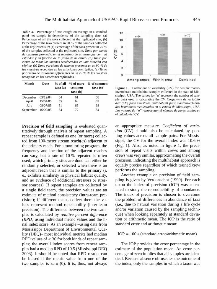
The Multihabitat Approach of USEPA’s Rapid Bioassessment Protocols 845
Table 3. Percentage of taxa caught on average in a standardpond net sample in dependence of the sampling date. (a)Percentage of all the taxa collected at the replicated site; (b)Percentage of the taxa present in 90 % of the samples collectedat the replicated site; (c) Percentage of the taxa present in 75 %of the samples collected at the replicated site. Tanto por cientode capturas promedio en el muestreo de un estanque con redestandar y en funcion de la fecha de muestreo. (a) Tanto porciento de todos los taxones recolectados en una estacion conreplica. (b) Tanto por ciento de taxones presentes en un 90 % delas muestras recogidas en las estaciones con replica. (c) Tantopor ciento de los taxones pfresentes en un 75 % de las nuestrasrecogidas en las estaciones replicadas.
Month Date % of all % of more % of commontaxa (a) common taxa (c)
taxa (b)
December 03/12/84 54 61 68April 15/04/85 55 63 67July 08/07/85 51 65 68
September 16/09/85 64 77 84
Precision of field sampling is evaluated quan-titatively through analysis of repeat sampling. Arepeat sample is defined as one (or more) collec-ted from 100-meter stream reach(es) adjacent tothe primary reach. For a monitoring program, thefrequency and location of the adjacent reachescan vary, but a rate of 10 % repeated is oftenused; which primary sites are done can either berandomly selected, or selected when there is anadjacent reach that is similar to the primary (i.e., exhibits similarity in physical habitat quality,and no evidence of additional stressors or stres-sor sources). If repeat samples are collected bya single field team, the precision values are anestimate of method consistency (intra-team pre-cision); if different teams collect them the va-lues represent method repeatability (inter-teamprecision). The difference between the two sam-ples is calculated by relative percent difference(RPD) using individual metric values and the fi-nal index score. As an example –using data fromMississippi Department of Environmental Qua-lity (DEQ)– most individual metrics had medianRPD values of < 30 for both kinds of repeat sam-ples; the overall index scores from repeat sam-ples had a median RPD of 10.5 (Mississippi DEQ2003). It should be noted that RPD results canbe biased if the metric value from one of thetwo samples is zero (0). It is, thus, not always
Figure 1. Coefficient of variability (CV) for benthic macro-invertebrate multihabitat samples collected in the state of Mis-sissippi, USA. The values for “n” represent the number of sam-ple pairs used in calculating the CV. Coeficiente de variabili-dad (CV) para muestreos multihabitat para macroinvertebra-dos bentonicos recolectadas en el estado de Mississippi, USA.Los valores de “n” representan el numero de pares usados enel calculo del CV.
an appropriate measure. Coefficient of varia-tion (CV) should also be calculated by poo-ling values across all sample pairs. For Missis-sippi, the CV for the overall index was 10.6 %(Fig. 1). Also, as noted in figure 1, the preci-sion of repeat visits within crews and amongcrews was very similar, approximating the overallprecision, indicating the multihabitat approach isequally precise regardless of which trained crewperforms the sampling.
Another example on precision of field sam-pling is given by Verdonschot (1990). For eachtaxon the index of precision (IOP) was calcu-lated to study the reproducibility of abundance.The index of precision is chosen to overcomethe problem of differences in abundance of taxa(i.e., due to natural variation during a life cycleand/or variation caused by the sampling techni-que) when looking separately at standard devia-tion or arithmetic mean. The IOP is the ratio ofstandard error and arithmetic mean:
IOP = 100 ∗ (standard error/arithmetic mean).
The IOP provides the error percentage in theestimate of the population mean. An error per-centage of zero implies that all samples are iden-tical. Because absence obfuscates the outcome ofthe index, only the samples in which a taxon was

846 Barbour et al.
Figure 2. The relation between the presence of the taxa andthe index of precision (IOP) calculated for observed abundan-ces. Relacion entre la presencia de taxones y el ındice de pre-cision (IOP) calculado para las abundancias observadas.
present were taken into account. The precision ofthe value of the abundance of a taxon can onlybe indicated for the moment it was collected. Fortaxa collected only once, the standard deviationand the index are indeterminate.
In figures 2 and 3, the IOP of a taxon is plottedagainst its frequency. For observed abundancesthe index fluctuates between 60 % and 200 %(Fig. 2). This means that if a taxon is collectedin one standard pond net sample, its abundanceestimate is not very precise.
To make the distribution of observed valuesless skew, the abundances are transformed to a lo-
Figure 3. The relation between the presence of the taxaand the index of precision (IOP) calculated for transfor-med abundances. Relacion entre la presencia de taxones y elındice de precision (IOP) calculados para las abundanciastransformadas.
garithmic scale. The index for transformed abun-dances fluctuates around 45 % (Fig. 3). Hence,this log transformation has been performed be-fore processing the data. Elliott (1971) reported20 % (on the original scale) as a reasonable errorin homogeneous bottom samples. The standardpond net samples were not taken from a homoge-neous substratum but from several microhabitats.Therefore, an index error of 45 % is consideredacceptable when the conditions are more or lessheterogeneous (patchy).
Question 3-What is the relative ability of themultihabitat method to distinguish natural va-riability (i.e., temporal, spatial) from humandisturbance?
The ability of this method to distinguish naturalvariability from human disturbance is enhancedby minimizing method error and by calibratingrelative to natural factors. Calibration of anybiological assessment protocol entails stratifica-tion of the annual time period (index period tominimize seasonal influences) and areal extent(site class to incorporate biogeographic patternsand other natural factors) to which the indexis applicable. Those sites exhibiting physical,chemical, and/or hydrologic stressor intensitiesof a predetermined level (or greater) make upthe analytical truth (or true value). Sensitivityis very closely related to accuracy and is alsoreflected by discrimination efficiency (DE). Theproportion of those sites correctly identified bythe biological index as impaired is its accuracy,and is quantified as discrimination efficiency(DE). The multihabitat proportional methodproduced a mean DE of 89 % in Maryland(across 2 bioregions) and 92 % in Mississippi(across 5 bioregions) (Fig. 4). Maryland’s Bent-hic Index of Biological Integrity (B-IBI) has aDE of 92 % for non-coastal plain streams, and88 % for coastal plain streams (Stribling et al.1998). The Mississippi Benthic Index of StreamQuality (M-BISQ) is stratified into 5 bioregionswith DEs of 90 % (Northwest, East, and West),100 % (Black Belt), and 89 % (Northeast).

The Multihabitat Approach of USEPA’s Rapid Bioassessment Protocols 847
Figure 4. Discrimination efficiencies (DE) for benthic multi-metric indexes calibrated for the USA states of Maryland andMississippi. Eficiencias de discriminacion (DE) para ındicesbentonicos multimetricos calibrados para los estados de Maty-land y Mississippi de USA.
Question 4-How would the multihabitatmethod be implemented forlow-gradient streams?
Development of a calibrated biological index, re-gardless of bioregion but specified for a stressor,has seven steps:
1. Identify candidate reference sites that repre-sent the suite of habitat types in low gradientstreams
2. To calibrate a biological index, sample alonga gradient of sites from natural background tostressed sites with the selected stressor.
3. Compile and calculate candidate metrics thatare ecologically relevant for low gradientstreams.
4. Test candidate metrics for distinguishing bet-ween reference and impaired sites.
5. Aggregate metrics into biological index that isscientifically robust to measure the stressors.
6. Test validity of index using an independentdataset
Step 1 is the more effort-intensive componentof this process. It includes selection of sites, sam-pling and processing of all field samples and data(biological, physical, and chemical), compilationof all ancillary data (e. g., land use), institutingappropriate and comprehensive quality assurance
and quality control (QA/QC), and population of aflexible data management system. The number ofstream sites necessary to adequately characterizeeach site class should be between 10-25, depen-ding on landscape heterogeneity (higher numberof sites for a more variable site class). Steps 2-6are described in detail in Barbour et al., (1999).
RECOMMENDATIONS
The multihabitat approach to sampling for bioas-sessment has been well tested in the USA and inEurope. The approach is used in comprehensivesurveys throughout broad jurisdictions. The pri-mary advantage is to afford a versatile method forsampling a wide variety of stream types, and isapplicable to evaluating both chemical and non-chemical stressors. Agencies and consortia inte-rested in a multihabitat approach should (i) iden-tify their program objectives that would be con-ducive to sampling representative aquatic habi-tats, (ii) characterize their aquatic systems suchthat the major stream types and associated habi-tats are described, (iii) agree upon a standard setof protocols for sampling the streams throughoutthe jurisdiction, and (iv) use only trained profes-sionals to ensure a high level of precision and re-presentativeness of the samples.
Legacy databases that have been populatedwith ecological data collected with otherapproaches should not be considered useless.The historical assessments conducted withthese data are still valid as benchmarks, andcross-calibration analyses could be done toreconcile varying assessments. It is likely thatafter cross-calibraton, only a few differences inresults will require substantiating a change inassessment of ecological condition.
REFERENCES
AQEM consortium. 2002. Manual for the applicationof the AQEM method. A comprehensive method toassess European streams using benthic macroinverte-brates, developed for the purpose of the Water Fra-mework Directive. Version 1.0, February 2002. 89 pp.

848 Barbour et al.
BARBOUR, M. T. 1997. The re-invention of biologi-cal assessment in the U.S. Human and EcologicalRisk Assessment, 3: 933-940.
BARBOUR, M. T., J. GERRITSEN, B. D. SNYDER& J. B. STRIBLING. 1999. Rapid BioassessmentProtocols for Use in Streams and Wadeable Rivers:Periphyton, Benthic Macroinvertebrates and Fish.Second Edition. EPA/841-B-99-002. U.S. EPA,Office of Water, Washington, D.C. 197 pp. plusappendices.
BARBOUR, M. T., J. GERRITSEN, G. E. GRIF-FITH, R. FRYDENBORG, E. MCCARRON, J. S.WHITE & M. L. BASTIAN. 1996. A frameworkfor biological criteria for Florida streams usingbenthic macroinvertebrates. J. North Am. Benthol.Soc., 15: 185-211.
DAVIS, W. S. & T. P. Simon (eds.).1995. Biologicalassessment and criteria: Tools for water resourceplanning and decision making. Lewis Publishers,Boca Raton, Florida. 415 pp.
DE LANGE, L. & M. A. DE RUITER.1977. Bio-logische Waterbeoordeling. Methoden voor hetbeoordelen van Nederlands oppervlaktewater opbiologische grondslag. Werkgroep BiologischeWaterbeoordeling. Instituut voor Milieuhygiene enGezondheidstechniek TNO, Delft. 251 pp.
ELLIOTT, J. M. & P.A. TULLETT. 1983. A bi-bliography of samplers for benthic invertebra-tes. Freshwater Biological Association, OccasionalPublication, 20. 1-26.
ELLIOTT, J. M. 1971. Some methods for the statis-tical analysis of samples of benthic invertebrates.Freshwat. Biol. Ass. Sc. Publ., 25. 248 pp.
ENVIRONMENT AGENCY. 1999. Procedures forcollecting and analysing macroinvertebrate samples.EnvironmentAgencyDocumentBT001.179pp.
FLORIDA DEPARTMENT OF ENVIRONMEN-TAL PROTECTION (FL DEP). 1996. Standardoperating procedures for biological assessment.Florida Department of Environmental Protection,Biology Section. July 1996. 98 pp.
FURSE M. T., J. F. WRIGHT, P. D. ARMITAGE& D. MOSS. 1981. An appraisal of pond-netsamples for biological monitoring of lotic macro-invertebrates. Wat. Res., 15: 679-689.
HERING, D., O. MOOG, L. SANDIN & P. F. M.VERDONSCHOT. 2004. Overview and applica-tion of the AQEM assessment system. Hydrobio-logia, 516: 1-20.
ISO 7828. 1985. Water quality –methods of biologi-cal sampling– guidance on handnet sampling of
aquatic benthic macro-invertebrates. Ref. No. ISO7828-1985 (E). 6 pp.
LENAT, D. R. 1988. Water quality assessment ofstreams using a qualitative collection method forbenthic macroinvertebrates. J. North Am. Benthol.Soc., 7: 222-233.
LENAT, D. R. 1990. Reducing variability in freshwa-ter macroinvertebrate data. In: Proceedings of the1990 Midwest Pollution Control Biologists Mee-ting. W. S. Davis (ed.).:1 9-32. U.S. EPA RegionV, Environmental Sciences Division, Chicago, IL.EPA-905-9-90/005.
LENAT, D. R. & M. T. BARBOUR. 1994. Usingbenthic macroinvertebrate community structure forrapid, cost-efficient, water quality monitoring: Ra-pid bioassessment. In: Biological Monitoring ofAquatic Systems. S. L. Loeb and A. Spacie (eds).:187-215. Lewis Publishers, Ann Arbor, Michigan.
LOEB, S. L. & A. SPACIE. 1994. Biological Monito-ring of Aquatic Systems. Lewis Publications, BocaRaton, Florida. 381 pp.
MAJOR, E. B. & M. T. BARBOUR. 2001. Standardoperating procedures for the Alaska Stream Con-dition Index: A modification of the U.S. EPA Ra-pid Bioassessment Protocols. 5th ed. Prepared forthe Alaska Department of Environmental Conser-vation. Environment and Natural Resources Insti-tute, University of Alaska Anchorage, Anchorage,AK. 1 vol. 52 pp.
MAJOR, E. B., M. T. BARBOUR, J. S. WHITE &L. S. HOUSTON. 1998. Development of a bio-logical assessment approach for Alaska streams:A pilot study on the Kenai Peninsula. Environ-ment and Natural Resources Institute, Universityof Alaska Anchorage, Anchorage, AK. Report forAlaska Department of Environmental Conserva-tion, Anchorage, AK. 31 pp. and appendix. 68 pp.
MASSACHUSETTS DEPARTMENT OF EN-VIRONMENTAL PROTECTION (MA DEP).1995. Massachusetts DEP preliminary biologicalmonitoring and assessment protocols for wadablerivers and streams. Massachusetts Departmentof Environmental Protection, North Grafton,Massachusetts. 121 pp.
MAXTED, J. R., M. T. BARBOUR, J. GERRIT-SEN, V. PORETTI, N. PRIMROSE, A. SILVIA,D. PENROSE & R. RENFROW. 2000. Assessmentframework for mid-Atlantic coastal plain streamsusing benthic macroinvertebrates. J. North Am.Benthol. Soc., 19: 128-144.

The Multihabitat Approach of USEPA’s Rapid Bioassessment Protocols 849
MID-ATLANTIC COASTAL STREAMS WORK-GROUP (MACS). 1996. Standard operating pro-cedures and technical basis: Macroinvertebratecollection and habitat assessment for low-gradientnontidal streams. Delaware Department of NaturalResources and Environmental Conservation, Do-ver, Delaware. 136 pp.
MINSHALL, G. W. 1984. Aquatic insect-substratumrelationships. In: The ecology of aquatic insects.V.H. Resh and D.M. Rosenberg (eds.): 358-400.Praeger Publishers, New York.
MISSISSIPPI DEPARTMENT OF ENVIRONMEN-TAL QUALITY (MDEQ). 2003. Development andApplication of the Mississippi Benthic Index ofStream Quality (MBISQ). June 30, 2003. Missis-sippi Department of Environmental Quality, Officeof Pollution Control, Jackson, MS. 82 pp. plus ap-pendices.
MOOG, O., A. CHOVANEC, J. HINTEREGGER& A. ROMER. 1999. Richtlinie zur Bestim-mung der saprobiologischen Gewassergute vonFließgewassern. Bundesministerium fur Land-undForstwirtschaft, Wien. 144 pp.
PLAFKIN, J. L., M. T. BARBOUR, K. D. PORTER,S. K. GROSS & R. M. HUGHES. 1989. Rapid bio-assessment protocols for use in streams and rivers:Benthic macroinvertebrates and fish. EPA/440/4-89/001. U.S. EPA Office of Water, Washington,DC. 128 pp. pluis appendices.
ROSENBERG, D. M. & V. H. RESH. 1993. Intro-duction to freshwater biomonitoring and benthicmacroinvertebrates. In: Freshwater biomonitoringand benthic macroinvertebrates. D. M. Rosenbergand V. H. Resh (eds.): 1-8. Chapman and Hall,New York.
SLADECEK, V. 1973. System of water quality fromthe biological point of view. Ergebnisse der Lim-nologie, 7: 1-128.
STRIBLING, J. B., B. K. JESSUP, J. S. WHITE, D.BOWARD & M. HURD. 1998. Development ofa Benthic Index of Biotic Integrity for MarylandStreams. Maryland Department of Natural Resour-ces. MANTA Report No. CBWP-EA-98-3. Anna-polis, MD. 36 pp.
VERDONSCHOT, P. F. M. 1990. Ecological cha-racterization of surface waters in the province ofOverijssel (The Netherlands). Thesis, Wagenin-gen, 255 pp.
WOODIWISS, F. S. 1978. Comparative study ofbiological-ecological water quality assessmentmethods. Summary report, Commission of the Eu-ropean Communities. Nottingham, Sept/Oct. 1976.231 pp.
WRIGHT, J. F., D. W. SUTCLIFFE & M. T. FURSE(eds.). 2000. Assessing the biological quality offresh waters – RIVPACS and other techniques.Freshwater Biological Association, Ambleside,Cumbria, UK, 373 pp.
