Revista Român! de Statistic!

Supliment

Romanian Statistical Review Supplement

2/2017

Institutul Na�ional de Statistic�

National Institute of Statistics

www.revistadestatistic .ro/supliment

COLEGIUL !TIIN"IFIC

EMILIAN DOBRESCU - academician, Academia Român!

AUREL IANCU - academician, Academia Român!

MARIUS IOSIFESCU - academician, Academia Român!

LUCIAN ALBU - academician, Academia Român!

GHEORGHE ZAMAN � Prof. univ. dr., membru corespondent al Academiei Române

TUDOREL ANDREI - Prof. univ. dr., Academia de Studii Economice

DAN GHERGU" - Lect. univ. dr. , Universitatea Titu Maiorescu, Bucure"ti

KONRAD PASENDORFER � PhD, Director General al Statistics Austria

MARIANA MIHAILOVA KOTZEVA - EUROSTAT

CONSTANTIN MITRU" � Prof. univ. dr., Pre"edinte al Societ!#ii Române de Statistic!

CONSTANTIN ANGHELACHE � Prof. univ. dr., Vicepre"edinte al Societ!#ii Române de Statistic!

NICOLAE ISTUDOR � Prof. univ. dr., Rector al Academiei de Studii Economice, Bucure"ti

VERGIL VOINEAGU � Prof. univ. dr., Academia de Studii Economice, Bucure"ti

TIBERIU POSTELNICU � Prof. univ. dr., Institutul �Gheorghe Mihoc-Caius Iacob�

BOGDAN OANCEA � Prof. univ. dr., Universitatea Bucure"ti

GHEORGHE S#VOIU - Conf. univ. dr., Universitatea Pite"ti

IRINA-VIRGINIA DRAGULANESCU - Prof. univ. dr., University Messina, Italia

DANIELA ELENA !TEF#NESCU - Conf. univ. dr., Institutul Na#ional de Statistic!

ELISABETA JABA � Prof. univ. dr., Universitatea �Alexandru Ioan Cuza� University

EUGENIA HARJA - Prof. univ. dr., Universitatea Vasile Alecsandri, Bac!u

!TEFAN-ALEXANDRU IONESCU - Lect. univ. dr. Universitatea Româno-American!

CLAUDIU HER"ELIU - Prof. univ. dr., Academia de Studii Economice

ION GHIZDEANU - Dr., cercet!tor "tiin#i$ c gradul I, Comisia Na#ional! de Prognoz!

ILIE DUMITRESCU - Institutul Na#ional de Statistic!

SILVIA PISIC# - Dr., Institutul Na#ional de Statistic!

ADRIANA CIUCHEA - Institutul Na#ional de Statistic!

Revista Română de Statistică - Supliment nr. 2 / 2017

SUMAR / CONTENTS 2/2017REVISTA ROMÂNĂ DE STATISTICĂ SUPLIMENT

ASPECTE SEMNIFICATIVE PRIVIND CONSUMUL ŞI ECONOMISIREA 3SIGNIFICANT ISSUES ON CONSUMPTION AND SAVING 12Prof. univ. dr. Alexandru MANOLEConf. univ. dr. Madalina-Gabriela ANGHELDrd. Georgiana NIȚU

PRECAUŢIUNEA ECONOMISIRII ÎN CONDIŢII DE INCERTITUDINE 21PRECAUTION OF SAVINGS UNDER UNCERTAIN CIRCUMSTANCES 30Prof. univ. dr. Constantin ANGHELACHEConf. Univ. Dr. Aurelian DIACONU Drd. Emilia STANCIU

ELEMENTE TEORETICE PRIVIND MANAGEMENTUL DE PORTOFOLIU DINAMIC 38THEORETICAL ASPECTS OF THE DYNAMIC PORTFOLIO MANAGEMENT 47Conf. univ. dr. Madalina-Gabriela ANGHELConf. univ. dr. Mirela PANAITProf. univ. dr. Alexandru MANOLEDrd. Marius POPOVICI

DIVERSIFICAREA TEMPORALĂ ÎN CONSUM ŞI ECONOMISIRE 56TIME DIVERSIFICATION IN CONSUMPTION AND SAVING 64Prof. univ. dr. Constantin ANGHELACHEProf. univ. dr. Radu Titus MARINESCU Asistent univ dr. Diana Valentina DUMITRESCU

MODEL DE ANALIZĂ A CORELAŢIEI DINTRE PRODUSUL INTERN BRUT ŞI COMPONENTELE CONSUMULUI FINAL 71MODEL ANALYSIS OF THE CORRELATION BETWEEN GDP AND FINAL CONSUMPTION COMPONENTS 84Prof. univ. dr. Constantin ANGHELACHEDrd. Andreea Ioana MARINESCUDrd. Doina AVRAMDrd. Doina BUREADrd. Gyorgy BODO

MODEL DE ANALIZĂ A CORELAŢIEI DINTRE CONSUMUL FINAL ŞI COMPONENTELE ACESTUIA 96MODEL ANALYSIS OF THE CORRELATION BETWEEN FINAL CONSUMPTION AND ITS COMPONENTS 105Prof. univ. dr. Alexandru MANOLE Lector univ. dr. Mariana BUNEA Lector univ. dr. Ana CARPAsist. Univ. Dr. Diana-Valentina SOAREDrd. Maria MIREA

www.revistadestatistica.ro/supliment

Romanian Statistical Review - Supplement nr. 2 / 20172

MODEL ECONOMETRIC DE ANALIZĂ A CORELAŢIEI DINTRE PRODUSUL INTERN BRUT ŞI CONSUMUL FINAL 114ANALYSIS OF THE ECONOMETRIC MODEL OF THE CORRELATION BETWEEN GDP AND FINAL CONSUMPTION 122Conf. univ. dr. Mădălina-Gabriela ANGHELDrd. Radu STOICADrd. Tudor SAMSONDrd. Alexandru BADIU

THE CONTRIBUTION OF HIGHER EDUCATION TO THE ACCUMULATION OF HUMAN CAPITAL IN THE ROMANIAN ARCHITECTURE FIELD DURING COMMUNISM 130Valentin Maier

METHODOLOGICAL AND APPLICATIVE PROBLEMS OF USING PEARSON CORRELATION COEFFICIENT IN THE ANALYSIS OF SOCIO-ECONOMIC VARIABLES 148Daniela-Emanuela Dănăcică

THE INFLUENCE OF THE MARKETING COMMUNICATION ON CONSUMER BEHAVIOR 164Gheorghe ORZANRaluca-Florentina TIŢA Raluca-Giorgiana CHIVU Ștefan-Ilie OANȚĂ Cristian Ionuț COMAN

Revista Română de Statistică - Supliment nr. 2 / 2017 3

Aspecte semnifi cative privind consumul şi economisirea

Prof. univ. dr. Alexandru MANOLEUniversitatea „ARTIFEX” din BucureștiConf. univ. dr. Madalina-Gabriela ANGHELUniversitatea „ARTIFEX” din BucureștiDrd. Georgiana NIȚU

Academia de Studii Economice din București

Abstract

In acest articol, autorii analizează unele aspecte privind corelaţia dintre consum şi economisire. Sunt abordate consumul şi economisirea în condiţii certe, fl uctuaţia în timp a consumului, posibilităţile de creştere a consumului în mod optim în condiţii de certitudine. Modelele prezentate sunt descrise în detaliu şi comentate. Între economisire și consum se derulează întreaga dinamică subiectivă a comportamentului uman care pendulează între achiziționare de bunuri și hârtii de valoare și păstrarea într-o formă sau alta a banilor. Într-o formă sau alta, pentru că achiziția de titluri de valoare sau acțiuni, dincolo de caracterul comercial al acțiunii, semnifi că totuși o investiție în hârtii cu valoare corespunzătoare banilor, care, în fi nal, reprezintă și ei hârtii investite cu o anumită valoare și, inevitabil, și semnifi cație. Aceste două ipostaze ale dinamicii decidentului fac parte din elementele arcului de timp important important în modelarea comportamentului subiectiv al decidentului. Scoțând inițial actul de modelare în afara timpului, prin considerarea demersului decizional ca derulat într-o singură perioadă de timp, s-au stabilit regulile modelării matematice a comportamentului decizional într-un cadru static, supus doar acțiunii unui anumit număr de variabile, afl ate cât mai puțin sub imperiul subiectivității și cât mai mult sub cel al obictivității. Cuvinte cheie : certitudine, decizie, consum, economisire, resurse Clasifi care JEL : E20, E21

Introducere

Până acum, am asumat faptul de decidentul acoperă doar un singur ciclu. Aceasta perspectivă obscurizează dimensiunea intertemporală importantă a riscului. În viața reală, agenții pot amâna riscul pentru mai târziu. Într-adevăr, abilitatea de a amâna alegerile riscante crește valoarea propriei

Romanian Statistical Review - Supplement nr. 2 / 20174

alegeri, de obicei numită ”valoare alegerii reale”. Decidenții pot alege să împartă câștigurile și pierderile posibile în alegerile curente pe care le au de făcut în mai multe perioade de timp și cicluri, care devine astfel un tip de diversifi care temporală a efectelor riscului cu privire la consumul fi nal. Alternativ, ei pot spera să recupereze unele dintre pierderile curente asumându-și riscuri suplimentare în viitor. În extrem, acest tip poate conduce la strategia ”asumă-ți pierderea totală”, precum un jucător la Las Vegas care pariază puținii bani de care dispune într-un pariu fi nal și ultim în speranța de a recupera pierderile masive suferite. În fi nal, agenții pot schimba nivelele de consum și economisire planifi cate în așteptarea confruntării viitoare cu incertitudinea, precum și să economisească un pic mai mult în fazele anterioare ca un gen de protecție față de riscuri viitoare. Vom analiza în continuare relația dintre risc și timp. Ne vom concentra pentru mment pe impactul riscului asupra organizării judicioase a consumului și economisirii.

Literature review Înțelegerea comportamentului de consum este probabil una dintre cele mai importante provocări ale macroeconomiei moderne. În acest domeniu s-au înregistrat abordări nenumărate începând cu lucrările lui Modigliani și Brumberg(1954) și Friedman(1957). Aceste dezvoltări se referă la teoria ciclurilor reale de afaceri. Estimările relative la gradul de rezistență la fl uctuațiile consumului pot fi menționate în diferite lucrări. Hall(1988) a menționat o estimare în jurul valorii 10, în timp ce Epstein și Zin (1991) au descoperit valori cuprinse între 1,25 și 5. Un experiment în acest sens a fost realizat de Barsky, Juster, Kimball și Shapiro(1997). Prima analiza formală a economisirilor precuate este datorată lui Leland(1968), Sandmo(1970) și Dreze și Modigliani(1972). Kimball (1990) a fasonat termenul de prudență examinând proprietățile primei de precauție. De-a lungul timpului s-a consolidat o literatură importantă asupra efectului limitărilor de lichiditate în cadrul ratelor optime de economisire. Strotz (1956) a fost primul care a pus în discuție problema consistenței temporale în cazul consumatorilor care folosesc un factor de reducere care nu descrește exponențial cu orizontul de timp. Pollack (1968) a rezolvat problema consistenței temporale utilizând o abordare din teoria jocurilor în care diferiți jucători reprezintă sivariante diferite ale aceluiasi consumator în perioade de timp diferite. Laibson (1997) reexaminează această chestiune pentru a explica diferite aspecte ale piețelor de credit astfel că avem astăzi o vastă literatură asupra “reducerii hiperbolice”. Anghelache şi Anghel (2016, 2014) prezintă instrumentele econometrice utile în analize la nivel micro şi macroeconomic şi instrumentele modelării economico-fi nanciare. Anghelache (2008)este o lucrare de referinţă

Revista Română de Statistică - Supliment nr. 2 / 2017 5

în statistica economică. Anghelache, Anghelache şi Sacală (2016) analizează evoluţia investiţiilor de capital în România. Anghelache, Manole şi Anghel (2015) studiază, prin regresie unifactorială, caracteristicile consumului fi nal, Anghelache, Manole şi Anghel (2015) analizează efectul dinamicii consumului fi nal şi investiţiilor asupra Produsului Intern Brut al României. Anghelache, Manole şi Dumitrescu (2015) evaluează corelaţiile dintre consumul fi nal, venitul brut disponibil şi investiţii.

Metodologie şi date

1. Consumul și economisirea în condiții certe

Ca reper cazuistic, vom porni cu caracterizarea consumului optim în condiții de certitudine Să presupunem că un agent decident trăiește pentru un număr cunoscut de cicluri. Denotăm timpul prin indexarea n a datei t = 0,…n - 1. Agentul dispune de un fl ux fi nanciar sigur yt, unde yt denotă încasări sigure la data t. Se presupune existența unei pieți de credit efi ciente cu rată constantă lipsită derisc r atât pentru credit, cât și pentru împrumut. În fi ecare ciclu, agentul decide cât de mult va consuma, ceea ce va defi ni implicit cât de mult va cheltui sau cât va economisi. Dacă ct denotă consumul la data t, condiționarea dinamică a bugetului poate fi exprimată astfel:

zt+1 = (1 + r)[zt + yt ct], t =0,…,n – 1, (1) unde zt reprezintă suma transferată din data t – 1 la data t. Presupunem că suma inițială z0 este zero.

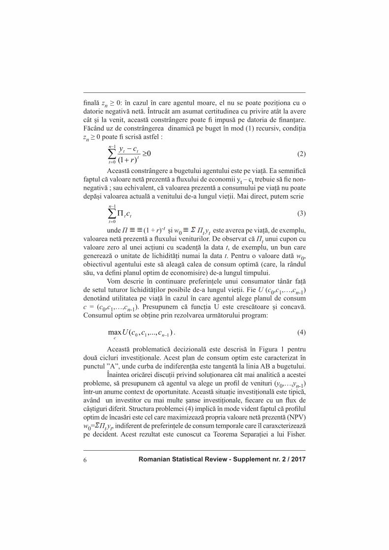
Figura 1

Întrucât împrumutătorii nu vor accepta să acorde credit agenților care nu vor fi în stare să restituie datoria mai târziu, se formulează o constrângere

Romanian Statistical Review - Supplement nr. 2 / 20176

fi nală zn ≥ 0: în cazul în care agentul moare, el nu se poate poziționa cu o datorie negativă netă. Întrucât am asumat certitudinea cu privire atât la avere cât și la venit, această constrângere poate fi impusă pe datoria de fi nanțare. Făcând uz de constrângerea dinamică pe buget în mod (1) recursiv, condiția zn ≥ 0 poate fi scrisă astfel :

0

)1(

1

0∑−

=

≥+

−n

tttt

r

cy (2)

Această constrângere a bugetului agentului este pe viață. Ea semnifi că faptul că valoare netă prezentă a fl uxului de economii yt – ct trebuie să fi e non-negativă ; sau echivalent, că valoarea prezentă a consumului pe viață nu poate depăși valoarea actuală a venitului de-a lungul vieții. Mai direct, putem scrie

∑−

=

Π1

0

n

ttt c

(3)

unde П (1 + r)-t și w0 Пt yt este averea pe viață, de exemplu, valoarea netă prezentă a fl uxului veniturilor. De observat că Пt unui cupon cu valoare zero al unei acțiuni cu scadență la data t, de exemplu, un bun care generează o unitate de lichidități numai la data t. Pentru o valoare dată w0, obiectivul agentului este să aleagă calea de consum optimă (care, la rândul său, va defi ni planul optim de economisire) de-a lungul timpului. Vom descrie în continuare preferințele unui consumator tânăr față de setul tuturor lichidităților posibile de-a lungul vieții. Fie U (c0,c1,…,cn-1) denotând utilitatea pe viață în cazul în care agentul alege planul de consum c = (c0,c1,…,cn-1). Presupunem că funcția U este crescătoare și concavă. Consumul optim se obține prin rezolvarea următorului program:

),...,,(max 110 −n

ccccU . (4)

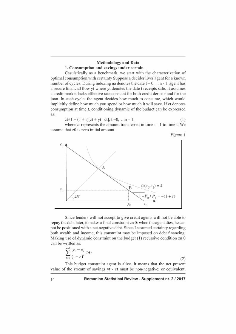
Această problematică decizională este descrisă în Figura 1 pentru două cicluri investiționale. Acest plan de consum optim este caracterizat în punctul ”A”, unde curba de indiferențăa este tangentă la linia AB a bugetului. Înaintea oricărei discuții privind soluționarea cât mai analitică a acestei probleme, să presupunem că agentul va alege un profi l de venituri (y0,…,yn-1) într-un anume context de oportunitate. Această situație investițională este tipică, având un investitor cu mai multe șanse investiționale, fi ecare cu un fl ux de câștiguri diferit. Structura problemei (4) implică în mode vident faptul că profi lul optim de încasări este cel care maximizează propria valoare netă prezentă (NPV) w0= Пt yt, indiferent de preferințele de consum temporale care îl caraxcterizează pe decident. Acest rezultat este cunoscut ca Teorema Separației a lui Fisher.

Revista Română de Statistică - Supliment nr. 2 / 2017 7

Aceasta susține regula NPV, care este una dintre cele mai importante reguli din ștințele economice : Orice investitor ar trebui să aleagă o investiție care maximizează valoare netă prezentă ΣПt (1 + r)-t a fl uxului fi nanciar. Problema (4) nu este prea diferită de problema deciziei statice a unui agent care consumă n bunuri fi zice într-o teorie clasică a cererii. Proprietățile generale ale acestor funcții sunt binecunoscute. Modelul poate fi îmbogățit cu o propunere legată de preferințele temporale, respectiv introducerea unei axiome care asumă că ordinul preferinței deasupra perechii (c0, c1) nu depinde de modalitatea de consum pentru cele două cicluri n-2, adică, dacă (a,b,c2, …,cn-

1) este preferat lui (d, e,c2, … , cn-1), atunci (a, b, x2, … , xn-1) este preferat lui (d, e, x2, … , xn-1) pentru toți (x2, …, xn-1). Aceasta exclude fenomene precum formarea obiceiurilor de consum. Această presupunere de independență implică faptul că utilitatea funcției U trebuie să fi e separabil, U(c) t (ct), unde ut este utilitatea (intraperioadă) a consumului în momentul t. Pentru a distinge între funcția de utilitate intertemporală U, pe care o numim ut ca ”funcție a fericirii” a consumului la momentul t. O presupunere comună este aceea că funcțiile de fericire sunt echivalente: ut(·)= pt u(·), pentru unele funcții crescătoare și concave u și pentru un scalar pt > 0. Cei mai mulți cercetători au adoptat acest set de presupuneri în ultimii 50 de ani. Păstrând caracterul de generalitate, considerăm p0 ca unitate. Astfel p poate fi interpretat ca o reducere a factorului de fericire u(ct) la momentul t. Dacă pt este mai mic decât unitatea, poate fi interpretat ca pierdere proporțională a utilității cauzată de amânarea consumului, de exemplu, acesta indică o preferință pentru a consuma mai devreme decât mai târziu. Este important să disociem pt, un parametru psihologic, de r, o variabilă fi nanciară. Parametrul pt este folosit ca factor de reducere a fericirii, în timpp ce rata dobânzii r este utilă doar în reducerea fl uxurilor monetare, așa cum s-a văzut anterior. Folosind aceste restricții, putem rescrie problema consumului astfel:

∑−

=

1

0

)(maxn

ttt

ccup subject to 0

1

0

ω=Π∑−

=

n

ttt c

(5)

Condițiile de prim ordin pentru această problem pot fi scrise ca ptu̕ (ct) = ξ Пt pentru t = 0, … n-1 (6) laolaltă cu restrângerea bugetului, unde ξ este multiplicatorul Lagrange asociat cu problema (6.5). Multiplicatorul Lagrage ξ este pur și simplu utilitatea marginal pe viață a unei creșteri a valorii actuale a bunăstării. Această problemă este formal echivalentă cu problema portofoliului static Arrow-Debreu. Înlocuim doar ”stări de natură” cu date, probabilități cu factori de reducere, și ”titluri de valoare” Arrow-Debreu cu cupoane – obligațiuni cu valoare zero. Echivalența are numeroase consecințe pentru ipotezele de lucru.

Romanian Statistical Review - Supplement nr. 2 / 20178

2. Consideraţii privind fl uctuațiile consumului în timp

În primul rând, putem interpreta concavitatea funcției de fericire u în contextul problemei consum-economisire într-o anumită perioadă de timp. Faptul că utilitatea marginală este descrescătoare cu privire la consum generează stimulente pentru decident în sensul unui consum constant în timp. Să considerăm cazul special unde pt = 1 pentru toți t, și cu r = 0, ceea ce implică Пt = 1 pentru toți t. Din condițiile de prim-ordin (6.6) rezultă că u̕ (ct) = ξ pentru fi ecare perioadă, astfel încât calea consumului optim nu manifestă nicio fl uctuație în consum de la o perioadă la alta : ct = w0/n pentru toate valorile lui t. Aceasta este o împrejurare canâplanul de consum optim A este într-o linie de 45° în Figura 6.1.Dacă veniturile fl uctuează de-a lungul vieții consumatorului, strategia optimă de economisire constă în a economisi orice venit suplimentar peste w0/n, sau să împrumute bani în cazurile în care câștigurile din ciclu sunt mai mici decât w0/n. Concavitatea lui u implică faptul că condițiile de ordin secund sunt satisfăcute, astfel că utilitatea de-a lungul întregii vieți este maximizată prin consumul unei cantități egale în fi ecare perioadă. Astfel, dacă u ar fi convex, această soluție ar genera o utilitate minimă pe viață și este ușor de arătat că utilitatea maximă este realizată prin consumul dintr-un singur ciclu investițional. Concluzionăm că atunci când nu există nerăbdare (pt = 1), și rata dobânzii este zero (r = 0), fi ind situația optimă când poți uniformiza consumul dacă funcția de fericire este concavă. Astfel, presupunerea u̕ ̕ < 0 exprimă o aversiune față de fl uctuațiile consumului de-a lungul ”stărilor naturale” din problema portofoliului static Arrow-Debreu. În ultimul model, acesta implică faptul că asigurarea completă este optimă când prețurile bunurilor egalează probabilitatea fi ecărei stări. Se poate măsura intensitatea dorinței de a uniformiza consumul în timp considerând situația în care nu există o piață de credite, astfel că ct = yt. Să presupunem că venitul y0 la momentul 0 este strict mai mic decât venitul y1 la momentul 1. Întrucât utilitatea marginală a consumului este mai mare la termenul 0 decât la momentul 1, u̕ (y0) 1), știm că agentul nu va dori să schimbe o unitate de consum de astăzi pe o unitate de consum de mâine. Acordul privind un asemena model de înțeleger, ar duce la creșterea diferenței dintre consumul la moment 0 și momentul 1, și i-ar reduce utilitatea generală. Interogat în legătură cu sacrifi carea unei unități de consum în acest moment, agentul decident va cere mâine mai mult decât o unitate de consum pentru ziua următoare în calitate de compensație. O modalitate de a măsura intensitatea acestei rezistențe pentru a negocia consumul actual pentru consumul următor constă în defi nirea unei compensații suplimentare k > 0, consum care ar trebui acordat agentului la momentul 1 cu scopul de a micșora pierderea în consum la momentul zero. Considerând pierderile în consum ca fi ind sufi cient de mici, k este defi nit astfel

Revista Română de Statistică - Supliment nr. 2 / 2017 9

u̕(y0) = (1 + k)u̕ ( y1). Partea stânga a acestei egalități reprezintă costul marginal al reducerii consumului astăzi, în timp ce partea dreaptă reprezintă benefi ciul marginal al creșterii viitoare a consumului prin factorul 1 + k. Altfel spus, k poate fi defi nit astfel încât pierderea de utilitate marginalăprin renunțarea la o unitate de consum la momentul 0 trebuie să egaleze creșterea marginală a utilității prin adăugarea lui 1+k unități de consum la momentul 1.Dacă y1 este apropiat de y0,am putea folosi expansiunea Taylor de prim-ordin u̕ (y0) apropiată de y1 pentru a obține

−−≅

)('

)(''

1

11

1

01

yu

yuy

y

yyk

(7).

Rezistența față de substituirea intertemporală este aproximativ proporțională cu rata de creștere a consumului. Factorul de multiplicare, (y) = -yu̕̕ ̕(y)/u̕(y) mai este numit și măsura aversiunii față de fl uctuația relativă, sau grad relativ de rezistență la substituirea intertemporală a consumului. Evident,

(y) este similare cu măsura aversiunii relative față de risc a modelului Arrow –Pratt. Ambele evaluează descreșterea procentului utilității marginale privitoare la o minoră creștere procentuală a bunăstării, respectiv a consumului. În mod curent, o putem considera o măsură locală a aversiunii consumatorului față de amânarea consumului de la o dată sau moment cu consum scăzut către una cu consum ușor mărit. În acest sens, trebuie acordată o atenție mai mare estimărilor empirice ale lui (y), considerat undeva între 1 și 5.

3. Consumul în condiții de certitudine – sporirea optimă

În principiu, rata reală a dobânzii nu este zero, ceea ce alimentează neliniștea agenților decidenți. Să presupunem că consumatorii fac apel la principiu de discount exponențial, p1 =

t, pentru scalarul mai mic decât 1. Aceasta presupune un randament al ratei preferinței pure la momentul prezent de

(1 / pozitiv ca valoare. Altfel spus, -1 și rata fericirii u(ct) multiplicată cu t este echivalent cu scăderea fericirii la o rată constantă pentru perioada de timp respectivă. Utilizarea unei rate constante a reducerilor ulterioare ale utilităților este importantă pentru deciziile consumatorului privind consistența temporală, așa cum se va vedea în continuare. Nerăbdarea și un profi t pozitiv în economisire are două rațiuni echilibrante astfel încât să nu se uniformizeze consumul de-a lungul timpului. Un nivel înalt de nerăbdare, sau un mai înalt, provoacă agenților nevoia de a consuma mai devreme ca timp. Cu alte cuvinte, nerăbdarea tinde să pună la îndoială preferințele în favoarea căilor de consum care descresc în timp. Aceste două efecte contradictorii trebuie combinate cu aversiunea față de

Romanian Statistical Review - Supplement nr. 2 / 201710

fl uctuațiile consumului, în scopul obținerii unei caracterizări optime a creșterii consumului în condiții de siguranță. Exemplifi căm rezolvând analitic această problemă în cazul special în care funcția de fericire prezintă un grad relativ constant de aversiune față de fl uctuațiile consumului. Folosind analogia cu modelul Arrow-Debreu, obținem soluția ct = c0 a

t (8) unde

γ

δ

/1

1

1

++

=r

a

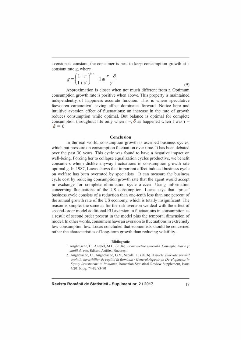
iar c0 este un consum inițial ales pentru a satisface constrângeri ale bugetului la nivelul întregii vieți. Astfel, când reducerea psihologică este exponențială, iar aversiunea relativă este constantă, pentru consumator este cel mai bine să mențină creșterea consumului la o rată constant g, unde

γδ

δ

γ−

≅−

++

≡rr

g 11

1/1

(9)

Aproximarea este mai apropiată când nu diferă prea mult de r. Rata de creștere optimă a consumului este pozitivă atunci când este mai mare decât . Această proprietate se menține independent de precizarea funcției de fericire. Acesta este cazul în caremotivul speculativ în facvoarea economisirii domină efectul de nerăbdare. Observă aici și efectul intuitiv al aversiunii față de fl uctuații : o creștere a lui reduce rata creșterii optime a consumului în timp. Dar, este optim Pentru echilibrarea completă a consumului de-a lungul întregii vieți numai atunci când r= , așa cum s-a întâmplat atunci când am avut r = .

Concluzii

În lumea reală, creșterea consumului este arondată ciclurilor de afaceri, care pun presiune pe fl uctuația consumului în timp. Acesta a fost subiect de dezbatere în ultimii 30 ani. Acest ciclu s-a dovedit a avea impact negativ asupra bunăstării. Obligând-o să se restrângă, prin egalizarea ciclurilor productive, am avantaja consumatorul căruia îi displac oricum fl uctuațiile consumului de la rata de creștere optimă g. In 1987, Lucas arata ca importanta efectului indus de ciclul de afaceri asupra bunastarii a fost mult supraevaluata de specialisti. Se poate masura costul ciclului de afaceri prin reducerea ratei de crestere a consumului pe care reprezentantul agentului ar accepta-o in schimbul eliminarii complete a ciclului de afeceri. Utilizand informatiile privitoare la fl uctuatiile consumului din SUA, Lucas arata ca ”pretul” ciclurilor de afaceri consta intr-o reducere cu mult mai putin decat o zecime dintr-un procent al ratei de crestere anuala a economiei SUA, ceea ce este total nesemnifi cativ.

Revista Română de Statistică - Supliment nr. 2 / 2017 11

Motivul este simplu : la fel ca si in cazul aversiunii fata de risc avem de a face cu un efect de ordin secund al modelului aditional EU, aversiunea fata de fl uctuatiile consumului fi ind un efect de ordin secund prezent in modelul care

se adauga in dimensiunea temporala a modelului. Cu alte cuvinte consumatorii

au o aversiune extrem de scazuta fata de fl uctuatiile mici ale consumului.

Lucas concluziona ca economistii ar trebui sa se preocupe, mai degraba, de

caracteristicile cresterii pe termen lung decat de reducerea volatilitatii.

Bibliografi e

1. Anghelache, C., Anghel, M.G. (2016). Econometrie generală. Concepte, teorie şi

studii de caz, Editura Artifex, Bucureşti

2. Anghelache, C., Anghelache, G.V., Sacală, C. (2016). Aspecte generale privind

evoluţia investiţiilor de capital în România / General Aspects on Developments in

Equity Investments in Romania, Romanian Statistical Review Supplement, Issue

4/2016, pg. 74-82/83-90

3. Anghelache, C., Manole, A., Anghel, M.G. (2015). Unifactorial Econometric

Model - Connection between the Final Consumption and the Private Consumption,

Asian Academic Research Journal Of Social Science & Humanities, Volume 2,

Issue 6, November 2015, pp. 212-219

4. Anghelache, C., Manole, A., Dumitrescu, D. (2015). The Correlation between Final

Consumption, Gross Available Income and Gross Investment: An Econometric

Analysis, International Journal of Academic Research in Accounting, Finance and

Management Sciences, Volume 5, No. 4, October 2015, pp. 84-88

5. Anghelache, C., Manole, A., Anghel, M.G. (2015). Analysis of fi nal consumption

and gross investment infl uence on GDP – multiple linear regression model,

Theoretical and Applied Economics, No. 3/2015 (604), Autumn, pg 137-142

6. Anghelache, C., Anghel, M.G. (2014). Modelare economică. Concepte, teorie şi

studii de caz, Editura Economică, Bucureşti

7. Anghelache, C. (2008). Tratat de statistică teoretică şi economică, Editura

Economică, Bucureşti

8. Cummins, J., Hassett, K., Oliner, S. (2006). Investment Behavior, Observable

Expectations, and Internal Funds, American Economic Review 96, no. 3, pp. 796-810

9. Deaton, A. (1991). Saving and liquidity constraints, Econometrica, 59

10. Dornbusch, R., Fischer, S., Startz, R. (2007). Macroeconomie - traducere, Editura

Economică, Bucureşti

11. Epstei, L.G., Zin, S.. (1991). Substitution, risk aversion and temporal behaviour

of consumption and assets returns: an empirical framework, Journal of political

economy, 99

12. Greenwood, R., Shleifer, A. (2014). Expectations of Returns and Expected

Returns, Review of Financial Studies 27, no. 3, pg. 714-746

13. Kimball, M.S. (1990). Precautionary cavings in the small and in the large,

Econometrica 58

14. Rampini, A.A., Viswanathan, S. (2010). Collateral, risk management, and the

distribution of debt capacity, Journal of Finance 65, 2293–2322

Romanian Statistical Review - Supplement nr. 2 / 201712

SIGNIFICANT ISSUES ON CONSUMPTION AND SAVING

Prof. Alexandru MANOLE PhD.

„ARTIFEX” University of BucharestAssoc. prof. Madalina-Gabriela ANGHEL PhD.

„ARTIFEX” University of BucharestGeorgiana NIȚU PhD. Student

Bucharest University of Economic Studies

Abstract

In this article, the authors analyze some aspects of correlation between consumption and savings. Consumption and savings are addressed to certain conditions, fl uctuation in time of consumption, the possibilities of increasing

consumption in optimally with certainty. The models presented are described

in detail and commented.

Between saving and consumption whole dynamic menus subjective

human behavior that oscillates between purchasing goods and securities

and preservation in some form of money. In one form or another, for the

acquisition of securities or shares, beyond the commercial character of the

action, signifi es still investing in securities with appropriate amount of money,

which ultimately represents her papers invested with a certain value and

inevitably and signifi cance.

These two aspects of the dynamics of decision-makers form part of

the spring while important in shaping behavior subjective decision-maker.

Removing the initial act of modeling out of time, by considering the approach

decision to run a single time, they set the rules of mathematical modeling

behavior decision in a static framework, subject only action of a number of

variables, which are as less under the sway of subjectivity and as much below

the obictivităţii.

Keywords: certainty, decision, consumption, saving resources JEL Classifi cation: E20, E21

Introduction

Until now, we assumed that the decision maker only covers one cycle. This perspective obscures important intertemporal dimension of risk. In real life, agencies can postpone the risk for later. Indeed, the ability to defer risky choices increase the value of their own choosing, usually called “value real choice.” Policy makers can choose to share the possible gains and losses in the current elections that we have done several times and cycles, which becomes

Revista Română de Statistică - Supliment nr. 2 / 2017 13

a kind of temporal diversifi cation of risk effects on fi nal consumption.

Alternatively, they can hope to recover some of the losses current assuming

additional risks in the future. In the extreme, this strategy can lead to “assume

your total loss”, as a player from Las Vegas to bet the little money available in

a fi nal and ultimate bet, hoping to recoup the massive losses suffered. Finally,

agencies can change levels of consumption and saving pending planned future

confrontation with uncertainty and to save a little more in the earlier phases

as a kind of protection against future risks. We will continue to analyze the

relationship between risk and time. Mment we will focus on the impact of risk

on the organization judicious consumption and saving.

Literature review

Understanding consumer behavior is probably one of the most

important challenges of modern macroeconomics. In this area there have been

numerous approaches from the works of Modigliani and Brumberg (1954)

and Friedman (1957). These developments relate to real business cycle theory.

Estimates relating to the degree of resistance to fl uctuations in consumption can

be mentioned in various papers. Hall (1988) mentioned an estimate around 10,

while Epstein and Zin (1991) found values between 1.25 and 5. An experiment

in this regard was made by Barsky, Juster, Kimball and Shapiro ( 1997). Precu

fi rst formal analysis of savings is due to Leland (1968), Sandmo (1970) and

Drez and Modigliani (1972). Kimball (1990) examining fashioned term care

premium properties caution. Over time it has consolidated a signifi cant literature

on the effect of liquidity constraints in the optimal rates of saving. Strotz (1956)

was the fi rst to put the issue of temporal consistency for consumers using a

discount factor that decreases exponentially with time horizon. Pollack (1968)

solved the problem using a temporal consistency from game theory approach in

which different players of the same consumer is different sivariante in different

periods. Laibson (1997) review this issue to explain different aspects of the credit

markets so that we have today is a vast literature on “reducing hyperbolic”.

Anghelache and Anghel (2016, 2014) presents econometric tools

useful in micro and macro level analyzes and modeling economic and

fi nancial instruments. Anghelache (2008) is a work of reference in economic

statistics. Anghelache, Anghelache Jackal (2016) analyzes the evolution of

capital investment in Romania. Anghelache, Manole and Anghel (2015)

study, regression unifactorial, fi nal consumption characteristics, Anghelache,

Manole and Anghel (2015) analyzes the growth rate of fi nal consumption

and investment on Romania’s Gross Domestic Product. Anghelache, Manole

Dumitrescu (2015) evaluated the correlation between fi nal consumption, gross

disposable income and investments.

Romanian Statistical Review - Supplement nr. 2 / 201714

Methodology and Data

1. Consumption and savings under certain

Casuistically as a benchmark, we start with the characterization of optimal consumption with certainty Suppose a decider lives agent for a known number of cycles. During indexing na denotes the date t = 0, ... n - 1. agent has a secure fi nancial fl ow yt where yt denotes the date t receipts safe. It assumes

a credit market lacks effective rate constant for both credit derisc r and for the

loan. In each cycle, the agent decides how much to consume, which would

implicitly defi ne how much you spend or how much it will save. If ct denotes

consumption at time t, conditioning dynamic of the budget can be expressed

as:

zt+1 = (1 + r)[zt + yt ct], t =0,…,n – 1, (1)

where zt represents the amount transferred in time t - 1 to time t. We

assume that z0 is zero initial amount.

Figure 1

Since lenders will not accept to give credit agents will not be able to

repay the debt later, it makes a fi nal constraint zn 0: when the agent dies, he can

not be positioned with a net negative debt. Since I assumed certainty regarding

both wealth and income, this constraint may be imposed on debt fi nancing.

Making use of dynamic constraint on the budget (1) recursive condition zn 0

can be written as:

0)1(

1

0

∑−

=

≥+

−n

tttt

r

cy

(2)

This budget constraint agent is alive. It means that the net present

value of the stream of savings yt - ct must be non-negative; or equivalent,

Revista Română de Statistică - Supliment nr. 2 / 2017 15

the present value of lifetime consumption can not exceed the current value of income throughout life. More directly, we can write

∑−

=

Π1

0

n

t

tt c (3)

where П (1 + r) t and w0 Пtyt life is wealth, for example, net present

value of the income stream. Note that Пt a coupon of zero value of an action

with maturity date t, for example, a good generating unit cash only at the time

t. For a given value w0, the objective of the agent is to choose the path of

optimal consumption ( which in turn will defi ne the optimum plan savings)

over time.

Let me outline a consumer preference towards younger set of all

possible liquidity throughout life. Let U (c0, c1, ..., cn-1) denoting usefulness

life when choosing the agent consumption c = (c0, c1, ..., cn-1). Suppose U is

increasing and concave function. Optimal consumption is obtained by solving

the following schedule:

),...,,(max 110 −nc

cccU (4)

This issue is described JV decision Figure 1 for two investment cycles.

This plan is characterized optimal consumption point “A”, where indiferenţăa

curve is tangent to the budget line AB.

Before any discussions about resolving this problem as analytical,

suppose the agent will choose a profi le of income (y0, ..., yn-1) in a particular

context of opportunity. This investment is typical investor with an investment

of more chances, each with a different stream of earnings. Problem structure

(4) Vident mode implies that the optimal revenue profi le is one that maximizes

the net present their own value (NPV) w0 = Пtyt, regardless of consumer

preferences caraxcterizează time that the decider. This result is known

as Fisher’s separation theorem. It supports NPV rule, which is one of the

most important rules of economic ştinţele: Any investor should choose an

investment that maximizes the net present value ΣПt (1 + r) -t fi nancial fl ow.

The problem (4) is not too different from static decision problem of an

agent who consume physical goods in a classical theory of demand. The general

properties of these functions are well known. The model can be enriched with

a proposal on time preferences, namely the introduction of an axiom which

assumes that the order of preference top pair (c0, c1) does not depend on how

consumption for two cycles n-2, that is, if (a, b, c2, ..., cn-1) is preferred to (d,

e, c2, ..., cn-1), then (a, b, x2, ..., xn-1) is preferred to (d, e, x2, ... , xn-1) for

Romanian Statistical Review - Supplement nr. 2 / 201716

all (x2, ..., xn-1). This excludes phenomena such as the formation of behavior. This assumption of independence implies that the utility function U must be separable, U (c) t (ct), where ut is the utility (intraperioadă) consumption at time t. To distinguish between the utility function intertemporal U, which call ut as a “function of happiness” of consumption at time t. a common assumption is that the functions of happiness are equivalent: ut (·) = pt u (·) for some functions increasing and concave u and scalar pt 0 . Most researchers have adopted this set of assumptions in the last 50 years. Keeping the character of generality, we consider p0 as a unit. Thus p can be interpreted as a reduction factor fericireu (ct) at time t. If pt is less than unity, can be interpreted as a loss proportional to the utility due to the postponement of consumption, for example, it indicates a preference for eating sooner than later. It is important to separate for a psychological parameter, r, a fi nancial variable. The parameter

is used for the happiness factor reduction in the interest rate r timpp is only

useful in reducing monetary fl ows, as seen above.

Using these restrictions, we can rewrite consumption problem as

follows:

∑−

=

1

0

)(maxn

t

ttc

cup

subject to 0

1

0

ω=Π∑−

=

n

t

tt c

(5)

The fi rst order conditions for this problem can be written as

PTU (ct) = ξ Пt for t = 0, ... n-1 (6)

together with the tightening budget, where ξ Lagrange multiplier

associated with the problem (6.5). Lagrage multiplier ξ is simply marginal

utility increases the life of the present value of welfare.

This problem is formally equivalent to Arrow-Debreu static portfolio

problem. Just replace “state of nature” with data, probabilities with reduction

factors, and “securities” Arrow-Debreu coupons - bonds with zero. Equivalence

has many consequences for the working assumptions.

2. Considerations regarding consumption fl uctuations while

First, we can interpret the concavity function u happiness in the context

of consumption-saving problem in a certain period of time. That is decreasing

marginal utility of consumption generates incentives for the decider in terms

of a constant consumption over time. Let us consider the special case where

pt = 1 for all t, and r = 0, which implies Пt = 1 for all t. Since the conditions

of fi rst-order (6.6) that u (ct) = ξ for each period so optimal consumption path

that do not show any fl uctuation in consumption from one period to another:

ct = w0 / n for all values of t. This is a circumstance canâplanul optimal

Revista Română de Statistică - Supliment nr. 2 / 2017 17

consumption is a line in Figure 6.1.Dacă income 45" fl uctuates lifelong

consumer saving optimal strategy is to save any extra income over w0 / n, or

borrow money in the cycle where earnings are lower than w0 / n. Concavity

of u implies that second order conditions are satisfi ed, so that utility-long

learning is maximized by eating an equal amount in each period. So if u would

be convex, this approach would be a minimum useful life and it is easy to

show that maximum utility is achieved by use of a single investment cycle. We

conclude that when there is forward (pt = 1), and the interest rate is zero (r =

0), the optimal situation if you can even out consumption function is concave

happiness. Thus, the assumption U ̕ 0 expresses an aversion to fl uctuations

in consumption over the “natural state” of the Arrow-Debreu static portfolio

problem. In the last model, it implies that comprehensive insurance is optimal

when the prices of goods equals the probability of each state.

It can measure the intensity of the desire to equalize consumption

while considering the situation in which there is no market for loans, so ct =

yt. Suppose y0 income at time 0 is strictly less than the income at the time Y1

1. Since the marginal utility of consumption is higher than when the deadline

0 1 u (y0) 1), we know that the agent will not like to change today a unit of

consumption per unit of consumption tomorrow.

Agreement on such a model of understanding, would increase the

consumption time difference between 0 and 1 moment, and would reduce the

overall usefulness. Questioned about the killing unit of consumption at this

time, the agent decider tomorrow will require more than a consumer unit for

the following day in compensation. One way to measure the strength of this

resistance to negotiate the current consumption for the next intake is to defi ne

additional compensation k> 0, the consumer should be granted when one

agent in order to minimize the loss in consumption at time zero. Considering

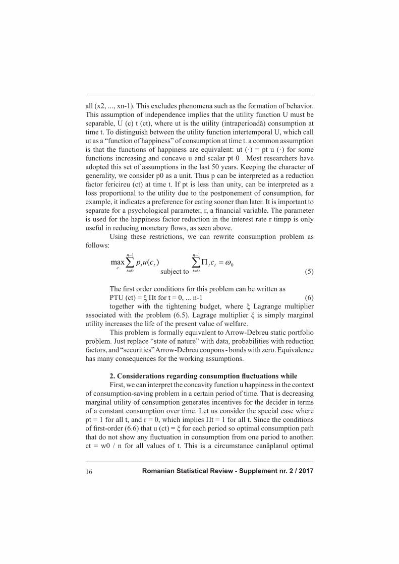
losses in consumption is suffi ciently small k is defi ned as

u̕(y0) = (1 + k)u̕ ( y1).

The left side of this equality is the marginal cost of reducing

consumption today, while the right side represents the marginal benefi t of

future growth in consumption by factor 1 + k. In other words, k can be defi ned

so that the loss of utility marginalăprin divest a unit of consumption at time 0

must equal marginal increase his usefulness by adding 1 + k consumer units

when Y1 is close to y0 1. If I use fi rst-order Taylor expansion of u (y0) to get

closer to y1

−−≅

)('

)(''

1

11

1

01

yu

yuy

y

yyk

(7)

Romanian Statistical Review - Supplement nr. 2 / 201718

Resistance to inter-temporal substitution is approximately proportional to the rate of increase in consumption. The multiplication factor, (y) = ̕-Yu (y) /

u (y) is also called the measure aversion fl uctuation relative or relative degree

of resistance to intertemporal substitution of consumption. Obviously, (y) is

similar measure relative to risk aversion Arrow -Pratt model. Both assesses

the percentage decreasing marginal utility with respect to a minor percentage

increase in wealth or consumption. Currently, we can consider a local measure

of consumer aversion to postpone consumption to once or time consuming to

one with low consumption slightly increased. In this regard, attention should

be given greater empirical estimates of (y), considered somewhere between 1

and 5.

3. Consumption with certainty - increase optimal

In principle, the real interest rate is zero, which feeds anxiety

agents makers. Suppose that consumers are calling the discount principle

exponentially, p1 = t for scalar less than 1. This implies a yield of pure

preference rate at the present time (1) / positive value. In other words, -1 and

happiness rate u (ct) multiplied by t is equivalent to happiness decrease at a

constant rate for that time period. Using a constant rate reductions subsequent

utilities is important for temporal consistency in consumer decisions, as will

be seen below.

Impatience and a positive profi t in saving has two balancing reasons so as not to equalize consumption over time. A high level of impatience, or higher, causing agents need to consume earlier that time. In other words, impatience tends to question the ways consumer preference in favor of that decrease over time. These two contradictory effects to be combined with aversion to fl uctuations in consumption, in order to achieve optimal growth

characterizations safe consumption.

Analytical problem solving exemplify this particular function if

happiness presents a constant degree of aversion to fl uctuations in consumption.

Using Arrow-Debreu model analogy, we get the solution

ct = c0 at (8)

where:

γ

δ

/1

1

1

++

=r

a

and c0 is a consumer initially chose to meet budget constraints across

lifetimes. Thus, when the reduction is exponential psychological and relative

Revista Română de Statistică - Supliment nr. 2 / 2017 19

aversion is constant, the consumer is best to keep consumption growth at a constant rate g, where

γδ

δ

γ−

≅−

++

≡rr

g 11

1/1

(9) Approximation is closer when not much different from r. Optimum consumption growth rate is positive when above. This property is maintained independently of happiness accurate function. This is where speculative facvoarea caremotivul saving effect dominates forward. Notice here and intuitive aversion effect of fl uctuations: an increase in the rate of growth

reduces consumption while optimal. But balance is optimal for complete

consumption throughout life only when r =, as happened when I was r =

.

Conclusion

In the real world, consumption growth is ascribed business cycles,

which put pressure on consumption fl uctuation over time. It has been debated

over the past 30 years. This cycle was found to have a negative impact on

well-being. Forcing her to collapse equalization cycles productive, we benefi t consumers whom dislike anyway fl uctuations in consumption growth rate

optimal g. In 1987, Lucas shows that important effect induced business cycle

on welfare has been overrated by specialists . It can measure the business

cycle cost by reducing consumption growth rate that the agent would accept

in exchange for complete elimination cycle afeceri. Using information

concerning fl uctuations of the US consumption, Lucas says that “price”

business cycle consists of a reduction than one-tenth less than one percent of

the annual growth rate of the US economy, which is totally insignifi cant. The reason is simple: the same as for the risk aversion we deal with the effect of second-order model additional EU aversion to fl uctuations in consumption as

a result of second order present in the model plus the temporal dimension of

model. In other words, consumers have an aversion to fl uctuations in extremely

low consumption low. Lucas concluded that economists should be concerned

rather the characteristics of long-term growth than reducing volatility.

Bibliografi e

1. Anghelache, C., Anghel, M.G. (2016). Econometrie generală. Concepte, teorie şi

studii de caz, Editura Artifex, Bucureşti

2. Anghelache, C., Anghelache, G.V., Sacală, C. (2016). Aspecte generale privind

evoluţia investiţiilor de capital în România / General Aspects on Developments in

Equity Investments in Romania, Romanian Statistical Review Supplement, Issue

4/2016, pg. 74-82/83-90

Romanian Statistical Review - Supplement nr. 2 / 201720

3. Anghelache, C., Manole, A., Anghel, M.G. (2015). Unifactorial Econometric Model - Connection between the Final Consumption and the Private Consumption, Asian Academic Research Journal Of Social Science & Humanities, Volume 2,

Issue 6, November 2015, pp. 212-219

4. Anghelache, C., Manole, A., Dumitrescu, D. (2015). The Correlation between Final Consumption, Gross Available Income and Gross Investment: An Econometric Analysis, International Journal of Academic Research in Accounting, Finance and

Management Sciences, Volume 5, No. 4, October 2015, pp. 84-88

5. Anghelache, C., Manole, A., Anghel, M.G. (2015). Analysis of fi nal consumption

and gross investment infl uence on GDP – multiple linear regression model,

Theoretical and Applied Economics, No. 3/2015 (604), Autumn, pg 137-142

6. Anghelache, C., Anghel, M.G. (2014). Modelare economică. Concepte, teorie şi

studii de caz, Editura Economică, Bucureşti

7. Anghelache, C. (2008). Tratat de statistică teoretică şi economică, Editura

Economică, Bucureşti

8. Cummins, J., Hassett, K., Oliner, S. (2006). Investment Behavior, Observable

Expectations, and Internal Funds, American Economic Review 96, no. 3, pp. 796-810

9. Deaton, A. (1991). Saving and liquidity constraints, Econometrica, 59

10. Dornbusch, R., Fischer, S., Startz, R. (2007). Macroeconomie - traducere, Editura

Economică, Bucureşti

11. Epstei, L.G., Zin, S.. (1991). Substitution, risk aversion and temporal behaviour

of consumption and assets returns: an empirical framework, Journal of political

economy, 99

12. Greenwood, R., Shleifer, A. (2014). Expectations of Returns and Expected

Returns, Review of Financial Studies 27, no. 3, pg. 714-746

13. Kimball, M.S. (1990). Precautionary cavings in the small and in the large,

Econometrica 58

14. Rampini, A.A., Viswanathan, S. (2010). Collateral, risk management, and the

distribution of debt capacity, Journal of Finance 65, 2293–2322

Revista Română de Statistică - Supliment nr. 2 / 2017 21

Precauţiunea economisirii în condiţii de incertitudine

Prof. univ. dr. Constantin ANGHELACHE

Academia de Studii Economice din București

Universitatea „ARTIFEX” din București

Conf. Univ. Dr. Aurelian DIACONU

Universitatea „ARTIFEX” din București

Drd. Emilia STANCIU

Academia de Studii Economice din București

Abstract

Problema certitudinii, a siguranței care infl uențează comportamentul decidentului, reprezintă un aspect cu dublă determinare: subiectivă și obiectivă. Într-o perspectivă temporală largă cu referire la orizontul integral al vieții decidentului, aspectele legate de factorii care constrâng sau relaxează comportamentul decizional se adună sub arcul de defi niție subiectivă al rezistenței și aversiunii față de fl uctuațiile consumului, dar și față de risc, devenit astfel parte din cadrul decizional subîntins întregii vieți a decidentului. Raportul dintre consum și siguranța decizională reprezintă un factor care asigură creșterea sau, după caz, descreșterea consumului. În momentul în care se instalează condiții de nesiguranță, decidentul va înclina comportamental către economisire, în ideea asigurării unei anumite fl uențe a consumului în timp, dar și a propriei existențe. Ideea unui comportament precaut nu ii este străină decidentului în asemenea circumstanțe, dar nici aceea a economisirii riscante, subiect necesar de defi nit și clarifi cat. Cuvinte cheie : venit, incertitudine, economisire, planifi care, consum Clasifi care JEL : E20, E21

Introducere

Presupunerea conform careia consumatorii au un venit constant este, in mod evident, o supozitie nerealista. Astfel, suntem nevoiti sa introducem nesiguranta in acest tablou general. Consumatorul ar putea planifi ca stiind ca

viitorul lui castig din munca este supus unor schimbari iar acesta ar putea fi

mai mare sau mai mic decat anticipase anterior.

Incertitudinea care afecteaza veniturile viitoare aduce un nou

motiv pentru a economisi. Banuiala este ca aceasta pune presiune asupra

consumatorilor sa creasca acumularea de bunastare tocmai pentru a se pregati

sa infrunte un risc viitor. Acesta este asa-numitul motiv de precautie pentru

economisire si el consta intr-un comportament prudent de consum.

Romanian Statistical Review - Supplement nr. 2 / 201722

1. Noţiuni generale introductive

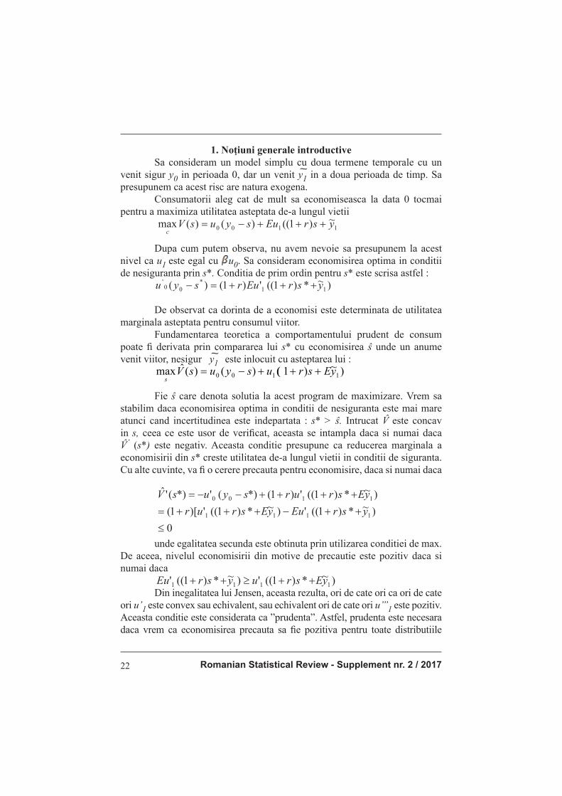
Sa consideram un model simplu cu doua termene temporale cu un venit sigur y0 in perioada 0, dar un venit y͠1 in a doua perioada de timp. Sa presupunem ca acest risc are natura exogena. Consumatorii aleg cat de mult sa economiseasca la data 0 tocmai pentru a maximiza utilitatea asteptata de-a lungul vietii

asteptata de-a lungul vietii

1100~)1(()()(max ysrEusyusV

c

Dupa cum putem observa, nu avem nevoie sa presupunem la acest nivel ca

~

Dupa cum putem observa, nu avem nevoie sa presupunem la acest nivel ca u1 este egal cu u0. Sa consideram economisirea optima in conditii de nesiguranta prin s*. Conditia de prim ordin pentru s* este scrisa astfel :

)~*)1((')1()( 11

*

00' ysrEursyu

De observat ca dorinta de a economisi este determinata de utilitatea marginala asteptata pentru consumul viitor. Fundamentarea teoretica a comportamentului prudent de consum poate fi derivata prin compararea lui s* cu economisirea ŝ unde un anume

venit viitor, nesigur y͠1 este inlocuit cu asteptarea lui :

)~)1(()()(ˆmax 1100 yEsrusyusV

s+++−=

Fie ŝ care denota solutia la acest program de maximizare. Vrem sa

stabilim daca economisirea optima in conditii de nesiguranta este mai mare

atunci cand incertitudinea este indepartata : s* > ŝ . Intrucat V̂ este concav

in s, ceea ce este usor de verifi cat, aceasta se intampla daca si numai daca

V̂’ (s*) este negativ. Aceasta conditie presupune ca reducerea marginala a

economisirii din s* creste utilitatea de-a lungul vietii in conditii de siguranta.

Cu alte cuvinte, va fi o cerere precauta pentru economisire, daca si numai daca

precauta pentru economisire, daca si numai daca

0

)~*)1((')~*)1((')[1(

)~*)1((')1(*)('*)('ˆ

1111

1100

ysrEuyEsrur

yEsrursyusV

unde egalitatea secunda este obtinuta prin utilizarea conditiei de max. De aceea, nivelul

~

unde egalitatea secunda este obtinuta prin utilizarea conditiei de max.

De aceea, nivelul economisirii din motive de precautie este pozitiv daca si

numai daca

)~*)1((')~*)1((' 1111 yEsruysrEu

Din inegalitatea lui Jensen, aceasta rezulta, ori de cate ori ca ori de cate ori Din inegalitatea lui Jensen, aceasta rezulta, ori de cate ori ca ori de cate

ori u’1 este convex sau echivalent, sau echivalent ori de cate ori u’’’1 este pozitiv.

Aceasta conditie este considerata ca ”prudenta”. Astfel, prudenta este necesara

daca vrem ca economisirea precauta sa fi e pozitiva pentru toate distributiile

Revista Română de Statistică - Supliment nr. 2 / 2017 23

posibile ale riscului viitor. Un consumator cu o functie de utilitate marginala concava, dimpotriva, va reduce economisirile din cauza riscului viitor. Acest individ va manifesta ceea ce se numeste ”comportament imprudent”. Astfel, prudenta corespunde pozitivitatii celei de a treia derivate a functiei de utilitate la fel cum aversiunea fata de risc se bazeaza pe negativitatea derivatei secunde. Un agent poate exprima un comportament advers fata de risc si imprudent, de exemplu, asigurandu-si riscul printr-o prima de risc incorecta si reducandu-si economiile fata in fata cu un risc viitor neasigurat. Astfel, conform defi nitilor,

o persoana prudenta ar putea fi considerata iubitoare de risc. Exista o legatura

totusi intre aversiunea de risc descrescatoare si prudenta. Intrucat consideram

aversiunea descrescatoare fata de riscul absolut (DARA) ca pe o supozitie

naturala, la fel ar trebui sa consideram si prudenta.

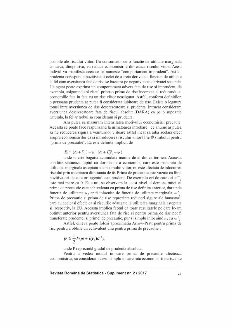
Am putea sa masuram intensitatea motivului economisirii precaute.

Aceasta se poate face raspunzand la urmatoarea intrebare : ce anume ar putea

sa fi e reducerea sigura a veniturilor viitoare astfel incat sa aiba acelasi efect

asupra economisirilor ca si introducerea riscului viitor? Fie simbolul pentru

”prima de precautie”. Ea este defi nita implicit de

simbolul pentru ”prima de precautie”. Ea este definita implicit de

)(')(' 1111 yEuyEu

este bogatia acumulata inainte de al doilea termen. Aceasta conditie statueaza faptul ca unde w este bogatia acumulata inainte de al doilea termen. Aceasta

conditie statueaza faptul ca dorinta de a economisi, care este masurata de

utilitatea marginala asteptata a consumului viitor, nu este afectata de inlocuirea

riscului prin asteptarea diminuata de . Prima de precautie este vazuta ca fi ind

pozitiva ori de cate ori agentul este prudent. De exemplu ori de cate ori u’’’1 este mai mare ca 0. Este util sa observam la acest nivel al demonstratiei ca

prima de precautie este echivalenta cu prima de risc defi nita anterior, dar unde

functia de utilitatea u1 ar fi inlocuita de functia de utilitate marginala -u’1.

Prima de precautie si prima de risc reprezinta reduceri sigure ale bunastarii

care au aceleasi efecte ca si riscurile adaugate la utilitatea marginala asteptata

si, respectiv, la EU. Aceasta implica faptul ca toate rezultatele pe care le-am

obtinut anterior pentru aversiunea fata de risc si pentru prima de risc pot fi

transferate prudentei si primei de precautie, pur si simplu inlocuind u1 cu -u’1.

Astfel, cineva poate folosi aproximatia Arrow-Pratt pentru prima de

risc pentru a obtine un echivalent unu pentru prima de precautie :

1

~2

1 )(2

1yyEP σωψ +≅

unde P reprezintă gradul de prudenta absoluta. Pentru a vedea modul in care prima de precautie afecteaza economisirea, sa consideram cazul simplu in care rata economisirii neriscante

Romanian Statistical Review - Supplement nr. 2 / 201724

egaleaza rata reducerii pentru preferinta temporala, si le stabilim pe amandoua ca fi ind egale cu 0, de exemplu r= =0. In particular, utilitatea pe viata este

considerata a fi U(c0,c1) = u(c0) + u(c1). Presupunem, de asemenea, Ey͠

1=y0, astfel ca individul are acelasi venit asteptat atat la momentul 0 cat si la

momentul 1. Sa presupunem, mai intai, ca ỹ 1 este neriscant, adica ỹ 1 ỹ 0.

In aceasta formula, conditia de prim ordin (6.11) implica faptul ca u’(y0-s)

= u’(y0+s). Asa cum observam deja rezulta ca economisirea optima este 0,

s*=0, de vreme ce u este strict concava. Cu alte cuvinte, consumatorul pur si

simplu isi consuma venitul curent in fi ecare perioada : c*0 = c*1 = y0.

Acum sa presupunem ca y͠ 1 este riscant, astfel ca conditia de ordin

prim este

)(')~(')(' 010 syusyEEusyu

A doua egalitate de mai sus deriva din defi nita noastra asupra primei

de precautie. Rezolvarea pentru economisirea optima da s*= ½ Astfel,

atunci cand consumatorul este prudent el va manifesta o cerere precauta

de economisiri, s*>0. Mai mult, un individ care este mult mai prudent va

avea o valoare mai mare a primei de precautie , in acelasi mod in care un

individ care o aversiune mai mare fata de risc are o prima de risc mai mare.

Rezulta ca un consumator mai prudent va economisi mai mult decat unul mai

putin prudent. Este foarte interesant de vazut ca daca functia de fericire este

cuadratica ceea ce reprezinta o presupunere mai putin comuna literaturii din

acest domeniu, vom avea = 0, ceea ce inseamna inexistenta unui motiv

de economisire precauta.

Literature review

Anghelache şi Anghel (2016), Anghelache et.al. (2006) descriu

instrumentele statistice utilizate în măsurarea indicatorilor macroeconomici.

Anghelache, Manole şi Anghel (2016) abordează caracteristica de normalitate

asimptotică a estimatorilor de ecuaţie singulară. Anghelache (2016),

Dougherty (2007) se preocupă de conceptele teoretice legate de instrumentele

econometrice, Anghelache, Manole şi Anghel (2015) studiază instrumentele

modelării economice, fi nanciar-bancare şi informatice. Anghelache şi Sacală

(2014) descriu caracteristicile mediului de afaceri românesc prin prisma

investiţiilor de capital. Bloom (2009) evaluează impactul incertitudinii,

Bloom, Bond şi Van Reenen (2007) analizează impactul incertitudinii asupra

investiţiilor, Bolton, Wang şi Yang (2014), Grenadier şi Wang (2007) dezvoltă

pe teme apropiate. Hafner şi Wallmeier (2008) se concentrează pe volatilitate

ca factor de infl uenţă asupra investiţiilor. Itzhak, Graham şi Campbell (2013)

studiază o serie de riscuri de ordin psihologic şi economic care se manifestă

la nivelul managementului. Miles (2009) analizează efectele incertitudinii

Revista Română de Statistică - Supliment nr. 2 / 2017 25

asupra investiţiilor. Salman şi McLee (2014) au în vedere relaţia dintre

investiţia agregată şi sentimentele investitorilor.

2. Corelaţia dintre economisirea riscantă si cererea precaută

Anterior am considerat numai riscul legat de venitul din munca.

Individul avea o alternativa de economisire fara risc dar era nesigur in legatura

cu marimea venitului pe care il va castiga la momentul 1. Avand in vedere un

model in care venitul din munca este cunoscut, dar rata profi tului din economii

este riscanta. Sa consideram un consumator cu un orizont investitional de

doua perioade. In cazul in care venitul de-a lungul vietii este cunoscut cu

certitudine, presupunem fara a pierde caracterul de generalitate ca intregul

venit este platit la data t=0. Presupunem ca w0 denota aceasta bunastare.

Obiectivul consumatorului este

))~1(()()(max 0 srEususV

s

~~

~~

Conditia de ordin prim pentru acest program este

))1((')1()(' 000 srursu

~~

Conditia de ordin secund este mai usor de indicat ca derulandu-se sub

aversiunea fata de risc. In fapt, functia obiectiva V(s) este concava in s.

Sa consideram, in primul rand, cazul in care rata economisirii lipsita

de risc este r0 ca anterior. Conditia de ordin prim in acest caz devine

))1((')1()(' 000 srursu ++=− βω

Concentrandu-ne asupra efectelor riscului consideram inca o data

cazul simplu in care rata de profi t asteptata a economiilor egaleaza rata de

discount pentru preferinta de timp, de exemplu, r= , astfel ca =(1+r0)-1.

Totusi, s* satisface

w0-s*=(1+r0)s*. Asa cum era de asteptat economia optimala s* este astfel

considerata incat nu exista nici o fl uctuatie in consum intre cele doua date :

c*0=c*1. Revenim la chestiunea daca adaugand risc la profi tul din economisiri

se obtine un nivel mai mare de economisire, in aceasta formula rezulta ca

prudenta singura nu este sufi cienta pentru a conduce la o crestere de nivel a

economisirii. In fapt, exista doua infl uente care contribuie la aceasta, pe de

o parte caracterul riscant al profi tului face economisirile mai putin atractive

decat o rata libera de risc cu acelasi profi t mediu. Dar, pe de alta parte, termenul

1 al riscului va induce un motiv de precautie consumatorului prudent. Rezulta

ca avem nevoie de un nivel de prudenta sufi cient de ridicat pentru a avea o

dominatie a motivului de precautie asa cum vom arata in continuare.

De vreme ce V(s) este concav, rezulta ca nesiguranta in rata profi tului

va forta nivelul optim al economisirilor ori de cate ori este satisfacuta relatia :

))1((')1()])~1((')~1[( 00 srursrurE

Aceasta inegalitate se sustine daca functia h(R) Ru’(Rs) este convex in R. Calculul corect arata

Romanian Statistical Review - Supplement nr. 2 / 201726

Aceasta inegalitate se sustine daca functia h(R) Ru’(Rs) este convex in R. Calculul corect arata ca h’’(R)=2su’’(Rs)+s2Ru’’’(Rs). Sa presupunem ca u’’<0 si ca economisirile nu sunt 0, de vreme ce c1 ar fi tot zero, in acest caz.

Rezulta ca h’’>0 daca

ar fi tot zero, in acest caz. Rezulta ca h’’>0 daca

2)(''

)('''

zu

zzu

Partea stanga a ecuatiei este doar o se sustine cu z=Rs. Partea stanga a ecuatiei este doar o masura

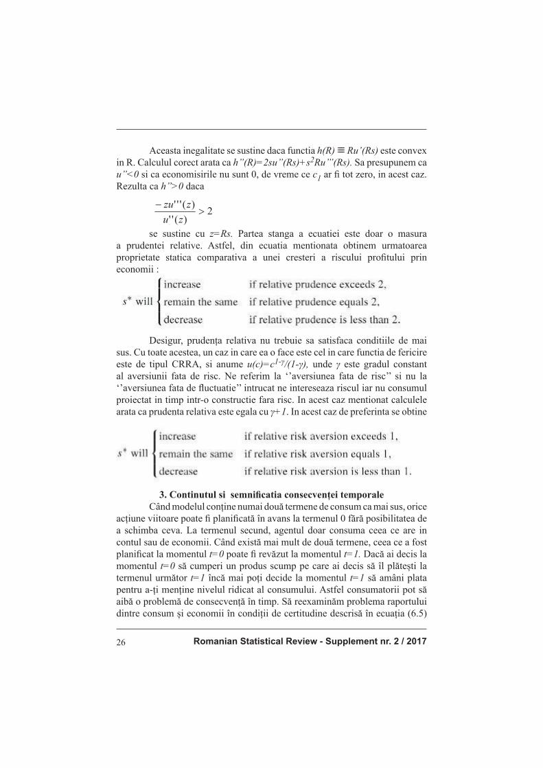
a prudentei relative. Astfel, din ecuatia mentionata obtinem urmatoarea

proprietate statica comparativa a unei cresteri a riscului profi tului prin

economii :

Desigur, prudența relativa nu trebuie sa satisfaca conditiile de mai sus. Cu toate acestea, un caz in care ea o face este cel in care functia de fericire este de tipul CRRA, si anume u(c)=c1-γ/(1-γ), unde γ este gradul constant al aversiunii fata de risc. Ne referim la ‘’aversiunea fata de risc’’ si nu la ‘’aversiunea fata de fl uctuatie’’ intrucat ne intereseaza riscul iar nu consumul proiectat in timp intr-o constructie fara risc. In acest caz mentionat calculele arata ca prudenta relativa este egala cu γ+1. In acest caz de preferinta se obtine

3. Continutul si semnifi catia consecvenței temporale

Când modelul conține numai două termene de consum ca mai sus, orice acțiune viitoare poate fi planifi cată în avans la termenul 0 fără posibilitatea de a schimba ceva. La termenul secund, agentul doar consuma ceea ce are in contul sau de economii. Când există mai mult de două termene, ceea ce a fost planifi cat la momentul t=0 poate fi revăzut la momentul t=1. Dacă ai decis la momentul t=0 să cumperi un produs scump pe care ai decis să îl plătești la termenul următor t=1 încă mai poți decide la momentul t=1 să amâni plata pentru a-ți menține nivelul ridicat al consumului. Astfel consumatorii pot să aibă o problemă de consecvență în timp. Să reexaminăm problema raportului dintre consum și economii în condiții de certitudine descrisă în ecuația (6.5)

Revista Română de Statistică - Supliment nr. 2 / 2017 27

unde Пt=(1+r)-t si n 3. La momentul t=0 consumatorul iși planifi că profi lul de consum (c0 ,…, cn-1) pentru restul vieții lui, ceea ce maximizează utilitatea

duratei vieții 0

1

)( ω=∑−

=

n

ot

tt cup care este supusă restricțiilor de buget de-a

lungul vieții 0

1

ω=Π∑−

=

n

ot

tt c . Să ne amintim că pt este factorul folosit pentru a

determina scăderea fericirii la momentele t din ciclul curent. Folosind condiția pentru t=1și t=0, alegerea planifi cată este de forma:

)(')1(

)(' 12

12 cu

pr

pcu

+= .

Această regulă de consum poate fi satisfăcută astfel încât să se cheltuie efi cient banii economisiți la momentul t=0. Anticipând modul în care va cheltui banii economisiți, agentul își determină consumul optim inițial c0. Rezolvând sistemul de ecuații rezultat împreună cu restrângerea de buget, întregul profi l al consumului este selectat astfel: (c0, c1, c2, ... , cn-1) Să considerăm situația generată la momentul t=1. Bunăstarea a fost efectivă prin consumul inițial c0, dar a și crescut pe baza profi tului r din economisire. La momentul t=0, agentul a planifi cat să consume c1 la momentul t=1. Cu toate acestea, el este gata să își reconsidere alegerea. Bunăstarea pentru perioada rămasă poate fi scrisă:

∑−

=−

1

1 )(n

ot

tt cup .

Indexurile parametrilor p și variabilelor c sunt importante în acest moment. În particular trebuie remarcat, că satisfacţia u(c2) care are loc la o perioadă distanță t=1 este micșorată în punctul p1, factorul de micșorare pentru orizontul unei perioade. Maximizând funcția obiectivă cu restrângerea bugetului obţinem:

)1)(( 00

1

1 rcc

n

ot

tt, ceea ce genereaz, ceea ce generează condiția de ordin

prin alegerea actuală: )(')1(

)(' 11

02 cu

pr

pcu

+=

Ecuațiile de mai sus sunt echivalente numai dacă p1/p2=p0/p1. Aceasta echivalează cu o cerere pt=aβt pentru t=0,1,2, sau acea scădere să fi e

Romanian Statistical Review - Supplement nr. 2 / 201728

exponențială. Această terminologie decurge din faptul că echivalentul timp-continuu al acestei funcții de scădere este p(t) = e-δt. Extinderea acestei condiții pentru toate momentele t implică faptul că alegerea de consum optimă c1 se localizează în momentul t=1 și nu este diferită de cea care a fost planifi cată la momentul t=0.

Concluzii

Problema este mult mai complexă atunci când consumatorul nu

folosește condiţia pt=aβt pentru factorii de scădere. Presupunem că p2 este mai

cuprinzător decât relaţia p /p0. Din ecuațiile iniţiale rezultă că nivelul de consum

c1 selectat la momentul t=1 este mai mare decât cel planifi cat la momentul t=0. În acest caz avem o problemă de consistență. Când determină consumul inițial, agentul nu poate avea încredere în el insuși în legătură cu limitarea propriului consum în viitor. Aceasta este tipic pentru comportamentul adictiv: un consumator consideră că este bine pentru el să consume astăzi în funcție de convingerea sa că va renunţa la consum mâine dar când vine ziua de mâine consumatorul descoperă că este bine pentru el să consume, amânând astfel pe mâine decizia de a nu mai consuma în ziua următoare, și așa mai departe. Putem suspecta că un asemenea comportament adictiv se poate extinde și asupra altor produse generând o problemă globală de adicție în consum. Pentru oamenii care au această problemă, planurile de economisire pe termen lung fără posibilitatea de a retrage bani pot să fi e benefi ce în pofi da infl exibilității acestor planuri. Problema consistenței temporale poate explica de ce un număr mare al populației din țările dezvoltate găsește acceptabil să fi nanțeze consumul pe termen scurt cu împrumuturi prin cărți de credit la rate de 20% și încă să păstreze bani în conturi de economie pe termen lung cu rate sub 5%.

Bibliografi e

1. Anghelache, C., Anghel, M.G. (2016). Bazele statisticii economice. Concepte

teoretice şi studii de caz, Editura Economică, Bucureşti 2. Anghelache, C., Manole, A., Anghel, M.G. (2016). Asymptotic Normality for

Single Equation Estimators for Population with Sensitive Instrument, Economica, Scientifi c and didactic journal, Year XXIV, nr. 2 (96), June 2016, pp. 124-130

3. Anghelache, C. (2016). Econometrie teoretică – Ediţia a II-a revizuită, Editura Artifex, Bucureşti

4. Anghelache, C., Manole, A., Anghel, M.G. (2015). Modelare economică, fi nanciar-

bancară şi informatică, Editura Artifex, Bucureşti 5. Anghelache, C., Sacală, C. (2014). The Autochtonous Investments and the Business

Environment, Romanian Statistical Review Supplement no. 10/2014 6. Anghelache, C., Isaic-Maniu, A., Mitruţ, C., Voineagu, V., Dumbravă, M., Manole,

A. (2006). Analiză macroeconomică: teorie şi studii de caz, Editura Economică, Bucureşti

Revista Română de Statistică - Supliment nr. 2 / 2017 29

7. Bloom, N. (2009). The Impact of Uncertainty Shocks, Econometrica 77, no. 3, pg. 623-685

8. Bloom, N., Bond, S., Van Reenen. J. (2007). Uncertainty and Investment Dynamics, Review of Economic Studies 74, no. 2, pp. 391-415

9. Bolton, P., Wang, N., Yang, J. (2014). Investment under uncertainty and the value

of real and fi nancial fl exibility, National Bureau Of Economic Research Working Paper Series issued in October 2014, Cambridge

10. Dougherty, C. (2007). Introduction to Econometrics, Oxford University Press 11. Grenadier, S.R., Wang, N. (2007). Investment under uncertainty and time-

inconsistent preferences, Journal of Financial Economics 84, pp. 2-39 12. Hafner, R., Wallmeier, M. (2008). Optimal investments in volatility, Financial

Markets and Portfolio Management, v. 22, iss. 2, pp. 147-67 13. Itzhak, B.D., Graham, J., Campbell, H.(2013). Managerial Miscalibration,

Quarterly Journal of Economics 128, no. 4, pp. 1547-1584 14. Miles, W. (2009). Irreversibility, Uncertainty and Housing Investment, Journal of

Real Estate Finan Econ, 38, pg. 173–182 15. Salman, A., McLee, Ch. (2014). Aggregate Investment and Investor Sentiment,

Review of Financial Studies 27, no. 11, pg. 3241-3279

Romanian Statistical Review - Supplement nr. 2 / 201730

PRECAUTION OF SAVINGS UNDER UNCERTAIN CIRCUMSTANCES

Prof. Constantin ANGHELACHE PhD.

Bucharest University of Economic Studies, „ARTIFEX” University of Bucharest

Assoc. prof. Aurelian DIACONU PhD.

„ARTIFEX” University of Bucharest

Emilia STANCIU PhD. Student

Bucharest University of Economic Studies

Abstract

The problem of certainty, of safety which infl uences the decision-makers’

behaviour is both subjective and objective. In a wide temporal perspective with

reference to the full horizon of the decision-maker’s life, the aspects related to the

factors that constrain or relax the decisional behavior gather under the umbrella of the

subjective defi nition of resistance and aversion to fl uctuations in consumption, but also

to risk, thus becaming part of the decision framework in the decision maker’s lifetime.

The ratio between consumption and safe decision-making is a factor

that ensures the increase or the decrease in consumption. Under unsafe

conditions, the decision-maker will incline towards a saving behaviour, with the

view to ensuring a certain continuity in consumption, but also with the benefi t of

ensuring his own existence. Neither the idea of a cautious behavior, nor that of

risky saving is foreign to the decision-maker in such circumstances, that being

an issue necessary to defi ne and clarify.

Keywords: income, uncertainty, savings, planning, consumption

JEL Classifi cation: E20, E21

Introduction

The assumption that consumers have a steady income is obviously unrealistic. Thus, we have to introduce uncertainty in this overview. The consumer should be able to plan knowing that his future earnings from work is subject to changes and they could be higher or lower than expected. Uncertainty affecting future income brings a new reason to saving. The supposition is that this puts pressure on consumers to increase the accumulation of wealth in order to prepare to face a future risk. This is the so-called precautionary reason for saving and it consists of a cautious consumer behavior.

1. Introductory general notions

Let us consider a simple model with two time periods with a secure income y0 during a period 0, but an income y͠1 in the second period. Suppose that risk is exogenous.

Revista Română de Statistică - Supliment nr. 2 / 2017 31

Consumers choose how much to save at the time 0 in order to maximize the utility of they expected all along:

���������������� ���������!

������

�

�

�

��

��

As we can notice, we do not need to suppose at this level is that u1 equal to u0. Let us consider s* as optimal saving under uncertain conditions. The fi rst order condition for s* is written as follows:

������������ ��

���

��������� �����

�

�

�

��

Note that the desire to save is determined by the marginal utility of

consumption expected in the future.

Theoretical cautious consumer behaviour can be derived by comparing

s* with savings ŝ , where ŝ a certain insecure future income y͠1 is replaced by

its expectation:

�������������� ���� ���������!

������

�

��

��

Let us consider ŝ as the solution to this maximization program.

We want to establish whether optimal savings under uncertain conditions is

bigger when uncertainty is removed: s* > ŝ . Since V̂ is concave in s, which is

easily verifi able, this happens if and only if V̂’ (s*) is negative. This condition

implies that by marginal decrease in saving of s* , we increase the utility in

the long run, under certain conditions. In other words, there will be a demand

for cautious savings, if and only if:

�

������������������

�����������������

����

����

�

�������

�������

�����������

����������!

��

where the second equality is achieved by using the max condition.

Therefore, the level of savings out of cautious reasons is positive if and only

if:

�������������� ���� ���������� ������

From Jensen’s inequality, this results whenever u’1 is convex or

equivalent, or when u’’’1 is positive. This condition is considered „cautious”.

Thus, caution is needed if we want prudent saving to be positive for all

possible distributions of the future risk. A consumer with a concave function

of marginal utility, on the contrary, will reduce future savings because of the

future risk. This individual will manifest what is called „reckless behavior”.

Thus, caution corresponds to the third derivative’s positivity of the utility

Romanian Statistical Review - Supplement nr. 2 / 201732

function just as risk aversion is based on the second derivative’s negativity. An agent may express an adversary and imprudent behaviour towards risk, for example, by ensuring the risk using an incorrect risk premium and reducing his savings in the case of a future uninsured risk. So, according to defi nition,

a prudent person could be considered a risk-loving person. Yet, there is a link

between decreasing risk aversion and caution. As we consider the decreasing

risk aversion toward absolute risk (DARA) as a natural assumption, we should

consider caution in the same way.

We could measure the intensity of the reason for cautious saving. This

can be done by answering the question: what can we consider a safe reduction

of future income so as to have the same effect on savings as placing future

risk? Where is the symbol of „bonus caution”. It is implicitly defi ned by:

�

������ ���� ��� ���� ��������

�

�

,

where w is the wealth accumulated before the second term. This

condition means that the desire to save, which is measured by the expected

marginal utility of future consumption is not affected by replacing risk with the

diminishing expectation of . The caution bonus is seen as positive whenever

the agent is prudent. For example, whenever u’’’1 is bigger than 0. It is useful

to note at this level of demonstration, that caution bonus is equivalent to the

above mentioned risk bonus, but where utility function u1 would be replaced

by the function of marginal utility -u’1. The caution bonus and the risk bonus

represent cuts in the welfare, and they have the same effects as the risks added

to the expected marginal utility, respectively to EU. This implies that all the

results that we previously obtained for risk aversion and risk bonus can be

transferred to prudence and caution bonus, by simply substituting u1 with u’1.

Thus, one can use Arrow-Pratt approximation for the risk bonus in order to

obtain an equivalent one for the fi rst caution bonus:

1

~2

1)(2

1yyEP σωψ +≅

where P represents the degree of absolute caution.

In order to observe to what extent the caution bonus affects savings,

let us consider the simple case in which the rate of non-risky savings equals

the rate of reduction for time preference, and establish both of them as being

equal to 0, ie r=

�!���,�������������������� ��������������

�,�,�

�

=0. In particular, a life-time utility is considered to be

U(c0,c1) = u(c0) + u(c1). We also suppose that Ey͠ 1=y0 so that the individual

has the same income expected at time 0 and at time 1. Let us suppose, at fi rst,

that ỹ 1 is non-risky, that meaning that ỹ 1 ỹ 0. In this formula, the fi rst order

condition (6.11) implies that u’(y0-s) = u’(y0+s). As already notice, optimal

Revista Română de Statistică - Supliment nr. 2 / 2017 33

savings is 0, s*=0, since u is strictly concave. In other words, the consumer simply uses his regular income in each period: c*0 = c*1 = y0. Now let us suppose that y͠ 1 is risky, so the fi rst order condition is:

���������� ��� ������� ������������

The second equality above derives from our defi nition of the caution

bonus. By solving optimal savings, we obtain s*= ½�������������������!!��� ������������������������������������� �����������������������

��!�����������������������������������!!��������

�� ��

�� ��

. Thus, when the consumer

is cautious, he will manifest a cautious request for savings, s*>0. Furthermore,

an individual who is more prudent will have a bigger caution bonus �������������������!!��� ������������������������������������� �����������������������

��!�����������������������������������!!��������

�� ��

�� ��

, in the

same way in which an individual who has a greater aversion to risk will have a

bigger risk bonus. We conclude that a more cautious consumer will save more

than one less prudent. It is very interesting to see that if the happiness function is

a quadratic function, which represents a less common assumption in this fi eld,

so we have �������������������!!��� ������������������������������������� �����������������������

��!�����������������������������������!!��������

�� ��

�� ��

= 0, which means the inexistence of a reason for cautious savings.

Literature review

Anghelache and Anghel (2016), Anghelache (2006) describe the

statistical tools used to measure the macroeconomic indicators. Anghelache,

Manole and Anghel (2016) use the asymptotic normality feature of estimators

of singular equation. Anghelache (2016), Dougherty (2007) are concerned with

theoretical concepts related to econometric tools, Anghelache, Manole and

Anghel (2015) study the tools of economic, fi nancial and banking information

models. Anghelache and Sacala(2014) describe the characteristics of the

Romanian business environment in terms of capital investment. Bloom (2009)

assess the impact of uncertainty, Bloom, Bond and Van Reenen (2007) analyze

the impact of uncertainty on investmentS, Bolton, Wang and Yang (2014),

Grenadier and Wang (2007) have similar preferences. Hafner and Wallmeier

(2008) focuse on volatility as an infl uencing factor on investment. Itzhak,

Graham and Campbell (2013) study a series of psychological and economic

risks that manifest at the level of management. Miles (2009) analyzes the

effects of uncertainty on investments. Salman McLee (2014) are concerned

with the relationship between aggregate investment and investors’ feelings.

2. The correlation between risky savings and cautious demand

In the analysis above we took into consideration only the work-related

risk. The individual had a chance of risk-free alternative savings but he was

not sure about the size of the income that he will earn at the given time 1.

considering a model in which labor income is known, but the profi t rate of

savings is risky. Let us consider a consumer with an investment horizon of

two periods. If a lifelong income is certain, we assume without losing the

Romanian Statistical Review - Supplement nr. 2 / 201734

generality that the entire income is paid at time t=0. Let us suppose that w0 signifi es wealth. The consumer’s target is:

������������� � �������!

���� ��

�� ���� ��

���� ��

The fi rst order condition for this program is:

��������������� � ������� ���� ��

���� ��

The second-order condition is easier to identify as unfolding under

the risk aversion. In fact, the objective function V(s) is concave in s.

Let us consider, fi rstly, the case in which the savings rate without risk

is r0 as before. The fi rst order condition in this case is:

������������ ��� ������ ���� ��

Focusing on the effects of risk once again we consider the simple

case in which the expected profi t rate savings equals discount rate for time

preference, ie r= �,���������� so that =(1+r0)-1. However, s* satisfi es w0-s*=(1+r0)s*.

As expected, optimal economy s* is thus considered as there is no fl uctuation

in consumption between the two data: c*0=c*1. We return to the question

whether adding risk to profi t from savings we obtain a higher level of savings,

in this formula we conclude that prudence alone is not suffi cient to lead to an

increase in the level of savings. In fact, there are two infl uences that contribute

to it, on the one hand, the risky nature of profi t makes savings less attractive

than a risk free rate with the same average profi t. But, on the other hand, the

term 1 of risk will induce a reason for caution to a prudent consumer. We

conclude that we need a prudency level high enough to have a dominance of

the reason for caution as we’ll demonstrate further in this article.

Since V(s) is concave, we conclude that the uncertainty of the profi t rate

will force optimum level of savings whenever the folllowing relation is satisfi ed:

���������������������� �� ��������� �����

�

�

This inequality is sustenable if the function h(R) Ru’(Rs) is convex

in R. A correct calculation shows that h’’(R)=2su’’(Rs)+s2Ru’’’(Rs). Let us

suppose that u’’<0 and that savings are not 0, since c1 would still be zero in

this case. We conclude that h’’>0 if:

�����

������

�

5�

55�

is sustained by z=Rs. The left side of the equation is just a measure of

the relative prudence. Thus, from the equation, we get the following property

of comparative statics of risk profi ts by saving:

Revista Română de Statistică - Supliment nr. 2 / 2017 35

Of course, the relative prudence should not satisfy the above mentioned conditions. However, a case in which it does, is the function of happiness of CRRA type, namely u(c)=c1-γ/(1-γ), where γ is the constant degree of risk

aversion . We refer to “risk aversion” and not to ”aversion fl uctuation” because

we are interested in risk and not in the consume projected in time in a risk-free

construction. In this case, calculations show that relative caution is equal to

γ+1. In this case, preference is obtained as follows:

3. The content and signifi cance of temporal consistency

When the model contains only two terms of consumption as above,

any future action can be planned in advance at 0 term with no possibility of

changing anything. At the second term, the agent only consumes what has in

his savings account. When there are more than two terms, which was planned

at time t=0 can be reviewed at time t=1. If you decided at t=0 to buy an

expensive product that you decided to pay him the next term t=1, you still can

decide at time t=1 to delay payment to keep your high level of consumption.

Thus, consumers can have a problem of consistency over time. Let us

reconsider the relation between consumption and savings under conditions

of certainty described in equation (6.5), where Пt=(1+r)-t and n3. At the time

t=0, the consumers plans his consumption profi le (c0 ,…, cn-1) for the rest

of his life, which maximizes the utility of life expectancy 0

1

)( ω=∑−

=

n

ot

tt cup

that is subject to budget restrictions throughout life 0

1

ω=Π∑−

=

n

ot

tt c . Let us

remember that pt is the factor used to decrease the happiness at times t in the

current cycle. Using the condition for t=1and t=0, the choice is planned as

follows:

)(')1(

)(' 1

2

12 cu

pr

pcu

+=

Romanian Statistical Review - Supplement nr. 2 / 201736

This rule of consumption can be satisfi ed so as to effectively spend

the money saved at time t=0. Anticipating how he will spend the money he

saved, the agent determines his initial optimal consumption c0. By solving the

system of equations resulted in the combination with reducing the budget, the

whole profi le of consumption is selected as follows:

(c0, c1, c2, ... , cn-1)

Let us consider the situation generated at time t=1. The welfare was

effective by the initial consumtion c0, but it has also increased based on the

profi t r resulted from savings. At time t=0, the agent planned to consume c1 at

time t=1. However, he is ready to reconsider his choice. The welfare for the

period which remained can be written as follows:

∑−

=−

1

1 )(n

ot

tt cup

Indexes of p parameters and c variables that are important at this moment.

In particular, we should notice that the satisfaction u(c2) which occurs at a time

t=1 is diminished in the point p1, the diminishing factor for the horizon of a period.

By maximizing the objective function and reducing the budget, we obtain:

����� ��

�

� ����

�

���� �

�

� �

which generates the prime order condition provided by the current

choice:

)(')1(

)(' 1

1

0

2 cupr

pcu

+=

The above equations are equivalent only if p1/p2=p0/p1. This is the

equivalent to a request for pt=aβt for t=0,1,2, or that fall to be exponential. This

terminology comes from the fact that the equivalent of the continuous time of

this decreasing function is p(t) = e-δt. Extending this condition for all times t implies that the fact that the choice of optimal consumption c1 is located in t=1

and is not different from the the one which was planned at time t=0.

Conclusion

The problem is more complex when the consumer does not use the

condition pt=aβt for the decreasing factors. Let us suppose that p2 is larger than

the relationship p/p0.. From the initial equations there comes the conclusion that

the consumption level selected c1 at time t=1is higher than the one planned at the

time t=0. In this case, we have a problem of consistency. When determining the

initial consumption, the agent can not trust himself in relation to limiting his own

Revista Română de Statistică - Supliment nr. 2 / 2017 37

consumption in the future. This is typical of an addictive behavior: a consumer believes that it is better for him to consume today based on his belief that it would give up the consumption tomorrow, but when tomorrow comes, the consumer realises that it is better for him to purchase, thus postponing the tomorrow’s decision to the next day, and so on. We may also suspect that such an addictive behavior can be extended to other products generating a global problem of addiction to consumption. For people who have this problem, long-term savings plans without the possibility of withdrawing money may be benefi cial despite

the infl exibility of these plans. The problem of temporal consistency may explain

why a large number of people in developed countries fi nd it acceptable to fi nance

consumption based on short-term loans by using credit cards at 20% interest, and

still keep money in long-term accounts with interests under 5 %.

Bibliography

1. Anghelache, C., Anghel, M.G. (2016). Bazele statisticii economice. Concepte

teoretice şi studii de caz, Editura Economică, Bucureşti

2. Anghelache, C., Manole, A., Anghel, M.G. (2016). Asymptotic Normality for

Single Equation Estimators for Population with Sensitive Instrument, Economica,

Scientifi c and didactic journal, Year XXIV, nr. 2 (96), June 2016, pp. 124-130

3. Anghelache, C. (2016). Econometrie teoretică – Ediţia a II-a revizuită, Editura

Artifex, Bucureşti

4. Anghelache, C., Manole, A., Anghel, M.G. (2015). Modelare economică, fi nanciar-bancară şi informatică, Editura Artifex, Bucureşti

5. Anghelache, C., Sacală, C. (2014). The Autochtonous Investments and the Business Environment, Romanian Statistical Review Supplement no. 10/2014

6. Anghelache, C., Isaic-Maniu, A., Mitruţ, C., Voineagu, V., Dumbravă, M., Manole, A.

(2006). Analiză macroeconomică: teorie şi studii de caz, Editura Economică, Bucureşti

7. Bloom, N. (2009). The Impact of Uncertainty Shocks, Econometrica 77, no. 3, pg.

623-685

8. Bloom, N., Bond, S., Van Reenen. J. (2007). Uncertainty and Investment Dynamics,

Review of Economic Studies 74, no. 2, pp. 391-415

9. Bolton, P., Wang, N., Yang, J. (2014). Investment under uncertainty and the value of real and fi nancial fl exibility, National Bureau Of Economic Research Working

Paper Series issued in October 2014, Cambridge

10. Dougherty, C. (2007). Introduction to Econometrics, Oxford University Press

11. Grenadier, S.R., Wang, N. (2007). Investment under uncertainty and time-inconsistent preferences, Journal of Financial Economics 84, pp. 2-39

12. Hafner, R., Wallmeier, M. (2008). Optimal investments in volatility, Financial

Markets and Portfolio Management, v. 22, iss. 2, pp. 147-67

13. Itzhak, B.D., Graham, J., Campbell, H.(2013). Managerial Miscalibration,

Quarterly Journal of Economics 128, no. 4, pp. 1547-1584

14. Miles, W. (2009). Irreversibility, Uncertainty and Housing Investment, Journal of

Real Estate Finan Econ, 38, pg. 173–182

15. Salman, A., McLee, Ch. (2014). Aggregate Investment and Investor Sentiment, Review of Financial Studies 27, no. 11, pg. 3241-3279

Romanian Statistical Review - Supplement nr. 2 / 201738

Elemente teoretice privind managementul de portofoliu dinamic

Conf. univ. dr. Madalina-Gabriela ANGHEL

Universitatea „ARTIFEX” din București

Conf. univ. dr. Mirela PANAIT

Universitatea Petrol-Gaze din PloieştiProf. univ. dr. Alexandru MANOLE

Universitatea „ARTIFEX” din BucureștiDrd. Marius POPOVICI

Academia de Studii Economice din București

Abstract

În cadrul acestui articol, sunt tratate elemente precum diversifi carea inversă, investiţia dinamică. Investitorii sunt caracterizaţi printr-o viziune asupra propriilor investiţii pe un interval de timp mai îndelungat. Deciziile managerilor corporatisti, calculate pentru castigurile timpurii, se apreciaza ca sunt mult prea centrate pe strategii pe termen scurt cat mai sigure, bazate pe sub-investitii in cercetare si proiecte de dezvoltare riscante. Asumarea pe termen lung a politicilor investiţionale poate genera avantaje şi benefi cii semnifi cative pentru investitori, iar specifi c fondurilor mutuale este orientarea către obţinerea de benefi cii relevante pe termen scurt cu păstrarea atenţiei asupra aşteptărilor pe termen lung. Cuvinte cheie: portofoliu, management, dinamic, decizie, diversifi care Clasifi care JEL: G10, G11

Introducere

Cel mai adesea, investitorii au o viziune pe termen lung asupra investitiilor proprii. In multe imprejurari, deciziile investitionale nefi ind

reversibile, putem sa concluzionam ca managementul investitional are o

natura dinamica evidenta. Se ridica intrebarea daca deciziile investitionale

pot fi deduse dintr-un model matematic static care sa poata fi folosit pentru

structurarea unei strategii dinamice. Cu alte cuvinte, obiectivul il constituie

determinarea efectului produs de orizontul investitional al unui agent asupra

riscurilor legate de portofoliul acestuia. Tratamentele obisnuite sugereaza

ca orizontul de timp pe termen scurt conduce adesea la strategii excesiv de

conservatoare. Este bine-cunoscut faptul ca fi rmele private isi asigura un

benefi ciu substantial din abilitatea pe care o au de a focaliza pe proiecte pe

termen lung. Se consideră că managerii fondurilor mutuale focalizează pe

Revista Română de Statistică - Supliment nr. 2 / 2017 39

strategii care asigura castiguri satisfacatoare pe termen scurt, fara sacrifi carea

asteptarilor pe termen lung.

Literature review

Primii care au rezolvat problema portofoliului dinamic într-o economie

de timp continuu cu funcții de utilitate HARA au fost Merton și Samuelson, în 1969. Mossin(1968) a dovedit că funcțiile HARA sunt singurele pentru care miopia este optimă atunci când nu există corelații seriale ale profi turilor. Deaton și Carroll au examinat în anii 90 efectul constrângerilor de lichidități asupra comportamentului optim de economisire. În 2000, Barberis estima predictibilitatea semnifi cativă a câștigurilor produse de bursa americană. Kim și Omberg(1996) au arătat că deviațiile standard ale câștigurilor pe zece ani au fost de 23.7% mai mici decât 45,2% din valoarea implicată de deviația standard de la câștigurile lunare, ceea ce, au spus ei, indică că se întamplă atunci când aversiunea relativă constantă față de risc este mai mare decât unitatea. În 1999 și 2000, Campbell, Viciera și Barberis estimează această cerere de acoperire numeric. Efectul predictibilității profi tului asupra structurii optime a portofoliului inițial este suprinzător de importantă. Pentru un agent cu aversiune relativă față de risc egală cu 10 și un orizont temporal de zece ani, investiția optimă în acțiuni reprezintă 40% din bunăstarea curentă fără predictibilitate. Ea urcă la 100% atunci când reversarea mijloacelor este luată în calcul. În 1986, Detemple este primul care examinează problema cererii de active în condițiile unei informări și cunoașteri incomplete. Ameur şi Prigent (2010) analizează comportamentul faţă de risc în contextul managementului structurat al portofoliului. Anghel (2013a) studiază managementul şi analiza portofoliilor cu ajutorul unor modele dedicate, Bhalla (2008) are în vedere managementul investiţional. Anghel (2013b) se preocupă de rolul esenţial al identifi cării instrumentelor fi nanciare în managementul portofoliilor. Anghelache şi Anghel (2015, 2016) reprezintă lucrări de referinţă despre instrumentele statistico-econometrice, Anghelache şi Anghel (2014) descriu utilitatea modelului de regresie în analiza şi gestiunea portofoliului. Anghelache, Anghel şi Popovici (2016) studiază rolul aplicării unui model specializat în managementul dinamic al portofoliului constituit din acţiuni. Anghelache, Anghel şi Popovici (2016) prezintă o serie de caracteristici semnifi cative ale evoluţiei investiţiilor. Anghelache şi Anghel (2013) se preocupă de identifi carea unor şabloane în analiza şi managementul portofoliilor. Bade, Frahm şi Jaekel (2009) abordează optimizarea de tip Bayesian a portofoliului de instrumente fi nanciare. Eeckhoudt, Gollier şi Schlesinger (2005) analizează comportamentul decizional în condiţii de risc. Hafner şi Wallmeier (2008) studiază volatilitatea şi impactul acesteia asupra

Romanian Statistical Review - Supplement nr. 2 / 201740

caracteristicilor de optim ale investiţiilor. Malcolm, Taliaferro şi Wurgler

(2006) analizează posibilitatea previzionării veniturilor din investiţii prin

variabile decizionale manageriale. Phillips şi Sul (2003) se preocupă de

testarea omogenităţii şi estimarea dinamică în anumite condiţii.

In literatura de specialitate, problematicii orizontului de risc i s-a

acordat cea mai mare atentie prin acordarea strategiilor de portofoliu potrivit

varstei agentului. Astfel, Samuelson, in 1989 si inca alti autori adresau

urmatoarea intrebare: ”pe masura ce imbatranesti si orizontul investitional

propriu se ingusteaza, iti vei limita initiativele la actiuni lucrative, dar riscante?”

Intelepciunea conventionala raspunde afi rmativ la aceasta intrebare, afi rmand

ca investitorii cu un orizont temporal mare pot tolera un risc mai mare, intrucat

au mai mult timp la dispozitie pentru a recupara pierderile tranzitorii. Acest

argument nu a fost sustinut insa de teoria stiintifi ca. Asa cum argumenta

in mod special Samuelson (1963, 1989), acest argument al „diversifi carii

temporale” se bazeaza pe o eroare de interpretare a Legii Numerelor Mari.

Astfel, repetarea unui tipar investitional de-a lungul mai multor perioade de

timp nu genereaza risc, fi e chiar și dincolo de perioade indelungate de timp.

Aceasta eroare este ilustrata de urmatoarea problema formulata de Samuelson

in 1963.

„Le-am propus unor amici sa parieze fi ecare 200 Euro la 100 Euro

ca fata monedei pe care ei au pariat nu va cadea la prima aruncare. Un distins

coleg mi-a raspuns: ”Nu voi paria intrucat am sentimentul ca 100 Euro pierduti

reprezinta mai mult decat 200 $ castigati. Dar, voi paria daca imi promiti ca ma lasi sa pariez astfel de 100 de ori.” Aceasta poveste sugereaza ca riscurile independente sunt complementare. Samuelson merge mai departe si se intreaba de ce ar fi optim

sa accepte separat cele 100 de pariuri nedorite. Distinsul coleg raspunde:

„O singura aruncare nu este indeajuns pentru a demonstra ca legea

mediei se va intoarce in favoarea mea. Dar la o suta de aruncari ale monedei,

legea numerelor mari va transforma totul in favoarea mea”.

Evident, acest coleg al lui Samuelson interpreta gresit Legea

Numerelor Mari! Acceptarea unei a doua sanse nu va reduce riscul asociat

primei aruncari. Daca x̃1,x̃2, . . . , x̃n sunt variabile ale bunastarii independent,

identic si aleator distribuite, atunci x̃1+x̃2+ . . .+ x̃n este caracterizata printr-o

de n ori mai mare a fi ecaruia dintre aceste riscuri. Ceea ce sustine Legea

Numerelor Mari este

∑=

n

ixn 1

1

Revista Română de Statistică - Supliment nr. 2 / 2017 41

(nu∑=

n

ix1

) tinde la Ex̃1 aproape sigur asa cum n tinde la infi nit. Prin scaderea,

si adaugarea de riscuri, acestea sunt defi intate prin diversifi care.

2. Noţiunea diversifi cării inversă

Probleme legate de rezolvarea deciziei dinamice presupun o buna intelegere a metodei in general cunoscuta ca „indictia inversa”. Sa presupunem ca ai de luat o secventa de doua decizii 0 in intervalul 0, si 1 in intervalul 1. Decizia 0 priveste expunerea la un risc al carui profi t z( 0, x) depinde de realizarea x a unei variabile oarecare x̃. Este important de notat ca x apare dupa selectarea lui 0, dar inainte ca decizia 1 sa fi e luata. Obiectivul ex ante are rostul de a maximiza expectatia unei functii Ua lui ( 0, 1, x̃):

O--P++��� (0

(0��

��0��� �

Inductia inversa consta in primul rand in rezolvarea problemei celei de-a doua perioade pentru fi ecare rezultat posibil care ar fi prevalent la inceputul acelei perioade. Acest set de rezultate este complet rezumat de profi tul z obtinut in prima perioada. Strategia optima 1* pentru a doua perioada va depinde in general de z, care este numit de aceea variabila de stare a programului dinamic. Aceasta problema referitoare celei de a doua perioada contingenta cu „starea z” este scrisa astfel:

),(max)( 1

1α

αzUzv =

Valoarea optimă a datului obiectiv z este notată cu v(z). Funcția v este numită funcție valorică, sau funcția Bellman. Se poate rezolva problema primei perioade prin selectarea expunerii la risc 0 care maximizează expectația funcției de valoare Ev(z( 0, x̃)). Procedând astfel, decidentul internalizează efectul viitoarei sale strategii contingente asupra bunăstării U, cu defi niția v. El este „dinamic consistent”. Această tehnică transformă orice problema dinamică într-o secvență de probleme statice prin funcția de valoare.

3. Semnifi caţia investiției dinamice

Vom examina în continuare efectul oportunității asumării viitoare a riscului asupra voinței de asumare a riscului pe termen scurt. Cu alte cuvinte, un investitor cu un orizont de planifi care pe termen lung va dori să investească o proporție mai mare din bunăstarea lui în acțiuni riscante în opoziție cu obligațiuni mai sigure? Să presupunem că investitorul are obiectivul de a maximiza EU din bunăstarea acumulată la o dată anume. De exemplu, acesta este cazul când un investitor este își pregătește pensionarea. Acești bani nu sunt utilizați pentru consum intermediar. În terminologia standard aceasta se

Romanian Statistical Review - Supplement nr. 2 / 201742

numește o problemă investițională. În continuare vom introduce consumul intermediar, după cum vom asuma aici ideea că riscurile sunt independente în timp, o condiție care se va relaxa în continuare. Putem ilustra problema examinată în această secțiune în felul următor. Pornind de la întrebarea lui Samuelson, să presupunem că ți se cere să pariezi dacă o monedă va cădea cu „capul”(C) sau „pajura”(P). Câștigi de trei ori miza atunci când cade „capul”(C) și pierzi în situația opusă. Să presupunem că, dată fi ind aversiunea ta față de risc, vrei să pariezi pe în acest pariu simplu. Acum, să presupunem că ți se spune că ți se va permite să pariezi secvențial în două aruncări independente ale monedei. Cum afectează pariul tău aruncarea inițială a monedei. Această întrebare este echivalentă cu orizontul temporal al compozitiei portofoliului optim al investitorului. Sa considerăm următoarea problemă mai generală. Un investitor având averea 0 trăiește două perioade. La începutul fi ecărei perioade, are oportunitatea să își asume un anumit risc a cărui realizare va fi vizibilă la sfârșitul perioadei respective. Este important să remrcăm că investitorul va deveni conștient de pierderea sau câștigul generat de riscul asumat în prima perioadă înainte de a decide măsura riscului pe care îl va asuma în a doua perioadă. Această situație va face problema intrinsec dinamică și va introduce o anume fl exibilitate, element esențial al managementului dinamic de risc. Pentru a ilustra, în condițiile DARA, investitorii își vor asuma mai puțin risc în a doua perioadă dacă au suferit pierderi majore de portofoliu în prima perioadă. Pentru a fi mai exacți, să presupunem că problema celei de-a doua perioade este o decizie de portofoliu Arrow-Debreu. Există S de stare a naturii s=0, ... , S-1. Incertitudinea dominantă în a doua perioadă este caracterizată de vectorul de probabilități (p0, ... , ps-1). Пs este prețul unitar al titlului de valoare Arrow-Debreu asociat stării s. Să presupunem că rata neriscantă este zero. Aceasta implică că o creanță care are valoare de 1 leu pentru fi ecare stare naturală trebuie ea însăși să coste 1 leu; ΣsΠs=1. Cu alte cuvinte dacă investitorul nu își asumă riscul în a doua perioadă el va sfârși cu aceiași bunăstare fi nală ca și în prima perioadă. Dată fi ind bunăstarea b acumulată la sfârșitul primei perioade, investitorul selectează un portofoliu (c0, ... , cs-1)

care maximizează EU al bunastării sale la sfârșitul perioadei care este supusă restrângerii :

)(max)(

1

0,..., 10

∑−

=−

=S

s

sscc

cupzvs

supus restrictiei bcS

s

ss =Π∑−

=

1

0

Revista Română de Statistică - Supliment nr. 2 / 2017 43

Aceasta este echivalentă cu problema semnalată prin ecuația, cu 1 = (c0,...,cs-1) și

∑∑ −

=

−

= +

Π

Π−=

1

10

1

101 )(),(

S

s

ss

S

s

ss

cup

cb

upzU α

În perioada zero, investituorul trebuie să ia o decizie 0 care implică un profi t z( 0, x) care depinde de realizarea x a unei variabile oarecare x̃. În particular, aceasta ar putea să fi e o altă problemă de alegere a portofoliului. Expunerea optimă la risc în perioada 0 se obține prin rezolvarea următorului program:

��������������� ��������������E�

--P++������ 00

Q0 0,�� ��

� �

� K����������� ������������� ������� ��� �"�������������������!������������������!��

P

Urmărim să determinăm impactul oportunității asumării riscului în a doua perioadă în conexiune cu expunerea la risc în prima perioadă. Pentru a realiza aceasta, comparăm soluția 0* obținută în cadrul programului dinamic cu expunerea optimă la risc din prima perioadă, când nu există opțiunea de asumare a riscului în a doua perioada. Investitorul cu viața scurtă, la fel ca și cel miop ar selecta nivelul 0 care ar maximiza EU pentru z( 0, x̃):

--P++������W 0

00 0,�� ��

� �� �.

Vedem că singura diferență dintre programele și constă în faptul că funcția de utilitate u din primul program este înlocuită de funcția de valșoare v din al doilea. Aceasta se poate exprima și afi rmând că efectul viitorului este complet captat prin trăsăturile funcției de valoare. În contextul de față, oportunitatea asumării riscului în viitor face să crească disponibilitatea de asumare a riscului astăzi dacă v este mai puțin concav decât u în sensul lui Arrow-Platt. Expunerea optimă la risc în prima perioadă este mai mare decât cea operată miopic dacă funcția de valoare v defi nită ca fi ind mai puțin concavă decât funcția de utilitate originală u, de exemplu v este mai tolerantă la risc decât u. Gradul de toleranță absolută la risc al lui veste caracterizat prin următoarea propoziție. Funcția de valoare pentru problema de protofoliu Arrow-Platt (&.3) are un grad toleranță absolută la risc dată în ecuația

��

�

���(

0

Q -+-+XX

-+X-+

!

�

�� ��,�

,�,�� �

unde c* este soluția optimă la problema și T (·)= -u’(·)/u’’(·) reprezintă toleranța absolută la risc pentru consumul fi nal.

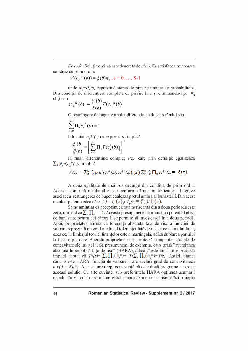
Romanian Statistical Review - Supplement nr. 2 / 201744

Dovadă. Soluția optimă este denotată de c*(z). Ea satisface următoarea condiție de prim ordin:

�����"����� ����� ������ � ������;2�3������ ���������� �����������"����������������E�

�� ,,�� �� -+--+Q+X � ��V�0�Y���(�

�

unde s=Пs/ps reprezintă starea de preț pe unitate de probabilitate. Din condiția de diferențiere completă cu privire la z și eliminându-l pe s obținem

))(*(

)(

)('))(*'( bcT

b

bbc ss ξ

ξ=

O restrângere de buget complet diferențiată aduce la rândul său

∑−

=

=Π1

0

*'1)(

S

s

ss bc

Inlocuind cs*’(z) cu expresia sa implică

���������������������((

0

Q --++-+

-+X��

���

���

���� �

!

�

�� ,��,

,

��

�

2���������������"����������� ��2�3�����������������"�������������� În fi nal, diferențiind complet v(z), care prin defi niție egalizează

su(cs*(z)), implică

2���������������"����������� ��2�3�����������������"�������������� �+� ;2�33#����������=2�3 ��=2��;2�33��;=2�3 �;=2�3

$����������� � ����������������������������"������������������$��� ���������������� � ���

A doua egalitate de mai sus decurge din condiția de prim ordin. Aceasta confi rmă rezultatul clasic conform căruia multiplicatorul Lagrage asociat cu restrângerea de buget egalează prețul umbră al bunăstării. Din acest rezultat putem vedea că v’’(z) și Tv(z) (z)/

Să ne amintim că acceptăm că rata neriscantă din a doua perioadă este zero, urmând ca Această presupunere a eliminat un potențial efect de bunăstare pentru cei cărora li se permite să investească în a doua periadă. Apoi, proprietatea afi rmă că toleranța absolută față de risc a funcției de valoare reprezintă un grad mediu al toleranței față de risc al consumului fi nal, ceea ce, în limbajul teoriei fi nanțelor este o martingală, adică dublarea pariului la fi ecare pierdere. Această proprietate ne permite să comparăm gradele de concavitate ale lui u și v. Să presupunem, de exemplu, că u arată ”aversiunea absolută hiperbolică față de risc” (HARA), adică T este liniar în c. Aceasta implică faptul că Tv(z)= s*)= T( s*)=T(z). Astfel, atunci când u este HARA, funcția de valoare v are același grad de concavitateca u:v(·) = Ku(·). Aceasta are drept consecință că cele două programe au exact aceeași soluție. Cu alte cuvinte, sub preferințele HARA opțiunea asumării riscului în viitor nu are niciun efect asupra expunerii la risc astăzi: miopia

Revista Română de Statistică - Supliment nr. 2 / 2017 45

este, în acest caz, optimă. Ceteris paribus, investitorii tineri și mai puțin tineri ar trebui să selecteze aceeași compoziție a portofoliului. Alternativ, să presupunem că funcția de utilitate u exprimă o toleranță convexă absolută față de risc. Aplicând inegalitatea Jensen, urmează că Tv(z)=

s*)= T( s*)=T(z): oportunitatea asumării riscului în viitor crește toleranța la riscurile curente. Asumarea faptului că T’’ este nonnegativ este compatibilă cu intuiția că un orizont de timp mai larg ar induce asumarea unui risc suplimentar care se regăsește în semnul celei de-a patra derivată a funcției de utilitate. Pe de altă parte, dacă T’’ este nonpozitive, un orizont de timp mai lung pentru investi’ie ar implica o investiție mai conservatoare pe termen scurt. Dacă vom presupune că rata nonriscului este zero. În problema dinamică a portofoliului Arrow-Debreu cu profi turi seriale independente, un orizont de timp mai lung ridică, respectiv reduce, expunerea optimă la risc pe termen scurt dacă toleranța absolută la risc T(·) = -u’(·)/u’’(·) este convexă, respectiv concavă. În cazul HARA,orizontul de timp nu are efect asupra portofoliului optim.

Concluzii

Atunci când investiția pe termen lung este vizată pentru consum la o dată anume, dacă investitorul ar trebui să modifi ce propria expunere la risc pe măsură ce orizontul de timp se ingustează, devine o problemă empirică bazată pe convexitate, liniaritate și concavitate a toleranței absolute față de risc. Desigur, niciuna dintre aceste condiții de toleranță absolută la risc nu trebuie menținută pentru toate nivelele de bunăstare. E posibil să existe o toleranță la risc care uneori este convexă, alteori este concavă. Pentru un asemenea individ, nu vom fi capabili să previzionăm efectul pentru un orizont de planifi care mai lung în ceea ce privește strategia investițională. În funcție de circumstanțe, acest individ va investi uneori mai mult în acțiuni, iar în alte perioade va investi mai mult în titluri de valoare care vor fi investiți în condiții de miopie investițională. Putem aprecia convexitatea/concavitatea toleranței absolute la risc prin introspecție. Să ne amintim că că, prin ecuația suma în euro optim investită în acțiuni este aproximativ proporțională cu T. Sub DARA, este vorba despre o creștere a bunăstării. Întrebarea este dacă avem de-a face cu o creștere la o rată crescătoare pe măsura creșterii bunăstării. Dacă este așa, ar fi un argument pentru un T convex și pentru un efect pozitiv al deschiderii orizontului de timp în asumarea riscului. Majoritatea modelelor teoretice fi nanciare folosesc funcțiile de utilitate HARA. În aceste modele, miopia investițională este optimă, ceea ce simplifi că mult analiza. Cineva ar putea

Romanian Statistical Review - Supplement nr. 2 / 201746

totuși suspecta că această asumare este realizată pentru a simplifi ca lucrurile,

decât pentru realismul abordării. Testele econometrice pentru preferințele

HARA sunt extrem de puține ca resurse literare de specialitate.

Bibliografi e

1. Ameur, H.B., Prigent, J.L. (2010). Behaviour towards Risk in Structured Portfolio

Management, International Journal of Economics and Finance, Vol. 2, No. 5, pp.

91-102

2. Anghel, M.G. (2013). Modele de gestiune şi analiză a portofoliilor, Editura

Economică, Bucureşti

3. Anghel, M.G. (2013). Identifi cation of fi nancial instruments – important step in

building portfolios, Romanian Statistical Review, Issue 9, pp. 52-65

4. Anghelache, C., Anghel, M.G. (2016). Econometrie generală. Concepte, teorie şi

studii de caz, Editura Artifex, Bucureşti

5. Anghelache, C., Anghel, M.G. (2015). Statistică. Teorie, concepte, indicatori şi

studii ce caz, Editura Artifex, Bucureşti

6. Anghelache, C., Anghel, M.G., Popovici, M. (2016). Model privind managementul

dinamic al portofoliului de acţiuni / Model regarding the dynamic management of

shares portfolio, Romanian Statistical Review, Supplement, no.7, pg. 79-86/87-93

7. Anghelache, C., Anghel, M.G. (2014). Using the regression model for the portfolios

analysis and management, Theoretical and Applied Economics, Volume XXI,

No.4, pp. 53-66

8. Anghelache, G.V., Anghel, M.G., Popovici, M. (2016). Signifi cant Aspects of

Investment Dynamics, Romanian Statistical Review Supplement, Issue 1/2016, pp.

68-73

9. Anghelache, G.V., Anghel, M.G. (2013). Specifi c patterns in portfolio analysis,

Theoretical and Applied Economics, Volume XX, No.11, pp. 7-24

10. Bade, Al., Frahm, G., Jaekel, U. (2009). A general approach to Bayesian portfolio

optimization, Mathematical Methods of Operations Research, v. 70, iss. 2, pp.

337-356

11. Barberis, N. (2000). Investing for the long run when returns are predictable,

Journal of Finance, 55

12. Bhalla, V.K. (2008). Investment management, Oxford University Press

13. Eeckhoudt, L., Gollier, C., Schlesinger, H. (2005). Economic and Financial

Decisions under Risk, Princeton University Press

14. Hafner, R., Wallmeier, M. (2008). Optimal investments in volatility, Financial

Markets and Portfolio Management, v. 22, issue 2

15. Malcolm, B., Taliaferro, R., Wurgler, J. (2006). Predicting Returns with

Managerial Decision Variables: Is There a Small-Sample Bias?, Journal of

Finance 61, no. 4 (2006): 1711-1730

16. Phillips, P.C.B, Sul, D. (2003). Dynamic panel estimation and homogeneity

testing under cross section dependance, Econometrics Journal, 6

Revista Română de Statistică - Supliment nr. 2 / 2017 47

THEORETICAL ASPECTS OF THE DYNAMIC PORTFOLIO MANAGEMENT

Assoc. prof. Madalina-Gabriela ANGHEL PhD.

„ARTIFEX” University of Bucharest

Assoc. prof. Mirela Panait PhD.

Petroleum-Gas University of Ploiesti, Romania

Prof. Alexandru MANOLE PhD.

„ARTIFEX” University of Bucharest

Marius POPOVICI PhD. Student

Bucharest University of Economic Studies

Abstract

Items as reverse diversifi cation, investment dynamics are subject to

this article. Investors are characterized by a longer timeframe vision concern-

ing investing activity. Corporate managers decisions focused on early gains

allows the estimation that they are strongly concerned of short-term strategy

which is considered as safe, based on sub-investment in research and develop-

ment risky projects. Taking risks on long-term investment policy might gener-

ate signifi cant advantages and benefi ts for investors, while mutual funds are

specifi cally oriented towards obtaining relevant short-term benefi ts, focusing

on long-term expectations.

Keywords: portfolio, management, dynamic decision diversifi ca-

tion

Classifi cation JEL: G 10, G 11

Introduction

Most often, investors have a long-term view on their investments. Many times, investment decisions are not reversible and we might conclude that investment management has an obvious dynamic nature. It raises the question whether investment decisions can be inferred from a static math-ematical model that can be used to defi ne a dynamic strategy. In other words, the focus is on determining the effect of investment horizon of an agent on his portfolio related risks. The usual treatment suggests that short-term time horizon often leads to excessively conservative strategy. It is well known that private companies provide a substantial benefi t from the ability they have to focus on long-term projects. It is considered that mutual fund managers fo-cus on strategies that ensure satisfactory short-term gains, without sacrifi cing long-term expectations.

Romanian Statistical Review - Supplement nr. 2 / 201748

Literature review

The fi rst to solve the problem dynamic portfolio of in a continuous time economy with HARA utility functions were Merton and Samuelson in 1969. Mossin (1968) proved that only the HARA functions consider myopia optimal when there is serial correlation of profi ts. Deaton and Carroll in the ‘90s examined the effect of liquidity constraints on the behavior of optimal savings. In 2000, Barberis estimated the predictability of signifi cant earnings produced by the US stock market. Kim and Omberg (1996) showed that the standard deviations of ten-year earnings were 23.7% lower than 45.2% of the

value implied by the standard deviation of monthly earnings, which, they said,

indicated that that happens when risk relative constant aversion is to larger

than unity. In 1999 and 2000, Campbell, Viciera and Barberis estimated that

demand for numerical coverage. The effect on profi t predictability on initial

portfolio optimal structure is surprisingly important. For an agent with relative

risk aversion equal to 10 and a ten years horizon, optimal investment in shares

represent 40% of current welfare without predictability. It rises to 100% when

the reversal of means is considered. In 1986, Detemple is the fi rst to examine

the matter of active demand under incomplete information and knowledges.

Ameur and Prigent (2010) analyzes the risky behavior in the con-

text of portfolio structured management. Anghel (2013) study portfolios man-

agement and analysis using some dedicated models. Bhalla (2008) envisages

investment management. Anghel (2013b) is concerned of identifying key role

of fi nancial instruments in portfolios management. Anghelache and Anghel

(2015, 2016) prepare reference paper regarding statistical and econometric

tools, Anghelache and Anghel (2014) described the utility model regression

analysis and portfolio management. Anghelache, Anghel and Popovici (2016)

studied the role specialized modelling in dynamic management of the shares

portfolio. Anghelache, Anghel and Popovici (2016) presented a number of

signifi cant features of the evolution of investment. Anghelache and Anghel

(2013) are concerned with identifying patterns in the analysis and portfolio

management. Bade, Frahm and Jaekel (2009) addressed Bayesian optimiza-

tion to fi nancial instruments portfolio. Eeckhoudt, Gollier and Schlesinger

(2005) analyzed the decision behavior under risk. Hafner and Wallmeier

(2008) studied volatility and its impact on optimal investment characteristics.

Malcolm, Taliaferro and Wurgler (2006) considered the variable investment

income possibility by forecasting managerial decision. Phillips and Sul (2003)

are concerned by homogeneity testing and dynamic estimation under certain

conditions.

In the fi eld of specialized literature, the issue of risk horizon and re-

ceived the highest interest by providing portfolio strategies according to agent

Revista Română de Statistică - Supliment nr. 2 / 2017 49

appropriate age. Thus, Samuelson in 1989 and still other authors addressed the question: “as you age and your investment horizon narrows, you will limit your initiatives regarding lucrative but risky share?” Conventional wisdom answers “yes!” to this question, adding that investors with a higher horizon of time can tolerate a higher risk because they have more time available to re-cover transitional losses. This argument was not supported by scientifi c theory however. As particularly Samuelson (1963, 1989) considered, the argument of “temporal diversifi cation” is based on a misinterpretation of the Law of Large Numbers. Thus, repeating a pattern investment over several periods of time does not generate risk or even beyond long periods of time. This error is illustrated by the following concerns of Samuelson on this topic in 1963. “I proposed some buddies to bet every 200 Euro to 100 Euro that the coin will not fall as they bet at the fi rst pitch. A distinguished colleague replied: “I will not bet because I feel that is 100 Euro lost is more than $ 200 won. But I bet if you promise to let me bet this 100 times. “ This story suggests that independent risks are complementary. Samuelson goes on asking why it would be best to accept separately the 100 undesirable bets. The distinguished colleague replies: “One throw is not enough to demonstrate that the law of arithmetic mean will return in my favor. But a hundred throws of the coin, the law of large numbers will turn everything in my favor. “ Obviously, this colleague of Samuelson misinterprets the Law of Large Numbers! Accepting a second chance will not reduce the risk associ-ated with the fi rst pitch. If v x̃1,x̃2, . . . , x̃n are variables of wealth distributed independently and identically and randomly, then x̃1+x̃2+ . . .+ x̃n is character-ized by n times greater of each of these risks. This is what supports the Law of Large Numbers

∑=

n

ixn 1

1

almost certainly tends to Ex̃1 as n tends to infi nity. By lowering, and adding risk, they are disappearing through diversifi cation.

2. The concept of reversing diversifi cation

Problems solving dynamic decision involve a good understanding of the method generally known as “reverse induction”. Suppose you took a se-quence of two decisions 0 in the interval 0, and 1 in the interval 1. Decision

0 concerns exposure to risk whose profi t z( 0, x) is subject to the completion of a variable x some x̃. It is important to note that x occurs after selection of

0, before the decision 1 to be made. The objective ex ante points to maximiz-ing the expectation of a function Ua of ( 0, 1, x̃):

Romanian Statistical Review - Supplement nr. 2 / 201750

++L))�� &/

&/��

��,&�� �

��

Reverse induction consists primarily in solving the problem of the second period for each possible outcome that would be prevalent at the begin-ning of that period. This set of results is complete summary of profi t z obtained in the fi rst period. The optimal strategy 1* for the second period will gener-ally depend on z, which is called dynamic variable status. This issue of the second period contingent with “z status” is written as follows:

),(max)( 11

αα

zUzv =

The optimum value of z is noted by v(z). Function v is called value function, or Bellman function. The problem the fi rst period 0 can solved by selecting risck exposure 0 that maximizes the expectation of function Ev(z(

0, x̃)). In doing so, the decision-maker internalizes the effect its future contin-gent strategy on welfare U, by v defi nition. He is “dynamic consistent”. This technique turns any dynamic problem into a sequence of static problems by the value function.

3. The signifi cance of dynamic investment

We will further examine the effect of future risk-taking opportunity on the will to assume risk on short term. In other words, an investor with a long-term planning horizon will want to invest a larger size of well-being in risky actions in opposition to safer bonds? Suppose the investor has the goal of maximizing the welfare of EU accumulated at a particular date. For example, this is the case when an investor is preparing his retirement. This money is not used for intermediate consumption. In standard terminology this is called an investment problem. Next, we introduce intermediate consumption, as we assume here the idea that while the risks are independent, a condition that will relax further. We can illustrate the problem examined in this section as follows. Starting from Samuelson’s question, suppose you are asked to bet whether a currency will fall „head” (C) or „tails” (P). Win three times your stake when the coin falls „head” (C) and loose in the opposite situation. Suppose that, given your aversion to risk, you want to bet on this single bet. Now, suppose you are told that you will allow yourself to bet sequentially in two independent throws of the coin. How will affect your bet the initial coin toss? This question is equivalent to the time horizon of the investor’s optimal portfolio composition. Consider the following more general problem. An investor with wealth experiences two periods. At the beginning of each period, he has the

Revista Română de Statistică - Supliment nr. 2 / 2017 51

opportunity to take some risk whose accomplishment will be visible at the end of that period. It is important to observe that the investor will become aware of the loss or gain arising from the risk assumed in the fi rst period before decid-ing to measure the risk he assumed in the second period. This will make the problem inherently dynamic and it will some fl exibility which is essential for

dynamic risk management. To illustrate, under DARA conditions, investors

will assume less risk in the second period in case they suffered major portfolio

losses in the fi rst period. To be precise, suppose that the problem of the two periods is a decision Arrow-Debreu portfolio. There are s of the nature state

s=0, ... , S-1 . The uncertainty prevailing in the second period is characterized by the vector of probabilities (p0,…, ps-1 ). Пs is the unit price of Arrow-De-

breu security associated to state s. Let us uppose the un-risky rate is zero. This

implies that a claim has a value of 1 leu for each natural state must itself cost

1 leu; ΣsΠs = 1. In other words if an investor assumes the risk in the second

period he will end up with the same fi nal welfare as in the fi rst period. Given welfare b being accumulated at the end of the fi rst period, the investor selects a portfolio (c0, ... , cs-1) that maximizes the EU’s welfare at the end of which is subject to restriction:

)(max)(

1

0,..., 10

∑−

=−

=S

s

sscc

cupzvs

is subject to restrictions bcS

s

ss =Π∑−

=

1

0

This is equivalent to the problem indicated by the equation, and

∑∑ −

=

−

= +

Π

Π−=

1

10

1

101 )(),(

S

s

ss

S

s

ss

cup

cb

upzU α

During zero period of time, investor must take a decision involving a profi t z(0, x) depending on the attainment of a variable x. In particular, this could be another problem of portfolio choice. The optimum exposure to risk during the period 0 is obtained by accomplishing the following schedule:

++L))�� ��� /

/

M

/ ,#�� ���

�

L

�

We aim to determine the impact of risk-taking opportunity in the second period in connection with the exposure in the fi rst period. To achieve this, we compare the obtained solution 0* within a dynamic program with optimal exposure to risk in the fi rst period, when there is no option to take risks in the second period. Investor with short life, like the shortsighted would select the level that would maximize EU for z( 0, x̃):

Romanian Statistical Review - Supplement nr. 2 / 201752

++L))�� ���S

//

/ ,#�� ���

��

� @������� ���� �����������������������������������

�

. We see that the only difference between programs consists in the fact that utility function u in the fi rst program replaces the function of the second value v. This can be expressed by saying that the future effect is com-pletely captured by the characteristics of the value function. In the present context, risk taking opportunity in the future increases the willingness to take risks today if v is less concave than u as Arrow-Platt assesses. The optimum exposure to risk in the fi rst period is greater than the myopic exposure operated if the value function v defi ned as less concave than the original utility function u, for instance v is more risk tolerant than u. The degree of absolute risk tolerance v is characterized by the news of his sen-tence. Value function for the problem of portfolio Arrow Platt (& .3) has a

high absolute risk tolerance given in equation

� �+�����������' ���� ���:��� ���

��

�

���&

/

M+)

+)NN

+)N+)

!

�

�� ��#�

#�#��

�

�

where c * is the optimal solution to the problem and T (·)= -u’(·)/u’’(·)

represents the absolute risk tolerance for fi nal consumption.

Proof. The optimal solution is denoted by c * (z). It satisfi es the fol-lowing fi rst order condition:

�� ##�� �� +)++)M)N � ���R�/�T�%�&�

�

where s=Пs/ps is the state price per unit of probability. From the condition of complete differentiation on z and eliminatings, we have

�������������������������&�������������������� ����

++)M)+)

+)N++)MN) #��

#

##� �� �

��

� A full differentiated limitation on the budget brings

∑−

=

=Π1

0

*' 1)(S

s

ss bc

Replacing cs*’(z) the expression implies

&&

/

M ++))+)

+)N��

���

���

���� �

!

�

�� #��#

#

��

�

Finally, the fully differentiating v(z), which by defi nition equalizes

su(cs*(z)), involves

Revista Română de Statistică - Supliment nr. 2 / 2017 53

� �

�=1&2��� ����� ��=1��;1&22��;=1&2 ���� � ��

���� �;=1&2� � �����

A second equality above stems from the condition of fi rst order. This result confi rms that the classic Lagrage multiplier associated with budget restriction equals the shadow price of welfare. From this result we can see that 3�����������1&2� )&2>� 3������

� � � ��

Let us remember that we accept that the rate of un-risky second period is zero, following that

� � ����

�G������ ��������� � ������ ������� � ��� � �� ����� ��� ��

���������� ����� � � ���� �� �� ������������ �����������������������������

�������� ���� � ���� � �� ���� �������� ��� ������ �� � ��

. This has removed the assumption of a potential effect of welfare for those who are allowed to invest in the second period. Then, this property states that absolute risk tolerance against value function is an average degree of fi nal consumption risk tolerance, which, in the language of fi nances is a martingale theory, ie doubling the bet every loss. This property enables us to compare the degree of concavity of u and v. Suppose, for example, that u shows „ absolute hyperbolic aversion to risk” (HARA) that is that T is linear in c. This implies that

��������� ��������� �������� ��� ���B� )"#$#+� � ���

������ � ��� ��1&24�� � ���� �;24� �1� � ���� �;24�1&2%� � ��� � ��

�������������� ��� � �������������������������� ��

. Thus, when u is HARA, the value function has the same degree of concavity like u:v(·) = Ku(·). This has the con sequence that the two programs have exactly the same solution. In other words, under HARA preferences, the option of risk taking in the future has no effect on risk exposure today: in this case, myopia is optimum.Ceteris paribus, young and less young investors should select the same composition of the portfolio. Alternatively, assume that the utility function u expresses a con-vex absolute tolerance for risk. Applying the Jensen inequality, it follows that ��1&24�� � ���� �;24� �1� � ���� �;24�1&2-�

��������� ���������� ������� �������� ������ #������

risk taking opportunity in the future increases tolerance against current risks. Assuming that T’’ is non-negative is compatible with the intuition that a wider time horizon would induce addi-tional risk taking that is found in the sign of the fourth derivative of the utility function. On the other hand, if T’ is non-positive, a longer time horizon for investment might suppose a more conservative investment in the short term. Assuming a zero non-risk rate, concerning Arrow-Debreu portfolio dynamics with independent serial profi ts, a longer time horizon raises or re-duces the optimal exposure to risk in the short term if the absolute risk toler-ance T(·)=-u’(·)/u’’(·) is convex or concave. Under HARA, the time horizon has no effect on the optimum portfolio.

Conclusions

When long-term investment is targeted for consumption at a given date, if the investor should amend its exposure to risk as the time horizon nar-rows, it becomes an empirical issue based on convexity, linearity and concav-ity tolerance absolute to risk. Of course, none of these conditions of absolute

Romanian Statistical Review - Supplement nr. 2 / 201754

risk tolerance should be applied to all levels of welfare. It may be a risk toler-ance that is sometimes convex, sometimes concave. For such an individual will not be able to predict the effect of a longer planning horizon regarding in-vestment strategy. Depending on the circumstances, this individual will some-times invest more in shares and in other periods will invest more in securities that will be invested in myopic investment conditions. We might appreciate convexity/concavity of absolute risk tolerance by introspection. Let us remember that that equation in euro optimal amount invested in shares is approximately proportional to T. Under DARA, we have welfare gains. The question is whether we are dealing with an increase at an increasing rate with the wealth increasing. If so, it would be an argument for T convex and a positive effect of opening time horizon in risk taking. Most theoretical models use fi nancial utility functions HARA. In these models, in-vestment myopia is optimal, which greatly simplifi es the analysis. One might suspect, however, that this assumption is made to simplify things, than for a realist approach. HARA preferences econometric tests are extremely scanty literature resources.

Bibliografi e

1. Ameur, H.B., Prigent, J.L. (2010). Behaviour towards Risk in Structured Portfolio

Management, International Journal of Economics and Finance, Vol. 2, No. 5, pp. 91-102

2. Anghel, M.G. (2013). Modele de gestiune şi analiză a portofoliilor, Editura Economică, Bucureşti

3. Anghel, M.G. (2013). Identifi cation of fi nancial instruments – important step in

building portfolios, Romanian Statistical Review, Issue 9, pp. 52-65 4. Anghelache, C., Anghel, M.G. (2016). Econometrie generală. Concepte, teorie şi

studii de caz, Editura Artifex, Bucureşti 5. Anghelache, C., Anghel, M.G. (2015). Statistică. Teorie, concepte, indicatori şi

studii ce caz, Editura Artifex, Bucureşti 6. Anghelache, C., Anghel, M.G., Popovici, M. (2016). Model privind managementul

dinamic al portofoliului de acţiuni / Model regarding the dynamic management of shares portfolio, Romanian Statistical Review, Supplement, no.7, pg. 79-86/87-93

7. Anghelache, C., Anghel, M.G. (2014). Using the regression model for the portfolios analysis and management, Theoretical and Applied Economics, Volume XXI, No.4, pp. 53-66

8. Anghelache, G.V., Anghel, M.G., Popovici, M. (2016). Signifi cant Aspects of Investment

Dynamics, Romanian Statistical Review Supplement, Issue 1/2016, pp. 68-73 9. Anghelache, G.V., Anghel, M.G. (2013). Specifi c patterns in portfolio analysis,

Theoretical and Applied Economics, Volume XX, No.11, pp. 7-24 10. Bade, Al., Frahm, G., Jaekel, U. (2009). A general approach to Bayesian portfolio

optimization, Mathematical Methods of Operations Research, v. 70, iss. 2, pp. 337-356 11. Barberis, N. (2000). Investing for the long run when returns are predictable,

Journal of Finance, 55

Revista Română de Statistică - Supliment nr. 2 / 2017 55

12. Bhalla, V.K. (2008). Investment management, Oxford University Press 13. Eeckhoudt, L., Gollier, C., Schlesinger, H. (2005). Economic and Financial

Decisions under Risk, Princeton University Press 14. Hafner, R., Wallmeier, M. (2008). Optimal investments in volatility, Financial

Markets and Portfolio Management, v. 22, issue 2 15. Malcolm, B., Taliaferro, R., Wurgler, J. (2006). Predicting Returns with

Managerial Decision Variables: Is There a Small-Sample Bias?, Journal of Finance 61, no. 4 (2006): 1711-1730

16. Phillips, P.C.B, Sul, D. (2003). Dynamic panel estimation and homogeneity

testing under cross section dependance, Econometrics Journal, 6

Romanian Statistical Review - Supplement nr. 2 / 201756

Diversifi carea temporală în consum şi economisire

Prof. univ. dr. Constantin ANGHELACHE

Academia de Studii Economice București, Universitatea „ARTIFEX” București

Prof. univ. dr. Radu Titus MARINESCU

Universitatea „ARTIFEX” București

Asistent univ dr. Diana Valentina DUMITRESCU

Universitatea „ARTIFEX” din București

Abstract

Conceptul portofoliului dinamic s-a impus în literatura de

specialitate odată cu extinderea orizontului temporal al analizei și modelării comportamentului investițional. Astfel, ieșind din lipsa de defi niție pe care analiza statică a impus-o rezultatului alegerii agentului, extinderea orizontului temporal și implicarea acestuia ca factor dinamic activ în procesele deciziei investiționale au sporit șansele unei analize cât mai amănunțite și ale

unei modelări cât mai fi dele a proceselor psihologice subîntinse deciziei

individuale.

Cuvinte cheie: diversifi care, risc, consum, toleranţă, predicţie

Clasifi care JEL: G10, G11

Introducere

În context investițional, se precizează o dată de consum unică. Aceasta implică faptul că toate riscurile asumate de-a lungul vieții s-au generat la acea dată. În cele mai multe situații, investitorii vor dori să utilizeze portofoliile proprii pentru a fi nanța consumul de-a lungul vieții. Evident, acest model

este mult simplifi cat. De exemplu, stimulentele din impozite reale pot lucra

împotriva acestei posibilități. Această situație prezintă un important avantaj,

de alocare a riscurilor curente privitoare la bunăstare în riscuri mai mărunte

privind un orizont larg al consumului. Aceasta produce un important efect de

diversifi care în timp, ceea ce îi determină pe cei cu un orizont al planifi cării

mai extins să își asume mai multe riscuri.

Literature review

Dacă consumatorii nu pot împrumuta bani atunci când există un șoc

temporar negativ asupra veniturilor lor ei vor fi mult mai dornici să acumuleze

bunăstare ex ante. Acest depozit tampon conduce la un nou motiv de a economisi

(Deaton 1991; Carroll 1997). Anghelache, Anghel şi Manole (2015) descriu

instrumentele modelării pentru domeniul economic. Anghelache, Anghel

Revista Română de Statistică - Supliment nr. 2 / 2017 57

şi Popovici (2015) aplică regresia multiplă în analiza consumului public şi privat, Anghelache, Soare şi Popovici (2015) evaluează infl uenţa consumului fi nal asupra evoluţiei Produsului Intern Brut al României, o analiză a aceluiaşi indicator macroeconomic este realizată de Anghelache, Manole şi Anghel (2015). Anghelache, (2008), Anghelache, Mitruţ şi Voineagu (2013) se preocupă de măsurarea indicatorilor macroeconomici, Anghelache şi Voineagu (2009), Anghelache, Anghelache şi Bădulescu (2008), Ghysels şi Osborn (2001) studiază seriile de timp. Hribar şi McInnis (2012) analizează erorile de previzionare a benefi ciilor asociate investiţiilor. Kalaman şi Zhalinska (2012) descriu rolul fondurilor de investiţii în fi nanţarea inovării. Ravi et.al. (2014) se preocupă de corelaţia între volatilitate şi preţurile activelor.

Aspecte generale privind diversifi carea temporală

Pentru a explica aceasta, să considerăm un model mai simplu în care agentul are ocazia să își asume un risc la data t = -1. Mai detaliat, presupunem că profi tul pentru jocul asumării riscului inițial z( 0, x̃), unde 0 reprezintă o variabilă decizională, iar x̃ este o variabilă oarecare. În continuare, agentul consumă pe durata perioadelor rămase n, numerotate t = 0, . . . , n – 1. Să presupunem că agentul poate economisi sau împrumuta cu o rată a dobânzii zero, și că el nu are ocazii să își asume riscuri începând cu data t = 0. Mai mult, în fi ecare peroadă el câștigă un venit y din muncă. Această problemă indică aceeași structură dinamică prezentată în secțiunea 7.1. Pentru a determina expunerea optimă la risc în prima perioadă, este nevoie să rezolvăm mai întâiproblema consum- economisire după ce efectul riscant este indicat. Pentru o bunăstare dată z acumulată anterior datei t = 0, putem nota

∑−

=

=1

0

)(max)(n

ttt

ccupbv supus restrictiei

�

�����������������

�

��$

.

�

�4+� �

unde pt este un factor de reducere asociat datei t, iar z + ny este bunăstarea la nivelul întregii vieți. Cu această funcție de valoare v , se poate determina nivelul optim al asumării toleranței la riscul inițial relativ la funcția valorică v. Așa cum observam mai înainte, structura problemei consum – economisire este esențial aceeași ca problema portofoliului Arrow – Debreu din Propoziția &.1. Principala diferență constă în faptul că nu dispunem de prețuri de stare, astfel că trebuie să presupunem că pentru toți s. Din propoziția de mai sus, deducem:

��

�

�$

.

F )#)#�

��+�� �

Romanian Statistical Review - Supplement nr. 2 / 201758

unde ct* reprezintă soluția optimă a problemei. În problema raportului cert dintre consum și economisirepentru datele t = 0, n – 1 cu rata a dobânzii zero, gradul de toleranță față de risc la bunăstarea inițială egalează suma toleranțelor absolute față de riscul în consumde-a lungul vieții consumatorului. Vom examina în continuare efectul unei creșteri în n asupra lui Tv(z).

Pentru simplifi care, să presupunem că consumatorii nu sunt nerăbdători, astfel că pt = 1 pentru toți t. Astfel, este optim să calmezi complet consumul:ct* =

y + (z/n) la fi ecare dată t. În acest aranjament, toate câștigurile și pierderile asumate la primul risc sunt alocate egal de-a lungul perioadelor de consum n

rămase.Proprietatea poate fi scrisă sub forma:

��

��

��+

�4��+�� )# �

Pentru un risc inițial mic (z mic), toleranța absolută la risc relativ la bunăstare este proporțională cu durata vieții jucătorului. Astfel, un agent care așteaptă să trăiască de două ori mai mult decât un alt agent cu același venit anual, poate investi aproximativ de două ori mai mult în acțiuni decât celălalt la data t = 1. Acesta este sensul real care ar trebui acordat noțiunii de ”diversifi care temporală”. Desigur, presupunem că există doar un singur punct în timp cînd consumatorii își asumă riscul. În lumea reală, consumatorii pot deține acțiuni și își pot suma riscuri în orice moment. Această presupunere mult mai realistă nu va schimba rezultatul obținut anterior în cazul HARA.Într-adevăr, utilizând inducția inversă, adăugînd soluţia de asumare a riscului în viitor nu s-ar schimba concavitatea funcției valorice la o dată oarecare atunci când HARA este presupusă. Agenții sunt absenţi față de riscurile viitoare în acest caz, iar proprietatea anterioară încă se susține. O altă evaluare într-un fundal mai realist o reprezintă existența restrângerilor de bani lichizi. Diversifi carea temporală operează bine numai în situația în care consumatorii pot împrumuta bani cu o dobândă acceptabilă atunci când sunt confruntați cu un șoc advers asupra veniturilor proprii și când rezervele lor bănești sunt epuizate. Aceasta este o presupunere nerealistă. Agenții care nu dispun de lichidități, nu pot face față unui șoc negativ asupra veniturilor împrumutând bani de la banca lor. Ei nu pot recurge la o diversifi care temporală completă. Asemenea restrângeri fi nnciare implică sitația în care agenții ar trebui să aibă o aversiune mai mare față de riscuri. Acesta este un argument suplimentar în favoarea descreșterii absolute a aversiunii față de risc.

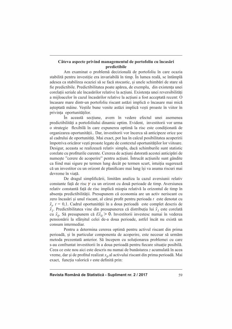
Revista Română de Statistică - Supliment nr. 2 / 2017 59

Câteva aspecte privind managementul de portofoliu cu încasări

predictibile Am examinat o problemă decizională de portofoliu în care ocazia stabilită pentru investiție era invariabilă în timp. În lumea reală, se întâmplă adesea ca stabilirea ocaziei să se facă stocastic, și unele schimbări de stare să fi e predictibile. Predictibilitatea poate apărea, de exemplu, din existența unei corelații seriale ale încasărilor relative la acțiuni. Existența unei reversibilități a mijloacelor în cazul încasărilor relative la acțiuni a fost acceptată recent: O încasare mare dintr-un portofoliu riscant astăzi implică o încasare mai mică așteptată mâine. Veștile bune venite astăzi implică vești proaste în viitor în privința oportunităților. În această secțiune, avem în vedere efectul unei asemenea predictibilități a portofoliului dinamic optim. Evident, investitorii vor urma o strategie fl exibilă în care expunerea optimă la risc este condiționată de organizarea oportunității.. Dar, investitorii vor încerca să anticipeze orice șoc al cadrului de oportunități. Mai exact, pot lua în calcul posibilitatea acoperirii împotriva oricăror vești proaste legate de contextul oportunităților lor viitoare. Desigur, aceasta se realizează relativ simplu, dacă schimburile sunt statistic corelate cu profi turile curente. Cererea de acțiuni datorată acestei anticipări de numește ”cerere de acoperire” pentru acțiuni. Întrucât acțiunile sunt gândite ca fi ind mai sigure pe termen lung decât pe termen scurt, intuiția sugerează că un investitor cu un orizont de planifi care mai lung își va asuma riscuri mai devreme în viață. De dragul simplifi cării, limităm analiza la cazul aversiunii relativ constante față de risc cu un orizont cu două perioade de timp. Aversiunea relativ constantă față de risc implică miopia relativă la orizontul de timp în absența predictibilității. Presupunem că economia are un activ neriscant cu zero încasări și unul riscant, al cărui profi t pentru perioada t este denotat cu x̃t, t = 0,1. Cadrul oportunității în a doua perioadă este complet descris de x̃1. Predictibilitatea vine din presupunerea că distribuția lui x̃1 este corelată cu x̃0. Să presupunem că Ex̃0 Investitorii investesc numai în vederea pensionării la sfârșitul celei de-a doua perioade, astfel încât nu există un consum intermediar. Pentru a determina cererea optimă pentru activul riscant din prima perioadă, și în particular componenta de acoperire, este necesar să urmăm metoda prezentată anterior. Să începem cu soluţionarea problemei cu care s-au confruntat investitorii în a doua perioadă pentru fi ecare situație posibilă. Ceea ce este nou aici este descris nu numai de bunăstarea z acumulată în acea vreme, dar și de profi tul realizat x0 al activului riscant din prima perioadă. Mai exact, funcția valorică v este defi nită prin:

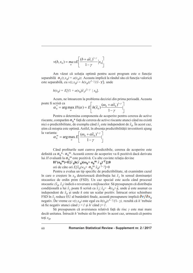
Romanian Statistical Review - Supplement nr. 2 / 201760

�

��

��

�

�

��

�

.

$

$.

$

)H#)�# #

#�+#���#+�

�

�

�

H

H

Am văzut că soluția optimă pentru acest program este o funcție separabilă 1(z,x0) = a(x0)z. Aceasta implică la rândul său că funcția valorică este separabilă, cu v(z,x0) = h(x0)z1- γ/(1- , unde

h(x0) = E[(1 + a(x0)x̃1)1- γ | x0].

Acum, ne întoarcem la problema deciziei din prima perioadă. Aceasta poate fi scrisă ca

−

+==

−

γαω

ααγ

α 1

)~()~()(maxarg

100

0*0

xxhEH

Pentru a determina componenta de acoperire pentru cererea de active riscante, comparăm 0* față de cererea de active riscante atunci când nu există nici o predictibilitate, de exemplu când x̃1 este independent de x̃0. În acest caz, știm că miopia este optimă. Astfel, în absența predictibilității investitorii ajung la varianta:

−

+=

−

γαω

αγ

α 1

)~(maxarg

100

0

xEm

Când profi turile sunt cumva predictibile, cererea de acoperire este

defi nită ca 0*- 0m. Această cerere de acoperire va fi pozitivă dacă derivata

lui H evaluată la 0m este pozitivă. Cu alte cuvinte relaţia devine

H’(α0m)=E[x̃ 0h(x̃ 0)(ω0+ α0

m x̃ 0)-ϒ]≥0

ori de câte ori E[x̃0(w0+ 0m x̃0) 1- γ]=0

Pentru a evalua un tip specifi c de predictibilitate, să examinăm cazul în care o creștere în x0 deteriorează distribuția lui x̃1 în sensul dominanței stocastice de ordin prim (FSD). Un caz special este acela când procesul stocastic (x̃0, x̃1) indică o reversare a mijloacelor. Să presupunem că distribuția condițională a lui x̃1 poate fi scrisă ca x̃1| x̃0= - x0+ , unde este asumat ca independent de x̃0 și unde k este un scalar pozitiv. Întrucat orice schimbare FSD în x̃1 reduce EU al bunăstării fi nale, această presupunere implică 0 negativ. De vreme ce v(z,x0) este egal cu h(x0)z1- γ/(1- γ), rezultă că h’ trebuie să fi e negativ atunci când γ <1 și h’ când γ>1. Să presupunem că aversiunea relativă față de risc γ este mai mare decât unitatea. Întrucât h’ trebuie să fi e pozitiv în acest caz, urmează că pentru toți x0,

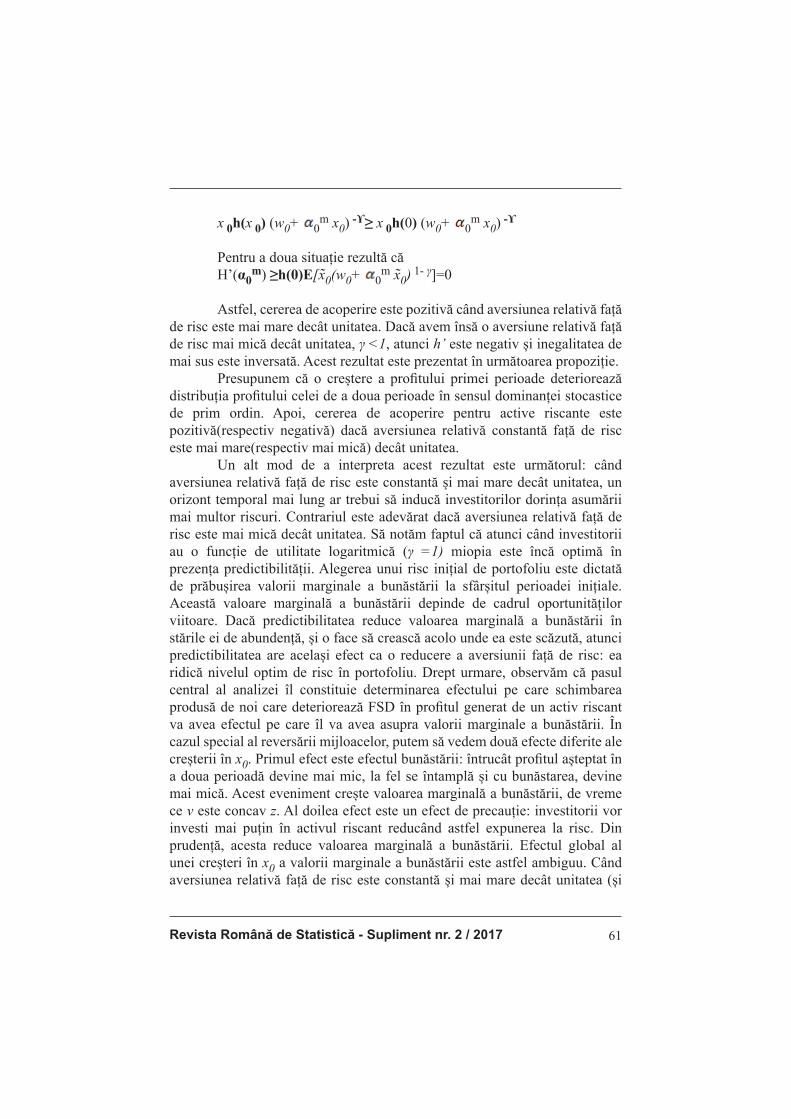
Revista Română de Statistică - Supliment nr. 2 / 2017 61

x 0h(x 0) (w0+ 0m x0) -ϒ≥ x 0h(0) (w0+ 0

m x0) -ϒ

Pentru a doua situație rezultă că

H’(α0m) ≥h(0)E[x̃0(w0+ 0

m x̃0) 1- γ]=0

Astfel, cererea de acoperire este pozitivă când aversiunea relativă față

de risc este mai mare decât unitatea. Dacă avem însă o aversiune relativă față

de risc mai mică decât unitatea, γ <1, atunci h’ este negativ și inegalitatea de mai sus este inversată. Acest rezultat este prezentat în următoarea propoziție.

Presupunem că o creștere a profi tului primei perioade deteriorează distribuția profi tului celei de a doua perioade în sensul dominanței stocastice de prim ordin. Apoi, cererea de acoperire pentru active riscante este pozitivă(respectiv negativă) dacă aversiunea relativă constantă față de risc este mai mare(respectiv mai mică) decât unitatea. Un alt mod de a interpreta acest rezultat este următorul: când aversiunea relativă față de risc este constantă și mai mare decât unitatea, un orizont temporal mai lung ar trebui să inducă investitorilor dorința asumării mai multor riscuri. Contrariul este adevărat dacă aversiunea relativă față de risc este mai mică decât unitatea. Să notăm faptul că atunci când investitorii au o funcție de utilitate logaritmică (γ =1) miopia este încă optimă în prezența predictibilității. Alegerea unui risc inițial de portofoliu este dictată de prăbușirea valorii marginale a bunăstării la sfârșitul perioadei inițiale. Această valoare marginală a bunăstării depinde de cadrul oportunităților viitoare. Dacă predictibilitatea reduce valoarea marginală a bunăstării în stările ei de abundență, și o face să crească acolo unde ea este scăzută, atunci predictibilitatea are același efect ca o reducere a aversiunii față de risc: ea ridică nivelul optim de risc în portofoliu. Drept urmare, observăm că pasul central al analizei îl constituie determinarea efectului pe care schimbarea produsă de noi care deteriorează FSD în profi tul generat de un activ riscant va avea efectul pe care îl va avea asupra valorii marginale a bunăstării. În cazul special al reversării mijloacelor, putem să vedem două efecte diferite ale creșterii în x0. Primul efect este efectul bunăstării: întrucât profi tul așteptat în a doua perioadă devine mai mic, la fel se întamplă și cu bunăstarea, devine mai mică. Acest eveniment crește valoarea marginală a bunăstării, de vreme ce v este concav z. Al doilea efect este un efect de precauție: investitorii vor investi mai puțin în activul riscant reducând astfel expunerea la risc. Din prudență, acesta reduce valoarea marginală a bunăstării. Efectul global al unei creșteri în x0 a valorii marginale a bunăstării este astfel ambiguu. Când aversiunea relativă față de risc este constantă și mai mare decât unitatea (și

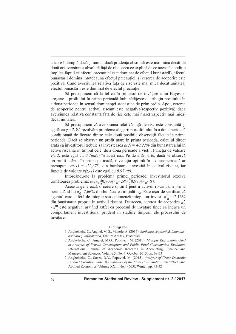
Romanian Statistical Review - Supplement nr. 2 / 201762

asta se întamplă dacă și numai dacă prudența absolută este mai mica decât de două ori aversiunea absolută față de risc, ceea ce explică de ce această condiție implică faptul că efectul precauției este dominat de efectul bunăstării), efectul bunăstării domină întotdeauna efectul precauției, și cererea de acoperire este pozitivă. Când aversiunea relativă față de risc este mai mică decât unitatea, efectul bunăstării este dominat de efectul precauției. Să presupunem că la fel ca în procesul de învățare a lui Bayes, o creștere a profi tului în prima perioadă îmbunătățește distribuția profi tului în a doua perioadă în sensul dominanței stocastice de prim ordin. Apoi, cererea de acoperire pentru activul riscant este negativă(respectiv pozitivă) dacă aversiunea relativă constantă față de risc este mai mare(respectiv mai mică) decât unitatea. Să presupunem că aversiunea relativă față de risc este constantă și egală cu γ =2. Să rezolvăm problema alegerii portofoliului în a doua perioadă condiționată de fi ecare dintre cele două posibile observații făcute în prima perioadă. Dacă se observă un profi t mare în prima perioadă, calculul direct arată că investitorul trebuie să investească a(2) = 40,22% din bunăstarea lui în active riscante în timpul celei de a doua perioade a vieții. Funcția de valoare v(z,2) este egal cu 0,76u(z) în acest caz. Pe de altă parte, dacă se observă un profi t scăzut în prima perioadă, investiția optimă în a doua perioadă ar presupune a(-1) = -12,67% din bunăstarea investită în activul riscant, iar funcția de valoare v(z,-1) este egal cu 0,97u(z).

Întorcându-ne la problema primei perioade, investitorul rezolvă următoarea problemă: 0,76u(w0+2 + 0,97u(w0- ).

Aceasta generează o cerere optimă pentru activul riscant din prima perioadă al lui =7,66% din bunăstarea inițială w0. Este ușor de verifi cat că agentul care suferă de miopie sau acționează miopic ar investi =12,13% din bunăstarea proprie în activul riscant. De aceea, cererea de acoperire - este negativă, arătând astfel că procesul de învățare tinde să inducă un comportament investițional prudent în stadiile timpurii ale procesului de învățare.

Bibliografi e

1. Anghelache, C., Anghel, M.G., Manole, A. (2015). Modelare economică, fi nanciar-bancară şi informatică, Editura Artifex, Bucureşti

2. Anghelache, C., Anghel, M.G., Popovici, M. (2015). Multiple Regressions Used in Analysis of Private Consumption and Public Final Consumption Evolution, International Journal of Academic Research in Accounting, Finance and Management Sciences, Volume 5, No. 4, October 2015, pp. 69-73

3. Anghelache, C., Soare, D.V., Popovici, M. (2015). Analysis of Gross Domestic Product Evolution under the Infl uence of the Final Consumption, Theoretical and Applied Economics, Volume XXII, No.4 (605), Winter, pp. 45-52

Revista Română de Statistică - Supliment nr. 2 / 2017 63

4. Anghelache, C., Manole, A., Anghel, M.G. (2015). The analysis of the correlation

between GDP, private and public consumption through multiple regression, Romanian Statistical Review - Supplement, No. 8, pp. 34 – 40

5. Anghelache, C., Mitruţ, C., Voineagu, V. (2013). Statistică macroeconomică. Sistemul Conturilor Naţionale, Editura Economică, Bucureşti

6. Anghelache, C., Voineagu, V. (2009). Seriile de timp utilizate ca traiectorii ale proceselor stocastice, Simpozion naţional „Management şi performanţă

economică”, Editura Artifex, pp. 207-214

7. Anghelache, C. (2008). Tratat de statistică teoretică şi economică, Editura

Economică, Bucureşti

8. Anghelache, C., Anghelache, G.V., Bădulescu, M. (2008). Analiza seriilor de timp prin utilizarea metodei spectrale, Revista Română de Statistică Supliment, nr. 3,

pp. 10-26

9. Carroll, C.D. (1997). Buffer-stock saving and the life cycle/permanent income hypothesos, Quarterly Jornal of Economics, 112

10. Deaton, A. (1991). Saving and liquidity constraints, Econometrica, 59

11. Ghysels, E., Osborn, D. (2001). The Econometric Analysis of Seasonal Time Series, Cambridge University Press

12. Hribar, P., McInnis, J. (2012). Investor Sentiment and Analysts’ Earnings Forecast Errors, Management Science 58, no. 2, pg. 293-307

13. Kalaman, O., Zhalinska, O. (2012). Venture capital as a major source of investment in innovation, Journal of Applied Management and Investments,

Volume (Year): 1 (2012), Issue (Month): 1 (), pp. 92-98

14. Ravi, B., Kiku, D., Shaliastovich, I., Yaron, A. (2014). Volatility, the Macroeconomy, and Asset Prices, Journal of Finance 69, no. 6, pg. 2471-2511

Romanian Statistical Review - Supplement nr. 2 / 201764

TIME DIVERSIFICATION IN CONSUMPTION AND SAVING

Prof. Constantin ANGHELACHE PhD.

Bucharest University of Economic Studies, „ARTIFEX” University of Bucharest

Prof. Radu Titus MARINESCU PhD.

„ARTIFEX” University of Bucharest

Assist. prof. Diana Valentina DUMITRESCU PhD.

„ARTIFEX” University of Bucharest

Abstract

The concept of dynamic portfolio was imposed in literature with

the expansion of the time horizon analysis and of the investment behavior

modeling. Thus, coming out of scope defi nition that static analysis has

imposed to the agent election outcome, the time horizon expansion and its

involvement as an active dynamic factor into the decision of investment

processes increased the chances of a thorough analysis as of a more accurate

modeling of psychological processes related to individual decision.

Key words: diversifi cation, risk, consume, tolerance, prediction

JEL clasifi cation: G10, G11

Introduction

In the investment context, it is specifi ed a unique moment of consumption. This implies that all risks of lifetime were generated at that moment. In most cases, investors will want to use their own portfolios to fi nance their consumption throughout life. Obviously, this model is much simplifi ed. For example, actual tax incentives may work against this possibility. This situation presents a major advantage for the allocation of current risks relating to the risks lesser welfare on a wider horizon of consumption. This produces an important diversifi cation effect over time, which leads those with a broader horizon planning to take more risks.

Literature review

If consumers can not borrow money when there is a temporary negative impact on their income they will be more willing to accumulate ex

ante wealth. This buffer deposit leads to another reason to save (Deaton 1991; Carroll 1997). Anghelache, Anghel and Manole (2015) describe the tools for economic modeling. Anghelache, Anghel and Popovici (2015) apply multiple regression analysis for private and public consumption, Anghelache, Sun and Popovici (2015) evaluated the infl uence of fi nal consumption on GDP evolution in Romania, an analysis of the same macroeconomic indicator is performed

Revista Română de Statistică - Supliment nr. 2 / 2017 65

by Anghelache, Manole and Anghel (2015). Anghelache, (2008), Anghelache, Mitruţ and Voineagu (2013) are concerned with the macroeconomic indicators

measurement, Anghelache and Voineagu (2009), Anghelache, Anghelache and

Bădulescu (2008), Ghysels and Osborn (2001) studied the time series. Hribar

and McInnis (2012) examin the forecasting errors of benefi ts associated to investment. Kalaman and Zhalinska (2012) describe the role of investment funds in fi nancing innovation. Ravi et.al. (2014) is concerned with the

correlation between volatility and asset prices.

General apects regarding time diversifi cation

To explain this, we will consider a simpler model where the agent has

the opportunity to take a risk on the moment t 1. In detail, we assume that

the profi t of the initial game risk assumption z( 0, x̃), where 0 represents

a decision variable and x̃ an ordinary variable. Next, the agent uses in the

remaining periods n, numbered t = 0, . . . , n – 1. Assuming that the agent can

save or borrow with a zero interest rate, and that he has no opportunity to take

risks starting with t = 0. Moreover, every time he earns from employment an

income y. This issue shows the same dynamic structure presented in Section

7.1. To determine optimal exposure to risk in the fi rst period, we need to solve

fi rstly the consum-saving issue after after the risky effect is shown. For a given

wealth z accumulated prior to t = 0, we can note

∑−

=

=1

0

)(max)(n

ttt

ccupbv subject to restrictions

�

�����������������

�

��$

.

�

�4+� �

where pt is a reduction factor associated to the moment t, and z + ny

it is is the welfare of the entire lives. With this function of value v , it can be

determined the optimal level of assumption of risk tolerance relative to the

original value function v. As we noted above, the structure of consumption – saving problem is

essentially the same as the Arrow – Debreu problem of Proposition & .1. The main difference is that prices do not have a status, so we must assume that

for all s. From the above sentence, we deduce:

��

�

�$

.

F )#)#�

��+�� �

where ct* is the optimal solution to the problem. In the problem of certain relation between consumption and saving for t = 0, n – 1 with zero interest rate, the degree of tolerance to risk the at the initial welfare equals the sum of absolute tolerances to risk in consumption over the life of the consumer.

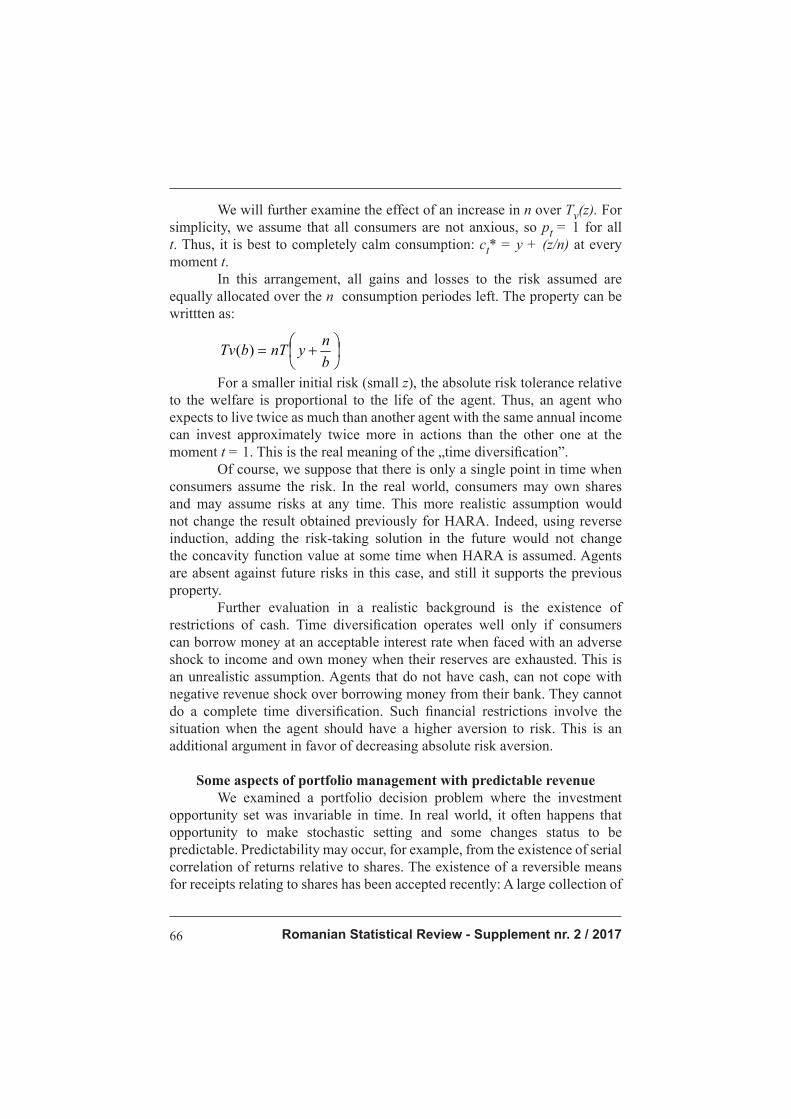
Romanian Statistical Review - Supplement nr. 2 / 201766

We will further examine the effect of an increase in n over Tv(z). For simplicity, we assume that all consumers are not anxious, so pt = 1 for all t. Thus, it is best to completely calm consumption: ct* = y + (z/n) at every moment t. In this arrangement, all gains and losses to the risk assumed are equally allocated over the n consumption periodes left. The property can be writtten as:

��

��

��+

�4��+�� )# �

For a smaller initial risk (small z), the absolute risk tolerance relative to the welfare is proportional to the life of the agent. Thus, an agent who expects to live twice as much than another agent with the same annual income can invest approximately twice more in actions than the other one at the moment t = 1. This is the real meaning of the „time diversifi cation”. Of course, we suppose that there is only a single point in time when consumers assume the risk. In the real world, consumers may own shares and may assume risks at any time. This more realistic assumption would not change the result obtained previously for HARA. Indeed, using reverse induction, adding the risk-taking solution in the future would not change the concavity function value at some time when HARA is assumed. Agents are absent against future risks in this case, and still it supports the previous property. Further evaluation in a realistic background is the existence of restrictions of cash. Time diversifi cation operates well only if consumers can borrow money at an acceptable interest rate when faced with an adverse shock to income and own money when their reserves are exhausted. This is an unrealistic assumption. Agents that do not have cash, can not cope with negative revenue shock over borrowing money from their bank. They cannot do a complete time diversifi cation. Such fi nancial restrictions involve the situation when the agent should have a higher aversion to risk. This is an additional argument in favor of decreasing absolute risk aversion.

Some aspects of portfolio management with predictable revenue

We examined a portfolio decision problem where the investment opportunity set was invariable in time. In real world, it often happens that opportunity to make stochastic setting and some changes status to be predictable. Predictability may occur, for example, from the existence of serial correlation of returns relative to shares. The existence of a reversible means for receipts relating to shares has been accepted recently: A large collection of

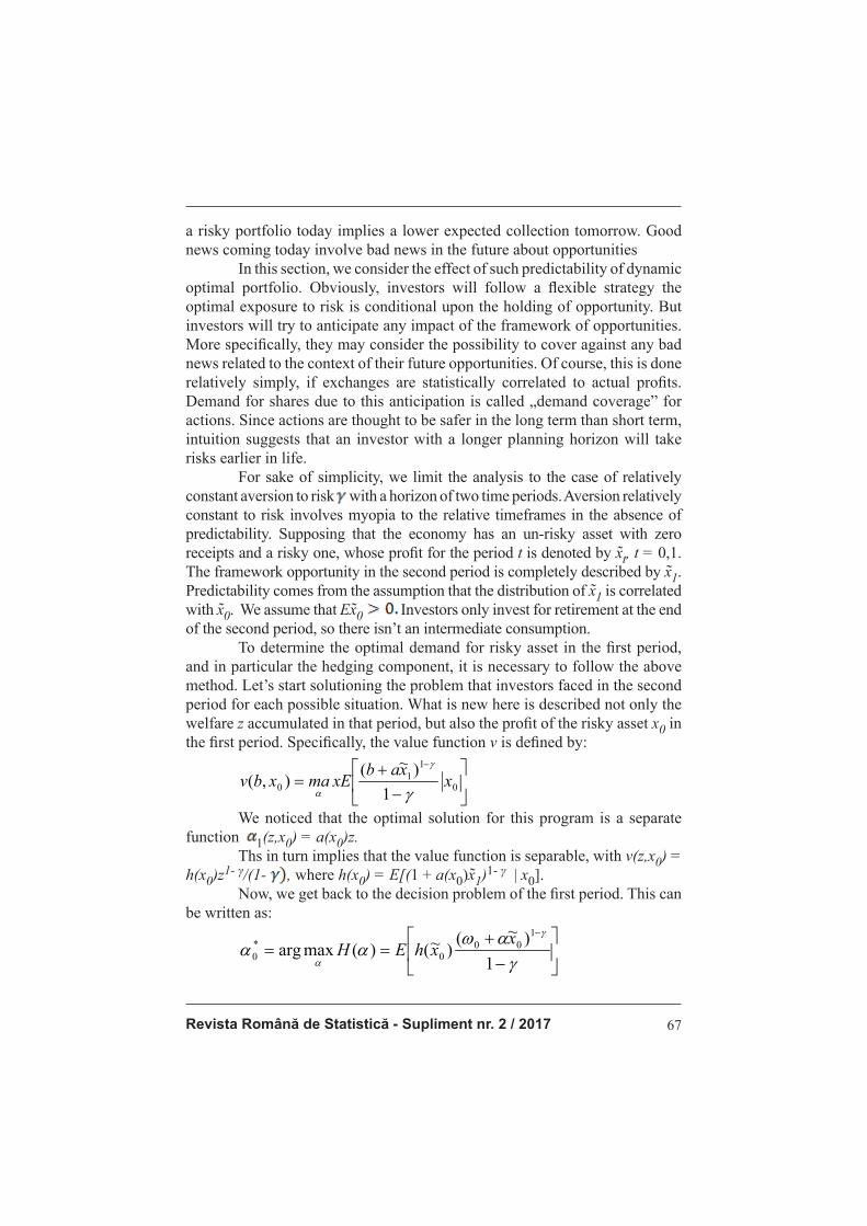
Revista Română de Statistică - Supliment nr. 2 / 2017 67

a risky portfolio today implies a lower expected collection tomorrow. Good news coming today involve bad news in the future about opportunities In this section, we consider the effect of such predictability of dynamic optimal portfolio. Obviously, investors will follow a fl exible strategy the

optimal exposure to risk is conditional upon the holding of opportunity. But

investors will try to anticipate any impact of the framework of opportunities.

More specifi cally, they may consider the possibility to cover against any bad news related to the context of their future opportunities. Of course, this is done relatively simply, if exchanges are statistically correlated to actual profi ts. Demand for shares due to this anticipation is called „demand coverage” for actions. Since actions are thought to be safer in the long term than short term, intuition suggests that an investor with a longer planning horizon will take risks earlier in life. For sake of simplicity, we limit the analysis to the case of relatively constant aversion to risk with a horizon of two time periods. Aversion relatively constant to risk involves myopia to the relative timeframes in the absence of predictability. Supposing that the economy has an un-risky asset with zero receipts and a risky one, whose profi t for the period t is denoted by x̃t, t = 0,1. The framework opportunity in the second period is completely described by x̃1. Predictability comes from the assumption that the distribution of x̃1 is correlated with x̃0. We assume that Ex̃0 Investors only invest for retirement at the end of the second period, so there isn’t an intermediate consumption. To determine the optimal demand for risky asset in the fi rst period, and in particular the hedging component, it is necessary to follow the above method. Let’s start solutioning the problem that investors faced in the second period for each possible situation. What is new here is described not only the welfare z accumulated in that period, but also the profi t of the risky asset x0 in the fi rst period. Specifi cally, the value function v is defi ned by:

�

��

��

�

�

��

�

.

$

$.

$

)H#)�# #

#�+#���#+�

�

�

�

H

H

We noticed that the optimal solution for this program is a separate function 1(z,x0) = a(x0)z. Ths in turn implies that the value function is separable, with v(z,x0) = h(x0)z1- γ/(1- , where h(x0) = E[(1 + a(x0)x̃1)1- γ | x0]. Now, we get back to the decision problem of the fi rst period. This can be written as:

−

+==

−

γαω

ααγ

α 1

)~()~()(maxarg

100

0*0

xxhEH

Romanian Statistical Review - Supplement nr. 2 / 201768

To determine the hedging component for risky asset demand, we compare 0* to demand for risky assets when there is no predictability, for example when x̃1 is independent of x̃0. In this case, we know that myopia is optimal. Thus, in the absence of predictability investors reach the version:

−

+=

−

γαω

αγ

α 1

)~(maxarg

100

0

xEm

When profi ts are somehow predictable, the hedging demand is defi ned as 0*- 0

m. This request for hedging it will be positive if its derivative H

evaluated at 0m

is positive. In other words, the relationship becomes

H’(α0m)=E[x̃ 0h(x̃ 0)(ω0+ α0

m x̃ 0)-ϒ]≥0

Everytime E[x̃0(w0+ 0m x̃0) 1- γ]=0

To evaluate a specifi c type of predictability, we will examine if an increase in x0 will deteriorate x̃1 distribution in the sense of fi rst order stochastic dominance (FSD). A special case is when the stochastic process (x̃0, x̃1) indicates a reversal of means. Supposing that the conditional distribution of x̃1 can be written as x̃1| x̃0= - x0+ , where is assumed as independent of x̃0 and where k it is a positive scalar. Since any change of FSD in x̃1 reduces EU of fi nal welfare, this assumption implies 0 negative. Since v(z,x0) is equal to h(x0)z1- γ/(1- γ), that h’ must be negative when γ <1 and h’ when γ>1.Let’s suppose that the relative risk aversion of γ is greater than unity. Since h’ should be positive in this case, it follows that for all x0, x 0h(x 0) (w0+ 0

m x0) -ϒ≥ x 0h(0) (w0+ 0m x0) -ϒ

For the second situation H’(α0

m) ≥h(0)E[x̃0(w0+ 0m x̃0) 1- γ]=0

Thus, the demand for hedging is positive when the aversion relative to risk is greater than unity. If we have a relative risk aversion less than unity, γ <1, then h’ is negative and the above inequality is reversed. This result is shown in the following sentence. Supposing that a profi t growth from the fi rst period is deteriorating profi t distribution profi t of the second period for the purposes of the fi rst order stochastic dominance. Then, the hedging demand for risky assets is positive (or negative) if risk aversion is relative constant to larger (respectively smaller) than unity. Another way to interpret this result is the following: when relative risk aversion is constant and greater than unity, a longer time horizon should induce to investors a more risk-taking desire. The opposite is true if relative

Revista Română de Statistică - Supliment nr. 2 / 2017 69

risk aversion is lower than unity. Let us note that when investors have a logarithmic utility function (γ =1) myopia is still optimal in the presence of predictability. Choosing an initial risk portfolio is dictated by the collapse of marginal value of wealth at the end of the initial period. This marginal value of wealth depends on the opportunities frame. If predictability reduces the marginal value of welfare in its abundance states, and makes it grow where it is low, then predictability has the same effect as a reduction of risk aversion: it raises the optimum level of risk in the portfolio. As a result, we observe that the central step of the analysis is to determine the effect of the change produced by us that deteriorates FSD in profi ts generated by a risky asset will have the effect it will have on the marginal value of welfare. In the particular case of reversal means, we can see two different effects of the increase in x0. The fi rst effect is the effect of welfare: as expected profi t in the second period becomes smaller, the same happens with welfare, it becomes smaller. This event increases the marginal value of wealth, since v is concave z. The second effect is an effect of caution: investors will invest less in risky assets thus reducing risk exposure. Prudently, it reduces the marginal value of wealth. The global effect of an increase in x0 of the marginal value of wealth is ambiguous. When relative aversion to risk is constant and greater than unity (and this happens if and only if prudence absolute is less than twice aversion absolute towards risk, which explains why this condition implies that the effect of precaution is dominated by wealth effect), the wealth effect always dominates the precaution effect, and demand for hedging is positive. When the relative aversion to risk is less than unity, the wealth effect is dominated by the caution effect. Let’s assume that like in the process of learning Bayes, an increase in profi t in the fi rst period profi t improves distribution in the second period for the purposes of the fi rst order stochastic dominance. Then, the hedging request for risky assets is negative (or positive) if relative constant aversion to risk is larger (or smaller) than unity. Suppose the relative risk aversion is constant and equal to γ =2. Let’s solve the problem of portofolio choice in the secod period conditional on each of the two possible observations made in the fi rst period. I we notice a big profi t in the fi rst period, direct calculation shows that the investor should invest a(2) = 40,22% of his wealth in risky assets in the second period of his life. The value of function v(z,2) is equal to 0,76u(z) in this case. On the other hand, if we notice a low profi t in the fi rst period, optimal investment in the second period would involve a(-1) = -12,67% of wealth invested in the risky asset, and the value function v(z,-1) is equal to 0,97u(z).

Returning to the problem of the fi rst period, the investor resolves the next problem:

Romanian Statistical Review - Supplement nr. 2 / 201770

0,76u(w0+2 + 0,97u(w0- ).

This generates an optimal request for the risky asset from the fi rst period of =7,66% from fi s initial wealth w0. It is easy to verify that the agent who suffers from myopia or acts myopic would invest =12,13%

from his wealth in the risky asset. That’s why, the hedging request -

is negative, thus showing that the learning process tends to induce a prudent

investment behavior in the early stages of learning.

Bibliography

1. Anghelache, C., Anghel, M.G., Manole, A. (2015). Modelare economică, fi nanciar-bancară şi informatică, Editura Artifex, Bucureşti

2. Anghelache, C., Anghel, M.G., Popovici, M. (2015). Multiple Regressions Used in Analysis of Private Consumption and Public Final Consumption Evolution,

International Journal of Academic Research in Accounting, Finance and

Management Sciences, Volume 5, No. 4, October 2015, pp. 69-73

3. Anghelache, C., Soare, D.V., Popovici, M. (2015). Analysis of Gross Domestic Product Evolution under the Infl uence of the Final Consumption, Theoretical and

Applied Economics, Volume XXII, No.4 (605), Winter, pp. 45-52

4. Anghelache, C., Manole, A., Anghel, M.G. (2015). The analysis of the correlation between GDP, private and public consumption through multiple regression,

Romanian Statistical Review - Supplement, No. 8, pp. 34 – 40

5. Anghelache, C., Mitruţ, C., Voineagu, V. (2013). Statistică macroeconomică. Sistemul Conturilor Naţionale, Editura Economică, Bucureşti

6. Anghelache, C., Voineagu, V. (2009). Seriile de timp utilizate ca traiectorii ale proceselor stocastice, Simpozion naţional „Management şi performanţă

economică”, Editura Artifex, pp. 207-214

7. Anghelache, C. (2008). Tratat de statistică teoretică şi economică, Editura

Economică, Bucureşti

8. Anghelache, C., Anghelache, G.V., Bădulescu, M. (2008). Analiza seriilor de timp prin utilizarea metodei spectrale, Revista Română de Statistică Supliment, nr. 3,

pp. 10-26

9. Carroll, C.D. (1997). Buffer-stock saving and the life cycle/permanent income hypothesos, Quarterly Jornal of Economics, 112

10. Deaton, A. (1991). Saving and liquidity constraints, Econometrica, 59

11. Ghysels, E., Osborn, D. (2001). The Econometric Analysis of Seasonal Time Series, Cambridge University Press

12. Hribar, P., McInnis, J. (2012). Investor Sentiment and Analysts’ Earnings Forecast Errors, Management Science 58, no. 2, pg. 293-307

13. Kalaman, O., Zhalinska, O. (2012). Venture capital as a major source of investment in innovation, Journal of Applied Management and Investments,

Volume (Year): 1 (2012), Issue (Month): 1 (), pp. 92-98

14. Ravi, B., Kiku, D., Shaliastovich, I., Yaron, A. (2014). Volatility, the Macroeconomy, and Asset Prices, Journal of Finance 69, no. 6, pg. 2471-2511

Revista Română de Statistică - Supliment nr. 2 / 2017 71

Model de analiză a corelaţiei dintre produsul intern brut şi componentele consumului fi nal

Prof. univ. dr. Constantin ANGHELACHE

Academia de Studii Economice București, Universitatea „ARTIFEX” București

Drd. Andreea Ioana MARINESCU

Academia de Studii Economice din București

Drd. Doina AVRAM

Academia de Studii Economice din București

Drd. Doina BUREA

Academia de Studii Economice din București

Drd. Gyorgy BODO

Academia de Studii Economice din București

Abstract

În acest articol, autorii analizează evoluția Produsul Intern Brut, considerat ca variabilă dependentă, sub infl uența componentelor consumului fi nal. Consumul fi nal al gospodăriilor populației, precum și consumul fi nal

al administrației publice, reprezintă utilizări ale Produsului Intern Brut.

Consumul fi nal poate fi considerat ca un indicator major al dinamicii

economiei României, prin urmare analiza infl uenței sale asupra creșterii

economice va produce rezultate corespunzătoare.

Cuvinte cheie: Consum, PIB, public, privat, regresie

Clasifi care JEL: E01, E21

Introducere

Consumul fi nal este unul dintre factorii care infl uențează formarea

Produsului Intern Brut, conform metodei cheltuielilor. Alături de metodele

de analiză a dinamicii și structurii, studiul indicatorilor clasici ai seriilor

de timp, metoda regresiei oferă rezultate cu un nivel de complexitate mai

ridicat asupra infl uenței componentelor consumului fi nal asupra indicatorului

macroeconomic de rezultate – PIB.

Literature review

Alesina, Campante și Tabellini (2008) dezvoltă pe tema caracterului

ciclic al politicilor fi scale. Andrei et.al. (2008) se preocupă de utilizarea

aplicației Eviews în studii econometrice. Anghelache și Anghel (2016) este o

lucrare de referință în statistica economică, autorii abordează și problematica

indicatorilor macroeconomici. Aplicarea modelului de regresie în analize

Romanian Statistical Review - Supplement nr. 2 / 201772

economice a fost evidențiată în lucrările publicate de Anghelache, Manole

și Anghel (2015), Anghelache și Popovici (2015), Anghelache, Anghel et.al. (2015), Anghelache, Marinescu și Manole (2009). Battaglini, și Coate (2008) descriu aspecte teoretice legate de consumul public, fi scalitate și datorie. Corbae, Durlauf și Hansen (2006), Guijarati (2005), Wooldrige (2006) au publicat cărți de referință în domeniul econometriei. Herwartz (1997) se

preocupă de modelele de previziune a consumului. Lucas (2003) analizează

prioritățile macroeconomice. Mitroi și Oproiu (2013) evaluează legătura

dintre creditele de consum și veniturile gospodăriilor în România. Mountford

și Uhlig (2009) descriu efectele șocurilor politicii fi scale.

Metodologia cercetării și date. Rezultate și analiză

Modelul de regresie unifactorial poate fi utilizat şi pentru stabilirea infl uenţei pe care o are valoarea consumului asupra evoluţiei Produsului Intern Brut al României. În acest sens am utilizat serii de date cu o frecvență anuală acoperind perioada 1990-2016, iar pentru a asigura comparabilitatea datelor le-am defl atat, luând ca bază anul 1990, prin împărţirea la Indicele Preţului de Consum din anul respectiv a valorilor nominale ale PIB-ului și ale consumului privat. Analiza corelaţiei dintre PIB și consumul privat presupune, într-o primă etapă, analiza individuală a fi ecărei mărimi considerate. În cazul Produsul Intern Brut analiza a fost efectuată anterior, nefi ind necesară o revenire asupra aspectelor constatate cu acest prilej. În ceea ce priveşte evoluţia consumului privat în România, seria de date a fost procesată cu ajutorul programului informatic Eviews, ceea ce a permis obţinerea unor informaţii semnifi cative referitoare la variaţia acestui indicator macroeconomic în perioada 1990-2016.

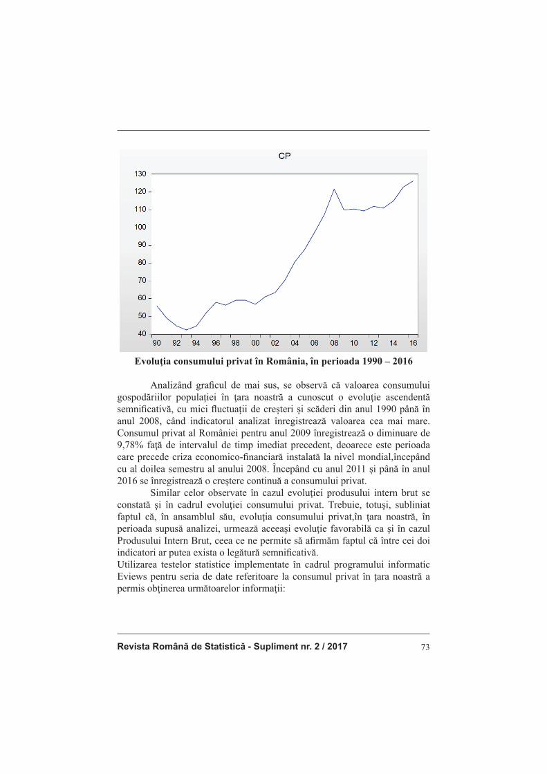
Revista Română de Statistică - Supliment nr. 2 / 2017 73

Evoluţia consumului privat în România, în perioada 1990 – 2016

Analizând grafi cul de mai sus, se observă că valoarea consumului gospodăriilor populației în ţara noastră a cunoscut o evoluţie ascendentă semnifi cativă, cu mici fl uctuații de creșteri și scăderi din anul 1990 până în anul 2008, când indicatorul analizat înregistrează valoarea cea mai mare. Consumul privat al României pentru anul 2009 înregistrează o diminuare de 9,78% faţă de intervalul de timp imediat precedent, deoarece este perioada care precede criza economico-fi nanciară instalată la nivel mondial,începând cu al doilea semestru al anului 2008. Începând cu anul 2011 și până în anul 2016 se înregistrează o creștere continuă a consumului privat. Similar celor observate în cazul evoluţiei produsului intern brut se constată şi în cadrul evoluţiei consumului privat. Trebuie, totuşi, subliniat faptul că, în ansamblul său, evoluţia consumului privat,în ţara noastră, în perioada supusă analizei, urmează aceeaşi evoluţie favorabilă ca şi în cazul Produsului Intern Brut, ceea ce ne permite să afi rmăm faptul că între cei doi indicatori ar putea exista o legătură semnifi cativă.Utilizarea testelor statistice implementate în cadrul programului informatic Eviews pentru seria de date referitoare la consumul privat în ţara noastră a permis obţinerea următoarelor informaţii:

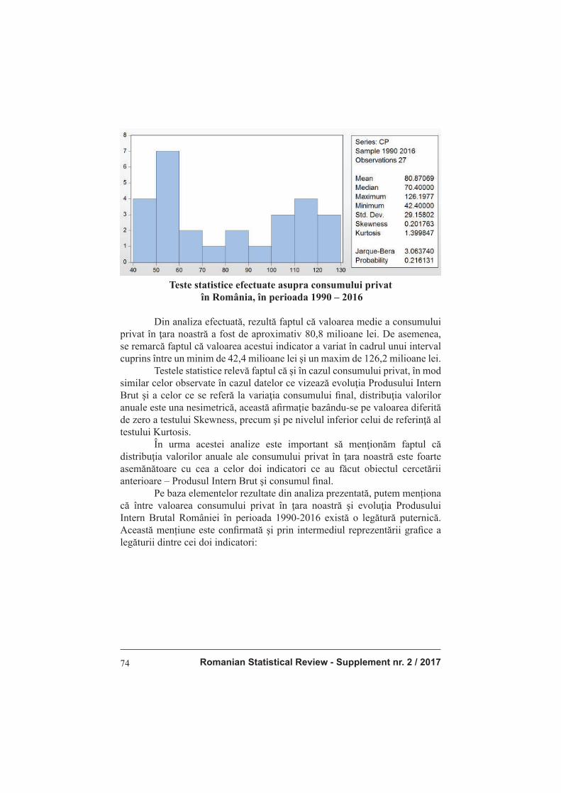
Romanian Statistical Review - Supplement nr. 2 / 201774

Teste statistice efectuate asupra consumului privat

în România, în perioada 1990 – 2016

Din analiza efectuată, rezultă faptul că valoarea medie a consumului privat în ţara noastră a fost de aproximativ 80,8 milioane lei. De asemenea, se remarcă faptul că valoarea acestui indicator a variat în cadrul unui interval cuprins între un minim de 42,4 milioane lei şi un maxim de 126,2 milioane lei.

Testele statistice relevă faptul că şi în cazul consumului privat, în mod

similar celor observate în cazul datelor ce vizează evoluţia Produsului Intern Brut şi a celor ce se referă la variaţia consumului fi nal, distribuţia valorilor anuale este una nesimetrică, această afi rmaţie bazându-se pe valoarea diferită de zero a testului Skewness, precum şi pe nivelul inferior celui de referinţă al testului Kurtosis. În urma acestei analize este important să menţionăm faptul că distribuţia valorilor anuale ale consumului privat în ţara noastră este foarte asemănătoare cu cea a celor doi indicatori ce au făcut obiectul cercetării anterioare – Produsul Intern Brut şi consumul fi nal. Pe baza elementelor rezultate din analiza prezentată, putem menționa că între valoarea consumului privat în ţara noastră şi evoluţia Produsului Intern Brutal României în perioada 1990-2016 există o legătură puternică. Această mențiune este confi rmată şi prin intermediul reprezentării grafi ce a legăturii dintre cei doi indicatori:

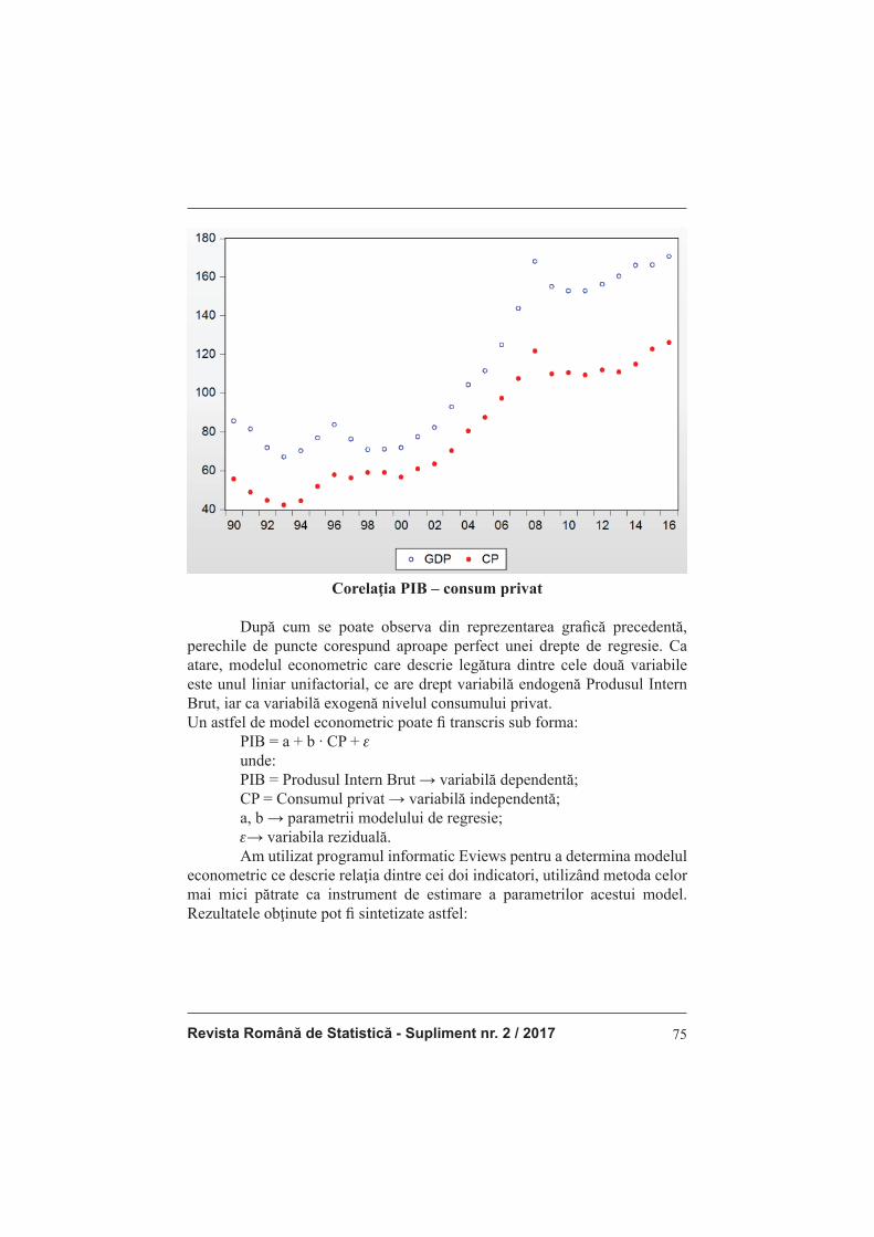
Revista Română de Statistică - Supliment nr. 2 / 2017 75

Corelaţia PIB – consum privat

După cum se poate observa din reprezentarea grafi că precedentă, perechile de puncte corespund aproape perfect unei drepte de regresie. Ca atare, modelul econometric care descrie legătura dintre cele două variabile este unul liniar unifactorial, ce are drept variabilă endogenă Produsul Intern Brut, iar ca variabilă exogenă nivelul consumului privat.Un astfel de model econometric poate fi transcris sub forma: PIB = a + b ∙ CP + e

unde:

PIB = Produsul Intern Brut → variabilă dependentă;

CP = Consumul privat → variabilă independentă;

a, b → parametrii modelului de regresie;

e→ variabila reziduală.

Am utilizat programul informatic Eviews pentru a determina modelul

econometric ce descrie relaţia dintre cei doi indicatori, utilizând metoda celor

mai mici pătrate ca instrument de estimare a parametrilor acestui model.

Rezultatele obţinute pot fi sintetizate astfel:

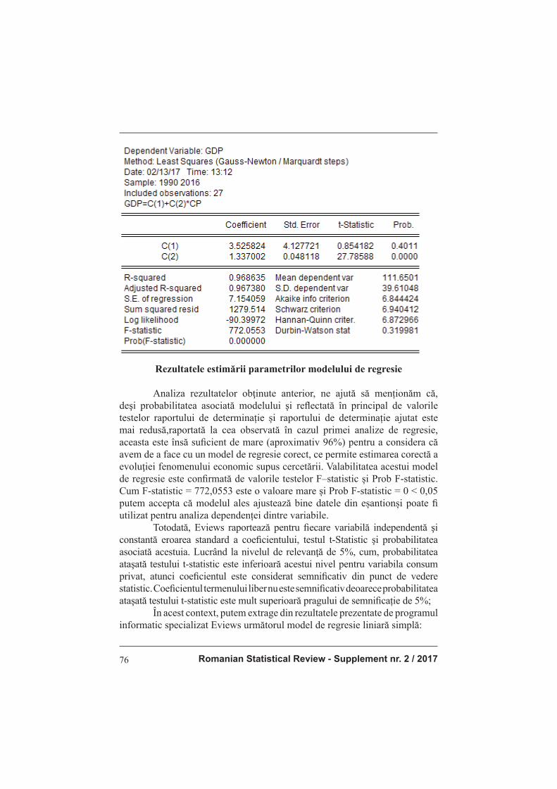
Romanian Statistical Review - Supplement nr. 2 / 201776

Rezultatele estimării parametrilor modelului de regresie

Analiza rezultatelor obţinute anterior, ne ajută să menționăm că, deşi probabilitatea asociată modelului şi refl ectată în principal de valorile testelor raportului de determinație și raportului de determinație ajutat este mai redusă,raportată la cea observată în cazul primei analize de regresie, aceasta este însă sufi cient de mare (aproximativ 96%) pentru a considera că avem de a face cu un model de regresie corect, ce permite estimarea corectă a evoluţiei fenomenului economic supus cercetării. Valabilitatea acestui model de regresie este confi rmată de valorile testelor F–statistic și Prob F-statistic. Cum F-statistic = 772,0553 este o valoare mare și Prob F-statistic = 0 < 0,05 putem accepta că modelul ales ajustează bine datele din eșantionși poate fi utilizat pentru analiza dependenței dintre variabile. Totodată, Eviews raportează pentru fi ecare variabilă independentă şi constantă eroarea standard a coefi cientului, testul t-Statistic şi probabilitatea asociată acestuia. Lucrând la nivelul de relevanţă de 5%, cum, probabilitatea ataşată testului t-statistic este inferioară acestui nivel pentru variabila consum privat, atunci coefi cientul este considerat semnifi cativ din punct de vedere statistic. Coefi cientul termenului liber nu este semnifi cativ deoarece probabilitatea ataşată testului t-statistic este mult superioară pragului de semnifi cație de 5%; În acest context, putem extrage din rezultatele prezentate de programul informatic specializat Eviews următorul model de regresie liniară simplă:

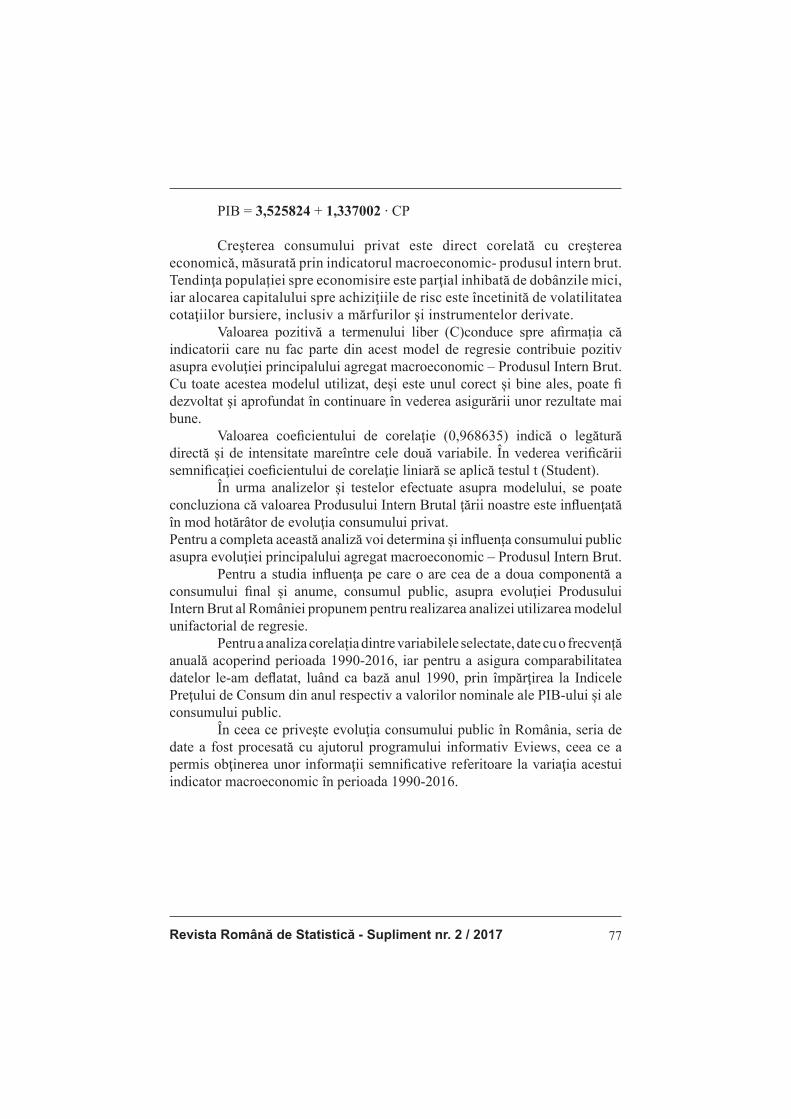
Revista Română de Statistică - Supliment nr. 2 / 2017 77

PIB = 3,525824 + 1,337002 ∙ CP

Creşterea consumului privat este direct corelată cu creşterea

economică, măsurată prin indicatorul macroeconomic- produsul intern brut.

Tendinţa populației spre economisire este parţial inhibată de dobânzile mici, iar alocarea capitalului spre achiziţiile de risc este încetinită de volatilitatea cotaţiilor bursiere, inclusiv a mărfurilor şi instrumentelor derivate. Valoarea pozitivă a termenului liber (C)conduce spre afi rmația că indicatorii care nu fac parte din acest model de regresie contribuie pozitiv asupra evoluţiei principalului agregat macroeconomic – Produsul Intern Brut. Cu toate acestea modelul utilizat, deși este unul corect și bine ales, poate fi dezvoltat şi aprofundat în continuare în vederea asigurării unor rezultate mai bune. Valoarea coefi cientului de corelaţie (0,968635) indică o legătură directă și de intensitate mareîntre cele două variabile. În vederea verifi cării semnifi caţiei coefi cientului de corelaţie liniară se aplică testul t (Student). În urma analizelor și testelor efectuate asupra modelului, se poate concluziona că valoarea Produsului Intern Brutal ţării noastre este infl uenţată în mod hotărâtor de evoluţia consumului privat. Pentru a completa această analiză voi determina și infl uența consumului public asupra evoluţiei principalului agregat macroeconomic – Produsul Intern Brut. Pentru a studia infl uenţa pe care o are cea de a doua componentă a consumului fi nal și anume, consumul public, asupra evoluţiei Produsului Intern Brut al României propunem pentru realizarea analizei utilizarea modelul unifactorial de regresie. Pentru a analiza corelația dintre variabilele selectate, date cu o frecvență anuală acoperind perioada 1990-2016, iar pentru a asigura comparabilitatea datelor le-am defl atat, luând ca bază anul 1990, prin împărţirea la Indicele Preţului de Consum din anul respectiv a valorilor nominale ale PIB-ului și ale consumului public. În ceea ce priveşte evoluţia consumului public în România, seria de date a fost procesată cu ajutorul programului informativ Eviews, ceea ce a permis obţinerea unor informaţii semnifi cative referitoare la variaţia acestui indicator macroeconomic în perioada 1990-2016.

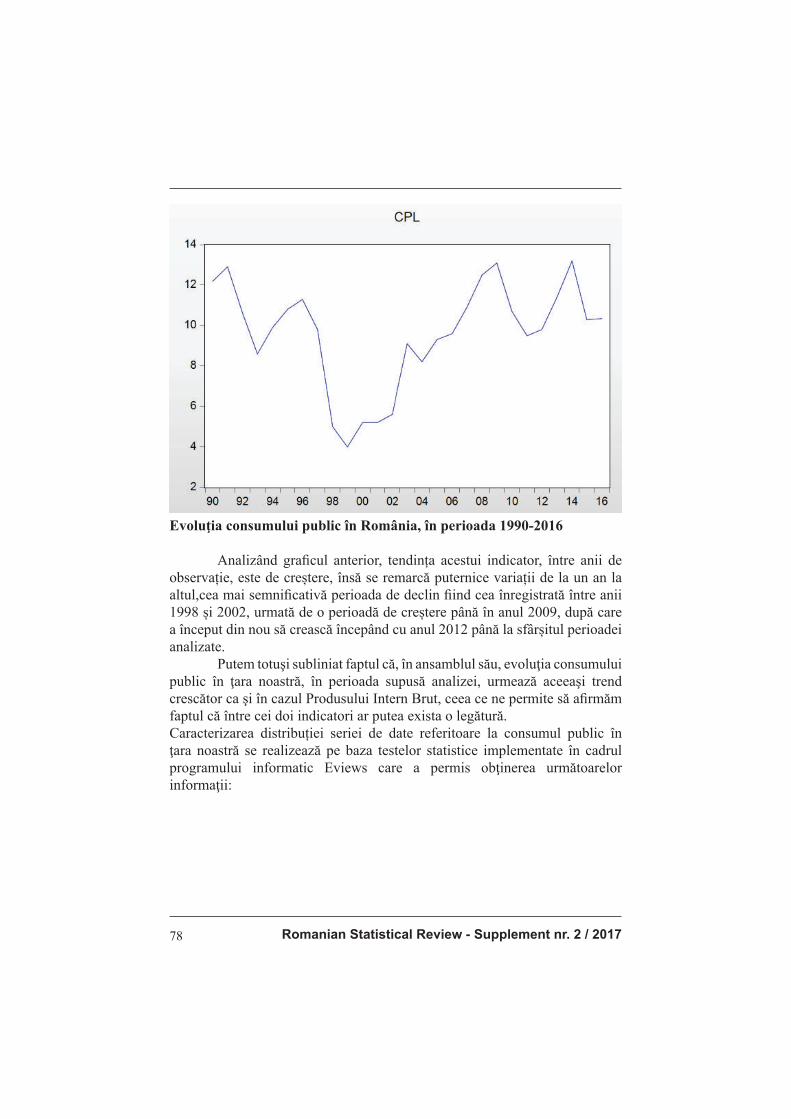
Romanian Statistical Review - Supplement nr. 2 / 201778

Evoluţia consumului public în România, în perioada 1990-2016

Analizând grafi cul anterior, tendința acestui indicator, între anii de observație, este de creștere, însă se remarcă puternice variații de la un an la altul,cea mai semnifi cativă perioada de declin fi ind cea înregistrată între anii 1998 și 2002, urmată de o perioadă de creștere până în anul 2009, după care a început din nou să crească începând cu anul 2012 până la sfârșitul perioadei analizate. Putem totuşi subliniat faptul că, în ansamblul său, evoluţia consumului

public în ţara noastră, în perioada supusă analizei, urmează aceeaşi trend

crescător ca şi în cazul Produsului Intern Brut, ceea ce ne permite să afi rmăm

faptul că între cei doi indicatori ar putea exista o legătură.

Caracterizarea distribuției seriei de date referitoare la consumul public în

ţara noastră se realizează pe baza testelor statistice implementate în cadrul

programului informatic Eviews care a permis obţinerea următoarelor

informaţii:

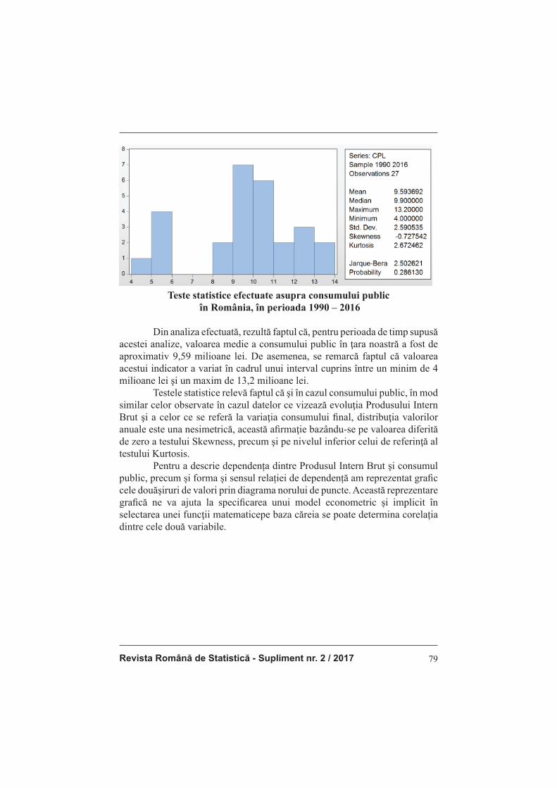
Revista Română de Statistică - Supliment nr. 2 / 2017 79

Teste statistice efectuate asupra consumului public

în România, în perioada 1990 – 2016

Din analiza efectuată, rezultă faptul că, pentru perioada de timp supusă acestei analize, valoarea medie a consumului public în ţara noastră a fost de aproximativ 9,59 milioane lei. De asemenea, se remarcă faptul că valoarea acestui indicator a variat în cadrul unui interval cuprins între un minim de 4

milioane lei şi un maxim de 13,2 milioane lei.

Testele statistice relevă faptul că şi în cazul consumului public, în mod

similar celor observate în cazul datelor ce vizează evoluţia Produsului Intern Brut şi a celor ce se referă la variaţia consumului fi nal, distribuţia valorilor anuale este una nesimetrică, această afi rmaţie bazându-se pe valoarea diferită de zero a testului Skewness, precum şi pe nivelul inferior celui de referinţă al testului Kurtosis. Pentru a descrie dependența dintre Produsul Intern Brut şi consumul public, precum și forma și sensul relației de dependență am reprezentat grafi c cele douășiruri de valori prin diagrama norului de puncte. Această reprezentare grafi că ne va ajuta la specifi carea unui model econometric și implicit în selectarea unei funcţii matematicepe baza căreia se poate determina corelația dintre cele două variabile.

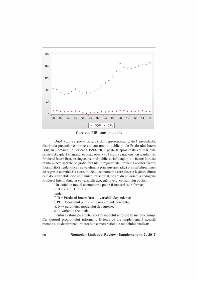
Romanian Statistical Review - Supplement nr. 2 / 201780

Corelaţia PIB- consum public

După cum se poate observa din reprezentarea grafi că precedentă,

distribuția punctelor empirice ale consumului public şi ale Produsului Intern Brut, în România, în perioada 1990- 2016 poate fi aproximata cel mai bine printr-o dreapta. Din grafi c, se poate observa că asupra caracteristicii rezultative,

Produsul Intern Brut, pe lângăconsumul public, au infl uențat și alti factori întrucât

există puncte așezate pe grafi c fără nici o regularitate, infl uența acestor factori

întâmplători neidentifi cați se va elimina prin ajustare, adică prin stabilirea liniei

de regresie teoretică.Ca atare, modelul econometric care descrie legătura dintre

cele două variabile este unul liniar unifactorial, ce are drept variabilă endogenă

Produsul Intern Brut, iar ca variabilă exogenă nivelul consumului public.

Un astfel de model econometric poate fi transcris sub forma:

PIB = a + b ∙ CPL + e

unde:

PIB = Produsul Intern Brut → variabilă dependentă;

CPL = Consumul public → variabilă independentă;

a, b → parametrii modelului de regresie;

e → variabila reziduală.

Pentru a estima parametrii acestui modelul se folosește metoda cmmp.

Cu ajutorul programului informatic Eviews ce are implementată această

metodă s-au determinat următoarele caracteristici ale modelului analizat:

Revista Română de Statistică - Supliment nr. 2 / 2017 81

Rezultatele estimării parametrilor modelului de regresie

Analizând rezultatele obţinute anterior se pot face următoarele precizări referitoare la legătura dintre cei doi indicatori, după cum urmează: - R-squared, coefi cientul de determinaţie, R2 = 0.26 arată că 26 % din variația produsului intern brut este explicată de nivelul consumului public; se poate afi rma că, modifi carea consumului public nu constituie un factor hotărâtor în variația produsului intern brut; - Pentru fi ecare variabilă independentă şi constantă Eviews raportează eroarea standard a coefi cientului, testul t-Statistic şi probabilitatea asociată acestuia. Lucrând la nivelul de relevanţă de 5%, cum, probabilitatea ataşată testului t-statistic este inferioară acestui nivel pentru variabila consum prublic, atunci coefi cientul este considerat semnifi cativ din punct de vedere statistic. Coefi cientul termenului liber nu este semnifi cativ deoarece probabilitatea ataşată testului t-statistic este superioară pragului de semnifi cație de 5%; - Valabilitatea acestui model de regresie este confi rmată de valorile testelor F–statistic și Prob F-statistic. Cum F-statistic calculat este superior nivelului tabelat și Prob F-statistic = 0,0058 < 0,05 putem accepta că modelul ales ajustează bine datele din eșantion și poate fi utilizat pentru analiza dependenței dintre variabile. În acest context, putem extrage din rezultatele prezentate de programul informatic specializat Eviews următorul model de regresie liniară simplă:

Romanian Statistical Review - Supplement nr. 2 / 201782

PIB = 35,89882 + 7,895944 ∙ CPL

Valoarea ridicată a termenului liber refl ectă faptul că infl uenţa factorilor, care nu au fost luaţi în considerare la momentul construcţiei acestui model de regresie contribuie semnifi cativ asupra evoluţiei principalului agregat macroeconomic – Produsul Intern Brut. Cu toate aceastea modelul utilizat, deși este unul corect și bine ales, poate fi dezvoltat şi aprofundat în vederea asigurării unor rezultate mai bune pentru activitatea de previzionare. Valoarea coefi cientului de corelaţie indică o legătură directă și moderată între cele două variabile. În vederea verifi cării semnifi caţiei coefi cientului de corelaţie liniară se aplică testul t (Student).

Concluzii

Modifi carea cu un milion lei a consumului privat determină creșterea Produsului Intern Brut cu 1,33 milioane lei, dovadă a legăturii directe între cele două variabile studiate. La creşterea cu un milion lei a consumului public, Produsul Intern Brut va crește cu 7,89 milioane lei, ceea ce subliniază existența legăturii directe între cele două variabile studiate. În urma analizelor și testelor efectuate, se poate concluziona că valoarea Produsului Intern Brutal ţării noastre este infl uenţată moderat de evoluţia consumului public și, într-o manieră mai semnifi cativă, de cea a consumului privat. Pentru ambele cazuri de corelaţie studiate, am obţinut valori semnifi cative pentru termenul constant, ceea ce face dovada infl uenţei factorilor neluaţi în considerare la estimarea modelelor de regresie, dar care contribuie semnifi cativ la evoluţia PIB.

Bibliografi e

1. Alesina, A., Campante, F., Tabellini, G. (2008). Why is Fiscal Policy Often Procyclical, Journal of the European Economic Association, 6, 5, 1006–1036

2. Andrei, T., Stancu, S., Iacob, A., Erika, T. (2008). Introducere în econometrie

utilizând Eviews, Editura Economică, Bucureşti 3. Anghelache, C., Anghel, M.G. (2016). Bazele statisticii economice. Concepte

teoretice şi studii de caz, Editura Economică, Bucureşti 4. Anghelache, C., Manole, A. (2016). Utilizarea modelului de regresie în analiza

corelaţiei dintre situaţia monetară şi balanţa de plăţi / The use of regression model

in analysing the correlation between the monetary situation and the balance of

payments, Romanian Statistical Review, Supplement, no.7, pp. 24-29 / 30-42 5. Anghelache, C., Manole, A., Anghel, M.G. (2015). Analysis of fi nal consumption

and gross investment infl uence on GDP – multiple linear regression model, Theoretical and Applied Economics, No. 3/2015 (604), Autumn, pp. 137-142

6. Anghelache, C., Popovici, M. (2015). Analysis Theoretical Model of the

Consumption from the Gross Domestic Product, Romanian Statistical Review

Revista Română de Statistică - Supliment nr. 2 / 2017 83

Supplement, No. 11, pp. 57-62 7. Anghelache, C., Anghel, M.G., Prodan, L., Sacală, C., Popovici, M. (2015).

Elements concerning the Use of Multiple Regression Models, Romanian Statistical Review Supplement, Issue 4, pp. 27-29

8. Anghelache, C., Marinescu, R.T., Manole M. (2009). Estimarea şi utilizarea funcţiei de regresie prin nucleu, Supliment al Revistei Române de Statistică, nr. 12/2009, pp. 103-106

9. Battaglini, M., Coate, S. (2008). A Dynamic Theory of Public Spending, Taxation and Debt, American Economic Review, 98 (1), pp. 201–236

10. Corbae, D., Durlauf, S., Hansen, B. (2006). Econometric Theory and Practice, Frontiers and Analysis and Applied Research, Cambridge University Press

11. Guijarati, D. (2005). Basic Econometrics, The McGraw – Hill Companies 12. Herwartz, H. (1997). Performance and Periodic Error Correction Models in

Forecasting Consumption Data, International Journal of Forecasting, 13, 421 – 431

13. Lucas, R.E. Jr. (2003). Macroeconomic Priorities, American Economic Review, 93(1), pp. 1-14

14. Mitroi, A., Oproiu, A. (2013). Analysis of the correlation between the evolution of the consumer loans and the evolution of household income in Romania, Theoretical and Applied Economics, No. 12 (589), pp. 67-82

15. Mountford, A., Uhlig, H. (2009). What are the effects of fi scal policy

shocks?, Journal of Applied Econometrics, 24 (6), pp. 960-992 16. Wooldrige, J. (2006). Introductory econometrics. A modern approach – 2 edition,

MIT Press

Romanian Statistical Review - Supplement nr. 2 / 201784

MODEL ANALYSIS OF THE CORRELATION BETWEEN GDP AND FINAL CONSUMPTION

COMPONENTS

Prof. Constantin ANGHELACHE PhD.

Bucharest University of Economic Studies, „ARTIFEX” University of Bucharest

Andreea Ioana MARINESCU PhD. Student

Bucharest University of Economic Studies

Doina AVRAM PhD. Student

Bucharest University of Economic Studies

Doina BUREA PhD. Student

Bucharest University of Economic Studies

Gyorgy BODO PhD. Student

Bucharest University of Economic Studies

Abstract

In this paper, authors analyze the evolution of the Gross Domestic

Product, considered as dependent variable, under the infl uence of the

components of fi nal consumption. The fi nal consumption of households, and

the fi nal consumption of public administration, are uses of the Gross Domestic

Product. The fi nal consumption can be considered as a major indicator of

the Romanian economy dynamics, so the analysis of its infl uence, thus the

analysis on its infl uence on economic growth will provide valuable results.

Key words: Consumption, GDP, public, private, regression

JEL Classifi cation: E01, E21

Introduction

The fi nal consumption is one of the factors that infl uence the formation

of the Gross Domestic Product, according to the expenses method. Together with

methods that analyse the dynamics and the structure, the study of classical indicators

of time series, the regression offers more complex results on the infl uences of fi nal

consumption components on the macroeconomic results measure – the GDP.

Literature review

Alesina, Campante and Tabellini (2008) develop on the topic of

cyclical character of fi scal policies. Andrei et.al. (2008) are preoccupied with

the use of Eviews in econometric studies. Anghelache and Anghel (2016)

is a reference work in economic statistics, the authors approach the issues

regarding macroeconomic indicators. The application of the regression model

Revista Română de Statistică - Supliment nr. 2 / 2017 85

in economic analyses was emphasized in the papers published by Anghelache, Manole and Anghel (2015), Anghelache and Popovici (2015), Anghelache, Anghel et.al. (2015), Anghelache, Marinescu and Manole (2009). Battaglini and Coate (2008) describe theoretical aspects regarding public consumption, taxation and debt. Corbae, Durlauf and Hansen (2006), Guijarati (2005), Wooldrige (2006) have published reference books for econometrics. Herwartz (1997) is preoccupied with consumption forecast models. Lucas (2003) analyses the macroeconomic priorities. Mitroi and Oproiu (2013) evaluate the link between consumption credits and households income in Romania. Mountford and Uhlig (2009) describe the effects of taxation policy shocks.

Research methodology and data. Results and analysis

Unifactorial regression model can be used to establish the infl uence of private consumption is set on the evolution of Romania’s Gross Domestic Product. Thus, we used data on a yearly basis covering the period 1990-2016, and to ensure that data we defl ated, taking as the base year 1990 by dividing by the Consumer Price Index for that year denominations of GDP and private consumption. In this regard, we considered a number of data on the evolution of the two aforementioned macroeconomic indicators during 1990-2016. We shall measure the correlation between GDP and private consumption, this involves a fi rst stage, the individual analysis of each size. As regards private consumption trends in Romania, the data set was processed using Eviews, which enabled obtaining meaningful information on the movement in the macroeconomic indicators during 1990-2016.

The evolution of private consumption in Romania during 1990 - 2016

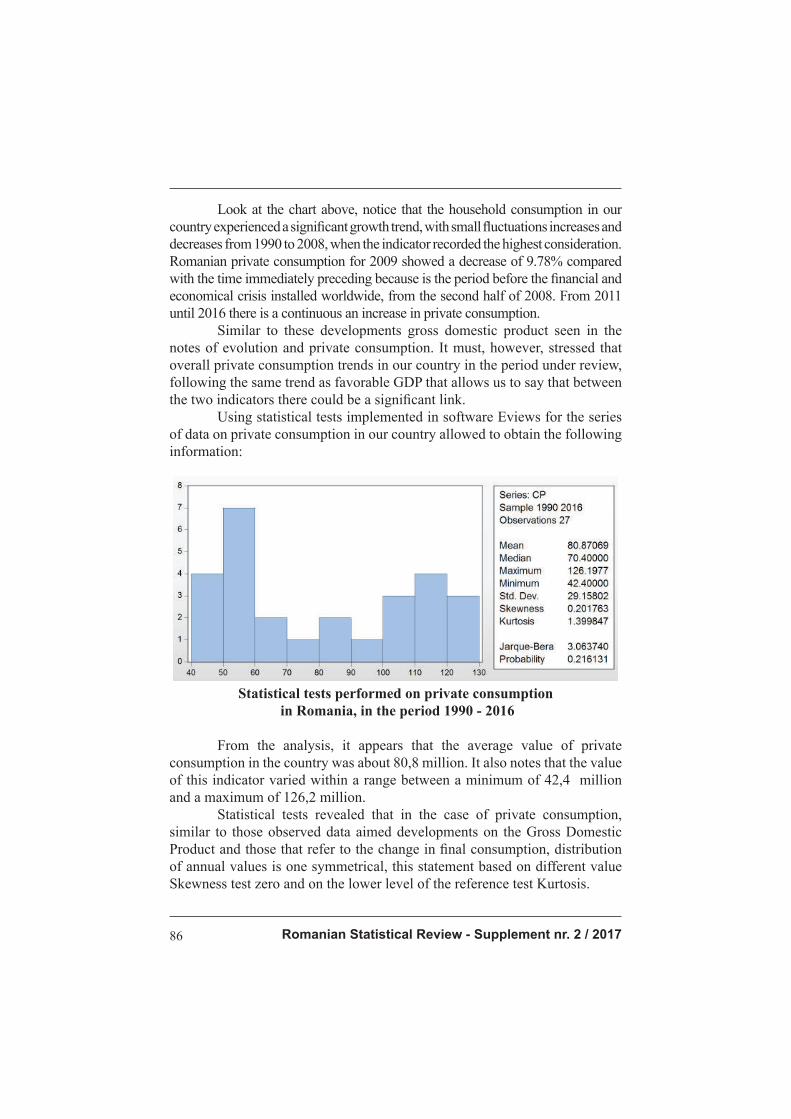
Romanian Statistical Review - Supplement nr. 2 / 201786

Look at the chart above, notice that the household consumption in our country experienced a signifi cant growth trend, with small fl uctuations increases and

decreases from 1990 to 2008, when the indicator recorded the highest consideration.

Romanian private consumption for 2009 showed a decrease of 9.78% compared with the time immediately preceding because is the period before the fi nancial and

economical crisis installed worldwide, from the second half of 2008. From 2011

until 2016 there is a continuous an increase in private consumption.

Similar to these developments gross domestic product seen in the

notes of evolution and private consumption. It must, however, stressed that

overall private consumption trends in our country in the period under review,

following the same trend as favorable GDP that allows us to say that between

the two indicators there could be a signifi cant link.

Using statistical tests implemented in software Eviews for the series

of data on private consumption in our country allowed to obtain the following

information:

Statistical tests performed on private consumption

in Romania, in the period 1990 - 2016

From the analysis, it appears that the average value of private

consumption in the country was about 80,8 million. It also notes that the value

of this indicator varied within a range between a minimum of 42,4 million

and a maximum of 126,2 million.

Statistical tests revealed that in the case of private consumption,

similar to those observed data aimed developments on the Gross Domestic

Product and those that refer to the change in fi nal consumption, distribution

of annual values is one symmetrical, this statement based on different value

Skewness test zero and on the lower level of the reference test Kurtosis.

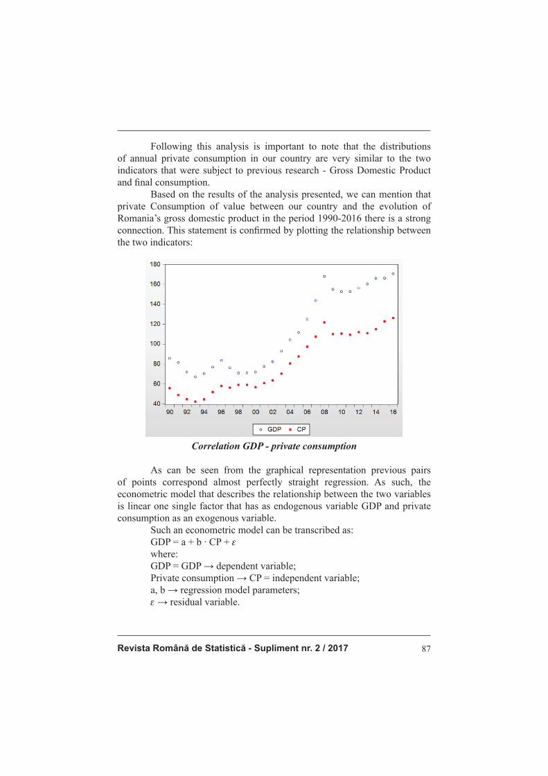
Revista Română de Statistică - Supliment nr. 2 / 2017 87

Following this analysis is important to note that the distributions of annual private consumption in our country are very similar to the two indicators that were subject to previous research - Gross Domestic Product and fi nal consumption.

Based on the results of the analysis presented, we can mention that

private Consumption of value between our country and the evolution of

Romania’s gross domestic product in the period 1990-2016 there is a strong

connection. This statement is confi rmed by plotting the relationship between

the two indicators:

Correlation GDP - private consumption

As can be seen from the graphical representation previous pairs

of points correspond almost perfectly straight regression. As such, the

econometric model that describes the relationship between the two variables

is linear one single factor that has as endogenous variable GDP and private

consumption as an exogenous variable.

Such an econometric model can be transcribed as:

GDP = a + b ∙ CP + e

where:

GDP = GDP → dependent variable;

Private consumption → CP = independent variable;

a, b → regression model parameters;

e → residual variable.

Romanian Statistical Review - Supplement nr. 2 / 201788

We used the software Eviews to determine the econometric model that describes the relationship between the two indicators using least squares as a tool for estimating the parameters of this model. The results can be summarized as follows:

The results of the regression model parameter estimates

Analysis of the results obtained previously, helps us to note that although the probability associated with the model and mainly refl ected the values of the tests report determinaţieşi report determination helped is reduced relative to that observed in the fi rst regression analysis, it is however big enough (about 96%) to believe that we are dealing with a regression

model correctly, that allows accurate estimation of the evolution of economic

phenomena under investigation. The validity of this model is confi rmed by

the regression test values F-statistic and F-statistic Prob. How F-statistic =

772,0553 is a great value and Prob F-statistic = 0 <0.05 can accept the model

chosen sample and well adjusted data can be used to analyze the dependence

between variables.

However, Eviews reported for each independent variable and constant

coeffi cient standard error, t-test and the Statistical probability associated with

it. Working at 5% level of relevance, as the probability attached statistical

t-test is below this level for private consumption variable, the coeffi cient is

considered statistically signifi cant. Free term coeffi cient is not signifi cant

because the probability attached statistical t-test is far superior materiality of

5%;

Revista Română de Statistică - Supliment nr. 2 / 2017 89

In this context, we can draw from the results presented by specialized software Eviews following simple linear regression model:

GDP = 3,525824 + 1,337002 ∙ CP

Private consumption growth is directly correlated with economic

growth, measured by gross domestic product indicator macroeconomic-.

Population trend towards saving is partially inhibited by low-interest rates

and risk capital allocation for acquisitions is slowed by the volatility of stock

prices, including freight and derivatives.

The positive free term (C) leads to the affi rmation that the indicators that are not part of this regression model contributes positively to the evolution of macroeconomic aggregate principal - GDP. Although this model used, although it is a fair and well chosen, can be developed and expanded further to ensure better results. The correlation coeffi cient (0,968635) indicates a direct and intensity link between the two variables. In order to verify the signifi cance of the correlation coeffi cient is applied t test (Student). The analyses and tests on the model, it can be concluded that the value of our country’s gross domestic product is signifi cantly infl uenced by

developments in private consumption.

To complete this analysis will determine and infl uence public

consumption on the evolution of macroeconomic aggregate principal - GDP.

To study the infl uence that has the second component of fi nal

consumption ie public consumption, on the evolution of Romania’s Gross

Domestic Product we intend to achieve single factor analysis using regression

model.

To analyze the correlation between selected variables, given with an

annual frequency covering the period 1990-2016, and to ensure comparability

of data we defl ated, taking as the base year 1990 by dividing by the Consumer

Price Index for that year denominations of GDP community and public

consumption.

Regarding public consumption trends in Romania, the data set was

processed using Eviews, which enabled obtaining meaningful information on

the movement in the macroeconomic indicators during 1990-2016.

Romanian Statistical Review - Supplement nr. 2 / 201790

The evolution of public consumption in Romania during 1990-2016

Looking at the chart above, the trend of this indicator, the years of observation, it decreases the but stands strong variations from year to year, the most signifi cant period of decline as that recorded between 1998 and 2002,

followed by a period of growth until 2009, then began to rise again from 2012

until the end of the period.

We nevertheless stressed that, as a whole, developments in public

consumption in our country, in the period under review, following the same

upward trend as for GDP, which allows us to say that between the two

indicators there may be a link.

Characterization distribution data series on public consumption in our

country is based on statistical tests implemented in the software Eviews which

allowed to obtain the following information:

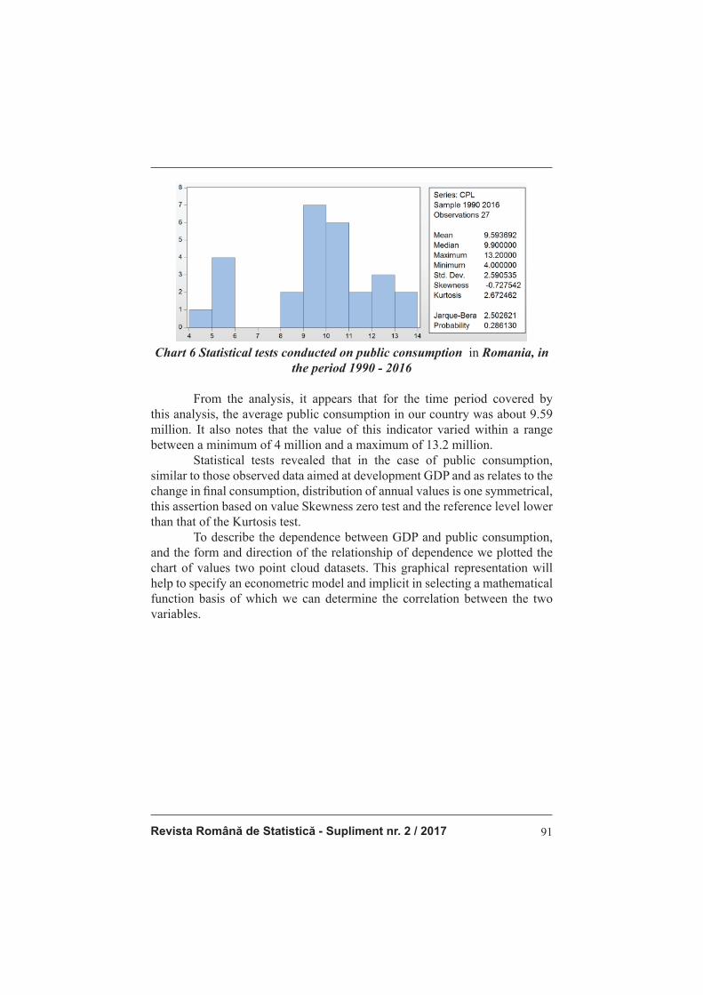
Revista Română de Statistică - Supliment nr. 2 / 2017 91

Chart 6 Statistical tests conducted on public consumption in Romania, in

the period 1990 - 2016

From the analysis, it appears that for the time period covered by this analysis, the average public consumption in our country was about 9.59 million. It also notes that the value of this indicator varied within a range between a minimum of 4 million and a maximum of 13.2 million. Statistical tests revealed that in the case of public consumption, similar to those observed data aimed at development GDP and as relates to the change in fi nal consumption, distribution of annual values is one symmetrical,

this assertion based on value Skewness zero test and the reference level lower

than that of the Kurtosis test.

To describe the dependence between GDP and public consumption,

and the form and direction of the relationship of dependence we plotted the

chart of values two point cloud datasets. This graphical representation will

help to specify an econometric model and implicit in selecting a mathematical

function basis of which we can determine the correlation between the two

variables.

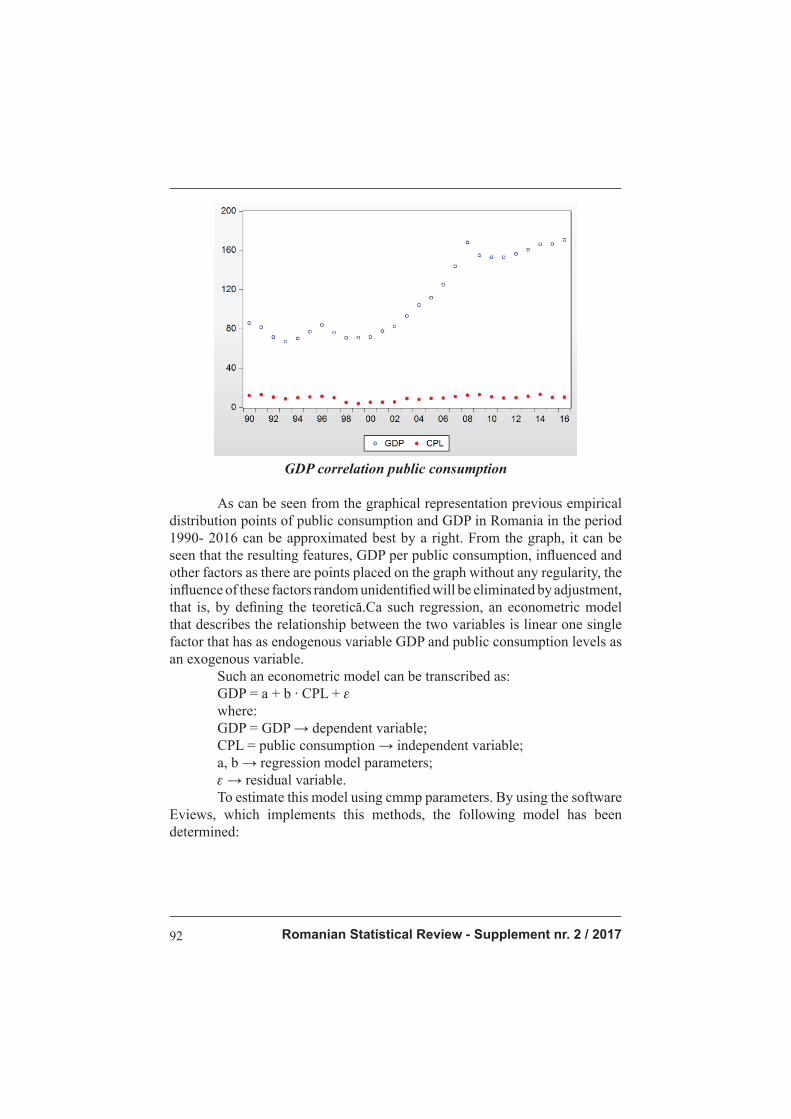
Romanian Statistical Review - Supplement nr. 2 / 201792

GDP correlation public consumption

As can be seen from the graphical representation previous empirical distribution points of public consumption and GDP in Romania in the period 1990- 2016 can be approximated best by a right. From the graph, it can be seen that the resulting features, GDP per public consumption, infl uenced and other factors as there are points placed on the graph without any regularity, the infl uence of these factors random unidentifi ed will be eliminated by adjustment, that is, by defi ning the teoretică.Ca such regression, an econometric model

that describes the relationship between the two variables is linear one single

factor that has as endogenous variable GDP and public consumption levels as

an exogenous variable.

Such an econometric model can be transcribed as:

GDP = a + b ∙ CPL + e

where:

GDP = GDP → dependent variable;

CPL = public consumption → independent variable;

a, b → regression model parameters;

e → residual variable.

To estimate this model using cmmp parameters. By using the software

Eviews, which implements this methods, the following model has been

determined:

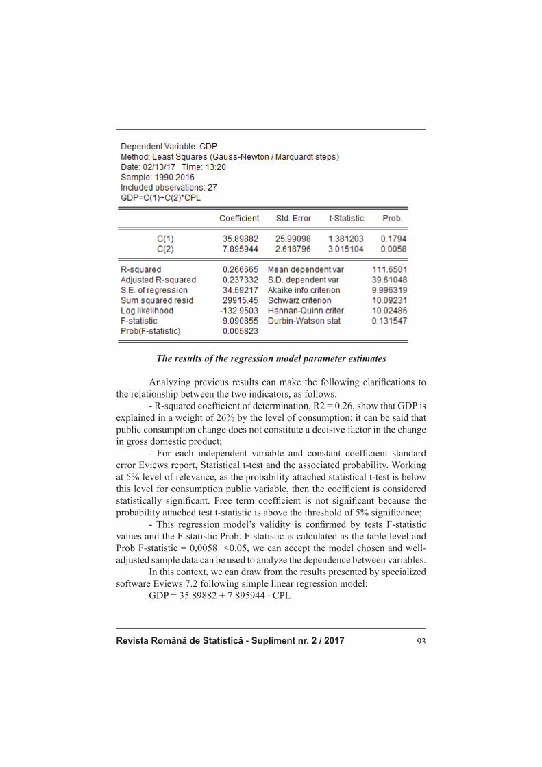
Revista Română de Statistică - Supliment nr. 2 / 2017 93

The results of the regression model parameter estimates

Analyzing previous results can make the following clarifi cations to

the relationship between the two indicators, as follows:

- R-squared coeffi cient of determination, R2 = 0.26, show that GDP is

explained in a weight of 26% by the level of consumption; it can be said that public consumption change does not constitute a decisive factor in the change in gross domestic product; - For each independent variable and constant coeffi cient standard

error Eviews report, Statistical t-test and the associated probability. Working

at 5% level of relevance, as the probability attached statistical t-test is below this level for consumption public variable, then the coeffi cient is considered

statistically signifi cant. Free term coeffi cient is not signifi cant because the

probability attached test t-statistic is above the threshold of 5% signifi cance;

- This regression model’s validity is confi rmed by tests F-statistic

values and the F-statistic Prob. F-statistic is calculated as the table level and

Prob F-statistic = 0,0058 <0.05, we can accept the model chosen and well-

adjusted sample data can be used to analyze the dependence between variables.

In this context, we can draw from the results presented by specialized

software Eviews 7.2 following simple linear regression model:

GDP = 35.89882 + 7.895944 ∙ CPL

Romanian Statistical Review - Supplement nr. 2 / 201794

The high value of the constant term that refl ects the infl uence of factors which were not taken into account when building the regression model contributes signifi cantly to the evolution of macroeconomic aggregate principal - GDP. Although this model used, although it is a fair and well chosen, can be developed and deepened in order to ensure better outcomes for business forecasting. The correlation coeffi cient indicates a moderate direct connection between the two variables. In order to verify the signifi cance of the correlation coeffi cient is applied t test (Student).

Conclusions

The modifi cation by one million lei in private consumption, leads to the GDP growth by 1.13 million, evidence of the existence of a direct link between the two variables studied. The increase of one million lei public consumption, GDP will grow by 7.89 million, which outlines the existence of a direct link between the two variables studied. From the analyses and tests performed, it can be concluded that the value of the gross domestic product of our country is infl uenced by public and, more signifi cant, by the private consumption trends. For both correlation case studied, we have achieved a high value of the constant term, that provides evidence on the infl uence of factors not taken into consideration when estimating the regression models, but they contribute signifi cantly to the evolution of GDP.

References

1. Alesina, A., Campante, F., Tabellini, G. (2008). Why is Fiscal Policy Often Procyclical, Journal of the European Economic Association, 6, 5, 1006–1036

2. Andrei, T., Stancu, S., Iacob, A., Erika, T. (2008). Introducere în econometrie

utilizând Eviews, Editura Economică, Bucureşti

3. Anghelache, C., Anghel, M.G. (2016). Bazele statisticii economice. Concepte

teoretice şi studii de caz, Editura Economică, Bucureşti

4. Anghelache, C., Manole, A. (2016). Utilizarea modelului de regresie în analiza corelaţiei dintre situaţia monetară şi balanţa de plăţi / The use of regression model

in analysing the correlation between the monetary situation and the balance of

payments, Romanian Statistical Review, Supplement, no.7, pp. 24-29 / 30-42

5. Anghelache, C., Manole, A., Anghel, M.G. (2015). Analysis of fi nal consumption

and gross investment infl uence on GDP – multiple linear regression model,

Theoretical and Applied Economics, No. 3/2015 (604), Autumn, pp. 137-142

6. Anghelache, C., Popovici, M. (2015). Analysis Theoretical Model of the

Consumption from the Gross Domestic Product, Romanian Statistical Review

Supplement, No. 11, pp. 57-62

7. Anghelache, C., Anghel, M.G., Prodan, L., Sacală, C., Popovici, M. (2015).

Revista Română de Statistică - Supliment nr. 2 / 2017 95

Elements concerning the Use of Multiple Regression Models, Romanian Statistical Review Supplement, Issue 4, pp. 27-29

8. Anghelache, C., Marinescu, R.T., Manole M. (2009). Estimarea şi utilizarea funcţiei de regresie prin nucleu, Supliment al Revistei Române de Statistică, nr. 12/2009, pp. 103-106

9. Battaglini, M., Coate, S. (2008). A Dynamic Theory of Public Spending, Taxation and Debt, American Economic Review, 98 (1), pp. 201–236

10. Corbae, D., Durlauf, S., Hansen, B. (2006). Econometric Theory and Practice, Frontiers and Analysis and Applied Research, Cambridge University Press

11. Guijarati, D. (2005). Basic Econometrics, The McGraw – Hill Companies 12. Herwartz, H. (1997). Performance and Periodic Error Correction Models in

Forecasting Consumption Data, International Journal of Forecasting, 13, 421 – 431

13. Lucas, R.E. Jr. (2003). Macroeconomic Priorities, American Economic Review, 93(1), pp. 1-14

14. Mitroi, A., Oproiu, A. (2013). Analysis of the correlation between the evolution of the consumer loans and the evolution of household income in Romania, Theoretical and Applied Economics, No. 12 (589), pp. 67-82

15. Mountford, A., Uhlig, H. (2009). What are the effects of fi scal policy

shocks?, Journal of Applied Econometrics, 24 (6), pp. 960-992 16. Wooldrige, J. (2006). Introductory econometrics. A modern approach – 2 edition,

MIT Press

Romanian Statistical Review - Supplement nr. 2 / 201796

Model de analiză a corelaţiei dintre consumul fi nal şi componentele acestuia

Prof. univ. dr. Alexandru MANOLE

Universitatea „ARTIFEX” din București

Lector univ. dr. Mariana BUNEA

Universitatea „ARTIFEX” din București

Lector univ. dr. Ana CARP

Universitatea „ARTIFEX” din București

Asist. Univ. Dr. Diana-Valentina SOARE

Universitatea „ARTIFEX” din București

Drd. Maria MIREA

Academia de Studii Economice din București

Abstract

În acest articol, autorii abordează analiza consumului fi nal. Metodologia urmăreşte componentele consumului fi nal, respectiv consumul corespunzător administraţiei publice, precum şi consumul referitor la gospodăriile populaţiei. Instrumentele econometrice oferă rezultate relevante

pentru un set de date care acoperă un interval de timp mai extins, din 1990 în

2016. Rezultatele estimării modelului sunt discutate de autori.

Cuvinte cheie: consum, fi nal, estimare, model, impact Clasifi care JEL: E01, E21

Introducere

Analiza de față își propune ca prin intermediul unui model unifactorial de regresie să stabilească infl uenţa consumului privat al României din perioada 1990-2016 asupra consumului fi nal din aceeaşi perioadă.

Analiza corelaţiei dintre cei doi indicatori presupune, într-o primă

etapă, cercetarea individuală a fi ecărei mărimi considerate. Reprezentările

grafi ce permit analiza vizuală a corelaţiei dintre indicatori şi oferă o bază

pentru continuarea studiului şi estimarea unui model de regresie.

Literature review

Andersen et.al. (2003) se preocupă de modelarea şi previzionarea

volatilităţii. Bardsen, Nymagen şi Jansen (2005), Anghelache şi Anghel (2016)

au publicat lucrări de referinţă în aplicarea instrumentelor econometrice în

analiza economică. Anghelache, Manole şi Anghel (2015), Anghelache,

Anghel şi Popovici (2015) studiază infl uenţa consumului privat asupra

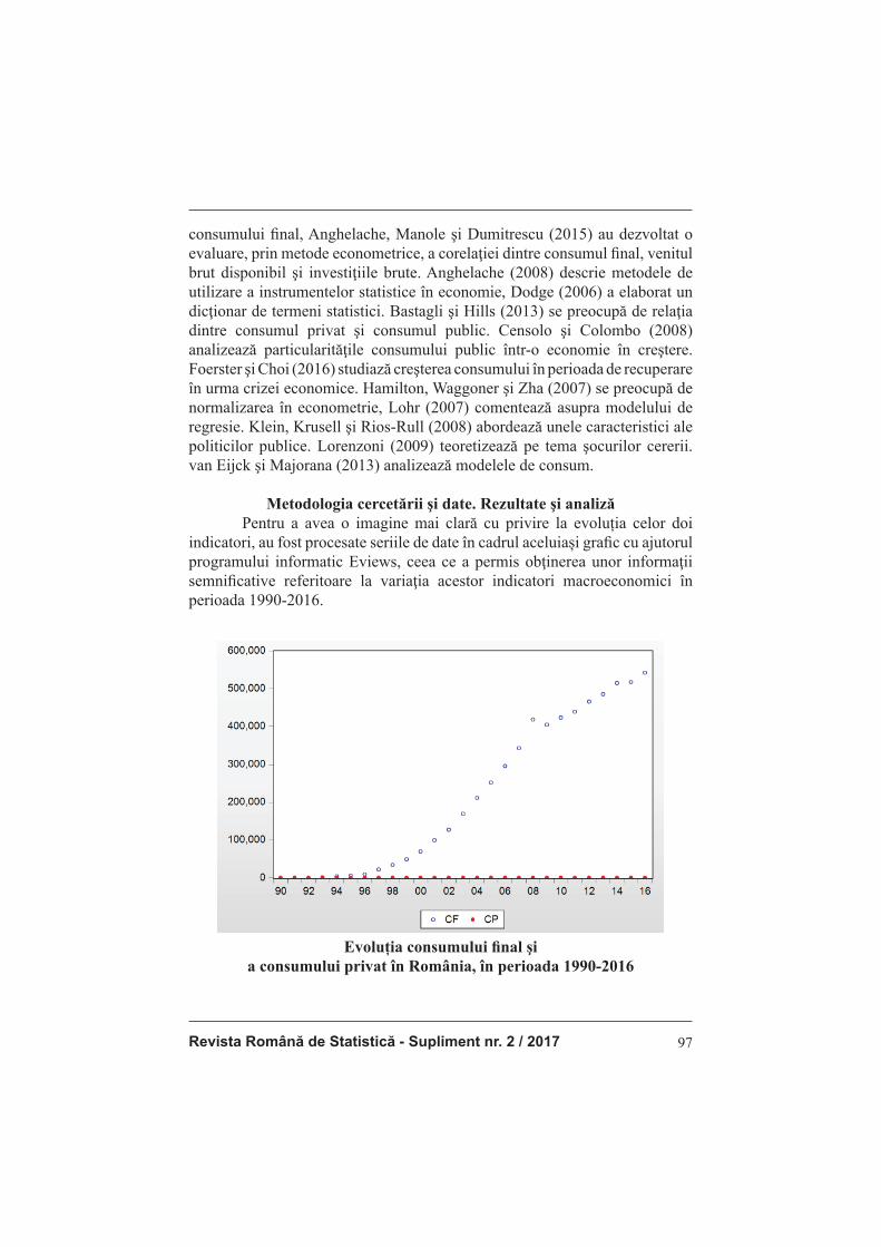
Revista Română de Statistică - Supliment nr. 2 / 2017 97

consumului fi nal, Anghelache, Manole şi Dumitrescu (2015) au dezvoltat o

evaluare, prin metode econometrice, a corelaţiei dintre consumul fi nal, venitul

brut disponibil şi investiţiile brute. Anghelache (2008) descrie metodele de

utilizare a instrumentelor statistice în economie, Dodge (2006) a elaborat un

dicţionar de termeni statistici. Bastagli şi Hills (2013) se preocupă de relaţia

dintre consumul privat şi consumul public. Censolo şi Colombo (2008)

analizează particularităţile consumului public într-o economie în creştere.

Foerster şi Choi (2016) studiază creşterea consumului în perioada de recuperare

în urma crizei economice. Hamilton, Waggoner şi Zha (2007) se preocupă de

normalizarea în econometrie, Lohr (2007) comentează asupra modelului de

regresie. Klein, Krusell şi Rios-Rull (2008) abordează unele caracteristici ale

politicilor publice. Lorenzoni (2009) teoretizează pe tema şocurilor cererii.

van Eijck şi Majorana (2013) analizează modelele de consum.

Metodologia cercetării şi date. Rezultate şi analiză

Pentru a avea o imagine mai clară cu privire la evoluția celor doi

indicatori, au fost procesate seriile de date în cadrul aceluiași grafi c cu ajutorul

programului informatic Eviews, ceea ce a permis obţinerea unor informaţii

semnifi cative referitoare la variaţia acestor indicatori macroeconomici în

perioada 1990-2016.

Evoluția consumului fi nal şi

a consumului privat în România, în perioada 1990-2016

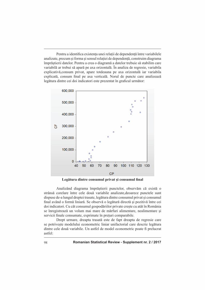
Romanian Statistical Review - Supplement nr. 2 / 201798

Pentru a identifi ca existența unei relații de dependență între variabilele analizate, precum și forma și sensul relației de dependență, construim diagrama împrăștierii datelor. Pentru a crea o diagramă a datelor trebuie să stabilim care variabilă ar trebui să apară pe axa orizontală. În analiza de regresie, variabila explicativă,consum privat, apare totdeauna pe axa orizontală iar variabila explicată, consum fi nal pe axa verticală. Norul de puncte care analizează legătura dintre cei doi indicatori este prezentat în grafi cul următor:

Legătura dintre consumul privat și consumul fi nal

Analizând diagrama împrăștierii punctelor, observăm că există o strânsă corelare între cele două variabile analizate,deoarece punctele sunt dispuse de-a lungul dreptei trasate, legătura dintre consumul privat și consumul fi nal având o formă liniară. Se observă o legătură directă și pozitivă între cei doi indicatori. Cu cât consumul gospodăriilor private crește cu atât în România se înregistrează un volum mai mare de mărfuri alimentare, nealimentare și servicii fi nale consumate, exprimate în prețuri comparabile. Drept urmare, dreapta trasată este de fapt dreapta de regresie care se potrivește modelului econometric liniar unifactorial care descrie legătura dintre cele două variabile. Un astfel de model econometric poate fi prelucrat astfel:

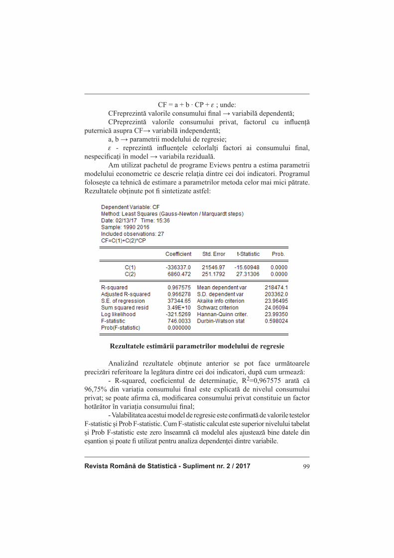
Revista Română de Statistică - Supliment nr. 2 / 2017 99

CF = a + b ∙ CP + e ; unde:

CFreprezintă valorile consumului fi nal → variabilă dependentă;

CPreprezintă valorile consumului privat, factorul cu infl uență

puternică asupra CF→ variabilă independentă;

a, b → parametrii modelului de regresie;

e - reprezintă infl uențele celorlalți factori ai consumului fi nal,

nespecifi cați în model → variabila reziduală.

Am utilizat pachetul de programe Eviews pentru a estima parametrii

modelului econometric ce descrie relaţia dintre cei doi indicatori. Programul

folosește ca tehnică de estimare a parametrilor metoda celor mai mici pătrate.

Rezultatele obţinute pot fi sintetizate astfel:

Rezultatele estimării parametrilor modelului de regresie

Analizând rezultatele obţinute anterior se pot face următoarele

precizări referitoare la legătura dintre cei doi indicatori, după cum urmează:

- R-squared, coefi cientul de determinaţie, R2=0,967575 arată că

96,75% din variația consumului fi nal este explicată de nivelul consumului

privat; se poate afi rma că, modifi carea consumului privat constituie un factor

hotărâtor în variația consumului fi nal;

- Valabilitatea acestui model de regresie este confi rmată de valorile testelor

F-statistic și Prob F-statistic. Cum F-statistic calculat este superior nivelului tabelat

și Prob F-statistic este zero înseamnă că modelul ales ajustează bine datele din

eșantion și poate fi utilizat pentru analiza dependenței dintre variabile.

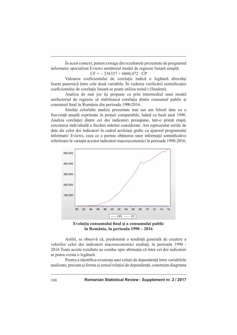
Romanian Statistical Review - Supplement nr. 2 / 2017100

În acest context, putem extrage din rezultatele prezentate de programul informatic specializat Eviews următorul model de regresie liniară simplă:

CF = - 336337 + 6860,472 ∙ CP

Valoarea coefi cientului de corelaţie indică o legătură directăși foarte puternică între cele două variabile. În vederea verifi cării semnifi caţiei coefi cientului de corelaţie liniară se poate utiliza testul t (Student). Analiza de mai jos își propune ca prin intermediul unui model unifactorial de regresie să stabilească corelația dintre consumul public și consumul fi nal în România din perioada 1990-2016. Similar celorlalte analize prezentate mai sus am folosit date cu o frecvență anuală exprimate în prețuri comparabile, luând ca bază anul 1990. Analiza corelaţiei dintre cei doi indicatori presupune, într-o primă etapă, cercetarea individuală a fi ecărei mărimi considerate. Am reprezentat seriile de date ale celor doi indicatori în cadrul aceluiași grafi c cu ajutorul programului informativ Eviews, ceea ce a permis obţinerea unor informaţii semnifi cative referitoare la variaţia acestor indicatori macroeconomici în perioada 1990-2016.

Evoluția consumului fi nal şi a consumului publicîn România, în perioada 1990 – 2016

Astfel, se observă că, predomină o tendință generală de creștere a valorilor celor doi indicatori macroeconomici studiați, în perioada 1990 - 2016 Toate aceste rezultate ne conduc spre afi rmația că între cei doi indicatori ar putea exista o legătură. Pentru a identifi ca existența unei relații de dependență între variabilele analizate, precum și forma și sensul relației de dependență, construim diagrama

Revista Română de Statistică - Supliment nr. 2 / 2017 101

împrăștierii datelor. Pentru a crea o diagramă a datelor trebuie să stabilim care

variabilă ar trebui să apară pe axa orizontală. Prin urmare, variabila consum

public se consideră a fi cauza sau variabila independentă (explicativă sau

factorială), variantele ei notându-se cu xi, iar variabila consum fi nal este

considerată efect sau variabilă dependentă (explicată sau rezultativă),

variantele ei notându-se cu yi.

Diagrama de dispersie prezintă perechile (xi, yi) sub forma unui nor de

puncte în planul (x, y). Reprezentarea grafi că ajută la aproximarea modelului

de regresie.

Legătura dintre consumul public și consumul fi nal

După cum se poate observa din reprezentarea grafi că precedentă,

distribuția punctelor empirice ale consumului public şi ale consumului fi nal în

România, în perioada 1990-2016, sugerează o legătură liniară și slabă deoarece

norul de puncte este difuz. Merită menţionat faptul că nivelul consumului

fi nal realizat depinde, în afară de consumul public, de mulţi alţi factori, cum

ar fi consumul privat, venitul disponibil etc.,întrucât există puncte așezate pe

grafi c fără nici o regularitate; infl uența acestor factori întâmplători neidentifi cați

se va elimina prin ajustare, adică prin stabilirea liniei de regresie teoretică.

Analizând grafi cul de mai sus, constatăm că mulţimea perechilor de

valori (xi,yi ) refl ectă o legătură statistică directă (pe măsură ce xieste mai mare

Romanian Statistical Review - Supplement nr. 2 / 2017102

şi yi tinde să fi e mai mare). Ca atare, între cele două variabile, se constată, deci,

o legătură liniară, directă, ce are drept variabilă endogenă consumul fi nal, iar

ca variabilă exogenă nivelul consumului public.

Un astfel de model econometric poate fi transcris sub forma:

CF = a + b ∙ CPL + e

unde:

CF reprezintă valorile consumului fi nal → variabilă dependentă;

CPL reprezintă valorile defl atate ale consumului public → variabilă

independentă;

a, b → parametrii modelului de regresie;

e - reprezintă infl uențele celorlalți factori ai consumului fi nal,

nespecifi cați în model→ variabila reziduală.

Utilizarea pachetului de programe Eviews pentru estimarea

parametrilor modelului econometric descris mai sus, a condus la obţinerea

următoarelor rezultate:

Rezultatele estimării parametrilor modelului de regresie

Analizând rezultatele obţinute anterior se desprind următoarele

concluzii:

- R-squared, coefi cientul de determinaţie, 13,3646 arată că aproximativ

13,36% din variația consumului fi nal poate fi explicată de nivelul consumului

public; se poate afi rma că, modifi carea consumului public nu constituie un

factor hotărâtor în variația consumului fi nal;

Revista Română de Statistică - Supliment nr. 2 / 2017 103

- Pentru fi ecare variabilă independentă şi constantă Eviews raportează eroarea standard a coefi cientului, testul t-Statistic şi probabilitatea asociată acestuia. Lucrând la nivelul de relevanţă de 5%, cum, probabilitatea ataşată testului t-statistic este inferioară acestui nivel pentru variabila consum public, atunci coefi cientul este considerat semnifi cativ din punct de vedere statistic. Coefi cientul termenului liber nu este semnifi cativ deoarece probabilitatea ataşată testului t-statistic este superioară pragului de semnifi cație de 5%; În acest context, putem extrage din rezultatele prezentate de programul informatic specializat Eviews următorul model de regresie liniară simplă:

CF = -56849,69 + 28698,42∙ CPL Semnul pozitiv al coefi cientul de regresie confi rmă cele prezentate mai sus, adică existența unei legături directe între cele două variabile studiate.

Concluzii

Evoluția consumului fi nal este infl uențată în mod hotărâtor de variația consumului privat, în timp ce este infl uenţată slab de evoluţia consumului public. Valoarea ridicată a termenului liber refl ectă faptul că infl uenţa factorilor, care nu au fost luaţi în considerare la momentul construcţiei celor două modele de regresie contribuie semnifi cativ asupra evoluţiei consumului fi nal. Cu toate acestea modelele utilizate, deși sunt corecte și bine alese, pot fi dezvoltat şi aprofundat în vederea asigurării unor rezultate mai bune pentru activitatea de previzionare.

Bibliografi e

1. Andersen, T., Bollerslev, T., Diebold, F., Labys, P. (2003). Modeling and

Forecasting Realized Volatility, Econometrica, Volume 71, Issue 2, pp. 579–625 2. Anghelache, C., Anghel, M.G. (2016). Econometrie generală. Concepte, teorie și

studii de caz, Editura Artifex, Bucureşti 3. Anghelache, C., Manole, A., Anghel, M.G. (2015). Unifactorial Econometric

Model - Connection between the Final Consumption and the Private Consumption, Asian Academic Research Journal Of Social Science & Humanities, Volume 2, Issue 6, November 2015, pp. 212-219

4. Anghelache, C., Anghel, M.G., Popovici, M. (2015). Multiple Regressions Used

in Analysis of Private Consumption and Public Final Consumption Evolution, International Journal of Academic Research in Accounting, Finance and Management Sciences, Volume 5, No. 4, October 2015, pp. 69-73

5. Anghelache, C., Manole, A., Dumitrescu, D. (2015). The Correlation between Final

Consumption, Gross Available Income and Gross Investment: An Econometric

Analysis, International Journal of Academic Research in Accounting, Finance and Management Sciences, Vol. 5, Nr. 4, 2015, pp. 84-88

6. Anghelache, C. (2008). Tratat de statistică teoretică şi economică, Editura Economică, Bucureşti

Romanian Statistical Review - Supplement nr. 2 / 2017104

7. Bardsen, G., Nymagen, R., Jansen, E. (2005). The Econometrics of Macroeconomic

Modelling, Oxford University Press 8. Bastagli, F., Hills, J. (2013). What Gives? Household Consumption Patterns

and the‚ Big Trade Off’ with Public Consumption, Centre for Analysis of Social Exclusion, LSE in series CASE Papers with number case170

9. Censolo, R., Colombo, C. (2008). Public consumption composition in

a growingeconomy, Journal of Macroeconomics. Volume (Year): 30 (2008), Issue (Month): 4(December), 1479-1495

10. Dodge, Y. (editor) (2006). The Oxford dictionary of statistical terms, Oxford University Press

11. Foerster, A.T., Choi, J. (2016). Consumption Growth Regimes and the Post-

Financial Crisis Recovery, Economic Review, Volume (Year): (2016), Issue (Month): Q II (), pp. 25-48

12. Hamilton, J., Waggoner, D., Zha, T. (2007). Normalization in econometrics, Econometrics Reviews, nr. 26, pp. 221-252

13. Klein, P., Krusell, P., Rios-Rull, V. (2008). Time-Consistent Public Policy, Review of Economic Studies, 75, pp. 789–808

14. Lohr, S.L. (2007). Comment: Struggles with Survey Weighting and Regression

Modeling, Statistical Science, Vol. 22, No. 2, pp.175–178 15. Lorenzoni, G. (2009). A Theory of Demand Shocks, American Economic Review

99, no. 5, pp. 2050-2084 16. van Eijck, K., Majorana, M. (2013). Consumption patterns, in Ruth Towse &

Christian Handke (ed.), „Handbook on the Digital Creative Economy”, Books, Edward Elgar, number 14906, 6

Revista Română de Statistică - Supliment nr. 2 / 2017 105

MODEL ANALYSIS OF THE CORRELATION BETWEEN FINAL CONSUMPTION AND ITS

COMPONENTSProf. Alexandru MANOLE PhD.

„ARTIFEX” University of Bucharest

Lecturer Mariana BUNEA PhD.

„ARTIFEX” University of Bucharest

Lecturer Ana CARP PhD.

„ARTIFEX” University of Bucharest

Assistant prof. Diana-Valentina SOARE PhD.

„ARTIFEX” University of Bucharest

Maria MIREA PhD. Student

Bucharest University of Economic Studies

Abstract

In this paper, the authors approach the analysis of fi nal consumption.

The methodology follows the components of the fi nal consumption, which

is consumption related to public administration and the consumption share

corresponding to households. The econometric instruments are expected to

provide relevant results for a dataset covering an extended period of time,

from 1990 to 2016. The result of model estimation is discussed bz the authors.

Key words: consumption, fi nal, estimation, model, impact

JEL Classifi cation: E01, E21

Introduction

This analysis aims to establish the infl uence of the private consumption of Romania during 1990-2016 on the fi nal consumption during the same period, by using an unifactorial regression model. The analysis of correlation between the two indicators involves in a fi rst step, researching each individual considered size. The graphical representations allow the visual analysis of the correlation between the indicators and offers a basis for further study and the estimation of a regression model.

Literature review

Andersen et.al. (2003) are preoccupied with modeling and forecast of volatility. Bardsen, Nymagen and Jansen (2005), Anghelache and Anghel (2016) have published reference works concerning the application of econometric instruments in economic analyses. Anghelache, Manole and Anghel (2015), Anghelache, Anghel and Popovici (2015) study the infl uence

Romanian Statistical Review - Supplement nr. 2 / 2017106

of private consumption on the fi nal consumption, Anghelache, Manole and

Dumitrescu (2015) have developed an evaluation, through econometric

methods, of the correlation between fi nal consumption, gross income

available and gross investments. Anghelache (2008) describes methods of

statistical economics, Dodge (2006) has elaborated a dictionary of statistical

terms. Bastagli and Hills (2013) are preoccupied with the relation between

private and public consumption. Censolo and Colombo (2008) analyze the

characteristics of public consumption in a growing economy. Foerster and

Choi (2016) study the increase of consumption during the recovery period

following the economic crisis. Hamilton, Waggoner and Zha (2007) focus

on normalization in econometrics, Lohr (2007) comments on the regression

model. Klein, Krusell and Rios-Rull (2008) approach some characteristics

of public policies. Lorenzoni (2009) theorizes on the shocks of demant. van

Eijck and Majorana (2013) analyze the consumption models.

Research methodology and data. Results and analysis

To have a clearer picture about the evolution of the two indicators

were processed series within the same chart using the Eviews program,

which allowed us to obtain signifi cant information on the variation of these

macroeconomic indicators during 1990-2016.

The evolution of fi nal consumption and private consumption in

Romania, during 1990-2016

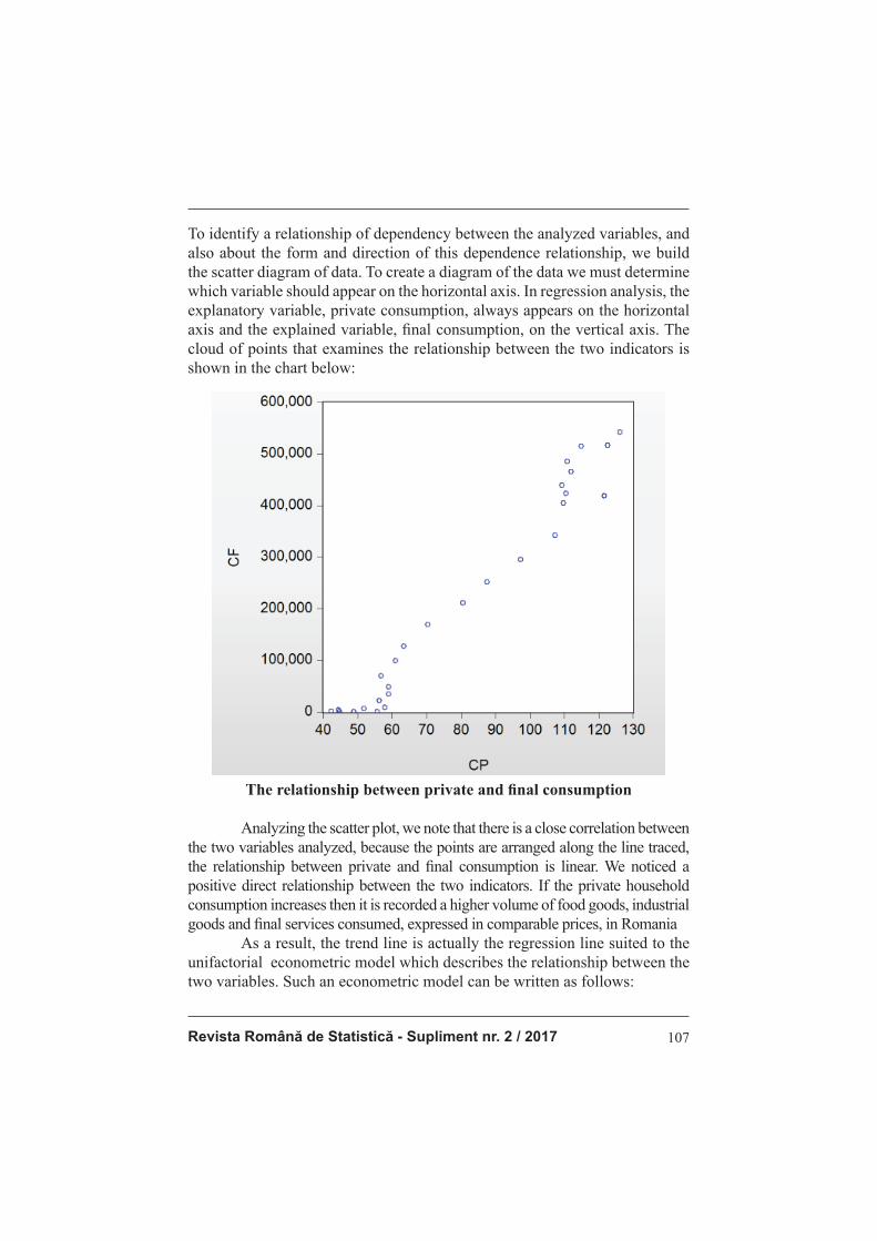
Revista Română de Statistică - Supliment nr. 2 / 2017 107

To identify a relationship of dependency between the analyzed variables, and also about the form and direction of this dependence relationship, we build the scatter diagram of data. To create a diagram of the data we must determine which variable should appear on the horizontal axis. In regression analysis, the explanatory variable, private consumption, always appears on the horizontal axis and the explained variable, fi nal consumption, on the vertical axis. The

cloud of points that examines the relationship between the two indicators is

shown in the chart below:

The relationship between private and fi nal consumption

Analyzing the scatter plot, we note that there is a close correlation between

the two variables analyzed, because the points are arranged along the line traced,

the relationship between private and fi nal consumption is linear. We noticed a

positive direct relationship between the two indicators. If the private household

consumption increases then it is recorded a higher volume of food goods, industrial

goods and fi nal services consumed, expressed in comparable prices, in Romania

As a result, the trend line is actually the regression line suited to the

unifactorial econometric model which describes the relationship between the

two variables. Such an econometric model can be written as follows:

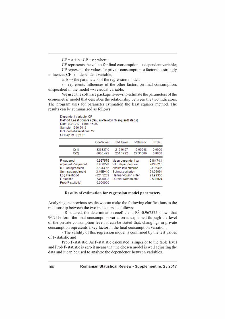
Romanian Statistical Review - Supplement nr. 2 / 2017108

CF = a + b ∙ CP + e ; where:

CF represents the values for fi nal consumption → dependent variable;

CP represents the values for private consumption, a factor that strongly

infl uences CF→ independent variable;

a, b → the parameters of the regression model;

e - represents infl uences of the other factors on fi nal consumption,

unspecifi ed in the model → residual variable.

We used the software package Eviews to estimate the parameters of the

econometric model that describes the relationship between the two indicators.

The program uses for parameter estimation the least squares method. The

results can be summarized as follows:

Results of estimation for regression model parameters

Analyzing the previous results we can make the following clarifi cations to the

relationship between the two indicators, as follows:

- R-squared, the determination coeffi cient, R2=0.967575 shows that

96.75% form the fi nal consumption variation is explained through the level

of the private consumption level; it can be stated that, changings in private

consumption represents a key factor in the fi nal consumption variation;

- The validity of this regression model is confi rmed by the test values

of F-statistic and

Prob F-statistic. As F-statistic calculated is superior to the table level

and Prob F-statistic is zero it means that the chosen model is well adjusting the

data and it can be used to analyze the dependence between variables.

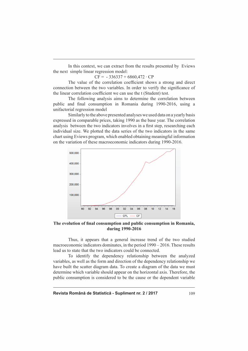
Revista Română de Statistică - Supliment nr. 2 / 2017 109

In this context, we can extract from the results presented by Eviews the next simple linear regression model:

CF = - 336337 + 6860,472 ∙ CP

The value of the correlation coeffi cient shows a strong and direct

connection between the two variables. In order to verify the signifi cance of

the linear correlation coeffi cient we can use the t (Student) test.

The following analysis aims to determine the correlation between

public and fi nal consumption in Romania during 1990-2016, using a

unifactorial regression model

Similarly to the above presented analyses we used data on a yearly basis

expressed in comparable prices, taking 1990 as the base year. The correlation

analysis between the two indicators involves in a fi rst step, researching each

individual size. We plotted the data series of the two indicators in the same

chart using Eviews program, which enabled obtaining meaningful information

on the variation of these macroeconomic indicators during 1990-2016.

The evolution of fi nal consumption and public consumption in Romania,

during 1990-2016

Thus, it appears that a general increase trend of the two studied

macroeconomic indicators dominates, in the period 1990 – 2016. These results

lead us to state that the two indicators could be connected.

To identify the dependency relationship between the analyzed

variables, as well as the form and direction of the dependency relationship we

have built the scatter diagram data. To create a diagram of the data we must

determine which variable should appear on the horizontal axis. Therefore, the

public consumption is considered to be the cause or the dependent variable

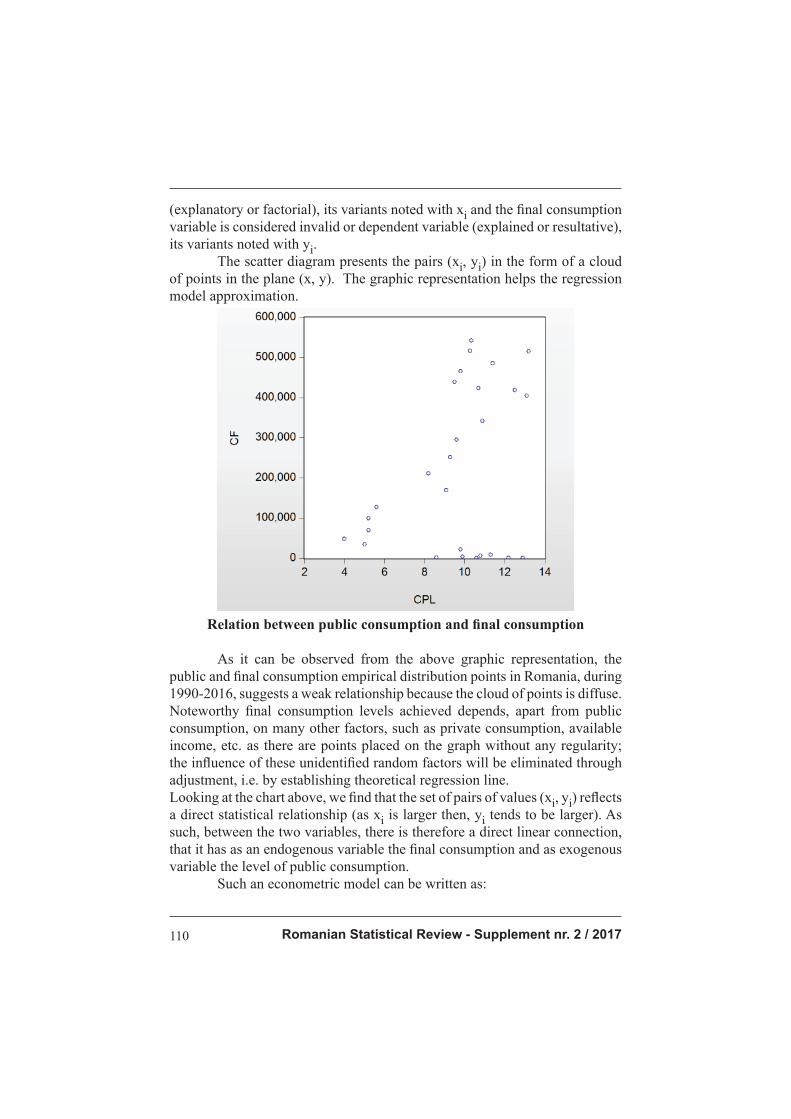
Romanian Statistical Review - Supplement nr. 2 / 2017110

(explanatory or factorial), its variants noted with xi and the fi nal consumption

variable is considered invalid or dependent variable (explained or resultative),

its variants noted with yi.

The scatter diagram presents the pairs (xi, yi) in the form of a cloud

of points in the plane (x, y). The graphic representation helps the regression

model approximation.

Relation between public consumption and fi nal consumption

As it can be observed from the above graphic representation, the

public and fi nal consumption empirical distribution points in Romania, during

1990-2016, suggests a weak relationship because the cloud of points is diffuse.

Noteworthy fi nal consumption levels achieved depends, apart from public

consumption, on many other factors, such as private consumption, available

income, etc. as there are points placed on the graph without any regularity;

the infl uence of these unidentifi ed random factors will be eliminated through

adjustment, i.e. by establishing theoretical regression line.

Looking at the chart above, we fi nd that the set of pairs of values (xi, yi) refl ects

a direct statistical relationship (as xi is larger then, yi tends to be larger). As

such, between the two variables, there is therefore a direct linear connection,

that it has as an endogenous variable the fi nal consumption and as exogenous

variable the level of public consumption.

Such an econometric model can be written as:

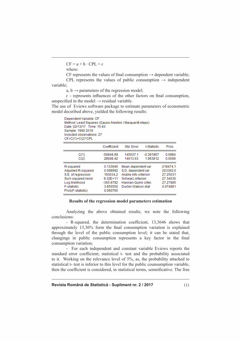
Revista Română de Statistică - Supliment nr. 2 / 2017 111

CF = a + b ∙ CPL + e

where:

CF represents the values of fi nal consumption → dependent variable;

CPL represents the values of public consumption → independent

variable;

a, b → parameters of the regression model;

e - represents infl uences of the other factors on fi nal consumption,

unspecifi ed in the model → residual variable.

The use of Eviews software package to estimate parameters of econometric

model decsribed above, yielded the following results:

Results of the regression model parameters estimation

Analyzing the above obtained results, we note the following

conclusions:

- R-squared, the determination coeffi cient, 13,3646 shows that

approximately 13,36% form the fi nal consumption variation is explained

through the level of the public consumption level; it can be stated that,

changings in public consumption represents a key factor in the fi nal

consumption variation;

- For each independent and constant variable Eviews reports the

standard error coeffi cient; statistical t- test and the probability associated

to it. Working on the relevance level of 5%, as, the probability attached to

statistical t- test is inferior to this level for the public counsumption variable,

then the coeffi cient is considered, in statistical terms, semnifi cative. The free

Romanian Statistical Review - Supplement nr. 2 / 2017112

term coeffi cient is not signifi cant because the probability attached to statistical

t- test is above the threshold of signifi cance 5%; In this context, we can extract from the results presented by Eviews the following simple linear regression model: CF = -56849,69 + 28698,42∙ CPL

The regression coeffi cient positive sign confi rms the above, that there

is a direct connection between the two variables studied.

The correlation coeffi cient value indicates a direct connection, weak

between the two variables. In order to verify the signifi cance of the linear

correlation coeffi cient the t (Student) test can be used.

Conclusions

The fi nal consumption evolution is infl uenced decisively by the private consumption variation, while recording a less sizable impact by the public consumption dynamics. The variation of fi nal consumption in our country it is weak infl uenced by the evolution of public consumption. The high value of the free term refl ects the infl uence of factors which were not taken into account when building the regression models and that contribute signifi cantly on the evolution of fi nal consumption. However the models used, although they are correct and well chosen, can be developed and deepened in order to ensure better outcomes for forecasting.

References

1. Andersen, T., Bollerslev, T., Diebold, F., Labys, P. (2003). Modeling and

Forecasting Realized Volatility, Econometrica, Volume 71, Issue 2, pp. 579–625 2. Anghelache, C., Anghel, M.G. (2016). Econometrie generală. Concepte, teorie și

studii de caz, Editura Artifex, Bucureşti

3. Anghelache, C., Manole, A., Anghel, M.G. (2015). Unifactorial Econometric

Model - Connection between the Final Consumption and the Private Consumption,

Asian Academic Research Journal Of Social Science & Humanities, Volume 2,

Issue 6, November 2015, pp. 212-219

4. Anghelache, C., Anghel, M.G., Popovici, M. (2015). Multiple Regressions Used

in Analysis of Private Consumption and Public Final Consumption Evolution,

International Journal of Academic Research in Accounting, Finance and

Management Sciences, Volume 5, No. 4, October 2015, pp. 69-73

5. Anghelache, C., Manole, A., Dumitrescu, D. (2015). The Correlation between Final

Consumption, Gross Available Income and Gross Investment: An Econometric

Analysis, International Journal of Academic Research in Accounting, Finance and

Management Sciences, Vol. 5, Nr. 4, 2015, pp. 84-88

6. Anghelache, C. (2008). Tratat de statistică teoretică şi economică, Editura

Economică, Bucureşti

Revista Română de Statistică - Supliment nr. 2 / 2017 113

7. Bardsen, G., Nymagen, R., Jansen, E. (2005). The Econometrics of Macroeconomic

Modelling, Oxford University Press 8. Bastagli, F., Hills, J. (2013). What Gives? Household Consumption Patterns

and the‚ Big Trade Off’ with Public Consumption, Centre for Analysis of Social Exclusion, LSE in series CASE Papers with number case170

9. Censolo, R., Colombo, C. (2008). Public consumption composition in

a growingeconomy, Journal of Macroeconomics. Volume (Year): 30 (2008), Issue (Month): 4(December), 1479-1495

10. Dodge, Y. (editor) (2006). The Oxford dictionary of statistical terms, Oxford University Press

11. Foerster, A.T., Choi, J. (2016). Consumption Growth Regimes and the Post-

Financial Crisis Recovery, Economic Review, Volume (Year): (2016), Issue (Month): Q II (), pp. 25-48

12. Hamilton, J., Waggoner, D., Zha, T. (2007). Normalization in econometrics, Econometrics Reviews, nr. 26, pp. 221-252

13. Klein, P., Krusell, P., Rios-Rull, V. (2008). Time-Consistent Public Policy, Review of Economic Studies, 75, pp. 789–808

14. Lohr, S.L. (2007). Comment: Struggles with Survey Weighting and Regression

Modeling, Statistical Science, Vol. 22, No. 2, pp.175–178 15. Lorenzoni, G. (2009). A Theory of Demand Shocks, American Economic Review

99, no. 5, pp. 2050-2084 16. van Eijck, K., Majorana, M. (2013). Consumption patterns, in Ruth Towse &

Christian Handke (ed.), „Handbook on the Digital Creative Economy”, Books, Edward Elgar, number 14906, 6

Romanian Statistical Review - Supplement nr. 2 / 2017114

Model econometric de analiză a corelaţiei dintre produsul intern brut şi consumul fi nal

Conf. univ. dr. Mădălina-Gabriela ANGHEL

Universitatea „ARTIFEX” din Bucureşti Drd. Radu STOICA

Academia de Studii Economice din BucureştiDrd. Tudor SAMSON

Academia de Studii Economice din BucureştiDrd. Alexandru BADIU

Academia de Studii Economice din Bucureşti

Abstract

Consumul fi nal este unul dintre cele mai importante componente ale

modelului structural al PIB-ului României. Defalcat în consum privat şi public, acest indicator oferă o viziune valoroasă asupra înclinaţiei către consum a

populaţiei. De asemenea, măsoară consumul public, o variabilă care este

importantă în analize bugetare. Astfel, infl uenţa consumului fi nal asupra PIB

este unul dintre elementele cheie în analizele macroeconomice.

Cuvinte cheie: PIB, consum fi nal, regresie, parametru, infl uenţă

Clasifi care JEL: E01, E20, E21

Introducere

Analiza infl uenţei consumului fi nal asupra Produsului Intern Brut este una dintre cele mai importante studii care urmează principiile metodei

cheltuielilor de formare şi determinare a PIB. Cu cât este mai complexă

analiza, cu atât sunt mai utile rezultatele obţinute. Abordarea econometrică

oferă rezultate de substanţă atunci când este abordat un interval mai lung

de timp şi unul dintre adevărurile desprinse din modelul econometric este

dependenţa economiei naţionale de consumul fi nal.

Astfel, modelul de regresie unifactorial poate fi utilizat şi pentru

stabilirea infl uenţei pe care o are valoarea consumului fi nal asupra evoluţiei

Produsului Intern Brut al României.

Literature review

Davidson şi Mackinnon (2004), Dougherty (2007), Anghelache şi

Anghel (2016), Andrei şi Spătaru (2010) dezvoltă pe tema instrumentelor

şi aplicaţiilor econometrice. Regresia a fost utilizată ca tehnică de analiză

la nivel macroeconomic, de către Anghelache şi Sacală (2016), Anghelache,

Revista Română de Statistică - Supliment nr. 2 / 2017 115

Soare şi Popovici (2015), Anghelache, Manole, Anghel (2015). Anghelache şi Anghel (2014) este un documentar de referinţă asupra aspectelor teoretice

şi practice ale modelării economice. Censolo şi Colombo (2008) studiază structura consumului public considerând un anume trend al economiei. Chamberlin (2011) dezvoltă asupra interacţiunii dintre PIB şi două măsuri ale bunăstării. Aspecte ale consumului sunt analizate de Colloredo-Mansfeld (2005), Jorgenson şi Slesnick (2008), Reis (2009). Newbold, Karlson şi Thorne (2010) dezvoltă pe tema instrumentelor statistice utile în domeniul economic şi de afaceri. De Michelis şi Monfort (2008) discută despre GDP sub impactul convergenţei regionale şi politicii de coeziune la nivel european. Hassler, Storesletten şi Zilibotti (2007) se concentrează asupra binelui public într-un mediu democratic. Kocherlakota (2010) abordează unele dinamici inovative ale fi nanţelor publice.

Metodologia cercetării şi date. Rezultate şi analiză

Am utilizat date cu o frecvență anuală acoperind perioada 1990-2016, iar pentru a asigura comparabilitatea datelor, valorile celor doi indicatori macroeconomici au fost defl atate folosind în acest sens indicele prețurilor de consum (utilizat de Institutul Național de Statistică pentru a calcula rata infl ației în România), care surprinde evoluția prețurilor bunilor și tarifelor serviciilor fi nale achiziționate de către populație, în anul curent față de anul 1990, ales ca perioadă de referință. Defl atarea datelor s-a realizat prin împărţirea la Indicele Preţului de Consum din anul respectiv a valorilor nominale ale PIB-ului și ale consumului fi nal. În acest sens, am considerat o serie de date cu privire la evoluţia celor doi indicatori macroeconomici menţionaţi anterior, în perioada 1990-2016. Analiza corelaţiei dintre cei indicatori presupune, într-o primă etapă, analiza individuală a fi ecărei mărimi considerate. În ceea ce priveşte evoluţia Produsul Intern Brut în România, seria de date a fost procesată cu ajutorul programului informatic Eviews, ceea ce a permis obţinerea unor informaţii semnifi cative referitoare la variaţia acestui indicator macroeconomic în perioada 1990-2016.

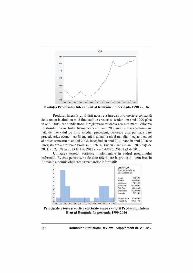
Romanian Statistical Review - Supplement nr. 2 / 2017116

Evoluţia Produsului Intern Brut al României în perioada 1990 - 2016

Produsul Intern Brut al ţării noastre a înregistrat o creştere constantă

de la un an la altul, cu mici fl uctuații de creșteri și scăderi din anul 1990 până în anul 2008, când indicatorul înregistrează valoarea cea mai mare. Valoarea Produsului Intern Brut al României pentru anul 2009 înregistrează o diminuare faţă de intervalul de timp imediat precedent, deoarece este perioada care precede criza economico-fi nanciară instalată la nivel mondial începând cu cel al doilea semestru al anului 2008. Începând cu anul 2011 până în anul 2016 se înregistrează o creștere a Produsului Intern Brut cu 2,16% în anul 2012 față de 2011, cu 2,75% în 2013 față de 2012 și cu 3,49% în 2016 față de 2013. Utilizarea testelor statistice implementate în cadrul programului informatic Eviews pentru seria de date referitoare la produsul intern brut în România a permis obţinerea următoarelor informaţii:

Principalele teste statistice efectuate asupra valorii Produsului Intern

Brut al României în perioada 1990-2016

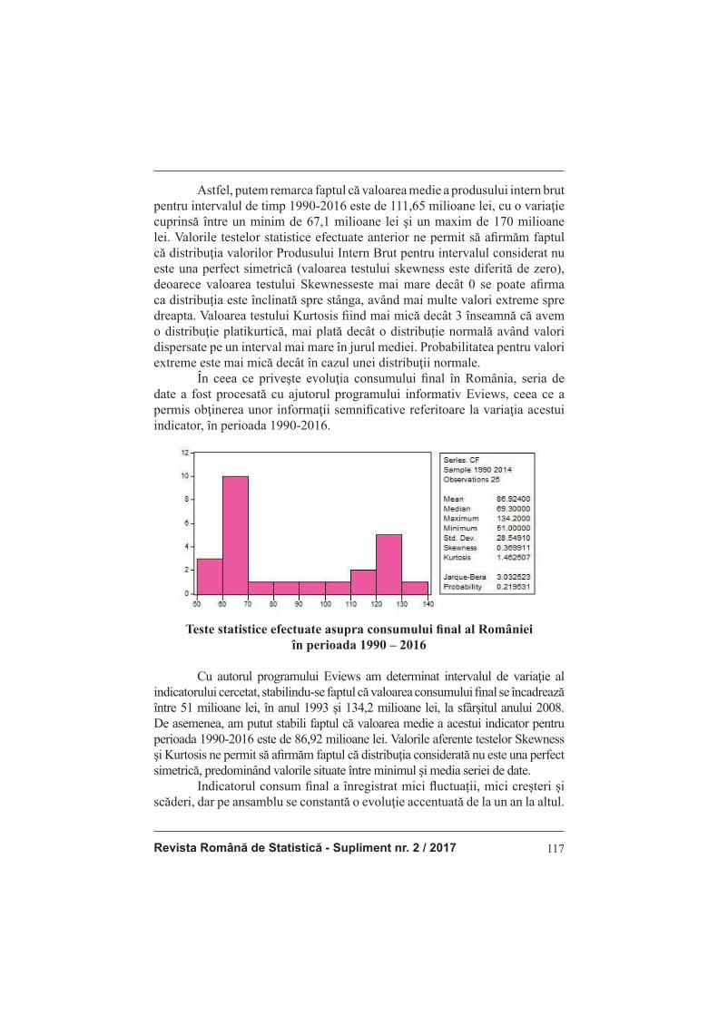
Revista Română de Statistică - Supliment nr. 2 / 2017 117

Astfel, putem remarca faptul că valoarea medie a produsului intern brut pentru intervalul de timp 1990-2016 este de 111,65 milioane lei, cu o variaţie cuprinsă între un minim de 67,1 milioane lei şi un maxim de 170 milioane

lei. Valorile testelor statistice efectuate anterior ne permit să afi rmăm faptul că distribuţia valorilor Produsului Intern Brut pentru intervalul considerat nu este una perfect simetrică (valoarea testului skewness este diferită de zero), deoarece valoarea testului Skewnesseste mai mare decât 0 se poate afi rma ca distribuția este înclinată spre stânga, având mai multe valori extreme spre dreapta. Valoarea testului Kurtosis fi ind mai mică decât 3 înseamnă că avem o distribuţie platikurtică, mai plată decât o distribuție normală având valori dispersate pe un interval mai mare în jurul mediei. Probabilitatea pentru valori extreme este mai mică decât în cazul unei distribuţii normale. În ceea ce priveşte evoluţia consumului fi nal în România, seria de date a fost procesată cu ajutorul programului informativ Eviews, ceea ce a permis obţinerea unor informaţii semnifi cative referitoare la variaţia acestui indicator, în perioada 1990-2016.

Teste statistice efectuate asupra consumului fi nal al României

în perioada 1990 – 2016

Cu autorul programului Eviews am determinat intervalul de variaţie al indicatorului cercetat, stabilindu-se faptul că valoarea consumului fi nal se încadrează între 51 milioane lei, în anul 1993 şi 134,2 milioane lei, la sfârşitul anului 2008. De asemenea, am putut stabili faptul că valoarea medie a acestui indicator pentru perioada 1990-2016 este de 86,92 milioane lei. Valorile aferente testelor Skewness şi Kurtosis ne permit să afi rmăm faptul că distribuţia considerată nu este una perfect simetrică, predominând valorile situate între minimul şi media seriei de date. Indicatorul consum fi nal a înregistrat mici fl uctuații, mici creșteri și scăderi, dar pe ansamblu se constantă o evoluţie accentuată de la un an la altul.

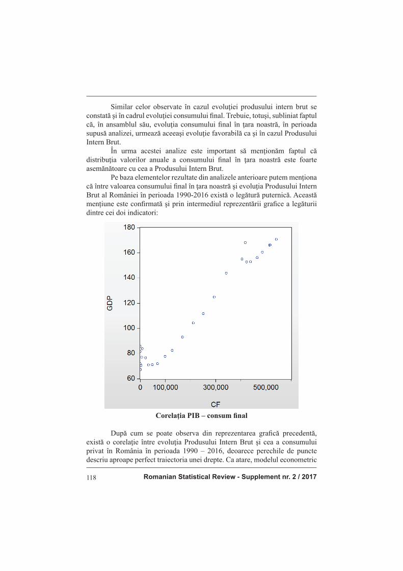
Romanian Statistical Review - Supplement nr. 2 / 2017118

Similar celor observate în cazul evoluţiei produsului intern brut se constată şi în cadrul evoluţiei consumului fi nal. Trebuie, totuşi, subliniat faptul că, în ansamblul său, evoluţia consumului fi nal în ţara noastră, în perioada supusă analizei, urmează aceeaşi evoluţie favorabilă ca şi în cazul Produsului Intern Brut. În urma acestei analize este important să menţionăm faptul că distribuţia valorilor anuale a consumului fi nal în ţara noastră este foarte asemănătoare cu cea a Produsului Intern Brut. Pe baza elementelor rezultate din analizele anterioare putem menționa că între valoarea consumului fi nal în ţara noastră şi evoluţia Produsului Intern Brut al României în perioada 1990-2016 există o legătură puternică. Această mențiune este confi rmată şi prin intermediul reprezentării grafi ce a legăturii dintre cei doi indicatori:

Corelaţia PIB – consum fi nal

După cum se poate observa din reprezentarea grafi că precedentă, există o corelaţie între evoluţia Produsului Intern Brut şi cea a consumului privat în România în perioada 1990 – 2016, deoarece perechile de puncte descriu aproape perfect traiectoria unei drepte. Ca atare, modelul econometric

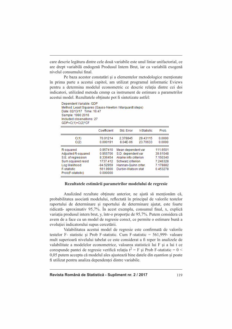
Revista Română de Statistică - Supliment nr. 2 / 2017 119

care descrie legătura dintre cele două variabile este unul liniar unifactorial, ce are drept variabilă endogenă Produsul Intern Brut, iar ca variabilă exogenă nivelul consumului fi nal. Pe baza acestor constatări şi a elementelor metodologice menţionate în prima parte a acestui capitol, am utilizat programul informatic Eviews pentru a determina modelul econometric ce descrie relaţia dintre cei doi indicatori, utilizând metoda cmmp ca instrument de estimare a parametrilor acestui model. Rezultatele obţinute pot fi sintetizate astfel:

Rezultatele estimării parametrilor modelului de regresie

Analizând rezultate obţinute anterior, ne ajută să menționăm că, probabilitatea asociată modelului, refl ectată în principal de valorile testelor raportului de determinare și raportului de determinare ajutat, este foarte ridicată- aproximativ 95,7%. În acest exemplu, consumul fi nal, x, explică variaţia produsul intern brut, y, într-o proporţie de 95,7%. Putem considera că avem de a face cu un model de regresie corect, ce permite o estimare bună a evoluţiei indicatorului supus cercetării. Valabilitatea acestui model de regresie este confi rmată de valorile testelor F- statistic și Prob F-statistic. Cum F-statistic = 561,999- valoare mult superioară nivelului tabelat ce este considerat a fi reper în analizele de valabilitate a modelelor econometrice, valoarea statisticii lui F și a lui t ce corespunde pantei de regresie verifi că relația t2 = F și Prob F-statistic = 0 < 0,05 putem accepta că modelul ales ajustează bine datele din eșantion și poate fi utilizat pentru analiza dependenței dintre variabile.

Romanian Statistical Review - Supplement nr. 2 / 2017120

Pentru fi ecare variabilă independentă şi constantă Eviews raportează eroarea standard a coefi cientului, testul t-Statistic şi probabilitatea asociată acestuia. Lucrând la nivelul de relevanţă de 5%, cum, probabilitatea ataşată testului t-statistic este inferioară acestui nivel pentru CF, atunci coefi cientul este considerat semnifi cativ din punct de vedere statistic. Coefi cientul termenului liber nu este semnifi cativ deoarece probabilitatea ataşată testului t-statistic este mult superioară pragului de semnifi cație de 5%. În acest context, putem extrage din rezultatele prezentate de programul informatic specializat Eviews următorul model de regresie liniară simplă:

PIB = 70.01214+ 0,000191 ∙ FC La creşterea cu un milion lei a consumului fi nal, Produsul Intern Brut

va crește cu 0,000191 milioane lei, de unde reiese existența legăturii directe între cele două variabile studiate. Valoarea coefi cientului de corelaţie indică o legătură directă și de

intensitate mare între cele două variabile.

Concluzii

Produsul Intern Brut este infl uențat în mod hotărâtor de consumul

fi nal. Parametrii modelului de regresie estimat demonstrează că economia

românească din ultimii douăzeci de ani a fost fundamentată aproape

exclusiv pe stimularea consumului şi mai puţin pe promovarea unei politici

investiţionale corecte. Creşterea consumului fi nal este direct corelată cu

creşterea economică, măsurată prin indicatorul macroeconomic- produsul

intern brut. Valoarea termenului liber conduce spre afi rmația că indicatorii

care nu fac parte din acest model de regresie contribuie semnifi cativ asupra

evoluţiei principalului agregat macroeconomic – produsul intern brut.

Bibliografi e

1. Andrei, T., Spătaru, L. (2010). Aplicaţii în econometrie, Editura Economică,

Bucureşti

2. Anghelache, C., Sacală, C. (2016). Multiple linear regression used to analyse

the corelation between GDP and some variables, Romanian Statistical Review,

Supplement, no.9, pp. 94-99

3. Anghelache, C., Anghel, M.G. (2016). Econometrie generală. Concepte, teorie și

studii de caz, Editura Artifex, Bucureşti

4. Anghelache, C., Soare, D.V., Popovici, M. (2015). Analysis of Gross Domestic

Product Evolution under the Infl uence of the Final Consumption, Theoretical and

Applied Economics, Volume XXII, No.4 (605), Winter, pp. 45-52

5. Anghelache, C., Manole, A., Anghel, M.G. (2015). The analysis of the correlation

between GDP, private and public consumption through multiple regression,

Romanian Statistical Review - Supplement, No. 8, pp. 34 – 40

Revista Română de Statistică - Supliment nr. 2 / 2017 121

6. Anghelache, C., Anghel, M. (2014). Modelare economică. Concepte, teorie şi

studii de caz., Editura Economică 7. Censolo, R., Colombo, C. (2008). Public consumption composition in a growing

economy, Journal of Macroeconomics. Volume (Year): 30 (2008), Issue (Month): 4 (December), 1479-1495

8. Chamberlin, G. (2011). Gross domestic product, real income and economic welfare, Economic & Labour Market Review, Volume (Year): 5 (2011), Issue (Month): 5 (May), pp. 5-25

9. Colloredo-Mansfeld, R. (2005). Consumption in James G. Carrier (ed.), 2005. „A Handbook of Economic Anthropology,” Books, Edward Elgar, number 2904, 6

10. Davidson, R., Mackinnon, J.G. (2004). Econometric theory and methods, Oxford University Press, New York

11. De Michelis, N., Monfort, P. (2008). Some refl ections concerning GDP, regional

convergence and European cohesion policy, Regional Science Policy & Practice, Volume (Year): 1 (2008), Issue (Month): 1 (November), pp. 15-22

12. Dougherty, C. (2007). Introduction to Econometrics, Oxford University Press 13. Jorgenson, D., Slesnick, D. (2008). Consumption and Labor Supply, Journal of

Econometrics 147, no. 2 (December 2008), pp. 326-335 14. Hassler, J., Storesletten, K., Zilibotti, F. (2007). Democratic Public Good

Provision, Journal of Economic Theory, 130, 1, pp. 127–151 15. Kocherlakota, N.R. (2010). The New Dynamic Public Finance, Princeton

University Press 16. Newbold, P., Karlson, L.W., Thorne, B. (2010). Statistics for Business and

Economics, 7th ed., Pearson Global Edition, Columbia, U.S. 17. Reis, R. (2009). The Time-Series Properties of Aggregate Consumption:

Implications for the Costs of Fluctuations, Journal of the European Economic Association, 7(4), pp. 722-753

Romanian Statistical Review - Supplement nr. 2 / 2017122

ANALYSIS OF THE ECONOMETRIC MODEL OF THE CORRELATION BETWEEN GDP

AND FINAL CONSUMPTION

Assoc. prof. Mădălina-Gabriela ANGHEL PhD.

„ARTIFEX” University of Bucharest

Radu STOICA PhD. Student

Bucharest University of Economic Studies

Tudor SAMSON PhD. Student

Bucharest University of Economic Studies

Alexandru BADIU PhD. Student

Bucharest University of Economic Studies

Abstract

The fi nal consumption is one of the most important components

of the Romanian GDP structural model. Divided into private and public

consumption, this indicator offers valuable insight especially on the

populations’ determination to consume. Also, it measures the public

consumption, a variable that is important in budgetary analyses. Thus, the

infl uence of the fi nal consumption on the GDP is one of the key topics in

macroeconomic analyses.

Key words: GDP, fi nal consumption, regression, parameter, infl uence

JEL Classifi cation: E01, E20, E21

Introduction

The analysis of the fi nal consumption infl uence on the Gross Domestic

Product is one of the most important studies that follow the expenses method

of GDP calculation and formation. The more complex the analysis, the

more useful the results drawn. The econometric approach gives substantial

results when a longer interval is approached and, one of the truths behind

the econometric model is the dependence of the national economy on fi nal

consumption.

Thus, the unifactorial regression model can be used to establish the

infl uence that the value of fi nal consumption has on the evolution of Romania’s

Gross Domestic Product.

Literature review

Davidson and Mackinnon (2004), Dougherty (2007), Anghelache and

Anghel (2016), Andrei and Spătaru (2010) develop on econometric instruments and applications. The regression has been used as analysis technique at the

Revista Română de Statistică - Supliment nr. 2 / 2017 123

macroeconomic level, by Anghelache and Sacală (2016), Anghelache, Soare and Popovici (2015), Anghelache, Manole, Anghel (2015). Anghelache and Anghel (2014) is a reference document on theoretical and practical aspects of economic modelling. Censolo and Colombo (2008) study the structure of public consumption in a given trend of economy. Chamberlin (2011) develops on the interaction between GDP and two measures of welfare. Various aspects of consumption are analysed by Colloredo-Mansfeld (2005), Jorgenson and Slesnick (2008), Reis (2009). Newbold, Karlson and Thorne (2010) develop on statistics instruments useful in economy and business fi elds. De Michelis and Monfort (2008) discuss on GDP under the impact of regional convergence and cohesion policy at the European level. Hassler, Storesletten and Zilibotti (2007) focus on the public good in a democratic. Kocherlakota (2010) approach innovative dynamics of public fi nance.

Research methodology and data. Results and analysis

We used data on a yearly basis covering the period 1990-2016, and to ensure data comparability, the values of the two macroeconomic indicators were defl ated using the consumer price index ( used by the National Institute of Statistics to calculate the infl ation rate in Romania), which captures the evolution of asset prices and fi nal rates purchased by the population in the current year compared to 1990, mainly as a reference. Defl ating the data was performed by dividing the Consumer Price Index from that year of the denominations of GDP and fi nal consumption. For this purpose, we considered a number of data regarding the evolution of the two macroeconomic indicators mentioned before, during 1990-2016. Correlation analysis of the indicators involves at fi rst stage, an individual analysis of each size. Regarding the evolution of GDP in Romania, the data set was processed using Eviewsprogram, which enabled the obtaining of meaningful information about the fl uctuation of the macroeconomic indicators during 1990-2016.

Romanian Statistical Review - Supplement nr. 2 / 2017124

The GDP evolution in Romania between 1990 – 2016

The GDP of our country recorded a steady growth from year to year, with small fl uctuations increases and decreases from 1990 to 2008, when the indicator recorded the highest value. The value of Romania’s GDP for 2009 has recorded a decrease compared to the immediately preceding time, because is the period that precedes the fi nancial and economic crisis installed world-wide starting the second semester of 2008. From 2011 until 2016 is recorded an increase of the GDP with 2,16% in 2012 compared to 2011, with 2.75% in 2013 compared to 2012 and by 3.49% in 2016 to 2013. Using statistical tests implemented in the software Eviews for the data series regarding GDP in Romania, has allowed us to obtain the following information:

Main statistical tests made on the value of the GDP in Romania 1990-2016

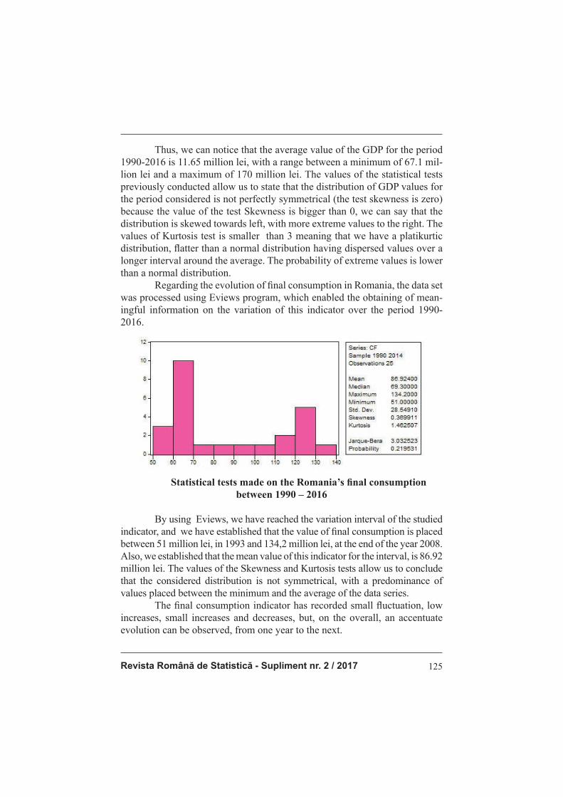
Revista Română de Statistică - Supliment nr. 2 / 2017 125

Thus, we can notice that the average value of the GDP for the period 1990-2016 is 11.65 million lei, with a range between a minimum of 67.1 mil-lion lei and a maximum of 170 million lei. The values of the statistical tests previously conducted allow us to state that the distribution of GDP values for the period considered is not perfectly symmetrical (the test skewness is zero) because the value of the test Skewness is bigger than 0, we can say that the distribution is skewed towards left, with more extreme values to the right. The values of Kurtosis test is smaller than 3 meaning that we have a platikurtic distribution, fl atter than a normal distribution having dispersed values over a longer interval around the average. The probability of extreme values is lower than a normal distribution. Regarding the evolution of fi nal consumption in Romania, the data set was processed using Eviews program, which enabled the obtaining of mean-ingful information on the variation of this indicator over the period 1990-2016.

Statistical tests made on the Romania’s fi nal consumption

between 1990 – 2016

By using Eviews, we have reached the variation interval of the studied indicator, and we have established that the value of fi nal consumption is placed between 51 million lei, in 1993 and 134,2 million lei, at the end of the year 2008. Also, we established that the mean value of this indicator for the interval, is 86.92 million lei. The values of the Skewness and Kurtosis tests allow us to conclude that the considered distribution is not symmetrical, with a predominance of values placed between the minimum and the average of the data series. The fi nal consumption indicator has recorded small fl uctuation, low

increases, small increases and decreases, but, on the overall, an accentuate

evolution can be observed, from one year to the next.

Romanian Statistical Review - Supplement nr. 2 / 2017126

Similar to the facts observed for the evolution of the Gross Domestic Products are the observations on the fi nal consumption. It must be outlined,

however, that the general evolution of the fi nal consumption in our country,

during the period analyzed, follows the same favorable evolution as the Gross

Domestic Product.

Following this analysis is important to note that the annual distributions

of fi nal consumption in our country is very similar to that of the GDP.

Based on the results of the previous analysis, we can mention that

between the fi nal consumption in our country and the evolution of GDP in the

period 1990-2016 there is a strong connection. This statement is confi rmed

through the graphical representation of the connection between the two indi-

cators:

Correlation GDP – Final Consumption

As noticed from the preceding graphic representation, it is a correlation

between changes in GDP and the private consumption in Romania during 1990

– 2016, because the pair of points describes almost perfectly the trajectory of

a straight line. As such, the econometric model that describes the connection

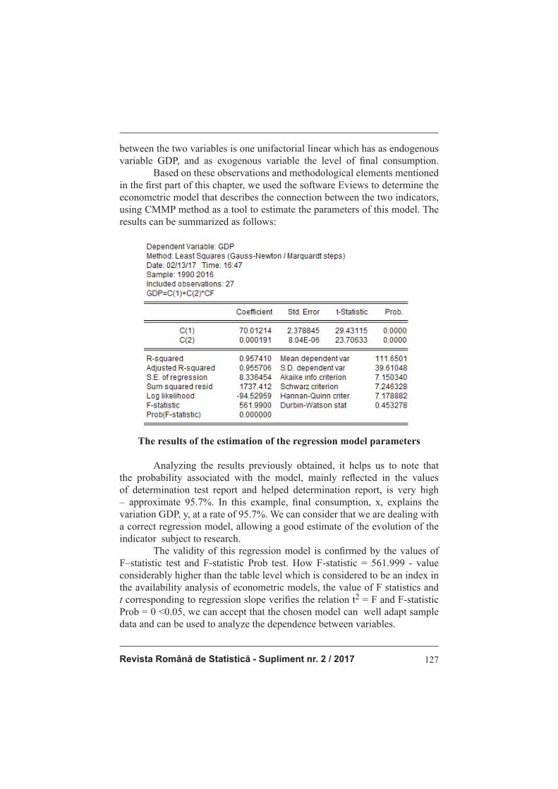
Revista Română de Statistică - Supliment nr. 2 / 2017 127

between the two variables is one unifactorial linear which has as endogenous variable GDP, and as exogenous variable the level of fi nal consumption.

Based on these observations and methodological elements mentioned

in the fi rst part of this chapter, we used the software Eviews to determine the

econometric model that describes the connection between the two indicators,

using CMMP method as a tool to estimate the parameters of this model. The

results can be summarized as follows:

The results of the estimation of the regression model parameters

Analyzing the results previously obtained, it helps us to note that

the probability associated with the model, mainly refl ected in the values

of determination test report and helped determination report, is very high

– approximate 95.7%. In this example, fi nal consumption, x, explains the

variation GDP, y, at a rate of 95.7%. We can consider that we are dealing with

a correct regression model, allowing a good estimate of the evolution of the

indicator subject to research.

The validity of this regression model is confi rmed by the values of

F–statistic test and F-statistic Prob test. How F-statistic = 561.999 - value

considerably higher than the table level which is considered to be an index in

the availability analysis of econometric models, the value of F statistics and

t corresponding to regression slope verifi es the relation t2 = F and F-statistic

Prob = 0 <0.05, we can accept that the chosen model can well adapt sample

data and can be used to analyze the dependence between variables.

Romanian Statistical Review - Supplement nr. 2 / 2017128

For each independent and constant variable and Eviews reports the standard value of the coeffi cient, t-Statistic test and the probability associated

with it.

Working at 5% level of relevance, as the probability attached to t-statistic test is lower to this level for fi nal consumption, then the coeffi cient

is considered statistically signifi cant. Free term coeffi cient is not signifi cant

because the probability attached to t-statistic test is far above the threshold of

5%. In this context, we can excerpt from the results presented by special-ized software Eviews following the simple linear regression model:

GDP = 70.01214+ 0.000191 ∙ FC

Thus, we can say that with the increase with one million lei of fi nal

consumption, GDP will grow by 0.000191 million lei, hence the existence of

a direct link between the two variables studied.

The correlation coeffi cient indicates a direct and high intensity con-

nection between the two variables.

Conclusions

GDP is infl uenced decisively by the fi nal consumption. The param-eters of the estimated regression model demonstrate that the Romanian econ-omy in the last twenty years has been based almost exclusively on stimulat-ing consumption and less on promoting an accurate investment policy. Final consumption growth is directly correlated with economic growth, measured by the macroeconomic indicator - GDP. The elevated value of the constant term leads to the assertion that the indicators that are not part of this regres-sion model contributes in a signifi cant manner on the evolution of the main macroeconomic aggregate - GDP.

References

1. Andrei, T., Spătaru, L. (2010). Aplicaţii în econometrie, Editura Economică,

Bucureşti

2. Anghelache, C., Sacală, C. (2016). Multiple linear regression used to analyse

the corelation between GDP and some variables, Romanian Statistical Review,

Supplement, no.9, pp. 94-99

3. Anghelache, C., Anghel, M.G. (2016). Econometrie generală. Concepte, teorie și

studii de caz, Editura Artifex, Bucureşti

4. Anghelache, C., Soare, D.V., Popovici, M. (2015). Analysis of Gross Domestic

Product Evolution under the Infl uence of the Final Consumption, Theoretical and

Applied Economics, Volume XXII, No.4 (605), Winter, pp. 45-52

5. Anghelache, C., Manole, A., Anghel, M.G. (2015). The analysis of the correlation

between GDP, private and public consumption through multiple regression,

Romanian Statistical Review - Supplement, No. 8, pp. 34 – 40

Revista Română de Statistică - Supliment nr. 2 / 2017 129

6. Anghelache, C., Anghel, M. (2014). Modelare economică. Concepte, teorie şi

studii de caz., Editura Economică 7. Censolo, R., Colombo, C. (2008). Public consumption composition in a growing

economy, Journal of Macroeconomics. Volume (Year): 30 (2008), Issue (Month): 4 (December), 1479-1495

8. Chamberlin, G. (2011). Gross domestic product, real income and economic welfare, Economic & Labour Market Review, Volume (Year): 5 (2011), Issue (Month): 5 (May), pp. 5-25

9. Colloredo-Mansfeld, R. (2005). Consumption in James G. Carrier (ed.), 2005. „A Handbook of Economic Anthropology,” Books, Edward Elgar, number 2904, 6

10. Davidson, R., Mackinnon, J.G. (2004). Econometric theory and methods, Oxford University Press, New York

11. De Michelis, N., Monfort, P. (2008). Some refl ections concerning GDP, regional

convergence and European cohesion policy, Regional Science Policy & Practice, Volume (Year): 1 (2008), Issue (Month): 1 (November), pp. 15-22

12. Dougherty, C. (2007). Introduction to Econometrics, Oxford University Press 13. Jorgenson, D., Slesnick, D. (2008). Consumption and Labor Supply, Journal of

Econometrics 147, no. 2 (December 2008), pp. 326-335 14. Hassler, J., Storesletten, K., Zilibotti, F. (2007). Democratic Public Good

Provision, Journal of Economic Theory, 130, 1, pp. 127–151 15. Kocherlakota, N.R. (2010). The New Dynamic Public Finance, Princeton

University Press 16. Newbold, P., Karlson, L.W., Thorne, B. (2010). Statistics for Business and

Economics, 7th ed., Pearson Global Edition, Columbia, U.S. 17. Reis, R. (2009). The Time-Series Properties of Aggregate Consumption:

Implications for the Costs of Fluctuations, Journal of the European Economic Association, 7(4), pp. 722-753

Romanian Statistical Review - Supplement nr. 2 / 2017130

The Contribution of Higher Education to the Accumulation of Human Capital

in the Romanian Architecture Field During Communism

Valentin Maier

University of Bucharest

Abstract

This article evaluates the contribution of higher education to the

accumulation of human capital in the Romanian architecture domain of activity

during the communist regime. Based on statistical data, legislative acts and

archival documents from National Institute of Statistics, National Archives as

well as other sources, a reconstruction of the accumulation of specialists in

the architecture fi eld is attempted, from presenting the corresponding higher

education organization to types of specialists trained, number of graduates,

constraints and other important aspects not only for architecture, but also for

the evolution of higher education during the communist regime. The architects

and sub-architects, were the two type of specialist trained in the higher

education system, the latter closely resembling the characteristics of sub-

engineers and dentists. Between 1948-1989 there was a period of important

accumulation of specialists for architecture fi eld, especially in 1970s, mostly

due to the introducing of short term education, and with a highest number of

specialist graduating in 1975. Beside this new type of specialist trained from

the beginning of 1970s, the sub-architect, after last of them graduated and

from the middle of 1980s, architects were trained for the fi rst time at evening

form of education, attending 7 years of studies, the longest study time in the

Romanian higher education. All these specialists were trained at “Ion Mincu”

Institute of Architecture from Bucharest, and at sections of architecture

(only for sub-architects) at polytechnics institutes from Iași, Cluj-Napoca

and Timișoara. Although the architecture higher education is not a complex

type of education in terms of presenting its evolution, the contribution to the

accumulation of human capital in the architecture domain of activity was

not an easy task and not only because of the missing statistical data. The

introduction of sub-architects education revealed many interesting aspects of

the process of training specialists through the higher education.

Keywords: Romania, communism, human capital, higher education,

architecture, statistics, graduates.

Revista Română de Statistică - Supliment nr. 2 / 2017 131

After 1948, the communist regime reorganized, according to its ideology, many different aspects of society, including the organization of human settlements. In this respect, it planned and executed important measures, all under complex and long-term process called settlement systematization. This process was presented to the people as a mean to facilitate the social and economical progress, to contribute to the well-being of the people in general. As there are already some studies related to the general architectural changes in the communist Romania, dating both from the communist period and after 1989, we fi nd that an important contribution still is left to be done,

that regarding the specialists meant to implement all the architecture and

systematization projects envisaged by the communist leaders. There are many

questions that need to be answered about them and in this paper we try to

cover some of them, and especially assess the contribution of higher education

to the accumulation of human capital in the architecture fi eld. Also, the case of

architecture higher education is interesting for exemplifying some aspects of

the development of the Romanian higher education in the communist period.

Statistical data, legislative acts and archival documents are the main sources

for this study, and they were consulted at the National Archives of Romania

and National Institute of Statistics, and they were cross-referenced with other

sources.

A few aspects regarding the organization of architecture higher

education need to be presented. Following the Educational Reform from 1948

[1], a new network of institutions of higher education was organized, and in its

structure it also functioned the Institute of Architecture from Bucharest (later

named “Ion Mincu”) [2], with one faculty (bearing different names throughout

the communist period - Architecture, Architecture and Urbanism, Architecture

and Systematization) and with 5 years of studies (later changed to 6) [3], fi rst

under the guidance of State Committee for Architecture and Construction

and not Ministry of Education, like other institutions did at the time of their

foundations (though not a singular example). Later, the institutions of higher

education would all enter the coordination of Ministry of Education and

from 1972 under a double subordination – for Institute of Architecture from

Bucharest and three architecture sections established in 1970 it meant State

Committee for Economy and Local Management [4].

The mentioned architecture sections represent the second most

important milestone in the evolution of architecture higher education. These

sections entered the structure of Faculty of Construction from Polytechnics

Institutes from Iași, Cluj-Napoca and Timișoara. Each section of architecture was structured in departments. For example, in Cluj-Napoca, there were two such departments: Architecture and Theory and History of Architecture and

Romanian Statistical Review - Supplement nr. 2 / 2017132

Urbanism [5]. Although there were some measures planned for training also architects in Iași, Cluj-Napoca and Timișoara [6], they never materialized, and even worse, all the sections were disbanded after 1983, as we will see in the following pages. Their main purpose was to train a new type of specialist for the architecture fi eld in the framework of the (re)introduced sub-engineers education (this time at a level of higher education) [7]. This measure, prepared for a couple of years before and taken in 1968 had effects in the academic year 1968/1969. Three types of specialists were trained in this short term education (less studying time, in general, with 3 years of study, as opposed to 5 or 6 years): sub-engineers of different specializations, sub-architects and dentists. For the architecture fi eld this meant that from the academic year 1970/1971 [8], two type of specialists were important: architects and the newly, sub-architects. The difference between architects (“arhitecți”) and sub-architects

(“conductori arhitecți”) is similar to that from engineers and sub-engineers

(“subingineri”) or from stomatologists (“medici stomatologi”) and dentists

(“medici dentiști”). The education for training sub-engineers, dentists and “conductori arhitecți” was introduced in order to have graduates in the respective fi elds in a quicker time (3 instead of 6 years for architecture) to solve the needs for specialists. As for the name “conductori-arhitecți”, for a easily further reading, we follow the term used by Jan Sadlak, “sub-architects” [9], in analogy with sub-engineers. With the exception of sub-engineers education, all other short forms of education functioned for a brief time: 3 years in the 1970s for the training of dentists [10] and from 1970 to 1983 for sub-architects). With the introducing of the domains of specializations in 1974, another difference appeared, in that architects were trained at architecture and systematization specialization, and sub-architects at architecture specialization, but both in the structure of architecture domain of specializations [11]. In its conception, a sub-architect was to ,,be able to independently assume (not with help from architect), the tasks of a good builder and designer, using current techniques and prefabricated products, for investments limited by his specialization and capability: towns and villages missing specialized help in these problems. Thus, working together with agronomist and doctors, the local administration will propose solutions not only for the completion of different buildings, but also in the overall organization of the respective settlement: housing, production sites, community centres, schools, roads, parks, sport courts. The sub-architect will be used to lead the construction

Revista Română de Statistică - Supliment nr. 2 / 2017 133

works in municipal organization, for management and maintenance” [12]. In the Romanian higher education, the training sub-architects represented a novelty in the way it was done, because a new type of education was introduced, the “învățământ în trepte” (2 stages of education), meaning that after 3 years of study, the worthy students continued their studies in order to become architects, while the other stopped, and graduated as sub-architects. The difference between the two forms of education involves many other considerations that further studies need to solve (the socials implications and the statutes of these graduates as opposed to the “full-time specialists” at their working place, the differences in payment, the rates of trained sub-engineers and engineers, access to the career development, even implications regarding the statutes as intellectuals or not) [13]. This is more important since between architects there were some differences. For example, a graduate of “Ion Mincu” Institute of Architecture from Bucharest allocated to the enterprise Electrouzinproiect in the 1970s said that ,,especially the females are not invested with trust in institutions where they are allocated. Often, there is the bias that females do not have the calling to professions like architecture, engineering. Albeit we, in faculty, receive the same multilateral training as our colleagues, latter followed by specialization in the fi rst years at the working place, there are multiple mistrusts to our quality of work and also to our training received in faculty. These are often not justifi ed” [14]. About the status of sub-engineers it must be said that the Law of Education from 1968 considered sub-engineers education as higher education, mentioning that ,,for the training of middle staff between technicians and foremen are organized, in the structure of polytechnics and technical institutes, sub-engineers and sub-architects sections” (in fact, introduced in 1970) [15] and the same was the case of the Law from 1978 [16]. When studying the wages received by architects and sub-architects, we have to mention that a difference existed. The Law no. 12/1971 regarding the allocation and promotion in work of personnel from socialist state units does not consider sub-engineer education as higher education [17], placing sub-engineer specialists between technicians-foremen and engineers, while in the Law 57/1974 (of remuneration by quantity and quality of labor), a difference in payment existed between engineers and sub-engineers, but also between sub-engineers (considered to have higher education studies, and not in the way of ante-1948 period) and technicians or foremen [18]. Thus, we can appreciate that sub-engineers had higher education studies and wages closer to technicians and foremen. Was the training of sub-architects a bad social-engineering experiment or a successful one, where its success has nothing to do with the duration of this form of

Romanian Statistical Review - Supplement nr. 2 / 2017134

education, as in the case of didactical staff trained in the pedagogical institutes during 1960s? Will try to give an answer after analyzing the statistical data. The last important moment in the history of architecture higher education was the introducing of study place to architects at evening studies in 1979 at “Ion Mincu” Institute of Architecture from Bucharest. These students were to attend 7 years of higher education, a record for the Romanian higher education. The admission for evening studies was constrained by having a working place in the architecture fi eld [19], so it is a clear targeted measure.

Many other interesting facts about the characteristics and evolution

of specialists for the architecture fi eld will be stressed in the following pages,

when presenting and analysing the corresponding statistical data.

In reconstructing the accumulation of human capital in the architecture

fi eld in the communist period we will use statistical data from the Archive of

National Institute of Statistics [20]. We will start by fi nding exactly how many

graduates of architecture higher education resulted in the communist period

(architects and sub-architects):

The number of graduates of architecture higher education

Table 1

Year T F M Year T F M Year T F M

1952 57 n.d. n.d. 1965 134 44 90 1978 448 195 253

1953 56 n.d. n.d. 1966 179 63 116 1979 368 121 247

1954 62 n.d. n.d. 1967 219 102 117 1980 301 109 192

1955 69 29 40 1968 183 88 95 1981 303 96 207

1956 60 20 40 1969 191 104 87 1982 311 131 180

1957 125 n.d. n.d. 1970 204 112 92 1983 255 84 171

1958 120 n.d. n.d. 1971 205 112 93 1984 154 50 104

1959 123 53 70 1972 352 160 192 1985 196 70 126

1960 161 53 108 1973 n.d. n.d. n.d. 1986 193 51 142

1961 100 46 54 1974 498 163 335 1987 147 36 111

1962 84 37 47 1975 554 305 249 1988 125 42 83

1963 60 14 46 1976 457 170 287 1989 n.d. n.d. n.d.

1964 61 21 40 1977 432 188 244

T=total number of graduates; F=female graduates; M=male graduates; n.d.=no data.

There are some mentions that need to be done. First, we do not have

data for some years (1948-1951, 1973 and 1989) and no data for female-male

graduates rate between 1952-1954 and for 1957 and 1958. Although the set of

data is important and even if we had data for all the mentioned years, it would

have represented only the total number of specialists trained in communism,

not the total number of active (working) architects, some of them been trained

before 1948. Also, the data represents the total number of graduates from

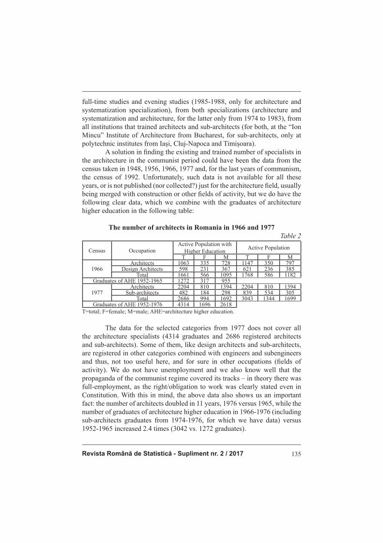
Revista Română de Statistică - Supliment nr. 2 / 2017 135

full-time studies and evening studies (1985-1988, only for architecture and systematization specialization), from both specializations (architecture and systematization and architecture, for the latter only from 1974 to 1983), from all institutions that trained architects and sub-architects (for both, at the “Ion Mincu” Institute of Architecture from Bucharest, for sub-architects, only at polytechnic institutes from Iași, Cluj-Napoca and Timișoara). A solution in fi nding the existing and trained number of specialists in the architecture in the communist period could have been the data from the census taken in 1948, 1956, 1966, 1977 and, for the last years of communism, the census of 1992. Unfortunately, such data is not available for all these years, or is not published (nor collected?) just for the architecture fi eld, usually being merged with construction or other fi elds of activity, but we do have the following clear data, which we combine with the graduates of architecture higher education in the following table:

The number of architects in Romania in 1966 and 1977

Table 2

Census OccupationActive Population with

Higher EducationActive Population

T F M T F M

1966Architects 1063 335 728 1147 350 797

Design Architects 598 231 367 621 236 385Total 1661 566 1095 1768 586 1182

Graduates of AHE 1952-1965 1272 317 955

1977Architects 2204 810 1394 2204 810 1394

Sub-architects 482 184 298 839 534 305Total 2686 994 1692 3043 1344 1699

Graduates of AHE 1952-1976 4314 1696 2618T=total; F=female; M=male; AHE=architecture higher education.

The data for the selected categories from 1977 does not cover all the architecture specialists (4314 graduates and 2686 registered architects and sub-architects). Some of them, like design architects and sub-architects, are registered in other categories combined with engineers and subengineers and thus, not too useful here, and for sure in other occupations (fi elds of activity). We do not have unemployment and we also know well that the propaganda of the communist regime covered its tracks – in theory there was full-employment, as the right/obligation to work was clearly stated even in Constitution. With this in mind, the above data also shows us an important fact: the number of architects doubled in 11 years, 1976 versus 1965, while the number of graduates of architecture higher education in 1966-1976 (including sub-architects graduates from 1974-1976, for which we have data) versus 1952-1965 increased 2.4 times (3042 vs. 1272 graduates).

Romanian Statistical Review - Supplement nr. 2 / 2017136

One more set of data from 1977’s census, the economic branches in which architects worked, registered architects working in three main fi elds, as

structured by the census: other types of fi elds (not industry, agriculture, health

system and others), with 1045 architects working, while the other two most

important were administration and constructions. The sub-architects worked

predominantly in the same main fi eld as architects (census category ”other

types”), in industry, as a second most important employment category and

in construction. This is somehow a correspondance between type of higher

education attended and the later working job.

Unfortunately, as said, the data from the other census is not that relevant

for the architecture fi eld. The reconstruction of the accumulation of human

capital is not helped by the publication Annual Statistics on National Institute

of Statistics, since the fi rst series of data we have presented (for graduates)

is the basis for this annual publication. Also, in 1994 and 1996, there were

two specialized publications for the statistics of educational system, but they

are not helpful either, as the graduates of architecture are included fi rst in the

general technical fi eld, and then combined with construction [21].

Fortunately, we have another series of data from an archival document

with the situation of the working staff with higher education on March 31,

1987 [22]. From this document we found 2743 architects working and 1382

sub-architects, most of them having under 40 years (1536 architects, 1034 sub-

architects). Most of the mentioned specialist were trained during communist

regime. If we compare the total number of specialists working as architects

and sub-architects, meaning 4125 from a total of 640933 working staff (less

than 1%), with the total number of graduates, 7547 (with missing data for 1948-1951, 1973 and 1989) then it means that not all graduates of architecture higher education are working? A solving to this problem is in the way of defi ning the statistical indicators used in this document and especially the

strict “working staff” category, because specialists of architecture could also

had administration and management job (document misses this guideline). We

need more information and data to completely solve this problem, but maybe

new sets of data will be available in the future from the National Archives of

Romania (from the fund State Planning Committee) and other sources.

Although we do not have complete data, we can still easily assess that

the 1970s was the most important period for the accumulation of human capital

in the architecture fi eld (84 graduates in average in 1950s, 137 in 1960s, 390

in 1970s and 220 in 1980s). Also, in 1975 were accounted the most graduates

of the architecture higher education: 554 (see Table 1).

This was facilitated from the year 1970 by the measure to train faster

a new type of specialists to help in resolving the needs of the architecture

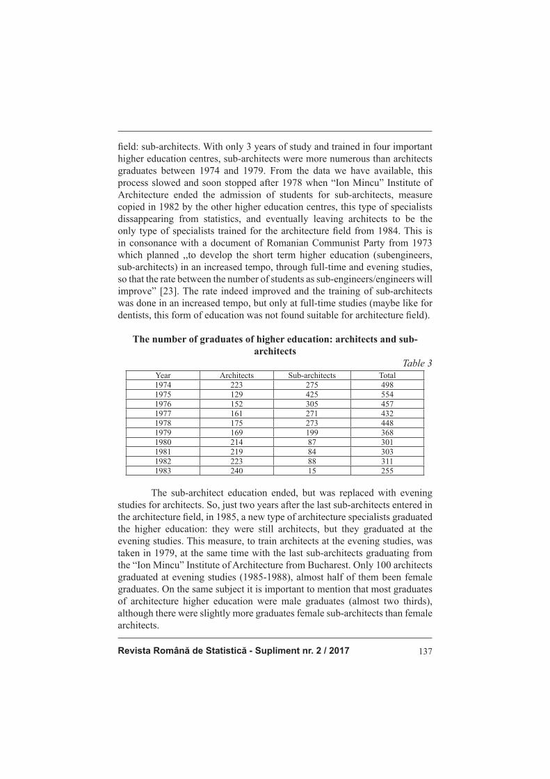
Revista Română de Statistică - Supliment nr. 2 / 2017 137

fi eld: sub-architects. With only 3 years of study and trained in four important

higher education centres, sub-architects were more numerous than architects

graduates between 1974 and 1979. From the data we have available, this

process slowed and soon stopped after 1978 when “Ion Mincu” Institute of

Architecture ended the admission of students for sub-architects, measure

copied in 1982 by the other higher education centres, this type of specialists

dissappearing from statistics, and eventually leaving architects to be the

only type of specialists trained for the architecture fi eld from 1984. This is

in consonance with a document of Romanian Communist Party from 1973

which planned ,,to develop the short term higher education (subengineers,

sub-architects) in an increased tempo, through full-time and evening studies,

so that the rate between the number of students as sub-engineers/engineers will

improve” [23]. The rate indeed improved and the training of sub-architects

was done in an increased tempo, but only at full-time studies (maybe like for

dentists, this form of education was not found suitable for architecture fi eld).

The number of graduates of higher education: architects and sub-

architects

Table 3

Year Architects Sub-architects Total1974 223 275 4981975 129 425 5541976 152 305 4571977 161 271 4321978 175 273 4481979 169 199 3681980 214 87 3011981 219 84 3031982 223 88 3111983 240 15 255

The sub-architect education ended, but was replaced with evening

studies for architects. So, just two years after the last sub-architects entered in

the architecture fi eld, in 1985, a new type of architecture specialists graduated

the higher education: they were still architects, but they graduated at the

evening studies. This measure, to train architects at the evening studies, was

taken in 1979, at the same time with the last sub-architects graduating from

the “Ion Mincu” Institute of Architecture from Bucharest. Only 100 architects

graduated at evening studies (1985-1988), almost half of them been female

graduates. On the same subject it is important to mention that most graduates

of architecture higher education were male graduates (almost two thirds),

although there were slightly more graduates female sub-architects than female

architects.

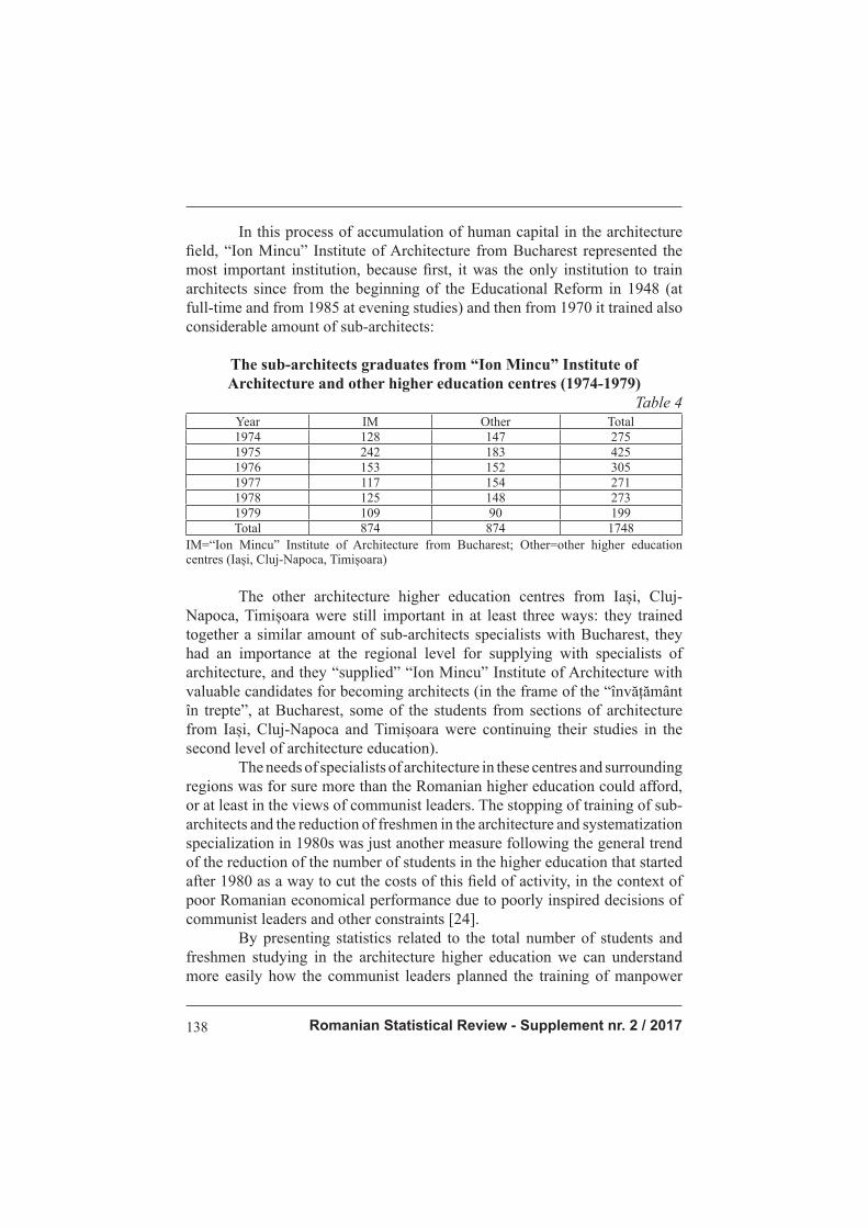
Romanian Statistical Review - Supplement nr. 2 / 2017138

In this process of accumulation of human capital in the architecture fi eld, “Ion Mincu” Institute of Architecture from Bucharest represented the

most important institution, because fi rst, it was the only institution to train

architects since from the beginning of the Educational Reform in 1948 (at

full-time and from 1985 at evening studies) and then from 1970 it trained also

considerable amount of sub-architects:

The sub-architects graduates from “Ion Mincu” Institute of

Architecture and other higher education centres (1974-1979)

Table 4

Year IM Other Total

1974 128 147 275

1975 242 183 425

1976 153 152 305

1977 117 154 271

1978 125 148 273

1979 109 90 199

Total 874 874 1748

IM=“Ion Mincu” Institute of Architecture from Bucharest; Other=other higher education centres (Iași, Cluj-Napoca, Timișoara)

The other architecture higher education centres from Iași, Cluj-Napoca, Timișoara were still important in at least three ways: they trained together a similar amount of sub-architects specialists with Bucharest, they had an importance at the regional level for supplying with specialists of architecture, and they “supplied” “Ion Mincu” Institute of Architecture with valuable candidates for becoming architects (in the frame of the “învățământ în trepte”, at Bucharest, some of the students from sections of architecture from Iași, Cluj-Napoca and Timișoara were continuing their studies in the second level of architecture education). The needs of specialists of architecture in these centres and surrounding regions was for sure more than the Romanian higher education could afford, or at least in the views of communist leaders. The stopping of training of sub-architects and the reduction of freshmen in the architecture and systematization specialization in 1980s was just another measure following the general trend of the reduction of the number of students in the higher education that started after 1980 as a way to cut the costs of this fi eld of activity, in the context of

poor Romanian economical performance due to poorly inspired decisions of

communist leaders and other constraints [24].

By presenting statistics related to the total number of students and

freshmen studying in the architecture higher education we can understand

more easily how the communist leaders planned the training of manpower

Revista Română de Statistică - Supliment nr. 2 / 2017 139

in this fi eld of activity. A close to complete set of data we have from 1960 to

1989. When data was not available we have approximated: for 1970 the data

is obtained with a simple (and satisfactory only because of the missing data)

average result between 1969 and 1971 and for 1971 and 1972 the data is only

for “Ion Mincu” Institute of Architecture from Bucharest and not from the

other institutes, with implication regarding the real number of sub-architects

and total students.

The total number of enlisted students in the architecture higher

education

Table 5

YearStudents

Total Architects Sub-architectsT F M T F M T F M

1960 607 140 467 607 140 467 - - -1961 706 260 446 706 260 446 - - -1962 810 309 501 810 309 501 - - -1963 921 354 567 921 354 567 - - -1964 1069 467 602 1069 467 602 - - -1965 1220 553 767 1220 553 767 - - -1966 1280 625 655 1280 625 655 - - -1967 1284 652 632 1284 652 632 - - -1968 1270 613 657 1270 613 657 - - -1969 1284 604 680 1284 604 680 - - -1970 1242 540 702 1049 470 579 n.d. n.d. n.d.1971 1200 477 723 815 336 479 204 68 1361972 1188 454 734 597 229 368 591 225 3661973 1808 745 1063 546 198 348 1262 574 6881974 1720 730 990 513 199 314 1207 531 6761975 1562 685 877 446 193 253 1116 492 6241976 1485 575 910 495 249 246 990 326 6641977 1561 611 950 718 341 377 843 270 5731978 1693 646 1047 1111 452 659 582 194 3881979 1754 611 1143 1365 460 905 389 151 2381980 1759 619 1140 1488 493 995 271 126 1451981 1576 517 1059 1391 440 951 185 77 1081982 1450 461 989 1345 415 930 105 46 591983 1245 378 867 1230 378 852 15 0 151984 1089 323 766 1089 323 766 - - -1985 1004 318 686 1004 318 686 - - -1986 880 287 593 880 287 593 - - -1987 763 283 480 763 283 480 - - -1988 703 289 414 703 289 414 - - -1989 667 293 374 667 293 374 - - -

T=total; F=female; M=male; n.d.=no data.

The presented data reveals that the highest number of students

studying to become architects or sub-architects was recorded in 1973 (1808)

and the lowest in 1960 (607), but the data from 1989 (667) was close to the

1960’s situation, a bad indicator for higher education, or maybe a good one,

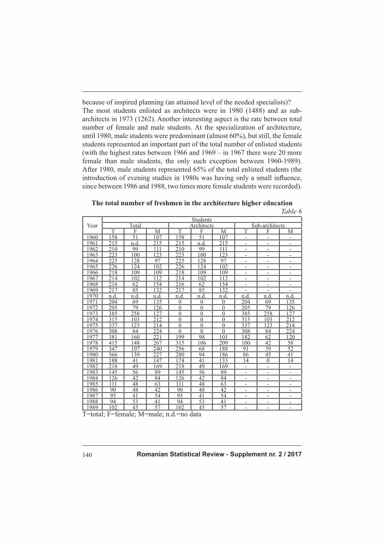
Romanian Statistical Review - Supplement nr. 2 / 2017140

because of inspired planning (an attained level of the needed specialists)? The most students enlisted as architects were in 1980 (1488) and as sub-architects in 1973 (1262). Another interesting aspect is the rate between total number of female and male students. At the specialization of architecture, until 1980, male students were predominant (almost 60%), but still, the female students represented an important part of the total number of enlisted students (with the highest rates between 1966 and 1969 – in 1967 there were 20 more female than male students, the only such exception between 1960-1989). After 1980, male students represented 65% of the total enlisted students (the introduction of evening studies in 1980s was having only a small infl uence, since between 1986 and 1988, two times more female students were recorded).

The total number of freshmen in the architecture higher education

Table 6

YearStudents

Total Architects Sub-architectsT F M T F M T F M

1960 158 51 107 158 51 107 - - -1961 215 n.d. 215 215 n.d. 215 - - -1962 210 99 111 210 99 111 - - -1963 223 100 123 223 100 123 - - -1964 225 128 97 225 128 97 - - -1965 226 124 102 226 124 102 - - -1966 218 109 109 218 109 109 - - -1967 214 102 112 214 102 112 - - -1968 216 62 154 216 62 154 - - -1969 217 85 132 217 85 132 - - -1970 n.d. n.d. n.d. n.d. n.d. n.d. n.d. n.d. n.d.1971 204 69 135 0 0 0 204 69 1351972 205 79 126 0 0 0 205 79 1261973 385 258 127 0 0 0 385 258 1271974 315 103 212 0 0 0 315 103 2121975 337 123 214 0 0 0 337 123 2141976 308 84 224 0 0 0 308 84 2241977 381 160 221 199 98 101 182 62 1201978 415 148 267 315 106 209 100 42 581979 347 107 240 256 68 188 91 39 521980 366 139 227 280 94 186 86 45 411981 188 41 147 174 41 133 14 0 141982 218 49 169 218 49 169 - - -1983 145 56 89 145 56 89 - - -1984 126 42 84 126 42 84 - - -1985 111 48 63 111 48 63 - - -1986 90 48 42 90 48 42 - - -1987 95 41 54 95 41 54 - - -1988 94 53 41 94 53 41 - - -1989 102 45 57 102 45 57 - - -

T=total; F=female; M=male; n.d.=no data

Revista Română de Statistică - Supliment nr. 2 / 2017 141

The statistical data from National Institute of Statistics reveals that between (at least) 1971 and 1976 there was no admission at the specialization architecture and systematization. As the only institution of higher education to host specialization for architects, “Ion Mincu” Institute of Architecture from Bucharest was not receiving freshmen. This is in contradiction with the information from Admiterea, a ”canon” publication for higher education. Here we fi nd that from 1971 to 1973 the admission was carried out only for

sub-architects specialists (architecture specialization) at institutions from

Bucharest, Iași, Cluj-Napoca and Timișoara (then for two and a half years of study, from 1971/1972, with 3 years [25]), and only from 1974 we fi nd

architects to be trained at Bucharest with a clear mention:

,,The admission exam at sections of architecture (sub-architects) is

organized at the “Ion Mincu” Institute of Architecture from Bucharest and at

polytechnics institutes from Cluj, Iași and Timișoara. At the architecture and systematization section (second level of education-architects) are admitted at “Ion Mincu” only graduates of the third year, with diploma exam from all architecture sections, in the limit of study places plans for the second level of education” [26]. In this case, the fi rst sub-architects graduates of 1973 could have

entered the second level of education, for becoming architects, in 1974, but

no one could have study to become architect between 1971 and 1973, as “Ion

Mincu” Institute did not support this type of education in that period and even

less the other centres, which were never entitled to do so. This means that in

the mentioned period, all students were bound to graduate as sub-architects

and, in a cynical way, we can say the communist regime ensured that a

measure taken in the human capital planning was having the expected results,

thus leaving any other discussions about the freedom of education to be self-

explanatory and reasons to introduce sub-architects education, like ensuring a

spirit of social justice, fostering the training of students, selection of the most

valuable students and rational use of material and didactic potential [27], just

to be “sprayed” by propaganda.

Another measure taken with care for the planning, not for the people

was from 1977, when those studying to become sub-architects could not

continue their studies in order to become architects [28], This time at least

everybody knew it (how soon this measure was public?).

The measures taken to ensure the training of sub-architects reveals two

forms of short term education: enclosed – without the possibility to continue

the studies (typical for sub-engineers) and open – with possibility to continue

studies to graduate as “full-status specialist” (typical for dentists specialists).

Thanks to statistics, when looking at disaggregated data for the

freshmen at the architecture and systematization specialization since 1979, we

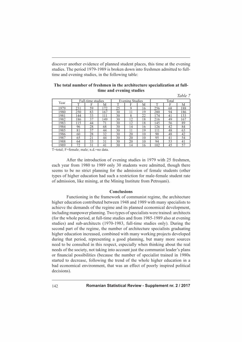
Romanian Statistical Review - Supplement nr. 2 / 2017142

discover another evidence of planned student places, this time at the evening studies. The period 1979-1989 is broken down into freshmen admitted to full-time and evening studies, in the following table:

The total number of freshmen in the architecture specialization at full-

time and evening studies

Table 7

Year Full-time studies Evening Studies TotalT F M T F M T F M

1979 231 59 172 25 9 16 256 68 1881980 250 83 167 30 11 19 280 94 1861981 144 33 111 30 8 22 174 41 1331982 186 37 149 30 12 18 216 49 1671983 115 44 71 30 12 18 145 56 891984 96 28 68 30 14 16 126 42 841985 81 37 44 30 11 19 111 48 631986 60 28 32 30 20 10 90 48 421987 65 21 44 30 20 10 95 41 541988 64 33 31 30 20 10 94 53 411989 72 31 41 30 14 16 102 45 57

T=total; F=female; male; n.d.=no data.

After the introduction of evening studies in 1979 with 25 freshmen, each year from 1980 to 1989 only 30 students were admitted, though there seems to be no strict planning for the admission of female students (other types of higher education had such a restriction for male-female student rate of admission, like mining, at the Mining Institute from Petroșani).

Conclusions

Functioning in the framework of communist regime, the architecture higher education contributed between 1948 and 1989 with many specialists to achieve the demands of the regime and its planned economical development, including manpower planning. Two types of specialists were trained: architects (for the whole period, at full-time studies and from 1985-1989 also at evening studies) and sub-architects (1970-1983, full-time studies only). During the second part of the regime, the number of architecture specialists graduating higher education increased, combined with many working projects developed during that period, representing a good planning, but many more sources need to be consulted in this respect, especially when thinking about the real needs of the society, not taking into account just the communist leader’s plans or fi nancial possibilities (because the number of specialist trained in 1980s started to decrease, following the trend of the whole higher education in a bad economical environment, that was an effect of poorly inspired political decisions).

Revista Română de Statistică - Supliment nr. 2 / 2017 143

The most important period of accumulation of human capital was during 1970s (in average 390 graduates), when architects and sub-architects graduated from the institutions of architecture higher education: “Ion Mincu” Institute of Architecture from Bucharest was the most important such institution (with architecture and systematization specialization – training of architects and architecture specialization – training of sub-architects in short term education, 3 instead of 6 years of studies), but other three institution contributed through their sections of architecture (polytechnics institutes from Iași, Cluj-Napoca and Timișoara). They all trained over 7000 architects and sub-architects. We have analyzed and verifi ed from many sources different sets of data revealing interesting aspects of the accumulation of human capital, but also we have identifi ed some of the most important characteristics of the type of specialists trained (status of the graduates, constraints in training), and milestones of the architecture higher education, with the help of statistical data and other sources.

Acknowledgment

This work was supported by a grant of the Romanian National Authority for Scientifi c Research, CNCS –UEFISCDI, project number PN-II-ID-PCE-2011-3-0476.

Endnotes

[1] Decretul nr. 175 din 3 august 1948 pentru reforma învățământului, Colecţiune de legi, decrete şi deciziuni, august 1948, p. 1676-1682. [2] Deciziunea nr. 253.499 din 26 octombrie 1948 privind organizarea învățământului superior, Colecţiune de legi, decrete şi deciziuni, octombrie 1948, p 952-963; from 14 November 1952 the Institute of Architecture, took the name “Ion Mincu” after Decree 147/1953 (https://www.uauim.ro/universitatea/istoric/). [3] Paramount for the organization of higher education are: ***, Admiterea în învățămîntul superior 1968-1981; ,,Forum”, 1982-1989. [4] Hotărârea nr. 372 din 8 aprilie 1972 privind subordonarea unor instituții de învățămînt superior, Colecţia de Hotărîri ale Consiliului de Miniştri și alte acte normative,

aprilie-iunie 1972, p. 16-24.

[5] Ioan Silviu Nistor, Istoria învățământului tehnic din Cluj-Napoca, ed. a 2-a, Cluj-

Napoca, Editura U.T Pres, 2004, p. 220.

[6] From the many proposals arising, it was even considered the measure of

establishing a new institution of higher education for architecture in Cluj-Napoca, The Institute

for Construction and Architecture, with faculties of construction and architecture and urbanism

(Ioan Silviu Nistor, Istoria învățământului tehnic din Cluj-Napoca, ed. a 2-a, Cluj-Napoca,

Editura U.T Pres, 2004, p. 220-222, 238-246).

[7] Bogdan Murgescu, Andrei Florin Sora, Dynamics of Qualifi cations in Romanian

Higher Education (1968-2010), ,,Manager Journal”, 2013, no. 18, p. 30-39; Andrei Florin Sora,

Evoluția califi cărilor din învățământul universitare românesc 1968-2011, 2011. Available from:

http://www.invatamant-superior.ro/wp-content/uploads/2013/08/Raport_istoria_califi carilor.pdf.

Romanian Statistical Review - Supplement nr. 2 / 2017144

[8] Ordinul Ministerului Învățământului nr. 856 din 31 iulie 1970. [9] Jan Sadlak, Planning of Higher Education in Countries with a Centrally Planned Socio-economic System: Case Study of Poland and Romania, State University of New York Buffalo, 1988, p. 345. [10] The training of dentists was called an experiment (C. Gh. Marinescu, Un secol de învățămînt medical superior la Iași. Institutul de Medicină și Farmacie (1948-1979), Iași, 1979, p. 37; C. Anastasatu, Învățămîntul superior de scurtă durată în medicină și farmacie, în „Forum”, nr. 2 din 1974, p. 16, 17) and maybe in the future we will have a study about them. [11] Decretul Consiliului de Stat (DCS) nr. 147 din 5 iunie 1974 privind nomenclatorul profi lelor și specializărilor din învățământul superior, precum și instituțiile și facultățile din sistemul Ministerului Educației și Învățământului; DCS nr. 209 din 12 iulie 1977 pentru modifi carea anexelor nr. 1 și 2 la DCS nr. 147/1974. [12] Ascanio Damian, Învățământul superior de arhitectură într-o nouă viziune organizatorică, în „Forum”, nr. 8 din 1970, p. 9. [13] See also the important aspects highlighted by Ioan Silviu Nistor, Istoria

învățământului tehnic din Cluj-Napoca, ed. a 2-a, Cluj-Napoca, Editura U.T Pres, 2004, p. 217. [14] Mariana Nicolescu, Absolvenții – o forță de muncă insufi cient folosită, în „Forum”, nr. 7 din 1977, p. 61. [15] Legea nr. 11 din 13 mai 1968 (Legea privind învățămîntul în Republica Socialistă România), în Colecţie de legi, decrete, hotărîri şi alte acte normative, martie-aprilie 1968, p. 61. [16] Legea nr. 28 din 26 decembrie 1978 (Legea Educației și Învățămîntului), în ,,Buletinul Ofi cial al Republicii Socialiste România”, nr. 113 din 26 decembrie 1978. [17] Legea nr. 12 din 21 octombrie 1971 privind încadrarea și promovarea în muncă a personalului din unitățile socialiste de stat, consultabilă la adresa http://lege5.ro. [18] Legea nr. 57 din 29 octombrie 1974 (Legea retribuirii după cantitatea și calitatea muncii), în Colecția de legi și decrete, iulie-septembrie 1980, p. 25, 118, 175, 176. [19] ***, Admiterea în învățămîntul superior 1979, p. 50. [20] Please consult the reference for all the documents used. [21] ***, Învățământul în România – date statistice, 1994; ***, Învățământul în România – date statistice, 1996. [22] Secția Arhivele Naționale Istorice Centrale, fond CC al PCR - Secția Economică, dosar nr. 57/1987, f. 8-10. [23] Hotărârea Plenarei CC al PCR din 18-19 iunie 1973 cu privire la dezvoltarea și perfecționarea învățământului în Republica Socialistă România. [24] Bogdan Murgescu, România și Europa. Acumularea decalajelor economice (1500-2010), Iași, Editura Polirom, 2010, p. 392-407. [25] Hotărârea nr. 1245 din 7 octombrie 1971 privind durata studiilor la învățămîntul de subingineri, în Colecţia de Hotărîri ale Consiliului de Miniştri și alte acte normative, octombrie-decembrie 1971, p. 18. [26] ***, Admiterea în învățămîntul superior 1974, p. 13. [27] Ioan Hedeșiu, Probleme ale dezvoltării învățământului superior de scurtă durată, în „Forum”, nr. 2 din 1974, p. 11. [28] Ioan Silviu Nistor, Istoria învățământului tehnic din Cluj-Napoca, ed. a 2-a, Cluj-Napoca, Editura U.T Pres, 2004, p. 222.

Revista Română de Statistică - Supliment nr. 2 / 2017 145

References

1. Marinescu, C. Gh. 1979, Un secol de învățămînt medical superior la Iași. Institutul de Medicină și Farmacie (1948-1979), Editura IMF, Iași.

2. Murgescu, B. 2010, România și Europa. Acumularea decalajelor economice (1500-2010), Editura Polirom, Iași.

3. Nistor, I. S. 2004, Istoria învățământului tehnic din Cluj-Napoca, Editura U.T Pres, Cluj-Napoca.

4. Sadlak, J. 1988, Planning of Higher Education in Countries with a Centrally Planned Socio-economic System: Case Study of Poland and Romania, State University of New York Buffalo.

5. Sora, A. F. 2011, Evoluția califi cărilor din învățământul universitare românesc 1968-2011, freely available at http://www.invatamant-superior.ro/wp-content/uploads/2013/08/Raport_istoria_califi carilor.pdf, 18-08-2016.

6. Anastasatu, C. 1974, “Învățămîntul superior de scurtă durată în medicină și farmacie”, Forum, 2, 16-17.

7. Damian, A. 1970, ”Învățământul superior de arhitectură într-o nouă viziune organizatorică”, Forum, 8, 7-10.

8. Hedeșiu, I. 1974, “Probleme ale dezvoltării învățământului superior de scurtă durată”, Forum, 2, 6-16.

9. Murgescu, B., Sora, A. F. 2013, “Dynamics of Qualifi cations in Romanian Higher Education (1968-2010)”, Manager Journal, 18, 30-39.

10. Nicolescu, M. 1977, “Absolvenții – o forță de muncă insufi cient folosită”, Forum, 7, 61-64.

11. Decretul Consiliului de Stat (DCS) nr. 147 din 5 iunie 1974 privind nomenclatorul profi lelor și specializărilor din învățământul superior, precum și instituțiile și facultățile din sistemul Ministerului Educației și Învățământului.

12. DCS nr. 209 din 12 iulie 1977 pentru modifi carea anexelor nr. 1 și 2 la DCS nr. 147/1974.

13. Decretul nr. 175 din 3 august 1948 pentru reforma învățământului, Colecţiune de legi, decrete şi deciziuni, august 1948, p. 1676-1682.

14. Deciziunea nr. 253.499 din 26 octombrie 1948 privind organizarea învățământului superior, Colecţiune de legi, decrete şi deciziuni, octombrie 1948, p 952-963.

15. Hotărârea nr. 372 din 8 aprilie 1972 privind subordonarea unor instituții de învățămînt superior, Colecţia de Hotărîri ale Consiliului de Miniştri și alte acte normative, aprilie-iunie 1972, p. 16-24.

16. Ordinul Ministerului Învățământului nr. 856 din 31 iulie 1970. 17. Hotărârea Plenarei CC al PCR din 18-19 iunie 1973 cu privire la dezvoltarea și

perfecționarea învățământului în Republica Socialistă România. 18. Hotărârea nr. 1245 din 7 octombrie 1971 privind durata studiilor la învățămîntul de

subingineri, Colecţia de Hotărîri ale Consiliului de Miniştri și alte acte normative, octombrie-decembrie 1971.

19. Legea nr. 12 din 21 octombrie 1971 privind încadrarea și promovarea în muncă a personalului din unitățile socialiste de stat, consultabilă la adresa http://lege5.ro.

20. Legea nr. 57 din 29 octombrie 1974 (Legea retribuirii după cantitatea și calitatea muncii), Colecția de legi și decrete, iulie-septembrie 1980.

21. Legea nr. 11 din 13 mai 1968 (Legea privind învățămîntul în Republica Socialistă România), Colecţie de legi, decrete, hotărîri şi alte acte normative, martie-aprilie 1968.

Romanian Statistical Review - Supplement nr. 2 / 2017146

22. Legea nr. 28 din 26 decembrie 1979 (Legea Educației și Învățămîntului), ,,Buletinul Ofi cial al Republicii Socialiste România”, nr. 113 din 26 decembrie 1978.

23. Arhiva Institutului Național de Statistică, Analiza învățămîntului superior la începutul anului școlar 1954/55 – cursuri de zi.

24. Arhiva Institutului Național de Statistică, Situația elevilor și studenților la începutul anului școlar 1955/56.

25. Arhiva Institutului Național de Statistică, Situația elevilor și studenților la începutul anului școlar 1956/57 (analiza).

26. Arhiva Institutului Național de Statistică, Situația învățămîntului superior la începutul anului școlar 1957/58 – cursuri de zi.

27. Arhiva Institutului Național de Statistică, Situația învățămîntului superior la începutul anului școlar 1959-1960 – cursuri de zi.

28. Arhiva Institutului Național de Statistică, Situația învățămîntului superior (inclusiv institutele pedagogice de profesori de 3 ani) la începutul anului universitar 1960/1961 – cursuri de zi.

29. Arhiva Institutului Național de Statistică, Situația învățămîntului superior la începutul anului universitar 1961/1962 – învățămînt de zi.

30. Arhiva Institutului Național de Statistică, Situația învățămîntului superior la începutul anului universitar 1962/1963 – învățămînt de zi.

31. Arhiva Institutului Național de Statistică, Situația învățămîntului superior la începutul anului universitar 1963/1964 – 1969/1970 (annual publication).

32. Arhiva Institutului Național de Statistică, Numărul studenților și cadrelor didactice din instituțiile de învățămîntului superior la începutul anului universitar 1971/1972.

33. Arhiva Institutului Național de Statistică, Învățămîntul superior la începutul anului universitar 1972/1973 – 1988-1989 (annual publication).

34. Arhiva Institutului Național de Statistică, Desvoltarea învățământul în perioada 1938-1951.

35. Arhiva Institutului Național de Statistică, Situația învățămîntului de toate gradele în anii școlari 1938/39, 1948/49, 1950/51-1956/57 pe regiuni.

36. Arhiva Institutului Național de Statistică, Analiza de sfârșit de an școlar 1951/52 iulie.

37. Arhiva Institutului Național de Statistică, Analiza de sfârșit de an școlar 1952-53 în învățământul superior.

38. Arhiva Institutului Național de Statistică, Analiza de sfârșit de an școlar 1953-54 sept.-octombrie. Învățămînt superior.

39. Arhiva Institutului Național de Statistică, Situația la învățătură a elevilor și studenților la sfîrșitul anului școlar 1954/55-1959/60 (annual publication).

40. Arhiva Institutului Național de Statistică, Repartizarea studenților după situația la învățătură la sfîrșitul anului universitar 1960/1961 – sesiunea septembrie – învățământ de zi și seral.

41. Arhiva Institutului Național de Statistică, Situația la învățătură a studenților la sfîrșitul anului universitar 1961/1962 – sesiunea septembrie – învățămînt de zi.

42. Arhiva Institutului Național de Statistică, Situația studenților la sfîrșitul anului universitar 1962/1963-1968/1969 (annual publication).

Revista Română de Statistică - Supliment nr. 2 / 2017 147

43. Arhiva Institutului Național de Statistică, Rezultatele la învățătură ale studenților

la sfîrșitul anului universitar 1969-1970 – învățămînt de zi și seral. 44. Arhiva Institutului Național de Statistică, Rezultatele la învățătură ale studenților

la sfîrșitul anului universitar 1970-1971. 45. Arhiva Institutului Național de Statistică, Situația la învățătură a studenților la

sfîrșitul anului universitar 1971/1972 – 1978/1979 (annual publication). 46. Arhiva Institutului Național de Statistică, Învățămîntul superior la sfîrșitul anului

universitar 1979/1980-1988/1989 (annual publication). 47. Secția Arhivele Naționale Istorice Centrale, fond CC al PCR - Secția Propagandă și

Agitație, dosar nr. 117/1989 (Învățămîntul superior la începutul anului universitar 1989-1990, 1989).

48. Secția Arhivele Naționale Istorice Centrale, fond CC al PCR - Secția Economică, dosar nr. 57/1987.

49. ***, Populația Republicii Populare Române a 25 ianuarie 1948, extras din ,,Probleme economice”, nr. 2, martie 1948.

50. ***, Recensămîntul populației și al locuințelor din 21 februarie 1956, Direcția Centrală de Statistică, 1959.

51. ***, Recensămîntul populației și al locuințelor din 15 martie 1966, vol I, Direcția Centrală de Statistică, 1969.

52. ***, Recensămîntul populației și al locuințelor din 5 ianuarie 1977, vol I, II, Direcția Centrală de Statistică, 1980.

53. ***, Recensământul populației și al locuințelor din 7 ianuarie 1992, vol I, II, Direcția Centrală de Statistică, 1994.

54. ***, Învățământul în România – date statistice, 1994. 55. ***, Învățământul în România – date statistice, 1996. 56. ***, Admiterea în învățămîntul superior 1968-1981 (annual publication). 57. Forum, 1982-1989 (annual publication).

Romanian Statistical Review - Supplement nr. 2 / 2017148

Methodological and Applicative Problems of using Pearson Correlation Coeffi cient in the

Analysis of Socio-Economic Variables

Daniela-Emanuela Dănăcică

Faculty of Economics, Constantin Brâncuși University of Târgu-Jiu

Abstract

The aim of this paper is to focus on the methodological and applicative

problems that Pearson correlation coeffi cient may arise when used to

analyzing the relationship between socio-economic variables. Using real data

we empasized the effect of the most important factors infl uencing the size and

interpretation of Pearson coeffi cient and we presented the special cases of this

statistics and their usefulness.

Keywords: correlation, Pearson coeffi cient, size, linearity

JEL Classifi cation: C18, C01

1. Introduction

If we focus on the name of simple linear correlation coeffi cient,

known in the literature as “Pearson product-moment correlation coeffi cient”,

we could erroneously belive that the English mathematician and biostatistician

Karl Pearson developed this coeffi cient himself. In fact, it was Francis Galton

the man who fi rst conceived and formulated the concepts of correlation

and regression (Stanton, 2001). Later on, Bravais and Pearson elaborated a

rigourous mathematical approach for correlation and regression.

Pearson product-moment correlation coeffi cient is widely used in

economics, social sciences, medicine, etc., as a measure of linear relationship

between two variable X and Y. The mathematical formula for this coeffi cient

developed by Pearson in 1895 is:

� �

�

� �

�

��

��

��

�

�

�

��

�

�

�

�

��

����

����

' '

>'

'>

?;9;9@

;;99

���������������������������������������������������

�

�

(1)

Since :�� ���

����

���

�

�

� ;;99

;� ��9 '

��

��� ��/��+����, we have

���/��+����

��

���

��

��

;� ��9> � �������������������������������������������������9 (2)

Revista Română de Statistică - Supliment nr. 2 / 2017 149

therefore, as Rodgers and Nicewander (1988) underline, Pearson coeffi cient

can be described as a standardized covariance.

In statistics is widely used the following formula:

−

−

⋅−=

∑∑∑ ∑

∑∑ ∑

=== =

== =

n

i

i

n

i

i

n

i

n

i

ii

n

i

i

n

i

n

i

iii

xy

yynxxn

yxyxn

r

1

2

1

2

1 1

22

11 1/

)(

(3)

[ ]1,1/ −∈xyr . The closer the value of xyr / is to +1 or -1, the higher the

association between these two variables is; the closer the value of xyr / is to 0,

the weaker the strengh of the relationship is.

In many statistics textbooks the interval [-1, 1] is divided in subintervals;

the intensity of relationship between X and Y is interpreted depending on the

subintervals of which xyr / belongs. However, a specifi c value of Pearson

coeffi cient is difi cult to interpret. For example, it is diffi cult to interpret a

0.6 value of xyr / compared with a 0.7 value. Rinaman (1993) underlines that

there is no precise interpretation that could be attached to particular values of

Pearson correlation coeffi cient. Also, since ]1,0[/ ∈xyr there is a tendency

to mistakenly interpret its value as the proportion of identical ( ii yx , ) pairs, or

as the probability of a correct prediction (Falk and Well, 1997; Eisenbach and

Falk, 1984).

Although Pearson correlation is widely used by researchers from

many research areas and all the basic statistics textbooks cover the topic of

correlation, there are not so many studies focused on the subtle nuances of this

measure and on the atypical cases of Pearson coeffi cient and their usefulness.

Various analyzes about what is communicated using Pearson coeffi cient must

be carefully presented, because the similarities between some interpretation

are subject to specifi c constraints (Falk and Well, 1997). Each result obtained

using this statistics should be carefully checked if the intepretation is

appropriate to the used model; some interpretation of Pearson correlation

coeffi cient are valid only under certain particular circumstances.

The aim of this article is to emphasize the methodological and

applicative problems of using Pearson coeffi cient in the analysis of relationship

between socio-economic variables. Pearson coeffi cient is a versatile statistics

and it has many subtile shades. We will focus on the most important factors

affecting the value and interpretation of Pearson coeffi cient and on the

limitation of this statistics. We will discuss about particular cases when one or

both of the analyzed variables are dichotomous and we will present the special

Romanian Statistical Review - Supplement nr. 2 / 2017150

cases of Pearson coeffi cient and their particularities. To our knowledge, there

is no statistics textbooks in our country that cover aspects regarding factors

infl uencing the size and interpretation of Pearson coeffi cient, or aspects

regarding special cases of Pearson coeffi cient (other than Spearman and

Kendall coeffi cient). Thus this paper seeks to fi ll a gap in the existing literature

too.

2. Factors infl uencing the size and interpretation of Pearson correlation

coeffi cient

In this section of paper we will analyze the effect of main factors

infl uencing the size and interpretation of Pearson correlation coeffi cient.

The most important factors that have a signifi cant effect on the value and

interpretation of Pearson correlation coeffi cient are: the shape of distribution,

the size of sample, the aberrant values (outliers), the restriction of range and

nonlinearity, a third variable or more (Chen and Popovich, 2002; Goodwin

and Leech, 2006).

In every statistics textbooks it is written that Pearson correlation

coeffi cient has values within the [-1,1] interval. However, this is true only

if the distribution of exogenous X and endogenous Y are symmetrical and

has the same shape (Goodwin and Leech, 2006; Chen and Popovich, 2002;

Glass and Hopkins, 1996; Hays, 1994; Nunnally and Bernstein, 1994). If

the distribution of the analyzed variables does not share the same shape, the

increase of the exogenous X will not always be accompanied by the increase

of endogenous Y, in case of a positive relationship, or by the decrease of Y in

case of a negative relationship. According to Chen and Popovich (2002) and

Carrol (1961), the less similar the shape of distributions for both analyzed

variables, the smaller the maximum value of || / xyr will be. Goodwin and

Leech (2006) show that if the Pearson coeffi cient has the value xyr / =0,90

for two same-shaped distributions, changes in the form of one distribution

could decrease the value of Pearson coeffi cient from 0.80 to 0.70. However, if

we have a value of =xyr / 0,3 for two same-shaped distribution, even major

changes of the shape of one distribution will have a very low effect on the

estimated value of xyr / .

The size of sample for which Pearson correlation is estimated is

another important factor infl uencing its value and interpretation. The standard

error of xyr / is affected by the size of analyzed sample. According to Chen and

Popovich (2002), when the size of sample is equal with 20, approximately 95% of the correlation coeffi cients have their values in between [-0.47, 0.47]; when

the size of sample is of 102 empirical data, approximately 95% of coeffi cients

have values in between [-0.20, 0.20]. To emphasize the size effect on the

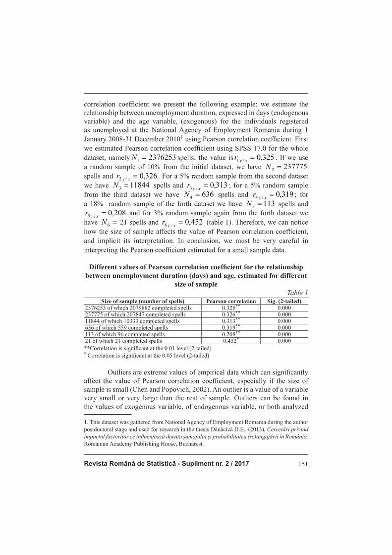
Revista Română de Statistică - Supliment nr. 2 / 2017 151

correlation coeffi cient we present the following example: we estimate the

relationship between unemployment duration, expressed in days (endogenous

variable) and the age variable, (exogenous) for the individuals registered

as unemployed at the National Agency of Employment Romania during 1

January 2008-31 December 20101 using Pearson correlation coeffi cient. First

we estimated Pearson correlation coeffi cient using SPSS 17.0 for the whole

dataset, namely 23762531 =N spells; the value is 325,0/1 =

xyr . If we use

a random sample of 10% from the initial dataset, we have 2377752 =N spells and 326,0/2 =

xyr . For a 5% random sample from the second dataset

we have 118443 =N spells and 313,0/3 =xy

r ; for a 5% random sample from the third dataset we have 6364 =N spells and 319,0/4 =

xyr ; for

a 18% random sample of the forth dataset we have 1135 =N spells and 208,0/5 =

xyr and for 3% random sample again from the forth dataset we have 216 =N 21 spells and 452,0/6 =

xyr (table 1). Therefore, we can notice

how the size of sample affects the value of Pearson correlation coeffi cient,

and implicit its interpretation. In conclusion, we must be very careful in

interpreting the Pearson coeffi cient estimated for a small sample data.

Different values of Pearson correlation coeffi cient for the relationship

between unemployment duration (days) and age, estimated for different

size of sample

Table 1Size of sample (number of spells) Pearson correlation Sig. (2-tailed)

2376253 of which 2079882 completed spells 0.325** 0.000237775 of which 207847 completed spells 0.326** 0.00011844 of which 10333 completed spells 0.313** 0.000636 of which 559 completed spells 0.319** 0.000113 of which 96 completed spells 0.208** 0.00021 of which 21 completed spells 0.452* 0.000**Correlation is signifi cant at the 0.01 level (2-tailed)* Correlation is signifi cant at the 0.05 level (2-tailed)

Outliers are extreme values of empirical data which can signifi cantly affect the value of Pearson correlation coeffi cient, especially if the size of sample is small (Chen and Popovich, 2002). An outlier is a value of a variable very small or very large than the rest of sample. Outliers can be found in the values of exogenous variable, of endogenous variable, or both analyzed

1. This dataset was gathered from National Agency of Employment Romania during the author postdoctoral stage and used for research in the thesis Dănăcică D.E., (2013), Cercetări privind

impactul factorilor ce infl uenţează durata șomajului şi probabilitatea (re)angajării în România,

Romanian Academy Publishing House, Bucharest.

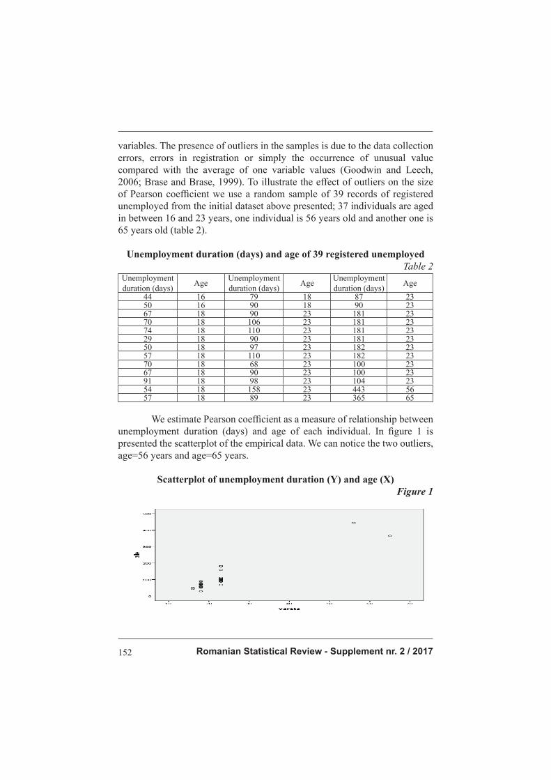
Romanian Statistical Review - Supplement nr. 2 / 2017152

variables. The presence of outliers in the samples is due to the data collection errors, errors in registration or simply the occurrence of unusual value compared with the average of one variable values (Goodwin and Leech, 2006; Brase and Brase, 1999). To illustrate the effect of outliers on the size of Pearson coeffi cient we use a random sample of 39 records of registered

unemployed from the initial dataset above presented; 37 individuals are aged

in between 16 and 23 years, one individual is 56 years old and another one is

65 years old (table 2).

Unemployment duration (days) and age of 39 registered unemployed

Table 2Unemployment

duration (days)Age

Unemployment

duration (days)Age

Unemployment

duration (days)Age

44 16 79 18 87 2350 16 90 18 90 2367 18 90 23 181 2370 18 106 23 181 2374 18 110 23 181 2329 18 90 23 181 2350 18 97 23 182 2357 18 110 23 182 2370 18 68 23 100 2367 18 90 23 100 2391 18 98 23 104 2354 18 158 23 443 5657 18 89 23 365 65

We estimate Pearson coeffi cient as a measure of relationship between

unemployment duration (days) and age of each individual. In fi gure 1 is

presented the scatterplot of the empirical data. We can notice the two outliers,

age=56 years and age=65 years.

Scatterplot of unemployment duration (Y) and age (X)

Figure 1

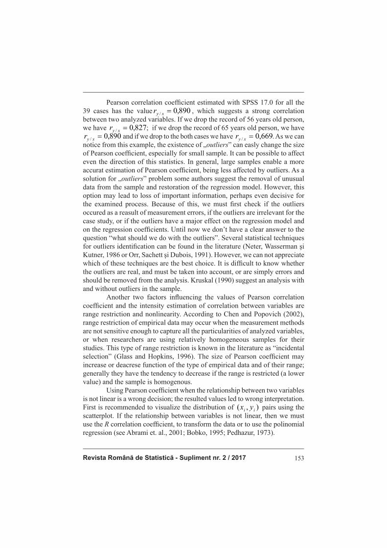
Revista Română de Statistică - Supliment nr. 2 / 2017 153

Pearson correlation coeffi cient estimated with SPSS 17.0 for all the

39 cases has the value 890,0/ =xyr , which suggests a strong correlation

between two analyzed variables. If we drop the record of 56 years old person,

we have 827,0/ =xyr ; if we drop the record of 65 years old person, we have

890,0/ =xyr and if we drop to the both cases we have 669,0/ =xyr . As we can

notice from this example, the existence of „outliers” can easly change the size

of Pearson coeffi cient, especially for small sample. It can be possible to affect

even the direction of this statistics. In general, large samples enable a more

accurat estimation of Pearson coeffi cient, being less affected by outliers. As a

solution for „outliers” problem some authors suggest the removal of unusual

data from the sample and restoration of the regression model. However, this

option may lead to loss of important information, perhaps even decisive for

the examined process. Because of this, we must fi rst check if the outliers

occured as a reasult of measurement errors, if the outliers are irrelevant for the

case study, or if the outliers have a major effect on the regression model and

on the regression coeffi cients. Until now we don’t have a clear answer to the

question “what should we do with the outliers”. Several statistical techniques

for outliers identifi cation can be found in the literature (Neter, Wasserman şi

Kutner, 1986 or Orr, Sachett şi Dubois, 1991). However, we can not appreciate

which of these techniques are the best choice. It is diffi cult to know whether

the outliers are real, and must be taken into account, or are simply errors and

should be removed from the analysis. Kruskal (1990) suggest an analysis with

and without outliers in the sample.

Another two factors infl uencing the values of Pearson correlation coeffi cient and the intensity estimation of correlation between variables are

range restriction and nonlinearity. According to Chen and Popovich (2002),

range restriction of empirical data may occur when the measurement methods

are not sensitive enough to capture all the particularities of analyzed variables,

or when researchers are using relatively homogeneous samples for their

studies. This type of range restriction is known in the literature as “incidental

selection” (Glass and Hopkins, 1996). The size of Pearson coeffi cient may

increase or deacrese function of the type of empirical data and of their range;

generally they have the tendency to decrease if the range is restricted (a lower

value) and the sample is homogenous.

Using Pearson coeffi cient when the relationship between two variables

is not linear is a wrong decision; the resulted values led to wrong interpretation.

First is recommended to visualize the distribution of ),( ii yx pairs using the

scatterplot. If the relationship between variables is not linear, then we must

use the R correlation coeffi cient, to transform the data or to use the polinomial

regression (see Abrami et. al., 2001; Bobko, 1995; Pedhazur, 1973).

Romanian Statistical Review - Supplement nr. 2 / 2017154

Sometimes two variables are statistically correlated, but in reality there is no causal relationship between them. In the literature this relationship is called „spourious correlation” or „illusory correlation”. „Spuorious correlation” was in attention of well-known statisticians like Yule, Hans Zeisel, Kendall or Lazarfeld. The occurence of spourious correlation may be the result of the effect of one or more so-called „a third variable”. For example we can fi nd mentioned in the literature the positive relationship between

age and job satisfaction of a person. Studies show that people satisfi ed with

their job within a company stay a longer time in their company. However,

the positive link between the two variables above mentioned may occur due

to the infl uence of a third variable, namely job tenure (Chen and Popovich,

2002). Another example widely presented in the literature is the one refered

to the link between religion and the height of European population. If we

move from northern Europe to the south, the proportion of Roman Catholic

population increases, while there is a decrease in the average height of the

inhabitants. The empirical data may suggest a negative correlation between

the Roman Catholic population and the height of individuals that belong to

this population. In reality this relationship is an illusory one, the height of

population depending on entirely other factors. The conclusion is that the

association does not alway imply causation between variables. A carefull

statistician should always keep that in mind.

3. Special cases of Pearson correlation coeffi cient xyr /

In this section of paper we will focus on special cases of Pearson

correlation coeffi cients, namely the point-bisearial correlation coeffi cient, phi

coeffi cient, biserial coeffi cient, tetrachoric coeffi cient and eta coeffi cient.

Point-biserial coeffi cient (

����� �������)����� ����� ����#��

�� �������������� ��9 �� ;�������,� ���� �������.������� ����������� ����� �

�����������+����,����+��)��� �������)��+�����������

) is a special case of Pearson correlation

coeffi cient, used to assess the type, the direction and the intensity of a

relationship between a countinous variable and a true dichotomous one. An

interesting fact is that the inference of point-biserial coeffi cient

����� �������)����� ����� ����#��

�� �������������� ��9 �� ;�������,� ���� �������.������� ����������� ����� �

�����������+����,����+��)��� �������)��+�����������

gives the

same information as an independent two sample t test, even they have different

focus (Chen and Popovich, 2002).

In the following, using the point-biserial coeffi cient we will analyze

the potential differences between male and female students regarding

the given importance to study of a second foreign language during their

undergraduate studies; we use a sample of 30 students from the second and

third year undergraduate program from Faculty of Economics, Constantin

Brâncuși University of Târgu-Jiu, Romania. The score given by students is the endogenous variable (Y) and the gender is the exogenous one (X). We will highlight the link between the two sample t test and the point biserial

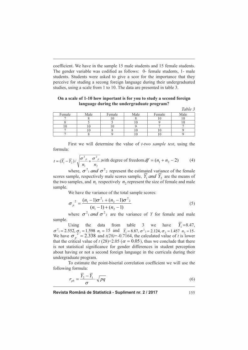
Revista Română de Statistică - Supliment nr. 2 / 2017 155

coeffi cient. We have in the sample 15 male students and 15 female students.

The gender variable was codifi ed as follows: 0- female students, 1- male

students. Students were asked to give a scor for the importance that they

perceive for studing a secong foreign language during their undergraduated

studies, using a scale from 1 to 10. The data are presented in table 3.

On a scale of 1-10 how inportant is for you to study a second foreign

language during the undergraduate program?

Table 3Female Male Female Male Female Male

7 8 10 8 10 108 5 5 10 9 10

10 10 10 9 7 77 10 8 10 10 97 8 9 10 10 9

First we will determine the value of t-two sample test, using the

formula:

2

2

1

2

21 /)(nn

YYtpp σσ

+−= ,with degree of freedom /��+�)�������������)�� ; 9 ' ��� ���� ��������������������������������������9!;���

�

�

�

%'(#'

�

(4)

where, 22

12 σσ and represent the estimated variance of the female

scores sample, respectively male scores sample, 21 YandY are the means of

the two samples, and 1n respectively 2n represent the size of female and male

sample.

We have the variance of the total sample scores:

)1()1(

)1()1(

21

22

212

12

−+−

−+−=

nn

nnp

σσσ (5)

where 22

12 σσ and are the variance of Y for female and male

sample.

Using the data from table 3 we have 81 =Y 8.47,

15598.1,552.2 1112 === nσσ 15 and '%!%F#'�' !# �2F#2

���� �� �� #�

�

%'(#'

�

.

We have 338.22 =pσ and t(28)=-0.7164, the calculated value of t is lower

that the critical value of t (28)=2.05 (� 9 2;K #$%�9 $%#$�� ;����� ���������)����,�� �,������-����+���������

�

�

%'(#'

�

), thus we conclude that there

is not statistical signifi cance for gender differences in student perception

about having or not a second foreign language in the curricula during their

undergraduate program.

To estimate the point-biserial correlation coeffi cient we will use the

following formula:

�-

���� �

��

�' ��������������������������������������������������� (6)

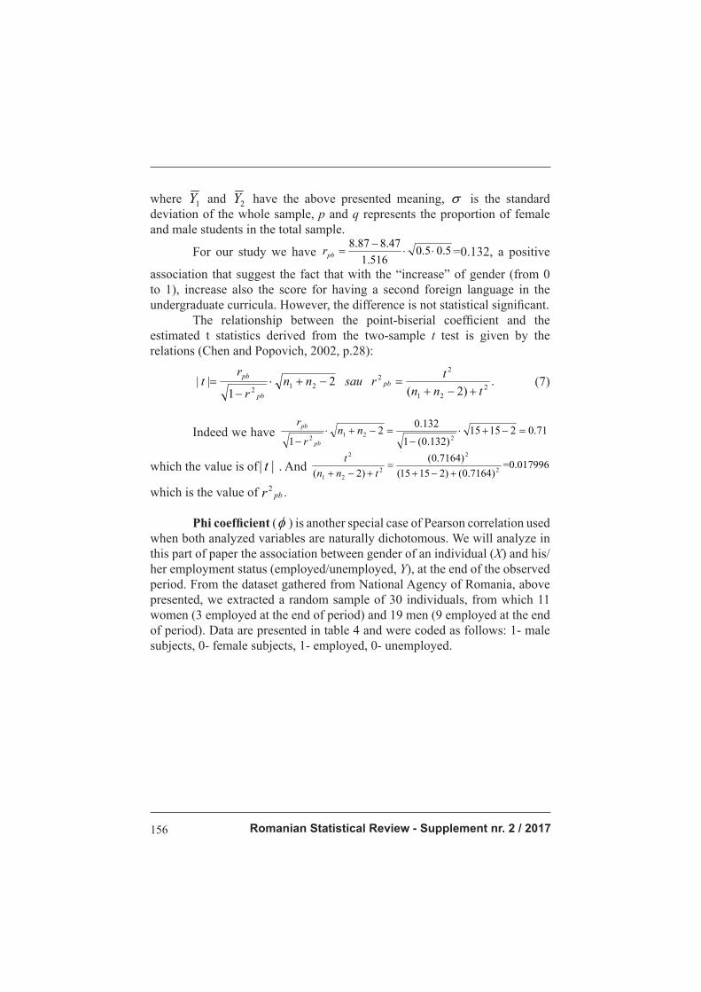
Romanian Statistical Review - Supplement nr. 2 / 2017156

where 1Y and 2Y have the above presented meaning, σ is the standard deviation of the whole sample, p and q represents the proportion of female and male students in the total sample.

For our study we have �����������)��/��+������ %#$%#$%'(#'

!F#22F#2��

���� K$#'& ����,������������ ��������+������������+��

�� �� �+���/��+� �+��5�� �����6�������)���9����$����';�� �� ������������+��� ��������+���������� ��)�

=0.132, a positive

association that suggest the fact that with the “increase” of gender (from 0 to 1), increase also the score for having a second foreign language in the undergraduate curricula. However, the difference is not statistical signifi cant.

The relationship between the point-biserial coeffi cient and the

estimated t statistics derived from the two-sample t test is given by the

relations (Chen and Popovich, 2002, p.28):

#; 9

'

JJ

'

' ���

�'����

� ��

��

��

�������

�� ��������������������������������������������������� (7)

Indeed we have 3�)��)�/�� +���� F'#$ '%'%;'& #$9'

'& #$

' '

����

�����

���

��

��� /+� +� �+�� ������ ���

;F'(!#$9�

�

which the value is of || t . And �#�G�)�

'

;F'(!#$9; '%'%9

;F'(!#$9

; 9 ����

��� ���

�K$#$'F==(�/+� +�����+�����������

�

which is the value of K$#$'F==(�/+� +�����+����������� �� #�

�

.

Phi coeffi cient (φ ) is another special case of Pearson correlation used

when both analyzed variables are naturally dichotomous. We will analyze in

this part of paper the association between gender of an individual (X) and his/

her employment status (employed/unemployed, Y), at the end of the observed

period. From the dataset gathered from National Agency of Romania, above

presented, we extracted a random sample of 30 individuals, from which 11

women (3 employed at the end of period) and 19 men (9 employed at the end

of period). Data are presented in table 4 and were coded as follows: 1- male

subjects, 0- female subjects, 1- employed, 0- unemployed.

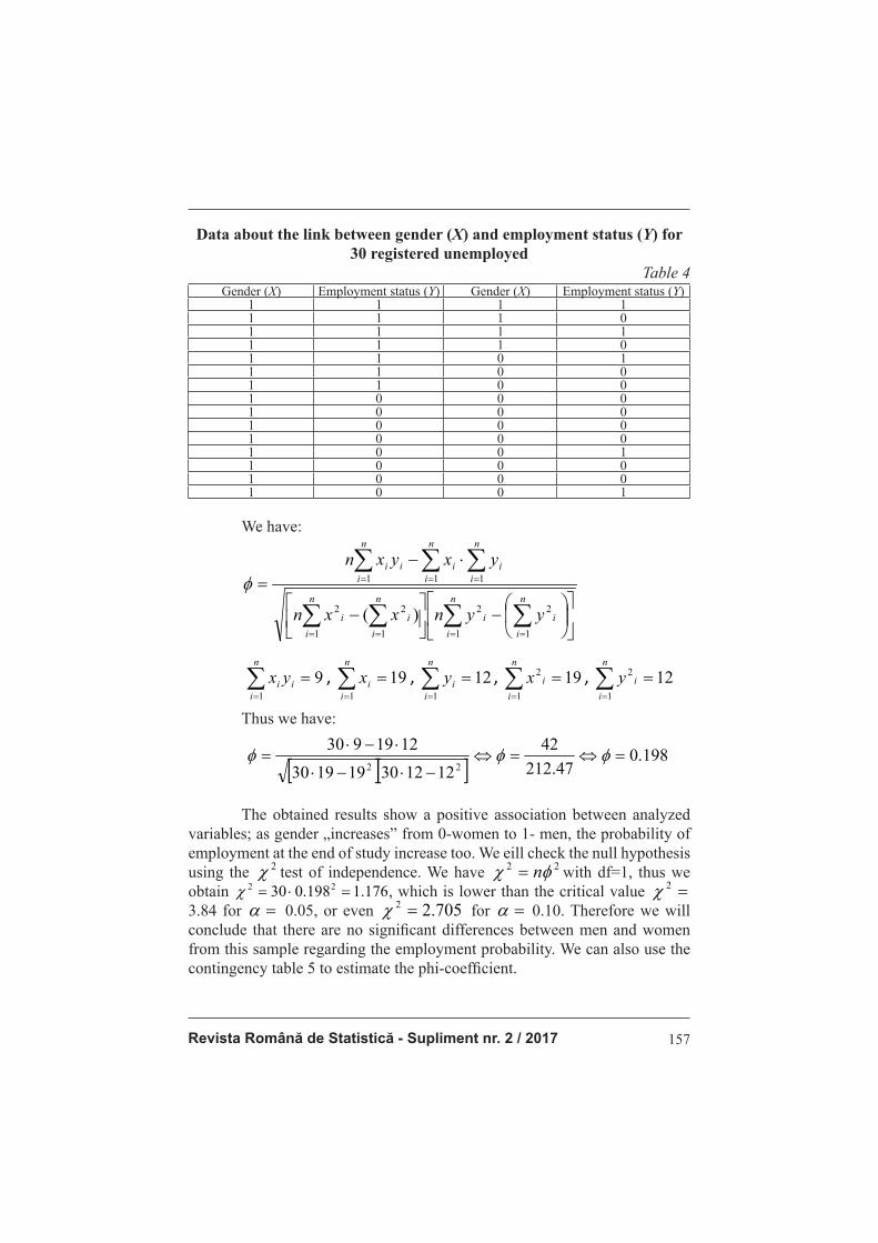
Revista Română de Statistică - Supliment nr. 2 / 2017 157

Data about the link between gender (X) and employment status (Y) for

30 registered unemployed

Table 4Gender (X) Employment status (Y) Gender (X) Employment status (Y)

1 1 1 11 1 1 01 1 1 11 1 1 01 1 0 11 1 0 01 1 0 01 0 0 01 0 0 01 0 0 01 0 0 01 0 0 11 0 0 01 0 0 01 0 0 1

We have:

−

−

⋅−=

∑∑∑ ∑

∑∑ ∑

=== =

== =

n

i

i

n

i

i

n

i

n

i

ii

n

i

i

n

i

n

i

iii

yynxxn

yxyxn

1

2

1

2

1 1

22

11 1

)(

φ

='

���

�

�

�

� �� �� '='

���

�

�

�� �� ' '

���

�

�

�� �� '='

���

�

�

�� �� ' '

���

�

�

�� �

� Thus we have:

�

� �� �'=2#$

!F# '

!

' ' &$'='=&$

' '==&$

����

����

���� ��� �

�

�� ��

� �

�

�����

�

�

The obtained results show a positive association between analyzed variables; as gender „increases” from 0-women to 1- men, the probability of employment at the end of study increase too. We eill check the null hypothesis using the 2χ test of independence. We have 22 φχ n= with df=1, thus we obtain )�K'���+���/���-����� 'F(#''=2#$&$ ���� ��/+� +������/����+����+�� ���� ��������� 2!

�� ��

�

��

�

, which is lower than the critical value 32 =χ 3.84 for .0=α 0.05, or even 705.22 =χ for 0=α 0.10. Therefore we will conclude that there are no signifi cant differences between men and women

from this sample regarding the employment probability. We can also use the

contingency table 5 to estimate the phi-coeffi cient.

Romanian Statistical Review - Supplement nr. 2 / 2017158

Contingency table for estimating phi coeffi cient

Table 5Unemployed (Y=0) Employed (Y=1) Total

Male (X=1) 10 a 9 b 19Female (X=0) 8 c 3 d 11Total 18 12 30

We estimate the phi correlation coeffi cient using the formula:

;;9;9;99 �� �� ��

���

����

��� �����

&$F �

, if ;

������ $;;9;9;99 ����� �� �� �� �����������������������������������������92;�

�

�

(8)

We have: H�� +���1� '=2#$;'2;9' ;9'';9'=9

&$F ��

�� �� � � ��)� �+�� �����,��������� ��� ������� ��� �+�� ���� and the interpretation

is similar to the one presented above.

Biserial correlation coeffi cient ( bisr ) is used when the exogenous

variable X has a normal distribution, but is artifi cially measured as a

dichotomous variable (e.g. accepted versus rejected, effi cient versus ineffi cient)

in its relationship with a continous endogenous Y variable (e.g. the results of an

admission exam, labor productivity of a sample of workers, etc). In oder words,

biserial coeffi cient is a statistic measure that allow us to estimate the strenght of

relationship between the exogenous X and the endogenous Y would be if X is not

artifi cially converted in a dichotomous variable (Chen and Popovich, 2002).

Biserial coeffi cient ( bisr ) has the following formula:

))(

(2

21

1212

nn

nnYYr

Y

bis +

−=

λσ (9)

where 2Y and 1Y are the mean of the two samples of endogenous

Y, 1n and 2n is the size of the samples and Yσ is the standard deviation of Y;

λ represents the ordinate of the standard normal distribution at )/( 212 nnn +proportion of subjects from the second sample.

The relationship between bisr and pbr is described by Chen and

Popovich (2002) as follows:

.)(

)1(3

21

2

2112

nn

nnnnrr pbbis +

−+=

λ (10)

Since .1)(

)1(3

21

2

2112 ≥+

−+

nn

nnnn

λ1.25, the value of biserial coeffi cient is

always higher than the value of point-biserial coeffi cient (Chen and Popovich,

2002, Glass and Hopkins, 1996).

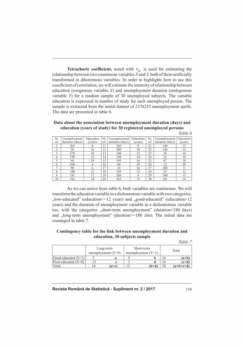
Revista Română de Statistică - Supliment nr. 2 / 2017 159

Tetrachoric coeffi cient, noted with tetr is used for estimating the relationship between two countinous variables X and Y, both of them artifi cially

transformed in dihotomous variables. In order to highlights how to use this

coeefi cient of correlation, we will estimate the intensity of relationship between

education (exogenous variable X) and unemployment duration (endogenous

variable Y) for a random sample of 30 unemployed subjects. The variable

education is expressed in number of study for each unemployed person. The

sample is extracted from the initial dataset of 2376253 unemployment spells.

The data are presented in table 6.

Data about the association between unemployment duration (days) and

education (years of study) for 30 registered unemployed persons

Table 6Nr. crt

Unemployment duration (days)

Education (years)

Nr.crt.

Unemployment duration (days)

Education (years)

Nr.crt

Unemployment duration (days)

Education (years)

1 365 8 11 260 8 21 140 132 20 16 12 300 10 22 156 123 270 10 13 240 12 23 30 164 190 12 14 190 14 24 32 165 60 18 15 195 16 25 67 186 360 4 16 40 18 26 12 207 90 6 17 10 16 27 300 98 180 12 18 185 12 28 23 129 181 12 19 360 4 29 180 13

10 182 14 20 365 12 30 181 14

As we can notice from table 6, both variables are continonus. We will

transform the education variable in a dichomotous variable with two categories,

„low-educated” (education<=12 years) and „good-educated” (education>12

years) and the duration of unemployment variable in a dichomotous variable

too, with the categories „short-term unemployment” (duration<180 days)

and „long-term unemployment” (duration>=180 zile). The initial data are

rearanged in table 7.

Contingency table for the link between unemployment duration and

education, 30 subjects sample

Table 7

Long-term

unemployment (Y=0)

Short-term

unemployment (Y=1)Total

Good-educated (X=1) 5 a 9 b 14 (a+b)Poor-educated (X=0) 13 c 3 d 16 (c+d)Total 18 (a+c) 12 (b+d) 30 (a+b+c+d)

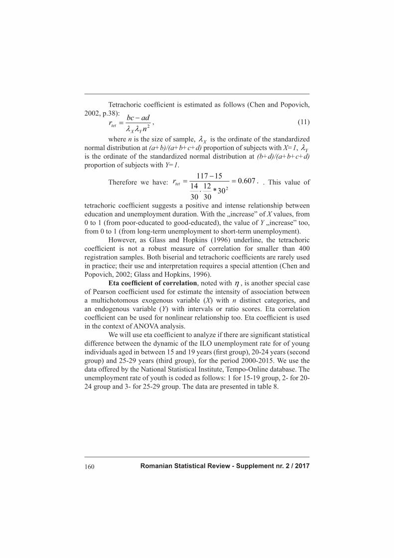
Romanian Statistical Review - Supplement nr. 2 / 2017160

Tetrachoric coeffi cient is estimated as follows (Chen and Popovich,

2002, p.38):

�

���

��

�����

�� ���������������������������������������������������, (11)

where n is the size of sample, Xλ is the ordinate of the standardized

normal distribution at (a+b)/(a+b+c+d) proportion of subjects with X=1, Yλis the ordinate of the standardized normal distribution at (b+d)/(a+b+c+d)

proportion of subjects with Y=1.

Therefore we have: �+�������� /�� +���1� ($F#$

&$N&$

'

&$

'!

'%''F

�

�

����� #� �+��� ������ ��� ����� +��� � ����� �����

�

S���� S���+�

���,������������

��)�� S���+�

���,������������

$$$� &#$$� '� '(#F$� �

$$'� $#2$� '� '%#=$� �

$$ � F#!$� '� '=#($� �

$$&� %#'$� '� '(#%$� �

$$!� =#$$� '� 'F#2$� �

$$%� %#$$� '� 'F#!$� �

$$(� =#'$� '� 'F#F$� �

$$F� F#!$� '� 'F#&$� �

$$2� 2#&$� '� '%#'$� �

$$=� &'#($� '� 'F#&$� �

$'$� F#'$� '� '#'$� �

$''� &$#F$� '� #%$� �

$' � &'#'$� '� $#2$� �

$'&� &'#%$� '� #'$� �

$'!� &!# $� '� '#2$� �

$'%� =#!$� '� '=#F$� �

. This value of

tetrachoric coeffi cient suggests a positive and intense relationship between

education and unemployment duration. With the „increase” of X values, from

0 to 1 (from poor-educated to good-educated), the value of Y „increase” too,

from 0 to 1 (from long-term unemployment to short-term unemployment).

However, as Glass and Hopkins (1996) underline, the tetrachoric

coeffi cient is not a robust measure of correlation for smaller than 400

registration samples. Both biserial and tetrachoric coeffi cients are rarely used

in practice; their use and interpretation requires a special attention (Chen and

Popovich, 2002; Glass and Hopkins, 1996).

Eta coeffi cient of correlation, noted with η , is another special case

of Pearson coeffi cient used for estimate the intensity of association between

a multichotomous exogenous variable (X) with n distinct categories, and

an endogenous variable (Y) with intervals or ratio scores. Eta correlation

coeffi cient can be used for nonlinear relationship too. Eta coeffi cient is used

in the context of ANOVA analysis.

We will use eta coeffi cient to analyze if there are signifi cant statistical

difference between the dynamic of the ILO unemployment rate for of young

individuals aged in between 15 and 19 years (fi rst group), 20-24 years (second

group) and 25-29 years (third group), for the period 2000-2015. We use the

data offered by the National Statistical Institute, Tempo-Online database. The

unemployment rate of youth is coded as follows: 1 for 15-19 group, 2- for 20-

24 group and 3- for 25-29 group. The data are presented in table 8.

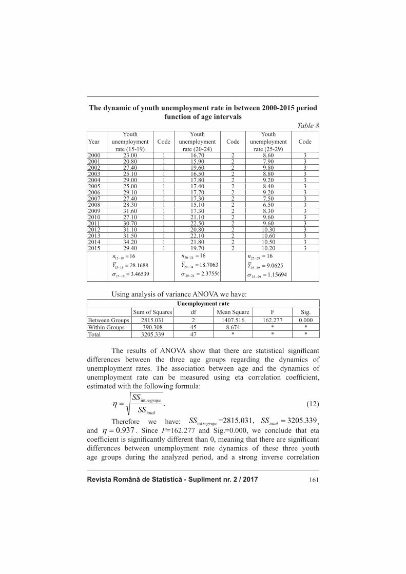
Revista Română de Statistică - Supliment nr. 2 / 2017 161

The dynamic of youth unemployment rate in between 2000-2015 period

function of age intervals

Table 8

YearYouth

unemployment rate (15-19)

CodeYouth

unemployment rate (20-24)

CodeYouth

unemployment rate (25-29)

Code

2000 23.00 1 16.70 2 8.60 32001 20.80 1 15.90 2 7.90 32002 27.40 1 19.60 2 9.80 32003 25.10 1 16.50 2 8.80 32004 29.00 1 17.80 2 9.20 32005 25.00 1 17.40 2 8.40 32006 29.10 1 17.70 2 9.20 32007 27.40 1 17.30 2 7.50 32008 28.30 1 15.10 2 6.50 32009 31.60 1 17.30 2 8.30 32010 27.10 1 21.10 2 9.60 32011 30.70 1 22.50 2 9.60 32012 31.10 1 20.80 2 10.30 32013 31.50 1 22.10 2 10.60 32014 34.20 1 21.80 2 10.50 32015 29.40 1 19.70 2 10.20 3�

&#!(%&=

2#'(22

'(

'='%

'='%

'='%

�

�

�

�

�

�

�

�

�

�

�

�

�

#&F%%(

'2#F$(&

'(

! $

! $

! $

�

�

�

�

�

�

�

�

��

�

�

#&F%%(

� �

'#'%(=!

=#$( %

'(

= %

= %

= %

�

�

�

�

�

�

�

�

�

��

�

Using analysis of variance ANOVA we have: Unemployment rate

Sum of Squares df Mean Square F Sig.Between Groups 2815.031 2 1407.516 162.277 0.000Within Groups 390.308 45 8.674 * *Total 3205.339 47 * * *

The results of ANOVA show that there are statistical signifi cant

differences between the three age groups regarding the dynamics of

unemployment rates. The association between age and the dynamics of

unemployment rate can be measured using eta correlation coeffi cient,

estimated with the following formula:

�������)�/��+��+�������/����������1�

#���

�����

�!���

&&

&&�� ��������������������������������������������������� (12)

Therefore we have: �+�������� /�� +���1� �!���&&��� K 2'%#$&'�� & $%#&&=������&& � ��)�

�

,

and 937.0=η . Since F=162.277 and Sig.=0.000, we conclude that eta

coeffi cient is signifi cantly different than 0, meaning that there are signifi cant

differences between unemployment rate dynamics of these three youth

age groups during the analyzed period, and a strong inverse correlation

Romanian Statistical Review - Supplement nr. 2 / 2017162

between age and unemployment rate of young people. If we use the mean values of unemployment rates instead of the codes 1, 2 and 3 (mean [15-19] unemployment rate= 28.1688 , mean [20-24] unemployment rate= 18.7063 and mean [25-34] unemployment rate=9.0625 ) and use the Pearson coeffi cient we get r= - 0,937, we observe that 937.0|| =r , which is exactly

the value of eta coeffi cient.

4. Conclusions

Pearson correlation coeffi cient is widely used in statistic analysis to

estimate the relationship between different variables; however its subtle nuances

and versatile nature are not generally well-known and are insuffi ciently investigated

in the literature. The aim of this paper was to analyze this complex measure and

to present its problems and limitations. We focused on the most important factors

infl uencing the size, direction and interpretation of Pearson coeffi cient; using real

data we proved that the interpretation of the values of Pearson coeffi cient must be

presented with caution. For each case we must check if the interpretation is in line

with the particularities of data and the used model. In all basic statistics textbooks

we can fi nd a chapter or a section devoted to simple linear correlation and Pearson

coeffi cient. However, only a few cover the topic of factors infl uencing the size

and interpretation of r (mostly the lack of linearity). To our knowledge, there is no

approach of these aspects in the Romanian basic statistics textbooks.

We focused also on particular cases when one or both of the analyzed

variables are naturally dichotomous or artifi cially converted as dichotomous

variable. Using real data we illustrated how to use the point-biserial coeffi cient,

phi coeffi cient, tetrachoric coeffi cient and eta coeffi cient and how to interpret

the obtained results. The issues presented in this paper can be useful to

researchers, tutors who teach statistics and students.

References

1. Abrami, P.C., Cholmsky, P., and Gordon, R. (2001), Statistical analysis for the

social sciences: An Interactive Approach. Needham Heights, MA: Allyn & Bacon. 2. Bobko, P. (1995), Correlation and Regression: Principles and Applications for

Industrial Organizational Psycology and Management, New York: Mc.Graw-Hill. 3. Brase, C.H. and Brase, C.P. (1999), Understanding statistics: Concepts and

Methods (6th ed.), Boston: Houghton Miffl in.

4. Cahan, S. (1965), On the Interpretation of the Product Moment Correlation

Coeffi cient as a Measure. Unpublished manuscript. The Hebrew University,

School of Education, Jerusalem, Israel.

4. Carroll, J. B. (1961), „The nature of the data, or how to choose a correlation

coeffi cient” Psychometrika, 26, pp. 247–272.

5. Chen, P.Y. and Popovich, P.M. (2002), Correlation: Parametric and Nonparametric

Measures. Sage University Papers Series on Quantitative Applications in the Social

Sciences, 07-139, Thousand Oaks, CA: Sage.

Revista Română de Statistică - Supliment nr. 2 / 2017 163

6. Dănăcică, D. (2013), Cercetări privind impactul factorilor ce infl uenţează durata

șomajului şi probabilitatea (re)angajării în România, Editura Academiei Române, București.

7. Eisenbach, R and Falk, R. (1984), „Association between Two Variables Measured

as Proportion of Loss Reduction”, Teaching Statistics, 6(2), pp. 47-52 8. Falk, R. and Well, A.D. (1996), „Correlation as Probability of Common Descent”,

Multivariate Behavavioral Research 31(2), pp.219-238. 9. Falk, R. and Well A.D. (1997), “Many Faces of the Correlation Coeffi cient”,

Journal of Statistics Education, 5 (3), pp. 1-12. 10. Glass, G.V. and Hopkins, K.D. (1996), Statistical Methods in Psychology and

Education (3rd ed.). Needham Heights, M.A.: Allyn and Bacon. 11. Goodwin, L.D. and Leech, N.L. (2006), “Understanding Correlation: Factors

that Affect the Size of r, The Journal of Experimental Education, 74(3), pp. 251-266.

12. Hays, W.L. (1994), Statistics (5th ed.), Forth Worth, TX: Harcourt Brace College Publishers.

13. Yule, G. U. and Kendall, M. G., (1950), An Introduction to the Theory of Statistics,

14th ed., rev. and enl. New York: Hafner. 14. Kruskal W.H. (1990), “Some remarks on wild observation”, Technometrics, 2,

pp.1-2. 15. Neter, J., Wasserman, W. and Kutner, M.H. (1989), Applied Linear Regressin

Mdels, Homewood, IL:Richard D. Irwin, Inc. 16. Nunnally, J. C., and Bernstein, I. H. (1994), Psychometric Theory (3rd ed.), New

York: McGraw-Hill. 17. Orr, J., Sackett P.R. and Dubois C. (2006), “Outlier Detectin and Treatment in

Psychology: A Survey of Researcher Beliefs and an Empirical Illustration”,

Personnel Psychology, Vol. 44, Issue 3, pp.473-486. 18. Ozer, D.J. (1985), “Correlation and the Coeffi cient of Determination”,

Psychological Bulletin, 97, pp.307-315. 19. Pearson, K. (1895), „Notes on the History of Correlation”, Biometrika, 13,

pp.25-45. 20. Pedhazur, E. J. (1973), Multiple Regression in Behavioral Research. New York:

Holt, Rinehart & Winston. 21. Rinaman, W.C. (1993), Foundation of Probability and Statistics, Fort Worth:

Saunders College Pub. 22. Rodgers,, J.L. and Nicewander, W.A. (1988), “Thirteen Ways to Look at the

Correlation Coeffi cient”, The American Statisticians, 42(1), pp.59-66. 23. Rovine, M. J., and von Eye, A. (1997), „A 14th Way to Look at a Correlation

Coeffi cient: Correlation as the Proportion of Matches”, The American Statistician, 51, pp. 42–46.

24. Stanton, J.M. (2001), “Galton, Pearson and the Peas: A Brief History of Linear

Regression for Statistics Instructors”, Journal of Statistics Education, 9 (3),

available at http://ww2.amstat.org/publications/jse/v9n3/stanton.html.

Romanian Statistical Review - Supplement nr. 2 / 2017164

The Infl uence of the Marketing Communication on Consumer Behavior

Gheorghe ORZAN

The Bucharest University of Economic StudiesRaluca-Florentina TIŢA The Bucharest University of Economic StudiesRaluca-Giorgiana CHIVU The Bucharest University of Economic StudiesȘtefan-Ilie OANȚĂ The Bucharest University of Economic StudiesCristian Ionuț COMAN

Abstract Advertising represents the bridge between the company (producer)

and consumer, exactly the lie which they use to communicate. More and more

companies come to market with new products, compete or not with other

existing and thus advertising has a duty to convinces, to remind and to inform

the customer that each product is the best.

Currently there are a multitude of techniques and methods to which

they resort to generate a high level of consumer persuasion current and / or

potential. These techniques and methods, excess, most often the imagination

of consumers, without them realize the extent to which end up being handled.

In general, consumers are different in many respects, such as the per-

ception about the message sent by a company through numerous means of

promotion can not be otherwise than different, very rare which is the same for

a restrains number of consumers The challenge for a company is very diffi cult

because they must do that through various techniques and media to convey

the same message to be identical understood by anyone regardless of its psy-

chosocial characteristics.

Therefore, the purpose and objectives of this article focuses on iden-

tifying means of communication with the highest level of effi ciency. In the

dedicated research methodology will discuss that research aims to show that

there are preferences in terms of communication techniques used by compa-

nies and that sometimes the desire to attract consumers any price, sometimes

they could be away on them.

Keywords: marketing, advertising, consumer behavior, marketing

communication

JEL Classifi cation: M31

Revista Română de Statistică - Supliment nr. 2 / 2017 165

Consumer behavior has always been a topic of general interest for specialists, in the fi eld, and for companies. “Marketing is to do everything

possible to facilitate the people to give you their money in exchange for goods

and / or your services.” (Imbriale, 2007, p.17) In this direction are targeted

companies’ marketing efforts. The companies studies the consumers prefer-

ences and habits of the people, identify the defi ning elements after creating its

own strategy for attracting a larger number of consumers. But it is well known

that “each of us, no matter how close his peers would not react exactly the

same way again. In particular, we are more sensitive, case by case, to words or

images to see them.” (Clergue, 2004, p.78)

Therefore, exist a lot of methods and techniques of marketing com-

munications who are use to send an identical message to be understood by as

many target audiences.

Factors infl uencing consumer behavior

Factors infl uencing consumer behavior “Consumer behavior is a fi eld

of applied psychology of economics. Thus, in making its decision to purchase

and consumption or retaining them, the consumer is infl uenced by a number

of internal impulses and a variety of external stimuli, which are then processed

by mentally “. (Minculete, 2007, p.42)

Therefore, “Consumer behavior can be explained by studying various

incidents psychological variables that defi ne this entity, which is known

as endogenous variables”. (Catoiu, Teodorescu, 1997, p. 87) Rusu (2009)

explains that psychological mechanisms are those that trigger infl uence and

generate the act of buying, which is why marketers have to identify and

analyze, because the selection of those essential elements can work on them,

making a change in consumer behavior in the desired company.

Consumer behavior is defi ned by two types of variables: endogenous

and exogenous. Most often, fi nding various information on the variables

endogenous without extraordinary results in practice, but gives researches

few footholds useful behavioral approach, but, in addition, to explain consumer

behavior are studied and used a different set of variables that defi ne the

individual’s social environment, namely the exogenous variables. Specialists

in marketing (Catoiu, Teodorescu, 1997) believes that the endogenous

variables are considered relevant following: perception, information / learning

/ personality, motivation and attitude, while the most important variables of

this kind are: family, groups of belonging and reference groups, social class,

culture and subculture. (Processing after Cătoiu, Teodorescu, 2004, pp. 57-79) Cătoiu (2004, p.71) says that in the literature, along with other endog-

enous variables, personality is considered the most important variable. A defi ni-

Romanian Statistical Review - Supplement nr. 2 / 2017166

tion of it is: “Personality is a collection of features that makes it unique individual subject and it controls reactions and the relationship with the external environ-ment.” (Blythe, 1998, p.53) According to the context of marketing, Cătoiu (2004, p. 71) says that personality is represented by the traits of an individual that make it behave purchase and consumption differently from other consumers. Precisely because the individual personality is a unique combination of these factors cre-ates every time people’s perceptions and different characteristics. Regarding the exogenous variables, the most important is considered the family as they are the group with the greatest infl uence on consumer be-

havior of the individual. Many buyers attitudes and beliefs are rooted in the

center of the family and most consumer habits and preferences. For example,

if a child is raised with the idea that a particular food has a bad taste (only in

view of his parents) when he reaches adulthood, the individual will continue

with the same concept and will be hesitant in buying or trying the food.

Marketing communication

Today, the efforts of a company can not be limited to the production,

distribution and marketing of goods and services, but must involve compul-

sory in a number of activities, strategies and means extremely varied com-

munication with the market information current and potential consumers and

infl uence purchasing behavior and consumption. (Orzan, Orzan, 2007, p.37)

Over the years, due to the numerous changes in the economic,

social and political, there was a new concept, namely integrated marketing

communication, concept through which a company integrates and coordinates

carefully multiple channels of communication to convey a consistent and

compelling message about the organization and its products. (Kotler et al,

1999, p.349)

Over the years, the concept of integrated marketing communication

was developed and directed to purchase and consumption behavior. (Popescu,

2003, p.27)

Integrated marketing communication has been introduced in the 90s

for reduce advertising budgets and for focus on communicating segmented,

personalized and fi nal consumer. (Hanafi zadeh, Behboudi 2012, p.34). The main objectiv of integrated marketing communication is to infl u-

ence consumer behavior. Integrated Marketing Communication focuses efforts

directing them to a behavioral response: buying the product. In other words,

integrated marketing communication objective is to lead to action. This action

must be seen as the focus of the company’s interests derived from all others.

There are also many benefi ts of integrated communication marketing, including: creativity, consistent messages, recommendations, marketing

Revista Română de Statistică - Supliment nr. 2 / 2017 167

objectives, better use of the media, operational effi ciency, cost savings,

consistency, teamwork. (Pickton, Broderick, 2005, p.27)

Techniques and tools of marketing communication

Communication is a very complex phenomenon, and this complexity is

manifested in the forms of expression, so there are many ways to communicate

with different target audiences.

Modern forms of marketing communication have an appearance

relatively recent, but much of the communication techniques today have

origins quite far, there since antiquity, in an incipient form, of course,

advertising, public relations and communication through sponsorship and

patronage. (Popescu, dn, p. 12)

Depending on how it is transmitted the message, we can distinguish

two categories of marketing communication techniques: promotional

techniques (batch) and continuous communication techniques.

Promotional techniques are those actions who are temporarily being

used for a specifi ed period. Discontinuous communication techniques are

advertising, sales promotion, public relations, statement by event, forces sale,

direct marketing.

Continuous communication techniques are those elements that are

stable throughout the life cycle of the product / service that ensures uninter-

rupted communication with your target audience concerned. The most impor-

tant continuous communication techniques are brand, design and packaging,

the architectonics (Popescu, 2003, p.116).

Advertising: integral part of marketing communication

Advertising is one of the oldest visible and important tools of mix

communication. There are countless ways of looking at advertising: as a cre-

ative process, as a business, as a social phenomenon or as a component of a

system in an enterprise.

Although advertising is one of the most visible phenomen of current

times, advertising is also one of the least understood “institution”.

The way how evolved advertising, population and technique, made

the current people in advertising better able to evaluate the results of mar-

keting research, but most important is that they understand much better the

psychology of consumer behavior, consumer who with time has evolved and

pretensions are increasingly higher.

Advertising not only “play with the consumer’s mind,” but it also

determines to take certain decisions; advertising can educate, can learn or

create unpleasant effects.

Romanian Statistical Review - Supplement nr. 2 / 2017168

Advertising offers more value to both the consumer and the producer. In respect of the consumer, advertising is a guide that helps him when it wants to make a decision, so advertising highlights those arguments positive and negative aspects of a product / service and also offers the important information about it. On the other hand, advertising provides information not only about the quality of products / services but also about their costs. Also in terms of consumer advertising offers discussion topics and open areas of interest and in this way it can transform consumers into leaders in fi elds that they are passionate about. (Weiss, 2007, p.14 - 15)

In respect of the manufacturer, advertising helps him to do the loyal

consumers. This is of great importance because the current market tempta-

tion to try something new is very high, so every time any consumer to be

regained. Advertising also offers a helping hand to the manufacturer, that it

is a very good tool to optimize bids. Whatever type of producer (large, small,

local, etc.) that constantly invests in quality advertising, success is guaranteed

and can be quantifi ed “by a strong brand with a value that can be measured”

(Weiss, 2007 , p.17), with a reputation and a high reputation, especially con-

sumers is quantifi ed by the loyal and full of interest. (Weiss, 2007, p.16-17)

Traditional advertising vs Online advertising

If until a few years ago, advertising ‘mass’ is limited to TV

commercials, radio, print and outdoor, at present, a new channel of distribution

of advertising messages is evolving namely Internet.

Limited traditional advertising, there is a standard number of

possibilities that can communicate a message to the target audience. For TV,

there are classic advertisements and logos displayed during the broadcast of

certain TV shows, without that they be discontinued. Radio most common

way of promotion is advertising spot, with the disadvantage that it can be

played only sound. In the press meet advertising images of different sizes,

but they are unable to elements of movement, sound, attractive and so on,

and if outdoor, we can say that resemble print media from the viewpoint of

the elements of attractiveness, provided it is free for consumers (customer

pays seeing an advertisement in the newspaper), and more visible to the entire

population.

Online advertising has unlimited appearances of developing

advertising spots. In addition to its website of a company through which

interested persons can fi nd almost all the information they need, “advertising

based on Web can include a variety of information, such as data, graphics,

tables, reports, animations, movies, photos , audio and video sequences. “

(Orzan, Orzan, 2007, p.55) We can practically say that online advertising in a

Revista Română de Statistică - Supliment nr. 2 / 2017 169

single medium comprises transmitting all the traits and characteristics of the entire advertising offl ine. For example, “Web banners are correspondences panels or conventional advertising inserts in newspapers and magazines.” (Orzan, Orzan, 2007, p.55) Advertising spots within classical advertising is not able to segment the market based on the needs and preferences of the target audience. But if we talk about online advertising we can talk about contextual advertising. This occurred in 2003, launched by Google when it had found a major decline if the forms’ already traditional “online advertising. (After processing and Orzan Orzan, 2007, p.62)

Case study:

The infl uence of the marketing communication on consumer behavior

Research purposes

“The purpose of the research refl ects the problem to be studied and which will be collected information to enable decision-making problem solving.” (Catoiu coord., 2009, p. 97) In the present study, the aim of the research is: Identify the infl uence of media advertising have on behavior.

Defi ning objectives

“The formulation of objectives, is to state, at the operational level, the

information needed for choosing the optimal decision for each dimension of

the problem investigated.” (Catoiu eds., 2009, p. 98)

In this paper, the objectives which must to be achieved are:

O1: Determination of the most used sources of information available

online, when the consumer want a new purchase;

O2: Determination of advertising infl uences above consumer

behavior;

O3: Identifying consumer attitudes to advertising forms.

Questionnaire design

The fi rst step in designing a questionnaire is specifying the information to be obtained by it. “Questionnaire is a formalized set of questions designed to generate the data necessary for the implementation of a marketing research objectives.” (Catoiu eds., 2009, p.327) In this paper, the questionnaire respondents applied to obtain the necessary information consists of a total of 17 closed questions including: fi rst 2 questions fi lter type, the identifi cation last 7 questions. In order to structure the appropriate questionnaire, depending on the information that was intended

Romanian Statistical Review - Supplement nr. 2 / 2017170

to be obtained, it consisted of four closed questions with multiple answers 3 questions based method for scaling differential semantics, and one that was used as a method of scaling Likert’s scale.

The size and structure of the sample

To determine the sample size for random sampling we have considered both the precision of the estimate (error allowed) and the confi dence interval.

“The fact that the sample size determination is made using statistical formulas

(which suggest exactly rigor and accuracy in solving the problem) provides a

solid scientifi c foundation.” (Catoiu coord., 2009, p.493)

We considered an error of ± 2% at 95% confi dence level that

statistically associated in table Student test t = theoretical coeffi cient is 1.96.

Suppose:

p = 50%

n = (1.96) 2 * 0.5 (1 to 0.5) / (0.02) 2 =

= 3.84 * 0.25 / 0.0004 = 2400 respondents

Their structure was defi ned according to the variables age, study,

occupation and income, addressing mainly students or employees, aged 18-25

years.

Analysis and interpretation of results

Through the process of data analysis, they will be systematized and

grouped in various forms, graphs and so on because their interpretation is so

easy to make and easy to understand for applicant research.

For this paper will be analyzed mainly central questions, leading to

conclusions on the objectives set, and in the fi nal identifi cation questions to be

analyzed.

Q: In the online environment, which are the sources of information

when you watch purchase a good or service?

The results indicate the following: In the online environment, the

majority of respondents, 75.47% access your site when they want to learn

about a new product. On the next position, as sources of information, are

social networks, with a percentage of 95.12% and forums with a percentage

of 56.60%. Banners, instead, are the last places in the list of sources of

information. (fi g. no.1)

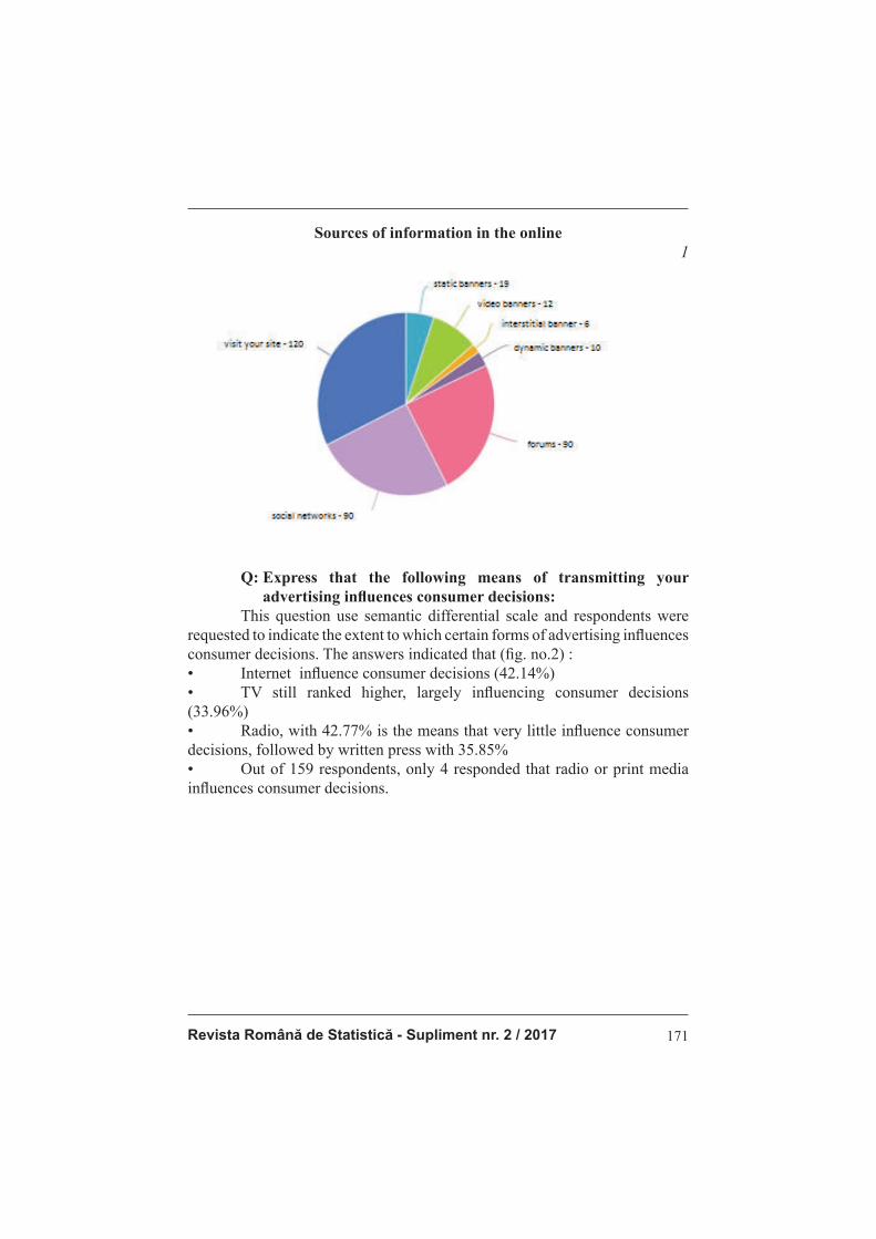
Revista Română de Statistică - Supliment nr. 2 / 2017 171

Sources of information in the online

Fig. no. 1

Q: Express that the following means of transmitting your

advertising infl uences consumer decisions:

This question use semantic differential scale and respondents were requested to indicate the extent to which certain forms of advertising infl uences consumer decisions. The answers indicated that (fi g. no.2) :• Internet infl uence consumer decisions (42.14%)

• TV still ranked higher, largely infl uencing consumer decisions

(33.96%)

• Radio, with 42.77% is the means that very little infl uence consumer

decisions, followed by written press with 35.85%

• Out of 159 respondents, only 4 responded that radio or print media

infl uences consumer decisions.

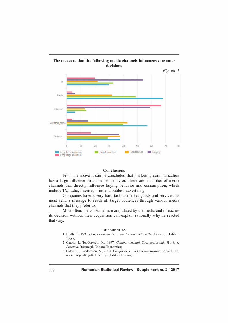
Romanian Statistical Review - Supplement nr. 2 / 2017172

The measure that the following media channels infl uences consumer

decisions

Fig. no. 2

Conclusions

From the above it can be concluded that marketing communication has a large infl uence on consumer behavior. There are a number of media channels that directly infl uence buying behavior and consumption, which include TV, radio, Internet, print and outdoor advertising. Companies have a very hard task to market goods and services, as must send a message to reach all target audiences through various media channels that they prefer to. Most often, the consumer is manipulated by the media and it reaches its decision without their acquisition can explain rationally why he reacted that way.

REFERENCES

1. Blythe, J., 1998. Comportamentul consumatorului, ediția a II-a. București, Editura Teora;

2. Catoiu, I., Teodorescu, N., 1997. Comportamentul Consumatorului. Teorie şi

Practică, București, Editura Economică; 3. Catoiu, I., Teodorescu, N., 2004. Comportamentul Consumatorului, Ediţia a II-a,

revăzută şi adăugită. București, Editura Uranus;

Revista Română de Statistică - Supliment nr. 2 / 2017 173

4. Clergue, A., 2013. Să învățăm să ne tratăm fără medicamente. București, Editura Orizonturi;

5. Imbriale, R., 2007. Marketingul Motivaţional, Iasi, Editura Amsta Publishing; 6. Kotler, Ph., Keller, K.L., 1999. Managementul marketingului. București, Teora; 7. Minculete, G., 2007. Marketing. București, Editura Universităţii Naţionale de

Apărare “Carol I”;

8. Orzan, Gh., Orzan, M., 2007. Cybermarketing. Bucureşti, Uranus;

9. Popescu, I. C., 2003. Comunicarea în marketing – concepte, tehnici, strategii,

ediția a II-a revăzută și adăugită. București, Uranus;

10. Hanafi zadeh, M., Behboudi, M., 2012. Online advertising and promotion :

Modern Tehnologies for Marketing. SUA, IGI Global ;

11. Pickton, D., Broderick, A., 2005. Integrated Marketing Communications – second

edition. Prentice Hall, England ;

12. Rusu, C., 2009. Relationship Marketing-o soluţie pentru sistemul bancar

românesc?, The Romanian Economic Journal, Year XII, no. 34, pp. 145-166;

13. Weiss, B., 2007. Efectele publicității: Comunicare de piață de succes: instrumente,

reguli și exemple. (s.l.), Editura IAA.