anexoi - vliz.be · la primera parte de esta tesis doctoral (cap´ıtulos 1−3) abarca el estudio...
TRANSCRIPT


ANEXO I
D. Salvador Galvan Herrera Secretario del Departamento de Fısica
de la Universidad de Las Palmas de Gran Canaria,
CERTIFICA,
Que el Consejo de Doctores del Departamento en sesion extraordinaria
tomo el acuerdo de dar el consetimiento para su tramitacion a la tesis doc-
toral titulada ‘Breeze-forced oscillations and strongly nonlinear tide-generated
internal solitons’ presentada por el doctorando D. Borja Aguiar Gonzalez y
dirigida por los Doctores Angel Rodrıguez Santana, Theo Gerkema y Jesus
Cisneros Aguirre.
Y para que ası conste, y a efectos de lo previsto en el Art. N 6 del
Reglamento para la Elaboracion, Defensa, Tribunal y Evaluacion de Tesis
Doctorales de la Universidad de Las Palmas de Gran Canaria, firmo la presente
en Las Palmas de Gran Canaria, a 23 de Abril de 2013.
iii


ANEXO II
- PROGRAMA DE DOCTORADO EN OCEANOGRAFIA -
Departamento de Fısica
Bienio 2006 – 2008
Breeze-forced oscillations and stronglynonlinear tide-generated internal solitons
Oscilaciones forzadas por las brisas y ondas internas solitarias de
origen mareal fuertemente no lineales
Tesis Doctoral presentada por D. Borja Aguiar Gonzalez para obtener el
grado de Doctor por la Universidad de Las Palmas de Gran Canaria.
Dirigida por el Dr. Angel Rodrıguez Santana, el Dr. Theo Gerkema y el
Dr. Jesus Cisneros Aguirre.
El Director El Director El Director El Doctorando
Las Palmas de Gran Canaria a 23 de Abril de 2013
v


A mis padres Mappi e Ignacio
A mi hermano Jose


Thesis Preview
The present Thesis entitled ‘Breeze-forced oscillations and strongly non-
linear tide-generated internal solitons’ was developed at the Universidad de
Las Palmas de Gran Canaria and the Royal Netherlands Institute for Sea
Research. Financial support for this PhD study was provided by the Min-
istry of Science and Innovation (Spanish Government) through a FPU grant
awarded to D. Borja Aguiar Gonzalez, and the research project PROMECA
(CTM2008-04057/MAR), whose Chief Investigator is Dr. Angel Rodrıguez
Santana.
This PhD research has been co-supervised by Dr. Angel Rodrıguez San-
tana and Dr. Jesus Cisneros Aguirre from the Department of Physics at the
Universidad de Las Palmas de Gran Canaria, and Dr. Theo Gerkema from
the Department of Physical Oceanography at the Royal Netherlands Institute
for Sea Research.
The structure of the Thesis is organized as follows. The first half of the doc-
ument deals with breeze-forced oscillations. Chapter 1 introduces the ‘state of
the art’ on the study of this phenomenon. Next we present an observational
study on breeze-forced oscillations poleward of the critical latitude for diurnal-
inertial resonance along Chapters 2–3. The second half of the document is
devoted to modeling strongly nonlinear tide-generated internal solitons. Sub-
sequently, Chapter 4 provides the empirical and theoretical background on
the phenomenon of study. Chapter 5 presents the derivation of a theoretical
model on strongly nonlinear tide-generated internal solitons; and, Chapter 6
discusses on numerical experiments performed with the derived model. Con-
clusions and future research are presented in Chapter 7. Finally, a summary
in Spanish is included in Chapter 8 as required by the PhD Thesis Regulations
from the Universidad de Las Palmas de Gran Canaria (BOULPGC. Art. 2,
iii

Chap. 2, November 5th 2008). The references are listed at the end of the
document.
iv
Presentacion de la Tesis
La presente Tesis Doctoral se titula ‘Oscilaciones forzadas por las brisas y
ondas internas solitarias de origen mareal fuertemente no lineales’ y se ha de-
sarrollado entre la Universidad de Las Palmas de Gran Canaria y el Royal
Netherlands Institute for Sea Research. La financiacion ha procedido del
Ministerio de Ciencia e Innovacion (Gobierno de Espana) a traves de la con-
cesion de una beca del Programa de Formacion de Profesorado Universitario
(FPU) al doctorando D. Borja Aguiar Gonzalez, y del proyecto de investi-
gacion PROMECA (CTM2008-04057/MAR), del cual el Dr. Angel Rodrıguez
Santana es Investigador Principal.
Esta Tesis Doctoral ha sido codirigida por el Dr. Angel Rodrıguez Santana
y el Dr. Jesus Cisneros Aguirre, ambos del Departamento de Fısica de la
Universidad de Las Palmas de Gran Canaria, y por el Dr. Theo Gerkema del
Departamento de Oceanografıa Fısica del Royal Netherlands Institute for Sea
Research.
La estructura del documento se ha organizado de la siguiente manera. La
primera parte de la Tesis Doctoral (Capıtulos 1-3) investiga la respuesta del
oceano al forzamiento de las brisas. El Capıtulo 1 introduce el ‘estado del arte’
en el estudio de este fenomeno fısico. Los Capıtulos 2-3 forman el nucleo de
un estudio observacional sobre oscilaciones forzadas por las brisas en latitudes
crıticas para la resonancia diurno-inercial. La segunda parte de la Tesis Doc-
toral (Capıtulos 4-6) desarrolla un modelo teorico para la simulacion de ondas
internas solitarias de origen mareal fuertemente no lineales. El Capıtulo 4 in-
troduce el ‘estado del arte’ en el estudio de este fenomeno fısico. El Capıtulo 5
describe el desarrollo del modelo teorico. El Capıtulo 6 presenta la discusion de
diferentes simulaciones numericas obtenidas con el modelo. Las conclusiones
y trabajo futuro abarcan el contenido del Capıtulo 7. Por ultimo se incluye
v

un resumen en espanol de la Tesis Doctoral en el Capıtulo 8 para cumplir con
los requisitos establecidos por el Reglamento para la Elaboracion, Tribunal,
Defensa y Evaluacion de Tesis Doctorales de la Universidad de Las Palmas de
Gran Canaria (BOULPGC. Art. 2, Cap. 2, 5 de Noviembre de 2008). Las
referencias citadas a lo largo del documento figuran al final del mismo.
vi

Summary
The present thesis deals with observations of breeze-forced oscillations andmodeling of strongly nonlinear tide-generated internal solitons. These twophenomena are of special interest owing to its periodic appearance, speciallyin shelf areas, with associated highly energetic motions. The contents of theseven chapters which compose this thesis are distributed as follows.
The first half of the thesis (Chapters 1-3 ) is devoted to the study of breeze-forced oscillations around the critical latitudes for diurnal-inertial resonance.Chapter 1 contains an introduction to the various physical concepts surround-ing a breeze-forced scenario, i.e. sea-land breezes, near-inertial oscillations,periodic forcing and near-inertial resonance. In Chapter 2 we study the tem-poral evolution of resonant breeze-forced oscillations in coastal areas polewardof the critical latitude for diurnal-inertial resonance (30N/S). The research isbased on simultaneous and co-located meteorological and oceanographic datacollected from three REDEXT (Red Exterior de Boyas) buoys deployed aroundthe Iberian Peninsula: the Gulf of Cadiz, the Gulf of Valencia and the CapePenas area. With this aim, new applications of rotary wavelet analysis areperformed. In Chapter 3 we explore the role of breeze-forced-oscillations onpromoting diapycnal mixing processes. The measurements we used here weretaken during the Maritime Rapid Environmental Assessment 2004 (MREA04)sea trial off the west coast of the Iberian Peninsula and from a meteorologicalland station provided by the Instituto Hidrografico - Portugal. This researchprovides observational results of breeze-forced oscillations in the stratified wa-ters of the Bay of Setubal, framed within the critical latitudes (30±10 N/S),for diurnal-inertial resonance where they can greatly contribute to triggeringdiapycnal mixing.
The second half of the thesis (Chapters 4-6 ) focuses on the modeling ofstrongly nolinear tide-generated internal solitons. Chapter 4 starts our re-
vii

Summary
search with an introduction to a solitons scenario in the ocean. Thereof, inChapter 5 we derive a new two-fluid layer model consisting of a set of forcedrotation-modified Boussinesq equations for studying the generation and evolu-tion of strongly nonlinear weakly nonhydrostatic dispersive interfacial waves.Next we develop and describe the numerical scheme used to solve the model.In Chapter 6, a set of numerical experiments is presented and discussed. Theresults of this chapter validate the model as a useful tool for exploring andinterpreting the conditions under which full nonlinearity effects become im-portant for soliton generation.
Chapter 7 closes this PhD study presenting an overview of the main scien-tific contributions and conclusions which arise from results and discussion ofthis work.
viii

Resumen
La presente Tesis Doctoral se centra en el estudio observacional de oscilacionesforzadas por las brisas y el modelaje de ondas internas solitarias de origenmareal fuertemente no lineales. El interes de estos fenomenos oceanograficosradica en su aparicion periodica, especialmente en ambientes de plataformacontinental, con corrientes asociadas altamente energeticas. La estructura deeste trabajo de investigacion se encuentra dividida de la siguiente manera.
La primera parte de esta Tesis Doctoral (Capıtulos 1−3) abarca el estudioobservacional de oscilaciones forzadas por las brisas en latitudes crıticas parala resonancia diurno-inercial (30±10 N/S). El Capıtulo 1 contiene una intro-duccion al fenomeno de las oscilaciones forzadas por las brisas. El Capıtulo 2 sebasa en medidas simultaneas de datos meteorologicos y oceanograficos proce-dentes de tres boyas REDEXT (Red Exterior de Boyas) localizadas en el Golfode Cadiz, el Golfo de Valencia y en las proximidades del Cabo Penas. Conestas medidas, y aplicando la metodologıa de wavelet rotatoria, analizamos laevolucion temporal de oscilaciones forzadas por las brisas en latitudes que seencuentran por encima de la latitud crıtica para la resonancia diurno-inercial(30N/S). El Capıtulo 3 investiga el papel de las oscilaciones forzadas por lasbrisas en la generacion de procesos de mezcla diapicna. Los datos procedende la campana oceanografica Maritime Rapid Environmental Assessment 2004(MREA04), que tuvo lugar en la costa oeste de la Penınsula Iberica en Abrilde 2004, y de una estacion meteorologica costera del Instituto Hidrografico -Portugal.
La segunda parte de la Tesis (Capıtulos 4−6) trabaja el modelaje de ondasinternas solitarias de origen mareal fuertemente no lineales. El Capıtulo 4 con-tiene una introduccion al fenomeno de ondas internas solitarias en el oceano.El Capıtulo 5 describe el desarrollo teorico empleado para derivar un nuevomodelo de generacion de ondas internas solitarias fuertemente no lineales y
ix

Resumen
debilmente no hidrostaticas. Se detalla ademas el esquema numerico aplicadopara resolver el modelo. Por ultimo, el Capıtulo 6 presenta una serie de ex-perimentos numericos que validan el modelo como una herramienta util paraexplorar e interpretar las condiciones bajo la cuales los efectos fuertemente nolineales de las ondas internas solitarias se consideran determinantes para laadecuada simulacion del fenomeno.
El Capıtulo 7 presenta las principales contribuciones y conclusiones delpresente trabajo de investigacion, ası como futuras lıneas de trabajo.
x
Contents
List of Figures xv
1 Introduction to a Breeze-Forced Scenario 11.1 Sea-Land Breezes . . . . . . . . . . . . . . . . . . . . . . . . . . 11.2 Breeze-Forced Oscillations . . . . . . . . . . . . . . . . . . . . . 7
1.2.1 Periodic Forcing and Near-Inertial Resonance . . . . . . 131.2.2 Stratification and Vertical Mixing . . . . . . . . . . . . 19
1.3 Scope of the Study . . . . . . . . . . . . . . . . . . . . . . . . . 22
2 Breeze-Forced Oscillations Poleward of the Critical Latitudefor Diurnal-Inertial Resonance 252.1 Outline . . . . . . . . . . . . . . . . . . . . . . . . . . . . . . . 252.2 Data and Methodology . . . . . . . . . . . . . . . . . . . . . . . 262.3 Results and Discussion . . . . . . . . . . . . . . . . . . . . . . . 29
2.3.1 Characterization of Three Wind-Forced Scenarios . . . . 292.3.2 The Ocean Response to Diurnal Wind Forcing: A Ro-
tary Analysis . . . . . . . . . . . . . . . . . . . . . . . . 382.4 Conclusions . . . . . . . . . . . . . . . . . . . . . . . . . . . . . 46
3 Breeze-Forced Oscillations and Diapycnal Mixing 493.1 Outline . . . . . . . . . . . . . . . . . . . . . . . . . . . . . . . 493.2 Data and Methodology . . . . . . . . . . . . . . . . . . . . . . . 513.3 Results and Discussion . . . . . . . . . . . . . . . . . . . . . . . 54
3.3.1 A Breeze-Forced Scenario . . . . . . . . . . . . . . . . . 543.3.2 Breeze-Forced Oscillations . . . . . . . . . . . . . . . . . 563.3.3 Diapycnal Mixing and Breeze-Forced Events . . . . . . . 593.3.4 Impact of BFOs in the Bay of Setubal . . . . . . . . . . 65
3.4 Conclusions . . . . . . . . . . . . . . . . . . . . . . . . . . . . . 66
xi
CONTENTS
4 Introduction to a Solitons Scenario 714.1 Solitary Waves in the Ocean . . . . . . . . . . . . . . . . . . . . 714.2 A Mathematical Approach to Solitons . . . . . . . . . . . . . . 784.3 Scope of the Study . . . . . . . . . . . . . . . . . . . . . . . . . 85
5 A Model for the Generation of Strongly Nonlinear, WeaklyNonhydrostatic Interfacial Waves 875.1 Outline . . . . . . . . . . . . . . . . . . . . . . . . . . . . . . . 875.2 Preliminaries . . . . . . . . . . . . . . . . . . . . . . . . . . . . 885.3 Scaling . . . . . . . . . . . . . . . . . . . . . . . . . . . . . . . . 895.4 Vertically Integrated Equations . . . . . . . . . . . . . . . . . . 91
5.4.1 Upper Fluid-Layer . . . . . . . . . . . . . . . . . . . . . 915.4.2 Lower Fluid-Layer . . . . . . . . . . . . . . . . . . . . . 92
5.5 Expansion in δ . . . . . . . . . . . . . . . . . . . . . . . . . . . 945.5.1 Lowest Order . . . . . . . . . . . . . . . . . . . . . . . . 955.5.2 Next Order . . . . . . . . . . . . . . . . . . . . . . . . . 96
5.5.2.1 Pressure in Upper Layer . . . . . . . . . . . . 975.5.2.2 Pressure in Lower Layer . . . . . . . . . . . . . 99
5.6 The Generation Model . . . . . . . . . . . . . . . . . . . . . . . 1015.7 Numerical Modeling . . . . . . . . . . . . . . . . . . . . . . . . 105
5.7.1 Numerical Strategy . . . . . . . . . . . . . . . . . . . . . 1055.7.2 Preliminaries to Solve u1 . . . . . . . . . . . . . . . . . 1115.7.3 Summary of Equations . . . . . . . . . . . . . . . . . . . 120
6 Numerical Experiments Solitons 1236.1 Outline . . . . . . . . . . . . . . . . . . . . . . . . . . . . . . . 1236.2 Configuration of the Numerical Experiments . . . . . . . . . . . 124
6.2.1 The Two-Fluid Layer System . . . . . . . . . . . . . . . 1246.2.2 Setting the Space-Time Grid . . . . . . . . . . . . . . . 1266.2.3 Basic Tests . . . . . . . . . . . . . . . . . . . . . . . . . 1276.2.4 Set of Experiments . . . . . . . . . . . . . . . . . . . . . 129
6.3 Generation of the Linear Hydrostatic Internal Tide . . . . . . . 1306.4 Generation of Strongly Nonlinear Solitons . . . . . . . . . . . . 134
6.4.1 ‘Table-Top’ Solitons (Rotationless Test, µ = 0) . . . . . 1346.4.2 Solitons with Two Layers of Equal Thickness (Rotation-
less Test, µ = 0) . . . . . . . . . . . . . . . . . . . . . . 1366.4.3 Strongly Nonlinear Solitons dispersed by the Effects of
the Earth’s Rotation . . . . . . . . . . . . . . . . . . . . 1376.5 Conclusions . . . . . . . . . . . . . . . . . . . . . . . . . . . . . 139
xii
CONTENTS
7 Conclusions and Future Research 141
A Rotary Wavelet Method 143A.1 Rotary Wavelet Power Spectrum . . . . . . . . . . . . . . . . . 143A.2 Rotary Coefficient . . . . . . . . . . . . . . . . . . . . . . . . . 145A.3 Statistical Significance Test . . . . . . . . . . . . . . . . . . . . 146A.4 Cross-Rotary Wavelet Power Spectrum . . . . . . . . . . . . . . 147A.5 Rotary Wavelet Coherence Squared Spectrum . . . . . . . . . . 147A.6 Rotary Wavelet Phase Spectrum . . . . . . . . . . . . . . . . . 148
B Theorem for Derivatives of Integrals with Variable Bound-aries 151
C Derivation of Function Gi(x, t) 153C.1 Upper Layer . . . . . . . . . . . . . . . . . . . . . . . . . . . . . 153C.2 Lower Layer Over an Oscillating Topography . . . . . . . . . . 155
D Derivation of(
∂p′2(1)
∂x
)159
E Substituting u2 in terms of u1 161
References 165
Data Acknowledgements 179
Agradecimientos 181
Curriculum Vitae 185
xiii

CONTENTS
xiv

List of Figures
1.1 Diagram of a Lake Breeze Regime . . . . . . . . . . . . . . . . 21.2 Diagram of a Land Breeze Regime . . . . . . . . . . . . . . . . 31.3 Seasonal Variability of Sea-land Breezes on the Texas-Louisiana
shelf . . . . . . . . . . . . . . . . . . . . . . . . . . . . . . . . . 51.4 The Effect of Coastlines on Sea Breezes . . . . . . . . . . . . . 71.5 Seasonal Variability of Breeze-Forced Oscillations on the Texas-
Louisiana shelf . . . . . . . . . . . . . . . . . . . . . . . . . . . 91.6 Breeze-Forced Oscillations on the Namibian shelf . . . . . . . . 101.7 Phase Evolution of Breeze-Forced and Free Near-Inertial Oscil-
lations . . . . . . . . . . . . . . . . . . . . . . . . . . . . . . . . 121.8 Slab Model of Forced Oscillations . . . . . . . . . . . . . . . . . 141.9 A Continuos Model with Friction of Forced Oscillations . . . . 181.10 Effects of Breeze-Forced Oscillations on the Vertical Mixing . . 211.11 Regions for Diurnal/Semidiurnal Resonance . . . . . . . . . . . 23
2.1 Oceanographic Buoys - Puertos del Estado . . . . . . . . . . . 272.2 Rotary Wavelet Power Spectrum of Wind at the Buoy Gulf of
Cadiz . . . . . . . . . . . . . . . . . . . . . . . . . . . . . . . . 312.3 Rotary Wavelet Power Spectrum of Wind at the Buoy Valencia II 322.4 Rotary Wavelet Power Spectrum of Wind at the Buoy Cape
Penas . . . . . . . . . . . . . . . . . . . . . . . . . . . . . . . . 332.5 Rotary Wavelet Power Spectrum of Currents at the Buoy Gulf
of Cadiz . . . . . . . . . . . . . . . . . . . . . . . . . . . . . . . 342.6 Rotary Wavelet Power Spectrum of Currents at the Buoy Va-
lencia II . . . . . . . . . . . . . . . . . . . . . . . . . . . . . . . 352.7 Rotary Wavelet Power Spectrum of Currents at the Buoy Cape
Penas . . . . . . . . . . . . . . . . . . . . . . . . . . . . . . . . 36
xv
LIST OF FIGURES
2.8 Averaged Wavelet Variance of Wind and Currents from theBuoy at the Gulf of Cadiz . . . . . . . . . . . . . . . . . . . . . 39
2.9 Averaged Wavelet Variance of Wind and Currents from theBuoy at the Gulf of Valencia . . . . . . . . . . . . . . . . . . . 40
2.10 Averaged Wavelet Variance of Wind and Currents from theBuoy at the Cape Penas area . . . . . . . . . . . . . . . . . . . 41
2.11 Squared Wavelet Coherency and Phase Spectra between Windand Currents (Clockwise Components) measured at the BuoyGulf of Cadiz . . . . . . . . . . . . . . . . . . . . . . . . . . . . 43
2.12 Squared Wavelet Coherency and Phase Spectra between Windand Current (Clockwise Components) measured at the BuoyCape Penas . . . . . . . . . . . . . . . . . . . . . . . . . . . . . 45
3.1 MREA04 Data Set . . . . . . . . . . . . . . . . . . . . . . . . . 513.2 Wind Time series for the Bay of Setubal . . . . . . . . . . . . . 553.3 Breeze-Forced Oscillations on the Portuguese shelf . . . . . . . 573.4 Surface Contours for the Bay of Setubal . . . . . . . . . . . . . 603.5 Diapycnal Mixing Analysis . . . . . . . . . . . . . . . . . . . . 623.6 Rotary Wavelet Power Spectrum of Wind from a Meteorological
Station at Sines . . . . . . . . . . . . . . . . . . . . . . . . . . . 66
4.1 Schematic of Canonical Soliton Packets . . . . . . . . . . . . . 724.2 Solitary Waves over the Oregon shelf . . . . . . . . . . . . . . . 744.3 Evolution of a Solitons Packet in the Sulu Sea . . . . . . . . . . 754.4 Remote Sensing SAR (Synthetic Aperture Radar) images of
Solitons in the Sulu Sea . . . . . . . . . . . . . . . . . . . . . . 774.5 Solitary wave solutions of the eKdV equation . . . . . . . . . . 824.6 Comparison of KdV and MCC theories . . . . . . . . . . . . . . 83
6.1 Configuration of the Numerical Experiments . . . . . . . . . . . 1256.2 Moving Topography vs. Tidal Motion . . . . . . . . . . . . . . 1286.3 Generation of the Linear Hydrostatic Internal Tide (Rotation-
less case, µ = 0) . . . . . . . . . . . . . . . . . . . . . . . . . . . 1316.4 Generation of the Linear Hydrostatic Internal Tide (at Mid
Latitudes: φ = 45, µ = 4.61) . . . . . . . . . . . . . . . . . . . 1326.5 Generation of the Linear Hydrostatic Internal Tide (at High
Latitudes: φ = 90, µ = 6.52) . . . . . . . . . . . . . . . . . . . 1336.6 Generation of ‘Table-Top’ Solitons . . . . . . . . . . . . . . . . 1356.7 Time evolution of ‘Table-Top’ Solitons . . . . . . . . . . . . . . 136
xvi

LIST OF FIGURES
6.8 Generation of Solitons between Two Layers of Equal Thickness 1376.9 Time evolution of Solitons between Two Layers of Equal Thick-
ness . . . . . . . . . . . . . . . . . . . . . . . . . . . . . . . . . 1376.10 Time evolution of Strongly Nonlinear Solitons dispersed by the
Effects of the Earth’s Rotation (at Mid Latitudes: φ = 45,µ = 4.61) . . . . . . . . . . . . . . . . . . . . . . . . . . . . . . 138
xvii

LIST OF FIGURES
xviii
Chapter 1
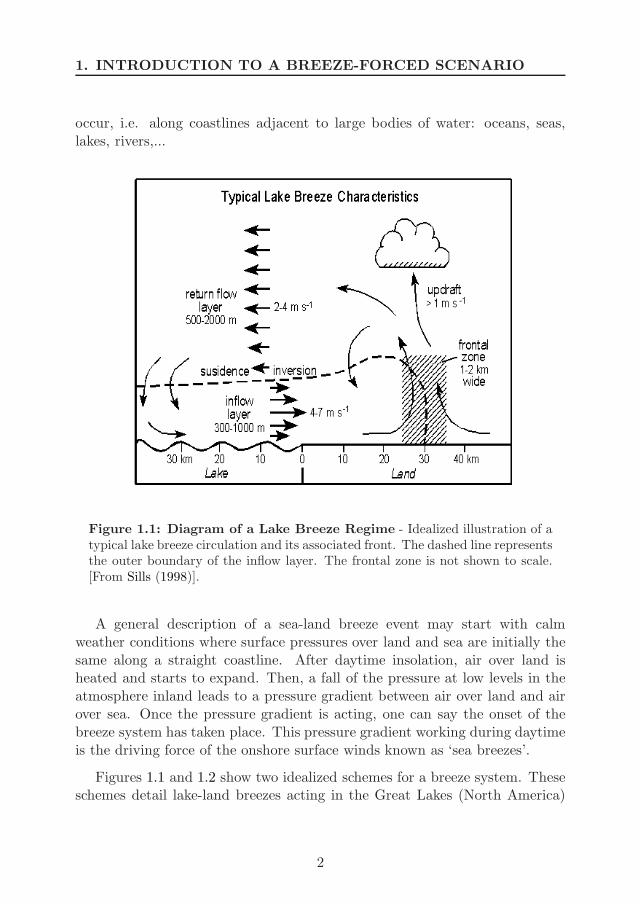
Introduction to aBreeze-Forced Scenario
This chapter presents a review on observations, theoretical and modeling worksfrom the existing literature on the topic ‘breeze-forced oscillations within thecritical latitudes for diurnal-inertial resonance’, which for short we may referin future chapters as ‘resonant breeze-forced oscillations’. In Section 1.1 westart the introduction to a breeze-forced scenario with a brief description ofthe fundamental aspects of sea-land breezes as a forcing to the coastal ocean.Therein, we focus on the physics of resonant breeze-forced oscillations in Sec-tion 1.2. We discuss the scope of this PhD study within the described contextin Section 1.3.
1.1 Sea-Land Breezes
Sea-land breezes are thermally-induced winds caused by the differential heat-ing and cooling of sea and land at diurnal cycles. This phenomenon is sup-ported due to the ocean has a higher specific heat capacity than land, whatentails that during daytime land warms up more than the ocean and so theair above it. The process reverses at night time, when land cools more thanthe ocean. This results in land-water air pressure differences driving systemsof breezes, generally onshore-offshore, along about two thirds of the earth’scoasts (Simpson, 1994). Thus we have the scenario where sea-land breezes can
1
1. INTRODUCTION TO A BREEZE-FORCED SCENARIO
occur, i.e. along coastlines adjacent to large bodies of water: oceans, seas,lakes, rivers,...
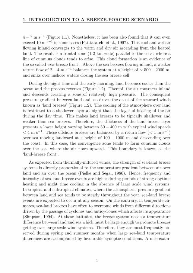
Figure 1.1: Diagram of a Lake Breeze Regime - Idealized illustration of atypical lake breeze circulation and its associated front. The dashed line representsthe outer boundary of the inflow layer. The frontal zone is not shown to scale.[From Sills (1998)].
A general description of a sea-land breeze event may start with calmweather conditions where surface pressures over land and sea are initially thesame along a straight coastline. After daytime insolation, air over land isheated and starts to expand. Then, a fall of the pressure at low levels in theatmosphere inland leads to a pressure gradient between air over land and airover sea. Once the pressure gradient is acting, one can say the onset of thebreeze system has taken place. This pressure gradient working during daytimeis the driving force of the onshore surface winds known as ‘sea breezes’.
Figures 1.1 and 1.2 show two idealized schemes for a breeze system. Theseschemes detail lake-land breezes acting in the Great Lakes (North America)
2
1.1 Sea-Land Breezes
based on previous literature values (Moroz, 1967; Lyons, 1972; Lyons and Ols-son, 1973; Keen and Lyons, 1978) and allow us to explain the main dynamicsof sea-land breezes. However, though thickness layer and velocity values main-tain rather similar numbers, it should be noticed that horizontal scales havebeen observed to be longer in oceanic areas in comparison with those in lake-land breeze systems (Simpson, 1994; Hyder et al., 2002; Rippeth et al., 2002;Simpson et al., 2002; Gille et al., 2003; Zhang et al., 2009; Hyder et al., 2011).Oceanic horizontal scales may extend from several tens to a few hundreds ofkilometres alongshore, and more than 100 km offshore from the coast (Simp-son, 1994; Gille et al., 2003; Aparna et al., 2005; Gille et al., 2005; Zhang et al.,2009).
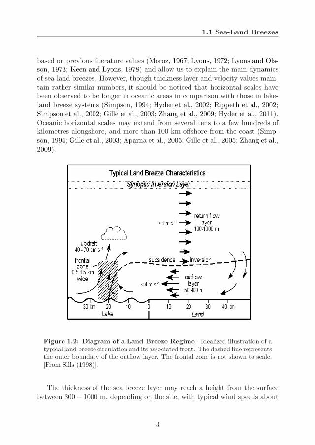
Figure 1.2: Diagram of a Land Breeze Regime - Idealized illustration of atypical land breeze circulation and its associated front. The dashed line representsthe outer boundary of the outflow layer. The frontal zone is not shown to scale.[From Sills (1998)].
The thickness of the sea breeze layer may reach a height from the surfacebetween 300− 1000 m, depending on the site, with typical wind speeds about
3
1. INTRODUCTION TO A BREEZE-FORCED SCENARIO
4− 7 m s−1 (Figure 1.1). Nonetheless, it has been also found that it can evenexceed 10 m s−1 in some cases (Pattiaratchi et al., 1997). This cool and wet airflowing inland converges to the warm and dry air ascending from the heatedland. The result is a frontal zone (1-2 km wide) parallel to the coast where aline of cumulus clouds tends to arise. This cloud formation is an evidence ofthe so called ‘sea-breeze front’. Above the sea breezes flowing inland, a weakerreturn flow of 2− 4 m s−1 balances the system at a height of ∼ 500− 2000 m,and sinks over inshore waters closing the sea breeze cell.
During the night time and the early morning, land becomes cooler than theocean and the process reverses (Figure 1.2). Thereof, the air contracts inlandand descends creating a zone of relatively high pressure. The consequentpressure gradient between land and sea drives the onset of the seaward windsknown as ‘land breezes’ (Figure 1.2). The cooling of the atmosphere over landis restricted to a shallower layer at night than the layer of heating of the airduring the day time. This makes land breezes to be tipically shallower andweaker than sea breezes. Therefore, the thickness of the land breeze layerpresents a lower height varying between 50 − 400 m with typical wind speeds< 4 m s−1. These offshore breezes are balanced by a return flow (< 1 m s−1)over sea moving landward at a height of 100 − 1000 m and descending overthe coast. In this case, the convergence zone tends to form cumulus cloudsover the sea, where the air flows upward. This boundary is known as the‘land-breeze front’.
As expected from thermally-induced winds, the strength of sea-land breezesystems is directly proportional to the temperature gradient between air overland and air over the ocean (Pielke and Segal, 1986). Hence, frequency andintensity of sea-land breeze events are higher during periods of strong daytimeheating and night time cooling in the absence of large scale wind systems.In tropical and subtropical climates, where the atmospheric pressure gradientbetween land and sea tends to be steady throughout the year, sea-land breezeevents are expected to occur at any season. On the contrary, in temperate cli-mates, sea-land breezes have often to overcome winds from different directionsdriven by the passage of cyclones and anticyclones which affects its appearance(Simpson, 1994). At these latitudes, the breeze system needs a temperaturedifference between land and sea which must be large enough to promote breezesgetting over large scale wind systems. Therefore, they are most frequently ob-served during spring and summer months when large sea-land temperaturedifferences are accompanied by favourable synoptic conditions. A nice exam-
4

1.1 Sea-Land Breezes
ple of seasonal variability for sea-land breezes is shown in Zhang et al. (2009)for the Texas-Lousiana shelf (Figure 1.3). They use a wavelet power spectrumof the eastwest wind component to evaluate the temporal evolution of thewind variance at a location on the shelf from December 1997 to April 2004.As it can be seen from the spectrum, the magnitude of diurnal wind variance,mainly associated with sea breeze, peaks in summer months (June-August)and is weaker during the nonsummer months (September-May) (Zhang et al.,2009).
Figure 1.3: Seasonal Variability of Sea-land Breezes on the Texas-Louisiana shelf - (top) Wavelet power spectrum (unitless) of the normalized10-m eastwest wind component (mean value was subtracted from the time seriesand then normalized by the standard deviation) at NDBC buoy station PTAT2(27.838N, 97.058W). Only significant values are plotted, which are >95% confi-dence for a red-noise process with a lag-1 coefficient of 0.72 (Torrence and Compo1998). (bottom) The gray solid curve is the frequency- (period) averaged waveletvariance time series (m2 s−2) over the 0.831.17 cpd band during the observa-tion period. The black solid curve is the 3-month low-passed values of the graycurve. The horizontal gray dashed line is the 95% confidence level. The blackbars indicate summer periods. [From Zhang et al. (2009) - Fig. 2].
5

1. INTRODUCTION TO A BREEZE-FORCED SCENARIO
Along a straight coastline and over a flat terrain, the sea breeze initiallyextends out to sea as well as inland at right angles to the coast. Along the day-time, the breeze direction shifts a few degrees anticyclonically due to Earth’srotation and, after a period of time, may approach geostrophic balance flowingapproximately parallel to the coastline if the circulation is long lived (Lyons,1972), particularly at offshore locations. The period of time the breeze direc-tion would take for this shift is related with the Coriolis parameter and sodepends on the latitude. Land breezes, in contrast, are usually less shifted, nomore than 20-30.
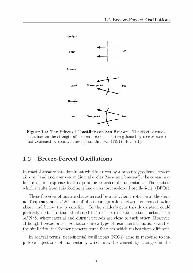
Nevertheless, most coastlines are irregular what induces areas of breezeconvergence and divergence. Hence, wherever the coast is not straight, theshape of the shoreline makes the result more complicate and the breezes flowwill not be uniform. Simpson (1994) showed in a simple diagram (Figure 1.4)how the sea breezes converges (the land breezes diverges) at convex coasts;and, inversely, the sea breezes diverges (the land breezes converges) when thecoast is concave. Accordingly, convergences zones which promotes strong seabreezes during daytime (and weaker divergent land breezes at night) can befound in capes, peninsulas, etc. And divergent sea breezes (convergent landbreezes) occurr more frequently in bays, gulfs, etc.
Wind shifts, in addtion to those produced by Earth’s rotation and irregu-larities along the coastline, may be also produced by the presence of coastaltopography. This effect tends to shift the sea-breeze direction later in the daytowards the main heated land mass further inland. All these factors togethermake the behaviour of a sea-land breeze event to be not straightforward. Theresult can be as surprising as we may find breezes rotating at different sensesover relatively close areas, oscillating even against Earth’s rotation (Simpson,1994).
The fact of sea-land breeze systems are not determined by solely one as-pect, but depend on the interaction of several local factors, presents importantconsequences on forcing the coastal ocean. As one can imagine, a clockwiserotating wind system will not produce the same ocean response at a given lati-tude than a counterclockwise rotating wind. Thus, an appropiate methodolgywhich allow us to characterize in time-frequency space both the amplitude androtating properties of sea-land breezes is crucial to further explore dynamicsof breeze-forced oscillations in the ocean. On the basis of these arguments,we find rotary wavelet method (Appendix A) a suitable option to this kind ofstudies, though to our knowledge it has no been yet applied in the literature.
6
1.2 Breeze-Forced Oscillations
Figure 1.4: The Effect of Coastlines on Sea Breezes - The effect of curvedcoastlines on the strength of the sea breeze. It is strengthened by convex coastsand weakened by concave ones. [From Simpson (1994) - Fig. 7.1].
1.2 Breeze-Forced Oscillations
In coastal areas where dominant wind is driven by a pressure gradient betweenair over land and over sea at diurnal cycles (‘sea-land breezes’), the ocean maybe forced in response to this periodic transfer of momentum. The motionwhich results from this forcing is known as ‘breeze-forced oscillations’ (BFOs).
These forced-motions are characterized by anticyclonic rotation at the diur-nal frequency and a 180 out of phase configuration between currents flowingabove and below the pycnocline. To the reader’s eyes this description couldperfectly match to that attributed to ‘free’ near-inertial motions acting near30N/S, where inertial and diurnal periods are close to each other. However,although breeze-forced oscillations are a type of near-inertial motions, and sothe similarity, the former presents some features which makes them different.
In general terms, near-inertial oscillations (NIOs) arise in response to im-pulsive injections of momentum, which may be caused by changes in the
7
1. INTRODUCTION TO A BREEZE-FORCED SCENARIO
wind stress vector (Pollard and Millard, 1970) or by the transient responsein a geostrophic adjustment process (Gill, 1984). The resulting motions aredriven by a dynamic balance between the geostrophic and radial accelerations,which makes them rotate anticyclonically at the local inertial frequency f. Thesurface-generated oscillations are consequently more energetic in the surfacelayers, and propagates downwards through the water column via internal fric-tion (Qi et al., 1995). Consequently, there is an increasing phase delay anddecresing energy with depth relative to near-inertial currents rotating at shal-lower layers. The vertical structure is thus characterized by a first baroclinicmode with a phase shift of ∼ 180 between surface and bottom layers (Millotand Crepon, 1981; Orlic, 1987; Salat et al., 1992; Knight et al., 2002). These‘free’ motions may last for many oscillatory cycles, especially in regions wherethe frictional damping is weak.
On the contrary, breeze-forced oscillations are ‘periodic’ inertial motions inresponse to a more regular forcing close to the inertial frequency (Hyder et al.,2011). At first, the ocean response seems analogous to that exhibited by ‘free’near-inertial oscillations, anticyclonic currents rotating phase-shifted aboveand below the pycnocline. Nevertheless, these wind-generated oscillations nearcoastal areas differ from purely near-inertial oscillations in several aspects thatwe describe now, and which respond to the nature of its driving force: the sea-land breezes.
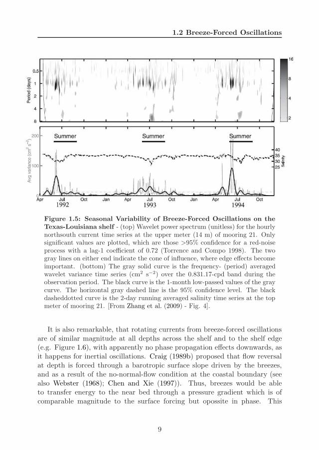
Regarding to its time variability, breeze-forced oscillations are of higherappearance and intensity during summer months, according to its forcing vari-ability. Throughout this seasonal period, atmospheric pressure gradient dueto enhanced diurnal heating and cooling cycles promotes stronger breezes withuninterrupted phase, and subsequently the transfer of energy to the ocean re-sults in a diurnal band which is highly enriched within the kinetic spectrum.For instance, Zhang et al. (2009) examine the breeze-forced oscillation vari-ability on the Texas-Lousiana shelf (TLS) using wavelet analysis. Thus, theypresented the wavelet power spectrum of the north-south current time seriesat 14 m in order to highlight how the diurnal-inertial band (DIB) peaks insummer compared to nonsummer seasons (Figure 1.5). In their analysis theyalso found that, while stratification helps the enhacement of the DIB currentvariance, the deepening of the mixed layer depth appears to weaken it (Zhanget al., 2009).
8
1.2 Breeze-Forced Oscillations
Figure 1.5: Seasonal Variability of Breeze-Forced Oscillations on theTexas-Louisiana shelf - (top) Wavelet power spectrum (unitless) for the hourlynorthsouth current time series at the upper meter (14 m) of mooring 21. Onlysignificant values are plotted, which are those >95% confidence for a red-noiseprocess with a lag-1 coefficient of 0.72 (Torrence and Compo 1998). The twogray lines on either end indicate the cone of influence, where edge effects becomeimportant. (bottom) The gray solid curve is the frequency- (period) averagedwavelet variance time series (cm2 s−2) over the 0.831.17-cpd band during theobservation period. The black curve is the 1-month low-passed values of the graycurve. The horizontal gray dashed line is the 95% confidence level. The blackdasheddotted curve is the 2-day running averaged salinity time series at the topmeter of mooring 21. [From Zhang et al. (2009) - Fig. 4].
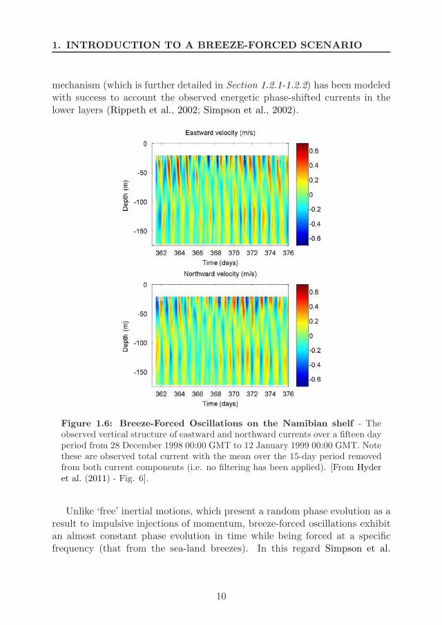
It is also remarkable, that rotating currents from breeze-forced oscillationsare of similar magnitude at all depths across the shelf and to the shelf edge(e.g. Figure 1.6), with apparently no phase propagation effects downwards, asit happens for inertial oscillations. Craig (1989b) proposed that flow reversalat depth is forced through a barotropic surface slope driven by the breezes,and as a result of the no-normal-flow condition at the coastal boundary (seealso Webster (1968); Chen and Xie (1997)). Thus, breezes would be ableto transfer energy to the near bed through a pressure gradient which is ofcomparable magnitude to the surface forcing but opossite in phase. This
9
1. INTRODUCTION TO A BREEZE-FORCED SCENARIO
mechanism (which is further detailed in Section 1.2.1-1.2.2) has been modeledwith success to account the observed energetic phase-shifted currents in thelower layers (Rippeth et al., 2002; Simpson et al., 2002).
Figure 1.6: Breeze-Forced Oscillations on the Namibian shelf - Theobserved vertical structure of eastward and northward currents over a fifteen dayperiod from 28 December 1998 00:00 GMT to 12 January 1999 00:00 GMT. Notethese are observed total current with the mean over the 15-day period removedfrom both current components (i.e. no filtering has been applied). [From Hyderet al. (2011) - Fig. 6].
Unlike ‘free’ inertial motions, which present a random phase evolution as aresult to impulsive injections of momentum, breeze-forced oscillations exhibitan almost constant phase evolution in time while being forced at a specificfrequency (that from the sea-land breezes). In this regard Simpson et al.
10
1.2 Breeze-Forced Oscillations
(2002) show an illustrative example for a breeze forcing which is interrupted(after day 31 in Figure 1.7) and the resultant motion switches to the inertialfrequency so that, when viewed as a diurnal-forced motion, there is a regularincrease in the phase lag with time (Figure 1.7). Thus the alternation ofdiurnal-forced and transient-inertial oscillations is an expected feaure of wind-forced motions. Additionally, some authors Hyder et al. (2002); Rippeth et al.(2002); Sobarzo et al. (2007); Hyder et al. (2011) have also observed in timeseries data that there is a beat period of ∼ (2π/(ω − f) in which the strengthof the periodic diurnal current components (ω) oscillates in combinaton withfree phase inertial current components (f).
Geographically, near-inertial motions are a widespread feature in deep andcoastal oceans which brings into play an important source of energy availablefor mixing (Webster, 1968; Millot and Crepon, 1981; Salat et al., 1992; Fontet al., 1995; van Haren et al., 1999; Knight et al., 2002; van Aken et al.,2005; Sobarzo et al., 2007; Chaigneau et al., 2008). However, near-inertialenergy level is not uniform worlwide and is more variable than the rest of thespectrum (Fu, 1981; Garret, 2001; Gerkema and Shrira, 2005). Breeze-forcedoscillations contribute (among other phenomena not addressed here) to thosegeographical differences on the near-inertial energy levels. This is based onthe fact that depending on the latitude in which the breeze forcing is acting,the ocean response may be resonant. Thus, near 30 N/S, inertial and diurnalperiods are close to each other and the transfer of momentum and energy frombreeze forcing to inertial motions can be significantly increased (Hyder et al.,2002; Rippeth et al., 2002; Simpson et al., 2002; Sobarzo et al., 2007).
On the basis of all mentioned differences between breeze-forced oscillationsand ‘free’ near-inertial oscillations, valuable efforts have been done in the lastdecades to develop theory and model breeze-forced oscillations (Craig, 1989b;Chen and Xie, 1997; Rippeth et al., 2002; Simpson et al., 2002; Hyder et al.,2002, 2011). In the following, we review theoretical and modeling works whichfocus on the observed behaviour of the ocean to breeze forcing. Additionally,we point out those modeling results which predict interesting features not yetconfirmed with observations and thus needed of further research. This reviewprovides a deeper insight into the physics behind the generation and evolutionof breeze-forced oscillations.
11

1. INTRODUCTION TO A BREEZE-FORCED SCENARIO
Figure 1.7: Phase Evolution of Breeze-Forced and Free Near-InertialOscillations - Amplitude and phase of the diurnal motion over the full recordingperiod. (a) Current at 34-m anticlockwise (*) and clockwise (+), (b) current at126 m anticlockwise (x) and clockwise (•), (c) phase of anticlockwise componentat 34 m (*) and 126 m (x), (d) wind amplitude as anticlockwise (*) and clockwise(+) components, and (e) phase of the wind components (*) anticlockwise andclockwise (+). The straight sloping line in (c) indicates the rate of phase changeof a pure inertial oscillation (15.5 d−1). [From Simpson et al. (2002) - Fig. 7].
12

1.2 Breeze-Forced Oscillations
1.2.1 Periodic Forcing and Near-Inertial Resonance
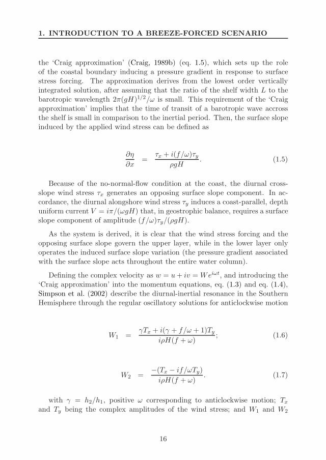
Theoretical and modeling advances on the ocean response produced by pe-riodic forcing (tidal and wind forcing) at a particular frequency have beengreatly benefited from the studies of Battisti and Clarke (1982) and Craig(1989a,b). In the following we describe the dynamics of breeze-forced oscilla-tions by introducing some recent illuminating works.
Critical Latitudes for Resonance
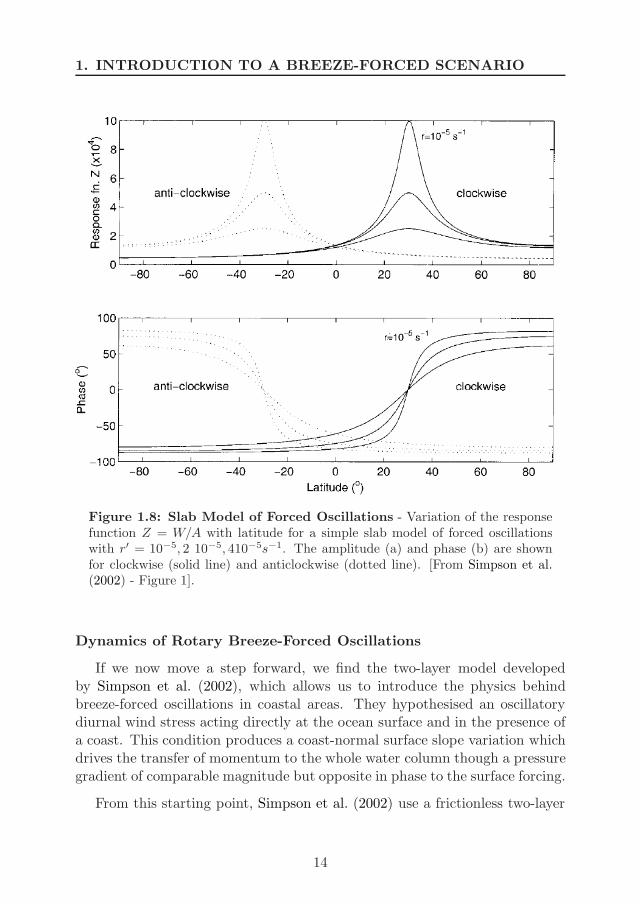
The essential mechanism and latitudinal variation of diurnal wind-forcedmotions are clearly illustrated in Simpson et al. (2002) with a simple slabmodel for a water column of depth H vertically uniform in velocity forcedby an oscillating wind stress τs with no horizontal pressure gradients (Fig-ure 1.8). Frictional damping is introduced linearly via (−ru,−rv), leaving thedynamical equations for the complex velocity w = u + iv as
∂w
∂t+ ifω =
−rw + τs
ρH(1.1)
Then, the complex amplitudes for clockwise (W−) and anticlowise (W+)forcing at frequency ω are
W− =A−
i(f − ω) + r′; W+ =
A+
i(f + ω) + r′(1.2)
where τs/(ρH) = A±e±ωt and r′ = r/(ρH). As it can be seen in Figure 1.8(top), the ocean response is resonant (W → A/r′) for the clockwise case atthe critical latitud of 30N where f = ω, and for the anticlockwise case at thecritical latitud of 30S where f = −ω. In other words, the ocean response isresonant when diurnal and inertial periods are close to each other. Under thesecircumstances, current and forcing are in phase and the transfer of momentumand energy is significantly enhanced. It is also shown that the phase of thecurrent changes rapidly between limiting values of +π/2 and −π/2 fartherthan 30N/S, and that this effect is sharper when using a higher coefficientfor frictional damping.
13
1. INTRODUCTION TO A BREEZE-FORCED SCENARIO
Figure 1.8: Slab Model of Forced Oscillations - Variation of the responsefunction Z = W/A with latitude for a simple slab model of forced oscillationswith r′ = 10−5, 2 10−5, 410−5s−1. The amplitude (a) and phase (b) are shownfor clockwise (solid line) and anticlockwise (dotted line). [From Simpson et al.(2002) - Figure 1].
Dynamics of Rotary Breeze-Forced Oscillations
If we now move a step forward, we find the two-layer model developedby Simpson et al. (2002), which allows us to introduce the physics behindbreeze-forced oscillations in coastal areas. They hypothesised an oscillatorydiurnal wind stress acting directly at the ocean surface and in the presence ofa coast. This condition produces a coast-normal surface slope variation whichdrives the transfer of momentum to the whole water column though a pressuregradient of comparable magnitude but opposite in phase to the surface forcing.
From this starting point, Simpson et al. (2002) use a frictionless two-layer
14
1.2 Breeze-Forced Oscillations
analytical model with the upper layer being forced by a diurnal wind stressand the opposing surface slope resulting from this wind forcing; and, the lowerlayer being forced solely by the surface slope. This external pressure gradientforces the lower layer leading to phase-shifted motions with relatively the sameamplitude as in the upper layer. The model successes on reproducing the keyfeatures of reported breeze-forced oscillations in the literature: anticycloniccurrents rotating ∼ 180 out of phase above and below the pycnocline withenergetic amplitudes of similar magnitud and almost constant phase withinevery layer (Chen et al., 1996; Rippeth et al., 2002; Simpson et al., 2002; Zhanget al., 2009; Hyder et al., 2011). In contrast to what is observed with freenear-inertial motions (Millot and Crepon, 1981; Orlic, 1987), which exhibitan increasing phase delay and less energetic currents in deeper waters dueto momentum is transferred downward through the shear stress described byclassical Ekman theory.
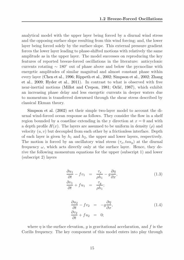
Simpson et al. (2002) set their simple two-layer model to account the di-urnal wind-forced ocean response as follows. They consider the flow in a shelfregion bounded by a coastline extending in the y direction at x = 0 and witha depth profile H(x). The layers are assumed to be uniform in density (ρ) andvelocity (u, v) but decoupled from each other by a frictionless interface. Depthof each layer is given by h1 and h2, the upper and lower layers, respectively.The motion is forced by an oscillatory wind stress (τx, tauy) at the diurnalfrequency ω, which acts directly only at the surface layer. Hence, they de-rive the following momentum equations for the upper (subscript 1) and lower(subscript 2) layers
∂u1
∂t− fv1 =
τx
ρh1− g
∂η
∂x, (1.3)
∂v1
∂t+ fu1 =
τy
ρh1;
∂u2
∂t− fv2 = −g
∂η
∂x, (1.4)
∂v2
∂t+ fu2 = 0;
where η is the surface elevation, g is gravitational accelaration, and f is theCorilis frequency. The key component of this model enters into play through
15
1. INTRODUCTION TO A BREEZE-FORCED SCENARIO
the ‘Craig approximation’ (Craig, 1989b) (eq. 1.5), which sets up the roleof the coastal boundary inducing a pressure gradient in response to surfacestress forcing. The approximation derives from the lowest order verticallyintegrated solution, after assuming that the ratio of the shelf width L to thebarotropic wavelength 2π(gH)1/2/ω is small. This requirement of the ‘Craigapproximation’ implies that the time of transit of a barotropic wave accrossthe shelf is small in comparison to the inertial period. Then, the surface slopeinduced by the applied wind stress can be defined as
∂η
∂x=
τx + i(f/ω)τy
ρgH. (1.5)
Because of the no-normal-flow condition at the coast, the diurnal cross-slope wind stress τx generates an opposing surface slope component. In ac-cordance, the diurnal alongshore wind stress τy induces a coast-parallel, depthuniform current V = iπ/(ωgH) that, in geostrophic balance, requires a surfaceslope component of amplitude (f/ω)τy/(ρgH).
As the system is derived, it is clear that the wind stress forcing and theopposing surface slope govern the upper layer, while in the lower layer onlyoperates the induced surface slope variation (the pressure gradient associatedwith the surface slope acts throughout the entire water column).
Defining the complex velocity as w = u + iv = Weiωt, and introducing the‘Craig approximation’ into the momentum equations, eq. (1.3) and eq. (1.4),Simpson et al. (2002) describe the diurnal-inertial resonance in the SouthernHemisphere through the regular oscillatory solutions for anticlockwise motion
W1 =γTx + i(γ + f/ω + 1)Ty
iρH(f + ω); (1.6)
W2 =−(Tx − if/ωTy)
iρH(f + ω). (1.7)
with γ = h2/h1, positive ω corresponding to anticlockwise motion; Tx
and Ty being the complex amplitudes of the wind stress; and W1 and W2
16
1.2 Breeze-Forced Oscillations
the complex amplitudes of the motion in upper and lower layer, respectively.Thus, the ocean response, eq. (1.6) and eq. (1.7), for the anticyclonic motionwill be enhanced at latitudes close to 30 S where it enters in resonance whithf → −ω so that f/ω → −1 leading to
W1 ≈ γTx + i(γ + iTy)
ρH(f + ω)≈ W2. (1.8)
This particular solution for the steady state response of the ocean nearcritical latitudes reproduces the main features of observed wind-forced diurnal-inertial oscillations that may be influenced by land boundaries (Chen et al.(1996); Rippeth et al. (2002); Simpson et al. (2002); Zhang et al. (2009);Hyder et al. (2011)). The phase of the forced-motion oscillating within thediurnal-inertial band is shifted by 180 between upper and lower layers, andthe velocity amplitude is of comparable magnitude in the two layers when thefactor γ, which is a function of the depth of the pycnocline, is of order unityas it occurrs in the study area of Simpson et al. (2002). Analogous effectsare obtained from the regular oscillatory solutions for clockwise motion in theNorthern Hemisphere (see Rippeth et al. (2002)). The ocean response is thenenhanced at latitudes close to 30 N where f → ω (Northern Hemisphere) andthe motion is resonant. In both hemispheres, the ocean response to cyclonicforcing at the diurnal frequency is remarkably weaker in the ratio | (f + ω) |/ | (f − ω |).
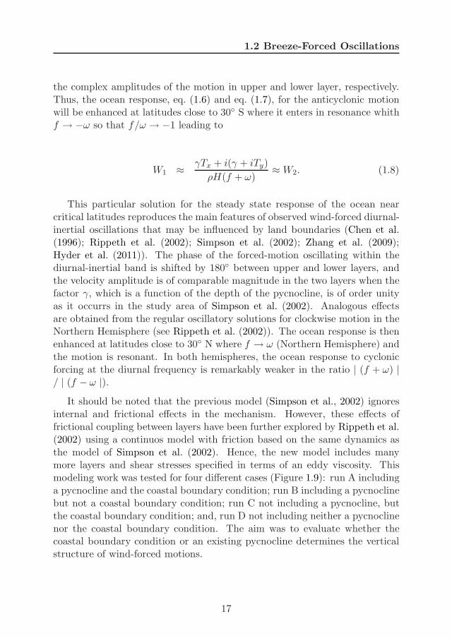
It should be noted that the previous model (Simpson et al., 2002) ignoresinternal and frictional effects in the mechanism. However, these effects offrictional coupling between layers have been further explored by Rippeth et al.(2002) using a continuos model with friction based on the same dynamics asthe model of Simpson et al. (2002). Hence, the new model includes manymore layers and shear stresses specified in terms of an eddy viscosity. Thismodeling work was tested for four different cases (Figure 1.9): run A includinga pycnocline and the coastal boundary condition; run B including a pycnoclinebut not a coastal boundary condition; run C not including a pycnocline, butthe coastal boundary condition; and, run D not including neither a pycnoclinenor the coastal boundary condition. The aim was to evaluate whether thecoastal boundary condition or an existing pycnocline determines the verticalstructure of wind-forced motions.
17
1. INTRODUCTION TO A BREEZE-FORCED SCENARIO
Figure 1.9: A Continuos Model with Friction of Forced Oscillations -Results from the continuous model. The predicted near surface (solid line) andnear bed (dotted line) along-shore current components. (a) Run A: results fromthe model run which includes a pycnocline and the coastal boundary condition.(b) Run B: results from the model run which includes a pycnocline but does notinclude a coastal boundary. (c) Run C: results from the model run which includesthe coastal boundary but no pycnocline. (d) Run D: results from the model runwith no coastal boundary or pycnocline. [From Rippeth et al. (2002) - Fig. 9].
Run results only reproduced the characteristic phase shift and the pen-etration of energy to near the bed in the cases where the coastal boundarycondition was included (run A and run C in Figure 1.9), whereas in its absence(run B and run D) forced motions did not exhibit these features. The authorsalso found that internal shear stresses did not greatly modify the frictionless
18
1.2 Breeze-Forced Oscillations
response to forcing (run A and run C), and confirmed that the reverse flow inthe lower layers primarily results from a barotropic pressure gradient (‘Craigapproximation’) set up by the applied wind stress and the no-normal-flow con-dition at the coastal boundary, which is the basis of the model. Consequently,these results point out that the upper and lower layers of breeze-forced mo-tions behave differently than those in purely inertial motions, where the outof phase layers are not driven by a constant forcing but by phase propagationeffects and the pycnocline has as well a main role in the propagation.
Modeling results from Rippeth et al. (2002) also find a beating cycle be-tween diurnal and inertial periods, despite using a diurnal forcing. In thecase of runs without a pycnocline (runs C-D), the beating dies after 4 daysas the transient signal is damped out, leaving a steady state diurnal periodsolution. This behaviour appear to be consistent with previously mentionedbeat periods found in observational data (Hyder et al., 2002; Sobarzo et al.,2007; Hyder et al., 2011).
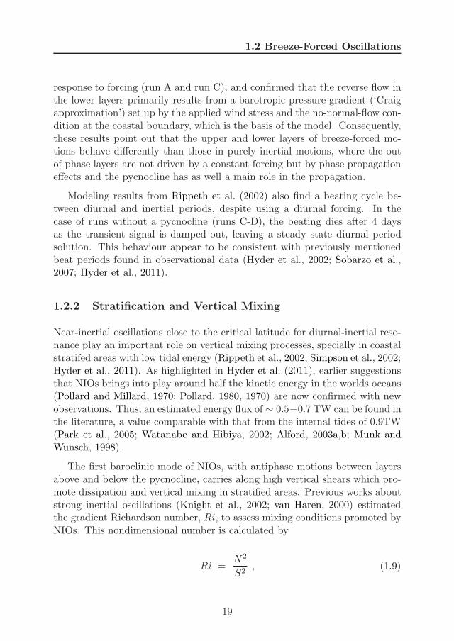
1.2.2 Stratification and Vertical Mixing
Near-inertial oscillations close to the critical latitude for diurnal-inertial reso-nance play an important role on vertical mixing processes, specially in coastalstratifed areas with low tidal energy (Rippeth et al., 2002; Simpson et al., 2002;Hyder et al., 2011). As highlighted in Hyder et al. (2011), earlier suggestionsthat NIOs brings into play around half the kinetic energy in the worlds oceans(Pollard and Millard, 1970; Pollard, 1980, 1970) are now confirmed with newobservations. Thus, an estimated energy flux of ∼ 0.5−0.7 TW can be found inthe literature, a value comparable with that from the internal tides of 0.9TW(Park et al., 2005; Watanabe and Hibiya, 2002; Alford, 2003a,b; Munk andWunsch, 1998).
The first baroclinic mode of NIOs, with antiphase motions between layersabove and below the pycnocline, carries along high vertical shears which pro-mote dissipation and vertical mixing in stratified areas. Previous works aboutstrong inertial oscillations (Knight et al., 2002; van Haren, 2000) estimatedthe gradient Richardson number, Ri, to assess mixing conditions promoted byNIOs. This nondimensional number is calculated by
Ri =N2
S2, (1.9)
19

1. INTRODUCTION TO A BREEZE-FORCED SCENARIO
where N2 is the squared Brunt-Vaisala frequency (squared buoyancy fre-quency), and S2 is the squared vertical current shear applied to a fluid parcel.The squared Brunt-Vaisala frequency is given by
N2 = − g
ρ0
∆ρ
∆z, (1.10)
where ρ is the potential density calculated from temperature and conduc-tivity data; g is the gravity constant; ρ0 is the averaged potential density; and∆z is the vertical distance between the top and the bottom of the fluid parcel.Finally, the vertical squared shear is given by
S2 =(∆u
∆z
)2+(∆u
∆z
)2, (1.11)
where ∆u and ∆v are the east-west and north-south current differencesbetween the top and bottom of the fluid parcel, respectively. Then, typicalvalues for Ri < 1 indicate the generation of Kelvin-Helmholtz instabilitiescaused by the vertical shear that triggers mixing in a stratified fluid (Miles,1986; Van Gastel and Pelegrı, 2004). On the contrary, if Ri >> 1, buoyancyis dominant since there is insufficient kinetic energy to homogenize the watercolumn.
Knight et al. (2002) estimated Ri using ADCP and CTD data in the NorthSea and found values less than 1 when strong inertial currents carried largevertical shears across the thermocline, although never approached to criticalvalues of 0.25. Dissipation measurements were also made and indicated thatmixing within the thermocline layer was more intense and was associated tohigh mean thermocline diffusion coefficients when large inertial current shearswere acting. Modeling results and observations in the North Sea (van Haren,2000) also support the importance of tidal and inertial shear across stratifica-tion for vertical exchange likely due to internal shear-driven turbulence.
If we now consider inertial motions acting around the critical latitudes fordiurnal-inertial resonance, one finds that the near-resonant response to diurnalwind forcing involves an efficient transfer of momentum and energy to theocean with diurnal-inertial motions dominating the kinetic energy spectrum(Simpson et al., 2002). Under these conditions, it is reasonable to expectthat breeze-forced oscillations represent the major source of turbulent kineticenergy driving vertical mixing, specially in the absence of friction resulting
20

1.2 Breeze-Forced Oscillations
from strong tidal motion (Rippeth et al., 2002; Simpson et al., 2002; Hyderet al., 2011). Nevertheless, observations of vertically sheared flows are not inthemselves evidence of mixing as rightly pointed out by Zhang et al. (2009).To our knowleddge, they published for the first time a time series analysis ofthe effects of observed breeze-forced oscillations on the vertical mixing.
Figure 1.10: Effects of Breeze-Forced Oscillations on the Vertical Mix-ing - (top) The black and grey curves are the Brunt-Vaisala frequency andsquared shear time series calculated from the temperature, conductivity andcurrent measurements at mooring 22, respectively. (bottom) Bulk Richardsonnumber time series calculated from the Brunt-Vaisala frequency and squaredshear time series (Rib). For clarity, the bulk Richardson number is potted onlywhen it is less than 50. [From Zhang et al. (2009) - Fig. 10].
Zhang et al. (2009) estimated the bulk Richardson number on the Texas-Louisiana shelf (TLS) with measurements at two depths (3 and 23 m) atmooring 22 (28.35N, 93.96W, ∼ 50 m depth), what allowed them to explorethe stability of the water column during breeze-forced current events as a partof the LATEX project (Figure 1.10). Thereof, they found that during strongevents of breeze-forced currents (∼12 and 21-24 June 1994) the bulk Richard-son number was suppresed. The velocity shear increased significantly duringthese periods and the stratification decreased, making the bulk Richardson
21
1. INTRODUCTION TO A BREEZE-FORCED SCENARIO
number small (on the order of 1 on ∼12 June 1994). And, on the contrary,they observed the bulk Richardson number became larger because of the in-crease of the stratification and the significant decrease of the velocity shearwhen breeze-forced currents were suppresed after a meteorological front passedby mooring 22 on 16 June 1994. This analysis supports that strong breeze-forced current events could signicantly enhance the vertical mixing throughthe water column during summer periods of the TLS.
Although sea-breezes have been widely described and reported, furtherresearch is needed to better understand breeze-forced current dynamics aroundthe critical latitudes for diurnal-inertial resonance; and, subsequently, to assessthe real impact of this atmosphere-ocean interaction on the vertical mixing ofstratified waters.
1.3 Scope of the Study
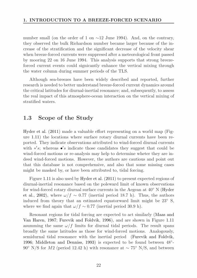
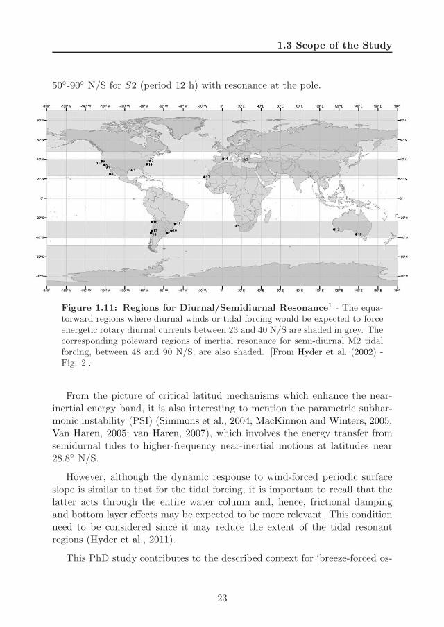
Hyder et al. (2011) made a valuable effort representing on a world map (Fig-ure 1.11) the locations where surface rotary diurnal currents have been re-ported. They indicate observations attributed to wind-forced diurnal currentswith ∗′s; whereas •′s indicate those candidates they suggest that could bewind-forced motions or re-analysis may help to determine wheter they are in-deed wind-forced motions. However, the authors are cautious and point outthat this database is not comprehensive, and also that some missing casesmight be masked by, or have been attributed to, tidal forcing.
Figure 1.11 is also used by Hyder et al. (2011) to present expected regions ofdiurnal-inertial resonance based on the poleward limit of known observationsfor wind-forced rotary diurnal surface currents in the Aegean at 40 N (Hyderet al., 2002), where ω/f ∼ 0.77 (inertial period 18.7 h). Thus, the authorsinduced from theory that an estimated equatorward limit might be 23 S,where we find again that ω/f ∼ 0.77 (inertial period 30.9 h).
Resonant regions for tidal forcing are expected to act similarly (Maas andVan Haren, 1987; Furevik and Foldvik, 1996), and are shown in Figure 1.11asumming the same ω/f limits for diurnal tidal periods. The result spansbroadly the same latitudes as those for wind-forced motions. Analogously,semidurnal tidal resonance with the inertial period (Furevik and Foldvik,1996; Middleton and Denniss, 1993) is expected to be found between 48-90 N/S for M2 (period 12.42 h) with resonance at ∼ 75 N/S, and between
22
1.3 Scope of the Study
50-90 N/S for S2 (period 12 h) with resonance at the pole.
Figure 1.11: Regions for Diurnal/Semidiurnal Resonance1 - The equa-torward regions where diurnal winds or tidal forcing would be expected to forceenergetic rotary diurnal currents between 23 and 40 N/S are shaded in grey. Thecorresponding poleward regions of inertial resonance for semi-diurnal M2 tidalforcing, between 48 and 90 N/S, are also shaded. [From Hyder et al. (2002) -Fig. 2].
From the picture of critical latitud mechanisms which enhance the near-inertial energy band, it is also interesting to mention the parametric subhar-monic instability (PSI) (Simmons et al., 2004; MacKinnon and Winters, 2005;Van Haren, 2005; van Haren, 2007), which involves the energy transfer fromsemidurnal tides to higher-frequency near-inertial motions at latitudes near28.8 N/S.
However, although the dynamic response to wind-forced periodic surfaceslope is similar to that for the tidal forcing, it is important to recall that thelatter acts through the entire water column and, hence, frictional dampingand bottom layer effects may be expected to be more relevant. This conditionneed to be considered since it may reduce the extent of the tidal resonantregions (Hyder et al., 2011).
This PhD study contributes to the described context for ‘breeze-forced os-
23

1. INTRODUCTION TO A BREEZE-FORCED SCENARIO
cillations’ providing observational results and analysis from four new locationson this topic around the Iberian Peninsula and hence framed poleward of thecritical latitude (30 N/S) for diurnal-inertial resonance.
Firstly, in Chapter 2 we use time series data from two regions which mayact as a proxy of resonant breeze-forced oscillations poleward of the criticallatitude for diurnal-inertial resonance: the Gulf of Cadiz and the Gulf ofValencia. Concurrently we also present time series data from a third region inwhich resonance is not expected to occurr. This last region is placed nearby,but out of the critical latitudes, and serves as a ‘blank test’ for our study: theCape Penas area. The research focused in this case on the characterization ofthe temporal evolution of observed breeze-forced oscillations. Special attentionis given to the effects of the phase correlation between the breeze forcing andthe subsequent ocean response giving rise to resonant breeze-forced oscillationsand, therefore, enhancing the diunal-inertial energy budget.
Secondly, in Chapter 3 we explore the role of breeze-forced-oscillations onpromoting diapycnal mixing processes. This research provides a new dataset of breeze-forced oscillations in the stratified waters of the Bay of Setubal,framed within the critical latitudes (30 ± 10 N/S) for diurnal-inertial reso-nance where they can greatly contribute to triggering diapycnal mixing.
24

Chapter 2
Breeze-Forced OscillationsPoleward of the CriticalLatitude for Diurnal-InertialResonance1
2.1 Outline
The present chapter focuses on the temporal evolution and variability ofbreeze-forced oscillations (BFOs) poleward of 30 N and near the limit fordiurnal-inertial resonance. Observations were collected from three differentregions around the Iberian Peninsula (from south to north): the Gulf of Cadizand the Gulf of Valencia (both regions being within the critical latitudes forresonance); and, the Cape Penas area (out of the critical latitudes for reso-nance). The time series data belong to the REDEXT (Red Exterior de Boyas)network of oceanographic and meteorological buoys, and were provided byPuertos del Estado (Spain).
Due to the rotary nature of the process, we find that rotary wavelet anal-ysis (Torrence and Compo, 1998; Hormazabal et al., 2002) is an obvious and
1Aguiar-Gonzalez B., Hormazabal S., Rodrıguez-Santana A., Cisneros-Aguirre J.,Martınez-Marrero. Breeze-Forced Oscillations around The Poleward Limit for Diurnal-Inertial Resonance. In Preparation to be Submitted to an International refereed Journal
25
2. BREEZE-FORCED OSC. AROUND THE POLEWARD LIMIT
suitable methodology to study the temporal evolution of breeze-forced oscil-lations. However, to our knowledge this is the first time that it is appliedwith this aim in the literature. Thus, we use rotary wavelet power spectrato characterize and quantify breeze-forced oscillation variance and variabilityaccording to its driving force, the sea-land breezes.
Additionally, we use rotary wavelet coherency and phase spectra to furtherexplore how breeze-forced oscillations arise and evolve in time according tothe onset of sea-land breezes; therefore, enhancing the diunal-inertial energybudget.
This research is based on time series data of surface current velocity andwind velocity over annual cycles from three REDEXT buoys. Data andmethodology are described in Section 3.2. In Section 3.3 we present anddiscuss the main results. Special attention is given to observed differencesbetween wind-forced diurnal-inertial oscillations within and out of the criticallatitudes for resonance. We summarize the main conclusions in Section 3.4.Appendix A describes the rotary wavelet method used in this study.
2.2 Data and Methodology
Time series data of surface current and wind velocity were provided by Puer-tos del Estado (Spain) from the REDEXT (Red Exterior de Boyas) networkof buoys. This network is composed of Wavescan and SeaWatch mooringsmeasuring oceanographic and meteorological variables all along the spanishcoastline. Locations of these moorings were originally chosen to be represen-tative of the surrounding ocean dynamics. Data are transmitted in real timevia satellite. After transmission, a control test is applied to guarantee qualityof measurements.
In this work we use REDEXT buoys from two different regions which mayact as a proxy of resonant breeze-forced oscillations poleward of 30 N andnear the limit for diurnal-inertial resonance: the Gulf of Cadiz and the Gulf ofValencia. The third region of study was intentionally selected nearby but outof the critical latitudes for diurnal-inertial resonance: the Cape Penas area.This configuration allow us to count with a ‘blank area’ in which resonance isnot expected to happen in comparison with other two areas where resonanceis expected. Thus, we can better elucidate how important can be a situationwhere resonant breeze-forced oscillations occurr as well as how different the
26
2.2 Data and Methodology
forced mechanism evolves in both situations. The locations of the three buoysare represented in Figure 2.1 and their corresponding inertial periods, offshoredistances and depths are listed in Table 2.1.
−5000
−5000
−5000
−500
0
−4000
−4000
−4000
−4000
−4000
−4000
−4000
−3000
−3000
−300
0
−3000
−3000−3000
−3000
−3000
−200
0
−2000
−200
0
−2000
−2000
−2000
−2000
−2000
−2000
−2000
−200
0−2000
−200
0
−2000
−200
0
−100
0
−100
0−1
000
−100
0
−100
0
−1000
−1000 −1000
−1000−1000
−1000
−100
0−1
000
−1000
−100
0
−70
0
−700
−700
−700
−700−700
−700
−700
−700
−700
−700
−700
−700
−700
−700
−700
−500
−500
−500
−500
−500
−500
−500−500−500
−500
−500
−500
−500
−500
−500
−500
−100
−100
−100
−100
−100
−100
−100
−100
−100 −100
−100
−100
−100
−100
−100
−100
Cape Peñas (2242)
Bay of Setúbal (Chapter 3 in This Work)
Gulf of Cádiz (2342)
Valencia II (2630)
12oW 9oW 6oW 3oW 0o 3oE
36oN
38oN
40oN
42oN
44oN
Longitude
Latit
ude
Figure 2.1: Oceanographic Buoys - Puertos del Estado - Map of theIberian Peninsula showing the oceanographic buoys used in this study and pro-vided by Puertos del Estado from the REDEXT network (Red Exterior de Boyas).Isobath of 200 m is highlighted in grey (thick line).
In the Gulf of Cadiz, Gulf of Valencia and Cape Penas area, time seriesof surface current velocity are collected from UCM-60 current meters settledin Seawatch REDEXT buoys, which have been providing oceanographic andmeteorological data since August 1996, September 2005 and March 1998, re-spectively. The current meter measures velocity at 3 m depth (range: 0 to3 m s−1 1% accuracy and current direction within ± 1). Meteorological sen-sors (Aandera 2740 and Aandera 3590) measure wind velocity (up to 70 m s−1)and direction at 3 m over the surface with an accuracy of 1.5% and 1%, re-spectively (Criado-Aldeanueva et al., 2009). Both surface current and wind
27
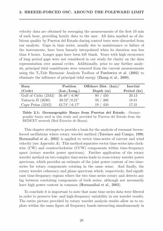
2. BREEZE-FORCED OSC. AROUND THE POLEWARD LIMIT
velocity data are obtained by averaging the measurements of the first 10 minof each hour, providing hourly data to the user. All data marked as of du-bitous quality by Puertos del Estado during control tests were discarded fromour analysis. Gaps in time series, usually due to maintenance or failure ofthe instruments, have been linearly interpolated when its duration was lessthan 8 hours. Longer gaps have been left blank. Years with high recurrenceof long period gaps were not considered in our study for clarity on the datarepresentation over annual cycles. Additionally, prior to any further analy-sis, principal tidal constituents were removed from the current measurementsusing the T Tide Harmonic Analysis Toolbox of Pawlowicz et al. (2002) toeliminate the influence of principal tidal energy (Zhang et al., 2009).
Buoy Position Offshore Dist. (km)/ Inertial
(Code) (Lat./Long.) Depth (m) Period (hr)
Gulf of Cadiz (2342) 36.48/-6.96 80 / 450 20.13Valencia II (2630) 39.52/0.21 59 / 260 18.81Cape Penas (2242) 43.74/-6.17 19 / 450 17.31
Table 2.1: Oceanographic Buoys from Puertos del Estado - Oceano-graphic buoys used in this study and provided by Puertos del Estado from theREDEXT network (Red Exterior de Boyas).
This chapter attempts to provide a basis for the analysis of resonant breeze-forced oscillations where rotary wavelet method (Torrence and Compo, 1998;Hormazabal et al., 2002) is applied to vector time-series of current and windvelocity (see Appendix A). This method separates vector time-series into clock-wise (CW) and counterclockwise (CCW) components within time-frequencyspace (rotary wavelet power spectrum). Further application of the rotarywavelet method on two complex time-series leads to cross-rotary wavelet powerspectrum, which provides an estimate of the joint power content of two time-series for rotary components rotating in the same sense. And finally, therotary wavelet coherency and phase spectrum which, respectively, find signifi-cant time-frequency regions where the two time series covary and detects anylag between corotating components of both series, although not necessarilyhave high power content in common (Hormazabal et al., 2002).
To conclude it is important to note that none time series data were filteredin order to preserve low- and high-frequency variability in our wavelet results.The entire picture provided by rotary wavelet analysis results allow us to ex-plore within the same figure all frequency bands interacting simultaneously in
28
2.3 Results and Discussion
time and frequency domains for both the atmosphere and the ocean. However,characterization of the general atmosphere/ocean circulation in the areas ofstudy is beyond the scope of this research1 and, hence, dominant long-periodprocesses will be addressed here only when they play a role on the dynamicsof the analyzed breeze-forced scenario.
2.3 Results and Discussion
2.3.1 Characterization of Three Wind-Forced Scenarios
We present a wavelet rotary analysis of meteorological and oceanographictime series data from three different regions around the Iberian Peninsula tocharacterize the temporal evolution adn variability of sea-land breezes and theocean response to this wind forcing.
Hence, we explore qualitatively simultaneous and co-located measurementsof wind at 3 m above the sea surface and ocean currents at 3 m depth. In thenext section we use the rotary wavelet method to quantify current variancein response to breeze forcing as well as to investigate the effects of the phasecorrelation between the forcing and the ocean response in the enhancement ofbreeze-forced oscillations.
Geographically, the Gulf of Cadiz and the Gulf of Valencia are framedwithin the critical latitudes for diurnal-inertial resonance (30 ± 10 N/S).The Cape Penas area bounds the poleward limit though being out of thisrange of latitudes (Figure 2.1; see also Table 2.1 for details on local inertialperiods). The three areas present a wide continental shelf for the developmentof the coastal breeze-forced oscillations subject of this study.
A) Temporal Evolution of Sea-land Breezes
Sea-land breezes are thermally-induced winds and so their strength is di-rectly proportional to the temperature gradient between air over land and airover the ocean (Pielke and Segal, 1986). Consequently, one may expect tofind higher recurrence and intensity of sea-land breeze events during periods
1Details on the main currents and tidal components for REDEXT buoys can be foundin http://www.puertos.es.
29
2. BREEZE-FORCED OSC. AROUND THE POLEWARD LIMIT
of strong daytime heating and night time cooling in the absence of large scalewind systems.
These conditions can be found specially during summer months when largesea-land temperature differences are accompanied by favourable synoptic con-ditions and sea-land breezes do not need to overcome winds from differentdirections driven by the passage of cyclones and anticyclones.
On the contrary, during winter months breezes need a larger temperaturedifference between land and sea than in summer to promote breezes gettingover large scale wind systems1. As a consequence, sea-land breezes are lessprobable to occur under this scenario. Spring and autumn months representthe transitional periods between both situations.
Figures 2.2-2.4 show the rotary wavelet power spectra of wind at the buoyslocated in the Gulf of Cadiz, the Gulf of Valencia and the Cape Penas area,respectively.
Firstly, in Figure 2.2, we observe that the temporal evolution of the windvariance at the Gulf of Cadiz shows a clear seasonal pattern within the diurnalband, the weather band (2-8 days) and the intraseasonal band (16-64 days),for both the clockwise and counterclockwise senses.
The diurnal wind variance appears as a well-defined packet which is vis-ibly enhanced from the early spring to the early autumn (April-October) incomparison to the lately autumn and winter months (November-March). Onthe contrary, the weather band and the intraseasonal band involve broaderphenomena in the frequency domain and are specially enhanced during wintermonths, when large scale wind systems are more active. The weakening ofthese low-frequency bands occur from the early spring to the early autumn,what greatly benefits the onset and enhacement of sea land breezes which donot have to overcome winds from large scale scale systems.
1It has been tested with time series data of atmospheric pressure (not shown here) fromthe three REDEXT buoys that the three areas of study present regularly calm weatherconditions during summer months and a more intense large scale activity during wintermonths.
30
2.3 Results and Discussion
Figure 2.2: Rotary Wavelet Power Spectrum of Wind at the BuoyGulf of Cadiz - Rotary wavelet power spectrum of surface winds (3 m abovesea surface) measured at the Buoy Gulf of Cadiz. (upper pannel) Total rotarywavelet power spectrum. (intermediate pannel) Rotary wavelet power spectrumof clockwise component. (lower pannel) Rotary wavelet power spectrum of coun-terclockwise component. The two black lines on either end indicate the ‘cone ofinfluence’ where edge effects become important.
The pattern described above is consistent with that indicated for the cli-matology of a sea-land breeze system (Hunter et al., 2007; Zhang et al., 2009).The diurnal wind variance observed during nonsummer seasons may be forcedby mechanisms other than sea-land breezes, such as synoptic wind events. Thesame cause has been pointed out for diurnal wind variance observed duringnon-breezes periods on the Texas-Lousiana shelf (Chen et al., 1996; Zhanget al., 2009). For this reason in Section 2.3.2 we will use only data fromspring-summer months for our analysis on the effects of the phase correlationbetween the breeze forcing and the subsequent ocean response giving rise toresonant breeze-forced oscillations.
31
2. BREEZE-FORCED OSC. AROUND THE POLEWARD LIMIT
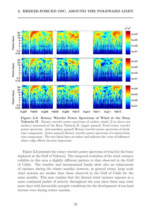
Figure 2.3: Rotary Wavelet Power Spectrum of Wind at the BuoyValencia II - Rotary wavelet power spectrum of surface winds (3 m above seasurface) measured at the Buoy Valencia II. (upper pannel) Total rotary waveletpower spectrum. (intermediate pannel) Rotary wavelet power spectrum of clock-wise component. (lower pannel) Rotary wavelet power spectrum of counterclock-wise component. The two black lines on either end indicate the ‘cone of influence’where edge effects become important.
Figure 2.3 presents the rotary wavelet power spectrum of wind for the buoydeployed at the Gulf of Valencia. The temporal evolution of the wind varianceexhibits in this area a slightly different pattern to that observed in the Gulfof Cadiz. The weather and intraseasonal bands show also an enhacementof variance during the winter months; however, in general terms, large scalewind systems are weaker than those observed in the Gulf of Cadiz for thesame months. This may explain that the diurnal wind variance appears as amore continued packet of activity throughout the year since there may existmore days with favourable synoptic conditions for the development of sea-landbreezes even during winter months.
32
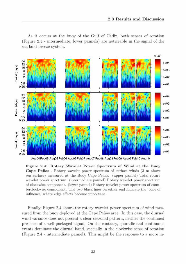
2.3 Results and Discussion
As it occurs at the buoy of the Gulf of Cadiz, both senses of rotation(Figure 2.3 - intermediate, lower pannels) are noticeable in the signal of thesea-land breeze system.
Figure 2.4: Rotary Wavelet Power Spectrum of Wind at the BuoyCape Penas - Rotary wavelet power spectrum of surface winds (3 m abovesea surface) measured at the Buoy Cape Penas. (upper pannel) Total rotarywavelet power spectrum. (intermediate pannel) Rotary wavelet power spectrumof clockwise component. (lower pannel) Rotary wavelet power spectrum of coun-terclockwise component. The two black lines on either end indicate the ‘cone ofinfluence’ where edge effects become important.
Finally, Figure 2.4 shows the rotary wavelet power spectrum of wind mea-sured from the buoy deployed at the Cape Penas area. In this case, the diurnalwind variance does not present a clear seasonal pattern, neither the continuedpresence of a well-packaged signal. On the contrary, sporadic and continuousevents dominate the diurnal band, specially in the clockwise sense of rotation(Figure 2.4 - intermediate pannel). This might be the response to a more in-
33
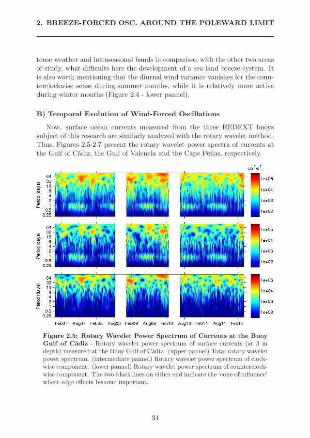
2. BREEZE-FORCED OSC. AROUND THE POLEWARD LIMIT
tense weather and intraseasonal bands in comparison with the other two areasof study, what difficults here the development of a sea-land breeze system. Itis also worth mentioning that the diurnal wind variance vanishes for the coun-terclockwise sense during summer months, while it is relatively more activeduring winter months (Figure 2.4 - lower pannel).
B) Temporal Evolution of Wind-Forced Oscillations
Now, surface ocean currents measured from the three REDEXT buoyssubject of this research are similarly analyzed with the rotary wavelet method.Thus, Figures 2.5-2.7 present the rotary wavelet power spectra of currents atthe Gulf of Cadiz, the Gulf of Valencia and the Cape Penas, respectively.
Figure 2.5: Rotary Wavelet Power Spectrum of Currents at the BuoyGulf of Cadiz - Rotary wavelet power spectrum of surface currents (at 3 mdepth) measured at the Buoy Gulf of Cadiz. (upper pannel) Total rotary waveletpower spectrum. (intermediate pannel) Rotary wavelet power spectrum of clock-wise component. (lower pannel) Rotary wavelet power spectrum of counterclock-wise component. The two black lines on either end indicate the ‘cone of influence’where edge effects become important.
34
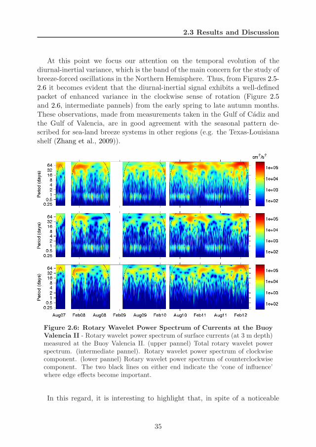
2.3 Results and Discussion
At this point we focus our attention on the temporal evolution of thediurnal-inertial variance, which is the band of the main concern for the study ofbreeze-forced oscillations in the Northern Hemisphere. Thus, from Figures 2.5-2.6 it becomes evident that the diurnal-inertial signal exhibits a well-definedpacket of enhanced variance in the clockwise sense of rotation (Figure 2.5and 2.6, intermediate pannels) from the early spring to late autumn months.These observations, made from measurements taken in the Gulf of Cadiz andthe Gulf of Valencia, are in good agreement with the seasonal pattern de-scribed for sea-land breeze systems in other regions (e.g. the Texas-Louisianashelf (Zhang et al., 2009)).
Figure 2.6: Rotary Wavelet Power Spectrum of Currents at the BuoyValencia II - Rotary wavelet power spectrum of surface currents (at 3 m depth)measured at the Buoy Valencia II. (upper pannel) Total rotary wavelet powerspectrum. (intermediate pannel). Rotary wavelet power spectrum of clockwisecomponent. (lower pannel) Rotary wavelet power spectrum of counterclockwisecomponent. The two black lines on either end indicate the ‘cone of influence’where edge effects become important.
In this regard, it is interesting to highlight that, in spite of a noticeable
35

2. BREEZE-FORCED OSC. AROUND THE POLEWARD LIMIT
signal of diurnal wind forcing all along the year in the Gulf of Valencia (Fig-ure 2.3), breeze-forced oscillation variance is enchanced only from the earlyspring to the late autumn months (Figure 2.6 - intermediate pannel). Thisscenario responds to previous description given in Chapter 1, where the verti-cal structure of breeze-forced oscillations was shown to be partially supportedby a first baroclinic mode marked by the depth of the pycnocline in stratifiedwaters (Simpson et al., 2002; Rippeth et al., 2002; Zhang et al., 2009; Hyderet al., 2011). This explains that during winter months in the Gulf of Valencia,even in presence of breeze-forcing, the ocean response does not develop aneffective transfer of momentum from wind to the interior of the water column.
Figure 2.7: Rotary Wavelet Power Spectrum of Currents at the BuoyCape Penas - Rotary wavelet power spectrum of surface currents (at 3 m depth)measured at the Buoy Cape Penas. (upper pannel) Total rotary wavelet powerspectrum. (intermediate pannel) Rotary wavelet power spectrum of clockwisecomponent. (lower pannel) Rotary wavelet power spectrum of counterclockwisecomponent. The two black lines on either end indicate the ‘cone of influence’where edge effects become important.
The previous two areas of study, the Guf of Cadiz and the Gulf of Valen-
36
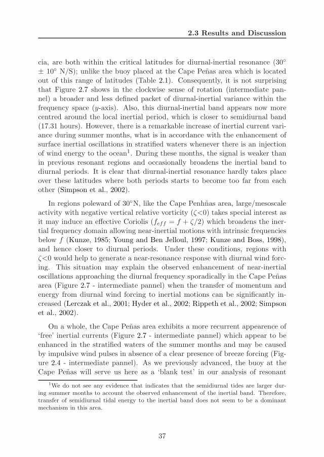
2.3 Results and Discussion
cia, are both within the critical latitudes for diurnal-inertial resonance (30
± 10 N/S); unlike the buoy placed at the Cape Penas area which is locatedout of this range of latitudes (Table 2.1). Consequently, it is not surprisingthat Figure 2.7 shows in the clockwise sense of rotation (intermediate pan-nel) a broader and less defined packet of diurnal-inertial variance within thefrequency space (y-axis). Also, this diurnal-inertial band appears now morecentred around the local inertial period, which is closer to semidiurnal band(17.31 hours). However, there is a remarkable increase of inertial current vari-ance during summer months, what is in accordance with the enhancement ofsurface inertial oscillations in stratified waters whenever there is an injectionof wind energy to the ocean1. During these months, the signal is weaker thanin previous resonant regions and occasionally broadens the inertial band todiurnal periods. It is clear that diurnal-inertial resonance hardly takes placeover these latitudes where both periods starts to become too far from eachother (Simpson et al., 2002).
In regions poleward of 30N, like the Cape Penhnas area, large/mesoscaleactivity with negative vertical relative vorticity (ζ<0) takes special interest asit may induce an effective Coriolis (feff = f + ζ/2) which broadens the iner-tial frequency domain allowing near-inertial motions with intrinsic frequenciesbelow f (Kunze, 1985; Young and Ben Jelloul, 1997; Kunze and Boss, 1998),and hence closer to diurnal periods. Under these conditions, regions withζ<0 would help to generate a near-resonance response with diurnal wind forc-ing. This situation may explain the observed enhancement of near-inertialoscillations approaching the diurnal frequency sporadically in the Cape Penasarea (Figure 2.7 - intermediate pannel) when the transfer of momentum andenergy from diurnal wind forcing to inertial motions can be significantly in-creased (Lerczak et al., 2001; Hyder et al., 2002; Rippeth et al., 2002; Simpsonet al., 2002).
On a whole, the Cape Penas area exhibits a more recurrent appearence of‘free’ inertial currents (Figure 2.7 - intermediate pannel) which appear to beenhanced in the stratified waters of the summer months and may be causedby impulsive wind pulses in absence of a clear presence of breeze forcing (Fig-ure 2.4 - intermediate pannel). As we previously advanced, the buoy at theCape Penas will serve us here as a ‘blank test’ in our analysis of resonant
1We do not see any evidence that indicates that the semidiurnal tides are larger dur-ing summer months to account the observed enhancement of the inertial band. Therefore,transfer of semidiurnal tidal energy to the inertial band does not seem to be a dominantmechanism in this area.
37
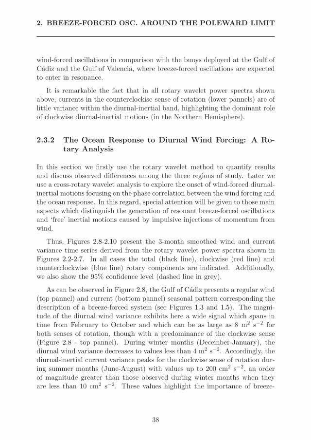
2. BREEZE-FORCED OSC. AROUND THE POLEWARD LIMIT
wind-forced oscillations in comparison with the buoys deployed at the Gulf ofCadiz and the Gulf of Valencia, where breeze-forced oscillations are expectedto enter in resonance.
It is remarkable the fact that in all rotary wavelet power spectra shownabove, currents in the counterclockise sense of rotation (lower pannels) are oflittle variance within the diurnal-inertial band, highlighting the dominant roleof clockwise diurnal-inertial motions (in the Northern Hemisphere).
2.3.2 The Ocean Response to Diurnal Wind Forcing: A Ro-tary Analysis
In this section we firstly use the rotary wavelet method to quantify resultsand discuss observed differences among the three regions of study. Later weuse a cross-rotary wavelet analysis to explore the onset of wind-forced diurnal-inertial motions focusing on the phase correlation between the wind forcing andthe ocean response. In this regard, special attention will be given to those mainaspects which distinguish the generation of resonant breeze-forced oscillationsand ‘free’ inertial motions caused by impulsive injections of momentum fromwind.
Thus, Figures 2.8-2.10 present the 3-month smoothed wind and currentvariance time series derived from the rotary wavelet power spectra shown inFigures 2.2-2.7. In all cases the total (black line), clockwise (red line) andcounterclockwise (blue line) rotary components are indicated. Additionally,we also show the 95% confidence level (dashed line in grey).
As can be observed in Figure 2.8, the Gulf of Cadiz presents a regular wind(top pannel) and current (bottom pannel) seasonal pattern corresponding thedescription of a breeze-forced system (see Figures 1.3 and 1.5). The magni-tude of the diurnal wind variance exhibits here a wide signal which spans intime from February to October and which can be as large as 8 m2 s−2 forboth senses of rotation, though with a predominance of the clockwise sense(Figure 2.8 - top pannel). During winter months (December-January), thediurnal wind variance decreases to values less than 4 m2 s−2. Accordingly, thediurnal-inertial current variance peaks for the clockwise sense of rotation dur-ing summer months (June-August) with values up to 200 cm2 s−2, an orderof magnitude greater than those observed during winter months when theyare less than 10 cm2 s−2. These values highlight the importance of breeze-
38
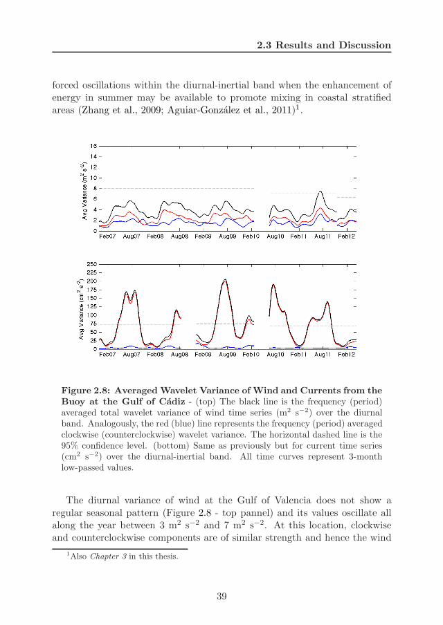
2.3 Results and Discussion
forced oscillations within the diurnal-inertial band when the enhancement ofenergy in summer may be available to promote mixing in coastal stratifiedareas (Zhang et al., 2009; Aguiar-Gonzalez et al., 2011)1.
Figure 2.8: Averaged Wavelet Variance of Wind and Currents from theBuoy at the Gulf of Cadiz - (top) The black line is the frequency (period)averaged total wavelet variance of wind time series (m2 s−2) over the diurnalband. Analogously, the red (blue) line represents the frequency (period) averagedclockwise (counterclockwise) wavelet variance. The horizontal dashed line is the95% confidence level. (bottom) Same as previously but for current time series(cm2 s−2) over the diurnal-inertial band. All time curves represent 3-monthlow-passed values.
The diurnal variance of wind at the Gulf of Valencia does not show aregular seasonal pattern (Figure 2.8 - top pannel) and its values oscillate allalong the year between 3 m2 s−2 and 7 m2 s−2. At this location, clockwiseand counterclockwise components are of similar strength and hence the wind
1Also Chapter 3 in this thesis.
39
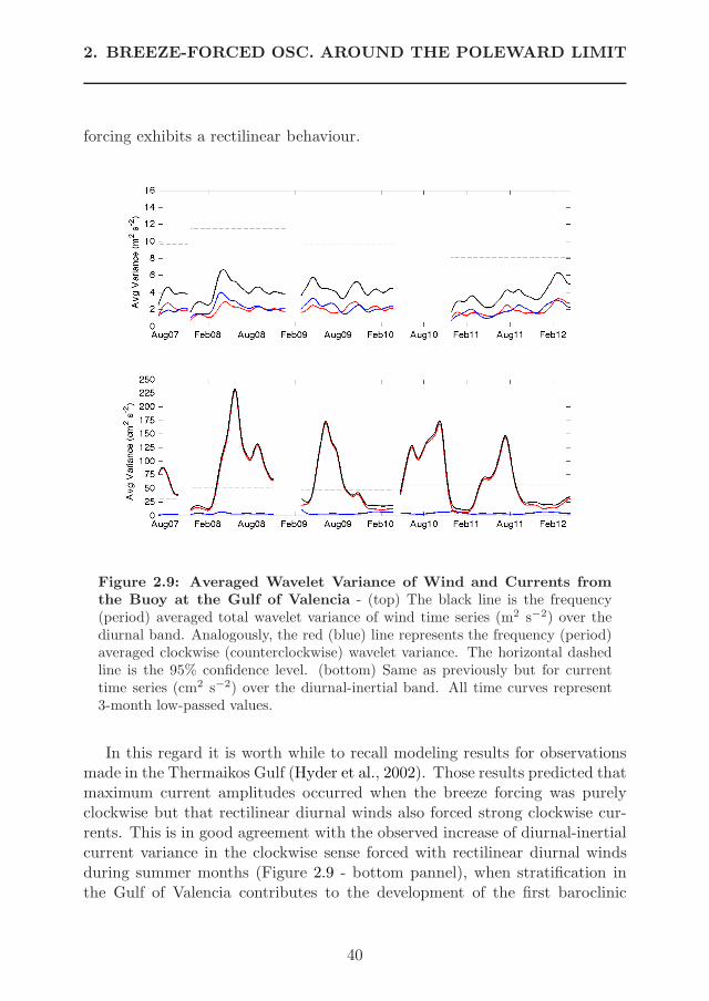
2. BREEZE-FORCED OSC. AROUND THE POLEWARD LIMIT
forcing exhibits a rectilinear behaviour.
Figure 2.9: Averaged Wavelet Variance of Wind and Currents fromthe Buoy at the Gulf of Valencia - (top) The black line is the frequency(period) averaged total wavelet variance of wind time series (m2 s−2) over thediurnal band. Analogously, the red (blue) line represents the frequency (period)averaged clockwise (counterclockwise) wavelet variance. The horizontal dashedline is the 95% confidence level. (bottom) Same as previously but for currenttime series (cm2 s−2) over the diurnal-inertial band. All time curves represent3-month low-passed values.
In this regard it is worth while to recall modeling results for observationsmade in the Thermaikos Gulf (Hyder et al., 2002). Those results predicted thatmaximum current amplitudes occurred when the breeze forcing was purelyclockwise but that rectilinear diurnal winds also forced strong clockwise cur-rents. This is in good agreement with the observed increase of diurnal-inertialcurrent variance in the clockwise sense forced with rectilinear diurnal windsduring summer months (Figure 2.9 - bottom pannel), when stratification inthe Gulf of Valencia contributes to the development of the first baroclinic
40
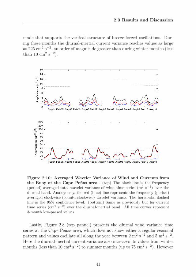
2.3 Results and Discussion
mode that supports the vertical structure of breeze-forced oscillations. Dur-ing these months the diurnal-inertial current variance reaches values as largeas 225 cm2 s−2, an order of magnitude greater than during winter months (lessthan 10 cm2 s−2).
Figure 2.10: Averaged Wavelet Variance of Wind and Currents fromthe Buoy at the Cape Penas area - (top) The black line is the frequency(period) averaged total wavelet variance of wind time series (m2 s−2) over thediurnal band. Analogously, the red (blue) line represents the frequency (period)averaged clockwise (counterclockwise) wavelet variance. The horizontal dashedline is the 95% confidence level. (bottom) Same as previously but for currenttime series (cm2 s−2) over the diurnal-inertial band. All time curves represent3-month low-passed values.
Lastly, Figure 2.8 (top pannel) presents the diurnal wind variance timeseries at the Cape Penas area, which does not show either a regular seasonalpattern and values oscillate all along the year between 2 m2 s−2 and 5 m2 s−2.Here the diurnal-inertial current variance also increases its values from wintermonths (less than 10 cm2 s−2) to summer months (up to 75 cm2 s−2). However
41

2. BREEZE-FORCED OSC. AROUND THE POLEWARD LIMIT
it is clear that the enhacenment of the inertial variance is not as large as inthe Gulf of Cadiz and the Gulf of Valencia, where resonance between diurnalwind forcing and inertial motions from the ocean response may occur.
After quantifying observed differences between resonant breeze-forced os-cillations within critical latitudes and wind-forced inertial oscillations out ofthis range of latitudes, now we proceed to explore the wavelet coherency andphase spectra between wind and currents to characterize the onset of bothtypes of inertial motions.
With this aim, we use two time series data (of two months each one) cor-responding to spring-summer periods as representative of a situation in whichboth resonant breeze-forced oscillations in the Gulf of Cadiz and wind-forcedinertial oscillations in the Cape Penas area are present1.
Thus Figures 2.11 and 2.12 show the wavelet coherency and phase spec-tra between wind and current clockwise components, which are of the mainconcern for the study of diurnal-inertial motions in the Northern Hemisphere.The top and intermediate pannels present rotary wavelet power spectrum ofwind and currents (clockwise componsents), respectively, in order to accountthe diurnal-inertial variance in relation with the wavelet coherency and phasespectra between wind and currents. The red color in the squared wavelet co-herency spectra (bottom pannel) means that coherency (γ2) is high, while theblue means it is low. The vectors indicate the phase difference between windand current at different frequencies and at each time (bottom pannel). Forclarity only one vector is plotted for each day. Positive phase angles betweenwind and current indicate that current leads wind. Accordingly, vectors are inphase pointing straight up, out of phase pointing straight down, and currentleads wind by 90 pointing right. Only phase angles (vectors) for γ2 > 0.7 areplotted.
As can be observed in Figure 2.11 (Gulf of Cadiz), the wind and currentshow high coherency (γ2 >0.7) in the diurnal-inertial band for most of April-May 2007 with large associated diurnal-inertial current variance. These resultssupport that the near-resonant condition in this area promotes the generation
1Time series data from the Gulf of Valencia exhibit an analogous pattern (not shownhere) to that described for the onset of resonant breeze-forced oscillations during spring-summer months in the Gulf of Cadiz and, hence, we assume the latter may be representativeof the onset of resonant BFOs poleward of the critical latitude for diurnal-inertial resonance(30 N/S).
42
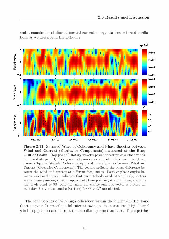
2.3 Results and Discussion
and accumulation of diurnal-inertial current energy via breeze-forced oscilla-tions as we describe in the following.
Figure 2.11: Squared Wavelet Coherency and Phase Spectra betweenWind and Current (Clockwise Components) measured at the BuoyGulf of Cadiz - (top pannel) Rotary wavelet power spectrum of surface winds.(intermediate pannel) Rotary wavelet power spectrum of surface currents. (lowerpannel) Squared Wavelet Coherency (γ2) and Phase Spectra between Wind andCurrent (Clockwise Components). The vectors indicate the phase difference be-tween the wind and current at different frequencies. Positive phase angles be-tween wind and current indicates that current leads wind. Accordingly, vectorsare in phase pointing straight up, out of phase pointing straight down, and cur-rent leads wind by 90 pointing right. For clarity only one vector is plotted foreach day. Only phase angles (vectors) for γ2 > 0.7 are plotted.
The four patches of very high coherency within the diurnal-inertial band(bottom pannel) are of special interest owing to its associated high diurnalwind (top pannel) and current (intermediate pannel) variance. These patches
43
2. BREEZE-FORCED OSC. AROUND THE POLEWARD LIMIT
are representative of breeze-forced events and are observed during 8-13 April,19-23 April, 28 April - 2 May and 3-17 May. All these events start with thesame pattern, diurnal wind (breezes) variance arises preceding the increase ofdiurnal-inertial current variance (breeze-forced oscillations), which is in phasewith vectors pointing straight up.
At times after the onset of the phenomenon, the phase difference betweenwind forcing and forced-currents slightly increases to positive phase angles(vectors deviate pointing to the right), and therefore currents leads wind forc-ing. This pattern may be consistent with an alternation of cycles of forcedoscillations, when current motions are in phase with wind forcing, and cyclesof decreased forcing when the currents tend to revert to ‘free’ inertial oscilla-tions (Simpson et al., 2002). This would explain that in Figure 2.11, wheneverthe forcing decreases, the observed phase difference between wind and currentsincreases and tends to show inertial current phase leading diurnal wind phasesince at latitudes poleward of 30 N/S ‘free’ inertial motions are of higherfrequency than diurnal motions.
If the wind forcing vanishes completely after several days being active, thesituation could be similar to that observed for the breeze-forced event startingon 3 May (Figure 2.11 - bottom pannel). After more than 10 days of constantwind forcing, diurnal wind variance drops on 17 May; however diurnal-inertialcurrent variance is still high and from then ‘free’ inertial oscillations dominate(see in intermediate pannel the decreasing tendency from diurnal to inertialperiod). As expected, low coherency values between wind and currents arefound for days after 17 May, when the breeze forcing has disappeared (toppannel).
The enhancement of diurnal-inertial current variance observed in Figure 2.11,and related to a high coherency between forcing and forced-motions, suggeststhat energetic breeze-forced events are promoted when the relationship be-tween wind and currents lasts for several cycles. These results are in goodagreement with previous observations reported by Zhang et al. (2009) on theTexas-Louisiana shelf (equatorward of 30 N). They suggested that the longerthis in phase relationship persists, the larger the magnitude of the diurnal-inertial current becomes until a steady state is reached.
44
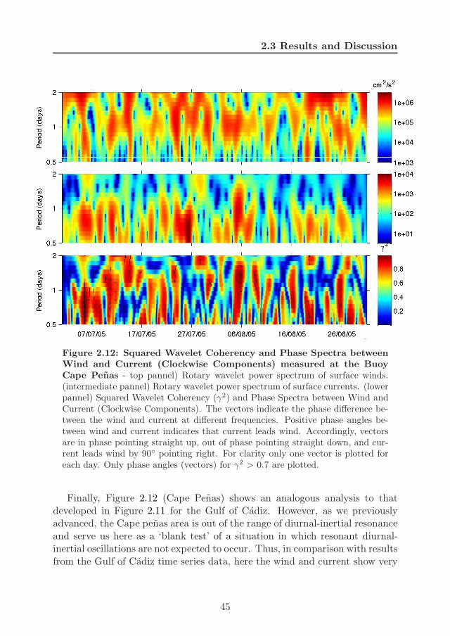
2.3 Results and Discussion
Figure 2.12: Squared Wavelet Coherency and Phase Spectra betweenWind and Current (Clockwise Components) measured at the BuoyCape Penas - top pannel) Rotary wavelet power spectrum of surface winds.(intermediate pannel) Rotary wavelet power spectrum of surface currents. (lowerpannel) Squared Wavelet Coherency (γ2) and Phase Spectra between Wind andCurrent (Clockwise Components). The vectors indicate the phase difference be-tween the wind and current at different frequencies. Positive phase angles be-tween wind and current indicates that current leads wind. Accordingly, vectorsare in phase pointing straight up, out of phase pointing straight down, and cur-rent leads wind by 90 pointing right. For clarity only one vector is plotted foreach day. Only phase angles (vectors) for γ2 > 0.7 are plotted.
Finally, Figure 2.12 (Cape Penas) shows an analogous analysis to thatdeveloped in Figure 2.11 for the Gulf of Cadiz. However, as we previouslyadvanced, the Cape penas area is out of the range of diurnal-inertial resonanceand serve us here as a ‘blank test’ of a situation in which resonant diurnal-inertial oscillations are not expected to occur. Thus, in comparison with resultsfrom the Gulf of Cadiz time series data, here the wind and current show very
45
2. BREEZE-FORCED OSC. AROUND THE POLEWARD LIMIT
low coherency and the diurnal-inertial phase difference (bottom pannel) ishighly variable for most of the analysed period (July-August 2005)1. It isclear that there exists diurnal wind forcing acting during this period (toppannel); however, there is no evidence of this wind forces periodic diurnal-inertial currents. The inertial current variance (intermediate pannel) seems torespond to impulsive injections of momentum from diurnal wind (top pannel)although beyond that initial pulse, near-inertial currents may oscillate ‘freely’.Therefore, the dominant ocean response appears to be in the form of transientoscillations which do not accumulate efficiently near-inertial energy in time asit occurs in regions of diurnal-inertial resonance where forced currents maylast for several cycles.
2.4 Conclusions
We use time series data of surface current velocity and wind velocity overannual cycles from three different regions around the Iberian Peninsula: theGulf of Cadiz and the Gulf of Valencia (both regions within the critical lati-tudes for resonance); and, the Cape Penas area (out of the critical latitudesfor resonance).
Rotary wavelet analysis results provide evidence that sea-land breeze forc-ing enhances clockwise rotary current motions (breeze-forced oscillations) whichgreatly contribute to near-inertial energy budget and its variability in the Gulfof Cadiz and the Gulf of Valencia (Northern Hemisphere). These results alsosupport that the near-resonant condition in these areas promotes the gen-eration and accumulation of diurnal-inertial current energy via breeze-forcedoscillations. Squared wavelet coherency and phase spectra suggest that ener-getic breeze-forced events are enhanced when the relationship between windand currents lasts for several cycles and present a high coherency between theforcing and forced-motions being in phase.
We find that the diurnal-inertial current variance attributed to breeze-forced oscillations exhibits a clear seasonal pattern which peaks during spring-summer months, presumably due to observed strong breeze events take place
1This analysis has been performed with other periods of time in the area of study andanalogous results were found.
46

2.4 Conclusions
when coastal waters are sufficiently stratified1. This enhancement of diurnal-inertial current variance due to breeze-forced oscillations in the Gulf of Cadizand the Gulf of Valencia has been estimated to be as large as on order of mag-nitude higher during summer months (reaching values of up to 225 cm2 s−2)than in winter months (values are less than 10 cm2 s−2).
Despite the fact that this research focuses on time series data from the Gulfof Cadiz and the Gulf of Valencia, we find that these results and methodologymay have applications to the study of breeze-forced oscillations over othercoastal areas poleward of the critical latitude for diurnal-inertial resonance(30N/S).
The inertial current variance in the Cape Penas area also exhibits a seasonalpattern and increases its values from winter months (less than 10 cm2 s−2)to summer months (up to 75 cm2 s−2). However, this enhacenment is not aslarge as in the Gulf of Cadiz and the Gulf of Valencia, where resonance betweendiurnal wind forcing and inertial motions from the ocean response may occur.The inertial current variance in the Cape Penas area seems to respond toimpulsive injections of momentum from diurnal wind. The dominant oceanresponse appears to be in the form of transient ‘free’ oscillations which do notefficiently accumulate near-inertial energy in time as it occurs in regions ofdiurnal-inertial resonance where forced currents may last for several cycles.
These results support the role of resonant breeze-forced oscillations on thegeneration and accumulation of near-inertial energy which may be available forpromoting vertical mixing with important consequences on coastal dynamicsas we will explore in the following chapter.
1We explore the effects of breeze-forced oscillations in stratified waters, and associateddiapycnal mixing proccess, in Chapter 3.
47

2. BREEZE-FORCED OSC. AROUND THE POLEWARD LIMIT
48

Chapter 3
Breeze-Forced Oscillationsand Diapycnal Mixing1
3.1 Outline
This chapter presents an analysis of diapycnal mixing processes triggered bybreeze-forced oscillations (BFOs) with observational data. Our interest fo-cused on the relative importance of this phenomenon overcoming the verticalstability of the water column. The goal is to highlight breeze-forced oscillationdynamics in areas where the coast exhibits a well-developed sea-land breezeregime; and, hence, the ocean response is strongly controlled by breeze-forceddynamics. Our research is based on previous literature and new observationsof BFOs taken during the Maritime Rapid Environmental Assessment 2004(MREA04) sea trial off the west coast of the Iberian Peninsula, within thecritical latitudes for diurnal-inertial resonance. Additionally, we also countwith wind data from a meteorological land station provided by the InstitutoHidrografico - Portugal
Analysis of the measurements shows evidence of dominant circular anticy-clonic oscillations forced by sea-land breezes acting during the MREA exerciseinto the Bay of Setubal (Portugal). Furthermore, currents were distributed
1Aguiar-Gonzalez B., Rodrıguez-Santana A., Cisneros-Aguirre J., Martınez-Marrero.2011. Diurnal-inertial motions and diapycnal mixing on the Portuguese shelf. Cont. Shelf.
Res. 31, 1193–1201.
49
3. BREEZE-FORCED OSC. AND DIAPYCNAL MIXING
into two main layers with highly stratified and vertically sheared flows. Surfacestratification entered into the system through the Sado Estuary (freshwaterinput). As it will be discussed, breeze-forced currents were found to promotemixing in stratified shallow waters of the shelf area over the scale of a fewdays. The period of observation counts with days of breeze and relaxed-windevents, what allowed us to track the evolution of the water column at differentstages.
Wind conditions were determined with an Aanderaa meteorological buoyplaced in the Bay of Setubal during the MREA04 experiment. Currents datawere recorded from two Barny ADCP (Acoustic Doppler Current Profiler)deployments located on the north and south sides of the bay, respectively.Both ADCP’s covered almost the full depth of water (∼ 112 m) with 24 binsof 4 m size at both sites. Simultaneous CTD (Conductivity, Temperature,Depth) and data were used to analyse the strength of observed breeze-forcedoscillations in promoting diapycnal mixing through the squared vertical shear(S2), squared buoyancy frequency (N2) and gradient Richardson Number (Ri)of the water column.
The potential role that breeze-forced oscillations may play in shelf areaswith low tidal energy has been recurrently highlighted in the literature. Ver-tically sheared flows in stratified waters may lead to diapycnal mixing and,correspondingly, one could expect that breeze-forced oscillations in stratifiedwaters may promote mixing throghout the water column. Nevertheless, to thebest of our knowledge only one paper previous to this study (Zhang et al.,2009) has addressed an analysis which explicitely supports observational evi-dence of this role.
The present research provides a new data set of breeze-forced oscillations instratified waters near the critical latitudes (30 ± 10 N/S) for diurnal-inertialresonance, where they can greatly contribute to triggering diapycnal mixing.The results of our analysis show that the ocean response to breeze forcing maybe enhancing vertical mixing between surface and deeper waters in the Bay ofSetubal through breeze-forced diunal-inertial currents. A detailed descriptionof the data and methodology used in this chapter is given in Section 3.2. InSection 3.3 we combine data from two ADCP deployments, available CTDcasts, a meteorological buoy and a meteorological land station to draw thescenario where the evolution of the water column is analyzed and discussedin terms of breeze-forced oscillation events promoting diapycnal mixing. Thechapter ends with conclusions in Section 3.4.
50
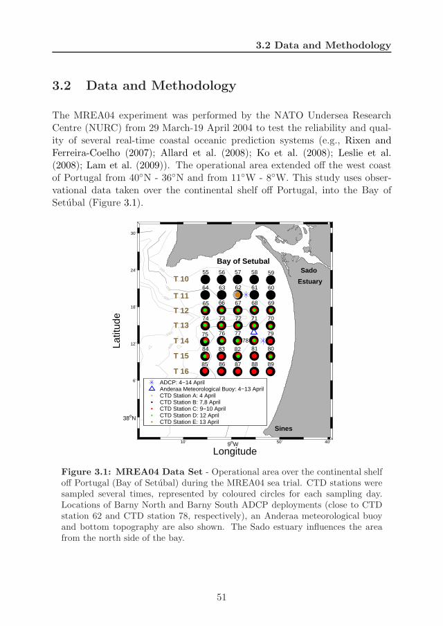
3.2 Data and Methodology
3.2 Data and Methodology
The MREA04 experiment was performed by the NATO Undersea ResearchCentre (NURC) from 29 March-19 April 2004 to test the reliability and qual-ity of several real-time coastal oceanic prediction systems (e.g., Rixen andFerreira-Coelho (2007); Allard et al. (2008); Ko et al. (2008); Leslie et al.(2008); Lam et al. (2009)). The operational area extended off the west coastof Portugal from 40N - 36N and from 11W - 8W. This study uses obser-vational data taken over the continental shelf off Portugal, into the Bay ofSetubal (Figure 3.1).
Longitude
Latit
ude
−100
−500
−1000
−800
−20055 56 57 58 59
6061626364
65 66 67 68 69
7071727374
75 76 77 79
8081828384
85 86 87 88 89
78
T 10
T 11
T 12
T 13
T 14
T 15
T 16
10’ 9oW 50’ 40’
38oN
6’
12’
18’
24’
30’
Bay of Setubal
Sines
Sado
Estuary
ADCP: 4−14 AprilAnderaa Meteorological Buoy: 4−13 AprilCTD Station A: 4 AprilCTD Station B: 7,8 AprilCTD Station C: 9−10 AprilCTD Station D: 12 AprilCTD Station E: 13 April
Figure 3.1: MREA04 Data Set - Operational area over the continental shelfoff Portugal (Bay of Setubal) during the MREA04 sea trial. CTD stations weresampled several times, represented by coloured circles for each sampling day.Locations of Barny North and Barny South ADCP deployments (close to CTDstation 62 and CTD station 78, respectively), an Anderaa meteorological buoyand bottom topography are also shown. The Sado estuary influences the areafrom the north side of the bay.
51
3. BREEZE-FORCED OSC. AND DIAPYCNAL MIXING
This region is characterised by a steep bathymetry because of the SetubalCanyon, and by fluvial inputs coming from the Sado estuary on the northernside of the bay. Related to tides, the Bay of Setubal is mainly dominated bylunar (M2) and solar (S2) semidiurnal components (Martins et al., 2002).
Vertical temperature and salinity profiles were obtained using Seabird 911Plus CTD real-time pumped systems. The CTD stations were sampled severaltimes to get incoming temperature and salinity data in real-time to run, correctand compare the forecasts made by the coastal oceanic prediction modelstested during the MREA04 trial. A total of 195 CTD casts were distributedamong 95 different sites over the continental shelf and open ocean area from31 March-16 April 2004. In this chapter, we present the 35 different sitesthat were analised to get an overview of the coastal ocean conditions involvingthe observed breeze-forced oscillations, and study the associated diapycnalmixing processes into the Bay of Setubal. These sites spanned a regular CTDgrid with a spatial resolution of 5 km between CTD stations and transects(Figure 3.1).
Currents data were obtained from two RDI Workhorse ADCP’s deployedon Barny-type trawl safe platforms and situated on the north (Barny NorthADCP) and south (Barny South ADCP) sides of the bay at 106,6 m and 118 mdepth, respectively (Figure 3.1). Both deployments of Barny Sentinel ADCP’srecorded vertical profiles of horizontal velocity (u, v) with a broadband of307.2 kHz and 24 bins of 4 m size. The ADCP heads were about 6 m fromthe bottom. Both profilers sampled data once every minute for the period of4 − 14 April 2004.
The rotary spectral method (Hayashi, 1979; van Aken et al., 2005) wasapplied to examine the variance in the current oscillations for each frequencyband as clockwise and counterclockwise rotating variances. Because breeze-forced oscillations involve currents rotating in a clockwise (counterclockwise)direction in the Northern (Southern) Hemisphere, this technique contributesto determining its presence.
Next the diurnal-inertial band, in which breeze-forced oscillation peak,was isolated from the rest of the frequencies to characterise its properties.Previously, to filter this band, the original current records were decimatedto 1 datum per hour after lowpass filtering. Then frequency-band of inter-est was isolated via band-pass filtering with a fourth-order Butterworth filterwith zero-phase response and quarter-power points at c−1ωc, c ωc around
52
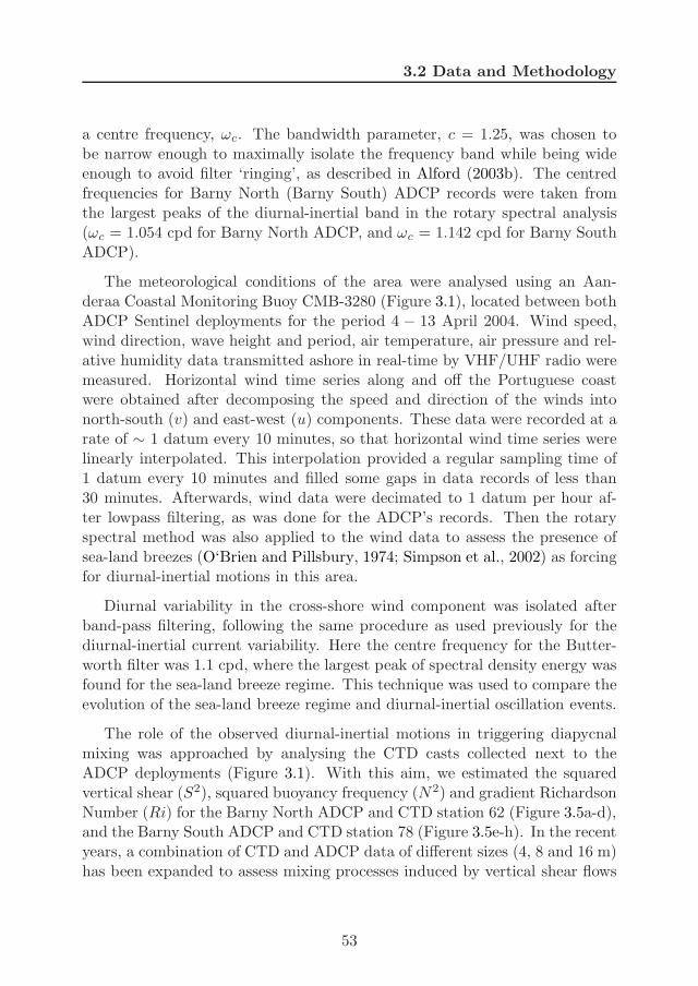
3.2 Data and Methodology
a centre frequency, ωc. The bandwidth parameter, c = 1.25, was chosen tobe narrow enough to maximally isolate the frequency band while being wideenough to avoid filter ‘ringing’, as described in Alford (2003b). The centredfrequencies for Barny North (Barny South) ADCP records were taken fromthe largest peaks of the diurnal-inertial band in the rotary spectral analysis(ωc = 1.054 cpd for Barny North ADCP, and ωc = 1.142 cpd for Barny SouthADCP).
The meteorological conditions of the area were analysed using an Aan-deraa Coastal Monitoring Buoy CMB-3280 (Figure 3.1), located between bothADCP Sentinel deployments for the period 4 − 13 April 2004. Wind speed,wind direction, wave height and period, air temperature, air pressure and rel-ative humidity data transmitted ashore in real-time by VHF/UHF radio weremeasured. Horizontal wind time series along and off the Portuguese coastwere obtained after decomposing the speed and direction of the winds intonorth-south (v) and east-west (u) components. These data were recorded at arate of ∼ 1 datum every 10 minutes, so that horizontal wind time series werelinearly interpolated. This interpolation provided a regular sampling time of1 datum every 10 minutes and filled some gaps in data records of less than30 minutes. Afterwards, wind data were decimated to 1 datum per hour af-ter lowpass filtering, as was done for the ADCP’s records. Then the rotaryspectral method was also applied to the wind data to assess the presence ofsea-land breezes (O‘Brien and Pillsbury, 1974; Simpson et al., 2002) as forcingfor diurnal-inertial motions in this area.
Diurnal variability in the cross-shore wind component was isolated afterband-pass filtering, following the same procedure as used previously for thediurnal-inertial current variability. Here the centre frequency for the Butter-worth filter was 1.1 cpd, where the largest peak of spectral density energy wasfound for the sea-land breeze regime. This technique was used to compare theevolution of the sea-land breeze regime and diurnal-inertial oscillation events.
The role of the observed diurnal-inertial motions in triggering diapycnalmixing was approached by analysing the CTD casts collected next to theADCP deployments (Figure 3.1). With this aim, we estimated the squaredvertical shear (S2), squared buoyancy frequency (N2) and gradient RichardsonNumber (Ri) for the Barny North ADCP and CTD station 62 (Figure 3.5a-d),and the Barny South ADCP and CTD station 78 (Figure 3.5e-h). In the recentyears, a combination of CTD and ADCP data of different sizes (4, 8 and 16 m)has been expanded to assess mixing processes induced by vertical shear flows
53
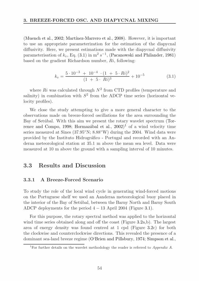
3. BREEZE-FORCED OSC. AND DIAPYCNAL MIXING
(Muench et al., 2002; Martınez-Marrero et al., 2008). However, it is importantto use an appropriate parameterization for the estimation of the diapycnaldiffusivity. Here, we present estimations made with the diapycnal diffusivityparameterisation of kv, Eq. (3.1) in m2 s−1, (Pacanowski and Philander, 1981)based on the gradient Richardson number, Ri, following:
kv =5 · 10−3 + 10−4 · (1 + 5 · Ri)2
(1 + 5 · Ri)3+ 10−5 (3.1)
where Ri was calculated through N2 from CTD profiles (temperature andsalinity) in combination with S2 from the ADCP time series (horizontal ve-locity profiles).
We close the study attempting to give a more general character to theobservations made on breeze-forced oscillations for the area surrounding theBay of Setubal. With this aim we present the rotary wavelet spectrum (Tor-rence and Compo, 1998; Hormazabal et al., 2002)1 of a wind velocity timeseries measured at Sines (37.95N; 8.88W) during the 2004. Wind data wereprovided by the Instituto Hidrografico - Portugal and recorded with an An-deraa meteorological station at 35.1 m above the mean sea level. Data weremeasured at 10 m above the ground with a sampling interval of 10 minutes.
3.3 Results and Discussion
3.3.1 A Breeze-Forced Scenario
To study the role of the local wind cycle in generating wind-forced motionson the Portuguese shelf we used an Aanderaa meteorological buoy placed inthe interior of the Bay of Setubal, between the Barny North and Barny SouthADCP deployments for the period 4 − 13 April 2004 (Figure 3.1).
For this purpose, the rotary spectral method was applied to the horizontalwind time series obtained along and off the coast (Figure 3.2a,b). The largestarea of energy density was found centred at 1 cpd (Figure 3.2c) for boththe clockwise and counterclockwise directions. This revealed the presence of adominant sea-land breeze regime (O‘Brien and Pillsbury, 1974; Simpson et al.,
1For further details on the wavelet methodology the reader is referred to Appendix A.
54
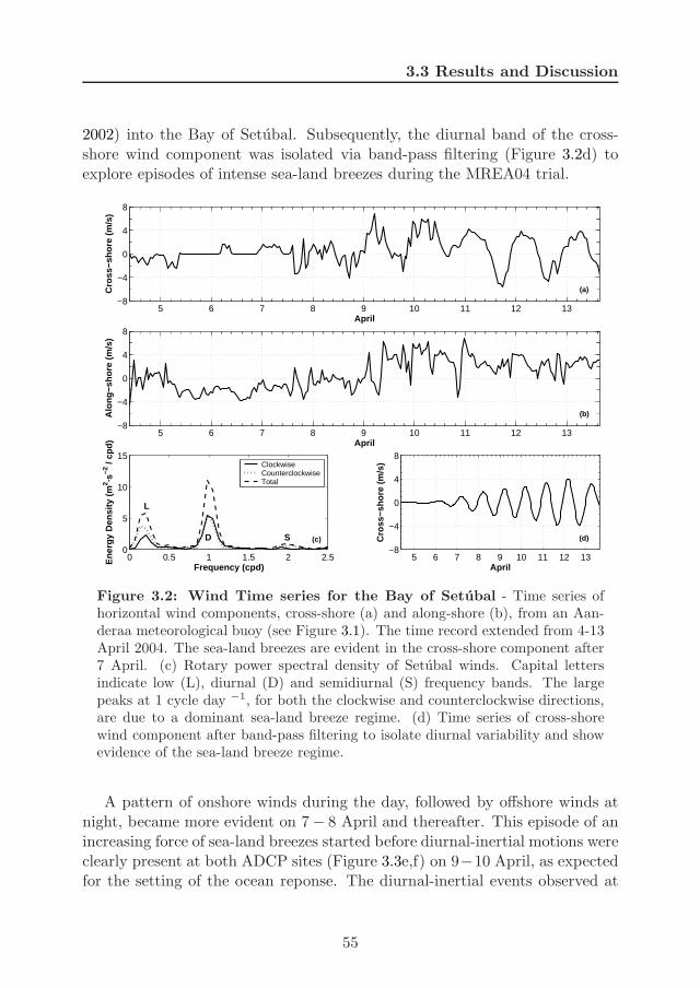
3.3 Results and Discussion
2002) into the Bay of Setubal. Subsequently, the diurnal band of the cross-shore wind component was isolated via band-pass filtering (Figure 3.2d) toexplore episodes of intense sea-land breezes during the MREA04 trial.
5 6 7 8 9 10 11 12 13−8
−4
0
4
8
April
Alo
ng−s
hore
(m
/s)
(b)
5 6 7 8 9 10 11 12 13−8
−4
0
4
8
April
Cro
ss−s
hore
(m
/s)
(a)
5 6 7 8 9 10 11 12 13−8
−4
0
4
8
April
Cro
ss−s
hore
(m
/s)
(d)
0 0.5 1 1.5 2 2.50
5
10
15
Frequency (cpd)
Ene
rgy
Den
sity
(m
2 ·s−2
/ cp
d)
(c)
L
D S
ClockwiseCounterclockwiseTotal
Figure 3.2: Wind Time series for the Bay of Setubal - Time series ofhorizontal wind components, cross-shore (a) and along-shore (b), from an Aan-deraa meteorological buoy (see Figure 3.1). The time record extended from 4-13April 2004. The sea-land breezes are evident in the cross-shore component after7 April. (c) Rotary power spectral density of Setubal winds. Capital lettersindicate low (L), diurnal (D) and semidiurnal (S) frequency bands. The largepeaks at 1 cycle day −1, for both the clockwise and counterclockwise directions,are due to a dominant sea-land breeze regime. (d) Time series of cross-shorewind component after band-pass filtering to isolate diurnal variability and showevidence of the sea-land breeze regime.
A pattern of onshore winds during the day, followed by offshore winds atnight, became more evident on 7 − 8 April and thereafter. This episode of anincreasing force of sea-land breezes started before diurnal-inertial motions wereclearly present at both ADCP sites (Figure 3.3e,f) on 9−10 April, as expectedfor the setting of the ocean reponse. The diurnal-inertial events observed at
55
3. BREEZE-FORCED OSC. AND DIAPYCNAL MIXING
the beginning of the Barny North record, on 4 − 6 April (Figure 3.3e), mightalso be the consequence of a sea-land breeze regime forcing the bay a few daysbefore initiation of the meteorological buoy record. During the MREA04 seatrial, we found values for this wind cycle with a maximum speed of about4 m s−1, within the typical range of 2 − 5 m s−1 reported for sea-land breezeregimes (Simpson et al., 2002).
3.3.2 Breeze-Forced Oscillations
During the MREA04 sea trial, diurnal-inertial events were recorded in theBay of Setubal (Figure 3.1) at the Barny North and Barny South ADCP sites(∼ 38 N), where diurnal and inertial frequencies approach each other andbreeze-forced oscillations may be enhanced. Decimated time series from thesecurrent profilers are shown in Figure 3.3a,b.
The depth-averaged rotary power spectral density for both ADCP locations(Figure 3.3c,d) shows that currents within the diurnal-inertial band were dom-inated by circular, clockwise motions. Here we define the diurnal-inertial bandas approximately between 0.88 cpd and 1.38 cpd and involving both the di-urnal (ωd = 1 cpd) and inertial frequencies (f ∼ 1.24 cpd about 38 N). Thecentral peak of this band (ωc ∼1.1 cpd) was found at both sites in between ωd
and f . The proximity between these two frequencies, together with the lengthof the ADCP records, prevent us from distinguishing dominant peaks aroundωd and f .
For the most part, the diurnal-inertial band showed higher energy densitiesthan did the semidiurnal band at both locations. Nevertheless, a strong varia-tion in energy distribution was observed between the Barny North and BarnySouth records for this frequency-band that was more energetic at the BarnyNorth ADCP site. Semidiurnal currents also exhibited different features, de-pending on the location. Elliptical clockwise gyres, 1 order of magnitudesmaller than the diurnal-inertial band, were found to dominate at the BarnyNorth ADCP site (Figure 3.3c), whereas elliptical counterclockwise gyres withthe same order of magnitude as the diurnal-inertial band were found at theBarny South ADCP site (Figure 3.3d).
56
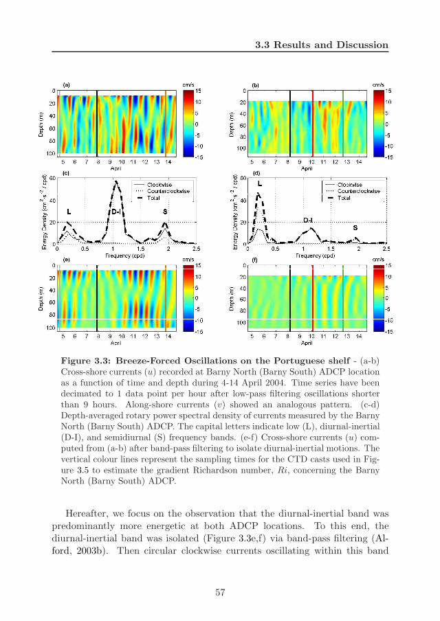
3.3 Results and Discussion
Figure 3.3: Breeze-Forced Oscillations on the Portuguese shelf - (a-b)Cross-shore currents (u) recorded at Barny North (Barny South) ADCP locationas a function of time and depth during 4-14 April 2004. Time series have beendecimated to 1 data point per hour after low-pass filtering oscillations shorterthan 9 hours. Along-shore currents (v) showed an analogous pattern. (c-d)Depth-averaged rotary power spectral density of currents measured by the BarnyNorth (Barny South) ADCP. The capital letters indicate low (L), diurnal-inertial(D-I), and semidiurnal (S) frequency bands. (e-f) Cross-shore currents (u) com-puted from (a-b) after band-pass filtering to isolate diurnal-inertial motions. Thevertical colour lines represent the sampling times for the CTD casts used in Fig-ure 3.5 to estimate the gradient Richardson number, Ri, concerning the BarnyNorth (Barny South) ADCP.
Hereafter, we focus on the observation that the diurnal-inertial band waspredominantly more energetic at both ADCP locations. To this end, thediurnal-inertial band was isolated (Figure 3.3e,f) via band-pass filtering (Al-ford, 2003b). Then circular clockwise currents oscillating within this band
57
3. BREEZE-FORCED OSC. AND DIAPYCNAL MIXING
(Figure 3.3c,d) were characterised in a two-layer configuration with a phaseshift of ∼180 between the upper and lower layers at both ADCP locations.Thereof, maximum current amplitudes of approximately 15 cm s−1 were foundat the upper and lower layers for the Barny North ADCP location (Figure 3.3e)when diurnal wind forcing increased during 10−13 April (Figure 3.2d), whereasthe maximum values were weaker, at approximately 5 cm s−1, for the sameperiod at the Barny South ADCP location. This period of increasing diurnalwind forcing appeared after 3 days of wind relaxation on 4−7 April. However,we also found evidence of diurnal-inertial oscillations with amplitudes of ap-proximately 10 cm s−1 on those days at the Barny North site (Figure 3.3e). Aswe previously pointed out, these oscillations might be the transient responseto a sea-land breeze regime that was acting a few days before the initiation ofthe meteorological buoy record and vanished later, what lead to wind-forceddiurnal-inertial oscillations evolving into free near-inertial oscillations (Rip-peth et al., 2002; Simpson et al., 2002). This situation would support thecentral peak (ωc) of the diurnal-inertial band being band between ωd and f asa combination of breeze-forced diurnal oscillations and transient near-inertialoscillations that come into play when wind forcing diminishes (Figure 3.3c,d).
According to the barotropic pressure gradient set up by breeze forcing atsurface and its response in antiphase at the lower layer (Hyder et al., 2002;Rippeth et al., 2002; Simpson et al., 2002), the resultant breeze-forced oscil-lations showed, within every layer, very small variations in phase with depth.Additionally, the interface related to this 180 phase shift seemed to be fixedat a certain depth at both ADCP locations (∼ 40 m at Barny North and ∼30 m at Barny South), except for the period 10 − 14 April when the depth ofthe phase shift moved downward along the Barny North ADCP record from40 m to 70 m (Figure 3.3e). This deepening of the interface might have beena consequence to increasing diurnal wind intensities during those days (Fig-ure 3.2d), in combination with a deepening of the pycnocline also from 40 mto 70 m (7-13 April in Figure 3.5a) owing to diapycnal mixing processes (asit will be analysed in Section 3.3.4). This observation agrees with previousworks of modeling (Rippeth et al., 2002) in which the vertical structure ofbreeze-forced oscillatitons is driven by the above mentioned pressure gradientforcing, but the pycnocline marks the depth at which the phase shift is set up.Because of this behaviour, it was not rare to find a weakening of the diurnal-inertial vertical structure at the Barny North ADCP after 13 April, when thesupport of the interface had been strongly eroded and motions related to in-ertial contribution were damped out in the absence of a sharped pycnocline
58
3.3 Results and Discussion
(as also shown in Rippeth et al. (2002)).
In modeling these energetic oscillations for MREA exercises, it is importantto highlight that these are essentially wind-forced motions. Therefore, accuratemeteorological forcing represents a critical target to get realistic predictionsin real-time, similar to previous suggestions for near-inertial motions observedduring the Maritime Rapid Environmental Assessment 2003 (MREA03) exer-cise, which was performed off of the west coast of Italy near the Elba Island(Coelho and Robinson, 2003). It has been attempted (research not shownhere) to forecast the observed breeze-forced oscillations with a coastal oceanicprediction model around the ADCP’s sites during the MREA04 sea trial. Testswere capable of reproducing the essential physics of these oscillations, althoughthe forecasted oscillations are weaker and phase lagged in comparison with theobservations. Recent efforts and improvements have been done in modelingfor MREA exercises with adaptive sampling on short-time scales (Wang et al.,2009; Haley and Lermusiaux, 2010; Lermusiaux et al., 2010; Ueckermann andLermusiaux, 2010).
3.3.3 Diapycnal Mixing and Breeze-Forced Events
The role that observed breeze-forced oscillations could be playing in the inte-rior of the Bay of Setubal responds to its associated high vertical shear withinstratified layers (Pelegrı and Sangra, 1998; Rodrıguez-Santana et al., 1999,2001) and is discussed here in terms of diapycnal mixing processes.
The entire Bay of Setubal exhibited different stages of stratification duringthe MRE04 sea trial that involved breeze-forced oscillations and intrusions offluvial waters coming from the Sado estuary. As is shown by the surface salin-ity and potential density fields in Figure 3.4a,d, this estuarine signal stronglyaffected the northern and western sides of the bay on 7-8 April, enlarging thearea influenced on 9-10 April (Figure 3.4b,e). After a few days, this lighterand freshwater signal had already disappeared (12 April; Figure 3.4c,f). In thefollowing we assess breeze-forced currents triggering diapycnal vertical mixingbetween oceanic and estuarine waters in the interior of the bay. We focus onthat scenario accounting for the interaction between diurnal-inertial oscillationcurrent events and stratification due to freshwater inputs.
59
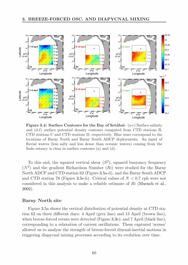
3. BREEZE-FORCED OSC. AND DIAPYCNAL MIXING
Longitude
Latit
ude
12’ 6’ 9oW 54’ 48’ 42’ 5’
10’
38oN 15.00’
20’
25’
30’
7−8 AprilT 10
T 11
T 12
T 13
T 14
T 15
T 16(a)
Longitude
Latit
ude
12’ 6’ 9oW 54’ 48’ 42’ 5’
10’
38oN 15.00’
20’
25’
30’
7−8 AprilT 10
T 11
T 12
T 13
T 14
T 15
T 16(d)
Longitude 12’ 6’ 9oW 54’ 48’ 42’
5’
10’
38oN 15.00’
20’
25’
30’
9−10 April
T 13
T 14
T 15
T 16(b)
Longitude 12’ 6’ 9oW 54’ 48’ 42’
5’
10’
38oN 15.00’
20’
25’
30’
9−10 April
T 13
T 14
T 15
T 16(e)
Longitude 12’ 6’ 9oW 54’ 48’ 42’
5’
10’
38oN 15.00’
20’
25’
30’
12 April
T 12
T 13
T 14
T 15
(c)35.7
35.75
35.8
35.85
35.9
35.95
36
36.05
Longitude 12’ 6’ 9oW 54’ 48’ 42’
5’
10’
38oN 15.00’
20’
25’
30’
12 April
T 12
T 13
T 14
T 15
(f)
kg·m−3
26.4
26.5
26.6
26.7
26.8
Figure 3.4: Surface Contours for the Bay of Setubal - (a-c) Surface salinityand (d-f) surface potential density contours computed from CTD stations B,CTD stations C and CTD stations D, respectively. Blue stars correspond to thelocations of Barny North and Barny South ADCP deployments. An input offluvial waters (less salty and less dense than oceanic waters) coming from theSado estuary is clear in surface contours (a) and (d).
To this end, the squared vertical shear (S2), squared buoyancy frequency(N2) and the gradient Richardson Number (Ri) were studied for the BarnyNorth ADCP and CTD station 62 (Figure 3.5a-d), and the Barny South ADCPand CTD station 78 (Figure 3.5e-h). Critical values of N < 0.7 cph were notconsidered in this analysis to make a reliable estimate of Ri (Muench et al.,2002).
Barny North site
Figure 3.5a shows the vertical distribution of potential density at CTD sta-tion 62 on three different days: 4 April (grey line) and 13 April (brown line),when breeze-forced events were detected (Figure 3.3e); and 7 April (black line),corresponding to a relaxation of current oscillations. These captured ‘scenes’allowed us to analyse the strength of breeze-forced diurnal-inertial motions intriggering diapycnal mixing processes according to its evolution over time.
60
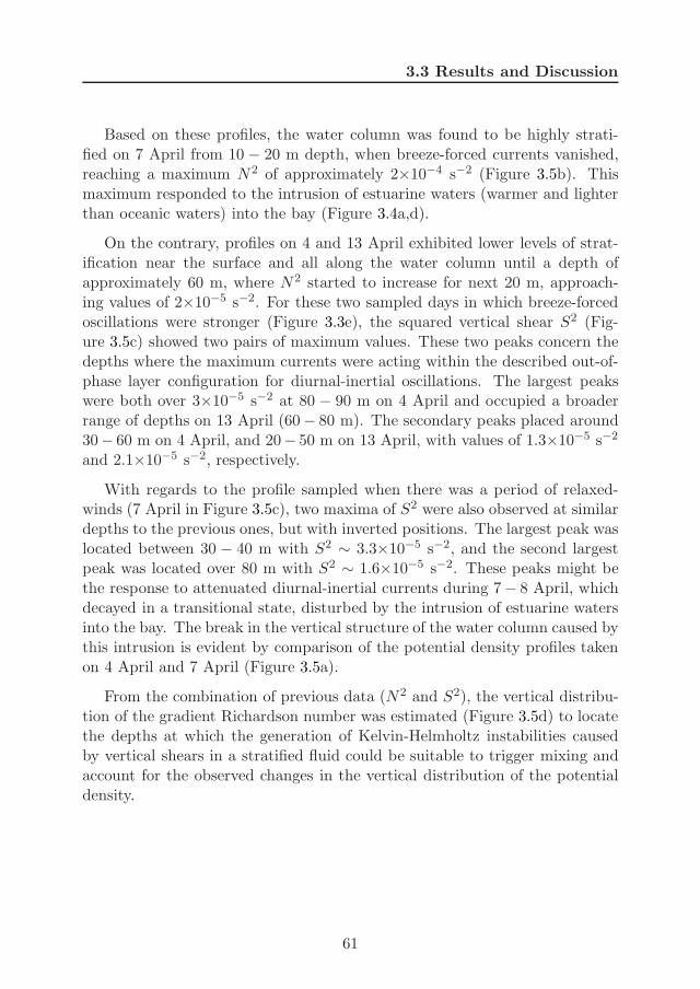
3.3 Results and Discussion
Based on these profiles, the water column was found to be highly strati-fied on 7 April from 10 − 20 m depth, when breeze-forced currents vanished,reaching a maximum N2 of approximately 2×10⁻⁴ s−2 (Figure 3.5b). Thismaximum responded to the intrusion of estuarine waters (warmer and lighterthan oceanic waters) into the bay (Figure 3.4a,d).
On the contrary, profiles on 4 and 13 April exhibited lower levels of strat-ification near the surface and all along the water column until a depth ofapproximately 60 m, where N2 started to increase for next 20 m, approach-ing values of 2×10⁻⁵ s−2. For these two sampled days in which breeze-forcedoscillations were stronger (Figure 3.3e), the squared vertical shear S2 (Fig-ure 3.5c) showed two pairs of maximum values. These two peaks concern thedepths where the maximum currents were acting within the described out-of-phase layer configuration for diurnal-inertial oscillations. The largest peakswere both over 3×10⁻⁵ s−2 at 80 − 90 m on 4 April and occupied a broaderrange of depths on 13 April (60− 80 m). The secondary peaks placed around30− 60 m on 4 April, and 20− 50 m on 13 April, with values of 1.3×10⁻⁵ s−2
and 2.1×10⁻⁵ s−2, respectively.
With regards to the profile sampled when there was a period of relaxed-winds (7 April in Figure 3.5c), two maxima of S2 were also observed at similardepths to the previous ones, but with inverted positions. The largest peak waslocated between 30 − 40 m with S2 ∼ 3.3×10⁻⁵ s−2, and the second largestpeak was located over 80 m with S2 ∼ 1.6×10⁻⁵ s−2. These peaks might bethe response to attenuated diurnal-inertial currents during 7− 8 April, whichdecayed in a transitional state, disturbed by the intrusion of estuarine watersinto the bay. The break in the vertical structure of the water column caused bythis intrusion is evident by comparison of the potential density profiles takenon 4 April and 7 April (Figure 3.5a).
From the combination of previous data (N2 and S2), the vertical distribu-tion of the gradient Richardson number was estimated (Figure 3.5d) to locatethe depths at which the generation of Kelvin-Helmholtz instabilities causedby vertical shears in a stratified fluid could be suitable to trigger mixing andaccount for the observed changes in the vertical distribution of the potentialdensity.
61
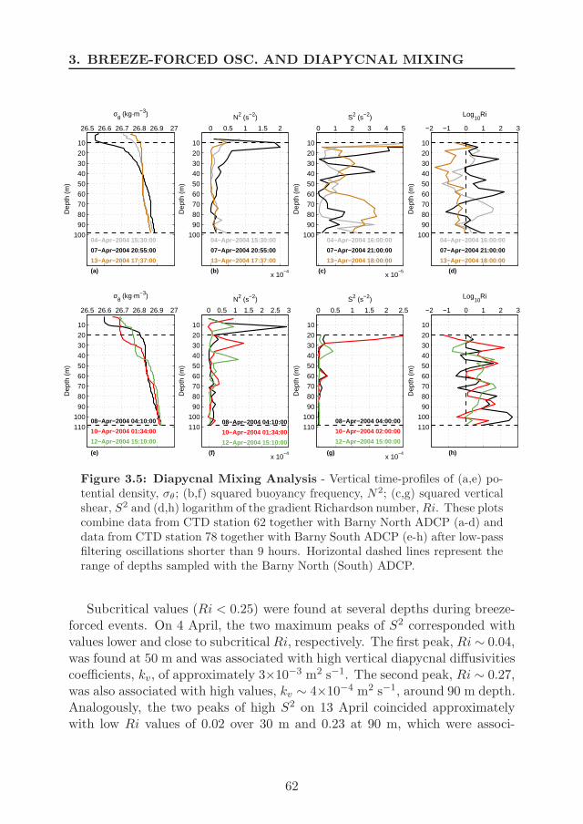
3. BREEZE-FORCED OSC. AND DIAPYCNAL MIXING
26.5 26.6 26.7 26.8 26.9 27
10
20
30
40
50
60
70
80
90
100
σθ (kg·m−3)
Dep
th (
m)
04−Apr−2004 15:30:00
07−Apr−2004 20:55:00
13−Apr−2004 17:37:00
(a)
0 0.5 1 1.5 2
x 10−4
10
20
30
40
50
60
70
80
90
100
N2 (s−2)
Dep
th (
m)
04−Apr−2004 15:30:00
07−Apr−2004 20:55:00
13−Apr−2004 17:37:00
(b)
0 1 2 3 4 5
x 10−5
10
20
30
40
50
60
70
80
90
100
S2 (s−2)
Dep
th (
m)
04−Apr−2004 16:00:00
07−Apr−2004 21:00:00
13−Apr−2004 18:00:00
(c)
−2 −1 0 1 2 3
10
20
30
40
50
60
70
80
90
100
Log10
Ri
Dep
th (
m)
04−Apr−2004 16:00:00
07−Apr−2004 21:00:00
13−Apr−2004 18:00:00
(d)
26.5 26.6 26.7 26.8 26.9 27
10
20
30
40
50
60
70
80
90
100
110
σθ (kg·m−3)
Dep
th (
m)
08−Apr−2004 04:10:00
10−Apr−2004 01:34:00
12−Apr−2004 15:10:00
(e)
0 0.5 1 1.5 2 2.5 3
x 10−4
10
20
30
40
50
60
70
80
90
100
110
N2 (s−2)
Dep
th (
m)
08−Apr−2004 04:10:00
10−Apr−2004 01:34:00
12−Apr−2004 15:10:00
(f)
0 0.5 1 1.5 2 2.5
x 10−4
10
20
30
40
50
60
70
80
90
100
110
S2 (s−2)D
epth
(m
)
08−Apr−2004 04:00:00
10−Apr−2004 02:00:00
12−Apr−2004 15:00:00
(g)
−2 −1 0 1 2 3
10
20
30
40
50
60
70
80
90
100
110
Log10
Ri
Dep
th (
m)
(h)
Figure 3.5: Diapycnal Mixing Analysis - Vertical time-profiles of (a,e) po-tential density, σθ; (b,f) squared buoyancy frequency, N2; (c,g) squared verticalshear, S2 and (d,h) logarithm of the gradient Richardson number, Ri. These plotscombine data from CTD station 62 together with Barny North ADCP (a-d) anddata from CTD station 78 together with Barny South ADCP (e-h) after low-passfiltering oscillations shorter than 9 hours. Horizontal dashed lines represent therange of depths sampled with the Barny North (South) ADCP.
Subcritical values (Ri < 0.25) were found at several depths during breeze-forced events. On 4 April, the two maximum peaks of S2 corresponded withvalues lower and close to subcritical Ri, respectively. The first peak, Ri ∼ 0.04,was found at 50 m and was associated with high vertical diapycnal diffusivitiescoefficients, kv, of approximately 3×10⁻³ m2 s−1. The second peak, Ri ∼ 0.27,was also associated with high values, kv ∼ 4×10⁻⁴ m2 s−1, around 90 m depth.Analogously, the two peaks of high S2 on 13 April coincided approximatelywith low Ri values of 0.02 over 30 m and 0.23 at 90 m, which were associ-
62

3.3 Results and Discussion
ated with an enhanced kv of ∼ 4×10⁻³ and ∼ 5×10⁻⁴ m2 s−1, respectively.Overall, on 13 April, the whole profile supported values of Ri < 1, givingrise to high diapycnal diffusivities, especially in the range of the upper layer(20-50 m depth) observed for breeze-forced oscillations during 10 − 14 April(Figure 3.3e).
It is worth noting that, during the breeze-relaxed period on 7− 8 April, Rivalues larger than 1 were obtained with high levels of high stratification nearthe surface and attributable to strong inputs of fluvial waters on these days.Nevertheless, at deeper levels (around 80 m), Ri values close to 0.1 were alsofound with kv ∼ 2×10⁻³ m2 s−1.
The common pattern observed on 4 and 13 April during breeze-forced cur-rent events was a two-layer vertical structure with high values of S2 embeddingstratified waters. As a result, the pycnocline that partially contributed to sup-porting this two-layer configuration was significantly eroded. In such a way,this triggered a vertical displacement of the interface with high stratification,now smoothed, towards deeper waters. These results suggest that the dis-placement was promoted by the high vertical shear of the upper and lowerlayers acting over the depths of the highest stratification.
If we now recall the theoretical works of Rippeth et al. (2002) and Simpsonet al. (2002), one can understand why in presence of a noticeable breeze-forcing over 8-13 April (Figure 3.2d) there is, on the contrary, a weakeningof the breeze-forced current system. These studies predict that breeze-forcedcurrents at the lower layer, in relation to those in the upper layer, vanish by afactor γ which is dependent of the depth of the pycnocline following γ = h2/h1
(being h1 (h2) the thickness of the upper (lower layer)). Thus, the deepeningand smoothing of the interface observed along 8-13 April (Figure 3.5a-d) couldhave driven the self erosion of the baroclinic mode which supported the breeze-forced current system (Figure 3.3e) owing to its associated vertical diapycnalmixing. A similar finding was reported by Zhang et al. (2009) in the Gulfof Mexico, where they observed that the deepening of the mixed layer depthdriven by freshwater inputs and vertical mixing weakened the diurnal-inertialocean response to breeze-forcing.
Barny South site
Regarding the Barny South ADCP deployment and CTD station 78, Fig-ure 3.5e presents the vertical profiles of potential density on three different
63

3. BREEZE-FORCED OSC. AND DIAPYCNAL MIXING
days: 8 April (black line), characterised by the absence of breeze-forced events;and 10 April (red line) and 12 April (green line), which involved increasingbreeze-forced oscillations (Figure 3.3e).
As can be observed in Figure 3.5f, the maximum values of N2 that partiallysupported the baroclinic mode of these diurnal-inertial motions increased theirdepth from 8 April (10 m) to 12 April (45 m) while decreasing their values fromapproximately 3×10⁻⁴ s−2 to 1×10⁻⁴ s−2. This deepening of the pycnoclinelikely occurred according to the mechanism previously explained for breeze-forced currents oscillating around the Barny North ADCP site.
On 10 April, the distribution of vertical shear (Figure 3.5g) exhibited amaximum at 20 m, which was above the interface of high stratification, withan S2 of approximately 2.7×10⁻⁴ s−2. A secondary peak of S2 ∼ 3×10⁻⁵ s−2
was found on the same day for the lower layers, which is similar to the situationdescribed for the Barny North ADCP. Likewise, on 12 April, a maximum ofS2 was also found above the interface of high stratification with values of∼ 4.3×10⁻⁵ s−2 at approximately 35 m.
For days when breeze-forced diurnal-inertial oscillations were acting, themain peaks of S2 coincided with low Ri values of 0.05 at 20 m depth on10 April and 0.17 at 35 m depth on 12 April (Figure 3.5h). The values ofkv associated with these Ri values were also relatively high, approximately2.6×10−3 m2 s−1 on 10 April and 8×10⁻⁴ m2 s−1 on 12 April. As a conse-quence, the combination of strong vertical shears and surface inputs of strati-fication from the estuary produced the same effects as illustrated for the areasampled by the Barny North ADCP and CTD station 62. Thus, a notice-able modification of the density vertical distribution at relatively short-timescales was also found in response to diapycnal mixing processes enhanced bybreeze-forced motions. Additionally, it was also found that again the well-defined baroclinic mode structure which supported the breeze-forced currents(Figure 3.5e-h on 10 April) broke up due to vertical mixing (Figure 3.5e-h on12 April), hence weakening the diurnal-inertial ocean response even in presenceof breeze-forcing (Figure 3.3f).
CTD and ADCP observations reported here, although they were not plannedduring the MREA04 sea trial for the present research, successfully capture thecritical moments and consequences of the interactions between breeze-forcedcurrent events and stratified waters in the interior of the bay. These resultscontribute to explaining the main vertical changes observed in the CTD casts
64
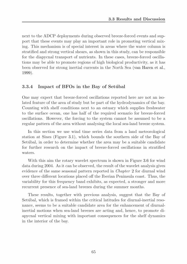
3.3 Results and Discussion
next to the ADCP deployments during observed breeze-forced events and sup-port that these events may play an important role in promoting vertical mix-ing. This mechanism is of special interest in areas where the water column isstratified and strong vertical shears, as shown in this study, can be responsiblefor the diapycnal transport of nutrients. In these cases, breeze-forced oscilla-tions may be able to promote regions of high biological productivity, as it hasbeen observed for strong inertial currents in the North Sea (van Haren et al.,1999).
3.3.4 Impact of BFOs in the Bay of Setubal
One may expect that breeze-forced oscillations reported here are not an iso-lated feature of the area of study but be part of the hydrodynamics of the bay.Counting with shelf conditions next to an estuary which supplies freshwaterto the surface ocean, one has half of the required scenario for breeze-forcedoscillations. However, the forcing to the system cannot be assumed to be aregular pattern of the area without analysing the local sea-land breeze system.
In this section we use wind time series data from a land meteorologicalstation at Sines (Figure 3.1), which bounds the southern side of the Bay ofSetubal, in order to determine whether the area may be a suitable candidatefor further research on the impact of breeze-forced oscillations in stratifiedwaters.
With this aim the rotary wavelet spectrum is shown in Figure 3.6 for winddata during 2004. As it can be observed, the result of the wavelet analysis givesevidence of the same seasonal pattern reported in Chapter 2 for diurnal windover three different locations placed off the Iberian Peninsula coast. Thus, thevariability for this frequency band exhibits, as expected, a stronger and morerecurrent presence of sea-land breezes during the summer months.
These results, together with previous analysis, suggest that the Bay ofSetubal, which is framed within the critical latitudes for diurnal-inertial reso-nance, seems to be a suitable candidate area for the enhancement of diurnal-inertial motions when sea-land breezes are acting and, hence, to promote di-apycnal vertical mixing with important consequences for the shelf dynamicsin the interior of the bay.
65
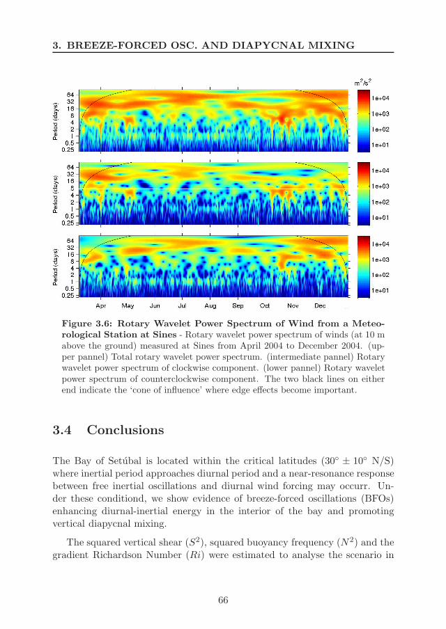
3. BREEZE-FORCED OSC. AND DIAPYCNAL MIXING
Figure 3.6: Rotary Wavelet Power Spectrum of Wind from a Meteo-rological Station at Sines - Rotary wavelet power spectrum of winds (at 10 mabove the ground) measured at Sines from April 2004 to December 2004. (up-per pannel) Total rotary wavelet power spectrum. (intermediate pannel) Rotarywavelet power spectrum of clockwise component. (lower pannel) Rotary waveletpower spectrum of counterclockwise component. The two black lines on eitherend indicate the ‘cone of influence’ where edge effects become important.
3.4 Conclusions
The Bay of Setubal is located within the critical latitudes (30 ± 10 N/S)where inertial period approaches diurnal period and a near-resonance responsebetween free inertial oscillations and diurnal wind forcing may occurr. Un-der these conditiond, we show evidence of breeze-forced oscillations (BFOs)enhancing diurnal-inertial energy in the interior of the bay and promotingvertical diapycnal mixing.
The squared vertical shear (S2), squared buoyancy frequency (N2) and thegradient Richardson Number (Ri) were estimated to analyse the scenario in
66

3.4 Conclusions
which enhanced vertical shears developed during breeze-forced events led tostratified and vertically sheared flows with subcritical values of Ri. Thesezones were found to promote vertical mixing across the pycnocline due tostrong squared vertical shears about 10−5 s−2. In the end, these mixing pro-cesses drove the self-erosion of the pycnocline that partially supported theinterface between the two-layers, thereby homogenising the water column intheir wake. At the Barny South ADCP site, the vertical variation in the high-est peaks of stratification was especially clear, shifting approximately 15 m intwo and a half days and involving an efficient mechanism to transport prop-erties vertically throughout the water column.
The above results point out that there may exist an internal control on thestrength of the ocean response to breeze forcing that has not been describedbefore to the best of our knowledge. This follows from the previously dis-cussed role that the depth of the mixed layer plays on the vertical structureof BFOs supporting its baroclinic mode and determining the intensity of theforced currents above and below the pycnocline (Rippeth et al., 2002; Simpsonet al., 2002). Starting from this basis, we observe that vertical diapycnal mix-ing promoted by breeze-forced oscillations led to the deepening and smoothingof the pycnocline which supported them and, hence, weakened the ocean re-sponse to breeze-forcing following a self-erosion mechanism. Hence, we suggestthat the effect of the vertical mixing must be included in theoretical modelsto reallistically predict the evolution of the vertical structure of breeze-forcedoscillations; otherwise, initialising a model with a prescribed pycnocline whichis fixed along the simulation will not allow the decay of breeze-forced oscilla-tions due to the deepening of the mixed layer driven by the associated verticalmixing.
From this basis, we consider that further research of time series data (cur-rents, temperature and salinity) covering the total water depth in combinationwith co-located simultaneous wind data would benefit greatly the understand-ing of how breeze-forced oscillations evolve in time and space, with specialattention to the role that associated diapycnal mixing may be playing on thevertical structure of of these forced-motions.
Remarks on this Chapter
The rotary wavelet spectrum of wind data shown in this chapter representsan extension to the publication of Aguiar-Gonzalez et al. (2011).
67

3. BREEZE-FORCED OSC. AND DIAPYCNAL MIXING
The analysis of diapycnal mixing processes associated to breeze-forced os-cillations and the discussion of the role that enhanced mixing might be playingon the vertical structure of these forced motions Aguiar-Gonzalez et al. (2011)represents the main contribution of Chapter 3 to this topic.
To this regard we find of interest to discuss a later paper of Hyder et al.(2011) in which the authors report observations and simulations of wind-forcedoscillations on the Namibian shelf, i. e. equatorward the critical latitude fordiurnal-inertial resonance. They found that the General Ocean TurbulenceModel (GOTM) 1-D simulations of diurnal forcing, including the first ordercoast-normal surface slope response to diurnal forcing, represented the princi-pal features of the observed diurnal anticyclonic current. However, they alsofound that the vertical structure of simulated diurnal anti-cyclonic amplitudeswas significantly different to those observed. The problem was mainly basedon the upper layer depth was too shallow and the uper layer ampitude was toostrong. They suggest that differences could arise because the simulated down-ward transfer of wind forced momentum is too small or the relative magnitudeof diurnal wind and slope forcing for the model is not correct, i. e. the Craigapproximation is invalid. As the downward transfer of wind momentum is con-trolled by mixing, they point out that in their 1-D simulations unresolved 3-Dprocesses such as internal waves may be missrepresenting an important sourceof mixing. Also, the sensivity of the upper layer thickness and amplitude tolatitude in their simulations was discussed and tested as possible explanationfor the disagreement between observations and model results.
The most interesting aspect to our concern is the series of experiments thatthe authors undertook to elucidate the origin of this disagreement. With thisaim they modified the standard configuration of their runs. Among those ex-periments, they included a simulation employing an unrealistic minimum TKEof 1 x 10⁻³ m2 s−2 to represent a large unknown unresolved mixing source1.For standad model runs the authors had employed a minimum turbulence ki-netic energy (TKE) kmin of 1 x 10⁻⁶ m2 s−2. With this modification, thesimulations improved and provided a much better representation of verticalphase variation, deepening the upper layer depth and reducing the error inthe lag between the wind and the upper layer current.
Broadly, we find those modeling results of great importance as they supportour earlier suggestion, based on observational analysis, that there may exist an
1Literally reproduced from Hyder et al. (2011).
68

3.4 Conclusions
internal control on the strength of the ocean response to breeze forcing owingto associated diapycnal mixing processes which erodes the baroclinic modeof the breeze-forced oscillations deepening the upper layer and modifying itsvertical structure.
69

3. BREEZE-FORCED OSC. AND DIAPYCNAL MIXING
70
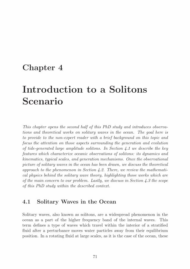
Chapter 4
Introduction to a SolitonsScenario
This chapter opens the second half of this PhD study and introduces observa-tions and theoretical works on solitary waves in the ocean. The goal here isto provide to the non-expert reader with a brief background on this topic andfocus the attention on those aspects surrounding the generation and evolutionof tide-generated large amplitude solitons. In Section 4.1 we describe the keyfeatures which characterize oceanic observations of solitons: its dynamics andkinematics, typical scales, and generation mechanisms. Once the observationalpicture of solitary waves in the ocean has been drawn, we discuss the theoreticalapproach to the phenomenon in Section 4.2. There, we review the mathemati-cal physics behind the solitary wave theory, highlighting those works which areof the main concern to our problem. Lastly, we discuss in Section 4.3 the scopeof this PhD study within the described context.
4.1 Solitary Waves in the Ocean
Solitary waves, also known as solitons, are a widespread phenomenon in theocean as a part of the higher frequency band of the internal waves. Thisterm defines a type of waves which travel within the interior of a stratifiedfluid after a perturbance moves water particles away from their equilibriumposition. In a rotating fluid at large scales, as it is the case of the ocean, these
71
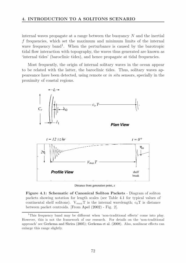
4. INTRODUCTION TO A SOLITONS SCENARIO
internal waves propagate at a range between the buoyancy N and the inertialf frequencies, which set the maximum and minimum limits of the internalwave frequency band1. When the perturbance is caused by the barotropictidal flow interaction with topography, the waves thus generated are known as‘internal tides’ (baroclinic tides), and hence propagate at tidal frequencies.
Most frequently, the origin of internal solitary waves in the ocean appearto be related with the latter, the baroclinic tides. Thus, solitary waves ap-peareance have been detected, using remote or in situ sensors, specially in theproximity of coastal regions.
Figure 4.1: Schematic of Canonical Soliton Packets - Diagram of solitonpackets showing notation for length scales (see Table 4.1 for typical values ofcontinental shelf solitons). VmaxT is the internal wavelength; c0T is distancebetween packet centroids. [From Apel (2002) - Fig. 2].
1This frequency band may be different when ‘non-traditional effects’ come into play.However, this is not the framework of our research. For details on the ‘non-traditionalapproach’ see Gerkema and Shrira (2005); Gerkema et al. (2008). Also, nonlinear effects canenlarge this range slightly.
72
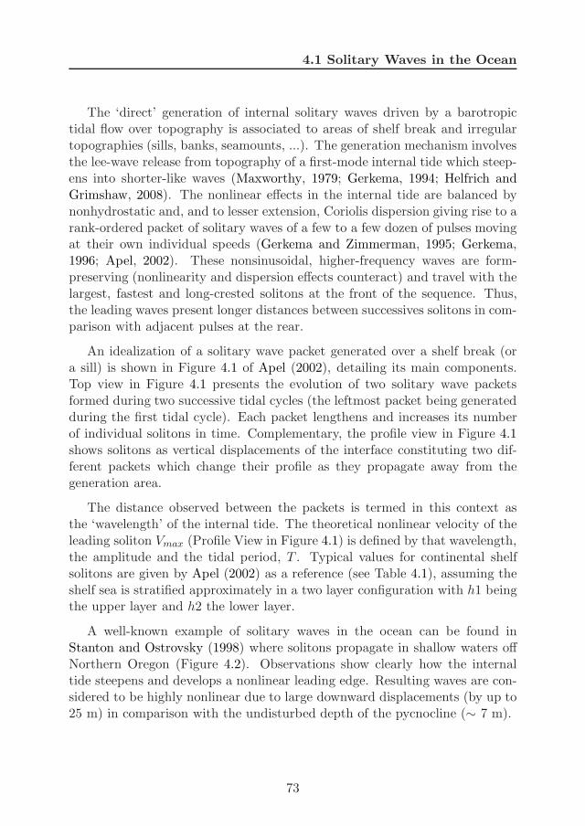
4.1 Solitary Waves in the Ocean
The ‘direct’ generation of internal solitary waves driven by a barotropictidal flow over topography is associated to areas of shelf break and irregulartopographies (sills, banks, seamounts, ...). The generation mechanism involvesthe lee-wave release from topography of a first-mode internal tide which steep-ens into shorter-like waves (Maxworthy, 1979; Gerkema, 1994; Helfrich andGrimshaw, 2008). The nonlinear effects in the internal tide are balanced bynonhydrostatic and, and to lesser extension, Coriolis dispersion giving rise to arank-ordered packet of solitary waves of a few to a few dozen of pulses movingat their own individual speeds (Gerkema and Zimmerman, 1995; Gerkema,1996; Apel, 2002). These nonsinusoidal, higher-frequency waves are form-preserving (nonlinearity and dispersion effects counteract) and travel with thelargest, fastest and long-crested solitons at the front of the sequence. Thus,the leading waves present longer distances between successives solitons in com-parison with adjacent pulses at the rear.
An idealization of a solitary wave packet generated over a shelf break (ora sill) is shown in Figure 4.1 of Apel (2002), detailing its main components.Top view in Figure 4.1 presents the evolution of two solitary wave packetsformed during two successive tidal cycles (the leftmost packet being generatedduring the first tidal cycle). Each packet lengthens and increases its numberof individual solitons in time. Complementary, the profile view in Figure 4.1shows solitons as vertical displacements of the interface constituting two dif-ferent packets which change their profile as they propagate away from thegeneration area.
The distance observed between the packets is termed in this context asthe ‘wavelength’ of the internal tide. The theoretical nonlinear velocity of theleading soliton Vmax (Profile View in Figure 4.1) is defined by that wavelength,the amplitude and the tidal period, T . Typical values for continental shelfsolitons are given by Apel (2002) as a reference (see Table 4.1), assuming theshelf sea is stratified approximately in a two layer configuration with h1 beingthe upper layer and h2 the lower layer.
A well-known example of solitary waves in the ocean can be found inStanton and Ostrovsky (1998) where solitons propagate in shallow waters offNorthern Oregon (Figure 4.2). Observations show clearly how the internaltide steepens and develops a nonlinear leading edge. Resulting waves are con-sidered to be highly nonlinear due to large downward displacements (by up to25 m) in comparison with the undisturbed depth of the pycnocline (∼ 7 m).
73
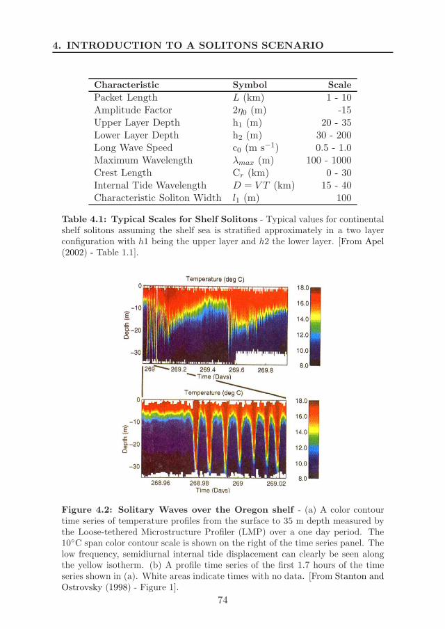
4. INTRODUCTION TO A SOLITONS SCENARIO
Characteristic Symbol Scale
Packet Length L (km) 1 - 10Amplitude Factor 2η0 (m) -15Upper Layer Depth h1 (m) 20 - 35Lower Layer Depth h2 (m) 30 - 200Long Wave Speed c0 (m s−1) 0.5 - 1.0Maximum Wavelength λmax (m) 100 - 1000Crest Length Cr (km) 0 - 30Internal Tide Wavelength D = V T (km) 15 - 40Characteristic Soliton Width l1 (m) 100
Table 4.1: Typical Scales for Shelf Solitons - Typical values for continentalshelf solitons assuming the shelf sea is stratified approximately in a two layerconfiguration with h1 being the upper layer and h2 the lower layer. [From Apel(2002) - Table 1.1].
Figure 4.2: Solitary Waves over the Oregon shelf - (a) A color contourtime series of temperature profiles from the surface to 35 m depth measured bythe Loose-tethered Microstructure Profiler (LMP) over a one day period. The10C span color contour scale is shown on the right of the time series panel. Thelow frequency, semidiurnal internal tide displacement can clearly be seen alongthe yellow isotherm. (b) A profile time series of the first 1.7 hours of the timeseries shown in (a). White areas indicate times with no data. [From Stanton andOstrovsky (1998) - Figure 1].
74
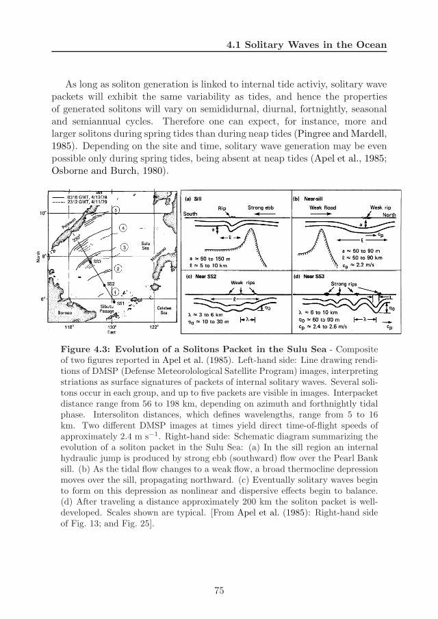
4.1 Solitary Waves in the Ocean
As long as soliton generation is linked to internal tide activiy, solitary wavepackets will exhibit the same variability as tides, and hence the propertiesof generated solitons will vary on semididurnal, diurnal, fortnightly, seasonaland semiannual cycles. Therefore one can expect, for instance, more andlarger solitons during spring tides than during neap tides (Pingree and Mardell,1985). Depending on the site and time, solitary wave generation may be evenpossible only during spring tides, being absent at neap tides (Apel et al., 1985;Osborne and Burch, 1980).
Figure 4.3: Evolution of a Solitons Packet in the Sulu Sea - Compositeof two figures reported in Apel et al. (1985). Left-hand side: Line drawing rendi-tions of DMSP (Defense Meteorolological Satellite Program) images, interpretingstriations as surface signatures of packets of internal solitary waves. Several soli-tons occur in each group, and up to five packets are visible in images. Interpacketdistance range from 56 to 198 km, depending on azimuth and forthnightly tidalphase. Intersoliton distances, which defines wavelengths, range from 5 to 16km. Two different DMSP images at times yield direct time-of-flight speeds ofapproximately 2.4 m s−1. Right-hand side: Schematic diagram summarizing theevolution of a soliton packet in the Sulu Sea: (a) In the sill region an internalhydraulic jump is produced by strong ebb (southward) flow over the Pearl Banksill. (b) As the tidal flow changes to a weak flow, a broad thermocline depressionmoves over the sill, propagating northward. (c) Eventually solitary waves beginto form on this depression as nonlinear and dispersive effects begin to balance.(d) After traveling a distance approximately 200 km the soliton packet is well-developed. Scales shown are typical. [From Apel et al. (1985): Right-hand sideof Fig. 13; and Fig. 25].
75

4. INTRODUCTION TO A SOLITONS SCENARIO
An illustrative case of large-amplitude solitons generated from a sill occurin the Sulu Sea (Apel et al., 1985; Liu et al., 1985). The study area is shownin the left-hand side of Figure 4.3. The mechanism consists on the release of alow-mode internal tide from the Pearl Bank sill (Figure 4.3 - Right-hand side:a - b). Subsequently, as the internal tide propagates nonlinear steepening anddispersive effects come into play leading to the appearance of solitary wavesdistributed into packets separated by tidal cycles (Figure 4.3 - Right-handside: c - d).
The generation mechanism over a shelf break and over a shallow promon-tory (sills, banks, seamounts, ...) is similar; however, solitons propagatingoceanward evolve differently than those traveling shoreward since the formerare generally out of the area controlled by bathymetry. Hence, solitary wavespropagating on the shelf, where the pycnocline depth shoals and the waterdepth diminishes, are conditioned by bottom friction effects. This leads torefraction of the waves, driving the packet crests along isobaths and decreas-ing their amplitudes, speeds and wavelengths, independently from whereversolitons were generated. A clear example of wave refraction of solitons whenwater depth shoals can be found in Zeng and Alpers (2004) for solitary wavestraveling to shallow waters, afresh in the Sulu Sea (Figure 4.4).
Nevertheless, solitary wave packets have been also observed traveling ocean-ward far away from shelf breaks and promotory areas (e.g. solitons in the Bayof Biscay (Gerkema, 2001; New and da Silva, 2002). These solitons respond toa different generation mechanism. Then, we need to consider that internal tidalenergy may radiate away either horizontally as interfacial waves in the ther-mocline (mechanism explained above and termed ‘direct generation’) and/orvertically as ‘beams’ into the stratified continuum below (mechanism known as‘local generation’) (New, 1988, 1990; New and Pingree, 1992; Gerkema, 2001;Akylas et al., 2007; da Silva et al., 2007; Da Silva and New, 2009). These beamsemanate from critical topographies where bottom slope matches the slope ofthe beam paths and travel at an angle to the vertical into the deep ocean.After reflection from the seafloor, scattering of these beams at the base of thethermocline induces the generation of internal solitary waves propagating atlong distances from the shelf break or promontory which caused the initialbeam of internal tidal energy (New, 1990; Gerkema, 2001; Da Silva and New,2009). Other possible mechanism of soliton generation include shear-flow in-stability just up-current of the break/sill (Farmer and Armi, 1999), upstreamblocking (Lee and Beardsley, 1974), transcritical generation (Grimshaw, 1986;
76
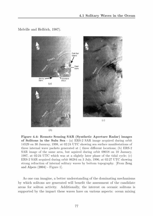
4.1 Solitary Waves in the Ocean
Melville and Helfrich, 1987).
Figure 4.4: Remote Sensing SAR (Synthetic Aperture Radar) imagesof Solitons in the Sulu Sea - (a) ERS-2 SAR image acquired during orbit14529 on 30 Januray, 1998, at 02:24 UTC showing sea surface manifestations ofthree internal wave packets generated at ( three different locations; (b) ERS-2SAR image of the same area, but aquired during orbit 09018 on 10 January,1997, at 02:24 UTC which was at a slightly later phase of the tidal cycle; (c)ERS-2 SAR acquired during orbit 06284 on 3 July, 1996, at 02:27 UTC showingstrong refraction of internal solitary waves by bottom topography. [From Zengand Alpers (2004) - Figure 1].
As one can imagine, a better understanding of the dominating mechanismsby which solitons are generated will benefit the assessment of the candidateareas for soliton activity. Additionally, the interest on oceanic solitons issupported by the impact these waves have on various aspects: ocean mixing
77
4. INTRODUCTION TO A SOLITONS SCENARIO
and biological productivity (Sandstrom and Elliott, 1984; Pinkel, 2000; Sangraet al., 2001; Moum et al., 2003; Macias et al., 2006), water acoustics (Tiemannet al., 2001), sediment transport (Sandstrom and Elliott, 1984; Bogucki et al.,1997; Butman et al., 2006), oil platforms (Osborne and Burch, 1980), etc.The uncertainty about the relative importance of each generating mechanismworlwide leads to the topic of oceanic solitons still represents a challengingfieldwork. Fine reviews of the existing empirical and theoretical backgroundon solitons can be found in Ostrovsky and Stepanyants (1989); Grimshaw et al.(1998); Apel (2002); Apel et al. (2006); Helfrich and Melville (2006).
The seed for next section is linked to the earliest scientific report describingthe surface manifestation of a solitary wave, which was made by J. ScottRussell in 1838 on a propagating and unchanging single hump in a Scottishcanal (Russell, 1838b,a). Half a century later, Korteweg and de Vries providedfor the first time a theoretical explanation to this important phenomenonin the field of mathematical physics (Korteweg and de Vries, 1895). Thatwork opened an entire research line on the study of soliton properties from atheoretical point of view whose interest persists in time. In the following wefocus on introducing the solitary wave theory which is of the main concern forthe background of this PhD research.
4.2 A Mathematical Approach to Solitons
To set the scope of the present thesis, we first discuss soliton wave theory basedon the applications of the quadratic Korteweg-de Vries equation (KdV) andits extended cubic version (eKdV), which describe the dominant wave char-acteristics and evolution of solitons under weakly (KdV) and more stronglynonlinear conditions (eKdV), respectively, given an initial profile. Theoreticalmodels are traditionally built up starting from the most simplified situationpossible, which gets more comprehensive by including new elements in model-ing the process as long as a previous scenario is understood. On solitary wavetheory, it is not surprising that KdV-type models have become the classical ap-proach to describe nonlinear dispersive waves. They have been widely used inthe literature and show good aggreement with dominant relationships betweenphase speed, amplitude and wavelength scales in comparison with reported ob-servations of oceanic solitons (Osborne and Burch, 1980; Pingree and Mardell,1985; Ostrovsky and Stepanyants, 1989; Stanton and Ostrovsky, 1998; Xu andYin, 2012). Additionally, they permit modeling the phenomenon of interest
78
4.2 A Mathematical Approach to Solitons
with a reduced set of equations. However, not all quantitative features arefully well captured.
The Korteweg-de Vries (KdV) equation is a quadratic nonlinear modelwhich admits form-preserving solitary wave solutions travelling in one dimen-sion and based on a balance between nonlinearity and dispersive effects. Forsimplicity, here we discuss the KdV equation in terms of a two-layer fluidwith a rigid lid at the surface, even bottom and no mean flow (Djordjevic andRedekopp, 1978; Kakutani and Yamasaki, 1978), following
∂η
∂t+ c0
∂η
∂x+ αη
∂η
∂x+ β
∂3η
∂x3= 0 (4.1)
where t is time; x is the spatial variable in the direction of wave propaga-tion; h1 (h2) is the thickness of the upper (lower) layer; g is the gravitationalacceleration; η(x, t) is the interfacial displacement from its rest level; and α,β and c0 are the so-called environmental coefficients of the medium describingnonlinearity, dispersion and long-wavelength phase speed which read
c20 = ∆ρg
h1h2
h1 + h2, α =
3
2
h1 − h2
h1h2c0, β =
1
6h1h2c0, (4.2)
with ∆ρ = (ρ2 − ρ1)/ρ2. Additionally, relative differences in density be-tween the two layers (∆ρ) are assumed to be small (Boussinesq approxima-tion), what holds in the ocean with typical values of the order 10−3.
This KdV equation is applicable in shallow waters to stratified fluids wheretwo main assumptions are taken: 1) The interfacial displacement is muchsmaller (but of finite amplitude) than the depth of either layer (i. e., weaknonlinearity); and, 2) waves are long (but of finite length) in comparisonwith the fluid depth (i. e., weak nonhydrostatic dispersion). Thus, the KdVequation is scaled by the small parameters α = a/H and β = (H/l)2 in sucha form that both are small and of comparable order (β = O(α) ≪ 1); takinga as a measure of the wave amplitude, l as the length scale of the wave, andH as the intrinsic vertical scale. The limit in which waves are infinitesimal(α → 0 leads to linearity) and of infinite length (β → 0 leads to hydrostacy)reduces 4.1 to ∂η
∂t + c0∂η∂x , which simply describes rightward travelling waves.
Wherever waves are assumed to be small but of finite amplitude and long
79

4. INTRODUCTION TO A SOLITONS SCENARIO
but of finite wavelength, parameters α and β take values different from zeroto include, respectively, nonlinear and nonhydrostatic dispersive effects in theKdV evolution equation.
The prototypical analytical solution to the KdV equation for a single solitonis the hyperbolic secant profile, which reads
η(x, t) = η0sech2(x − ct
λ
)(4.3)
where c is the nonlinear phase speed derived from KdV theory and relatedto the linear phase speed c0 and amplitude; and λ is the characteristic widthof the soliton, being related to the amplitude of the displacement η0 and theenvironmental cofficients:
c = c0 +αη0
3, λ2 =
12β
αη0(4.4)
As λ2 must be positive, for a thin upper layer with h1 < h2 we have thatα < 0, what results in downgoing displacements of the interface between thelayers (η < 0). On the other hand, if the lower layer shoals in such a mannerthat h2 < h1, then solitons reverse to upgoing displacements (α < 0, η > 0).At the configuration in which h1 = h2, the quadratic nonlinear coefficient αvanishes and a higher-order (cubic) nonlinear coefficient must be included inthe KdV equation (Djordjevic and Redekopp, 1978; Kakutani and Yamasaki,1978), leading to its extended version (eKdV):
∂η
∂t+ (c0 + αη + α1η
2)∂η
∂x+ β
∂3η
∂x3= 0 (4.5)
where the coefficient α1, absent in the Kdv equation (4.1), is the abovementioned cubic nonlinear coefficient
α1 =3c0
(h1h2)2
[78(h1 − h2)
2 −(h3
2 + h31
h1 + h2
)](4.6)
80
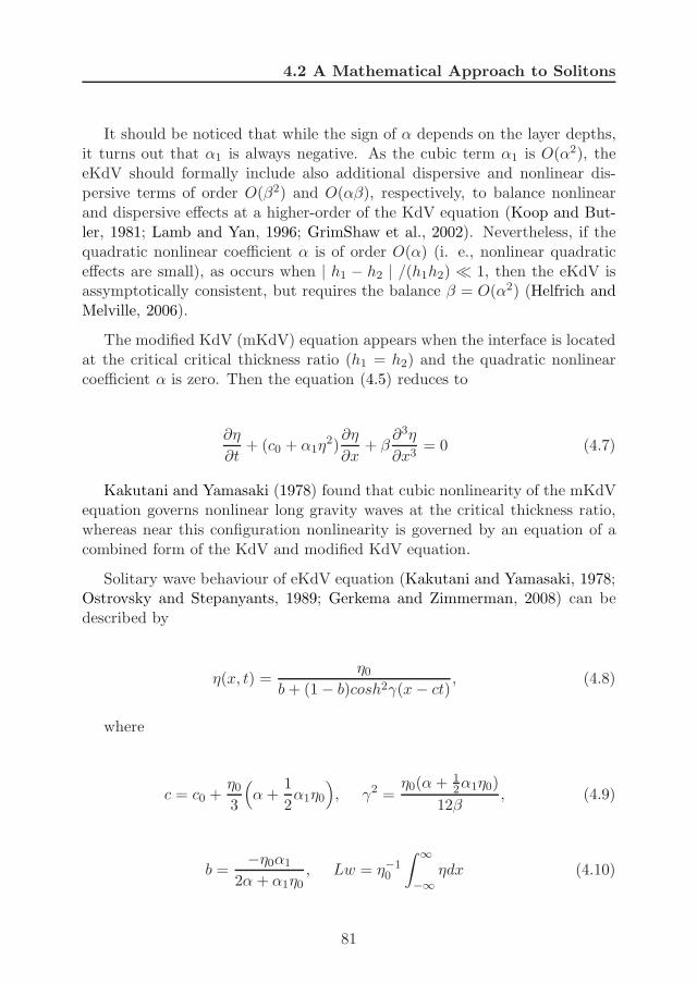
4.2 A Mathematical Approach to Solitons
It should be noticed that while the sign of α depends on the layer depths,it turns out that α1 is always negative. As the cubic term α1 is O(α2), theeKdV should formally include also additional dispersive and nonlinear dis-persive terms of order O(β2) and O(αβ), respectively, to balance nonlinearand dispersive effects at a higher-order of the KdV equation (Koop and But-ler, 1981; Lamb and Yan, 1996; GrimShaw et al., 2002). Nevertheless, if thequadratic nonlinear coefficient α is of order O(α) (i. e., nonlinear quadraticeffects are small), as occurs when | h1 − h2 | /(h1h2) ≪ 1, then the eKdV isassymptotically consistent, but requires the balance β = O(α2) (Helfrich andMelville, 2006).
The modified KdV (mKdV) equation appears when the interface is locatedat the critical critical thickness ratio (h1 = h2) and the quadratic nonlinearcoefficient α is zero. Then the equation (4.5) reduces to
∂η
∂t+ (c0 + α1η
2)∂η
∂x+ β
∂3η
∂x3= 0 (4.7)
Kakutani and Yamasaki (1978) found that cubic nonlinearity of the mKdVequation governs nonlinear long gravity waves at the critical thickness ratio,whereas near this configuration nonlinearity is governed by an equation of acombined form of the KdV and modified KdV equation.
Solitary wave behaviour of eKdV equation (Kakutani and Yamasaki, 1978;Ostrovsky and Stepanyants, 1989; Gerkema and Zimmerman, 2008) can bedescribed by
η(x, t) =η0
b + (1 − b)cosh2γ(x − ct), (4.8)
where
c = c0 +η0
3
(α +
1
2α1η0
), γ2 =
η0(α + 12α1η0)
12β, (4.9)
b =−η0α1
2α + α1η0, Lw = η−1
0
∫∞
−∞
ηdx (4.10)
81
4. INTRODUCTION TO A SOLITONS SCENARIO
with η0 being a measure of the maximum amplitude of the soliton; Lw thecharacteristic wave-width; c, the nonlinear phase speed derived from eKdVtheory; and, b and γ parameters defining the system.
Figure 4.5 shows eKdV solitary waves approaching its maximum amplitudeand becoming flat-topped, a radical departure from the classical KdV solitonwhich has no formal mathematical limit to its amplitude.
Figure 4.5: Solitary wave solutions of the eKdV equation - Examples ofsolitary wave solutions of the eKdV equation (Equation 6) for the arbitrary choiceof the parameters β = α = α1. As the maximum wave amplitude increases, thewaves eventually broaden and develop a flat crest at the maximum amplitudeη0max
= 1. [From Helfrich and Melville (2006) - Figure 4].
As previously pointed out, within the framework of the two-layer model,α1 is always negative (4.6). However, for more general stratifications andbackground shear flows the cubic nonlinear coefficient may be either negativeor positive. In the latter case, soliton solutions of both positive and negativepolarities may exist regardless of the sign of α (Grimshaw et al., 1997, 2004).
Cubic KdV, though including higher nonlinearities, is still based on anexpansion of a small parameter (α = a/H) and so is still subject to the as-sumption of weak nonlinearity. A useful and well-known radical departurefrom the weakly nonlinear two-layer KdV model was derived by Miyata (1985,1988) and Choi and Camassa (1999). The result of their work was an equiva-
82

4.2 A Mathematical Approach to Solitons
lent set of bi-directional wave equations with full nonlinearity, α = O(1) andfirst-order weakly dispersive effects, β ≪ 1.
Figure 4.6: Comparison of KdV and MCC theories - Comparison ofsolitary wave properties from the two-layer KdV (red), eKdV (blue), and MCC(orange) theories. The top row shows the wave speed c vs. amplitude η0; andthe bottom row shows the wavelength (here read characteristic wave-width of thesoliton) Lw vs. η0. The comparison is done for the two stratifications h1/h2 =1/4 (left column) and h1/h2 = 2/3 (right column). For both the eKdV and MCCwaves the maximum wave amplitude corresponds to the end of the speed curves.[From Helfrich and Melville (2006) - Figure 5].
Helfrich and Melville (2006) highlighted with Figure 4.6 the deviationamong the weakly nonlinear KdV, the more strongly nonlinear eKdV and thefully nonlinear Miyata-Choi-Camassa (MCC) models. The amplitude depen-
83
4. INTRODUCTION TO A SOLITONS SCENARIO
dence of the wave speed c and characteristic wave-width Lw1 from the threemodels is shown for two different layer-thickness (h1/h2 = 1/4 and h1/h2 =2/3) in a two-fluid layer system.
Remarkable differences arise when comparing results from the weakly non-linear KdV and the strongly nonlinear eKdV and MCC models, for both c andLw, even for relatively small amplitudes. The solitary wave solutions of theeKdV and MCC equations increase its phase speed c with growing amplitudeuntil they start to slow as they approach its maximum η0max (Figure 4.6 -top row). On the contrary, KdV solutions show the phase speed increasinglinearly with amplitude. Additionally, it also worth noting that the maximumwave amplitude for both the eKdV and MCC waves corresponds to the end ofthe speed curves (what it does not occur with KdV solitons).
As previously shown in Figure 4.5 for eKdV solitary waves, its characteristicwave-width becomes narrower as they grow (increasing η0) to lately broadenwhen the upper limit is approached (η0max). This behaviour is also exhibitedby the MCC theory (Figure 4.6 - bottom row); and, unlike classical KdVsolitary waves whose wave-width gets narrower as they become larger until itsmaximum amplitude.
On a whole, comparison of the wave shapes and properties between theeKdV and MCC theories agree quite well for 0.4 < h1/(h1 + h2) < 0.6, wherethe scaling requirements of eKdV are reasonably met (Helfrich and Melville,2006). Outside this range, differences among the two theories start to grow(see Figure 4.6 - left column, bottom row).
As we have described, the Korteweg-de Vries (KdV) equation and its ex-tended version (eKdV) with no forcing terms included, provide an appropiatemathematical tool for studying the evolution of a given initial profile underweakly nonlinear (KdV and eKdV) conditions. To go to strongly nonlinearsettings, MCC-type of equations need to be used. But for these, no model ex-ists that includes a forcing mechanism. It is the principal goal of the followingchapters to extend MCC to include the mechanism of forcing by barotropictides over topography.
Throughout the next section, the basis and scope of the present thesis arediscussed.
1For KdV solitary waves Lw = 2γ−1.
84
4.3 Scope of the Study
4.3 Scope of the Study
It is now our interest to include a forcing element in the system to reproducethe generation and evolution of fully nonlinear weakly nonhydrostatic solitonsin a rotating ocean through the disintegration of a low-mode internal tidereleased from topography interaction. However, tide-topography interactiongives rises to waves propagating in two directions (left- and rightward of thetopographic obstacle) and the KdV theory describes waves travelling in oneunique direction. Additionally, Coriolis dispersion needs to be included, whichis not accounted for in (e)KdV. Hence, the KdV-type models are not suitableto be generalized for including this forcing mechanism. We shall use a differentstarting point from that of the Korteweg-de Vries equation. The framework ofour generation model will be the Euler and continuity equations, which are notunidirectionally restricted. In the following we discuss the main assumptionsand approximations taken in our study, its validity and, therefore, the scopeof the resulting generation model. However, for clarity, we will recall theassumptions and approximations again in Chapter 5.
We choose the simplest possible configuration, widely used in the literaturefor analogous models: a two-fluid layer system in which each layer consists ofan incompressible, homogeneous and inviscid fluid. This configuration sup-ports our study as it can describe the first mode of a generated internal tide(Gerkema, 1994); and we are concerned with the generation of internal solitarywaves by disintegration of a low-mode internal tide (the generation of solitonsby internal tide beams is here discarded).
The waves will be taken to propagate in the x direction. With rotation,motion in the transverse y direction will occur; however, a further simplifica-tion will consist in omiting transverse dependences (hence we consider planewaves). Otherwise, derivation of the model would have to face with morecomplicated equations that may not outweigh the improvement in the results.
Relative differences in density within the ocean are extremely small (typicalvalues are of order 10−3), and so in terms of a two-layer system we can applythe Boussinesq approximation (∆ρ = (ρ2 − ρ1)/ρ2 ≪ 1). Additionally, weexclude any motion at the upper surface with a rigid lid, what enable us toreduce the set of evolution equations.
The forcing for internal tide generation consists of an oscillating non-flatbottom mimicking a barotropic tidal flow over topography. Subsequently,
85

4. INTRODUCTION TO A SOLITONS SCENARIO
solitons are generated by strongly nonlinear disintegration of the first-modeof the internal tide, with waves taken to be long in comparison with the totalfluid depth (weakly nonhydrostatic dispersive waves).
Dispersion due to the Earth’s rotation cannot be neglected, as the wave-length of the internal tides are of the order of the ‘internal Rossby radius ofdeformation’ (c0/f). We therefore include these effects by using the so-calledf -plane approximation. Hence, on a whole, our system includes dispersiveeffects due to weakly nonhydrostatic and Coriolis dispersion.
Therefore, our theoretical approach allows us to study the generation andevolution of nonlinear interfacial waves in the limit of fully nonlinear weaklynonhydrostatic long waves. The strongly nonlinearities arise via disintegrationof a low-mode internal tide released from topography interaction in a rotatingocean. Dispersive effects include weakly nonhydrostatic and Coriolis disper-sion (due to the Earth’s rotation). In the absence of a mechanism for thegeneration of the internal tide and neglecting Earth’s rotation effects, our setof equations reduces to equivalent Choi & Camassa equations.
The interpretation of a mathematical model like the one we are dealing hereis always made easier if analytical solutions are feasible; however, even whenanalytical solving is doable, sometimes it is cumbersome because equationsbecome extremely complicated and puzzle the physics behind the phenomenon.In our case, numerical solving represents a more suitable treatment to explorethe theoretical model and its behaviour.
86
Chapter 5
A Model for the Generationof Strongly Nonlinear,Weakly NonhydrostaticInterfacial Waves1
5.1 Outline
In this chapter we derive a new two-fluid layer model consisting of a set offorced rotation-modified Boussinesq equations for studying the generation andevolution of strongly nonlinear weakly nonhydrostatic dispersive interfacialwaves. The forcing for internal tide generation is due to tide-topographyinteraction (an oscillating non-flat bottom mimicking a barotropic tidal flowover topography). Solitons are generated by disintegration of the first-modeof the internal tide. Dispersive effects include weakly nonhydrostatic andCoriolis dispersion (due to the Earth’s rotation). The model equations arederived in Sections 5.2 to 5.5. The basic equations of Section 5.2 are scaledin Sections 5.3 and vertically integrated over the layers in Section 5.4. Up tothis point, the resulting equations are exact but do not form a closed set. Theset is closed in Section 5.5 by making an expansion in the small parameter
1Aguiar -Gonzalez B., Gerkema T. A Model for the Generation of Strongly Nonlinear,Weakly Nonhydrostatic Interfacial Waves. In Preparation to be Submitted to an International
refereed Journal
87

5. A GENERATION MODEL OF SOLITONS
δ (measuring the strength of non-hydrostaticity). Readers who are primarilyinterested in the results may want to skip Sections 5.3-5.5. The forcing isintroduced in Section 5.6 and the set of equations is rearranged to put it in aform convenient for numerical solving. A numerical algorithm for solving thefully nonlinear model is developed and described in Section 5.7. Application ofthe numerical scheme requires further rearranging, the end-result of which ispresented in Section 5.7.3. The model turns out equivalent to Choi & Camassa(CC) equations plus additional terms which provide the forcing and rotationeffects to the system. Numerical experiments for various regimes are discussedin Chapter 6.
5.2 Preliminaries
We start from the continuity and Euler equations and consider a two-fluidlayer configuration in which each layer is composed of a homogeneous, inviscid,incompressible fluid, applying the Boussinesq approximation. We also assumeuniformity in one of the horizontal directions, taking ∂/∂y = 0. Hence, thecontinuity and momentum equations read
∂ui
∂x+
∂wi
∂z= 0 (5.1)
ρ(∂ui
∂t+ ui
∂ui
∂x+ wi
∂ui
∂z− fvi
)= −∂pi
∂x(5.2)
∂vi
∂t+ ui
∂vi
∂x+ wi
∂vi
∂z+ fui = 0 (5.3)
ρ(∂wi
∂t+ ui
∂wi
∂x+ wi
∂wi
∂z
)= −∂pi
∂z− ρig (5.4)
where ρi is density, (ui,vi,wi) are the velocity components in Cartesian coordi-nates, pi is pressure, g the gravitational accelaration, f the Coriolis parameter(f = 2Ωsinφ, at latitude φ) and ρ the mean density. The subscript i = 1(i = 2) refers to the upper (lower) layer and a stable stratification, ρ1 < ρ2, isassumed.
Boundaries are defined at the surface, taken to be a rigid lid, which islocated at z = H1, and at the bottom, located at z = −H2+H(x, t). The time-dependence of the bottom will later be specified as a horizontal oscillation,mimicking a barotropic tidal flow over topography, the forcing mechanismfor internal tides. However, the two are not exactly equivalent, since the
88
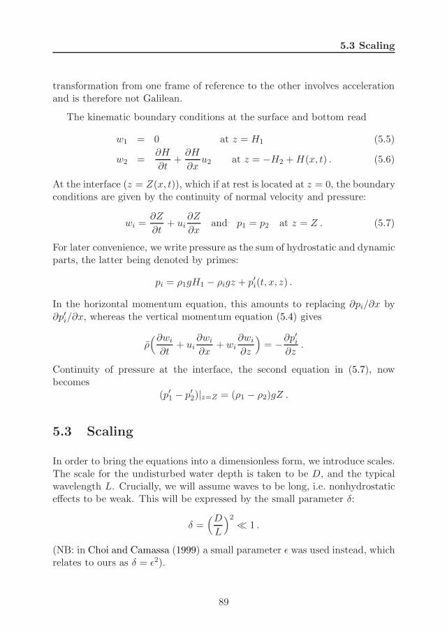
5.3 Scaling
transformation from one frame of reference to the other involves accelerationand is therefore not Galilean.
The kinematic boundary conditions at the surface and bottom read
w1 = 0 at z = H1 (5.5)
w2 =∂H
∂t+
∂H
∂xu2 at z = −H2 + H(x, t) . (5.6)
At the interface (z = Z(x, t)), which if at rest is located at z = 0, the boundaryconditions are given by the continuity of normal velocity and pressure:
wi =∂Z
∂t+ ui
∂Z
∂xand p1 = p2 at z = Z . (5.7)
For later convenience, we write pressure as the sum of hydrostatic and dynamicparts, the latter being denoted by primes:
pi = ρ1gH1 − ρigz + p′i(t, x, z) .
In the horizontal momentum equation, this amounts to replacing ∂pi/∂x by∂p′i/∂x, whereas the vertical momentum equation (5.4) gives
ρ(∂wi
∂t+ ui
∂wi
∂x+ wi
∂wi
∂z
)= −∂p′i
∂z.
Continuity of pressure at the interface, the second equation in (5.7), nowbecomes
(p′1 − p′2)|z=Z = (ρ1 − ρ2)gZ .
5.3 Scaling
In order to bring the equations into a dimensionless form, we introduce scales.The scale for the undisturbed water depth is taken to be D, and the typicalwavelength L. Crucially, we will assume waves to be long, i.e. nonhydrostaticeffects to be weak. This will be expressed by the small parameter δ:
δ =(D
L
)2≪ 1 .
(NB: in Choi and Camassa (1999) a small parameter ǫ was used instead, whichrelates to ours as δ = ǫ2).
89
5. A GENERATION MODEL OF SOLITONS
Since we allow waves to have large amplitudes (i.e. being strongly nonlin-ear), we may take horizontal velocities to scale with c = (g′D)1/2, where g′ isreduced gravity,
g′ = gρ2 − ρ1
ρ.
c, roughly, is a measure of the linear long-wave phase speed for interfacialwaves. Thus, u and v will be scaled with c. For the interfacial displacementbeing allowed to be large, an appropriate scale of Z is D.
The typical scale of w now follows from the continuity equation as Dc/L.Finally, the scale of pressure follows from assuming a primary balance be-tween the acceleration term ρ∂u/∂t and ∂p/∂x in the horizontal momentumequation.
In summary, then, we can introduce the following dimensionless variables,indicated by asterisks,
x = L x∗, z = D z∗, t = (L/c) t∗,p′i = (ρ c2) p′∗i , ui = c u∗
i , vi = c v∗i , wi = (D/L) c w∗
i .(5.8)
With these scales, the dimensionless continuity and Euler equations yield (forconvenience, we drop the asterisks right away):
∂ui
∂x+
∂wi
∂z= 0 (5.9)
∂ui
∂t+ ui
∂ui
∂x+ w1
∂ui
∂z− µvi = −∂p′i
∂x(5.10)
∂vi
∂t+ ui
∂vi
∂x+ w1
∂vi
∂z+ µui = 0 (5.11)
δ(∂wi
∂t+ ui
∂wi
∂x+ wi
∂wi
∂z
)= −∂p′i
∂z. (5.12)
Here µ is the scaled Coriolis parameter, µ = fL/c. Furthermore we introducethe dimensionless quantities ζ, hi, and h via (Z,H1,H2,D) = (ζ, h1, h2, h), sothat the scaled form of the boundary conditions is
w1 = 0 at z = h1 (5.13)
w2 =∂h
∂t+ u2
∂h
∂xat z = −h2 + h(x, t) (5.14)
wi =∂ζ
∂t+ ui
∂ζ
∂xat z = ζ(x, t) (5.15)
p′2 − p′1 = ζ at z = ζ(x, t) . (5.16)
90

5.4 Vertically Integrated Equations
5.4 Vertically Integrated Equations
From here on we follow a procedure analagous to that of Choi & Camassa(1999), i.e. we vertically integrate the equations over their layers, and thenconsider subsequently the orders δ0 and δ1 in order to obtain a closed set forthe weakly nonhydrostatic equations.
The layer-mean f1 of a function f1(x, z, t) for the upper layer is defined as
f1(x, t) =1
η1
∫ h1
ζdz f1(x, z, t) , η1 = h1 − ζ (5.17)
and for the lower layer as
f2(x, t) =1
η2
∫ ζ
−h2+hdz f2(x, z, t) , η2 = h2 − h + ζ . (5.18)
Here, ηi represents the thickness of the layer (depending on the interfacialdisplacement ζ). Notice that the boundaries contain a dependence on t and xvia ζ(t, x) and h(t, x).
5.4.1 Upper Fluid-Layer
Vertical integration of the continuity equation (5.9), from the interface (ζ) tothe surface (h1) yields
∂η1
∂t+
∂(η1u1)
∂x= 0 . (5.19)
Here we used the theorem for derivatives of integrals with variable bound-aries (see Appendix B):
∂
∂x
∫ B(x)
A(x)f(x, z) dz =
∫ B(x)
A(x)
∂f(x, z)
∂xdz+f(x,B(x))
dB(x)
dx−f(x,A(x))
dA(x)
dx.
The vertical integration of the Euler equation (5.10) involves the followingsteps. For the acceleration term we get
∫ h1
ζdz
∂u1
∂t=
∂
∂t
∫ h1
ζdz u1 + u1|z=ζ
∂ζ
∂t=
∂(η1u1)
∂t+ u1|z=ζ
∂ζ
∂t.
91
5. A GENERATION MODEL OF SOLITONS
The vertical integration of the nonlinear terms, which can be rewritten (u21)x+
(w1u1)z, yields
∫ h1
ζdz [(u2
1)x + (w1u1)z ] =∂
∂x
∫ h1
ζdz u2
1 + u21
∣∣∣z=ζ
∂ζ
∂x+ (w1u1)|h1
ζ
=∂η1u2
1
∂x− ∂ζ
∂tu1|z=ζ
The vertically integrated first horizontal momentum equation becomes
∂(η1u1)
∂t+
∂(η1u1u1)
∂x− µη1v1 = −η1
(∂p′1∂x
). (5.20)
The other horizontal momentum equation is treated similarly. The non-linear terms can be rewritten as (uv)x + (wv)z , and become after verticalintegration
∫ h1
ζdz (u1v1)x + (w1v1)z =
∂
∂x
∫ h1
ζdz u1v1 + (u1v1)|z=ζ
∂ζ
∂x− (w1v1)|z=ζ
=∂
∂x(η1u1v1) −
∂ζ
∂tv1|z=ζ
Then, the vertically integrated second horizontal momentum equation gives
∂(η1v1)
∂t+
∂(η1u1v1)
∂x+ µη1u1 = 0 . (5.21)
5.4.2 Lower Fluid-Layer
For the lower layer one proceeds similarly, except that now both boundaries arevariable when one integrates vertically from the interface (ζ) to the bottom(−h2 + h).
First, the vertical integration of the continuity equation yields
∫ ζ
−h2+hdz
∂u2
∂x=
∂
∂x
∫ ζ
−h2+hdz u2 − u2|z=ζ
∂ζ
∂x+ u2|z=−h2+h
∂h
∂x
92
5.4 Vertically Integrated Equations
and
w2|ζ−h2+h =∂ζ
∂t+ u2|z=ζ
∂ζ
∂x− ∂h
∂t− u2|z=−h2+h
∂h
∂xCombined, this yields
∂η2
∂t+
∂(η2u2)
∂x= 0 . (5.22)
The vertical integration of the Euler equation (5.10) involves the followingsteps. For the acceleration term we get
∫ ζ
−h2+hdz
∂u2
∂t=
∂
∂t
∫ ζ
−h2+hdz u2 − u2|z=ζ
∂ζ
∂t+ u2|z=−h2+h
∂h
∂t
=∂(η2u2)
∂t− u2|z=ζ
∂ζ
∂t+ u2|z=−h2+h
∂h
∂t.
The vertical integration of the nonlinear terms, which can be rewritten(u2
2)x + (w2u2)z, yields
∫ ζ
−h2+hdz [(u2
2)x + (w2u2)z]
=∂
∂x
∫ ζ
−h2+hdz u2
2 − u22
∣∣∣z=ζ
∂ζ
∂x+ u2
2
∣∣∣z=−h2+h
∂h
∂x+ (w2u2)|ζ−h2+h
=∂η2u
22
∂x− u2
2
∣∣∣z=ζ
∂ζ
∂x+ u2
2
∣∣∣z=−h2+h
∂h
∂x+(∂ζ
∂t+ u2
∂ζ
∂x
)u2|z=ζ
−(∂h
∂t+ u2
∂h
∂x
)u2|z=−h2+h
=∂η2u2
2
∂x+
∂ζ
∂tu2|z=ζ −
∂h
∂tu2|z=−h2+h
The vertically integrated first horizontal momentum equation becomes
∂(η2u2)
∂t+
∂(η2u2u2)
∂x− µη2v2 = −η2
(∂p′2∂x
). (5.23)
93
5. A GENERATION MODEL OF SOLITONS
The other horizontal momentum equation is treated similarly. The accelera-tion term gives
∫ ζ
−h2+hdz
∂v2
∂t=
∂(η2v2)
∂t− v2|z=ζ
∂ζ
∂t+ v2|z=−h2+h
∂h
∂t.
The nonlinear terms can be rewritten as (uv)x + (wv)z , and yield aftervertical integration
∫ ζ
−h2+hdz (u2v2)x + (w2v2)z
=∂
∂x
∫ h1
ζdz u2v2 − (u2v2)|z=ζ
∂ζ
∂x+ (u2v2)|z=−h2+h
∂h
∂x
+(∂ζ
∂t+ u2
∂ζ
∂x
)v2|z=ζ −
(∂h
∂t+ u2
∂h
∂x
)v2|z=−h2+h
=∂
∂x(η2u2v2) +
∂ζ
∂tv2|z=ζ −
∂h
∂tv2|z=−h2+h
Thus, the vertically integrated second horizontal momentum equation gives
∂(η2v2)
∂t+
∂(η2u2v2)
∂x+ µη2u2 = 0 . (5.24)
5.5 Expansion in δ
The six integrated equations (5.19 - 5.24) derived so far, are exact but do notform a closed set. The variables η1, η2 and ζ count as one unknown, but wehave also ui, vi, p′i,x. uiui and uivi. The last two expressions will be castin terms of ui and vi by using the vertical momentum equation, expandedin terms of the small parameter δ. Moreover, continuity of pressure at theinterface is used to connect the pressure in the lower and upper layer. All inall, the six equations are thus modified to contain only six unknowns.
We make a formal expansion of the unknowns as, for example,
ui = ui(0) + δui
(1) + · · ·
94

5.5 Expansion in δ
5.5.1 Lowest Order
The vertical momentum equation reduces to ∂p′i(0)/∂z = 0 neglecting terms of
order δ. At lowest order, (perturbation) pressure is vertically constant in eachlayer. For convenience, we introduce P = p′2
(0), being a function of t and x. Itthen follows from continuity of pressure at the interface, that p′1
(0) = P − ζ.Thus,
(∂p′1∂x
)=
∂P
∂x− ∂ζ
∂x+ O(δ) ,
(∂p′2∂x
)=
∂P
∂x+ O(δ) .
Returning to the original horizontal momentum equations, it is now naturalto assume that the horizontal velocities, too, are independent of z within eachlayer, given the z-independence of pressure. Thus,
uiui = u2i + O(δ) , uivi = uivi + O(δ).
At lowest order, then, the set of integrated equations is closed, in terms of thesix variables ui, vi, ζ and P :
∂(η1u1)
∂t+
∂(η1u21)
∂x− µη1v1 = −η1
(∂P
∂x− ∂ζ
∂x
)+ O(δ) (5.25)
∂(η2u2)
∂t+
∂(η2u22)
∂x− µη2v2 = −η2
∂P
∂x+ O(δ) (5.26)
∂(ηivi)
∂t+
∂(ηiuivi)
∂x+ µηiui = O(δ) (5.27)
∂ηi
∂t+
∂(ηiui)
∂x= 0 . (5.28)
(Notice that the last equation, representing the vertically integrated continuityequations, is exact and involves no approximation in terms of δ.)
We can obtain the lowest-order expressions wi(0) from the continuity equa-
tion
wi(0) = −z
∂ui(0)
∂x+ ci(t, x)
where ci are constants of integration, which are determined by using theboundary conditions at the surface (5.13) and bottom (5.14). For these weget:
w1(0) = (h1 − z)
∂u1(0)
∂x(5.29)
w2(0) = (h − h2 − z)
∂u2(0)
∂x+ D2h (5.30)
95
5. A GENERATION MODEL OF SOLITONS
where the operator Di is defined as ∂/∂t + ui(0)∂/∂x
5.5.2 Next Order
At this order, we include terms of order δ. The key problem is, again, to closethe set of six vertically integrated equations by deriving closed expressions forthe horizontal pressure gradients p′i,x as well as for the contributions of uiui
and uivi in the nonlinear terms.
The latter problem is particularly simple. At order δ, the products containone lowest-order field, which is independent of z, hence
uiui =1
ηi
∫dz u2
i =1
ηi
∫dz (ui
(0) + δui(1) + · · · )2
=1
ηi
∫dz (ui
(0)2 + 2δui(0)ui
(1) + · · · )
= ui(0)2 + 2δui
(0) 1
ηi
∫dz ui
(1) + · · ·
= ui(0)2 + 2δui
(0)ui(1) + · · ·
= (ui(0) + δui
(1) + · · · )2
= u2i + O(δ2)
what leads to
uiui = u2i + O(δ2) , uivi = uivi + O(δ2).
This means that we can write the horizontal momentum equations as
∂(ηiui)
∂t+
∂(ηiu2i )
∂x− µηivi = −ηi
(∂p′i(0) + δ∂p′i
(1)
∂x
)+ O(δ2) (5.31)
∂(ηivi)
∂t+
∂(ηiuivi)
∂x+ µηiui = O(δ2) (5.32)
∂ηi
∂t+
∂(ηiui)
∂x= 0 . (5.33)
96

5.5 Expansion in δ
The remaining problem is to find an expression for p′i(1). Before we enter that
problem, we first simplify the above equations by combining them, using
∂(ηiui)
∂t+
∂(ηiu2i )
∂x= ηi
∂ui
∂t+ ui
∂ηi
∂t+ ηiui
∂ui
∂x+ ui
∂(ηiui)
∂x
= ηi∂ui
∂t+ ηiui
∂ui
∂x(5.34)
and
∂(ηivi)
∂t+
∂(ηiuivi)
∂x= ηi
∂vi
∂t+ vi
∂ηi
∂t+ ηiui
∂vi
∂x+ vi
∂(ηiui)
∂x
= ηi∂vi
∂t+ ηiui
∂vi
∂x. (5.35)
Hence,
∂ui
∂t+ ui
∂ui
∂x− µvi = −
(∂p′i(0) + δ∂p′i
(1)
∂x
)+ O(δ2) (5.36)
∂vi
∂t+ ui
∂vi
∂x+ µui = O(δ2) (5.37)
∂ηi
∂t+
∂(ηiui)
∂x= 0. (5.38)
At order δ, the vertical momentum equations reads
∂wi(0)
∂t+ ui
(0) ∂wi(0)
∂x+ wi
(0) ∂wi(0)
∂z= −∂p′i
(1)
∂z. (5.39)
We now use the lowest order expressions for the velocity components to findan expression for p′i
(1).
5.5.2.1 Pressure in Upper Layer
With the lowest-order expression for the vertical velocity,
w1(0) = (h1 − z)
∂u1(0)
∂x,
97
5. A GENERATION MODEL OF SOLITONS
the left-hand side of (5.39) becomes
(h1 − z)∂2u1
(0)
∂x∂t+ u1
(0)(h1 − z)∂2u1
(0)
∂x2− (h1 − z)
(∂u1(0)
∂x
)2
= (h1 − z)[∂2u1
(0)
∂x∂t+ u1
(0) ∂2u1
(0)
∂x2−(∂u1
(0)
∂x
)2]
≡ (h1 − z)G1 , (5.40)
where we introduced
Gi =∂2ui
(0)
∂x∂t+ ui
(0) ∂2ui
(0)
∂x2−(∂ui
(0)
∂x
)2(5.41)
Hence,
∂p′1(1)
∂z= (z − h1)G1 . (5.42)
Integration now gives
p′1(1) = (z2/2 − h1z)G1 − (ζ2/2 − h1ζ)G1
=1
2
[z(z − 2h1) − ζ(ζ − 2h1)
]G1 (5.43)
In the first equality, we used the freedom to add a constant of integration (infact, a function of x and t), to add terms such that pressure is zero at theinterface1. Taking the derivative to x,
∂p′1(1)
∂x= (h1 − ζ)
∂ζ
∂xG1 +
1
2
[z(z − 2h1) − ζ(ζ − 2h1)
]∂G1
∂x, (5.44)
and then the mean over the upper layer,
(∂p′1(1)
∂x
)= (h1 − ζ)
∂ζ
∂xG1 −
1
2ζ(ζ − 2h1)
∂G1
∂x+
1
2
∂G1
∂x
1
η1
∫ h1
ζ
dz z(z − 2h1)
= η1
∂ζ
∂xG1 −
1
2ζ(ζ − 2h1)
∂G1
∂x+
1
2
∂G1
∂x
1
η1
(z3/3 − h1z
2
)∣∣∣h1
ζ
= η1
∂ζ
∂xG1 −
1
2ζ(ζ − 2h1)
∂G1
∂x− 1
2
∂G1
∂x
1
η1
[2h3
1/3 + ζ2(ζ/3 − h1)]
= η1
∂ζ
∂xG1 −
η21
3
∂G1
∂x
= −η1
∂η1
∂xG1 −
η21
3
∂G1
∂x
= − 1
3η1
∂
∂x(η3
1G1). (5.45)
1The same condition must later be imposed on p′
2(1), since at first order the requirement
of continuity of pressure becomes p′
1(1) = p′
2(1) at z = ζ.
98
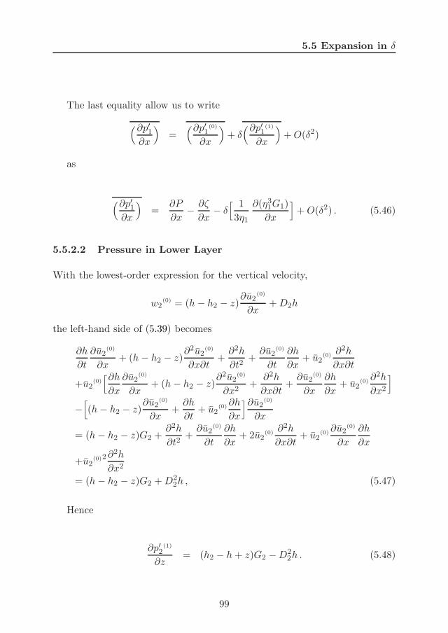
5.5 Expansion in δ
The last equality allow us to write
(∂p′1∂x
)=
(∂p′1(0)
∂x
)+ δ(∂p′1
(1)
∂x
)+ O(δ2)
as
(∂p′1∂x
)=
∂P
∂x− ∂ζ
∂x− δ[ 1
3η1
∂(η31G1)
∂x
]+ O(δ2) . (5.46)
5.5.2.2 Pressure in Lower Layer
With the lowest-order expression for the vertical velocity,
w2(0) = (h − h2 − z)
∂u2(0)
∂x+ D2h
the left-hand side of (5.39) becomes
∂h
∂t
∂u2(0)
∂x+ (h − h2 − z)
∂2u2(0)
∂x∂t+
∂2h
∂t2+
∂u2(0)
∂t
∂h
∂x+ u2
(0) ∂2h
∂x∂t
+u2(0)
[∂h
∂x
∂u2(0)
∂x+ (h − h2 − z)
∂2u2(0)
∂x2+
∂2h
∂x∂t+
∂u2(0)
∂x
∂h
∂x+ u2
(0) ∂2h
∂x2
]
−[(h − h2 − z)
∂u2(0)
∂x+
∂h
∂t+ u2
(0) ∂h
∂x
]∂u2(0)
∂x
= (h − h2 − z)G2 +∂2h
∂t2+
∂u2(0)
∂t
∂h
∂x+ 2u2
(0) ∂2h
∂x∂t+ u2
(0) ∂u2(0)
∂x
∂h
∂x
+u2(0)2 ∂2h
∂x2
= (h − h2 − z)G2 + D22h , (5.47)
Hence
∂p′2(1)
∂z= (h2 − h + z)G2 − D2
2h . (5.48)
99
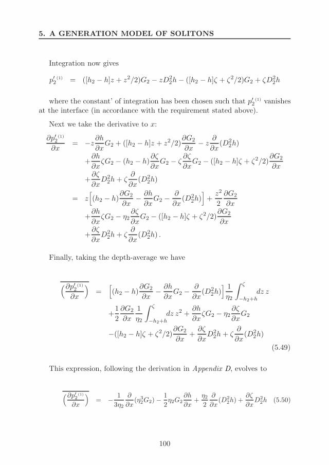
5. A GENERATION MODEL OF SOLITONS
Integration now gives
p′2(1) = ([h2 − h]z + z2/2)G2 − zD2
2h − ([h2 − h]ζ + ζ2/2)G2 + ζD22h
where the constant’ of integration has been chosen such that p′2(1) vanishes
at the interface (in accordance with the requirement stated above).
Next we take the derivative to x:
∂p′2(1)
∂x= −z
∂h
∂xG2 + ([h2 − h]z + z2/2)
∂G2
∂x− z
∂
∂x(D2
2h)
+∂h
∂xζG2 − (h2 − h)
∂ζ
∂xG2 − ζ
∂ζ
∂xG2 − ([h2 − h]ζ + ζ2/2)
∂G2
∂x
+∂ζ
∂xD2
2h + ζ∂
∂x(D2
2h)
= z[(h2 − h)
∂G2
∂x− ∂h
∂xG2 −
∂
∂x(D2
2h)]
+z2
2
∂G2
∂x
+∂h
∂xζG2 − η2
∂ζ
∂xG2 − ([h2 − h]ζ + ζ2/2)
∂G2
∂x
+∂ζ
∂xD2
2h + ζ∂
∂x(D2
2h) .
Finally, taking the depth-average we have
(∂p′2(1)
∂x
)=
[(h2 − h)
∂G2
∂x− ∂h
∂xG2 −
∂
∂x(D2
2h)] 1
η2
∫ ζ
−h2+hdz z
+1
2
∂G2
∂x
1
η2
∫ ζ
−h2+hdz z2 +
∂h
∂xζG2 − η2
∂ζ
∂xG2
−([h2 − h]ζ + ζ2/2)∂G2
∂x+
∂ζ
∂xD2
2h + ζ∂
∂x(D2
2h)
(5.49)
This expression, following the derivation in Appendix D, evolves to
(∂p′2(1)
∂x
)= − 1
3η2
∂
∂x(η3
2G2) −1
2η2G2
∂h
∂x+
η2
2
∂
∂x(D2
2h) +∂ζ
∂xD2
2h (5.50)
100
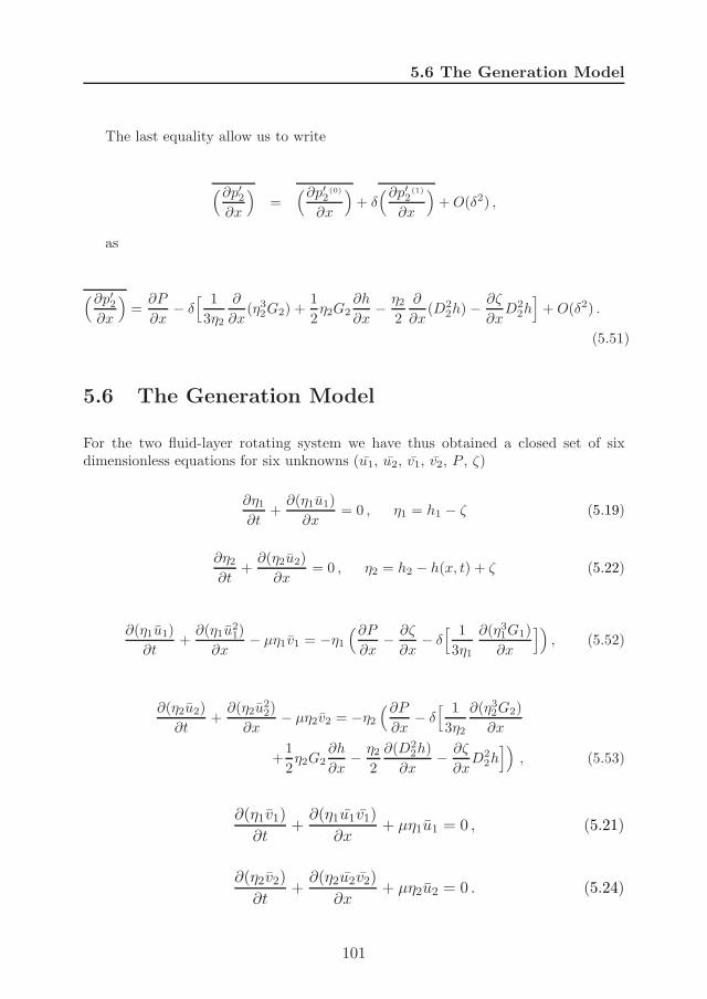
5.6 The Generation Model
The last equality allow us to write
(∂p′2∂x
)=
(∂p′2(0)
∂x
)+ δ(∂p′2
(1)
∂x
)+ O(δ2) ,
as
(∂p′2∂x
)=
∂P
∂x− δ[ 1
3η2
∂
∂x(η3
2G2) +1
2η2G2
∂h
∂x− η2
2
∂
∂x(D2
2h) − ∂ζ
∂xD2
2h]
+ O(δ2) .
(5.51)
5.6 The Generation Model
For the two fluid-layer rotating system we have thus obtained a closed set of sixdimensionless equations for six unknowns (u1, u2, v1, v2, P , ζ)
∂η1
∂t+
∂(η1u1)
∂x= 0 , η1 = h1 − ζ (5.19)
∂η2
∂t+
∂(η2u2)
∂x= 0 , η2 = h2 − h(x, t) + ζ (5.22)
∂(η1u1)
∂t+
∂(η1u21)
∂x− µη1v1 = −η1
(∂P
∂x− ∂ζ
∂x− δ[ 1
3η1
∂(η31G1)
∂x
]), (5.52)
∂(η2u2)
∂t+
∂(η2u22)
∂x− µη2v2 = −η2
(∂P
∂x− δ[ 1
3η2
∂(η32G2)
∂x
+1
2η2G2
∂h
∂x− η2
2
∂(D22h)
∂x− ∂ζ
∂xD2
2h])
, (5.53)
∂(η1v1)
∂t+
∂(η1u1v1)
∂x+ µη1u1 = 0 , (5.21)
∂(η2v2)
∂t+
∂(η2u2v2)
∂x+ µη2u2 = 0 . (5.24)
101
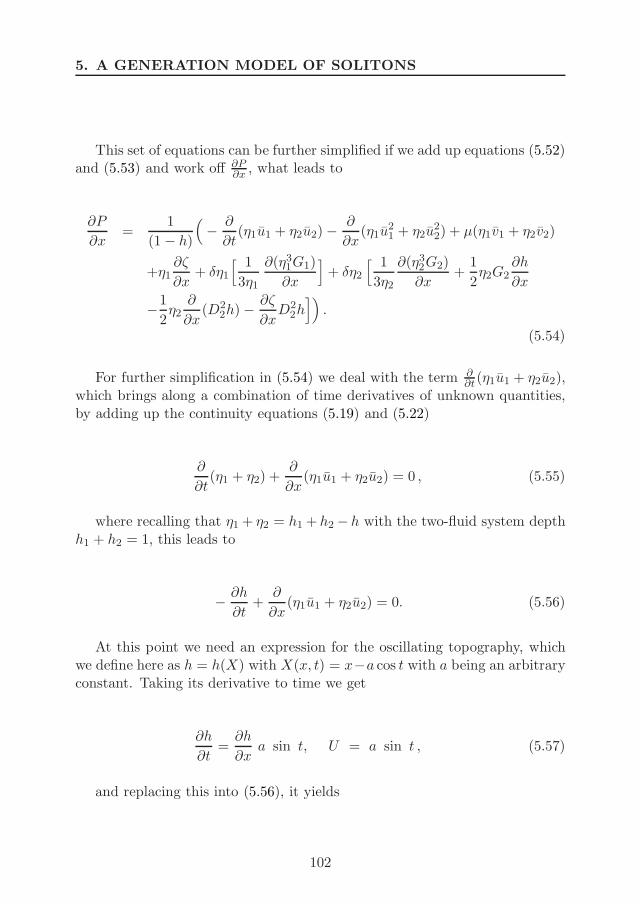
5. A GENERATION MODEL OF SOLITONS
This set of equations can be further simplified if we add up equations (5.52)and (5.53) and work off ∂P
∂x , what leads to
∂P
∂x=
1
(1 − h)
(− ∂
∂t(η1u1 + η2u2) −
∂
∂x(η1u
21 + η2u
22) + µ(η1v1 + η2v2)
+η1∂ζ
∂x+ δη1
[ 1
3η1
∂(η31G1)
∂x
]+ δη2
[ 1
3η2
∂(η32G2)
∂x+
1
2η2G2
∂h
∂x
−1
2η2
∂
∂x(D2
2h) − ∂ζ
∂xD2
2h])
.
(5.54)
For further simplification in (5.54) we deal with the term ∂∂t(η1u1 + η2u2),
which brings along a combination of time derivatives of unknown quantities,by adding up the continuity equations (5.19) and (5.22)
∂
∂t(η1 + η2) +
∂
∂x(η1u1 + η2u2) = 0 , (5.55)
where recalling that η1 + η2 = h1 + h2 − h with the two-fluid system depthh1 + h2 = 1, this leads to
− ∂h
∂t+
∂
∂x(η1u1 + η2u2) = 0. (5.56)
At this point we need an expression for the oscillating topography, whichwe define here as h = h(X) with X(x, t) = x−a cos t with a being an arbitraryconstant. Taking its derivative to time we get
∂h
∂t=
∂h
∂xa sin t, U = a sin t , (5.57)
and replacing this into (5.56), it yields
102
5.6 The Generation Model
∂
∂x(η1u1 + η2u2) = U
∂h
∂x, (5.58)
The latter expression can be now integrated in x following
η1u1 + η2u2 = Uh + A(t) , (5.59)
where we assume that initially u1 = u2 = U = 0 so that A(t) = 0
η1u1 + η2u2 = Uh , (5.60)
and, consequently,
∂
∂t(η1u1 + η2u2) =
∂
∂t(Uh) , (5.61)
which, finally, allow us to replace the term ∂∂t(η1u1+η2u2) (unknown quan-
tity) by ∂∂t(Uh) (known quantity) into (5.54) for simplification of ∂P
∂x
∂P
∂x=
1
(1 − h)
(− ∂
∂t(Uh) − ∂
∂x(η1u
21 + η2u
22) + µ(η1v1 + η2v2) + η1
∂ζ
∂x
+δη1
[ 1
3η1
∂(η31G1)
∂x
]+ δη2
[ 1
3η2
∂(η32G2)
∂x+
η2G2
2
∂h
∂x− η2
2
∂(D22h)
∂x
−∂ζ
∂xD2
2h])
. (5.62)
For further reduction of the horizontal momentum equation for u1 (5.52),we introduce here simplifications made in (5.34), what results in
∂u1
∂t+ u1
∂u1
∂x− µv1 = −∂P
∂x+
∂ζ
∂x+ δ[η1
∂η1
∂xG1 +
η21
3
∂G1
∂x
]+ O(δ2) (5.63)
103
5. A GENERATION MODEL OF SOLITONS
where we replace ∂P∂x by its equivalent expression above, what yields
∂u1
∂t+ u1
∂u1
∂x+ µv1 =
∂ζ
∂x+
1
(1 − h)
(∂(Uh)
∂t+
∂
∂x(η1u
21 + η2u
22)
−µ(η1v1 + η2v2) − η1∂ζ
∂x
)+ δ(1 − η1
(1 − h)
)[η1G1
∂η1
∂x+
η21
3
∂G1
∂x
]
+δη2
(1 − h)
[− η2G2
∂ζ
∂x− η2
2
3
∂G2
∂x+
η2G2
2
∂h
∂x+
η2
2
∂(D22h)
∂x+
∂ζ
∂xD2
2h]
+ O(δ2).
(5.64)
Finally, our two fluid-layer rotating system has been simplified throughoutthis section from a set of six dimensionless equations for six unknowns (u1,u2, v1, v2, P , ζ) to a set of five dimensionless equations for five unknowns (u1,u2, v1, v2, ζ). It is important to recall that, on the way of working off ∂P
∂x ,we obtained the expression (5.60), which is a much simpler equation for u2
than (5.53). To conclude with the work of simplifying our set of equations, be-low we introduce simplifications made in (5.35) for the horizontal momentumequations of vi (5.37) and present our generation model of solitons as
∂u1
∂t+ u1
∂u1
∂x+ µv1 =
∂ζ
∂x+
1
(1 − h)
(∂(Uh)
∂t+
∂
∂x(η1u
21 + η2u
22)
−µ(η1v1 + η2v2) − η1∂ζ
∂x
)+ δ(1 − η1
(1 − h)
)[η1G1
∂η1
∂x+
η21
3
∂G1
∂x
]
+δη2
(1 − h)
[− η2G2
∂ζ
∂x− η2
2
3
∂G2
∂x+
η2G2
2
∂h
∂x+
η2
2
∂(D22h)
∂x+
∂ζ
∂xD2
2h]
+ O(δ2)
(5.64)
u2 =Uh − η1u1
η2, (5.60)
∂v1
∂t+ u1
∂v1
∂x+ µu1 = 0 + O(δ2) , (5.65)
∂v2
∂t+ µu2 + u2
∂v2
∂x= 0 + O(δ2) , (5.66)
104
5.7 Numerical Modeling
∂ζ
∂t− (h1 − ζ)
∂u1
∂x+ u1
∂ζ
∂x= 0 . (5.38)
5.7 Numerical Modeling
We solve the fully nonlinear generation model using numerical techniques, i.e.equations will be discretized and solved following a time stepping algorithmfor a certain space-time grid. Throughout this section we detail how theset of equations which composes the model (5.64, 5.60, 5.37, 5.38) is solvednumerically.
5.7.1 Numerical Strategy
Firstly we define a grid in time and space for discretization of the variousderivatives of the system. Then,
tn = n∆t and xj = j∆x
are introduced for integer values of n (time-step) and j (spatial-step), where∆t and ∆x are the magnitude of the steps. Hence, we can easily describe timeand spatial dependent variables, e.g. y(tn, xj), at any time and position. Thus,yn
j means the value of the variable y at the current time and spatial-step, nand j, respectively. And, consequently, n + 1 would represent the ‘next time-step’, and so n − 1 the ‘previous time-step’, what applies analogously for j inthe space grid. This notation help us to determine grid points and distinguishbetween known and unknown values at every time step, what is important todesign an efficient numerical strategy to solve our equations.
We discretize the various derivatives in the model with centered differenceapproximations (Durran, 1999) as follows
∂y
∂t(tn, xj) =
yn+1j − yn
j
∆t, (5.67)
105
5. A GENERATION MODEL OF SOLITONS
∂y
∂x(tn, xj) =
ynj+1 − yn
j
∆t, (5.68)
∂2y
∂x2(tn, xj) =
ynj+1 − 2yn
j + ynj−1
(∆x)2, (5.69)
∂2y
∂x∂t(tn, xj) =
yn+1j+1 − yn
j+1 − (yn+1j−1 − yn
j−1)
2∆x∆t, (5.70)
∂3y
∂x2∂t(tn, xj) =s
yn+1j+1 − yn
j+1 − 2(yn+1j − yn
j ) + (yn+1j−1 − yn
j−1)
(∆x)2∆t. (5.71)
Initiatilly the system is at rest with mean horizontal velocities, ui and vi,and displacement of the interface, ζ, being all zero at the first two time levels(n− 1, n), what represent the initialization fields. The thickness of the upper,h1, and lower layer, h2, together with the topography, h(X), draw the scenariowhere the two-layer system runs.
At the next time-step (n+1), we start to move the topography to the rightcreating the effect of a tidal motion flowing to the left. For given U (velocity ofmoving topography, (5.57)) and time-step, the excursion of the topography isa known quantity which is used to shift (first, second and third) spatial deriva-tives of h(X) at every new time-step. The momentum (5.37) and continuity(5.38) equations can now be solved for v1
n+1j , v2
n+1j and ζn+1
j at all j posi-tions in terms of the known quantities at the previous two time levels (n−1, n).
The goal consists on getting all terms with time-derivatives in the left-handside of every equation which composes our model, leaving remaining terms inthe right-hand side. At the last stage, we look for an expression in the form
∂y
∂t= Y (tn, xj) (5.72)
106

5.7 Numerical Modeling
where Y (tn, xj) represents a collection of known variables whose values maybe dependent on time and/or space. If we now discretize the derivative in theexpression above, we get
yn+1j − yn
j
∆t= Y (tn, xj) (5.73)
where yn+1j is an unknown quantity which can be expressed for all j posi-
tions in terms of the known quantities of the previous time-levels of y(tn, xj)and Y (tn, xj). This operation is solved numerically using third-order Adams-Bashforth approximation (Durran, 1999) as
yn+1j = yn
j +∆t
12
(23Y n
j − 16Y n−1j + 5Y n−2
j
)(5.74)
This is the idea we keep in mind, we calculate values at the new time-stepsby using known values at the previous time-steps for all spatial positions.Hence, we need an scheme which coherently solve our equations in a way thatwe always count with the required known values to move our system to thenew time-step over the space domain.
To this end, equations for v1 (5.65), v2 (5.66) and ζ (5.38) are easily reor-ganized to be solved numerically with the time derivative in the left hand-sidefollowing
∂v1
∂t= −u1
∂v1
∂x− µu1 + O(δ2) (5.65)
∂v2
∂t= −µu2 − u2
∂v2
∂x+ O(δ2) (5.66)
∂ζ
∂t= (h1 − ζ)
∂u1
∂x− u1
∂ζ
∂x(5.38)
as required for applying Adams-Bashforth appromixation.
107
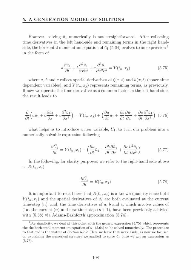
5. A GENERATION MODEL OF SOLITONS
However, solving u1 numerically is not straightforward. After collectingtime derivatives in the left hand-side and remaining terms in the right hand-side, the horizontal momemtum equation of u1 (5.64) evolves to an expression 1
in the form of
a∂u1
∂t+ b
∂2u1
∂x∂t+ c
∂3u1
∂x2∂t= Y (tn, xj) (5.75)
where a, b and c collect spatial derivatives of ζ(x, t) and h(x, t) (space-timedependent variables); and Y (tn, xj) represents remaining terms, as previously.If now we operate the time derivative as a common factor in the left-hand side,the result leads to
∂
∂t
(au1 + b
∂u1
∂x+ c
∂2u1
∂x2
)= Y (tn, xj) +
(∂a
∂tu1 +
∂b
∂t
∂u1
∂x+
∂c
∂t
∂2u1
∂x2
)(5.76)
what helps us to introduce a new variable, U1, to turn our problem into anumerically solvable expression following
∂U1
∂t= Y (tn, xj) +
(∂a
∂tu1 +
∂b
∂t
∂u1
∂x+
∂c
∂t
∂2u1
∂x2
)(5.77)
In the following, for clarity purposes, we refer to the right-hand side aboveas R(tn, xj)
∂U1
∂t= R(tn, xj) (5.78)
It is important to recall here that R(tn, xj) is a known quantity since bothY (tn, xj) and the spatial derivatives of u1 are both evaluated at the currenttime-step (n); and, the time derivatives of a, b and c, which involve values ofζ at the current (n) and new time-step (n + 1), have been previously achiviedwith (5.38) via Adams-Bashforth approximation (5.74).
1For simplicity, we deal at this point with the generic expression (5.75) which representsthe the horizontal momemtum equation of u1 (5.64) to be solved numerically. The procedureto that end is the matter of Section 5.7.2. Here we leave that work aside, as now we focusedon explaining the numerical strategy we applied to solve u1 once we get an expression as(5.75).
108
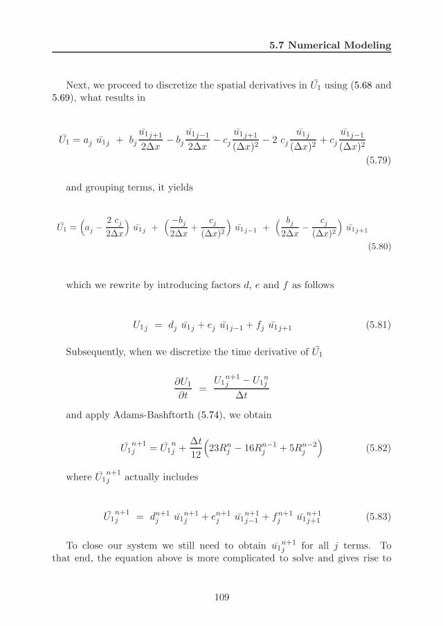
5.7 Numerical Modeling
Next, we proceed to discretize the spatial derivatives in U1 using (5.68 and5.69), what results in
U1 = aj u1j + bj
u1j+1
2∆x− bj
u1j−1
2∆x− cj
u1j+1
(∆x)2− 2 cj
u1j
(∆x)2+ cj
u1j−1
(∆x)2
(5.79)
and grouping terms, it yields
U1 =(aj −
2 cj
2∆x
)u1j +
( −bj
2∆x+
cj
(∆x)2
)u1j−1 +
( bj
2∆x−
cj
(∆x)2
)u1j+1
(5.80)
which we rewrite by introducing factors d, e and f as follows
U1j = dj u1j + ej u1j−1 + fj u1j+1 (5.81)
Subsequently, when we discretize the time derivative of U1
∂U1
∂t=
U1n+1j − U1
nj
∆t
and apply Adams-Bashftorth (5.74), we obtain
U1n+1j = U1
nj +
∆t
12
(23Rn
j − 16Rn−1j + 5Rn−2
j
)(5.82)
where U1n+1j actually includes
U1n+1j = dn+1
j u1n+1j + en+1
j u1n+1j−1 + fn+1
j u1n+1j+1 (5.83)
To close our system we still need to obtain u1n+1j for all j terms. To
that end, the equation above is more complicated to solve and gives rise to
109
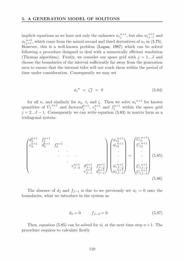
5. A GENERATION MODEL OF SOLITONS
implicit equations as we have not only the unknown u1n+1j , but also u1
n+1j−1 and
u1n+1j+1 , which come from the mixed second and third derivatives of u1 in (5.75).
However, this is a well-known problem (Logan, 1987) which can be solvedfollowing a procedure designed to deal with a numerically efficient resolution(Thomas algorithm). Firstly, we consider our space grid with j = 1...J andchoose the boundaries of the interval sufficiently far away from the generationarea to ensure that the internal tides will not reach them within the period oftime under consideration. Consequently we may set
u1n = ζn
J = 0 (5.84)
for all n, and similarly for u2, vi and ζ. Then we solve u1n+1 for known
quantities of U1n+1
and factorsdn+1j , en+1
j and fn+1j within the space grid
j = 2...J − 1. Consequently we can write equation (5.83) in matrix form as atridiagonal system:
dn+12 fn+1
2
en+13 dn+1
3 fn+13
. . .. . .
. . .
en+1J−2 dn+1
J−2 fn+1J−2
en+1J−1 dn+1
J−1
u1n+12
u1n+13
.
.
.
u1n+1J−2
u1n+1J−1
=
U1n+11
U1n+12
.
.
.
U1n+1J−2
U1n+1J−1
(5.85)
(5.86)
The absence of d2 and fJ−1 is due to we previously set u1 = 0 onto theboundaries, what we introduce in the system as
d2 = 0 fJ−2 = 0 (5.87)
Then, equation (5.85) can be solved for u1 at the next time step n+1. Theprocedure requires to calculate firstly
110
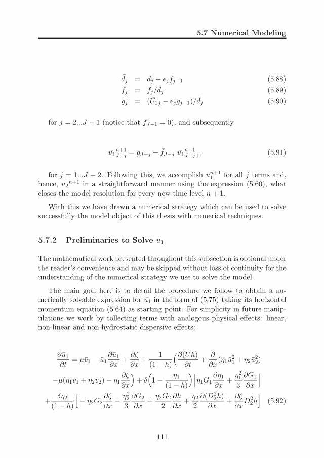
5.7 Numerical Modeling
dj = dj − ejfj−1 (5.88)
fj = fj/dj (5.89)
gj = (U1j − ejgj−1)/dj (5.90)
for j = 2...J − 1 (notice that fJ−1 = 0), and subsequently
u1n+1J−j = gJ−j − fJ−j u1
n+1J−j+1 (5.91)
for j = 1...J − 2. Following this, we accomplish un+11 for all j terms and,
hence, u2n+1 in a straightforward manner using the expression (5.60), what
closes the model resolution for every new time level n + 1.
With this we have drawn a numerical strategy which can be used to solvesuccessfully the model object of this thesis with numerical techniques.
5.7.2 Preliminaries to Solve u1
The mathematical work presented throughout this subsection is optional underthe reader’s convenience and may be skipped without loss of continuity for theunderstanding of the numerical strategy we use to solve the model.
The main goal here is to detail the procedure we follow to obtain a nu-merically solvable expression for u1 in the form of (5.75) taking its horizontalmomentum equation (5.64) as starting point. For simplicity in future manip-ulations we work by collecting terms with analogous physical effects: linear,non-linear and non-hydrostatic dispersive effects:
∂u1
∂t= µv1 − u1
∂u1
∂x+
∂ζ
∂x+
1
(1 − h)
(∂(Uh)
∂t+
∂
∂x(η1u
21 + η2u
22)
−µ(η1v1 + η2v2) − η1∂ζ
∂x
)+ δ(1 − η1
(1 − h)
)[η1G1
∂η1
∂x+
η21
3
∂G1
∂x
]
+δη2
(1 − h)
[− η2G2
∂ζ
∂x− η2
2
3
∂G2
∂x+
η2G2
2
∂h
∂x+
η2
2
∂(D22h)
∂x+
∂ζ
∂xD2
2h]
(5.92)
111
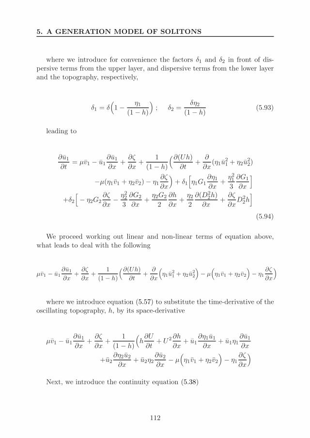
5. A GENERATION MODEL OF SOLITONS
where we introduce for convenience the factors δ1 and δ2 in front of dis-persive terms from the upper layer, and dispersive terms from the lower layerand the topography, respectively,
δ1 = δ(1 − η1
(1 − h)
); δ2 =
δη2
(1 − h)(5.93)
leading to
∂u1
∂t= µv1 − u1
∂u1
∂x+
∂ζ
∂x+
1
(1 − h)
(∂(Uh)
∂t+
∂
∂x(η1u
21 + η2u
22)
−µ(η1v1 + η2v2) − η1∂ζ
∂x
)+ δ1
[η1G1
∂η1
∂x+
η21
3
∂G1
∂x
]
+δ2
[− η2G2
∂ζ
∂x− η2
2
3
∂G2
∂x+
η2G2
2
∂h
∂x+
η2
2
∂(D22h)
∂x+
∂ζ
∂xD2
2h]
(5.94)
We proceed working out linear and non-linear terms of equation above,what leads to deal with the following
µv1 − u1
∂u1
∂x+
∂ζ
∂x+
1
(1 − h)
(∂(Uh)
∂t+
∂
∂x
(η1u
21 + η2u
22
)− µ
(η1v1 + η2v2
)− η1
∂ζ
∂x
)
where we introduce equation (5.57) to substitute the time-derivative of theoscillating topography, h, by its space-derivative
µv1 − u1∂u1
∂x+
∂ζ
∂x+
1
(1 − h)
(h
∂U
∂t+ U2 ∂h
∂x+ u1
∂η1u1
∂x+ u1η1
∂u1
∂x
+u2∂η2u2
∂x+ u2η2
∂u2
∂x− µ
(η1v1 + η2v2
)− η1
∂ζ
∂x
)
Next, we introduce the continuity equation (5.38)
112
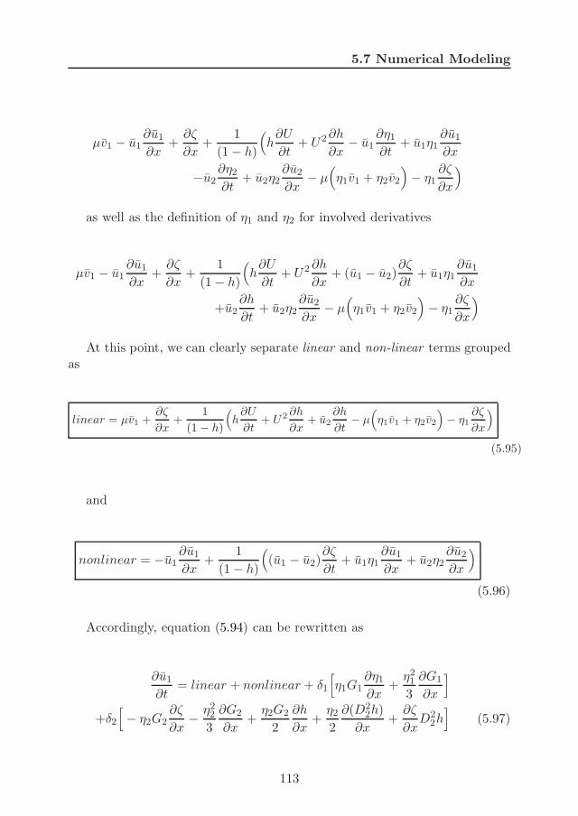
5.7 Numerical Modeling
µv1 − u1∂u1
∂x+
∂ζ
∂x+
1
(1 − h)
(h
∂U
∂t+ U2 ∂h
∂x− u1
∂η1
∂t+ u1η1
∂u1
∂x
−u2∂η2
∂t+ u2η2
∂u2
∂x− µ
(η1v1 + η2v2
)− η1
∂ζ
∂x
)
as well as the definition of η1 and η2 for involved derivatives
µv1 − u1∂u1
∂x+
∂ζ
∂x+
1
(1 − h)
(h
∂U
∂t+ U2 ∂h
∂x+ (u1 − u2)
∂ζ
∂t+ u1η1
∂u1
∂x
+u2∂h
∂t+ u2η2
∂u2
∂x− µ
(η1v1 + η2v2
)− η1
∂ζ
∂x
)
At this point, we can clearly separate linear and non-linear terms groupedas
linear = µv1 +∂ζ
∂x+
1
(1 − h)
(h
∂U
∂t+ U2 ∂h
∂x+ u2
∂h
∂t− µ
(η1v1 + η2v2
)− η1
∂ζ
∂x
)
(5.95)
and
nonlinear = −u1∂u1
∂x+
1
(1 − h)
((u1 − u2)
∂ζ
∂t+ u1η1
∂u1
∂x+ u2η2
∂u2
∂x
)
(5.96)
Accordingly, equation (5.94) can be rewritten as
∂u1
∂t= linear + nonlinear + δ1
[η1G1
∂η1
∂x+
η21
3
∂G1
∂x
]
+δ2
[− η2G2
∂ζ
∂x− η2
2
3
∂G2
∂x+
η2G2
2
∂h
∂x+
η2
2
∂(D22h)
∂x+
∂ζ
∂xD2
2h]
(5.97)
113
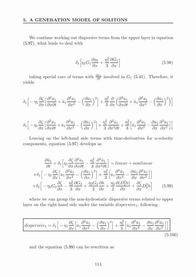
5. A GENERATION MODEL OF SOLITONS
We continue working out dispersive terms from the upper layer in equation(5.97), what leads to deal with
δ1
[η1G1
∂η1
∂x+
η21
3
∂G1
∂x
](5.98)
taking special care of terms with ∂u1∂t involved in G1 (5.41). Therefore, it
yields
δ1
[− η1
∂ζ
∂x
[∂2u1
∂x∂t+ u1
∂2u1
∂x2−(∂u1
∂x
)2]+
η21
3
∂
∂x
(∂2u1
∂x∂t+ u1
∂2u1
∂x2−(∂u1
∂x
)2)]
δ1
[−η1
∂ζ
∂x
[∂2u1
∂x∂t+ u1
∂2u1
∂x2−(∂u1
∂x
)2]+
η21
3
∂3u1
∂x2∂t+
η21
3
[u1
∂3u1
∂x3− ∂u1
∂x
∂2u1
∂x2
]]
Leaving on the left-hand side terms with time-derivatives for u-velocitycomponents, equation (5.97) develops as
∂u1
∂t+ δ1
[η1
∂ζ
∂x
∂2u1
∂x∂t− η2
1
3
∂3u1
∂x2∂t
]= linear + nonlinear
+δ1
[− η1
∂ζ
∂x
[u1
∂2u1
∂x2−(∂u1
∂x
)2]+
η21
3
[u1
∂3u1
∂x3− ∂u1
∂x
∂2u1
∂x2
]]
+δ2
[− η2G2
∂ζ
∂x− η2
2
3
∂G2
∂x+
η2G2
2
∂h
∂x+
η2
2
∂(D22h)
∂x+
∂ζ
∂xD2
2h]
(5.99)
where we can group the non-hydrostatic dispersive terms related to upperlayer on the right-hand side under the variable dispersive1, following
dispersive1 = δ1
[− η1
∂ζ
∂x
[u1
∂2u1
∂x2−(∂u1
∂x
)2]+
η21
3
[u1
∂3u1
∂x3− ∂u1
∂x
∂2u1
∂x2
]]
(5.100)
and the equation (5.99) can be rewritten as
114
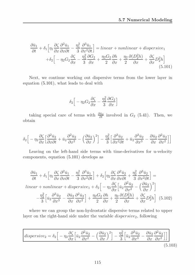
5.7 Numerical Modeling
∂u1
∂t+ δ1
[η1
∂ζ
∂x
∂2u1
∂x∂t− η2
1
3
∂3u1
∂x2∂t
]= linear + nonlinear + dispersive1
+δ2
[− η2G2
∂ζ
∂x− η2
2
3
∂G2
∂x+
η2G2
2
∂h
∂x+
η2
2
∂(D22h)
∂x+
∂ζ
∂xD2
2h]
(5.101)
Next, we continue working out dispersive terms from the lower layer inequation (5.101), what leads to deal with
δ2
[− η2G2
∂ζ
∂x− η2
2
3
∂G2
∂x
]
taking special care of terms with ∂u2∂t involved in G2 (5.41). Then, we
obtain
δ2
[− η2
∂ζ
∂x
[∂2u2
∂x∂t+ u2
∂2u2
∂x2−(∂u2
∂x
)2]− η2
2
3
[ ∂3u2
∂x2∂t+ u2
∂3u2
∂x3− ∂u2
∂x
∂2u2
∂x2
]]
Leaving on the left-hand side terms with time-derivatives for u-velocitycomponents, equation (5.101) develops as
∂u1
∂t+ δ1
[η1
∂ζ
∂x
∂2u1
∂x∂t− η2
1
3
∂3u1
∂x2∂t
]+ δ2
[η2
∂ζ
∂x
∂2u2
∂x∂t+
η22
3
∂3u2
∂x2∂t
]=
linear + nonlinear + dispersive1 + δ2
[− η2
∂ζ
∂x
[u2
∂2u2
∂x2−(∂u2
∂x
)2]
−η22
3
[u2
∂3u2
∂x3− ∂u2
∂x
∂2u2
∂x2
]+
η2G2
2
∂h
∂x+
η2
2
∂(D22h)
∂x+
∂ζ
∂xD2
2h]
(5.102)
where we can group the non-hydrostatic dispersive terms related to upperlayer on the right-hand side under the variable dispersive2, following
dispersive2 = δ2
[− η2
∂ζ
∂x
[u2
∂2u2
∂x2−(∂u2
∂x
)2]− η2
2
3
[u2
∂3u2
∂x3− ∂u2
∂x
∂2u2
∂x2
]]
(5.103)
115

5. A GENERATION MODEL OF SOLITONS
and the equation (5.102) can be rewritten as
∂u1
∂t+ δ1
[η1
∂ζ
∂x
∂2u1
∂x∂t− η2
1
3
∂3u1
∂x2∂t
]+ δ2
[η2
∂ζ
∂x
∂2u2
∂x∂t+
η22
3
∂3u2
∂x2∂t
]=
linear + nonlinear + dispersive1 + dispersive2
+δ2
[η2G2
2
∂h
∂x+
η2
2
∂(D22h)
∂x+
∂ζ
∂xD2
2h]
(5.104)
At this stage it is important to notice that we have obtained in equation(5.104) terms with time derivatives of u2 on the left-hand side. Once wefinish to turn out all dispersive terms from topography, we will deal with thecomplete left-hand side, grouping terms and substituting u2 in terms of u1
following Appendix E.
Now we continue working out dispersive terms from the topography inequation (5.104), what leads to deal with
δ2
[η2G2
2
∂h
∂x+
η2
2
∂(D22h)
∂x+
∂ζ
∂xD2
2h]
taking special care of terms with ∂u2∂t involved in G2 (5.41). Then we get
δ2
[η2
2
∂h
∂x
[∂2u2
∂x∂t+ u2
∂2u2
∂x2−(∂u2
∂x
)2]
+η2
2
∂
∂x
(∂2h
∂t2+
∂u2
∂t
∂h
∂x+ 2u2
∂2h
∂x∂t+ u2
∂u2
∂x
∂h
∂x+ u2
2
∂2h
∂x2
)
+∂ζ
∂x
[∂2h
∂t2+
∂u2
∂t
∂h
∂x+ 2u2
∂2h
∂x∂t+ u2
∂u2
∂x
∂h
∂x+ u2
2
∂2h
∂x2
]](5.105)
where making some simplifications we obtain
δ2
[η2
∂2u2
∂x∂t
∂h
∂x+ η2u2
∂2u2
∂x2
∂h
∂x+
η2
2
[ ∂3h
∂x∂t2+
∂u2
∂t
∂2h
∂x2+ 2
∂u2
∂x
∂2h
∂x∂t
+2u2∂3h
∂x2∂t+ 3u2
∂u2
∂x
∂2h
∂x2+ u2
2
∂3h
∂x3
]+
∂ζ
∂x
[∂2h
∂t2+
∂u2
∂t
∂h
∂x+ 2u2
∂2h
∂x∂t
+u2∂u2
∂x
∂h
∂x+ u2
2
∂2h
∂x2
]]
(5.106)
116
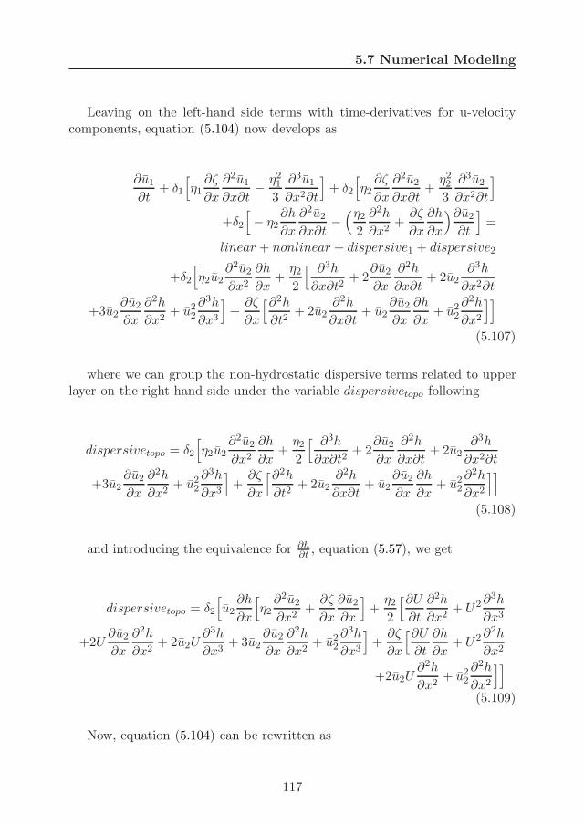
5.7 Numerical Modeling
Leaving on the left-hand side terms with time-derivatives for u-velocitycomponents, equation (5.104) now develops as
∂u1
∂t+ δ1
[η1
∂ζ
∂x
∂2u1
∂x∂t− η2
1
3
∂3u1
∂x2∂t
]+ δ2
[η2
∂ζ
∂x
∂2u2
∂x∂t+
η22
3
∂3u2
∂x2∂t
]
+δ2
[− η2
∂h
∂x
∂2u2
∂x∂t−(η2
2
∂2h
∂x2+
∂ζ
∂x
∂h
∂x
)∂u2
∂t
]=
linear + nonlinear + dispersive1 + dispersive2
+δ2
[η2u2
∂2u2
∂x2
∂h
∂x+
η2
2
[ ∂3h
∂x∂t2+ 2
∂u2
∂x
∂2h
∂x∂t+ 2u2
∂3h
∂x2∂t
+3u2∂u2
∂x
∂2h
∂x2+ u2
2
∂3h
∂x3
]+
∂ζ
∂x
[∂2h
∂t2+ 2u2
∂2h
∂x∂t+ u2
∂u2
∂x
∂h
∂x+ u2
2
∂2h
∂x2
]]
(5.107)
where we can group the non-hydrostatic dispersive terms related to upperlayer on the right-hand side under the variable dispersivetopo following
dispersivetopo = δ2
[η2u2
∂2u2
∂x2
∂h
∂x+
η2
2
[ ∂3h
∂x∂t2+ 2
∂u2
∂x
∂2h
∂x∂t+ 2u2
∂3h
∂x2∂t
+3u2∂u2
∂x
∂2h
∂x2+ u2
2
∂3h
∂x3
]+
∂ζ
∂x
[∂2h
∂t2+ 2u2
∂2h
∂x∂t+ u2
∂u2
∂x
∂h
∂x+ u2
2
∂2h
∂x2
]]
(5.108)
and introducing the equivalence for ∂h∂t , equation (5.57), we get
dispersivetopo = δ2
[u2
∂h
∂x
[η2
∂2u2
∂x2+
∂ζ
∂x
∂u2
∂x
]+
η2
2
[∂U
∂t
∂2h
∂x2+ U2 ∂3h
∂x3
+2U∂u2
∂x
∂2h
∂x2+ 2u2U
∂3h
∂x3+ 3u2
∂u2
∂x
∂2h
∂x2+ u2
2∂3h
∂x3
]+
∂ζ
∂x
[∂U
∂t
∂h
∂x+ U2 ∂2h
∂x2
+2u2U∂2h
∂x2+ u2
2
∂2h
∂x2
]]
(5.109)
Now, equation (5.104) can be rewritten as
117

5. A GENERATION MODEL OF SOLITONS
∂u1
∂t+ δ1
[η1
∂ζ
∂x
∂2u1
∂x∂t− η2
1
3
∂3u1
∂x2∂t
]+ δ2
[η2
∂ζ
∂x
∂2u2
∂x∂t+
η22
3
∂3u2
∂x2∂t
]
+δ2
[− η2
∂h
∂x
∂2u2
∂x∂t−(η2
2
∂2h
∂x2+
∂ζ
∂x
∂h
∂x
)∂u2
∂t
]=
linear + nonlinear + dispersive1 + dispersive2 + dispersivetopo (5.110)
Finally, we are interested in substituting u2 in terms of u1 for time-derivativeson the left-hand side of equation (5.110) with the equivalences described inAppendix E. With this aim, we first proceed to group common terms on theleft-hand side
∂u1
∂t+ δ1
[η1
∂ζ
∂x
∂2u1
∂x∂t− η2
1
3
∂3u1
∂x2∂t
]+ δ2
[(η2
∂ζ
∂x− η2
∂h
∂x
)∂2u2
∂x∂t+
η22
3
∂3u2
∂x2∂t
−(η2
2
∂2h
∂x2+
∂ζ
∂x
∂h
∂x
)∂u2
∂t
]
= linear + nonlinear + dispersive1 + dispersive2 + dispersivetopo
(5.111)
and then substitute u2 in terms of u1 on the basis of Appendix E (wherewe introduce φ)
∂u1
∂t+ δ1
[η1
∂ζ
∂x
∂2u1
∂x∂t− η2
1
3
∂3u1
∂x2∂t
]+ δ2
[(η2
∂ζ
∂x− η2
∂h
∂x
)[− η1
η2
∂2u1
∂x∂t
−∂(η1/η2)
∂x
∂u1
∂t+
∂φ
∂x
]+
η22
3
[− 2
∂(η1/η2)
∂x
∂2u1
∂x∂t− η1
η2
∂3u1
∂x2∂t
−∂2(η1/η2)
∂x2
∂u1
∂t+
∂2φ
∂x2
]−(η2
2
∂2h
∂x2+
∂ζ
∂x
∂h
∂x
)[− η1
η2
∂u1
∂t+ φ
]]=
linear + nonlinear + dispersive1 + dispersive2 + dispersivetopo (5.112)
To finish with this procedure we take terms involving φ to the right-handside and collect terms with same time-derivative of u1 on the left-hand side
118
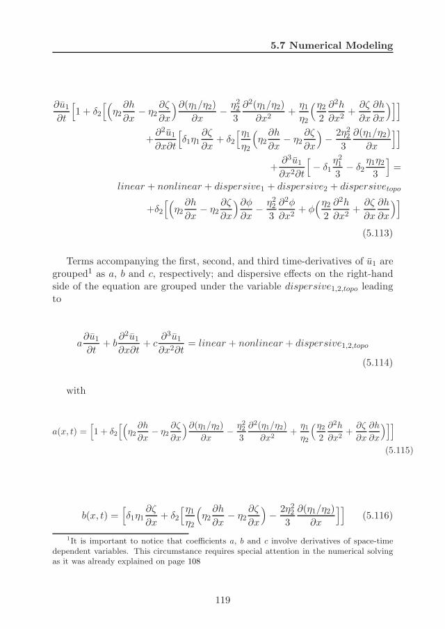
5.7 Numerical Modeling
∂u1
∂t
[1 + δ2
[(η2
∂h
∂x− η2
∂ζ
∂x
)∂(η1/η2)
∂x− η2
2
3
∂2(η1/η2)
∂x2+
η1
η2
(η2
2
∂2h
∂x2+
∂ζ
∂x
∂h
∂x
)]]
+∂2u1
∂x∂t
[δ1η1
∂ζ
∂x+ δ2
[η1
η2
(η2
∂h
∂x− η2
∂ζ
∂x
)− 2η2
2
3
∂(η1/η2)
∂x
]]
+∂3u1
∂x2∂t
[− δ1
η21
3− δ2
η1η2
3
]=
linear + nonlinear + dispersive1 + dispersive2 + dispersivetopo
+δ2
[(η2
∂h
∂x− η2
∂ζ
∂x
)∂φ
∂x− η2
2
3
∂2φ
∂x2+ φ
(η2
2
∂2h
∂x2+
∂ζ
∂x
∂h
∂x
)]
(5.113)
Terms accompanying the first, second, and third time-derivatives of u1 aregrouped1 as a, b and c, respectively; and dispersive effects on the right-handside of the equation are grouped under the variable dispersive1,2,topo leadingto
a∂u1
∂t+ b
∂2u1
∂x∂t+ c
∂3u1
∂x2∂t= linear + nonlinear + dispersive1,2,topo
(5.114)
with
a(x, t) =[1 + δ2
[(η2
∂h
∂x− η2
∂ζ
∂x
)∂(η1/η2)
∂x− η2
2
3
∂2(η1/η2)
∂x2+
η1
η2
(η2
2
∂2h
∂x2+
∂ζ
∂x
∂h
∂x
)]]
(5.115)
b(x, t) =[δ1η1
∂ζ
∂x+ δ2
[η1
η2
(η2
∂h
∂x− η2
∂ζ
∂x
)− 2η2
2
3
∂(η1/η2)
∂x
]](5.116)
1It is important to notice that coefficients a, b and c involve derivatives of space-timedependent variables. This circumstance requires special attention in the numerical solvingas it was already explained on page 108
119
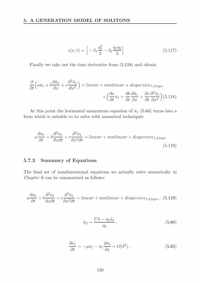
5. A GENERATION MODEL OF SOLITONS
c(x, t) =[− δ1
η21
3− δ2
η1η2
3
](5.117)
Finally we take out the time derivative from (5.118) and obtain
∂
∂t
(au1 + b
∂u1
∂x+ c
∂2u1
∂x2
)= linear + nonlinear + dispersive1,2,topo
+(∂a
∂tu1 +
∂b
∂t
∂u1
∂x+
∂c
∂t
∂2u1
∂x2
)(5.118)
At this point the horizontal momentum equation of u1 (5.64) turns into aform which is suitable to be solve with numerical techniques
a∂u1
∂t+ b
∂2u1
∂x∂t+ c
∂3u1
∂x2∂t= linear + nonlinear + dispersive1,2,topo
(5.119)
5.7.3 Summary of Equations
The final set of nondimensional equations we actually solve numerically inChapter 6 can be summarized as follows:
a∂u1
∂t+ b
∂2u1
∂x∂t+ c
∂3u1
∂x2∂t= linear + nonlinear + dispersive1,2,topo , (5.119)
u2 =Uh − η1u1
η2, (5.60)
∂v1
∂t= −µu1 − u1
∂v1
∂x+ O(δ2) , (5.65)
120
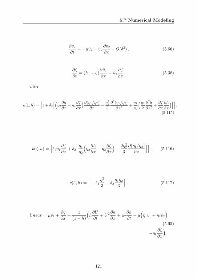
5.7 Numerical Modeling
∂v2
∂t= −µu2 − u2
∂v2
∂x+ O(δ2) , (5.66)
∂ζ
∂t= (h1 − ζ)
∂u1
∂x− u1
∂ζ
∂x. (5.38)
with
a(ζ, h) =[1 + δ2
[(η2
∂h
∂x− η2
∂ζ
∂x
)∂(η1/η2)
∂x− η2
2
3
∂2(η1/η2)
∂x2+
η1
η2
(η2
2
∂2h
∂x2+
∂ζ
∂x
∂h
∂x
)]],
(5.115)
b(ζ, h) =[δ1η1
∂ζ
∂x+ δ2
[η1
η2
(η2
∂h
∂x− η2
∂ζ
∂x
)− 2η2
2
3
∂(η1/η2)
∂x
]], (5.116)
c(ζ, h) =[− δ1
η21
3− δ2
η1η2
3
], (5.117)
linear = µv1 +∂ζ
∂x+
1
(1 − h)
(h
∂U
∂t+ U2 ∂h
∂x+ u2
∂h
∂t− µ
(η1v1 + η2v2
)
(5.95)
−η1∂ζ
∂x
),
121

5. A GENERATION MODEL OF SOLITONS
nonlinear = −u1∂u1
∂x+
1
(1 − h)
((u1 − u2)
∂ζ
∂t+ u1η1
∂u1
∂x+ u2η2
∂u2
∂x
),
(5.96)
dispersive1 = δ1
[− η1
∂ζ
∂x
[u1
∂2u1
∂x2−(∂u1
∂x
)2]+
η21
3
[u1
∂3u1
∂x3− ∂u1
∂x
∂2u1
∂x2
]],
(5.100)
dispersive2 = δ2
[− η2
∂ζ
∂x
[u2
∂2u2
∂x2−(∂u2
∂x
)2]− η2
2
3
[u2
∂3u2
∂x3− ∂u2
∂x
∂2u2
∂x2
]],
(5.103)
dispersivetopo = δ2
[u2
∂h
∂x
[η2
∂2u2
∂x2+
∂ζ
∂x
∂u2
∂x
]+
η2
2
[∂U
∂t
∂2h
∂x2+ U2 ∂3h
∂x3
(5.109)
+2U∂u2
∂x
∂2h
∂x2+ 2u2U
∂3h
∂x3+ 3u2
∂u2
∂x
∂2h
∂x2+ u2
2
∂3h
∂x3
]+
∂ζ
∂x
[∂U
∂t
∂h
∂x+ U2 ∂2h
∂x2
+2u2U∂2h
∂x2+ u2
2
∂2h
∂x2
]],
122
Chapter 6
Numerical Experiments onSolitons1
6.1 Outline
The main goal of this chapter is to present various numerical experimentswhich demonstrate the capability of the model we have derived on reproduc-ing two of the more distinguishable properties attributed to a fully nonlinearset of equations: the generation of ‘table-top’ solitons when approaching thetheoretical maximum amplitude given appropriate initial conditions; and, 2)the appearance of nonlinearitiess under a configuration in which the two-fluidsystem consists of two layers of equal thickness.
In Section6.2 we deal with key aspects about the configuration of the nu-merical experiments before starting the presentation of the main results. InSubsection 6.2.1 we recall to the reader the main components of the two-fuid layer system which configure the model. Discussion on the criteria tochoose the resolution of the space-time grid needed for solving numericallythe modeld is addressed in Subsection 6.2.2. As we have already described,the ‘tide-topography’ interaction is introduced in the model through a movingtopography and a fluid initally at rest; unlike the original problem in which
1Aguiar-Gonzalez B., Gerkema T. A Model for the Generation of Strongly Nonlinear,Weakly Nonhydrostatic Interfacial Waves. In Preparation to be Submitted to an International
refereed Journal
123

6. NUMERICAL EXPERIMENTS ON SOLITONS
a barotropic tidal flow over topography generates internal tides. This situa-tion leads to the question of whether the model can be realistically consideredequivalent to oceanic conditions. Consequently, we use in Subsection 6.2.3 thegeneration model of weakly nonlinear weakly nonhydrostatic solitons derivedin Gerkema (1996), which works with tidal motion, as a benchmark for testingour fully nonlinear weakly nonhydrostatic generation model of solitons, whichworks with moving topography. Next, we summarize in Subsection 6.2.4 themain parameters we set for the numerical experiments shown throughout thechapter.
Firstly we present some simulations on the generation of the linear hydro-static internal tides to test the model in absence of nonlinearities and nonhy-drostatic effects (Section 6.3). Subsequently, we move forward and include thelatter effects in the simulations focusing on two special cases. On one hand, weshow in Section 6.4.1 the generation of strongly nonlinear solitons approach-ing its theoretical limiting amplitude and hence evolving to large-amplitudeflat ‘table-top’ solitons. On the other hand, we deal with two layers of equalthickness and nonlinearities in Section 6.4.2. Conclusions are addressed inSection 6.5.
6.2 Configuration of the Numerical Experiments
6.2.1 The Two-Fluid Layer System
A general diagram of the two-fluid layer system is shown in Figure 6.1. Weassume that the upper and lower layer consists of incompressible, inviscid,homogeneous fluids of density ρ1 and ρ2, and have a thickness of h1 and h2,respectively. The rest level of the interface is located at z = 0, the upwarddirection of the z-axis is positive. Here, ηi represents the thickness of the layer(depending on the interfacial displacement ζ). Furthermore, the upper surfaceis covered by a rigid lid.
The system is supposed to be uniform in the y (i. e. transverse) direction;the topography is consequently assumed to be infinite in that direction. Wemimick the ‘tide-topography’interaction which generates the internal tide inthe system with a moving bottom which oscillates horizontally. However, inorder to facilitate the interpretation of the simulations, we transformed the
124
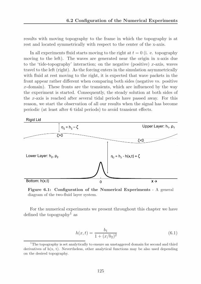
6.2 Configuration of the Numerical Experiments
results with moving topography to the frame in which the topography is atrest and located symmetrically with respect to the center of the x-axis.
In all experiments fluid starts moving to the right at t = 0 (i. e. topographymoving to the left). The waves are generated near the origin in x-axis dueto the ‘tide-topography’ interaction; on the negative (positive) x-axis, wavestravel to the left (right). As the forcing enters in the simulation asymmetricallywith fluid at rest moving to the right, it is expected that wave packets in thefront appear rather different when comparing both sides (negative vs. positivex-domain). These fronts are the transients, which are influenced by the waythe experiment is started. Consequently, the steady solution at both sides ofthe x-axis is reached after several tidal periods have passed away. For thisreason, we start the observation of all our results when the signal has becomeperiodic (at least after 6 tidal periods) to avoid transient effects.
Figure 6.1: Configuration of the Numerical Experiments - A generaldiagram of the two-fluid layer system.
For the numerical experiments we present throughout this chapter we havedefined the topography1 as
h(x, t) =b1
1 + (x/b2)2(6.1)
1The topography is set analytically to ensure an unstaggered domain for second and thirdderivatives of h(x, t). Nevertheless, other analytical functions may be also used dependingon the desired topography.
125
6. NUMERICAL EXPERIMENTS ON SOLITONS
with x being the grid positions in space; and, b1 and b2 being the parameterswhich set the height and width of a symmetric sill, respectively. Also, thetopographic obstacle (ridge, sill, ...) is always centred in the x-axis and thelength of the x-domain is chosen to be large enough to prevent that generatedwaves reach the boundaries.
It is worth while to recall that the oscillation of the topography is includedwithin the model (on page 102) as h = h(X) with X(x, t) = x− a cos t with abeing an arbitrary constant.
6.2.2 Setting the Space-Time Grid
The choice of the steps Λt, Λx introduced in Chapter 5 (Section 5.7) wasbased on two main requirements. Firstly, the resolution in x (Λx) must besufficiently fine to resolve third-derivative terms and ensure that any short,solitary-like waves are properly resolved. Nevertheless, dealing with equiva-lent equations to Miyata (1988) and Choi and Camassa (1999), as we do inour model, Kelvin-Helmholtz instabilities are not filtered out. In this regard,Jo and Choi (2002) found that solitary waves of sufficient amplitude couldbe unstable at high wave numbers to Kelvin-Helmholtz instability. Thus, ifthe grid resolution is too fine, unstable short waves will emerge near the wavecrest and ultimately overwhelm the calculations and explode numerically (Joand Choi, 2002; Helfrich and Melville, 2006; Helfrich and Grimshaw, 2008).In some cases, the instability can be controlled by filtering out wavenumbersabove a threshold (W. Choi 2007, personal communication cited in Helfrichand Grimshaw (2008)). For our numerical experiments we consider a Λxcourse enough to prevent the problem. A second condition follows from therequirement of stability. Then, for a given spatial step one may take theCourant-Friedrichs-Lewy condition for the linearized equations as an indica-tion of the required time step. The criterion implies that Λx/Λt should belarger than the phase speed of the wave; taking special care where the advec-tion by the barotropic tidal flow (here mimicked with the moving topography)should be added to the phase speed to apply the criterion properly (Gerkema,1994).
For the simulations we present, it was not needed to filter out wavenumbersabove a threshold to control Kelvin-Helmholtz instabilities as we designed thespace-time grid to avoid this problem following previous conditions. However,in some cases, specially in the simulations where the forcing was fairly strong,
126
6.2 Configuration of the Numerical Experiments
an additional trick was needed to retain stability around the generation area1
(Gerkema, 1994). In those cases averages were taken in the vicinity of thetop of the ridge (around the steepest part of the topography), where theinstabilities arised. At one particular point (xj , tn) in space-time, new valuesof ui, vi and ζ were calculated by taking the average of the old values at xj−1,xj and xj+1, and subsequently in time between tn and tn−1. The disturbanceprovoked by this procedure was tested and found to be a minor effect only, asit was only applied over the closest region to the top of the topography.
6.2.3 Basic Tests
A Galilean (or inertial) reference frame is a frame with constant and rectilinearmotion with respect to one another. Consequently, an inertial frame of ref-erence describes time and space homogenously and isotropically with no timedependance. Hence, observations made in one inertial frame can be convertedto observations in another inertial frame by a simple transformation (the so-called Galilean transformation), as physical laws follows the same behaviourin all inertial frames.
Our moving topography is not an inertial frame as it does not move withconstant motion but accelerated. In theses cases, observations made in anon-inertial frame cannot be transformed directly to observations made in aninertial frame. Physics will vary depending on the acceleration of the non-inertial frame with respect to the inertial frame and, consequently, regularphysics forces will need to be supplemented by ficticious forces.
In our case, this situation leads to the question of whether a moving to-pography can be realistically considered equivalent to a barotropic tidal flowover topography. This comparison is not straightforward and requires furtherresearch before the model can be applied to the simulation of oceanic obser-vations. The main area of attention is the top of the topography from wherethe waves emerge and where our non-inertial frame (the moving topography)is accelerated. Far away from this point, nonlinear and nonhydrostatic effectsacting over the internal tide are presumably equivalent as the bottom theredoes not move and is flat.
1This was needed to be applied only in the case for the generation of ‘table-top’ solitonsin Section 6.4.1.
127
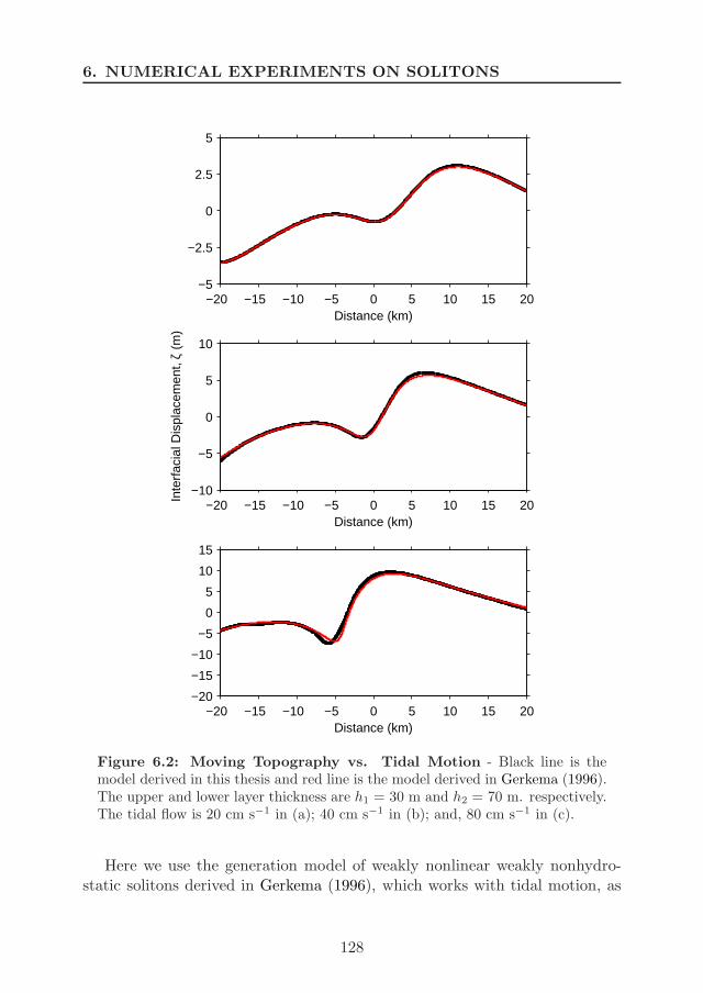
6. NUMERICAL EXPERIMENTS ON SOLITONS
−20 −15 −10 −5 0 5 10 15 20−20
−15
−10
−5
0
5
10
15
Distance (km)
−20 −15 −10 −5 0 5 10 15 20−5
−2.5
0
2.5
5
Distance (km)
−20 −15 −10 −5 0 5 10 15 20−10
−5
0
5
10
Inte
rfac
ial D
ispl
acem
ent,
ζ (m
)
Distance (km)
Figure 6.2: Moving Topography vs. Tidal Motion - Black line is themodel derived in this thesis and red line is the model derived in Gerkema (1996).The upper and lower layer thickness are h1 = 30 m and h2 = 70 m. respectively.The tidal flow is 20 cm s−1 in (a); 40 cm s−1 in (b); and, 80 cm s−1 in (c).
Here we use the generation model of weakly nonlinear weakly nonhydro-static solitons derived in Gerkema (1996), which works with tidal motion, as
128
6.2 Configuration of the Numerical Experiments
a benchmark for testing our fully nonlinear weakly nonhydrostatic generationmodel of solitons, which works with moving topography. The comparison isobviosuly not straightforward as both models are of different nature, weaklyand strongly nonlinear effects already make them different. For this reasonwe focus only on comparing the response of the model over the top of thetopography, where the ficticious forces may become important and the inter-nal tide is generated. Any differences which may appear far away from thegeneration area are indeed expected due to different nonlinear effects actingin every model. Also for this reason we present the results centred only overthis area and under weakly nonlinear settings in order to make them morecomparable (the matter here is to test that the height of the topography isnot a problem).
For clarity on the results we use for this comparison the same configuration1
we use for the numerical experiments that we will present throughout thechapter. Thus, Figure 6.2 suggests that an internal tide generated with arelatively small moving topography is equivalent to that generated via a tidalflow over topography.
6.2.4 Set of Experiments
The model operates with equations in nondimensinal form; however, we presentresults from the numerical experiments after dimensionalisation.
To organize the presentation of the numerical experiments, we chose aconfiguration which we keep fixed for most of the simulations. For simplicityon the magnitudes, we set a total water depth of 100 m (h = 100) with theparameters for the thickness of the upper and lower layers being h1 = 30 andh2 = 70 (the upper layer being thinner than the lower layer).
Regarding the topography, the height of the sill was set at 40 m with de-cresing amplitude covering mainly the interval from -10 km to 10 km overthe x-axis, thus b1 = 40 and b2 = 10000. Furthermore, the horizontal oscilla-tion of the moving topography (forcing) is always of semidiurnal fequency. Thestrength of the stratification at the interface was set by a value of g′ = 0.01 m s−2.For this configuration, the small parameter δ retaining weak nonhydrostaticeffects keeps the same value of δ = 1.67e-06.
1See following subsection for details.
129
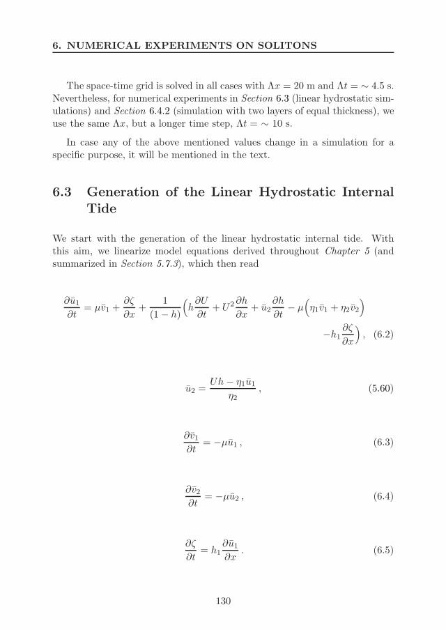
6. NUMERICAL EXPERIMENTS ON SOLITONS
The space-time grid is solved in all cases with Λx = 20 m and Λt = ∼ 4.5 s.Nevertheless, for numerical experiments in Section 6.3 (linear hydrostatic sim-ulations) and Section 6.4.2 (simulation with two layers of equal thickness), weuse the same Λx, but a longer time step, Λt = ∼ 10 s.
In case any of the above mentioned values change in a simulation for aspecific purpose, it will be mentioned in the text.
6.3 Generation of the Linear Hydrostatic InternalTide
We start with the generation of the linear hydrostatic internal tide. Withthis aim, we linearize model equations derived throughout Chapter 5 (andsummarized in Section 5.7.3), which then read
∂u1
∂t= µv1 +
∂ζ
∂x+
1
(1 − h)
(h
∂U
∂t+ U2 ∂h
∂x+ u2
∂h
∂t− µ
(η1v1 + η2v2
)
−h1∂ζ
∂x
), (6.2)
u2 =Uh − η1u1
η2, (5.60)
∂v1
∂t= −µu1 , (6.3)
∂v2
∂t= −µu2 , (6.4)
∂ζ
∂t= h1
∂u1
∂x. (6.5)
130
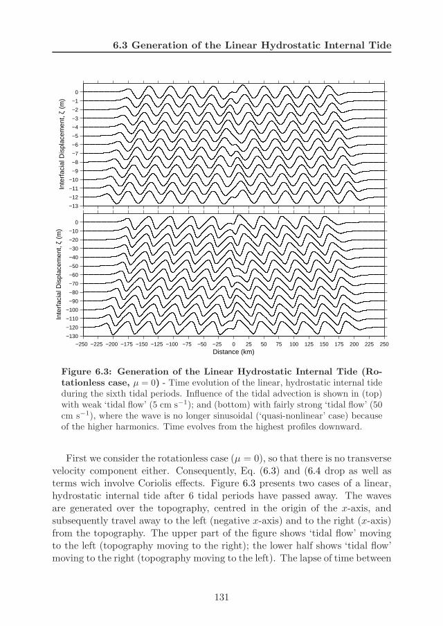
6.3 Generation of the Linear Hydrostatic Internal Tide
−13
−12
−11
−10
−9
−8
−7
−6
−5
−4
−3
−2
−1
0
Inte
rfac
ial D
ispl
acem
ent,
ζ (m
)
−250 −225 −200 −175 −150 −125 −100 −75 −50 −25 0 25 50 75 100 125 150 175 200 225 250
−130
−120
−110
−100
−90
−80
−70
−60
−50
−40
−30
−20
−10
0
Inte
rfac
ial D
ispl
acem
ent,
ζ (m
)
Distance (km)
Figure 6.3: Generation of the Linear Hydrostatic Internal Tide (Ro-tationless case, µ = 0) - Time evolution of the linear, hydrostatic internal tideduring the sixth tidal periods. Influence of the tidal advection is shown in (top)with weak ‘tidal flow’ (5 cm s−1); and (bottom) with fairly strong ‘tidal flow’ (50cm s−1), where the wave is no longer sinusoidal (‘quasi-nonlinear’ case) becauseof the higher harmonics. Time evolves from the highest profiles downward.
First we consider the rotationless case (µ = 0), so that there is no transversevelocity component either. Consequently, Eq. (6.3) and (6.4 drop as well asterms wich involve Coriolis effects. Figure 6.3 presents two cases of a linear,hydrostatic internal tide after 6 tidal periods have passed away. The wavesare generated over the topography, centred in the origin of the x-axis, andsubsequently travel away to the left (negative x-axis) and to the right (x-axis)from the topography. The upper part of the figure shows ‘tidal flow’ movingto the left (topography moving to the right); the lower half shows ‘tidal flow’moving to the right (topography moving to the left). The lapse of time between
131
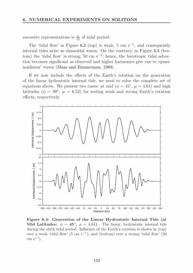
6. NUMERICAL EXPERIMENTS ON SOLITONS
sucessive representations is 112 of tidal period.
The ‘tidal flow’ in Figure 6.3 (top) is weak, 5 cm s−1, and consequentlyinternal tides arise as sinusoidal waves. On the contrary, in Figure 6.3 (bot-tom) the ‘tidal flow’ is strong, 50 cm s−1; hence, the barotropic tidal advec-tion becomes significant as observed and higher harmonics give rise to ‘quasi-nonlinear’ waves (Maas and Zimmerman, 1989).
If we now include the effects of the Earth’s rotation on the generationof the linear hydrostatic internal tide, we need to solve the complete set ofequations above. We present two cases: at mid (φ = 45, µ = 4.61) and highlatitudes (φ = 90, µ = 6.52) for testing weak and strong Earth’s rotationeffects, respectively.
−1
−0.75
−0.5
−0.25
0
0.25
0.5
0.75
1
Inte
rfac
ial D
ispl
acem
ent,
ζ (m
)
−250 −225 −200 −175 −150 −125 −100 −75 −50 −25 0 25 50 75 100 125 150 175 200 225 250
−10
−7.5
−5
−2.5
0
2.5
5
7.5
10
Inte
rfac
ial D
ispl
acem
ent,
ζ (m
)
Distance (km)
Figure 6.4: Generation of the Linear Hydrostatic Internal Tide (atMid Latitudes: φ = 45, µ = 4.61) - The linear, hydrostatic internal tideduring the sixth tidal period. Influence of the Earth’s rotation is shown in (top)over a weak ‘tidal flow’ (5 cm s−1); and (bottom) over a strong ‘tidal flow’ (50cm s−1).
132
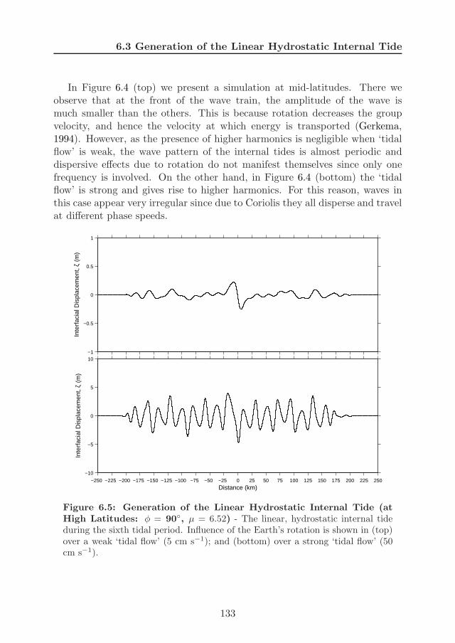
6.3 Generation of the Linear Hydrostatic Internal Tide
In Figure 6.4 (top) we present a simulation at mid-latitudes. There weobserve that at the front of the wave train, the amplitude of the wave ismuch smaller than the others. This is because rotation decreases the groupvelocity, and hence the velocity at which energy is transported (Gerkema,1994). However, as the presence of higher harmonics is negligible when ‘tidalflow’ is weak, the wave pattern of the internal tides is almost periodic anddispersive effects due to rotation do not manifest themselves since only onefrequency is involved. On the other hand, in Figure 6.4 (bottom) the ‘tidalflow’ is strong and gives rise to higher harmonics. For this reason, waves inthis case appear very irregular since due to Coriolis they all disperse and travelat different phase speeds.
−1
−0.5
0
0.5
1
Inte
rfac
ial D
ispl
acem
ent,
ζ (m
)
−250 −225 −200 −175 −150 −125 −100 −75 −50 −25 0 25 50 75 100 125 150 175 200 225 250
−10
−5
0
5
10
Inte
rfac
ial D
ispl
acem
ent,
ζ (m
)
Distance (km)
Figure 6.5: Generation of the Linear Hydrostatic Internal Tide (atHigh Latitudes: φ = 90, µ = 6.52) - The linear, hydrostatic internal tideduring the sixth tidal period. Influence of the Earth’s rotation is shown in (top)over a weak ‘tidal flow’ (5 cm s−1); and (bottom) over a strong ‘tidal flow’ (50cm s−1).
133
6. NUMERICAL EXPERIMENTS ON SOLITONS
In Figure 6.5 we increase the effects of Coriolis dispersion moving our two-fluid system to high latitudes. In the (top) simulation, the linear hydrostaticinternal tide cannot propagate away from the generation point (Gerkema,1994) and we can only appreciate tiny irregular waves doing so (note the changein vertical scale). They are due to the presence of small higher harmonicstogether with the basic linear hydrostatic internal tide. In the limit case of ainfinitesimal ‘tidal flow’, higher harmonics are completely absent and no wavesignal can propagate. In Figure 6.5 (bottom) the ‘tidal flow’ is again strongbut Coriolis dispersion too; furthermore, the induced semidiurnal barotropicflow is subinertial at high latitudes (90) so that only higher harmonics canpropagate.
6.4 Generation of Strongly Nonlinear Solitons
In this section we solve numerically the full set of equations derived in pre-vious chapter and summarized in Section 5.7.3. The main target is now toshow the generation and evolution of strongly nonlinear solitons under criticalconditions of strongly nonlinearity [as has been observed in the ocean, e. g.Stanton and Ostrovsky (1998)] in which classical KdV-type theories are notlonger applicable due to quadratic nonlinearity effects vanishes.
Firstly we focus on the generation of ‘table-top’ solitons using exactly thesame configuration as in previous simulations but now increasing the forcingto a ‘tidal flow’ of 80 cm s−1. Secondly we explore the generation of solitons atthe critical configuration of a two-fluid system in which both layers are of equalthickness. Again we force the internal tides with a ‘tidal flow’ of 80 cm s−1.
6.4.1 ‘Table-Top’ Solitons (Rotationless Test, µ = 0)
Figures 6.6 and 6.7 present the strongly nonlinear disintegration of an internaltide into ‘table-top’ solitons. On one hand, Figure 6.6 shows the generation ofa long internal tide of about 30 km wavelength which, at a first stage, splitsup into two different groups of rank-ordered solitons: a train of depresionson the leading edge; and a train of elevations, after the former packet, withinitially smaller amplitudes (Figure 6.6a). As the tidal period passes, weobserve that in the same internal tide as previous the largest elevations havenow reached the smaller depressions in the train and three leading solitons at
134

6.4 Generation of Strongly Nonlinear Solitons
the front present almost equal amplitudes around 20 m at the end of the 8th
tidal period (Figure 6.6b).
−30 −25 −20 −15 −10 −5 0
−20−15−10−5
05
10
−65 −60 −55 −50
−25−20−15−10−5
05
10
Inte
rfac
ial D
ispl
acem
ent,
ζ (m
)
−140 −130 −120 −110 −100 −90
−25−20−15−10−5
05
10
−220 −210 −200 −190 −180 −170 −160 −150
−25−20−15−10−5
05
10
Distance (km)
Figure 6.6: Generation of ‘Table-Top’ Solitons - Strongly nonlinear disin-tegration of the internal tide. (a) Generation of an internal tide at the beginningof the 8th tidal period. (b) Same disintegrated internal tide as in (a) but at theend of the 8th tidal period. (c) and (d) Disintegrated internal tides propagatingaway from the generation area. The results correspond to a simulation of 8 tidalperiods forced with a ‘tidal flow’ of 80 cm s−1.
Previous wave packets of solitons propagating away the generation areaare shown in Figures 6.6c, d corresponding to preceding disintegrated internaltides also at the end of the 8th tidal period. The ‘table-top’ soliton observed atthe leading edge of every preceding internal tide emerged in all cases from thefirst of the three solitons described previously for the front of an earlier stage ofdisintegration of the internal tide (Figure 6.6b). Once that soliton at the frontstarts to grow up and reach its maximum amplitude, it also starts to broaden
135
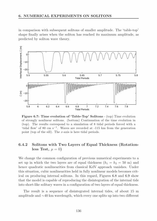
6. NUMERICAL EXPERIMENTS ON SOLITONS
in comparison with subsequent solitons of smaller amplitude. The ‘table-top’shape finally arises when the soliton has reached its maximum amplitude, aspredicted by soliton wave theory.
5.5 5.55 5.6 5.65 5.7 5.75 5.8
−20
−10
0
Inte
rfac
ial D
ispl
acem
ent,
ζ (m
)
Tidal Periods
5.8 6 6.2 6.4 6.6 6.8 7 7.2 7.4 7.6 7.8
−20
−10
0
ζ (m
)
Tidal Periods
Figure 6.7: Time evolution of ‘Table-Top’ Solitons - (top) Time evolutionof strongly nonlinear solitons. (bottom) Continuation of the time evolution in(top). The results correspond to a simulation of 8 tidal periods forced with a‘tidal flow’ of 80 cm s−1. Waves are recorded at -115 km from the generationpoint (top of the sill). The x-axis is here tidal periods.
6.4.2 Solitons with Two Layers of Equal Thickness (Rotation-less Test, µ = 0)
We change the common configuration of previous numerical experiments to aset up in which the two layers are of equal thickness (h1 = h2 = 50 m) andhence quadratic nonlinearities from classical KdV approach vanishes. Underthis situation, cubic nonlinearities held in fully nonlinear models becomes crit-ical on producing internal solitons. In this regard, Figures 6.8 and 6.9 showthat the model is capable of reproducing the disintegration of the internal tideinto short-like solitary waves in a configuration of two layers of equal thickness.
The result is a sequence of disintegrated internal tides, of about 15 mamplitude and ∼40 km wavelength, which every one splits up into two different
136

6.4 Generation of Strongly Nonlinear Solitons
packets of rank-ordered solitons: elevations of up to 5 m amplitude all alongthe crest of the main body of the internal tide; and depressions along its sine(at this stage the largest one is observed to be overpassing the small elevationsof the train of waves in the crest).
−200 −195 −190 −185 −180 −175 −170 −165 −160 −155 −150 −145 −140 −135 −130 −125−10
−5
0
5
10
Inte
rfac
ial D
ispl
acem
ent,
ζ (m
)
Distance (km)
Figure 6.8: Generation of Solitons between Two Layers of Equal Thick-ness - Nonlinear disintegration of the internal tides propagating along the inter-face of two layers of equal thickness (h1 = h2 = 50m). The waves respond to asimulation of 10 tidal periods forced with a fairly strong ‘tidal flow’ (80 cm s−1).
7 7.2 7.4 7.6 7.8 8 8.2 8.4 8.6 8.8 9−10
−5
0
5
10
ζ (m
)
Tidal Periods
Figure 6.9: Time evolution of Solitons between Two Layers of EqualThickness - Time evolution of solitons propagating along the interface of twolayers of equal thickness (h1 = h2 = 50m). The waves respond to a simulationof 10 tidal periods forced with a fairly strong ‘tidal flow’ (80 cm s−1). Waves arerecorded at -115 km from the generation point (top of the sill). The x-axis ishere tidal periods.
6.4.3 Strongly Nonlinear Solitons dispersed by the Effects ofthe Earth’s Rotation
Figure 6.10 presents a simulation of strongly nonlinear disintegration of aninternal tide at mid-latitudes (φ = 45, µ = 4.61) recorded at -50 km (top)
137
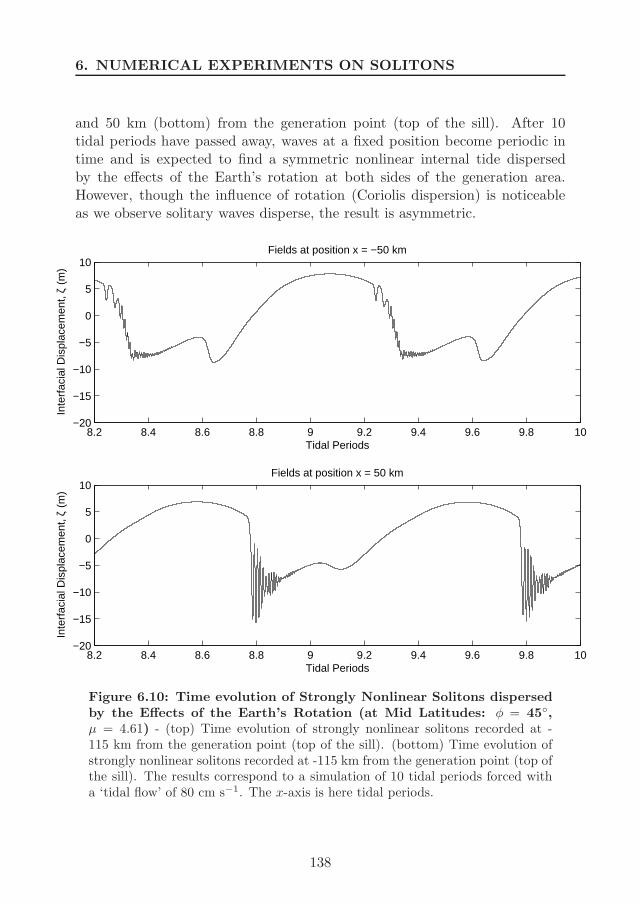
6. NUMERICAL EXPERIMENTS ON SOLITONS
and 50 km (bottom) from the generation point (top of the sill). After 10tidal periods have passed away, waves at a fixed position become periodic intime and is expected to find a symmetric nonlinear internal tide dispersedby the effects of the Earth’s rotation at both sides of the generation area.However, though the influence of rotation (Coriolis dispersion) is noticeableas we observe solitary waves disperse, the result is asymmetric.
8.2 8.4 8.6 8.8 9 9.2 9.4 9.6 9.8 10−20
−15
−10
−5
0
5
10Fields at position x = −50 km
Inte
rfac
ial D
ispl
acem
ent,
ζ (m
)
Tidal Periods
8.2 8.4 8.6 8.8 9 9.2 9.4 9.6 9.8 10−20
−15
−10
−5
0
5
10Fields at position x = 50 km
Inte
rfac
ial D
ispl
acem
ent,
ζ (m
)
Tidal Periods
Figure 6.10: Time evolution of Strongly Nonlinear Solitons dispersedby the Effects of the Earth’s Rotation (at Mid Latitudes: φ = 45,µ = 4.61) - (top) Time evolution of strongly nonlinear solitons recorded at -115 km from the generation point (top of the sill). (bottom) Time evolution ofstrongly nonlinear solitons recorded at -115 km from the generation point (top ofthe sill). The results correspond to a simulation of 10 tidal periods forced witha ‘tidal flow’ of 80 cm s−1. The x-axis is here tidal periods.
138

6.5 Conclusions
This situation responds to the fact that the model is initialised with anasymmetric forcing, i. e. fluid at rest and topography moving to the right.This generates an asymmetry in the response of the model which in a rotatingsimulation is conserved in time over the top of the topography (conservation ofpotential vorticity) and is advected to leftward/rightward propagating waves;hence, the appearance in the results of asymmetric strongly nonlinear internaltides dispersed by Coriolis. This is supported when initialising the modelwith the fluid at rest and the topography moving to the left, the result we haveobtained is equally asymmetric producing a mirrored image to Figure 6.10 (themirrored image is not shown here). This demonstrates that the asymmetryreally stems from the initial conditions and does not lie in our model equationsas such, which are symmetric with respect to left and right.
Obviously, this asymmetry becomes smaller when the initial ‘tidal flow’ isweak and therefore the generated asymmetry is small as well.
6.5 Conclusions
In the previous chapter we derived a new model including full nonlinearity, asin Choi & Canmassa (1999), but with the added features of Coriolis dispersion,topography, and a forcing mechanism of internal tides.
The results of this chapter validate the model as a useful tool for exploringand interpreting the conditions under which full nonlinearity effects becomeimportant for soliton generation and a fully nonlinear set of equations needto be considered to study the phenomenon. In particular, this is the case fortable-top solitons and appearance of nonlinearity in a two-layer system withequal layer thickness.
Future work should extend these calculations to make a comparison withfield observations.
139

6. NUMERICAL EXPERIMENTS ON SOLITONS
140
Chapter 7
Conclusions and FutureResearch
In this chapter the main conclusions and scientific contributions of the thesisare summarized. Additionally, we also suggest where further research in thefuture may benefit the understanding of the phenomena we are dealing here.
I Breeze-forced oscillations
1 Results from a rotary wavelet analysis indicate that diurnal wind forc-ing (sea-land breezes) in the Gulf of Cadiz and the Gulf of Valenciaenhances clockwise current oscillations (breeze-forced motions) duringspring-summer months, contributing greatly to the near-inertial en-ergy budget and its seasonal variability. The diurnal-inertial currentvariance has been estimated to be an order of magnitude higher thanestimated variance during winter months. These results support therole of breeze-forced oscillations on the generation and accumulationof near-inertial energy within the critical latitudes for diurnal-inertialresonance.
2 Results from a rotary wavelet analysis indicate that clockwise cur-rent oscillations in the Cape Penas area are enhanced during summermonths; however, the increase of inertial current variance is not as largeas has been estimated for the Gulf of Cadiz and the Gulf of Valencia.
141
7. CONCLUSIONS AND FUTURE RESEARCH
This mainly responds to the Cape Penas area is out of the criticallatitudes for diurnal-inertial resonance.
3 An analysis on diapycnal mixing processes associated to breeze-forcedoscillations, within the critical latitudes for resonance (Bay of Setubal),shows evidence of an enhancement of diurnal-inertial energy availableto promote vertical mixing in stratified and vertically sheared flowswith subcritical values of Ri. This research also suggests that theremay exist an internal control on the strength of the ocean response tobreeze forcing due to the deepening and smoothing of the pycnoclinedriven by diapycnal mixing processes.
4 Future Research: Further analysis of time series data (currents, temper-ature and salinity) covering the total water depth in combination withco-located and simultaneous wind data would greatly benefit the un-derstanding of how breeze-forced oscillations evolve in time and space,with special attention to the role that associated diapycnal mixing maybe playing on the vertical structure of these forced-motions. In thisregard, we also find that measurements of the turbulent kinetic energydissipation rate with a coastal turbulence microprofiler would help onthe assessment of the diapycnal mixing processes promoted by breeze-forced oscillations.
II Strongly nonlinear tide-generated internal solitons
1 A new model for the study of strongly nonlinear tide-generated internalsolitons has been derived including full nonlinearity, Coriolis dispersion,topography, and a forcing mechanism of internal tides.
2 Numerical experiments validate the model as a useful tool for exploringand interpreting the conditions under which full nonlinearity effects be-come important for soliton generation and a fully nonlinear set of equa-tions need to be considered to study the phenomenon. In particular,this is the case for table-top solitons and appearance of nonlinearity ina two-layer system with equal layer thickness.
3 Future Research: Further analysis should extend these calculations tomake a comparison with field observations.
142
Appendix A
Rotary Wavelet Method
The programs we use to apply the rotary wavelet method are based on mod-ifications made by Hormazabal et al. (2004) to the original wavelet soft-ware (http://paos.colorado.edu/research/wavelets/) provided by Torrence andCompo (1998).
The content of this appendix is for the most part borrowed from AppendixA in Hormazabal et al. (2004) and Torrence and Compo (1998), though ithas been summarized and adapted to be focused on the requirements of ourresearch.
A.1 Rotary Wavelet Power Spectrum
The rotary wavelet power spectrum measures the time series variance of a vec-tor at each period and each time for both the positive (counterclockwise) andnegative (clockwise) rotation components. Starting from a complex discretetime series xn = un + ivn with zero mean, constant time spacing δt, and timeindex n = 0, ..., N − 1, the discrete Fourier transform develops as
x(ωk) =1
N
N−1∑
n=0
xne−iωknδt k = 0, ..., N − 1, (A.1)
143

A. ROTARY WAVELET METHOD
where N is the number of time steps in the time series, k is the frequencyindex, and ωk is the angular frequency, which is defined as
ωk =
2πkNδt k ≤ N
2 ,
− 2πkNδt k > N
2 .
(A.2)
These positive (+ωk) and negative (−ωk) frequencies correspond to twodimensional vectors rotating counterclockwise (CCW) and clockwise (CW),respectively, at the frequency |ωk| Gonella (1972). To separate both signalsin time-frequency space, we need a wavelet function able to capture boththe positive and negative oscillations of the time series as separate peaks inwavelet power. We use the derivative of a Gaussian (DOG) wavelet whoseFourier transform (of the normalized function) is
Ψ(sωk) =(2πs
δt
) 12 −im√
Γ(m + 0.5)(sωk)
me−(sωk)2
2 m = 6, (A.3)
where√
2πs/δt is the factor that normalizes the wavelets (what ensure atotal energy of unity), Γ is the gamma function, m is the derivative of the DOGwavelet function, and s is the wavelet scale, which is related to Fourier periodthrough the relation λ = 2πs/
√m + 0.5 (Table 1 in Torrence and Compo
(1998)).
Next, in order to obtain the CCW and CW wavelet transform in Fourierspace, we separate positive and negative frequencies. For a given scale s andtime nδt the continuos wavelet transform is defined as the inverse discreteFourier transform of a product of Fourier transforms. Then, we have theCCW wavelet transform given by
W+n (s) =
N−1∑
k=0
x(ωk)Ψ∗(sωk)e
iωknδt Ψ∗(sωk) = 0 ωk < 0, (A.4)
and, the CW wavelet transform given by
144
A.2 Rotary Coefficient
W−
n (s) =
N−1∑
k=0
x(ωk)Ψ∗(sωk)e
iωknδt Ψ(sωk) = 0 ωk > 0 . (A.5)
where the asterisk indicates the complex conjugate. Then, the rotarywavelet power spectra of the counterclockwise and clockwise components areobtained by multiplying each wavelet transform by its corresponding complexconjugate
S+n (s) = W+
n (s)W+∗
n (s) ωk ≥ 0, (A.6)
S−
n (s) = W−
n (s)W−∗
n (s) ωk ≤ 0. (A.7)
The total wavelet power spectrum is defines as Sn(s) = S+n (s) + S−
n (s).
A.2 Rotary Coefficient
The rotation finally exhibited by the vector (counterclockwise or clockwise)is determined by the component containing the largest magnitude for a givenfrequency and time. If both components have equal magnitude, then themotions are rectilinear. As for rotary spectral analysis, the rotary coefficientcan be defined as
rn(s) =S+
n (s) − S−n (s)
S+n (s) + S−
n (s)(A.8)
and ranges from rn(s) = +1 for a CCW gyre to rn(s) = −1 for a CW gyre,and over rn(s) = 0 for unidirectional motion (Emery and Thomson, 1998).
145
A. ROTARY WAVELET METHOD
A.3 Statistical Significance Test
The null hypothesis for the significance of a peak in the wavelet power spec-trum is defined (Torrence and Compo, 1998) as follows. We assume that thetime series has a mean power spectrum given by a red or white noise back-ground spectrum associated with the wavelet power spectrum. Whether apeak in the wavelet power spectrum is significantly above this backgroundspectrum, it can be assumed that peak is a true feature with a certain percentconfidence. For clarity, the reader should notice that ‘significant at the 5%level’ is equivalent to the ‘95% confidence level ’ and involves a test againsta certain background level. And, the ‘95% confidence interval ’ refers to therange of confidence about a given value.
We model the wavelet transform for each scale and all times as a lag-1autoregressive process to develop a statistical significance test for the waveletpower spectrum (Torrence and Compo, 1998). A simple model for red noiseis the univariate lag-1 autoregressive [AR(1), or Markov] process:
xn = αxn−1 + zn, (A.9)
where α is the assumed lag-1 autocorrelation, x0 = 0, and zn is taken fromGaussian white noise. Application of Gilman et al. (1963) leads to the red orwhite noise background spectrum associated with the wavelet power spectrumat a given time and scale following
Pk =1 − α2
1 + α2 − 2αcos(2πk/N), (A.10)
where k = 0N/2 is the frequency index; α = (α1 +√
α2)/2; and, α1 andα2 are the lag-1 and lag-2 complex autocorrelations, respectively. Hence, bychoosing an appropriate lag-1 autocorrelation, one can use eq. (A.10) to modeleither a red-noise spectrum, or a white noise spectrum if α = 0. In ourresearch, we use the red noise background spectrum.
Next, the wavelet power spectrum distribution at each time n and scale sis given by
146
A.4 Cross-Rotary Wavelet Power Spectrum
Sn(s)
σ2∼ 1
2Pkχ
22, (A.11)
where the wavelet power spectrum is chi-square distributed with 2 degreesof freedom.
A.4 Cross-Rotary Wavelet Power Spectrum
The rotary wavelet analysis implies a separation of the vector time series fora specified period (scale) and time into CCW- and CW-rotating components.Hence, application of this analysis to two different vector time series whichwere measured simultaneously allow us to determine the similarity betweenthe two times series in terms of their CW and CCW components in time-frequency space.
Thus, the corotating cross-rotary wavelet spectrum provides an estimate ofthe joint energy contained by two time series for rotating components in thesame direction (e.g., the CW component of x with the CW component of y).With this objective, we define a set of corotating functions which provide thisestimate.
Given two complex time series x and y with rotary wavelet transform W±xn
and W±yn , where n is the time index, s is the scale, and ± represents a posi-
tive (CCW) and negative (CW) component, respectively, the corotating cross-wavelet spectrum follows
S±xyn (s) = W±x
n W±y∗n . (A.12)
A.5 Rotary Wavelet Coherence Squared Spectrum
The corotating wavelet coherence measures the correlation between rotarycomponents of two different vector time series which are rotating in the samedirection as a function of period (scale) and time. The coherence takes positive
147
A. ROTARY WAVELET METHOD
values 0 ≤ ±γ2n(s) ≤ 1 whereby coherences near zero indicate a negligible rela-
tionship between corotating components, while coherences near unity indicatea high degree of similarity.
The corotating coherence squared, ±γ2n(s), between the rotary component
of two different vector time series measured simultaneously, is given by
±γ2n(s) =
|⟨s−1S±xy
n (s)⟩|2
⟨s−1S±x
n (s)⟩⟨
s−1S±yn (s)
⟩ , (A.13)
where 〈 〉 indicates smoothing in time and scale, and the factor s−1 convertsthe wavelet power to energy density. The smoothing for the complex cross-wavelet spectrum is performed separately for the real and imaginary parts.
The wavelet function provides a natural width of the smoothing func-tion (Torrence and Webster, 1999). For time smoothing, the filter is providedby a Gaussian function exp[−(nδt/s)2/2], defined for each scale and normal-ized to have unit weight. For the scale smoothing, the filter width is given bythe scale decorrelation length of the wavelet we are using. In our case we useDOG (m = 6), for which the scale is 0.97 (see Table 2 in Torrence and Compo(1998)). The scale smoothing is done using a triangle filter.
A.6 Rotary Wavelet Phase Spectrum
The corotating wavelet phase shows any lag or lead relationship between coro-tating components of two different vector time series measured simultaneouslyas a function of period and time. The corotating wavelet phase between posi-tive (CCW) or negative (CW) components is defined as
φ±
n (s) = tan−1I
[⟨s−1S±xy
n (s)]⟩
R
[⟨s−1S±xy
n (s)]⟩ , (A.14)
148

A.6 Rotary Wavelet Phase Spectrum
where R is the real, and I is the imaginary part of the smoothed, corotatingcross-wavelet spectrum 1.
1As for corotating cross-wavelet spectrum, we can define counterrotating functions forcross spectrum, coherence, and phase, which provide an estimate of the joint energy, cor-relation, and difference of phase between rotary components that are rotating in oppositedirections (e.g., between the CW component of x and the CCW component of y). However,in this thesis, we only deal with corotating wavelet analysis.
149

A. ROTARY WAVELET METHOD
150
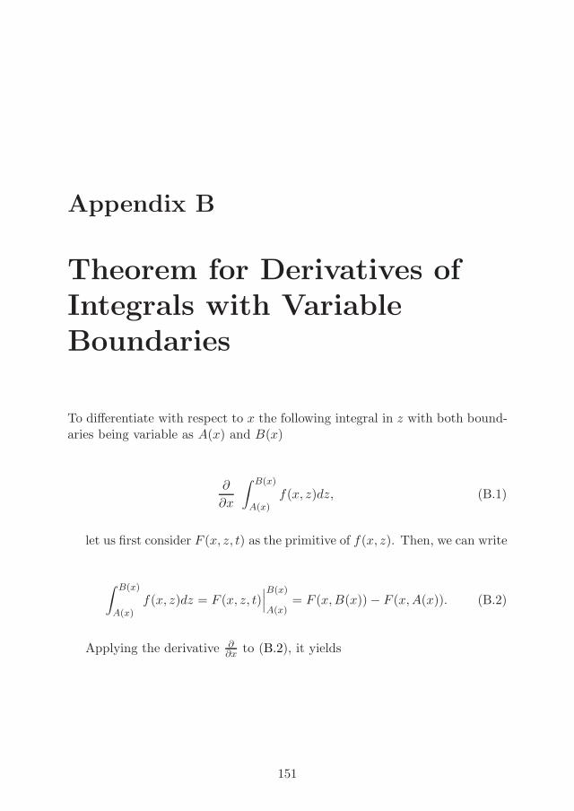
Appendix B
Theorem for Derivatives ofIntegrals with VariableBoundaries
To differentiate with respect to x the following integral in z with both bound-aries being variable as A(x) and B(x)
∂
∂x
∫ B(x)
A(x)f(x, z)dz, (B.1)
let us first consider F (x, z, t) as the primitive of f(x, z). Then, we can write
∫ B(x)
A(x)f(x, z)dz = F (x, z, t)
∣∣∣B(x)
A(x)= F (x,B(x)) − F (x,A(x)). (B.2)
Applying the derivative ∂∂x to (B.2), it yields
151
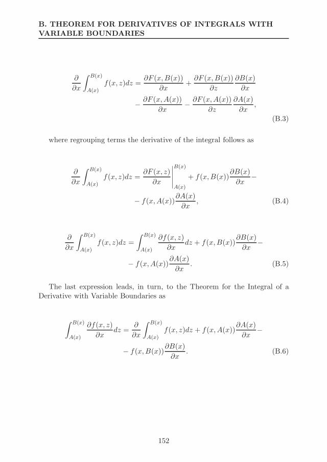
B. THEOREM FOR DERIVATIVES OF INTEGRALS WITHVARIABLE BOUNDARIES
∂
∂x
∫ B(x)
A(x)f(x, z)dz =
∂F (x,B(x))
∂x+
∂F (x,B(x))
∂z
∂B(x)
∂x
− ∂F (x,A(x))
∂x− ∂F (x,A(x))
∂z
∂A(x)
∂x,
(B.3)
where regrouping terms the derivative of the integral follows as
∂
∂x
∫ B(x)
A(x)f(x, z)dz =
∂F (x, z)
∂x
∣∣∣∣∣
B(x)
A(x)
+ f(x,B(x))∂B(x)
∂x−
− f(x,A(x))∂A(x)
∂x, (B.4)
∂
∂x
∫ B(x)
A(x)f(x, z)dz =
∫ B(x)
A(x)
∂f(x, z)
∂xdz + f(x,B(x))
∂B(x)
∂x−
− f(x,A(x))∂A(x)
∂x. (B.5)
The last expression leads, in turn, to the Theorem for the Integral of aDerivative with Variable Boundaries as
∫ B(x)
A(x)
∂f(x, z)
∂xdz =
∂
∂x
∫ B(x)
A(x)f(x, z)dz + f(x,A(x))
∂A(x)
∂x−
− f(x,B(x))∂B(x)
∂x. (B.6)
152
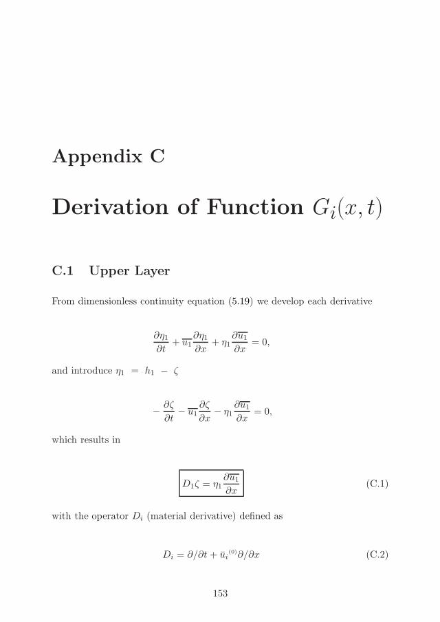
Appendix C
Derivation of Function Gi(x, t)
C.1 Upper Layer
From dimensionless continuity equation (5.19) we develop each derivative
∂η1
∂t+ u1
∂η1
∂x+ η1
∂u1
∂x= 0,
and introduce η1 = h1 − ζ
− ∂ζ
∂t− u1
∂ζ
∂x− η1
∂u1
∂x= 0,
which results in
D1ζ = η1∂u1
∂x(C.1)
with the operator Di (material derivative) defined as
Di = ∂/∂t + ui(0)∂/∂x (C.2)
153
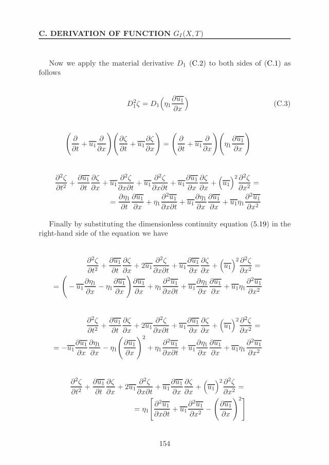
C. DERIVATION OF FUNCTION GI(X,T )
Now we apply the material derivative D1 (C.2) to both sides of (C.1) asfollows
D21ζ = D1
(η1
∂u1
∂x
)(C.3)
(∂
∂t+ u1
∂
∂x
)(∂ζ
∂t+ u1
∂ζ
∂x
)
=
(∂
∂t+ u1
∂
∂x
)(
η1∂u1
∂x
)
∂2ζ
∂t2+
∂u1
∂t
∂ζ
∂x+ u1
∂2ζ
∂x∂t+ u1
∂2ζ
∂x∂t+ u1
∂u1
∂x
∂ζ
∂x+(u1
)2 ∂2ζ
∂x2=
=∂η1
∂t
∂u1
∂x+ η1
∂2u1
∂x∂t+ u1
∂η1
∂x
∂u1
∂x+ u1η1
∂2u1
∂x2
Finally by substituting the dimensionless continuity equation (5.19) in theright-hand side of the equation we have
∂2ζ
∂t2+
∂u1
∂t
∂ζ
∂x+ 2u1
∂2ζ
∂x∂t+ u1
∂u1
∂x
∂ζ
∂x+(u1
)2 ∂2ζ
∂x2=
=
(− u1
∂η1
∂x− η1
∂u1
∂x
)∂u1
∂x+ η1
∂2u1
∂x∂t+ u1
∂η1
∂x
∂u1
∂x+ u1η1
∂2u1
∂x2
∂2ζ
∂t2+
∂u1
∂t
∂ζ
∂x+ 2u1
∂2ζ
∂x∂t+ u1
∂u1
∂x
∂ζ
∂x+(u1
)2 ∂2ζ
∂x2=
= −u1∂u1
∂x
∂η1
∂x− η1
(∂u1
∂x
)2
+ η1∂2u1
∂x∂t+ u1
∂η1
∂x
∂u1
∂x+ u1η1
∂2u1
∂x2
∂2ζ
∂t2+
∂u1
∂t
∂ζ
∂x+ 2u1
∂2ζ
∂x∂t+ u1
∂u1
∂x
∂ζ
∂x+(u1
)2 ∂2ζ
∂x2=
= η1
[∂2u1
∂x∂t+ u1
∂2u1
∂x2−(
∂u1
∂x
)2]
154

C.2 Lower Layer Over an Oscillating Topography
whence we obtain the second material derivative of ζ in terms of the func-tion G1(x, t)
∂2ζ
∂t2+
∂u1
∂t
∂ζ
∂x+ 2u1
∂2ζ
∂x∂t+ u1
∂u1
∂x
∂ζ
∂x+(u1
)2 ∂2ζ
∂x2= η1G1(x, t)
and hence
D21ζ = η1G1(x, t) (C.4)
C.2 Lower Layer Over an Oscillating Topography
Now we introduce η2 = h2 − h(x, t) + ζ into the dimensionless continuityequation (5.22) and follow the same steps as previously. Derivation follows as
∂η2
∂t+ u2
∂η2
∂x+ η2
∂u2
∂x= 0
∂ζ
∂t− ∂h
∂t+ u2
∂ζ
∂x− u2
∂h
∂x+ η2
∂u2
∂x= 0
which results in
D2ζ − D2h(x, t) = −η2∂u2
∂x
Now we apply the material derivative Di (C.2) to both sides of (C.5) asfollows
D22ζ − D2
2h(x, t) = D2
(− η2
∂u2
∂x
)
155
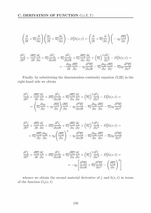
C. DERIVATION OF FUNCTION GI(X,T )
(∂
∂t+ u2
∂
∂x
)(∂ζ
∂t+ u2
∂ζ
∂x
)
− D22h(x, t) =
(∂
∂t+ u2
∂
∂x
)(
− η2∂u2
∂x
)
∂2ζ
∂t2+
∂u2
∂t
∂ζ
∂x+ u2
∂2ζ
∂x∂t+ u2
∂2ζ
∂x∂t+ u2
∂u2
∂x
∂ζ
∂x+(u2
)2 ∂2ζ
∂x2− D2
2h(x, t) =
= −∂η2
∂t
∂u2
∂x− η2
∂2u2
∂x∂t− u2
∂η2
∂x
∂u2
∂x− u2η2
∂2u2
∂x2
Finally, by substituting the dimensionless continuity equation (5.22) in theright-hand side we obtain
∂2ζ
∂t2+
∂u2
∂t
∂ζ
∂x+ 2u2
∂2ζ
∂x∂t+ u2
∂u2
∂x
∂ζ
∂x+(u2
)2 ∂2ζ
∂x2− D2
2h(x, t) =
=
(
u2∂η2
∂x+ η2
∂u2
∂x
)∂u2
∂x− η2
∂2u2
∂x∂t− u2
∂η2
∂x
∂u2
∂x− u2η2
∂2u2
∂x2
∂2ζ
∂t2+
∂u2
∂t
∂ζ
∂x+ 2u2
∂2ζ
∂x∂t+ u2
∂u2
∂x
∂ζ
∂x+(u2
)2 ∂2ζ
∂x2− D2
2h(x, t) =
= u2∂u2
∂x
∂η2
∂x+ η2
(∂u2
∂x
)2
− η2∂2u2
∂x∂t− u2
∂η2
∂x
∂u1
∂x− u2η2
∂2u2
∂x2
∂2ζ
∂t2+
∂u2
∂t
∂ζ
∂x+ 2u2
∂2ζ
∂x∂t+ u2
∂u2
∂x
∂ζ
∂x+(u2
)2 ∂2ζ
∂x2− D2
2h(x, t) =
= −η2
[∂2u2
∂x∂t+ u2
∂2u2
∂x2−(
∂u2
∂x
)2]
whence we obtain the second material derivative of ζ and h(x, t) in termsof the function G2(x, t)
156
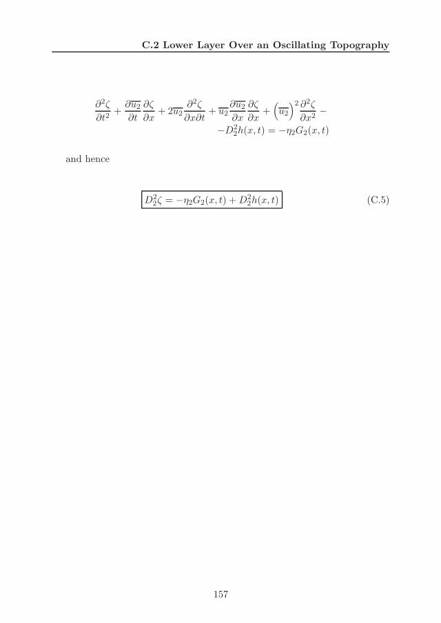
C.2 Lower Layer Over an Oscillating Topography
∂2ζ
∂t2+
∂u2
∂t
∂ζ
∂x+ 2u2
∂2ζ
∂x∂t+ u2
∂u2
∂x
∂ζ
∂x+(u2
)2 ∂2ζ
∂x2−
−D22h(x, t) = −η2G2(x, t)
and hence
D22ζ = −η2G2(x, t) + D2
2h(x, t) (C.5)
157

C. DERIVATION OF FUNCTION GI(X,T )
158

Appendix D
Derivation of(
∂p′2(1)
∂x
)
Starting from the initial expression
(∂p′2(1)
∂x
)=
[(h2 − h)
∂G2
∂x− ∂h
∂xG2 −
∂
∂x(D2
2h)] 1
η2
∫ ζ
−h2+hdz z
+1
2
∂G2
∂x
1
η2
∫ ζ
−h2+hdz z2 +
∂h
∂xζG2 − η2
∂ζ
∂xG2
−([h2 − h]ζ + ζ2/2)∂G2
∂x+
∂ζ
∂xD2
2h + ζ∂
∂x(D2
2h)
(D.1)we develop the integral and obtain
(∂p′2(1)
∂x
)=
[(h2 − h)
∂G2
∂x− ∂h
∂xG2 −
∂
∂x(D2
2h)] 1
2η2
(ζ2 − [−h2 + h]2
)
+∂G2
∂x
1
6η2
(ζ3 − [−h2 + h]3
)
+∂h
∂xζG2 − η2
∂ζ
∂xG2 − ([h2 − h]ζ + ζ2/2)
∂G2
∂x+
∂ζ
∂xD2
2h
+ζ∂
∂x(D2
2h)
=[(h2 − h)
∂G2
∂x− ∂h
∂xG2 −
∂
∂x(D2
2h)]12(ζ − h2 + h)
+∂G2
∂x
1
6
(ζ2 + ζ(−h2 + h) + (−h2 + h)2
)
+∂h
∂xζG2 − η2
∂ζ
∂xG2 − ([h2 − h]ζ + ζ2/2)
∂G2
∂x+
∂ζ
∂xD2
2h
+ζ∂
∂x(D2
2h)
(D.2)
159
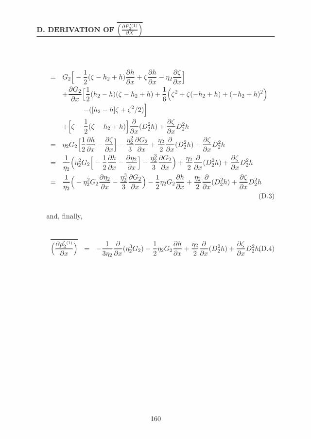
D. DERIVATION OF(
∂P ′
2(1)
∂X
)
= G2
[− 1
2(ζ − h2 + h)
∂h
∂x+ ζ
∂h
∂x− η2
∂ζ
∂x
]
+∂G2
∂x
[12(h2 − h)(ζ − h2 + h) +
1
6
(ζ2 + ζ(−h2 + h) + (−h2 + h)2
)
−([h2 − h]ζ + ζ2/2)]
+[ζ − 1
2(ζ − h2 + h)
] ∂
∂x(D2
2h) +∂ζ
∂xD2
2h
= η2G2
[12
∂h
∂x− ∂ζ
∂x
]− η2
2
3
∂G2
∂x+
η2
2
∂
∂x(D2
2h) +∂ζ
∂xD2
2h
=1
η2
(η22G2
[− 1
2
∂h
∂x− ∂η2
∂x
]− η3
2
3
∂G2
∂x
)+
η2
2
∂
∂x(D2
2h) +∂ζ
∂xD2
2h
=1
η2
(− η2
2G2∂η2
∂x− η3
2
3
∂G2
∂x
)− 1
2η2G2
∂h
∂x+
η2
2
∂
∂x(D2
2h) +∂ζ
∂xD2
2h
(D.3)
and, finally,
(∂p′2(1)
∂x
)= − 1
3η2
∂
∂x(η3
2G2) −1
2η2G2
∂h
∂x+
η2
2
∂
∂x(D2
2h) +∂ζ
∂xD2
2h.(D.4)
160
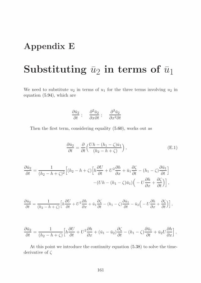
Appendix E
Substituting u2 in terms of u1
We need to substitute u2 in terms of u1 for the three terms involving u2 inequation (5.94), which are
∂u2
∂t;
∂2u2
∂x∂t;
∂3u2
∂x2∂t
Then the first term, considering equality (5.60), works out as
∂u2
∂t=
∂
∂t
(Uh − (h1 − ζ)u1
(h2 − h + ζ)
), (E.1)
∂u2
∂t=
1
(h2 − h + ζ)2
[(h2 − h + ζ)
[h
∂U
∂t+ U2 ∂h
∂x+ u1
∂ζ
∂t− (h1 − ζ)
∂u1
∂t
]
−(Uh − (h1 − ζ)u1)(− U
∂h
∂x+
∂ζ
∂t
)],
∂u2
∂t=
1
(h2 − h + ζ)
[h
∂U
∂t+ U2 ∂h
∂x+ u1
∂ζ
∂t− (h1 − ζ)
∂u1
∂t− u2
(− U
∂h
∂x+
∂ζ
∂t
)],
∂u2
∂t=
1
(h2 − h + ζ)
[h
∂U
∂t+ U2 ∂h
∂x+ (u1 − u2)
∂ζ
∂t− (h1 − ζ)
∂u1
∂t+ u2U
∂h
∂x
],
At this point we introduce the continuity equation (5.38) to solve the time-derivative of ζ
161

E. SUBSTITUTING U2 IN TERMS OF U1
∂u2
∂t=
1
η2
[h
∂U
∂t+ U2 ∂h
∂x+ (u1 − u2)
(η1
∂u1
∂x− u1
∂ζ
∂x
)− η1
∂u1
∂t+ u2U
∂h
∂x
]
resulting the first term in (E.1) as
∂u2
∂t= −η1
η2
∂u1
∂t+
1
η2
[h
∂U
∂t+ U2 ∂h
∂x+ (u1 − u2)
(η1
∂u1
∂x− u1
∂ζ
∂x
)+ u2U
∂h
∂x
](E.2)
For simplicity we define here the variable φ as
r =1
η2
[h
∂U
∂t+ U2 ∂h
∂x+ (u1 − u2)
(η1
∂u1
∂x− u1
∂ζ
∂x
)+ u2U
∂h
∂x
](E.3)
leading to
∂u2
∂t= −η1
η2
∂u1
∂t+ φ (E.4)
and being φ a variable to be added on the right-hand side of equation(5.110) when substituting u2 in terms of u1 on its left-hand side.
Analogously, the second term in (E.1) involves
∂2u2
∂x∂t=
∂2
∂x∂t
(Uh − (h1 − ζ)u1
(h2 − h + ζ)
)(E.5)
what is the same as applying ∂∂x to (E.4) following
∂2u2
∂x∂t= −η1
η2
∂2u1
∂x∂t− ∂(η1/η2)
∂x
∂u1
∂t+
∂φ
∂x
(E.6)
162
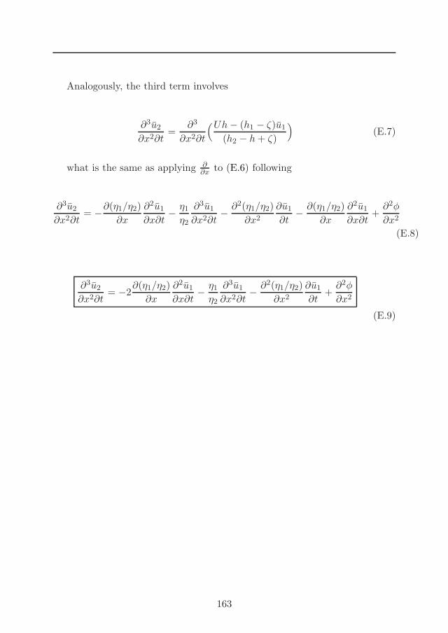
Analogously, the third term involves
∂3u2
∂x2∂t=
∂3
∂x2∂t
(Uh − (h1 − ζ)u1
(h2 − h + ζ)
)(E.7)
what is the same as applying ∂∂x to (E.6) following
∂3u2
∂x2∂t= −∂(η1/η2)
∂x
∂2u1
∂x∂t− η1
η2
∂3u1
∂x2∂t− ∂2(η1/η2)
∂x2
∂u1
∂t− ∂(η1/η2)
∂x
∂2u1
∂x∂t+
∂2φ
∂x2
(E.8)
∂3u2
∂x2∂t= −2
∂(η1/η2)
∂x
∂2u1
∂x∂t− η1
η2
∂3u1
∂x2∂t− ∂2(η1/η2)
∂x2
∂u1
∂t+
∂2φ
∂x2
(E.9)
163

E. SUBSTITUTING U2 IN TERMS OF U1
164
References
Aguiar-Gonzalez, B., Rodrıguez-Santana, A., Cisneros-Aguirre, J., Martınez-Marrero, A., 2011. Diurnal-inertial motions and diapycnal mixing on thePortuguese shelf. Cont. Shelf Res. 31 (11), 1193–1201.
Akylas, T., Grimshaw, R., Clarke, S., Tabaei, A., 2007. Reflecting tidal wavebeams and local generation of solitary waves in the ocean thermocline. J.Fluid Mech. 593, 297–314.
Alford, M., 2003a. Reply to comment by F. Feser et al. on Improved globalmaps and 54-year history of wind-work on ocean inertial motions. Geophys.Res. Lett. 30 (22), 2166.
Alford, M. H., 2003b. Redistribution of energy available for ocean mixing bylong-range propagation of internal waves. Nature 423, 159–162.
Allard, R., Dykes, J., Hsu, Y. L., Kaihatu, J., Conley, D., 2008. A real-timenearshore wave and current prediction system. J. Mar. Syst. 69, 37–58.
Aparna, M., Shetye, S., Shankar, D., Shenoi, S., Mehra, P., Desai, R., 2005.Estimating the seaward extent of sea breeze from QuikSCAT scatterometry.Geophys. Res. Lett. 32 (13), L13601.
Apel, J., 2002. An Atlas of Oceanic Internal Solitary Waves: Oceanic InternalWaves and Solitnons.
Apel, J. R., Holbrook, J. R., Liu, A. K., Tsai, J. J., 1985. The Sulu Sea internalsoliton experiment. J. Phys. Oceanogr. 15 (12), 1625–1651.
Apel, J. R., Ostrovsky, L. A., Stepanyants, Y. A., Lynch, J. F., 2006. Internalsolitons in the ocean. Tech. rep., Woods Hole Oceanographic Institution.
Battisti, D., Clarke, A., 1982. A simple method for estimating barotropic tidalcurrents on continental margins with specific application to the M2 tide offthe Atlantic and Pacific coasts of the United States. J. Phys. Oceanogr. 12,8–16.
165
REFERENCES
Bogucki, D., Dickey, T., Redekopp, L., 1997. Sediment resuspension and mix-ing by resonantly generated internal solitary waves. J. Phys. Oceanogr.27 (7), 1181–1196.
Butman, B., Alexander, P. S., Scotti, A., Beardsley, R. C., Anderson, S. P.,2006. Large internal waves in Massachusetts Bay transport sediments off-shore. Cont. Shelf Res. 26 (17), 2029–2049.
Chaigneau, A., Pizarro, O., Rojas, W., 2008. Global climatology of near-inertial current characteristics from Lagrangian observations. Geophys. Res.Lett. 35.
Chen, C., Reid, R., Nowlin, W., 1996. Near-inertial oscillations over the Texas-Louisiana shelf. J. Geophys. Res. 101, 3509–3524.
Chen, C., Xie, L., 1997. A numerical study of wind-induced, near-inertial oscil-lations over the Texas-Louisiana shelf. J. Geophys. Res. 102 (C7), 15583–15.
Choi, W., Camassa, R., 1999. Fully nonlinear internal waves in a two-fluidsystem. J. Fluid Mech. 396 (1-36), 1–36.
Coelho, E. F., Robinson, A. R., 2003. NATO tactical ocean modeling: themini-HOPS strategy in the Maritime Rapid Environmental Assessment 2003Sea Trial. In: MREP03 Proceedings, NATO Undersea Research Centre. pp.CP–47/CD–70.
Craig, P., 1989a. A model of diurnally forced vertical current structure near30 latitude. Cont. Shelf Res. 9 (11), 965–980.
Craig, P., 1989b. Constant-eddy-viscosity models of vertical structure forcedby periodic winds. Cont. Shelf Res. 9 (4), 343–358.
Criado-Aldeanueva, F., Garcıa-Lafuente, J., Navarro, G., Ruiz, J., 2009. Sea-sonal and interannual variability of the surface circulation in the easternGulf of Cadiz (SW Iberia). J. Geophys. Res. 114 (C1).
Da Silva, J., New, A.L..and Magalhaes, J., 2009. Internal solitary waves in theMozambique Channel: Observations and interpretation. J. Geophys. Res.114 (C5), C05001.
da Silva, J. C., New, A., Azevedo, A., 2007. On the role of SAR for observing”local generation” of internal solitary waves off the Iberian Peninsula. Can.J. Rem Sens. 33 (5), 388–403.
166
REFERENCES
De Mesquita, A., Harari, J., 2003. On the harmonic constants of tides andtidal currents of the South-eastern brazilian shelf. Cont. Shelf Res. 23 (11),1227–1237.
DiMarco, S., Howard, M., Reid, R., 2000. Seasonal variation of wind-drivendiurnal current cycling on the Texas–Louisiana continental shelf. Geophys.Res. Lett. 27, 1017–1020.
Djordjevic, V. D., Redekopp, L., 1978. The fission and disintegration of in-ternal solitary waves moving over two-dimensional topography. J. Phys.Oceanogr. 8 (6), 1016–1024.
Durran, D., 1999. Numerical methods for wave equations in geophysical fluiddynamics. Vol. 32. Springer Verlag.
Emery, W., Thomson, R., 1998. Data Analysis Methods in Physical Oceanog-raphy. Pergamon.
Farmer, D., Armi, L., 1999. Stratified flow over topography: the role of small-scale entrainment and mixing in flow establishment. Proceedings of theRoyal Society of London. Series A: Mathematical, Physical and EngineeringSciences 455 (1989), 3221–3258.
Font, J., Garcıa-Ladona, E., Gorriz, E., 1995. The seasonality of measoscalemotion in the North Channel of the western Mediterranean: several yearsof evidence. Oceanologica Acta 18, 207–219.
Fu, L. L., 1981. Observations and models of inertial waves in the deep ocean.Rev. Geophys. Space Phys. 19, 141–170.
Furevik, T., Foldvik, A., 1996. Stability at M 2 critical latitude in the BarentsSea. J. Geophys. Res. 101, 8823–8837.
Garret, C., 2001. What is the ‘Near-Inertial’ Band and Why Is It Differentfrom the Rest of the Internal Wave Spectrum? J. Phys. Oceanogr. 31, 962–971.
Gerkema, T., 1994. Nonlinear dispersive internal tides: generation models fora rotating ocean. Ph.D. thesis, Utrecht University.
Gerkema, T., 1996. A unified model for the generation and fission of internaltides in a rotating ocean. J. Mar. Res. 54 (3), 421–450.
167

REFERENCES
Gerkema, T., 2001. Internal and interfacial tides: beam scattering and localgeneration of solitary waves. J. Mar. Res. 59 (2), 227–255.
Gerkema, T., Shrira, V. I., 2005. Near-inertial waves in the ocean: beyond the‘traditional approximation’. J. Fluid Mech. 529, 195–219.
Gerkema, T., Zimmerman, J., 1995. Generation of nonlinear internal tides andsolitary waves. J. Phys. Oceanogr. 25 (6), 1081–1094.
Gerkema, T., Zimmerman, J., 2008. An introduction to internal waves. Vol.119.
Gerkema, T., Zimmerman, J., Maas, L., van Haren, H., 2008. Geophysical andastrophysical fluid dynamics beyond the traditional approximation. Rev.Geophys. 46 (2).
Gill, A., 1984. On the behavior of internal waves in the wakes of storms. J.Phys. Oceanogr. 14 (7), 1129–1151.
Gille, S., Smith, S., Lee, S., 2003. Measuring the sea breeze from QuikSCATScatterometry. Geophys. Res. Lett. 30 (3), 1114.
Gille, S., Smith, S., Statom, N., 2005. Global observations of the land breeze.Geophys. Res. Lett. 32 (5), L05605.
Gilman, D., Fuglister, F., Mitchell Jr, J., 1963. On the power spectrum of rednoise. J. Atmos. Sci. 20 (2), 182–184.
Gonella, J., 1972. A rotary-component method for analyzing meteorologicaland oceanographic vector time series. Deep-Sea Res. 19, 833–846.
Grimshaw, R.H.J..and Smyth, N., 1986. Resonant flow of a stratified fluid overtopography. J. Fluid Mech. 169, 429–464.
Grimshaw, R., Ostrovsky, L., Shrira, V., Stepanyants, Y. A., 1998. Long non-linear surface and internal gravity waves in a rotating ocean. Surv. Geophys.19 (4), 289–338.
GrimShaw, R., PelinovSky, E., Poloukhina, O., 2002. Higher-order Korteweg-de Vries models for internal solitary waves in a stratified shear flow with afree surface. Nonlinear Proc. Geoph. 9 (3/4), 221–235.
168
REFERENCES
Grimshaw, R., Pelinovsky, E., Talipova, T., 1997. The modified Korteweg-deVries equation in the theory of large-amplitude internal waves. NonlinearProc. Geoph. 4 (4), 237–250.
Grimshaw, R., Pelinovsky, E., Talipova, T., Kurkin, A., 2004. Simulation ofthe transformation of internal solitary waves on oceanic shelves. J. Phys.Oceanogr. 34 (12), 2774–2791.
Haley, P., Lermusiaux, P., 2010. Multiscale two-way embedding schemes forfree-surface primitive equations in the Multidisciplinary Simulation, Esti-mation and Assimilation System. Oc. Dynam. 60 (6), 1497–1537.
Halpern, D., 1977. Description of wind and of upper ocean current and temper-ature variations on the continental shelf off northwest Africa during Marchand April 197. J. Phys. Oceanogr. 7, 422.
Hayashi, Y., 1979. Space-Time Spectral Analysis of Rotary Vector Series. J.Atmos. Sci. 36 (5), 757–766.
Helfrich, K., Grimshaw, R., 2008. Nonlinear disintegration of the internal tide.J. Phys. Oceanogr. 38 (3), 686–701.
Helfrich, K. R., Melville, W. K., 2006. Long nonlinear internal waves. Annu.Rev. Fluid Mech. 38, 395–425.
Hormazabal, S., Shaffer, G., Leth, O., 2004. Coastal transition zone off Chile.J. Geophys. Res. 109 (C01021).
Hormazabal, S., Shaffer, G., Pizarro, O., 2002. Tropical Pacific control ofintraseasonal oscillations off Chile by way of oceanic and atmospheric path-ways. Geophys. Res. Lett. 29 (6), 1081.
Hunter, E., Chant, R., Bowers, L., Glenn, S., Kohut, J., 2007. Spatial andtemporal variability of diurnal wind forcing in the coastal ocean. Geophys.Res. Lett. 34 (3), L03607.
Hyder, P., Simpson, J., Xing, J., Gille, S., 2011. Observations over an annualcycle and simulations of wind-forced oscillations near the critical latitudefor diurnal-inertial resonance. Cont. Shelf Res.
Hyder, P., Simpson, J. H., Christopoulos, S., 2002. Sea-breeze forced diurnalsurface currents in the Thermaikos Gulf, North-west Aegean. Cont. ShelfRes. 22, 585–601.
169
REFERENCES
Jarosz, E., Hallock, Z., Teague, W., 2007. Near-inertial currents in the DeSotoCanyon region. Cont. Shelf Res. 27 (19), 2407–2426.
Jo, T.-C., Choi, W., 2002. Dynamics of strongly nonlinear internal solitarywaves in shallow water. Stud. Appl. Math. 109 (3), 205–227.
Kakutani, T., Yamasaki, N., 1978. Solitary waves on a two-layer fluid. J. Phys.Soc. Japan 45 (2), 674–679.
Kaplan, D., Largier, J., Botsford, L., 2005. HF radar observations of surfacecirculation off Bodega Bay (northern California, USA). J. Geophys. Res.110, C10020.
Kaplan, D., Largier, J., Navarrete, S., Guinez, R., Castilla, J., 2003. Largediurnal temperature fluctuations in the nearshore water column. Estuar.Coast. Shelf Sci. 57 (3), 385–398.
Keen, C., Lyons, W., 1978. Lake/land breeze circulations on the western shoreof Lake Michigan. J. Appl. Meteor. 17 (12), 1843–1855.
Knight, P. J., Howarth, M. J., Rippeth, T. P., 2002. Inertial currents in thenorthern North sea. J. Sea Res. 47, 269–284.
Ko, D., Martin, P., Rowley, C., Preller, R., 2008. A real-time coastal oceanprediction experiment for MREA04. J. Mar. Syst. 69 (1-2), 17–28.
Koop, C. G., Butler, G., 1981. An investigation of internal solitary waves. J.Fluid Mech. 112, 225–251.
Korteweg, D., de Vries, G., 1895. XLI. On the change of form of long wavesadvancing in a rectangular canal, and on a new type of long stationarywaves. The London, Edinburgh, and Dublin Philosophical Magazine andJournal of Science 39 (240), 422–443.
Kunze, E., 1985. Near-Inertial Wave Propagation in Geostrophic Shear. J.Phys. Oceanogr. 15, 544–565.
Kunze, E., Boss, E., 1998. A Model for Vortex-Trapped Internal Waves. J.Phys. Oceanogr. 28, 2104–2115.
Lam, F., Haley Jr, P., Janmaat, J., Lermusiaux, P., Leslie, W., Schouten,M., te Raa, L., Rixen, M., 2009. At-sea real-time coupled four-dimensionaloceanographic and acoustic forecasts during battlespace preparation 2007.J. Mar. Syst. 78, S306–S320.
170

REFERENCES
Lamb, K. G., Yan, L., 1996. The evolution of internal wave undular bores:comparisons of a fully nonlinear numerical model with weakly nonlineartheory. Journal of physical oceanography 26 (12), 2712–2734.
Lee, C., Beardsley, R., 1974. The generation of long nonlinear internal wavesin a weakly stratified shear flow. J. Geophys. Res. 79 (3), 453–462.
Lerczak, J., Hendershott, M., Winant, C., 2001. Observations and modelingof coastal internal waves driven by a diurnal sea breeze. J. Geophys. Res.106 (19), 715–19.
Lermusiaux, P., Xu, J., Chen, C., Jan, S., Chiu, L., Yang, Y., 2010. CoupledOcean–Acoustic Prediction of Transmission Loss in a Continental Shelf-break Region: Predictive Skill, Uncertainty Quantification, and DynamicalSensitivities. IEEE Transactions, Journal of Oceanic Engineering 35 (4),895–916.
Leslie, W.G.and Robinson, A., Haley, PJ. .and Logoutov, O., Moreno, P., Ler-musiaux, P.F.J .and Coelho, E., 2008. Verification and training of real-timeforecasting of multi-scale ocean dynamics for maritime rapid environmentalassessment. J. Mar. Syst. 69 (1-2), 3–16.
Liu, A. K., Holbrook, J. R., Apel, J., 1985. Nonlinear internal wave evolutionin the Sulu Sea. J. Phys. Oceanogr. 15 (12), 1613–1624.
Logan, J. D., 1987. Applied mathematics: a contemporary approach. Wiley.
Lyons, W., 1972. The climatology and prediction of the Chicago lake breeze.J. Appl. Meteor. 11, 1259–1270.
Lyons, W., Olsson, L., 1973. Detailed Mesometeorological Studies of Air Pol-lution Dispersion in the Chicago Lake Breeze. Mon. Weather Rev. 101 (5),387–403.
Maas, L., Van Haren, J., 1987. Observations on the vertical structure of tidaland inertial currents in the central North Sea. J. Mar. Res. 45 (2), 293–318.
Maas, L., Zimmerman, J., 1989. Tide-topography interactions in a stratifiedshelf sea I. Basic equations for quasi-nonlinear internal tides. Geophys. As-trophys. Fluid Dynam. 45 (1-2), 1–35.
171

REFERENCES
Macias, D., Garcıa, C. M., Echevarrıa Navas, F., Vazquez-Lopez-Escobar, A.,Bruno Mejıas, M., 2006. Tidal induced variability of mixing processes onCamarinal Sill (Strait of Gibraltar): A pulsating event. J. Mar. Syst. 60 (1),177–192.
MacKinnon, J., Winters, K., 2005. Subtropical catastrophe: Significant lossof low-mode tidal energy at 28.9. Geophys. Res. Lett. 32 (15), L15605.
Martınez-Marrero, A., Rodrıguez-Santana, A., Hernandez-Guerra, A., Fraile-Nuez, E., Lopez-Laatzen, F., Velez-Belchı, P., Parrilla, G., 2008. Distribu-tion of water masses and diapycnal mixing in the Cape Verde Frontal Zone.Geophys. Res. Lett. 35 (7), L07609.
Martins, F., Leitao, P., Neves, R., 2002. Simulating vertical water mixing inhomogeneous estuaries: the SADO Estuary case. Hydrobiologia 475/476,221–227.
Maxworthy, T., 1979. A note on the internal solitary waves produced by tidalflow over a three-dimensional ridge. J. Geophys. Res. 84 (C1), 338–346.
Melville, W., Helfrich, K., 1987. Transcritical two-layer flow over topography.J. Fluid Mech. 178, 31–52.
Middleton, J., Denniss, T., 1993. The propagation of tides near the criticallatitude. Geophys. Astrophys. Fluid Dynam. 68 (1-4), 1–13.
Miles, J., 1986. Richardson’s criterion for the stability of stratified shear flow.Physics of Fluids 29, 3470–3471.
Millot, C., Crepon, M., 1981. Inertial Oscillations on the Continental Shelfof the Gulf of Lions - Observations and Theory. J. Phys. Oceanogr. 11,639–657.
Miyata, M., 1985. An internal solitary wave of large amplitude. La Mer 23,43–48.
Miyata, M., 1988. Long internal waves of large amplitude. In: K. Horikawa,H. M. (Ed.), Nonlinear Water Waves, IUTAM Symp., Tokyo 1987. Berlin:Springer-Verlag, pp. 399–406.
Moroz, W., 1967. A Lake Breeze on the Eastern Shore of Lake Michigan:Observations and Model. J. Atmos. Sci. 24, 337–355.
172
REFERENCES
Moum, J., Farmer, D., Smyth, W., Armi, L., Vagle, S., 2003. Structureand generation of turbulence at interfaces strained by internal solitarywaves propagating shoreward over the continental shelf. J. Phys. Oceanogr.33 (10), 2093–2112.
Muench, R. D., Padman, L., Howard, S. L., Fahrbach, E., 2002. Upper oceandiapycnal mixing in the northwestern Weddell Sea. Deep-Sea Res. II 49,4843–4861.
Munk, W., Wunsch, C., 1998. Abyssal recipes II: energetics of tidal and windmixing. Deep-Sea Res. I 45 (12), 1977–2010.
New, A., 1988. Internal tidal mixing in the Bay of Biscay. Deep-Sea Res.35 (5), 691–709.
New, A., da Silva, J., 2002. Remote-sensing evidence for the local generationof internal soliton packets in the central Bay of Biscay. Deep-Sea Res. I49 (5), 915–934.
New, A., Pingree, R., 1992. Local generation of internal soliton packets in thecentral Bay of Biscay. Deep-Sea Res. 39 (9), 1521–1534.
New, A.L..and Pingree, R., 1990. Large-amplitude internal soliton packets inthe central Bay of Biscay. Deep-Sea Res. 37 (3), 513–524.
O‘Brien, J. J., Pillsbury, R. D., 1974. Rotary Wind Spectra in a Sea BreezeRegime. J. Appl. Meteor. 13 (7), 820–825.
Orlic, M., 1987. Oscillations at the inertial period on the Adriatic Sea shelf.Cont. Shelf Res. 7, 577–598.
Osborne, A., Burch, T., 1980. Internal solitons in the Andaman Sea. Science208 (4443), 451–460.
Ostrovsky, L., Stepanyants, Y. A., 1989. Do internal solitions exist in theocean? Rev. Geophys. 27 (3), 293–310.
Pacanowski, R. C., Philander, S. G. H., 1981. Parameterization of VerticalMixing in Numerical Models of Tropical Oceans. J. Phys. Oceanogr. 11,1443–1451.
Park, J., Kim, K., King, B., 2005. Global statistics of inertial motions. Geo-phys. Res. Lett. 32 (14), L14612.
173
REFERENCES
Pattiaratchi, C., Hegge, B., Gould, J., Eliot, I., 1997. Impact of sea-breezeactivity on nearshore and foreshore processes in southwestern Australia.Cont. Shelf Res. 17, 1539–1560.
Pawlowicz, R., Beardsley, B., Lentz, S., 2002. Classical tidal harmonic analy-sis including error estimates in MATLAB using T TIDe. Comput. Geosci.28 (8), 929–937.
Pelegrı, J. L., Sangra, P., 1998. A mechanism for layer formation in stratifiedgeophysical flows. J. Geophys. Res. 103 (30), 679–693.
Pidgeon, E., Winant, C., 2005. Diurnal variability in currents and temperatureon the continental shelf between central and southern California. J. Geophys.Res. 110, C03024.
Pielke, R., Segal, M., 1986. Mesoscale circulations forced by differential terrainheating. Mesoscale Meteorology and Forecasting, 516–548.
Pingree, R., Mardell, G., 1985. Solitary internal waves in the Celtic Sea. Prog.Oceanogr. 14, 431–441.
Pinkel, R., 2000. Internal solitary waves in the warm pool of the westernequatorial Pacific. J. Phys. Oceanogr. 30 (11), 2906–2926.
Pinones, A., Valle-Levinson, A., Narvaez, D., Vargas, C., Navarrete, S., Yuras,G., Castilla, J., 2005. Wind-induced diurnal variability in river plume mo-tion. Estuar. Coast. Shelf Sci. 65 (3), 513–525.
Pollard, R., 1970. On the generation by winds of inertial waves in the ocean.Deep-Sea Res. 17 (4), 795–812.
Pollard, R., 1980. Properties of near-surface inertial oscillations. J. Phys.Oceanogr. 10 (3), 385–398.
Pollard, R. T., Millard, R. C., 1970. Comparison between observed and simu-lated wind-generated inertial oscillations. Deep-Sea Res. 17, 813–821.
Poulain, P., 1990. Near-inertial and diurnal motions in the trajectories ofmixed layer drifters. J. Mar. Res. 48 (4), 793–823.
Qi, H., De Szoeke, R., Paulson, C., Eriksen, C., 1995. The structure of near-inertial waves during ocean storms. Collections.
174
REFERENCES
Reynolds-Fleming, J., Luettich Jr, R., 2004. Wind-driven lateral variability ina partially mixed estuary. Estuar. Coast. Shelf Sci. 60 (3), 395–407.
Rippeth, T. P., Simpson, J. H., Player, R. J., Garcia, M., 2002. Currentoscillations in the diurnal-inertial band on the Catalonian shelf in spring.Cont. Shelf Res. 22, 247–265.
Rixen, M., Ferreira-Coelho, E., 2007. Operational surface drift prediction usinglinear and non-linear hyper-ensemble statistics on atmospheric and oceanmodels. J. Mar. Syst. 65, 105–121.
Rodrıguez-Santana, A., Pelegrı, J. L., Sangra, P., Marrero-Dıaz, A., 1999.Diapycnal mixing in Gulf Stream meanders. J. Geophys. Res. 104, 25891–25912.
Rodrıguez-Santana, A., Pelegrı, J. L., Sangra, P., Marrero-Dıaz, A., 2001. Onthe relevance of diapycnal mixing for the stability of frontal meanders. Sci.Mar. 65 (Suppl. 1), 259–267.
Rosenfeld, L., 1988. Diurnal period wind stress and current fluctuations overthe continental shelf off northern California. J. Geophys. Res. 93 (C3), 2257–2276.
Russell, J., 1838a. Report on waves. In: Murray, J. (Ed.), Report of the 14thMeeting of British Association for the Advancement of Science. pp. 311–390.
Russell, J., 1838b. Report to committee on waves. In: Murray, J. (Ed.), Reportof the 7th Meeting of British Association for the Advancement of Science.pp. 417–496.
Salat, J., Tintore, J., Font, J., Wang, D.-P., Vieira, M., 1992. Near-Inertial Mo-tion on the Shelf-Slope Front off Northeast Spain. J. Geophys. Res. 97 (C5),7277–7281.
Sandstrom, H., Elliott, J., 1984. Internal tide and solitons on the Scotian Shelf:A nutrient pump at work. J. Geophys. Res. 89 (C4), 6415–6426.
Sangra, P., Basterretxea, G., Pelegrı, J. L., Arıstegui, J., 2001. Chlorophyllincrease due to internal waves in the shelf-break of Gran Canaria Island(Canary Islands). Sci. Mar. 65 (Suppl. 1), 89–97.
Schahinger, R. B., 1988. Near-inertial motions on the South Australian shelf.J. Phys. Oceanogr. 18, 492–504.
175
REFERENCES
Sills, D., 1998. Lake and land breezes in southwestern Ontario: observations,analyses and numerical modelling. Ph.D. thesis, York University.
Simionato, C., , Meccia, V., Dragani, W. Nunez, M., 2005. Barotropic tide andbaroclinic waves observations in the Rıo de la Plata Estuary. J. Geophys.Res. 110, C06008.
Simmons, H., Hallberg, R., Arbic, B., 2004. Internal wave generation in aglobal barcolinic tide model. Deep-Sea Res. II 51, 3042–3068.
Simpson, J. E., 1994. Sea Breeze and Local Wind. Cambridge University Press,New York.
Simpson, J. H., Hyder, P., Rippeth, T. P., 2002. Forced Oscillations nearthe Critical Latitude for Diurnal-Inertial Response. J. Phys. Oceanogr. 32,177–187.
Sobarzo, M., Bravo, L., Moffat, C., 2010. Diurnal-period, wind-forced oceanvariability on the inner shelf off Concepcion, Chile. Cont. Shelf Res. 30 (20),2043–2056.
Sobarzo, M., Shearman, R. K., Lentz, S., 2007. Near-inertial motions over thecontinental shelf off Concepcion, central Chile. Prog. Oceanogr. 75, 348–362.
Stanton, T., Ostrovsky, L., 1998. Observations of highly nonlinear internalsolitons over the continental shelf. Geophys. Res. Lett. 25 (14), 2695–2698.
Tiemann, C., Worcester, P., Cornuelle, B. D., 2001. Acoustic scattering byinternal solitary waves in the Strait of Gibraltar. J. Acoust. Soc. Am. 109,143.
Torrence, C., Compo, G., 1998. A practical guide to wavelet analysis. B. Am.Meteorol. Soc. 79 (1), 61–78.
Torrence, C., Webster, P., 1999. Interdecadal changes in the ENSO-monsoonsystem. Journal of Climate 12 (8), 2679–2690.
Ueckermann, M., Lermusiaux, P., 2010. High-order schemes for 2D unsteadybiogeochemical ocean models. Oc. Dynam. 60 (6), 1415–1445.
van Aken, H. M., Maas, L. R. M., van Haren, H., 2005. Observations of InertialWave Events near the Continental Slope off Goban Spur. J. Phys. Oceanogr.35, 1329–1340.
176

REFERENCES
Van Gastel, P., Pelegrı, J. L., 2004. Estimates of gradient Richardson numbersfrom vertically smoothed data in the Gulf Stream region. Scientia Marina68 (4), 459–482.
van Haren, H., 2000. Properties of vertical current shear across stratication inthe North Sea. J. Mar. Res. 58, 465–491.
Van Haren, H., 2005. Tidal and near-inertial peak variations around the diur-nal critical latitude. Geophys. Res. Lett. 32 (23), L23611.
van Haren, H., 2007. Longitudinal and topographic variations in North At-lantic tidal and inertial energy around latitudes 30±10 N. J. Geophys. Res.112 (C10), C10020.
van Haren, H., Maas, L., Zimmerman, J. T. F., Ridderinkhof, H., Malschaert,H., 1999. Strong inertial currents and marginal internal wave stability inthe central North Sea. Geophys. Res. Lett. 26, 2993–2996.
Wang, D., Lermusiaux, P., Haley, P., Eickstedt, D., Leslie, W., Schmidt, H.,2009. Acoustically focused adaptive sampling and on-board routing for ma-rine rapid environmental assessment. J. Mar. Syst. 78, S393–S407.
Watanabe, M., Hibiya, T., 2002. Global estimates of the wind-induced energyflux to inertial motions in the surface mixed layer. Geophys. Res. Lett.29 (8), 1239.
Webster, F., 1968. Observation of inertial period motions in the deep sea. Rev.Geophys. 6, 473–490.
Xu, Z., Yin, B., 2012. Oceanography. InTech, Ch. Variability of Internal Soli-tary Waves in the Northwest South China Sea.
Young, W. R., Ben Jelloul, M., 1997. Propagation of near-inertial oscillationsthrough a geostrophic flow. J. Mar. Res. 55, 735–766.
Zavialov, P., Moller Jr, O., Campos, E., 2002. First direct measurements ofcurrents on the continental shelf of Southern Brazil. Cont. Shelf Res. 22 (14),1975–1986.
Zeng, K., Alpers, W., 2004. Generation of internal solitary waves in the SuluSea and their refraction by bottom topography studied by ERS SAR imageryand a numerical model. Int. J. Remote Sens. 25 (7-8), 1277–1281.
177

REFERENCES
Zhang, X., DiMarco, S., Smith IV, D., Howard, M., Jochens, A., Hetland, R.,2009. Near-resonant ocean response to sea breeze on a stratified continentalshelf. J. Phys. Oceanogr. 39 (9), 2137–2155.
Zhang, X., Smith IV, D., DiMarco, S., Hetland, R., 2010. A numerical studyof sea-breeze-driven ocean Poincare wave propagation and mixing near thecritical latitude. J. Phys. Oceanogr. 40 (1), 48–66.
178

Data Acknowledgements
It is not always needed to count with new data for making new research. Onecould think it may be straightforward to get success on presenting somethingnew when one makes use of untouched data, but open public data and datarecycled from previous projects (even when they were planned with differenttargets) are also a fruitful source of information always ready for refreshinginsights and challenging research.
The first half of this PhD study has been developed following that philoso-phy with the support of Puertos del Estado (Spain), the Instituto Hidrografico- Portugal and the NATO Undersea Research Centre (NURC), which allowedthe use of the data we present.
Hence, I want to thank Puertos del Estado (Spain) for his efficient andkind service on providing the public data which are the base of the researchin Chapter 2. Likewise, I thank Dr. Jesus Cisneros Aguirre and the NATOUndersea Research Centre (NURC) for permitting the use of the data collectedduring the MREA04 sea trial; as well as the Instituto Hidrografico - Portugalfor providing wind data from a land meteorological station at Sines. Theyform the core of the work reported in Chapter 3.
The second half of this PhD study was greatly benefited thanks to thekindness of Dr. Theo Gerkema, who provided me from the beginning withhis numerical code for the generation of nonlinear dispersive interfacial tidesand solitary waves on the f -plane (Gerkema, 1996). I cannot imagine a betterstarting point for the numerical code we developed in this thesis.
179

180
Agradecimientos
Este trabajo ha crecido bajo la mirada complice de personas muy especiales.Es el momento de darles las gracias. Algunos nombres se repetiran, diferentesson los motivos y los lugares, e incluso los idiomas. Intentare mantener unorden, pero lo que ahora se presenta me voy a permitir el capricho de dejarque fluya y oscile con su perıodo particular, el mıo. Estoy convencido que loentenderan...
La presente Tesis Doctoral ha sido dirigida por el Dr. Angel Rodrıguez San-tana (Universidad de Las Palmas de Gran Canaria - ULPGC), el Dr. TheoGerkema (Royal Netherlands Institute for Sea Research - NIOZ) y el Dr. JesusCisneros Aguirre (Universidad de Las Palmas de Gran Canaria - ULPGC), aquienes agradezco la confianza y dedicacion que me han brindado durante es-tos anos de mi etapa de formacion como investigador. Aprecio enormementeel tiempo que habeis dedicado a guiar este trabajo con vuestra valiosa experi-encia.
Me encuentro tambien agradecido al Dr. Samuel Hormazabal de la Univer-sidad Catolica de Valparaıso, cuyo contribucion a mi trabajo de investigacionha sido muy importante. Gracias por tu dedicacion y generosa hospitalidad.Este trabajo se ha nutrido tambien de la experiencia del Dr. Antonio MartınezMarrero, quien siempre mostro interes y encontro tiempo para atender mis du-das.
Dentro del Grupo de Investigacion OFYGA, del cual he formado partedurante mi etapa como doctorando en la ULPGC, quiero tambien agradecera la Dra. Angeles Marrero Dıaz su dedicacion y atencion conmigo, siem-pre disponible para ayudar. No podıa ser de otro modo, dentro del GrupoOFYGA, agradezco muy especialmente a Angel y a Jesus su continuado in-teres en mi formacion, en mi presente y en mi futuro, siempre dispuestos aofrecerme nuevas oportunidades, participacion en campanas oceanograficas,contactos con otros centros de investigacion, etc ... ¡Gracias!
Al Dr. Josep Lluıs Pelegrı, al Dr. Pablo Sangra Inciarte y al Dr. MiguelBruno Mejıas quisiera agradecer su confianza al permitirme la oportunidadde participar en varias campanas oceanograficas a su cargo. En todas ellas laexperiencia vivida fue siempre enriquecedora.
Durante mis anos de doctorado tuve la generosa oportunidad de colaborarcon la Dra. May Gomez y el Dr. Ted Packard, gracias por contar conmigo en
181
Agradecimientos
vuestra investigacion. Ted, investigar a tu lado es un placer, tu vitalidad esinspiradora, mil gracias por contagiarme tu entusiasmo por la ciencia.
Estos anos de laboratorio no han podido contar con mejores companeros detrabajo y amigos: Monica, Francis, Carolina, Mireya, Sheila, Charles, Bego,...Compartir tiempo y espacio con ustedes ha sido un placer. No se me ocurremejor escenario para trabajar y compartir vivencias durante el dıa.
Mis inicios en la programacion con Matlab y escritura en LATEX fueronmucho mas amenos de lo que pudiera ser habitual al profano. Y eso fue graciasal tiempo que generosamente me dedico el Dr. Francisco Machın. Esta tesistiene mucho de lo que he aprendido de ti. Guardo especialmente en el recuerdoel tiempo compartido juntos en Barcelona.
Idaira, Aridane, Isis, Inma, Rosa,... estan vinculados de manera especial amis primeros anos de curiosidad oceanografica durante la carrera.
En lo que a problemas informaticos se refiere, gracias por tu ayuda Jorge,mas de un disco duro se ha salvado gracias a ti. Mis inicios en la oceanografıacon Mac tuvieron algun que otro contratiempo que rapidamente se resolviogracias a la buena disposicion y ayuda de David.
Desde que inicie la carrera en Ciencias del Mar (CCM) hasta el dıa de hoyhe compartido mis vivencias oceanograficas con muchos amigos que vienenahora a mi memoria ... es imposible nombrarlos a todos, pero no por ello dejode decirles desde aquı: gracias por estar ahı.
Desde hace mas de una decada que cuento con vuestra amistad, carino yapoyo... ¡menuda suerte!... Gracias Monica, Angela, Fede.
En el Centre Mediterrani D’Investigacions Marines i Ambientals (CMIMA-CSIC) en Barcelona realice mis cursos de Master y Doctorado en Oceanografıaa traves del programa organizado por la ULPGC. Alla el Dr. Josep LluısPelegrı em va rebre amablement durant la meva estada, oferint-me totes lesfacilitats d’acces i ubicacio al Departament d’Oceanografia Fısica per superaramb exit la meva primera etapa investigadora. Moltes Gracies Josep Lluıs!
After my stay at the CMIMA-CSIC, I travelled to The Hague (The Nether-lands) to collaborate with Dr. Frans-Peter A. Lam and Dr. Mathijs Schoutenat the Netherlands Organisation for Applied Scientific Research (TNO). Dur-ing this period I was introduced to HOPS numerical modeling. The time Ispent at TNO is unforgettable, working with both of you is one of the gifts
182

I will always remember from my PhD time. There are not enough words tothank all I received from you. I appreciated very much your advices and care-ful guide. I also thank Prof. Dr. P. F. J. Lermusiaux (Massachusetts Instituteof Technology, MIT) for his help, inputs and comments in the distance onmodeling work for MREA exercises. From my period at TNO I cannot forgetabout Benoit and Jeroen for all their help at my arrival and for the joyful timewe shared, as well as with Mathieu, Antonio, Jacqueline, Michael,...
My stays at NIOZ were possible thanks to Dr. Frans-Peter A. Lam, whofirstly introduced me to Prof. Dr. L. R. M. Maas and Dr. T. Gerkema. TheNetherlands always brings to me nice memories. My time there was special,and that was thanks to the people I met on my way. They made my stay tobe great: joyful and fruitful at the same time.
I already mentioned people from The Hague at TNO, but I also met won-derful people I want to remember in these lines at Texel during my staysat NIOZ, specially Jenny, Femke, Carola, Anna and Andrea. I also want tothank the Physical Oceanography Department at NIOZ, which kindly hostedme during my PhD time there. In this regard, I am grateful to Prof. Dr.Leo Maas, who always shared his interest on my work with refreshing andinspiring questions. At this point, it may be obvious to the reader that Ideeply feel this thesis is half spanish, half dutch. And the dutch side of thisresearch was developed thanks to Dr. Theo Gerkema. I appreciate a lot yourhospitality and all the time you have spent working with me and supervisingmy PhD study. I am also grateful for your continuous interest on helping mewith future steps: ¡Muchas Gracias por todo Theo! He aprendido y disfrutadomuchısimo trabajando a tu lado.
Angela, gracias por estar ahı siempre, por los muchos anos de amistaddesde que nos conocemos, y por todos los que vendran. Muchas gracias portu apoyo en lo personal y en lo laboral. Nuestras conferencias Gran Canaria- Texel, y luego al reves, son inolvidables... el destino es curioso, pero contigoal lado ademas de curioso es siempre agradable.
Monica, muchas son las horas que hemos compartido dentro y fuera del lab,dentro y fuera de ‘la isla’. Muchos son los grandes momentos vividos en estosanos de amistad (y los que vendran): viajes sorpresa, excursiones aventura,videoconferencias en la distancia,... Los he disfrutado y disfruto muchısimo.Muchas gracias por tu apoyo en lo personal y en lo laboral, por tu companıa,por estar ahı siempre.
183
Agradecimientos
Goonie, gracias por tirar de mi pantalon y guiar cada uno de mis pasosaquella noche de Febrero, tuviste que tirar fuerte, y en varias ocasiones, peronunca te falto fuerza a pesar de tu pequeno tamano. Estoy seguro que estasen el cielo de las pizzas y los churros.
Las primeras palabras de esta tesis van dedicadas a ellos, y de ellos es elhonor de cerrarla: mis padres Mappi e Ignacio, y mi hermano Jose. Ustedeshan hecho posible que haya llegado hasta aquı. Gracias por vuestra companıay carino. No tengo palabras para agradecerles que siempre pueda contar conustedes. Gracias por todas vuestras visitas cuando estoy fuera de ‘la isla’, mehacen sentir pieza importante en vuestra vida y siempre suponen una inyeccionde alegrıa. Mappi, gracias por explicarme ‘la teorıa del sandwich’, aplicablea todos los ambitos de la vida. Si he terminado esta tesis es gracias a quela he aplicado una vez mas. Gracias por ayudarme siempre a ver lo esencialy a encontrar mi camino. Ignacio, en momentos de estres ‘tus teorıas de lasondas’ me hicieron reır y ver alguna que otra luz, gracias por ambos efectos,llegaban siempre que hacıan falta. Jose, gracias por tus animos, por alegrartee interesarte siempre por lo que hago, por tu tiempo conmigo y por cuidarsiempre de tu ‘hermanito pequeno’ (aunque ya no sea tan pequenito aun tenecesito). ¡Gracias mis pequenos, gracias por apoyarme, millones de gracias!
184
Curriculum Vitae
Borja Aguiar Gonzalez was born in Las Palmas de Gran Canaria (CanaryIslands, Spain) on September 29th1982. From his childhood, summertime andvacations were always linked to life in the coast, specially in Lanzarote andFuerteventura, where he used to share maritime activities with his family andfriends.
Thus, he became interested in all phenomena related to the sea, and decidedto study the Bachelor of Marine Sciences in the fall of 2000 at the Universidadde Las Palmas de Gran Canaria (ULPGC). From the very beginning he wasinvolved in numerous projects as a trainee, most of them related to coastalmanagement. He spent the last years of his bachelor collaborating with theresearch group OFYGA (in the Deparment of Physics), which introduced himto physical oceanography. After finishing the bachelor, he decided to continuehis education as a researcher with this research group.
In January 2007, he is awarded with the PhD grant which supports therealization of this thesis. He developed his research partially at ULPGC andthe Royal Netherlands Institute for Sea Research (NIOZ). During his yearsas a PhD student, he had also the opportunity to work with outstandingprofessionals at the Centre Mediterrani D’Investigacions Marines i Ambientals(CMIMA-CSIC), the Netherlands Organisation for Applied Scientific Research(TNO) and the Universidad de Concepcion (UdeC).
Working at sea he learns and enjoys the most the job as oceanographer. On-board the ships B/O Garcıa del Cid, B/O Sarmiento de Gamboa, HidrograficoMalaspina and BIO Hesperides he has sailed along the north-western coast ofAfrica, from the Strait of Gribraltar to the Cape Verde Islands; and, from theSouthern South America to the Antartic Peninsula across the Drake Passage.
The focus of his PhD research activities have been the observational studyof resonant breeze-forced oscillations1,2 and modeling of strongly nonlinear
1Aguiar-Gonzalez B., Rodrıguez-Santana A., Cisneros-Aguirre J., Martınez-Marrero.2011. Diurnal-inertial motions and diapycnal mixing on the Portuguese shelf. Cont. Shelf.
Res. 31, 1193–1201.2Aguiar-Gonzalez B., Hormazabal S., Rodrıguez-Santana A., Cisneros-Aguirre J.,
Martınez-Marrero. Breeze-Forced Oscillations around The Poleward Limit for Diurnal-Inertial Resonance. In Preparation to be Submitted to an International refereed Journal
185
Curriculum Vitae
tide-generated internal solitons1. During the PhD time he also worked onHOPS (Harvard Ocean Prediction System) modeling for the Maritime RapidEnvironmental Assessment 2004 (MREA04). In the recent years, he has beenworking on the contribution of mesoscale activity to near-inertial energy vari-ability with drifters, remote sensing images and altimetry data (research inprogress); as well as on the dominant processes which control oceanic mixingaround the South Shetland Islands in Antartica (research in progress).
As a result of his multidisciplinary education and the interaction with otherresearch groups, he has recently co-authored a paper on theoretical and ex-perimental biochemistry2.
1Aguiar-Gonzalez B., Gerkema T. A Model for the Generation of Strongly Nonlinear,Weakly Nonhydrostatic Interfacial Waves. In Preparation to be Submitted to an International
refereed Journal2Aguiar-Gonzalez B., Packard T., Berdalet E., Roy S., Gomez M. 2012. Respiration
predicted from an Enzyme Kinetic Model and the Metabolic Theory of Ecology in twospecies of marine bacteria. J. Exp. Mar. Biol. Ecol. 412, 1–12
186

