análisis de componentes principales (pca)jagonzalez/ml/pca.pdf · introducción a pca 25/02/13...
TRANSCRIPT

Análisis de Componentes Principales (PCA) Jesús González y Eduardo Morales

Introducción a PCA
25/02/13 2:54 pm
¨ PCA à herramienta estándar en análisis de datos ¤ Simple ¤ No paramétrico ¤ Extrae información relevante a partir de conjuntos de datos confusos ¤ Provee forma de reducir un conjunto de datos complejo a otro con
dimensión menor n Revela estructuras simplificadas (algunas veces ocultas)
¤ Relación PCA – SVD ¤ Aplicación en
n Aprendizaje Computacional
n Reducción de la Dimensionalidad
2
Ejemplo
25/02/13 2:54 pm
2
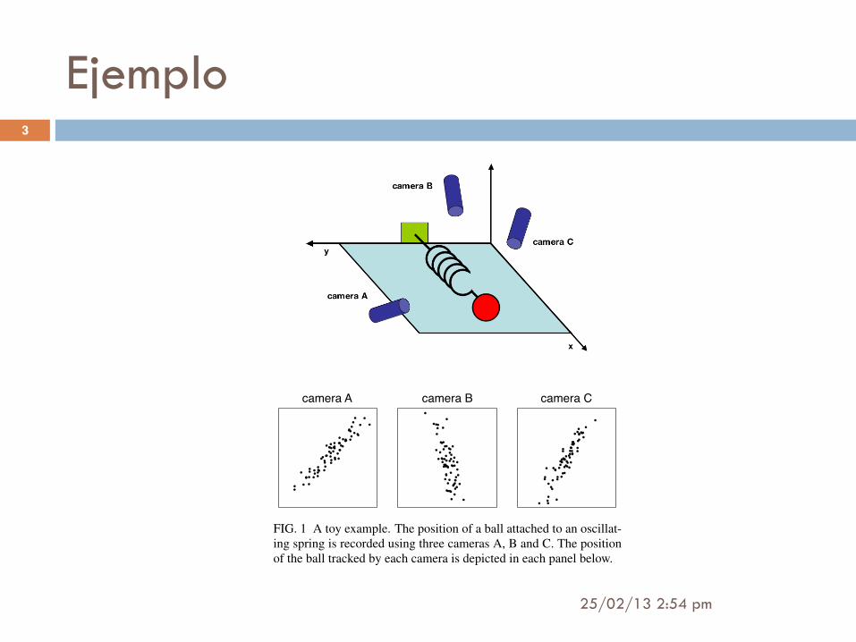
camera A camera B camera C
FIG. 1 A toy example. The position of a ball attached to an oscillat-ing spring is recorded using three cameras A, B and C. The positionof the ball tracked by each camera is depicted in each panel below.
record with the cameras for several minutes. The big questionremains: how do we get from this data set to a simple equation
of x?
We know a-priori that if we were smart experimenters, wewould have just measured the position along the x-axis withone camera. But this is not what happens in the real world.We often do not know which measurements best reflect thedynamics of our system in question. Furthermore, we some-times record more dimensions than we actually need.
Also, we have to deal with that pesky, real-world problem ofnoise. In the toy example this means that we need to dealwith air, imperfect cameras or even friction in a less-than-idealspring. Noise contaminates our data set only serving to obfus-cate the dynamics further. This toy example is the challenge
experimenters face everyday. Keep this example in mind aswe delve further into abstract concepts. Hopefully, by the endof this paper we will have a good understanding of how tosystematically extract x using principal component analysis.
III. FRAMEWORK: CHANGE OF BASIS
The goal of principal component analysis is to identify themost meaningful basis to re-express a data set. The hope isthat this new basis will filter out the noise and reveal hiddenstructure. In the example of the spring, the explicit goal ofPCA is to determine: “the dynamics are along the x-axis.” Inother words, the goal of PCA is to determine that x, i.e. theunit basis vector along the x-axis, is the important dimension.
Determining this fact allows an experimenter to discern whichdynamics are important, redundant or noise.
A. A Naive Basis
With a more precise definition of our goal, we need a moreprecise definition of our data as well. We treat every timesample (or experimental trial) as an individual sample in ourdata set. At each time sample we record a set of data consist-ing of multiple measurements (e.g. voltage, position, etc.). Inour data set, at one point in time, camera A records a corre-sponding ball position (x
A
,yA
). One sample or trial can thenbe expressed as a 6 dimensional column vector
~X =
2
666664
x
A
y
A
x
B
y
B
x
C
y
C
3
777775
where each camera contributes a 2-dimensional projection ofthe ball’s position to the entire vector ~
X . If we record the ball’sposition for 10 minutes at 120 Hz, then we have recorded 10⇥60⇥120 = 72000 of these vectors.
With this concrete example, let us recast this problem in ab-stract terms. Each sample ~
X is an m-dimensional vector,where m is the number of measurement types. Equivalently,every sample is a vector that lies in an m-dimensional vec-tor space spanned by some orthonormal basis. From linearalgebra we know that all measurement vectors form a linearcombination of this set of unit length basis vectors. What isthis orthonormal basis?
This question is usually a tacit assumption often overlooked.Pretend we gathered our toy example data above, but onlylooked at camera A. What is an orthonormal basis for (x
A
,yA
)?A naive choice would be {(1,0),(0,1)}, but why select thisbasis over {(
p2
2 ,p
22 ),(�
p2
2 , �p
22 )} or any other arbitrary rota-
tion? The reason is that the naive basis reflects the method we
gathered the data. Pretend we record the position (2,2). Wedid not record 2
p2 in the (
p2
2 ,p
22 ) direction and 0 in the per-
pendicular direction. Rather, we recorded the position (2,2)on our camera meaning 2 units up and 2 units to the left in ourcamera window. Thus our original basis reflects the methodwe measured our data.
How do we express this naive basis in linear algebra? In thetwo dimensional case, {(1,0),(0,1)} can be recast as individ-ual row vectors. A matrix constructed out of these row vectorsis the 2⇥2 identity matrix I. We can generalize this to the m-dimensional case by constructing an m⇥m identity matrix
B =
2
664
b
1
b
2
...b
m
3
775 =
2
664
1 0 · · · 00 1 · · · 0...
.... . .
...0 0 · · · 1
3
775 = I
3

PCA
25/02/13 2:54 pm
¨ ¿Cómo representamos el conjunto de datos con una ecuación simple?
¨ Ademas, tenemos que trabajar con datos con ruido
4

Cambio de Bases
25/02/13 2:54 pm
¨ Meta en PCA ¤ Identificar las bases más significativas para re-
expresar el conjunto de datos ¤ Esperamos que la nueva base
n Filtre el ruido n Revele la estructura oculta
5

Base Naive
25/02/13 2:54 pm
¨ Representamos cada muestra de nuestro conjunto de datos ¤ Las coordenadas observadas en cada cámara
n Obtenemos la posición de la bola por 10 minutos a 120 Hz. n 10 x 60 x 120 = 72,000 muestras (vectores)
n X es un espacio vectoral m-dimensional generado por una base ortonormal
6
2
camera A camera B camera C
FIG. 1 A toy example. The position of a ball attached to an oscillat-ing spring is recorded using three cameras A, B and C. The positionof the ball tracked by each camera is depicted in each panel below.
record with the cameras for several minutes. The big questionremains: how do we get from this data set to a simple equation
of x?
We know a-priori that if we were smart experimenters, wewould have just measured the position along the x-axis withone camera. But this is not what happens in the real world.We often do not know which measurements best reflect thedynamics of our system in question. Furthermore, we some-times record more dimensions than we actually need.
Also, we have to deal with that pesky, real-world problem ofnoise. In the toy example this means that we need to dealwith air, imperfect cameras or even friction in a less-than-idealspring. Noise contaminates our data set only serving to obfus-cate the dynamics further. This toy example is the challenge
experimenters face everyday. Keep this example in mind aswe delve further into abstract concepts. Hopefully, by the endof this paper we will have a good understanding of how tosystematically extract x using principal component analysis.
III. FRAMEWORK: CHANGE OF BASIS
The goal of principal component analysis is to identify themost meaningful basis to re-express a data set. The hope isthat this new basis will filter out the noise and reveal hiddenstructure. In the example of the spring, the explicit goal ofPCA is to determine: “the dynamics are along the x-axis.” Inother words, the goal of PCA is to determine that x, i.e. theunit basis vector along the x-axis, is the important dimension.
Determining this fact allows an experimenter to discern whichdynamics are important, redundant or noise.
A. A Naive Basis
With a more precise definition of our goal, we need a moreprecise definition of our data as well. We treat every timesample (or experimental trial) as an individual sample in ourdata set. At each time sample we record a set of data consist-ing of multiple measurements (e.g. voltage, position, etc.). Inour data set, at one point in time, camera A records a corre-sponding ball position (x
A
,yA
). One sample or trial can thenbe expressed as a 6 dimensional column vector
~X =
2
666664
x
A
y
A
x
B
y
B
x
C
y
C
3
777775
where each camera contributes a 2-dimensional projection ofthe ball’s position to the entire vector ~
X . If we record the ball’sposition for 10 minutes at 120 Hz, then we have recorded 10⇥60⇥120 = 72000 of these vectors.
With this concrete example, let us recast this problem in ab-stract terms. Each sample ~
X is an m-dimensional vector,where m is the number of measurement types. Equivalently,every sample is a vector that lies in an m-dimensional vec-tor space spanned by some orthonormal basis. From linearalgebra we know that all measurement vectors form a linearcombination of this set of unit length basis vectors. What isthis orthonormal basis?
This question is usually a tacit assumption often overlooked.Pretend we gathered our toy example data above, but onlylooked at camera A. What is an orthonormal basis for (x
A
,yA
)?A naive choice would be {(1,0),(0,1)}, but why select thisbasis over {(
p2
2 ,p
22 ),(�
p2
2 , �p
22 )} or any other arbitrary rota-
tion? The reason is that the naive basis reflects the method we
gathered the data. Pretend we record the position (2,2). Wedid not record 2
p2 in the (
p2
2 ,p
22 ) direction and 0 in the per-
pendicular direction. Rather, we recorded the position (2,2)on our camera meaning 2 units up and 2 units to the left in ourcamera window. Thus our original basis reflects the methodwe measured our data.
How do we express this naive basis in linear algebra? In thetwo dimensional case, {(1,0),(0,1)} can be recast as individ-ual row vectors. A matrix constructed out of these row vectorsis the 2⇥2 identity matrix I. We can generalize this to the m-dimensional case by constructing an m⇥m identity matrix
B =
2
664
b
1
b
2
...b
m
3
775 =
2
664
1 0 · · · 00 1 · · · 0...
.... . .
...0 0 · · · 1
3
775 = I

Base Naive
25/02/13 2:54 pm
¨ Si vemos solo la cámara A ¤ ¿Cuál es una base ortonormal para (XA, YA)? ¤ Una elección naive sería {(1,0), (0,1)}
n Refleja el método con el que se obtuvieron los datos
¤ Hay otras opciones {(sqrt(2)/2) (sqrt(2)/2), (-sqrt(2)/2) (-sqrt(2)/2)} u otra rotación
7

Base Naive
25/02/13 2:54 pm
¨ ¿Cómo representamos la base naive en álgebra lineal? ¤ Cada renglón es un vector base ortonormal bi con m
componentes
8
2
camera A camera B camera C
FIG. 1 A toy example. The position of a ball attached to an oscillat-ing spring is recorded using three cameras A, B and C. The positionof the ball tracked by each camera is depicted in each panel below.
record with the cameras for several minutes. The big questionremains: how do we get from this data set to a simple equation
of x?
We know a-priori that if we were smart experimenters, wewould have just measured the position along the x-axis withone camera. But this is not what happens in the real world.We often do not know which measurements best reflect thedynamics of our system in question. Furthermore, we some-times record more dimensions than we actually need.
Also, we have to deal with that pesky, real-world problem ofnoise. In the toy example this means that we need to dealwith air, imperfect cameras or even friction in a less-than-idealspring. Noise contaminates our data set only serving to obfus-cate the dynamics further. This toy example is the challenge
experimenters face everyday. Keep this example in mind aswe delve further into abstract concepts. Hopefully, by the endof this paper we will have a good understanding of how tosystematically extract x using principal component analysis.
III. FRAMEWORK: CHANGE OF BASIS
The goal of principal component analysis is to identify themost meaningful basis to re-express a data set. The hope isthat this new basis will filter out the noise and reveal hiddenstructure. In the example of the spring, the explicit goal ofPCA is to determine: “the dynamics are along the x-axis.” Inother words, the goal of PCA is to determine that x, i.e. theunit basis vector along the x-axis, is the important dimension.
Determining this fact allows an experimenter to discern whichdynamics are important, redundant or noise.
A. A Naive Basis
With a more precise definition of our goal, we need a moreprecise definition of our data as well. We treat every timesample (or experimental trial) as an individual sample in ourdata set. At each time sample we record a set of data consist-ing of multiple measurements (e.g. voltage, position, etc.). Inour data set, at one point in time, camera A records a corre-sponding ball position (x
A
,yA
). One sample or trial can thenbe expressed as a 6 dimensional column vector
~X =
2
666664
x
A
y
A
x
B
y
B
x
C
y
C
3
777775
where each camera contributes a 2-dimensional projection ofthe ball’s position to the entire vector ~
X . If we record the ball’sposition for 10 minutes at 120 Hz, then we have recorded 10⇥60⇥120 = 72000 of these vectors.
With this concrete example, let us recast this problem in ab-stract terms. Each sample ~
X is an m-dimensional vector,where m is the number of measurement types. Equivalently,every sample is a vector that lies in an m-dimensional vec-tor space spanned by some orthonormal basis. From linearalgebra we know that all measurement vectors form a linearcombination of this set of unit length basis vectors. What isthis orthonormal basis?
This question is usually a tacit assumption often overlooked.Pretend we gathered our toy example data above, but onlylooked at camera A. What is an orthonormal basis for (x
A
,yA
)?A naive choice would be {(1,0),(0,1)}, but why select thisbasis over {(
p2
2 ,p
22 ),(�
p2
2 , �p
22 )} or any other arbitrary rota-
tion? The reason is that the naive basis reflects the method we
gathered the data. Pretend we record the position (2,2). Wedid not record 2
p2 in the (
p2
2 ,p
22 ) direction and 0 in the per-
pendicular direction. Rather, we recorded the position (2,2)on our camera meaning 2 units up and 2 units to the left in ourcamera window. Thus our original basis reflects the methodwe measured our data.
How do we express this naive basis in linear algebra? In thetwo dimensional case, {(1,0),(0,1)} can be recast as individ-ual row vectors. A matrix constructed out of these row vectorsis the 2⇥2 identity matrix I. We can generalize this to the m-dimensional case by constructing an m⇥m identity matrix
B =
2
664
b
1
b
2
...b
m
3
775 =
2
664
1 0 · · · 00 1 · · · 0...
.... . .
...0 0 · · · 1
3
775 = I

Cambio de Base
25/02/13 2:54 pm
¨ Pregunta de PCA ¤ ¿Hay otra base, una combinación lineal de las bases
originales, que mejor exprese el conjunto de datos? ¤ Linearidad à simplifica el problema
n Restringe el conjunto de bases potenciales
9

Cambio de Base
25/02/13 2:54 pm
¨ Sea ¤ X, el conjunto de datos original
n Cada columna es una muestra independiente n En el ejemplo, X es una matrix de m x n
n m = 6 n n = 72,000
¤ Y, otra matriz de m x n, relacionada por una transformación lineal P n Y es una nueva representación de los datos originales
10
3
where each row is an orthornormal basis vector b
i
with m
components. We can consider our naive basis as the effectivestarting point. All of our data has been recorded in this basisand thus it can be trivially expressed as a linear combinationof {b
i
}.
B. Change of Basis
With this rigor we may now state more precisely what PCAasks: Is there another basis, which is a linear combination of
the original basis, that best re-expresses our data set?
A close reader might have noticed the conspicuous addition ofthe word linear. Indeed, PCA makes one stringent but power-ful assumption: linearity. Linearity vastly simplifies the prob-lem by restricting the set of potential bases. With this assump-tion PCA is now limited to re-expressing the data as a linear
combination of its basis vectors.
Let X be the original data set, where each column is a singlesample (or moment in time) of our data set (i.e. ~
X). In the toyexample X is an m⇥ n matrix where m = 6 and n = 72000.Let Y be another m⇥ n matrix related by a linear transfor-mation P. X is the original recorded data set and Y is a newrepresentation of that data set.
PX = Y (1)
Also let us define the following quantities.1
• p
i
are the rows of P
• x
i
are the columns of X (or individual ~X).
• y
i
are the columns of Y.
Equation 1 represents a change of basis and thus can havemany interpretations.
1. P is a matrix that transforms X into Y.
2. Geometrically, P is a rotation and a stretch which againtransforms X into Y.
3. The rows of P, {p
1
, . . . ,pm
}, are a set of new basis vec-tors for expressing the columns of X.
The latter interpretation is not obvious but can be seen by writ-
1 In this section x
i
and y
i
are column vectors, but be forewarned. In all othersections x
i
and y
i
are row vectors.
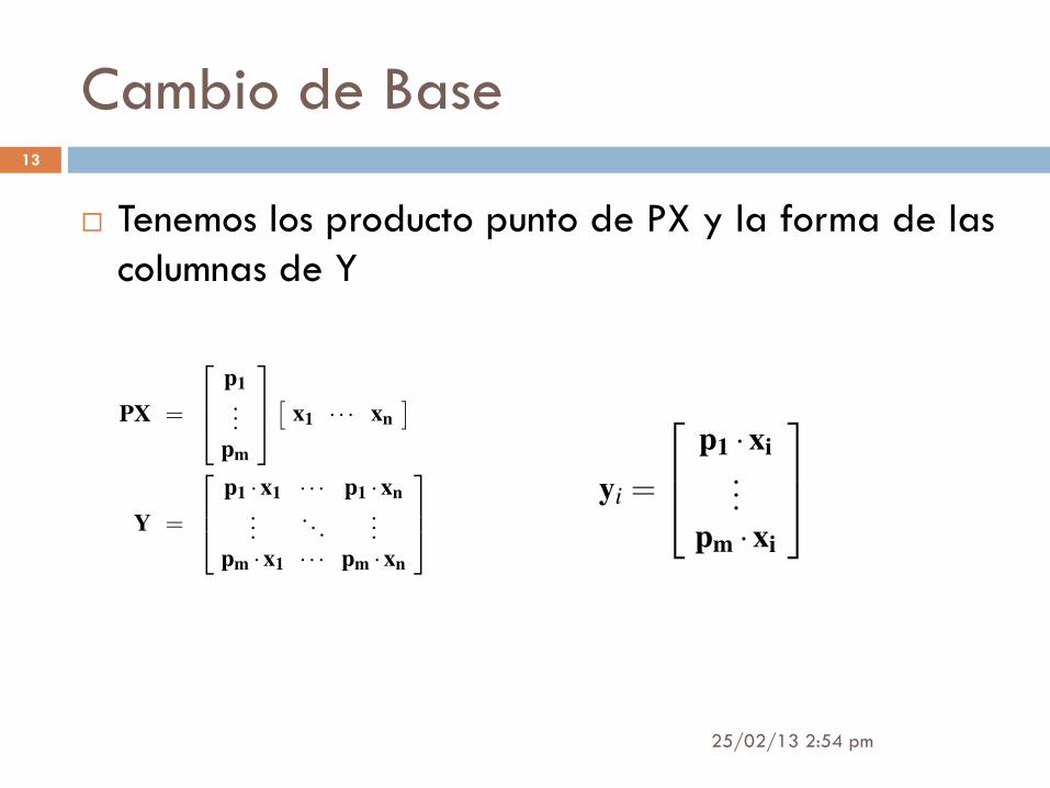
ing out the explicit dot products of PX.
PX =
2
64p
1
...p
m
3
75⇥
x
1
· · · x
n
⇤
Y =
2
64p
1
·x1
· · · p
1
·xn
.... . .
...p
m
·x1
· · · p
m
·xn
3
75
We can note the form of each column of Y.
y
i
=
2
64p
1
·xi
...p
m
·xi
3
75
We recognize that each coefficient of y
i
is a dot-product ofx
i
with the corresponding row in P. In other words, the j
th
coefficient of y
i
is a projection on to the j
th row of P. This isin fact the very form of an equation where y
i
is a projectionon to the basis of {p
1
, . . . ,pm
}. Therefore, the rows of P are anew set of basis vectors for representing of columns of X.
C. Questions Remaining
By assuming linearity the problem reduces to finding the ap-propriate change of basis. The row vectors {p
1
, . . . ,pm
} inthis transformation will become the principal components ofX. Several questions now arise.
• What is the best way to re-express X?
• What is a good choice of basis P?
These questions must be answered by next asking ourselveswhat features we would like Y to exhibit. Evidently, addi-tional assumptions beyond linearity are required to arrive ata reasonable result. The selection of these assumptions is thesubject of the next section.
IV. VARIANCE AND THE GOAL
Now comes the most important question: what does best ex-
press the data mean? This section will build up an intuitiveanswer to this question and along the way tack on additionalassumptions.
A. Noise and Rotation
Measurement noise in any data set must be low or else, nomatter the analysis technique, no information about a signal

Cambio de Base
25/02/13 2:54 pm
¨ Definamos las siguientes cantidades: ¤ pi son los renglones de P ¤ xi son las columnas de X (o muestras individuales) ¤ yi son las columnas de Y
11

Cambio de Base
25/02/13 2:54 pm
¨ La ecuación representa un cambio de base y puede tener muchas interpretaciones ¤ P es una matriz que transforma X en Y ¤ Geométricamente, P es una rotación y estiración, la
cual transforma X en Y ¤ Los renglones de P {p1, …, pm} son un nuevo conjunto
de vectores base para expresar las columnas de X
12
Cambio de Base
25/02/13 2:54 pm
13
¨ Tenemos los producto punto de PX y la forma de las columnas de Y 3
where each row is an orthornormal basis vector b
i
with m
components. We can consider our naive basis as the effectivestarting point. All of our data has been recorded in this basisand thus it can be trivially expressed as a linear combinationof {b
i
}.
B. Change of Basis
With this rigor we may now state more precisely what PCAasks: Is there another basis, which is a linear combination of
the original basis, that best re-expresses our data set?
A close reader might have noticed the conspicuous addition ofthe word linear. Indeed, PCA makes one stringent but power-ful assumption: linearity. Linearity vastly simplifies the prob-lem by restricting the set of potential bases. With this assump-tion PCA is now limited to re-expressing the data as a linear
combination of its basis vectors.
Let X be the original data set, where each column is a singlesample (or moment in time) of our data set (i.e. ~
X). In the toyexample X is an m⇥ n matrix where m = 6 and n = 72000.Let Y be another m⇥ n matrix related by a linear transfor-mation P. X is the original recorded data set and Y is a newrepresentation of that data set.
PX = Y (1)
Also let us define the following quantities.1
• p
i
are the rows of P
• x
i
are the columns of X (or individual ~X).
• y
i
are the columns of Y.
Equation 1 represents a change of basis and thus can havemany interpretations.
1. P is a matrix that transforms X into Y.
2. Geometrically, P is a rotation and a stretch which againtransforms X into Y.
3. The rows of P, {p
1
, . . . ,pm
}, are a set of new basis vec-tors for expressing the columns of X.
The latter interpretation is not obvious but can be seen by writ-
1 In this section x
i
and y
i
are column vectors, but be forewarned. In all othersections x
i
and y
i
are row vectors.
ing out the explicit dot products of PX.
PX =
2
64p
1
...p
m
3
75⇥
x
1
· · · x
n
⇤
Y =
2
64p
1
·x1
· · · p
1
·xn
.... . .
...p
m
·x1
· · · p
m
·xn
3
75
We can note the form of each column of Y.
y
i
=
2
64p
1
·xi
...p
m
·xi
3
75
We recognize that each coefficient of y
i
is a dot-product ofx
i
with the corresponding row in P. In other words, the j
th
coefficient of y
i
is a projection on to the j
th row of P. This isin fact the very form of an equation where y
i
is a projectionon to the basis of {p
1
, . . . ,pm
}. Therefore, the rows of P are anew set of basis vectors for representing of columns of X.
C. Questions Remaining
By assuming linearity the problem reduces to finding the ap-propriate change of basis. The row vectors {p
1
, . . . ,pm
} inthis transformation will become the principal components ofX. Several questions now arise.
• What is the best way to re-express X?
• What is a good choice of basis P?
These questions must be answered by next asking ourselveswhat features we would like Y to exhibit. Evidently, addi-tional assumptions beyond linearity are required to arrive ata reasonable result. The selection of these assumptions is thesubject of the next section.
IV. VARIANCE AND THE GOAL
Now comes the most important question: what does best ex-
press the data mean? This section will build up an intuitiveanswer to this question and along the way tack on additionalassumptions.
A. Noise and Rotation
Measurement noise in any data set must be low or else, nomatter the analysis technique, no information about a signal
3
where each row is an orthornormal basis vector b
i
with m
components. We can consider our naive basis as the effectivestarting point. All of our data has been recorded in this basisand thus it can be trivially expressed as a linear combinationof {b
i
}.
B. Change of Basis
With this rigor we may now state more precisely what PCAasks: Is there another basis, which is a linear combination of
the original basis, that best re-expresses our data set?
A close reader might have noticed the conspicuous addition ofthe word linear. Indeed, PCA makes one stringent but power-ful assumption: linearity. Linearity vastly simplifies the prob-lem by restricting the set of potential bases. With this assump-tion PCA is now limited to re-expressing the data as a linear
combination of its basis vectors.
Let X be the original data set, where each column is a singlesample (or moment in time) of our data set (i.e. ~
X). In the toyexample X is an m⇥ n matrix where m = 6 and n = 72000.Let Y be another m⇥ n matrix related by a linear transfor-mation P. X is the original recorded data set and Y is a newrepresentation of that data set.
PX = Y (1)
Also let us define the following quantities.1
• p
i
are the rows of P
• x
i
are the columns of X (or individual ~X).
• y
i
are the columns of Y.
Equation 1 represents a change of basis and thus can havemany interpretations.
1. P is a matrix that transforms X into Y.
2. Geometrically, P is a rotation and a stretch which againtransforms X into Y.
3. The rows of P, {p
1
, . . . ,pm
}, are a set of new basis vec-tors for expressing the columns of X.
The latter interpretation is not obvious but can be seen by writ-
1 In this section x
i
and y
i
are column vectors, but be forewarned. In all othersections x
i
and y
i
are row vectors.
ing out the explicit dot products of PX.
PX =
2
64p
1
...p
m
3
75⇥
x
1
· · · x
n
⇤
Y =
2
64p
1
·x1
· · · p
1
·xn
.... . .
...p
m
·x1
· · · p
m
·xn
3
75
We can note the form of each column of Y.
y
i
=
2
64p
1
·xi
...p
m
·xi
3
75
We recognize that each coefficient of y
i
is a dot-product ofx
i
with the corresponding row in P. In other words, the j
th
coefficient of y
i
is a projection on to the j
th row of P. This isin fact the very form of an equation where y
i
is a projectionon to the basis of {p
1
, . . . ,pm
}. Therefore, the rows of P are anew set of basis vectors for representing of columns of X.
C. Questions Remaining
By assuming linearity the problem reduces to finding the ap-propriate change of basis. The row vectors {p
1
, . . . ,pm
} inthis transformation will become the principal components ofX. Several questions now arise.
• What is the best way to re-express X?
• What is a good choice of basis P?
These questions must be answered by next asking ourselveswhat features we would like Y to exhibit. Evidently, addi-tional assumptions beyond linearity are required to arrive ata reasonable result. The selection of these assumptions is thesubject of the next section.
IV. VARIANCE AND THE GOAL
Now comes the most important question: what does best ex-
press the data mean? This section will build up an intuitiveanswer to this question and along the way tack on additionalassumptions.
A. Noise and Rotation
Measurement noise in any data set must be low or else, nomatter the analysis technique, no information about a signal

Preguntas Restantes
25/02/13 2:54 pm
¨ Los vectores renglón {p1, .., pm} en esta transformación serán los componentes principales de X ¤ ¿Cuál es la mejor manera de re-expresar X? ¤ ¿Cuál es una buena elección de base P?
¨ Estas preguntas se responden al preguntarnos ¤ ¿Qué carácterísticas nos gustaría que tuviera Y?
14

Varianza y la Meta
25/02/13 2:54 pm
¨ La pregunta más importante ¨ ¿Qué expresa la media de los datos lo mejor posible?
15

Ruido y Rotación
25/02/13 2:54 pm
¨ No existe una escala absoluta para el ruido ¨ Sin embargo, se puede cuantificar relativo a la
fuerza de la señal ¤ Medida común: signal-to-noise ratio (SNR), o un radio
de varianzas σ2
n SNR (>>1) indica una medición altamente precisa n SNR baja, indica datos con mucho ruido
16
4
σ 2signal
σ 2noise
x
y
FIG. 2 Simulated data of (x,y) for camera A. The signal and noisevariances s2
signal
and s2noise
are graphically represented by the twolines subtending the cloud of data. Note that the largest directionof variance does not lie along the basis of the recording (x
A
,yA
) butrather along the best-fit line.
can be extracted. There exists no absolute scale for noise butrather all noise is quantified relative to the signal strength. Acommon measure is the signal-to-noise ratio (SNR), or a ratioof variances s2,
SNR =s2
signal
s2noise
.
A high SNR (� 1) indicates a high precision measurement,while a low SNR indicates very noisy data.
Let’s take a closer examination of the data from cameraA in Figure 2. Remembering that the spring travels in astraight line, every individual camera should record motion ina straight line as well. Therefore, any spread deviating fromstraight-line motion is noise. The variance due to the signaland noise are indicated by each line in the diagram. The ratioof the two lengths measures how skinny the cloud is: possibil-ities include a thin line (SNR� 1), a circle (SNR = 1) or evenworse. By positing reasonably good measurements, quantita-tively we assume that directions with largest variances in ourmeasurement space contain the dynamics of interest. In Fig-ure 2 the direction with the largest variance is not x
A
= (1,0)nor y
A
= (0,1), but the direction along the long axis of thecloud. Thus, by assumption the dynamics of interest existalong directions with largest variance and presumably high-est SNR.
Our assumption suggests that the basis for which we aresearching is not the naive basis because these directions (i.e.(x
A
,yA
)) do not correspond to the directions of largest vari-ance. Maximizing the variance (and by assumption the SNR)corresponds to finding the appropriate rotation of the naivebasis. This intuition corresponds to finding the direction indi-cated by the line s2
signal
in Figure 2. In the 2-dimensional caseof Figure 2 the direction of largest variance corresponds to thebest-fit line for the data cloud. Thus, rotating the naive basisto lie parallel to the best-fit line would reveal the direction ofmotion of the spring for the 2-D case. How do we generalizethis notion to an arbitrary number of dimensions? Before weapproach this question we need to examine this issue from asecond perspective.
low redundancy high redundancy
r1
r2
r1
r2
r1
r2
FIG. 3 A spectrum of possible redundancies in data from the twoseparate measurements r1 and r2. The two measurements on theleft are uncorrelated because one can not predict one from the other.Conversely, the two measurements on the right are highly correlatedindicating highly redundant measurements.
B. Redundancy
Figure 2 hints at an additional confounding factor in our data- redundancy. This issue is particularly evident in the exampleof the spring. In this case multiple sensors record the samedynamic information. Reexamine Figure 2 and ask whetherit was really necessary to record 2 variables. Figure 3 mightreflect a range of possibile plots between two arbitrary mea-surement types r1 and r2. The left-hand panel depicts tworecordings with no apparent relationship. Because one can notpredict r1 from r2, one says that r1 and r2 are uncorrelated.
On the other extreme, the right-hand panel of Figure 3 de-picts highly correlated recordings. This extremity might beachieved by several means:
• A plot of (xA
,xB
) if cameras A and B are very nearby.
• A plot of (xA
, xA
) where x
A
is in meters and x
A
is ininches.
Clearly in the right panel of Figure 3 it would be more mean-ingful to just have recorded a single variable, not both. Why?Because one can calculate r1 from r2 (or vice versa) using thebest-fit line. Recording solely one response would express thedata more concisely and reduce the number of sensor record-ings (2! 1 variables). Indeed, this is the central idea behinddimensional reduction.
C. Covariance Matrix
In a 2 variable case it is simple to identify redundant cases byfinding the slope of the best-fit line and judging the quality ofthe fit. How do we quantify and generalize these notions toarbitrarily higher dimensions? Consider two sets of measure-ments with zero means
A = {a1,a2, . . . ,an
} , B = {b1,b2, . . . ,bn
}

Ruido y Rotación
25/02/13 2:54 pm
17
¨ En el ejemplo ¤ Cualquier desviación de la línea recta del movimiento
de la pelota es ruido
¨ Si consideramos razonablemente buenas mediciones ¤ Podemos asumir (cuantitativamente)
n Las direcciones con las varianzas más altas en nuestro espacio de mediciones contiene la dinámica de interés
¨ La dirección con la varianza más alta no es X^ = (1, 0), ni Y^ = (0, 1); sino la dirección a lo largo del eje de la nube.

Ruido y Rotación
25/02/13 2:54 pm
4
σ 2signal
σ 2noise
x
y
FIG. 2 Simulated data of (x,y) for camera A. The signal and noisevariances s2
signal
and s2noise
are graphically represented by the twolines subtending the cloud of data. Note that the largest directionof variance does not lie along the basis of the recording (x
A
,yA
) butrather along the best-fit line.
can be extracted. There exists no absolute scale for noise butrather all noise is quantified relative to the signal strength. Acommon measure is the signal-to-noise ratio (SNR), or a ratioof variances s2,
SNR =s2
signal
s2noise
.
A high SNR (� 1) indicates a high precision measurement,while a low SNR indicates very noisy data.
Let’s take a closer examination of the data from cameraA in Figure 2. Remembering that the spring travels in astraight line, every individual camera should record motion ina straight line as well. Therefore, any spread deviating fromstraight-line motion is noise. The variance due to the signaland noise are indicated by each line in the diagram. The ratioof the two lengths measures how skinny the cloud is: possibil-ities include a thin line (SNR� 1), a circle (SNR = 1) or evenworse. By positing reasonably good measurements, quantita-tively we assume that directions with largest variances in ourmeasurement space contain the dynamics of interest. In Fig-ure 2 the direction with the largest variance is not x
A
= (1,0)nor y
A
= (0,1), but the direction along the long axis of thecloud. Thus, by assumption the dynamics of interest existalong directions with largest variance and presumably high-est SNR.
Our assumption suggests that the basis for which we aresearching is not the naive basis because these directions (i.e.(x
A
,yA
)) do not correspond to the directions of largest vari-ance. Maximizing the variance (and by assumption the SNR)corresponds to finding the appropriate rotation of the naivebasis. This intuition corresponds to finding the direction indi-cated by the line s2
signal
in Figure 2. In the 2-dimensional caseof Figure 2 the direction of largest variance corresponds to thebest-fit line for the data cloud. Thus, rotating the naive basisto lie parallel to the best-fit line would reveal the direction ofmotion of the spring for the 2-D case. How do we generalizethis notion to an arbitrary number of dimensions? Before weapproach this question we need to examine this issue from asecond perspective.
low redundancy high redundancy
r1
r2
r1
r2
r1
r2
FIG. 3 A spectrum of possible redundancies in data from the twoseparate measurements r1 and r2. The two measurements on theleft are uncorrelated because one can not predict one from the other.Conversely, the two measurements on the right are highly correlatedindicating highly redundant measurements.
B. Redundancy
Figure 2 hints at an additional confounding factor in our data- redundancy. This issue is particularly evident in the exampleof the spring. In this case multiple sensors record the samedynamic information. Reexamine Figure 2 and ask whetherit was really necessary to record 2 variables. Figure 3 mightreflect a range of possibile plots between two arbitrary mea-surement types r1 and r2. The left-hand panel depicts tworecordings with no apparent relationship. Because one can notpredict r1 from r2, one says that r1 and r2 are uncorrelated.
On the other extreme, the right-hand panel of Figure 3 de-picts highly correlated recordings. This extremity might beachieved by several means:
• A plot of (xA
,xB
) if cameras A and B are very nearby.
• A plot of (xA
, xA
) where x
A
is in meters and x
A
is ininches.
Clearly in the right panel of Figure 3 it would be more mean-ingful to just have recorded a single variable, not both. Why?Because one can calculate r1 from r2 (or vice versa) using thebest-fit line. Recording solely one response would express thedata more concisely and reduce the number of sensor record-ings (2! 1 variables). Indeed, this is the central idea behinddimensional reduction.
C. Covariance Matrix
In a 2 variable case it is simple to identify redundant cases byfinding the slope of the best-fit line and judging the quality ofthe fit. How do we quantify and generalize these notions toarbitrarily higher dimensions? Consider two sets of measure-ments with zero means
A = {a1,a2, . . . ,an
} , B = {b1,b2, . . . ,bn
}
18
Ruido y Rotación
25/02/13 2:54 pm
¨ Maximizar la varianza y por asunción la SNR ¨ Corresponde a encontrar la rotación apropiada de la base
naive ¨ Encontrar la dirección indicada por la línea σ2
SIGNAL de la figura
¨ En 2 dimensiones, la dirección de mayor varianza corresponde a la línea de mejor ajuste para la nube de datos ¨ Rotamos la base naive para que sea paralela a la línea de
mejor ajuste ¨ Revelará la dirección del movimiento del resorte y la pelota
19

Redundancia
25/02/13 2:54 pm
¨ Un factor más para confundirnos en el análisis es la redundancia
¨ En el ejemplo tenemos redundancia porque ¤ Múltiples sensores graban la información de la misma
dinámica ¤ ¿Era necesario grabar dos variables?
n Medidas altamente correlacionadas n Si las cámaras A y B están muy cerca n Si una medida se toma en metros y la otra en pulgadas
n En algunos casos una sola medida es suficiente n Podemos calcular r1 a partir de r2
20

Redundancia
25/02/13 2:54 pm
4
σ 2signal
σ 2noise
x
y
FIG. 2 Simulated data of (x,y) for camera A. The signal and noisevariances s2
signal
and s2noise
are graphically represented by the twolines subtending the cloud of data. Note that the largest directionof variance does not lie along the basis of the recording (x
A
,yA
) butrather along the best-fit line.
can be extracted. There exists no absolute scale for noise butrather all noise is quantified relative to the signal strength. Acommon measure is the signal-to-noise ratio (SNR), or a ratioof variances s2,
SNR =s2
signal
s2noise
.
A high SNR (� 1) indicates a high precision measurement,while a low SNR indicates very noisy data.
Let’s take a closer examination of the data from cameraA in Figure 2. Remembering that the spring travels in astraight line, every individual camera should record motion ina straight line as well. Therefore, any spread deviating fromstraight-line motion is noise. The variance due to the signaland noise are indicated by each line in the diagram. The ratioof the two lengths measures how skinny the cloud is: possibil-ities include a thin line (SNR� 1), a circle (SNR = 1) or evenworse. By positing reasonably good measurements, quantita-tively we assume that directions with largest variances in ourmeasurement space contain the dynamics of interest. In Fig-ure 2 the direction with the largest variance is not x
A
= (1,0)nor y
A
= (0,1), but the direction along the long axis of thecloud. Thus, by assumption the dynamics of interest existalong directions with largest variance and presumably high-est SNR.
Our assumption suggests that the basis for which we aresearching is not the naive basis because these directions (i.e.(x
A
,yA
)) do not correspond to the directions of largest vari-ance. Maximizing the variance (and by assumption the SNR)corresponds to finding the appropriate rotation of the naivebasis. This intuition corresponds to finding the direction indi-cated by the line s2
signal
in Figure 2. In the 2-dimensional caseof Figure 2 the direction of largest variance corresponds to thebest-fit line for the data cloud. Thus, rotating the naive basisto lie parallel to the best-fit line would reveal the direction ofmotion of the spring for the 2-D case. How do we generalizethis notion to an arbitrary number of dimensions? Before weapproach this question we need to examine this issue from asecond perspective.
low redundancy high redundancy
r1
r2
r1
r2
r1
r2
FIG. 3 A spectrum of possible redundancies in data from the twoseparate measurements r1 and r2. The two measurements on theleft are uncorrelated because one can not predict one from the other.Conversely, the two measurements on the right are highly correlatedindicating highly redundant measurements.
B. Redundancy
Figure 2 hints at an additional confounding factor in our data- redundancy. This issue is particularly evident in the exampleof the spring. In this case multiple sensors record the samedynamic information. Reexamine Figure 2 and ask whetherit was really necessary to record 2 variables. Figure 3 mightreflect a range of possibile plots between two arbitrary mea-surement types r1 and r2. The left-hand panel depicts tworecordings with no apparent relationship. Because one can notpredict r1 from r2, one says that r1 and r2 are uncorrelated.
On the other extreme, the right-hand panel of Figure 3 de-picts highly correlated recordings. This extremity might beachieved by several means:
• A plot of (xA
,xB
) if cameras A and B are very nearby.
• A plot of (xA
, xA
) where x
A
is in meters and x
A
is ininches.
Clearly in the right panel of Figure 3 it would be more mean-ingful to just have recorded a single variable, not both. Why?Because one can calculate r1 from r2 (or vice versa) using thebest-fit line. Recording solely one response would express thedata more concisely and reduce the number of sensor record-ings (2! 1 variables). Indeed, this is the central idea behinddimensional reduction.
C. Covariance Matrix
In a 2 variable case it is simple to identify redundant cases byfinding the slope of the best-fit line and judging the quality ofthe fit. How do we quantify and generalize these notions toarbitrarily higher dimensions? Consider two sets of measure-ments with zero means
A = {a1,a2, . . . ,an
} , B = {b1,b2, . . . ,bn
}
21

Matriz de Covarianza
25/02/13 2:54 pm
¨ En 2 dimensiones es fácil identificar casos redundantes ¤ Encontrar la pendiente con mejor ajuste y verificando la
calidad del ajuste
¨ ¿Cómo cuantificamos y generalizamos estas nociones a dimensiones más altas? ¤ Conjuntos de medidas con media cero
n A = {a1, a2, …, an}, B = {b1, b2, …, bn} n El sub-script denota el número de muestra
22

Matriz de Covarianza
25/02/13 2:54 pm
¨ Varianzas individuales de A y B
¨ Covarianza entre A y B
¨ La covarianza entre 2 variables mide el grado de la relación lineal entre ellas
23
5
where the subscript denotes the sample number. The varianceof A and B are individually defined as,
s2A
=1n
Âi
a
2i
, s2B
=1n
Âi
b
2i
The covariance between A and B is a straight-forward gener-alization.
covariance o f A and B⌘ s2AB
=1n
Âi
a
i
b
i
The covariance measures the degree of the linear relationshipbetween two variables. A large positive value indicates pos-itively correlated data. Likewise, a large negative value de-notes negatively correlated data. The absolute magnitude ofthe covariance measures the degree of redundancy. Some ad-ditional facts about the covariance.
• sAB
is zero if and only if A and B are uncorrelated (e.g.Figure 2, left panel).
• s2AB
= s2A
if A = B.
We can equivalently convert A and B into corresponding rowvectors.
a = [a1 a2 . . . a
n
]b = [b1 b2 . . . b
n
]
so that we may express the covariance as a dot product matrixcomputation.2
s2ab
⌘ 1n
ab
T (2)
Finally, we can generalize from two vectors to an arbitrarynumber. Rename the row vectors a and b as x
1
and x
2
, respec-tively, and consider additional indexed row vectors x
3
, . . . ,xm
.Define a new m⇥n matrix X.
X =
2
64x
1
...x
m
3
75
One interpretation of X is the following. Each row of X corre-sponds to all measurements of a particular type. Each column
of X corresponds to a set of measurements from one particulartrial (this is ~
X from section 3.1). We now arrive at a definitionfor the covariance matrix C
X
.
C
X
⌘ 1n
XX
T .
2 Note that in practice, the covariance s2AB
is calculated as 1n�1 Â
i
a
i
b
i
. Theslight change in normalization constant arises from estimation theory, butthat is beyond the scope of this tutorial.
Consider the matrix C
X
= 1n
XX
T . The i j
th element of C
X
is the dot product between the vector of the i
th measurementtype with the vector of the j
th measurement type. We cansummarize several properties of C
X
:
• C
X
is a square symmetric m⇥m matrix (Theorem 2 ofAppendix A)
• The diagonal terms of C
X
are the variance of particularmeasurement types.
• The off-diagonal terms of C
X
are the covariance be-tween measurement types.
C
X
captures the covariance between all possible pairs of mea-surements. The covariance values reflect the noise and redun-dancy in our measurements.
• In the diagonal terms, by assumption, large values cor-respond to interesting structure.
• In the off-diagonal terms large magnitudes correspondto high redundancy.
Pretend we have the option of manipulating C
X
. We will sug-gestively define our manipulated covariance matrix C
Y
. Whatfeatures do we want to optimize in C
Y
?
D. Diagonalize the Covariance Matrix
We can summarize the last two sections by stating that ourgoals are (1) to minimize redundancy, measured by the mag-nitude of the covariance, and (2) maximize the signal, mea-sured by the variance. What would the optimized covariancematrix C
Y
look like?
• All off-diagonal terms in C
Y
should be zero. Thus, C
Y
must be a diagonal matrix. Or, said another way, Y isdecorrelated.
• Each successive dimension in Y should be rank-orderedaccording to variance.
There are many methods for diagonalizing C
Y
. It is curious tonote that PCA arguably selects the easiest method: PCA as-sumes that all basis vectors {p
1
, . . . ,pm
} are orthonormal, i.e.P is an orthonormal matrix. Why is this assumption easiest?
Envision how PCA works. In our simple example in Figure 2,P acts as a generalized rotation to align a basis with the axisof maximal variance. In multiple dimensions this could beperformed by a simple algorithm:
1. Select a normalized direction in m-dimensional spacealong which the variance in X is maximized. Save thisvector as p
1
.

Matriz de Covarianza
25/02/13 2:54 pm
¨ Valor positivo grande ¤ Datos positivamente correlacionados
¨ Valor negativo grande ¤ Datos negativamente correlacionados
¨ La magnitud absoluta de la covarianza mide el grado de redundancia
¨ Cero sí y solo si A y B no están correlacionados ¨
24
5
where the subscript denotes the sample number. The varianceof A and B are individually defined as,
s2A
=1n
Âi
a
2i
, s2B
=1n
Âi
b
2i
The covariance between A and B is a straight-forward gener-alization.
covariance o f A and B⌘ s2AB
=1n
Âi
a
i
b
i
The covariance measures the degree of the linear relationshipbetween two variables. A large positive value indicates pos-itively correlated data. Likewise, a large negative value de-notes negatively correlated data. The absolute magnitude ofthe covariance measures the degree of redundancy. Some ad-ditional facts about the covariance.
• sAB
is zero if and only if A and B are uncorrelated (e.g.Figure 2, left panel).
• s2AB
= s2A
if A = B.
We can equivalently convert A and B into corresponding rowvectors.
a = [a1 a2 . . . a
n
]b = [b1 b2 . . . b
n
]
so that we may express the covariance as a dot product matrixcomputation.2
s2ab
⌘ 1n
ab
T (2)
Finally, we can generalize from two vectors to an arbitrarynumber. Rename the row vectors a and b as x
1
and x
2
, respec-tively, and consider additional indexed row vectors x
3
, . . . ,xm
.Define a new m⇥n matrix X.
X =
2
64x
1
...x
m
3
75
One interpretation of X is the following. Each row of X corre-sponds to all measurements of a particular type. Each column
of X corresponds to a set of measurements from one particulartrial (this is ~
X from section 3.1). We now arrive at a definitionfor the covariance matrix C
X
.
C
X
⌘ 1n
XX
T .
2 Note that in practice, the covariance s2AB
is calculated as 1n�1 Â
i
a
i
b
i
. Theslight change in normalization constant arises from estimation theory, butthat is beyond the scope of this tutorial.
Consider the matrix C
X
= 1n
XX
T . The i j
th element of C
X
is the dot product between the vector of the i
th measurementtype with the vector of the j
th measurement type. We cansummarize several properties of C
X
:
• C
X
is a square symmetric m⇥m matrix (Theorem 2 ofAppendix A)
• The diagonal terms of C
X
are the variance of particularmeasurement types.
• The off-diagonal terms of C
X
are the covariance be-tween measurement types.
C
X
captures the covariance between all possible pairs of mea-surements. The covariance values reflect the noise and redun-dancy in our measurements.
• In the diagonal terms, by assumption, large values cor-respond to interesting structure.
• In the off-diagonal terms large magnitudes correspondto high redundancy.
Pretend we have the option of manipulating C
X
. We will sug-gestively define our manipulated covariance matrix C
Y
. Whatfeatures do we want to optimize in C
Y
?
D. Diagonalize the Covariance Matrix
We can summarize the last two sections by stating that ourgoals are (1) to minimize redundancy, measured by the mag-nitude of the covariance, and (2) maximize the signal, mea-sured by the variance. What would the optimized covariancematrix C
Y
look like?
• All off-diagonal terms in C
Y
should be zero. Thus, C
Y
must be a diagonal matrix. Or, said another way, Y isdecorrelated.
• Each successive dimension in Y should be rank-orderedaccording to variance.
There are many methods for diagonalizing C
Y
. It is curious tonote that PCA arguably selects the easiest method: PCA as-sumes that all basis vectors {p
1
, . . . ,pm
} are orthonormal, i.e.P is an orthonormal matrix. Why is this assumption easiest?
Envision how PCA works. In our simple example in Figure 2,P acts as a generalized rotation to align a basis with the axisof maximal variance. In multiple dimensions this could beperformed by a simple algorithm:
1. Select a normalized direction in m-dimensional spacealong which the variance in X is maximized. Save thisvector as p
1
.

Matriz de Covarianza
25/02/13 2:54 pm
¨ Podemos convertir A y B a sus correspondientes vectores renglón
¨ Covarianza como producto de matrices
25
5
where the subscript denotes the sample number. The varianceof A and B are individually defined as,
s2A
=1n
Âi
a
2i
, s2B
=1n
Âi
b
2i
The covariance between A and B is a straight-forward gener-alization.
covariance o f A and B⌘ s2AB
=1n
Âi
a
i
b
i
The covariance measures the degree of the linear relationshipbetween two variables. A large positive value indicates pos-itively correlated data. Likewise, a large negative value de-notes negatively correlated data. The absolute magnitude ofthe covariance measures the degree of redundancy. Some ad-ditional facts about the covariance.
• sAB
is zero if and only if A and B are uncorrelated (e.g.Figure 2, left panel).
• s2AB
= s2A
if A = B.
We can equivalently convert A and B into corresponding rowvectors.
a = [a1 a2 . . . a
n
]b = [b1 b2 . . . b
n
]
so that we may express the covariance as a dot product matrixcomputation.2
s2ab
⌘ 1n
ab
T (2)
Finally, we can generalize from two vectors to an arbitrarynumber. Rename the row vectors a and b as x
1
and x
2
, respec-tively, and consider additional indexed row vectors x
3
, . . . ,xm
.Define a new m⇥n matrix X.
X =
2
64x
1
...x
m
3
75
One interpretation of X is the following. Each row of X corre-sponds to all measurements of a particular type. Each column
of X corresponds to a set of measurements from one particulartrial (this is ~
X from section 3.1). We now arrive at a definitionfor the covariance matrix C
X
.
C
X
⌘ 1n
XX
T .
2 Note that in practice, the covariance s2AB
is calculated as 1n�1 Â
i
a
i
b
i
. Theslight change in normalization constant arises from estimation theory, butthat is beyond the scope of this tutorial.
Consider the matrix C
X
= 1n
XX
T . The i j
th element of C
X
is the dot product between the vector of the i
th measurementtype with the vector of the j
th measurement type. We cansummarize several properties of C
X
:
• C
X
is a square symmetric m⇥m matrix (Theorem 2 ofAppendix A)
• The diagonal terms of C
X
are the variance of particularmeasurement types.
• The off-diagonal terms of C
X
are the covariance be-tween measurement types.
C
X
captures the covariance between all possible pairs of mea-surements. The covariance values reflect the noise and redun-dancy in our measurements.
• In the diagonal terms, by assumption, large values cor-respond to interesting structure.
• In the off-diagonal terms large magnitudes correspondto high redundancy.
Pretend we have the option of manipulating C
X
. We will sug-gestively define our manipulated covariance matrix C
Y
. Whatfeatures do we want to optimize in C
Y
?
D. Diagonalize the Covariance Matrix
We can summarize the last two sections by stating that ourgoals are (1) to minimize redundancy, measured by the mag-nitude of the covariance, and (2) maximize the signal, mea-sured by the variance. What would the optimized covariancematrix C
Y
look like?
• All off-diagonal terms in C
Y
should be zero. Thus, C
Y
must be a diagonal matrix. Or, said another way, Y isdecorrelated.
• Each successive dimension in Y should be rank-orderedaccording to variance.
There are many methods for diagonalizing C
Y
. It is curious tonote that PCA arguably selects the easiest method: PCA as-sumes that all basis vectors {p
1
, . . . ,pm
} are orthonormal, i.e.P is an orthonormal matrix. Why is this assumption easiest?
Envision how PCA works. In our simple example in Figure 2,P acts as a generalized rotation to align a basis with the axisof maximal variance. In multiple dimensions this could beperformed by a simple algorithm:
1. Select a normalized direction in m-dimensional spacealong which the variance in X is maximized. Save thisvector as p
1
.

Matriz de Covarianza
25/02/13 2:54 pm
¨ Generalizando de 2 vectores a un número arbitrario ¤ Renombramos a y b a x1 y x2 y vectores renglón
adicionales x3 , xm ¤ Definimos una nueva matriz X de m x n.
26
5
where the subscript denotes the sample number. The varianceof A and B are individually defined as,
s2A
=1n
Âi
a
2i
, s2B
=1n
Âi
b
2i
The covariance between A and B is a straight-forward gener-alization.
covariance o f A and B⌘ s2AB
=1n
Âi
a
i
b
i
The covariance measures the degree of the linear relationshipbetween two variables. A large positive value indicates pos-itively correlated data. Likewise, a large negative value de-notes negatively correlated data. The absolute magnitude ofthe covariance measures the degree of redundancy. Some ad-ditional facts about the covariance.
• sAB
is zero if and only if A and B are uncorrelated (e.g.Figure 2, left panel).
• s2AB
= s2A
if A = B.
We can equivalently convert A and B into corresponding rowvectors.
a = [a1 a2 . . . a
n
]b = [b1 b2 . . . b
n
]
so that we may express the covariance as a dot product matrixcomputation.2
s2ab
⌘ 1n
ab
T (2)
Finally, we can generalize from two vectors to an arbitrarynumber. Rename the row vectors a and b as x
1
and x
2
, respec-tively, and consider additional indexed row vectors x
3
, . . . ,xm
.Define a new m⇥n matrix X.
X =
2
64x
1
...x
m
3
75
One interpretation of X is the following. Each row of X corre-sponds to all measurements of a particular type. Each column
of X corresponds to a set of measurements from one particulartrial (this is ~
X from section 3.1). We now arrive at a definitionfor the covariance matrix C
X
.
C
X
⌘ 1n
XX
T .
2 Note that in practice, the covariance s2AB
is calculated as 1n�1 Â
i
a
i
b
i
. Theslight change in normalization constant arises from estimation theory, butthat is beyond the scope of this tutorial.
Consider the matrix C
X
= 1n
XX
T . The i j
th element of C
X
is the dot product between the vector of the i
th measurementtype with the vector of the j
th measurement type. We cansummarize several properties of C
X
:
• C
X
is a square symmetric m⇥m matrix (Theorem 2 ofAppendix A)
• The diagonal terms of C
X
are the variance of particularmeasurement types.
• The off-diagonal terms of C
X
are the covariance be-tween measurement types.
C
X
captures the covariance between all possible pairs of mea-surements. The covariance values reflect the noise and redun-dancy in our measurements.
• In the diagonal terms, by assumption, large values cor-respond to interesting structure.
• In the off-diagonal terms large magnitudes correspondto high redundancy.
Pretend we have the option of manipulating C
X
. We will sug-gestively define our manipulated covariance matrix C
Y
. Whatfeatures do we want to optimize in C
Y
?
D. Diagonalize the Covariance Matrix
We can summarize the last two sections by stating that ourgoals are (1) to minimize redundancy, measured by the mag-nitude of the covariance, and (2) maximize the signal, mea-sured by the variance. What would the optimized covariancematrix C
Y
look like?
• All off-diagonal terms in C
Y
should be zero. Thus, C
Y
must be a diagonal matrix. Or, said another way, Y isdecorrelated.
• Each successive dimension in Y should be rank-orderedaccording to variance.
There are many methods for diagonalizing C
Y
. It is curious tonote that PCA arguably selects the easiest method: PCA as-sumes that all basis vectors {p
1
, . . . ,pm
} are orthonormal, i.e.P is an orthonormal matrix. Why is this assumption easiest?
Envision how PCA works. In our simple example in Figure 2,P acts as a generalized rotation to align a basis with the axisof maximal variance. In multiple dimensions this could beperformed by a simple algorithm:
1. Select a normalized direction in m-dimensional spacealong which the variance in X is maximized. Save thisvector as p
1
.

Matriz de Covarianza
25/02/13 2:54 pm
¨ Interpretación de X ¤ Cada renglón de X corresponde a todas las medidas
de un tipo en particular ¤ Cada columna de X corresponde a un conjunto de
medidas de un ejemplo en particular ¤ Ahora definimos la matriz de covarianza CX.
n El elemento ij de CX es el producto punto entre el vector del tipo de medida i con el vector del tipo de medida j
27
5
where the subscript denotes the sample number. The varianceof A and B are individually defined as,
s2A
=1n
Âi
a
2i
, s2B
=1n
Âi
b
2i
The covariance between A and B is a straight-forward gener-alization.
covariance o f A and B⌘ s2AB
=1n
Âi
a
i
b
i
The covariance measures the degree of the linear relationshipbetween two variables. A large positive value indicates pos-itively correlated data. Likewise, a large negative value de-notes negatively correlated data. The absolute magnitude ofthe covariance measures the degree of redundancy. Some ad-ditional facts about the covariance.
• sAB
is zero if and only if A and B are uncorrelated (e.g.Figure 2, left panel).
• s2AB
= s2A
if A = B.
We can equivalently convert A and B into corresponding rowvectors.
a = [a1 a2 . . . a
n
]b = [b1 b2 . . . b
n
]
so that we may express the covariance as a dot product matrixcomputation.2
s2ab
⌘ 1n
ab
T (2)
Finally, we can generalize from two vectors to an arbitrarynumber. Rename the row vectors a and b as x
1
and x
2
, respec-tively, and consider additional indexed row vectors x
3
, . . . ,xm
.Define a new m⇥n matrix X.
X =
2
64x
1
...x
m
3
75
One interpretation of X is the following. Each row of X corre-sponds to all measurements of a particular type. Each column
of X corresponds to a set of measurements from one particulartrial (this is ~
X from section 3.1). We now arrive at a definitionfor the covariance matrix C
X
.
C
X
⌘ 1n
XX
T .
2 Note that in practice, the covariance s2AB
is calculated as 1n�1 Â
i
a
i
b
i
. Theslight change in normalization constant arises from estimation theory, butthat is beyond the scope of this tutorial.
Consider the matrix C
X
= 1n
XX
T . The i j
th element of C
X
is the dot product between the vector of the i
th measurementtype with the vector of the j
th measurement type. We cansummarize several properties of C
X
:
• C
X
is a square symmetric m⇥m matrix (Theorem 2 ofAppendix A)
• The diagonal terms of C
X
are the variance of particularmeasurement types.
• The off-diagonal terms of C
X
are the covariance be-tween measurement types.
C
X
captures the covariance between all possible pairs of mea-surements. The covariance values reflect the noise and redun-dancy in our measurements.
• In the diagonal terms, by assumption, large values cor-respond to interesting structure.
• In the off-diagonal terms large magnitudes correspondto high redundancy.
Pretend we have the option of manipulating C
X
. We will sug-gestively define our manipulated covariance matrix C
Y
. Whatfeatures do we want to optimize in C
Y
?
D. Diagonalize the Covariance Matrix
We can summarize the last two sections by stating that ourgoals are (1) to minimize redundancy, measured by the mag-nitude of the covariance, and (2) maximize the signal, mea-sured by the variance. What would the optimized covariancematrix C
Y
look like?
• All off-diagonal terms in C
Y
should be zero. Thus, C
Y
must be a diagonal matrix. Or, said another way, Y isdecorrelated.
• Each successive dimension in Y should be rank-orderedaccording to variance.
There are many methods for diagonalizing C
Y
. It is curious tonote that PCA arguably selects the easiest method: PCA as-sumes that all basis vectors {p
1
, . . . ,pm
} are orthonormal, i.e.P is an orthonormal matrix. Why is this assumption easiest?
Envision how PCA works. In our simple example in Figure 2,P acts as a generalized rotation to align a basis with the axisof maximal variance. In multiple dimensions this could beperformed by a simple algorithm:
1. Select a normalized direction in m-dimensional spacealong which the variance in X is maximized. Save thisvector as p
1
.

Matriz de Covarianza
25/02/13 2:54 pm
¨ Propiedades de CX
¤ CX es una matriz de m x m cuadrada simétrica ¤ Los términos de la diagonal de CX son la varianza de
tipos particulares de medidas ¤ Los valores fuera de la diagonal de CX son la
covarianza entre tipos de medidas
28
Matriz de Covarianza
25/02/13 2:54 pm
¨ Los valores de covarianza reflejan el ruido y redundancia en nuestras medidas ¤ En la diagonal: valores grandes corresponden a
estructura interesante ¤ Fuera de la diagonal: valores con magnitudes altas
corresponden a alta redundancia
29
Matriz de Covarianza
25/02/13 2:54 pm
¨ Suponiendo que tenemos la opción de manipular CX
¤ Definir la matriz de covarianza manipulada CY
¤ ¿Qué carácterísticas queremos optimizar en CY?
30

Matriz de Covarianza Diagonalizada
25/02/13 2:54 pm
¨ Queremos ¤ Minimizar redundancia medida por la magnitud de la
covarianza ¤ Maximizar la señal, medida por la varianza ¤ ¿Cómo debería verse la matriz de covarianza
optimizada CY? n Los términos en CY fuera de la diagonal deben ser cero
n CY debe ser una matriz diagonal, ó Y está descorrelacionada
n Cada dimensión sucesiva en Y debe estar ordenada (ranked) de acuerdo a la varianza
31

Matriz de Covarianza Diagonalizada
25/02/13 2:54 pm
¨ Hay varios métodos para diagonalizar CY
¨ PCA utiliza el método más sencillo ¤ Asume que todos los vectores base {p1, …, pm} son
ortonormales n P es una matriz ortonormal
¨ Veamos como trabaja PCA ¤ P es la matriz generalizada de rotación para alinear
una base con los ejes de máxima varianza ¤ El conjunto ordenado que resulta de p’s son los
componentes principales.
32
Resumen de Suposiciones
¨ Linearidad ¨ Alta varianza, tiene estructura importante ¨ Los componentes principales son ortogonales
25/02/13 2:54 pm
33

PCA
25/02/13 2:54 pm
34

PCA
25/02/13 2:54 pm
35

PCA
25/02/13 2:54 pm
36