universidad autÓnoma del estado de mÉxico · analizan dos modelos de carga viva, el hl-93 (aashto...
TRANSCRIPT
UNIVERSIDAD AUTÓNOMA DEL ESTADO DE MÉXICO
FACULTAD DE INGENIERÍA
DIVISIÓN DE INGENIERÍA CIVIL
RESPUESTA ESTRUCTURAL DE PUENTES CON TRABES I DE ACERO
CURVOS EN PLANTA, A PARTIR DEL ANÁLISIS DE PUENTES
RECTOS EQUIVALENTES
por:
Ricardo Alvarez Acosta
Preparado bajo la dirección del profesor: Dr. Jesús Valdés González
Trabajo de tesis en la modalidad de artículo especializado presentado a la Facultad
de Ingeniería de la Universidad Autónoma del Estado de México como requisito
parcial para obtener el título de
INGENIERO CIVIL
Toluca, Méx. 2016


v
RESUMEN
En este trabajo se presentan un conjunto de expresiones para estimar el comportamiento
estructural de puentes curvos continuos con trabes I de acero bajo carga viva. El estudio se hizo
analizando distintos modelos de elemento finito representativos de la superestructura de puentes
curvos, tomando como base un puente ya construido y en función de tres variables que influyen en
la modificación de su respuesta estructural.
Para ello se analizó una serie de 60 modelos con valores diferentes de radio de curvatura (60 m,
170 m, 280 m y ∞), longitud de claro (20 m, 30 m, 40 m, 50 m y 60 m) y número de trabes (2, 4 y
6). Estos modelos fueron analizados con el método del elemento finito, para lo cual se utilizaron
elementos tipo barra para diafragmas, y tipo placa para las trabes y losas. Se estudiaron distintos
elementos mecánicos en las trabes de los puentes, tales como: torsión, cortante, flexión en ambos
ejes, así como deflexiones al centro del claro. A partir de las máximas respuestas obtenidas para
cada elemento mecánico y deflexiones, se desarrolló un análisis de correlación para determinar
expresiones simplificadas que relacionan las variables en estudio (longitud de claro, radio de
curvatura y número de trabes) con las máximas respuestas de los puentes curvos, a partir de los
resultados de puentes rectos equivalentes. Los puentes rectos equivalentes, son puentes con la
misma geometría en sección transversal, pero con un radio de curvatura infinito.
El valor obtenido por cada expresión representa el factor de modificación de la respuesta
correspondiente a un puente recto equivalente. Las expresiones desarrolladas se evaluaron para
determinar la diferencia que se tiene respecto a los análisis refinados que corresponden a casos no
utilizados en el análisis de correlación. Las expresiones mostraron, en su mayoría, mejores
resultados que los métodos recomendados en especificaciones actuales, además de que permiten
obtener más información sobre el comportamiento estructural de este tipo de estructuras. Se
analizan dos modelos de carga viva, el HL-93 (AASHTO LRFD 2014) y el IMT 66.5 (SCT 2001),
en cuyo caso los resultados para ambos modelos de carga viva fueron similares.


vi
CONTENIDO:
1. INTRODUCCIÓN …………………………………………………………………...…vii
2. PROTOCOLO …..……………………………………………………………..………viii
Antecedentes ……………………………………………………...………………….…………viii
Planteamiento del problema ………………...………………………………………...……...…..xi
Justificación ……………………………………………………………………….……………...xi
Alcance y limitaciones ………………………………………….……………………...………..xii
Hipótesis …………………………………………………………………………………….…...xii
Objetivos ………………………………………………………………………………………...xii
Metodología …………………………………………………………………………………….xiii
Referencias ……………………………………………………………………………………...xiv
3. ARTÍCULO ………………………………………………………………………..……..1
“Structural response of plan-curved steel I-girder bridges, from equivalent straight bridges
analysis”
4. ANEXO A ……………………………………………………………………………….15
Modelo de correlación propuesto
5. ANEXO B ……………………………………………………………………………….19
Tamaño de la muestra
6. REFERENCIAS ………………………………………………………………………...23


vii
INTRODUCCIÓN
La presente tesis se desarrolla como requisito para obtener el título de Ingeniero Civil en la
Universidad Autónoma del Estado de México y se presenta en la modalidad de artículo
especializado para publicar en revista indizada.
Los puentes curvos en planta han sido una de las alternativas más usadas para resolver intercambios
de carreteras complejos. La superestructura usualmente está formada por losas de concreto
reforzado y trabes de acero. En comparación a un puente recto, los puentes curvos presentan una
respuesta estructural no uniforme en términos de elementos mecánicos y deflexiones. En particular,
la torsión y el cortante se consideran que son las fuerzas críticas en este tipo de puentes. En general,
el análisis de los puentes curvos resulta más laborioso que el de los puentes rectos, por lo cual es
deseable contar con métodos simplificados que sean confiables y lo suficientemente precisos para
el diseño de estas estructuras. Las diferentes especificaciones y normas de diseño proveen métodos
simplificados para el análisis de puentes curvos, sin embargo, dichos métodos se basan en el estudio
de un reducido número de casos. Además, se ha observado que los resultados de dichos
procedimientos pueden variar mucho entre sí. Por otra parte, cada uno se desarrolló a partir de
condiciones particulares. Por ello es importante estudiar un mayor número de casos para tener un
panorama más completo.
La investigación de esta tesis se llevó a cabo con el propósito de desarrollar expresiones para el
cálculo de la respuesta estructural de puentes curvos. En este estudio se analizan distintos modelos
representativos de la superestructura de puentes continuos de tres claros, mediante el método del
elemento finito. Se analizan diferentes valores de curvatura (60 m a 280 m), longitud de claro (20
m a 60 m) y número de trabes (2 a 6). Los resultados obtenidos se analizan estadísticamente y se
proponen distintos modelos de correlación que relacionan las variables en estudio (longitud de
claro, radio de curvatura y número de trabes) con las máximas respuestas de los puentes curvos, a
partir de los resultados de puentes rectos equivalentes.


viii
Universidad Autónoma del Estado de México
Facultad de Ingeniería
Nombre del pasante: Ricardo Alvarez Acosta
Número de cuenta: 0743221
Fecha de entrega: Firma de recibido
Fecha de dictamen: Será llenada por la comisión evaluadora
Información del protocolo
Título tentativo del artículo especializado
“Respuesta estructural de puentes con trabes I de acero curvos en planta, a partir
del análisis de puentes rectos equivalentes”
(Structural response of plan-curved steel I-girder bridges, from
equivalent straight bridges analysis)
Área académica
Ingeniería Civil
Asesor
Dr. Jesús Valdés González
Nombre de la revista indizada
Journal of Bridge Engineering
(ASCE Library)
Nombre del índice al que pertenece
Journal of Bridge Engineering
http://www.ascelibrary.org/journal/jbenf2
Antecedentes
En años recientes el uso de trabes curvas de acero y losas de concreto ha sido una
alternativa empleada para resolver puentes vehiculares de grandes claros, cuya
geometría presenta una curvatura en planta. Hasta 2005 se habían construido en
Estados Unidos un total de 143 puentes curvos, de los cuales 119 son continuos
y 23 simplemente apoyados (Zhang et al. 2005). En México cada vez se
construyen más estructuras de este tipo debido al auge que está teniendo la
construcción de infraestructura carretera.
La principal ventaja que ofrecen los puentes curvos, desde el punto de vista
geométrico, es la reducción del número de pilas en la subestructura, además de la
posibilidad de salvar claros de mayor longitud (Linzell et al. 2004).
Los puentes curvos presentan una distribución de fuerzas actuantes debidas al
tráfico vehicular que difieren notablemente de los puentes rectos. En particular,
se generan momentos de torsión y fuerzas cortantes en las trabes que pueden
PROTOCOLO
DE
ARTÍCULO
ESPECIALIZADO
PARA PUBLICAR EN
REVISTA INDIZADA
Facultad de Ingeniería
ix
exceder considerablemente aquellas que se tendrían si la geometría del puente
fuera recta. Debido a ello, el análisis mediante métodos simplificados de puentes
curvos resulta complejo y poco confiable.
Al respecto se han realizado distintos estudios que han tratado dicha problemática
tomando en cuenta distintos modelos, parámetros y métodos de análisis.
Linzell et al. (2004) y Lin & Yoda (2010) presentan un recuento de las
especificaciones publicadas relacionadas con el análisis y diseño de puentes
curvos. Los autores comentan que, a diferencia de los puentes rectos, los puentes
curvos tienden a transmitir una fracción importante de la carga hacia el lado
convexo del puente. Por ello, el análisis detallado de un puente curvo debe
realizarse tomando en cuenta toda la superestructura del puente (modelo 3D), a
diferencia del análisis de un puente recto en el cual las trabes se pueden modelar
independientemente cada una de ellas (modelo 2D).
Zhang et al. (2005) determinaron fórmulas para la distribución de carga viva en
puentes curvos con claros continuos a base de trabes I de acero, las cuales
dependieron de 8 parámetros que involucran la geometría, tales como: radio de
curvatura, número de trabes, separación de trabes, volado, longitud de trabes,
espesor de losa, momento de inercia longitudinal de la trabe y relación de rigidez
de la trabe con respecto a todo el puente. A pesar de que se consideraron distintas
variables en los análisis, solamente se estudió el caso de un puente con dos
carriles de circulación. Dichas fórmulas se obtuvieron del análisis de distintos
modelos de elemento finito en los cuales se utilizaron elementos tipo barra para
modelar la superestructura del puente como parrilla. A partir del análisis de los
resultados obtenidos para los distintos casos analizados, se desarrollaron modelos
de correlación para calcular la distribución de la carga viva y determinar los
momentos flexionantes y fuerzas cortantes en las trabes. Los resultados obtenidos
fueron más precisos que los que se obtienen al utilizar las especificaciones
AASHTO (1993 y 2002).
DeSantiago et al. (2005), realizaron un estudio para entender el incremento del
momento flexionante y la magnitud de la torsión que se presentan en los puentes
curvos. Estudiaron una serie de más de 120 casos con distintas configuraciones
de ángulo de curvatura (0°, 10°, 15°, 20°, 25° y 30º) y separación de diafragmas
(1/30, 1/15, 1/10, 1/3, 1/2, y 1 de la longitud del claro). En dicho estudio se utilizó
una carga viva de 34 T distribuidas en 5 ejes. Los modelos fueron del tipo
simplemente apoyados cuya longitud del claro se mantuvo constante y fue de
30.48 m. La losa tuvo un espesor de 0.20 m y la sección transversal de la
superestructura estuvo formada por 7 trabes con una separación de 1.2 m. Los
autores realizaron análisis con el método de elemento finito mediante elementos
tipo placa (losa y alma de trabe) y elementos tipo barra (diafragmas y patines de
trabe). Además, consideraron los posibles escenarios para el paso del camión que
incluye la condición de dos camiones en direcciones opuestas. El análisis mostró
que la deflexión de las trabes de un puente curvo con respecto a un puente recto,
se incrementa cuando el radio de curvatura y la separación de diafragmas

x
aumenta. Para una separación de diafragmas de L/30, donde L es la longitud del
claro, y un radio de curvatura de 10º, la amplificación es de 1.20; mientras que
para un radio de curvatura de 30º es de 1.80. Si los diafragmas se ubican sólo en
los extremos y se tiene un radio de curvatura de 10º, la amplificación es de 1.79,
mientras que para un radio de curvatura de 30º, es de 4.42. En el caso del
momento flexionante, los momentos se incrementan en las trabes del puente
curvo en comparación a las del puente recto, observándose que para radios de
curvatura que van de 10º a 30º, se tienen incrementos que van de 108.7 % a
123.5 % . Por su parte, también se observó que el momento torsionante en las
trabes de los puentes curvos presenta incrementos importantes.
Otros estudios fueron realizados por Nevling et al. (2006) para evaluar la
precisión de diferentes niveles de análisis usados para obtener la respuesta
estructural de puentes curvos. Además, Kim et al. (2007) realizaron una serie de
estudios paramétricos para evaluar la distribución de carga viva en las vigas de
puentes curvos de acero y losas de concreto. Se compararon 3 tipos de análisis.
En el primero, los modelos se construyeron con elementos tipo barra para las
trabes y elementos tipo placa para la losa de concreto; en el segundo, los modelos
se construyeron con elementos tipo placa para la losa y trabes, y en el tercero, se
utilizaron elementos sólidos para modelar toda la superestructura. La sección
transversal para los modelos fue diseñada con base en las especificaciones
AASHTO (2003). En este trabajo se observó que el radio de curvatura, longitud
de trabe, separaciones de diafragmas y trabes, son las variables que tienen un
efecto más significativo. Se desarrollaron expresiones para calcular el esfuerzo
normal ocasionado por el momento flexionante y torsión en las trabes, para las
cuales se obtuvieron coeficientes de correlación de 0.925. Estas expresiones
resultaron más precisas en comparación a las propuestas en las especificaciones
AASHTO (1993) ya que dieron valores más cercanos a los obtenidos con el
método de elemento finito.
La investigación realizada por Al-Hashimy (2005), consistió en el análisis de una
serie de modelos representativos de puentes curvos y rectos simplemente
apoyados para evaluar su respuesta estructural. Como resultado, se desarrolló un
conjunto de fórmulas para estimar: fuerza cortante, momentos de flexión y
torsión y deflexión en trabes interiores, intermedias y exteriores para puentes
curvos y rectos. Los resultaron mostraron que no es adecuado asumir los puentes
curvos como rectos bajo las suposiciones del código de diseño CHBDC (2000),
ya que se subestima la respuesta de los puentes curvos.
En particular, las especificaciones de diseño AASHTO (1993) hacen referencia a
un método aproximado para calcular el momento flexionante en las trabes de los
puentes curvos, mediante su análisis como trabes rectas. Debido a que se observó
que los resultados de este procedimiento resultaban muy conservadores, se optó
por eliminar dicho procedimiento en las especificaciones AASHTO (2003). Por
otra parte, las especificaciones AASHTO (2003) establecen ciertas condiciones
para despreciar la curvatura de las trabes, tales como: que las trabes sean
xi
concéntricas, que la relación de longitud del claro entre la curvatura sea menor a
0.06 radianes y que los apoyos tengan un esviaje menor a 10º.
A su vez, la Guía de Especificaciones AASHTO (2014) hace referencia al método
V-Load, un método aproximado en el cual las trabes curvas son analizadas como
trabes rectas y los efectos de la curvatura se representan aplicando fuerzas
verticales y laterales en las trabes donde se ubican los diafragmas.
Planteamiento del problema
Los métodos de análisis para puentes vehiculares curvos pueden ser clasificados
en métodos aproximados y métodos refinados. La primera categoría requiere de
modelos de análisis sencillos (2D). Mientras que la segunda categoría de análisis
requiere de un proceso más refinado, el cual exige cierta experiencia y
conocimiento en el uso del método del elemento finito y estar familiarizado en el
manejo de algún programa especializado de cómputo. Además, contempla
invertir una mayor cantidad de tiempo durante la elaboración de los distintos
modelos analíticos considerados en un determinado proyecto, así como en la
interpretación y revisión de los resultados.
Las recomendaciones y publicaciones han propuesto métodos simplificados para
el análisis estructural de este tipo de puentes, sin embargo, arrojan resultados con
cierta incertidumbre debido al reducido número de casos de estudio que
consideran los modelos utilizados y las suposiciones hechas. Por ello es
importante realizar un mayor número de estudios en los cuales se analicen
distintos casos y se empleen herramientas de cálculo más precisas.
En particular, en este trabajo se estudian puentes curvos cuya superestructura está
formada por trabes I de acero y losa de concreto. Se analizan puentes continuos
de 3 claros cuyos rangos son: número de trabes (2, 4, 6 trabes), radio de curvatura
(60, 170, 280, ∞ metros) y longitud de claros (20 m, 30 m, 40 m, 50 m, 60 m).
En total se analizarán 60 modelos que corresponden a las distintas combinaciones
de estos parámetros. A partir de los cuales será factible proponer un
procedimiento de diseño simplificado.
El desarrollo de este trabajo permitirá tener una herramienta útil para los
ingenieros, que sirva de ayuda para estimar en forma rápida y aproximada la
respuesta de puentes curvos, cuyas características sean similares a las de los
modelos estudiados.
Justificación
El comportamiento de los puentes curvos ha hecho que se desarrollen expresiones
alternativas que toman en cuenta los efectos de torsión, flexión y fuerzas cortantes
en las trabes. Sin embargo, cada puente está sujeto a condiciones que lo hacen
diferente a los modelos analizados. Por ello es importante estudiar un mayor
número de casos para tener un panorama más completo. Para resolver este

xii
problema, se propone llevar a cabo el análisis refinado de distintos modelos
representativos de puentes curvos en planta, a partir de cuyos resultados sea
factible desarrollar expresiones que faciliten la evaluación de la respuesta
estructural de este tipo de puentes.
Alcance y limitaciones
El estudio tendrá como resultado un conjunto de fórmulas para estimar la fuerza
cortante, el momento flexionante y torsionante y las deflexiones de las trabes de
puentes curvos. Las fórmulas serán aplicables a puentes con características
similares a los que se estudien en este trabajo, en cuanto a radio de curvatura,
longitud de claro y número de trabes. En cuanto a la estructuración de los casos
de estudio, se consideran puentes cuyo número de trabes corresponde al número
de carriles.
Hipótesis
Es posible estimar la respuesta de los puentes curvos con un error cuadrático
medio menor al 20 %, mediante la multiplicación de la respuesta de los puentes
rectos equivalentes por un factor, el cual se puede obtener a partir de un análisis
de correlación que considere varios casos de análisis.
Objetivo general
El objetivo fundamental de esta investigación consiste en profundizar sobre el
comportamiento estructural de los puentes curvos con trabes I de acero bajo dos
modelos de carga viva. Conocer el comportamiento de este tipo de estructuras
permitirá evaluar y estimar su respuesta estructural. Ello tendrá como finalidad
obtener de forma rápida y sencilla sus elementos mecánicos.
Por ello se plantean los siguientes objetivos:
Proponer expresiones para predecir y evaluar los elementos mecánicos de
puentes curvos de acero y losas de concreto. En particular se consideran:
fuerza cortante, momento flexionante (positivo y negativo) en el eje
fuerte, momento flexionante en el eje débil, momento por torsión y
deflexiones a mitad del claro en cada trabe.
Comparar la variación en los elementos mecánicos generados en los
puentes curvos debida a los modelos de carga viva HL-93 e IMT66.5.
Entender el comportamiento de los puentes curvos con relación a la
amplificación de elementos mecánicos y deflexiones, en comparación a
la respuesta de los puentes rectos.
Evaluar las recomendaciones de especificaciones y guías de diseño para
comparar las diferencias que se obtienen al utilizar los métodos
simplificados y las fórmulas propuestas en esta investigación.

xiii
Estas razones y la necesidad de contar con un procedimiento alternativo de
análisis debidamente fundamentado, son la base de este trabajo que pretende ser
una herramienta de ayuda en la práctica del diseño de este tipo de estructuras.
Metodología
1. Obtener información sobre puentes ya construidos para establecer las
características geométricas de los modelos que se estudiarán. Se tomará
como base el diseño y geometría de la sección transversal del Puente
Bicentenario Lerma, el cual es un puente con 7 tramos continuos con
longitudes de 27 m a 60 m, radio de curvatura de 280 m y 2 carriles de
circulación.
2. De acuerdo a los resultados obtenidos en trabajos anteriores, establecer
los parámetros de estudio más significativos.
3. Definir los intervalos de cada parámetro para establecer el número de
modelos a estudiar.
4. Utilizando el método de elemento finito e idealizando el puente con
elementos tipo placa para la losa de concreto, patines y alma de trabes se
construirán los modelos en el Software CSIBridge. Se realizará un análisis
de líneas de influencia para determinar la máxima respuesta de elementos
mecánicos y desplazamientos de la carga vehicular en diferentes
posiciones a lo largo del puente.
5. Obtener la máxima respuesta de los elementos mecánicos (fuerza
cortante, momentos flexionantes, por torsión y desplazamientos a mitad
del claro). Determinar factores en función de los modelos de puentes
rectos para así compararlos en función del radio de curvatura, número de
carriles y longitud del claro.
6. Con base en los resultados obtenidos para los distintos modelos
analizados, se determinarán expresiones para cada respuesta estudiada
mediante métodos estadísticos (análisis de correlación).
7. Evaluar las expresiones obtenidas con dos modelos distintos a los
analizados para comparar los resultados de un análisis refinado (modelo
3D de elemento finito) respecto a los que se obtienen mediante dichas
expresiones. Así mismo, se evaluará la precisión, tanto de las
recomendaciones AASHTO 2014 y CHBDC 2006, así como de las
distintas expresiones propuestas en las publicaciones comentadas.

xiv
Referencias y/o fuentes de información
Al-Hashimy, M.A. (2005). “Load Distribution Factors for Curved Concrete Slab-
on-Steel I-Girder Bridges”. MSc thesis, Ryerson University, Ontario, Canada.
American Association of State Highway and Transportation Officials.
(AASHTO). (2014). “LRFD Bridge Design Specifications”. 6th Ed., AASHTO,
Washington, D.C.
American Association of State Highway and Transportation Officials.
(AASHTO). (2003). “Guide specifications for horizontally curved highway
bridges”, AASHTO, Washington, D.C.
DeSantiago, E., Mohammadi, J. and Albaijat, H. (2005). “Analysis of
Horizontally Curved Bridges Using Simple Finite-Element Models”. J. Pract.
Period. Struct. Des. Constr., 10.1061/(ASCE)1084-0680(2005)10:1(18).
Kim, W.S., Laman, J.A., and Linzell, D.G. (2007). “Live Load Radial Moment
Distribution for Horizontally Curved Bridges”. J. Bridge Eng.,
10.1061/(ASCE)1084-0702(2007)12:6(727).
Lin, W. and Yoda, T. (2010). “Analysis, Design and Construction of Curved
Composite Girder Bridges: State-of-the-Art”. International Journal of Steel
Structures, 10(3), 207-220.
Linzell, D., Hall, D. and White, D. (2004). “Historical Perspective on
Horizontally Curved I Girder Bridge Design in the United States”. J. Bridge Eng.,
10.1061/(ASCE)1084-0702(2004)9:3(218).
Nevling, D., Linzell, D., and Laman, J. (2006). “Examination of Level of
Analysis Accuracy for Curved I-Girder Bridges through Comparisons to Field
Data”. J. Bridge Eng., 10.1061/(ASCE)1084-0702(2006)11:2(160).
Zhang, H., Huang, D. and Wang, T. (2005). “Lateral Load Distribution in Curved
Steel I-Girder Bridges”. J. Bridge Eng., 10.1061
NOTA: El tema tendrá una vigencia de dos años, a partir de la fecha de aceptación
(Ver Art. 86, Fracc. VII, del Reglamento de Evaluación Profesional). Vo. Bo.
Ricardo Alvarez Acosta c Dr. Jesús Valdés González
Nombre y firma del pasante Nombre y firma del asesor
Datos personales Fecha de nacimiento: 3 de septiembre de 1992
Correo electrónico: [email protected]
Teléfono celular: 722 409 88 83

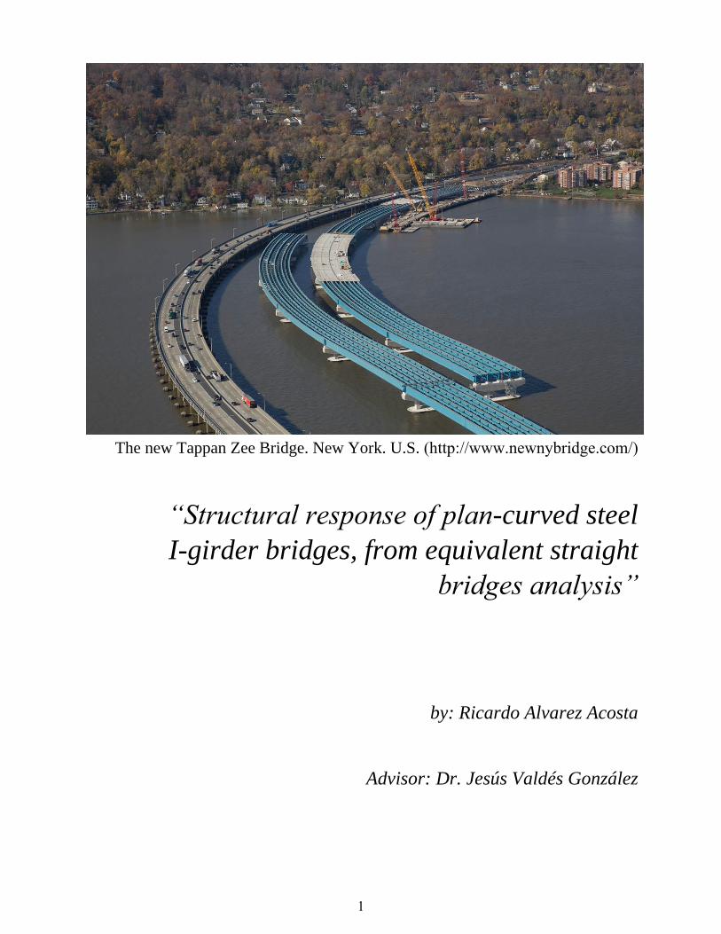
The new Tappan Zee Bridge. New York. U.S. (http://www.newnybridge.com/)
“Structural response of plan-curved steel
I-girder bridges, from equivalent straight
bridges analysis”
by: Ricardo Alvarez Acosta
Advisor: Dr. Jesús Valdés González
1


Structural Response of Plan-curved Steel I-girder Bridges from Equivalent Straight Bridges Analysis
Ricardo Alvarez-Acosta1 and Jesús Valdés-González2
Abstract: A set of equations are developed to estimate the maximum mechanical elements and mid-span deflections of plan-curved
steel I-girder bridges. These formulas are obtained from a statistical correlation analysis based on the results of 60 tridimensional finite-
element models corresponding to different 3-spans continuous curved bridges. The parameters that varied from one model to another
were: curvature radius, span length and number of girders (i.e. load lanes). Two different live load models were separately studied; the
HL-93 and the IMT 66.5. The proposed formulas estimate the maximum mechanical elements of girders, such as: positive and negative
bending moments around the major and minor axis of girders, the vertical shear force, the torsional moment and the deflection at the
mid-span of girders, as a function of the results corresponding to an equivalent straight bridge. Different formulas are proposed for
interior, intermediate and exterior girders in accordance with the bridge cross-section and also for central and extreme girders in
accordance with the span where the girder is located. For each bridge model, the maximum mechanical elements and mid-span
deflections were normalized with respect to the corresponding results of an equivalent straight bridge with the same characteristics of
the curved bridge (span lengths and number of girders), but with a curvature radius equal to ∞. The accuracy of the proposed formulas
was tested for different bridge models to those used in the correlation analysis and the results show that they are accurate enough to be
used with design purposes. In some cases, they resulted more accurate than current applicable formulas and procedures recommended
in the literature.
Introduction
Horizontally curved bridges (CB) are one of the most useful
alternatives to solve complex interchanges of highways.
Currently, the CB constitute a very significant portion of the
built steel bridges. In the United States, the CB represent almost
25% of the total steel bridges which were built until the
beginning of this century (SSRC 1991). The superstructure of
CB is usually structured with steel I-girders which support a
reinforced concrete deck slab. In most of the cases, the girders
are interconnected with steel cross frames in V- or X- type
shapes. Usually, the cross frames provide a relatively high
torsional stiffness to the CB cross-sections. In comparison with
the straight bridges (SB), the CB have a less uniform structural
response of girders in terms of mechanical elements, such as
shear force, bending and torsional moments. In some cases, this
behavior is particularly amplified. This is one of the most
important concerns in the understanding of the structural
behavior of CB. The design of SB does not require refined
analysis models due to most codes provide approximate
methods of analysis which are in most cases reliable. The SB
girders are usually designed using distribution factors to
compute the bending moment and shear force, by considering
the obtained forces from the influence lines of the live load lanes
(AASHTO 2014).
Different bridge design specifications have provided guidelines
for the design of CB (AASHTO 2003 and 2014), however, these
recommendations are based on the analysis of a reduced number
of study cases. This is one of the most important disadvantages
of these simplified methods recommended for the design of CB.
During last years, some studies related to CB have been
conducted. Linzell et al. (2004) as well as Lin and Yoda (2010)
1 Formerly, Graduate Student, School of Engineering, Autonomous
Univ. of the State of Mexico, Cerro de Coatepec s/n, Toluca 50130,
Estado de Mexico. E-mail: [email protected] 2 Professor, School of Engineering, Autonomous Univ. of the State
of Mexico, Cerro de Coatepec s/n, Toluca 50130, Estado de Mexico.
E-mail: [email protected]
presented a historical overview about specifications related to
the design and analysis of CB. The authors argue that in contrast
to SB, CB tend to transmit an important fraction of their loads to
the convex side of the bridge. As a result, they suggest the
analysis of complex 3D structural models representative of the
CB superstructure to understand their behavior. In contrast, the
authors comment that the girders of SB can be modeled
independently one from each other (2D model). Zhang et al.
(2005) determined formulas for live load distribution in
continuous multi-span CB. The most important parameters
taken into consideration in their study were: curvature radius,
number of girders, girder spacing, slab overhang, span length,
slab thickness, girder longitudinal bending inertia, and girder
bending stiffness to overall bridge bending stiffness ratio. In
spite of different parameters were studied, they only analyzed
cases with two lane loads. Furthermore, the study cases were
modeled as a generalized grillage beam system. The obtained
results showed that the developed formulas give good results for
the continuous span CB analyzed, particularly in the estimation
of bending moments and shear forces. These estimations were
more accurate than those obtained from the AASHTO (1993)
specifications.
DeSantiago et al. (2005) studied the increase of bending and
torsional moments and deflection of CB, in comparison with SB.
The authors studied over 120 study cases corresponding to
simply supported bridges with different curvature angles (0 to
30º) and different distances between cross frames which varied
from 1/30 of the span length to full span length. The study only
considered a constant span length of 30.4 m. Moreover, the
study cases were modeled with finite element using frame and
plate elements. The results showed that the deflection of girders
of CB can be about 1.2 to 4.2 times higher than in girders of SB.
The bending and torsional moments can be about 8.7 % to
23.5 % higher and 3.7 % to 10.3 %, respectively, compared with
moments in SB girders.
Other studies were made by Nevling at al. (2006) to evaluate the
accuracy of different levels of analysis used to predict CB
3

response. A similar research was made by Kim et al. (2007), they
evaluated simply supported CB. The study was made using 3
numerical models which were updated using field test results.
This research showed that curvature radius, span length, spacing
of girders and cross frames are the most significant parameters
in the response of CB. As a result of this research, correlation
formulas to compute the normal stress and a combined treating
bending and warping normal stress separately were proposed.
The formulas had a correlation coefficient of 0.92 and showed
better results than the AASHTO (1993) specifications.
Barr et al. (2007) focused on a three-span curved steel I-girder
bridge which was tested under three boundary condition states
to determine its response to live load. They found that the
V-load method specified in AASHTO recommendations were
unconservative. Fatemi et al. (2015) made a parametric study
using a proposed analytical model to investigate the effect of
various parameters such as curvature ratio, span length, number
of cells and number of loading lanes on bending moment and
torsion of the curved bridges subjected to Australian bridge
design loads. The currently AASHTO bridge design
specifications (AASHTO LRFD 2014) mention a simplified
method (V-Load) for the analysis of CB. In this method, the
curved girders are represented by equivalent straight girders and
the effects of curvature are represented by vertical and lateral
forces applied at the cross-frame locations. Meanwhile, the
Canadian Highway Bridge Design Code (CHBDC 2006)
consider that the behavior of CB is similar to SB, in case that the
quotient of the square span length (L2) divided by the product of
the bridge width (B) and curvature radius (R) is either less than
or equal to 0.5, L2/(BR)≤0.5. This limit value of 0.5 was
considered as 1.0 in previous specifications (CHBDC 2000).
These limitations were evaluated under dead load by Khalafalla
and Sennah (2014). Results proved that such code limitations
were unsafe and empirical expressions were developed to
determine such limitations more accurately and reliably.
The research made by Al-Hashimy (2005) consisted in the
analysis of 320 simply supported CB and SB models, taking into
account the variation of curvature radius, distance between cross
frames, number of girders, girder spacing and span length.
Models were analyzed with FEM to evaluate their structural
response considering the live load specified by the CHBDC
(2000). As a result, a set of empirical expressions were obtained
to estimate shear forces, bending moments, warping to bending
stress ratios in steel flanges and deflection in interior, middle and
exterior girders, for both, SB and CB. The results showed that it
is not adequate to deal with CB as if they were SB in accordance
with the CHBDC (2000). In this case, it was demonstrated that
the CHBDC significantly underestimated the moment
distribution factors in CB girders, under the assumption that CB
may be analyzed as if they were SB.
There are different formulas to estimate the structural behavior
of CB in the AASHTO specifications and different
aforementioned studies. However, each one was obtained
considering particular conditions. So, it is important to study a
larger number of cases to have a more complete view of the
problem that represent the distribution of bridge live loads and
deflections in the CB girders.
In the current study, several finite element models representative
of three-spans continuous curved bridges are analyzed. Different
curvature radii (60 m to 280 m), span lengths (20 to 60 m) and
number of girders (2 to 6) were studied. The results for these
models are statistically analyzed and correlation models are
evaluated. These correlation models relate the studied variables
to the modification factor of live loads in CB girders for different
mechanical elements (bending moment, vertical shear force and
torsional moment) and deflection of girders. The proposed
correlation formulas have an average error of 5 % with a
variation ranging from 0 % to 16 %. The correlation analysis
reported a RMSE (root main square error) that varies from
0.005 % to 18 % and a correlation coefficient (R2) that ranges
from 0.82 to 0.99, for the different obtained formulas. In
addition, the correlation models are tested using different cases
to those used in the correlation analysis. In comparison with the
proposed formulas by Zhang et al. (2005) and the AASHTO
LRFD (2014) specifications (V-load method) to estimate the
bending moment and the shear force in CB girders, it was
demonstrated that, in general, the proposed formulas in this
study give smaller errors than those obtained using cited existing
formulas and procedures. The study is done to consider two
different live load models, the HL-93 (AASHTO LRFD 2014)
and the IMT 66.5 (SCT 2001). Results for both live load models
are similar.
Bridge models
A particular two load lane bridge was considered as a base to
generate the bridge models (BM) that were studied (Fig. 1). The
bridge is a structure composed with two longitudinal steel
I-girders separated 5.5 m each other that support a concrete deck
slab of 230 mm with a slab overhang of 1.50 m. The bridge has
seven continuous spans with radial supports and different span
lengths (L) that vary from 27 m to 60.35 m with a total bridge
length of 342 m. The bridge has a curvature radius equal to
284.25 m measured along bridge centerline. The steel I-girders
have a depth of 2,416 mm and a width of 900 mm with a
thickness of 16 mm in the web and 38 mm in the flanges.
A total number of 60 different three-span continuous BM were
analyzed. The supports were radial and did not have any
elevation variation. The parameters that varied from one model
to other were: curvature radius (R), span length (L) and number
of girders (N). For each model, it is assumed that the number of
Fig. 1. Actual bridge that was taken as a base to generate the studied models
4

loaded lanes is equal to the number of girders. The total number
of models was obtained considering the combination of 4
curvature radii, 5 span lengths and 3 superstructure bridge
cross-sections corresponding each one to a different number of
girders. The table 1 shows the adopted values for each parameter
Table 1. Range of parameters for the studied models
Parameter Range
Curvature Radius [m] 60, 170, 280, ∞
Span Length [m] 20, 30, 40, 50, 60
Number of Girders 2, 4, 6
The 3D finite element models (FEM) were created using the
CSIBridge software (CSI 2016). The deck, girders flanges and
girders web were modeled using shell elements while cross
frames were modeled with frame elements. Fig. 2 shows one of
the studied 3D FEM. Fig. 3 shows the geometry details for the
different bridge superstructure cross-sections used in the
analyzed models. The distance between cross frames was equal
to L/10 for all cases.
The depth of the girders in the different models was chosen to
guarantee that the bending stress was similar in all models. The
configuration of spacing cross frame and supports is shown in
Fig. 4.
Fig. 2. An example of the 3D finite element BM used in the
analysis
For the present study, two types of live load were analyzed:
HL-93 (AASHTO 2014) and IMT 66.5 (SCT 2001). IMT 66.5
is a live load model that consists of a design truck and a design
lane load. The design truck has a total weight of 66.5 t. For span
lengths larger than 30 m, the total weight is divided in three
different axle loads: P1 = 5 t, P2 = 24 t and P3 = 37.5 t. The
distance between P1 and P2 is equal to 5 m, while P2 and P3 have
a distance of 9 m. The design lane load consists of a load
w = (30-L)/60.t/m, uniformly distributed over a 3 m lane width.
The transverse spacing of wheels was taken as 1.8 m. For span
lengths less than 30 m, w = 0 and the axle loads are P1 = 5 t,
(a) (b)
(c)
Fig. 3. Bridge cross-sections used in the analyzed models: (a) bridge cross-section for models with 2 girders; (b) bridge cross-section for
models with 4 girders; (c) bridge cross-section for models with 6 girders
Fig. 4. Plan view of studied CB
5

0.8
0.9
1.0
1.1
1.2
1.3
1.4
1.5
0.0 0.1 0.2 0.3 0.4 0.5 0.6 0.7 0.8 0.9 1.0 1.1
MF
L/R
1.0
1.1
1.2
0.0 0.1 0.2 0.3 0.4 0.5 0.6 0.7 0.8 0.9 1.0 1.1
MF
L/R
0.2
0.4
0.6
0.8
1.0
1.2
1.4
1.6
1.8
2.0
2.2
0.0 0.1 0.2 0.3 0.4 0.5 0.6 0.7 0.8 0.9 1.0 1.1
MF
L/R
1.0
1.1
1.2
1.3
1.4
1.5
0.0 0.1 0.2 0.3 0.4 0.5 0.6 0.7 0.8 0.9 1.0 1.1
MF
L/R
P2 = P3 = 12 t and P4 = P5 = P6 = 12.5 t. In this case the distances
between the axle loads are equal to 4.4 m from P1 to P2, 1.2 m
from P2 to P3, 7.2 m from P3 to P4, 1.2 m from P4 to P5 and
1.2 m from P5 to P6 as well. In addition, the multiple presence
factors as specified in AASHTO LRFD 2014 were included in
the analysis, in order to obtain the most critical response.
Parametric results analysis
According to the maximum responses obtained from the analysis
of each model, different mechanical elements and vertical
deflections of the bridge superstructure were identified. The
results were classified in extreme and central spans, T1 and T2
respectively (Fig. 4). The studied mechanical elements were:
vertical shear force (V), positive and negative bending moments
around major axis (𝑀33+ , 𝑀33
− ), lateral bending moment (M22) and
torsional moment (T). Also, the vertical deflection at the mid
span (Δ) was studied. The modification factor (MF) was
obtained by dividing the maximum response of CB (RCB) by the
maximum response of the equivalent SB (RSB). The equivalent
SB has the same characteristics of CB such as span length and
bridge cross-section, but it has a curvature radius equal to ∞. The
MF was obtained for interior, intermediate and exterior girders
in accordance to Eq. (1).
𝑀𝐹 =𝑅𝐶𝐵
𝑅𝑆𝐵 (1)
The behavior of different MF can be observed in plots of Figs.
5-10, which show the MF values for responses of T1 considering
the HL-93 live load model. The horizontal axis shows the span
length to curvature radius ratio values (L/R) and the vertical one
the corresponding to MF value. Plots for T2 are similar to T1
plots.
Fig. 5 shows the MF values computed for the vertical shear force
(V). Fig. 5a shows the values for interior and exterior girders.
For interior girders, the MF values are practically lower than
1.00 and reach a minimum value of 0.85, while for exterior
girders the MF values are higher than 1.00 and reach values
close to 1.50. For models with 4 and 6 girders the variation of
MF as a function of L/R is almost linear for both cases, interior
and exterior girders; while for models with 2 girders, the
variation is parabolic for L/R values higher than 0.50. Fig. 5b
shows the MF for intermediate girders (models with 4 and 6
girders). In this case, the MF increases linearly with the increase
of L/R and varies from 1.00 to 1.15 approximately.
Fig. 6 shows the MF values computed for the positive bending
moment (𝑀33+ ). Fig. 6a shows the values for interior and exterior
girders. For interior girders, the MF varies linearly from 1.00 to
0.42, the values of MF decrease for increasing values of L/R. For
exterior girders, the MF is higher than 1.00 and reach a
maximum value of 2.15, the values of MF increase for
increasing values of L/R. For intermediate girders (Fig. 6b), the
MF values are higher than 1.00 and reach a maximum value of
1.50 with a linear variation from L/R = 0.07 to 0.85,
approximately.
(a) (b)
Fig. 5. MF for vertical shear force (V): (a) interior and exterior girders; (b) intermediate girder
(a) (b)
Fig. 6. MF for positive bending moment (𝑀33+ ): (a) interior and exterior girders; (b) intermediate girder
- - - - - - Interior girder _______ Exterior girder
• 4 girders
x 6 girders
― ⋅ ― ⋅ ― Intermediate girder
▲ 2 girders
• 4 girders
x 6 girders
▲ 2 girders
• 4 girders
x 6 girders
• 4 girders
x 6 girders
- - - - - - Interior girder _______ Exterior girder ― ⋅ ― ⋅ ― Intermediate girder
6
0.6
0.8
1.0
1.2
1.4
1.6
1.8
0.0 0.1 0.2 0.3 0.4 0.5 0.6 0.7 0.8 0.9 1.0 1.1
MF
L/R
0.9
1.0
1.1
1.2
1.3
1.4
1.5
1.6
1.7
0.0 0.1 0.2 0.3 0.4 0.5 0.6 0.7 0.8 0.9 1.0 1.1
MF
L/R
0.6
0.8
1.0
1.2
1.4
1.6
1.8
2.0
2.2
0.0 0.1 0.2 0.3 0.4 0.5 0.6 0.7 0.8 0.9 1.0 1.1
MF
L/R
0.8
1.0
1.2
1.4
1.6
1.8
2.0
2.2
2.4
2.6
0.0 0.1 0.2 0.3 0.4 0.5 0.6 0.7 0.8 0.9 1.0 1.1
MF
L/R
0.5
1.0
1.5
2.0
2.5
3.0
3.5
4.0
4.5
5.0
5.5
6.0
0.0 0.1 0.2 0.3 0.4 0.5 0.6 0.7 0.8 0.9 1.0 1.1
MF
L/R
0.5
1.0
1.5
2.0
2.5
3.0
3.5
4.0
4.5
0.0 0.1 0.2 0.3 0.4 0.5 0.6 0.7 0.8 0.9 1.0 1.1
MF
(a) (b)
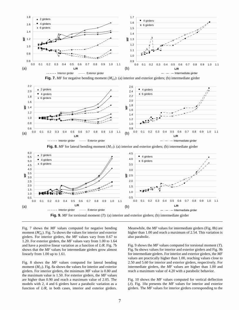
Fig. 7. MF for negative bending moment (𝑀33− ): (a) interior and exterior girders; (b) intermediate girder
(a) (b)
Fig. 8. MF for lateral bending moment (M22): (a) interior and exterior girders; (b) intermediate girder
(a) (b)
Fig. 9. MF for torsional moment (T): (a) interior and exterior girders; (b) intermediate girder
Fig. 7 shows the MF values computed for negative bending
moment (𝑀33− ). Fig. 7a shows the values for interior and exterior
girders. For interior girders, the MF values vary from 0.67 to
1.20. For exterior girders, the MF values vary from 1.00 to 1.64
and have a positive linear variation as a function of L/R. Fig. 7b
shows that the MF values for intermediate girders grow almost
linearly from 1.00 up to 1.61.
Fig. 8 shows the MF values computed for lateral bending
moment (M22). Fig. 8a shows the values for interior and exterior
girders. For interior girders, the minimum MF value is 0.80 and
the maximum value is 1.50. For exterior girders, the MF values
are higher than 0.90 and reach a maximum value of 2.05. The
models with 2, 4 and 6 girders have a parabolic variation as a
function of L/R, in both cases, interior and exterior girders.
Meanwhile, the MF values for intermediate girders (Fig. 8b) are
higher than 1.00 and reach a maximum of 2.54. This variation is
also parabolic.
Fig. 9 shows the MF values computed for torsional moment (T).
Fig. 9a shows values for interior and exterior girders and Fig. 9b
for intermediate girders. For interior and exterior girders, the MF
values are practically higher than 1.00, reaching values close to
2.50 and 5.60 for interior and exterior girders, respectively. For
intermediate girders, the MF values are higher than 1.00 and
reach a maximum value of 4.20 with a parabolic behavior.
Fig. 10 shows the MF values computed for vertical deflection
(Δ). Fig. 10a presents the MF values for interior and exterior
girders. The MF values for interior girders corresponding to the
- - - - - - Interior girder _______ Exterior girder
- - - - - - Interior girder _______ Exterior girder
- - - - - - Interior girder _______ Exterior girder
― ⋅ ― ⋅ ― Intermediate girder
― ⋅ ― ⋅ ― Intermediate girder
L/R
― ⋅ ― ⋅ ― Intermediate girder
• 4 girders
x 6 girders
• 4 girders
x 6 girders
• 4 girders
x 6 girders
▲ 2 girders
• 4 girders
x 6 girders
▲ 2 girders
• 4 girders
x 6 girders
▲ 2 girders
• 4 girders
x 6 girders
7

0.0
1.0
2.0
3.0
4.0
5.0
6.0
7.0
8.0
0.0 0.1 0.2 0.3 0.4 0.5 0.6 0.7 0.8 0.9 1.0 1.1
MF
L/R
1.0
1.5
2.0
2.5
3.0
3.5
4.0
4.5
5.0
0.0 0.1 0.2 0.3 0.4 0.5 0.6 0.7 0.8 0.9 1.0 1.1
MF
(a) (b)
Fig. 10. MF for vertical deflection (): (a) interior and exterior girders; (b) intermediate girder
models with 4 and 6 girders, are practically lower than 1.00
(0.50 to 0.92). In this case, the MF as a function of L/R has a
negative linear variation. However, the MF for interior girders
corresponding to the models with 2 girders varies from 1.00 to
3.50 and exhibits a parabolic behavior. In addition, for exterior
girders the MF values are higher than 1.00 and reach a
maximum value of 7.36 with a parabolic variation in all cases.
Meanwhile, Fig. 10b shows the MF values for intermediate
girders, which vary from 1.00 to 4.50 with a parabolic behavior.
As a summary of the MF values, Table 2 shows the maximum
and minimum MF values for extreme values of L/R ratios
corresponding to the extreme spans (T1 in Figs. 5-10) and the
corresponding to the central span (T2). These values represent
the range in which the MF can vary for each girder taking into
account the value of: L, R and N. It can be seen that the MF
value increases significantly from interior to exterior girder.
Table 2. Summary of maximum and minimum MF values for
T1 and T2
Structural
response
Exterior
girder
Intermediate
girder
Interior
girder
Max Min Max Min Max Min
T1
V 1.465 1.025 1.157 1.026 1.158 0.838
𝑀33+ 2.142 1.035 1.496 1.012 0.965 0.423
𝑀33− 1.644 1.032 1.613 1.016 1.230 0.667
M22 2.050 0.890 2.547 1.005 1.481 0.788
T 5.577 0.909 4.163 1.032 2.450 0.895
Δ 7.368 1.069 4.425 1.034 3.522 0.491
T2
V 1.239 1.024 1.327 0.872 1.135 1.025
𝑀33+ 1.903 1.030 0.968 0.574 1.352 1.010
𝑀33− 1.720 1.031 1.227 0.616 1.604 1.017
M22 1.852 0.939 1.609 0.876 1.866 0.994
T 4.737 1.033 2.892 0.940 3.999 1.073
Δ 7.471 1.061 3.559 0.489 4.493 1.032
Correlation analysis
Considering the obtained results from the analysis of the 60
models, some expressions were developed to relate the
different MF with the variables involved in the analysis (span
length, curvature radius and number of girders).
A correlation analysis was made considering basic formulas
defined by the Eqs. (2) and (3). Eq. (2) was used for all mecha-
nical elements and superstructure deflection, except for the case
of torsional moment in interior girders, which was analyzed
with Eq. (3).
𝑀𝐹 = 𝑎 (𝐿
𝑅)
𝑏
𝑁𝑐 +(
𝐿
𝑅)
𝑑
𝑁𝑒 𝑓 + 𝑔 (2)
𝑀𝐹T (interior girder) = ℎ (𝐿𝑖
𝑅) + 𝑗 (3)
where a to j are the coefficients obtained through the correlation
analysis and L, R and N are the variables corresponding to the
geometry of the analyzed models, span length, curvature radius
and number of girders, respectively.
The coefficient values were obtained taking into account the
best correlation coefficient (R2) and the minimum root mean
square error (RMSE) for each formula. Some similar correlation
models were used by Khalafalla and Sennah (2014) and
Al-Hashimy (2005) to estimate the magnification factors for
dead and live load and for both SB and CB under limitations of
CHBDC by treating CB as SB.
Tables 3 and 4 show the correlation analysis corresponding to
different mechanical elements and to deflection of
superstructure for interior, intermediate and exterior girders due
to HL-93 live load. Column 4 shows the R2 and column 5 the
corresponding to RMSE. Table 3 is associated to the results of
Eq. (2) and Table 4 to the results of Eq. (3).
For Eq. (2) (Table 3), the maximum R2 and RMSE were 0.99
(99 %) and 0.18 (18 %), respectively; while the minimum
values were 0.82 (82 %) and 0.006 (0.6 %), respectively. For
Eq. (3) (Table 4), the R2 were 0.88 (88 %) and 0.94 (94 %),
while the RMSE were 0.12 (12 %) and 0.10 (10 %) for T1 and
T2, respectively. These values show the accuracy of the
proposed formulas.
The best fit corresponds to the formulas for the computation of
T and Δ which have a R2 average values of 0.95 (95%) and 0.99
(99%), respectively. Meanwhile, the worst fit corresponds to
the formulas for the calculation of V and M22. In this case, the
average values for R2 were 0.92 and 0.93. In spite of the best
and worst fits, the minimum RMSE average value corresponds
to the formulas for V, 𝑀33+ and 𝑀33
− with: 0.013(1.3%), 0.032
(3.2%) and 0.032(3.2%), respectively. In general, the best fit
corresponds to intermediate girders.
▲ 2 girders
• 4 girders
x 6 girders
• 4 girders
x 6 girders
L/R
― ⋅ ― ⋅ ― Intermediate girder- - - - - - Interior girder _______
Exterior girder
8

Table 3. Coefficient values for the proposed correlation formulas (Eq. 2)
Structural
response Girder R2 RMSE
Coefficient Values
a b c d e f g
V
Interior T1 0.87 0.017 -0.3801 2.318 -0.1067 3.948 1 1 0.9773
T2 0.97 0.011 -1.888 3.324 -0.6087 4.103 1 3.163 0.9793
Intermediate T1 0.98 0.005 -3.521 0.6173 -2.344 1.071 1 1 1.04
T2 0.96 0.006 -2.639 0.6376 -2.006 0.998 1 1 1.042
Exterior T1 0.92 0.021 -0.0931 2.916 0.1238 2.939 1 1 1.046
T2 0.82 0.016 -0.4684 3.415 -0.5559 3.038 1 1 1.042
𝑴𝟑𝟑+
Interior T1 0.93 0.038 -1.55 0.8149 -0.4791 0.9093 1 1 1.033
T2 0.87 0.037 -0.9321 1.11 -0.4377 5.208 1 1 0.9782
Intermediate T1 0.98 0.017 0.0757 0.6834 0.8229 9.834 1 1 0.9719
T2 0.98 0.012 0.03272 6.497 0.9364 0.05768 -0.069 1 0.04372
Exterior T1 0.95 0.048 0.7529 0.7762 -0.2108 15.45 1 1 0.9633
T2 0.95 0.040 0.6012 0.375 -0.0662 6.878 1 1 0.8184
𝑴𝟑𝟑−
Interior T1 0.90 0.030 -0.2274 0.6583 0.3938 4.334 1 1 1.033
T2 0.97 0.019 12.64 2.95 -4.629 0.6206 -0.241 -0.280 1.043
Intermediate T1 0.93 0.043 0.1924 0.5332 0.5829 4.087 1 1 0.902
T2 0.99 0.015 0.1877 0.7798 0.5242 4.651 1 1 0.9616
Exterior T1 0.93 0.038 0.1158 0.4181 0.6412 0.8132 1 1 0.9032
T2 0.89 0.045 0.0753 0.444 0.7476 0.9844 1 1 0.9523
M22
Interior T1 0.87 0.039 -0.127 0.6169 0.6241 1.545 1 1 1.066
T2 0.90 0.038 -0.0675 0.1689 0.7716 8.241 0.6881 0.9533 1.144
Intermediate T1 0.97 0.062 1.356 13.2 -0.378 0.5452 0 1 0.7473
T2 0.97 0.038 0.00782 7.368 2.135 1.024 0.6371 1.702 0.966
Exterior T1 0.91 0.066 0.1979 1.499 1.006 -0.0833 0 1 -0.2183
T2 0.96 0.044 0.9913 1.774 0.05898 0.95 1 -1.243 1.025
T
Intermediate T1 0.97 0.140 3.091 1.962 -0.2852 8.205 0.1561 1 1.139
T2 0.99 0.081 4.944 2.335 -0.6481 19.91 0.177 1 1.137
Exterior T1 0.97 0.180 2.268 5.584 0.227 0.4052 -0.289 1 0.4842
T2 0.95 0.180 1.326 1.932 0.242 8.22 -0.2 1 1.11
Δ
Interior T1 0.97 0.074 -11.79 2.724 -0.6326 3.311 1 20.26 0.8628
T2 0.99 0.046 -0.1034 0.7697 1 6.436 2.69 18.51 0.9364
Intermediate T1 0.99 0.081 1.871 1.786 0.06357 13.39 -0.105 1 1.068
T2 0.99 0.096 1.929 1.888 -0.0037 9.979 -0.201 1 1.084
Exterior T1 0.99 0.140 11.42 6.186 -1.2 1.142 -0.392 1 1.06
T2 0.99 0.140 1.561 0.952 0.1134 7.13 1 9.603 0.9215
Note: R2=Correlation coefficient; RMSE=Root main square error; T1=Extreme span; T2=Central span.
Table 4. Coefficient values for the proposed correlation formulas (Eq. 3)
Note: R2=Correlation coefficient; RMSE=Root main square error; T1=Extreme span; T2=Central span; N=Number of girder
Evaluation of proposed formulas
In order to evaluate the efficiency of the proposed formulas, two
different CB, which were not included in the 60 analyzed models
used to obtain the correlation formulas, were analyzed. The
analysis was made by comparing the results of a 3D FEM with
those obtained using the proposed formulas in this paper and
also with different formulas and procedures proposed in the
literature.
The first curved bridge (CB1) has a cross-section with three
girders, a curvature radius of 120 m, a span length of 45 m and
3 live load lanes. The second one (CB2) has five girders, a
curvature radius of 225 m, a span length of 45 m and 5 live load
lanes. In both cases, the slab overhang was 1.50 m and the slab
thickness was 0.23 m. Fig. 11 shows the 3D FEM used in the
analysis of CB1 and CB2 (CSI, 2016). Figs. 12 and 13 shows
the geometry details of both bridges.
Fig. 11. 3D FEM of CB used to test the proposed formulas
Structural
response Girder R2 RMSE
Coefficient Values
h i j
T Interior T1 0.88 0.120 0.001 -0.0116N2 + 0.0653N + 2.688 -0.0002N2 + 0.0279N + 0.7884
T2 0.94 0.100 0.004 -0.0058N2 + 0.0225N + 2.462 0.01N2 - 0.1049N + 1.1377
9

(a) (b)
Fig. 12 Superstructure cross-sections: (a) superstructure cross-section for CB1; (b) superstructure cross-section for CB2
(a) (b)
Fig. 13. Models in a plan view: (a) plan view of CB1; (b) plan view of CB2
In the following discussion of results, the differences were
computed between the results obtained from proposed formulas
and those from the 3D FEM. A positive difference means an
overestimated response value and a negative one, an
underestimated response value. Moreover, the averages
involved in the discussion of the results were computed as the
root of the average of the square differences.
Table 5 shows the results for CB1. The column 4 shows the MF
(Eq.1) obtained from the analysis of the 3D FEM, the column 5
shows the MF computed using the proposed formulas and the
column 6 presents the difference between them. In the case of
T1, the minimum difference is 0.4 % corresponding to V, while
the maximum difference is 16.1 % which corresponds to T. In
the case of T2, the minimum difference is 0.3 % corresponding
to M22 and the maximum difference is 13.9 % which corresponds
to Δ. The results for V and M22 have the minimum average of
differences, 3.1 % and 4.25 %, respectively. While the
maximum average of differences occurs for T and it is 10.6 %.
Table 6 shows the results for CB2. The order and identification
of the columns is the same as Table 5. In the case of T1, the
minimum difference is 0.6 % corresponding to T and Δ, while
the maximum difference is 8.8 % which corresponds to Δ. In the
case of T2, the minimum difference is 0.2 % corresponding to V
and the maximum difference is 6.3 % which corresponds to Δ.
The results for V and M22 have the minimum average of
differences, 1.5 % and 2.5 %, respectively. While the maximum
average of differences occurs for Δ and it is 4.8 %.
In general, the minimum differences correspond to girders
located in the central span of the bridge (T2) for both models,
CB1 and CB2. From the obtained results for both bridges, it can
be seen that the proposed formulas give close estimations for
different MF to those obtained from the 3D FEM.
In addition, the results were compared with different simplified
formulas and procedures proposed in the literature. The CHBDC
(2006) establishes that a CB can be analyzed as a SB in case that
the L2/BR≤0.50. Under this consideration, the CB1 cannot be
considered as a SB, but CB2 can be. The results for CB2 show
that following the recommendation of CHBDC, in which case
MF = 1.00 should be assumed for all mechanical elements and
deflection, the differences between the 3D FEM and those.
Table 5. Results summary for CB1
MF
Structural Girder
response FEM
Proposed
formulas Difference
V
Interior T1 0.882 0.949 7.1 %
T2 0.947 0.961 1.5 %
Intermediate T1 1.020 1.010 -1.0 %
T2 1.018 1.011 -0.6 %
Exterior T1 1.063 1.059 -0.4 %
T2 1.055 1.050 -0.4 %
𝑀33+
Interior T1 0.848 0.758 -12.0 %
T2 0.794 0.786 -1.0 %
Intermediate T1 1.038 1.068 2.8 %
T2 1.002 1.064 5.8 %
Exterior T1 1.167 1.242 6.1 %
T2 1.178 1.206 2.3 %
𝑀33−
Interior T1 0.865 0.854 -1.3 %
T2 0.876 0.849 -3.2 %
Intermediate T1 1.070 1.124 4.8 %
T2 1.062 1.120 5.2 %
Exterior T1 1.170 1.209 3.2 %
T2 1.164 1.190 2.2 %
M22
Interior T1 0.972 1.002 2.9 %
T2 1.014 1.011 -0.3 %
Intermediate T1 1.208 1.333 9.4 %
T2 1.266 1.276 0.7%
Exterior T1 1.026 1.004 -2.1 %
T2 1.073 1.047 -2.4 %
T
Interior T1 1.352 1.198 -12.8 %
T2 1.381 1.328 -4.0 %
Intermediate T1 1.705 1.469 -16.1 %
T2 1.370 1.383 0.9 %
Exterior T1 1.579 1.420 -11.2 %
T2 1.514 1.370 -10.5 %
Δ
Interior T1 0.776 0.719 -8.0 %
T2 0.730 0.792 7.9 %
Intermediate T1 1.221 1.416 13.7 %
T2 1.193 1.386 13.9 %
Exterior T1 1.515 1.569 3.4 %
T2 1.545 1.619 4.6 %
10

Table 6. Results summary for CB2
MF
Structural Girder
response FEM
Proposed
formulas Difference
V
Interior T1 0.978 0.970 -0.8 %
T2 0.979 0.977 -0.2 %
Intermediate T1 1.027 1.046 1.8 %
T2 1.026 1.045 1.8 %
Exterior T1 1.026 1.047 2.0 %
T2 1.024 1.043 1.8 %
𝑀33+
Interior T1 0.924 0.886 -4.2 %
T2 0.914 0.901 -1.5 %
Intermediate T1 1.055 1.067 1.1 %
T2 1.052 1.063 1.0 %
Exterior T1 1.078 1.117 3.5 %
T2 1.082 1.114 2.9 %
𝑀33−
Interior T1 0.916 0.885 -3.5 %
T2 0.920 0.891 -3.2 %
Intermediate T1 1.075 1.111 3.2 %
T2 1.074 1.086 1.1 %
Exterior T1 1.090 1.123 2.9 %
T2 1.083 1.116 3.0 %
M22
Interior T1 0.946 0.954 0.9 %
T2 0.975 0.966 -0.9 %
Intermediate T1 1.101 1.163 5.3 %
T2 1.092 1.083 -0.8 %
Exterior T1 1.040 1.015 -2.5 %
T2 1.041 1.034 -0.7 %
T
Interior T1 0.994 1.065 6.7 %
T2 1.026 1.048 2.1 %
Intermediate T1 1.286 1.222 -5.2 %
T2 1.199 1.178 -1.8 %
Exterior T1 1.219 1.315 7.3 %
T2 1.205 1.197 -0.6 %
Δ
Interior T1 0.825 0.829 0.6 %
T2 0.818 0.787 -4.0 %
Intermediate T1 1.178 1.185 0.6 %
T2 1.170 1.176 0.5 %
Exterior T1 1.239 1.359 8.8 %
T2 1.242 1.326 6.3 %
obtained considering CHBDC (2016), could be as high as 29 %
for T and 24 % for . While in the case of computing the MF for
T and using the proposed formulas in this paper, these
differences were 5.2 % and 6.3 %, respectively.
Moreover, the AASHTO guide for curved bridges (AASHTO
2003) and AASHTO bridge design specification (AASHTO
LRFD 2014) provide some conditions to ignore the effects of
curvature for determining the bending moment and shear forces.
These conditions are: girders are concentric, bearing lines are
not skewed more than 10 degrees, the stiffnesses of the girders
are similar and for all spans, the arc span (Las) divided by the
curvature radius (R) is less than 0.06 radians, where the arc span
(Las), shall be taken in accordance with the support conditions.
When these conditions are not satisfied, the specifications
recommend an approximate method, which is the V-Load
method. This method allows to compute the mechanical
elements in the girders of the equivalent straight bridge either
use the distribution factors specified in the AASHTO LRFD
specifications (2014) or use the lever rule.
Additionally, the obtained results using the proposed formulas
were compared with the formulas proposed by Zhang et al.
(2005) and with the results from V-load method, the procedure
recommended by AASHTO (2003, 2014).
According to these recommendations, the vertical shear force
(V) and the bending moments (𝑀33+ , 𝑀33
− ) were computed for
CB1 and CB2. Table 7 shows the differences between the
V-load method, the formulas proposed by Zhang et al. (2005)
and those obtained with the proposed formulas in this paper. For
all three cases, the differences were obtained by comparing the
results of the 3D FEM with the resulting values in each
procedure. For CB1, the difference of V-load method reached
values as high as -57.1% for 𝑀33+ , while the minimum difference
was about 10% for 𝑀33+ (exterior girder). In the case of CB2, the
difference for V by using the V-load method was about
-11.2%, and the minimum difference was 0.9% for 𝑀33− .
Particularly, Zhang et al. (2005) propose formulas for the
computation of V, 𝑀33+ and 𝑀33
− which are applicable to
continuous bridges with multiple live load lanes. The column 6
of Table 7 shows the differences between the MF computed
using the proposed formulas by Zhang et al. (2005) and those
obtained from the analysis of the 3D FEM. These differences
can reach maximum values of 13.6 % for CB1 (𝑀33+ ) and
minimum values of -1.3 % (CB2) when V is computed in interior
girders. For CB1 the average difference was 9.0 % and for CB2
it was 4.7 %. For the proposed formulas in this paper, the
maximum differences were -12 % (CB1) and -4.2 % (CB2).
While the minimum differences were -0.4 % (CB1) and -0.8 %
(CB2). The average differences for CB1 and CB2 were 6.4 %
and 2.9 %, respectively.
Table 7. Summary results of comparison of different
procedures
Differences
Structural
response Girder
Proposed
formulas
V-Load
method
Zhang et
al. (2005)
CB1
V Interior 7.1 % -33.6 % 7.1 %
Exterior -0.4 % 20.7 % 5.2 %
𝑀33+
Interior -12.0 % -57.1 % -5.8 %
Exterior 6.1 % 12.9 % 13.6 %
𝑀33−
Interior -1.3 % -27.2 % 13.4 %
Exterior 3.2 % 10.7 % -1.8 %
CB2
V Interior -0.8 % -11.2 % -1.3 %
Exterior 2.0 % 7.6 % -1.7 %
𝑀33+
Interior -4.2 % -8.7 % 5.1 %
Exterior 2.9 % -3.0 % 6.4 %
𝑀33−
Interior -3.2 % -2.2 % 6.4 %
Exterior 2.9 % 0.9 % -4.2 %
Comparison between HL-93 and IMT66.5 live load models
By comparing the BM responses for the HL-93 (AASHTO
LRFD 2014) and the IMT66.5 (SCT 2001) live load models, the
results for T1 showed that vertical shear force (V), bending
11

moments (𝑀33+ , 𝑀33
− , M22), and deflection (), have roughly the
same behavior and the same MF values, regardless what live
load is used. However, the torsional moment (T) does not have
the same behavior. In the case of T2, V, 𝑀33+ , 𝑀33
− and Δ also
have the same behavior, while T and M22 have different behavior
in case of using one live load model or another one.
Fig. 14 shows the obtained MF for different L/R ratios that
corresponds to 𝑀33+ considering the 60 analyzed 3D FEM in this
study. It can be seen small differences for IMT 66.5 and HL-93
live load models. Hence, the MF for IMT 66.5 live load can be
considered the same as HL-93.
Fig. 14. Response comparison for 𝑀33+ between HL-93 and IMT
66.5
Fig. 15 shows the behavior of MF corresponding to T for
different L/R ratios. It shows the same behavior, both models
have a parabolic behavior as a function of L/R. However, the MF
values for the IMT 66.5 live load model are lower than HL-93.
For L/R ratios less than 0.20 the MF values can be considered
the same. For L/R ratios higher than 0.30, the MF for HL-93 and
IMT 66.5 live load models increase significantly. The maximum
MF values are 2.45 for IMT 66.5 and 4.10 for HL-93, both cases
occur for L/R = 1.00.
Fig. 15. Response comparison for T between HL-93 and IMT
66.5
Conclusions
Using 60 3D FEM representative of the superstructure of
continuous curved steel I-girder bridges, a set of formulas were
developed to estimate different mechanical elements and
deflections of girders of plan-curved bridges. The parameters
that varied from one model to another were: curvature radius,
span length and number of girders (i.e. load lanes). The formulas
were obtained through a correlation analysis of the results, and
they give a factor that converts the mechanical elements and
deflections of “equivalent” straight bridge girders in the
corresponding ones to girders of a plan-curved bridge. These
formulas were tested using different cases to those used in the
correlation analysis and the results show that they are accurate
enough to be used with design purposes. In many cases, they are
more accurate than current applicable formulas and procedures
recommended in the literature. The main conclusions and
recommendations of this paper are as follows:
1. In general, the variation of the girders response for the 60
analyzed curved bridge FEM ranged from MF = 0.42 to
MF = 7.40. Considering the three different girders type in
accordance with their location in the bridge cross-section,
the girders that resulted with the highest MF values were
the exterior girders, in which case the average value of the
maxima MF considering all different studied responses
was 3.26, while the average value of the minima MF was
1.00. Meanwhile, the girders with the lowest MF values
were the interior girders, which registered a maxima MF
average value of 1.86 and a minima MF average value of
0.70. The MF average values of the intermediate girders
were 2.48 and 1.02, for the maxima and minima values,
respectively.
2. There was not a significant difference between the results
of the mechanical elements and deflection obtained for
girders located in extreme bridge spans (T1) and those
located in the central bridge span (T2).
3. The torsional moment (T) was the mechanical element
with a major amplification. In this case, the average of the
maxima MF values was 4.06. The mechanical element
with a minor amplification was the shear force (V), in this
case the average of the maxima MF values was 1.26 and
the average of the minima MF values was 0.96.
4. In general, the amplification of the girders response in
curved bridges increases for increasing values of the L/R
ratio, except in the case of 𝑀33+ and V for interior girders,
in which case the MF values decrease when the L/R ratio
increases.
5. From the comparison between the proposed formulas in this paper and the applicable procedures and formulas recommended in the literature, it was demonstrated that
the proposed formulas give more accurate results. For
the shear force (V), the proposed formulas give a
maximum difference of 7 % while the difference for the
V-load method is almost -30 % and for the formula by
Zhang et al., it is about 7 %. In the case of the positive
bending moment, the differences were -12 %, -57 % and
13 %, for the proposed formulas, the V-load method and
the formula by Zhang et al., respectively. Also for the
negative bending moment, the proposed formulas give a
minor difference, in this case the differences were 3.2 %,
-27 % and 13.4 %, respectively.
6. In relation to the different live load models used in the analysis, it was shown that there was not a significant difference in the obtained results for the HL-93 live load model in comparison with the IMT 66.5. Except in the case of torsional moment (T), in which case the results obtained with IMT 66.5 give lower MF values than HL-93. On average, the difference in this case is about 35 %.
References
Al-Hashimy, M.A. (2005). “Load Distribution Factors for
Curved Concrete Slab-on-Steel I-Girder Bridges”. MSc
0.2
0.4
0.6
0.8
1.0
1.2
1.4
1.6
1.8
2.0
2.2
0.0 0.1 0.2 0.3 0.4 0.5 0.6 0.7 0.8 0.9 1.0 1.1
MF
L/R
0.6
1.0
1.4
1.8
2.2
2.6
3.0
3.4
3.8
4.2
0.0 0.1 0.2 0.3 0.4 0.5 0.6 0.7 0.8 0.9 1.0 1.1
MF
L/R
- - - - - - HL-93 _______ IMT 66.5
- - - - - - HL-93 _______ IMT 66.5
12
thesis, Ryerson University, Ontario, Canada.
American Association of State Highway and Transportation
Officials (AASHTO). (2003). Guide specifications for
horizontally curved highway bridges, AASHTO,
Washington, D.C.
American Association of State Highway and Transportation
Officials (AASHTO). (2014). LRFD Bridge Design
Specifications. 7th Ed., AASHTO, Washington, D.C.
Barr, P.J., Yanadori, N., Halling, M.W. and Womack, K.C.
(2007). “Live-Load Analysis of a Curved I-Girder
Bridge”. J. Bridge Eng., 10.1061/(ASCE)1084-
0702(2007)12:4(477).
Canadian Standard Association. (CSA). (2000). Canadian
Highway Bridge Design Code. (CHBDC). Etobicoke,
Ontario.
Canadian Standard Association. (CSA). (2006). Canadian
Highway Bridge Design Code. (CHBDC). Mississauga,
Ontario.
Computers and Structures, Inc.(CSI). (2016). CSIBridge.
California, USA.
DeSantiago, E., Mohammadi, J. and Albaijat, H. (2005).
“Analysis of Horizontally Curved Bridges Using Simple
Finite-Element Models”. J. Pract. Period. Struct. Des.
Constr., 10.1061/(ASCE)1084-0680(2005)10:1(18).
Fatemi, S.J., Sheikh, A.H. and M.S. Mohamed Ali. (2015).
“Development and Application of an Analytical Model
for Horizontally Curved Bridge Decks”. J. Advances in
Structural Engineering, 18 (1), 107-117.
Khalafalla, I. and Sennah, K. (2014). “Curvature Limitations for
Slab-on-I-Girder Bridges”. J. Bridge Eng.,
10.1061/(ASCE)BE.1943-5592.0000603.
Kim, W.S., Laman, J.A., and Linzell, D.G. (2007). “Live Load
Radial Moment Distribution for Horizontally Curved
Bridges”. J. Bridge Eng., 10.1061/(ASCE)1084-
0702(2007)12:6(727).
Lin, W. and Yoda, T. (2010). “Analysis, Design and
Construction of Curved Composite Girder Bridges:
State-of-the-Art”. International Journal of Steel
Structures, 10(3), 207-220.
Linzell, D., Hall, D. and White, D. (2004). “Historical
Perspective on Horizontally Curved I Girder Bridge
Design in the United States”. J. Bridge Eng.,
10.1061/(ASCE)1084-0702(2004)9:3(218).
Nevling, D., Linzell, D., and Laman, J. (2006). “Examination of
Level of Analysis Accuracy for Curved I-Girder Bridges
through Comparisons to Field Data”. J. Bridge Eng.,
10.1061/(ASCE)1084-0702(2006)11:2(160).
Secretaria de Comunicaciones y Transportes. (SCT). (2001).
Ejecución de proyectos de nuevos puentes y estructuras
similares, Capitulo 3 Cargas y acciones. Norma N-PRY-
CAR-6-01-003/01. México.
Structural Stability Research Council (SSRC) Task Group 14.
(1991). “A look to the future”. Rep. of workshop on
horizontally curved girders, Chicago, 1–18.
Zhang, H., Huang, D. and Wang, T. (2005). “Lateral Load
Distribution in Curved Steel I-Girder Bridges”. J. Bridge
Eng., 10.1061/(ASCE)1084-0702(2005)10:3(281)
13

ANEXO A: MODELO DE CORRELACIÓN PROPUESTO
En esta tesis se analizaron distintos modelos de correlación para ajustar los resultados de los
puentes estudiados. El propósito de esto fue valorar la precisión de cada uno de los modelos de
correlación propuestos, con el fin de identificar aquellos que arrojaban mejores resultados. En este
anexo se presenta una descripción de los distintos modelos de correlación analizados. En particular,
se muestra la forma matemática de cada modelo, así como su precisión medida en términos del
coeficiente de correlación (R2) y de la raíz del error cuadrático medio (RMSE).
El análisis de correlación es una técnica estadística para establecer el grado de asociación entre dos
o más variables de una población, a partir de una muestra aleatoria (Montgomery & Runger 2013).
Además, permite establecer una función mediante un análisis de regresión. Esta función describe
estadísticamente la relación entre las variables en estudio y, por tanto, su fin es obtener predicciones
del valor de una variable (y) para un valor dado de otra u otras variables (x1, x2, …, xn). El modelo
más sencillo que relaciona la variable respuesta u objetivo con variables predictivas o datos es un
modelo lineal y = b0 + b1 x1 + b2 x2 + … + bn xn, donde b0, b1, …, bn son constantes que se determinan
mediante el método de mínimos cuadrados, a partir de los n datos muestrales.
El método de mínimos cuadrados determina los valores b0, b1, …, bn de la curva que mejor se ajusta
a los n datos muestrales, es decir, que minimicen la suma de errores al cuadrado de todos los datos.
La eficiencia de los modelos de correlación se evalúa mediante los factores R2 y RMSE, donde R2
es el coeficiente de correlación que se calcula de la siguiente forma (Montgomery y Runger 2013):
𝑅2 = 1 −∑ 𝑒2
∑(𝑌 − �̅�)2
donde e es el error entre el valor estimado a partir del modelo de correlación (y) y el correspondiente
al dato muestral (Y). �̅� es el promedio de los datos muestrales. Por su parte, RMSE es la raíz del
error cuadrático medio. Se calcula como:
𝑅𝑀𝑆𝐸 = √1
𝑛∑ 𝑒2
(A.1)
(A.2)
15

Idealmente, el valor de R2 que corresponde a una correlación perfecta es 1 o -1. Por su parte, se
debe buscar minimizar el valor de RMSE con el propósito de obtener el mejor modelo de
correlación posible.
El modelo de correlación que se propone en este trabajo de tesis (artículo, ecuación 2) corresponde
a un modelo similar al propuesto por Khalafalla y Sennah (2014), quienes estudiaron la respuesta
estructural de puentes curvos bajo carga muerta de acuerdo a las recomendaciones del CHBDC
(2006). En dichas recomendaciones se propone analizar los puentes curvos como puentes rectos
bajo ciertas limitaciones geométricas.
En esta tesis se empezó probando un modelo lineal de correlación (ecuación A.3), el cual relaciona
al factor de modificación de la respuesta MF con las variables L (longitud de claro), R (radio de
curvatura) y N (número de trabes).
MF = a L + b N + c R (A.3)
donde a, b y c son coeficientes constantes.
Sin embargo, sus resultados no fueron favorables, ya que se obtuvieron valores de R2<0.80 y
RMSE>0.20.
Como segunda propuesta se analizó un modelo del siguiente tipo (ecuación A.4), el cual se propuso
debido a que la forma que mostraban los resultados se asemejaba a una función parabólica, en
función de la relación L/R.
𝑀𝐹 = a (𝐋𝐑
)b
+ (𝐋c)(𝐑d) + e
En este caso se alcanzaron mejores valores. Para R2>0.80 y RMSE<0.15, los cuales ya se
consideraron adecuados. Sin embargo, la forma del modelo resultaba compleja ya que los
coeficientes a, b, c y d son funciones parabólicas, por ejemplo: a = z1 N2 + z2 N + z3, donde z1, z2 y
z3 son números constantes.
(A.4)
16

Tomando en consideración lo anterior, se simplificaron los modelos obtenidos de tal manera que
los términos asociados a los exponentes fueran constantes (ecuación A.5). Con ello, se obtuvieron
expresiones más sencillas que seguían conservando valores aceptables para R2 y RMSE. Esta
expresión se utiliza para el cálculo de la deflexión y todos los elementos mecánicos excepto torsión
en trabes interiores. Además, las expresiones resultaron similares a las propuestas por Khalafalla y
Sennah (2014).
𝑀𝐹 = 𝑎 (𝐋𝐑
)𝑏
𝐍𝑐 +(
𝐋𝐑)
𝑑
𝐍𝑒 𝑓 + 𝑔
donde a, b, c, d, e, f y g son coeficientes con valores constantes positivos o negativos.
Debido a que R2 y RMSE no fueron adecuados para el cálculo de torsión en trabes interiores con el
modelo de la ecuación A.5, se optó por utilizar un modelo en el cual h, es un coeficiente
constante e i y j son funciones parabólicas (ecuación A.6), por ejemplo: i= α1 N2 + α 2 N + α 3,
donde α 1, α 2 y α 3 son números constantes.
𝑀𝐹𝑇 (𝑖𝑛𝑡𝑒𝑟𝑖𝑜𝑟 𝑔𝑖𝑟𝑑𝑒𝑟) = h (Li
R) + j
(A.5)
(A.6)
17


ANEXO B: TAMAÑO DE LA MUESTRA
En esta tesis se analizaron 60 modelos representativos de distintos puentes. Con el propósito de
valorar el nivel de confianza de los resultados obtenidos a partir de estos casos de estudio, se realizó
un análisis estadístico del tamaño de la muestra utilizada. En este anexo se presenta dicho análisis,
en donde se muestra el nivel de confianza alcanzado. Adicionalmente se comenta el tamaño de la
muestra utilizada en distintos trabajos similares al desarrollado en esta tesis.
De acuerdo a las 3 variables en estudio N (número de trabes), L (longitud de claro) y R (radio de
curvatura), se analizaron modelos representativos de puentes curvos continuos con trabes I de
acero. Los valores para cada variable se muestran a continuación:
Parámetro Intervalo
Radio de curvatura [m] 60, 170, 280, ∞
Longitud de claro [m] 20, 30, 40, 50, 60
Número de trabes 2, 4, 6
En cuanto al número de trabes (N), se considera que el máximo número que razonablemente se
llega a presentar es de 6, lo cual equivaldría aproximadamente a igual número de carriles. De esta
forma los valores que puede tomar la variable N son: 2, 3, 4, 5 y 6. Es decir, 5 casos de los cuales
se estudiaron 3 en este trabajo.
Por lo que se refiere a la longitud de claro, se ha observado que para este tipo de puentes los claros
varían de 30 a 100 m. Con lo cual, si se consideran incrementos de 5 m, lo cual es común, resultan
15 casos distintos, de los cuales se estudian 5 en este trabajo.
Dado que el radio de curvatura (R) depende del tipo de carretera y de la velocidad de proyecto
(V), se tomaron los valores máximos para carreteras tipo ET y A de acuerdo a la norma SCT.
Para V = 50 km/h corresponde un R = 60 m y para V = 110 km/h un R = 420 m. Revisando algunos
casos de puentes de este tipo en la zona de Toluca, se tiene que, por ejemplo, el Puente Bicentenario
tiene un R = 280 m, el puente en Alfredo del Mazo un R = 150 m, el puente del Monumento al
Caminero un R = 102 m, el puente del Boulevard Aeropuerto un R = 60 m y el puente
Transformación en Tamaulipas un R = 75 m.
19

Suponiendo que los radios de curvatura se discretizan a intervalos de 30 m, en total se alcanzarían
13 casos para el intervalo considerado de 60 m a 420 m, de los cuales en esta tesis se estudian 4,
incluyendo R=∞ para el puente recto equivalente.
Tomando en consideración esta población, el número posible de combinaciones de estas variables
sería de (5) (15) (13) = 975 casos de estudio, de los cuales se analiza una muestra de 60 casos.
Suponiendo que se presenta una distribución normal, el nivel de confianza del tamaño de la muestra
se calcula de acuerdo al siguiente procedimiento, en el cual, primero se obtiene la desviación del
valor medio (Z) a partir de la siguiente ecuación (Montgomery y Runger 2013):
𝑛 =𝑍2𝑁𝜎2
𝑒2(𝑁 − 1) + 𝑍2𝜎2
donde:
N = 975 combinaciones posibles (población)
n = 60 casos estudiados (muestra)
e = 5% = 0.05 es el margen de error que se aceptaría entre los resultados obtenidos de la muestra y
los de la población.
Suponiendo que 𝜎2 = 0.5, donde 𝜎2 es la varianza de la población, resulta Z = 0.8. De acuerdo a
la función normal para un valor Z = 0.8 corresponde un nivel de confianza de 0.79, es decir del
79%. Se considera que este nivel de confianza es razonable para este tipo de estudio.
Es importante comentar los tamaños de muestras que se han utilizado en estudios similares, por
ejemplo:
Kim et al. (2007) analizaron una muestra de 80 modelos representativos de puentes curvos
simplemente apoyados con los que desarrollaron fórmulas para el cálculo del esfuerzo normal
debido a la flexión y otra tomando flexión y torsión combinados.
(B.1)
20

Khalafalla y Sennah (2014) analizaron 126 modelos de puentes simplemente apoyados y dos claros
continuos para evaluar las recomendaciones de CHBDC (2006) acerca de analizar los puentes
curvos como rectos.
Al-Hashimy (2005) analizó una muestra de 320 modelos representativos de puentes curvos y
rectos simplemente apoyados. Con los cuales desarrollaron fórmulas para el cálculo de momento
flexionante, momento torsionante, fuerza cortante y deflexión en las trabes.
Sin embargo, en cada documento no hay una justificación en términos probabilistas respecto a la
selección de la muestra.
21

REFERENCIAS:
Al-Hashimy, M.A. (2005). “Load Distribution Factors for Curved Concrete Slab-on-Steel I-Girder
Bridges”. MSc thesis, Ryerson University, Ontario, Canada.
American Association of State Highway and Transportation Officials (AASHTO). (2003). Guide
specifications for horizontally curved highway bridges, AASHTO, Washington, D.C.
American Association of State Highway and Transportation Officials (AASHTO). (2014). LRFD
Bridge Design Specifications. 7th Ed., AASHTO, Washington, D.C.
Barr, P.J., Yanadori, N., Halling, M.W. and Womack, K.C. (2007). “Live-Load Analysis of a
Curved I-Girder Bridge”. J. Bridge Eng., 10.1061/(ASCE)1084-0702(2007)12:4(477).
Canadian Standard Association. (CSA). (2000). Canadian Highway Bridge Design Code.
(CHBDC). Etobicoke, Ontario.
Canadian Standard Association. (CSA). (2006). Canadian Highway Bridge Design Code.
(CHBDC). Mississauga, Ontario.
Computers and Structures, Inc.(CSI). (2016). CSIBridge. California, USA.
DeSantiago, E., Mohammadi, J. and Albaijat, H. (2005). “Analysis of Horizontally Curved Bridges
Using Simple Finite-Element Models”. J. Pract. Period. Struct. Des. Constr.,
10.1061/(ASCE)1084-0680(2005)10:1(18).
Fatemi, S.J., Sheikh, A.H. and M.S. Mohamed Ali. (2015). “Development and Application of an
Analytical Model for Horizontally Curved Bridge Decks”. J. Advances in Structural
Engineering, 18 (1), 107-117.
23

Khalafalla, I. and Sennah, K. (2014). “Curvature Limitations for Slab-on-I-Girder Bridges”. J.
Bridge Eng., 10.1061/(ASCE)BE.1943-5592.0000603.
Kim, W.S., Laman, J.A., and Linzell, D.G. (2007). “Live Load Radial Moment Distribution for
Horizontally Curved Bridges”. J. Bridge Eng., 10.1061/(ASCE)1084-0702(2007)12:6(727).
Lin, W. and Yoda, T. (2010). “Analysis, Design and Construction of Curved Composite Girder
Bridges: State-of-the-Art”. International Journal of Steel Structures, 10(3), 207-220.
Linzell, D., Hall, D. and White, D. (2004). “Historical Perspective on Horizontally Curved I Girder
Bridge Design in the United States”. J. Bridge Eng.,
10.1061/(ASCE)1084-0702(2004)9:3(218).
Montgomery, D. C. and Runger, G. C. (2013). Applied statistics and probability for engineers 6th
Ed., Hoboken, Nueva Jersey, EU.
Nevling, D., Linzell, D., and Laman, J. (2006). “Examination of Level of Analysis Accuracy for
Curved I-Girder Bridges through Comparisons to Field Data”. J. Bridge Eng.,
10.1061/(ASCE)1084-0702(2006)11:2(160).
Secretaria de Comunicaciones y Transportes. (SCT). (2001). Ejecución de proyectos de nuevos
puentes y estructuras similares, Cap. 3 Cargas y acciones. Norma N-PRY-CAR-6-01-003/01.
México.
Structural Stability Research Council (SSRC) Task Group 14. (1991). “A look to the future”. Rep.
of workshop on horizontally curved girders, Chicago, 1–18.
Zhang, H., Huang, D. and Wang, T. (2005). “Lateral Load Distribution in Curved Steel I-Girder
Bridges”. J. Bridge Eng., 10.1061/(ASCE)1084-0702(2005)10:3(281)
24