time series forecasting by using hybrid models for monthly ... · time series forecasting by using...

Applied Mathematical Sciences, Vol. 9, 2015, no. 57, 2809 - 2829

HIKARI Ltd, www.m-hikari.com http://dx.doi.org/10.12988/ams.2015.52164

Time Series Forecasting by Using Hybrid

Models for Monthly Streamflow Data

Siraj Muhammed Pandhiani

Department of Mathematics

Faculty of Science, UniversitiTeknologi Malaysia 81310, UTM Johor Bahru, Johor DarulTa’azim, Malaysia

Ani Bin Shabri

Department of Mathematics, Faculty of Science, UniversitiTeknologi Malaysia 81310, UTM Johor Bahru, Johor DarulTa’azim, Malaysia

Copyright © 2015 Siraj Muhammed Pandhiani and Ani Bin Shabri. This is an open access

article distributed under the Creative Commons Attribution License, which permits unrestricted

use, distribution, and reproduction in any medium, provided the original work is properly cited.

Abstract

In this study, new hybrid models are developed by integrating two networks the

discrete wavelet transform with an artificial neural network (WANN) model and

discrete wavelet transform with least square support vector machine (WLSSVM)

model. These model are used to measure for monthly stream flow forecasting. The

monthly streamflow forecasting results are obtained by applying these models

individually to forecast the river flow data of the Indus River and Neelum River in

Pakistan. The root mean square error (RMSE), mean absolute error (MAE) and

the correlation (R) statistics are used for evaluating the accuracy of the WANN

and WLSSVM models. These results are first compared with each other and then

compared against the results obtained through the individual models called ANN

and LSSVM. The outcome of such comparison shows that WANN and WLSSVM

are more accurate and efficient than LSSVM, ANN. This study is divided into

three parts. In the first part of the study, the monthly streamflow of the said river

has been forecasted using these two models separately. Then in the second part,

the data obtained is compared and statistically analyzed. Later in the third part, the

results of this analytical comparison show that WANN and WLSSVM models are

more precise than the ANN and LSSVM models in the monthly streamflow

forecasting.

2810 Siraj Muhammed Pandhiani and Ani Bin Shabri

Keywords: Artificial Neural Network; Modeling; Least Square Support System;

Discrete Wavelet Transform

1. Introduction

The accuracy of streamflow forecasting is a key factor for reservoir

operation and water resource management. However, streamflow is one of the

most complex and difficult elements of the hydrological cycle due to the

complexity of the atmospheric process. Pakistan is mainly an agricultural country

with the world’s largest contiguous irrigation system. Therefore, the economy of

Pakistan heavily depends on agriculture, hence rainfall to keep its rivers flowing.

The Indus River and Neelum River are the largest source of water in different

provinces of Pakistan. It forms the backbone of agriculture and food production in

Pakistan.

Recent developments in intelligent machines technology and high speed data

analysis algorithms washed out conventional methods of forecasting. First

intelligent model developed for stream flow prediction was based on artificial

neural networks (ANN). Unlike mathematical models that require precise

knowledge of all the contributing variables, a trained artificial neural network can

estimate process behavior even with incomplete information. It is a proven fact

that neural nets have a strong generalization ability, which means that once they

have been properly trained, they are able to provide accurate results even for cases

they have never seen before [13] [14].

During a mathematical modeling process, two sets of information are

essential for correct and accurate results. First, there is the number of parameters

(variables) involved in the process; second, there is accurate knowledge of the

interrelationships (no matter how complex and nonlinear) between different

parameters.

When neural networks are used to build a function that estimates the process

behavior, a complete knowledge of these two factors (all the parameters involved

and their interrelationships) is not an absolute necessity. Using its massive

connectivity, the neural network is able to construct a high dimensional space

during the training. This is a dynamic and adaptive process where an accurate

approximation of the function representing the process behavior is made. This is

done by a continuous change and adaptation of connection strength in response to

input-output pairs presented to the network during the training.

The developed neural network is input parameters and desired output, where

it will rained using some of the experimental data such as in iteratively adjust the

weights on the connections between its neurons. Once the training is completed

and the network is stabilized, the complex interconnections between the input,

Time series forecasting by using hybrid models 2811

hidden, and output neurons represent an approximation of the complex function

between input and output parameters. Three-layer back propagation neural

networks (NNs) was used to predict monthly flow and compared with other

models. Most referred source for the basics of ANN is the text written by [34].

There are some disadvantages of ANN. Although, ANN has advantages of

accurate forecasting, their performance is some specific situation is inconsistent

[20]. ANN also often suffers from local minima and over fitting, and the network

structure of this model is difficult to determine and it is usually determine by

using a trial and error approach [23]. In addition, ANN model has a limitation

with stationary data and may not be able to handle non-stationary data if

preprocessing of the input data is not done [1].

Recently, the support vector machine (SVM) method, which was suggested

by [37], has used in a range of application, including hydrological modeling and

water resources process [2] [41]. Several studies have been carried out using SVM

in hydrological modeling such as streamflow forecasting [40] [2] [27], rainfall

runoff modeling [25] [37] and flood stage forecasting [41]. In the hydrology

context, SVM has been successfully applied to forecast the flood stage [31] [41]

and to forecast discharge [27, 40]. Previous studies have indicated that SVM is an

effective method for streamflow forecasting [2] [27] [40]. As a simplification of

SVM [36], have proposed the use of the least squares support vector machines

(LSSVM). LSSVM has been used successfully in various areas of pattern

recognition and regression problems [12] [18].

In order to make it computationally inexpensive without compromising over

reliability and accuracy LSSVM were introduced [36], this approach depends on

computing least square error by considering the input vectors and the obtained

vectors(results). The inclusion of this step ensures a higher level of accuracy in

comparison to SVM. Besides, LSSVM is found suitable for solving linear

equations which is a much needed characteristics. Unlike SVM, LSSVM works

under the influence of equality constraints. Equality constraints are instrumental

in reducing computational speed. Regarding convergence efficiency LSSVM

provides an appreciative level of precision and carries good convergence [4] [6]

[16] [30]. LSSVM is still considered in developing stages and is rarely used in

addressing the problems of hydrological modeling [18]. However, the model was

successfully applied for solving regression, pattern recognition problems [12] [18]

and for modeling ecological and environmental systems [41]. Technically both of

these methods, i.e. SVM and LSSVM are equally effective. In terms of

implementation LSSVM is comparatively easier than SVM. In terms of their

generalized performance both of them are comparable [39] and are found reliable.

Though LSSVM is found good in terms of stability and accuracy and gene-


rally it seems to be a good choice for training data. The only concern is that for

getting generalized results, like any other AI based technique LSSVM also

requires huge amount of data for training purposes. With this idea i.e. training it

on large database would make it able to deal with most of the variations which are

likely to be there in the collected dataset. So there is strong need to utilize the

capability of LSSVM by optimizing the input data. The present research addresses

this issue and successfully optimizes the training and testing data.

Recently, wavelet theory has been introduced in the field of hydrology, [24]

[37] [35]. Wavelet analysis has recently been identified as a useful tool for

describing both rainfall and runoff time series [24] [25]. In this, regard there has

been a sustained explosion of interest in wavelet in many diverse fields of study

such as science and engineering. During the last couple of decades, wavelet

transform (WT) analysis has become an ideal tool studying of a measured

non-stationary times series, through the hydrological process.

An initial interest in the study of wavelets was developed by [11] [5] [29].

Daubechies [5] employed the wavelets technique for signal transmission

applications in the electronics engineering. Foufoula Georgiou and Kumar [10]

used geophysical applications. Subsequently, [29] attempted to apply wavelet

transformation to daily river discharge records to quantify stream flow variability.

The wavelet analysis, which is analogous to Fourier analysis is used to

decomposes a signal by linear filtering into components of various frequencies

and then to reconstruct it into various frequency resolutions. Rao and Bopardikar

[33] described the decomposition of a signal using a Haar wavelet technique,

which is a very simple wavelet.

The main contribution of this paper is to propose a hybrid model of least

square support vector machine with wavelet transform and novel hybrid

integrating wavelet transform and ANN model streamflow river data. In order to

achieve this target, the daily streamflow data of Indus River and Neelum River

were decomposed into subseries at different scale by Mallat algorithm. Then,

effective subseries were summed together and the used as inputs into the ANN

model for streamflow forecasting. Finally to evaluate the model ability, the

proposed model was compared with individual model LSSVM and ANN.

2 Methods and Materials

2.1 Artificial Neural Network (ANN)

The application of ANNs has been the topic of a large number of papers that

have appeared in the recent literature. Therefore, to avoid duplication, this section

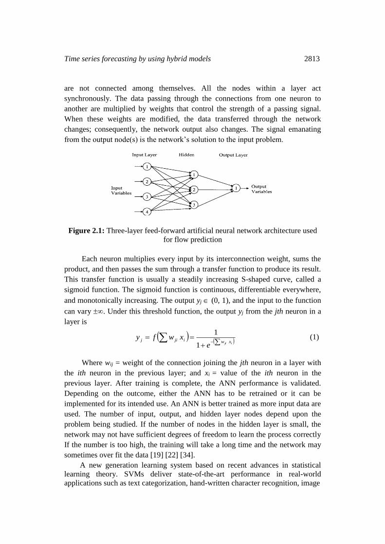
will be limited to only main concepts. A three layer, feed forward ANN is shown

in (Figure 2.1). It has input, output, and hidden middle layers. Each neuron in a

layer is connected to all the neurons of the next layer, and the neurons in one layer


are not connected among themselves. All the nodes within a layer act

synchronously. The data passing through the connections from one neuron to

another are multiplied by weights that control the strength of a passing signal.

When these weights are modified, the data transferred through the network

changes; consequently, the network output also changes. The signal emanating

from the output node(s) is the network’s solution to the input problem.

Figure 2.1: Three-layer feed-forward artificial neural network architecture used

for flow prediction

Each neuron multiplies every input by its interconnection weight, sums the

product, and then passes the sum through a transfer function to produce its result.

This transfer function is usually a steadily increasing S-shaped curve, called a

sigmoid function. The sigmoid function is continuous, differentiable everywhere,

and monotonically increasing. The output yj (0, 1), and the input to the function

can vary . Under this threshold function, the output yj from the jth neuron in a

layer is

iji xwijij

exwfy

1

1 (1)

Where wij = weight of the connection joining the jth neuron in a layer with

the ith neuron in the previous layer; and xi = value of the ith neuron in the

previous layer. After training is complete, the ANN performance is validated.

Depending on the outcome, either the ANN has to be retrained or it can be

implemented for its intended use. An ANN is better trained as more input data are

used. The number of input, output, and hidden layer nodes depend upon the

problem being studied. If the number of nodes in the hidden layer is small, the

network may not have sufficient degrees of freedom to learn the process correctly

If the number is too high, the training will take a long time and the network may

sometimes over fit the data [19] [22] [34].

A new generation learning system based on recent advances in statistical

learning theory. SVMs deliver state-of-the-art performance in real-world

applications such as text categorization, hand-written character recognition, image


classification, bio-sequences analysis, river flow and traffic flow forecast etc., and

are now established as one of the standard tools for machine learning and data

mining. Support vector machines (SVMs) appeared in the early nineties as

optimal margin classifiers in the context of Vapnik’s statistical learning theory.

Since then SVMs have been successfully applied to real-world data analysis

problems, often providing improved results compared with other techniques.

2.2 Least Square Support Vector Machines (LSSVM) Model

LSSVM optimizes SVM by replacing complex quadratic programming. It

achieves this by using least squares loss function and equality constraints. For the

purpose of understanding about the construction of the model consider a training

sample set represented by ),( ii yx where xi represents the input training vector.

Suppose that this training vector belongs to ‘n’ dimensional space i.e. Rn, so we

can write n

i Rx . Similarly, suppose that yi represents the output and this output

can be described as, Ryi . SVM can be described with the help of Equation (2)

bxwxy T )()( (2)

Where )(x is a function that ensures the mapping of nonlinear values into

higher dimensional space. LSSVM formulates the regression problem according

to Equation (3)

n

i

i

T ewwewR1

2

22

1),(min

(3)

The regression model shown in Equation (2) works under the influence of

equality constraints

ii

T ebxwxy )()( , ni ...,,2,1 (4)

It introduces Lagrange multiplier for:

})({22

1),,,(

11

2

iii

Tn

i

i

n

i

i

T yebxwewwebwL

(5)

Where i represents Lagrange multipliers. Since Equation (5) involves

more than one variable so, for studying the rate of change partial differentiation of

Equation (6-9) is required. Therefore differentiating Equation (5) with respect to

iebw ,, and i and equating them equal to zero yields the following set of

Equations.

n

i

ii xww

L

1

)(0 (6)


n

i

ib

L

1

00 (7)

ii

i

ee

L

0 (8)

0)(0

iii

T

i

yebxwL

, ni ...,,2,1 (9)

Substituting Equation (6-8) in Equation (5) we get the value of ‘w’. This ‘w’ is

described according to Equation (19)

n

i

ii

n

i

ii xexw11

)()( (10)

Putting Equation (10) in Equation (4)

bxxKbxxxyn

i

ii

n

i

i

T

ii 11

),()()()( (11)

Where, K(xi, x), represents a kernel such that:

)()(),( i

T

ii xxxxK

(12)

The vector which is a Lagrange Multiplier and the Biased can be computed by

solving a set of linear equations shown in Equation (13)

y

b

Ixx j

T

i

T0

)()(

01 1

1

(13)

Where, nyyy ...;;1 , 1...;;11 , n ...;;1 . This eventually constitutes

LSSVM model which is described according to Equation (14).

bxxKxyn

i

ii 1

),()( (14)

The model shown in Equation (14) deals with the linear system and

solution this linear system is provided by i , b . The high dimensional feature

space is defined by a function. This function is generally known as ‘kernel

function’ and is represented by ),( xxK i There are various choices available for

picking up this function.

2.3 Discrete Wavelet Transform (DWT)

Wavelets are becoming an increasingly important tool in time series

forecasting. The basic objective of wavelet transformation is to analyze the time

series data both in the time and frequency domain by decomposing the original time series in different frequency bands using wavelet functions. Unlike the Fourier


transform, in which time series are analyzed using sine and cosine functions,

wavelet transformations provide useful decomposition of original time series by

capturing useful information on various decomposition levels.

Assuming a continuous time series )(tx , ],[ t , a wavelet function can

be written as

s

t

sst

1),( (15)

where t stands for time, for the time step in which the window function is

iterated, and ],0[ s for the wavelet scale. )(t called the mother wavelet can

be defined as 0)(

dtt . The continuous wavelet transform (CWT) is given

by

dts

ttx

ssW

)(

1),( (16)

where )(t stands for the complex conjugation of )(t . ),( sW presents the

sum over all time of the time series multiplied by scale and shifted version of

wavelet function )(t . The use of continuous wavelet transform for forecasting

is not practically possible because calculating wavelet coefficient at every

possible scale is time consuming and it generates a lot of data.

Therefore, Discrete Wavelet Transformation (DWT) is preferred in most

of the forecasting problems because of its simplicity and ability to compute with

less time. The DWT involves choosing scales and position on powers of 2,

so-called dyadic scales and translations, then the analysis will be much more

efficient as well as more accurate. The main advantage of using the DWT is its

robustness as it does not include any potentially erroneous assumption or

parametric testing procedure [24][9][31]. The DWT can be defined as

m

m

mnm

s

snt

ss

t

0

00

2/

0

,

1

(17)

Where, m and n are integers that control the scale and time, respectively; 0s

is a specified, fixed dilation step greater than 1; and 0 is the location parameter,

which must be greater than zero. The most common choices for the parameters

0s = 2 and 0 = 1. For a discrete time series )(tx where )(tx occurs at discrete

time t, the DWT becomes

1

0

2/

, )()2(2N

t

mm

nm txntW (18)

Where, nmW , is the wavelet coefficient for the discrete wavelet at scale ms 2 and nm2 . In Eq. (18), )(tx is time series (t = 1, 2, …, N-1), and N is


an integer to the power of 2 (N= 2M); n is the time translation parameter, which

changes in the ranges 0 < n < 2M – m, where 1 < m < M.

According to Mallat’s theory [1], the original discrete time series )(tx can be

decomposed into a series of linearity independent approximation and detail

signals by using the inverse DWT. The inverse DWT is given by [11] [24] [31].

M

m t

mm

nm

mM

ntWTtx1

2

0

2/

,

1

)2(2)( (19)

or in a simple format as

M

m

mM tDtAtx1

)()()( (20)

which )(tAM is called approximation sub-series or residual term at levels M

and )(tDm ( m = 1, 2, ..., M) are detail sub-series which can capture small features

of interpretational value in the data.

3 Application

In this study, the time series of monthly streamflow data of the Neelum

and Indus river of Pakistan are used. The Neelum River catchment covers an area

of 21359 km2 and the Indus River catchment covers 1165000 km2. The first set

of data comprises of monthly streamflow data of Neelum River from January

1983 to February 2012 and the second data of set of streamflow data of Indus

River January 1983 to March 2013. In the application, the first 75% of the whole

data set were used for training the network to obtain the parameters model.

Another 20% of the whole dataset was used for testing. The comprehensive assessments of model performance atleast mean

absolute error (MAE) measures, root mean square error (RMSE) and correlation

coefficient (R). Evaluated the results of time series forecasting data to check the

performance of all models for forecasting data and training data.

n

t

tt yyn

MAE1

ˆ1

(21)

n

t

tt yyn

RMSE1

ˆ1

(22)

)23(

ˆˆ11

ˆ1

2

1

2

1

1

n

t

t

n

t

t

tt

n

t

t

yyn

yyn

yyyyn

R

Where n is the number of observation, ty

stands for the forecasting rainfall, yt is

the observed rainfall at all-time t.


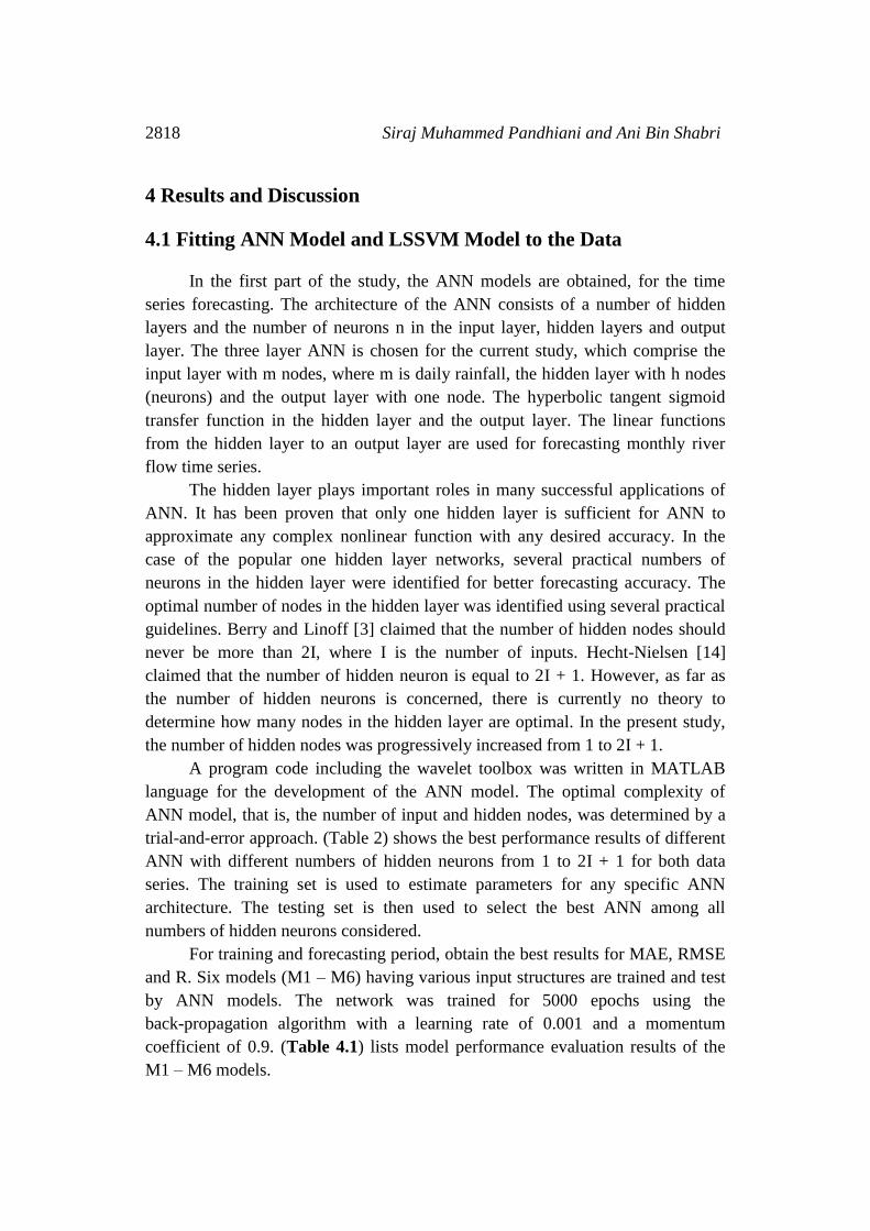
4 Results and Discussion

4.1 Fitting ANN Model and LSSVM Model to the Data

In the first part of the study, the ANN models are obtained, for the time

series forecasting. The architecture of the ANN consists of a number of hidden

layers and the number of neurons n in the input layer, hidden layers and output

layer. The three layer ANN is chosen for the current study, which comprise the

input layer with m nodes, where m is daily rainfall, the hidden layer with h nodes

(neurons) and the output layer with one node. The hyperbolic tangent sigmoid

transfer function in the hidden layer and the output layer. The linear functions

from the hidden layer to an output layer are used for forecasting monthly river

flow time series.

The hidden layer plays important roles in many successful applications of

ANN. It has been proven that only one hidden layer is sufficient for ANN to

approximate any complex nonlinear function with any desired accuracy. In the

case of the popular one hidden layer networks, several practical numbers of

neurons in the hidden layer were identified for better forecasting accuracy. The

optimal number of nodes in the hidden layer was identified using several practical

guidelines. Berry and Linoff [3] claimed that the number of hidden nodes should

never be more than 2I, where I is the number of inputs. Hecht-Nielsen [14]

claimed that the number of hidden neuron is equal to 2I + 1. However, as far as

the number of hidden neurons is concerned, there is currently no theory to

determine how many nodes in the hidden layer are optimal. In the present study,

the number of hidden nodes was progressively increased from 1 to 2I + 1.

A program code including the wavelet toolbox was written in MATLAB

language for the development of the ANN model. The optimal complexity of

ANN model, that is, the number of input and hidden nodes, was determined by a

trial-and-error approach. (Table 2) shows the best performance results of different

ANN with different numbers of hidden neurons from 1 to 2I + 1 for both data

series. The training set is used to estimate parameters for any specific ANN

architecture. The testing set is then used to select the best ANN among all

numbers of hidden neurons considered.

For training and forecasting period, obtain the best results for MAE, RMSE

and R. Six models (M1 – M6) having various input structures are trained and test

by ANN models. The network was trained for 5000 epochs using the

back-propagation algorithm with a learning rate of 0.001 and a momentum

coefficient of 0.9. (Table 4.1) lists model performance evaluation results of the

M1 – M6 models.


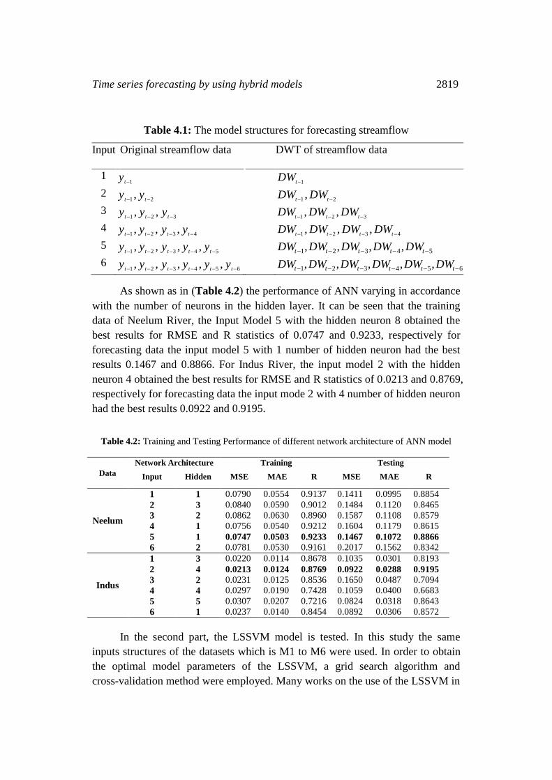
Table 4.1: The model structures for forecasting streamflow

Input Original streamflow data DWT of streamflow data

1 1t

y

1t

DW

2 21

, tt

yy

21

, tt

DWDW

3 321

,, ttt

yyy

321

,, ttt

DWDWDW

4 4321

,,, tttt

yyyy

4321

,,, tttt

DWDWDWDW

5 54321

,,,, ttttt

yyyyy

54321 ,,,, ttttt DWDWDWDWDW

6 654321

,,,,, tttttt

yyyyyy

654321 ,,,,, tttttt DWDWDWDWDWDW

As shown as in (Table 4.2) the performance of ANN varying in accordance

with the number of neurons in the hidden layer. It can be seen that the training

data of Neelum River, the Input Model 5 with the hidden neuron 8 obtained the

best results for RMSE and R statistics of 0.0747 and 0.9233, respectively for

forecasting data the input model 5 with 1 number of hidden neuron had the best

results 0.1467 and 0.8866. For Indus River, the input model 2 with the hidden

neuron 4 obtained the best results for RMSE and R statistics of 0.0213 and 0.8769,

respectively for forecasting data the input mode 2 with 4 number of hidden neuron

had the best results 0.0922 and 0.9195.

Table 4.2: Training and Testing Performance of different network architecture of ANN model

Data

Network Architecture Training Testing

Input Hidden MSE MAE R MSE MAE R

Neelum

1 1 0.0790 0.0554 0.9137 0.1411 0.0995 0.8854

2 3 0.0840 0.0590 0.9012 0.1484 0.1120 0.8465

3 2 0.0862 0.0630 0.8960 0.1587 0.1108 0.8579

4 1 0.0756 0.0540 0.9212 0.1604 0.1179 0.8615

5 1 0.0747 0.0503 0.9233 0.1467 0.1072 0.8866

6 2 0.0781 0.0530 0.9161 0.2017 0.1562 0.8342

Indus

1 3 0.0220 0.0114 0.8678 0.1035 0.0301 0.8193

2 4 0.0213 0.0124 0.8769 0.0922 0.0288 0.9195

3 2 0.0231 0.0125 0.8536 0.1650 0.0487 0.7094

4 4 0.0297 0.0190 0.7428 0.1059 0.0400 0.6683

5 5 0.0307 0.0207 0.7216 0.0824 0.0318 0.8643

6 1 0.0237 0.0140 0.8454 0.0892 0.0306 0.8572

In the second part, the LSSVM model is tested. In this study the same

inputs structures of the datasets which is M1 to M6 were used. In order to obtain

the optimal model parameters of the LSSVM, a grid search algorithm and

cross-validation method were employed. Many works on the use of the LSSVM in


time series modeling and forecasting have demonstrated favorable performances

of the RBF [41][28]. Therefore, RBF is used as the kernel function for

streamflow forecasting in this study. The LSSVM model used herein has two

parameters (, 2) to be determined. The grid search method is a common method

which was applied to calibrate these parameters more effectively and

systematically to overcome the potential shortcomings of the trails and error

method. It is a straightforward and exhaustive method to search parameters. In

this study, a grid search of (, 2) with in the range 10 to 1000 and 2 in the

range 0.01 to 1.0 was conducted to find the optimal parameters. In order to avoid

the danger of over fitting, the cross-validation scheme is used to calibrate the

parameters. For each hyper parameter pair (, 2) in the search space, 10-fold

cross validation on the training set was performed to predict the prediction error.

The best fit model structure for each model is determined according to the criteria

of the performance evaluation.

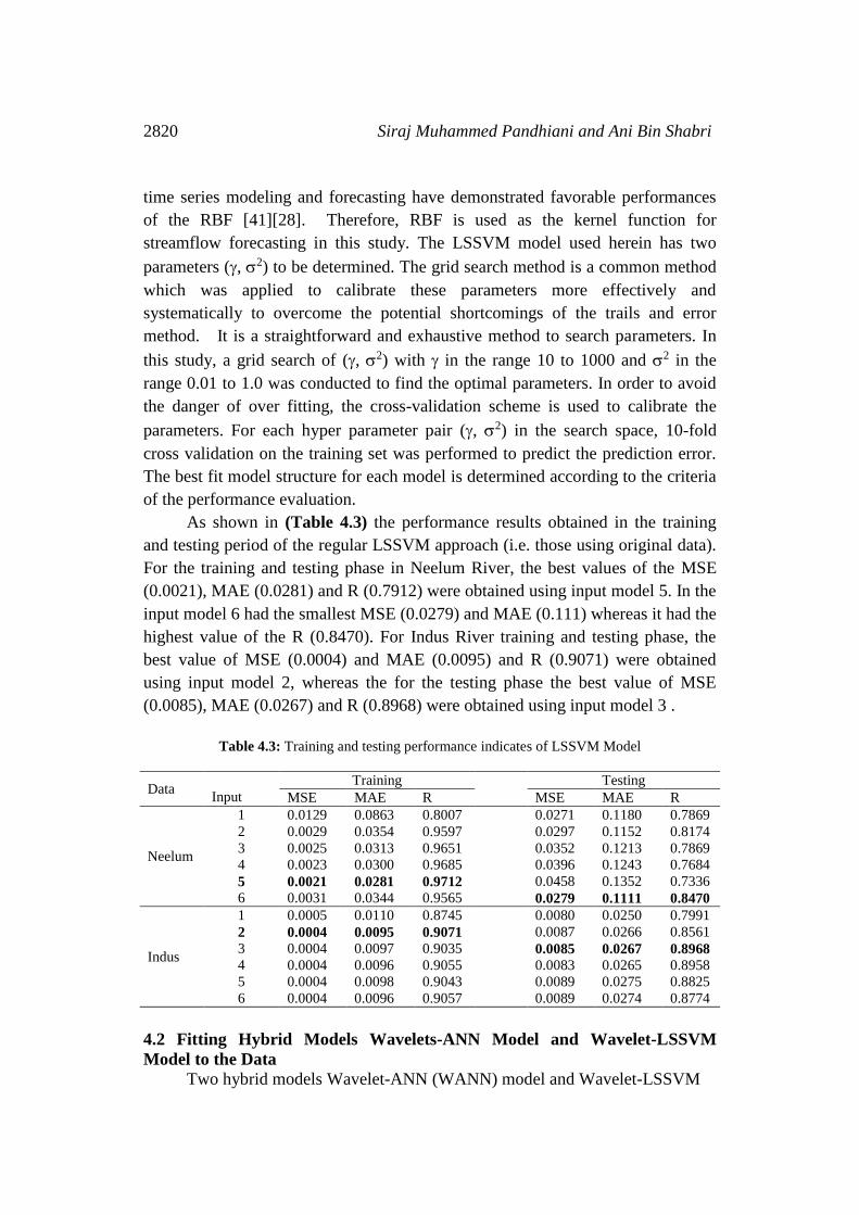
As shown in (Table 4.3) the performance results obtained in the training

and testing period of the regular LSSVM approach (i.e. those using original data).

For the training and testing phase in Neelum River, the best values of the MSE

(0.0021), MAE (0.0281) and R (0.7912) were obtained using input model 5. In the

input model 6 had the smallest MSE (0.0279) and MAE (0.111) whereas it had the

highest value of the R (0.8470). For Indus River training and testing phase, the

best value of MSE (0.0004) and MAE (0.0095) and R (0.9071) were obtained

using input model 2, whereas the for the testing phase the best value of MSE

(0.0085), MAE (0.0267) and R (0.8968) were obtained using input model 3 .

Table 4.3: Training and testing performance indicates of LSSVM Model

Data

Input

Training Testing

MSE MAE R MSE MAE R

Neelum

1 0.0129 0.0863 0.8007 0.0271 0.1180 0.7869

2 0.0029 0.0354 0.9597 0.0297 0.1152 0.8174

3 0.0025 0.0313 0.9651 0.0352 0.1213 0.7869

4 0.0023 0.0300 0.9685 0.0396 0.1243 0.7684

5 0.0021 0.0281 0.9712 0.0458 0.1352 0.7336

6 0.0031 0.0344 0.9565 0.0279 0.1111 0.8470

Indus

1 0.0005 0.0110 0.8745 0.0080 0.0250 0.7991

2 0.0004 0.0095 0.9071 0.0087 0.0266 0.8561

3 0.0004 0.0097 0.9035 0.0085 0.0267 0.8968

4 0.0004 0.0096 0.9055 0.0083 0.0265 0.8958

5 0.0004 0.0098 0.9043 0.0089 0.0275 0.8825

6 0.0004 0.0096 0.9057 0.0089 0.0274 0.8774

4.2 Fitting Hybrid Models Wavelets-ANN Model and Wavelet-LSSVM

Model to the Data

Two hybrid models Wavelet-ANN (WANN) model and Wavelet-LSSVM


(WLSSVM) model are obtained by combining two methods, discrete transform

(DWT) and ANN model and discrete transform (DWT) and LSSVM. In WANN

and WLSSVM, the original time series was decomposed into a certain number of

sub-time series components which were entered ANN and LSSVM in order to

improve the model accuracy. In this study, the Deubechies wavelet, one of the

most widely used wavelet families, is chosen as the wavelet function to

decompose the original series [11] [24] [31] [32]. The observed series was

decomposed into a number of wavelet components, depending on the selected

decomposition levels. Deciding the optimal decomposition level of the time series

data in wavelet analysis plays an important role in preserving the information and

reducing the distortion of the datasets. However, there is no existing theory to tell

how many decomposition levels are needed for any time series. To select the

number of decomposition levels, the following formula is used to determine the

decomposition level [24] [32] M = log (n).

Where, n is length of the time series and M is decomposition level. In this

study, n = 350 and n = 483 monthly data are used for Neelum and Indus,

respectively, which approximately gives M = 3 decomposition levels. Three

decomposition levels are employed in this study, the same as studies employed by

[30]. The observed time series of discharge flow data was decomposed at 3

decomposition levels (2 – 4 – 8 months).

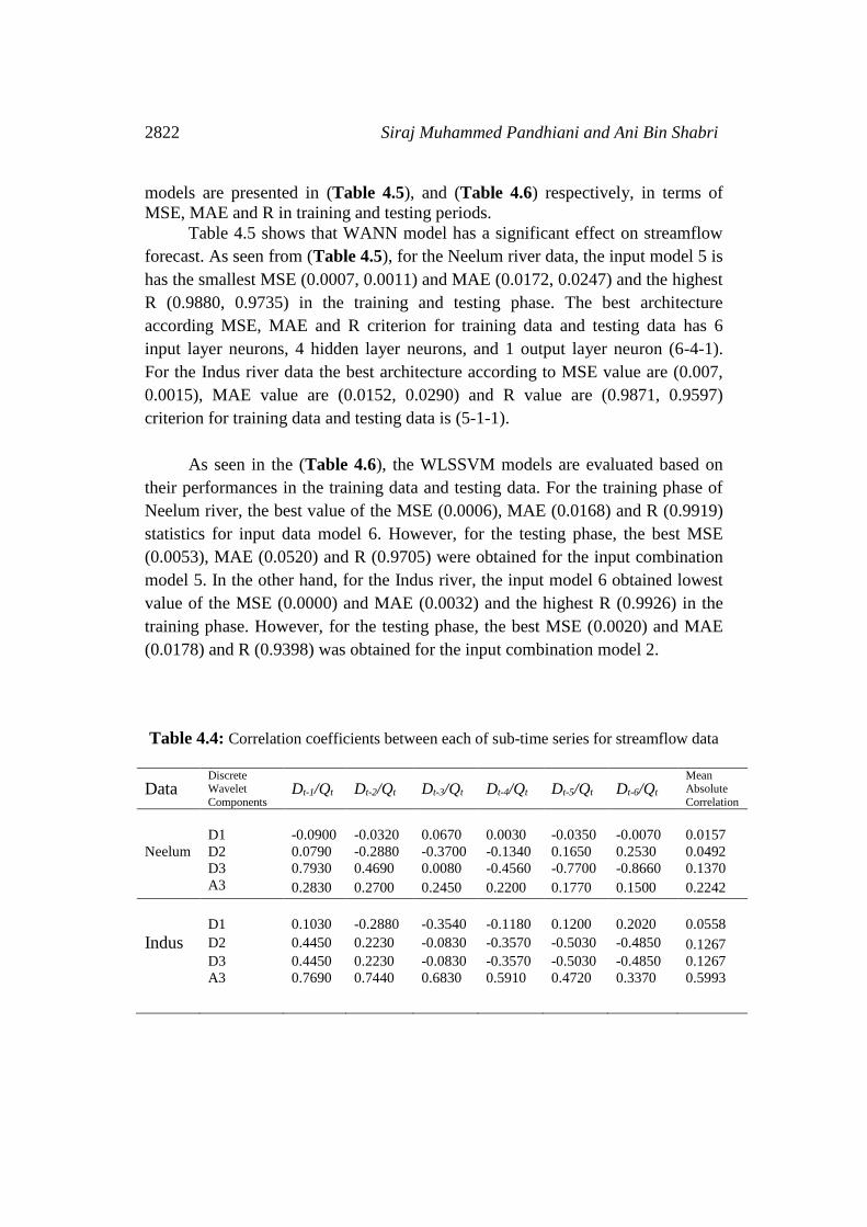
The effectiveness of wavelet components is determined using the

correlation between the observed streamflow data and the wavelet coefficients of

different decomposition levels. (Table 4.4) shows the correlations between each

wavelet component time series and original monthly stream flow data. It is

observed that the D1 component shows low correlations. The correlation

between the wavelet component D2 and D3 of the monthly stream flow and the

observed monthly stream flow data show significantly higher correlations

compared to the D1 components. Afterward, the significant wavelet components

D2, D3 and approximation (A3) component were added to each other to constitute

the new series. For the WANN model and WLSSVM model, the new series is

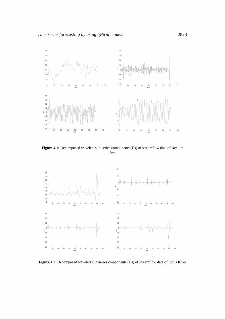
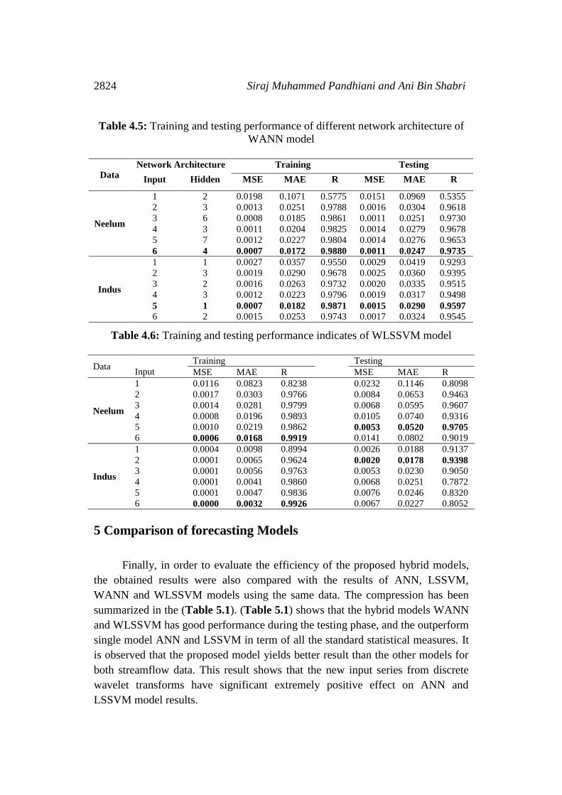
used as inputs to the ANN and LSSVM model. (Figure 4.1) and (Figure 4.2)

shows the original streamflow data time and their Ds, that is the time series of

2-month mode (D1), 4-month mode (D2) , 8-month mode (D3), approximate

mode (A3), and the combinations of effective details and approximation

components mode ( A2 + D2 + D3). Six different combinations of the new

series input data (Table 4.1) is used for forecasting as in the previous application.

A program code including wavelet toolbox was written in MATLAB

language for the development of ANN and LSSVM. The forecasting

performances of the Wavelet-ANN (WANN) and Wavelet-LSSVM (WLSSVM)


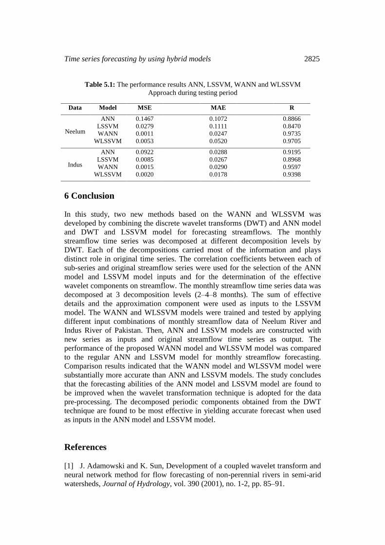
models are presented in (Table 4.5), and (Table 4.6) respectively, in terms of

MSE, MAE and R in training and testing periods.

Table 4.5 shows that WANN model has a significant effect on streamflow

forecast. As seen from (Table 4.5), for the Neelum river data, the input model 5 is

has the smallest MSE (0.0007, 0.0011) and MAE (0.0172, 0.0247) and the highest

R (0.9880, 0.9735) in the training and testing phase. The best architecture

according MSE, MAE and R criterion for training data and testing data has 6

input layer neurons, 4 hidden layer neurons, and 1 output layer neuron (6-4-1).

For the Indus river data the best architecture according to MSE value are (0.007,

0.0015), MAE value are (0.0152, 0.0290) and R value are (0.9871, 0.9597)

criterion for training data and testing data is (5-1-1).

As seen in the (Table 4.6), the WLSSVM models are evaluated based on

their performances in the training data and testing data. For the training phase of

Neelum river, the best value of the MSE (0.0006), MAE (0.0168) and R (0.9919)

statistics for input data model 6. However, for the testing phase, the best MSE

(0.0053), MAE (0.0520) and R (0.9705) were obtained for the input combination

model 5. In the other hand, for the Indus river, the input model 6 obtained lowest

value of the MSE (0.0000) and MAE (0.0032) and the highest R (0.9926) in the

training phase. However, for the testing phase, the best MSE (0.0020) and MAE

(0.0178) and R (0.9398) was obtained for the input combination model 2.

Table 4.4: Correlation coefficients between each of sub-time series for streamflow data

Data

Discrete Wavelet

Components Dt-1/Qt Dt-2/Qt Dt-3/Qt Dt-4/Qt Dt-5/Qt Dt-6/Qt

Mean Absolute

Correlation

D1 -0.0900 -0.0320 0.0670 0.0030 -0.0350 -0.0070 0.0157

Neelum D2 0.0790 -0.2880 -0.3700 -0.1340 0.1650 0.2530 0.0492

D3 0.7930 0.4690 0.0080 -0.4560 -0.7700 -0.8660 0.1370 A3 0.2830 0.2700 0.2450 0.2200 0.1770 0.1500 0.2242

D1

0.1030

-0.2880

-0.3540

-0.1180

0.1200

0.2020 0.0558

Indus D2 0.4450 0.2230 -0.0830 -0.3570 -0.5030 -0.4850 0.1267 D3 0.4450 0.2230 -0.0830 -0.3570 -0.5030 -0.4850 0.1267 A3 0.7690 0.7440 0.6830 0.5910 0.4720 0.3370 0.5993


0 50 100 150 200 250 300 350 400

0.2

0.25

0.3

0.35

0.4

0.45

0.5

Months

A3

-a

pp

ro

xim

atio

n

0 50 100 150 200 250 300 350 400-0.15

-0.1

-0.05

0

0.05

0.1

0.15

0.2

Months

D1

0 50 100 150 200 250 300 350 400-0.2

-0.15

-0.1

-0.05

0

0.05

0.1

0.15

0.2

Months

D2

0 50 100 150 200 250 300 350 400-0.4

-0.3

-0.2

-0.1

0

0.1

0.2

0.3

Months

D3

Figure 4.1: Decomposed wavelets sub-series components (Ds) of streamflow data of Neelum

River

0 50 100 150 200 250 300 350 400 450 5000

0.05

0.1

0.15

0.2

0.25

0.3

0.35

0.4

Months

A3

-a

pp

ro

xim

atio

n

0 50 100 150 200 250 300 350 400 450 500-0.15

-0.1

-0.05

0

0.05

0.1

Months

D1

0 50 100 150 200 250 300 350 400 450 500-0.4

-0.3

-0.2

-0.1

0

0.1

0.2

0.3

Months

D2

0 50 100 150 200 250 300 350 400 450 500-0.4

-0.3

-0.2

-0.1

0

0.1

0.2

0.3

Months

D3

Figure 4.2: Decomposed wavelets sub-series components (Ds) of streamflow data of Indus River


Table 4.5: Training and testing performance of different network architecture of

WANN model

Data Network Architecture Training Testing

Input Hidden MSE MAE R MSE MAE R

Neelum

1 2 0.0198 0.1071 0.5775 0.0151 0.0969 0.5355

2 3 0.0013 0.0251 0.9788 0.0016 0.0304 0.9618

3 6 0.0008 0.0185 0.9861 0.0011 0.0251 0.9730

4 3 0.0011 0.0204 0.9825 0.0014 0.0279 0.9678

5 7 0.0012 0.0227 0.9804 0.0014 0.0276 0.9653

6 4 0.0007 0.0172 0.9880 0.0011 0.0247 0.9735

Indus

1 1 0.0027 0.0357 0.9550 0.0029 0.0419 0.9293

2 3 0.0019 0.0290 0.9678 0.0025 0.0360 0.9395

3 2 0.0016 0.0263 0.9732 0.0020 0.0335 0.9515

4 3 0.0012 0.0223 0.9796 0.0019 0.0317 0.9498

5 1 0.0007 0.0182 0.9871 0.0015 0.0290 0.9597

6 2 0.0015 0.0253 0.9743 0.0017 0.0324 0.9545

Table 4.6: Training and testing performance indicates of WLSSVM model

Data

Input

Training Testing

MSE MAE R MSE MAE R

Neelum

1 0.0116 0.0823 0.8238 0.0232 0.1146 0.8098

2 0.0017 0.0303 0.9766 0.0084 0.0653 0.9463

3 0.0014 0.0281 0.9799 0.0068 0.0595 0.9607

4 0.0008 0.0196 0.9893 0.0105 0.0740 0.9316

5 0.0010 0.0219 0.9862 0.0053 0.0520 0.9705

6 0.0006 0.0168 0.9919 0.0141 0.0802 0.9019

Indus

1 0.0004 0.0098 0.8994 0.0026 0.0188 0.9137

2 0.0001 0.0065 0.9624 0.0020 0.0178 0.9398

3 0.0001 0.0056 0.9763 0.0053 0.0230 0.9050

4 0.0001 0.0041 0.9860 0.0068 0.0251 0.7872

5 0.0001 0.0047 0.9836 0.0076 0.0246 0.8320

6 0.0000 0.0032 0.9926 0.0067 0.0227 0.8052

5 Comparison of forecasting Models

Finally, in order to evaluate the efficiency of the proposed hybrid models,

the obtained results were also compared with the results of ANN, LSSVM,

WANN and WLSSVM models using the same data. The compression has been

summarized in the (Table 5.1). (Table 5.1) shows that the hybrid models WANN

and WLSSVM has good performance during the testing phase, and the outperform

single model ANN and LSSVM in term of all the standard statistical measures. It

is observed that the proposed model yields better result than the other models for

both streamflow data. This result shows that the new input series from discrete

wavelet transforms have significant extremely positive effect on ANN and

LSSVM model results.


Table 5.1: The performance results ANN, LSSVM, WANN and WLSSVM

Approach during testing period

Data Model MSE MAE R

Neelum

ANN 0.1467 0.1072 0.8866

LSSVM 0.0279 0.1111 0.8470

WANN 0.0011 0.0247 0.9735

WLSSVM 0.0053 0.0520 0.9705

Indus

ANN 0.0922 0.0288 0.9195

LSSVM 0.0085 0.0267 0.8968

WANN 0.0015 0.0290 0.9597

WLSSVM 0.0020 0.0178 0.9398

6 Conclusion

In this study, two new methods based on the WANN and WLSSVM was

developed by combining the discrete wavelet transforms (DWT) and ANN model

and DWT and LSSVM model for forecasting streamflows. The monthly

streamflow time series was decomposed at different decomposition levels by

DWT. Each of the decompositions carried most of the information and plays

distinct role in original time series. The correlation coefficients between each of

sub-series and original streamflow series were used for the selection of the ANN

model and LSSVM model inputs and for the determination of the effective

wavelet components on streamflow. The monthly streamflow time series data was

decomposed at 3 decomposition levels (2–4–8 months). The sum of effective

details and the approximation component were used as inputs to the LSSVM

model. The WANN and WLSSVM models were trained and tested by applying

different input combinations of monthly streamflow data of Neelum River and

Indus River of Pakistan. Then, ANN and LSSVM models are constructed with

new series as inputs and original streamflow time series as output. The

performance of the proposed WANN model and WLSSVM model was compared

to the regular ANN and LSSVM model for monthly streamflow forecasting.

Comparison results indicated that the WANN model and WLSSVM model were

substantially more accurate than ANN and LSSVM models. The study concludes

that the forecasting abilities of the ANN model and LSSVM model are found to

be improved when the wavelet transformation technique is adopted for the data

pre-processing. The decomposed periodic components obtained from the DWT

technique are found to be most effective in yielding accurate forecast when used

as inputs in the ANN model and LSSVM model.

References

[1] J. Adamowski and K. Sun, Development of a coupled wavelet transform and

neural network method for flow forecasting of non-perennial rivers in semi-arid

watersheds, Journal of Hydrology, vol. 390 (2001), no. 1-2, pp. 85–91.


http://dx.doi.org/10.1016/j.jhydrol.2010.06.033

[2] Asefa, T., Kemblowski, M., McKee, M., and Khalil, A., Multi-time scale

stream flow predictions: The support vector machines approach, J. Hydrol., 318

(1–4), (2006) 7–16. http://dx.doi.org/10.1016/j.jhydrol.2005.06.001

[3] M. J. A. Berry and G. S. Linoff, Data Mining Techniques: For Marketing,

Sales, and Customer Support, John Wiley & Sons, New York NY, USA, (1997).

[4] Bose, G. E. P., and Jenkins, G. M. Time series analysis forecasting and

control, Holden Day, San Francisco, (1970).

[5] I. Daubechies, Orthogonal bases of compactly supported wavelets, Commun.

Pure Applied Math., 41 (1988): 909-996.

http://dx.doi.org/10.1002/cpa.3160410705

[6] Delleur, J. W., Tao, P. C., and Kavvas, M., An evaluation of the practicality

and complexity of some rainfall and runoff time series model. Water resour. res.,

12(5) (1976), 953–970. http://dx.doi.org/10.1029/wr012i005p00953

[7] Dibike, Y. B., Velickov, S., Solomatine, D. P., and Abbott, M. B., Model

induction with support vector machines: introduction and applications, ASCE J.

Comput. Civil Eng., 15(3) (2001), 208–216.

http://dx.doi.org/10.1061/(asce)0887-3801(2001)15:3(208)

[8] Elshorbagy, A., Corzo, G., Srinivasulu, S., and Solomatine, D. P.

Experimental investigation of the predictive capabilities of data driven modeling

techniques in hydrology – Part 2: Application, Hydrol. Earth Syst. Sci. Discuss., 6

(2009), 7095–7142. http://dx.doi.org/10.5194/hessd-6-7095-2009

[9] M. Firat, Comparison of Artificial Intelligence Techniques for river flow

forecasting, Hydrol. Earth Syst. Sci., 12, 123–139 (2008).

http://dx.doi.org/10.5194/hess-12-123-2008

[10] Foufoula-Georgiou & P. E Kumar, Wavelets in Geophysics, ed. E.

Foufoula-Georgiou & P. Kumar, (San Diego and London: Academic), (1994).

[11] A. Grossman, and J. Morlet, Decomposition of Harley functions into square

integral wavelets of constant shape, SIAM J. Math.Anal. 15, (1984) pp. 723-736.

http://dx.doi.org/10.1137/0515056

[12] Hanbay, D. An expert system based on least square support vector machines

for diagnosis of valvular heart disease, Expert Syst. Appl., 36(4) (2009), 4232–

4238. http://dx.doi.org/10.1016/j.eswa.2008.04.010



http://dx.doi.org/10.1002/cpa.3160410705

http://dx.doi.org/10.1029/wr012i005p00953

http://dx.doi.org/10.1061/%28asce%290887-3801%282001%2915:3%28208%29

http://dx.doi.org/10.5194/hessd-6-7095-2009

http://dx.doi.org/10.5194/hess-12-123-2008

http://dx.doi.org/10.1137/0515056

http://dx.doi.org/10.1016/j.eswa.2008.04.010


[13] Haykin, S. Neural network, a comprehensive foundation, IEEE, New York,

(1994).

[14] Hecht-Nielsen, R. Neurocomputing, Addison-Wesley, New York, (1991).

[15] R. Hecht-Nielsen, Neurocomputing, Addison-Wesley, Reading, Mass, USA,

(1990).

[16] Hurst, H. E. Long term storage capacity of reservoirs. Trans. ASCE, 116

(1961), 770–799.

[17] S. Ismail, R. Samsuddin, and A. Shabri, A hybrid model of self organizing

maps and least square support vector machine. (2010), Hydrol. Earth Syst. Sci.

Discuss., Volume 7, 8179-8212. http://dx.doi.org/10.5194/hessd-7-8179-2010

[18] Kang, Y. W., Li, J., Cao, G. Y., Tu, H. Y., Li, J., and Yang, J., Dynamic

temperature modeling of an SOFC using least square support vector machines, J.

Power Sources, 179 (2008), 683–692.

http://dx.doi.org/10.1016/j.jpowsour.2008.01.022

[19] Karunanidhi, N., Grenney, J., Whitley, D., Bovee, K., Neural networks for

river flow prediction. J. Comp. in Civ. Engrg. 8 (2) (1994), 201–220.


[20] M. Khashei and M. Bijari, A novel hybridization of artificial neural networks

and ARIMA models for time series forecasting,” Applied Soft Computing Journal,

vol. 11, no. 2, pp. (2011), 2664–2675.

http://dx.doi.org/10.1016/j.asoc.2010.10.015

[21] Khashei, M. and Bijari, M. An artificial neural network (p,d,q) model for

time series forecasting, Expert Syst. Appl., 37 (2010), 479–489.


[22] Kisi, O., River flow modeling using artificial neural networks, (2004), J.

Hydrol. Eng., 9(1), 60–63.


[23] Kisi, O., Neural network and wavelet conjunction model for modelling

monthly level fluctuations in Turkey, Hydrological Processes, vol. 23, no. 14

(2009), pp. 2081–2092. http://dx.doi.org/10.1002/hyp.7340

[24] Kisi, O., Wavelet regression model for short-term streamflow forecasting. J.

Hydrol., 389 (2010): 344-353. http://dx.doi.org/10.1016/j.jhydrol.2010.06.013

[25] B. Krishna, Y. R. Satyaji Rao, P.C. Nayak, Time Series Modeling of River

http://dx.doi.org/10.5194/hessd-7-8179-2010

http://dx.doi.org/10.1016/j.jpowsour.2008.01.022


http://dx.doi.org/10.1016/j.asoc.2010.10.015



http://dx.doi.org/10.1002/hyp.7340



Flow Using Wavelet Neutral Networks, Journal of Water Resources and

Protection, 3 (2011), 50-59. http://dx.doi.org/10.4236/jwarp.2011.31006

[26] D. Labat, R. Ababou and A. Mangin, Rainfall-Runoff Relations for Karastic

Springs: Part II. Continuous Wavelet and Discrete Orthogonal Multiresolution

Analysis, Journal of Hydrology, Vol. 238, No.3–4 (2000), pp. 149–178.

http://dx.doi.org/10.1016/s0022-1694(00)00322-x

[27] Lin, J. Y., Cheng, C. T., and Chau, K. W. Using support vector machines for

long-term discharge prediction, Hydrology Sci. J., 51 (4) (2006), 599–612.

http://dx.doi.org/10.1623/hysj.51.4.599

[28] Liu, L. and Wang, W., Exchange rates forecasting with least squares support

vector machines, International Conference on Computer Science and Software

Engineering, (2008), 1017–1019.

http://dx.doi.org/10.1109/csse.2008.140

[29] S. G. Mallat, A theory for multi resolution signal decomposition: The

wavelet representation, IEEE Transactions on Pattern Analysis and Machine

Intelligence, 11(7) (1998): 674-693.

http://dx.doi.org/10.1109/34.192463

[30] Matalas, N. C., Mathematical assessment of symmetric hydrology. Water

Resour. Press, 3(4) (1967), 937–945.


[31] PY. Ma, A fresh engineering approach for the forecast of financial index

volatility and hedging strategies, PhD thesis, Quebec University, Montreal,

Canada, (2006).

[32] S. Pandhiani and A. Shabri, Time Series Forecasting Using Wavelet-Least

Squares Support Vector Machines and Wavelet Regression Models for Monthly

Stream Flow Data," Open Journal of Statistics, Vol. 3 No. 3 (2013), pp. 183-194.

http://dx.doi.org/10.4236/ojs.2013.33021

[33] R. M Rao, and A.S. Bopardikar, Wavelet Transforms: Introduction to Theory

and Applications, Addison Wesley Longman, Inc., (1998), 310 pp.

[34] Rumelhart, D. E., Hinton, G. E., and Williams, R. J., Learning internal

representation by error propagation, Parallel distributed processing. Volume

1(1986): Foundations, eds., MIT Press, Cambridge, Mass.

[35] LC. Simith, DL. Turcotte, B. Isacks, Streamflow characterization and feature

detection using a discrete wavelet transform, Hydrological processes 12(1998):

233-249.

http://dx.doi.org/10.4236/jwarp.2011.31006

http://dx.doi.org/10.1016/s0022-1694%2800%2900322-x

http://dx.doi.org/10.1623/hysj.51.4.599

http://dx.doi.org/10.1109/csse.2008.140

http://dx.doi.org/10.1109/34.192463


http://dx.doi.org/10.4236/ojs.2013.33021


http://dx.doi.org/10.1002/(sici)1099-1085(199802)12:2<233::aid-hyp573>3.0.co;

2-3

[36] Suykens, J. A. K., Vandewalle, J. Least squares support vector machine

classifiers. Neural Processing Letters, Volume 3 (1999), 293-300.

[37] Vapnik, V. The nature of Statistical Learning Theory, Springer Verlag,

Berlin, (1995). http://dx.doi.org/10.1007/978-1-4757-2440-0

[38] D. Wang and J. Ding, Wavelet network Model and Its Application to the

Prediction of Hydrology, Nature and Science, Vol. 1 (2003), pp.67-71.

[39] Wang, H. and Hu, D. Comparison of SVM and LS-SVM for Regression,

IEEE, (2005), 279–283. http://dx.doi.org/10.1109/icnnb.2005.1614615

[40] Wang, W. C., Chau, K. W., Cheng, C. T., and Qiu, L., A Comparison of

Performance of Several Artificial Intelligence Methods for Forecasting Monthly

Discharge Time Series, J. Hydrol., 374 (2009), 294–306.


[41] Yu, P. S., Chen, S. T., and Chang, I. F., Support vector regression for

real-time flood stage forecasting, J. Hydrol., 328 (3–4) (2006), 704–716.


Received: March 9, 2015; Published: April 12, 2015

http://dx.doi.org/10.1002/%28sici%291099-1085%28199802%2912:2%3C233::aid-hyp573%3E3.0.co;2-3

http://dx.doi.org/10.1002/%28sici%291099-1085%28199802%2912:2%3C233::aid-hyp573%3E3.0.co;2-3

http://dx.doi.org/10.1007/978-1-4757-2440-0

http://dx.doi.org/10.1109/icnnb.2005.1614615



time series forecasting by using hybrid models for monthly ... · time series forecasting by using...

Documents