Scuola Dottorale di Ateneo

Graduate School

Dottorato di ricerca

in Economia

Ciclo XXIV

Anno di discussione 2013

Three Essays on Cheap Talk

SETTORE SCIENTIFICO DISCIPLINARE DI AFFERENZA: SECS-P/01

Tesi di Dottorato di Arya Kumar Srustidhar Chand, matricola 955562

Coordinatore del Dottorato Tutore del Dottorando

Prof. Michele Bernasconi Prof. Sergio Currarini

The undersigned Arya Kumar Srustidhar Chand, in his quality of doctoral candidate for

a Ph.D. degree in Economics granted by the Universita Ca’ Foscari Venezia and the Scuola

Superiore di Economia attests that the research exposed in this dissertation is original and

that it has not been and it will not be used to pursue or attain any other academic degree of

any level at any other academic institution, be it foreign or Italian.

c© Arya Kumar Srustidhar Chand, 2013

All Rights Reserved

On the Lotus Feet of

PARAMA PREMAMAYA

SREE SREE THAKUR ANUKULCHANDRA

&

Dedicated to

my grandfather late Mr. ANTARYAMI CHAND

my parents Mrs. HIRAMANI CHAND, Mr. BENUDHAR CHAND

Acknowledgments

I wish to express sincere gratitude to my thesis advisor Professor Sergio Currarini for his

guidance, encouragement and help throughout. I am indebted to him for teaching me different

aspects of research. His deep insight, critical reasoning and vast experience have been sources

of inspiration for me during the research period.

I owe a lot to Professor Piero Gottardi for introducing me the subject of Cheap Talk

and for being kind and supportive. I have always looked up to him to achieve academic

excellence. I am grateful to Professor Dezsoe Szalay for his guidance on one chapter of my

thesis, teaching me various dimensions of research and spending his valuable time to read my

research and communicating his opinions to me. I am thankful to Professor Marco LiCalzi

for teaching me a wonderful course on Game Theory and for always being supportive and

encouraging. I thank Professor Enrica Croda for her encouragement and help throughout.

I thank Dr. Giovanni Ursino very much for the discussions and our joint work which has

contributed to this thesis.

I am indebted to Professor Agar Brugiavini, the former Director of the Graduate Program

for always being kind and helpful. I am thankful to Professor Michele Bernasconi, the current

Director of the Graduate Program for his encouragement and support.

I humbly acknowledge the fellowship and facilities provided by the Ca’ Foscari University

of Venice during my research work. I am very grateful to the secretary of the graduate

program, Ms. Lisa Negrello for her prompt help during my every need.

I am obliged to the esteemed teachers at the Ca’ Foscari University of Venice, the Univer-

sity of Paris 1, Pantheon-Sorbonne, the Bielefeld University and the Chennai Mathematical

Institute from whom I have learnt a lot during my academic career; I would like to specially

mention Prof. Massimo Warglien, Prof. Monica Billio, Prof. Walter Trockel, Prof. Volker

i

Boehm, Prof. Peter Zeiner, Prof. Jean-Marc Bonnisseau, Prof. Pascal Gourdel, Prof. G.

Rajasekaran, Prof. R. Jagannathan, Prof. H.S. Mani, Prof. C.S. Aravinda. I thank Sri

Srinibas Pradhan and Jayanarayan Dash for their teaching during my school days. I thank

Prof. R.K. Amit and Prof. Noemi Pace for their encouragement.

The research journey would not have been wonderful had there not been my batch mates

Breno, Caterina and Matija. I learnt a lot from them, shared with them all the experiences

of the graduate life. All my best wishes to them and their family members Lillian, Luciano,

Solange, Franco, Raffaele, little Valerio. Many thanks to Anna, Ender, Giulia, Luca, Marisa,

Mithun, Nicola, Sonia for the time together in the first year of the graduate program and

also with many of them afterwards. I thank other graduate colleagues for the time together:

Ayo, Animesh, Chen, Claudio, Dragana, Francesco, Liudmila, Lorenza, Lorenzo, Stefano,

Vincenzo. Special thanks to Elena, Laura, Luis, Martin, Siddharth, Vahid and Yuri for being

always supportive.

I thank Davide for housing me for two beautiful years, for his kindness and help. His

family was like my family in Venice and I thank Flavia and Fiorenzo for taking so much

care of me as their own son. My best wishes to Eva, Stefano, Emma, little Tito, Pasqualina,

Rudolpho, Adda, Claudio and Irene. A lot of gratitude goes to Niccolo’ and Sara for their

kindness. Thanks to the friends with whom I spent beautiful time in Venice and Bonn:

Ana, Andrea Ambroso, Caterina Sorato, Daniela, Dhanya, Erisa, Fabio Biscaro, Fabio Lima,

Giuseppe, Harsha, Kaleab, Manoj, Marina, Mario, Mathis, Mike, Mirco Fabris, Patricia,

Patrick Aime, Pau, Petra, Prasanna, Shpendi, Siddesh. Many thanks go to Aditya, Arindam,

Pradeep, Raghuram, Sudhanshu, Upananda, Vishal and Xuexue. Special thanks to Shuvra

for his friendship and help, to Iaroslav, Saurabh, Tapopriya and Utsav for so many beautiful

moments in Europe.

No amount of words are sufficient to describe the contribution of my family in my ca-

reer. I am immensely grateful to my parents for being my first teachers, for their constant

inspiration and affording me all the things to progress in my career. I would not have pro-

ceeded to go so far in my career had there not been the support and teaching of my eldest

brother Bedabrata. I am very thankful to my sisters Lopamudra, Sebashree and Subhashree;

brothers Debabrata and Pranab Prakash; and my cousin brother Ajaya for their care and

help throughout my career. I am thankful to my sister-in-laws Pranita and Sandhyarani and

ii

brother-in-laws Abhimanyu, Suryaprasad, Krushnachandra and their families for their care

and support. I express my gratitude to Bhramarabar Bagha, my uncles Damodar, Niranjan;

my aunts Kamala, Bimala, Kanchana and their families especially my cousins Bijay, Sanjay

and Pramod. I am grateful to my late grandparents for their encouragement and their mem-

ories will be always with me. My nieces Lucy, Guddu, Khusi, Emoon, Trisha, Ramaya and

Duggu have made the world so beautiful, joyful and all my affections are for them.

I offer my regards to my Ritwik Sankarshan Samal for his guidance and encouragement.

I am grateful to late Chandrasekhar Mohapatra and late Bikashranjan Bhowmik for their

blessings. I am thankful to Bijayabhusan Mishra, Bauribandhu Nanda, Ramesh Ch. Swain,

Lokanath Mohanty, Ishwar Ch. Sahoo, Bairagi Ch. Sahoo, Birabara Sahoo, Rajanikanta

Pani, Adhikari M. Dash, Radhagobinda Mohapatra, Ratnakar Swain (S.P.R.s), Ananda Ch.

Sahoo, Arjuna Sutar, Jayakrushna Khatua, Sasikanta Pani and S.K. Acharya.

I offer my regards to Dr. Binayak Mohapatra, Sri Sridhar Sundar Mishra and Sri Abhay

Kumar Parida of the Satsang for their guidance and inspiration. Finally, I offer my sincerest

gratitude and salutations at the holy feet of Sree Sree Baroma, Yugacharya Sree Sree Borda,

Pradhan Acharyadev Sree Sree Dada, Pujaneeya Sree Sree Babaida and the members of the

Thakur Family of the Satsang for their blessings towards the work and a blissful life.

iii

Contents

Acknowledgments i

Preface 1

1 Strategic Information Transmission with Budget Constraint 5

1.1 Introduction . . . . . . . . . . . . . . . . . . . . . . . . . . . . . . . . . . . . . 6

1.1.1 Related Literature . . . . . . . . . . . . . . . . . . . . . . . . . . . . . 7

1.2 Model with Two Farmers . . . . . . . . . . . . . . . . . . . . . . . . . . . . . 9

1.3 Strategic Communication . . . . . . . . . . . . . . . . . . . . . . . . . . . . . 17

1.3.1 No Fully Revealing Equilibrium . . . . . . . . . . . . . . . . . . . . . . 17

1.3.2 Interval Partition . . . . . . . . . . . . . . . . . . . . . . . . . . . . . . 18

1.4 Effect of Budget on Information Transmission . . . . . . . . . . . . . . . . . . 20

1.4.1 Equilibrium where One Farmer Reveals Fully . . . . . . . . . . . . . . 21

1.4.2 {2} × {2} Symmetric Equilibria . . . . . . . . . . . . . . . . . . . . . . 22

1.5 Equilibrium Selection . . . . . . . . . . . . . . . . . . . . . . . . . . . . . . . 24

1.6 Conclusion . . . . . . . . . . . . . . . . . . . . . . . . . . . . . . . . . . . . . 27

1.7 Appendix . . . . . . . . . . . . . . . . . . . . . . . . . . . . . . . . . . . . . . 29

2 Cheap Talk with Correlated Signals 41

2.1 Introduction . . . . . . . . . . . . . . . . . . . . . . . . . . . . . . . . . . . . . 41

v

2.2 Model with Two Players . . . . . . . . . . . . . . . . . . . . . . . . . . . . . . 44

2.2.1 Truth Telling Equilibrium . . . . . . . . . . . . . . . . . . . . . . . . . 46

2.2.2 Selecting Correlation . . . . . . . . . . . . . . . . . . . . . . . . . . . . 49

2.3 Model with n-Players . . . . . . . . . . . . . . . . . . . . . . . . . . . . . . . . 54

2.3.1 Truth Telling Equilibrium . . . . . . . . . . . . . . . . . . . . . . . . . 56

2.3.2 Selecting Correlation . . . . . . . . . . . . . . . . . . . . . . . . . . . . 62

2.4 Conclusion . . . . . . . . . . . . . . . . . . . . . . . . . . . . . . . . . . . . . 68

2.5 Appendix . . . . . . . . . . . . . . . . . . . . . . . . . . . . . . . . . . . . . . 68

3 Information Transmission under Leakage 73

3.1 Introduction . . . . . . . . . . . . . . . . . . . . . . . . . . . . . . . . . . . . . 74

3.2 Model of Information Leakage . . . . . . . . . . . . . . . . . . . . . . . . . . . 76

3.3 Truth Telling Equilibrium . . . . . . . . . . . . . . . . . . . . . . . . . . . . . 77

3.4 Leakage vs Non-leakage . . . . . . . . . . . . . . . . . . . . . . . . . . . . . . 80

3.4.1 A Fixed First-hand Receiver . . . . . . . . . . . . . . . . . . . . . . . 81

3.4.2 Randomly Selected First-hand Receiver . . . . . . . . . . . . . . . . . 85

3.5 Conclusion . . . . . . . . . . . . . . . . . . . . . . . . . . . . . . . . . . . . . 86

3.6 Appendix . . . . . . . . . . . . . . . . . . . . . . . . . . . . . . . . . . . . . . 86

Bibliography 89

vi

Preface

My thesis contains three essays that are based on strategic communication associated with

the Cheap Talk literature. The essays are independent of each other and they study three

different problems associated with Cheap Talk. Each essay (chapter) is modeled like a paper

which makes it convenient for the readers to go through. Moreover, one can follow any

chapter without going through the other chapters.

The first essay is a discussion of strategic communication that arises in the classical

resource allocation problem. The second essay focuses on Cheap Talk where the signals of

the senders and the receiver are correlated. The third essay explores the theme where a

sender while transmitting the information takes into account that the information may be

leaked by the receiver to third party.

1

DISCERN AND KNOW THE

INTENT OF A WORD

First try to discern

the intent of a word,

then its usage–

in what affair

and how it is used;

know

the intent and its element

by which it occurs

and follow in application;

thus,

know the implication and sense

and use it

with confidence.

— Sree Sree Thakur

(The Message, Vol-VIII, Page-90)

3

Chapter 1

Strategic Information Transmission

with Budget Constraint

Abstract: In this chapter1, I discuss strategic communication that arises during the alloca-

tion of a limited budget or resource, in the context of water allocation to two farmers by the

social planner. Each farmer’s need of water is bounded and only he knows about his exact

need of water. Each farmer asks privately for an amount of water to the social planner and

then the social planner allocates water to the farmers. The utility function of each farmer is

a quadratic loss utility function where more water than the need causes flood or less water

causes drought. The social planner is a utilitarian and her utility is the sum of the utilities of

the two farmers. In this framework, when the amount of water is limited, I show that there is

no equilibrium where both the farmers ask exactly their own need. I also show that a higher

amount of water gives higher ex-ante expected utilities to all the players by considering (1)

an equilibrium where only one farmer reports the true need, (2) a symmetric equilibrium

where each farmer partitions his needs into two intervals. I provide arguments in favor of the

existence of equilibria where the needs of each farmer is partitioned into infinite intervals.

I propose that a symmetric equilibrium with infinite intervals for each farmer is the best

1This work was undertaken while I was a visiting student at the Bonn Graduate School of Economics in

2009-2010. I am grateful to Dezsoe Szalay for the guidance and advice. I am thankful to Mark Le Quement,

Sergio Currarini and Piero Gottardi for helpful discussions and comments. I also thank seminar participants

at the Ca’Foscari University and QED Jamboree 2012, Copenhagen for their valuable suggestions; particularly

Vahid Mojtahed for suggesting the example.

5

equilibrium for the social planner.

JEL Code : C72, D82, D83

Keywords : Cheap Talk, Multiple Senders, Budget Constraint

1.1 Introduction

Many social and commercial organizations generally have different branches to deal with

different issues. The organization frequently faces the decision of how much of the budget

or the resource to allocate to each branch. As many organizations do not possess adequate

wealth to give the desired amount of each branch, an organization faces a task of efficiently

allocating its wealth to its branches which is the classical budget allocation problem. But

each branch may like to get its best choice without caring about the whole organization by

misreporting its desired need. This forms the basis of the Cheap Talk setting that I set to

discuss in this paper.

Consider the following example to understand more about the strategic communication

due to budget constraint. There is the social planner (she) who wants to allocate water to

two farmers (he), call them farmer 1 and farmer 2. The social planner corresponds to the

receiver and the farmers correspond to the senders in the Cheap Talk literature. The social

planner may not have sufficient amount of water and she faces with the problem of allocating

a limited amount of water between the farmers. Each farmer’s need of water is his private

knowledge. Each farmer has quadratic utility function because a higher water than the need

can cause flood or less water can cause drought. The utility of the social planner is the sum

of the utilities of both the farmers. If there were no budget constraint, each farmer would ask

for the exact amount he needs and the social planner allocates him the exact amount. But

faced with a budget constraint, the social planner may not allocate the required amount to

each farmer. She allocates to each farmer that maximizes her utility within the budget limit

and so each farmer gets a reduced amount. But then one farmer may not like to ask the exact

amount he needs and will like to ask a higher amount, given the other farmer is asking his

exact amount with the social planner believing both the farmers. So the preferences (biases)

of the players differ and this gives rise to strategic communication found in the Cheap Talk

6

literature. In my model, the biases depend on what amounts the farmers need and also the

bias depends on how much budget is available, if there is sufficient budget, then there is no

bias among players. In this paper, I analyze various features like structure of equilibrium,

role of budget, equilibrium selection when there is strategic communication due to budget

constraint.

Discussing about the findings in my model, first I show that with a budget constraint

there is no full revelation i.e. for each farmer there exist some needs where he would prefer to

ask for higher amount of water so that the allocation he receives is close to his need. Then I

show that we have interval partition like the Crawford and Sobel (1982) [7] (henceforth CS)

model which means in the equilibrium, each farmer asks for higher amount of water if his

need increases. I discuss the effect of budget on information transmission in terms of ex-ante

expected utility with two types of equilibria: in the first type of equilibrium, only one farmer

reveals fully and the other farmer partitions his state into CS intervals; in the second type

of equilibrium, each farmer partitions the state space into two CS intervals and I consider

symmetric equilibrium where the intervals for both the farmers are identical. I demonstrate

that higher budget facilitates more information transmission because if the budget constraint

is relaxed, it is more probable that a farmer receives his required amount and hence the less

he would like to deviate. Then I discuss about selecting the equilibrium, for different values

of budget, between the above two types of equilibria. I provide some arguments that there

may exist equilibrium with infinite intervals of both the farmers in our model, but they are

challenging to compute. I conjecture that the symmetric equilibrium with infinite intervals

is the best equilibrium for the social planner.

1.1.1 Related Literature

In the seminal paper Strategic Information Transmission by Crawford and Sobel (1982) [7]

(CS), the authors described a form of communication which is costless (Cheap Talk) between

an informed sender and an uninformed receiver regarding the state of the Nature where the

players prefer different actions for given states of the Nature. The difference in preferences

between the players (in other words the difference in biases) given the states of the Nature

gives rise to strategic communication among players. Since then there have been numerous

papers on different aspects of Cheap Talk. Gilligan and Krehbiel(1989)[11], Krishna and

7

Morgan (2001) [16] are the main works with multiple senders in one-dimensional state space.

The paper of Krishna and Morgan [16] also discusses about the sequential communication.

Farrel and Gibbons (1989)[8] and Newmann and Sansing (1993)[21], Goltsman and Pavlov

(2011) [12] discuss Cheap Talk with multiple receivers. Battaglini (2002)[6], Levy and Razin

(2004)[22] are some of the works on Cheap Talk in multiple dimensions state and policy space.

Li (2003)[17] and Frisell and Lagerloef (2007)[9] discuss the Cheap Talk with uncertain biases.

The papers by Melumad and Shibano (1991) [19], Alonso et al. (2008)[2], Gordon (2010)[13]

discuss Cheap Talk where biases are state dependent.

My model incorporates many features of the above literature. In my model, I have

multiple senders with one receiver and I have state-dependent biases that arises when there

is budget constraint. I have also multiple dimensions of the state space as well as the policy

space, but each sender is only interested in his own dimension of the state space and policy

space.

My model is identical to the model of Alonso et al. (2011) [1] where they discuss resource

(glucose and oxygen) allocation to different parts of the brain by the Central Executive System

(CES). They analyze designing mechanisms to allocate efficiently the resources and so the

CES is not individually rational. In my model I assume that the social planner (corresponds

to CES) herself is individually rational and study the Perfect Baysian Nash Equilibrium

(PBNE).

The paper by Mcgee and Yang (2009)[18] discusses a multi-sender Cheap Talk model in

a multidimensional state space. In their model, the senders have full information in some

dimensions but not all dimensions of the state space similar to my model where each farmer

only knows how much water he needs. Our works differ in many aspects: I have state-

dependent biases, multi dimensional policy space and the senders receive utilities their areas

of expertise rather than all dimensions. My paper considers the budget constraint problem

discussed in Ambrus and Takahashi (2008)[4] where the budget constraint restricts the policy

space. My model differs from their model in terms of utility functions and biases. Unlike

their paper, the utility functions I consider here have state-independent biases because of the

budget constraint.

The papers by Melumad and Shibano (1991) [19], Gordon (2010)[13] discuss models of

one sender and one receiver in one dimensional state space, policy space with the bias being

8

state dependent. In my model, I consider multiple senders, multi dimensional state space

and policy space which makes my model more challenging. Another paper that has similar

ingredients like my model is that by Alonso (2008) [2] where there are Head Quarter Manager

and two divisional managers. The origin of biases differ in our models, in their model it arises

due to lack of co-ordination whereas in our model it arises due to budget constraint. In their

model the policy space is same as the state space whereas in my model the policy space

is a strict subset of the state space due to budget constraint and this introduces analytical

difficulty in my model.

1.2 Model with Two Farmers

We build the model based upon the example of the farmers and the social planner that I

provided in the introduction. The farmers correspond to the senders and the social planner

corresponds to the receiver in the Cheap Talk literature. We have two farmers (he) who are

labeled F1 and F2 and they need water for agriculture. There is the social planner (she) who

is labeled SP and who is in charge of allocating the water to the farmers. Each farmer’s need

is his private knowledge and the other farmer and the social planner SP do not know about

his need. This is because each farmer’s water need depends on the amount of land he uses

for cultivation, the types of crops he plants, the amount of rain fall and other local factors

which is his private knowledge and so each farmer only knows about his exact water need.

Each farmer needs a non-negative amount of water and there is a maximum limit of water

that he can require because there is a limit to the amount of land he can procure, there is a

maximum amount of water that any type of crop requires without any rain. I normalize the

maximum amount of water that a farmer needs to 1 and the minimum amount of water he

needs is 0. I denote farmer Fi’s (i = 1, 2) need with the variable θi ∈ Θi = [0, 1], the ‘need’ θi

of Fi is synonymous with the ‘state’ of Fi as in Cheap Talk literature. Since SP and a farmer

say F1 do not know the need of farmer F2 and the local factors of F2, they assume that the

water need θ2 of F2 is not correlated with the need θ1 of F1 and is uniformly distributed

over [0, 1] (they can assume other distributions, but for simplicity of calculation I consider

uniform distribution) and similarly SP and F2 assume that θ1 is uniformly distributed over

[0, 1] and is not correlated with θ2.

9

Let the amount of water that SP allocates to Fi (the subscript i denotes both 1, 2 here and

afterwards) be denoted with yi. The water resource is limited and let y0 denote the maximum

amount of water available with SP . Since SP can allocate only non-negative amount of water

to the farmers, we have yi ≥ 0 and with the resource constraint, y1 + y2 ≤ y0. The amount

of water y0 available with SP is a common knowledge.

If Fi needs θi amount of water and he gets yi > θi, then there can be flood and if yi < θi,

there can be drought and farther is yi from θi, higher is the loss for Fi. So Fi’s utility function

takes the shape of a quadratic loss utility function. Since the social planner represents the

society, her utility is the sum of the utilities of the farmers. If the realized (true) states are

θ1 and θ2, then the utility functions are given by (I consider the simplest form of quadratic

loss utility function),

UF1(y1, θ1) = −(y1 − θ1)2

UF2(y2, θ2) = −(y2 − θ2)2

USP (y1, y2, θ1, θ2) = −(y1 − θ1)2 − (y2 − θ2)2

Since SP does not know the need of the farmers, each farmer Fi asks for an allocation mi

from SP . I consider here that Fi asks privately to SP and the other farmer does not notice

it. As per Cheap Talk literature, mi can be considered as a ‘message’ that Fi sends to SP .

Since θi ∈ [0, 1], the amount mi that Fi asks also lies in [0, 1]. M = [0, 1] denotes the possible

allocations that Fi asks for or the possible messages that Fi sends to SP .

After hearing the allocations that the farmers ask for, SP allocates the water to the

farmers and let yi(m1,m2, y0) be the amount that SP gives to Fi after hearing the messages

m1 and m2. Since the social planner can give only non-negative amount of water to senders

and the resource constraint is y0, so y1(m1,m2, y0) ≥ 0 and y2(m1,m2, y0) ≥ 0 and they

satisfy

y1(m1,m2, y0) + y2(m1,m2, y0) ≤ y0

Consider SP having an amount of water y0 and that she knows the true needs (θ1, θ2) of

the farmers and I first find out what her optimal allocations are. Remember that SP can

not give negative amounts to farmers and the sum of the allocations has to be less or equal

to y0. This will introduce corner solutions to the optimal allocations that we’ll see below. I

10

analyze in detail the optimal allocations for different values of (θ1, θ2) with the figure( 1.1)

by studying different cases.

Case 1 (θ1 + θ2 ≤ y0):

We are in the region EDF , the best choice for F1 is y1 = θ1, for F2 is y2 = θ2 and for SP

is y1 = θ1, y2 = θ2. In this region, SP has enough budget to allocate between the farmers

and the farmers can receiver their exact needs and there are no corner solutions.

Case 2 (θ1 + θ2 ≥ y0 and θ2 − θ1 ≥ y0):

We are in the region AEG, the best choice of SP is y1 = 0 and y2 = y0, best choice of F1

is y1 = θ1 if θ1 ≤ y0 and y1 = y0 if θ1 ≥ y0, best choice of F2 is y2 = y0. Here SP prefers to

allocate all the resources to F2 and none to F1 and so we have corner solutions.

Case 3 (θ1 + θ2 ≥ y0 and θ2 − θ1 ≤ y0 and θ1 − θ2 ≤ y0)

We are in the region GEFHB, the best choice of SP is y1 = θ1 − θ1+θ2−y02 and y2 =

θ2− θ1+θ2−y02 , best choice of F1 is y1 = θ1 if θ1 ≤ y0 and y1 = y0 if θ1 ≥ y0 and best choice of

F2 is y2 = θ2 if θ2 ≤ y0 and y2 = y0 if θ2 ≥ y0. Here SP ’s budget deficit is θ1 + θ2 − y0 and

her utility is maximized if this budget deficit is equally divided between the farmers as in her

utility function both the farmers have same weight. Here also we have interior solutions, but

with different structure than Case 2.

Case 4 (θ1 + θ2 ≥ y0 and θ1 − θ2 ≥ y0)

We are in the region CFH, the best choice of SP is y1 = y0 and y2 = 0, best choice of F1

is y1 = y0, best choice of F2 is y2 = θ2 if θ2 ≤ y0 and y2 = y0 if θ2 ≥ y0. In this region, SP

prefers to give all the resources to F1 and none to F2 and so we have corner solutions but

different from Case 1.

Notice that as we increase y0 from 0 to 1, the regions AEH and CFH decreases and the

region EDF increases. As y0 ≥ 1, there are only two regions where the region EDF expands

to a pentagon and the region GEFHB condenses to a triangle and both the regions AEH

and CFH vanishes.

If we write the above cases in a compact form which take into account different interior

11

Budget line with θ1 + θ2 = y0

θ2

θ1

E = (0, y0)

F = (y0, 0)

I = (θ1, θ2)

H = (1, 1− y0)

G = (1− y0, 1)

J = (0, θ2)

K = (θ1, 0)

C = (1, 0)

A = (0, 1)

D = (0, 0)

O

B = (1, 1)

Figure 1.1: Best choices of the Players

12

and corner solutions due to non-negativity of allocations and budget constraint, SP ’s optimal

actions choice in the states (θ1, θ2) with the budget constraint y0 is,

(γSP1 (θ1, θ2, y0), γSP2 (θ1, θ2, y0)) where

γSP1 (θ1, θ2, y0) = min

[max

(0, θ1 −max

(0,θ1 + θ2 − y0

2

)), y0

]γSP2 (θ1, θ2, y0) = min

[max

(0, θ2 −max

(0,θ1 + θ2 − y0

2

)), y0

](1.1)

The optimal actions choice of the social planner SP in the above equation (1.1) though looks

clumsy, it is easy to understand if we go in detail through the above four cases and understand

the existence of different kinds of corner and interior solutions.

Optimal action choice (γF1(θ1, θ2, y0) of F1 in the states (θ1, θ2) with the budget constraint

y0 is,

γF1(θ1, θ2, y0) = min(θ1, y0)

Optimal action choice of γF2(θ1, θ2, y0)) of F2 in the states (θ1, θ2) with the budget constraint

y0 is,

γF2(θ1, θ2, y0) = min(θ2, y0)

In Figure 1.1, the best choice for SP is O whereas the best choice for F1 is the θ1-

coordinate of E and the best choice for F2 is the θ2-coordinate of F . There is a difference in

the θ1-coordinate of O and E and hence there is a bias (difference in preferences) between

F1 and SP which depends upon (θ1, θ2). So the bias here is state-dependent (depends on

how much the farmers need, θi denotes the state or the need of Fi). Similarly, there is a

state-dependent bias between F2 and SP . I just briefly discuss how this bias is related to the

results that we are going to obtain later. If y0 > 1 ( similarly if y0 ≤ 1), then the bias between

F1 and SP is zero for θ1 ≤ 1 − y0 (θ1 = 0 respectively) for all θ2. As θ1 increases, the bias

between F1 and SP monotonically increases for each θ2. This leads to a partition into infinite

intervals of the state space in the equilibrium as discussed in Melumad and Shibano (1991),

Alonso, Dessein and Matouschek (2008) and Gordon (2010) [13]. For given (θ1, θ2), the biases

change if we change y0 and as y0 increases, the bias monotonically decreases that means the

preferences of SP and the farmers start getting closer. When y0 ≥ 2, the biases disappear

for all the states/needs of farmers, because SP can allocate to the farmers their exact need

and so there is no difference in the preferences. This gives us the hint that higher budget

13

will facilitate information transmission which will increase the ex-ante expected utility (the

negative of ex-ante expected utility measures on an average how far the actions are from the

true states).

The problem of our interest in this model is to find the equilibrium from a game-theoretic

point of view. When we analyze a game, we need to specify the players, the strategies and

the payoffs. In our model, we have three players, the two farmers and the social planner

SP . Each farmer’s strategy is to send signals privately to SP after observing his own state

(need) and SP ’s strategy is to allocate water (take action) to the farmers after observing the

messages and finally the payoffs rare realized which are the utility functions that are described

before. Since we have extensive form game with incomplete information (because SP does

not know the needs of farmers and SP takes decision after the farmers send their signals),

the natural choice of equilibrium is that of Perfect Bayesian Nash Equilibrium (PBNE)2.

Given y0, let the equilibrium strategy of Fi ( i denotes both 1, 2 always) be to choose a

signaling rule (a probability distribution) qi(mi|θi, y0) for a given θi ∈ [0, 1] such that∫mi∈M

qi(mi|θi, y0) dmi = 1

where qi(mi|θi, y0) gives the probability of Fi sending message mi ∈M = [0, 1] given θi.

The PBNE for this game is defined following Crawford and Sobel (1982) [7] (CS).

Definition 1. The PBNE for simultaneous game at budget y0 is defined as, F1 chooses a

signaling rule q1(m1|θ1, y0), F2 chooses a signaling rule q2(m2|θ2, y0) and hearing the messages

m1 and m2, SP takes actions y1(m1,m2, y0) and y2(m1,m2, y0) such that3,

2I do not call the equilibrium as Bayesian Nash Equilibrium (BNE) like CS does, because the definition in

CS is essentially that of Perfect Bayesian Nash Equilibrium where the receiver takes action after hearing the

message from the sender and the structure of the game is of extensive form game with incomplete information.

In the CS model we can have off-equilibrium path beliefs if we do not use all the messages to construct the

interval partition. We can construct N intervals of the state space with only N messages and for the remaining

messages we can assign off-equilibrium path beliefs to support the equilibrium though they remain economically

equivalent to the equilibrium with N intervals without off-equilibrium path beliefs and so are not of much

interest to us.3If we follow the arguments in footnote 2 on page 1434 of CS paper, the equilibrium may be defined in

such a way that qi(.|θ2, y0) and P (.|m1,m2, y0) are regular conditional distributions and so all the integrals in

our definition are well defined.

14

1. If m∗1 is in the support of q1(.|θ1, y0), then m∗1 solves

maxm1∈M

∫ 1

0

[∫m2∈M

(y1(m1,m2, y0)− θ1)2 q2(m2|θ2, y0) dm2

]dθ2

2. If m∗2 is in the support of q2(.|θ2, y0), then m∗2 solves

maxm2∈M

∫ 1

0

[∫m1∈M

(y1(m1,m2, y0)− θ2)2 q1(m1|θ1, y0) dm1

]dθ1

3. SP ’s actions pairs (y1(m1,m2), y2(m1,m2)) satisfies,

(y1(m1,m2, y0), y2(m1,m2, y0)) =

arg maxy1,y2s.t.y1+y2≤y0

∫ 1

0

∫ 1

0

[−(y1 − θ1)2 − (y2 − θ2)2

]P (θ1, θ2|m1,m2, y0) dθ1 dθ2

where P (θ1, θ2|m1,m2, y0) =q1(m1|θ1, y0) q2(m2|θ2, y0)∫ 1

0

∫ 10 q1(m1|θ1, y0) q2(m2|θ2, y0) dθ1 dθ2

4. The off equilibrium path beliefs of SP should be such that neither S1 nor S2 finds it

profitable to deviate from the equilibrium path.

Now I discuss more about SP ’s belief P (θ1, θ2|m1,m2, y0) about the states of farmers after

hearing the messages. The SP ’s beliefs are constructed on the equilibrium path using Bayes

rule. In our model as we have discussed before, each farmer’s need is based on his decision

of the amount of land use, types of crops and other local factors and so the needs of farmers

are not correlated that is θ1 and θ2 are independent. Since the farmers send privately the

messages after observing their states, so the messages are independently distributed. Hence

SP can use only the message mi of Fi using Bayes rule with the signaling rule qi(.|θi, y0) to

calculate the probability of θi.

Using Bayes rule, the probability of θi after hearing the message mi is given by,

f(θi|mi, y0) =qi(mi|θi, y0)∫ 1

0 qi(mi|θi, y0) dθi

Since θ1 and θ2 are independent, so P (θ1, θ2|m1,m2, y0) = f(θ1|m1, y0)f(θ2|m2, y0) which

is given in the definition (1).

The expected value of θi after hearing the message mi is given by,

E[θi|mi, y0] =

∫ 1

0θif(θi|mi, y0) dθi

15

Now we calculate what are the optimal actions of SP (the best response function) after

hearing the messages from the farmers. The following lemma describes the optimal actions

of SP after hearing the messages m1 and m2 and the proof is given in the appendix.

Lemma 1.

y1(m1,m2, y0)

= min

[max

(0, E[θ1|m1, y0]−max

(0,E[θ1|m1, y0] + E[θ2|m2, y0]− y0

2

)), y0

]; (1.2)

y2(m1,m2, y0)

= min

[max

(0, E[θ2|m2, y0]−max

(0,E[θ1|m1, y0] + E[θ2|m2, y0]− y0

2

)), y0

](1.3)

The above lemma (1) is very easy to understand if we observe the similarity to equa-

tion (1.1). E[θi|mi, y0] (i = 1, 2) denotes the expected value of state θi that SP calculates

after hearing the message mi using Bayes rule with the signaling rule qi(.|θi, y0). So in the

lemma (1), the actions that SP takes are as if she observes true states θi = E[θi|mi, y0] and

uses equation (1.1) to take the optimal actions.

We can observe that, when y0 ≥ 2 (there is sufficient budget to allocate to the farmers

because the maximum need of each farmer is 1) and the realized states are θ1 and θ2, there

exists a PBNE in which the farmers report the true states i.e. F1 reports the true state θ1,

F2 reports the true state θ2 and SP believes them and take the actions y1 = θ1 and y2 = θ2

so that all players attain their maximum utility which is zero and this is the Pareto efficient

equilibrium. But the above PBNE may not be possible as we restrict y0 ∈ (0, 2) (when y0 = 0,

SP has no water to allocate and hence both the farmers receive no water irrespective of their

messages and that is the only equilibrium). I study the equilibrium when we introduce the

budget constraint 0 ≤ y1 + y2 ≤ y0 < 2.

Remark 1. A PBNE always exists for 0 < y0 < 2. There always exists a babbling equilibrium

of this game like the classical Cheap Talk games where both F1 and F2 blabber and SP does

not believe the farmers and take actions according to his prior belief.

16

1.3 Strategic Communication

1.3.1 No Fully Revealing Equilibrium

In our model, the social planner SP is in charge of allocating the water to the farmers, but

she does not know the exact need of farmers. I have described the game-theoretic formulation

and have given the definition of PBNE which is the choice of equilibrium in our extensive form

game with incomplete information. Now the question arises, is there an equilibrium where

both the farmers report their true needs if 0 < y0 < 2. A fully revealing equilibrium is defined

in Battaglini (2002)[6] as an equilibrium in which for each farmer, for each of its state of the

world, the information is perfectly transmitted, that is both the farmers report their true

states/needs. Reporting the true state does not necessarily mean that the farmer’s message

is exactly equal to his need, rather it means that SP is able to figure out the exact need of

the farmer from his message using Bayes rule. Let Fi sends a message mi(θi) from state θi

where SP correctly deduces the true state θi. This means E[θi|mi(θi), y0] = θi which implies

yi(m1(θ1),m2(θ2), y0) = yi(θ1, θ2, y0) from equations (1.2) and (1.3). So we can always use

the signaling rule mi = θi while considering for true state reporting which does not affect the

results.

Given F2 reports the true state θ2, the expected utility of F1 by reporting the true state

θ1 is given at budget y0 by,

EUF1 =

∫ 1

0−(y1(θ1, θ2, y0)− θ1)2dθ2

Consider F1 contemplating a deviation to increase his utility. Let F1 inflates his true state

by ε > 0 which means in state θ1, he sends a message signaling θ1 + ε. The expected utility

with ε deviation is given at budget y0 by

EUF1(ε) =

∫ 1

0−(y1(θ1 + ε, θ2, y0)− θ1)2dθ2

If EUF1(ε)−EUF1 > 0 for some ε > 0 for a given θ1 and y0 such that ε+ θ1 ≤ 1, we can say

that F1 will find it profitable to inflate ε amount. The restriction ε+ θ1 ≤ 1 is kept to enable

us to stay inside our message space M = [0, 1]. I show in the following lemma that there is

no fully-revealing equilibrium for each y0 ∈ (0, 2) by demonstrating that for each Fi, there

exists some state θi ∈ (0, 1), such that Fi finds it profitable to inflate ε > 0 (depends upon

17

θi) amount, given the other farmer reports truth and SP believes them. The proof is given

in the appendix, in the proof I have shown it for F1 and the same proof holds also for F2.

Lemma 2. There is no fully revealing equilibrium for 0 < y0 < 2.

The intuition for the above lemma is that, the quadratic utility function decreases at a

faster rate as we move farther from the ideal point (the peak) because of concavity. Consider

a farmer say F1 and that his state is θ1 which is his ideal point. At a given state θ1, for higher

states of F2 such that θ1 + θ2 > y0 the actions taken by SP is far from the ideal point. So

F1 prefers to send a message indicating a slightly higher state θ1 + ε where ε > 0. Thus he

will lose utility for lower states of θ2, but will gain substantially (due to concavity) for higher

states of θ2 even though the actions move closer to the ideal point less than ε amount. Also

even if the cardinality of higher states is very small, still F1 can choose very very small ε > 0

to increase his utility.

1.3.2 Interval Partition

I showed in the previous Lemma (2) there is no fully revealing equilibrium. Here I study

whether all the equilibria have the interval partition structure, like the general Cheap Talk

literature, of the state space of the farmers if they do not reveal fully in the equilibrium. In the

CS model, the interval partition occurs if for messages m and m′, the actions are y(m) and

y(m′) respectively with y(m) < y(m′), then all the elements of the set A = {θ : q(m|θ) > 0}

are smaller or equal than any element of the set B = {θ : q(m′|θ) > 0} and conversely

if m(θL) and m′(θH) are two messages from θL and θH respectively with θL < θH , then

y(m(θL)) ≤ y(m′(θH)). We can see that this makes the state space partitioned into CS

intervals because as the state θ increases, the induced action y(m(θ)) monotonically increases

also.

Consider farmer F1 and my interest is to show that his state space is partitioned into

intervals in the equilibrium. The allocation F1 receives after sending a message m1 depends

on also the message m2 that F2 sends i.e. y1(m1,m2, y0) is a function of m2. To use an

equivalent formulation for the one dimensional case, I use the average allocation that F1

receives by sending a message where the average is taken over the messages and the states of

the other farmer. Formally we define the average allocation that F1 receives with a message

18

m1 as4 ,

Definition 2. The function v(m1, y0), the average allocation that F1 receives with message

m1 given the messaging rule q2(m2|θ2, y0) of F2 is defined as

v(m1, y0) =

∫ 1

0

[∫My1(m1,m2, y0) q2(m2|θ2, y0) dm2

]dθ2

Similarly, the function v(m2, y0), the average allocation that F2 receives with message m2

given the messaging rule q1(m1|θ1, y0) of F1 is defined as

v(m2, y0) =

∫ 1

0

[∫My2(m1,m2, y0) q1(m1|θ1, y0) dm1

]dθ1

The economic interpretation is that, if one farmer say F1 knows how much water F2 is

demanding for F2’s various needs, then F1 can calculate on an average how much water he

receives from the social planner SP for a given request of water. To show interval partition,

we need to show that as the need of F1 goes up, on an average he receives monotonically

increasing amount of water.

Mathematically speaking, in our model interval partition occurs if, m1 and m′1 are two

messages with v(m1, y0) and v(m′1, y0) being the respective average actions and v(m1, y0) <

v(m′1, y0), then all the elements of the set A = {θ1|q1(m1|θ1) > 0} are smaller or equal than

any element of the set B = {θ1|q1(m′1|θ1) > 0} and conversely if m1(θL1 ) and m′1(θH1 ) are two

messages from θL1 and θH1 respectively with θL1 < θH1 , then v(m1(θL), y0) ≤ v(m′1(θH), y0). If

it can be proved that this rule is satisfied in our model, then we can say that the state space

of F1 is partitioned into intervals in the equilibrium. The same way we can prove also for F2

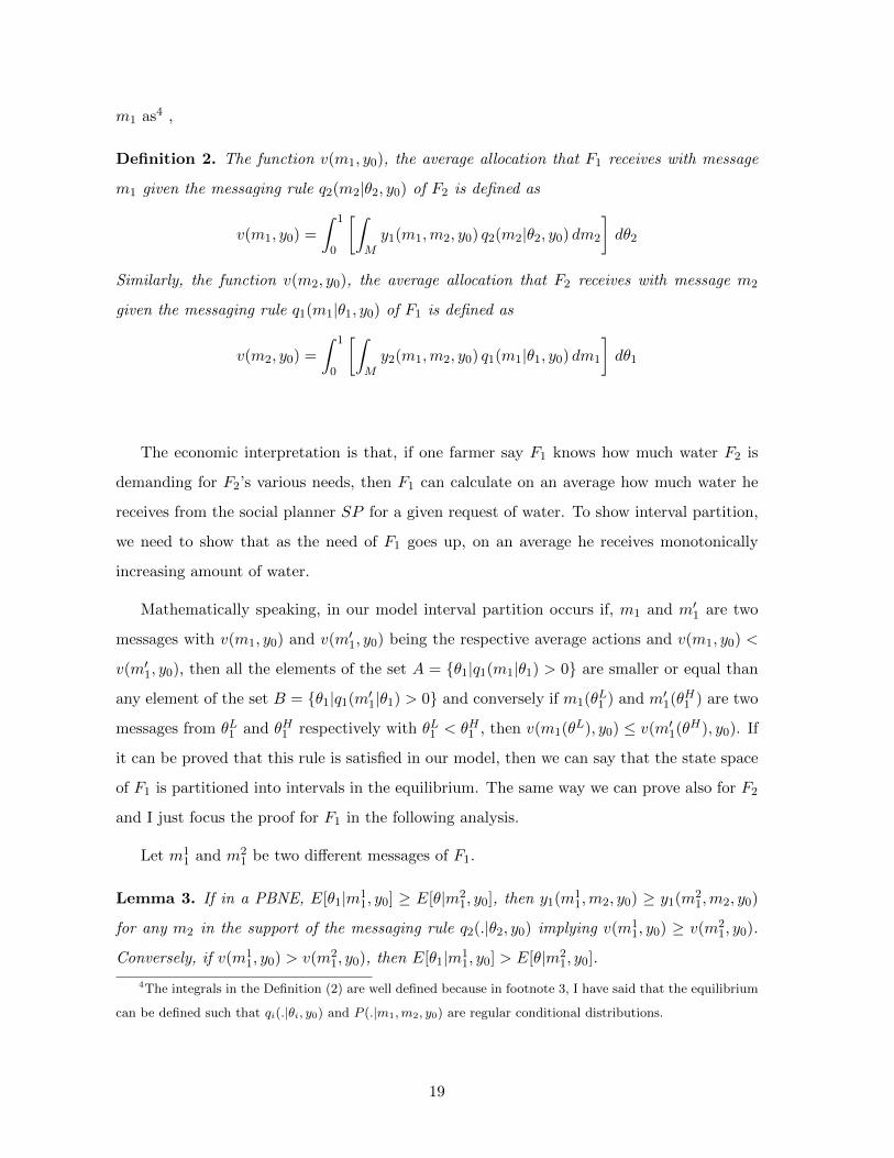
and I just focus the proof for F1 in the following analysis.

Let m11 and m2

1 be two different messages of F1.

Lemma 3. If in a PBNE, E[θ1|m11, y0] ≥ E[θ|m2

1, y0], then y1(m11,m2, y0) ≥ y1(m2

1,m2, y0)

for any m2 in the support of the messaging rule q2(.|θ2, y0) implying v(m11, y0) ≥ v(m2

1, y0).

Conversely, if v(m11, y0) > v(m2

1, y0), then E[θ1|m11, y0] > E[θ|m2

1, y0].

4The integrals in the Definition (2) are well defined because in footnote 3, I have said that the equilibrium

can be defined such that qi(.|θi, y0) and P (.|m1,m2, y0) are regular conditional distributions.

19

The above lemma is quite straightforward because since E[θ1|m1, y0] is the expected value

of the states from which the message m1 has been sent, the message which signals a higher

expected state induces a higher action from SP for a given message of F2 because of the

utility function of SP . In other words, for a given need of F2, if the need of F1 increases,

then he receives more allocation from the social planner. Similarly, if v(m11, y0) > v(m2

1, y0),

then for some m2 ∈ M , we have y1(m11,m2, y0) > y1(m2

1,m2, y0) from definition of v(m, y0)

which can happen only if E[θ1|m11, y0] > E[θ1|m2

1, y0]. This means if F1 receives on an average

a higher allocation, this is due to the fact that his average need gets higher. We shall use

this lemma to prove the following lemma which states that in our model we have interval

partition. The proof is in the appendix and I want to remind again that all the proofs for F1

holds for F2.

Lemma 4. If the messages m1(θL1 ) and m1(θH1 ) are from the states θL1 and θH1 respectively

with θL1 < θH1 , then v(m1(θL1 ), y0) ≤ v(m1(θH1 ), y0). Conversely, if for two messages mL1 and

mH1 , we have v(mL

1 , y0) < v(mH1 , y0), then all the elements of the set A = {θ1|q1(mL

1 |θ1) > 0}

are smaller or equal than any element of the set B = {θ1|q1(mH1 |θ1) > 0}.

The above lemma holds because SP updates his belief using Bayes rule after hearing a

message and the continuity of the utility function of F1 in θ1. Economically speaking, if a

message of F1 has come from a higher need, it induces a higher average allocation to F1 by SP

than a message coming from a lower need. Conversely, if the average allocation is higher for

message mH1 than message mL

1 , then it means that the message mH1 comes when F1 requires

higher amount. We can conclude from this lemma that v(m(θ), y0) which is the average

allocation is monotonically increasing in the need θ where m(θ) comes from the equilibrium

signaling rule.

1.4 Effect of Budget on Information Transmission

Here I show the effect of budget on information transmission with two types of equilibria

given by: (1) Only one of the farmers reveals his state completely (2) Each farmer partitions

the state space into two intervals. The information transmission is measured by the ex-ante

expected utility of a player. This is because the negative of the ex-ante expected utility

calculates the expected value of the square of the distance between the actions from the true

20

states. If the negative of ex-ante expected utility is higher, it means the actions are closer

to the true states (on an average). If the actions are closer to the true states, then it means

that the farmers are giving more information which helps the social planner SP to update

his belief about the true states more accurately and take actions close to the true states.

Hence the information transmission is measured in terms of ex-ante expected utility. The

ex-ante expected utility (EU) of players for our model is given by following Crawford and

Sobel (1982) [7] (CS),

EUF1 =∫θ1∈Θ1

∫m1∈M

[∫θ2∈Θ2

∫m2∈M

(y1(m1,m2, y0)− θ1)2 q2(m2|θ2, y0) dm2 dθ2

]q1(m1|θ1, y0) dm1 dθ1

Similarly, the ex-ante expected utility of F2 (we denote it as EUF2) is defined and the ex-ante

expected utility of SP (we denote it as EUSP ) is the sum of the ex-ante expected utilities of

F1 and F2 i.e. EUSP = EUF1 + EUF2 .

1.4.1 Equilibrium where One Farmer Reveals Fully

We have seen before in the Lemma (2) that both the farmers can not reveal their needs

completely. Consider F2 sending messages with a signaling rule q2(.|θ2, y0) and F1 reveals his

state completely (any bijection from Θ1 →M) and so we can assume θ1 = m1 which we have

discussed before in detail. The social planner SP ’s actions are given by equations (1.2) and

(1.3).

Let a partition of state space θ2 be denoted by b0 = 1, b1, b2, ...., bN = 0 for a given y0.

The following proposition describes the equilibrium where F1 fully reveals his state and the

proof is provided in the appendix. The proof also holds for F2 as we can interchange F1 with

F2 as they are in the same strategic position.

Proposition 3. For 1.5 ≤ y0 < 2, there exists a class of equilibria where F1 tells truth. The

class of equilibria is given by,

1. The strategy of F1 is to send m1 = θ1

2. There exists a positive integer N(y0) such that for every N with 1 ≤ N ≤ N(y0), there

exists a partition b0 = 1, b1, b2, ...., bN = 0 of state space θ2 where the strategy of F2 is

21

to send a message with signaling rule, q2(m2|θ2, y0) such that q2(m2|θ2, y0) is uniform,

supported on [bj , bj+1], if θ2 ∈ (bj , bj+1).

3. N(y0) =⌊

11−(2y0−3)

⌋where bxc is the greatest integer less than or equal to x.

4. The partition satisfies the condition b1+b02 + 1 ≤ y0.

5. Actions of SP are given by y1(θ1, [bj , bj+1], y0) = θ1 and y2(θ1, [bj , bj+1], y0) =bj+bj+1

2

when m2 ∈ [bj , bj+1]. The partition points are given by, bj = N−jN .

The above lemma is quite simple to understand because given F1 sends the true message

θ1, the condition b1+b02 + 1 ≤ y0 ensures that we are always inside the budget. This is

because b1+b02 is the maximum amount F2 receives and the maximum value of θ1 = 1 and

so we should have b1+b02 + 1 ≤ y0. If this condition is not satisfied, then F1 can not reveal

truthfully as he prefers to deviate for high value of θ1. Since we are always within the budget

limit, y2(θ1, [bj , bj+1], y0) =bj+bj+1

2 as F2 asks uniformly between bj and bj+1. The intervals

are equally spaced for F2 which is given by bj = N−jN because we are inside the budget

limit. There is a maximum value of the number of intervals of F2 because F2 can not reveal

completely once F1 reveals completely and within a budget limit we can have only finite

number of equally spaced intervals.

The following corollary describes the effect of y0 on information transmission and the

proof is provided in the appendix.

Corollary 4. Consider the class of equilibria described in Proposition (3). As y0 increases,

N(y0) which is the maximum number of partitions possible, increases. The ex-ante expected

utilities of players are EUF1 = 0, EUF2 = − 112(N(y0))2

, EUSP = − 112(N(y0))2

.

This means a higher y0 allows more information transmission in terms of ex-ante expected

utility to all the players because with a higher y0, the number of equally spaced intervalsN(y0)

of the state space of F2 increases. So with an increase in N(y0), EUF1 stays constant (which

is 0), EUF2 and EUSP increases.

1.4.2 {2} × {2} Symmetric Equilibria

Here I analyze the PBNE where each farmer partitions his state space into two intervals. Let

a2 = 0, a1, a0 = 1 are the interval points for F1 and b0 = 1, b1, b2 = 1 are the interval points

22

for F2 (in our notations a0 and b0 always denotes the right end of the interval which is 1). I

consider the symmetric equilibria and limit my analysis for y0 ≥ 1 to keep the calculations

simple. We need to find the point a1 = b1 which is given in the following proposition and the

proof is given in the appendix.

Proposition 5. For y0 ≥ 1.5, the {2} × {2} symmetric equilibrium is given by a1 = b1 = 12 .

For 1 ≤ y0 ≤ 1.5, a1 = b1 is given by the real solution of the cubic equation 3a31 − a2

1(4y0 +

1) + a1(y20 + 4y0 − 1)− y2

0 = 0.

The ex-ante expected utility for y0 ≥ 1.5 is given by,

EUF1 = EUF2 = −∫ 1

2

0(0.25− θ1)2 dθ1 −

∫ 1

12

(0.75− θ1)2 dθ1 = − 1

48

For the social planner SP , EUSP = EUS1 + EUS2 = − 124 .

Consider Figure (1.2). For 1 ≤ y0 ≤ 1.5, as y0 moves from 1 to 1.5, a1 increases from 0.405

to 0.5 which means the ex-ante expected utility increases. Because as a1 moves closer to the

center 0.5, the ex-ante expected utility of each farmer (which measures the negative of the

expected value of the square of the distance between the actions and the states) gets higher.

I have plotted EUSP in Figure (1.2). For each farmer Fi i = 1, 2, EUFi = 12EU

SP . So in

the {2} × {2} symmetric equilibrium, ex-ante expected utility increases for all players with

increase in y0 from 1 ≤ y0 ≤ 1.5 and then remains constant for 1.5 ≤ y0 ≤ 2. This reaffirms

the conclusion of Corollary (4) that a higher budget increases information transmission for

all players.

1.1 1.2 1.3 1.4 1.5y0

0.42

0.44

0.46

0.48

0.50

a1

1.1 1.2 1.3 1.4 1.5y0

-0.07

-0.06

-0.05

-0.04

-0.03

-0.02

-0.01

EUSP

Figure 1.2: Plot of a1 and EUSP for the {2} × {2} symmetric equilibrium

23

2 by 2 equilibrium

one farmer reveals fully

1.6 1.7 1.8 1.9 2.0y0

-0.08

-0.06

-0.04

-0.02

EUSP

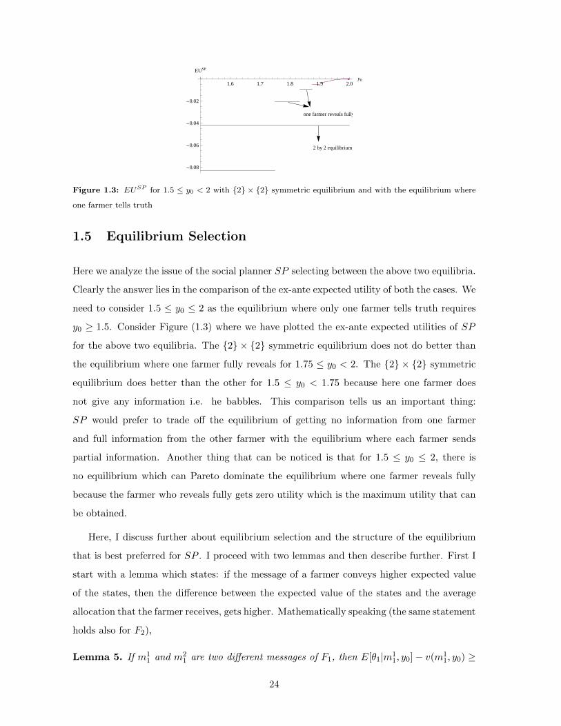
Figure 1.3: EUSP for 1.5 ≤ y0 < 2 with {2} × {2} symmetric equilibrium and with the equilibrium where

one farmer tells truth

1.5 Equilibrium Selection

Here we analyze the issue of the social planner SP selecting between the above two equilibria.

Clearly the answer lies in the comparison of the ex-ante expected utility of both the cases. We

need to consider 1.5 ≤ y0 ≤ 2 as the equilibrium where only one farmer tells truth requires

y0 ≥ 1.5. Consider Figure (1.3) where we have plotted the ex-ante expected utilities of SP

for the above two equilibria. The {2} × {2} symmetric equilibrium does not do better than

the equilibrium where one farmer fully reveals for 1.75 ≤ y0 < 2. The {2} × {2} symmetric

equilibrium does better than the other for 1.5 ≤ y0 < 1.75 because here one farmer does

not give any information i.e. he babbles. This comparison tells us an important thing:

SP would prefer to trade off the equilibrium of getting no information from one farmer

and full information from the other farmer with the equilibrium where each farmer sends

partial information. Another thing that can be noticed is that for 1.5 ≤ y0 ≤ 2, there is

no equilibrium which can Pareto dominate the equilibrium where one farmer reveals fully

because the farmer who reveals fully gets zero utility which is the maximum utility that can

be obtained.

Here, I discuss further about equilibrium selection and the structure of the equilibrium

that is best preferred for SP . I proceed with two lemmas and then describe further. First I

start with a lemma which states: if the message of a farmer conveys higher expected value

of the states, then the difference between the expected value of the states and the average

allocation that the farmer receives, gets higher. Mathematically speaking (the same statement

holds also for F2),

Lemma 5. If m11 and m2

1 are two different messages of F1, then E[θ1|m11, y0]− v(m1

1, y0) ≥

24

E[θ1|m21, y0]− v(m2

1, y0) if E[θ1|m11, y0] > E[θ1|m2

1, y0].

This lemma is straightforward because for a given messagem2 ∈M of F2, if E[θ1|m11, y0] >

E[θ1|m21, y0], then the distance between the θ1 coordinate of the projection of the point

(E[θ1|m11, y0], E[θ2|m2, y0]) on the budget line and E[θ1|m1

1, y0] is higher than the distance

between the θ1 coordinate of the projection of the point (E[θ1|m11, y0], E[θ2|m2, y0]) and

E[θ1|m21, y0]. We can take help of the Figure (1.1) to see it graphically.

Economically speaking, if F2 asks for a fixed amount, then as the need of F1 gets higher,

then the difference between his need and the allocation that he receives increases. This is

because SP has to keep in mind the budget constraint and also the benefit of F2. This

lemma tells us many things, consider the model of Alonso et al. (2008) [2], in their model the

choice of the Head Quarter Manager (for us SP ) and the divisional manager (for us farmer)

coincides for some θ and as θ increases the choices differ more. This leads to partition into

infinite intervals of the state space of the divisional manager. I also expect the same things

to happen in our model that is there is an equilibrium where there is infinite intervals of

the state space of each farmer (but not that both of them tell truth, which can not happen

due to Lemma (2)). Let in our model, F1 tells the true state θ1 in the equilibrium for a

given messaging rule q2(.|θ2, y0) of F2. Let also m11 and m2

1 be two messages from θ11 and

θ21 respectively with θ1

1 > θ21. Since F1 tells the true state, we have E[θ1

1|m11, y0] = θ1

1 and

E[θ21|m2

1, y0] = θ21. Then the above Lemma (5) tells us that θ1

1 − v(m11, y0) ≥ θ2

1 − v(m21, y0)

which means the difference between the need of F1 and the allocation he receives increases

as his need goes up similar to the paper of Alonso et al. (2008) [2]. But then the question

is, does there exist also states like them where if F1 tells the true state, then the average

allocation that F1 receives from SP and the need of F1 coincides given the messaging rule

q2(.|θ2, y0) of F2. The answer is yes and the points are given by 0 ≤ θ1 ≤ θ1 where θ1 is given

by,

θ1 = arg maxθ1

[v(θ1, y0) = θ1]

Here we take m1(θ1) = θ1 as F1 tells truth and so v(m1(θ1), y0) = v(θ1, y0). Since at θ1, the

need of F1 and the allocation he receives coincides, for all 0 ≤ θ1 ≤ θ1, they must coincide

also because we are within the budget limit. The point θ1 exists because at θ1 = 0 which is

the preferred choice of F1, if F1 tells the true state, then SP would like to allocate F1 zero

amount whatever the messaging rule of F2 and so arg max exists. All the above arguments

25

hold if we interchange F1 and F2 as they are strategically equivalent.

In the following lemma, I show that if an equilibrium with infinite intervals exists, then the

length of partition intervals decreases from right side (from 1 on the θ1 axis) and converges to

the point θ1. Since all the equilibrium have interval partition structure, we have two messages

m11 and m2

1 such that v(m11) 6= v(m2

1) from Lemma (4).

Lemma 6. If v(m11, y0) > v(m2

1, y0) and v(m21, y0) < E[θ1|m2

1, y0], then v(m21, y0) < E[θ1|m2

1, y0] <

v(m11, y0) < E[θ1|m1

1, y0]. If there are infinite intervals of the state space Θ1 in the equilibrium,

then for θ1 ≥ θ1, interval points converge to θ1 which implies there will be truth revelation

for θ1 ≤ θ1.

The proof of this lemma is given in the appendix and the same lemma can be stated

for F2 also. The interpretation of this lemma is as follows: v(m11, y0) and v(m2

1, y0) are the

average allocations that F1 receives by sending messages m11 and m2

1 respectively. We can

see that due to budget constraint as well as the quadratic loss utility function, v(m1) can

never exceed E[θ1|m1, y0]. So it holds always that v(m21, y0) ≤ E[θ1|m2

1, y0] and v(m11) ≤

E[θ1|m11, y0]. But once we assume v(m2

1, y0) < E[θ1|m21, y0], then it must be that v(m1

1, y0) <

E[θ1|m11, y0] because once the allocation is strictly less than need, then as the need goes

up allocation can not be equal to need due to rationality. Assume to the contradiction

that, E[θ1|m21, y0] ≥ v(m1

1, y0). This means that the message m21 is sent from some states

θ1 ≥ v(m11, y0). Then for those states θ1 ≥ v(m1

1, y0), it is better to send m11 than m2

1 so

that the allocation is closer to their need. Suppose there exists an equilibrium with infinite

partitions, then it can never converge towards the right side (towards 1) on the state space

[0, 1] and will always converge to the left side 0. This is because convergence requires that the

distance between successive E[θ1|m1(θ1), y0] decreases in the direction of convergence. But

from Lemma (5), the monotonicity (increasing) of E[θ1|m1(θ1), y0] with increase in θ1 and

the fact E[θ1|m21, y0] < v(m1

1, y0) < E[θ1|m11, y0], it can never converge towards right side. So

it has to converge towards the left side, i.e. towards 0. But it has to also converge at θ1,

otherwise the indifference condition demands that for θ1 ≤ θ1, the intervals will be equally

spaced because we are within the budget limit and hence there can not be infinite intervals.

Since F1 and F2 are strategically equivalent, the same arguments can be used for F2 as we

have always said throughout our paper.

So the above discussions point out that there may exist an equilibrium with infinite

26

intervals of the state spaces of both the farmers. Let ai, i ∈ N be the interval points of

F1 and bj , j ∈ N be the interval points of F2. The computation of the interval points ai

of F1 and bj of F2 from the indifference or no-incentive conditions are particularly difficult.

Because first the indifference conditions are cubic equations in the interval points as evident

from the {2} × {2} symmetric equilibrium. Solving a system of cubic equations with many

unknowns is analytically tough. Second how to choose in which regions of the state space the

point y1([ai, ai+1], [bj , bj+1], y0) belongs i.e. whether y1([ai, ai+1], [bj , bj+1], y0) = ai+ai+1

2 or

ai+ai−1

2 −ai+ai−1

2+

bj+bj+12

−y02 or 0 or y0 as there are so many possibilities, but all may not give

feasible solutions. So it is analytically challenging to compute the ex-ante expected utilities

of different equilibria with different number of interval points and compare them to select the

best equilibrium.

Following Proposition 2 of Alonso et al. (2008) [2], I conjecture that there exists a

symmetric equilibria with infinite intervals of the state spaces of both the farmers which

gives highest ex-ante expected utility to the social planner SP . Let a symmetric grid of state

space Θ = Θ1 × Θ2 be given by a partition of state space Θ1 by a0 = 1, a1, a2, ..., ai, ...

and a partition of state space Θ2 be denoted by a0 = 1, a1, a2, ..., ai, .... The graphical

illustration of a symmetric equilibrium with infinite intervals is provided in the Figure (1.4).

We can calculate that the point to which the intervals converge is given by, θ1 = θ2 =

min{max{0, y0 − 1+a12 }, 1} from the definition which can be easily seen in the figure also.

1.6 Conclusion

I discussed a model of distribution of a limited resource among multiple senders by a receiver

in the context of water allocation to farmers (senders) by the social planner (receiver). I

illustrated that with a budget constraint, there is no fully revealing PBNE. I further proved

the interval partition structure of all equilibria. I showed that higher budget facilitates

information transmission with an equilibrium where only one farmer reveals truthfully and

with a {2}×{2} symmetric equilibrium. I compared the ex-ante expected utility of the social

planner for these two equilibria and showed that she prefers the equilibrium where both the

farmers send partial information than the equilibrium where one farmer tells the true state

and the other farmer babbles. Then I provided arguments that there may be equilibria with

27

θ2

θ1

C = (1, 0)

A = (0, 1)

y0

F

B = (1, 1)

a1

(a1+1)2

a1 (a1+1)2

O

P

a2a3a4y0 − (a1+1)2

y0 − (a1+1)2

a2

a3

a4

Figure 1.4: Infinite intervals of both the state spaces

infinite intervals of both the state spaces of the farmers.

The computation of equilibria in our model is analytically challenging as I have described

before. I conjecture that the equilibrium which gives highest ex-ante expected utility to the

social planner is a symmetric equilibrium with infinite intervals. I have provided arguments

that point to the existence of infinite equilibria in our model, but I have not yet provided a

formal proof of it. The future research can focus on providing a formal proof on the existence

of equilibria with infinite intervals of both the state spaces using the lattice theory approach

adopted in Gordon (2010)[13]. Also we can verify the claim of the conjecture whether a

symmetric equilibrium with infinite intervals is the best choice for the social planner. We

may use some numerical techniques to consider for different number of symmetric intervals,

calculate the ex-ante expected utilities. In this way, if we are able to show that as the number

of intervals increases, the ex-ante expected utility of the receiver increases, then it will provide

28

more evidence in favor of the conjecture. Another claim which can be looked at is that for one

farmer, the best equilibrium is where he has infinite intervals and the other farmer babbles.

More research can also focus on the case where the social planner is not utilitarian (does

not give equal weights to each farmer), she gives different weights to the utilities of the

farmers. In this way, we may perform some comparative statics like the effect of weight

on fully revelation and equilibrium selection. Also some standard research like the role of

sequential communication, where only one farmer is informed about the other farmer’s state,

where both the farmers know about their states can be investigated.

1.7 Appendix

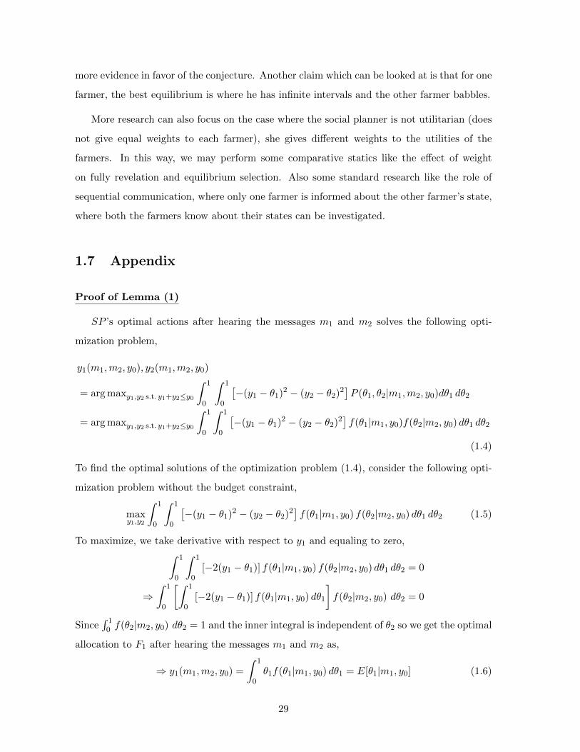
Proof of Lemma (1)

SP ’s optimal actions after hearing the messages m1 and m2 solves the following opti-

mization problem,

y1(m1,m2, y0), y2(m1,m2, y0)

= arg maxy1,y2 s.t. y1+y2≤y0

∫ 1

0

∫ 1

0

[−(y1 − θ1)2 − (y2 − θ2)2

]P (θ1, θ2|m1,m2, y0)dθ1 dθ2

= arg maxy1,y2 s.t. y1+y2≤y0

∫ 1

0

∫ 1

0

[−(y1 − θ1)2 − (y2 − θ2)2

]f(θ1|m1, y0)f(θ2|m2, y0) dθ1 dθ2

(1.4)

To find the optimal solutions of the optimization problem (1.4), consider the following opti-

mization problem without the budget constraint,

maxy1,y2

∫ 1

0

∫ 1

0

[−(y1 − θ1)2 − (y2 − θ2)2

]f(θ1|m1, y0) f(θ2|m2, y0) dθ1 dθ2 (1.5)

To maximize, we take derivative with respect to y1 and equaling to zero,∫ 1

0

∫ 1

0[−2(y1 − θ1)] f(θ1|m1, y0) f(θ2|m2, y0) dθ1 dθ2 = 0

⇒∫ 1

0

[∫ 1

0[−2(y1 − θ1)] f(θ1|m1, y0) dθ1

]f(θ2|m2, y0) dθ2 = 0

Since∫ 1

0 f(θ2|m2, y0) dθ2 = 1 and the inner integral is independent of θ2 so we get the optimal

allocation to F1 after hearing the messages m1 and m2 as,

⇒ y1(m1,m2, y0) =

∫ 1

0θ1f(θ1|m1, y0) dθ1 = E[θ1|m1, y0] (1.6)

29

Similarly taking derivate with respect to y2 and equaling to zero we get,

y2(m1,m2, y0) =

∫ 1

0θ2f(θ2|m2, y0) dθ2 = E[θ2|m2, y0] (1.7)

If the above optimal solutions satisfy y1 +y2 ≤ y0 then it is the solution to the social planner’s

optimization problem, otherwise we consider the following optimization problem.

max0≤y1≤y0

∫ 1

0

∫ 1

0

[−(y1 − θ1)2 − (y0 − y1 − θ2)2

]f(θ1|m1, y0) f(θ2|m2, y0) dθ1 dθ2 (1.8)

Taking derivative with respect to y1 and equaling to zero,∫ 1

0

∫ 1

0[−2(y1 − θ1) + 2(y0 − y1 − θ2)] f(θ1|m1, y0) f(θ2|m2, y0) dθ1 dθ2 = 0

⇒ y1 =y0

2+

∫ 1

0

∫ 1

0(θ1 − θ2)f(θ1|m1, y0) f(θ2|m2, y0) dθ1 dθ2

=y0

2+E[θ1|m1, y0]

2− E[θ2|m2, y0]

2

But as 0 ≤ y1 ≤ y0, the optimal solutions are,

y1(m1,m2, y0) = min

[max

(0,y0

2+E[θ1|m1, y0]

2− E[θ2|m2, y0]

2

), y0

](1.9)

y2(m1,m2, y0) = y0 − y1(m1,m2, y0) = min

[max

(0,y0

2+E[θ2|m2, y0]

2− E[θ1|m1, y0]

2

), y0

](1.10)

To find equation (1.10), use different cases of equation (1.9). If we write in compact form of

both the cases of optimal solutions y1 + y2 ≤ y0 and y1 + y2 ≥ y0, the solution is given by

similar to equation (1.1),

y1(m1,m2, y0) = min

[max

(0, E[θ1|m1, y0]−max

(0,E[θ1|m1, y0] + E[θ2|m2, y0]− y0

2

)), y0

]y2(m1,m2, y0) = min

[max

(0, E[θ2|m2, y0]−max

(0,E[θ1|m1, y0] + E[θ2|m2, y0]− y0

2

)), y0

]

Proof of Lemma (2)

30

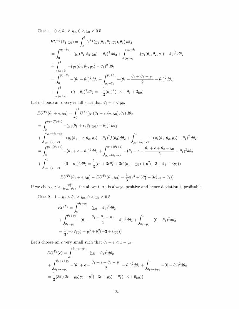
Case 1 : 0 < θ1 < y0, 0 < y0 < 0.5

EUF1(θ1, y0) =

∫ 1

0UF1(y1(θ1, θ2, y0), θ1) dθ2

=

∫ y0−θ1

0−(y1(θ1, θ2, y0)− θ1)2 dθ2 +

∫ y0+θ1

y0−θ1−(y1(θ1, θ2, y0)− θ1)2 dθ2

+

∫ 1

y0+θ1

−(y1(θ1, θ2, y0)− θ1)2 dθ2

=

∫ y0−θ1

0−(θ1 − θ1)2dθ2 +

∫ y0+θ1

y0−θ1−(θ1 −

θ1 + θ2 − y0

2− θ1)2dθ2

+

∫ 1

y0+θ1

−(0− θ1)2dθ2 = −1

3(θ1)2(−3 + θ1 + 3y0)

Let’s choose an ε very small such that θ1 + ε < y0.

EUF1(θ1 + ε, y0) =

∫ 1

0UF1(y1(θ1 + ε, θ2, y0), θ1) dθ2

=

∫ y0−(θ1+ε)

0−(y1(θ1 + ε, θ2, y0)− θ1)2 dθ2

+

∫ y0+(θ1+ε)

y0−(θ1+ε)−(y1(θ1 + ε, θ2, y0)− θ1)2f(θ2)dθ2 +

∫ 1

y0+(θ1+ε)−(y1(θ1, θ2, y0)− θ1)2 dθ2

=

∫ y0−(θ1+ε)

0−(θ1 + ε− θ1)2dθ2 +

∫ y0+(θ1+ε)

y0−(θ1+ε)−(θ1 + ε− θ1 + ε+ θ2 − y0

2− θ1)2dθ2

+

∫ 1

y0+(θ1+ε)−(0− θ1)2dθ2 =

1

3(ε3 + 3εθ2

1 + 3ε2(θ1 − y0) + θ21(−3 + θ1 + 3y0))

EUF1(θ1 + ε, y0)− EUF1(θ1, y0) =1

3ε(ε2 + 3θ2

1 − 3ε(y0 − θ1))

If we choose ε <3θ21

3(y0−θ1) , the above term is always positive and hence deviation is profitable.

Case 2 : 1− y0 > θ1 ≥ y0, 0 < y0 < 0.5

EUF1 =

∫ θ1−y0

0−(y0 − θ1)2dθ2

+

∫ θ1+y0

θ1−y0−(θ1 −

θ1 + θ2 − y0

2− θ1)2dθ2 +

∫ 1

θ1+y0

−(0− θ1)2dθ2

=1

3(−3θ1y

20 + y3

0 + θ21(−3 + 6y0))

Let’s choose an ε very small such that θ1 + ε < 1− y0.

EUF1(ε) =

∫ θ1+ε−y0

0−(y0 − θ1)2dθ2

+

∫ θ1+ε+y0

θ1+ε−y0−(θ1 + ε− θ1 + ε+ θ2 − y0

2− θ1)2dθ2 +

∫ 1

θ1+ε+y0

−(0− θ1)2dθ2

=1

3(3θ1(2ε− y0)y0 + y2

0(−3ε+ y0) + θ21(−3 + 6y0))

31

EUF1(ε)− EUF1 = ε(2θ1 − y0)y0

The above term is always positive and hence deviation is profitable.

Case 3 : 1− y0 ≤ θ1 < 1, y0 ≤ 0.5

EUF1 =

∫ θ1−y0

0−(y0 − θ1)2dθ2

+

∫ 1

θ1−y0−(θ1 −

θ1 + θ2 − y0

2− θ1)2dθ2 =

1

12(−4(θ1 − y0)3 − (1 + θ1 − y0)3)

Let’s choose an ε very small such that θ1 + ε < 1.

EUF1(ε) =

∫ θ1+ε−y0

0−(y0 − θ1)2dθ2

+

∫ 1

θ1+ε−y0−(θ1 + ε− θ1 + ε+ θ2 − y0

2− θ1)2dθ2

= −(θ1 − y0)2(ε+ θ1 − y0) +1

12(8(θ1 − y0)3 + (−1 + ε− θ1 + y0)3)

EUF1(ε)− EUF1 =1

12ε(3 + 6(θ1 − y0)− 9(θ1 − y0)2 + ε2 − 3ε(1 + θ1 − y0))

The above term is positive as if we take ε < 3+6(θ1−y0)−9(θ1−y0)2

3(1+θ1−y0) and so a deviation is prof-

itable.

Case 4 : 0 < θ1 < 1− y0, 0.5 < y0 < 1

EUF1(θ1, y0) =

∫ y0−θ1

0−(θ1 − θ1)2dθ2

+

∫ y0+θ1

y0−θ1−(θ1 −

θ1 + θ2 − y0

2− θ1)2dθ2 +

∫ 1

y0+θ1

−(0− θ1)2dθ2

= −1

3(θ1)2(−3 + θ1 + 3y0)

Let’s choose an ε very small such that θ1 + ε < y0.

EUF1(θ1 + ε, y0) =

∫ y0−(θ1+ε)

0−(θ1 + ε− θ1)2dθ2

+

∫ y0+(θ1+ε)

y0−(θ1+ε)−(θ1 + ε− θ1 + ε+ θ2 − y0

2− θ1)2dθ2 +

∫ 1

y0+(θ1+ε)−(0− θ1)2dθ2

=2ε3

3+

2θ31

3+ ε2(−θ1 + y0)− θ2

1(−1 + ε+ θ1 + y0)

EUF1(θ1 + ε, y0)− EUF1(θ1, y0) = −2ε3

3+ εθ2

1 + ε2(θ1 − y0)

32

Case 5 : y0 > θ1 ≥ 1− y0, 0.5 < y0 < 1

EUF1 =

∫ y0−θ1

0−(θ1 − θ1)2dθ2

+

∫ 1

y0−θ1−(θ1 −

θ1 + θ2 − y0

2− θ1)2dθ2 =

1

12(8(θ1 − y0)3 − (1 + θ1 − y0)3)

Let’s choose an ε very small such that θ1 + ε < y0.

EUF1(ε) =

∫ y0−θ1−ε

0−(θ1 + ε− θ1)2dθ2

+

∫ 1

y0−θ1−ε−(θ1 + ε− θ1 + ε+ θ2 − y0

2− θ1)2dθ2

= ε2(ε+ θ1 − y0) +1

12(−8ε3 + (−1 + ε− θ1 + y0)3)

EUF1(ε)− EUF1 =1

12ε(5ε2 + ε(−3− 9(y0 − θ1)) + 3(1 + θ1 − y0)2)

The above term is positive for ε < 3(1+θ1−y0)2

3+9(y0−θ1) and hence deviation is profitable.

Case 6 : y0 ≤ θ1 < 1, 0.5 ≤ y0 < 1

EUF1 =

∫ θ1−y0

0−(y0 − θ1)2dθ2

+

∫ 1

θ1−y0−(θ1 −

θ1 + θ2 − y0

2− θ1)2dθ2 =

1

12(−4(θ1 − y0)3 − (1 + θ1 − y0)3)

Let’s choose an ε very small such that θ1 + ε < 1.

EUF1(ε) =

∫ θ1+ε−y0

0−(y0 − θ1)2dθ2

+

∫ 1

θ1+ε−y0−(θ1 + ε− θ1 + ε+ θ2 − y0

2− θ1)2dθ2

= −(θ1 − y0)2(ε+ θ1 − y0) +1

12(8(θ1 − y0)3 + (−1 + ε− θ1 + y0)3)

EUF1(ε)− EUF1 =1

12ε(3 + 6(θ1 − y0)− 9(θ1 − y0)2 + ε2 − 3ε(1 + θ1 − y0))

The above term is positive as if we take ε < 3+6(θ1−y0)−9(θ1−y0)2

3(1+θ1−y0) and so a deviation is prof-

itable.

Case 7 : y0 − 1 ≥ θ1 > 0, 2 > y0 > 1

EUF1 =

∫ 1

0−(θ1 − θ1)2dθ2 = 0

This is the maximum utility that can be obtained and hence deviation is not profitable.

33

Case 8 : y0 − 1 < θ1 < 1, 2 > y0 ≥ 1

EUF1 =

∫ y0−θ1

0−(θ1 − θ1)2dθ2

=

∫ 1

y0−θ1−(θ1 −

θ1 + θ2 − y0

2− θ1)2dθ2 = − 1

12(1 + θ1 − y0)3

Let’s choose an ε very small such that θ1 + ε < 1.

EUF1(ε) =

∫ y0−θ1−ε

0−(θ1 + ε− θ1)2dθ2

+

∫ 1

y0−θ1−ε−(θ1 + ε− θ1 + ε+ θ2 − y0

2− θ1)2dθ2

= ε2(ε+ θ1 − y0) +1

12(−8ε3 + (−1 + ε− θ1 + y0)3)

EUF1(ε)− EUF1 =1

12ε(5ε2 + ε(−3− 9(y0 − θ1)) + 3(1 + θ1 − y0)2)

The above term is positive for ε < 3(1+θ1−y0)2

3+9(y0−θ1) and hence deviation is profitable.

So we have analyzed all cases and proved the stated lemma.

Proof of Lemma (3)

It can be easily proved using the formula for optimal action given in equation (1.2) for

all possible cases. If E[θ1|m11, y0] = E[θ1|m2

1, y0], then y1(m11,m2, y0) = y1(m2

1,m2, y0). If

E[θ1|m11, y0] > E[θ1|m2

1, y0] and E[θ1|m11, y0] + E[θ2|m2, y0] − y0 ≤ 0, then E[θ1|m2

1, y0] +

E[θ2|m2, y0] − y0 ≤ 0 and so we have y1(m11,m2, y0) = E[θ1|m1

1, y0] > y1(m21,m2, y0) =

E[θ1|m21, y0]. Similarly we can consider other cases and prove it. But the result can be

seen conveniently graphically because y1(m1,m2, y0) is the orthogonal projection of the point

(E[θ1|m1, y0], E[θ1|m2, y0]) on to the budget line. For the converse, if v(m11, y0) > v(m2

1, y0),

then for some m2 ∈ M2, we have y1(m11,m2, y0) > y1(m2

1,m2, y0) from the definition of

v(m, y0). If we refer the equation (1.2) for y1(m1,m2, y0), we can immediately derive that

E[θ1|m11, y0] > E[θ1|m2

1, y0].

Proof of Lemma (4)

If E[θ1|m1(θL1 ), y0) ≤ E[θ1|m1(θH1 ), y0], then from Lemma (3), v(m1(θL1 ), y0) ≤ v(m1(θH1 ), y0).

So we assume E[θ1|m1(θL1 ), y0] > E[θ1|m1(θH1 ), y0]. Let’s prove by contradiction and assume

that v(m1(θL1 ), y0) > v(m1(θH1 ), y0) which implies for some m2 ∈ M , y1(m1(θL1 ),m2, y0) >

34

y1(m1(θH1 ),m2, y0). Since F1 prefers m1(θH1 ) at θH1 we have,,

−∫ 1

0

[∫M

(y1(m1(θH1 ),m2, y0)− θH1 )2q2(m2|θ2, y0) dm2

]dθ2

> −∫ 1

0

[∫M

(y1(m1(θL1 ),m2, y0)− θH1 )2q2(m2|θ2, y0) dm2

]dθ2

⇒ θH1 <

∫ 10

[∫M

((y1(m1(θH1 ),m2, y0))2 − (y1(m1(θL1 ),m2, y0))2

)q2(m2|θ2, y0) dm2

]dθ2

2∫ 1

0

[∫M

(y1(m1(θH1 ),m2, y0)− y1(m1(θL1 ),m2, y0)

)q2(m2|θ2, y0) dm2

]dθ2

We have taken the strict relation because for somem2 ∈M2, y1(m1(θL1 ),m2, y0) > y1(m1(θH1 ),m2, y0).

Since F1 prefers m1(θL1 ) at θL1 we also have,

−∫ 1

0

[∫M

(y1(m1(θL1 ),m2, y0)− θL1 )2q2(m2|θ2, y0) dm2

]dθ2

> −∫ 1

0

[∫M

(y1(m1(θH1 ),m2, y0)− θL1 )2q2(m2|θ2, y0) dm2

]dθ2

⇒ θL1 >

∫ 10

[∫M

((y1(m1(θH1 ),m2, y0))2 − (y1(m1(θL1 ),m2, y0))2

)q2(m2|θ2, y0) dm2

]dθ2

2∫ 1

0

[∫M

(y1(m1(θH1 ),m2, y0)− y1(m1(θL1 ),m2, y0)

)q2(m2|θ2, y0) dm2

]dθ2

The above relations imply θL1 > θH1 which is a contradiction.

Conversely, let v(mL1 , y0) < v(mH

1 , y0), then for somem2 ∈M2, y1(mL1 ,m2, y0) < y1(mH

1 ,m2, y0).

Let θL1 be any state from which mL1 is sent and θH1 be any state from which mH

1 is sent. Then

we can calculate like the above relations (just the signs reversed) to conclude that θL1 < θH1

which completes the proof.

Proof of Proposition (3)

Notice that for y0 ≥ 2, both the farmers will tell truth as I have said before. So we

focus on 1.5 ≤ y0 < 2 and the condition why the limit 1.5 has been set will be clear later.

Given the farmers’ strategies, the best actions of the social planner are y1(θ1,m2, y0) = θ1

and y2(θ1,m2, y0) =bj+bj+1

2 if m2 ∈ [bj , bj+1] from equations (1.2) and (1.3). The condi-

tion b1+b02 + 1 ≤ y0 makes sure that the optimal actions satisfy the budget constraint as

y1(θ1,m2, y0) = θ1 ≤ 1 and the maximum value of y2(θ1,m2, y0) = b1+b02 when m2 ∈ [b1, b0].

If we do not impose the condition b1+b02 + 1 ≤ y0, then the optimal solutions for 1 > θ1 ≥

y0 − b1+b02 are given by y1 = θ1+y0

2 − bj+1+bj4 and y2 = y0−θ1

2 +bj+1+bj

4 from equations (1.2)

and (1.3). But these actions by SP can not be part of equilibrium as F1 will find it profitable

to inflate the message to get closer to his optimal action y1 = θ1 as here SP ’s optimal action

y1 = θ1+y02 − bj+1+bj

4 = θ1 −θ1+

bj+1+bj2

2 < θ1.

35

Now to make F2 incentive compatible at the partition points, his utility at bj , between

sending a message in [bj−1, bj ] and [bj , bj+1] should be same and following Crawford and Sobel

(1982)[7], the indifference condition for F2 is given for j = 0, 1, .., N − 1 by,

UF2(y2(θ1, [bj , bj+1], y0), bj+1) = US2(y2(θ1, [bj+1, bj+2], y0), bj+1)

⇒ −(bj + bj+1

2− bj+1)2 = −(

bj+1 + bj+2

2− bj+1)2

⇒ bj + bj+1

2− bj + 1 =

bj+1 + bj+2

2− bj+1

⇒ bj+1 =bj + bj+2

2

Since b0 = 1 then from bj+1 =bj+bj+2

2 we get, b1 = 1+b22 , ...., bj = 1 − j + b1j and bN =

1 − N + b1N . As bN = 0, we get, b1 = N−1N . Substituting backwards, we have, bj =

1− j + N−1N j = N−j

N . Consider the condition b1+b02 + 1 ≤ y0. Putting the value of b1 and b0,

we get,N−1N

+1

2 + 1 ≤ y0 which gives, N ≤ 11−(2y0−3) . So the N(y0) stated in the proposition

is N(y0) =⌊

11−(2y0−3)

⌋where bxc denotes the greatest integer lower or equal to x. For each

1 ≤ N ≤ N(y0), we can describe a partition and the partition points can be calculated as

done above. Notice that as y0 < 1.5, then N(y0) = 0, but it is impossible as the minimum

value of N is 1 which means there is no partition. So we have considered y0 ≥ 1.5. The other

way of looking at it is if F1 tells truth and if F2 does not send any information (he blabbers),

then the best action for SP is to take y2 = 0.5 which will require at least y0 = 1.5 when

θ1 = 1.

Proof of Corollary (4)

I have established during the proof of the proposition that N(y0) =⌊

11−(2y0−3)

⌋. As y0

increases, it is clear that N(y0) increases. For y0 = 1.5, N(y0) = 1. If we set N(y0) = 2,

we get y0 = 1.75 and at y0 ≈ 1.833, N(y0) = 3. As y0 → 2, we get that N(y0) → ∞ which

satisfies the observation that there will be fully revelation when y0 = 2. Since F1 reveals

truthfully, EUF1 = 0.

EUF2 = −∑N(y0)

j=0

∫ N(y0)−jN(y0)

N(y0)−(j+1)N(y0)

(2N(y0)−(2j+1)2N(y0) − θ1)2 dθ1

=∑N(y0)

j=0

[(2N(y0)−(2j+1)

2N(y0)−θ1)3

3

]N(y0)−jN(y0)

N(y0)−(j+1)N(y0)

= 13

∑N(y0)j=0 ( −1

2N(y0))3 − ( 12N(y0))3

= 13

−2(N(y0))3

N(y0) = − 112(N(y0))2

Proof of Proposition (5)

36

With {2}×{2} symmetric equilibrium, the intervals are [a2 = 0, a1], [a1, a0 = 1] for F1 and

the mid points are a12 and 1+a1

2 respectively. Similarly for F2, the intervals are [b2 = 0, b1],

[b1, b0 = 1] and the mid points are b12 and 1+b1

2 respectively. So the points to calculate

the actions of SP that we consider are, (a12 ,b12 ), (a12 ,

1+b12 ), (1+a1

2 , b12 ) and (1+a12 , 1+b1

2 ). Let

(θ1, θ2) be any point. The optimal action of SP in the direction of θ1 which is y1 can be

any of 0, y0, θ1 − θ1+θ12 or θ1 and similarly the optimal action of SP in the direction of

θ2 which is y2 can be any of 0, y0, θ2 − θ1+θ22 or θ2. The actions taken by SP for our

above four points can be any of these values, but all may not give meaningful solutions. I

considered all the possibilities and the only feasible solution (y1, y2) for 1.5 ≤ y0 ≤ 2 is given

by the actions same as the points which means from the indifference condition of F1 that

a1 = b1 = 12 . For 1 ≤ y0 ≤ 1.5, the feasible solution is given by the actions as follows: for

(a12 ,b12 ) is same ((a12 ,

b12 )), for (a12 ,

1+b12 ) is same (a12 ,

1+b12 ), for (1+a1

2 , b12 ) is same (1+a12 , b12 )

and for (1+a12 , 1+b1

2 ) is (a1+12 −

a1+12

+b1+1

2−y0

2 , b1+12 −

a1+12

+b1+1

2−y0

2 ) and so the indifference

condition for F1 is given by (for F2, we have the same equation when we consider symmetric

equilibrium where a1 = b1),

−(a1 + 1

2− a1)2b1 − (

a1 + 1

2−

a1+12 + b1+1

2 − y0

2− a1)2(1− b1) = −(

a1

2− a1)2

Setting a1 = b1, we get

3a31 − a2

1(4y0 + 1) + a1(y20 + 4y0 − 1)− y2

0 = 0

For 1 ≤ y0 ≤ 1.5, we have a value of a1 which satisfies the above equation.

Proof of Lemma (5)

Consider two messagesm11 andm2

1 in the equilibrium such that E[θ1|m11, y0] > E[θ1|m2

1, y0].

Now we have,

E[θ1|m11, y0]− v(m1

1, y0) ≥ E[θ1|m21, y0]− v(m2

1, y0)

⇒ E[θ1|m11, y0]−

∫ 10

[∫M2

y1(m11,m2, y0)q2(m2|θ2, y0) dm2

]dθ2

≥ E[θ1|m21, y0]−

∫ 10

[∫M2

y1(m21,m2, y0)q2(m2|θ2, y0) dm2

]dθ2

⇒∫ 1

0

[∫M (E[θ1|m1

1, y0]− y1(m11,m2, y0))q2(m2|θ2, y0) dm2

]dθ2

≥∫ 1

0

[∫M (E[θ1|m2

1, y0]− y1(m21,m2, y0))q2(m2|θ2, y0) dm2

]dθ2

37

Now we can substitute the value of y1(m1,m2, y0) from equation (1.2) into the above equation

and see that the above equation always holds when E[θ1|m11, y0] > E[θ1|m2

1, y0].

Proof of Lemma (6)

If v(m11, y0) > v(m2

1, y0) and v(m21, y0) < E[θ1|m2

1, y0], then for somem2 ∈M , y1(m21,m2, y0) <

E[θ1|m21, y0] which implies for the same m2 ∈ M , we have y1(m1

1,m2, y0) < E[θ1|m11, y0] as

E[θ1|m11, y0] ≥ E[θ1|m2

1, y0] from equation (1.2). So we have v(m11, y0) < E[θ1|m1

1, y0] and we

just need to show E[θ1|m21, y0] < v(m1

1, y0). It can be seen from above (during the proof of

Lemma (4) in the appendix) that m21 is sent below

θ1 =

∫ 10

[∫M

((y1(m1

1,m2, y0))2 − (y1(m21,m2, y0))2

)q2(m2|θ2, y0) dm2

]dθ2

2∫ 1

0

[∫M

(y1(m1

1,m2, y0)− y1(m21,m2, y0)

)q2(m2|θ2, y0) dm2

]dθ2

The message m21 is sent for states above and below θ1 = E[θ1|m2

1] and so we have,

E[θ1|m21] <

∫ 10

[∫M

((y1(m1

1,m2, y0))2 − (y1(m21,m2, y0))2

)q2(m2|θ2, y0) dm2

]dθ2

2∫ 1

0

[∫M

(y1(m1

1,m2, y0)− y1(m21,m2, y0)

)q2(m2|θ2, y0) dm2

]dθ2

Now I aim to show that∫ 10

[∫M

((y1(m1

1,m2, y0))2 − (y1(m21,m2, y0))2

)q2(m2|θ2, y0) dm2

]dθ2

2∫ 1

0

[∫M

(y1(m1

1,m2, y0)− y1(m21,m2, y0)

)q2(m2|θ2, y0) dm2

]dθ2

< v(m11)

. i.e.∫ 10

[∫M

((y1(m1

1,m2, y0))2 − (y1(m21,m2, y0))2

)q2(m2|θ2, y0) dm2

]dθ2∫ 1

0

[∫M

(y1(m1

1,m2, y0)− y1(m21,m2, y0)

)q2(m2|θ2, y0) dm2

]dθ2

< 2

∫ 1

0

[∫My1(m1

1,m2, y0)q2(m2|θ2, y0) dm2

]dθ2

⇒∫ 1

0

∫M

(y1(m1

1,m2, y0)− y1(m21,m2, y0)

)(y1(m1

1,m2, y0) + y1(m21,m2, y0)

)q2(m2|θ2, y0) dm2 dθ2

< (

∫ 1

0

∫M

(y1(m1

1,m2, y0)− y1(m21,m2, y0)

)q2(m2|θ2, y0) dm2 dθ2)

(2

∫ 1

0

∫My1(m1

1,m2, y0)q2(m2|θ2, y0) dm2 dθ2)

⇒∫ 1

0

∫M

(y1(m1

1,m2, y0)− y1(m21,m2, y0)

)(y1(m1

1,m2, y0) + y1(m21,m2, y0)

)q2(m2|θ2, y0) dm2 dθ2

< (

∫ 1

0

∫M

(y1(m1

1,m2, y0)− y1(m21,m2, y0)

)q2(m2|θ2, y0) dm2 dθ2)

(

∫ 1

0

∫M

(y1(m11,m2, y0) + y1(m1

1,m2, y0))q2(m2|θ2, y0) dm2 dθ2)

38

The above holds by triangle inequality for integration and the fact that y1(m11,m2, y0) ≥

y1(m21,m2, y0) for each m2 ∈ M and so we have E[θ1|m2

1, y0] < v(m11, y0). Now I want to

show if there exists infinite intervals of the state space Θ1, then for θ1 ≥ θ1 whether interval

points converge to θ1 which implies there will be truth revelation for θ1 ≤ θ1. If interval

points converge to a point, from Lemma (5) and the fact that E[θ1|m21, y0] < v(m1

1, y0) <

E[θ1|m11, y0], we can see that interval points can converge only to the left side direction

(towards 0 on the θ1 axis) and not to the right side direction. Assume the interval points do

not converge to θ1, then we can see from the indifference condition of S1 that there will be

only finite intervals and so we can not have truth revelation for θ1 ≤ θ1.

39

Chapter 2

Cheap Talk with Correlated Signals

Abstarct: In this chapter1, we consider an information aggregation setting where the signals

of the senders and receivers are correlated. The correlation arises due to the fact that some

players may collect information from the same source. For one sender and one receiver case,

we show that the threshold of the bias for truth telling monotonically decreases as correlation

increases. We generalize the model to arbitrary number of senders and one receiver with a

single correlation parameter to keep the analysis tractable. We show that the threshold of the

bias for truth telling is non monotonic for senders more than three due to overshooting effect.

Considering the fact that low bias comes with high correlation (because people with similar

preferences access same sources of information), we characterize the choice of senders/discus-

sion partners in terms of level of correlation and polarization in the society and highlight the

effect of non-monotonicity of threshold in the selection of a group of senders.

JEL Code : C72, D82, D83

Keywords : Cheap Talk, Multiple Senders, Correlation

2.1 Introduction

In organizations, discussion groups or committees, there are situations where a partially

informed receiver (who receives information) aggregates information from partially informed

1A joint work with Sergio Currarini, Ca’ Foscari University of Venice and Giovanni Ursino, Catholic

University of Milan

41

senders (who sends information) before taking a decision. However, it may be that the

information of the receiver and the information of the sender is correlated. In this paper,

we investigate the role of correlation on strategic communication (Cheap Talk) and how it

affects the appointment of a group of senders/discussion partners/experts.

The natural questions that one can ask, why correlation in the information arises and

what is its role on communication. Correlation in the information arises because the sender

(he) and the receiver (she) may be accessing the same source for collecting information. The

example of this is: if both the receiver and the sender are leftists, they may be accessing left-

leaning newspapers to access information. Also if the receiver and the sender have common

acquaintances, then their information is correlated. The role of correlation on communica-

tion is that it decreases the informativeness of the messages that the sender sends to the

receiver. So when the receiver collects an information from the sender, she has to discount

the correlated part of the information before taking the decision. Since the messages of the

sender is not that informative, it causes a welfare loss to both the receiver and the sender.

To introduce correlation into the theoretical framework, we adopt the binary signals

framework that is discussed in the paper by Morgan and Stocken (2008) [20] in the context

of information aggregation. In their paper, the signals of the sender and the receiver are

conditionally independent. To incorporate correlation into their binary signals framework,

we consider the paper by Bahadur (1961) [5] that first discusses correlation among binary

signals. A single correlation parameter naturally occurs for two players where the correlation

parameter denotes the probability that both the players collect signals from the same source

and with complementary probability they collect from independent sources. We consider

only positive correlation. When the number of players increase, we need many correlation

parameters to describe the probabilities with which different partitions of the set of players

occur. The partitions are used to describe correlation because members in the same group

in a partition collect information from the same source and the information of each group is

independent of the information of any other group. Since the number of partitions increases

as the number of players increase, this makes the model non tractable. To have a tractable

model with a single correlation parameter for more than two players and to keep all the

players equivalent in the information structure, we assume that either all the players collect

information from the same source or all of them collect from independent sources. The

42

correlation parameter denotes the probability with which one of these two events occurs.

The structure and the main results of the paper are as follows:

• We start with a model of one receiver and a sender where both of them receive partial

correlated information. We show that as correlation increases, the threshold of the bias

for truth telling decreases monotonically due to overshooting effect. This is because as

the information gets more correlated, sending a false message does not elicit a much

different action than the true message.

• Then we consider the receiver’s problem of selecting the sender. Since correlation de-

creases the informative content of the messages, it causes an welfare less. In the absence

of any external constraint, the receiver would choose a sender with zero correlation and

the bias within the truth telling threshold. We consider an external constraint where

people with close preferences (bias) have large correlation. This happens due to the

fact that they access same source of information (people with leftist ideology access

left-leaning newspapers). This imposes a restriction that the receiver while choosing a

sender with low correlation has to take into account that the bias also becomes large

and the bias may lie outside the truth telling threshold.

• We show that a generalized increase of correlation (for each given bias, correlation

increases by same amount) has effect on bias or homophily (measures the similarity in

the preferences of people). If the equilibrium is a corner solution, then a generalized

increase of correlation decreases the homophily (the bias increases). If the equilibrium is

an interior solution, then a generalized increase of correlation increases the homophily.

• We further show that a change in the level of polarization (measures the ratio of corre-

lation of people with high biases and the correlation of people with low biases) has an

effect on homophily. If the solution is a corner solution, then a change in the level of

polarization (keeping the level of correlation fixed) has no effect on homophily. If the

solution is an interior solution, then an increase in the level of polarization decreases

the homophily.

• Then we generalized the model of two players to arbitrary number of players. We show

that for more than three players, increase in correlation has non monotonic effect on the

43

threshold of bias for truth telling due to overshooting effect. As correlation increases

from zero, the threshold decreases and after certain point of correlation (which we call

as critical value) it reverses and the threshold increases. There is a particular value of

correlation where the threshold is unbounded.

• We consider the receiver’s problem of choosing a discussion group where the discussion

groups vary in their correlation. All the members in the discussion group have same

preference and each group has same number of members. We consider the external

constraint like the two players case where low bias comes with high correlation in the

information.

• We show that the same analysis like the two players case holds for a generalized increase

of correlation as long as the correlation of the optimal solution is smaller than the critical

value where the threshold is minimum. When the correlation of the optimal solution is

greater than the critical value, then a generalized increase of correlation (keeping the

level of polarization fixed) decreases the homophily.

• We again show that the same analysis like the two players case also holds for an increase

in the level of polarization as long as the correlation of the optimal solution is smaller

than the critical value where the threshold is minimum. When the correlation of the

optimal solution is greater than the critical value, then an increase in the level of

polarization (keeping the level of correlation fixed) increases the homophily.

Since our paper incorporates correlation in the information, it is a more general discussion

of the works by Morgan and Stocken (2008) [20] and Galeotti et al. (2011) [10]. All the issues

that they consider in their papers can be studied in our framework when there is correlation

in the information structure.

2.2 Model with Two Players

There are two agents, a Sender S (he) and a Receiver R (she). R takes an action y ∈ R

which has a direct impact on both players’ utilities. These also depend on the true state of

the world, θ which is unknown to both players and such that θ ∼ U [0, 1]. Before R takes

44

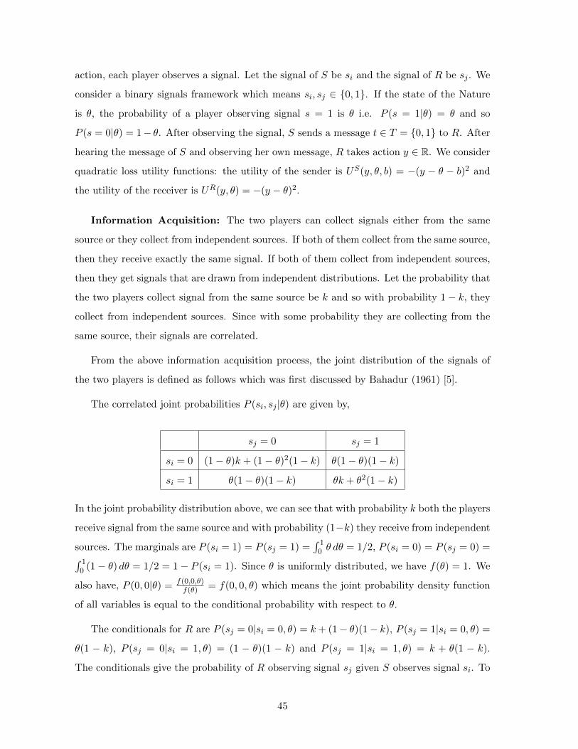
action, each player observes a signal. Let the signal of S be si and the signal of R be sj . We

consider a binary signals framework which means si, sj ∈ {0, 1}. If the state of the Nature

is θ, the probability of a player observing signal s = 1 is θ i.e. P (s = 1|θ) = θ and so

P (s = 0|θ) = 1− θ. After observing the signal, S sends a message t ∈ T = {0, 1} to R. After

hearing the message of S and observing her own message, R takes action y ∈ R. We consider

quadratic loss utility functions: the utility of the sender is US(y, θ, b) = −(y − θ − b)2 and

the utility of the receiver is UR(y, θ) = −(y − θ)2.

Information Acquisition: The two players can collect signals either from the same

source or they collect from independent sources. If both of them collect from the same source,

then they receive exactly the same signal. If both of them collect from independent sources,

then they get signals that are drawn from independent distributions. Let the probability that

the two players collect signal from the same source be k and so with probability 1− k, they

collect from independent sources. Since with some probability they are collecting from the

same source, their signals are correlated.

From the above information acquisition process, the joint distribution of the signals of

the two players is defined as follows which was first discussed by Bahadur (1961) [5].

The correlated joint probabilities P (si, sj |θ) are given by,

sj = 0 sj = 1

si = 0 (1− θ)k + (1− θ)2(1− k) θ(1− θ)(1− k)

si = 1 θ(1− θ)(1− k) θk + θ2(1− k)

In the joint probability distribution above, we can see that with probability k both the players

receive signal from the same source and with probability (1−k) they receive from independent

sources. The marginals are P (si = 1) = P (sj = 1) =∫ 1

0 θ dθ = 1/2, P (si = 0) = P (sj = 0) =∫ 10 (1− θ) dθ = 1/2 = 1− P (si = 1). Since θ is uniformly distributed, we have f(θ) = 1. We

also have, P (0, 0|θ) = f(0,0,θ)f(θ) = f(0, 0, θ) which means the joint probability density function

of all variables is equal to the conditional probability with respect to θ.

The conditionals for R are P (sj = 0|si = 0, θ) = k+ (1− θ)(1− k), P (sj = 1|si = 0, θ) =

θ(1 − k), P (sj = 0|si = 1, θ) = (1 − θ)(1 − k) and P (sj = 1|si = 1, θ) = k + θ(1 − k).

The conditionals give the probability of R observing signal sj given S observes signal si. To

45

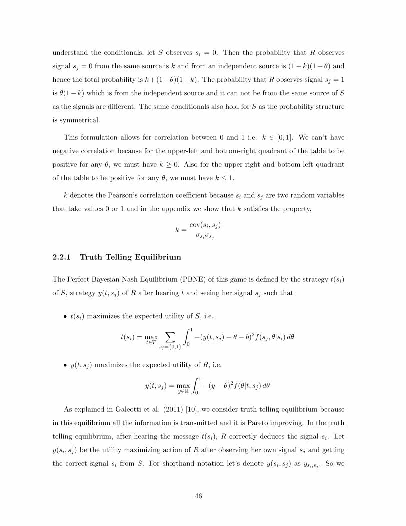
understand the conditionals, let S observes si = 0. Then the probability that R observes

signal sj = 0 from the same source is k and from an independent source is (1− k)(1− θ) and

hence the total probability is k+(1−θ)(1−k). The probability that R observes signal sj = 1

is θ(1− k) which is from the independent source and it can not be from the same source of S

as the signals are different. The same conditionals also hold for S as the probability structure

is symmetrical.

This formulation allows for correlation between 0 and 1 i.e. k ∈ [0, 1]. We can’t have

negative correlation because for the upper-left and bottom-right quadrant of the table to be

positive for any θ, we must have k ≥ 0. Also for the upper-right and bottom-left quadrant

of the table to be positive for any θ, we must have k ≤ 1.

k denotes the Pearson’s correlation coefficient because si and sj are two random variables

that take values 0 or 1 and in the appendix we show that k satisfies the property,

k =cov(si, sj)

σsiσsj

2.2.1 Truth Telling Equilibrium

The Perfect Bayesian Nash Equilibrium (PBNE) of this game is defined by the strategy t(si)

of S, strategy y(t, sj) of R after hearing t and seeing her signal sj such that

• t(si) maximizes the expected utility of S, i.e.

t(si) = maxt∈T

∑sj={0,1}

∫ 1

0−(y(t, sj)− θ − b)2f(sj , θ|si) dθ

• y(t, sj) maximizes the expected utility of R, i.e.

y(t, sj) = maxy∈R

∫ 1

0−(y − θ)2f(θ|t, sj) dθ

As explained in Galeotti et al. (2011) [10], we consider truth telling equilibrium because

in this equilibrium all the information is transmitted and it is Pareto improving. In the truth

telling equilibrium, after hearing the message t(si), R correctly deduces the signal si. Let

y(si, sj) be the utility maximizing action of R after observing her own signal sj and getting

the correct signal si from S. For shorthand notation let’s denote y(si, sj) as ysi,sj . So we

46

have,

ysi,sj = maxy∈R

∫ 1

0−(y − θ)2f(θ|si, sj) dθ

⇒ ysi,sj = E[θ|si, sj ] =

∫ 1

0θf(θ|si, sj) dθ (2.1)

We also know that

f(θ|si, sj) =P (si, sj |θ)∫ 10 P (si, sj |θ)

To derive ysi,sj , we need to calculate f(θ|si, sj), for different values of si and sj and then

using it we derive ysi,sj . In the appendix we have derived the values of ysi,sj and they are:

y0,0 =1 + k

2(2 + k), y0,1 =

1

2, y1,0 =

1

2, y1,1 =

3 + k

2(2 + k)

We can see that the actions (y0,0 and y1,1) when all signals are same is a function of k, this

is because when the receiver R receives all the signals same in the truth telling equilibrium,

she believes that with probability k they have acquired the information from the same source

and with 1 − k, they have acquired from independent sources. The actions (y0,1 and y1,0)

when the signals are different is independent of k, because R believes that they have acquired

the information from independent sources with full probability. Also we can check that

y0,0 < y0,1 < y1,1 for all k ∈ [0, 1]; this is an important observation which will be used later

while explaining the overshooting effect.

Threshold of Bias

S reports signal si truthfully (i.e. there is a bijection from the messages to the true signals)

and not 1− si if, the following indifference or no-incentive condition holds,

∑sj∈{0,1}

∫ 1

0−(ysi,sj − θ − b)2f(sj , θ|si) dθ ≥

∑sj∈{0,1}

∫ 1

0−(y1−si,sj − θ − b)2f(sj , θ|si) dθ

47

⇒∑

sj∈{0,1}

∫ 1

0−(ysi,sj − θ − b)2f(θ|si, sj)P (sj |si) dθ ≥

∑sj∈{0,1}

∫ 1

0−(y1−si,sj − θ − b)2f(θ|si, sj)P (sj |si) dθ

⇒∑

sj∈{0,1}

−(ysi,sj − E[θ|si, sj ]− b)2 P (sj |si) ≥∑

sj∈{0,1}

−(y1−si,sj − E[θ|si, sj ]− b)2 P (sj |si)

Since ysi,sj = E[θ|si, sj ], substituting this in the above no-incentive condition, we have,

∑sj∈{0,1}

(y1−si,sj − ysi,sj )2

2P (sj |si) ≥ b

∑sj∈{0,1}

(y1−si,sj − ysi,sj )P (sj |si) (2.2)

To compute P (sj |si), we know that f(si, sj , θ) = f(si, sj |θ) and P (si) = 12 and so we

have,

P (sj |si) =

∫ 1

0f(sj , θ|si) dθ =

∫ 1

0

f(si, sj , θ)

P (si)dθ =

∫ 1

0

P (si, sj |θ)1/2

dθ = 2

∫ 1

0P (si, sj |θ) dθ

We substitute the values of ysi,sj and P (sj |si) in the no-incentive condition (2.2) to find

the threshold of b for truth telling2. Given si = 0, we get the threshold for truth telling as,

b ≤ 1

8 + 4k(2.3)

Given si = 1, from the indifference condition, we have for truth telling,

b ≥ − 1

8 + 4k(2.4)

From equations (2.3) and (2.4), the threshold band of b for truth telling is given by,

‖b‖ ≤∥∥∥∥ 1

8 + 4k

∥∥∥∥ (2.5)

The above discussion can be summarized in the following proposition:

Proposition 6. As the correlation in the information between the sender and the receiver

increases, the threshold band of the bias decreases for truth-telling.

2For k = 1, both the players receive same signals. So when R observes her own signal, she exactly knows

the signal of S and hence does not take into account the message of S while taking the action. So for k = 1

we do not consider truth-telling equilibrium conditions.

48

The intuition of the equations (2.3) and (2.4) which is summarized in the above proposi-

tion will be explained below while discussing the overshooting effect.

It can be observed immediately that when k = 0, we have ‖b‖ ≤∥∥1

8

∥∥ which is the same

result as in Morgan and Stocken (2008) [20] and Galeotti et al. (2011) [10] where they have

considered independent signals meaning zero correlation. So our framework is a more general

framework of the binary signals framework to analyze cheap talk.

Overshooting Effect

The overshooting effect for the sender can be defined as: when the sender sends a false

message instead of the true message, then the utility does not increase.

We know from before,

y0,0 =1 + k

2(2 + k), y0,1 =

1

2, y1,0 =

1

2, y1,1 =

3 + k

2(2 + k)

Here, y1,0 − y0,0 = 12(2+k) > 0 and y1,1 − y1,0 = 1

2(2+k) > 0 for all k ∈ [0, 1] and as k

increases both the terms decreases.

Consider si = 0 and b > 0. It can be seen from the values of ysi,sj that the actions induced

with the true message are smaller than the false message and for a given k, the difference

is same for any sj . The threshold for overshooting effect (where sending the false message

does not improve the utility and hence deviation is not profitable) decreases when k increases

because actions induced by the false message gets closer to the actions induced by the true

message. This explains the equation (2.3). We can explain the negative threshold of b < 0

given in equation (2.4) by using si = 1 and doing similar analysis. Both these equations have

been combined to form Proposition (6).

In the following section, we use our above framework of correlation to address some issues

regarding the choice of senders/discussion partners as a way to acquire information.

2.2.2 Selecting Correlation

In this section, we discuss the problem of the the receiver selecting a sender for information

aggregation. If the senders’ biases are within the threshold level, then how much correlation

49

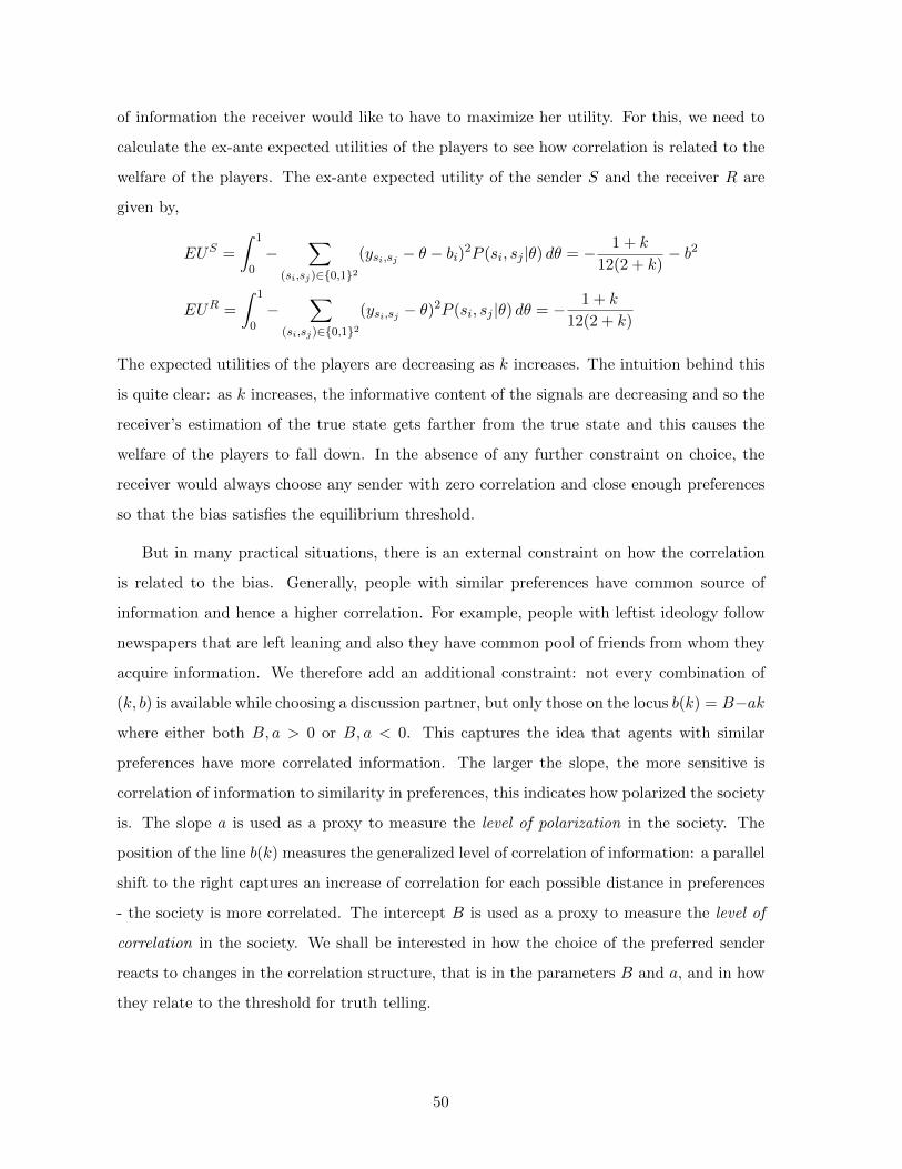
of information the receiver would like to have to maximize her utility. For this, we need to

calculate the ex-ante expected utilities of the players to see how correlation is related to the

welfare of the players. The ex-ante expected utility of the sender S and the receiver R are

given by,

EUS =

∫ 1

0−

∑(si,sj)∈{0,1}2

(ysi,sj − θ − bi)2P (si, sj |θ) dθ = − 1 + k

12(2 + k)− b2

EUR =

∫ 1

0−

∑(si,sj)∈{0,1}2

(ysi,sj − θ)2P (si, sj |θ) dθ = − 1 + k

12(2 + k)

The expected utilities of the players are decreasing as k increases. The intuition behind this

is quite clear: as k increases, the informative content of the signals are decreasing and so the

receiver’s estimation of the true state gets farther from the true state and this causes the

welfare of the players to fall down. In the absence of any further constraint on choice, the

receiver would always choose any sender with zero correlation and close enough preferences

so that the bias satisfies the equilibrium threshold.

But in many practical situations, there is an external constraint on how the correlation

is related to the bias. Generally, people with similar preferences have common source of

information and hence a higher correlation. For example, people with leftist ideology follow

newspapers that are left leaning and also they have common pool of friends from whom they

acquire information. We therefore add an additional constraint: not every combination of

(k, b) is available while choosing a discussion partner, but only those on the locus b(k) = B−ak

where either both B, a > 0 or B, a < 0. This captures the idea that agents with similar

preferences have more correlated information. The larger the slope, the more sensitive is

correlation of information to similarity in preferences, this indicates how polarized the society

is. The slope a is used as a proxy to measure the level of polarization in the society. The

position of the line b(k) measures the generalized level of correlation of information: a parallel

shift to the right captures an increase of correlation for each possible distance in preferences

- the society is more correlated. The intercept B is used as a proxy to measure the level of

correlation in the society. We shall be interested in how the choice of the preferred sender

reacts to changes in the correlation structure, that is in the parameters B and a, and in how

they relate to the threshold for truth telling.

50

Change in the Level of Correlation

B6

B5

B4

b = 18

slope = −a

Threshold of bfor truth telling

B3

B2

B1O1 O2 O3

shift

kSelecting Correlation for two players case

b

Parallel

Figure 2.1: The effect of change in B fixing a with B, a > 0

Let’s assume that B, a > 0 and we consider an increase in the level of correlation (B)

fixing the level of polarization (a) i.e. a generalized increase of correlation (parallel rightward

shift of the line b(k) = B − ak). The effect of the rightward shift in b(k) on homophily (how

close the preferences are) is opposite depending on which equilibrium we are at (whether at

the corner solutions or interior solutions). We explain the effect of rightward shift with the

help of Figure (2.1). Let’s consider the line B1−ak where B1 is less than b = 18 (the threshold

at k = 0) and in this case the receiver can select the sender with zero correlation and the

equilibrium point is (0, B1) which is a corner solution. As B1 increases to B2 and then to

B3, the equilibrium point move to (0, B2) and then to (0, B3). So an increase in B where B

is below the threshold level is followed by a decrease in homophily (because the bias of the

equilibrium point increases).

Now let’s consider the line B4 − ak where B4 is greater than b = 18 , then the new

equilibrium point lies at O1 which is an interior solution. As B4 increases to B5 and then

to B6, the equilibrium points move from O1 to O2 and then to O3. We can see that the

correlation of the equilibrium points increases and the bias decreases. So an increase in

51

B where B is above the threshold level is followed by an increase in homophily (the bias

decreases). We can take B, a < 0 (here the level of correlation is −B and polarization is −a)

and doing the same analysis like above, the same implications hold for an increase in −B

keeping a fixed (here we have to consider the threshold in the negative axis).

The conclusions of the above analysis is stated in the following proposition (increase

means a reasonably small increase):

Proposition 7. If the level of correlation is low in the society (corner solution), a generalized

increase of correlation decreases the homophily. If the level of correlation is high in the society

(interior solution), a generalized increase of correlation increases the homophily.

Change in the Level of Polarization

Here we study the effect of change in the level of polarization (a) in the society. Let’s assume

that B, a > 0 and consider a rotation of the line b(k) = B − ak where a increases.

b

B

B1

B1 − a3k

Selection of Correlation for two players casek

B1 − a2k

B − a1k

O1

O for truth tellingThreshold of b

B − ak

Figure 2.2: The effect of rotation of b(k) = B − ak with B, a > 0

Consider the rotation of the line b(k) = B − ak where B is the center of rotation. We

explain the effect of rotation with the help of Figure (2.2). Let the rotated line be B − a1k

where a1 is greater than a. The equilibrium point moves from O to O1 and so correlation

decreases and homophily decreases (the bias increases). Now consider the rotation of the

52

line b(k) = B1 − a2k where B1 lies below the threshold level. The equilibrium point is at B1

which is a corner solution. Then a small change in the level of polarization fixing the point

B1 does not change the equilibrium point B1.

We can take B, a < 0 ( here −B is the level of correlation and −a is the level of polariza-

tion) and the same implications hold while considering an increase in the level of polarization

(for this we have to consider the threshold in the negative axis). The conclusions of the above

analysis is stated in the following proposition (we consider a small increase):

Proposition 8. An increase in the level of polarization decreases the homophily in the society

if the level of correlation is high and when it is low, an increase in the level of polarization

does not have any effect on homophily.

Change in Both the Levels of Correlation and Polarization

Now I analyze rotation around any point on the line b(k) = B − ak which changes both the

level of correlation (B) and the level of polarization (a).

k

for truth telling

B − akL2

b

B

B1

L3

O

B1 − a2k

Threshold of b

L1

O2

O1

Figure 2.3: The effect of rotation of b(k) = B − ak at any point with B, a > 0

Consider Figure (2.3) and the line B − ak intersecting the threshold at point O which is

the optimal solution. If we make a clockwise rotation around the point L1 lying below the

threshold level, then we can see that the optimal point shifts to O1. This means there is an

53

increase in the correlation and an increase in the homophily (the bias decreases).

The reason comes from the fact that the rotation around L1 can be thought of a rotation

around O and then a parallel shift to the right. Here the rotation around O increases the

polarization without changing the bias and the correlation. Then to have the optimal point

at O1, we have to take a parallel shift to the right, this causes the homophily to increase and

correlation to increase (the effect of parallel shift or increase in the level of correlation (B)

has been explained before in Figure (2.1)). The analysis is very similar to the income and

substitution effect in the consumer choice theory. Here for us income effect is the change in

the level of correlation (B) which is the parallel shift and the substitution effect is the change

in the level of polarization (a) which is the rotation around O.

Similarly we can argue that for the rotation around L2, the combined effect of rotation

and parallel shift is a decrease in correlation and a decrease in homophily. This is shown in

the Figure (2.3) where O moves to O2.

2.3 Model with n-Players

Now we generalize the above model to n players. There are n players and all of them receive

a signal either 0 or 1 which depend on the true state of the world, θ which is unknown to

both players and θ ∼ U [0, 1]. We denote the receiver as R and the senders as Si where

i ∈ {1, ..., n − 1}. The signals of the players are given by the n-tuple s = (sR, s1, ...., sn−1)

where sR is the signal of R and the rest are the signals of the senders Si, i ∈ {1, ..., n − 1}.

If the state of the Nature is θ, the probability of a player observing signal s = 1 is θ i.e.

P (s = 1|θ) = θ and so P (s = 0|θ) = 1 − θ. After observing the signal, Si sends a message

ti ∈ T = {0, 1} to R. Let t = (t1, t2, ..., tn−1) be the set of messages that the receiver receives

from the senders. After receiving the messages, R takes an action y ∈ R. The quadratic loss

utility functions are given by, USi(y, θ, bi) = −(y − θ − bi)2 and UR(y, θ) = −(y − θ)2. Let

P (s|θ) denotes the joint probability of the signals of the players given the state θ.

Information Acquisition: The set of n players can be partitioned into different groups

and we have different ways to partition the set. The total number of partitions is given by

the Bell number B(n). A group in a partition can be used to show which players collect

information from the same source. The players who lie in the same group collect information

54

from the same source (get same signal) and the groups collect from independent sources.

When we have only two players, the number of partitions is two which means either both

players receive from the same source or from independent sources; so we need only one

correlation parameter to denote the probability of each partition occurring. As there are large

number of players, the number of partitions are very large which can be see by computing

the Bell number. Therefore we need many correlation parameters where each correlation

parameter is the probability of each partition occurring. So many parameters have the

obvious disadvantage that it leaves the model non tractable. To keep the model tractable, we

consider a simplified structure of information collection where either all players collect from

the same source or they collect from independent sources3. In other words, we allow that

only two partitions of the set of n players can occur (the whole set or the finest set) and the

other partitions never occur.

From the above discussion, the joint probability distribution of the signals with one cor-

relation parameter is given as:P (1, ..., 1|θ) = θn(1− k) + θk

P (0, ..., 0|θ) = (1− θ)n(1− k) + (1− θ)k

P (l(1s), (n− l)(0s)|θ) = θl(1− θ)n−l(1− k) (l 6= 0, n)

(2.6)

(Note: P (l(1s), (n− l)(0s)|θ) is the probability of an ordered sequence containing l ones and

n− l zeros.) The interpretation of the above probabilities is that with probability k, all the

signals come from the same source and with probability 1 − k, all the signals come from

independent sources.

The conditional is given by,

P (l1(1s), l0(0s)|m1(1s),m0(0s), θ)

=P (l1 +m1(1s), l0 +m0(0s), θ)

P (m1(1s),m0(0s), θ)

If m1 6= 0 and m0 6= 0, then P (l1(1s), l0(0s)|m1(1s),m0(0s), θ) = θl1(1− θ)l0 .

If m0 = 0,m1 6= 0, then P (l1(1s), l0(0s)|m1(1s),m0(0s), θ) = P (l1+m1,l0|θ)P (m1|θ)

3We can still have only one correlation parameter where either all players collect from the same source or

some players collect information from the same source and the rest from independent sources. But in this way,

the players do not remain anymore strategically equivalent which in turn makes the analysis complicated.

55

If m0 6= 0,m1 = 0, then P (l1(1s), l0(0s)|m1(1s),m0(0s), θ) = P (l0+m0,l1|θ)P (m0|θ)

The parameter k denotes the Pearson’s correlation coefficient of the joint probability dis-

tribution of any two signals. This is because if we consider the above probability distribution

for n players, the same probability structure also holds for the restricted probability distri-

bution to n − l players which we describe in the following lemma. The proof is provided in

the appendix section.

Lemma 7. P ((n− l) 1s|θ) = θ(n−l)(1− k) + θk

P ((n− l) 0s|θ) = (1− θ)(n−l)(1− k) + (1− θ)k

P ((j) 1s, (n− l − j) 0s|θ) = θj(1− θ)n−l−j(1− k)

(2.7)

So the joint probability distribution P (si, sj |θ) of any two signals si and sj has same

probability distribution like two players case and we have proved before that k denotes the

Pearson’s correlation coefficient.

2.3.1 Truth Telling Equilibrium

The Perfect Bayesian Nash Equilibrium (PBNE) for this game is defined in the same way as

for the two players case except that the senders and the receiver now take into account the

messages of other senders while maximizing their utility functions.

Let t−q be the collection of all messages from senders except tq from sender Sq i.e. t−q =

t\ tq. So t = (tq, t−q). The PBNE of this game is defined by the strategy ti(si) of Si, strategy

y(t, sR) of R after hearing the messages t and seeing her own signal sR such that

• ti(si) maximizes the expected utility of Si, i.e.

ti(si) = maxti∈T

∑(t−i,si)∈{0,1}n−1

∫ 1

0−(y(t, sR)− θ − b)2f(t−i, sR, θ|si) dθ

• y(t, sR) maximizes the expected utility of R, i.e.

y(t, sR) = maxy∈R

∫ 1

0−(y − θ)2f(θ|t, sR) dθ

56

Like the two players case, we consider truth telling equilibrium i.e. after hearing the

message ti(si), R correctly deduces the signal si. Let y(s−R, sR) = y(s) be the utility max-

imizing action of R after observing her own signal sR and getting correct signals s−R from

other senders. For convenience, let’s denote y(s) as ys. So we have,

ys = maxy∈R

∫ 1

0−(y − θ)2f(θ|s) dθ

⇒ ys = E[θ|s] =

∫ 1

0θf(θ|s) dθ

where f(θ|s) = f(s|θ)∫ 10 f(s|θ) dθ

So we can compute ys for various values of s and they are given by,

y1,1,...,1 =2(n+ 1)(3− k + kn)

3(n+ 2)(2− k + kn), y0,0,...,0 =

6 + k(n− 1)(n+ 4)

3(n+ 2)(2− k + kn), yl(1s),(n−l)(0s) =

1 + l

n+ 2

This shows that when the receiver R receives all signals same in the truth telling equilib-

rium, she believes the signals coming from two possibilities, either all of them have gone to

the same source or all of them have accessed independent sources; so the optimal action is

a function of k. But when R receives signals that are not all same, she believes the signals

coming from only independent sources and hence the optimal action does not depend on k.

We can check that when n is fixed and k increases, y0,0,...,0 increases and y1,1,...,1 decreases.

This is because the signals get more correlated and hence when one player receives a signal,

it is more likely that others also get the same signal. When k is fixed and n increases, then

y0,0,...,0 decreases and y1,1,...,1 increases. This is because more players getting the same signal

means either the signal is coming from lower states (for all signals 0) or the signal is coming

from higher states (for signals 1). So k and n have opposite effects on the actions that R

takes and this will have important consequence on the overshooting effect that decides the

threshold of b for truth telling as we shall see in the analysis that follows.

57

Threshold of Bias

Si reports signal si truthfully and not 1− si if, the following no-incentive condition holds4,∫ 1

0−

∑s−i∈{0,1}n−1

(ysi,s−i− θ − bi)2f(s−i, θ|si) dθ

≥∫ 1

0−

∑s−i∈{0,1}n−1

(y1−si,s−i− θ − bi)2f(s−i, θ|si) dθ

We can proceed in the same way like equation (2.2) for the two players case and the above

indifference condition becomes,

∑s−i∈{0,1}n−1

P (s−i|si)42(s−i|si)

2≥ bi

∑s−i∈{0,1}n−1

4(s−i|si)P (s−i|si) (2.8)

where 4(s−i|si) = y1−si,s−i− ysi,s−i

.

Now we derive the threshold of bi for truth telling from the above equation (2.8) which

is given in the following theorem and the proof is given in the appendix. We assume that if

Si is indifferent between sending the messages 0 or 1, then he sends the true message.

Theorem 9. Let 4(s−i|si) = y1−si,s−i− ysi,s−i

. If n and k are such that

∑s−i∈{0,1}n−1

4(s−i|si)P (s−i|si) = 0,

then Si is indifferent between telling si and 1− si for any bias which means bi ∈ (−∞,+∞)

for truth telling. If n and k are such that

∑s−i∈{0,1}n−1

4(s−i|si)P (s−i|si) 6= 0,

then the limit of bi for truth telling is given by,

‖bi‖ ≤ ‖∑

s−i∈{0,1}n−1 P (s−i|si)42(s−i|si)

2∑s−i∈{0,1}n−14(s−i|si)P (s−i|si)

‖

If one remembers clearly the overshooting effect for two players case and how ys changes

when n and k change, then the above theorem should not be looking difficult. However we

4See footnote2

58

explain the intuitions for this theorem in detail afterwards when we discuss the overshooting

effect. Now we calculate explicitly the value of the threshold of bi which is a function of n

and k and the calculations are provided in the appendix.

Let

T (n, k) =

∑s−i∈{0,1}n−1 P (s−i|0)4

2(s−i|0)2∑

s−i∈{0,1}n−14(s−i|0)P (s−i|0)

In the appendix, we show that

T (n, k) =

− 36n+ k(−2 + n)(−1 + n)(12 + k(−17 + k(−5 + n)(−1 + n)(1 + n) + n(−9 + 2n)))

6(2 + k(−1 + n))(2 + n)(−6n+ k(−2 + n)(−1 + n)(−1 + k + kn))

(2.9)

We further show in the appendix that when Si observes si = 0, if T (n, k) ≥ 0, the

threshold for truth telling is given by, bi ≤ T (n, k) and if T (n, k) ≤ 0, then bi ≥ T (n, k).

When Si observes si = 1, if T (n, k) ≥ 0, the threshold for truth telling is given by,

bi ≥ −T (n, k) and if T (n, k) ≤ 0, then bi ≤ −T (n, k).

Combining all the above conditions for truth telling, we get the threshold band of bi for

a given n and k as,

‖bi‖ ≤ ‖T (n, k)‖ (2.10)

All the intuitions for the above results are provided below when we discuss overshooting

effect. We have plotted in Figure (2.4) the threshold band for n = 3, n = 4, n = 5 and

n = 10. In the sub figure where n = 3, the threshold is monotonically decreasing like the two

players case. For n ≥ 4, the threshold is non-monotonic.

Now we find the relation between n and k such that∑

s−i∈{0,1}n−1 4(s−i|si)P (s−i|si) = 0.

From Theorem (9), in this case any bi is allowed for truth telling which means bi is unbounded.

We state in the following proposition for which combinations of n and k, bi is unbounded.

We denote the k for given n where bi is unbounded as k(n).

Proposition 10. For n = 1, 2, 3, bi is bounded always for k ∈ [0, 1]. For n ≥ 4, bi is

unbounded iff

k(n) =(n− 1)(n− 2) +

√(n− 1)2(n− 2)2 + 4.6n.(n− 2)(n− 1)(1 + n)

2(n− 2)(n− 1)(1 + n)(2.11)

59

Threshold for truth telling for n = 3

k

120

b

− 120

b

124

− 124

The threshold for truth telling for n = 4

k1

b

128

− 128

Threshold for truth telling for n = 5

k0.735

b

148

− 148

k

Threshold for truth telling for n = 10

0.325

Figure 2.4: The threshold band for n = 3, n = 4, n = 5 and n = 10

We can verify that in the above proposition (10), k(n) ∈ [0, 1] for n ≥ 4 and as n increases,

k(n) decreases. As n→∞, we can see that k(n)→ 0 for any bi to be allowed for truth telling.

This tells us that if the receiver wants to form a committee of senders containing n−1 number

of senders for any n ≥ 4 where the senders can have any bias, then she can always choose a

k ∈ [0, 1] where n and k satisfy the relation (2.11). We now proceed to explain the intuitions

for all the above analysis that is to explain in detail the overshooting effect.

Overshooting Effect

As stated in our analysis for two players case, the overshooting effect implies sending a false

signal does not improve the utility of the sender.

We have computed before that,

E[θ|n(1s)] = yn(1s) =2(n+ 1)(3− k + kn)

3(n+ 2)(2− k + kn),

E[θ|n(0s)] = yn(0s) =6 + k(n− 1)(n+ 4)

3(n+ 2)(2− k + kn),

E[θ|l(1s), (n− l)(0s)] = yl(1s),(n−l)(0s) =1 + l

n+ 2(l 6= n, 0)

60

For n = 2 and n = 3, we can compute that yn(0s)−y1(1s),(n−1)(0s) < 0 and y(n−1)(1s),1(0s)−

yn(1s) > 0 for k ∈ [0, 1].

For n ≥ 4, we can compute that yn(0s) − y1(1s),(n−1)(0s) ≥ 0, y(n−1)(1s),1(0s) − yn(1s) ≥ 0

for k ∈ [ 6(n−1)(n−2) , 1]. We can also compute that yl(1s),(n−l)(0s) − y(l−1)(1s),(n−l+1)(0s) > 0 for

2 ≤ l ≤ n− 2 for all k ∈ [0, 1].

Consider sender Si with his signal si = 0 and b > 0 in the following analysis. We can see

from the indifference condition that for k = 0 and k = 6(n−1)(n−2) 6= 1, the thresholds of bias

are same (at n = 4, 6(n−1)(n−2) = 1). This is because with change in k, only yn(0s) and yn(1s)

change and at k = 6(n−1)(n−2) we have yn(0s) = y1(1s),(n−1)(0s) and y(n−1)(1s),1(0s) = yn(1s).

Let’s denote k = 6(n−1)(n−2) 6= 1 where the threshold of bias is same as when k = 0.

The threshold of bias for overshooting (where the utility does not increase by sending a

false signal and so deviation is not profitable), initially decreases as k increases from 0 due

to two local threshold effects. The local threshold is the threshold for a particular s−i and

the global threshold is the threshold which takes into account all the local threshold with

the probabilities that they occur. As k increases from 0, y1(1s),(n−1)(0s) − yn(0s) and yn(1s) −

y(n−1)(1s),1(0s) decreases at a high but decreasing rate and yl(1s),(n−l)(0s)− y(l−1)(1s),(n−l+1)(0s)

for 2 ≤ l ≤ n− 2 remain constant. So as k initially increases from 0, the local threshold for

overshooting decreases at a high but decreasing rate for s−i = (n− 1)(0s) or (n− 1)(1s) and

the local threshold has a small but increasing rate to go back at the same level of k = 0 for

s−i 6= (n− 1)(0s) or (n− 1)(1s); hence the net effect is a decrease in threshold.

As k keeps increasing, the threshold keeps decreasing until a point which we name as

kmin(n). As k increases further from kmin(n), the threshold for overshooting increases. This

happens again due to two local threshold effects. First the local threshold of overshooting

decreases at a small but decreasing rate for s−i = (n − 1)(0s) or (n − 1)(1s) and the local

threshold has a high but decreasing rate to go back at the same level of k = 0 for s−i 6=

(n− 1)(0s), (n− 1)(1s); hence the net effect is an increase in the threshold. So the threshold

is concave for k ∈ [0, k] where the minimum exists at kmin(n).

We can calculate kmin(n) by taking derivative of the threshold given in equation (2.9)

and equaling to zero. For n = 2, 3, it can be verified that kmin(n) lies after 1 and hence the

threshold of bias is monotonically decreasing as demonstrated in Figure (2.4) and for n ≥ 4,

61

the threshold is not anymore monotonically decreasing because kmin(n) < 1.

For k ∈ [k, k(n)], the threshold keeps increasing because yn(0s) − y1(1s),(n−1)(0s) ≥ 0,

y(n−1)(1s),1(0s) − yn(1s) ≥ 0. When k reaches k(n), then the average induced action (average

is taken on the probabilities of all other players getting different signals) with true message

is equal to the induced action (average) with false message (that’s how we derived k(n) in

equation (2.11)). Therefore sending a false message does not improve the utility of Si and

the overshooting effect exists for all b ∈ R+.

For k ∈ [k(n), 1], the ideal action of Si is always closer to the induced action (average)

by true message than false message and hence for all b ∈ R+, the overshooting effect arises.

The overshooting effect for b ∈ R− can be similarly understood when we consider si = 1.

We have shown the threshold for n = 4, 5, 10 in Figure (2.4) and the non monotonicity

property has been explained in the above analysis. The intuition for Theorem (9) is now quite

clear, we can now say where and why bi is unbounded, for what values of k the threshold is

decreasing and where it is increasing et cetera. The main difference that separates the analysis

from two or three players case from four or more players case is the fact that kmin(n) < 1 for

n ≥ 4.

2.3.2 Selecting Correlation

Here we address the issue of the receiver selecting a discussion group in terms of correlation

of information. Each discussion group vary in the correlation parameter k. So we need to

calculate the ex-ante expected utilities to see the effect of correlation on welfare.

Let n be the number of truthful signals in the equilibrium. The ex-ante expected utility

of the Sender Si and the Receiver R are given by,

EUSi =

∫ 1

0−

∑s∈{0,1}n

(ys − θ − bi)2P (s|θ) dθ

EUR =

∫ 1

0−

∑s∈{0,1}n

(ys − θ)2P (s|θ) dθ

If we substitute the value of ys for different s which is computed in the appendix and the

joint probability distribution P (s) into the above equation, then we have,

62

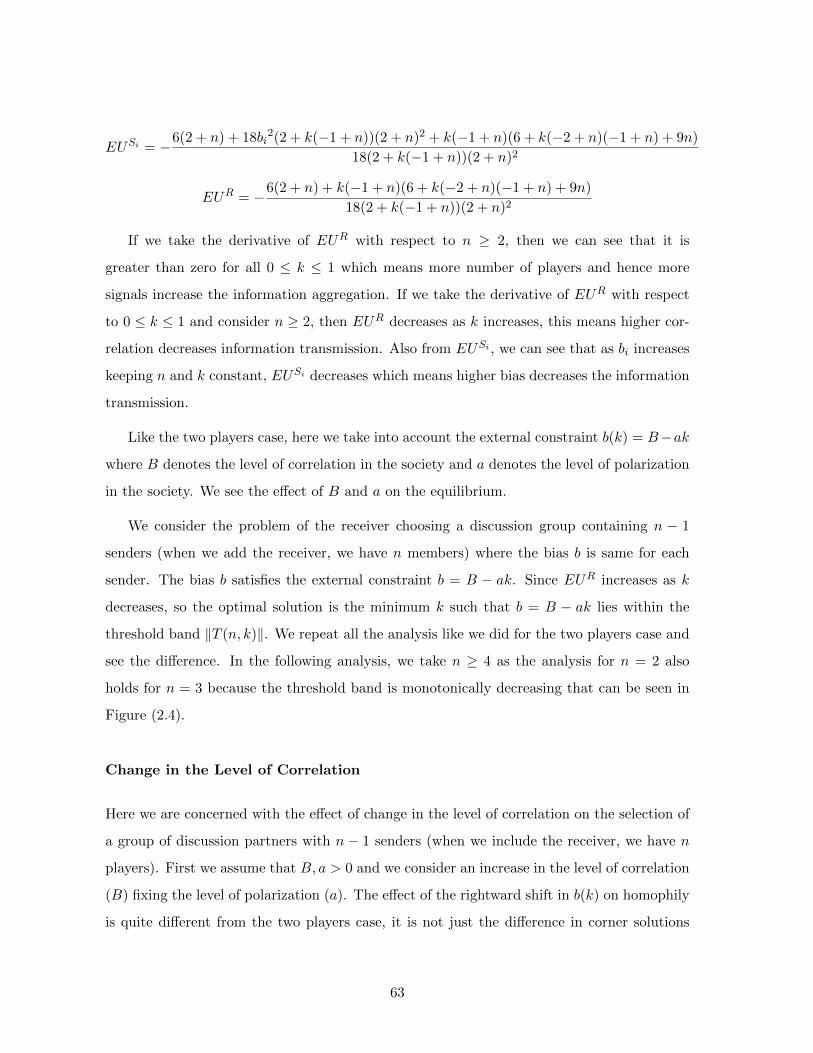
EUSi = −6(2 + n) + 18bi2(2 + k(−1 + n))(2 + n)2 + k(−1 + n)(6 + k(−2 + n)(−1 + n) + 9n)

18(2 + k(−1 + n))(2 + n)2

EUR = −6(2 + n) + k(−1 + n)(6 + k(−2 + n)(−1 + n) + 9n)

18(2 + k(−1 + n))(2 + n)2

If we take the derivative of EUR with respect to n ≥ 2, then we can see that it is

greater than zero for all 0 ≤ k ≤ 1 which means more number of players and hence more

signals increase the information aggregation. If we take the derivative of EUR with respect

to 0 ≤ k ≤ 1 and consider n ≥ 2, then EUR decreases as k increases, this means higher cor-

relation decreases information transmission. Also from EUSi , we can see that as bi increases

keeping n and k constant, EUSi decreases which means higher bias decreases the information

transmission.

Like the two players case, here we take into account the external constraint b(k) = B−ak

where B denotes the level of correlation in the society and a denotes the level of polarization

in the society. We see the effect of B and a on the equilibrium.

We consider the problem of the receiver choosing a discussion group containing n − 1

senders (when we add the receiver, we have n members) where the bias b is same for each

sender. The bias b satisfies the external constraint b = B − ak. Since EUR increases as k

decreases, so the optimal solution is the minimum k such that b = B − ak lies within the

threshold band ‖T (n, k)‖. We repeat all the analysis like we did for the two players case and

see the difference. In the following analysis, we take n ≥ 4 as the analysis for n = 2 also

holds for n = 3 because the threshold band is monotonically decreasing that can be seen in

Figure (2.4).

Change in the Level of Correlation

Here we are concerned with the effect of change in the level of correlation on the selection of

a group of discussion partners with n − 1 senders (when we include the receiver, we have n

players). First we assume that B, a > 0 and we consider an increase in the level of correlation

(B) fixing the level of polarization (a). The effect of the rightward shift in b(k) on homophily

is quite different from the two players case, it is not just the difference in corner solutions

63

and interior solutions because the threshold band is not monotonically decreasing as has been

shown in Figure (2.5).

k

Threshold for

Parallel shift

bn people

k(n)

B1

B2

B3

B5

B6

B4 O3

O2O1

kmin(n)

Slope = −a

O

Figure 2.5: The effect of parallel shift of b(k) = B − ak with B, a > 0 for n ≥ 4

Let’s consider the line B1− ak where B1 is less than b = −T (n, 0) (the positive threshold

at k = 0). The optimal solution is at (b, k) = (B1, 0). As we move rightward, B1 moves to

B2 which is within the threshold and the new optimal point is (B2, 0). So the homophily

decreases (the bias increases) as long as we have corner solution like the two players case. Now

consider the line B3− ak and a generalized increase in the correlation (rightward shift). The

optimal point is at O1 and as we move rightward, the optimal points move along the positive

threshold line which can be seen with the points O, O1, O2 and O3 in the Figure (2.5). We can

also notice that the correlation of the optimal points can not exceed the critical value kmin(n)

where the threshold attains the minimum value. The effect of rightward shift is as follows: if

the k-coordinate of the interior solution is smaller than kmin(n), then homophily increases and

if the k-coordinate of the interior solution is greater than kmin(n), then homophily decreases.

We can take B, a < 0 (where −B is the level of correlation and −a is the level of polariza-

tion) and the same implications hold while considering an increase in the level of correlation,

here we need to consider the threshold in the negative axis.

An important thing that can be observed from the above analysis that the difference from

the two players case arises because of the critical point kmin(n). When the correlation of the

optimal solution is smaller than kmin(n), then the same analysis like two players hold and the

difference arises when the correlation of the optimal solution is greater than kmin(n). The

conclusions of the above analysis is stated in the following proposition (we consider small

64

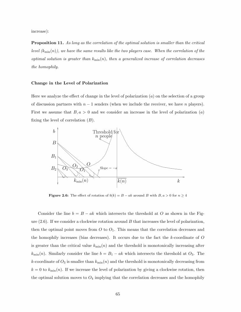
increase):

Proposition 11. As long as the correlation of the optimal solution is smaller than the critical

level (kmin(n)), we have the same results like the two players case. When the correlation of the

optimal solution is greater than kmin(n), then a generalized increase of correlation decreases

the homophily.

Change in the Level of Polarization

Here we analyze the effect of change in the level of polarization (a) on the selection of a group

of discussion partners with n− 1 senders (when we include the receiver, we have n players).

First we assume that B, a > 0 and we consider an increase in the level of polarization (a)

fixing the level of correlation (B).

k

Threshold forbn people

kmin(n)

B

OSlope = −aO1

k(n)

B2

B1

O2O3

Figure 2.6: The effect of rotation of b(k) = B − ak around B with B, a > 0 for n ≥ 4

Consider the line b = B − ak which intersects the threshold at O as shown in the Fig-

ure (2.6). If we consider a clockwise rotation around B that increases the level of polarization,

then the optimal point moves from O to O1. This means that the correlation decreases and

the homophily increases (bias decreases). It occurs due to the fact the k-coordinate of O

is greater than the critical value kmin(n) and the threshold is monotonically increasing after

kmin(n). Similarly consider the line b = B1 − ak which intersects the threshold at O3. The

k-coordinate of O3 is smaller than kmin(n) and the threshold is monotonically decreasing from

k = 0 to kmin(n). If we increase the level of polarization by giving a clockwise rotation, then

the optimal solution moves to O4 implying that the correlation decreases and the homophily

65

decreases. If we consider the line B2 − ak, a small increase in the level of polarization does

not change the optimal solution (B2, 0).

If we consider B, a < 0 (here −B is the level of correlation and −a is the level of po-

larization), then the above implications hold (we need to analyze with the threshold in the

negative axis).

As has been noted before, the difference from the two players case arises when the cor-

relation of the optimal solution is greater than kmin(n). All the above discussions can be

summarized in the following proposition (we consider small increase):

Proposition 12. As long as the correlation of the optimal solution is smaller than the critical

level (kmin(n)), we have the same results like the two players case. When the correlation of

the optimal solution is greater than kmin(n), then an increase in the level of polarization

decreases the homophily.

Change in the Levels of Correlation and Polarization

Above we studied a change in the level of correlation (B) keeping the level of polarization

fixed (a) and vice versa. Here we study the effect of simultaneous changes in both the level

of correlation and the level of polarization in the society.

Let’s assume that B, a > 0 and consider a rotation of the line b(k) = B − ak where a

increases. We explain the effect of rotation with the help of figures in Figure (2.7). Consider

the top figure where the line B−ak intersects the threshold at point O (the optimal solution)

and the k-coordinate of O is greater than kmin(n). If we make a clockwise rotation around

the point L1 lying below the threshold level, then we can see that the optimal point shifts

to O1. This means there is an increase in the correlation and a decrease in the homophily.

If we remember the analysis for two players case, this happens because we can decompose

the rotation around L1 into rotation around O (substitution effect) which increases the level

of polarization and then a rightward shift (income effect) which decreases the homophily.

Consider the bottom figure in Figure (2.7) and take a clockwise rotation around L2. Then

the optimal point moves from O to O2 which means homophily increases and correlation

decreases. This is because the rotation around L2 can be decomposed into a rotation aroundO

that increases the level of polarization and then a leftward shift that increases the homophily.

66

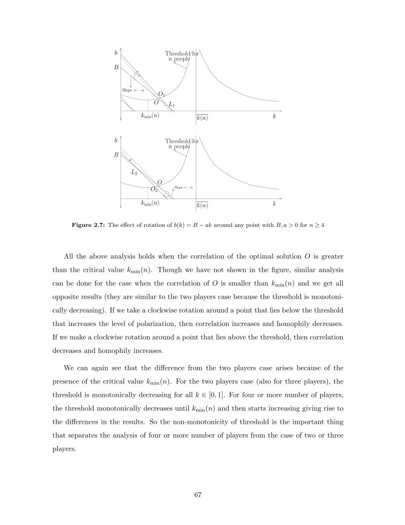
k

Threshold forbn people

k(n)kmin(n)

B

L1

O1Slope = −a

O

k

Threshold forbn people

k(n)kmin(n)

B

L2

OSlope = −aO2

Figure 2.7: The effect of rotation of b(k) = B − ak around any point with B, a > 0 for n ≥ 4

All the above analysis holds when the correlation of the optimal solution O is greater

than the critical value kmin(n). Though we have not shown in the figure, similar analysis

can be done for the case when the correlation of O is smaller than kmin(n) and we get all

opposite results (they are similar to the two players case because the threshold is monotoni-

cally decreasing). If we take a clockwise rotation around a point that lies below the threshold

that increases the level of polarization, then correlation increases and homophily decreases.

If we make a clockwise rotation around a point that lies above the threshold, then correlation

decreases and homophily increases.

We can again see that the difference from the two players case arises because of the

presence of the critical value kmin(n). For the two players case (also for three players), the

threshold is monotonically decreasing for all k ∈ [0, 1]. For four or more number of players,

the threshold monotonically decreases until kmin(n) and then starts increasing giving rise to

the differences in the results. So the non-monotonicity of threshold is the important thing

that separates the analysis of four or more number of players from the case of two or three

players.

67

2.4 Conclusion

We presented a Cheap Talk model where the signals of the senders and the receiver are

correlated. We first presented a basic model of two players and we showed that the threshold

for truth telling is decreasing in correlation. We extended the model to any number of players

and showed that the threshold of bias is non-monotonic as the correlation increases. We

imposed the external constraint where high correlation comes with low bias and analyzed the

selection of discussion partners (senders). We show that the non-monotonicity of threshold

separates the analysis of four or more number of players from the case of two or three players.

In the model of any number of senders, we focused the problem of the receiver selecting

a fixed number of senders. But it may be that choosing a group of few senders with less

correlation may be better than choosing a group with many senders and high correlation

i.e. there is a trade-off between n and k. Our next research will focus on this trade-off and

choosing the optimal discussion group.

2.5 Appendix

To show that k =cov(si,sj)σsiσsj

:

cov(si, sj) = E[(si − E(si))(sj − E(sj))] and σsi =√

var(si) =√E[(si − E(si))2] and

similarly, σsj =√

var(sj) =√E[(sj − E(sj))2].

E(si) = P (0|θ)× 0 + P (1|θ)× 1 = θ. σsi =√

(0− E(si))2P (0|θ) + (1− E(si))2P (1|θ) =√θ(1− θ) and similarly σsj =

√θ(1− θ).

cov(si, sj) = E[(si − E(si))(sj − E(sj))]

= P (0, 0|θ)(0− E(si))(0− E(sj)) + P (1, 0|θ)(1− E(si))(0− E(sj))

+P (0, 1|θ)(0− E(si))(1− E(sj)) + P (1, 1|θ)(1− E(si))(1− E(sj)) = kθ(1− θ)

Therefore, we can see that k =cov(si,sj)σsiσsj

holds true.

Derivation of f(θ|si, sj) and ysi,sj :

f(θ|si = 0, sj = 0) =P (si = 0, sj = 0|θ) f(θ)∫ 1

0 P (si = 0, sj = 0|θ) f(θ) dθ=

6

2 + k[(1− θ)2 + θ(1− θ)k]

68

Similarly, we can calculate that,

f(θ|si = 1, sj = 1) = 62+k [θ2 + θ(1− θ)k]

f(θ|si = 0, sj = 1) = 6 θ(1− θ) = f(θ|si = 1, sj = 0)

y00 =

∫ 1

0θf(θ|si = 0, sj = 0) dθ =

∫ 1

0

θ 6

2 + k[(1− θ)2 + θ(1− θ)k] dθ =

1 + k

2(2 + k)

Similarly we can calculate,

y01 =1

2= y10, y11 =

3 + k

2(2 + k)

Proof of Lemma (7):

Let sn−l be n− l number of zeros. Then

P (sn−l|θ) =∑

sl∈{0,1}lP (sl, sn−l|θ) = P (n 0s) +

l−1∑j=0

P (n− l 0s, (j 0s, l − j 1s))

= (1− θ)n(1− k) + (1− θ)k + (1− k)(1− θ)n−ll−1∑j=0

(1− θ)jθl−j

= (1− θ)k + (1− k)(1− θ)n−l

Similarly if sn−l be n− l number of ones, we can show that P (sn−l|θ) = θk + (1− k)θn−l.

Let sn−l be n− l − q number of zeros and q number of ones where q > 0. Then,

P (sn−l|θ) =∑

sl∈{0,1}lP (sl, sn−l|θ)

= (1− θ)n−l−qθq(1− k)l∑

j=0

(1− θ)jθl−j = (1− k)(1− θ)n−l−qθq

Proof of Theorem (9):

We can proceed in the same way like equation (2.2) for the two players case and the

indifference condition for n players become,∑s−i∈{0,1}n−1

P (s−i|si)42(s−i|si)

2≥ bi

∑s−i∈{0,1}n−1

4(s−i|si)P (s−i|si) (2.12)

where 4(s−i|si) = y1−si,s−i− ysi,s−i

.

4(s−i|si) = −4(s−i|1− si) (2.13)

69

As P (si) =1

2, P (s−i|si) =

P (s−i, si)

P (si)= 2P (s−i, si) (2.14)

P (0, 0, ..., 0) =2 + k(n− 1)

2(n+ 1)= P (1, 1, ..., 1) (2.15)

P (l(1s), (n− l)(0s)) =(1− k)(n− l)! l!

(n+ 1)!= P (l(0s), (n− l)(1s)) (l 6= 0, n− 1) (2.16)

From the computation which is given afterwards when we compute the explicit limit of bi,

we have

4(0, ..., 0|0) = 4(1, ..., 1|0) (2.17)

4(l(1s), (n− 1− l)(0s)|0) =−1

2 + n(l 6= 0, n− 1) (2.18)

From, (2.13),(2.14),(2.15),(2.16),(2.17),(2.18) we have,∑s−i∈{0,1}n−1

P (s−i|si)42(s−i|si)

2=

∑s−i∈{0,1}n−1

P (s−i|1− si)42(s−i|1− si)

2(2.19)

∑s−i∈{0,1}n−1

4(s−i|si)P (s−i|si) = −∑

s−i∈{0,1}n−1

4(s−i|1− si)P (s−i|1− si) (2.20)

Consider∑

s−i∈{0,1}n−14(s−i|si)P (s−i|si) which is a function of n and k. If for a partic-

ular combination of n and k,∑

s−i∈{0,1}n−14(s−i|si)P (s−i|si) = 0 (iff it is true for si = 0,

then also true for si = 1 from (2.20)), then the player is indifferent between telling 0 and 1

whether he has signal 0 or 1 by (2.12) and the fact that∑

s−i∈{0,1}n−1 P (s−i|si)42(s−i|si)

2 > 0.

So let’s consider n and k such that∑

s−i∈{0,1}n−14(s−i|si)P (s−i|si) 6= 0. It is always true

that∑

s−i∈{0,1}n−1 P (s−i|si)42(s−i|si)

2 > 0. Since (2.20) holds, from (2.12), the condition for

truth telling is given by,

‖bi‖ ≤ ‖∑

s−i∈{0,1}n−1 P (s−i|si)42(s−i|si)

2∑s−i∈{0,1}n−14(s−i|si)P (s−i|si)

‖

Calculation of the explicit value of the limit of bi :

y1,1,...,1 =2(n+ 1)(3− k + kn)

3(n+ 2)(2− k + kn), y0,0,...,0 =

6 + k(n− 1)(n+ 4)

3(n+ 2)(2− k + kn), yl(1s),(n−l)(0s) =

1 + l

n+ 2

4(0, ..., 0|0) =6− k(2− 3n+ n2)

3(2 + k(−1 + n))(2 + n)= 4(1, ..., 1|0)

.

4(l(1s), (n− 1− l)(0s)|0) =−1

2 + n(l 6= 0, n− 1)

70

We can see that, 4(s−i|si) = −4(s−i|1− si) and hence we have,

4(0, ..., 0|1) = −4(0, ..., 0|0) = 4(1, ..., 1|1)

4(l(1s), (n− 1− l)(0s)|1) = −4(l(1s), (n− 1− l)(0s)|0) (l 6= 0, n− 1)

Let’s denote,41(si) = 4(0, ..., 0|si) = 4(1, ..., 1|si)

42(si) = 4(l(1s), (n− 1− l)(0s)|si) (l 6= 0, n− 1)

Also as P (si) = 12 , P (s−i|si) = P (s−i,si)

P (si)= 2P (s−i, si).

P (0, 0, ..., 0) =2 + k(n− 1)

2(n+ 1)= P (1, 1, ..., 1)

P (l(1s), (n− l)(0s)) =(1− k)(n− l)! l!

(n+ 1)!= P (l(0s), (n− l)(1s))

And if we know, P (0, ..., 0|si) and P (1, ..., 1|si) then

l=n−2∑l=1

P (l(1s), (n− 1− l)(0s)|si) = 1− P (0, ..., 0|si)− P (1, ..., 1|si)

= 1− 2P (si, 0, ..., 0)− 2P (si, 1, ..., 1)

If we denote P (si, 0, ..., 0) + P (si, 1, ..., 1) = P ∗, we can see that P ∗ is same for si = 0, 1.

So we can write,

∑s−i∈{0,1}n−1

4(s−i|si)P (s−i|si) = 41(si)2P∗ +42(si)(1− 2P ∗)

= −[41(1− si)(2P ∗) +42(1− si)(1− 2P ∗)] (2.21)

∑s−i∈{0,1}n−1

P (s−i|si)42(s−i|si)

2=42

1(si)

22P ∗ +

422(si)

2(1− 2P ∗)

=42

1(1− si)2

2P ∗ +42

2(1− si)2

(1− 2P ∗) (2.22)

Let T (n, k) =

∑s−i∈{0,1}n−1 P (s−i|0)4

2(s−i|0)2∑

s−i∈{0,1}n−14(s−i|0)P (s−i|0)

Using above computations we can calculate that,

T (n, k) = −36n+ k(−2 + n)(−1 + n)(12 + k(−17 + k(−5 + n)(−1 + n)(1 + n) + n(−9 + 2n)))

6(2 + k(−1 + n))(2 + n)(−6n+ k(−2 + n)(−1 + n)(−1 + k + kn))

71

.

When Si observes si = 0, from equation (2.12), if T (n, k) ≥ 0, the threshold for truth

telling is given by, bi ≤ T (n, k) and if T (n, k) ≤ 0, then bi ≥ T (n, k).

When Si observes si = 1, from equation (2.12), (2.19) and (2.20), if T (n, k) ≥ 0, the

threshold for truth telling is given by, bi ≥ −T (n, k) and if T (n, k) ≤ 0, then bi ≤ −T (n, k).

Using all the above computations, we have the limit of bi which is given by,

‖bi‖ ≤ ‖T (n, k)‖

Proof of Proposition (10):

As the first bracket of the denominator in equation (2.10), 6(2+k(−1+n))(2+n) > 0, we

need to see whether the second bracket of the denominator −6n+ k(−2 + n)(−1 + n)(−1 +

k+ kn) = 0 which is a quadratic equation in k. We’ll consider n ≥ 3 as for n = 1, n = 2, the

above term is always negative. After factorizing we have,

(k − (n−1)(n−2)+√

(n−1)2(n−2)2+4.6n.(n−2)(n−1)(1+n)

2(n−2)(n−1)(1+n) )

(k − (n−1)(n−2)−√

(n−1)2(n−2)2+4.6n.(n−2)(n−1)(1+n)

2(n−2)(n−1)(1+n) ) = 0

⇒ k =(n−1)(n−2)−

√(n−1)2(n−2)2+4.6n.(n−2)(n−1)(1+n)

2(n−2)(n−1)(1+n) ,

k =(n−1)(n−2)+

√(n−1)2(n−2)2+4.6n.(n−2)(n−1)(1+n)

2(n−2)(n−1)(1+n)

Since 0 ≤ k ≤ 1 and

(n− 1)(n− 2)−√

(n− 1)2(n− 2)2 + 4.6n.(n− 2)(n− 1)(1 + n)

2(n− 2)(n− 1)(1 + n)< 0,

the relation k =(n−1)(n−2)−

√(n−1)2(n−2)2+4.6n.(n−2)(n−1)(1+n)

2(n−2)(n−1)(1+n) is not satisfied.

So the only relation that we consider is,

k =(n− 1)(n− 2) +

√(n− 1)2(n− 2)2 + 4.6n.(n− 2)(n− 1)(1 + n)

2(n− 2)(n− 1)(1 + n)(2.23)

For n = 3, the right hand side is strictly greater than 1, so we have the upper limit of bi

for all 0 ≤ k ≤ 1. For n = 4, the right hand side is equal to 1 and the upper limit of bi is

unbounded for k = 1. As n increases further from n = 4, k decreases. For all n ≥ 4, there

exists a k ∈ [0, 1], where bi does not have an upper limit.

Chapter 3

Information Transmission under

Leakage

Abstract: This chapter1 analyzes the effect of information leakage on strategic communi-

cation for example in discussion groups. A sender transmits the information to a first-hand

receiver who instead of taking the decision (due to time, legal or other constraints), leaks the

information to a second-hand receiver in his circle of trust who in turn takes the decision.

If the first-hand receiver takes the decision herself without transmitting the information, we

say that there is non-leakage of information. We consider a binary signals framework and

define the total flow of the information in the society as the set of first-hand and second-hand

receivers that can possibly receive true signals in the truth telling equilibrium. We show

that for centrist senders, total flow of information is double under leakage; for moderate and

extremist senders, it is less than double. We compare the welfare of the society under leakage

and under non-leakage We show that when the first-hand receiver’s preference is close (if

far) to the mean preference of the society, non-leakage (then leakage) is better. We further

show that cardinality of the first-hand receivers where non-leakage is preferred is a concave

function of the homogeneity.

JEL Code : C72, D82, D83

Keywords : Cheap Talk, Leakage

1A joint work with Giovanni Ursino, Catholic University of Milan

73

3.1 Introduction

In practical situations where the sender (expert) advises the receiver (decision maker), the

sender needs to take into account that the receiver may not be taking the decision herself due

to some constraints like unavailability of time, legal or financial constraints and she passes

the information to one of her associates in her circle of trust who takes the decision. These

phenomena can be observed in on-line discussion forums, in lobbying groups and in debates.

We call the receiver who gets direct information from the sender as ’first-hand receiver’ and

the associate who gets information from the first-hand receiver as ’second-hand receiver’.

So the sender has to consider the fact that the information that he transmits to the first-

hand receiver may get leaked to second-hand receiver who in turn takes the decision. In this

paper we consider a strategic communication (Cheap Talk) model that takes into account the

leakage of information where the sender, the first-hand and second-hand receivers all differ

in their preferences (biases).

The first-hand receiver acts as a strategic mediator like Ivanov (2010) [15] who passes the

information to second-hand receiver. Since the preferences of the sender is different from the

first-hand receiver, the preference of the first-hand receiver is different from the second-hand

receiver (there is bias among the preferences), the information may not transmit perfectly as

in each stage of communication, the conflicts of the players comes into play. In our framework,

we consider that the first-hand receiver assigns the decision randomly to one the associates

within her circle of trust (whom she can send informative signals). This is because all the

players in her circle of trust may not be available always, or she may not want to meet just

a fixed associate and so she assigns the decision whomever she meets in the circle of trust

(ideally she would have preferred to take the action by herself).

Some of the interesting questions in our framework are: what is the limit on the biases of

the first-hand receivers and second-hand receivers so that they get informative signals, does

leaking the information increases the welfare of the society than not leaking (the first-hand

receiver takes the decision herself), what is the role of homogeneity on leakage etc.

The papers of Ivanov (2010) [15] and Ambrus et al. (2012) [3] discuss the role of strategic

mediator and the role of biases on information transmission in detail. But the issues we

consider are complicated to answer in their framework because they consider that the sender

74

knows the exact state θ which leads to partition intervals like Crawford and Sobel (1982)

[7] which introduces difficulty into analysis. To have a simplified analysis, we adopt the

binary signals framework as discussed in Morgan and Stocken (2008) [20] in the context of

information aggregation in polls and it has been used later by Galeotti et al. (2011) [10] to

discuss Cheap Talk in networks. In the binary signals framework, the sender does not receive

the exact state of the world θ, rather an imperfect signal which takes the value either 0 or

1 about the state of the world θ. This keeps our model simpler than Ivanov (2010) [15] and

Ambrus et al. (2012) [3]. We consider a continuum of players lying on the unit interval [0, 1]

and whose biases vary continuously on the closed interval [0, b] where b measures how the

bias vary across agents. The number 1b can be used an index for the homogeneity because a

higher b means the preference vary a lot in the society and so the homogeneity is less in the

society. Like Galeotti et al. (2011) [10], we consider equilibrium with truthful communication

(pure strategies) because all the information is transmitted in this equilibrium. Since we are

considering sequential game with incomplete information, the natural choice of equilibrium

in our framework is Perfect Bayesian Nash Equilibrium (PBNE).

While finding the equilibria, we first consider the sub-game where the first-hand receiver

communicates with the second-hand receiver and we find the threshold on the difference in

biases for truth telling. The second-hand receivers whose biases lie in the threshold of truth

telling are called “circle of trust”. We can see that the circle of trust for a first-hand receiver

is independent of the sender who sends signals. Then we consider the sender who takes into

account that the first-hand receiver may leak the information to others in her circle of trust

and we find the threshold on the difference in biases between the sender and the first-hand

receiver for truth telling. Combining both the limits of each stage, we can answer if leakage

spreads the information than non-leakage. We show that the total flow of information (which

is measured in terms of the set of first-hand and second-hand receivers that can possibly get

true signals in the equilibrium) increases when there is leakage. The total flow of information

is higher for senders with centrist preference and it decreases as the sender gradually becomes

extremist. Then we compare the total welfare of the society under leakage and non-leakage so

that the policy makers can decide whether to act to relax the constraint so that the first-hand

receivers take actions themselves. We demonstrate that leakage is better for the society if

the bias of the first-hand receiver lies close to the boundary on the preference interval [0, b]

and non-leakage is better for the society if the bias of the first-hand receiver lies close to the

75

center of [0, b]. We also study the impact of homogeneity 1b on leakage versus non-leakage.

3.2 Model of Information Leakage

There is a continuum of agents uniformly distributed on the unit interval [0, 1]. The agents

are denoted by i which also corresponds to their position on the unit interval. The state of the

world is θ is uniformly distributed over the state space Θ = [0, 1]. One of the agents, that we

denote as sender is, receives an informative signal s about the state θ, with P (s = 1|θ) = θ.

After receiving the signal, is meets one agent randomly in the economy and we denote this

agent as ir1 . Sender is sends a message ms : {0, 1} → {0, 1} to ir1 . We refer to this message

as “first-hand” information and agent ir1 as the “first-hand” receiver. After receiving the

message ms, agent ir1 randomly meets other agents in the economy, but only those to whom

he could send informative signals2 and we denote this randomly met agent as ir2 . Receiver

ir1 sends a message mr1 : {0, 1} → {0, 1} to ir2 . We refer to this message as “second-hand”

information and agent ir2 as the “second-hand” receiver. After all information is transmitted,

agent ir2 takes action y. The preference (bias) of the agent i is given by b · i where b > 0

denotes the proportional change in the bias across the agents. As describe in the introduction,

1b measures the homogeneity in the society. The preferences of is, ir1 and ir2 are b · is, b · ir1and b · ir2 respectively.

The quadratic loss utility function of agent i is given by:

U(y, θ, i) = −(y − θ − b · i)2

Note that each agent i is characterized by the “bliss point” θ + b · i which maximizes his

utility.

We associate with this economy the following sequential game.

At time 1, agent is receives a signal s and decides a message ms for agent ir1 that he

meets randomly. At time 2, ir1 meets ir2 randomly among the group of agents to whom ir1

can communicate informative signals (in his circle of trust), and a message mr1 is chosen by

ir1 for agent ir2 . At time 3, agent ir2 takes an action y.

2We can take this assumption because once ir1 receives a message from is, the choice of ir2 does not depend

on the previous stage, so ir1 meets randomly to only those with whom she can communicate truthfully.

76

The natural choice of the equilibrium for the sequential game with incomplete information

is Perfect Bayesian Nash Equilibrium (PBNE). Let in the equilibrium, the signaling strategy

of is be qs(ms|s), the signaling strategy of ir1 be qr1(mr1 |ms) and the action of ir2 be y(mr2).

Let µ(θ|ms) be the belief of ir1 about the state θ after hearing the message ms and ρ(θ|mr1)

be the belief of ir2 about the state θ after hearing the message mr1 . The PBNE is defined as:

Given the equilibrium strategies of other players, 1) y(mr2) maximizes agent ir2 ’s expected

utility where the belief µ(θ|mr1) is obtained by Bayes’ rule on the equilibrium path; 2) The

message mr1 in the support of qr1(.|ms) maximizes the expected utility of agent ir1 where

the belief ρ(θ|ms) is obtained by Bayes’ rule on the equilibrium path; 3) The message ms in

the support of qs(.|s) maximizes the expected utility of agent is 4) The out of equilibrium

path beliefs should be such that deviation is not profitable.

A truth telling equilibrium of this game is one where qs(ms = s|s) = 1 and qr1(mr1 =

ms|ms) = 1 for all s and all ms. We first note that in the truth telling equilibrium, there are

no out of equilibrium paths. We study the game by backward induction, starting from the

problem faced by any agent ir2 which receives information from the first-hand receiver ir1 .

3.3 Truth Telling Equilibrium

Let us first consider the problem faced by the receiver of first-hand information ir1 . Our

aim is to derive conditions for the truth telling message mr1 . Naturally, this problem is

meaningful only when ms is itself a truth telling strategy. Otherwise, equilibrium would

require that the second-hand receiver gives no informational value to the received message.

Therefore we consider s = ms = mr1 in the truth telling equilibrium. As it is well known,

conditions for truth telling bear on the distance in the preferences of the first-hand receiver

ir1 and the agent ir2 to which ir1 discloses the message ms received by the sender is.

y(mr1) = arg maxy−∫ 1

0(y − θ − b · ir2)2 f(θ|mr1) dθ

The optimal solution is given by:

y(mr1) = E(θ|mr1) + b · ir2

Since s = ms = mr1 in the truth telling equilibrium,

y(mr1) = y(s) = E(θ|s) + b · ir2

77

Since θ is uniformly distributed over [0, 1] we have,

f(θ|1) = 2θ, f(θ|0) = 2(1− θ); and so y(1) =2

3+ b · ir2 , y(0) =

1

3+ b · ir2

We now derive the truth telling interval for the first-hand receiver. The incentive condition

for ir1 to tell the true message mr1 = ms = s to agent ir2 is given by:

−∫ 1

0(y(s)− θ − b · ir1)2 f(θ|s) dθ ≥ −

∫ 1

0(y(1− s)− θ − b · ir1)2 f(θ|s) dθ

⇒ −(y(s)− E(θ|s)− b · ir1)2 ≥ −(y(1− s)− E(θ|s)− b · ir1)2

⇒ −(E(θ|s) + b · ir2 − E(θ|s)− b · ir1)2 ≥ −(E(θ|1− s) + b · ir2 − E(θ|s)− b · ir1)2

⇒ (E(θ|s)− E(θ|1− s))2 ≥ 2(b · ir2 − b · ir1)(E(θ|s)− E(θ|1− s))

Here, E(θ|s) − E(θ|1 − s) = 1/3 for s = 1 and −1/3 for s = 0 and we know b > 0. So the

above incentive condition becomes,

|ir2 − ir1 | ≤1

6b(3.1)

When considering the sender’s problem, we need to account for the possibility that for some

first-hand receiver ir1 , the truth telling interval exceeds the boundaries of the admissible

agents’ labels [0, 1]. Let us then denote by [l(ir1), r(ir1)] or in short [l, r] the interval (possibly

constrained) for a given receiver ir1 . We denote as unconstrained the case in which [l, r] has

length 26b where 0 ≤ l = ir1 − 1

6b and r = ir1 + 16b ≤ 1. Constrained cases are when either

ir1− 16b < 0 and r = ir1 + 1

6b ≤ 1 (in which case l = 0, denoted as l-constrained) or ir1 + 16b > 1

and 0 ≤ l = ir1− 16b (in which case r = 1, denoted as r-constrained ) or when both ir1− 1

6b < 0

and ir1 + 16b > 1 (in which case l = 0 and r = 1, denoted as lr-constrained). Summarizing

we have l = max[0, i− 1

6b

]and r = min

[i+ 1

6b , 1]. For sender is, the incentive condition to

report the true signal s to ir1 is given by,∫ r

l

(∫ 1

0−(yir2 (s)− θ − b · is)2f(θ|s)dθ

)dir2

≥∫ r

l

(∫ 1

0−(yir2 (1− s)− θ − b · is)2f(θ|s)dθ

)dir2

78

⇒∫ r

l−(yir2 (s)− E(θ|s)− b · is)2dir2 ≥

∫ r

l−(yir2 (1− s)− E(θ|s)− b · is)2dir2

⇒∫ r

l−(E(θ|s) + b · ir2 − E(θ|s)− b · is)2 + (E(θ|1− s) + b · ir2 − E(θ|s)− b · is)2dir2 ≥ 0

⇒∫ r

l(E(θ|1− s)− E(θ|s))2 + 2(b · ir2 − b · is)(E(θ|1− s)− E(θ|s)) dir2 ≥ 0

⇒ (E(θ|s)− E(θ|1− s))2 ≥ 2(b · r + l

2− b · is)(E(θ|s)− E(θ|1− s))

Since E(θ|0) = 13 ,E(θ|1) = 2

3 and b > 0, we have for s = 1, l+r2 − is ≤

16b and for s = 0,

l+r2 − is ≥ −

16b . Combining both these conditions, we have for truth telling,∣∣∣∣ l + r

2− is

∣∣∣∣ ≤ 1

6b(3.2)

The above inequality has the following meaning: if ir1 is talking to other agents then, for

truth telling the thing that matters is the distance between is and the average index of the

agents that ir1 talks to and the homogeneity 1b in the society.

CASE Range of ir1 s s = 0 s = 1

unconstrained ir1 ∈(

16b , 1−

16b

)|ir1 − is| < 1

6b ir1 − is >

− 16b

ir1− is < 16b

l-constrained ir1 <16b <

12

∣∣∣ ir1+ 16b

2 − is∣∣∣ < 1

6b ir1 − is >

is − 36b

ir1 − is <

is + 16b

r-constrained ir1 > 1− 16b >

12

∣∣∣ ir1− 16b

+1

2 − is∣∣∣ < 1

6b ir1 − is >

is − 1− 16b

ir1 − is <

is − 1 + 36b

lr-constrained i ∈ [0, 1] , 16b >

12

∣∣12 − is

∣∣ < 16b is <

12 + 1

6b is >12 −

16b

Let the total flow of information be defined as the set of first-hand and second-hand

receivers that can possibly receive the true signal in the equilibrium. Consider 16b <

14 meaning

the homogeneity 1b is low in the society. Let the sender with preference in [ 2

6b , 1−26b ] be denoted

as ‘centrist’, the sender with preference in [ 16b ,

26b ] ∪ [1− 2

6b , 1−16b ] be denoted as ‘moderate’

and the sender with preference in [0, 16b ] ∪ [1− 1

6b , 1] be denoted as ‘extremist’ (figure (3.1)).

We have the following proposition that describes about the flow of the information in the

society.

Proposition 13. Consider 16b <

14 i.e. the homogeneity is low. Leakage never decreases

the amount of first-hand information, and always increases the total flow of information in

79

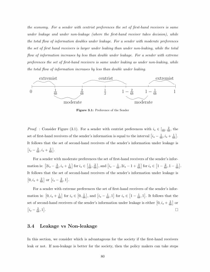
the economy. For a sender with centrist preferences the set of first-hand receivers is same

under leakage and under non-leakage (where the first-hand receiver takes decision), while

the total flow of information doubles under leakage. For a sender with moderate preferences

the set of first hand receivers is larger under leaking than under non-leaking, while the total

flow of information increases by less than double under leakage. For a sender with extreme

preferences the set of first-hand receivers is same under leaking as under non-leaking, while

the total flow of information increases by less than double under leaking.

extremist centrist extremist

moderate

0

moderate

11− 26b 1− 1

6b12

26b

16b

Figure 3.1: Preference of the Sender

Proof. : Consider Figure (3.1). For a sender with centrist preferences with is ∈ [6b ,26b , the

set of first-hand receivers of the sender’s information is equal to the interval[is − 1

6b , is + 16b

].

It follows that the set of second-hand receivers of the sender’s information under leakage is[is − 2

6b , is + 26b

].

For a sender with moderate preferences the set of first-hand receivers of the sender’s infor-

mation is:[2is − 3

6b , is + 16b

]for is ∈

[16b ,

26b

], and

[is − 1

6b , 2is − 1 + 36b

]for is ∈

[1− 2

6b , 1−16b

].

It follows that the set of second-hand receivers of the sender’s information under leakage is[0, is + 2

6b

]or[is − 2

6b , 1].

For a sender with extreme preferences the set of first-hand receivers of the sender’s infor-

mation is:[0, is + 1

6b

]for is ∈

[0, 1

6b

], and

[is − 1

6b , 1]

for is ∈[1− 1

6b , 1]. It follows that the

set of second-hand receivers of the sender’s information under leakage is either[0, is + 2

6b

]or[

is − 26b , 1

].

3.4 Leakage vs Non-leakage

In this section, we consider which is advantageous for the society if the first-hand receivers

leak or not. If non-leakage is better for the society, then the policy makers can take steps

80

to relax the constraint that makes it difficult for the first-hand receivers to take the actions

themselves. We also study the role of the homogeneity 1b on leakage versus non-leakage.

3.4.1 A Fixed First-hand Receiver

As a first step to analyze leakage vs non-leakage, we change our model little bit and assume

that is meets a fixed ir1 to whom he can reveal truthfully and study the effect of leakage. Then

using it as a base, we extend it to the case where is meets ir1 randomly. Under non-leakage

only ir1 receives information and takes action herself as she does not assign the decision to

any of her associates. Under leakage, ir1 transmits the information randomly to one of her

associates in her circle of trust who then takes the decision. We analyze if leakage helps

more information transmission in the society which is measured in terms of ex-ante expected

utility.

The ex-ante expected utility of the society under leakage is given by (index i represents

anybody in the society):

EU(leakage) =∑

s∈{0,1}

P (s)

∫ 1

0

(∫ r

l

[∫ 1

0−(yir2 (s)− θ − b · i)2 f(θ|s) dθ

]1

r − ldir2

)di

= −b2

3

[(r2 + l2 + rl) + 1− 3

2(r + l)

]

The ex-ante expected utility under non-leakage is given by (index i represents anybody

in the society):

EU(non− leakage) =∑

s∈{0,1}

P (s)

∫ 1

0

[∫ 1

0−(yir1 (s)− θ − b · i)2 f(θ|s) dθ

]di

= −b2

3

[3i2r1 + 1− 3ir1

]Leakage is better than non-leakage if

− b2

3

[(r2 + l2 + rl) + 1− 3

2(r + l)

]≥ −b

2

3

[3i2r1 + 1− 3ir1

]⇒ (r2 + l2 + rl) + 1− 3

2(r + l) ≤ 3i2r1 + 1− 3ir1

⇒ 3i2r1 − 3ir1 +3

2(r + l)− (r2 + l2 + rl) ≥ 0 (3.3)

To solve equation (3.3), we consider four cases that includes all possibilities which are:

81

1. l = ir1 − 16b , l 6= 0 and r = ir1 + 1

6b , r 6= 1

2. l = ir1 − 16b , l 6= 0 and r = 1

3. l = 0 and r = ir1 + 16b , r 6= 1

4. l = 0 and r = 1

We divide the domain of b into three intervals which are:

1. 0 < b ≤ 16 . Here for any ir1 ∈ [0, 1], l = 0 and r = 1.

2. 16 < b ≤ 1

3 . Here 16b ≥

12 . For ir1 ∈ [1 − 1

6b ,16b ], we have l = 0 and r = 1. For

ir1 ∈ [0, 1 − 16b), we have l = 0, r = ir1 + 1

6b . For ir1 ∈ ( 16b , 1], we have l = ir1 − 1

6b ,

r = 1.

3. b > 13 . Here 1

6b <12 . For ir1 ∈ ( 1

6b , 1 −16b), we have l = ir1 − 1

6b and r = ir1 + 16b . For

ir1 ∈ [0, 16b ], we have l = 0, r = ir1 + 1

6b . For ir1 ∈ [1− 16b , 1], we have l = ir1 − 1

6b , r = 1.

We considered various combinations of the above cases and Table (3.1) summarizes the

advantage of leakage or non-leakage for various combinations of b and ir1 . In the table and the

figure, YL = 2+9b24b −

√4−12b+27b2

b2

8√

3, ZH = −2+15b

24b +

√4−12b+27b2

b2

8√

3and A = [1

6(3−√

3), 16(3 +

√3)].

Table (3.1) and the proof for its construction is given in the appendix. Figure (3.2) graphically

illustrates the results of Table (3.1) and shows the intervals of ir1 comparing leakage and non-

leakage for various values of b.

The table and the figure are quite clear in their message: if the first-hand receiver lies

close to the center of the interval [0, b], then non-leakage is better and if it lies farther from

the center, then leakage is better. This is because for the society, the best is if the person who

takes decision is at the center so that the welfare loss due to bias is minimum. If the first-

hand receiver’s bias lies close to the center, then it is better for the society that she herself

takes the decision rather than assigning the decision to somebody else. But if the first-hand

receiver’s bias is far from the center, then it is better to leak that information to one of her

associates so that the associates having bias close to the center have a higher probability of

taking decisions thus benefiting the society. The following proposition summarizes the above

discussion.

82

l = ir1 − 16b , l 6=

0; r = ir1 +

16b , r 6= 1

l = ir1− 16b , l 6= 0;

r = 1

l = 0; r = ir1 +

16b , r 6= 1

l = 0; r = 1

b ≤ 16 non feasible non feasible non feasible non-leakage for

ir1 ∈ A; leakage

for [0, 1] \A16 < b ≤ 1

3 non feasible if 16 ≤ b ≤ 3−

√3

6

leakage for ir1 ∈

( 16b , 1]

if 16 ≤ b ≤ 3−

√3

6

leakage for ir1 ∈

[0, 1− 16b)

if 16 ≤ b ≤

3−√

36 leakage for

ir1 ∈ [1 − 16b ,

16b ] \

A; non-leakage for

ir1 ∈ A

if 3−√

36 ≤ b ≤ 1

3

leakage for

ir1 ∈ [ZH , 1];

non-leakage for

ir1 ∈ ( 16b , ZH ]

if 3−√

36 ≤ b ≤ 1

3

leakage for

ir1 ∈ [0, YL];

non-leakage for

ir1 ∈ [YL, 1− 16b)

if 3−√

36 ≤ b ≤

13 non-leakage for

ir1 ∈ [1− 16b ,

16b ]

b > 13 non-leakage for

ir1 ∈ ( 16b , 1−

16b)

leakage for

ir1 ∈ [ZH , 1];

non-leakage for

ir1 ∈ [1− 16b , ZH ]

leakage for

ir1 ∈ [0, YL];

non-leakage for

ir1 ∈ [YL,16b ]

non feasible

Table 3.1: Leakage vs Non-leakage for ir1

83

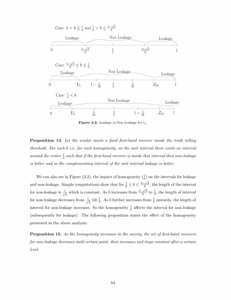
Leakage Non Leakage Leakage

Leakage Non LeakageLeakage

Leakage LeakageNon Leakage

3−√3

60 1

23+√3

6 1

12 11− 1

6b0

1− 16b 10

16b

16b

12

YL ZH

YL ZH

Case: 0 < b ≤ 16 and

16 < b ≤ 3−

√3

6

Case: 3−√3

6 ≤ b ≤ 13

Case: 13 < b

Figure 3.2: Leakage vs Non Leakage for ir1

Proposition 14. Let the sender meets a fixed first-hand receiver inside the truth telling

threshold. For each b i.e. for each homogeneity, on the unit interval there exists an interval

around the center 12 such that if the first-hand receiver is inside that interval then non-leakage

is better and in the complementary interval of the unit interval leakage is better.

We can also see in Figure (3.2), the impact of homogeneity (1b ) on the intervals for leakage

and non-leakage. Simple computations show that for 16 ≤ b ≤

3−√

36 , the length of the interval

for non-leakage is 1√3

which is constant. As b increases from 3−√

36 to 1

3 , the length of interval

for non-leakage decreases from 1√3

till 12 . As b further increases from 1

3 onwards, the length of

interval for non-leakage increases. So the homogeneity 1b affects the interval for non-leakage

(subsequently for leakage). The following proposition states the effect of the homogeneity

presented in the above analysis:

Proposition 15. As the homogeneity increases in the society, the set of first-hand receivers

for non-leakage decreases until certain point, then increases and stays constant after a certain

level.

84

3.4.2 Randomly Selected First-hand Receiver

In the previous section, we considered when iS meets a fixed ir1 . Now we allow is to randomly

meet ir1 as in our original model and we want to consider whether leakage is better for the

society than non-leakage. To have this analysis, the previous calculations provide a base.

Suppose we know the range of ir1 to whom iS communicates truthfully for a given b. We

can neglect the first-hand receivers who lie outside the truth telling interval of is because

if they leak or not leak, the action taken does not change because there is no information

transmission. So we can take the first-hand receivers ir1 inside the truth telling threshold of

iS and use Figure (3.2) for a given b to see whether ir1 lies within an interval where non-

leakage is better. If it happens so, then we can say that non-leakage is better for the society.

If it lies entirely within an interval where leakage is better, then for the society leakage is

better. These analysis clearly says that if is lies sufficiently close to the point 12 for b ≥ 3−

√3

6

(consult Figure (3.2)), then non-leakage is better because the first-hand receivers lie close to

the mean preference 12 which is better for the society. As the sender moves away from 1

2 , the

set of both first-hand receivers and the second-hand receivers move away also from the center

and hence leakage will be preferred. The following proposition summarizes these discussion:

Proposition 16. For 3−√

36 ≤ b i.e. for low homogeneity in the society, on the unit interval

there exists an interval around the center 12 such that if the sender is inside that interval,

then non-leakage is better and in the complementary interval of the unit interval leakage is

better.

The explicit calculation of the intervals of is where non-leakage is better and the role

of the homogeneity on the intervals of non-leakage and leakage are left for our future work.

However I mention how to proceed in that direction. We have already considered when the

set of first-hand receivers within the truth telling threshold of iS lie inside the interval where

leakage is better or inside the interval where non-leakage is better. The other case is if part of

the receivers lie in the interval where non-leakage is better and the other part in the interval

where leakage is better. In that case, we can employ the following method to see whether

leakage is better than non-leakage. Consider the part of the receivers in the interval where

leakage is better and calculate the utility loss of the society, if they do not leak. Similarly

calculate the utility loss of the society due to leakage for the part of the receivers in the

interval where non-leakage is better. Then compare these two utility losses. If the utility loss

85

due to leakage by the receivers in the interval where non-leakage is better, is more than the

utility loss due to non-leakage by the receivers in the interval where leakage is better, then

for the society non-leakage is better and for the opposite case leakage is better.

3.5 Conclusion

We considered a model of two stage communication in a binary signals framework with

truthful revelation in the equilibrium. We showed that the total flow of information in the

society is higher with leakage than non-leakage. Then we considered whether leakage is

better than non-leakage for the society so that policy makers can take steps to mitigate the

constraint that do not allow first-hand receivers to take actions themselves. We show that

non-leakage is better for the society if the sender lies close to the mean preference and leakage

is better if he lies far from the mean preference.

The future work can focus the study another phenomenon in discussion groups where

first-hand receivers not only meets people in her circle of trust, but anybody on the unit

interval. Then the other thread of research can focus if everybody in the society takes an

action. This can be used to model the voting in elections where the action of each person is

his vote and the preference measures whether a voter is leftist or capitalist and give insights

into group formation during election, how the homogeneity in the society matter in elections

etc. Our model presents a simple framework which can be used to analyze all these issues.

3.6 Appendix

Construction of the Table (3.1):

Let the receiver ir1 lies on the unit interval such that r = ir1 + 16b and l = ir1 − 1

6b .

Substituting that in the above equation (3.3) we have,

− 1

36b2≥ 0 (3.4)

We know that the above values of l and r occur when b > 13 and ir1 ∈ ( 1

6b , 1−16b) and hence

non-leakage is always better here.

86

Consider the case where l = ir1 − 16b , l 6= 0 and r = 1. The equation (3.3) now becomes,

18b2 − 1− 3b

36b2+ (−5

2+

1

3b)ir1 + 2i2r1 ≥ 0 (3.5)

For b > 13 , the solution of the equation (3.5) is given by, 0 ≤ ir1 ≤ −2+15b

24b −√

4−12b+27b2

b2

8√

3and

−2+15b24b +

√4−12b+27b2

b2

8√

3≤ ir1 ≤ 1. For 1

6 < b ≤ 13 , the solution is given by −2+15b

24b +

√4−12b+27b2

b2

8√

3≤

ir1 ≤ 1. The above values of l and r occur when ir1 ∈ [1 − 16b , 1] with b > 1

3 and when

ir1 ∈ ( 16b , 1] with 1

6 < b ≤ 13 . Combining all these analysis, we can easily decide in which

intervals leakage is better than non-leakage and this has been presented in the table.

Consider the case where l = 0 and r = ir1 + 16b . The equation (3.3) now becomes,

9b− 1

36b2− (

3

2+

1

3b)ir1 + 2i2r1 ≥ 0 (3.6)

For b > 13 , the solution of the above equation (3.6) is given by, 0 ≤ ir1 ≤ 2+9b

24b −√

4−12b+27b2

b2

8√

3

and 2+9b24b +

√4−12b+27b2

b2

8√

3≤ ir1 ≤ 1. For 1

6 < b ≤ 13 , the solution is given by 0 ≤ ir1 ≤

2+9b24b −

√4−12b+27b2

b2

8√

3. We know that the above values of l and r occurs when ir1 ∈ [0, 1

6b ] with

b > 13 and when ir1 ∈ [0, 1 − 1

6b) with 16 < b ≤ 1

3 . Combining all these analysis, the table

presents in which intervals leakage is better than non-leakage.

Consider the case where l = 0 and r = 1. Plugging the values in the equation (3.3), the

equation becomes,

1

2− 3ir1 + 3i2r1 ≥ 0 (3.7)

The above equation (3.7) is satisfied for ir1 ∈ [0, 16(3−

√3)] ∪ [1

6(3 +√

3), 1]. We know that

the above values of l and r occurs when ir1 ∈ [1 − 16b ,

16b ] with 1

6 < b ≤ 13 , for all ir1 ∈ [0, 1]

with 0 < b ≤ 16 . All these analysis has been combined in the table to show the interval that

is better for leakage.

87

Bibliography

[1] Ricardo Alonso, Isabelle Brocas, and Juan D Carrillo. Resource allocation in the brain.

CEPR Discussion Papers 8408, C.E.P.R. Discussion Papers, June 2011.

[2] Ricardo Alonso, Wouter Dessein, and Niko Matouschek. When does coordination require

centralization? American Economic Review, 98(1):145–79, March 2008.

[3] Attila Ambrus, Eduardo M. Azevedo, and Yuichiro Kamada. Hierarchical cheap talk.

Theoretical Economics, 2012.

[4] Attila Ambrus and Satoru Takahashi. Multi-sender Cheap Talk with Restricted State

Spaces. Theoretical Economics, 3(1):1–27, March, 2008.

[5] R. R. Bahadur. A Representation of the Joint Distribution of Responses to n Dichoto-

mous Items. Studies in Item Analysis and Prediction, H. Solomon, ed., Stanford Uni-

versity Press,, pages 158–168, 1961.

[6] Marco Battaglini. Multiple Referrals and Multidimensional Cheap Talk. Econometrica,

70(4):1379–1401, July, 2002.

[7] Vincent P. Crawford and Joel Sobel. Strategic Information Transmission. Econometrica,

50(6):1431–1451, 1982.

[8] Joseph Farrell and Robert Gibbons. Cheap Talk with Two Audiences. American Eco-

nomic Review, 79(5):1214–23, December, 1989.

[9] Lars Frisell and Johan N. M. Lagerlf. A Model of Reputation in Cheap Talk. Scandina-

vian Journal of Economics, 109(1):49–70, March, 2007.

[10] A. Galeotti, C. Ghiglino, and F. Squintani. Strategic Information Transmission in Net-

works. revise and resubmit, Journal of Economic Theory, 2011.

89

[11] Thomas W. Gilligan and Keith Krehbiel. Asymmetric Information and Legislative Rules

with a Heterogeneous Committee. American Journal of Political Science, 33(2):459–490,

1989.

[12] Maria Goltsman and Gregory Pavlov. How to talk to multiple audiences. Games and

Economic Behavior, 72(1):100–122, May 2011.

[13] Sidartha Gordon. On Infinte Cheap Talk Equilibria. revise and resubmit, Journal of

Economic Theory, August 2010.

[14] Jeanne Hagenbach and Frederic Koessler. Strategic communication networks. Review of

Economic Studies, 77(3):1072–1099, 07 2010.

[15] Maxim Ivanov. Communication via a Strategic Mediator. Journal of Economic Theory,

145(2):869 – 884, 2010.

[16] Vijay Krishna and John Morgan. A Model of Expertise. The Quarterly Journal of

Economics, 116(2):747–775, May, 2001.

[17] Ming Li. To Disclose or Not to Disclose: Cheap Talk with Uncertain Biases. Working

Papers 04003, Concordia University, Department of Economics, August, 2003.

[18] Andrew McGee and Huanxing Yang. Cheap Talk with Two Senders and Complementary

Information. Unpublished, November, 2009.

[19] Nahum D. Melumad and Toshiyuki Shibano. Communication in settings with no. trans-

fers. RAND Journal of Economics, 22(2):173–198, Summer 1991.

[20] John Morgan and Phillip C. Stocken. Information Aggregation in Polls. American

Economic Review, 98(3):864–96, June 2008.

[21] Paul Newman and Richard Sansing. Disclosure Policies with Multiple Users. Journal of

Accounting Research, 31(1):92–112, 1993.

[22] Ronny Razin and Gilat Levy. Multidimentional Cheap Talk. 2004 Meeting Papers 184,

Society for Economic Dynamics, 2004.

Estratto per riassunto della tesi di dottorato

Studente: Arya Kumar Srustidhar Chand

Matricola: 955562

Dottorato: Economia

Ciclo: XXIV

Titolo della tesi: Three Essays on Cheap Talk

Abstract: The three essays in this thesis are based on strategic communication associated

with the Cheap Talk literature. The first essay is a discussion of strategic communication

that arises in the classical resource allocation problem. The second essay focuses on Cheap

Talk where the signals of the senders and the receiver are correlated. The third essay ex-

plores the theme where a sender while transmitting the information takes into account that

the information may be leaked by the receiver to third party.

Estratto: La tesi e’ un compendio di tre articoli tra loro indipendenti basati sulla comu-

nicazione strategica associata alla letteratura su Cheap Talk. Il primo articolo discute la

comunicazione strategica che si riscontra in un classico problema di allocazione delle risorse.

Il secondo articolo si focalizza sul Cheap talk in cui i segnali del mittente e del ricevente sono

correlati. Il terzo articolo analizza la tematica in cui il mittente, trasmettendo le informazioni,

prende in considerazione il fatto che le informazioni possono essere filtrate al ricevente da

una terza parte.