sistemas inteligentes para la gestión de la empresa · sistemas inteligentes para la gestión de...
TRANSCRIPT

Sistemas Inteligentes para la Gestión de la Empresa
2015 - 2016
Tema 1. Introducción a la Inteligencia de Negocio
Tema 2. Depuración y Calidad de Datos
Tema 3. Análisis Predictivo para la Empresa
Tema 4. Modelos avanzados de Analítica de Empresa
Tema 5. Análisis de Transacciones y Mercados
Tema 6. Big Data

1. Clasificación no balanceada
2. Multiclasificadores: Bagging y Boosting
3. Multiples clases: Descomposición binaria
4. Redes Neuronales y Maquinas de soporte Vectorial
Sistemas Inteligentes para la Gestión de la Empresa
TEMA 3. Análisis Predictivo para la
Empresa
(Modelos predictivos avanzados de clasificación)
Bibliografía: G. Shmueli, N.R. Patel, P.C. Bruce
Data mining for business intelligence (Part IV)
Wiley 2010 (2nd. edition)
Data Mining and Analysis: Fundamental Concepts and
Algorithms (Part 4)
M. Zaki and W. Meira Jr.
Cambridge University Press, 2014.
http://www.dataminingbook.info/DokuWiki/doku.php
V. Cherkassky, F.M. Mulier
Learning from Data: Concepts, Theory, and
Methods (Sections 8 and 9)
2nd Edition, Wiley-IEE Prees, 2007
Objetivos
Estudiar modelos avanzados de predicción.
Conocer problemas presentes en clasificación:
desequilibrio de clases y otros.
Conocer las técnicas de resolución de problemas de
clasificación con múltiples clases vía la descomposición.
Conocer modelos avanzados de clasificación:
multiclasificadores, máquinas de soporte vectorial y redes
neuronales.

1. Clasificación no balanceada
2. Multiclasificadores: Bagging y Boosting
3. Multiples clases: Descomposición binaria
4. Redes Neuronales y Maquinas de soporte Vectorial
Sistemas Inteligentes para la Gestión de la Empresa
TEMA 3. Análisis Predictivo para la
Empresa
(Modelos predictivos avanzados de clasificación)

Classification with Imbalanced Data Sets
Presentation
In a concept-learning problem, the data set is said to present a class imbalance if it contains many more examples of one class than the other.
There exist many domains that do not have a balanced data set. There are a lot of problems where the most important knowledge usually resides in the minority class.
Some real-problems: Fraudulent credit card transactions, Learning word pronunciation, Prediction of telecommunications equipment failures, Detection oil spills from satellite images, Detection of Melanomas, Intrusion detection, Insurance risk modeling, Hardware fault detection
Ej.: Detection of uncommon diseases presents Imbalanced data: Few sick persons and lots of healthy persons.

As a result, these classifiers tend to ignore small classes while concentrating on classifying the large ones accurately.
Classification with Imbalanced Data Sets
Presentation
Such a situation introduce challenges for
typical classifiers (such as decision tree)
“systems that are designed to optimize overall
accuracy without taking into account the
relative distribution of each class”.
- -
- - -
-
- -
- -
- -
- - -
- -
- - - - -
- - -
- - - -
- - - +
+
+ +
+

Classification with Imbalanced Data Sets
Presentation

Learner
Dataset Knowledge Model
Minimize learning error
+
maximize generalization
1. Search process guided by global error rates.
2. Classification rules over the positive class are highly
specialized.
3. Classifiers tend to ignore small classes concentrating on
classifying large ones accurately
Why learning from imbalanced data-sets
might be difficult?

V. López, A. Fernandez, S. García, V. Palade, F. Herrera, An Insight into Classification with Imbalanced Data: Empirical Results and
Current Trends on Using Data Intrinsic Characteristics. Information Sciences 250 (2013) 113-141
Why learning from imbalanced data-sets
might be difficult?

V. López, A. Fernandez, S. García, V. Palade, F. Herrera, An Insight into Classification with Imbalanced Data: Empirical Results and
Current Trends on Using Data Intrinsic Characteristics. Information Sciences 250 (2013) 113-141
Why learning from imbalanced data-sets
might be difficult?

I. Introduction to imbalanced data sets
II. Why is difficult to learn in imbalanced domains?
Intrinsic data characteristics
III. Class imbalance: Data sets, implementations, …
IV. Class imbalance: Trends and final comments
Contents

I. Introduction to imbalanced data sets
II. Why is difficult to learn in imbalanced domains?
Intrinsic data characteristics
III. Class imbalance: Data sets, implementations, …
IV. Class imbalance: Trends and final comments
Contents

Some recent applications
How can we evaluate an algorithm in
imbalanced domains?
Strategies to deal with imbalanced data sets
Resampling the original training set
Cost Modifying: Cost-sensitive learning
Ensembles to address class imbalance
Introduction to Imbalanced Data Sets

• Significance of the topic in recent applications
– Tan, Shing Chiang; Watada, Junzo; Ibrahim, Zuwairie; et ál.; Evolutionary
Fuzzy ARTMAP Neural Networks for Classification of Semiconductor Defects.
IEEE Transactions on Neural Networks and Learning Systems 26 (5): 933-950
(MAY 2015)
– Danenas, Paulius; Garsva, Gintautas; Selection of Support Vector Machines
based classifiers for credit risk domain Experty Systems with Applications 42 (6)
: 3194-3204 (APR 2015)
– Liu, Nan; Koh, Zhi Xiong; Chua, Eric Chern-Pin; et ál..; Risk Scoring for
Prediction of Acute Cardiac Complications from Imbalanced Clinical Data.
IEEE Journal of Biomedical and Health Informatics 18 (6) : 1894-1902 (NOV
2014)
Introduction to Imbalanced Data Sets
Some recent applications

• Significance of the topic in recent applications
– Radtke, Paulo V. W.; Granger, Eric; Sabourin, Robert; et ál..; Skew-sensitive boolean combination for adaptive ensembles - An application to face recognition in video surveillance Information Fusion 20: 31-48 (NOV 2014)
– Yu, Hualong; Ni, Jun; An Improved Ensemble Learning Method for Classifying High-Dimensional and Imbalanced Biomedicine Data IEEE-ACM Transactions on Computational Biology and Bioinformatics 11(4) : 657-666 (AUG 2014)
– Wang, Kung-Jeng; Makond, Bunjira; Chen, Kun-Huang; et ál.; A hybrid classifier combining SMOTE with PSO to estimate 5-year survivability of breast cancer patients. Applied Soft Computing 20: 15-24 (JUL 2014)
– B. Krawczyk, M. Galar, L. Jelen, F. Herrera. Evolutionary undersampling boosting for imbalanced classification of breast cancer malignancy. Applied Soft Computing 38 (2016) 714-726.
Introduction to Imbalanced Data Sets
Some recent applications

Some recent applications
How can we evaluate an algorithm in
imbalanced domains?
Strategies to deal with imbalanced data sets
Resampling the original training set
Cost Modifying: Cost-sensitive learning
Ensembles to address class imbalance
Introduction to Imbalanced Data Sets

Introduction to Imbalanced Data Sets
We need to
change the way
to evaluate a
model
performance!
Imbalanced
classes
problem:
standard
learners are
often biased
towards the
majority class.

How can we evaluate an algorithm in imbalanced domains?
Classical evaluation:
Error Rate: (FP + FN)/N
Accuracy Rate: (TP + TN) /N
Confusion matrix for a two-class problem
Positive
Prediction
Negative
Prediction
Positive
Class
True Positive
(TP)
False Negative
(FN)
Negative
Class
False Positive
(FP)
True Negative
(TN)
It doesn’t take into
account the False
Negative Rate,
which is very
important in
imbalanced
problems
Introduction to Imbalanced Data Sets

Imbalanced evaluation based on the geometric mean:
Positive true ratio: a+ = TP/(TP+FN)
Negative true ratio: a- = TN / (FP+TN)
Evaluation function: True ratio
g = (a+ · a- ) Precision = TP/(TP+FP)
Recall = TP/(TP+FN)
F-measure: (2 x precision x recall) / (recall + precision)
R. Barandela, J.S. Sánchez, V. García, E. Rangel. Strategies for learning in class imbalance
problems. Pattern Recognition 36:3 (2003) 849-851
Introduction to Imbalanced Data Sets
FNTP
TPySensitivit
FPTN
TNySpecificit

ROC curve
0,000
0,200
0,400
0,600
0,800
1,000
0,000 0,200 0,400 0,600 0,800 1,000
False Positives
Tru
e P
osit
ives
AUC
AUC: Area under ROC curve. Scalar quantity widely used for
estimating classifiers performance.
20
Espacio ROC
0,000
0,200
0,400
0,600
0,800
1,000
0,000 0,200 0,400 0,600 0,800 1,000
False Positives
Tru
e P
os
itiv
es
PP NP
PC 0,8 0,121
NC 0,2 0,879
Real
Pred
Introduction to Imbalanced Data Sets
AUC = 1+TPrate – FPrate
2

Some recent applications
How can we evaluate an algorithm in
imbalanced domains?
Strategies to deal with imbalanced data sets
Resampling the original training set
Cost Modifying: Cost-sensitive learning
Ensembles to address class imbalance
Introduction to Imbalanced Data Sets

Over-Sampling
Random
Focused
Under-Sampling
Random
Focused
Cost Modifying (cost-sensitive)
Motivation
Retain influential examples
Balance the training set
Remove noisy instances in the decision boundaries
Reduce the training set
Strategies to deal with imbalanced data sets
Algorithm-level approaches: A commont strategy to deal with the class imbalance is to choose an appropriate inductive bias.
Boosting approaches: ensemble learning, AdaBoost, …
Introduction to Imbalanced Data Sets
Data level vs Algorithm Level

Some recent applications
How can we evaluate an algorithm in
imbalanced domains?
Strategies to deal with imbalanced data sets
Resampling the original training set
Cost Modifying: Cost-sensitive learning
Ensembles to address class imbalance
Introduction to Imbalanced Data Sets

# examples –
# examples +
# examples –
# examples +
# examples –
# examples +
under-sampling
over-sampling
Resampling the original data sets
Undersampling vs oversampling

Oversampling: Replicating examples
SMOTE: Instead of replicating, let us invent
some new instances.
Resampling the original data sets

: Minority sample : Synthetic sample
… But what if there
is a majority sample
Nearby?
: Majority sample
N.V. Chawla, K.W. Bowyer, L.O.
Hall, W.P. Kegelmeyer. SMOTE:
synthetic minority over-sampling
technique. Journal of Artificial
Intelligence Research 16 (2002)
321-357
Resampling the original data sets
Oversampling: State-of-the-art algorithm, SMOTE

27
Resampling the original data sets
SMOTE hybridization: SMOTE + Tomek links

G.E.A.P.A. Batista, R.C. Prati, M.C. Monard. A study of the behavior of several methods
for balancing machine learning training data. SIGKDD Explorations 6:1 (2004) 20-29
Resampling the original data sets
SMOTE and hybridization: Analysis

Safe_Level_SMOTE: C. Bunkhumpornpat, K. Sinapiromsaran, C. Lursinsap. Safe-
level-SMOTE: Safe-level-synthetic minority over-sampling technique for handling the class
imbalanced problem. Pacific-Asia Conference on Knowledge Discovery and Data Mining
(PAKDD-09). LNAI 5476, Springer-Verlag 2005, Bangkok (Thailand, 2009) 475-482
Borderline_SMOTE: H. Han, W.Y. Wang, B.H. Mao. Borderline-SMOTE: a new over-
sampling method in imbalanced data sets learning. International Conference on Intelligent
Computing (ICIC'05). Lecture Notes in Computer Science 3644, Springer-Verlag 2005,
Hefei (China, 2005) 878-887
SMOTE_LLE: J. Wang, M. Xu, H. Wang, J. Zhang. Classification of imbalanced data
by using the SMOTE algorithm and locally linear embedding. IEEE 8th International
Conference on Signal Processing, 2006.
LN-SMOTE: T. Maciejewski and J. Stefanowski. Local Neighbourhood Extension of
SMOTE for Mining Imbalanced Data. IEEE SSCI , Paris, CIDM , 2011.
SMOTE-RSB: E. Ramentol, Y. Caballero, R. Bello, F. Herrera, SMOTE-RSB*: A Hybrid
Preprocessing Approach based on Oversampling and Undersampling for High Imbalanced
Data-Sets using SMOTE and Rough Sets Theory. Knowledge and Information Systems
33:2 (2012) 245-265.
Resampling the original data sets
Other SMOTE hybridizations

Training
Set
New
Training
Set
Data
Sampling
Data
Cleaning
Data
Creation
Be Careful! We are changing
what we were supposed to learn!
We change the data distribution!
Resampling the original data sets
Final comments
Class 0
Class 1
Some recent applications
How can we evaluate an algorithm in
imbalanced domains?
Strategies to deal with imbalanced data sets
Resampling the original training set
Cost Modifying: Cost-sensitive learning
Ensembles to address class imbalance
Introduction to Imbalanced Data Sets

Over Sampling
Random
Focused
Under Sampling
Random
Focused
Cost Modifying
0
1
.5
-
+
# examples of -
# examples of +
Cost-sensitive learning
Cost modification consists of weighting errors made on examples of
the minority class higher than those made on examples of the
majority class in the calculation of the training error.

Results and Statistical Analysis • Case of Study: C4.5
• Similar results and conclusions for the remaining
classification paradigms
Cost-sensitive learning
V. López, A. Fernandez, J. G. Moreno-Torres, F. Herrera, Analysis of preprocessing vs. cost-sensitive
learning for imbalanced classification. Open problems on intrinsic data characteristics. Expert
Systems with Applications 39:7 (2012) 6585-6608.

Results and Statistical Analysis (2) • Rankings obtained by
Friedman test for the
different approaches of
C4.5.
• Shaffer test as post-hoc to
detect statistical
differences (α = 0.05)
Cost-sensitive learning

• Preprocessing and cost-sensitive learning improve the base
classifier.
• No differences among the different preprocessing techniques.
• Both preprocessing and cost-sensitive learning are good and
equivalent approaches to address the imbalance problem.
• In most cases, the preliminary versions of hybridization techniques
do not show a good behavior in contrast to standard
preprocessing and cost sensitive.
Some authors claim: “Cost-Adjusting is slightly more
effective than random or directed over- or under- sampling although all approaches are helpful, and directed oversampling is close to
cost-adjusting”. Our study shows similar results.
Cost-sensitive learning
Final comments
V. López, A. Fernandez, J. G. Moreno-Torres, F. Herrera, Analysis of preprocessing vs. cost-sensitive learning
for imbalanced classification. Open problems on intrinsic data characteristics. Expert Systems with
Applications 39:7 (2012) 6585-6608.

Some recent applications
How can we evaluate an algorithm in
imbalanced domains?
Strategies to deal with imbalanced data sets
Resampling the original training set
Cost Modifying: Cost-sensitive learning
Ensembles to address class imbalance
Introduction to Imbalanced Data Sets

Emsembles to address class imbalance
Ensemble-based classifiers try to
improve the performance of single
classifiers by inducing several
classifiers and combining them to
obtain a new classifier that
outperforms every one of them.
Hence, the basic idea is to construct
several classifiers from the original
data and then aggregate their
predictions when unknown
instances are presented.
This idea follows human natural
behavior which tend to seek several
opinions before making any
important decision.

Emsembles to address class imbalance
M. Galar, A. Fernández, F. E. Barrenechea, H. Bustince, F. Herrera. A Review on
Ensembles for Class Imbalance Problem: Bagging, Boosting and Hybrid Based Approaches.
IEEE TSMC-Par C 42:4 (2012) 463-484

Emsembles to address class imbalance

Emsembles to address class imbalance
Our proposal: We develop a new ensemble
construction algorithm (EUSBoost)
based on RUSBoost, one of the
simplest and most accurate ensemble,
combining random undersampling with
Boosting algorithm. Our methodology aims to improve the
existing proposals enhancing the
performance of the base classifiers by
the usage of the evolutionary
undersampling approach.
Besides, we promote diversity favoring
the usage of different subsets of majority
class instances to train each base
classifier.
Figure: Average aligned-ranks of the
comparison between EUSBoost and
the state-of-the-art ensemble methods.
M. Galar, A. Fernandez, E. Barrenechea, F. Herrera,
EUSBoost: Enhancing Ensembles for Highly Imbalanced
Data-sets by Evolutionary Undersampling. Pattern
Recognition 46:12 (2013) 3460–3471

• Ensemble-based algorithms are worthwhile, improving the results
obtained by using data preprocessing techniques and training a
single classifier.
• The use of more classifiers make them more complex, but this
growth is justified by the better results that can be assessed.
• We have to remark the good performance of approaches such as
RUSBoost or SmoteBagging, which despite of being simple
approaches, achieve higher performance than many other more
complex algorithms.
• We have shown the positive synergy between sampling techniques
(e.g., undersampling or SMOTE) and Bagging ensemble learning
algorithm.
41
Emsembles to address class imbalance
Final comments

I. Introduction to imbalanced data sets
II. Why is difficult to learn in imbalanced domains?
Intrinsic data characteristics
!Challenges on class distribution¡
I. Class imbalance: Data sets, implementations, …
II. Class imbalance: Trends and final comments
Contents

• Preprocessing and cost sensitive learning have a similar
behavior.
• Performance can still be improved, but we must analyze in
deep the nature of the imbalanced data-set problem:
– Imbalance ratio is not a determinant factor
J. Luengo, A. Fernández, S. García, and F. Herrera. Addressing data complexity for imbalanced data sets: analysis of SMOTE-
based oversampling and evolutionary undersampling. Soft Computing 15 (2011) 1909-1936, doi: 10.1007/s00500-010-0625-8.
Why is difficult to learn in imbalanced domains?
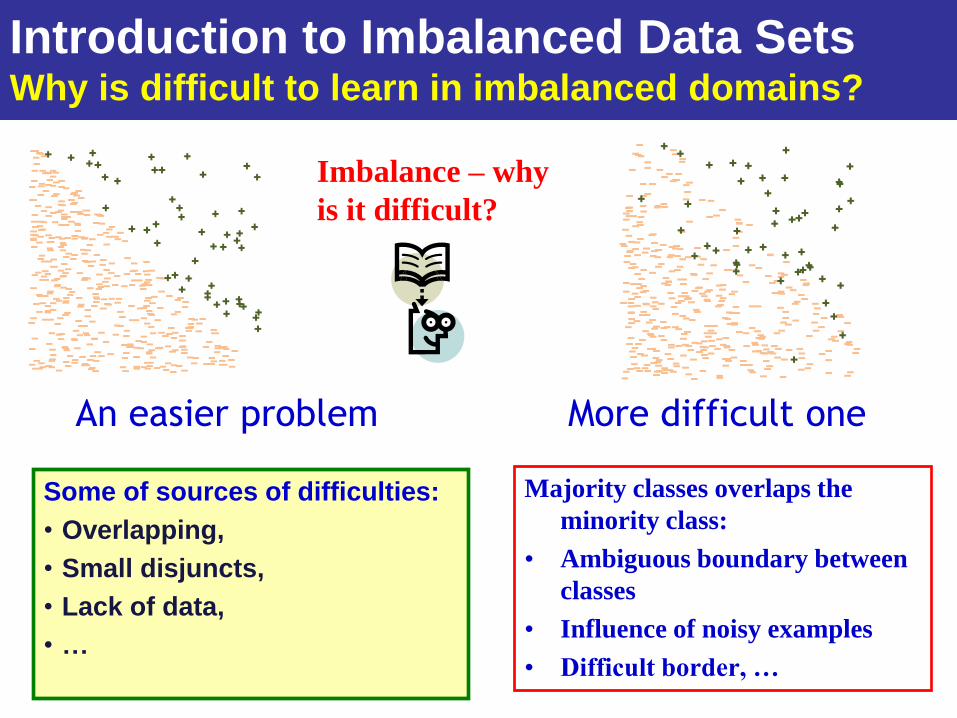
Imbalance – why
is it difficult?
Majority classes overlaps the
minority class:
• Ambiguous boundary between
classes
• Influence of noisy examples
• Difficult border, …
An easier problem More difficult one
Some of sources of difficulties:
• Overlapping,
• Small disjuncts,
• Lack of data,
• …
Introduction to Imbalanced Data Sets Why is difficult to learn in imbalanced domains?

Why is difficult to learn in imbalanced domains?
Intrinsic data characteristics
Overlapping
Small disjuncts/rare data sets
Density: Lack of data
Bordeline and Noise data
Dataset shift
V. López, A. Fernandez, S. García, V. Palade, F. Herrera, An Insight into Classification with Imbalanced
Data: Empirical Results and Current Trends on Using Data Intrinsic Characteristics. Information
Sciences 250 (2013) 113-141.

46
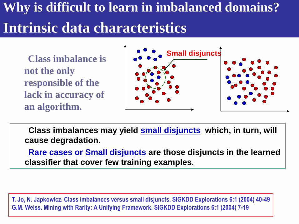
Class imbalance is not the only
responsible of the lack in
accuracy of an algorithm.
V. García, R.A. Mollineda, J.S. Sánchez. On the k-NN performance in a challenging scenario of
imbalance and overlapping. Pattern Anal Applic (2008) 11: 269-280
The class overlapping also
influences the behaviour of the
algorithms, and it is very typical
in these domains.
Why is difficult to learn in imbalanced domains?
Intrinsic data characteristics

• There is an interesting relationship between
imbalance and class overlapping:
V. García, R.A. Mollineda, J.S. Sánchez. On the k-NN performance in a challenging scenario of imbalance and
overlapping. Pattern Anal Applic (2008) 11: 269-280
J. Luengo, A. Fernandez, S. García, F. Herrera, Addressing Data Complexity for Imbalanced Data
Sets: Analysis of SMOTE-based Oversampling and Evolutionary Undersampling. Soft Computing,
15 (10) 1909-1936
Two different levels of class
overlapping: (a) 0% and (b) 60%
47
Why is difficult to learn in imbalanced domains?
Intrinsic data characteristics

• The degree of overlap for
individual feature values is
measured by the metric F1
or maximum Fisher's
discriminant ratio
• We compute f for each
feature and take the
maximum over all
dimensions as metric F1.
F1 = 3.3443
F1 = 0.6094
Why is difficult to learn in imbalanced domains?
Intrinsic data characteristics

• There is an interesting relationship between
imbalance and class overlapping:
49
Why is difficult to learn in imbalanced domains?
Intrinsic data characteristics
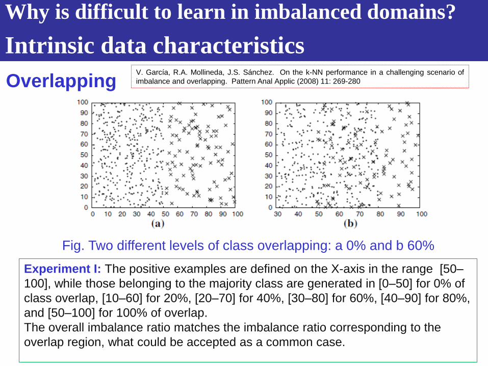
Fig. Two different levels of class overlapping: a 0% and b 60%
Experiment I: The positive examples are defined on the X-axis in the range [50–
100], while those belonging to the majority class are generated in [0–50] for 0% of
class overlap, [10–60] for 20%, [20–70] for 40%, [30–80] for 60%, [40–90] for 80%,
and [50–100] for 100% of overlap.
The overall imbalance ratio matches the imbalance ratio corresponding to the
overlap region, what could be accepted as a common case.
Overlapping
Why is difficult to learn in imbalanced domains?
Intrinsic data characteristics V. García, R.A. Mollineda, J.S. Sánchez. On the k-NN performance in a challenging scenario of
imbalance and overlapping. Pattern Anal Applic (2008) 11: 269-280

Fig. Performance metrics in k-NN rule and other learning algorithms
for experiment I
Overlapping
Why is difficult to learn in imbalanced domains?
Intrinsic data characteristics

Fig. Two different cases in
experiment II: [75-100] and [85-100].
For this latter case, note that in the
overlap region, the majority class is
under-represented in comparison to
the minority class.
Experiment II: The second experiment has been carried out over a collection of five artificial
imbalanced data sets in which the overall minority class becomes the majority in the overlap
region. To this end, the 400 negative examples have been defined on the X-axis to be in the
range [0–100] in all data sets, while the 100 positive cases have been generated in the
ranges [75–100], [80–100], [85–100], [90–100], and [95–100]. The number of elements in the
overlap region varies from no local imbalance in the first case, where both classes have the
same (expected) number of patterns and density, to a critical inverse imbalance in the fifth
case, where the 100 minority examples appears as majority in the overlap region along with
about 20 expected negative examples.
Overlapping
Why is difficult to learn in imbalanced domains?
Intrinsic data characteristics V. García, R.A. Mollineda, J.S. Sánchez. On the k-NN performance in a challenging
scenario of imbalance and overlapping. Pattern Anal Applic (2008) 11: 269-280

Fig. Performance metrics in k-NN rule and other learning algorithms
for experiment II
Overlapping
Why is difficult to learn in imbalanced domains?
Intrinsic data characteristics

54
Conclusions: Results (in this paper) show
that the class more represented in overlap
regions tends to be better classified by
methods based on global learning, while the class less
represented in such regions tends to be better
classified by local methods.
In this sense, as the value of k of the k-NN rule
increases, along with a weakening of its local nature, it
was progressively approaching the behaviour of
global models.
Overlapping
Why is difficult to learn in imbalanced domains?
Intrinsic data characteristics

Why is difficult to learn in imbalanced domains?
Intrinsic data characteristics
Overlapping
Small disjuncts/rare data sets
Density: Lack of data
Bordeline and Noise data
Dataset shift
V. López, A. Fernandez, S. García, V. Palade, F. Herrera, An Insight into Classification with Imbalanced
Data: Empirical Results and Current Trends on Using Data Intrinsic Characteristics. Information
Sciences 250 (2013) 113-141.
Class imbalance is
not the only
responsible of the
lack in accuracy of
an algorithm.
Class imbalances may yield small disjuncts which, in turn, will
cause degradation.
Rare cases or Small disjuncts are those disjuncts in the learned
classifier that cover few training examples.
T. Jo, N. Japkowicz. Class imbalances versus small disjuncts. SIGKDD Explorations 6:1 (2004) 40-49
G.M. Weiss. Mining with Rarity: A Unifying Framework. SIGKDD Explorations 6:1 (2004) 7-19
Small disjuncts
Why is difficult to learn in imbalanced domains?
Intrinsic data characteristics

Learner
Dataset Knowledge Model
Minimize learning error
+
maximize generalization
Rare or exceptional cases correspond to small numbers of training examples in particular areas of the feature space. When learning a concept, the presence of rare cases in the domain is an important consideration. The reason why rare cases are of interest is that they cause small disjuncts to occur, which are known to be more error prone than large disjuncts.
In the real world domains, rare cases are unknown since high dimensional data cannot be visualized to reveal areas of low coverage.
T. Jo, N. Japkowicz. Class imbalances versus small disjuncts. SIGKDD Explorations 6:1 (2004) 40-49
Why is difficult to learn in imbalanced domains?
Intrinsic data characteristics

Rare cases
or Small
disjunct:
Focusing
the problem
Small Disjunct or
Starved niche
Again
more small disjuncts
Overgeneral
Classifier
Rare or excepcional cases
Why is difficult to learn in imbalanced domains?
Intrinsic data characteristics

G.M. Weiss. Mining with Rarity: A Unifying Framework. SIGKDD Explorations 6:1 (2004) 7-19
Class A is the rare (minority
class and B is the common
(majority class).
Subconcepts A2-A5 correspond
to rare cases, whereas A1
corresponds to a fairly common
case, covering a substantial
portion of the instance space.
Subconcept B2 corresponds to a
rare case, demonstrating that
common classes may contain
rare cases.
Rarity: Rare Cases versus
Rare Classes
Rare or excepcional cases
Why is difficult to learn in imbalanced domains?
Intrinsic data characteristics

In the real-word domains, rare cases are not easily identified. An
approximation is to use a clustering algorithm on each class.
Jo and Japkowicz, 2004: Cluster-based oversampling: A method
for inflating small disjuncts.
T. Jo, N. Japkowicz. Class imbalances versus small disjuncts. SIGKDD Explorations 6:1 (2004) 40-49
CBO method:
Cluster-based
resampling identifies
rare cases and re-
samples them
individually, so as to
avoid the creation of
small disjuncts in
the learned
hypothesis.
Small disjuncts/Rare or excepcional cases
Why is difficult to learn in imbalanced domains?
Intrinsic data characteristics

T. Jo, N. Japkowicz. Class imbalances versus small disjuncts. SIGKDD Explorations 6:1 (2004) 40-49
Small disjuncts/Rare or excepcional cases
Why is difficult to learn in imbalanced domains?
Intrinsic data characteristics

Small disjuncts play a role in the performance loss of class imbalanced
domains.
Jo and Japkowicz results show that it is the small disjuncts problem
more than the class imbalance problem that is responsible for the this
decrease in accuracy.
The performance of classifiers, though hindered by class imbalanced, is
repaired as the training set size increases.
T. Jo, N. Japkowicz. Class imbalances versus small disjuncts. SIGKDD Explorations 6:1 (2004) 40-49
An open question: Whether it is more effective to use
solutions that address both the class imbalance and the
small disjunct problem simultaneously than it is to use
solutions that address the class imbalance problem or the
small disjunct problem, alone.
Rare or excepcional cases
Why is difficult to learn in imbalanced domains?
Intrinsic data characteristics

Why is difficult to learn in imbalanced domains?
Intrinsic data characteristics
Overlapping
Small disjuncts/rare data sets
Density: Lack of data
Bordeline and Noise data
Dataset shift
V. López, A. Fernandez, S. García, V. Palade, F. Herrera, An Insight into Classification with Imbalanced
Data: Empirical Results and Current Trends on Using Data Intrinsic Characteristics. Information
Sciences 250 (2013) 113-141.

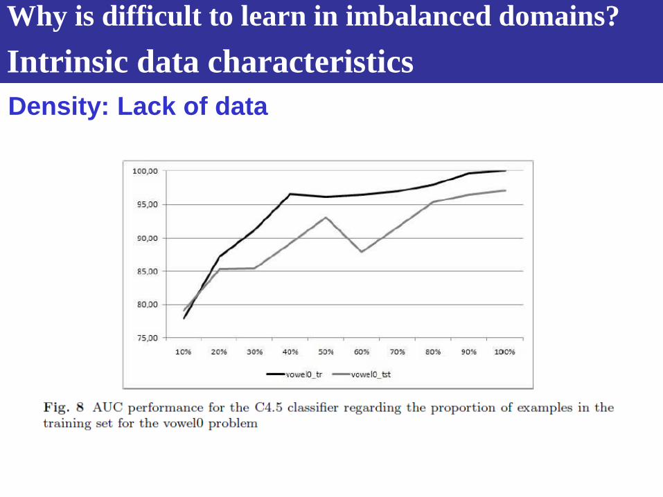
T. Jo, N. Japkowicz. Class imbalances versus small disjuncts. SIGKDD Explorations 6:1 (2004) 40-49
Density: Lack of data
Different
levesl of
imbalance
and
density
Why is difficult to learn in imbalanced domains?
Intrinsic data characteristics

T. Jo, N. Japkowicz. Class imbalances versus small disjuncts. SIGKDD Explorations 6:1 (2004) 40-49
Left-C4.5, right-Backpropagation: These resultas show
that the performance of classifiers, though hindered by
class imbalances, is repaired as the training set size
incresses. This sugests that small disjuncts play a role in
the performance loss of class imbalanced domains.
Density: Lack of data
Why is difficult to learn in imbalanced domains?
Intrinsic data characteristics
Density: Lack of data
Why is difficult to learn in imbalanced domains?
Intrinsic data characteristics

Why is difficult to learn in imbalanced domains?
Intrinsic data characteristics
Overlapping
Small disjuncts/rare data sets
Density: Lack of data
Bordeline and Noise data
Dataset shift
V. López, A. Fernandez, S. García, V. Palade, F. Herrera, An Insight into Classification with Imbalanced
Data: Empirical Results and Current Trends on Using Data Intrinsic Characteristics. Information
Sciences 250 (2013) 113-141.

Four Groups of Negative Examples Noise examples
Borderline examples
Borderline examples are unsafe since a small amount of noise can make them fall on the wrong side of the decision border.
Redundant examples
Safe examples
Kind of examples: The need of resampling or to
manage the overlapping with other strategies
An approach: Detect and remove such
majority noisy and borderline examples in
filtering before inducing the classifier.
Why is difficult to learn in imbalanced domains?
Intrinsic data characteristics

Bordeline and Noise data
Why is difficult to learn in imbalanced domains?
Intrinsic data characteristics

3 kind of artificial problems: Subclus: examples from the minority class are located inside rectangles following related works on
small disjuncts.
Clover: It represents a more difficult, non-linear setting, where the minority class resembles a
flower with elliptic petals.
Paw: The minority class is decomposed into 3 elliptic sub-regions of varying cardinalities, where
two subregions are located close to each other, and the remaining smaller sub-region is separated.
Why is difficult to learn in imbalanced domains?
Intrinsic data characteristics
Bordeline and Noise data
Clover data Paw data Subclus data

Why is difficult to learn in imbalanced domains?
Intrinsic data characteristics
Bordeline and Noise data
Clover data Paw data

Why is difficult to learn in imbalanced domains?
Intrinsic data characteristics
Bordeline and Noise data
Subclus data

Why is difficult to learn in imbalanced domains?
Intrinsic data characteristics
Bordeline and Noise data
Subclus data

SPIDER 2: Spider family (Selective Preprocessing
of Imbalanced Data) rely on the local
characteristics of examples discovered by
analyzing their k-nearest neighbors.
J. Stefanowski, S. Wilk. Selective pre-processing of imbalanced data for improving classification
performance. 10th International Conference in Data Warehousing and Knowledge Discovery
(DaWaK2008). LNCS 5182, Springer 2008, Turin (Italy, 2008) 283-292.
K.Napierala, J. Stefanowski, and S. Wilk. Learning from Imbalanced Data in Presence of Noisy and
Borderline Examples. 7th International Conference on Rough Sets and Current Trends in Computing , 7th
International Conference on Rough Sets and Current Trends in Computing, RSCTC 2010, LNAI 6086, pp. 158–
167, 2010.
Why is difficult to learn in imbalanced domains?
Intrinsic data characteristics
Bordeline and Noise data

Why is difficult to learn in imbalanced domains?
Intrinsic data characteristics
Bordeline and Noise data
Noise data

Why is difficult to learn in imbalanced domains?
Intrinsic data characteristics
Bordeline and Noise data
Small disjunct and Noise data
Bordeline and Noise data
Bordeline and Noise data

• SPIDER 2: allows to get good results in comparison with
classical ones.
• It has interest to analyze the use of noise filtering algorithms for
these problems: IPF filtering algorithm shows good results.
José A. Sáez, J. Luengo, Jerzy Stefanowski, F. Herrera, SMOTE–IPF: Addressing the
noisy and borderline examples problem in imbalanced classification by a re-
sampling method with filtering. Information Sciences 291 (2015) 184-203, doi:
10.1016/j.ins.2014.08.051.
• Specific methods for managing the noise and bordeline
problems are necessary.
Why is difficult to learn in imbalanced domains?
Intrinsic data characteristics
Bordeline and Noise data
Why is difficult to learn in imbalanced domains?
Intrinsic data characteristics
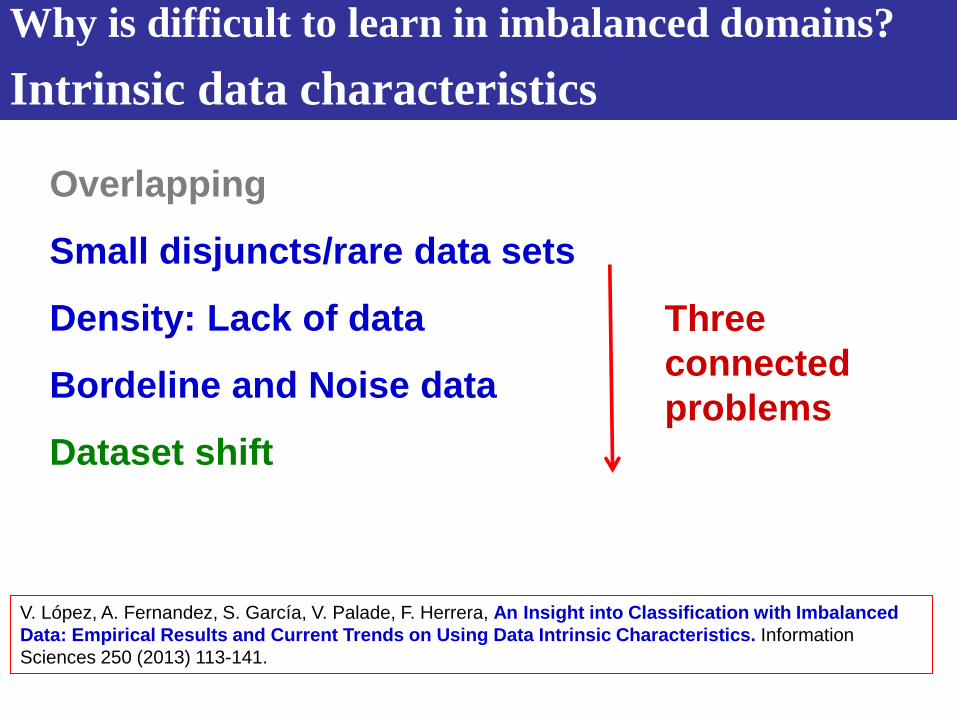
Overlapping
Small disjuncts/rare data sets
Density: Lack of data
Bordeline and Noise data
Dataset shift
Three
connected
problems
V. López, A. Fernandez, S. García, V. Palade, F. Herrera, An Insight into Classification with Imbalanced
Data: Empirical Results and Current Trends on Using Data Intrinsic Characteristics. Information
Sciences 250 (2013) 113-141.

Rare cases may be due to a lack of data. Relative
lack of data, relative rarity.
G.M. Weiss. Mining with Rarity: A Unifying Framework. SIGKDD Explorations 6:1 (2004) 7-19
Small disjuncts and density
Why is difficult to learn in imbalanced domains?
Intrinsic data characteristics

Noise data will affect the way any data mining
system behaves. Noise has a greater impact on
rare cases than on common cases.
G.M. Weiss. Mining with Rarity: A Unifying Framework. SIGKDD Explorations 6:1 (2004) 7-19
Why is difficult to learn in imbalanced domains?
Intrinsic data characteristics
Small disjuncts and Noise data
Why is difficult to learn in imbalanced domains?
Intrinsic data characteristics
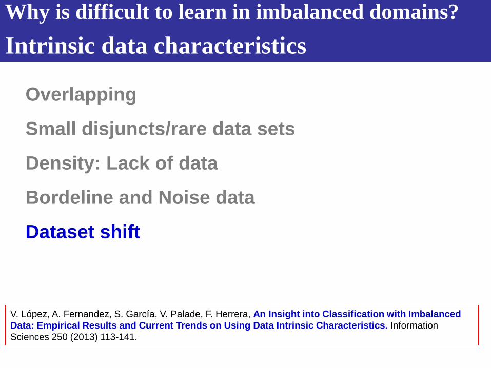
Overlapping
Small disjuncts/rare data sets
Density: Lack of data
Bordeline and Noise data
Dataset shift
V. López, A. Fernandez, S. García, V. Palade, F. Herrera, An Insight into Classification with Imbalanced
Data: Empirical Results and Current Trends on Using Data Intrinsic Characteristics. Information
Sciences 250 (2013) 113-141.

Why is difficult to learn in imbalanced domains?
Intrinsic data characteristics
Dataset shift

Why is difficult to learn in imbalanced domains?
Intrinsic data characteristics
Dataset shift
• The classifier has an overfitting problem.
• Is there a change in data distribution between
training and test sets (Data fracture)?.

The Problem of Dataset Shift
• The classifier has an overfitting problem. – Change the parameters of the algorithm.
– Use a more general learning method.
• There is a change in data distribution
between training and test sets (Dataset shift). – Train a new classifier for the test set.
– Adapt the classifier.
– Modify the data in the test set …

The Problem of Dataset Shift
The problem of data-set shift is defined as the case where training
and test data follow different distributions.
J. G. Moreno-Torres, T. R. Raeder, R. Aláiz-Rodríguez, N. V. Chawla, F. Herrera, A unifying view on
dataset shift in classification. Pattern Recognition 45:1 (2012) 521-530,
doi:10.1016/j.patcog.2011.06.019.

This is a common problem that can affect all kind of classification
problems, and it often appears due to sample selection bias issues.
However, the data-set shift issue is specially relevant when dealing
with imbalanced classification, because in highly imbalanced domains,
the minority class is particularly sensitive to singular classification errors,
due to the typically low number of examples it presents.
In the most extreme cases, a single misclassified example of the minority
class can create a significant drop in performance.
Why is difficult to learn in imbalanced domains?
Intrinsic data characteristics
Dataset shift

Why is difficult to learn in imbalanced domains?
Intrinsic data characteristics
Dataset shift
Since dataset shift is a highly relevant issue in imbalanced classification,
it is easy to see why it would be an interesting perspective to focus on future
research regarding the topic.

Causes of Dataset Shift
We comment on some of the most common
causes of Dataset Shift:
Sample selection bias and non-stationary
environments.
These concepts have created confusion at times,
so it is important to remark that these terms are
factors that can lead to the appearance of
some of the shifts explained, but they do not
constitute Dataset Shift themselves.

Causes of Dataset Shift
Sample selection
bias:

• Training and test following the same data distribution
Original Data
Training Data Test Data
Causes of Dataset Shift

• DATASET SHIT: Training and test following different
data distribution
Original Data
Training Data Test Data
Causes of Dataset Shift

Sample bias selection: Influence of partitioning on classifiers' performance
Classifier performance results
over two separate iterations of
random 10-fold cross-
validation.
A consistent random number
seed was used across al
datasets within an iteration.
T. Raeder, T. R. Hoens, and N. V. Chawla,
“Consequences of variability in classifier
performance estimates,” Proceedings of
the 2010 IEEE International Conference
on Data Mining, 2010, pp. 421–430.
Causes of Dataset Shift
Wilcoxon test: Clear differences for both algorithms

source domain target domain Causes of Dataset Shift
Causes of Dataset Shift Challenges in correcting the dataset shift generated by the sample selection bias

source domain target domain
Causes of Dataset Shift Challenges in correcting the dataset shift generated by the sample selection bias

Where Does the Difference Come from?
p(x, y)
p(x)p(y | x)
ptra(y | x) ≠ ptst(y | x)
ptra(x) ≠ ptst(x)
labeling difference instance difference
labeling adaptation instance adaptation ?
Causes of Dataset Shift Challenges in correcting the dataset shift generated by the sample selection bias

Why is difficult to learn in imbalanced domains?
Intrinsic data characteristics
Dataset shift
Moreno-Torres, J. G., & Herrera, F. (2010). A preliminary study on overlapping and data fracture in imbalanced domains by means of
genetic programming-based feature extraction. In Proceedings of the 10th International Conference on Intelligent Systems Design
and Applications (ISDA 2010) (pp. 501–506).
Why is difficult to learn in imbalanced domains?
Intrinsic data characteristics
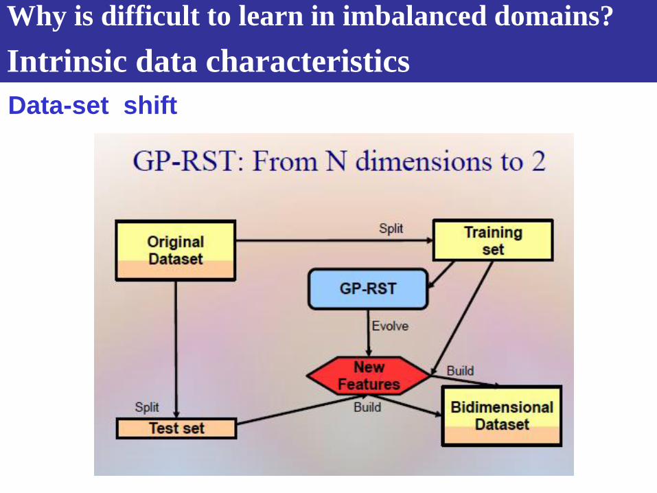
Data-set shift

A Genetic-Programming based Feature Selection
and RST for Visualization of Fracture between Data
The quality of approximation
is the proportion of the elements
of a rough set that belong to its
lower approximation.

Good behaviour. pageblocks 13v4, 1st partition.
A Genetic-Programming based Feature Selection
and RST for Visualization of Fracture between Data
(a) Training set (1.0000) (b) Test set (1.0000)

Dataset shift. ecoli 4, 1st partition.
A Genetic-Programming based Feature Selection
and RST for Visualization of Fracture between Data
(a) Training set (0.9663) (b) Test set (0.8660)

Overlap and dataset shift. glass 016v2, 4th partition.
(a) Training set (0.3779) (b) Test set (0.0000)
A Genetic-Programming based Feature Selection
and RST for Visualization of Fracture between Data

Overlap and dataset shift. glass 2, 2nd partition
(a) Training set (0.6794) (b) Test set (0.0000)
A Genetic-Programming based Feature Selection
and RST for Visualization of Fracture between Data

There are two different potential approaches in the study of the
effect and solution of data-set shift in imbalanced domains.
The first one focuses on intrinsic data-set shift, that is, the data of
interest includes some degree of shift that is producing a relevant drop in
performance. In this case, we need to:
Develop techniques to discover and measure the presence of
data-set shift adapting them to minority classes.
Design algorithms that are capable of working under data-set shift
conditions. These could be either preprocessing techniques or
algorithms that are designed to have the capability to adapt and deal
with dataset shift without the need for a preprocessing step.
Why is difficult to learn in imbalanced domains?
Intrinsic data characteristics
Dataset shift

The second branch in terms of data-set shift in imbalanced
classification is related to induced data-set shift.
Most current state of the art research is validated through stratified cross-
validation techniques, which are another potential source of shift in the
machine learning process.
A more suitable validation technique needs to be developed in
order to avoid introducing data-set shift issues artificially.
Why is difficult to learn in imbalanced domains?
Intrinsic data characteristics
Dataset shift

Why is difficult to learn in imbalanced domains?
Intrinsic data characteristics
Dataset shift
Imbalanced classification problems are difficult
when overlap and/or data fracture are present.
Single outliers can have a great influence on
classifier performance.
This is a novel problem in imbalanced
classification that need a lot of studies.

Overlapping
Rare sets/ Small disjuncts: The class imbalance problem
may not be a problem in itself. Rather, the small disjunct
problem it causes is responsible for the decay.
The overall size of the training set
large training sets yield low sensitivity to class
imbalances
Noise and border data provokes additional problems.
An increase in the degree of class imbalance. The data
partition provokes data fracture: Dataset shift.
What domain characteristics aggravate the problem?
Why is difficult to learn in imbalanced domains?
Intrinsic data characteristics

I. Introduction to imbalanced data sets
II. Why is difficult to learn in imbalanced domains?
Intrinsic data characteristics
III. Class imbalance: Data sets, implementations, …
IV. Class imbalance: Trends and final comments
Contents

KEEL Data Mining Tool:
It includes algorithms
and data set partitions
http://www.keel.es
Class Imbalance: Data sets,
implementations, …

It contains a big collection of classical knowledge
extraction algorithms, preprocessing techniques.
It includes a large list of algorithms for imbalanced
data.
KEEL is an open source (GPLv3) Java
software tool to assess evolutionary
algorithms for Data Mining problems
including regression, classification,
clustering, pattern mining and so on.
Class Imbalance: Data sets,
implementations, …

Class Imbalance: Data sets,
implementations, …
We include 111 data sets:
66 for 2 classes,
15 for multiple classes and
30 for noise and bordeline.
We also include the preprocessed data sets.

I. Introduction to imbalanced data sets
II. Why is difficult to learn in imbalanced domains?
Intrinsic data characteristics
III. Class imbalance: Data sets, implementations, …
IV. Class imbalance: Trends and final comments
Contents

Y.
Su
n,
A.
K.
C.
Wo
ng
a
nd
M
. S
. K
am
el.
Cla
ssif
ica
tio
n o
f im
ba
lan
ced
d
ata
: A
re
vie
w.
Inte
rn
ati
on
al
Jo
urn
al
of
Pa
tte
rn
Re
co
gn
itio
n
23:4
(2009
) 687-7
19.
Class Imbalance: Trends and final comments Data level vs algorithm Level

Class Imbalance vs. Asymmetric Misclassification costs
Class Imbalance: Trends and final comments New
studies, trends and challenges
Improvements on resampling – specialized resampling
New approches for creating artificial instances
How to choose the amount to sample?
New hybrid approaches oversampling vs undersampling
Cooperation between resampling/cost sensitive/boosting
Cooperation between feature selection and resampling
Scalability: high number of features and sparse data
Intrinsic data characteristics. To analyze the challenges on
the class distribution.

Class Imbalance vs. Asymmetric Misclassification costs
Class Imbalance: Trends and final comments New
studies, trends and challenges
In short, it is necessary to do work for:
Establishing some fundamental results regarding:
a) the nature of the problem,
b) the behaviour of different types of classifiers, and
c) the relative performance of various previously
proposed schemes for dealing with the problem.
Designing new methods addressing the problem.
Tackling data preprocessing and changing rule
classification strategy.

Class Imbalance vs. Asymmetric Misclassification costs
Class Imbalance: Trends and final
comments Final comments
Class imbalance is a challenging and critical
problem in the knowledge discovery field, the
classification with imbalanced data sets.
Due to the intriguing topics and tremendous
potential applications, the classification of
imbalanced data will continue to receive
more and more attention along next years.
Class of interest is often much smaller or
rarer (minority class).

1. Clasificación no balanceada
2. Multiclasificadores: Bagging y Boosting
3. Multiples clases: Descomposición binaria
4. Redes Neuronales y Maquinas de soporte Vectorial
Sistemas Inteligentes para la Gestión de la Empresa
TEMA 3. Análisis Predictivo para la
Empresa
(Modelos predictivos avanzados de clasificación)

117
Algunos ejemplos de clasificadores sencillos Clasificador Del Vecino Más Cercano (k-NN): Basado en
distancias (muy diferente a los basados en particiones)
2. Multiclasificadores

118
Algunos ejemplos de clasificadores sencillos Clasificador basado en particiones y reglas – Arboles de
decisión
2. Multiclasificadores

119
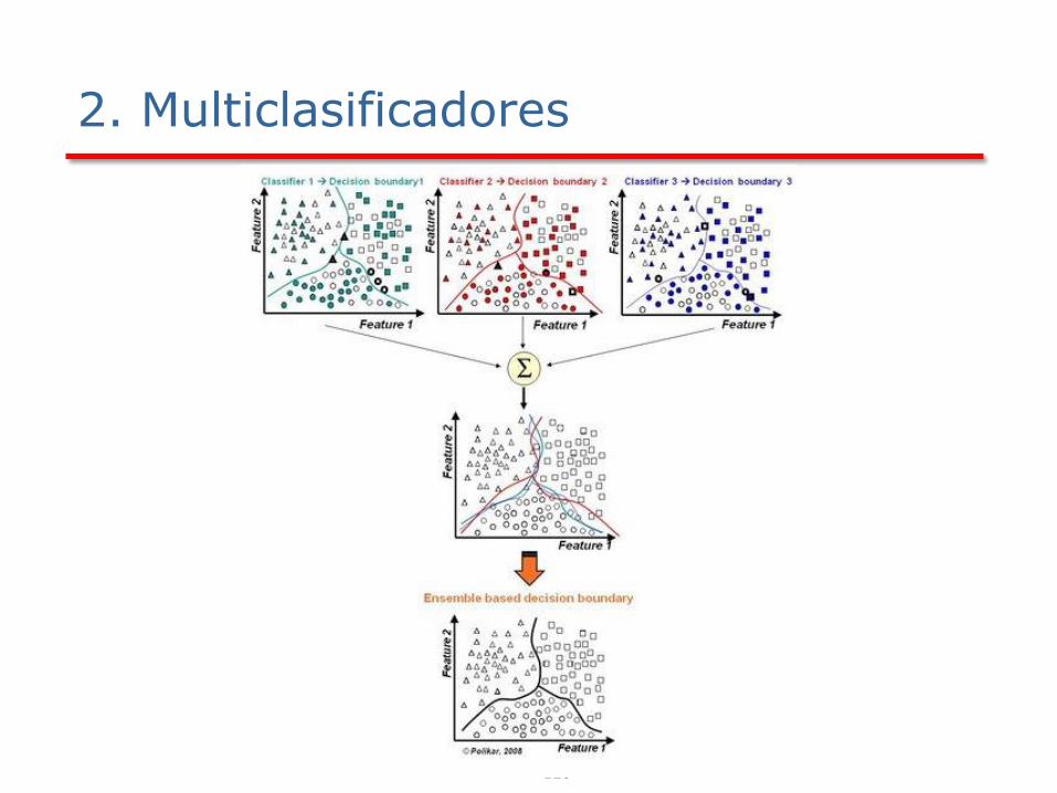
2. Multiclasificadores
La idea es inducir n clasificadores en lugar de uno solo
Para clasificar se utilizará una combinación de la salida que proporciona cada clasificador
Los clasificadores pueden estar basados en distintas técnicas (p.e. árboles, reglas, instancias,…)
Se puede aplicar sobre el mismo clasificador o con diferentes.
Modelos específicos: • Bagging: cada clasificador se induce independientemente
incluyendo una fase de diversificación sobre los datos
• Boosting: cada clasificador tiene en cuenta los fallos del anterior
120
2. Multiclasificadores

121
2. Multiclasificadores: Bagging
Bagging definido a partir de “bootstrap aggregating”.
Un método para combinar múltiples predictores/clasificadores.
Bagging funciona bien para los algoritmos de aprendizaje "inestables“, aquellos para los que un pequeño cambio en el conjunto de entrenamiento puede provocar grandes cambios en la predicción (redes neuronales, árboles de decisión, redes neuronales, …) (No es el caso de k-NN que es un algoritmo estable)

122
2. Multiclasificadores: Bagging

123
2. Multiclasificadores: Bagging
Fase 1: Generación de modelos
1. Sea n el número de ejemplos en la BD y m el número de los modelos a utilizar
2. Para i=1,…,m hacer
• Muestrear con reemplazo n ejemplos de la BD (Boosting)
• Aprender un modelo con ese conjunto de entrenamiento
• Almacenarlo en modelos[i]
• Fase 2: Clasificación
1. Para i=1,…,m hacer
• Predecir la clase
utilizando modelos[i]
2. Devolver la clase predicha
con mayor frecuencia

124
2. Multiclasificadores: Bagging

125
2. Multiclasificadores: Bagging
Random Forest (Leo Breiman, Adele Cutler): Boostraping (muestreo con
reemplazamiento, 66%), Selección aleatoria de un conjunto muy pequeño de
variables (m<<M) (ej. log M + 1) para elegir entre ellas el atributo que
construye el árbol (medida de Gini),
sin poda (combinación de
clasificadores débiles)
Breiman, Leo (2001). «Random Forests».
Machine Learning 45 (1): pp. 5–32.
doi:10.1023/A:1010933404324

126
3. Multiclasificadores: Boosting
Muestreo ponderado (ejemplos):
• En lugar de hacer un muestreo aleatorio de los datos de entrenamiento, se ponderan las muestras para concentrar el aprendizaje en los ejemplos más difíciles.
• Intuitivamente, los ejemplos más cercanos a la frontera de decisión son más difíciles de clasificar, y recibirán pesos más altos.
Votos ponderados (clasificadores):
• En lugar de combinar los clasificadores con el mismo peso en el voto, se usa un voto ponderado.
• Esta es la regla de combinación para el conjunto de clasificadores débiles.
• En conjunción con la estrategia de muestreo anterior, esto produce un clasificador más fuerte.

127
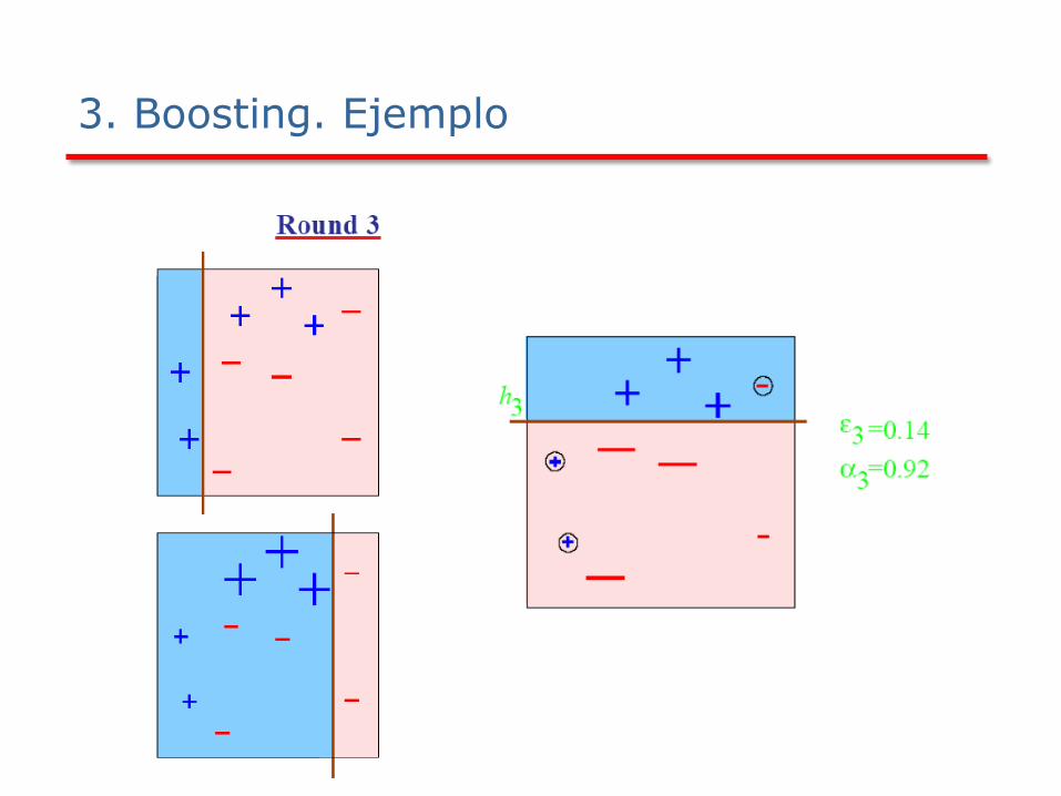
3. Multiclasificadores: Boosting
Idea

128
3. Multiclasificadores: Boosting
Los modelos no se construyen independientemente, sino que el modelo i-ésimo está influenciado por los anteriores
La idea es prestar más atención a los ejemplos mal clasificados por los modelos anteriores
Fase 1: Generación de modelos 1. Asignar a cada ejemplo el mismo peso (1/n)
2. Para i=1,…,m hacer • Aprender un modelo a partir de la BD con pesos
• Almacenarlo en modelos[i]
• Calcular el error εi sobre el conjunto de ejemplos
• Si εi=0 o εi>=0.5 terminar
• Para cada ejemplo bien clasificado multiplicar su peso por εi/(1-εi)
• Normalizar los pesos de todos los ejemplos
• Fase 2: Clasificación
1. Asignar peso cero a todas las categorías de la variable clase
2. Para i=1,…,m hacer • Sumar –log(εi/(1-εi)) a la categoría predicha por modelos[i]
3. Devolver la categoría con
mayor peso

129
3. Multiclasificadores: Boosting
AdaBoost, abreviatura de "Adaptive Boosting", es un algoritmo de aprendizaje meta-algoritmo formulado por Yoav Freund y Robert Schapire que ganó el prestigioso "Premio Gödel" en 2003 por su trabajo. Se puede utilizar en conjunción con muchos otros tipos de algoritmos de aprendizaje para mejorar su rendimiento.
La salida de los otros
algoritmos de aprendizaje
(“algoritmos débiles”)
se combina en una suma
ponderada que representa
la salida final del
clasificador impulsado.

130
3. Multiclasificadores: Boosting

131
3. Boosting. Ejemplo

132
3. Boosting. Ejemplo
133
3. Boosting. Ejemplo

134
3. Boosting. Ejemplo

Bagging and Boosting
Resumen: Idea General
Training data
Altered Training data
Altered Training data
……..
Aggregation ….
Classifier C
Classification method (CM)
CM
Classifier C1
CM
Classifier C2
Classifier C*
Bagging and Boosting

Bagging and Boosting
Bagging and Boosting
Bagging=
Manipulation
with data set
Boosting =
Manipulation with
model
Resumen:

Bagging and Boosting, Poda de los clasificadores
Bagging and Boosting
La idea general consiste en crear un pool de clasificadores más grande de lo
habitual y luego reducirlo para quedarnos con los que forman el ensemble más
preciso. Esta forma de selección de clasificadores se denomina "ensemble pruning".
Los modelos basados en ordenamiento generalmente parten de añadir 1 clasificador
al modelo final. Posteriormente, en cada iteración añaden un nuevo clasificador del
pool de los no seleccionados en base a una medida establecida. Y generalmente lo
hacen hasta llegar a un número de clasificadores establecido. Según este artículo,
en Bagging, teniendo un pool de 100 clasificadores, es suficiente con usar 21.
Boosting-based (BB): Hace un boosting a posteriori (muy interesante!). Coge el
clasificador que minimiza más el coste respecto a boosting, pero no los entrena
respecto a esos costes porque los clasificadores ya están en el pool.

1. Clasificación no balanceada
2. Multiclasificadores: Bagging y Boosting
3. Multiples clases: Descomposición binaria
4. Redes Neuronales y Maquinas de soporte Vectorial
Sistemas Inteligentes para la Gestión de la Empresa
TEMA 3. Análisis Predictivo para la
Empresa
(Modelos predictivos avanzados de clasificación)

3. Descomposición de problemas multiclase. Binarización
Descomposición de un problema con múltiples clases
• Estrategia Divide y Vencerás
• Multi-clase Es más fácil resolver problemas
binarios
Para cada problema binario • 1 clasificador binario = clasificador base
Problem • ¿Cómo hacer la descomposición?
• ¿Cómo agregar las salidas?
Aggregation or
Combination
Classifier_1
Classifier_i
Classifier_n
Final Output

3. Descomposición de problemas multiclase. Binarización
Una aplicación real en KAGGLE de Problema Multiclase

3. Descomposición de problemas multiclase. Binarización
Una aplicación real en KAGGLE de Problema Multiclase
For this competition, we have
provided a dataset with 93
features for more than 200,000
products. The objective is to
build a predictive model
which is able to distinguish
between our main product
categories. The winning
models will be open sourced.

3. Descomposición de problemas multiclase. Binarización
Una aplicación real en KAGGLE de Problema Multiclase

3. Descomposición de problemas multiclase. Binarización
Una aplicación real en KAGGLE de Problema Multiclase

3. Descomposición de problemas multiclase. Binarización
Una aplicación real en KAGGLE de Problema Multiclase

3. Descomposición de problemas multiclase. Binarización
Una aplicación real en KAGGLE de Problema Multiclase

Estrategias de descomposición: “One-vs-One” (OVO)
• 1 problema binario para cada par de clases
Nombres en la literatura: Pairwise Learning, Round Robin, All-vs-All…
Total = m(m-1) / 2 classificadores
Decomposition Aggregation
3. Descomposición de problemas multiclase. Binarización

3. Descomposición de problemas multiclase. Binarización

3. Descomposición de problemas multiclase. Binarización

3. Descomposición de problemas multiclase. Binarización

3. Descomposición de problemas multiclase. Binarización

3. Descomposición de problemas multiclase. Binarización
Fase de agregación • Se proponen diferentes vías para combinar los
clasificadores base y obtener la salida final (clase).
Se comienza por una matriz de ratios de clasif.
• rij = confianza del clasificador en favor de la clase i
• rji = confianza del clasificador en favor de la clase j Usualmente: rji = 1 – rij
• Se pueden plantear diferentes formas de combinar estos ratios.
Pairwise Learning: Combinación de las salidas

Otra estrategia de descomposición: One vs All (OVA)
3. Descomposición de problemas multiclase. Binarización

Otra estrategia de descomposición: One vs All (OVA)
3. Descomposición de problemas multiclase. Binarización
Decomposition
Aggregation

3. Descomposición de problemas multiclase. Binarización
Other approaches
• ECOC (Error Correcting Output Code) [Allwein00]
Unify (generalize) OVO and OVA approach
Code-Matrix representing the decomposition • The outputs forms a code-word
• An ECOC is used to decode the code-word
o The class is given by the decodification
Class Classifier
C1 C2 C3 C4 C5 C5 C7 C8 C9
Class1 1 1 1 0 0 0 1 1 1
Class2 0 0 -1 1 1 0 1 -1 -1
Class3 -1 0 0 -1 0 1 -1 1 -1
Class4 0 -1 0 0 -1 -1 -1 -1 1
[Allwein00] E. L. Allwein, R. E. Schapire, Y. Singer, Reducing multiclass to binary: A unifying
approach for margin classifiers, Journal of Machine Learning Research 1 (2000) 113–141.

Ventajas:
• Clasificadores más pequeños (menor número de
instancias)
• Fronteras de decisión más simples
Un algoritmo que está en el “estado del arte” en
comportamiento y utiliza la estrategia OVO para múltiples
clases: SVM (Support Vector Machine).
3. Descomposición de problemas multiclase. Binarización
Estudios sobre la descomposición binaria:
M. Galar, A. Fernandez, E. Barrenechea, H. Bustince, F. Herrera, An Overview of Ensemble Methods for
Binary Classifiers in Multi-class Problems: Experimental Study on One-vs-One and One-vs-All Schemes.
Pattern Recognition 44:8 (2011) 1761-1776, doi: 10.1016/j.patcog.2011.01.017
Anderson Rocha and Siome Goldenstein. Multiclass from Binary: Expanding One-vs-All, One-vs-One and
ECOC-based Approaches. IEEE Transactions on Neural Networks and Learning Systems Vol. 25, Num.
2, pgs. 289–302, 2014 doi:10.1109/TNNLS.2013.2274735

1. Clasificación no balanceada
2. Multiclasificadores: Bagging y Boosting
3. Multiples clases: Descomposición binaria
4. Redes Neuronales y Maquinas de soporte Vectorial
Sistemas Inteligentes para la Gestión de la Empresa
TEMA 3. Análisis Predictivo para la
Empresa
(Modelos predictivos avanzados de clasificación)

157
4. Clasificadores basados en redes neuronales Redes neuronales Surgieron como un intento de emulación de los sistemas
nerviosos biológicos Actualmente: computación modular distribuida mediante la
interconexión de una serie de procesadores (neuronas) elementales

158
4. Clasificadores basados en redes neuronales Redes neuronales Ventajas:
• Habitualmente gran tasa de acierto en la predicción • Son más robustas que los árboles de decisión por los pesos • Robustez ante la presencia de errores (ruido, outliers,…) • Gran capacidad de salida: nominal, numérica, vectores,… • Eficiencia (rapidez) en la evaluación de nuevos casos • Mejoran su rendimiento mediante aprendizaje y éste puede continuar después de
que se haya aplicado al conjunto de entrenamiento
Desventajas: • Necesitan mucho tiempo para el entrenamiento • Entrenamiento: gran parte es ensayo y error • Poca (o ninguna) interpretabilidad del modelo (caja negra) • Difícil de incorporar conocimiento del dominio • Los atributos de entrada deben ser numéricos • Generar reglas a partir de redes neuronales no es inmediato • Pueden tener problemas de sobreaprendizaje
¿Cuándo utilizarlas?
• Cuando la entrada tiene una dimensión alta • La salida es un valor discreto o real o un vector de valores • Posibilidad de datos con ruido • La forma de la función objetivo es desconocida • La interpretabilidad de los resultados no es importante

159
4. Clasificadores basados en redes neuronales
- Las señales que llegan a las dendritas se representan como x1, x2, ..., xn
- Las conexiones sinápticas se representan por unos pesos wj1, wj2, wjn que ponderan
(multiplican) a las entradas. Si el peso entre las neuronas j e i es:
a) positivo, representa una sinapsis excitadora
b) negativo, representa una sinapsis inhibidora
c) cero, no hay conexión
La acción integradora del cuerpo celular (o actividad interna de cada célula) se presenta por
La salida de la neurona se representa por yj. Se obtiene mediante una función que, en general, se denomina función de salida, de transferencia o de activación. Esta función depende de Netj y de un parámetro j que representa el umbral de activación de la neurona
Netj
x1
x2
xn
wj1
wj2
wjn
yj
n
i
ijinjnjjj xwxwxwxwNet1
2211
ijijjj xwfNetfy )(

160
4. Clasificadores basados en redes neuronales
f(.)
x1
x2 y
w1
wn
w2
xn
función de
activación
Sumador
pesos sinápticos
salida
Entradas -1
s
Con función de activación o transferencia tipo salto o “escalón”
El umbral se puede interpretar como un peso sináptico que se aplica a una entrada que vale siempre -1

161
4. Clasificadores basados en redes neuronales
Función de escalón. Representa una neurona con sólo dos estados de activación: activada (1) y inhibida (0 ó -1)
Función lineal:
Función lineal a tramos:
Función sigmoidal:
Función base radial:
jj
jj
jjj Netsi
NetsiNetHy
,1
,1)(
jjj Nety
aNetsi
aNetsiNet
aNetsi
y
jj
jjjj
jj
j
,1
,
,1
11
2
1
1)()(
jjjj NetjNetje
ye
y
2
jjNet
j ey
162
4. Clasificadores basados en redes neuronales
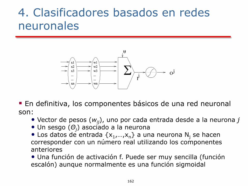
En definitiva, los componentes básicos de una red neuronal son:
• Vector de pesos (wij), uno por cada entrada desde a la neurona j • Un sesgo (Θj) asociado a la neurona • Los datos de entrada {x1,…,xn} a una neurona Nj se hacen corresponder con un número real utilizando los componentes anteriores • Una función de activación f. Puede ser muy sencilla (función escalón) aunque normalmente es una función sigmoidal

163
4. Clasificadores basados en redes neuronales
Resolver un problema de clasificación con una red neuronal implica • Determinar (habitualmente con conocimiento experto)
el número de nodos de salida, el número de nodos de entrada (y los atributos
correspondientes, el número de capas ocultas
• Determinar pesos y funciones a utilizar • Para cada tupla en el conjunto de entrenamiento
propagarlo en la red y evaluar la predicción de salida con el resultado actual. Si la predicción es precisa, ajustar los pesos para asegurar que
esa predicción tendrá un peso de salida más alto la siguiente vez
Si la predicción no es precisa, ajustar los pesos para que la siguiente ocasión se obtenga un valor menor para dicha clase
• Para cada tupla en el conjunto de test propagarla por la red para realizar la clasificación

164
4. Clasificadores basados en redes neuronales El aprendizaje de la estructura de una red neuronal requiere
experiencia, aunque existen algunas guías
Entradas: Por cada variable numérica o binaria/booleana se pone una neurona de entrada. Por cada variable nominal (con más de dos estados) se pone una neurona de entrada por cada estado posible.
Salidas: Si es para predicción se pone una única neurona de salida por cada valor de la variable clase
Capas ocultas. Hay que indicar cuántas capas y cuantas neuronas hay que poner en cada capa. En Weka, • 0: No se pone capa oculta (sólo particiones lineales¡) • Números enteros separados por comas: cada número representa la cantidad
de neuronas de esa capa. P.e. 4,3,5: representa una red con tres capas ocultas de 4, 3 y 5 neuronas respectivamente
• Algunos comodines: i/o: neuronas en la entrada/salida t: i+o a: t/2 (es el valor por defecto)
Cuando la red neuronal está entrenada, para clasificar una instancia,
se introducen los valores de la misma que corresponden a las variables de los nodos de entrada. • La salida de cada nodo de salida indica la probabilidad de que la instancia
pertenezca a esa clase • La instancia se asigna a la clase con mayor probabilidad

165
4. Clasificadores basados en redes neuronales
Clasificadores basados en Redes neruronales

166
4. Clasificadores basados en redes neuronales
Todas las variables numéricas se normalizan [-1,1]
Algoritmo de Backprogation o retropropagación: • Basado en la técnica del gradiente descendiente • No permite conexiones hacia atrás (retroalimentación) en
la red
Esquema del algoritmo de retropropagación
1. Inicializar los pesos y sesgos aleatoriamente 2. Para r=1 hasta número de epoch hacer
a) Para cada ejemplo e de la BD hacer b) Lanzar un proceso forward de propagación en la red neuronal
para obtener la salida asociada a e usando las expresiones vistas anteriormente
c) Almacenar el valor Oj producido en cada neurona Nj
d) Lanzar un proceso backward para recalcular los pesos y los sesgos asociados a cada neurona
1 epoch = procesamiento de todos los ejemplos de la BD

167
4. Clasificadores basados en redes neuronales
Fase de retropagación:
• Para cada neurona de salida Ns hacer BP(Ns)
• BP(Nj):
1. Si Nj es una neurona de entrada, finalizar
2. Si Nj es una neurona de salida
entonces Errj = Oj·(1-Oj)·(Tj-Oj)
si no Errj = Oj(1-Oj) Σk de salida Errk · wjk
con Tj el valor predicho en la neurona Nj
3. Actualizar los pesos wij = wij+α·Errj·Oi
4. Actualizar los sesgos: Θj = Θj + α·Errj
5. Para cada neurona Ni tal que Ni Nj hacer BP(Ni)

168
4. Clasificadores basados en redes neuronales
En definitiva,
Inicializar todos los pesos a números aleatorios pequeños
Hasta que se verifique la condición de parada hacer
• Para cada ejemplo de entrenamiento hacer
Introducir el ejemplo en la red y propagarla para obtener la salida (Ok)
Para cada unidad de salida k
• Error k Ok(1-Ok)(tk-Ok)
Para cada unidad oculta
• Error k Ok(1-Ok)∑j salida wk,j errorj
Modificar cada peso de la red
• wi,j wi,j + Δwij
• Δwi,j = η Errorj xi,j

169
4. Clasificadores basados en redes neuronales
Existen muchos otros modelos de redes neuronales (recurrentes, memorias asociativas, redes neuronales de base radial, redes ART, …)
El término de Deep Learning (procesamiento masivo de datos que utiliza redes neuronales) ha centrado la atención en modelos escalables de redes neuronales
Google cuenta, desde hace tres años con el departamento conocido como ‘ Google Brain’ (dirigido por Andrew Ng, Univ. Stanford, responsable de un curso de coursera de machine learning) dedicado a esta técnica entre otras. En 2013, Google adquirió la compañía DNNresearch Inc de uno de los padres del Deep Learning (Geoffrey Hinton). En enero de 2014 se hizo con el control de la ‘startup’ Deepmind Technologies una pequeña empresa londinense en la trabajaban que algunos de los mayores expertos en ‘deep learning’.

170
4. Clasificadores basados en máquinas de soporte vectorial (SVM)
“Una SVM(support vector machine) es un modelo de aprendizaje que se fundamenta en la Teoría de Aprendizaje Estadístico. La idea básica es encontrar un hiperplano canónico que maximice el margen del conjunto de datos de entrenamiento, esto nos garantiza una buena capacidad de generalización.”
Representación dual de un problema
+ Funciones Kernel
+ Teoría de Aprendizaje Estadística
+ Teoría Optimización Lagrange
=

171
4. Clasificadores basados en máquinas de soporte vectorial (SVM)
Una SVM es un máquina de aprendizaje lineal (requiere que los datos sean linealmente separables).
Estos métodos explotan la información que proporciona el producto interno (escalar) entre los datos disponibles.
La idea básica es:

172
4. Clasificadores basados en máquinas de soporte vectorial (SVM)
Problemas de esta aproximación:
¿Cómo encontrar la función ?
El espacio de características inducido H es de alta dimensión.
Problemas de cómputo y memoria.

173
4. Clasificadores basados en máquinas de soporte vectorial (SVM)
Solución:
Uso de funciones kernel.
Función kernel = producto interno de dos elementos en algún espacio de características inducido (potencialmente de gran dimensionalidad).
Si usamos una función kernel no hay necesidad de especificar la función .

174
4. Clasificadores basados en máquinas de soporte vectorial (SVM)
Polinomial:
Gausiano:
Sigmoide:
dyx,=y)K(x,
σe=y)K(x,
yx 2/2
β)+yx,(α=y)K(x, tanh

175
4. Clasificadores basados en máquinas de soporte vectorial (SVM)
Para resolver el problema de optimización planteado se usa la teoría de Lagrange.
Minimizar
Condicionado a
Cada una de las variables i es un multiplicador de Lagrange y existe una variable por cada uno de los datos de entrada.
l
=i
iii b+xw,yαww,=b)L(w,1
12
1
0iα

176
4. Clasificadores basados en máquinas de soporte vectorial (SVM)
iξ
jξ
iii ξb+xw,y 1
177
4. Clasificadores basados en máquinas de soporte vectorial (SVM)
Originariamente el modelo de aprendizaje basado en SVMs fue diseñado para problemas de clasificación binaria.
La extensión a multi-clases se realiza mediante combinación de clasificadores binarios.

1. Clasificación no balanceada
2. Multiclasificadores: Bagging y Boosting
3. Multiples clases: Descomposición binaria
4. Redes Neuronales y Maquinas de soporte Vectorial
Sistemas Inteligentes para la Gestión de la Empresa
TEMA 3. Análisis Predictivo para la
Empresa
(Modelos predictivos avanzados de clasificación)
Bibliografía: G. Shmueli, N.R. Patel, P.C. Bruce
Data mining for business intelligence (Part IV)
Wiley 2010 (2nd. edition)
Data Mining and Analysis: Fundamental Concepts and
Algorithms (Part 4)
M. Zaki and W. Meira Jr.
Cambridge University Press, 2014.
http://www.dataminingbook.info/DokuWiki/doku.php
V. Cherkassky, F.M. Mulier
Learning from Data: Concepts, Theory, and
Methods (Sections 8 and 9)
2nd Edition, Wiley-IEE Prees, 2007

Conclusiones
Clasificación es el tipo de problema más estudiado en
el ámbito de Minería de Datos.
Existen múltiples aproximaciones algorítmicas que
presentan buenos resultados y que deben se consideradas
para su uso en función de lo que queremos obtener en
cuanto a modelos:
sistemas basados en reglas (interpretables),
prototipos de clasificación (algoritmos basados en
instancias),
algoritmos no interpretables cuya finalidad es la
aproximación (redes neuronales, SVM ...)
la combinación de clasificadores

Clasificación: Conclusiones
Existen muchos tipos concretos de problemas de
clasificación que están siendo objeto de estudio en la
actualidad, que dependen de la tipología de los datos.
- Multi-label Classification (MLC)
- Multi-Instance Learning (MIL)
- Semi-supervised Learning (SSL)
- Monotonic Classification
- Label Ranking
Adicionalmente existen muchos otros estudios asociados a
la calidad de los datos (data complexity), escalabilidad,…

Sistemas Inteligentes para la Gestión de la Empresa
2015 - 2016
Tema 1. Introducción a la Inteligencia de Negocio
Tema 2. Depuración y Calidad de Datos
Tema 3. Análisis Predictivo para la Empresa
Tema 4. Modelos avanzados de Analítica de Empresa
Tema 5. Análisis de Transacciones y Mercados
Tema 6. Big Data