Monte Carlo methods in critical systemsCatarina Martins CosmeMestrado em FísicaDepartamento de Física e Astronomia2013/2014

Orientador Dr. João Miguel Augusto Penedones Fernandes, Investigador auxiliar, FCUP

Coorientador Dr. João Manuel Viana Parente Lopes, Professor auxiliar convidado, FCUP

Todas as correções determinadas

pelo júri, e só essas, foram

efetuadas.

O Presidente do Júri,

Porto, ______/______/_________

Acknowledgments

First of all, my sincerest thanks to my supervisors, Dr. João Lopes and Dr. João Penedones, for all their

availability during the work, for all their patience and for teaching me to have more physical insight of

the mathematical equations.

All this work would not be possible without teachers that prepared me very well for future problems.

I would like to thank my teachers of Licenciatura and of Mestrado. It was an honor learning with you.

Academic life is not confined to studies; it also includes the friendships that we made, the friends

that help us, that make us laugh and that we know we will always can count on them. Therefore, I would

like to thank Daniel Passos, Ester Simões, José Pedro Vieira, Pedro Rodrigues and Tiago Magalhães.

A very special word of gratitude to my parents, Quintino Cosme and Luísa Silva, and to my sister,

Inês Cosme, for supporting my choices, for their care and love. You are my safe haven.

Finally, I would like to thank Vasco Gonçalves. It was he who helped me most, who supported me

most, who put up with me most, during these years. I thank him for helping me to grow up as a person,

for hearing my grumbling when I was not satisfied with my work, for being patient and for never giving

up on me. Thank you for reminding me every day that life is hard, it has many obstacles; however, if we

fight harder, we can overcome them. After all, what really matters is not giving up of our dreams.

Resumo

Os fenómenos críticos são ubíquos em Física e a sua gama de aplicabilidade vai desde Física Es-

tística até à Física de Partículas. Neste contexo, o modelo de Ising crítico é um exemplo paradigmático.

Esta tese foca-se principalmente no estudo dos pontos críticos para o modelo de Ising em duas e

em três dimensões, usando métodos de Monte Carlo.

Por fim, nós testamos as previsões de invariância conforme para funções de um e dois pontos do

modelo de Ising a três dimensões, com uma superfície esférica.

Abstract

Critical phenomena is ubiquitous in physics and its applicability ranges from statistical to particle physics.

In this context, the critical Ising model is a paradigmatic example.This thesis is mainly focused in the

study of the critical point for the Ising model in two and three dimensions using Monte Carlo methods.

Finally, we test the predictions of conformal invariance for one and two point functions of the three

dimensional Ising model with a spherical boundary.

Contents

1 Introduction 1

1.1 Phase transitions . . . . . . . . . . . . . . . . . . . . . . . . . . . . . . . . . . . . . . . 1

1.2 Correlation length and correlation function . . . . . . . . . . . . . . . . . . . . . . . . . . 2

1.3 Brief summary of Ising Model . . . . . . . . . . . . . . . . . . . . . . . . . . . . . . . . . 4

1.4 Critical Exponents and Universality . . . . . . . . . . . . . . . . . . . . . . . . . . . . . . 5

1.5 Renormalization Group Transformation . . . . . . . . . . . . . . . . . . . . . . . . . . . 7

1.5.1 The Block Spin Transformation . . . . . . . . . . . . . . . . . . . . . . . . . . . . 7

1.6 Scaling variables, Scaling Function and Critical Exponents . . . . . . . . . . . . . . . . 8

1.7 Correlation function of scaling operators . . . . . . . . . . . . . . . . . . . . . . . . . . . 12

1.7.1 Operator Product Expansion . . . . . . . . . . . . . . . . . . . . . . . . . . . . . 15

1.8 Conformal and scale invariant field theories . . . . . . . . . . . . . . . . . . . . . . . . . 15

1.8.1 Conformal Transformations . . . . . . . . . . . . . . . . . . . . . . . . . . . . . . 16

1.8.2 Correlation functions . . . . . . . . . . . . . . . . . . . . . . . . . . . . . . . . . 17

1.8.3 Weyl invariance . . . . . . . . . . . . . . . . . . . . . . . . . . . . . . . . . . . . 20

1.8.4 Boundary conformal field theory - planar boundary . . . . . . . . . . . . . . . . . 20

1.8.5 Boundary conformal field theory - spherical boundary . . . . . . . . . . . . . . . . 21

1.9 Outline of thesis . . . . . . . . . . . . . . . . . . . . . . . . . . . . . . . . . . . . . . . . 23

2 Monte Carlo methods 24

2.1 Review of Monte Carlo Methods . . . . . . . . . . . . . . . . . . . . . . . . . . . . . . . 25

2.2 Examples of Monte Carlo Methods . . . . . . . . . . . . . . . . . . . . . . . . . . . . . . 26

2.2.1 Metropolis algorithm . . . . . . . . . . . . . . . . . . . . . . . . . . . . . . . . . . 27

2.2.2 Wolff algorithm . . . . . . . . . . . . . . . . . . . . . . . . . . . . . . . . . . . . . 27

2.3 Metropolis vs Wolff Algorithms . . . . . . . . . . . . . . . . . . . . . . . . . . . . . . . . 28

3 Averages and errors in a Markov chain Monte Carlo sample 32

3.1 Definitions . . . . . . . . . . . . . . . . . . . . . . . . . . . . . . . . . . . . . . . . . . . 32

ii

Contents

3.2 Toy model of correlated data . . . . . . . . . . . . . . . . . . . . . . . . . . . . . . . . . 33

3.2.1 Analytical evolution in time . . . . . . . . . . . . . . . . . . . . . . . . . . . . . . 35

3.2.2 Autocorrelation Dynamics . . . . . . . . . . . . . . . . . . . . . . . . . . . . . . . 38

3.3 Estimation of statistical quantities . . . . . . . . . . . . . . . . . . . . . . . . . . . . . . 40

3.3.1 Mean Value . . . . . . . . . . . . . . . . . . . . . . . . . . . . . . . . . . . . . . 41

3.3.1.1 Estimator . . . . . . . . . . . . . . . . . . . . . . . . . . . . . . . . . . 41

3.3.1.2 Error of the average estimation . . . . . . . . . . . . . . . . . . . . . . . 41

3.3.1.3 Recursion for the mean value estimator . . . . . . . . . . . . . . . . . . 43

3.3.2 Variance . . . . . . . . . . . . . . . . . . . . . . . . . . . . . . . . . . . . . . . . 44

3.3.2.1 Estimator . . . . . . . . . . . . . . . . . . . . . . . . . . . . . . . . . . 44

3.3.2.2 Error of the variance estimation . . . . . . . . . . . . . . . . . . . . . . 45

3.3.2.3 Recursion for the variance estimator . . . . . . . . . . . . . . . . . . . . 45

3.3.3 Kurtosis . . . . . . . . . . . . . . . . . . . . . . . . . . . . . . . . . . . . . . . . 46

3.3.3.1 Recursion relations for kurtosis . . . . . . . . . . . . . . . . . . . . . . . 46

3.3.4 Blocks’ method . . . . . . . . . . . . . . . . . . . . . . . . . . . . . . . . . . . . 48

3.3.4.1 Correlation between blocks . . . . . . . . . . . . . . . . . . . . . . . . . 49

3.3.4.2 Estimators for the system divided in blocks . . . . . . . . . . . . . . . . 51

3.3.4.3 Recursion relations over blocks . . . . . . . . . . . . . . . . . . . . . . . 52

3.3.4.4 Error bar . . . . . . . . . . . . . . . . . . . . . . . . . . . . . . . . . . . 53

3.4 Final considerations of the chapter . . . . . . . . . . . . . . . . . . . . . . . . . . . . . . 54

4 Analysis of 2D and 3D Ising Model phase transition from numerical methods 55

4.1 Thermodynamic functions of 2D and 3D Ising Model . . . . . . . . . . . . . . . . . . . . 55

4.2 The Finite Size Scaling . . . . . . . . . . . . . . . . . . . . . . . . . . . . . . . . . . . . 58

5 Surface critical behavior results 65

6 Conclusions and future work 69

iii

List of Tables

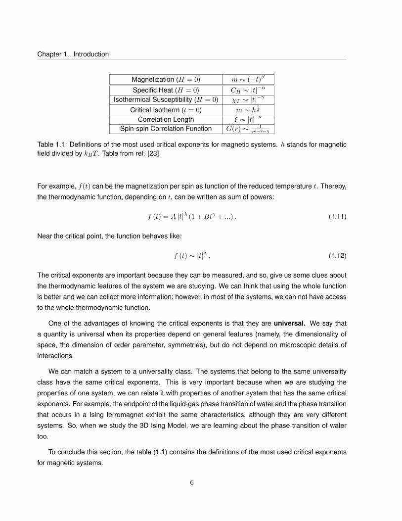
1.1 Definitions of the most used critical exponents for magnetic systems. h stands for mag-

netic field divided by kBT . Table from ref. [23]. . . . . . . . . . . . . . . . . . . . . . . . 6

4.1 Critical exponents for 2D and 3D Ising Model. d denotes dimensionality. From: [12], [18]. 57

iv

List of Figures

1.1 The blue dots were obtained using Monte Carlo simulations of a 2D Ising system for a

finite lattice 642 of size. The orange dots represent the theoretical result for the magneti-

zation for the 2D Ising model |m| ∼ (Tc − T )18 . . . . . . . . . . . . . . . . . . . . . . . . 2

1.2 The idea behind the OPE is that two operators sitting close together, as in the figure of

the left-hand side, are mapped to an effective operator just at one point under RG action,

as can be seen on the figure of the right-hand side. . . . . . . . . . . . . . . . . . . . . . 15

1.3 On the image of the left-hand side, we plot a series of horizontal and vertical lines that

intersect at right angles. After an inversion, around the origin, this image is mapped to

the right-hand side plot. Each line on the left-hand side is transformed to a circle. Notice,

however, that at the intersection points, the angles remain with π2 . . . . . . . . . . . . . . 17

1.4 Under an inversion, the interior of the sphere is mapped to the upper half space defined

by xd > 0. . . . . . . . . . . . . . . . . . . . . . . . . . . . . . . . . . . . . . . . . . . . 22

2.1 τCPU for absolute magnetization and for energy, depending on L, for 2D Ising Model,

using different algorithms: Wolff and Metropolis. It was used the Tc of 2D Ising Model.

The points are the experimental measurements and the dotted line is a power regression

of data. . . . . . . . . . . . . . . . . . . . . . . . . . . . . . . . . . . . . . . . . . . . . 29

2.2 τCPU for absolute magnetization and for energy, depending on L, for 3D Ising Model,

using different algorithms: Wolff and Metropolis. It was used the Tc of 3D Ising Model.

The points are the experimental measurements and the dotted line is a power regression

of data. . . . . . . . . . . . . . . . . . . . . . . . . . . . . . . . . . . . . . . . . . . . . . 30

3.1 Representation of the path of the walker. Notice that we normalize the positions by the

length (L) of the “box”. . . . . . . . . . . . . . . . . . . . . . . . . . . . . . . . . . . . . 34

3.2 Evolution with time for P (m, t|l, 0), with a box of L = 100 and p = 0.3, starting in l = L2 .

T is the number of steps of the walker. In this plot, we do not normalize the positions by

the size of the system. Therefore, pequilibirum = 0.01. . . . . . . . . . . . . . . . . . . . 37

v

List of Figures

3.3 Autocorrelation function. . . . . . . . . . . . . . . . . . . . . . . . . . . . . . . . . . . . 39

3.4 Autocorrelation time depending on the length of the box. . . . . . . . . . . . . . . . . . . 40

3.5 Left-hand side: Comparison between left-hand side and right-hand side of (3.42). Right-

hand side: using different number of points (m), proportional to τ , we get the distribution

of measurements of X1 (m). The data was obtained using a box of length L = 100 and

p = 0.3. . . . . . . . . . . . . . . . . . . . . . . . . . . . . . . . . . . . . . . . . . . . . 42

3.6 Left-hand side: validity of (3.47). Right-hand side: distribution of measurements of σ2,

using different values for m. This data was obtained using a box of length L = 100 and

p = 0.3. . . . . . . . . . . . . . . . . . . . . . . . . . . . . . . . . . . . . . . . . . . . . 45

3.7 Using different number of points (m), proportional to τ , we get the distribution of mea-

surements of k (m). The data was obtained using a box of length L = 100 and p = 0.3. . 49

3.8 The covariance between blocks B1 and B2, and the comparison with the right-hand side

of (3.70), using a box of L = 100 and p = 0.3. . . . . . . . . . . . . . . . . . . . . . . . . 51

3.9 Evolution of block’s errors. . . . . . . . . . . . . . . . . . . . . . . . . . . . . . . . . . . 54

4.1 Plots of energy, absolute magnetization, specific heat and susceptibility as function of β

for 2D Ising Model, using Monte Carlo Methods. . . . . . . . . . . . . . . . . . . . . . . 56

4.2 The Binder’s cumulant as function of β for 2D Ising model, using Monte Carlo Methods. . 56

4.3 Plots of energy, absolute magnetization, specific heat and susceptibility as function of β

for 3D Ising Model, using Monte Carlo Methods. . . . . . . . . . . . . . . . . . . . . . . 57

4.4 The Binder’s cumulant as function of β for 3D Ising model, using Monte Carlo Methods. . 58

4.5 FSS for absolute magnetization for 2D Ising Model. t, in the x-axis, denotes reduced

temperature. . . . . . . . . . . . . . . . . . . . . . . . . . . . . . . . . . . . . . . . . . 60

4.6 FSS for specific heat for 2D Ising Model. t, in the x-axis, denotes reduced temperature. . 61

4.7 FSS for susceptibility, for 2D Ising Model. t, in the x-axis, denotes reduced temperature. 62

4.8 FSS for absolute magnetization, for 3D Ising Model. t, in the x-axis, denotes reduced

temperature. . . . . . . . . . . . . . . . . . . . . . . . . . . . . . . . . . . . . . . . . . . 62

4.9 FSS for specific heat for 3D Ising Model. t, in the x-axis, denotes reduced temperature. . 63

4.10 FSS for susceptibility for 3D Ising Model. t, in the x-axis, denotes reduced temperature. 63

5.1 In this example we consider a two dimensional lattice with eleven points in each side.

Then, we consider a circle with radius of four lattice spacings. We count only the spins

that stay inside the disk. . . . . . . . . . . . . . . . . . . . . . . . . . . . . . . . . . . . 66

5.2 One point function of the operator ε (x) in the presence of a spherical boundary. . . . . . 66

5.3 Two point function of the local operators. . . . . . . . . . . . . . . . . . . . . . . . . . . . 67

vi

Chapter 1

Introduction

The goal of this chapter is to review the main concepts of critical phenomena in statistical systems and

of conformal field theory.

1.1 Phase transitions

Phase transitions are abrupt changes of physical observables, when the external fields, e. g., temper-

ature or pressure, are smoothly varied. The special values at which these changes occur are called

critical points. In the specific case of the temperature, we shall denote its critical value by Tc . In phase

transitions, there is a quantity that is zero in one of the sides of the transition, and it is different from zero

in the other side: it is the order parameter. The order parameter distinguishes the different phases of the

system and it is associated to a spontaneous symmetry breaking. The behavior of the local fluctuations

of the order parameter give us a way to characterize the nature of the transition.

There are two types of phase transitions. In first order (or discontinuous) phase transitions, as is

the case of liquid-gas transition in water, the order parameter is the density and it suffers a jump at the

critical point. In this case, a first derivative of the free energy of the system is discontinuous.

The other kind of phase transitions is the second order (or continuous) phase transition, e.g. 2D or

3D Ising ferromagnet and critical opalescence in water. The Ising ferromagnet models the interaction

of spins assuming each degree of freedom (i.e., the spin) interacts just with the nearest neighbor and it

has two possible states: the spin can be either up or down. The order parameter in this example is the

absolute value of the magnetization of the system. In this case, when T < Tc, the limits H → 0+ and

H → 0− (H denotes magnetic field) provide different values for the magnetization. This is an example of

the spontaneous symmetry breaking that we referred above: in spite of the Hamiltonian being invariant

under simultaneous reversal of all magnetic degrees of freedom, this symmetry is not respected by the

thermodynamic equilibrium state. At high temperatures the thermal fluctuations should dominate and

1

Chapter 1. Introduction

so, the order parameter should be zero in the thermodynamic limit. As the temperature is decreased,

the interactions of the system begin to be more important and at the critical temperature the absolute

magnetization starts to be non-zero. In this case, the order parameter varies continuously at the critical

point, as we can see in fig. (1.1). The relation between the magnetization and the temperature, for 2D

Ising model, near the critical temperature, is given by |m| ∼ (T − Tc)18 , as we will see in sections below.

This type of scaling between two measurable quantities is universal to several systems, even if the

microscopic description of each of the systems differ (we will refer an explanation for this phenomenon

when we discuss the renormalization group, in section 1.5 ). At the critical point, there are correlations

of all distances between the degrees of freedom and the correlation length 1 becomes infinite. Thus,

the strong correlations between a large number of degrees of freedom makes the study of second order

phase transitions more complicated, in general. However, there are techniques developed to study

critical phenomena. One of them is the renormalization group.

0 1 2 3 4T

0.2

0.4

0.6

0.8

1.0

1.2

m

MonteCarlo

(T-Tc)1

8

Figure 1.1: The blue dots were obtained using Monte Carlo simulations of a 2D Ising system for a finitelattice 642 of size. The orange dots represent the theoretical result for the magnetization for the 2D Isingmodel |m| ∼ (Tc − T )

18 .

1.2 Correlation length and correlation function

One of the most important quantities that features a system is the correlation length. The correlation

length, usually represented by ξ, is the distance over which the fluctuations of microscopic degrees

of freedom - such as the directions of spins, for example - in one region of space are influenced (or

1The correlation length ξ measures the range of the correlation function. A more detailed explanation about correlationlength and correlation function will be given in the next sections.

2

1.2. Correlation length and correlation function

correlated with) by fluctuations in another region. If the distance between two spins is larger than this

length, we can say that they are practically uncorrelated, because their fluctuations will not affect each

other significantly.

In first order phase transitions, the correlation length is finite at the transition temperature, while in

second order phase transitions, the correlation length becomes infinite, i.e., diverges, which means that

points far apart become correlated.

An important observable in critical phenomena is the correlation function. This function measures

how the microscopic variables at different positions are correlated. In other words, it measures the order

of the system. The correlation function is positive if the values of those variables fluctuate in the same

direction, and it is negative if they fluctuate in opposite directions. It takes zero value if the fluctuations

are uncorrelated. The connected correlation function of n-points, G(n)c (i1, i2, i3..., in), is defined by:

G(n)c (i1, i2, i3, ..., iN ) ≡ G(n) −

∑partitions

product of G(m)c , withm < n (1.1)

where iN is the position of a local observable of the system and G(n) is the whole n-point correlation

function. One example is the two-point correlation function between spins at sites i and j:

G(2)(i, j) = 〈(si − 〈si〉) (sj − 〈sj〉)〉 . (1.2)

If the system is translationally invariant, the correlation function only depends on the difference between

positions i and j. Moreover, if the system is also isotropic, the function only depends on the distance

between spins i and j, |i− j|. In the theory of critical phenomena, one is often interested in isotropic

lattices and, therefore, it is usual consider G(2) only function of |i− j|. Thereby, (1.2) can be rewritten

as:

G(2)(r) ≡ 〈sisj〉 − 〈si〉 2, (1.3)

where r ≡ |i− j|.The correlation function should also depend on the correlation length since it measures how the

degrees of freedom are separated. Generically, the two point function decays exponentially over large

distances.

In second order phase transitions, if the system is not at Tc, the spins become uncorrelated as r

increases and the correlation function decays to zero exponentially:

G(2)(r) ∼ r−τe−r/ξ, (1.4)

where τ is some number and ξ is the correlation length.

At the critical point, the correlation length becomes infinite and eq. (1.4) does not work. From

3

Chapter 1. Introduction

experiments and exactly soluble models, the correlation function decays as power law:

G(2)(r) ∼ 1

rd−2+η, (1.5)

where d is the dimensionality of the system and η is a critical exponent. We will define and explore the

critical exponents in section 1.4.

1.3 Brief summary of Ising Model

The goal of the Ising model is to describe the simplest possible interaction between a system of spins.

For the one dimensional case the Ising model is exactly solvable, even in the presence of a magnetic

field. However, it does not possess a phase transition at finite temperature. So, it is not the most

interesting case for studying critical phenomena. In higher dimensions, the Ising model has a phase

transition, but solving the problem becomes harder. The 2D Ising Model without magnetic field has an

analytical solution, which was achieved by Lars Onsager in 1944 [2], however, the analytical solution for

the case H 6= 0 has not been discovered yet. For higher dimensions, there is no analytical solution and

in the particular case of the Ising in three dimensions we usually resort to numerical studies2 to access

the physical quantities.

The Ising model works in this way: we have a set of spins that interact with first neighbors. This

system can be in a magnetic field. To simplify, we will consider, in this study, that there is no magnetic

field. In this case, the Hamiltonian is:

H = J

N∑〈ij〉

(1− σiσj), (1.6)

in which 〈ij〉 stands for nearest neighbors, σi is the spin at position i and can take two possible values:

+1 or −1 (representing the spin “up” or “down”) and J is the constant interaction between spins (we

suppose that it does not depend on site; however, in most general cases, it can depend, and we have a

constant Ji,j for each pair σiσj).

The order parameter is the absolute magnetization of the system per spin (see section 1.1 for the

meaning of order parameter ):

|m| = 1

N

∣∣∣∣∣∑i

σi

∣∣∣∣∣ , (1.7)

where N is the total number of spins. This sum is over all points of the lattice.

2Even if the Ising model for three dimensions is not known it is still possible to extract information analytically using approx-imations. In this context we mention the ε and the high temperature expansions.

4

1.4. Critical Exponents and Universality

For T > Tc, the system is in paramagnetic phase (disordered spins, more symmetric phase) and for

T < Tc, the system is in ferromagnetic phase ( ordered spins, less symmetric phase). When T = Tc,

regions that are ferromagnetic and other that are paramagnetic coexist together. Here, the correlation

length is infinite; if we have a finite sample, it will be restricted by the linear length of the system, L.

Thus, for a finite system, there is no phase transition. In fact, it is easy to understand: phase transitions

are characterized by divergence when the temperature is varied smoothly. However, all thermodynamic

quantities can be obtained from the partition function that, naively, is a completely regular function of

the temperature T . Remember that the partition function is given by a sum over all states of the factor

e−βE (β is 1kBT

, where kB is the Boltzmann constant, and E is the energy of the system) and it is only

because there is an infinite number of terms that the sum can get a divergence as a function of T . In the

one dimensional Ising model, there is no phase transition at finite temperature. The critical temperature

for the 2D Ising model is

Tc =2J

ln(1 +√

2) . (1.8)

The main goal of this work is to study the critical point of the three dimensional Ising model using Monte

Carlo methods. We will use J = 1 and set kB = 1. In this numerical approach, we will not be able

to simulate an infinite system, so we know before hand that there is no critical point in the particular

case we are dealing. However, it is possible to extract the information of the observables of the critical

Ising model by analyzing how the finite system scales with size; this is called finite size scaling. We will

discuss it in chapter 4.

1.4 Critical Exponents and Universality

As described before, the two point function in a critical system decays as a power law. The exponent of

the power is one example of critical exponent. More concretely, they describe the behavior of physical

observables, such as specific heat or magnetic susceptibility, when the external fields are varied near

the critical point. Let us consider a function f that depends on t. Then, the critical exponent is defined

by:

λ = limt→0

ln |f (t)|ln |t|

, (1.9)

where t is the reduced temperature, defined by:

t =T − TcTc

. (1.10)

5

Chapter 1. Introduction

Magnetization (H = 0) m ∼ (−t)β

Specific Heat (H = 0) CH ∼ |t|−α

Isothermical Susceptibility (H = 0) χT ∼ |t|−γ

Critical Isotherm (t = 0) m ∼ h1δ

Correlation Length ξ ∼ |t|−ν

Spin-spin Correlation Function G(r) ∼ 1rd−2−η

Table 1.1: Definitions of the most used critical exponents for magnetic systems. h stands for magneticfield divided by kBT . Table from ref. [23].

For example, f(t) can be the magnetization per spin as function of the reduced temperature t. Thereby,

the thermodynamic function, depending on t, can be written as sum of powers:

f (t) = A |t|λ (1 +Btγ + ...) . (1.11)

Near the critical point, the function behaves like:

f (t) ∼ |t|λ , (1.12)

The critical exponents are important because they can be measured, and so, give us some clues about

the thermodynamic features of the system we are studying. We can think that using the whole function

is better and we can collect more information; however, in most of the systems, we can not have access

to the whole thermodynamic function.

One of the advantages of knowing the critical exponents is that they are universal. We say that

a quantity is universal when its properties depend on general features (namely, the dimensionality of

space, the dimension of order parameter, symmetries), but do not depend on microscopic details of

interactions.

We can match a system to a universality class. The systems that belong to the same universality

class have the same critical exponents. This is very important because when we are studying the

properties of one system, we can relate it with properties of another system that has the same critical

exponents. For example, the endpoint of the liquid-gas phase transition of water and the phase transition

that occurs in a Ising ferromagnet exhibit the same characteristics, although they are very different

systems. So, when we study the 3D Ising Model, we are learning about the phase transition of water

too.

To conclude this section, the table (1.1) contains the definitions of the most used critical exponents

for magnetic systems.

6

1.5. Renormalization Group Transformation

1.5 Renormalization Group Transformation

One is often interested in observables which vary smoothly or, in other words, in the long wave length. In

this context, it is not hard to believe that fine details of the microscopic interaction do not alter significantly

long range effects. The renormalization group tries to study how a given model, i.e., the Hamiltonian

or Lagrangian, gives rise to large distance physics. The philosophy of the method is simple. Let us

consider a system with many degrees of freedom distributed over space. Now, we just try to integrate

the degrees of freedom which are a given distance apart. In the case that the renormalization group is

done in real space and in a spin lattice system, we can view this as summing over a given set of spins

and rescale the lattice size at the end. This rescaling is important, as we will be trying to compare the

original and transformed interactions. This is a process that can be done repeatedly, generating a flow in

the space of all possible Hamiltonians or Lagrangians. The endpoint of this flow is called the fixed point.

Let us remark that it is possible that two nearby Hamiltonians in this space of all possible interactions will

land on the same fixed point. This is nothing more than what was called universality. Implementations

of the renormalization group often involve approximations that if well made do not affect the end results.

Let us be more concrete and consider an Hamiltonian H, and denote the action of the renormalization

group as

H′ = RH, (1.13)

in which H′ is the renormalized Hamiltonian of the new system and R is the renormalization group op-

erator. This operation decreases the number of degrees of freedom from N to N ′. The renormalization

transformation can be done in real space, by removing or grouping spins, or in momentum space, by

integrating out large wavevectors. The scale factor of the transformation, b, is defined by:

bd =N

N ′, (1.14)

where d is the dimensionality of the space. In the following we will present a detailed analysis of the

action of the renormalization group in the space of all possible interactions. We will conclude that some

interactions are relevant, i.e., they determine which fixed point the system will approach, and other are

irrelevant. In the next subsection we show a general example of the renormalization group to make the

transition to the theory more smooth.

1.5.1 The Block Spin Transformation

In this section we will present an example of a particular renormalization group scheme, called block

spin transformation. For concreteness, consider a spin system over a d- dimensional lattice with spacing

7

Chapter 1. Introduction

a. The whole purpose of RG is to integrate over short degrees of freedom, in this case, divide the lattice

in blocks, say of size l × l · · · × l, containing ld spins, and sum over all the spins in each block except

one. Then we would be left with an effective interaction for the representative spin of the renormalized

block. One such scheme is the block spin transformation where for the representative of the spin of a

block we take the majority rule. For this purpose, one defines the function:

T(s′; s1, ..., sld

)=

1, s′∑

i si > 0;

0 otherwise. (1.15)

The Hamiltonian describing the interactions of new spin is defined by:

exp(−H′

(s′))≡ Trs

∏blocks

T(s′; si

)exp (−H (s)) , (1.16)

Consider that we have a lattice of spins, whose partition function is:

Z = Trs exp(−H(s)), (1.17)

(the β constant was absorbed into the definitions of the parameters of H). Notice that the partition

function computed with the new Hamiltonian or with the old one are the same:

Trs′e−H′(s′) = Trse−H(s), (1.18)

where we have used∑

s′ T (s′; si) = 1. Moreover, the new Hamiltonian preserves not just the partition

function but also all the physics whose wave length is considerably larger than the typical size of the

block. This will be important to study how correlation functions transform under RG action. However,

this method is not practical in most cases and more approximations must be done to carry on the

computation.

1.6 Scaling variables, Scaling Function and Critical Exponents

The goal of this section is to explain the theory behind the renormalization group (RG), applying the

ideas present in the last subsection to the space of all couplings. In the following we shall denote by

K this space, then the action of the renormalization group relates the couplings of the transformed

system RH to the original one,

K ′ = R(K), (1.19)

8

1.6. Scaling variables, Scaling Function and Critical Exponents

where R depends on the specific transformation chosen and on the parameter b. This equation tells

us that the couplings of the new system are obtained by combinations of the original. Again, this is a

process that can be done iteratively and will generate a path in the space of all possible couplings. The

fixed point in this path is defined by the condition

K∗ = RK∗. (1.20)

The operation R depends on the scale b and in principle we can set this scale to be arbitrarily close to

1, b = 1 + δ. Close to a fixed point we can write the following system of equations:

K ′a −K∗a '∑b

Tab (Kb −K∗b) , (1.21)

where we used Tab = ∂K′a

∂Kb|K=K∗ . This matrix tells how is the behavior of the renormalization group

near the fixed point. By definition, Tab does not have to be symmetric and in general it is not. Let us

represent the eigenvalues of T by λi and the left eigenvectors as ei3,

∑a

eiaTab = λieib. (1.22)

There is a specific linear combination of Ka −K∗a such that it is an eigenvector of the renormalization

group, to this specific linear combination of variables we call scaling variables. More rigorously, they

are defined in the following way:

ui =∑a

eia (Ka −K∗a) . (1.23)

From (1.21), (1.22) and (1.23) we can easily check that, near the fixed point, scaling variables transform

multiplicatively or, in other words, they are eigenvectors of the RG action:

u′i =∑a

eia(K′a −K∗a)

= λiui. (1.24)

The renormalization group action depends on the scale factor b and so the eigenvalues must also

have this dependence. Since the correlations in critical systems are characterized by power laws it is

convenient to write the eigenvalues λi as

λi = byi , (1.25)

where the variable yi is related with the critical exponents, as we will see soon.

3Remember that in the case where the a matrix is not symmetric the right and left eigenvectors do not need to be the same.

9

Chapter 1. Introduction

When yi > 0, ui is relevant; it means that applying renormalization group transformations several

times will move ui away from the fixed point. If yi < 0, ui is irrelevant, that is, applying renormalization

group transformations several times will approximate ui to the fixed point. Finally, if yi = 0, ui is

marginal, i.e., we do not know, by linearized equations (1.21), if ui is moving away from the fixed point

or towards it.

The Ising Model has two relevant scaling variables: a thermal scaling variable, ut, with eigenvalue

yt and a magnetic scaling variable, uh, whose eigenvalue is yh. Near the critical point, ut and uh are

proportional to t (temperature) and h (magnetic field), respectively. When t = 0 and h = 0, ut and uhvanish. So, we have the following relations:

ut =t

t0+O

(t2, h2

)(1.26)

uh =h

h0+O

(th, h3

), (1.27)

in which t0 and h0 are constants (non-universal).

It is possible to get the free energy per spin, as function of the couplings K:

f (K) = − 1

Nln (Z) . (1.28)

Under renormalization, and if K does not include a constant in Hamiltonian, the free energy f (K)transforms inhomogeneously:

f (K) = g (K) + b−df(K ′). (1.29)

This is the fundamental transformation equation for the free energy. It is easy to verify that free

energy transforms inhomogeneously when one applies renormalization. Nevertheless, for obtaining

the critical exponents, we are only interested in the singular part of the free energy, that is constituted

merely by f . We can neglect the term g (K), assuming that it comes from summing over the short

wavelength degrees of freedom. For that reason, g is an analytic function of K everywhere.

Therefore, the transformation law for the singular part of the free energy is:

fs (K) = b−dfs(K ′). (1.30)

Near the fixed point, we can write (1.30) as function of the scaling variables:

fs(ut, uh) = b−dfs(bytut, b

yhuh). (1.31)

10

1.6. Scaling variables, Scaling Function and Critical Exponents

And if we iterate the renormalization group n times, we get:

fs (ut, uh) = b−ndfs (bnytut, bnyhuh) . (1.32)

We have to be careful with the number of iterations, once that ut and uh increase as we increase the

number of iterations. If n is too big, the linear approximation to the renormalization group equations can

not be valid. To control this problem, we stop the iteration when we get the condition:

|bnytut| = ut0 , (1.33)

in which ut0 is arbitrary and it is small enough to allow the approximation. Thus,

fs (ut, uh) =

∣∣∣∣ utut0∣∣∣∣ dyt fs

(±ut0 , uh

∣∣∣∣ utut0∣∣∣∣−

yhyt

). (1.34)

Rewriting the last expression, using (1.26) and (1.27), we see that ut0 can be embedded into a redefini-

tion of the scale factor t0, and so

fs (t, h) =

∣∣∣∣ tt0∣∣∣∣ dyt Φ

(h/h0

|t/t0|yhyt

). (1.35)

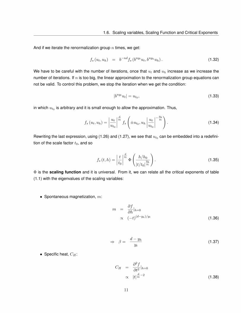
Φ is the scaling function and it is universal. From it, we can relate all the critical exponents of table

(1.1) with the eigenvalues of the scaling variables:

• Spontaneous magnetization, m:

m =∂f

∂h|h=0

∝ (−t)(d−yh)/yt (1.36)

⇒ β =d− yhyt

(1.37)

• Specific heat, CH :

CH =∂2f

∂t2|h=0

∝ |t|dyt−2 (1.38)

11

Chapter 1. Introduction

⇒ α = 2− d

yt(1.39)

• Magnetic susceptibility, χH :

χH =∂2f

∂h2|h=0

∝ |t|(d−2yh)

yt (1.40)

⇒ γ = −(d− 2yh)

yt(1.41)

• Magnetization with H 6= 0:

m =∂f

∂h

=

∣∣∣∣ tt0∣∣∣∣d−yhyt

Φ′

h/h0∣∣∣ tt0 ∣∣∣ yhyt (1.42)

In this case, in order to m have a finite limit as t → 0, the function Φ′(x) must behave like a

power of x as x → ∞. Let us say that when x → ∞, Φ′(x) → xa. Now, we can substitute this

expression in (1.42), and we verify that a = d−yhyh

so that m be finite when t → 0. Therefore, we

obtain:

m ∝ hd−yhyh (1.43)

⇒ δ =yh

(d− yh). (1.44)

1.7 Correlation function of scaling operators

The action of the renormalization group maps one set of couplings from a given Hamiltonian to a new

set of couplings. This is done by integrating some of the degrees of freedom, so computing the partition

function using the original or renormalized Hamiltonian should give the same result,

Z =∑si

e−βH =∑s′i

e−βH′. (1.45)

12

1.7. Correlation function of scaling operators

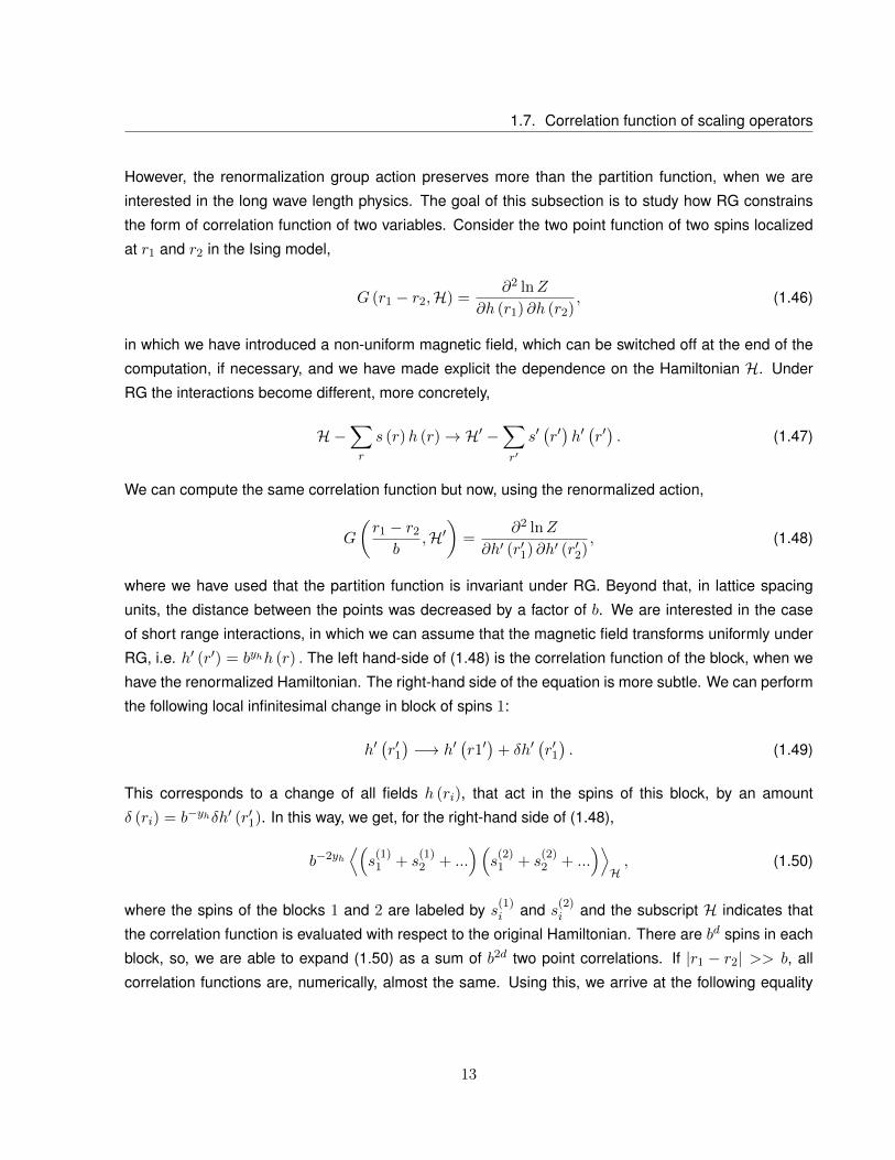
However, the renormalization group action preserves more than the partition function, when we are

interested in the long wave length physics. The goal of this subsection is to study how RG constrains

the form of correlation function of two variables. Consider the two point function of two spins localized

at r1 and r2 in the Ising model,

G (r1 − r2,H) =∂2 lnZ

∂h (r1) ∂h (r2), (1.46)

in which we have introduced a non-uniform magnetic field, which can be switched off at the end of the

computation, if necessary, and we have made explicit the dependence on the Hamiltonian H. Under

RG the interactions become different, more concretely,

H−∑r

s (r)h (r)→ H′ −∑r′

s′(r′)h′(r′). (1.47)

We can compute the same correlation function but now, using the renormalized action,

G

(r1 − r2

b,H′)

=∂2 lnZ

∂h′ (r′1) ∂h′ (r′2), (1.48)

where we have used that the partition function is invariant under RG. Beyond that, in lattice spacing

units, the distance between the points was decreased by a factor of b. We are interested in the case

of short range interactions, in which we can assume that the magnetic field transforms uniformly under

RG, i.e. h′ (r′) = byhh (r) . The left hand-side of (1.48) is the correlation function of the block, when we

have the renormalized Hamiltonian. The right-hand side of the equation is more subtle. We can perform

the following local infinitesimal change in block of spins 1:

h′(r′1)−→ h′

(r1′)

+ δh′(r′1). (1.49)

This corresponds to a change of all fields h (ri), that act in the spins of this block, by an amount

δ (ri) = b−yhδh′ (r′1). In this way, we get, for the right-hand side of (1.48),

b−2yh⟨(s

(1)1 + s

(1)2 + ...

)(s

(2)1 + s

(2)2 + ...

)⟩H, (1.50)

where the spins of the blocks 1 and 2 are labeled by s(1)i and s(2)

i and the subscript H indicates that

the correlation function is evaluated with respect to the original Hamiltonian. There are bd spins in each

block, so, we are able to expand (1.50) as a sum of b2d two point correlations. If |r1 − r2| >> b, all

correlation functions are, numerically, almost the same. Using this, we arrive at the following equality

13

Chapter 1. Introduction

relating the original and transformed correlation function:

G

(r1 − r2

b,H′)

= b2(d−yh)G (r1 − r2,H) , (1.51)

Now, we can simply set the magnetic field to zero and we get:

G (r, t) = b−2(d−yh)G(rb, bytt

), (1.52)

where we have assumed that the system is rotation invariant and, for convenience, setting |r1 − r2| = r.

Such as we did in (1.32), we can iterate (1.52) n times. In this case, we stop the iteration at bnyt(tt0

)=

1. Therefore, we get:

G(r, t) =

∣∣∣∣ tt0∣∣∣∣

2(d−yh)yt

Ψ

(r

|t/t0|− 1yt

). (1.53)

For large r, as we already referred, G ∼ exp(−rξ ). As stated in Table (1.1), ξ ∼ |t|−ν . We can identify

ξ ∼ |t|−1yt in (1.53). Therefore, we obtain the following relation:

ν =1

yt. (1.54)

At the critical point, t = 0, this equation tells us that the correlation function should decay as

G (r, 0) ∝ r−2(d−yh). (1.55)

Thus, the decay of this correlation function at criticality is determined by renormalization group eigen-

value yh.

We will now move to correlation functions of other fields. Recall that the scaling variable ui can

be written in terms of the coupling Ki − K∗i . These interactions are associated with fields Si in the

Hamiltonian. Scaling operators φi are defined by,∑i

uiφi =∑a

(Ka −K∗a)Sa. (1.56)

By promoting the variables to have a space position ui (r), we can mimic almost exactly the same

derivation for correlation functions of two operators φi:

〈φi (r1)φj (r2)〉 ∝ r−2(d−yi). (1.57)

Let us just emphasize that, given a product of local operators, they will not be, in general, scaling

operators and, consequently, their correlation function will not have this simple power law decay.

14

1.8. Conformal and scale invariant field theories

RGx1 x2

x1'

Σkk '

21

Figure 1.2: The idea behind the OPE is that two operators sitting close together, as in the figure of theleft-hand side, are mapped to an effective operator just at one point under RG action, as can be seenon the figure of the right-hand side.

1.7.1 Operator Product Expansion

The goal of this subsection is to introduce the concept of operator product expansion (OPE), that is

ubiquitous in statistical physics and quantum field theory. Consider a lattice system with two fields

located at points x1 and x2. Then, under a typical RG action, these points can be transformed into one,

which we denote by x′1. Thus, in the original system, there were two fields at different points. However,

under RG these were mapped to single effective field - fig.(1.2).

In the vicinity of a critical point we can think that these operators are scaling fields, more concretely,

we have one operator φ1 at point x1 and another operator φ2 at point x2. These operators can be

expressed in terms of the product local fields Sa . Under RG action this product will be mapped to a

different set of fields, say S′a, but at a single point. Then, we can rewrite these new fields in terms of

scaling operators∑

k φk. Thus, we conclude that generically we have

φ1 (x1)φ2 (x2)→∑k

φk (x1) . (1.58)

This is valid as long as there are no other operators in the neighborhood of these two operators and

when it is evaluated inside a given correlation function. As we will see in the following section, the OPE

is an identity which is extremely important in the context of conformal field theories.

1.8 Conformal and scale invariant field theories

The action of the renormalization group changes the system size, integrating out all degrees of freedom

which are shorter than a specified cut-off. The critical point is a fixed point in this action, so the system at

this special point is not changed under the RG action. Thus, at the critical point, we are interested in the

long wave length interactions, i.e., with continuous description. By definition, the fixed point should have

15

Chapter 1. Introduction

an additional symmetry, namely it is invariant under scale transformations. Scale invariant theories,

sometimes, get their symmetry enlarged to conformal symmetry (translations, dilations, rotations and

special conformal transformations, that we will explain in the next subsection). This amounts to having

also inversion symmetry. The necessary and sufficient conditions to have this enlargement of symmetry

in a field theory are not completely understood yet. In 2D it was proved that this is the case, i.e., once

the system is scale invariant and unitary it is also conformal invariant. In higher dimensions, it was

recently proved just for d = 4 [19].

The 3D Ising model at the critical temperature is obviously scale invariant. One of the main goals of

this thesis is to verify if, in the continuum limit, this theory is also conformal invariant. For this purpose,

we will look for specific signatures of conformal symmetry that are not implied by scale symmetry. So

we will begin by explaining the basic properties of the conformal symmetry and then we will analyze

a system with boundary. In the presence of a boundary, there is a substantial difference between

conformal and scale symmetry.

1.8.1 Conformal Transformations

A conformal field theory has the following symmetries:

• translations:

(x′)µ

= xµ + aµ; (1.59)

• dilations: (x′)µ

= αxµ; (1.60)

• rotations: (x′)µ

= Mµν x

ν (1.61)

• inversions: (x′)µ

=xµ

x2(1.62)

• special conformal transformation, SCT, that is a inversion followed by a translation that, in turn, is

followed by another inversion:

(x′)µ

=xµ − bµx2

1− 2b.x+ b2x2(1.63)

=xµ

x2 − bµ(xµ

x2 − bµ)2 (1.64)

16

1.8. Conformal and scale invariant field theories

xμ→

xμ

x2

Figure 1.3: On the image of the left-hand side, we plot a series of horizontal and vertical lines that inter-sect at right angles. After an inversion, around the origin, this image is mapped to the right-hand sideplot. Each line on the left-hand side is transformed to a circle. Notice, however, that at the intersectionpoints, the angles remain with π

2 .

The inversion symmetry is not connected to the identity, so it is usual to introduce the connected part

of the conformal group by replacing the generator of inversions by special conformal transformations

generator, Kµ, defined by,

Kµ = IPµI,

where Pµ denotes translations and I an inversion.

The conformal group is associated with the symmetries that preserve angles. It is obvious that

translations, rotations and dilations preserve the angle between two intersecting lines. In fig. (1.3) we

plot an example of inversion symmetry and we verify that it preserves the angles too.

1.8.2 Correlation functions

Operators belonging to a conformal field theory are of one of two types, they are either primary or they

are descendants. The distinction between the two is: a primary operator is killed by the action of the

generator of the special conformal transformations, Kµ

Kµ |O〉 = 0, (1.65)

where |O〉 ≡ O (0) |0〉; in turn, the descendants operators are obtained from the primary operator just

by acting with the generator of translations, Pµ:

iPµ |O〉 = ∂µO (0) |0〉 , (1.66)

17

Chapter 1. Introduction

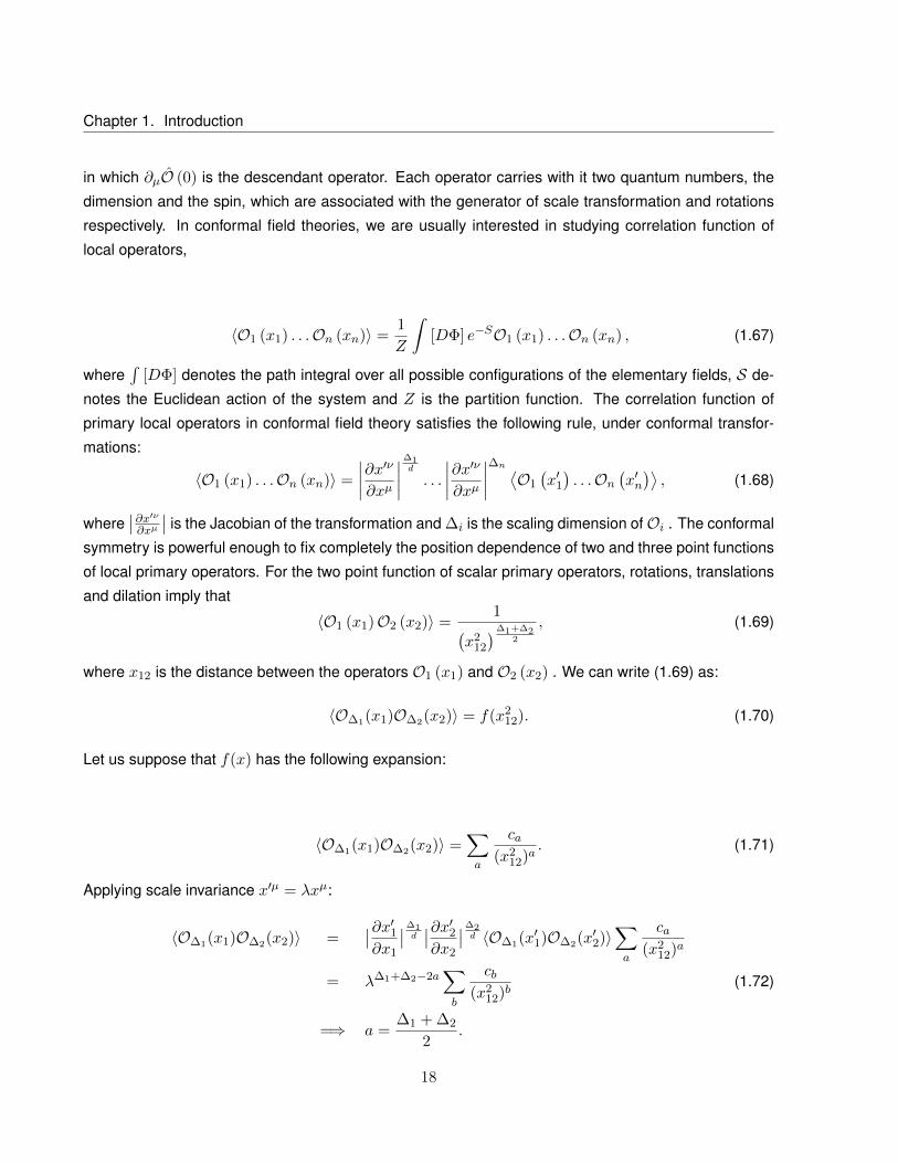
in which ∂µO (0) is the descendant operator. Each operator carries with it two quantum numbers, the

dimension and the spin, which are associated with the generator of scale transformation and rotations

respectively. In conformal field theories, we are usually interested in studying correlation function of

local operators,

〈O1 (x1) . . .On (xn)〉 =1

Z

ˆ[DΦ] e−SO1 (x1) . . .On (xn) , (1.67)

where´

[DΦ] denotes the path integral over all possible configurations of the elementary fields, S de-

notes the Euclidean action of the system and Z is the partition function. The correlation function of

primary local operators in conformal field theory satisfies the following rule, under conformal transfor-

mations:

〈O1 (x1) . . .On (xn)〉 =

∣∣∣∣∂x′ν∂xµ

∣∣∣∣∆1d

. . .

∣∣∣∣∂x′ν∂xµ

∣∣∣∣∆n ⟨O1

(x′1). . .On

(x′n)⟩, (1.68)

where∣∣∂x′ν∂xµ

∣∣ is the Jacobian of the transformation and ∆i is the scaling dimension ofOi . The conformal

symmetry is powerful enough to fix completely the position dependence of two and three point functions

of local primary operators. For the two point function of scalar primary operators, rotations, translations

and dilation imply that

〈O1 (x1)O2 (x2)〉 =1(

x212

)∆1+∆22

, (1.69)

where x12 is the distance between the operators O1 (x1) and O2 (x2) . We can write (1.69) as:

〈O∆1(x1)O∆2(x2)〉 = f(x212). (1.70)

Let us suppose that f(x) has the following expansion:

〈O∆1(x1)O∆2(x2)〉 =∑a

ca(x2

12)a. (1.71)

Applying scale invariance x′µ = λxµ:

〈O∆1(x1)O∆2(x2)〉 =∣∣∂x′1∂x1

∣∣∆1d∣∣∂x′2∂x2

∣∣∆2d 〈O∆1(x′1)O∆2(x′2)〉

∑a

ca(x2

12)a

= λ∆1+∆2−2a∑b

cb(x2

12)b(1.72)

=⇒ a =∆1 + ∆2

2.

18

1.8. Conformal and scale invariant field theories

Notice that, under inversions, we have

x′212 =x2

12

x21x

22

,∣∣∂x′∂x

∣∣ =1

(x2)d. (1.73)

Therefore, we have:

〈O∆1(x1)O∆2(x2)〉 =1

(x212)

∆1+∆22

=∣∣∂x′1∂x1

∣∣∆1d∣∣∂x′2∂x2

∣∣∆2d 〈O∆1(x′1)O∆2(x′2)〉 (1.74)

⇒ 1

(x212)

∆1+∆22

=∣∣∂x′1∂x1

∣∣∆1d∣∣∂x′2∂x2

∣∣∆2d

(x21x

22)

∆1+∆22

(x212)

∆1+∆22

=1

(x21)∆1(x2

2)∆2

(x21x

22)

∆1+∆22

(x212)

∆1+∆22

which implies that the two point function is non-zero only if ∆1 = ∆2. For the three point function of

scalar primary operators, we have

〈O1 (x1)O2 (x2)O3 (x3)〉 =C123(

x212

)∆1+∆2−∆32

(x2

13

)∆1+∆3−∆22

(x2

23

)∆2+∆3−∆12

. (1.75)

Notice that we are always free to choose a normalization such that the two point function is normalized

to one. However, if this is done, the coefficient appearing in the three point function is uniquely fixed. An

important property of conformal field theories is the OPE expansion,

O2 (x2)O1 (x1) =∑k

C12kB (x12, ∂x1)Ok (x1) , (1.76)

where the product of two operators at different points can be replaced by a sum over operators located

at a single point. The function B (y, z) can be determined by requiring consistency of the OPE and the

explicit result for two and three point functions. This is an operator identity that can be successively

used in correlation functions, turning an n-point function into a sum of (n − 1)-point functions. From

what has been said above, we conclude that all information in a conformal field theory is encoded in

two and three point functions. In the present work we will be interested mostly in correlation functions

of scalar primary operators.

19

Chapter 1. Introduction

1.8.3 Weyl invariance

A theory is said to have Weyl symmetry if it stays invariant under a Weyl transformation:

gab (x) = λ (x) g′ab (x) , (1.77)

where gab and g′ab are metrics. Notice that this type of transformation leaves the angles between two

intersecting lines unchanged. Let us denote by 〈. . . 〉g the correlation function of a theory having the

metric g. Then, the correlation functions of operators that are related through a Weyl transformation

satisfy

〈O (x1) . . .O (xn)〉g =⟨O(x′1). . .O

(x′n)⟩g′

(1.78)

=

∣∣∣∣∂x′∂x

∣∣∣∣∆1d

x=x1

. . .

∣∣∣∣∂x′∂x

∣∣∣∣∆nd

x=xn

⟨O(x′1). . .O

(x′n)⟩g′, (1.79)

where x′ denotes the coordinates in the system with metric g′ab , O are primary operators and d is the

dimensionality of the system. This is the Weyl invariance. In this way, we can relate correlation functions

having metrics which are Weyl related.

1.8.4 Boundary conformal field theory - planar boundary

The presence of a boundary in a conformal field theory breaks the symmetry of the system. Then, it

is expected that the system is not so constrained. The simplest boundary that one can engineer in a

conformal field theory is a planar boundary. Let us consider a system that exists only for xd ≥ 0, with

xd being coordinate in a d dimensional theory. The symmetry is reduced in this case; for example, it is

only invariant under rotations that preserve the boundary. In this case, the symmetry does not exclude

one point functions. For instance, we have

〈O (x)〉 =a

(xd)∆, (1.80)

where a is a constant.

Correlation functions involving two operators are not completely determined by symmetry. We can

understand this fact easily by noticing that the variable

ζ =(x− y)2

xdyd(1.81)

is left invariant under scale transformations. ζ is called cross ratio. So, we conclude that the two point

function in the presence of the boundary is given by:

20

1.8. Conformal and scale invariant field theories

〈O1 (x)O2 (y)〉 =g (ζ)(

(x− y)2)∆1+∆2

2

, (1.82)

with g an undetermined function of the conformal cross ratio ζ. However, in the limit in which the points

are coming close together, ζ → 0, we know that the function g (ζ) should go to 1 if O1 = O2. This

makes sense because in this limit the operators do not feel the presence of the boundary.

In the presence of the boundary, we have another type of OPE, namely the bulk-to-boundary OPE. In

this case, we can replace an operator, that is a small distance apart from the boundary, by a combination

of operators living on the boundary

O1 (x) =1

x∆1−∆kd

∑k

a∆kD (xd, ∂xd) Ok (~x) , (1.83)

where we have used the notation ~x = (x1, . . . , xd−1, 0). Ok (~x) are operators living on the boundary with

scaling dimension ∆k, the constants a∆kare new physical numbers (introduced by the presence of the

boundary) and the functionD (xd, ∂xd) encodes the contribution of the descendants operators. Now, we

can try to take the limit in which the points of the two point function (1.82) are approaching the boundary.

The leading order contribution will be given by the boundary operators with lowest dimension. Notice

that for this derivation we have used that two point function of boundary operators, O, is completely

determined by conformal symmetry. The reason is simple to understand: since these operators are

located at the boundary, it is like they are effectively in a d− 1 system, with conformal symmetry and no

boundary.

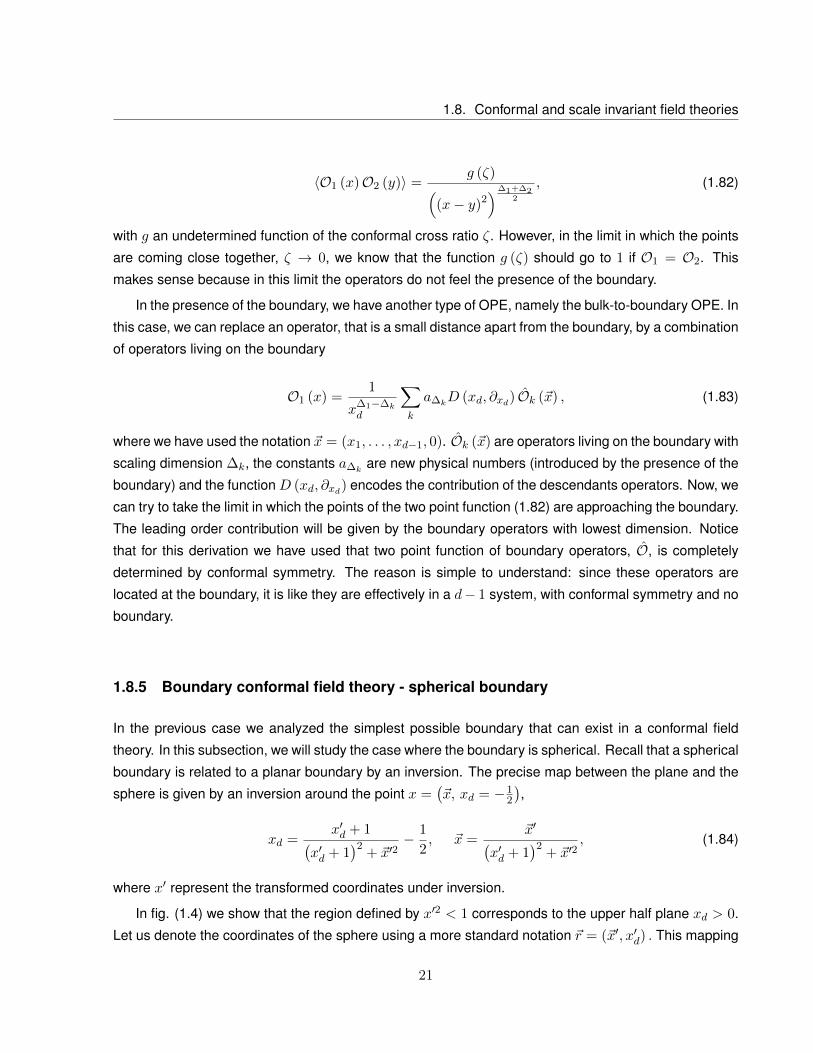
1.8.5 Boundary conformal field theory - spherical boundary

In the previous case we analyzed the simplest possible boundary that can exist in a conformal field

theory. In this subsection, we will study the case where the boundary is spherical. Recall that a spherical

boundary is related to a planar boundary by an inversion. The precise map between the plane and the

sphere is given by an inversion around the point x =(~x, xd = −1

2

),

xd =x′d + 1(

x′d + 1)2

+ ~x′2− 1

2, ~x =

~x′(x′d + 1

)2+ ~x′2

, (1.84)

where x′ represent the transformed coordinates under inversion.

In fig. (1.4) we show that the region defined by x′2 < 1 corresponds to the upper half plane xd > 0.

Let us denote the coordinates of the sphere using a more standard notation ~r = (~x′, x′d) . This mapping

21

Chapter 1. Introduction

Figure 1.4: Under an inversion, the interior of the sphere is mapped to the upper half space defined byxd > 0.

corresponds to a Weyl transformation, so the correlation functions can be written as:

〈O (~r)〉 =a(

1−(~rR

)2)∆

1

R∆(1.85)

〈O1 (~r1)O2 (~r2)〉 =g (ζ)[(

1−(~r1R

)2)(

1−(~r2R

)2)]4 1

R24 , (1.86)

where the conformal cross ratio ζ is given by

ζ =

(1−

(~r1R

)2)(

1−(~r2R

)2)

(~r1R −

~r2R

)2 . (1.87)

Notice that in the case of a scale invariant field theory, the one and two point functions are not so

constrained. In fact, using just scale symmetry, the one point function of an operator is fixed up to an

arbitrary function,

〈O∆ (~r)〉 =1

R∆f

(∣∣∣∣ ~rR∣∣∣∣) . (1.88)

It is only after using the inversion to map to the planar boundary that we can get the result (1.85). The

same happens for the two point function. Namely, using just scale symmetry, we can fix it up to,

〈O∆1 (~r1)O∆2 (~r2)〉 =1

R∆f

(~r1

R,~r2

R,~r1 · ~r2

R2

), (1.89)

or, in other words, it can depend on the ratios of ~riR and on the angle between the positions ~r1 and

22

1.9. Outline of thesis

~r2. Using also inversion symmetry and comparing with the result of the planar boundary we would

get (1.86). Thus, we conclude that analyzing the three dimensional Ising model in the presence of a

spherical boundary allows to test for the conformal invariance of the critical point.

1.9 Outline of thesis

In the next chapter, we review the main concepts involved in the computational methods, used to perform

the Ising simulation. More precisely, we will describe what is importance sampling and detailed balance.

Then, we discuss two Monte Carlo methods, the Metropolis and the Wolff algorithms, and point out their

main advantages as well as their disadvantages.

In the third chapter, we introduce methods for calculating averages and errors in a Monte Carlo

sample. To do this, we appeal to a toy model.

In the fourth chapter, we do an analysis of the phase transition of the 2D and 3D Ising model. For

the computational part, we use the material of chapters two and three. For the theoretical part, we use

the content of the first chapter. We introduce the concept of the Finite Size Scaling and its importance

in the study of critical exponents.

In the fifth chapter we present the results for the computation of the one and two point function in the

presence of a spherical boundary. We analyze the data and checked a strong indication of conformal

invariance of the three dimensional Ising model.

In the last chapter, we conclude pointing out the main goals of the thesis and possible extensions to

this work.

23

Chapter 2

Monte Carlo methods

One of the most important quantities in Statistical Physics is the partition function, that we usually denote

by Z. The partition function is the sum over all possible states that a system can have. The probability

distribution of a system to be in a state α is given by the Boltzmann factor, exp(−βEα), where Eα is the

energy of the state α. So, the partition function can be written as

Z =∑α

exp(−βEα). (2.1)

We are able to calculate all other functions that are important to the system, such as its average

energy, magnetization, specific heat or magnetic susceptibility, if we know the partition function. There

are models whose partition function is exactly calculated - we can mention the Ising Model in one and

two dimensions - but, in the majority of the cases, it is not known any exact analytical expression, or

even for any other thermodynamic function.

However, generally, it is not easy to calculate analytically the sum of a partition function, since it

can have a large number of states. In order to try to overcome this problem, we employ computational

methods.

Monte Carlo methods are one of the most used numerical computational methods. They base,

precisely, in repetition of a higher number of simulations, with the view to calculate probabilities and

average values. With them, we are able to simulate a system that can evolve from one state to another.

In fact, the main point of Monte Carlo methods is that it is a trick to generate the correct probability

distribution.

In the following we will explain the main ideas behind Monte Carlo methods: importance sampling,

Markov processes and detailed balance.

24

2.1. Review of Monte Carlo Methods

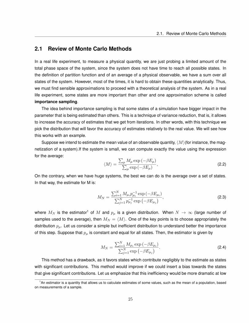
2.1 Review of Monte Carlo Methods

In a real life experiment, to measure a physical quantity, we are just probing a limited amount of the

total phase space of the system, since the system does not have time to reach all possible states. In

the definition of partition function and of an average of a physical observable, we have a sum over all

states of the system. However, most of the times, it is hard to obtain these quantities analytically. Thus,

we must find sensible approximations to proceed with a theoretical analysis of the system. As in a real

life experiment, some states are more important than other and one approximation scheme is called

importance sampling.

The idea behind importance sampling is that some states of a simulation have bigger impact in the

parameter that is being estimated than others. This is a technique of variance reduction, that is, it allows

to increase the accuracy of estimates that we get from iterations. In other words, with this technique we

pick the distribution that will favor the accuracy of estimates relatively to the real value. We will see how

this works with an example.

Suppose we intend to estimate the mean value of an observable quantity, 〈M〉(for instance, the mag-

netization of a system).If the system is small, we can compute exactly the value using the expression

for the average:

〈M〉 =

∑µMµ exp (−βEµ)∑µ exp (−βEµ)

, (2.2)

On the contrary, when we have huge systems, the best we can do is the average over a set of states.

In that way, the estimate for M is:

MN =

∑Ni=1Mµip

−1µi exp (−βEµi)∑N

j=1 p−1µj exp

(−βEµj

) , (2.3)

where MN is the estimator1 of M and pµ is a given distribution. When N → ∞ (large number of

samples used to the average), then MN = 〈M〉. One of the key points is to choose appropriately the

distribution pµ. Let us consider a simple but inefficient distribution to understand better the importance

of this step. Suppose that pµ is constant and equal for all states. Then, the estimator is given by

MN =

∑Ni=1Mµi exp (−βEµi)∑Nj=1 exp

(−βEµj

) . (2.4)

This method has a drawback, as it favors states which contribute negligibly to the estimate as states

with significant contributions. This method would improve if we could insert a bias towards the states

that give significant contributions. Let us emphasize that this inefficiency would be more dramatic at low

1An estimator is a quantity that allows us to calculate estimates of some values, such as the mean of a population, basedon measurements of a sample.

25

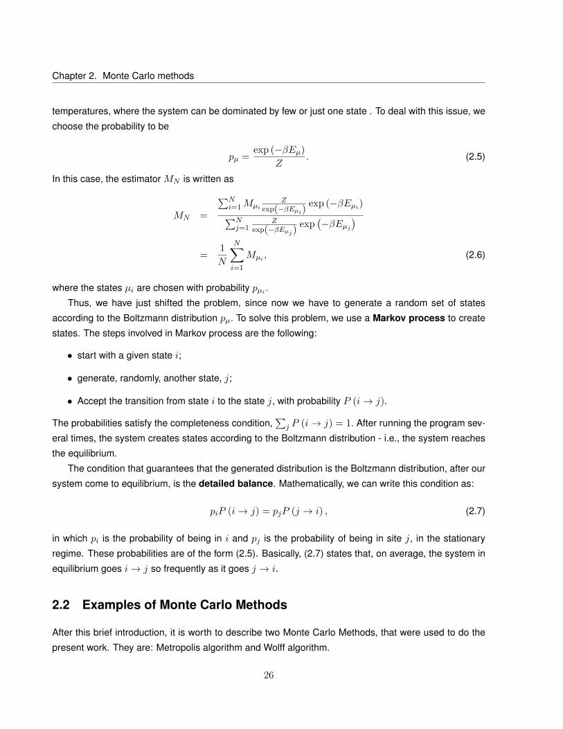
Chapter 2. Monte Carlo methods

temperatures, where the system can be dominated by few or just one state . To deal with this issue, we

choose the probability to be

pµ =exp (−βEµ)

Z. (2.5)

In this case, the estimator MN is written as

MN =

∑Ni=1Mµi

Zexp(−βEµi)

exp (−βEµi)∑Nj=1

Zexp(−βEµj )

exp(−βEµj

)=

1

N

N∑i=1

Mµi , (2.6)

where the states µi are chosen with probability pµi .

Thus, we have just shifted the problem, since now we have to generate a random set of states

according to the Boltzmann distribution pµ. To solve this problem, we use a Markov process to create

states. The steps involved in Markov process are the following:

• start with a given state i;

• generate, randomly, another state, j;

• Accept the transition from state i to the state j, with probability P (i→ j).

The probabilities satisfy the completeness condition,∑

j P (i→ j) = 1. After running the program sev-

eral times, the system creates states according to the Boltzmann distribution - i.e., the system reaches

the equilibrium.

The condition that guarantees that the generated distribution is the Boltzmann distribution, after our

system come to equilibrium, is the detailed balance. Mathematically, we can write this condition as:

piP (i→ j) = pjP (j → i) , (2.7)

in which pi is the probability of being in i and pj is the probability of being in site j, in the stationary

regime. These probabilities are of the form (2.5). Basically, (2.7) states that, on average, the system in

equilibrium goes i→ j so frequently as it goes j → i.

2.2 Examples of Monte Carlo Methods

After this brief introduction, it is worth to describe two Monte Carlo Methods, that were used to do the

present work. They are: Metropolis algorithm and Wolff algorithm.

26

2.2. Examples of Monte Carlo Methods

2.2.1 Metropolis algorithm

The Metropolis algorithm was created by Nicolas Metropolis and collaborators in 1953 [14]. The goal is

to get random samples from a certain probability distribution, for which is difficult to directly sample.

According to this method, the states are created from previous states, using the transition probability,

that depends on the difference of energies between the final and the initial states.

It is vastly used in Monte Carlo, giving, for example, the possibility of having the thermodynamic

quantities of a system of spins. Once that this work focus on Ising Model, let us describe what is the

mechanism of the method in a system of spins:

• Choose one spin, randomly, in position i;

• Calculate the difference of energy between initial configuration and the configuration with the spin

in the position i inverted: ∆E;

• Generate a random number, r (chosen uniformly in [0, 1]);

• If r < exp(− 4EkBT

), flip the spin.

Then, we choose another site, calculate again the difference between energies, generate a random

number and compare it with the Boltzmann factor, and so on, until reach every spin. This algorithm, that

allows to flip a single spin, is said to have single-spin-flip dynamics.

2.2.2 Wolff algorithm

The correlation length of the system increases in the vicinity of the critical point of a phase transition.This

induces the formation of domains - group of spins that point in the same direction. Since they have the

same orientation, there will be a strong ferromagnetic interaction between pairs and it will be more

difficult to flip every spin of the domain. The cost of inverting a spin is 2zJ , in which z is the coordination

number (number of first neighbors). If the spin is in the edge of the domain, it requires less energy to

flip. However, using a single-spin-flip algorithm to try to invert the whole domain takes a considerably

amount of time. Thus, we need a more efficient way to perform this task.

The Wolff algorithm was proposed by the man with the same name, Ulli Wolff, in 1989 [22], based

in works of Swedsen and Wang (1987) [21]. The idea is searching for clusters - i.e., sets of spins which

are correlated - and inverting all the cluster at once (and not spin by spin). Algorithms of this type are

called cluster-flipping algorithms.

This algorithm satisfies the detailed balance and the probability of adding a spin to the cluster (in

the Ising Model) is Padd = 1− exp (−2βJ) .

The recipe for Wolff algorithm is the following:

27

Chapter 2. Monte Carlo methods

• Choose a spin, randomly, from the lattice;

• Verify the neighbors. If they are pointing in the same direction, they can be added to the cluster

with probability Padd. If not, they are not added to the cluster.

• For every added spin, check out its neighbors and, if they have the same orientation, add them

with probability Padd. Notice that it is possible to have spins that we checked but they already

belong to the cluster; in this case, we will not add it again. On the other hand, we can be testing

spins that have been tested before, but were rejected with probability 1−Padd. In these conditions,

they can have now the possibility of joining the cluster. This process is repeated until every spin

is tested.

• Finally, invert the cluster.

2.3 Metropolis vs Wolff Algorithms

In spite of being more complex to implement than Metropolis algorithm, we will see that the Wolff algo-

rithm provides accurate results in the region that we are interested in: the critical region. However, Wolff

method is slower than Metropolis algorithm both at high and low temperatures.

When the temperature is very high, the spins, generally, are not aligned in the same direction. For

this reason, most of the times, the cluster is just one spin. In this way, the Wolff algorithm only inverts

one spin - and that is exactly what Metropolis algorithm does. Nevertheless, the Wollf is slower because

it will check the alignment of every neighbor spin, while Metropolis only has to decide when to flip.

If the temperature is low, Padd is very high, because almost every spins point in the same direction.

Therefore, it is probable to choose a spin and all its neighbors are aligned like it. The cluster becomes

huge and can occupy all the lattice. Consequently, the large cluster (or all lattice) is inverted only once,

after the checking of every neighbor, that costs time.

How can we know that Wolff algorithm is better in critical region? How can we quantify it? In order

to understand this, let us introduce the quantity z, called dynamic exponent.

Let us remark that the exponent z is not an universal exponent, because it depends on the algorithm

we are using to do the simulation. For temperatures near the critical temperature, the autocorrelation

time, τ , that is the time needed for the system to loose memory of the initial state2, goes with the length

of the lattice in this way:

τ ∝ Ld+z, (2.8)

2This is a poor explanation of what really is the autocorrelation time. Nevertheless, it will become clear in chapter 3.

28

2.3. Metropolis vs Wolff Algorithms

10 100 1000L

1

10

100

τcp

uτ

CPU |M|(L)

τCPU Energy

(L)

τCPU |M|

(L) = 0.62 L0.499

τCPU Energy

(L) = 0.53 L0.561

Wolff Method

10 100L

1

10

100

1000

10000

τcp

u

τCPU |M|

(L)

τCPU Energy

(L)

τCPU |M|

(L) = 0.19 L2.08

τCPU Energy

(L) = 0.19 L1.77

Metropolis Method

Figure 2.1: τCPU for absolute magnetization and for energy, depending on L, for 2D Ising Model, usingdifferent algorithms: Wolff and Metropolis. It was used the Tc of 2D Ising Model. The points are theexperimental measurements and the dotted line is a power regression of data.

where d is the dimensionality of the system. This power law dependence is very common in critical

phenomena.

A large value of z indicates that, as we approximate the critical temperature, the simulation is slower

and less accurate. On the contrary, a small z indicates a small critical slowing down and a faster

algorithm. z = 0 means that there is no critical slowing down and the corresponding algorithm can

be used until the critical temperature, without τ becoming very large. The critical slowing down is an

abnormal growth of the autocorrelation time close to the critical temperature.

Notice that we must be very careful in order to be fair to measure the autocorrelation time in Metropo-

lis and Wolff methods. For Metropolis algorithm, the computation time is the same at any temperature

and is given by:

τCPU =τ

Ld, (2.9)

i.e., is measured in Monte Carlo Steps (MCS): 1MCS ≡ Ld. It is the best choice for measure

because, to uncorrelate all spins in Metropolis algorithm, we need to run the simulation at least Ld, that

is, the size of the lattice.

In the case of Wolff algorithm, the computation time varies with temperature. Thus, in the compu-

tation of τCPU , beyond the autocorrelation time of the system, we have to take into account the time

needed to execute a step of Markov chain. This is proportional to the average number of tested spins

(for each temperature):

τCPU = τηβLd, (2.10)

29

Chapter 2. Monte Carlo methods

10 100L

10

100

1000τ

CP

Uτ

CPU |M| (L)

τCPU Energy

(L)

τCPU |M|

(L) = 0.3 L1.99

τCPU Energy

(L) =0.36 L1.79

Metropolis Algorithm

10 100L

1

10

100

1000

τCPU |M|

(L)

τCPU Energy

(L)

τCPU |M|

(L)= 0.5L1.2

τCPU Energy

(L) = 0.92L1.4

Wolff Algorithm

Figure 2.2: τCPU for absolute magnetization and for energy, depending on L, for 3D Ising Model, usingdifferent algorithms: Wolff and Metropolis. It was used the Tc of 3D Ising Model. The points are theexperimental measurements and the dotted line is a power regression of data.

in which ηβ is the number of flipped spins.

Studying the τCPU for different size systems, for 2D Ising Model, we obtained the plot of fig.(2.1). In

graph (2.1), we can observe the τCPU for the 2D Ising Model, with two different algorithms, for different

lattice sizes: 42, 82, 162, 322, 642, 1282, 2562, 5122 for Wolff algorithm and 42, 82, 162, 322, 642, 1282,

2562 for Metropolis. We performed measurements of τCPU in the calculation of absolute magnetization

and average energy of the system. In both cases, we find that z is lower for the Wolff technique, which

means that it is better than Metropolis in measuring near critical temperature. It costs less CPU time.

The time scale for the simulation is the higher autocorrelation time measured; in this case, it is τCPU Efor Wolff algorithm and τCPU |M |for Metropolis algorithm.

In the literature, we can find different measures of z, using a wide variety of methods of measure-

ment. The range of values for algorithms that flips only one spin at a time, such as the Metropolis, varies

between z = 1.7 and z = 2.7. The reference value, till the moment, for z, for these type of algorithms,

was calculated by Nightingale and Blöte in 1996 [17] , and is z = 2.1665 ± 0.0012. In the case of

zWolff , the best calculation belongs to Coddington and Baillie (1992) [7] and is zWolff = 0.25 ± 0.01.

For Metropolis algorithm, we find z = 2.08 and for Wolff zWolff = 0.561. In the plot (2.1) , for Wollf

algorithm, it is possible to note a slight curvature of the data. If we calculate the autocorrelation time for

larger systems, probably, the dynamic exponent will decrease, reaching the tabulated values, or even

30

2.3. Metropolis vs Wolff Algorithms

correct them. It was not done because it takes too much time to get z values for higher systems.

In any case, the value of z is smaller for Wolff algorithm, so, it is the best method to use near critical

temperature. Once that the present work studies the critical region, in all measurements, we use the

Wolff algorithm.

For the 3D Ising Model, in the literature, the value of z is 2.08 [15] , using the Metropolis algorithm. In

the case of using the Wolff algorithm, the value of z is 0.44 [8]. In fig.(2.2), we performed a measurement

of z using both algorithms.

We used lattices of size 43, 83, 163 and 323 for Metropolis and lattices of size 43, 83, 163, 323 and

643 for Wolff. τCPU was calculated using the estimate of critical temperature for the 3D Ising Model,

that is βC 3D = 0.2216595 [11]. We find that z = 1.99 for Metropolis algorithm and that z = 1.4 for Wolff

Algorithm.

31

Chapter 3

Averages and errors in a Markov chainMonte Carlo sample

This chapter is an introduction to error theory in Monte Carlo methods. We chose a toy model to apply

the techniques, in order to understand how we calculate the averages and errors. The interested reader

can find more information in references [1],[24].

3.1 Definitions

Assume that we have a series of data points generated by a Monte Carlo process in equilibrium:

• the probability of each event is independent of time;

• the probability of a pair of events, one at time ti and other at ti+m, only depends on the difference

of time: t = ti+m − ti.

The moments for each value of xt are given by the equilibrium probability distribution, P (x),

〈xnt 〉 = 〈xn〉 =

ˆdxxnP (x) . (3.1)

It is useful to define the covariance between two variables,

χxy = 〈xy〉 − 〈x〉 〈y〉 , (3.2)

32

3.2. Toy model of correlated data

and the cross averages involving different times,

〈xt1yt2〉 =

ˆdx

ˆdy xyP (x, t1; y, t2)

=

ˆdx

ˆdy xyP (y, t2|x, t1)P (x, t1) , (3.3)

If we are dealing with a Markov process in equilibrium:

P (x1, t1) = P (x) (3.4)

P (y, t2|x, t1) = P (y, (t2 − t1) |x, 0) , (3.5)

that is, the average 〈xt1yt2〉 only depends on the difference of time.

If the Markov process respects the detailed balance,

P (y, t2|x, t1)P (x) = P (x, t2|y, t1)P (y) , (3.6)

and we get

〈xt1yt2〉 = 〈yt1xt2〉 = 〈xy〉 (t2 − t1) . (3.7)

Other important quantity is the normalized correlation function:

Cxy (t) =〈xy〉 (t)− 〈y〉 〈x〉

χxy. (3.8)

The autocorrelation time is the sum over all instants of the correlation function:

τ =

∞∑t=1

C (t) . (3.9)

These general statements will be useful to understand the next sections.

3.2 Toy model of correlated data

The aim of a toy model is to use a simpler model to understand more complex systems. It allows us to

calculate some properties and verify them easily, so that we can know if we are in the right direction.

The chosen toy model is the one dimensional (1D) random walk “in a box”, with periodic boundary

conditions, that is described below.

Suppose that we have a 1D box of length L and periodic boundary conditions, i.e., we can identify

L ≡ 0 (see fig. (3.1)). The walker is allowed to walk a path of T steps in the box, but with some

33

Chapter 3. Averages and errors in a Markov chain Monte Carlo sample

0 1 2 L≡0L-1

01L

2L

1L - 1L

Figure 3.1: Representation of the path of the walker. Notice that we normalize the positions by thelength (L) of the “box”.

conditions: he can walk one step to the right with probability pr, one step to the left with probability pl or

stay in the same spot with probability ps. If we enable the walker to take a large number of steps, in the

end, what happens is that the probability of being in any spot in the box is the same. In other words, the

system reaches the asymptotic limit. In this case, the probability is:

p =1

L. (3.10)

Therefore, in the equilibrium, the mean value of the position in which the walker can be is given by:

〈x〉 =L−1∑k=0

k

(L− 1)p (3.11)

=

L−1∑k=0

k

(L− 1)

1

L

=1

2,

where we divided the positions by the size of the system. The mean value for x2 is:

⟨x2⟩

=L−1∑k=0

(k

(L− 1)

)p =

1

6

(2L− 1)

(L− 1). (3.12)

Thus, with (3.11) and (3.12), we can build the variance for the system in equilibrium:

⟨x2⟩− 〈x〉2 =

1

6

(2L− 1)

(L− 1)− 1

4. (3.13)

In the following sections, we will test these equations.

34

3.2. Toy model of correlated data

3.2.1 Analytical evolution in time

The goals of using this toy model are: study it in an analytical way, since it can be solved exactly; perform

simulations and compare them with the results provided by the exact solution; and, in the next sections,

use the data from simulations to illustrate some results of error theory.

For the system of the 1D random in a box with periodical boundary conditions, the master equation

that governs the temporal evolution of probability of being in a position k, Pk, (do not forget that we are

considering only the transitions between first neighbor positions) is:P0 (t+ 1) = plP1 (t) + prPL−1 (t) + (1− pr − pl)P0

Pk (t+ 1) = plPk+1 (t) + prPk−1 (t) + (1− pr − pl)Pk (t) , 0 < k < L− 1

PL−1 (t+ 1) = plP0 (t) + prPL−2 (t) + (1− pr − pl)PL−1

. (3.14)

With this system of equations, we are able to construct a matrix - the Markov matrix, Ωij . In this way,

we have a rule to relate the positions of the walker at instants t and t+ 1:

Pi (t+ 1) =∑j

ΩijPj (t) . (3.15)

This Markov matrix is of the form:

(1− pr − pl) pl 0 . . . pr

pr (1− pr − pl) . . . . . . 0

0...

. . ....

. . .

pl pr (1− pr − pl)

. (3.16)

The calculation of eigenvectors and eigenvalues of the Markov matrix will be determinative for getting

the correlation function between two points separated in time, as we will see in (3.30).

The equation for eigenvalues and eigenvectors is:

Ωijϕj = λϕj . (3.17)

To simplify, we assume that it is a diffusion process. In a diffusion process, the velocity of a given

particle is zero; however, in this particular case of study, we do not deal with velocities, but with prob-

abilities. Thus, for a diffusion process in a random walk, pr = pl. Notice that if, for instance, pr > pl,

the walker would move more often to the right than to the left. To simplify the notation, let us write

pr = pl = p.

Note that there are right eigenvectors, as in (3.17), and left eigenvectors. Generally, they are not the

35

Chapter 3. Averages and errors in a Markov chain Monte Carlo sample

same. However, in this specific case, once that Ωij is symmetric (because pr = pl ), the left and right

eigenvectors are the same.

In this way, the system (3.17) is:λϕ0 = pϕ1 + pϕN−1 + (1− 2p)ϕ0

λϕk = pϕk+1 + pϕk−1 + (1− 2p)ϕk, 0 < k < L− 1

λϕL−1 = pϕ0 + pϕL−2 + (1− 2p)ϕL−1

(3.18)

Considering the periodic boundary conditions and that the component j of ϕ, the eigenvector, is of

the form

ϕkj = exp

(i2π

Lkj

), (3.19)

we get the expression for the spectrum of eigenvalues:

λk = 1− 2p+ 2p cos

(2π

Lk

). (3.20)

Here, λk = λL+k = λ−k = λL−k and k ∈ 0, 1, ..., L− 1.Remark that it is possible to write the probability of being in position j at instant t = 0, Pj (0) , as a

linear combination of its eigenvectors:

Pj (0) =∞∑k=1

akϕkj . (3.21)

So, the challenge is now to find the ak coefficients. To do that, we have to apply the inner product:∑j

(ϕk′j

)∗Pj (0) =

∑k∈S

∑j

ak

(ϕk′j

)∗ϕkj , (3.22)

where the ∗ denotes the complex conjugate. The expression to the ak coefficients is:

ak′ =

∑j

(ϕk′j

)∗Pj (0)

L. (3.23)

Moreover, it is possible to write Ωn in this way:

Ωn = S−1DnS, (3.24)

where S−1 is the vector of transposed eigenvectors of Ω, D is a matrix of respective eigenvalues

36

3.2. Toy model of correlated data

0 20 40 60 80 100m

0

0,1

0,2

0,3

0,4

Pro

bab

ilit

yT=1T=2T=8T=32T=128T=512T=2048T=8192

Probabilities DistributionTemporal Evolution

Figure 3.2: Evolution with time for P (m, t|l, 0), with a box of L = 100 and p = 0.3, starting in l = L2 .

T is the number of steps of the walker. In this plot, we do not normalize the positions by the size of thesystem. Therefore, pequilibirum = 0.01.

and S is the vector of eigenvectors. Therefore, we achieve:

[Ωt]lm

=1

L

L−1∑k=0

exp

(i2πk (m− l)

L

)λtk. (3.25)

If we are interested in calculate the probability of being in a position m, at instant t, knowing that the

walker was in a position l at instant 0, P (m, t|l, 0), we have to do:

P (m, t|l, 0) =[Ωt]ml. (3.26)

We can observe that, when t → ∞, the probability approaches to the value given by (3.10), that is

the asymptotic limit. Once again, this happens because the case in study is diffusive. Thus, starting

from any initial position, the diffusion will spread the probability for all positions. Since there is a limited

number of positions, this process will converge in a uniform distribution.

In graph (3.2), we can observe the distribution of probabilities, evolving with time. Notice that, as

time increases, the distribution becomes more and more soft, and culminates in a uniform distribution,

as expected.

37

Chapter 3. Averages and errors in a Markov chain Monte Carlo sample

3.2.2 Autocorrelation Dynamics

Now, we will focus on the analytical study of the autocorrelation function of positions and the autocorre-

lation time for this system. The autocorrelation function of positions, C(n), is defined as the way that a

position at time t is related with itself at time t + n. The autocorrelation time, τ , is the time needed to

uncorrelate the positions at different instants of time. The mathematical expressions are, recalling (3.8)

and (3.9):

C(n) =〈x (t) x (t+ n)〉 − 〈x (t)〉 〈x (t+ n)〉

〈x2 (t)〉 − 〈x (t)〉2(3.27)

τ =∞∑n=1

C (n) . (3.28)

In order to calculate the correlation function (3.27), we should compute 〈x (t) x (t+ n)〉 (we know 〈x (t)〉and 〈x (t+ n)〉 from (3.11) and

⟨x2 (t)

⟩− 〈x (t)〉2 from (3.13)) .

First of all, the expression for 〈x (t) x (t+ n)〉 is:

〈x (t) x (t+ n)〉 =

L−1∑l=0

l

(L− 1)pl

L−1∑m=0

m

(L− 1)pm (3.29)

In this way, we are able to do:

〈x (t) x (t+ n)〉 =1

L

L−1∑l,m=0

l

(L− 1)

1

L

m

(L− 1)

L−1∑k=0

exp

(i2πk (m− l)

L

)λnk . (3.30)

For the case k = 0, we get (see in (3.20) that λ0 = 1):

1

(L− 1)2 L2

L−1∑l,m=0

lm =1

4. (3.31)

So, the expression for (3.27) is:

C(n) =

14 +

∑L−1k=1

λnksin2(πkL )

− 14

16

(2L−1)(L−1) −

14

(3.32)

=3

L2 − 1

L−1∑k=1

λnksin2

(πkL

) . (3.33)

In turn, the autocorrelation time is given by:

38

3.2. Toy model of correlated data

0 20 40 60 80 100n

1e-05

0,0001

0,001

0,01

0,1

1

C(n

)SimulatedExact

Autocorrelation FunctionL=10, p=0.3

Figure 3.3: Autocorrelation function.

τ = 3L2−1

L−1∑k=1

∞∑n=1

λnksin2

(πkL

)=

3

L2 − 1

L−1∑k=1

λk

sin2(πkL

)(1− λk)

=11 + L2 − 60p

60p. (3.34)

We can, also, compute another quantity, which we call γ, and we define by:

γ =

∞∑n=1

nC (n) (3.35)

=3

L2 − 1

L−1∑k=1

∞∑n=1

nλnksin2

(πkL

) (3.36)

=

(L2 − 1

) (27 + 2

(L2 − 1

)− 84p

)+ 72 (3− 14p)

5040p2(3.37)

For a box of L = 10 and p = 0.3, we get the fig.(3.3). In the plot (3.3), we can observe the auto-

39

Chapter 3. Averages and errors in a Markov chain Monte Carlo sample

10 100L

1

10

100

1000

10000τ

τsimulated

(L)

τ(L) = 0.056 L1.99

Dependence of τ with L

Figure 3.4: Autocorrelation time depending on the length of the box.

correlation function for the positions of walker in different instants of time. The axes are in logarithmic

scale. We can infer that the simulation generated with a computational program agrees with theoretical

prediction. For large n, the concordance is not very good, due the lack of statistic. When one integrates

this function, according to (3.34), one gets the autocorrelation time.

We can verify how autocorrelation time depends on the length of the box, in fig.(3.4).In graph (3.4)

we find that τ ∼ L2, that agrees with the analytical prediction. In fact, if we compare with (3.34), the

constant of the L2 is 160×0.3 ∼ 0, 0556. Beyond that, this is an expected result, since it is a diffusive

process.

3.3 Estimation of statistical quantities

As it was emphasized in the chapter 2, the estimators give us an accurate value of the quantity that we

are measuring, for a large sample of data.

In this section, we intend to investigate which is the best estimator for the mean value, the variance

and the kurtosis (we will introduce this quantity later, in this subsection) for the data obtained from

toy model. The other goals are to find the error in estimation of these quantities and show the more

efficient way to implement the estimator calculation in the computer program, i.e., to get the recurrence

equations for the mean value, variance and kurtosis.

40

3.3. Estimation of statistical quantities

3.3.1 Mean Value

3.3.1.1 Estimator

Let us find an estimator for the mean value, 〈xn〉. We can estimate 〈xn〉 for a sample of m points:

Xn (xn) =1

m

m∑t=1

xnt . (3.38)

Xn is the estimator for the mean value. Notice that Xn is a good estimator for the mean value, since

it converges to the correspondent mean value, independently of the correlations between the different

samples of x. If we perform the average of Xn, we obtain:

〈Xn (xn)〉 =1

m

m∑t=1

〈xnt 〉 = 〈xn〉 , (3.39)

where we used the fact that the distribution is stationary and, so, independent of t.

If we want to get the average of two different positions temporally separated, 〈xy〉 (t), we can build

the estimator and do its average:

X (xy, α) =1

m− α

m−α∑t=1

xtyt+α

〈Xn (xy, α)〉 = 〈xy〉 (t) = χxyCxy (t) + 〈x〉 〈y〉 . (3.40)

Remark that, with a time series of m points, we can average only over m − α points, due to temporal

separation.

3.3.1.2 Error of the average estimation

One way to know what is the error that we are committing in the measure of a quantity is to calculate

the average deviation between the estimator and the exact value of the quantity:⟨(Xn (m)− 〈xn〉)2

⟩, (3.41)

41

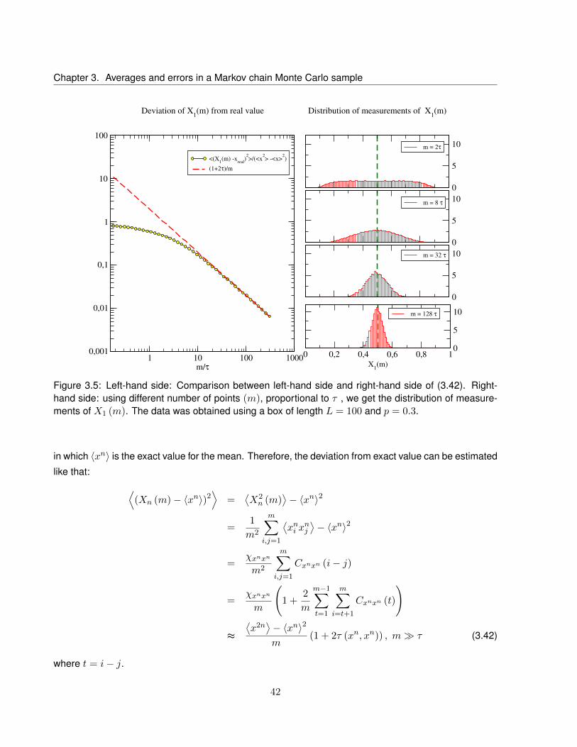
Chapter 3. Averages and errors in a Markov chain Monte Carlo sample

0

5

10m = 2τ

Distribution of measurements of X1(m)

0

5

10m = 8 τ

0

5

10m = 32 τ

0 0,2 0,4 0,6 0,8 1

X1(m)

0

5

10m = 128 τ

1 10 100 1000m/τ

0,001

0,01

0,1

1

10

100

<(X1(m) -x

real)2>/(<x

2> -<x>

2)

(1+2τ)/m

Deviation of X1(m) from real value

Figure 3.5: Left-hand side: Comparison between left-hand side and right-hand side of (3.42). Right-hand side: using different number of points (m), proportional to τ , we get the distribution of measure-ments of X1 (m). The data was obtained using a box of length L = 100 and p = 0.3.

in which 〈xn〉 is the exact value for the mean. Therefore, the deviation from exact value can be estimated

like that: ⟨(Xn (m)− 〈xn〉)2

⟩=

⟨X2n (m)

⟩− 〈xn〉2

=1

m2

m∑i,j=1

⟨xni x

nj

⟩− 〈xn〉2

=χxnxn

m2

m∑i,j=1

Cxnxn (i− j)

=χxnxn

m

(1 +

2

m

m−1∑t=1

m∑i=t+1

Cxnxn (t)

)

≈⟨x2n⟩− 〈xn〉2

m(1 + 2τ (xn, xn)) , m τ (3.42)

where t = i− j.

42

3.3. Estimation of statistical quantities

We can get a graph to compare the right-hand side and the left-hand side of (3.42) and confirm

its validity. We will use n = 1, which corresponds to 〈x〉. From the fig. (3.5), we can draw some

conclusions. On the left-hand side, when m is small, there is no coincidence between the two functions.

This is the regime where m τ , and remember that (3.42) is only valid when m τ . In fact, we

can verify that, as we increase m, the two curves get closer. On the right-hand side, we see that, as

the number of measurements increases, the value of X1 is becoming more accurate; there are more

measurements whose value is near 0.5, that is the real value for the mean value.

It is quite interesting to analyze the limits of (3.42):

• τ = 0 : this case is the standard result of m independent samples, where the error of the mean is

the standard deviation of the quantity divided by√m.

• m τ : The error still decreases with√m, because τ (xn, xn) is independent of m. Notice that

τ (xn, xn) ≈ 1

m

m−1∑t=1

m∑i=t+1

Cxnxn (t) , if m τ. (3.43)

Within this limit, we can extrapolate the limits to infinity, due to the exponential decay of the corre-

lation, and we get:

τ (xn, xn) =∞∑i=1

Cxnxn (i) , (3.44)

that is the definition of τ (see (3.9)).

• τ m 1: here, the error of the mean is basically the standard deviation of x, because the

correlation is approximately one. Averaging highly correlated measures does not decrease the

error: it is exactly the same of having only one measure.

Another nice interpretation of (3.42) is that, even if we make N averages, due to the correlations, all

the measures in groups of size 2τ + 1 are correlated. The effective number of independent samples

is m′ = m(2τ+1) or, if we have the same data and only harvesting for the mean value in a longer time

interval (2τ + 1), we will have the same error bar.

3.3.1.3 Recursion for the mean value estimator

The estimator of the mean value is given by (3.38).

The expression for m + 1 terms can be written at the expense of the m previous terms. Thus, we

43

Chapter 3. Averages and errors in a Markov chain Monte Carlo sample

reach a recurrence relation:

Xn (m+ 1) =1

m+ 1

m+1∑i=1

xni (3.45)

= Xn (m) +xnm+1 −Xn (m)

m+ 1.

This recursion prevents the loss of precision present in (3.38).

3.3.2 Variance

3.3.2.1 Estimator

The variance is given by⟨x2⟩− 〈x〉2 (it is (3.2) when x = y). For convenience, let us set σ2 = χxx, that

is the real value for the variance. We can think that a natural estimator should substitute both averages

by their estimators,

Em(σ2)

= X2 (m)−X1(m)2, (3.46)

in which Em denotes estimator. However, when one does the average of estimator (3.46), one gets:

⟨X2 (m)−X2

1 (m)⟩

=1

m

m∑i=1

⟨x2i

⟩− 〈x〉2 − χxx

m2

∑ij

Cxx (i− j)

= χxx −χxxm2

∑ij

Cxx (i− j)

= χxx

(1− 1 + 2τ (x, x)

m

). (3.47)

From (3.47), we conclude that, in fact, the best estimator is:

Em(σ2)

=m

m− 1− 2τ (x, x)

(X2 (m)−X2

1 (m)). (3.48)

Notice that the factor mm−1−2τ(x,x) tends to a constant in the limit of large m:

limm→+∞

m

m− 1− 2τ (x, x)

(X2 (m)−X2

1 (m))

= limm→+∞

(X2 (m)−X2

1 (m)). (3.49)

It is possible to build a graph to investigate the validity of (3.47). In the left-hand side of the plot (3.6), we

see that, if we increase m, the ratio between the measured variance and the exact variance approaches

to 1. For small m, the discrepancy is bigger. On the right-hand side, as the number of measurements

increase, we get an accurate value of σ2.

44

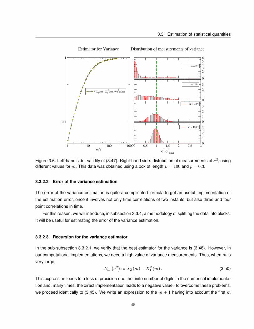
3.3. Estimation of statistical quantities

0123456

m = 2 τ

Distribution of measurements of variance

0

1

2

3m = 8τ

0

1

2

3m = 32 τ

0 0,5 1 1,5 2 2,5 3

σ2/σ

2

exact

0

1

2

3m = 128 τ

1 10 100 1000m/τ

0,5

1

< X2(m) - X

1

2(m) >/ σ

2exact

Estimator for Variance

Figure 3.6: Left-hand side: validity of (3.47). Right-hand side: distribution of measurements of σ2, usingdifferent values for m. This data was obtained using a box of length L = 100 and p = 0.3.

3.3.2.2 Error of the variance estimation

The error of the variance estimation is quite a complicated formula to get an useful implementation of

the estimation error, once it involves not only time correlations of two instants, but also three and four

point correlations in time.

For this reason, we will introduce, in subsection 3.3.4, a methodology of splitting the data into blocks.

It will be useful for estimating the error of the variance estimation.

3.3.2.3 Recursion for the variance estimator

In the sub-subsection 3.3.2.1, we verify that the best estimator for the variance is (3.48). However, in

our computational implementations, we need a high value of variance measurements. Thus, when m is

very large,

Em(σ2)≈ X2 (m)−X2

1 (m) . (3.50)

This expression leads to a loss of precision due the finite number of digits in the numerical implementa-

tion and, many times, the direct implementation leads to a negative value. To overcome these problems,

we proceed identically to (3.45). We write an expression to the m + 1 having into account the first m

45

Chapter 3. Averages and errors in a Markov chain Monte Carlo sample

terms:

σ2 (m+ 1) =m

m+ 1X2 (m) +

x2m+1

m+ 1−X2

1 (m+ 1)

=m

m+ 1σ2 (m) +

m

m+ 1X2

1 (m) +x2m+1

m+ 1−X2

1 (m+ 1)

=m

m+ 1σ2 (m)−

(X2

1 (m+ 1)−X21 (m)

)+x2m+1 −X2

1 (m)

m+ 1(3.51)

= σ2(m) +(xm+1 −X1 (m)) (xm+1 −X1 (m+ 1))− σ2 (m)

m+ 1, (3.52)

which is perfect to the calculations in the computer. Beyond that, as we will see in section 3.3.4, this

expression can be used to measure the estimator from the values of the variance inside a block of

measurements.

3.3.3 Kurtosis

The kurtosis, k, is a measure of the deviation of a distribution relatively to a Gaussian distribution (in

which k = 0), where the fourth order moments are relevant. The standard expression, for an Ising

model in zero magnetic field, is:

k =

⟨(x− 〈x〉)4

⟩⟨(x− 〈x〉)2

⟩2 − 3. (3.53)

In phase transitions, it is related with the Binder’s cumulant of the order parameter,

UB = −k3. (3.54)

The Binder’s cumulant is, frequently, used to measure Tc. When one plots the Binder’s cumulant as

function of temperature, for several system sizes, and for a given dimensionality, the curves intersect

precisely in the critical temperature [3].

3.3.3.1 Recursion relations for kurtosis

As in previous cases, it is possible to write a kurtosis recurrence relation to avoid the numerical conver-

gence problems. Thus, numerical evaluation of the kurtosis is significantly improved.

The easiest way to write the recurrence relation is to exploit the central moments, Rr. By definition,

46

3.3. Estimation of statistical quantities

the rth central moment normalized by the size of the system is given by:

Rr (L) =1

L

L−1∑i=0

(xi −X1(L))r . (3.55)

Looking this way, expression (3.53) can be rewritten as:

k (m+ 1) =R4 (m+ 1)

R22 (m+ 1)

− 3. (3.56)

The most important central moments for our calculation of the recurrence relation are:

R1 (m+ 1) = 0; (3.57)

R2 (m+ 1) = X2 (m+ 1)−X21 (m+ 1) ; (3.58)

R3 (m+ 1) = X3 (m+ 1)− 3X2 (m+ 1)X1 (m+ 1) + 2X21 (m+ 1) ; (3.59)

R4 (m+ 1) = X4 (m+ 1)− 4X3 (m+ 1)X1 (m+ 1) + 6X2 (m+ 1)X21 (m+ 1) + 5X4

1 (m+ 1) .

(3.60)

We can write R4 (m+ 1) and R3 (m+ 1) at the expense of the other central moments, always thinking

about avoiding numerical convergence problems. Note that R2 is the estimator for variance, in the limit

of large m. Doing the math, we obtain:

R2 (m+ 1) =1

m+ 1

m+1∑i=1

(xi −X1 (m+ 1))2

=m

m+ 1R2(m) +

m

(m+ 1)2 (xm+1 −X1 (m))2, (3.61)

for R3 (m+ 1):

47

Chapter 3. Averages and errors in a Markov chain Monte Carlo sample

R3 (m+ 1) =1

m+ 1

m+1∑i=1

(xi −X1 (m+ 1))3

=m

m+ 1R3 (m)− 3

m

(m+ 1)2R2 (m) (xm+1 −X1 (m))

+m (m− 1)

(m+ 1)3 (xm+1 −X1 (m))3 , (3.62)

and for R4 (m+ 1):

R4 (m+ 1) =1

m+ 1

m+1∑i=1

(xi −X1 (m+ 1))4

=m

m+ 1R4 (m)− 4R3 (m) (xm+1 −X1 (m))

m

(m+ 1)2

+ 6R2 (m) (xm+1 −X1 (m))2 m

(m+ 1)3

+ (xm+1 −X1 (m))4m(

(m+ 1)2 − 3m)

(m+ 1)4 . (3.63)

Using a box with L = 100 and p = 0.3, we calculated the distribution of the Binder’s cumulant, for dif-

ferent m. One verifies that, as one increases the number of points, the values for the Binder’s cumulant

get closer to the real value (fig. (3.7)). The analytic value for the Binder’s cumulant was found appealing

to (3.53), and it is:

Binder′s cumulant =1

3

(3−

3(−7− 7L+ 3L2 + 3L3

)5 (L− 1) (L+ 1)2

). (3.64)

In the plot of the figure (3.7), “Exact Binder” refers to the value for (3.64), when L = 100.

3.3.4 Blocks’ method

So far, we studied methods for the calculation of estimator’s errors and more efficient methods for

computational implementation of the mean value, variance and kurtosis. However, we can not forget

that there are still correlations between the data, that can introduce some errors in the estimation of the

values. In this subsection, we will study a strategy to overcome this problem.

48

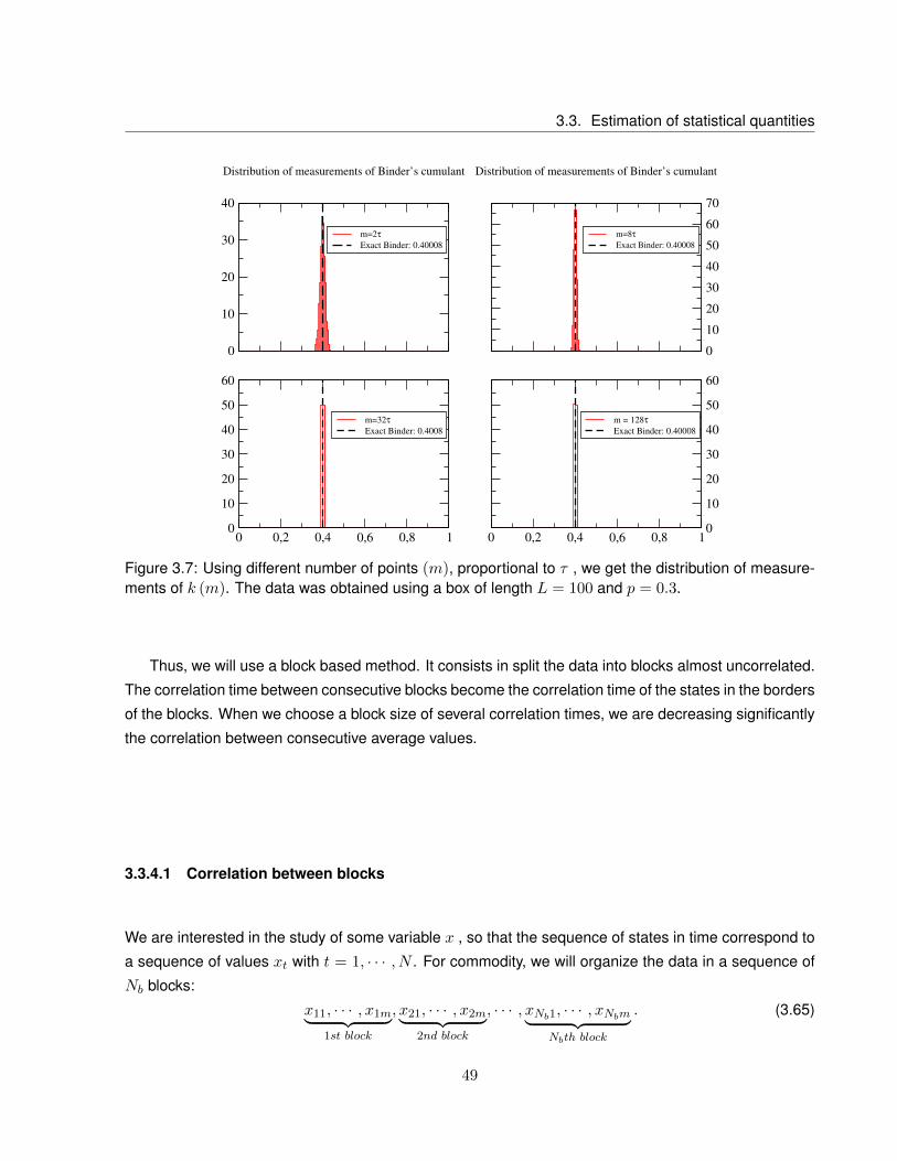
3.3. Estimation of statistical quantities

0

10

20

30

40

m=2τ

Exact Binder: 0.40008

Distribution of measurements of Binder’s cumulant

0

10

20

30

40

50

60

70

m=8τ

Exact Binder: 0.40008

Distribution of measurements of Binder’s cumulant

0 0,2 0,4 0,6 0,8 10

10

20

30

40

50

60

m=32τ

Exact Binder: 0.4008

0 0,2 0,4 0,6 0,8 10

10

20

30

40

50

60

m = 128τ

Exact Binder: 0.40008

Figure 3.7: Using different number of points (m), proportional to τ , we get the distribution of measure-ments of k (m). The data was obtained using a box of length L = 100 and p = 0.3.

Thus, we will use a block based method. It consists in split the data into blocks almost uncorrelated.

The correlation time between consecutive blocks become the correlation time of the states in the borders

of the blocks. When we choose a block size of several correlation times, we are decreasing significantly

the correlation between consecutive average values.

3.3.4.1 Correlation between blocks

We are interested in the study of some variable x , so that the sequence of states in time correspond to

a sequence of values xt with t = 1, · · · , N . For commodity, we will organize the data in a sequence of

Nb blocks:

x11, · · · , x1m︸ ︷︷ ︸1st block

, x21, · · · , x2m︸ ︷︷ ︸2nd block

, · · · , xNb1, · · · , xNbm︸ ︷︷ ︸Nbth block

. (3.65)

49

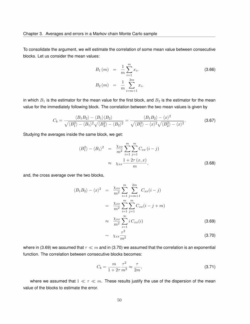
Chapter 3. Averages and errors in a Markov chain Monte Carlo sample

To consolidate the argument, we will estimate the correlation of some mean value between consecutive

blocks. Let us consider the mean values:

B1 (m) =1

m

m∑i=1

xi, (3.66)

B2 (m) =1

m

2m∑i=m+1

xi,

in which B1 is the estimator for the mean value for the first block, and B2 is the estimator for the mean

value for the immediately following block. The correlation between the two mean values is given by

Cb =〈B1B2〉 − 〈B1〉〈B2〉√

〈B21〉 − 〈B1〉2

√〈B2

2〉 − 〈B2〉2=

〈B1B2〉 − 〈x〉2√〈B2

1〉 − 〈x〉2√〈B2

2〉 − 〈x〉2. (3.67)

Studying the averages inside the same block, we get:

〈B21〉 − 〈B1〉2 =

χxxm2

m∑i=1

m∑j=1

Cxx (i− j)

≈ χxx1 + 2τ (x, x)

m, (3.68)

and, the cross average over the two blocks,

〈B1B2〉 − 〈x〉2 =χxxm2

m∑i=1

2m∑j=m+1

Cxx(i− j)

=χxxm2

m∑i=1

m∑j=1

Cxx(i− j +m)

≈ χxxm2

∞∑i=1

i Cxx(i) (3.69)

∼ χxxτ2

m2(3.70)

where in (3.69) we assumed that τ m and in (3.70) we assumed that the correlation is an exponential

function. The correlation between consecutive blocks becomes:

Cb =m

1 + 2τ

τ2

m2≈ τ

2m, (3.71)

where we assumed that 1 τ m. These results justify the use of the dispersion of the mean

value of the blocks to estimate the error.

50

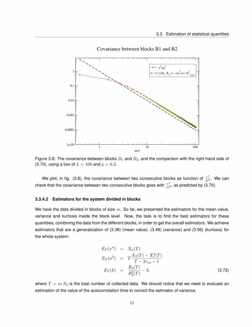
3.3. Estimation of statistical quantities

1 10 100m/τ

1e-05

0,0001

0,001

0,01

0,1

1τ

2/m

2

(<X1 X

2 > - <x

2>) / σ

2

exact

Covariance between blocks B1 and B2

Figure 3.8: The covariance between blocks B1 and B2, and the comparison with the right-hand side of(3.70), using a box of L = 100 and p = 0.3.

We plot, in fig. (3.8), the covariance between two consecutive blocks as function of τ2

m2 . We can

check that the covariance between two consecutive blocks goes with τ2

m2 , as predicted by (3.70).

3.3.4.2 Estimators for the system divided in blocks

We have the data divided in blocks of size m. So far, we presented the estimators for the mean value,

variance and kurtosis inside the block level. Now, the task is to find the best estimators for these

quantities, combining the data from the different blocks, in order to get the overall estimators. We achieve

estimators that are a generalization of (3.38) (mean value), (3.48) (variance) and (3.56) (kurtosis) for

the whole system:

ET (xn) = Xn(T )

ET (σ2) = TX2(T )−X2

1 (T )

T − 2τxx − 1

ET (k) =R4(T )

R22(T )

− 3, (3.72)

where T = mNb is the total number of collected data. We should notice that we need to evaluate an

estimation of the value of the autocorrelation time to correct the estimator of variance.

51

Chapter 3. Averages and errors in a Markov chain Monte Carlo sample

3.3.4.3 Recursion relations over blocks

Once again, until now, we just have the recursion relations to be implemented inside the block. Nev-

ertheless, to obtain the overall estimators, for the system, we need to combine the different statistical

measures from different blocks. We will present the recursion relations for the set of equations (3.72).

Let us define the estimator of the mean value, variance and kurtosis up to the l − th block:

Z1(l) = X1(ml)

Sα(l) = Rα(ml)

K(l) =S4(ml)

S22(ml)

− 3 (3.73)

For the mean value, the recursion relation is straightforward:

Z1(l + 1) = Z1(l) +zl+1 − Z1(l)

l + 1, (3.74)

because the size of each block is constant. Here, zl+1 stands for the mean value of block l + 1, i.e:

zl+1 =1

m+ 1

m(l+1)∑i=ml+1

xi (3.75)

For the variance and kurtosis, it is not so direct as the mean value. The recursion relations are [6]:

• for the variance:

S2 (l + 1) = S2 (l) +1

l + 1(s2 (l)− S2 (l)) +

l

(l + 1)2 (Z1 (l + 1)− zl+1)2 ; (3.76)

• for the 3rd moment:

S3 (l + 1) = S3 (l) +1

l + 1(s3 (l)− S3 (l))

+(Z1 (l + 1)− zl+1)3

(l + 1)3 l (l + 1)

+3 (Z1 (l + 1)− zl+1) l

(l + 1)2 (s2 (l)− S2 (l)) ; (3.77)

• for the 4thmoment:

52

3.3. Estimation of statistical quantities

S4(l + 1) = S4 (l) +1

l + 1(s4 (l)− S4 (l))

+ (Z1 (l + 1)− zl+1)4 l3 − l2 + l

(l + 1)4

+ 6 (Z1 (l + 1)− zl+1)2

(l2s2 (l) + l S2 (l)

)(l + 1)3

+4 (Z1 (l + 1)− zl+1) l

(l + 1)2 (s3 (l)− S3 (l)), (3.78)

in which sα (l) is the central moment of the block l:

sα(l) =1

m

m(l+1)∑i=ml+1

(xi − zl)α (3.79)

The computational program is more efficient when we use these recursion relations. Therefore, the

obtained data is more accurate. Nevertheless, we should remark that, even using all these methods - to

split into blocks, to use the recursion relations - it is necessary to take much longer so that we can have

statistic enough.

3.3.4.4 Error bar

The error bars are obtained from estimator for variance of a quantity, assuming that the correlation

between blocks is very small. In fact, it is possible to find some correlations between consecutive

blocks, in the edges. However, this is a small effect.

We calculate the estimator for the mean value of position, its variance and kurtosis of each block:

Q =1

l

l∑i=1

Qi, (3.80)

in which Q refers to the mean value, variance or kurtosis of each block. Thus, the squared error is given

by:

42Q =σ2Q

l

=1

l

(Q2 − Q2

) l

l − 1

=(Q2 − Q2

) 1

l − 1(3.81)

If the blocks are very large, the correlations between points inside the block are small and the error

53

Chapter 3. Averages and errors in a Markov chain Monte Carlo sample

0 200 400 600

m/τ

0,6

0,8

1

Est

imate

d E

rror/

Exact

Err

or

Simulated

Evolution of the mean’s error of block

as function of block’s size

0 100 200

m/τ

0,6

0,8

1

Evolution of the variance’s error of block

as function of block’s size

0 200 400 600

m/τ

1

2

3

4

5

Evolution of the kurtosis’ error of block

as function of block’s size

Figure 3.9: Evolution of block’s errors.

estimate is better. We can illustrate this in the following way: we simulated a large block (“an infinite

block”) and calculated its mean’s error, variance’s error and kurtosis’ error. This quantity is our exact

error of the block for its mean, variance and kurtosis. Then, we generated smaller blocks of size m and

we did the same calculations. We plotted the ratio between estimated error (it is the error from smaller

blocks) and the exact error and we get the fig. (3.9). As we can see in plot (3.9), the larger the block

size, the more accurate error we get.

3.4 Final considerations of the chapter

The results of this chapter are implemented in a computational program. Using the program, it is possi-

ble to study the critical region of 2D and 3D Ising model, which is one of the aims of this proposal. The

analysis of phase transition for those systems will be performed in the next chapter.

54

Chapter 4

Analysis of 2D and 3D Ising Model phasetransition from numerical methods

4.1 Thermodynamic functions of 2D and 3D Ising Model

In this section, we will see and discuss what happens to the thermodynamic functions for 2D and 3D

Ising Model. The βc for 2D is known exactly (it is the inverse of (1.8)) . However, we only have estimates

for the same quantity in 3D: βc 3D = 0.2216595± 0.0000026 [11]. We will show some numerical results

that allow us to find the βc.

In plot (4.1), we see the plots for 2D Ising Model. We used the technique of splitting the data in

blocks to get accurate values. Besides, we represent all the thermodynamic functions with the estimated

error bar, as was explained in chapter 3. It is interesting to notice that, for specific heat and magnetic

susceptibility, as we get closer βc, the function has a peak, instead of diverging. It is an expected result,

since we are dealing with finite systems. The peak reaches high values for larger systems.

In fig. (4.2) we plot the Binder’s cumulant. The Binder’s cumulant was introduced in the subsection

3.3.3. It is useful for determining the critical temperature, once that the curves of Binder’s cumulant will

intersect exactly in the critical temperature. This is what we see in the right-hand side of the plot (4.2).

We observe also that the smallest system (lattice with 82 spins) does not intersect in the same point

of other systems; once again, it occurs because we are dealing with finite systems. So, numerically,

from the graph (4.2), we can say that βc is in the range [0.440, 0.441], that agrees with the exact value:

βc = 12

ln(1+√

2)

∼= 0.44068679351.

For 3D Ising model, we studied 3D simple-cubic Ising model. The plots obtained are in fig. (4.3).

The plots (fig. (4.3)) for 3D model are similar to 2D case, except the critical temperature. The specific

heat and the magnetic susceptibility show a peak near the critical temperature, instead of diverging.

Again, for larger systems, the peak reaches higher values. We show plots only for three lattice sizes,

55

Chapter 4. Analysis of 2D and 3D Ising Model phase transition from numerical methods

0

0,5

1

1,5

2

2,5

3

<E

(β)>

Lattice: 8x8

Lattice: 16x16

Lattice: 32x32

Lattice: 64x64

Lattice: 128x128

0

0,2

0,4

0,6

0,8

1

|m(β

)|

Lattice: 8x8

Lattice: 16x16

Lattice: 32x32

Lattice: 64x64

Lattice: 128x128

0 0,1 0,2 0,3 0,4 0,5 0,6

β

0

0,5

1

1,5

2

2,5

3

CH

(β)

Lattice: 8x8

Lattice: 16x16

Lattice: 32x32

Lattice: 64x64

Lattice: 128x128

0 0,1 0,2 0,3 0,4 0,5 0,6

β

0

50

100

150

200

χ(β

)

Lattice: 8x8

Lattice: 16x16

Lattice: 32x32

Lattice: 64x64

Lattice: 128x128

Figure 4.1: Plots of energy, absolute magnetization, specific heat and susceptibility as function of β for2D Ising Model, using Monte Carlo Methods.

0 0,1 0,2 0,3 0,4 0,5 0,6

β

0

0,1

0,2

0,3

0,4

0,5

0,6

Bin

der

’s c

um

ula

nt

(β)

Lattice: 8x8

Lattice: 16x16

Lattice: 32x32

Lattice: 64x64

Lattice: 128x128

Binder’s cumulant for 2D Ising vs β

0,439 0,440 0,441 0,442

β

0,61

0,615

0,62

Detail of the intersection of the curves at βC

Figure 4.2: The Binder’s cumulant as function of β for 2D Ising model, using Monte Carlo Methods.

56

4.1. Thermodynamic functions of 2D and 3D Ising Model

0

1

2

3

4

<E

(β)>

Lattice: 8x8x8

Lattice: 16x16x16

Lattice: 32x32x32

0

0,2

0,4

0,6

0,8

1

|m(β

)|

Lattice: 8x8x8

Lattice: 16x16x16

Lattice: 32x32x32

0 0,1 0,2 0,3 0,4 0,5

β

0

0,5

1

1,5

2

2,5

3

CH

(β)

Lattice: 8x8x8

Lattice: 16x16x16

Lattice: 32x32x32

0 0,1 0,2 0,3 0,4 0,5

β

0

10

20

30

40

50

60

χ(β

)

Lattice: 8x8x8

Lattice: 16x16x16

Lattice: 32x32x32

Figure 4.3: Plots of energy, absolute magnetization, specific heat and susceptibility as function of β for3D Ising Model, using Monte Carlo Methods.

d 2 3

α 0 0.110(1)

β 18 0.3265(3)

γ 74 1.2372(5)

ν 1 0.6301(4)

Table 4.1: Critical exponents for 2D and 3D Ising Model. d denotes dimensionality. From: [12], [18].

because it takes longer to have accurate results for large lattices.

The Binder’s cumulant plot for 3D Ising model is in the fig.(4.4). In fig. (4.4), we used also a function

with a lattice of 643 spins. However, this function has few points, and it takes longer to get a value for

β > βc. According to the right-hand side of the plot (4.4), βc is in the range [0.220, 0.222]. It is consistent

with estimates [11] for this βc.

These plots give us a general vision of the thermodynamic functions; however, we want to study the

critical region. Namely, we want to get the critical exponents. The critical exponents for 2D Ising Model

and for 3D Ising Model are in table (1.1).

Notice that the exponents for 2D Ising Model are exact, while the critical exponents of 3D are recent

estimates [12]. In the next section, we will use finite size scaling to find the values of critical exponents.

57

Chapter 4. Analysis of 2D and 3D Ising Model phase transition from numerical methods

0 0,1 0,2 0,3 0,4 0,5

β

0

0,1

0,2

0,3

0,4

0,5

0,6

Bin

der

’s c

um

ula

nt

Lattice: 8x8x8

Lattice: 16x16x16

Lattice: 32x32x32

Lattice: 64x64x64

Binder’s cumulant for 3D Ising vs β

0,220 0,222 0,224 0,226

β

0,4

0,45

0,5

0,55

0,6

Detail of the intersection of the curves at βc

Figure 4.4: The Binder’s cumulant as function of β for 3D Ising model, using Monte Carlo Methods.

4.2 The Finite Size Scaling

As refered in the section 1.3, a finite system does not have a phase transition. This is easy to understand

from the partition function since it is a sum over finite number of regular functions, i.e., e−βEµ . The fact

that there is no phase transition can also be understood from the definition of correlation length ξ. It

defines a region of length ξ where the points are correlated. Since the system is finite, the correlation

length is also restricted to be finite. However, these effects are important only near the critical point.

We know that the correlation length becomes small when it is not near Tc. Thus, the interactions of

the degrees of freedom in this regime do not feel the finite length of the system; they behave as if

the system is infinite. Recall that Monte Carlo methods are applied to finite systems, so we need to

introduce a method to extract information from the critical region, knowing that the system has a finite

length. For this purpose, we introduce a method called finite size scaling (FSS), that allows to extract

the critical data from a finite system by studying how the physical observables vary with the length scale

L.

The idea behind this method was already used on the second chapter, where we had to determine

the dynamic exponent z, that controls how the autocorrelation time, τ , scales with the system size, at

the critical temperature. In this section, we will study how the magnetization, magnetic susceptibility and

specific heat go with temperature, for various system sizes. As was remarked, at the off-criticality the

degrees of freedom behave as if they were in infinite system. The differences will only appear near the

58

4.2. The Finite Size Scaling

critical point. Thus, the FSS will depend on how accurately the critical temperature is known. It is not

our aim obtain a sensible measure for the error made in the estimation of the critical exponents using

FSS.

Let us give an example of FSS by studying the magnetic susceptibility. The magnetic susceptibility

measures how the magnetization changes when there is an infinitesimal increment in the magnetic field,

h. In the present study, we restrict h = 0. Near the critical point, in a system with zero magnetic field,

the magnetic susceptibility behaves as

χ ∼ |t|−γ . (4.1)

FSS studies how the system changes with the system size. Thus, we should now try to rephrase (4.1)

in terms of a length scale, preferably ξ. For this purpose, note that the correlation length behaves as

ξ ∼ |t|−ν . (4.2)

Therefore, the magnetic susceptibility can be written in terms of the correlation length as

χ ∼ ξγν . (4.3)

According to what was explained above, this should depend also on the system size or, in other words,

χ = ξγν χ0

(L

ξ

), (4.4)

where χ0 is a dimensionless function, satisfying

χ0(x) =

const, x 1

0, x→ 0.(4.5)

It is more convenient to express this relation in terms of the reduced temperature, instead of the corre-

lation length ξ . This can be done by introducing another function χ that is related to χ0 by

χ (x) = x−γχ0 (xν) . (4.6)

Thus, the susceptibility can be written as

χ = Lγν χ(L

1ν t). (4.7)

Notice that, in a Monte Carlo simulation, we measure the function χ. This should be done for several

sizes of the system and for values of the temperature close to the critical point. An important remark

is that χ (x) does not depend on L, so this relation shows that there is a set of exponents γ and ν

59

Chapter 4. Analysis of 2D and 3D Ising Model phase transition from numerical methods

-10 -5 5 10t L-

1

ν

0.5

1.0

1.5

|m|Lβ/ν

82

162

322

642

1282

Figure 4.5: FSS for absolute magnetization for 2D Ising Model. t, in the x-axis, denotes reducedtemperature.

that allow to collapse all data points from several system sizes to one curve. This can be done in the

following way: rescale χ by Lνγ and express it in terms of the rescaled temperature L

1ν t; then, we should

observe that the plot χLνγ in terms of tL

1ν reduces to a single curve for all points with different L. Note

that the reduced temperature t is not known for every model. Nevertheless, we can get an estimate for

it by searching the temperature in which the susceptibility achieves it maximum.

The FSS can be applied also to the specific heat and magnetization, using an argument similar to

the described above. The FSS for that quantities give the following expressions:

c = Lαν c(L

1ν t)

(4.8)

m = L−βν m

(L

1ν t)

(4.9)

The data obtained from Monte Carlo simulations can also be collapsed into one curve, using the func-

tional dependence of the previous equations. Using Monte Carlo data, varying the value of the critical

exponents until we see the collapse of the curves, we obtained the following results:

• 2D Ising Model:

– Absolute magnetization:

The exponents involved in the FSS for the absolute magnetization are β and ν. The collapse in

fig. (4.5) was obtained with β = 0.125 and ν = 1. These results for critical exponents agree with

60

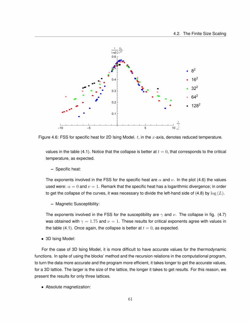
4.2. The Finite Size Scaling

-10 -5 5 10

t

L

1

ν

0.1

0.2

0.3

0.4

0.5

0.6

1

LogL

Ch

Lα/ν

82

162

322

642

1282

Figure 4.6: FSS for specific heat for 2D Ising Model. t, in the x-axis, denotes reduced temperature.

values in the table (4.1). Notice that the collapse is better at t = 0, that corresponds to the critical

temperature, as expected.

– Specific heat:

The exponents involved in the FSS for the specific heat are α and ν. In the plot (4.6) the values

used were: α = 0 and ν = 1. Remark that the specific heat has a logarithmic divergence; in order

to get the collapse of the curves, it was necessary to divide the left-hand side of (4.8) by log (L).

– Magnetic Susceptibility:

The exponents involved in the FSS for the susceptibility are γ and ν. The collapse in fig. (4.7)

was obtained with γ = 1.75 and ν = 1. These results for critical exponents agree with values in

the table (4.1). Once again, the collapse is better at t = 0, as expected.

• 3D Ising Model:

For the case of 3D Ising Model, it is more difficult to have accurate values for the thermodynamic

functions. In spite of using the blocks’ method and the recursion relations in the computational program,

to turn the data more accurate and the program more efficient, it takes longer to get the accurate values,

for a 3D lattice. The larger is the size of the lattice, the longer it takes to get results. For this reason, we

present the results for only three lattices.

• Absolute magnetization:

61

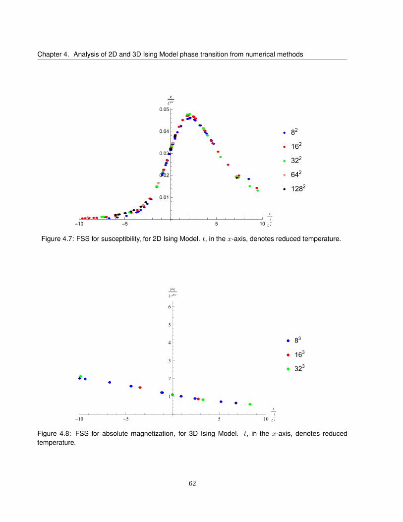
Chapter 4. Analysis of 2D and 3D Ising Model phase transition from numerical methods

-10 -5 5 10

t

L

1

ν

0.01

0.02

0.03

0.04

0.05

χ

Lγ/ν

82

162

322

642

1282

Figure 4.7: FSS for susceptibility, for 2D Ising Model. t, in the x-axis, denotes reduced temperature.

-10 -5 5 10

t

L

1

ν

1

2

3

4

5

6

m

L-β/ν

83

163

323

Figure 4.8: FSS for absolute magnetization, for 3D Ising Model. t, in the x-axis, denotes reducedtemperature.

62

4.2. The Finite Size Scaling

-10 -5 5 10

t

L

1

ν

0.2

0.4

0.6

0.8

1.0

Ch

Lα/ν

83

163

323

Figure 4.9: FSS for specific heat for 3D Ising Model. t, in the x-axis, denotes reduced temperature.

-10 -5 5 10t L-1

ν

0.01

0.02

0.03

0.04

0.05

0.06

χ L-γ/ν

83

163

323

Figure 4.10: FSS for susceptibility for 3D Ising Model. t, in the x-axis, denotes reduced temperature.

63

Chapter 4. Analysis of 2D and 3D Ising Model phase transition from numerical methods

The collapse in fig. (4.8) was obtained with β = 0.3265 and ν = 0.6301. These results for critical

exponents agree with values in the table (4.1).

– Specific heat:

The values used in fig.(4.9) were α = 0.18 and ν = 0.6301. Notice that, in 3D Ising Model, the

divergence of the specific heat is not logarithmic - α is nonzero.

– Magnetic Susceptibility:

The best collapse, that is presented in fig. (4.10), was obtained with γ = 1.2372 and ν = 0.6301.

These results for critical exponents agree with values in the table (4.1).

64

Chapter 5

Surface critical behavior results

In this section we will present the results obtained from Monte Carlo simulations for the three dimen-

sional Ising model in the presence of a spherical boundary. The procedure to simulate the Ising model

in the presence of a spherical boundary is the following: we considered a three dimensional lattice with

spins at each lattice points, drew an imaginary sphere with a certain radius in this lattice and, then, we

neglected all spins that stayed outside this region. In fig. (5.1) we give an example of this for a two

dimensional lattice.

As explained in the introduction (see subsection 1.8.5), the one and two point function of local op-

erators in the presence of a spherical boundary contain specific characteristics of conformal invariance.

We will be interested in the long wave length physics of the system, where it can be effectively viewed

as a continuum theory with local operators. The simplest local lattice operator that is invariant under the

lattice symmetries, that preserve the point x and is odd under spin-flip is the local spin field s (x). In the

sector of the operators invariant under the spin-flip and the lattice symmetries, the simplest operators

are the identity I and the energy density:

e (x) =1

6

∑δ

s (x) s (x+ δ) , (5.1)

where x + δ runs over the 6 nearest neighbors of x. The map between the lattice fields to the local

operators in the 3D Ising model assumes the following form,

s (x) = bsσa∆σσ (x) + bsσ′a

∆σ′σ′ (x) + . . .

e (x) = beII (x) + beεa∆εε (x) + beε′a

∆ε′ ε′ (x) + . . . , (5.2)

where a is the lattice spacing, ∆O is the conformal dimension of the operator. We have organized the

65

Chapter 5. Surface critical behavior results

Figure 5.1: In this example we consider a two dimensional lattice with eleven points in each side. Then,we consider a circle with radius of four lattice spacings. We count only the spins that stay inside thedisk.

local operators according to their dimension or, in other words ∆σ < ∆σ′ and ∆ε < ∆ε′ (notice that

I (x) is the identity operator, with ∆I = 0, and there is no field with dimension smaller than it). For the

3D Ising model, the best estimates for these dimensions are [9], [10] :

∆σ ≈ 0.51815, ∆σ′ ≈ 4.5, ∆ε ≈ 1.4126, ∆ε′ ≈ 3.83, (5.3)

which can be compared with the two dimensional results which are known exactly,

∆σ =1

8, ∆σ′ =

33

8, ∆ε = 1, ∆ε′ = 4. (5.4)

Log[⟨ϵ(r/R)⟩-ϵ∞]

Log[1-r2

R2]

Figure 5.2: One point function of the operator ε (x) in the presence of a spherical boundary.

66

(a) Two point function of the local operator σ (x). (b) Two point function of the local operator ε (x).

Figure 5.3: Two point function of the local operators.

The simplest one point function that is possible to compute is the local energy density ε (x), since

the one point function of the field σ (x) is zero. In fig. (5.2), we present the results for the one point

function of ε,

Notice that, for all different system sizes, the one point function of the operator ε (x) satisfies the

functional form predicted by conformal invariance. Recall that, in this case, the prediction was that the

one point function should go as a simple power law of(

1−(~rR

)2)

, as stated in (1.85). Moreover, the

exponent of the one point function is precisely the dimension of the operator ε. The conformal bootstrap

gives one of the most precise measurements of this exponent: ∆ε = 1.41267. In fig.(5.2) we have

plotted this and it clearly agrees with the data. Let us point out that the dispersion of the points for the

system with size R = 127 is large because the lack of statistics.

For the case of the two point function in the presence of a boundary, we will use both σ (x) and also

ε (x). As emphasized in the introduction, we expect that the two point function should depend just on a

non-trivial function of the conformal cross ratio ζ,

〈O∆ (~r1)O∆ (~r2)〉 =1

R24g (ζ)[(

1−(~r1R

)2)(

1−(~r2R

)2)]∆

. (5.5)

Recall we may plot the two point functions for several values of ~r1 and ~r2 that have the same cross ratio

ζ. If we obtain, for these different configurations, the same value for g (ζ) ,then, this is a strong indication

that we have indeed conformal invariance in the three dimensional Ising model. Let us just note that,

without imposing inversion symmetry, the dependence of the two point function on the arguments ~r1

67

Chapter 5. Surface critical behavior results

and ~r2 is slightly more involved.

There are two interesting limits that can be taken in the function g (ζ). They correspond to the

cases in which the two points, ~r1 and ~r2, are coming close together and the limit in which the points are

approaching the boundary. In the first case, the leading term to g (ζ) corresponds to the bulk OPE limit,

which can be predicted having information about the anomalous dimensions of the bulk operators. The

second limit corresponds to the bulk-to-boundary OPE and the leading term can be determined from

the lowest dimension boundary operators. In fig.(5.3a) and fig. (5.3b) we can check these features for

both σ (x) and ε (x) two point functions, respectively.

As can be seen for the two point function of σ ,in the limit of large ζ, the function can be well

approximated by the leading contribution from the bulk OPE. The opposite limit corresponds to the

boundary OPE and the leading contribution can be estimated using the results for the dimension of the

boundary OPE. Another property that can be seen is that the data seems to be falling on just one curve.

Recall that using conformal symmetry, different configurations of the positions ~r1 and ~r2 with the same

value of ζ should give the same result. Notice that there is a significant dispersion of the data points on

the two point function of the operator ε (x) for small value of ζ, because of lack of statistics.

68

Chapter 6

Conclusions and future work

One of the primary goals of this work was to be able to implement the known to access the critical region

of a statistical system. Along the way, we had the opportunity to understand more several subtleties that

stay outside the scope of a generic computational course. We have checked the critical Ising model

exponents and the critical temperature both for the 2D and 3D case. For this purpose, we have used

finite size scaling and other techniques, such as the Binder’s cumulant. We have also observed a strong

evidence for the conformality of the 3D Ising model. Using the results of the one and two point functions

for the critical Ising model with a spherical boundary, we were able to check dimensions of operators.

For future directions, we could try to measure three point functions in the three dimensional Ising

model and compare with the predictions coming from the conformal bootstrap approach. We could also

try to get more statistics in several simulations we have performed that would enable to reduce the error

in the estimates. We could also try to study other models that have a second phase transition and check

if they have conformal invariance.

69

Bibliography

[1] V. Ambegaokar and M. Troyer. Estimating errors reliably in Monte Carlo simulations of the Ehrenfest

model. American Journal of Physics, 78:150–157, February 2010.

[2] S. M. Bhattacharjee and A. Khare. Fifty Years of the Exact Solution of the Two-Dimensional Ising

Model by Onsager. eprint arXiv:cond-mat/9511003, November 1995.

[3] K Binder. Critical properties from monte carlo coarse graining and renormalization. Physical Re-

view Letters, 47(9):693, 1981.

[4] James J Binney, NJ Dowrick, AJ Fisher, and M Newman. The theory of critical phenomena: an

introduction to the renormalization group. Oxford University Press, Inc., 1992.

[5] John Cardy. Scaling and renormalization in statistical physics, volume 5. Cambridge University

Press, 1996.

[6] Tony F. Chan, Gene H. Golub, and Randall J. LeVeque. Algorithms for computing the sample

variance: Analysis and recommendations. The American Statistician, 37(3):pp. 242–247, 1983.

[7] Paul D Coddington and Clive F Baillie. Empirical relations between static and dynamic exponents

for ising model cluster algorithms. Physical review letters, 68(7):962, 1992.

[8] M Dilaver and M Aydin. A study of dynamic finite size scaling behavior of the scaling functions-

calculation of dynamic critical index of wolff algorithm. Technical report, 2004.

[9] Sheer El-Showk, Miguel F. Paulos, David Poland, Slava Rychkov, David Simmons-Duffin, et al.

Solving the 3D Ising Model with the Conformal Bootstrap. Phys.Rev., D86:025022, 2012.

[10] Sheer El-Showk, Miguel F. Paulos, David Poland, Slava Rychkov, David Simmons-Duffin, et al.

Solving the 3d Ising Model with the Conformal Bootstrap II. c-Minimization and Precise Critical

Exponents. J.Stat.Phys., xx:xx, 2014.

[11] Alan M. Ferrenberg and D. P. Landau. Critical behavior of the three-dimensional ising model: A

high-resolution monte carlo study. Phys. Rev. B, 44:5081–5091, Sep 1991.

70

Bibliography

[12] Hagen Kleinert. Seven loop critical exponents from strong coupling phi**4: Theory in three-

dimensions. Phys.Rev., D60:085001, 1999.

[13] David P Landau and Kurt Binder. A guide to Monte Carlo simulations in statistical physics. Cam-

bridge university press, 2009.

[14] Nicholas Metropolis, Arianna W Rosenbluth, Marshall N Rosenbluth, Augusta H Teller, and Edward

Teller. Equation of state calculations by fast computing machines. The journal of chemical physics,

21(6):1087–1092, 1953.

[15] Christian Münkel, Dieter W Heermann, Joan Adler, Misha Gofman, and Dietrich Stauffer. The

dynamical critical exponent of the two-, three-and five-dimensional kinetic ising model. Physica A:

Statistical Mechanics and its Applications, 193(3):540–552, 1993.

[16] MEJ Newman and GT Barkema. Monte carlo methods in statistical physics. 1999.

[17] MP Nightingale and HWJ Blöte. Dynamic exponent of the two-dimensional ising model and monte

carlo computation of the subdominant eigenvalue of the stochastic matrix. Physical review letters,

76(24):4548, 1996.

[18] Andrea Pelissetto and Ettore Vicari. Critical phenomena and renormalization-group theory. Physics

Reports, 368(6):549–727, 2002.

[19] Riccardo Rattazzi, Vyacheslav S. Rychkov, Erik Tonni, and Alessandro Vichi. Bounding scalar

operator dimensions in 4D CFT. JHEP, 0812:031, 2008.

[20] H Eugene Stanley. Introduction to phase transitions and critical phenomena. Introduction to Phase

Transitions and Critical Phenomena, by H Eugene Stanley, pp. 336. Foreword by H Eugene Stanley.

Oxford University Press, Jul 1987. ISBN-10: 0195053168. ISBN-13: 9780195053166, 1, 1987.

[21] Robert H Swendsen and Jian-Sheng Wang. Nonuniversal critical dynamics in monte carlo simula-

tions. Physical review letters, 58(2):86, 1987.

[22] Ulli Wolff. Collective monte carlo updating for spin systems. Physical Review Letters, 62(4):361,

1989.

[23] Julia M Yeomans. Statistical mechanics of phase transitions. Oxford University Press, 1992.

[24] Peter Young. Jackknife and bootstrap resampling methods in statistical analysis to correct for bias.

Statistical Science, 11:189–228, 1996.

71