métodos adaptativos de minería de datos y aprendizaje para ...abifet/santander.pdf · minería de...
TRANSCRIPT

Métodos Adaptativos de Minería de Datos y Aprendizajepara Flujos de Datos.
Albert Bifet
LARCA: Laboratori d’Algorismica Relacional, Complexitat i AprenentatgeDepartament de Llenguatges i Sistemes Informàtics
Universitat Politècnica de Catalunya
Junio 2009, Santander

Minería de Datos y Aprendizaje para Flujosde Datos con Cambio de Concepto
La Desintegración de laPersistencia de la Memoria
1952-54
Salvador Dalí
Extraer información de
secuencia potencialmenteinfinita de data
datos que varian con eltiempo
usando pocos recursos
usando ADWIN
ADaptive Sliding WINdow:Ventana deslizanteadaptativa
sin parámetros
2 / 29

Minería de Datos Masivos
Explosión de Datos en los últimos años
: 100 millones búsquedas por día
: 20 millones transacciones por día
1,000 millones de transacciones de tarjetas de credito por mes
3,000 millones de llamadas telefónicas diarias en EUA
30,000 millones de e-mails diarios, 1,000 millones de SMS
Tráfico de redes IP: 1,000 millones de paquetes por hora porrouter
3 / 29

Minería de Datos Masivos
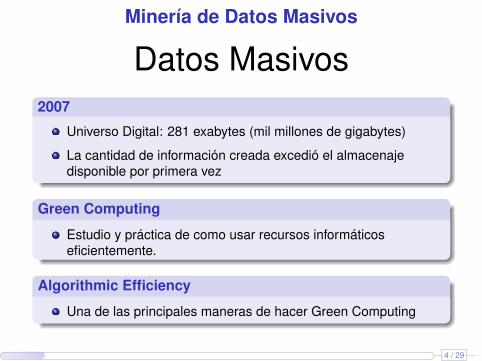
Datos Masivos2007
Universo Digital: 281 exabytes (mil millones de gigabytes)
La cantidad de información creada excedió el almacenajedisponible por primera vez
Green Computing
Estudio y práctica de como usar recursos informáticoseficientemente.
Algorithmic Efficiency
Una de las principales maneras de hacer Green Computing
4 / 29

Minería de Datos Masivos
Datos Masivos2007
Universo Digital: 281 exabytes (mil millones de gigabytes)
La cantidad de información creada excedió el almacenajedisponible por primera vez
Green Computing
Estudio y práctica de como usar recursos informáticoseficientemente.
Algorithmic Efficiency
Una de las principales maneras de hacer Green Computing
4 / 29

Minería de Datos Masivos
Koichi KawanaSimplicidad significa conseguir el máximo efecto con losmínimos medios.
Donald Knuth“... we should make use of the idea oflimited resources in our own education.We can all benefit by doing occasional"toy" programs, when artificialrestrictions are set up, so that we areforced to push our abilities to the limit. “
5 / 29

Introducción: Data Streams
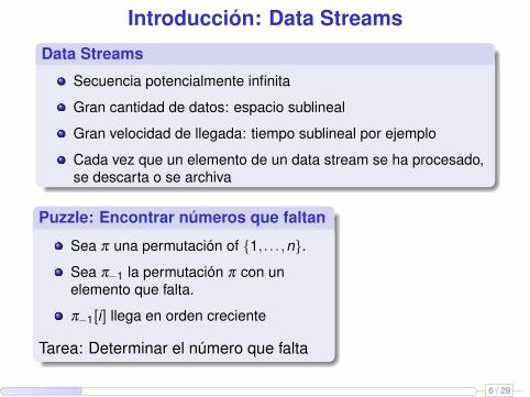
Data Streams
Secuencia potencialmente infinita
Gran cantidad de datos: espacio sublineal
Gran velocidad de llegada: tiempo sublineal por ejemplo
Cada vez que un elemento de un data stream se ha procesado,se descarta o se archiva
Puzzle: Encontrar números que faltan
Sea π una permutación of {1, . . . ,n}.
Sea π−1 la permutación π con unelemento que falta.
π−1[i] llega en orden creciente
Tarea: Determinar el número que falta
6 / 29
Introducción: Data Streams
Data Streams
Secuencia potencialmente infinita
Gran cantidad de datos: espacio sublineal
Gran velocidad de llegada: tiempo sublineal por ejemplo
Cada vez que un elemento de un data stream se ha procesado,se descarta o se archiva
Puzzle: Encontrar números que faltan
Sea π una permutación of {1, . . . ,n}.
Sea π−1 la permutación π con unelemento que falta.
π−1[i] llega en orden creciente
Tarea: Determinar el número que falta
6 / 29

Introducción: Data Streams
Data Streams
Secuencia potencialmente infinita
Gran cantidad de datos: espacio sublineal
Gran velocidad de llegada: tiempo sublineal por ejemplo
Cada vez que un elemento de un data stream se ha procesado,se descarta o se archiva
Puzzle: Encontrar números que faltan
Sea π una permutación of {1, . . . ,n}.
Sea π−1 la permutación π con unelemento que falta.
π−1[i] llega en orden creciente
Tarea: Determinar el número que falta
Usar un vectorn-bit paramemorizar todoslos numeros(espacio O(n) )
6 / 29

Introducción: Data Streams
Data Streams
Secuencia potencialmente infinita
Gran cantidad de datos: espacio sublineal
Gran velocidad de llegada: tiempo sublineal por ejemplo
Cada vez que un elemento de un data stream se ha procesado,se descarta o se archiva
Puzzle: Encontrar números que faltan
Sea π una permutación of {1, . . . ,n}.
Sea π−1 la permutación π con unelemento que falta.
π−1[i] llega en orden creciente
Tarea: Determinar el número que falta
Data Streams:espacioO(log(n)).
6 / 29

Introducción: Data Streams
Data Streams
Secuencia potencialmente infinita
Gran cantidad de datos: espacio sublineal
Gran velocidad de llegada: tiempo sublineal por ejemplo
Cada vez que un elemento de un data stream se ha procesado,se descarta o se archiva
Puzzle: Encontrar números que faltan
Sea π una permutación of {1, . . . ,n}.
Sea π−1 la permutación π con unelemento que falta.
π−1[i] llega en orden creciente
Tarea: Determinar el número que falta
Almacenar
n(n +1)
2−∑
j≤iπ−1[j].
6 / 29
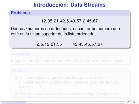
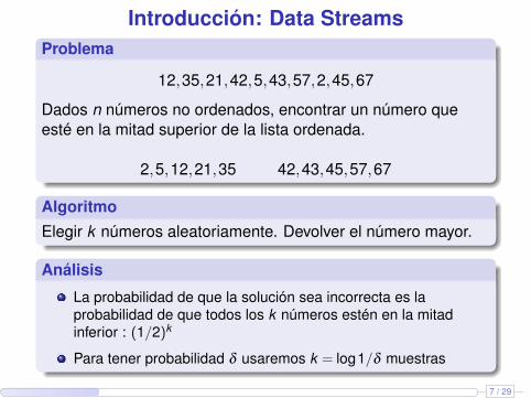
Introducción: Data StreamsProblema
12,35,21,42,5,43,57,2,45,67
Dados n números no ordenados, encontrar un número queesté en la mitad superior de la lista ordenada.
2,5,12,21,35 42,43,45,57,67
AlgoritmoElegir k números aleatoriamente. Devolver el número mayor.
Análisis
La probabilidad de que la solución sea incorrecta es laprobabilidad de que todos los k números estén en la mitadinferior : (1/2)k
Para tener probabilidad δ usaremos k = log1/δ muestras
7 / 29

Outline
1 Introduction
2 ADWIN : Concept Drift Mining
3 Hoeffding Adaptive Tree
4 Conclusions
8 / 29

Data Streams
Data StreamsAt any time t in the data stream, we would like the per-itemprocessing time and storage to be simultaneouslyO(logk (N, t)).
Approximation algorithms
Small error rate with high probability
An algorithm (ε,δ )−approximates F if it outputs F̃ for whichPr[|F̃ −F |> εF ] < δ .
9 / 29

Data Streams Approximation Algorithms
Frequency momentsFrequency moments of a stream A = {a1, . . . ,aN}:
Fk =v
∑i=1
f ki
where fi is the frequency of i in the sequence, and k ≥ 0
F0: number of distinct elements on the sequence
F1: length of the sequence
F2: self-join size, the repeat rate, or as Gini’s index ofhomogeneity
Sketches can approximate F0,F1,F2 in O(logv + logN) space.
Noga Alon, Yossi Matias, and Mario Szegedy.The space complexity of approximationthe frequency moments. 1996
10 / 29

Data Streams Approximation Algorithms
1011000111 1010101
Sliding WindowWe can maintain simple statistics over sliding windows, usingO(1
εlog2 N) space, where
N is the length of the sliding window
ε is the accuracy parameter
M. Datar, A. Gionis, P. Indyk, and R. Motwani.Maintaining stream statistics over sliding windows. 2002
11 / 29
Data Streams Approximation Algorithms
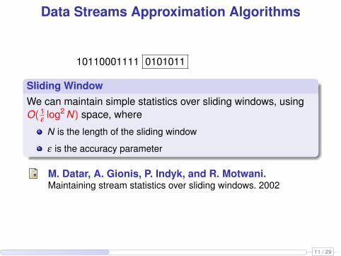
10110001111 0101011
Sliding WindowWe can maintain simple statistics over sliding windows, usingO(1
εlog2 N) space, where
N is the length of the sliding window
ε is the accuracy parameter
M. Datar, A. Gionis, P. Indyk, and R. Motwani.Maintaining stream statistics over sliding windows. 2002
11 / 29

Data Streams Approximation Algorithms
101100011110 1010111
Sliding WindowWe can maintain simple statistics over sliding windows, usingO(1
εlog2 N) space, where
N is the length of the sliding window
ε is the accuracy parameter
M. Datar, A. Gionis, P. Indyk, and R. Motwani.Maintaining stream statistics over sliding windows. 2002
11 / 29

Data Streams Approximation Algorithms
1011000111101 0101110
Sliding WindowWe can maintain simple statistics over sliding windows, usingO(1
εlog2 N) space, where
N is the length of the sliding window
ε is the accuracy parameter
M. Datar, A. Gionis, P. Indyk, and R. Motwani.Maintaining stream statistics over sliding windows. 2002
11 / 29

Data Streams Approximation Algorithms
10110001111010 1011101
Sliding WindowWe can maintain simple statistics over sliding windows, usingO(1
εlog2 N) space, where
N is the length of the sliding window
ε is the accuracy parameter
M. Datar, A. Gionis, P. Indyk, and R. Motwani.Maintaining stream statistics over sliding windows. 2002
11 / 29

Data Streams Approximation Algorithms
101100011110101 0111010
Sliding WindowWe can maintain simple statistics over sliding windows, usingO(1
εlog2 N) space, where
N is the length of the sliding window
ε is the accuracy parameter
M. Datar, A. Gionis, P. Indyk, and R. Motwani.Maintaining stream statistics over sliding windows. 2002
11 / 29
Outline
1 Introduction
2 ADWIN : Concept Drift Mining
3 Hoeffding Adaptive Tree
4 Conclusions
12 / 29

Data Mining Algorithms with Concept Drift
No Concept Drift
-input output
DM Algorithm
-
Counter1
Counter2
Counter3
Counter4
Counter5
Concept Drift
-input output
DM Algorithm
Static Model
-
Change Detect.-
6
�
13 / 29

Data Mining Algorithms with Concept Drift
No Concept Drift
-input output
DM Algorithm
-
Counter1
Counter2
Counter3
Counter4
Counter5
Concept Drift
-input output
DM Algorithm
-
Estimator1
Estimator2
Estimator3
Estimator4
Estimator5
13 / 29
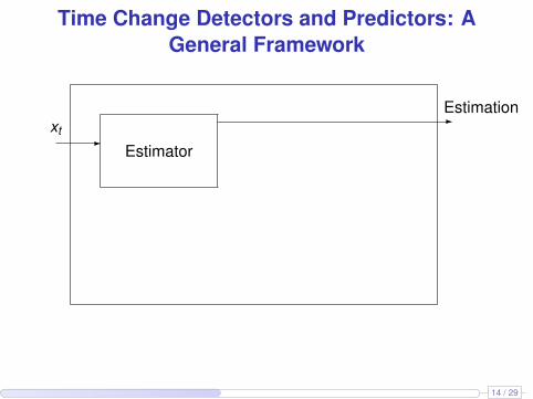
Time Change Detectors and Predictors: AGeneral Framework
-xt
Estimator
-Estimation
14 / 29
Time Change Detectors and Predictors: AGeneral Framework
-xt
Estimator
-Estimation
- -Alarm
Change Detect.
14 / 29

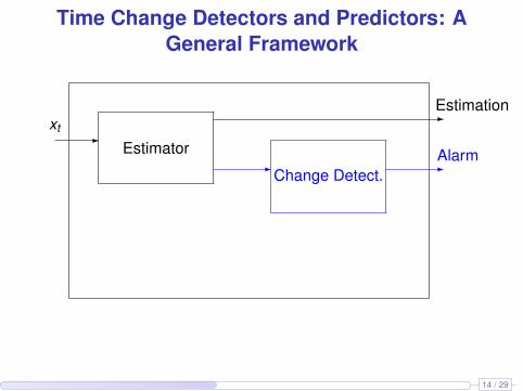
Time Change Detectors and Predictors: AGeneral Framework
-xt
Estimator
-Estimation
- -Alarm
Change Detect.
Memory-
6
6?
14 / 29

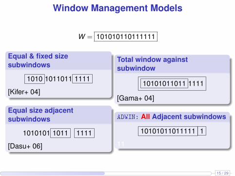
Window Management Models
W = 101010110111111
Equal & fixed sizesubwindows
1010 1011011 1111
[Kifer+ 04]
Equal size adjacentsubwindows
1010101 1011 1111
[Dasu+ 06]
Total window againstsubwindow
10101011011 1111
[Gama+ 04]
ADWIN: All Adjacent subwindows
1 01010110111111
15 / 29

Window Management Models
W = 101010110111111
Equal & fixed sizesubwindows
1010 1011011 1111
[Kifer+ 04]
Equal size adjacentsubwindows
1010101 1011 1111
[Dasu+ 06]
Total window againstsubwindow
10101011011 1111
[Gama+ 04]
ADWIN: All Adjacent subwindows
10 1010110111111
15 / 29

Window Management Models
W = 101010110111111
Equal & fixed sizesubwindows
1010 1011011 1111
[Kifer+ 04]
Equal size adjacentsubwindows
1010101 1011 1111
[Dasu+ 06]
Total window againstsubwindow
10101011011 1111
[Gama+ 04]
ADWIN: All Adjacent subwindows
101 010110111111
15 / 29

Window Management Models
W = 101010110111111
Equal & fixed sizesubwindows
1010 1011011 1111
[Kifer+ 04]
Equal size adjacentsubwindows
1010101 1011 1111
[Dasu+ 06]
Total window againstsubwindow
10101011011 1111
[Gama+ 04]
ADWIN: All Adjacent subwindows
1010 10110111111
15 / 29

Window Management Models
W = 101010110111111
Equal & fixed sizesubwindows
1010 1011011 1111
[Kifer+ 04]
Equal size adjacentsubwindows
1010101 1011 1111
[Dasu+ 06]
Total window againstsubwindow
10101011011 1111
[Gama+ 04]
ADWIN: All Adjacent subwindows
10101 0110111111
15 / 29

Window Management Models
W = 101010110111111
Equal & fixed sizesubwindows
1010 1011011 1111
[Kifer+ 04]
Equal size adjacentsubwindows
1010101 1011 1111
[Dasu+ 06]
Total window againstsubwindow
10101011011 1111
[Gama+ 04]
ADWIN: All Adjacent subwindows
101010 110111111
15 / 29

Window Management Models
W = 101010110111111
Equal & fixed sizesubwindows
1010 1011011 1111
[Kifer+ 04]
Equal size adjacentsubwindows
1010101 1011 1111
[Dasu+ 06]
Total window againstsubwindow
10101011011 1111
[Gama+ 04]
ADWIN: All Adjacent subwindows
1010101 10111111
15 / 29

Window Management Models
W = 101010110111111
Equal & fixed sizesubwindows
1010 1011011 1111
[Kifer+ 04]
Equal size adjacentsubwindows
1010101 1011 1111
[Dasu+ 06]
Total window againstsubwindow
10101011011 1111
[Gama+ 04]
ADWIN: All Adjacent subwindows
10101011 0111111
15 / 29

Window Management Models
W = 101010110111111
Equal & fixed sizesubwindows
1010 1011011 1111
[Kifer+ 04]
Equal size adjacentsubwindows
1010101 1011 1111
[Dasu+ 06]
Total window againstsubwindow
10101011011 1111
[Gama+ 04]
ADWIN: All Adjacent subwindows
101010110 111111
15 / 29

Window Management Models
W = 101010110111111
Equal & fixed sizesubwindows
1010 1011011 1111
[Kifer+ 04]
Equal size adjacentsubwindows
1010101 1011 1111
[Dasu+ 06]
Total window againstsubwindow
10101011011 1111
[Gama+ 04]
ADWIN: All Adjacent subwindows
1010101101 11111
15 / 29

Window Management Models
W = 101010110111111
Equal & fixed sizesubwindows
1010 1011011 1111
[Kifer+ 04]
Equal size adjacentsubwindows
1010101 1011 1111
[Dasu+ 06]
Total window againstsubwindow
10101011011 1111
[Gama+ 04]
ADWIN: All Adjacent subwindows
10101011011 1111
15 / 29

Window Management Models
W = 101010110111111
Equal & fixed sizesubwindows
1010 1011011 1111
[Kifer+ 04]
Equal size adjacentsubwindows
1010101 1011 1111
[Dasu+ 06]
Total window againstsubwindow
10101011011 1111
[Gama+ 04]
ADWIN: All Adjacent subwindows
101010110111 111
15 / 29

Window Management Models
W = 101010110111111
Equal & fixed sizesubwindows
1010 1011011 1111
[Kifer+ 04]
Equal size adjacentsubwindows
1010101 1011 1111
[Dasu+ 06]
Total window againstsubwindow
10101011011 1111
[Gama+ 04]
ADWIN: All Adjacent subwindows
1010101101111 11
15 / 29
Window Management Models
W = 101010110111111
Equal & fixed sizesubwindows
1010 1011011 1111
[Kifer+ 04]
Equal size adjacentsubwindows
1010101 1011 1111
[Dasu+ 06]
Total window againstsubwindow
10101011011 1111
[Gama+ 04]
ADWIN: All Adjacent subwindows
10101011011111 1
11
15 / 29

Algorithm ADWIN
Example
W= 101010110111111W0= 1
ADWIN: ADAPTIVE WINDOWING ALGORITHM
1 Initialize Window W2 for each t > 03 do W ←W ∪{xt} (i.e., add xt to the head of W )4 repeat Drop elements from the tail of W5 until |µ̂W0− µ̂W1 | ≥ εc holds6 for every split of W into W = W0 ·W17 Output µ̂W
16 / 29

Algorithm ADWIN
Example
W= 101010110111111W0= 1 W1 = 01010110111111
ADWIN: ADAPTIVE WINDOWING ALGORITHM
1 Initialize Window W2 for each t > 03 do W ←W ∪{xt} (i.e., add xt to the head of W )4 repeat Drop elements from the tail of W5 until |µ̂W0− µ̂W1 | ≥ εc holds6 for every split of W into W = W0 ·W17 Output µ̂W
16 / 29

Algorithm ADWIN
Example
W= 101010110111111W0= 10 W1 = 1010110111111
ADWIN: ADAPTIVE WINDOWING ALGORITHM
1 Initialize Window W2 for each t > 03 do W ←W ∪{xt} (i.e., add xt to the head of W )4 repeat Drop elements from the tail of W5 until |µ̂W0− µ̂W1 | ≥ εc holds6 for every split of W into W = W0 ·W17 Output µ̂W
16 / 29

Algorithm ADWIN
Example
W= 101010110111111W0= 101 W1 = 010110111111
ADWIN: ADAPTIVE WINDOWING ALGORITHM
1 Initialize Window W2 for each t > 03 do W ←W ∪{xt} (i.e., add xt to the head of W )4 repeat Drop elements from the tail of W5 until |µ̂W0− µ̂W1 | ≥ εc holds6 for every split of W into W = W0 ·W17 Output µ̂W
16 / 29

Algorithm ADWIN
Example
W= 101010110111111W0= 1010 W1 = 10110111111
ADWIN: ADAPTIVE WINDOWING ALGORITHM
1 Initialize Window W2 for each t > 03 do W ←W ∪{xt} (i.e., add xt to the head of W )4 repeat Drop elements from the tail of W5 until |µ̂W0− µ̂W1 | ≥ εc holds6 for every split of W into W = W0 ·W17 Output µ̂W
16 / 29

Algorithm ADWIN
Example
W= 101010110111111W0= 10101 W1 = 0110111111
ADWIN: ADAPTIVE WINDOWING ALGORITHM
1 Initialize Window W2 for each t > 03 do W ←W ∪{xt} (i.e., add xt to the head of W )4 repeat Drop elements from the tail of W5 until |µ̂W0− µ̂W1 | ≥ εc holds6 for every split of W into W = W0 ·W17 Output µ̂W
16 / 29

Algorithm ADWIN
Example
W= 101010110111111W0= 101010 W1 = 110111111
ADWIN: ADAPTIVE WINDOWING ALGORITHM
1 Initialize Window W2 for each t > 03 do W ←W ∪{xt} (i.e., add xt to the head of W )4 repeat Drop elements from the tail of W5 until |µ̂W0− µ̂W1 | ≥ εc holds6 for every split of W into W = W0 ·W17 Output µ̂W
16 / 29

Algorithm ADWIN
Example
W= 101010110111111W0= 1010101 W1 = 10111111
ADWIN: ADAPTIVE WINDOWING ALGORITHM
1 Initialize Window W2 for each t > 03 do W ←W ∪{xt} (i.e., add xt to the head of W )4 repeat Drop elements from the tail of W5 until |µ̂W0− µ̂W1 | ≥ εc holds6 for every split of W into W = W0 ·W17 Output µ̂W
16 / 29

Algorithm ADWIN
Example
W= 101010110111111W0= 10101011 W1 = 0111111
ADWIN: ADAPTIVE WINDOWING ALGORITHM
1 Initialize Window W2 for each t > 03 do W ←W ∪{xt} (i.e., add xt to the head of W )4 repeat Drop elements from the tail of W5 until |µ̂W0− µ̂W1 | ≥ εc holds6 for every split of W into W = W0 ·W17 Output µ̂W
16 / 29

Algorithm ADWIN
Example
W= 101010110111111 |µ̂W0− µ̂W1 | ≥ εc : CHANGE DET.!
W0= 101010110 W1 = 111111
ADWIN: ADAPTIVE WINDOWING ALGORITHM
1 Initialize Window W2 for each t > 03 do W ←W ∪{xt} (i.e., add xt to the head of W )4 repeat Drop elements from the tail of W5 until |µ̂W0− µ̂W1 | ≥ εc holds6 for every split of W into W = W0 ·W17 Output µ̂W
16 / 29

Algorithm ADWIN
Example
W= 101010110111111 Drop elements from the tail of WW0= 101010110 W1 = 111111
ADWIN: ADAPTIVE WINDOWING ALGORITHM
1 Initialize Window W2 for each t > 03 do W ←W ∪{xt} (i.e., add xt to the head of W )4 repeat Drop elements from the tail of W5 until |µ̂W0− µ̂W1 | ≥ εc holds6 for every split of W into W = W0 ·W17 Output µ̂W
16 / 29

Algorithm ADWIN
Example
W= 01010110111111 Drop elements from the tail of WW0= 101010110 W1 = 111111
ADWIN: ADAPTIVE WINDOWING ALGORITHM
1 Initialize Window W2 for each t > 03 do W ←W ∪{xt} (i.e., add xt to the head of W )4 repeat Drop elements from the tail of W5 until |µ̂W0− µ̂W1 | ≥ εc holds6 for every split of W into W = W0 ·W17 Output µ̂W
16 / 29

Algorithm ADWIN [BG07]
ADWIN has rigorous guarantees (theorems)
On ratio of false positives
On ratio of false negatives
On the relation of the size of the current window and changerates
Other methods in the literature: [Gama+ 04], [Widmer+ 96],[Last 02] don’t provide rigorous guarantees.
17 / 29

Algorithm ADWIN [BG07]
TheoremAt every time step we have:
1 (Few false positives guarantee) If µt remains constant within W,the probability that ADWIN shrinks the window at this step is atmost δ .
2 (Few false negatives guarantee) If for any partition W in twoparts W0W1 (where W1 contains the most recent items) we have|µW0 −µW1 |> ε, and if
ε ≥ 4 ·
√3max{µW0 ,µW1}
min{n0,n1}ln
4nδ
then with probability 1−δ ADWIN shrinks W to W1, or shorter.
18 / 29

Outline
1 Introduction
2 ADWIN : Concept Drift Mining
3 Hoeffding Adaptive Tree
4 Conclusions
19 / 29

Classification
Data set thatdescribes e-mailfeatures fordeciding if it isspam.
Example
Contains Domain Has Time“Money” type attach. received spam
yes com yes night yesyes edu no night yesno com yes night yesno edu no day nono com no day noyes cat no day yes
Assume we have to classify the following new instance:Contains Domain Has Time“Money” type attach. received spam
yes edu yes day ?
20 / 29

Classification
Assume we have to classify the following new instance:Contains Domain Has Time“Money” type attach. received spam
yes edu yes day ?
20 / 29
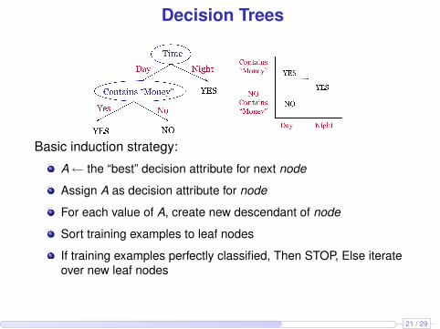
Decision Trees
Basic induction strategy:
A← the “best” decision attribute for next node
Assign A as decision attribute for node
For each value of A, create new descendant of node
Sort training examples to leaf nodes
If training examples perfectly classified, Then STOP, Else iterateover new leaf nodes
21 / 29
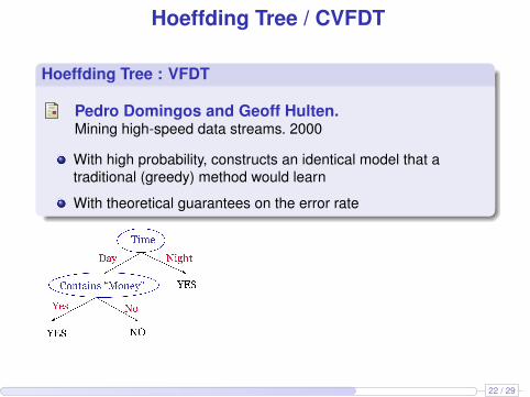
Hoeffding Tree / CVFDT
Hoeffding Tree : VFDT
Pedro Domingos and Geoff Hulten.Mining high-speed data streams. 2000
With high probability, constructs an identical model that atraditional (greedy) method would learn
With theoretical guarantees on the error rate
22 / 29

VFDT / CVFDT
Concept-adapting Very Fast Decision Trees: CVFDT
G. Hulten, L. Spencer, and P. Domingos.Mining time-changing data streams. 2001
It keeps its model consistent with a sliding window of examples
Construct “alternative branches” as preparation for changes
If the alternative branch becomes more accurate, switch of treebranches occurs
23 / 29

Decision Trees: CVFDT
No theoretical guarantees on the error rate of CVFDT
CVFDT parameters :
1 W : is the example window size.
2 T0: number of examples used to check at each node if thesplitting attribute is still the best.
3 T1: number of examples used to build the alternate tree.
4 T2: number of examples used to test the accuracy of thealternate tree.
24 / 29
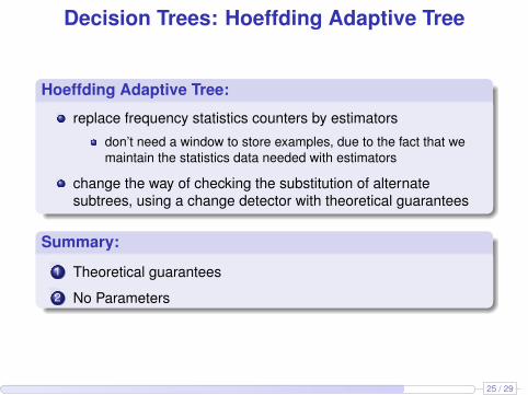
Decision Trees: Hoeffding Adaptive Tree
Hoeffding Adaptive Tree:
replace frequency statistics counters by estimators
don’t need a window to store examples, due to the fact that wemaintain the statistics data needed with estimators
change the way of checking the substitution of alternatesubtrees, using a change detector with theoretical guarantees
Summary:
1 Theoretical guarantees
2 No Parameters
25 / 29

What is MOA?
{M}assive {O}nline {A}nalysis is a framework for online learningfrom data streams.
It is closely related to WEKA
It includes a collection of offline and online as well as tools forevaluation:
boosting and baggingHoeffding Trees
with and without Naïve Bayes classifiers at the leaves.
26 / 29

Ensemble Methods
http://www.cs.waikato.ac.nz/∼abifet/MOA/
New ensemble methods:
ADWIN bagging: When a change is detected, the worst classifieris removed and a new classifier is added.
Adaptive-Size Hoeffding Tree bagging
27 / 29

Outline
1 Introduction
2 ADWIN : Concept Drift Mining
3 Hoeffding Adaptive Tree
4 Conclusions
28 / 29

Conclusions
Adaptive and parameter-free methods based in
replace frequency statistics counters by ADWIN
don’t need a window to store examples, due to the fact that wemaintain the statistics data needed with ADWINs
using ADWIN as change detector with theoretical guarantees,
Summary:
1 Theoretical guarantees
2 No parameters needed
3 Higher accuracy
4 Less space needed
29 / 29