medida y modelización de la componente difusa de la...

Universidad de Extremadura

TESIS DOCTORAL

Medida y modelizacion de lacomponente difusa de la radiacion

solar total y ultravioleta

Guadalupe Sanchez Hernandez

Departamento de Fısica

2017

Universidad de Extremadura

TESIS DOCTORAL

MEDIDA Y MODELIZACION DE LACOMPONETE DIFUSA DE LA

RADIACION SOLAR TOTAL Y UV

Guadalupe Sanchez Hernandez

DEPARTAMENTO DE FISICA

Conformidad del Director:

Fdo: Antonio Serrano Perez

2017

A mis padres

Indice general

Resumen 3

Summary 6

1. Informacion general sobre la Tesis Doctoral 7

1.1. Justificacion y coherencia unitaria de la Tesis Doctoral . . . . . . . . 7

1.2. Objetivo . . . . . . . . . . . . . . . . . . . . . . . . . . . . . . . . . . 8

1.3. Estructura de la memoria . . . . . . . . . . . . . . . . . . . . . . . . 9

2. Introduccion 11

2.1. Origen y caracterısticas de la radiacion solar difusa . . . . . . . . . . 11

2.2. Aplicaciones . . . . . . . . . . . . . . . . . . . . . . . . . . . . . . . . 14

2.2.1. Energıa solar . . . . . . . . . . . . . . . . . . . . . . . . . . . 14

2.2.2. Arquitectura solar . . . . . . . . . . . . . . . . . . . . . . . . 15

2.2.3. Salud . . . . . . . . . . . . . . . . . . . . . . . . . . . . . . . 16

2.3. Radiacion solar difusa en el marco del cambio climatico actual . . . 17

2.4. Medida de la radiacion solar difusa . . . . . . . . . . . . . . . . . . . 19

2.4.1. Radiometros de banda ancha para la media de irradiancia di-

fusa total y ultravioleta . . . . . . . . . . . . . . . . . . . . . 19

2.4.2. Dispositivos para el bloqueo de la radiacion solar directa. . . 21

2.4.3. Precision en las medidas de irradiancia difusa total y UV . . 23

2.5. Modelizacion de la radiacion solar difusa . . . . . . . . . . . . . . . . 24

Bibliografıa . . . . . . . . . . . . . . . . . . . . . . . . . . . . . . . . . . . 26

3. Error asociado al cero termico o “thermal offset” 33

3.1. Introduccion . . . . . . . . . . . . . . . . . . . . . . . . . . . . . . . . 33

3.2. Artıculo 1 . . . . . . . . . . . . . . . . . . . . . . . . . . . . . . . . . 37

3.2.1. Datos del artıculo . . . . . . . . . . . . . . . . . . . . . . . . 37

3.2.2. Principales aportaciones del artıculo . . . . . . . . . . . . . . 37

3.2.3. Copia original del artıculo . . . . . . . . . . . . . . . . . . . . 39

5

6 INDICE GENERAL

3.2.4. Informe del Director de la Tesis Doctoral . . . . . . . . . . . 53

3.3. Artıculo 2 . . . . . . . . . . . . . . . . . . . . . . . . . . . . . . . . . 54





3.4. Artıculo 3 . . . . . . . . . . . . . . . . . . . . . . . . . . . . . . . . . 70





3.5. Artıculo 4 . . . . . . . . . . . . . . . . . . . . . . . . . . . . . . . . . 86





4. Correccion del error introducido por el anillo de sombra 127

4.1. Introduccion . . . . . . . . . . . . . . . . . . . . . . . . . . . . . . . . 127

4.2. Artıculo 5 . . . . . . . . . . . . . . . . . . . . . . . . . . . . . . . . . 130



4.2.3. Copia original de artıculo . . . . . . . . . . . . . . . . . . . . 132


4.3. Artıculo 6 . . . . . . . . . . . . . . . . . . . . . . . . . . . . . . . . . 142



4.3.3. Copia original de artıculo . . . . . . . . . . . . . . . . . . . . 144


5. Modelos empıricos para la estimacion de irradiacia difusa 157

5.1. Introduccion . . . . . . . . . . . . . . . . . . . . . . . . . . . . . . . . 157

5.2. Artıculo 7 . . . . . . . . . . . . . . . . . . . . . . . . . . . . . . . . . 159





6. Principales resultados y conclusiones 187

INDICE GENERAL 7

Summary of results and main conclusions 190

8 INDICE GENERAL

Indice de figuras

2.1. Irradiancia solar espectral en el tope de la atmosfera y componentes

global, directa y difusa en la superficie terrestre resultantes de los

procesos de absorcion y dispersion por parte de los gases para una

atmosfera estandar. . . . . . . . . . . . . . . . . . . . . . . . . . . . . 12

2.2. Distintos modelos de anillo de sombra. (a) Modelo original de Drum-

mond y Kristen [1951] (b) Modelo CM121 fabricado por Kipp & Zo-

nen. (c) Dispositivo de sombra disenado por de Simon et al. [2015]

para la medida simulatanea de irradiancia difusa en cuatro planos

verticales . . . . . . . . . . . . . . . . . . . . . . . . . . . . . . . . . 22

2.3. Seguidor solar Solys2 fabricado por Kipp & Zonen . . . . . . . . . . 23

3.1. Flujo de radiacion establecido entre el sensor, las cupulas y la atmosfera 34

9

10 INDICE DE FIGURAS

Resumen

Es necesario contar con medidas precisas de radiacion solar sobre la superficie de

la Tierra, y en particular de sus componentes difusa y directa, para detectar y cuan-

tificar adecuadamente las variaciones en el balance radiativo terrestre y, con ello, el

cambio climatico. Ademas del desarrollo de estudios climaticos, el conocimiento de

la distribucion de la radiacion solar en sus componentes es fundamental en el avance

sostenible de las energıas renovables, la arquitectura, la ingenierıa, la agricultura y

la ecologıa. De especial interes es el analisis de la radiacion solar ultravioleta debido

a sus efectos sobre los seres vivos, en particular, sobre la salud del ser humano.

En este intervalo espectral la componente difusa juega un papel muy importante

ya que supone, al menos, el 40 % de la radiacion UV que llega a la superficie terrestre.

Con el fin de mejorar las medidas de radiacion solar difusa, en esta Tesis

Doctoral se han estudiado y analizado las principales fuentes de error en la medida

de radiacion solar difusa, tanto en el intervalo espectral solar total (radiacion

solar difusa total) como en el rango de longitudes de onda ultravioleta (radiacion

solar difusa ultravioleta). La medida de la componente difusa requiere, ademas del

sensor adecuado para el intervalo espectral que se desea medir, un dispositivo de

apantallamiento que impida que la radiacion solar directa incida sobre dicho sensor.

Esto hace que la medida de la componente difusa presente errores derivados tanto

del funcionamiento del sensor como del sistema de apantallamiento. Determinar

y corregir estas fuentes de error es esencial para la homogeneizacion de las series

de datos de radiacion empleadas en el analisis del balance radiativo terrestre y la

evaluacion del recurso solar disponible.

Entre las principales fuentes de error que afectan a la medida de radiacion solar

difusa total destaca el error asociado al cero termico del radiometro utilizado para

su medida (tambien llamado piranometro). Gracias al trabajo realizado en esta

Tesis Doctoral se ha obtenido el mayor numero de valores experimentales de cero

termico registrados hasta el momento mediante la aplicacion de la metodologıa

1

2 INDICE DE FIGURAS

de tapados. Se han realizado medidas experimentales de distintos modelos de

piranometro midiendo irradiancia global y difusa con y sin ventilacion artificial

bajo una gran variedad de condiciones ambientales. Las medidas de cero termico

realizadas muestran que su no consideracion puede producir un error de hasta un

20 % en la medida de irradiancia difusa total. Ademas, las diferencias observadas

entre los valores del cero termico de los distintos instrumentos analizados confirman

la dificultad de establecer un unico metodo de correccion para todos modelos

de piranometro. En el caso particular de esta Tesis Doctoral se han propuesto

varios modelos de correccion del error asociado al cero termico para el modelo de

piranometro CMP11 ampliamente utilizado en estaciones radiometricas de todo el

mundo.

Asimismo, esta Tesis Doctoral ha abordado el analisis y correccion del error

introducido por el anillo de sombra, uno de los dispositivos de apantallamiento mas

utilizados para la medida de la componente difusa. Se trata de un error debido

al propio diseno del dispositivo y que puede llegar a provocar una subestimacion

de la medida de irradiancia difusa total de hasta un 37 % [Kudish e Ianetz, 1993].

En particular, en esta Tesis Doctoral se han comparado seis modelos de correccion

del error introducido por el anillo de sombra en las medidas de irradiancia solar

difusa total. Cabe destacar que, antes de ser comparados, los modelos han sido

particularizados a las caracterısticas de nuestra localizacion. Este paso se ha

revelado como fundamental a la hora de corregir el error introducido por el anillo

de sombra. En esta parte del estudio destaca tambien la propuesta de modelos

originales para la correccion del error debido al uso de bandas de sombra en medidas

de irradiancia difusa ultravioleta. Este punto resulta de gran relevancia debido a la

escasez de este tipo de modelos en el rango de longitudes de onda ultravioleta.

La obtencion de medidas de radiacion precisas permite analizar su dependencia

con sus principales factores moduladores: aerosoles, nubes y gases atmosfericos.

Dicho analisis es un paso fundamental en el desarrollo de modelos empıricos

para la estimacion de la radiacion difusa en localizaciones en las que existen

medidas experimentales. Existe gran disparidad en lo referente a la modelizacion

de la radiacion solar difusa total y ultravioleta. Los modelos empıricos para la

estimacion de irradiancia difusa total son numerosos y recogen gran variedad

de formas funcionales y dependencias. Por el contrario, el numero de modelos

empıricos para la estimacion de la radiacion difusa ultravioleta es muy limitado

debido, principalmente, a la escasez de medidas de esta magnitud. Esta Tesis

Doctoral supone un importante impulso para la modelizacion de la radiacion difusa

INDICE DE FIGURAS 3

ultravioleta al proponer tres modelos originales para su estimacion a partir de

medidas de irradiancia global ultravioleta, mucho mas habituales.

4 INDICE DE FIGURAS

Summary

Accurate measurements of global, direct, and diffuse solar radiation at the

Earth’s surface are required to suitably detect and quantify the variations in the

earth’s radiation balance and, thus, the climate change. In addition to climatic

studies, the knowledge of the solar radiation components is essential for the sustai-

nable development of renewable energies, architecture, engineering, agriculture and

ecology. Of special interest is the analysis of the solar ultraviolet radiation due to

its impact on biological organisms, particularly on human health. In this spectral

range the diffuse component diffuse plays a very important role as it comprises, at

least, 40 % of the UV radiation reaching the Earth’s surface.

In order to improve the accuracy of solar radiation measurements, this Doctoral

Thesis analyses the main sources of error in diffuse solar radiation measurements

in both the total solar spectral interval (total diffuse solar radiation) and the ultra-

violet range (ultraviolet diffuse solar radiation). Measuring the diffuse component

requires a sensor suitable for the spectral range to sample and a blocking device that

prevents direct solar radiation from reaching the sensor. Thus, diffuse irradiance

measurements are affected by errors caused by the functioning of the sensor and

the shadow system. It is needed to determine and correct these sources of error for

the homogenization of solar radiation data used in the analysis of the terrestrial

radiative balance and in the quantification of the available solar resource.

Among the main sources of error affecting the the process of measuring total

diffuse solar radiation, the thermal offset of the radiometer (called pyranometer)

must be considered. Thanks to the work developed in this Doctoral Thesis, the

highest number of experimental thermal offset values recorded by the capping

events methodology until now has been obtained. Experimental thermal offset

values for different pyranometer models have been obtained while measuring global

and diffuse irradiance, with and without mechanical ventilation, under a wide

range of environmental conditions. The obtained thermal offset measurements show

5

6 INDICE DE FIGURAS

that, if neglected, the error in total diffuse irradiance measurements can be up to

20 %. Additionally, the differences in the thermal offset values detected between

the different instruments analyzed confirm the difficulty of establishing a single

correction method valid for all pyranometer models. This Doctoral Thesis proposes

several models for correcting the error associated to the thermal zero in CMP11

pyranometers, which is a model widely used in radiometric stations all around the

world.

Additionally, this Doctoral Thesis has addressed the analysis and correction of

the error introduced by the shadow ring, one of the shadowing devices most used

for measuring the diffuse component. This error is associated to the design of the

device itself and may cause an underestimation up to 37 % in the total diffuse

irradiance [Kudish and Ianetz, 1993]. In particular, this Doctoral Thesis compares

six mathematical models to correct the error introduced by the use of shadow

rings for measuring total diffuse solar irradiance. It should be noted that, before

being compared, the models have been particularized to the characteristics of our

location. This step has revealed as fundamental in correcting the error introduced

by the shadow ring. In this part of the study, the proposal of original models to

correct the error caused by the use of shadow bands in ultraviolet diffuse irradiance

measurements should be highlighted. This point is of great relevance due to the

scarcity of this type of mathematical models in the range of ultraviolet wavelengths.

Accurate radiation measurements allow the analysis of its dependence with its

main modulating factors: aerosols, clouds and atmospheric gases. This analysis is

a fundamental step for developing empirical models to estimate diffuse radiation

in locations where experimental measurements are not available. There is great

disparity regarding the modeling of total and ultraviolet solar diffuse radiation.

There is a plethora of empirical models for the estimation of total diffuse irradiance

and they include a wide variety of functional forms and dependences. In contrast,

the number of empirical models for the estimation of diffuse ultraviolet radiation

is very limited, mainly due to the scarcity of experimental measurements. This

Doctoral Thesis three is innovative as it proposes original models to estimate the

diffuse ultraviolet irradiance by using global ultraviolet irradiance values, which are

much more widely measured worldwide.

Capıtulo 1

Informacion general sobre la

Tesis Doctoral

1.1. Justificacion y coherencia unitaria de la Tesis Doc-

toral

Esta Tesis Doctoral versa sobre la medida y simulacion de la radiacion solar

que llega a la superficie terrestre, particularmente sobre la componente difusa

de esta radiacion, integrada tanto en el espectro solar total como restringida al

rango ultravioleta. Este tema se encuadra en la lınea de investigacion Radiacion

solar”desarrollada dentro del Grupo de Investigacion AIRE (Fısica de la Atmosfera,

Clima y Radiacion en Extremadura) del Departamento de Fısica de la Universidad

de Extremadura.

El estudio de la radiacion solar tiene una gran vigencia actualmente, incre-

mentada aun mas por sus posibles variaciones asociadas al cambio climatico. En

particular, resulta muy importante disponer de medidas fiables y de gran precision,

no solo de la irradiancia solar sino tambien de sus componentes difusa y directa

de forma individual. En este sentido cabe indicar que el proceso de medida de la

radiacion solar difusa no ha gozado de la atencion recibida por la radiacion solar

global y que, actualmente, se presenta como un prometedor campo de mejora del

conocimiento. Esta menor abundancia de estudios se acentua muchısimo en el caso

de la radiacion solar ultravioleta difusa, la cual es medida en muy pocas estaciones

en el planeta.

En este sentido, esta Tesis Doctoral constituye una unidad con un objetivo

comun, investigando en la mejora de diversos aspectos de la medida de la radiacion

7

8 CAPITULO 1. INFORMACION GENERAL SOBRE LA TESIS DOCTORAL

solar difusa ası como su simulacion en funcion de otras variables meteorologicas.

Ası, estudia varias fuentes de error de especial importancia para la medida de la

radiacion solar difusa, como el error termico y la subestimacion asociada al uso de

anillos o bandas de sombras para apantallar la radiacion directa. Ademas, propone

modelos de correccion de estos errores ası como de simulacion en funcion de otras

variables habitualmente registradas en las estaciones meteorologicas. Todo ello con

el proposito comun de mejorar la medida de la componente difusa de la radiacion

solar, ası como su simulacion.

La presente memoria de Tesis Doctoral se ha elaborado siguiendo la modali-

dad “Tesis doctorales presentadas como compendio de publicaciones”, de acuerdo

con el artıculo 46 de la Normativa Reguladora de los Estudios de Doctorado en la

Universidad de Extremadura. Segun esta modalidad, la Tesis Doctoral se soporta

fundamentalmente en trabajos publicados, a los que se acompana una introduccion y

un resumen general. Si bien esta modalidad presenta una mayor dificultad en cuan-

to a la vision unitaria de la Tesis Doctoral, posee, a nuestro parecer, interesantes

ventajas como son: 1) el hecho de incorporar todo el enriquecimiento cientıfico de-

rivado de los procesos de discusion con los revisores de los artıculos, 2) la garantıa

de calidad que supone la publicacion en revistas de gran impacto, y 3) una mayor

difusion internacional de los resultados de la Tesis Doctoral. Por todo ello, esta Tesis

Doctoral se ha elaborado conforme a dicha modalidad.

1.2. Objetivo

Esta Tesis Doctoral tiene como principal objetivo contribuir a una mejor estima-

cion de la irradiancia difusa total y UV, tanto en lo relativo a la correccion de sus

medidas, como a la propuesta de modelos que permitan su estimacion a partir de

otras magnitudes. Este objetivo general se concreta en las siguientes aportaciones

especıficas:

Cuantificar el error asociado al cero termico en los piranometros para la medida

de irradiancia difusa total.

Proponer modelos para la correccion del error asociado al cero termico en las

medidas de irradiancia difusa total.

Analizar y corregir la subestimacion debida al uso de anillos o bandas de

sombra para medir la irradiancia difusa total.

1.3. ESTRUCTURA DE LA MEMORIA 9

Analizar y corregir la subestimacion debida al uso de anillos o bandas de

sombra para medir la irradiancia difusa ultravioleta.

Analizar y proponer modelos para la estimacion de la fraccion de irradiancia

difusa UV.

1.3. Estructura de la memoria

Esta Tesis Doctoral recopila el trabajo descrito en siete artıculos, los cuales

abordan los objetivos mencionados en la seccion anterior. La presente memoria ha

sido estructurada en los siguientes bloques y capıtulos:

Este primer capıtulo introductorio donde se establece el marco dentro del cual

se ha desarrollado este trabajo.

El Capıtulo 2, centrado en el analisis y correccion del error asociado al cero

termico en los piranometros utilizados para la medida de la irradiancia global

y difusa total. Este capıtulo agrupa cuatro artıculos en los que se han obtenido

valores experimentales del cero termico de distintos modelos de piranometros

midiendo irradiancia global y difusa con y sin ventilacion artificial, y donde se

han propuesto modelos para la correccion de dicho error.

El Capıtulo 3, agrupa dos artıculos en los que se analiza el error asociado al

uso de anillos o bandas de sombra en las medidas de irradiancia difusa total

y ultravioleta. En el primero de ellos se revisan y mejoran los modelos para la

correccion del anillo de sombra en las medidas de irradiancia difusa total. El

segundo de los artıculos propone modelos para la correccion del error debido

al uso de bandas de sombra en medidas de irradiancia difusa ultravioleta.

El Capıtulo 4, incluye por un artıculo que propone distintos modelos empıricos

para la estimacion de la fraccion de irradiancia solar difusa en el rango UV del

espectro solar.

Por ultimo, se incluye un capıtulo final con los principales resultados y con-

clusiones de esta Tesis Doctoral.

Cada capıtulo, ademas de contener los artıculos correspondientes a su tematica

concreta, incluye una introduccion que pretende poner en valor dichos artıculos inci-

diendo en la motivacion que subyace a su estudio y algunos aspectos especialmente

interesantes de los mismos. No se trata, sin embargo, de una traduccion al castellano

del contenido de los mismos, pues los propios artıculos son ya parte fundamental de

10 CAPITULO 1. INFORMACION GENERAL SOBRE LA TESIS DOCTORAL

la Tesis Doctoral en sı misma. Esta introduccion pretende ser un espacio de discusion

sobre los mismos, que enriquezca el conjunto de artıculos con comentarios adicionales

y resalte algunos aspectos que, a nuestro parecer, tienen especial relevancia.

Capıtulo 2

Introduccion

2.1. Origen y caracterısticas de la radiacion solar difusa

La radiacion solar constituye la principal fuente de energıa del Sistema Climati-

co, siendo el motor de numerosos procesos fısicos, quımicos y biologicos de gran

importancia para la existencia y desarrollo de los ecosistemas y la vida en la Tierra.

Ası, participa muy activamente en los intercambios de energıa y masa entre los

diferentes subsistemas climaticos, destacando su importantısimo papel en el balance

radiativo terrestre, el ciclo hidrologico y el ciclo del carbono.

Dicha radiacion procede, principalmente, de la superficie visible del sol, de-

nominada fotosfera solar. Esta emision es el resultado ultimo de la actividad del

nucleo del sol, donde se producen reacciones termonucleares en las que cuatro

nucleos de Hidrogeno se fusionan para dar un nucleo de Helio. La energıa liberada

mantiene el nucleo a una temperatura alrededor de mas de 15×106 K. Esta

energıa se transporta hacia la superficie solar mediante procesos de re-irradiacion y

conveccion, manteniendo la temperatura de la fotosfera a unos 5800 K. Finalmente,

es fundamentalmente la fotosfera la que emite radiacion hacia el espacio.

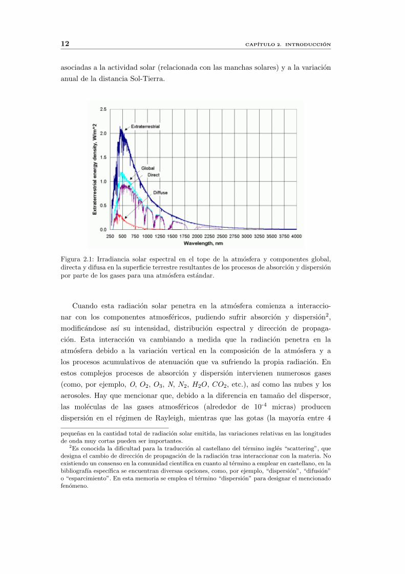
Esa radiacion emitida por el sol llega a la parte superior de la atmosfera terrestre

como un haz de rayos aproximadamente paralelos con una distribucion espectral

asimilable, a grandes rasgos, a la de un cuerpo negro a unos 5800 K situado a 1

U.A., denominandose espectro solar “extraterrestre” (Figura 2.1). Este espectro

esta compuesto aproximadamente por un 9 % de radiacion ultravioleta (UV), rayos

X y gamma (menos de 400 nm), un 50 % de radiacion visible (400-750 nm) y un

41 % de radiacion infrarroja (750-4000 nm). Esta radiacion sufre ligeras1 variaciones

1Hay que hacer notar que, aunque las variaciones en la actividad solar producen fluctuaciones

11

12 CAPITULO 2. INTRODUCCION

asociadas a la actividad solar (relacionada con las manchas solares) y a la variacion

anual de la distancia Sol-Tierra.

Figura 2.1: Irradiancia solar espectral en el tope de la atmosfera y componentes global,directa y difusa en la superficie terrestre resultantes de los procesos de absorcion y dispersionpor parte de los gases para una atmosfera estandar.

Cuando esta radiacion solar penetra en la atmosfera comienza a interaccio-

nar con los componentes atmosfericos, pudiendo sufrir absorcion y dispersion2,

modificandose ası su intensidad, distribucion espectral y direccion de propaga-

cion. Esta interaccion va cambiando a medida que la radiacion penetra en la

atmosfera debido a la variacion vertical en la composicion de la atmosfera y a

los procesos acumulativos de atenuacion que va sufriendo la propia radiacion. En

estos complejos procesos de absorcion y dispersion intervienen numerosos gases

(como, por ejemplo, O, O2, O3, N, N2, H2O, CO2, etc.), ası como las nubes y los

aerosoles. Hay que mencionar que, debido a la diferencia en tamano del dispersor,

las moleculas de las gases atmosfericos (alrededor de 10-4 micras) producen

dispersion en el regimen de Rayleigh, mientras que las gotas (la mayorıa entre 4

pequenas en la cantidad total de radiacion solar emitida, las variaciones relativas en las longitudesde onda muy cortas pueden ser importantes.

2Es conocida la dificultad para la traduccion al castellano del termino ingles “scattering”, quedesigna el cambio de direccion de propagacion de la radiacion tras interaccionar con la materia. Noexistiendo un consenso en la comunidad cientıfica en cuanto al termino a emplear en castellano, en labibliografıa especıfica se encuentran diversas opciones, como, por ejemplo, “dispersion”, “difusion”o “esparcimiento”. En esta memoria se emplea el termino “dispersion” para designar el mencionadofenomeno.

2.1. ORIGEN Y CARACTERISTICAS DE LA RADIACION SOLAR DIFUSA 13

y 50 micras) y cristales (entre 1 y 100 micras) de las nubes, y los aerosoles (gran

variedad, entre 10-3 y 102 micras), producen dispersion en el regimen Mie. Este

hecho es importante pues la dispersion Rayleigh presenta una acusada dependen-

cia con la longitud de onda, dispersandose mas las longitudes de onda menores,

mientras que la dispersion Mie por una nube no resulta tan selectiva espectralmente.

Como consecuencia de estos complejos procesos de absorcion y dispersion, acaba

llegando a la superficie terrestre un campo de radiacion solar atenuado respecto al

que incide en el tope de la atmosfera. Este campo radiativo global esta compuesto

por: 1) radiacion solar que no ha sido dispersada en su recorrido dentro de la

atmosfera y que, por tanto, proviene en la direccion del sol (la cual se denomina

radiacion solar directa), y 2) radiacion solar que ha sido dispersada una o varias

veces y que proviene de todas direcciones (la cual se denomina radiacion solar

difusa). Debido a la dependencia espectral de la absorcion y de algunos procesos

de dispersion, la distribucion espectral de la radiacion solar directa y difusa

difieren, aportando interesante informacion sobre dichos procesos de dispersion

y, como consecuencia, sobre los componentes atmosfericos que han intervenido.

Ası, la medida de la radiacion solar difusa en superficie en ciertas longitudes de

onda permite estimar caracterısticas de la columna de aerosol [Gueymard, 1998;

Foyo-Moreno et al., 2014] y de la nubosidad [Long and Ackerman, 2000; Kaskautis

et al., 2008]. Ademas, la medida de la particion del campo radiativo solar en su

componentes directa y difusa resulta esencial para numerosas aplicaciones, como el

aprovechamiento del recurso solar como fuente de energıa renovable.

La Figura 2.1 presenta un ejemplo de la atenuacion que sufre la radiacion solar

al atravesar la atmosfera. Dicha figura muestra la irradiancia solar espectral global

(directa mas difusa), directa y difusa que llega a la superficie terrestre suponiendo

una atmosfera estandar sin nubes ni aerosoles, suelo con reflectividad nula y un

angulo cenital solar de 42°. Como puede observarse, la radiacion que finalmente

llega a la superficie terrestre abarca longitudes de onda comprendidas entre los 290

nm y los 4000 nm. A la radiacion solar integrada en todo este intervalo espectral

se la denomina radiacion solar total3. Este intervalo espectral incluye longitudes

de onda del rango ultravioleta (280 nm - 400 nm), visible (400 nm - 700 nm) e

infrarrojo (700 - 4000 nm). Se observa ademas un mayor peso de la componente

difusa para las longitudes de onda mas cortas, lo cual se debe a su mayor dispersion

3En la bibliografıa se emplean indistintamente los terminos “total” y “global ”para designarla radiacion solar integrada a todo el espectro solar. En esta memoria se prefiere utilizar “total”,reservando el termino “global” para referirse a la suma de las componentes directa y difusa de laradiacion.


por las moleculas de los gases atmosfericos. En la figura tambien se advierte el

importante papel de los gases atmosfericos en los procesos de absorcion, entre los

que destacan el ozono (para las longitudes de onda mas cortas) y el vapor de agua

(numerosas bandas de absorcion a partir de 0.5 micras).

La atenuacion de la radiacion solar por parte de la atmosfera para una localiza-

cion concreta varıa contınuamente dependiendo de la geometrıa de iluminacion solar,

los perfiles de concentracion de los gases, y de la presencia, distribucion espacial y

caracterısticas radiativas de nubes y aerosoles. En el caso de cielo despejado acaba

llegando a la superficie terrestre un valor global promedio en torno al 68 % de la

radiacion solar incidente en el tope de la atmosfera. En el caso de cielo totalmente

cubierto el porcentaje global promedio ronda el 28 %. Estos grandes numeros solo

pretenden dar una idea de la importancia de las nubes en este proceso de atenuacion,

pues cada situacion concreta ha de ser analizada de forma particular, teniendo gran

importancia la forma y distribucion espacial tridimensional de las nubes, su posicion

relativa respecto del sol, las propiedades radiativas de las gotas, la distribucion de

tamanos de gota dentro de la nube y su variacion con la altura y con la cercanıa a

los bordes de la nube, la existencia de distintas fases lıquida y solida dentro de una

misma nube, etc. Como ejemplo basta mencionar que, bajo condiciones de nubes

rotas, la reflexion de la radiacion en las paredes de las nubes puede dar lugar a

una focalizacion de la radiacion en distintas areas del suelo, dando lugar a valores

locales de radiacion superiores incluso a los correspondientes a la radiacion solar en

el tope de la atmosfera [Cede et al., 2002; Sabburg and Calbo, 2009; Piedehierro et

al., 2014].

2.2. Aplicaciones

2.2.1. Energıa solar

Ademas de su papel fundamental en los procesos climaticos y biologicos, la

radiacion solar constituye una fuente casi inagotable de energıa. La energıa solar

sobre la superficie terrestre es 10000 veces mayor que la demanda anual de energıa

mundial. La sociedad cientıfica Union of Concerned Scientists sostiene que solo 18

dıas de irradiacion solar sobre la Tierra contienen la misma cantidad de energıa que

la acumulada por todas las reservas mundiales actuales de carbon, petroleo y gas

natural. Ası, la energıa solar constituye una prometedora alternativa a las fuentes

de energıa mas utilizadas actualmente, pudiendo contribuir ademas a un desarrollo

mas global y sostenible.

2.2. APLICACIONES 15

La disponibilidad del recurso solar varıa de manera importante con la latitud,

continentalidad y condiciones meteorologicas de cada localizacion. Uno de los

aspectos decisivos para el correcto aprovechamiento de dicho recurso solar es

conocer la particion del campo radiativo en sus componentes directa y difusa.

Esta informacion es esencial para el diseno del sistemas de aprovechamiento solar

adecuados a cada localizacion y condiciones atmosfericas [Posadillo et al., 2009; El-

Sebaii et al., 2010; Torres et al. 2010].

En la actualidad existen dos tipos principales de tecnologıa para aprovechar

la energıa solar: termosolar y fotovoltaica. La primera de ellas consiste en utilizar

la radiacion solar de forma directa para producir calor mediante captadores

o colectores termicos. Dicho calor puede aprovecharse para cocinar alimentos,

calentar agua para el consumo domestico o para generar energıa mecanica y, a

partir de ella, energıa electrica. Por otro lado, la tecnologıa fotovoltaica consiste en

transformar la radiacion solar en energıa electrica mediante el uso de dispositivos

basados en semiconductores o en una deposicion de metales sobre un cierto sustrato.

Ambas formas de aprovechamiento de la energıa solar se basan en la incidencia de

la radiacion solar sobre ciertos dispositivos, lo que requiere el conocimiento preciso

de la particion de la radiacion solar en sus componentes directa y difusa. Ası, por

ejemplo, la tecnologıa fotovoltaica es mas adecuada en aquellas regiones en las que la

componente difusa es la predominante. Por el contrario, en las zonas con predominio

de la componente directa, la tecnologıa termosolar de concentracion presenta un

mayor rendimiento.

2.2.2. Arquitectura solar

Ademas de sus aplicaciones a gran escala para la generacion de calor o energıa

electrica, la energıa solar se ha hecho un hueco relevante en otras areas como

la arquitectura. Dentro de esta disciplina se ha desarrollado la rama conocida

como Arquitectura Solar que emplea tecnicas para aprovechar la energıa solar en

las edificaciones. Para ello resulta fundamental conocer la radiacion solar y su

distribucion en las componentes difusa y directa en cada localizacion, con el fin de

dimensionar, orientar y disenar edificios que aprovechen la energıa solar de forma

mas eficiente.

Lejos de ser un movimiento reciente, las primeras tecnicas de aprovechamiento


solar en edificios datan de la Antigua Grecia. Algunas de esas tecnicas como orien-

tar los edificios al sol, seleccionar materiales con propiedades termicas favorables,

disenar espacios por los que el aire circule de forma natural o usar voladizos, toldos

y vegetacion con el fin de generar sombra, siguen siendo utilizadas en la actualidad.

Este conjunto de tecnicas que permiten en uso y control de la energıa solar de for-

ma directa, sin transformarla, se denomina tecnologıa solar pasiva. Existe otro tipo

de tecnologıa solar, denominada tecnologıa solar activa, que transforma la energıa

solar en energıa electrica o mecanica. Un ejemplo de este tipo de tecnologıa son la

mayorıa de los sistemas de agua caliente sanitaria. En la actualidad, lo mas habitual

es formar sistemas hıbridos que combinan el bajo coste de mantenimiento de los

sistemas pasivos y el mayor rendimiento de los sistemas termicos activos.

2.2.3. Salud

A pesar de suponer tan solo un 5 % del intervalo total de la radiacion solar que

finalmente llega al suelo, la radiacion UV juega un papel fundamental en numerosos

procesos biologicos, ecologicos y fotoquımicos. En este intervalo espectral la compo-

nente difusa supone una gran contribucion. Ası, debido a la mayor efectividad de

los procesos de dispersion para las longitudes de onda mas cortas, al menos el 40 %

de la radiacion UV que llega a la superficie terrestre lo hace en forma de radiacion

difusa [Utrillas et al., 2007].

En principio, una dosis adecuada de radiacion UV resulta muy beneficiosa para

la salud de los seres humanos ya que promueve la sıntesis de vitamina D3, ayuda

a mantener los niveles de calcio en la sangre y fortalece el sistema inmunitario

[Webb et al., 1988; Glerup et al., 2000; Holick, 2004]. Sin embargo, una exposicion

excesiva puede tener consecuencias muy negativas, contribuyendo al debilitamiento

del sistema inmune, propiciando el desarrollo de trastornos oculares como las

cataratas, y favoreciendo la aparicion de de eritema4 y el desarrollo de canceres de

piel [Diffey, 2004; Heisler, 2010]. Para medir los efectos de la radiacion UV sobre

los seres humanos, en particular su capacidad para producir eritema en la piel

humana, se utiliza el conocido como espectro de accion eritematica [McKinlay y

Diffey, 1987; CIE, 1998]. A la radiacion UV ponderada por este espectro de accion

se la denomina radiacion ultravioleta eritematica (UVER).

La preocupacion por los efectos daninos de la radiacion UV sobre la salud

humana se ve acentuada por el importante peso que la componente difusa tiene en

4Enrojecimiento de la piel

2.3. RADIACION SOLAR DIFUSA EN EL MARCO DEL CAMBIO CLIMATICO ACTUAL 17

este intervalo espectral. Ademas de suponer un elevado porcentaje de la radiacion

global UV que llega a la superficie terrestre, la radiacion difusa UV llega a la

superficie procedente de todas direcciones, lo que dificulta su bloqueo. Ası por

ejemplo, la irradiancia UVER difusa bajo una sombrilla de playa estandar puede

alcanzar el 34 % de la irradiancia UVER global [Utrillas et al., 2010] y hasta el 60 %

bajo la sombra de un arbol [Parisi et al., 2000].

Con el fin de informar y concienciar a la ciudadanıa sobre la importancia de

la radiacion UV y de sus posibles efectos nocivos para la salud, las autoridades

sanitarias de numerosos paıses han promovido la difusion del denominado Indice

Ultravioleta, UVI [ICNIRP, 1995]. Se trata de una informacion sencilla y facil de

entender que resume en un unico numero el nivel de radiacion solar UVER que

llega a la superficie terrestre. Este ındice fue estandarizado por la Organizacion

Mundial de la Salud en su Guıa “Indice UV” [WHO, 2003], en la cual se incluyen,

ademas, recomendaciones sobre como protegerse de la radiacion solar UV.

Ademas de su influencia sobre el ser humano, la radiacion UV tiene importantes

efectos sobre la salud de numerosos ecosistemas. Por ejemplo, el exceso de radiacion

UV induce una disminucion de la produccion de biomasa (plantas, fitoplancton y

zooplancton) lo que puede conducir a una reduccion de la capacidad de fijacion de

dioxido de carbono [Zepp et al., 2008]. Ademas, la cantidad de radiacion UV deter-

mina los patrones de migracion y la pigmentacion de algunas especies de zooplancton

[Hader et al., 2011, 2015]. Varios estudios han demostrado tambien que en la etapa

larval de algunos peces, la radiacion UV puede influir en su desarrollo, aumentar

las tasas de mutacion, o causar danos en la piel y los ojos y, por tanto, afectar a su

capacidad de supervivencia [Hader et al., 2011, 2015].

2.3. Radiacion solar difusa en el marco del cambio

climatico actual

La cambiante actividad humana ha provocado alteraciones importantes en la

composicion de la atmosfera [Blumthaler et al 1994; Herman, 2010; Bais et al.,

2011], aumentando significativamente la abundancia de algunos gases (como el CO2,

CH4, NO2, etc.) y de los aerosoles. Este cambio en la composicion atmosferica

afecta notablemente a los procesos de absorcion y dispersion, modificando la

distribucion de la radiacion solar en sus componentes difusa y directa. A su vez,

estos cambios en el campo radiativo solar conllevan una modificacion del balance

radiativo y, en consecuencia, del clima.


Las primeras evidencias de las variaciones seculares en la radiacion solar en

la superficie de la Tierra fueron detectadas a finales de 1980 y principios de 1990

[Ohmura y Lang, 1989; Dutton et al., 1990]. Desde entonces, numerosos estudios

han analizado la tendencia de la irradiancia solar global media en la superficie

de la Tierra [Wild, 2009]. Wild et al. [2005] cuantificaron que estas variaciones se

encontraban entre -5.1 W/m2 y -1.6 W/m2 por decada durante el perıodo 1960-1990

y entre +2.2 W/m2 y +5.1 W/m2 por decada a partir de 1990. Esta tendencia

ha sido confirmada por estudios posteriores [Sanchez-Lorenzo et al., 2015; Wild,

2016]. Sin embargo, el responsable de este cambio no esta claro, y por lo tanto, la

contribucion de las nubes y los aerosoles a las variaciones decadales de la irradiancia

solar global sigue siendo un tema controvertido [Wild, 2009; Augustine y Dutton,

2013; Mateos et al., 2014].

Tambien se han detectado variaciones en las componentes individuales de la

radiacion solar y en subintervalos espectrales. Ası, recientemente se han detectado

tendencias en los valores de radiacion solar difusa total y tambien especıficamente

en su rango UV. Ası, se ha observado una tendencia positiva de +3 W/m2 por

decada en los valores de radiacion solar difusa total en Estados unidos durante

el periodo 1996-2007 [Long et al., 2009]. Tambien se han detectado tenden-

cias negativas, como en Girona (Espana), donde un estudio reciente cuantifica

la tendencia en -1.3 W/m2 por decada para el periodo 1994-2014 [Calbo et al., 2016].

En cuanto al rango UV, los estudios indican la existencia de tendencias positivas

en Europa [Krzyscin et al., 2011; Smedley et al., 2012]. En el caso particular de

la Penınsula Iberica se ha detectado una tendencia de +2.1 % por decada en los

valores de irradiancia UVER en el perıodo 1985-2011 [Roman et al., 2015].

Estas alteraciones en los valores de radiacion difusa total y UV tienen importan-

tes consecuencias sobre los ecosistemas. Varios estudios han senalado que existe una

estrecha relacion entre la cantidad de radiacion difusa total y la fotosıntesis, aumen-

tando generalmente su eficiencia cuando la radiacion difusa total aumenta [Mercado,

2009; Kannianh, 2012]. Sin embargo, la sobreexposicion a la radiacion UV reduce el

tamano, productividad y calidad en muchas de las especies de plantas de cultivo el

arroz, la soja, el trigo, el algodon o el maız. El aumento de la radiacion UV tambien

implica la reduccion de las poblaciones de fitoplancton y la extincion de importantes

ecosistemas como los corales [Lesser y Farrell, 2004].

2.4. MEDIDA DE LA RADIACION SOLAR DIFUSA 19

2.4. Medida de la radiacion solar difusa

La medida de la radiacion solar difusa descansa en la caracterıstica diferen-

ciadora de la componente difusa respecto a la directa: que la primera proviene de

todas direcciones mientras que la segunda llega solamente en la direccion solar.

Por ello, para medir la componente difusa se emplean los mismos instrumentos que

para la medida de radiacion solar global pero se requiere, ademas un dispositivo de

apantallamiento que impida que la componente directa llegue a dicho sensor. Este

requisito adicional sobre la instrumentacion explica que la medida de la componente

difusa este mucho menos extendida que la medida de la radiacion global. Esta menor

abundancia de medidas de la componente difusa es muchısimo mas acentuada en el

caso del rango UV.

Esta situacion esta cambiando actualmente pues el interes por la medida de la

radiacion difusa total ha aumentado notablemente debido a la necesidad de un cono-

cimiento mas detallado del balance radiativo y a sus implicaciones para el desarrollo

de tecnologıas para el aprovechamiento de la energıa solar. Entre las iniciativas para

la medida de la radiacion difusa total hay que senalar los programas como la Base-

line Surface Radiation Network (BSRN) o el Atmospheric Radiation Measurements

(ARM). A pesar de ello, el numero de estaciones en las que se mide irradiancia solar

difusa ultravioleta sigue siendo muy escas. Entre el reducido numero de estudios que

aportan medidas experimentales de irradiancia solar difusa ultravioleta eritemati-

ca destacan los desarrollados en Australia [Parisi et al., 2000; Turnbull et al., 2005;

Turnbull and Parisi, 2008], Valencia [Utrillas et al., 2007, 2009; Utrillas, 2010; Nunez

et al., 2012].

2.4.1. Radiometros de banda ancha para la media de irradiancia

difusa total y ultravioleta

Existen diferentes magnitudes radiometricas relacionadas con la radiacion. En

el caso de la medida de la radiacion solar difusa la magnitud mas interesante es la

irradiancia. Esta se define como la energıa radiante que llega a una superficie por

unidad de tiempo y por unidad de superficie. Podemos decir que se trata pues de

una densidad superficial (por unidad de superficie) de potencia (energıa por unidad

de tiempo). Sus unidades en el Sistema Internacional son W/m2. En el caso de la

medida meteorologica estandar de la irradiancia solar global y difusa se considera

una superficie horizontal5, por lo que los radiometros deben estar bien nivelados.

5Para algunos objetivos particulares puede resultar interesante medir la irradiancia sobre super-ficies inclinadas, por lo que los instrumentos de medida pueden colocarse inclinados, paralelos a la


Existen distintos tipos de instrumentos para medir la irradiancia solar sobre

la superficie terrestre segun el rango y la resolucion espectral que se desean

medir. Atendiendo a esta ultima caracterıstica los instrumentos se clasifican en: 1)

espectrorradiometros, los cuales proporcionan valores espectrales, 2) radiometros

multicanal, aquellos que miden valores de irradiancia en varias bandas estrechas,

y 3) radiometros de banda ancha, los cuales permiten medir valores de irradiancia

integrados en un amplio intervalo de longitudes de onda.

En esta Tesis Doctoral nos centraremos en el analisis de la irradiancia medida

medidos con instrumentos de banda ancha correspondientes tanto a todo el espectro

solar como exclusivamente al rango ultravioleta. Los radiometros de banda ancha

son instrumentos muy robustos adecuados para la medida automatica durante

largos periodos sometidos a todo tipo de condiciones atmosfericas. Su facil manejo

y mantenimiento y su precio relativamente economico han favorecido la integracion

de este tipo de instrumentos en estaciones radiometricas repartidas por todo el

mundo.

El radiometro utilizado para medir irradiancia solar global o difusa del espectro

solar total recibe el nombre especıfico de piranometro. Los piranometros utilizados

en esta Tesis Doctoral basan su principio de funcionamiento en el efecto termo-

electrico conocido como efecto Seebeck. La parte visible del sensor es una superficie

rugosa pintada de negro que absorbe la radiacion incidente calentandose. Esta

superficie esta en contacto con uno de los extremos de un termopar (union caliente)

que se calienta a su vez. Mientras tanto,el otro extremo del termopar permanece a

un temperatura mas frıa (union frıa) en contacto con el cuerpo del piranometro.

Esta diferencia de temperatura entre ambos extremos de la union termoelectrica

genera una diferencia de potencial que es lo que se registra, y que es proporcional

a la radiacion solar incidente. Para proteger el sensor de influencias externas como

la lluvia, la suciedad o el viento, el piranometro posee una doble cupula de vidrio

transparente que permite la transmision del 98 % de la radiacion solar en todas sus

longitudes de onda.

En el caso de la medida de radiacion ultravioleta los radiometros deben muy

sensibles y precisos ya que la cantidad de radiacion llega a la superficie terrestre en

estas longitudes de onda es varios ordenes de magnitud menor que en longitudes de

onda superiores correspondientes al espectro visible. En los estudios realizados en

esta Tesis Doctoral sobre la radiacion en este intervalo espectral se han utilizado

superficie en cuestion.


radiometros UVS-E-T fabricados por Kipp & Zonen. Este instrumento tiene una

respuesta espectral que simula el espectro de accion eritematica de la piel humana

[ISO 17166:1999/CIE S007/E-1998]. El funcionamiento es algo mas complejo que

en los piranometros. La radiacion solar atraviesa la cupula de cuarzo que permite

el paso del rango UV. Un filtro absorbe la luz visible e IR y deja pasar los la

radiacion correspondiente al espectro de accion CIE. La radiacion UV transmitida

incide sobre una lamina de fosforo sensible a la radiacion UV. Este material

absorbe la componente UV y la reemite por fluorescencia en el rango visible,

predominantemente en longitudes de onda correspondientes al verde [Robertson,

1972; Berger, 1976)]. Un segundo filtro de vidrio transmite la luz reemitida, la cual

es medida por un fotodiodo de estado solido, cuya respuesta maxima esta en el

verde. Todo este dispositivo se encuentra estabilizado a 25 °C para evitar que su

funcionamiento se vea alterado por factores externos.

Todos los instrumentos utilizados en esta Tesis Doctoral satisfacen los estandares

de medida establecidos por la Organizacion Meteorologica Mundial (OMM) para la

medida de irradiancia difusa total y UV, respectivamente [WMO, 2014].

2.4.2. Dispositivos para el bloqueo de la radiacion solar directa.

Como se indico anteriormente en la introduccion de esta seccion, para medir

radiacion difusa se necesita un dispositivo adicional que bloquee la radiacion

procedente de la direccion del Sol impidiendo que llegue al sensor. El primer

mecanismo disenado con este objetivo fue el anillo o banda de sombra. Como su

propio nombre indica, este dispositivo consiste en un anillo o banda que se dispone

paralelo a la trayectoria solar de tal forma que sombrea el sensor del piranometro

durante el movimiento diurno del sol.

El primer modelo de este mecanismo fue fabricado a mediados del siglo pasado

por Drummond y Kristen [1951] y se muestra en la Figura 2.2a. Las series de

irradiancia difusa mas longevas cuentan con medidas obtenidas empleando este

dispositivo. En la actualidad su diseno sigue siendo fundamentalmente el mismo. Los

fabricantes actuales solo han anadido ligeros cambios como la introduccion de dos

brazos moviles que facilitan el manejo del anillo, o la modificacion de su perfil para

que la sombra que se proyecta sobre el sensor sea aproximadamente constante a lo

largo del ano. Un ejemplo es el anillo de sombra CM121 fabricado por Kipp & Zonen

que se muestra en la Figura 2.2b. No obstante, la necesidad de medir radiacion sobre


superficies inclinadas, principalmente de la mano del desarrollo de tecnologıa para

el aprovechamiento de la energıa solar, ha dado lugar a innovadores disenos como el

desarrollado por Simon et al. [2015] que se muestra en la Figura 2.2c. Este dispo-

sitivo permite la medida simultanea de irradiancia difusa en cuatro planos verticales.

(a) (b) (c)

Figura 2.2: Distintos modelos de anillo de sombra. (a) Modelo original de Drummond yKristen [1951] (b) Modelo CM121 fabricado por Kipp & Zonen. (c) Dispositivo de sombradisenado por de Simon et al. [2015] para la medida simulatanea de irradiancia difusa encuatro planos verticales

El anillo de sombra presenta algunas ventajas sobre otros sistemas que hacen

que su uso siga siendo muy extendido en la actualidad. Se trata de un instrumento

facil de operar ya que solo requiere el ajuste manual de su altura con el fin de

adaptarlo a la declinacion solar del dıa en cuestion. La frecuencia con que debe

ajustarse esta altura depende de la epoca del ano y de la latitud de la estacion.

Ademas, su gran robustez hace que sea el dispositivo mas adecuado para la medida

de irradiancia difusa en localizaciones con condiciones meteorologicas extremas,

como en la Antartida [Serrano et al., 2002]. Otra importante ventaja anteriormente

mencionada es la posibilidad de ser adaptado para medir irradiancia difusa sobre

superficies inclinadas.

Los nuevos avances tecnologicos han permitido el desarrollo de dispositivos de

sombreado mas sofisticados. En la actualidad, se ha extendido el uso de seguidores

solares equipados con bolas o discos de sombra (Figura 2.3). Estos dispositivos

consisten en un cuerpo motorizado con unos brazos moviles acabados en una bola


(o disco) que se mueven solidarios al sol en su movimiento diurno, corrigiendo la

altura de las bolas de forma que el sensor del piranometro permanezca sombreado

en todo momento.

Figura 2.3: Seguidor solar Solys2 fabricado por Kipp & Zonen

El seguidor solar presenta algunas ventajas respecto al anillo de sombra, como

son su funcionamiento totalmente automatico y la menor fraccion de cielo ocultada

al sensor por parte del apantallamiento. Ası, mientras el seguidor solar bloquea

exclusivamente el disco solar, el anillo de sombra, debido a su diseno, bloquea, no

solo la componente directa, sino tambien la irradiancia difusa interceptada por todo

el angulo solido subtendido por el anillo. Esto conlleva una subestimacion de la

medida de irradiancia difusa que ha de ser corregida. El analisis de este problema y

su correccion sera uno de los objetivos de esta Tesis Doctoral.

2.4.3. Precision en las medidas de irradiancia difusa total y UV

La precision de las medidas de irradiancia difusa vendra determinada tanto por

las caracterısticas del instrumento utilizado (sensibilidad, respuesta angular, etc.) y

su mantenimiento (calibracion, limpieza, control del sombreado, etc.), ası como por

las caracterısticas del dispositivo de sombreado.

La Organizacion Meteorologica Mundial, a traves de los estudios realizados por

la BSRN, establece que los valores de irradiancia difusa mas precisos son aquellos

medidos por un piranometro ventilado instalado en un seguidor solar (de dos ejes)


y sombreado por un disco o bola que proyecte una sombra de 5° desde el centro

del sensor. Ademas los instrumentos deben ser revisados cada dıa y los datos

deben ser sometidos a un control de calidad. Se estima que la incertidumbre en las

medidas ası obtenidas es de un 2 % (3 W/m2) [Ohmura et al., 1998; McArthur,

2005]. Sin embargo, la mayorıa de las estaciones radiometricas no cuentan con la

instrumentacion y el personal necesario para la aplicacion de un protocolo tan

estricto.

Medir radiacion ultravioleta es difıcil debido a la pequena cantidad de radiacion

en este intervalo espectral que llega a la superficie y a la rapida variacion de esta

cantidad para las distintas longitudes de onda. Debido a ello, el error asociado a la

medida de irradiancia UV es notablemente superior al error de la irradiancia total.

No contribuye a mejorar este panorama las dificultades en la estandarizacion de las

medidas de irradiancia UV debido, principalmente, a la variedad de instrumentos

utilizados para su medida y a los numerosos usos para los que se emplean las me-

didas [WMO, 2003]. La OMM [2014] establece una error del 10 % en el proceso de

calibracion de los radiometros de banda ancha UV. Los radiometros UV utilizados

en esta Tesis Doctoral han sido calibrados siguiendo el procedimiento establecido

por Grupo de Trabajo 4 de la Accion COST 726 [Webb et al., 2006; Grobner et al.

2007; Vilaplana et al., 2009]. Al igual que en el caso de la irradiancia difusa total

tambien el sistema utilizado para sombrear el sensor podrıa ampliar la incertidumbre

las medidas de irradiancia difusa ultravioleta.

2.5. Modelizacion de la radiacion solar difusa

A pesar del incremento en el numero de estaciones radiometricas que incorporan

la instrumentacion necesaria para la medida de la radiacion difusa total, su

distribucion espacial es muy irregular. La situacion es aun mas crıtica en el caso

de las medidas de radiancia difusa ultravioleta. Sin embargo, la componente difusa

depende de variables medidas de forma rutinaria en estaciones radiometricas y

meteorologicas distribuidas por todo el planeta, lo que hace interesante el desarrollo

de modelos que permitan su estimacion a partir de las medidas disponibles.

Asimismo, la modelizacion de la radiacion difusa constituyen una potente

herramienta para entender los complejos procesos que dan lugar a su formacion.

Los modelos permiten analizar el papel de los distintos constituyentes atmosfericos

en los procesos de dispersion ası como los posibles efectos derivados de variaciones

de dichos constituyentes. La simulacion de radiacion solar, y en particular de la

2.5. MODELIZACION DE LA RADIACION SOLAR DIFUSA 25

componente difusa, es fundamental para entender el cambio climatico y sus posibles

efectos sobre los seres vivos. Ademas de su aplicacion a estudios climaticos, los

modelos de radiacion solar difusa son fundamentales en el avance sostenible de las

energıas renovables, la arquitectura, la ingenierıa, la agricultura y la ecologıa.

Los modelos para la estimacion de radiacion solar pueden clasificarse en dos

categorıas: 1) modelos de transferencia radiativa y 2) modelos empıricos. Como

su propio nombre indica, en los modelos de transferencia radiativa, los valores de

radiacion se obtienen mediante la resolucion de las ecuaciones de transferencia

radiativa. El metodo utilizado para resolver dichas ecuaciones y las aproximaciones

consideradas determinaran el tipo de modelo dentro de esta categorıa (1D, 3D,

MonteCarlo, etc.). Estos modelos permiten la estimacion de radiacion solar global,

difusa y directa, espectral o integrada, a diferentes alturas dentro de la atmosfera.

Algunos de los modelos de transferencia radiativa mas empleados por la comunidad

cientıfica son: SBDART, libRadtran o TUV.

Por su parte, los modelos empıricos se construyen mediante el ajuste matematico

de valores de radiacion y datos de los distintos factores que la modulan en su

camino hacia la superficie terrestre. Las formas funcionales y variables implicadas

dependen tanto de la componente de la radiacion que se desea modelizar como de

las variables a partir de las cuales se construira el modelo. En el caso particular

de la componente difusa, entre otros parametros, resulta imprescindible introducir

en el modelos informacion sobre la posicion solar y la capa de aerosoles y/o

nubes. Entre las expresiones empıricas para la estimacion de irradiancia difusa

total se encuentran los modelos Iqbal-C [Iqbal, 1983], REST2 [Gueymard, 2008]

o el modeleo por Boland et al. [2008]. Aunque mucho menos numerosos, tambien

se han propuesto para la estimacion de la irradiancia difusa ultravioleta entre

los que destacan los modelos Grant and Gao [2003], Nunez et al. [2012] y Silva [2015].

De particular interes resultan los modelos empıricos para la obtencion de la frac-

cion de irradiancia difusa, kd, que se define como el cociente entre la irradiancia

difusa y global sobre una superficie horizontal. Trabajar con esta magnitud en lu-

gar de con los valores de irradiancia difusa supone algunas ventajas entre las que

destacan: 1) su menor dependencia con la posicion solar y 2) su mayor sensibilidad

ante pequenas variaciones en la particion difusa/directa de la radiacion solar [Long

y Ackerman, 2000]. Este tipo de modelos toman como variable principal los valores

de transmisividad de la radiacion global en el correspondiente rango de longitudes

de onda. Esta magnitud, que se define como el cociente entre la radiacion global


sobre una superficie horizontal y la radiacion en el tope de la atmosfera, resulta de

gran interes ya que se ve afectada por los mismos procesos de absorcion y dispersion

que la fraccion de difusa. Estos modelos pueden introducir ademas otras variables

que complementen la informacion contenida en el ındice de claridad.

Bibliografıa

Augustine, J. A., and E. G. Dutton (2013), Variability of the surface radiation

budget over the United States from 1996 through 2011 from high-quality measure-

ments, J. Geophys. Res. Atmos., 118, 43–53.

Bais A.F., K.Tourpali, A. Kazantzidis, H. Akiyoshi, S. Bekki, P. Braesicke, M.P.

Chipperfield, M. Dameris, V. Eyring, H. Garny, D. Iachetti, P. Jockel, A. Kubin, U.

Langematz, E. Mancini, M. Michou, O. Morgenstern, T. Nakamura, P.A. Newman,

G. Pitari, D.A. Plummer, E. Rozanov, T.G. Shepherd, K. Shibata, W. Tian,

and Y. Yamashita (2011), Projections of UV radiation changes in the 21st cen-

tury: impact of ozone recovery and cloud effects, Atmos. Chem. Phys., 11, 7533-7545.

Berger, D.S. (1976), The sunburning ultraviolet meter: design and performance,

Photochemistry and Photobiology, 24, 587-593.

Blumthaler, M., W. Ambach, and M. Salzgeber (1994), Effects of cloudiness on

global and diffuse UV irradiance in a high-mountain area, Theor. Appl. Climatol.,

50, 23–30, 1994.

Boland, J., B. Ridley, and B. Brown (2008), Models of diffuse solar radiation,

Renew. Energy, 33, 575–584.

Cede, A., M. Blumthaler, E. Luccini, R.D. Piacentini, L. Nunez (2002). Effects of

clouds on erythemal and total irradiance as derived from data of the Argentine

Network, Journal of Geophysical Research, 29, 2223.

Calbo, J., J.A. Gonzalez, and A. Sanchez-Lorenzo (2016), Building global and

diffuse solar radiation series and assessing decadal trends in Girona (NE Iberian

Peninsula), Theor. Appl. Climatol..

CIE (1998), Erythema reference action spectrum and standard erythema dose,

Vienna, ISO 17166:1999/CIE S007-1998.


de Simon-Martın M., C. Alonso-Tristan, D. Gonzalez-Pena, M. Dıez-Mediavilla

(2015), New device for the simultaneous measurement of diffuse solar irradiance on

several azimuth and tilting angles, Solar Energy, 19, 370-382.

Diffey B.L. (1991), Solar ultraviolet radiation effects on biological systems, Phys.

Med. Biol., 36, 299-328.

Diffey, B. L. (2004), Climate change, ozone depletion and the impact on ultraviolet

exposure of human skin, Phys. Med. Biol., 49, 1–11.

Drummond, A. J. and M. K. Kristen (1951) The measurement of solar radiation in

South Africa, South African J. Sci., 48, I03.

Dutton, E. G., R. S. Stone, D. W. Nelson, and B. G. Mendonca (1990), Recent

interannual variations in solar radiation cloudiness, and surface temperature at the

South Pole, J. Clim., 4, 848–858.

El-Sebaii A. A. and A. Terabia (2003), Estimation of horizontal diffuse solar radia-

tion in Egypt, Energy Conversion & Management, 44, 2471-2482.

Foyo-Moreno,I.,I.Alados,M.Anton, J. Fernandez-Galvez, A. Cazorla, and L.

Alados-Arboledas (2014), Estimating aerosol characteristics from solar irradiance

measurements at an urban location in southeastern Spain, J. Geophys.Res. Atmos.,

119,1845-1859.

Glerup, H., K. Mikkelsen, L. Poulsen, E. Hass, S. Overbeck, and J. Thomsen (2000),

Commonly recommended daily intake of vitamin D is not sufficient if sunlight

exposure is limited, J. Intern. Med., 247, 260–268.

Grant, R. H., and W. Gao (2003), Diffuse fraction of UV radiation under partly

cloudy skies as defined by the Automated Surface Observation System (ASOS), J.

Geophys. Res., 108(D2), 4046.

Grobner, J., G. Hulsen, L. Vuilleumier, M. Blumthaler, J. M. Vilapla-

na, D. Walker, and J. E. Gil (2007), Report of the PMOD/WRC-COST

Calibration and Intercomparison of Erythemal radiometers. Available at:

http//i115srv.vuwien.ac.at/uv/COST726/COST726 Dateien/Results/PMOD

WRC COST726 campaign 2006 R.pdf.


Gueymard C., F. Vigola (1998), Determination of atmospheric turvidity fromm the

diffuse-eam broadband irradiance ratio, Solar Energy, 63, 135–146.

Gueymard, C.A. (2008), REST2: High performance solar radiation model

for cloudless-sky irradiance, illuminance and photosynthetically active radia-

tion—validation with a benchmark dataset, Solar Energy, 82, 272–285.

Hader D.P., E.W. Helbling, C.E. Williamson, and R.C. Worrest (2011), Effects

of UV radiation on aquatic ecosystems and interactions with climate change,

Photochem. Photobiol. Sci., 10, 242 -260.

Hader D.P., C.E. Williamson, S.A. Wangberg, M. Rautio, K.C. Rose, K. Gao,

E.W. Helbling, R.P. Sinha, R.C. Worrest (2015), Effects of UV radiation on

aquatic ecosystems and interactions with other environmental factors, Photochem.

Photobiol. Sci., 14, 108-126.

Heisler, G. M. (2010), Urban forest influence on exposure to UV radiation and po-

tential consequences for human health, in UV Radiation in Global Climate Change.

Measurements, Modeling and Effects on Ecosystems, edited by Gao, W., et al., pp.

331–369, Tsinghua University Press, Beijing.

Herman, J. R. (2010), Global increase in UV irradiance during the past 30 years

(1979–2008) estimated from satellite data, J. Geophys. Res., 115.

Holick, M. F. (2004), Vitamin D: importance in the prevention of cancers, type 1

diabetes, heart disease and osteoposoris, Am. J. Clin. Nutr., 79, 362–371.

Iqbal, M., (1983), An Introduction to Solar Radiation, Academic Press, Toronto.

ICNIRP (1995), Global Solar UV Index. WHO/WMO/INCIRP recommendation,

INCIRP publication no 1/95, Oberschleissheim.

Kaskaoutis D.G., H.D. Kambezidis, S.K. Kharol, K.V.S. Badarinath (2008), The

diffuse-to-global spectral irradiance ratio as a cloud-screening technique for ra-

diometric data, Journal of Atmospheric and Solar-Terrestrial Physics, 70,1597-1606.

Krzyscin J.W., P.S. Sobolewski, J. Jaroslawski, J. Podgorski, and B. Rajewska-

Wiech (2011), Erythemal UV observations at Belsk, Poland, in the period

1976–2008: Data homogenization, climatology, and trends, Acta Geophysica, 59,


155-182.

Long C.N., and T.P. Ackerman (2000),Identification of clear skies from broadband

pyranometer measurements and calculation of downwelling shortwave cloud effects,

Journal of Geophysical Research, 105, 609-615.

Long, C.N., E.G. Dutton, J. A. Augustine, W. Wiscombe, M. Wild, S. A. Mc-

Farlane, and C. J. Flynn, (2009), Significant decadal brightening of downwelling

shortwave in the continental United States, J. Geophys. Res., 114.

Mateos, D., A. Sanchez-Lorenzo, M. Anton, V. E. Cachorro, J. Calbo, M. J. Costa,

B. Torres, and M. Wild (2014), Quantifying the respective roles of aerosols and

clouds in the strong brightening since the early 2000s over the Iberian Peninsula, J.

Geophys. Res. Atmos., 119.

McArthur L. J. B. (2005), Baseline Surface Radiation Network (BSRN). Operations

Manual, Version 2.1. WCRP-121, WMO/TD-No. 1274

McKinlay A.F. and B.L. Diffey (1987), Human Exposure to Ultraviolet Radiation:

Risks and Regulations Edited by W. F. Passchier and B. F. M. Bosnajakovic,

pp.83–87, Elsevier, Amsterdam.

Nunez, M., M. P. Utrillas, and J. A. Martinez-Lozano (2012), Approaches to

partitioning the global UVER irradiance into its direct and diffuse components in

Valencia, Spain, J. Geophys. Res., 117.

Ohmura, A., and H. Lang (1989), Secular variation of global radiation over Europe,

in Current Problems in Atmospheric Radiation, edited by J. Lenoble and J. F.

Geleyn, pp. 98–301, Deepak, Hampton, Va.

Ohmura, A. , E. Dutton, B. Forgan, C. Frohlich , H. Gilgen, H. Hegner, A. Heimo,

G. Konig-Langlo, B. Mcarthur, G. Muller, R. Philipona, R. Pinker, C.H. Whitlock,

and M. Wild (1998), Baseline Surface Radiation Network (BSRN/WRMC), a new

precision radiometry for climate research, Bull. Amer. Meteor. Soc., 79, 2115 – 2136.

Parisi, A. V., M. G. Kimlin, J. C. F. Wong, and M. Wilson (2000), Diffuse

component of solar ultraviolet radiation in tree shade , J. Photochem. Photobiol.

Biol., 54, 116–120.


Parisi, A. V., A. Green, and M. G. Kimlin (2001), Diffuse Solar UV Radiation

and Implications for Preventing Human Eye Damage, Photochem. Photobiol., 73,

135–139.

Piedehierro A.A., M. Anton, A. Cazorla, L. Alados-Arboleda L., and F.J. Olmo

(2014), Evaluation of enhancement events of total solar irradiance during cloudy

conditions at Granada (Southeastern Spain), Atmospheric Research, 135-136,1-7.

Posadillo R., R. Lopez Luque (2009), Hourly distributions of the diffuse fraction of

global solar irradiation in Cordoba (Spain), Energy Conversion and Management,

50, 223-231.

Robertson, D.F. (1972). Solar ultraviolet radiation in relation to human sunburn

and skin cancer, Ph. D. thesis, University of Queensland, Australia.

Roman R., J. Bilbao and A. de Miguel (2015), Erythemal ultraviolet irradiation

trends in the Iberian Peninsula from 1950 to 2011, Atmos. Chem. Phys., 15, 375–391.

Sabburg, J., and J. Calbo (2009), Five years of cloud enhanced surface UV

radiation measurements at two sites (in the Northern and Southern Hemispheres),

Atmospheric Research, 93, 902–912.

Sanchez-Lorenzo, A., M. Wild, M. Brunetti, J. A. Guijarro, M. Z. Hakuba, J. Calbo,

S. Mystakidis, and B. Bartok (2015), Reassessment and update of long-term trends

in downward surface shortwave radiation over Europe (1939–2012), J. Geophys.

Res. Atmos., 120, 9555–9569.

Serrano A., M. Anton, M. L. Cancillo, J. A. Garcıa, M. R. Arias, V. L. Mateos,

M. Ramos (2002), Medidas de radiacion solar en la Isla Decepcion (Shetland del

Sur, Antartida) durante el verano austral (campana 2000/2001), Proceedings 3a

Asamblea Hispano-Portuguesa de Geodesia y Geofısica, Valencia (Espana), Tomo

II, 1349-1352, ISBN 84-9705-297-8.

Silva A. (2015), The diffuse component of erythemal ultraviolet radiation, Photo-

chem. Photobiol. Sci.

Smedley A.R.D., J.S. Rimmer, D. Moore, R. Toumi, and A.R. Webb (2012), Total

ozone and surface UV trends in the United Kingdom: 1979–2008, Int. J Climatol.,

32, 338-346.


Torres J.L., De Blas M., Garcıa A., de Francisco A. (2010), Comparative study of

various models in estimating hourly diffuse solar irradiance, Renewable Energy, 35,

1325-1332.

Turnbull, D. J., A. V. Parisi, and M. G. Kimlin (2005), Vitamin D effective

ultraviolet wavelengths due to scattering in shade, J. Steroid Biochem. Mol. Biol.,

96, 431–436.

Turnbull, D. J., and A. V. Parisi (2008), Utilising shade to optimize UV exposure

for vitamin D, Atmos. Chem. Phys., 8, 2841–2846.

Utrillas, M. P., M. J. Marın, A. R. Esteve, F. Tena, J. Canada, V. Estelles, and J.

A. Martınez-Lozano (2007), Diffuse UV erythemal radiation experimental values,

Journal of Geophysical Research, 112

Utrillas, M. P., M. J. Marın, A. R. Esteve, V. Estelles, F. Tena, J. Canada, and J.

A. Martınez-Lozano (2009), Diffuse Ultraviolet Erythemal Irradiance on Inclined

Planes: A Comparison of Experimental and Modeled Data, Phot. Pho., 85(5), 1245.

Utrillas, M. P., J. A. Martınez-Lozano, and M. Nunez (2010), Ultraviolet Radiation

Protection by a Beach Umbrella, Photochem. Photobiol., 86, 449–456.

Vilaplana, J. M., A. Serrano, M. Anton, M. L. Cancillo, M. Parias, J. Grobner,

G. Hulsen, G. Zablocky, A. Dıaz, and B. A. de la Morena (2009), COST Action

726 – Report of the “El Arenosillo”/INTA-COST calibration and intercomparison

campaign of UVER broadband radiometers.

Webb, A. R., L. Kline, and M. F. Holick (1988), Influence of season and latitude

on the cutaneous synthesis of Vitamin D3: exposure to winter sunlight in Boston

and Edmonton will not promote Vitamin D3 synthesis in human skin, J. Clin.

Endocrinol. Metab., 67, 373–378.

Webb, A., J. Grobner, and M. Blumthaler (2006), A practical guide to operating

broadband instruments measuring erythemally weighted irradiance, Produced by

the join efforts of WMO SAG UV and Working Group 4 of the COST-726 Action:

Long Term Changes and Climatology of the UV Radiation over Europe, vol.EUR

22595/WMO.


Wild, M., G. Hans, A. Roesch, A. Ohmura, C. N. Long, E. G. Dutton, B. Forgan, A.

Kallis, V. Russak, and A. Tsvetkov (2005), From dimming to brightening: Decadal

changes in surface solar radiation, Science, 308, 847–850.

Wild, M. (2009), Global dimming and brightening: A review, J. Geophys. Res., 114.

Wild, M. (2016), Decadal changes in radiative fluxes at land and ocean surfaces and

their relevance for global warming, Wiley Interdiscip. Rev.Clim. Change, 7, 91–107.

World Meteorological Organization (2003). Indice UV Solar Mundial: Guıa Practi-

ca (version en castellano), 28 pp. Organizacion Mundial de la Salud (WHO),

Organizacion Meteorologica Mundial (WMO), Programa de las Naciones Unidas

para el Medio Ambiente (UNEP), Comision Internacional de Proteccion contra la

Radiacion no Ionizante (ICNIRP), Ginebra.

World Meteorological Organization (2008), Guide to Meteorological Instruments

and Methods of Observation, vol. 8, 7th ed., 681 pp.,Secretariat of the World

Meteorological Organization, Geneva, Switzerland.

World Meteorological Organization (2014), Guide to Meteorological Instruments

and Methods of Observation, vol. 8, 7th ed., 1128 pp.,Secretariat of the World

Meteorological Organization, Geneva, Switzerland.

Capıtulo 3

Error asociado al cero termico o

“thermal offset”

3.1. Introduccion

Una de las principales fuentes de error en las medidas de irradiancia solar

realizadas por los piranometros es la senal asociada al cero termico (thermal offset,

en su denominacion en ingles). Se denomina cero termico al voltaje que se genera

en el sensor como resultado del flujo neto de radiacion establecido entre este y la

cupula (Figura 3.1). Este voltaje se anade al voltaje correspondiente a la medida de

la radiacion solar, formando parte de la senal de salida. En la mayorıa de los casos

la temperatura del sensor es mayor que la de la cupula, produciendo un voltaje

negativo y, ası, reduciendo la magnitud de la senal final de salida. La no correccion

de esta fuente de error conduce generalmente a una subestimacion de la irradiancia

solar medida.

Estudios previos han estimado que los valores del cero termico se encuentran

entre -20 W/m2 y 0 W/m2 [Bush et al., 2000; Haeffelin et al., 2001]1. Este valor

supera notablemente el lımite de -7 W/m2 aceptado por la OMM en las medidas

de irradiancia global y difusa de calidad. En el caso de la irradiancia solar difusa,

este valor puede llegar a suponer un error de hasta el 40 % [Dutton et al., 2001],

muy por encima del la incertidumbre del 2 % que la establecida por la BSRN para

las medidas de irradiancia difusa total [Ohmura et al., 1998; McArthur, 2005].

El cero termico de cada piranometro es diferente, pues depende de su diseno y

1La bibliografıa correspondiente a la seccion introductoria de cada uno de los capıtulos 2, 3 y 4se encuentra recogida dentro de los artıculos que componen dichos capıtulos.

33

34 CAPITULO 3. ERROR ASOCIADO AL CERO TERMICO O “THERMAL OFFSET”

materiales de construccion. Tambien esta afectado por las configuracion de trabajo

(ventilado o no, sombreado o no) y las condiciones meteorologicas del momento.

Entre las variables meteorologicas que mas influyen se pueden citar, por una parte,

aquellas condiciones que determinan la temperatura del sensor (la propia radiacion

solar que se pretende medir y sus factores moduladores como nubosidad y, en menor

medida, aerosoles), y por otra, aquellas condiciones relacionadas con la temperatura

de la cupula (la velocidad del viento, la temperatura ambiente, la humedad relativa,

etc.). Todo ello hace que el cero termico de un piranometro midiendo en el exterior

varıe continuamente adaptandose al forzamiento de los factores externos.

Figura 3.1: Flujo de radiacion establecido entre el sensor, las cupulas y la atmosfera

A pesar de su importancia y de ser una fuente de error conocida desde hace

bastante tiempo existen numerosos aspectos del cero termico aun sin resolver. A

continuacion se enumeran y describen brevemente los aspectos mas destacados aun

sin resolver sobre el cero termico:

No existe un acuerdo general sobre si el cero termico de un piranometro difiere

significativamente por el hecho de estar midiendo irradiancia global o difusa.

Por un lado, estudios como el realizado por Bush et al. [2000] han detectado

valores del error termico diferentes para un mismo instrumento midiendo global

o difusa. Estos resultados son explicados en base al diferente estado termico en

el que el piranometro trabaja cuando esta sombreado y cuando no lo esta. Por

otros lado, estudios como el desarrollado por Philipona [2002] no han observado

tales diferencias.

Existe una notable controversia sobre la posibilidad de corregir el cero termico

de las medidas diurnas empleando modelos basados en medidas nocturnas.

Algunos autores proponen la utilizacion de la senal nocturna del piranometro

para la correccion del error termico diurno [Dutton et al., 2001; Younkin y

3.1. INTRODUCCION 35

Long, 2004]. Sin embargo, otros autores senalan que esto no es adecuado debido

al importante papel que la radiacion solar tiene en el balance final que genera

el error termico [Cess et al., 2000; Haeffelin et al., 2001].

El efecto de la ventilacion artificial en el cero termico de los piranometros no

esta suficientemente estudiado. En general, se espera que la ventilacion reduzca

la diferencia de temperatura entre las distintas partes del piranometro y, por

tanto, reduzca su cero termico. Sin embargo, algunos autores han observado

el comportamiento opuesto cuando se emplea una fuente de alimentacion en

corriente alterna para alimentar la unidad de ventilacion [Younkin y Long,

2004; Vignola et al, 2007].

Otro problema no resuelto es la ausencia de una metodologıa estandar para

medir el cero termico diurno de los piranometros. Dichas metodologıas seran

descritas en los correspondientes artıculos.

Es importante senalar que estos aspectos estan rodeados de una gran controver-

sia cientıfica, derivada de la ausencia de estudios especıficos a pesar de su enorme

importancia para garantizar la calidad requerida a las medidas de radiacion solar.

La metodologıa empleada para la medida experimental del thermal offset se

basa en tapados. Esta tecnica consiste en tapar el sensor bloqueando la radiacion

solar que incidıa sobre el, y estudiar la evolucion temporal del voltaje de salida

del instrumento. Durante el tiempo que dura el tapado dicho voltaje no es sino el

resultado del flujo neto de radiacion infrarroja entre el sensor y la cupula, es decir,

el cero termico. El tiempo de tapado debe ser lo suficientemente largo para que el

detector responda al bloqueo de la radiacion solar pero lo suficientemente breve

para que la temperatura de la cupula no cambie de forma significativa [Bush et al.,

2000, Haeffelin et al., 2001, Michalsky et al. 2005, Carlund, 2013].

Varios autores han mostrado que la metodologıa de tapado permite obtener

medidas realistas del cero termico de piranometros [Bush et al., 2000; Dutton et

al., 2001]. De hecho, ha sido utilizada con frecuencia para obtener valores de cero

termico de referencia con los que calibrar otras metodologıas [Bush et al., 2000;

Haeffelin et al., 2001; Michalsky et al., 2003]. Ademas, los tapados tiene la gran

ventaja de poder ser aplicados en cualquier localizacion y a cualquier instrumento.

No obstante, la aplicacion de esta metodologıa presenta ciertos requisitos que es

necesario considerar. Por un lado, el diseno y materiales de la tapa utilizada para

bloquear la radiacion solar deben ser elegidos de tal forma que su influencia sobre


la senal sea despreciable. Del mismo modo, el tiempo de tapado debe adaptarse

a las caracterısticas del piranometro, en particular a los tiempos de respuesta del

sensor y la cupula.

Otra limitacion de esta metodologıa es su escasa operatividad. Los tapados se

realizan de forma manual, lo que exige una gran dedicacion y trabajo y limita su

aplicacion a campanas concretas. Este problema se ha subsanado con muchas ho-

ras de trabajo, mucha paciencia y la ayuda y apoyo de mi director y mis companeros.

Los artıculos que componen este capıtulo presentan los resultados obteni-

dos durante dos campanas intensivas disenadas especialmente para la medida

experimental del cero termico. Mientras que la primera de estas campanas fue

iniciativa nuestra, la segunda fue sugerida por algunos fabricantes de piranometros

interesados en el tema tras la publicacion del Artıculo 1. Como resultado de estas

dos campanas se ha generado el conjunto mas amplio y representativo de medidas de

cero termico obtenidas mediante la metodologıa de tapados realizadas hasta la fecha.

Por ultimo, debe senalarse que el error asociado al cero termico no se considera

en los radiometros disenados para medir radiacion UV por dos razones principales.

En primer lugar, el proceso de medida es significativamente diferente, empleando

un fotodiodo, y no una termopila. Ademas, estos instrumentos se encuentran

termostatizados a una temperatura fija establecida: a 25 °C los Kipp & Zonen

UV-S-E-T, a 25 °C los Solar Light UV-Biometer, a 45 °C los YES UVB-1, a 40

°C los NILU-UV, etc. Esta termostatizacion reduce ostensiblemente las diferencias

de temperatura entre las diferentes partes del radiometro. Por tanto, el estudio y

correccion del cero termico se ha centrado en el caso de los piranometros de medida

de la irradiancia solar total.

3.2. ARTICULO 1 37

3.2. Artıculo 1

3.2.1. Datos del artıculo

Tıtulo: Pyranometer thermal offset: Measurement and analysis

Autores: Guadalupe Sancheza

Antonio Serranoa

Mª Luisa Cancilloa

Jose Agustın Garcıaa

Filiacion: aDpto. de Fısica, Universidad de Extremadura, Badajoz, Espana

Revista: Journal of Atmospheric and Oceanic Technology

Volumen: 32 Paginas: 234-246 Ano de publicacion: 2015

doi: 10.1175/JTECH-D-14-00082.1

3.2.2. Principales aportaciones del artıculo

Este primer artıculo tiene como objetivo medir y analizar los valores de cero

termico en piranometros. En particular, en este trabajo se ha cuantificado el rango

de variacion del cero termico diurno de dos piranometros Kipp & Zonen modelo

CMP11. Ademas, estos valores han sido comparados con los valores de cero termico

nocturno y tambien entre ambos instrumentos.

Los valores de cero termico diurnos fueron obtenidos mediante la metodologıa

de tapados. Por el hecho de ser nuestra primera aproximacion a la aplicacion

de esta metodologıa, en este trabajo se ha dedicado mucho esfuerzo a su correc-

ta implementacion, con el fin de garantizar la calidad de las medidas del cero termico.

En este sentido, destaca la pre-campana realizada para analizar los posibles efec-

tos de la tapa y el tiempo de tapado sobre las medidas. Durante esta pre-campana

se realizaron tapados de varias duraciones con el fin de determinar el tiempo

optimo de tapado que finalmente se estimo en 1.5 minutos. Con el fin de evaluar la

emisividad de la tapa, se realizaron tapados empleando tapas con distintos disenos

y materiales. Ademas, se realizaron medidas especıficas de su emisividad mediante

tapados de un pirgeometro. Estas pruebas demostraron que la tapa finamente

empleada en este estudio presentaba una emisividad despreciable de 0.34 W/m2.

Otro de los aspectos relacionados con la metodologıa analizado en este trabajo

ha sido el criterio para seleccionar el momento durante el tapado que se corresponde

con el valor del thermal offset. Los distintos criterios encontrados en la bibliografıa


han sido recopilados y comparados sin detectar diferencias significativas entre ellos.

Es por ello que finalmente en este trabajo se ha optado por tomar el valor mınimo

durante el tapado como valor del cero termico tal como hizo Bush et al. [2000].

Todo el trabajo realizado en este artıculo acerca de la metodologıa de tapados

ha sido empleado como la base de medida de los demas artıculos recogidos en este

capıtulo. Ademas, este trabajo contribuye muy positivamente a la estandarizacion

de protocolos para la aplicacion de esta tecnica.

Finalmente, se llevo a cabo una campana de medida del cero termico durante

nueve dıas entre marzo y julio en la que se registraron gran variedad de condiciones

meteorologicas y radiativas. Durante cada dıa las medidas fueron tomadas desde

primera hora de la manana hasta ultima hora de la tarde. Este es el primer estudio

en el que se registran medidas de cero termico mediante tapados distribuidos a lo

largo de todo el dıa. Esto ha permitido la deteccion de un ciclo diurno en los valores

de cero termico, el cual esta asociado, principalmente, a la variacion de temperatura

del sensor debida a la radiacion solar.

Este trabajo cuantifica el rango de variacion del cero termico para los piranome-

tros Kipp & Zonen modelo CM11, obteniendose valores desde -19 W/m2 hasta +0.6

W/m2. Asimismo relaciona esta variacion con la llegada de radiacion solar, como

factor principal. Ello explica que los valores absolutos maximos (mas negativos)

se obtengan al mediodıa en condiciones de cielo despejado y los mınimos (menos

negativos e incluso positivos) bajo cielo cubierto.

Los valores obtenidos en este estudio revelan que el cero termico de los pi-

ranometro CMP11 analizados pueden suponer entre un 5 % y un 15 % de la medida

de irradiancia difusa en dıas despejados. Este valor esta notablemente por encima

del 2 % establecido por la OMM como error para estas medidas. Aunque a priori,

estos valores sı estan dentro del este margen de error en la medida de irradiancia

global, debe tenerse en cuenta que los valores absolutos de thermal offset obtenidos

en dıas despejados podrıan tener un gran impacto en el analisis del forzamiento

radiativo de aerosoles [DiBiagio et al., 2009; DiBiaggio et al., 2010].

Este estudio muestra ademas que las diferencias detectadas en los valores del

thermal offset de los dos instrumentos analizados son significativas al 95 %. Esto

sugiere diferencias relevantes incluso entre el mismo modelo de piranometros. Dado

que en este trabajo solo se han utilizado dos piranometros serıa conveniente ampliar

3.2. ARTICULO 1 39

el estudio a un mayor numero de piranometros tanto del mismo modelo como a

otros modelos. Esto permitirıa establecer rangos de variacion del thermal offset

para cada modelo de piranometro.

Tambien se han resultado significativas al 95 % las diferencias de un mismo

instrumento midiendo global o difusa. Esta comparacion se ha revelado mas

complicada de lo que inicialmente se esperaba ya que es realmente difıcil que dos

dıas consecutivos coincidan tanto en los valores de radiacion como en el resto de

variables meteorologicas.

Cabe senalar que, debido a la diferencia en las condiciones atmosfericas, el cero

termico de un piranometro particular en un lugar puede ser diferente del cero termico

medido en otro lugar. Este hecho enfatiza la importancia de realizar medidas in situ

del cero termico. Sin embargo, aunque nuestros resultados se aplican unicamente a

nuestros instrumentos especıficos en nuestra ubicacion particular, la metodologıa

y las comparaciones descritas en este trabajo pueden utilizarse para desarrollar

analisis similares en otros lugares, con otros instrumentos y condiciones ambientales.

3.2.3. Copia original del artıculo

Pyranometer Thermal Offset: Measurement and Analysis

G. SANCHEZ, A. SERRANO, M. L. CANCILLO, AND J. A. GARCIA

Department of Physics, University of Extremadura, Badajoz, Spain

(Manuscript received 16 April 2014, in final form 9 October 2014)

ABSTRACT

The reliable estimation of the radiative forcing and trends in radiation requires very accuratemeasurements

of global and diffuse solar irradiance at the earth’s surface. To improve measurement accuracy, error sources

such as the pyranometer thermal offset should be thoroughly evaluated. This study focuses on the mea-

surement and analysis of this effect in a widely used type of pyranometer. For this aim, a methodology based

on capping the pyranometer has been used and different criteria for determining the thermal offset have been

applied and compared. The thermal offset of unventilated pyranometers for global and diffuse irradiance has

been measured under a wide range of cloud, ambient temperature, wind speed, and radiation conditions.

Significant differences in absolute values and variability have been observed between daytime and nighttime,

advising against correcting the thermal offset effect based only on nighttime values. Notable differences in the

thermal offset between cloudy and cloud-free conditions have been also observed. Themain results show that

the ambient temperature, the radiation, and its direct/diffuse partitioning are the variablesmore related to the

daytime thermal offset.

1. Introduction

Numerous studies published over the past decades

have revealed important differences in the irradiance

values estimated by climate or radiative transfer models

and those measured with pyranometers at the earth’s

surface (Garratt 1994; Kato et al. 1997; Halthore et al.

1998;Wild et al. 1998; Valero and bush 1999;Wild 2005).

These differences could result in important variations in

the subsequent calculation of the radiative forcing and

climate trends. Recent studies have estimated a global

annual mean solar irradiance at the earth’s surface of

184 6 10Wm22 (Wild et al. 2013). A widely used

pyranometer, such as the Kipp and Zonen CM11 with

a manufacturer error of 3% (Kipp and Zonen 2000),

would record the above-mentioned global mean irradi-

ance with an absolute error of 65.5Wm22. This means

a very high uncertainty compared to the typical magni-

tude of the other forcing agents, which has been esti-

mated by the Intergovernmental Panel on Climate

Change in the order of 2Wm22 (Pachauri and Reisinger

2007). The mentioned uncertainty is also very large in

comparison with the magnitude of the decreasing and

increasing trends observed in solar radiation between

1960 and 1990 (dimming period) and after 1990 (bright-

ening period) (Wild et al. 2005). During the dimming and

brightening periods, the observed variations ranged in

the intervals between 25.1 and 21.6Wm22 decade21,

and between 2.2 and 5.1Wm22 decade21, respectively

(Wild 2009).

Besides climate studies, accurate irradiance mea-

surements are indispensable for the development of

solar energy systems. Thus, the efficiency and lifespan of

solar systems highly depend on the actual radiation field

for each specific location. For instance, a high variability

in the solar radiation, occurring mainly under broken

cloud conditions, increases the fatigue of materials

(Patsalides et al. 2007; Patsalides et al. 2012).

This demand of high-quality radiation values leads to

the identification and correction of the main errors in

pyranometer measurements. One of the sources of error

first detected in solid black pyranometers is the thermal

offset error. The thermal offset is a spurious signal due

to the difference in temperature between the inner

dome and the detector of a pyranometer. In the most

common Moll–Gorczynski-type pyranometer, the solar

radiation passes through the two glass domes and is

absorbed by a black-painted ceramic disk that is in-

timately bonded to the thermopile detector. However,

Corresponding author address: Guadalupe Sanchez Hernandez,

Department of Physics, University of Extremadura, Avenida de

Elvas s/n, 06071 Badajoz, Spain.

E-mail: [email protected]

234 JOURNAL OF ATMOSPHER IC AND OCEAN IC TECHNOLOGY VOLUME 32

DOI: 10.1175/JTECH-D-14-00082.1

� 2015 American Meteorological Society

the black ceramic disk absorbs not only the solar radi-

ation transmitted through the domes but also the

wavelength infrared radiation emitted by the instrument

optics. Thus, the temperature of the inner dome and the

detector differ, since they are made of different mate-

rials and in contact with different parts of the radiome-

ter: the inner dome with the outer dome, and the

detector with the thermopile and the pyranometer case.

This different temperature leads to a potentially signif-

icant imbalance in the net infrared radiation budget of

the detector, subsequently producing a spurious signal

that is superimposed on the output signal. This tem-

perature imbalance remains continuously due to the

differences in the thermal capacity of the dome and the

detector and in the radiation budget of each part of

the pyranometer.

True irradiance is underestimated in most occasions,

as the detector is at a higher temperature than the

dome. It is worth noting that a thermal offset error

between 25 and 230Wm22 in diffuse irradiance re-

sults in underestimating the irradiance values in 0.7%–

4.3% (Reda et al. 2003). It is worth noting that an

offset error of 15Wm22, which is a typical value under

cloud-free conditions, is about 30% of the high-sun

Rayleigh diffuse signal (Dutton et al. 2001). Some

studies have reported that thermal offset error de-

creases under cloudy-sky conditions and at nighttime

due to the decrease in the dome-detector temperature

difference (Bush et al. 2000; Philipona 2002). Addi-

tionally, several authors have pointed out the impor-

tant role played by local and specific factors such as the

environment conditions (Long et al. 2003; Vignola

et al. 2007, 2008, 2009), the pyranometer model (Cess

et al. 2000; Haeffelin et al. 2001; Dutton et al. 2001),

the ventilated/unventilated conditions (Philipona

2002), and the radiometric variable measured (global

or diffuse) (Bush et al. 2000).

Although being acknowledged as a source of error in

solar radiation measurements, there are still numerous

uncertainties about the thermal offset and its impact on

measurements. For example, there is no general agree-

ment about whether the thermal offset for a pyranometer

differs depending on themeasurement of global or diffuse

irradiance. Thus, while Philipona (2002) found similar

thermal offsets for diffuse and global irradiance mea-

surements, Bush et al. (2000) stated that a shaded radi-

ometer operates in a different thermal state than the same

instrument in unshaded conditions.

Other unresolved issue is the absence of a standard

methodology for measuring the daytime thermal offset

of pyranometers. Thus, several methodologies have

been applied with that aim (Bush et al. 2000; Dutton

et al. 2001; Philipona 2002; Ji and Tsay 2010).

In this framework, this study aims to contribute to

a better knowledge of the thermal offset error. It focuses

on the measurement and analysis of the daytime

thermal offset of unventilated Kipp and Zonen CM11

pyranometers. Although this pyranometer model is ex-

tensively used worldwide by international (such as the

Baseline Surface Radiation Network) and national ra-

diation networks (deployed by most European national

weather services), its thermal offset has not been suffi-

ciently investigated. To measure the daytime thermal

offset, the cappingmethodology has been followed. This

technique allows for estimating the thermal offset of

a pyranometer by monitoring the response of the output

signal when the detector is suddenly covered by a cap.

According to this technique, numerous capping events

have been conducted under a wide range of air tem-

perature and cloud conditions, and different estimates of

the thermal offset have been compared. Additionally,

other environmental variables have been simulta-

neously recorded during the capping events in order to

determine the main factors affecting the thermal offset.

The analysis has been applied to two similar in-

struments, so as to account for the variability between

instruments of the same type.

2. Instrumentation

This study relies on measurements performed at the

radiometric station installed in Badajoz, southwestern

Spain (38.98N, 7.018W; 199m MSL), on the roof of the

Department of Physics building on the campus of the

University of Extremadura, guaranteeing an open ho-

rizon. This radiometric station is managed by the re-

search group Atmosphere, Climate and Radiation in

Extremadura (AIRE) of the University of Ex-

tremadura. This location in western Spain is charac-

terized by a mild Mediterranean climate with very dry

and hot summers. During this season measured solar

irradiance values are among the highest recorded in

Europe.

In this station, global and diffuse irradiance have been

measured by two Kipp and Zonen CM11 pyranometers

with serial numbers 068948 and 027784 and denoted as

pyranometer A and pyranometer B, respectively. The

CM11 pyranometer manufactured by Kipp and Zonen

is based on the Moll–Gorczynski thermopile and it is

formed by 100 thermocouples. The sensing element is

a black-painted ceramic (Al2O3) disk. Only the border of

this disk is in good thermal contact with the pyranometer

body. The 100 cold junctions are located along this

border, while the 100 hot junctions are near the center in

a rotational symmetric arrangement (Kipp and Zonen

2000). These hot junctions are heated by solar radiation,

FEBRUARY 2015 SANCHEZ ET AL . 235

resulting in a different temperature than the reference

temperature of the isolated shielded cold junctions

and therefore producing a voltage. The pyranometer is

provided with two hemispherical glass domes that are

essentially transparent to solar radiation within the in-

terval 0.28–2.8mm and opaque to longer wavelengths.

On the other hand, the thermopile detector is sensitive

to both shortwave and longwave radiation (approxi-

mately from 0.28 to 100mm).

The CMP 11 Kipp and Zonen instrument complies

with International Organization for Standardization

(ISO) 9060 criteria for an ISO secondary standard

pyranometer. It is classified as ‘‘high quality’’ according

to the WMO nomenclature (WMO 2008), with a di-

rectional error lower than 10Wm22 for zenith angles

up to 808 with a 1000Wm22 beam (Kipp and Zonen

2000). In addition to the manufacturer calibration, both

pyranometers participated in two intercomparison

campaigns carried out in 2013. The first one took place in

April 2013 at the Spanish State Meteorological Agency

[Agencia Estatal de Meteorología (AEMET)] station inBadajoz and the second in June 2013 at the AtmosphericSounding Station [Estación de Sondeos Atmosféricos(ESAt)] of the National Institute for Aerospace Tech-nology [Instituto Nacional de Tecnica Aeroespacial(INTA)] in ‘‘El Arenosillo’’ (Huelva, Spain). In these

campaigns our two pyranometers were compared to the

ventilated Kipp and Zonen CM21 pyranometers

070122 and 041219, respectively, which had been re-

cently calibrated. The calibration factors obtained in

the different campaigns and the one provided by the

manufacturer notably agree, with relative differences

lower than 0.5%, proving the high stability of the re-

sponse of both pyranometers.

The diffuse solar irradiance was measured by in-

stalling the pyranometer (A or B) on a Kipp and

Zonen SOLYS2 sun tracker with a shading ball that

moves automatically, following the sun’s motion and

continuously blocking the radiation coming in the

sun’s direction.

To measure the direct solar radiation, a CHP1 pyr-

heliometer manufactured by Kipp and Zonen was used.

Its first calibration was performed by the manufacturer

in 2008 by exact interchange of the test pyrheliometer

and the reference pyrheliometer PMO2 of the World

Radiation Center (WRC) using the sun as source,

resulting in an error sensitivity of 60.5%. Our pyrheli-

ometer was subsequently calibrated in 2013 at the

AEMET Radiometric Laboratory in Madrid, Spain,

using the calibrated Kipp and Zonen CH1 pyrheliome-

ter 050408 as reference, which is directly traced toWRC

Davos, Switzerland, reference. Both calibrations show

a notable agreement, with calibration factors differing in

less than 0.1%. The CHP1 pyrheliometer was also in-

stalled on the Kipp and Zonen SOLYS2 sun tracker.

Simultaneously, a Kipp and Zonen CG1 pyrgeometer

recorded its body temperature (Tp) and the Net IR ir-

radiance on its detector, allowing for the calculating of

the downward infrared irradiance (IR) as follows:

IR5Net IR1sT4p , (1)

where s is the Stefan–Boltzmann constant. The pyrge-

ometer CG1 is provided with a 64-thermocouple ther-

mopile detector and has been designed formeteorological

measurements of downward atmospheric longwave ra-

diation with good reliability and accuracy. It guarantees

an inaccuracy of measurement lower than 20Wm22 and

a zero offset lower than 2Wm22 due to a change in

temperature of 5Kh21 (Kipp andZonen 2003). It is very

stable, with a sensitivity change per year lower than 1%.

It has been calibrated by intercomparison with Kipp and

Zonen reference CG1 FT002, resulting in a sensitivity

error of 65% at 208C and 140Wm22 (Kipp and Zonen

2003).

In addition to the radiative measurements, the ambi-

ent temperature during the capping events was moni-

tored by a shadowed and ventilated fast response

temperature probe PS-2135 with a precision of 0.18C and

a PASCOGLX datalogger. The temperature probe was

located next to the radiometers, being representative of

the ambient air temperature at the radiometric station.

At the same time, the wind speed was monitored by

anemometer model compact 4.3159.00.150 manufac-

tured by THIES. This instrument is installed at the

AEMET station in Badajoz, which is located 400m from

our radiometric station.

In its usual configuration, the station records radiation

every minute. However, for this particular study, a spe-

cific campaign at a temporal frequency of 1 s was per-

formed. Thus, the dataset consists of simultaneous

measurements of global, diffuse, direct, and infrared

irradiance on a 1-s basis recorded by a Campbell

CR1000 acquisition system. The capping events were

conducted on seven specific days between March and

July 2013, selected according to their atmospheric situ-

ations in an attempt to account for a large variety of

environment and sky conditions. During these days

more than 200 measurements of thermal offset were

recorded under different cloud conditions, ambient

temperatures, wind speed and solar positions, and op-

erational configurations (measuring global or diffuse).

Additionally, the same number of cases was randomly

selected at nighttime for each day of study among those

measurements registered at solar elevation under 2108.This elevation was selected as the threshold for


nighttime data not affected by solar radiation refracted

or scattered by atmospheric components and clouds.

3. Methods

a. Technique for measuring the thermal offset

Although different methodologies have been applied

up to date for measuring the thermal offset (Bush et al.

2000; Dutton et al. 2001; Philipona 2002; Ji and Tsay

2010), none of them can be universally recommended,

since each method has its specific limitations.

One methodology consists of installing thermistors in

the pyranometer for measuring the temperatures of the

detector and of the outer/inner dome (Bush et al. 2000;

Haeffelin et al. 2001). This method provides a reliable

description of the thermal offset behavior, since it directly

measures the difference of temperature between the de-

tector and the dome. However, under inhomogeneous

radiative fields, temperatures within the dome can vary

significantly (Smith 1999) and therefore the temperature

measured may not be representative. Moreover, attach-

ing thermometers to the dome can affect the measure-

ments, since they interfere with the incoming radiation.

To avoid the need for attaching a thermistor to the

dome, Ji and Tsay (2010) proposed a new technique con-

sisting of installing a barometer inside the pyranometer.

This new methodology is based on the relationship

between the effective temperature of the dome and the

pressure of the air trapped between the outer and inner

domes. Then, assuming that the air between the domes

behaves as an ideal gas, the thermal offset can be de-

termined. The main drawback of these two methodol-

ogies is the need tomodify the pyranometer by installing

thermometers and barometers inside and/or outside

the instrument.

The third method estimates the thermal offset as the

difference between the signal of the analyzed pyranometer

and a reference pyranometer with a negligible thermal

offset (Dutton et al. 2001; Philipona 2002). This method

has the advantage of being nonintrusive. However, this

procedure generally underestimates the thermal offset,

since even the reference pyranometers present a nonzero

thermal offset (Ji and Tsay 2010; Dutton et al. 2001).

Moreover, this methodology ignores other differences

between the reference pyranometer and the pyranometer

of study, such as their specific cosine error, spectral re-

sponse, time response, and temperature dependence.

The fourth methodology for estimating daytime

thermal offset relies on conducting capping events.

These experiments consist of instantaneously blocking the

shortwave (SW) radiation to the detector (a thermopile)

of the pyranometer while continuously recording its signal

output. The monitoring of the signal evolution once the

detector has been blocked allows for determination of the

thermal offset. This monitoring is performed until

the detector has responded to the SW blocking but before

the dome temperature changes significantly. This is a re-

liable procedure, since the dome temperature has a time

constant that is distinguishably longer than the detector

(several minutes vs a few seconds) (Bush et al. 2000;

Dutton et al. 2001; Haeffelin et al. 2001; Michalsky et al.

2005; Carlund 2013). Its main drawback is the possible

effect of the capping on the thermal balance due to the cap

emission and the alteration of the circulation of the air (Ji

and Tsay 2010).

In the present study this fourth method consisting of

capping events was preferred despite being highly de-

manding. It has the advantage of providing realistic

values of the thermal offset independently of other

reference instruments and not requiring installation of

thermometers in the pyranometers. In this study, the

capping events and the cap itself were designed in order

to minimize the limitations of the method.

To minimize the effect of IR exchange between the

capping device and the domes, a cap with a low-emissivity

inner surface was manufactured. The cover was fabri-

cated of polystyrene coated with a reflective material on

both inside and outside surfaces (Fig. 1). The emission of

the capwasmeasured covering the pyrgeometer for 5min

(more than 3 times the capping events’ duration) during

several days under overcast and under cloud-free condi-

tions, and with the temperature ranging between 13.58and 308C. The mean net infrared irradiance measured

during these experiments was 0.36Wm22. These values

are negligible compared to the thermal offset magnitude,

as it will be shown in next sections. Additionally, the cap

was placed in a refrigerated room before and after each

capping event in order to avoid overheating the cap. The

capwas built to cover the dome and the screen but not the

entire pyranometer body in order to block only the irra-

diance arriving at the detector. In this way, the temper-

ature of the pyranometer body and the air circulation

around it are less affected.

To observe the evolution of the signal of our two

pyranometers once capped, a long capping event was

essayed. Figure 2 shows a 1-h capping event for pyran-

ometers A and B. It is observed that once the detector

was capped, the signal rapidly decreased to negative

values and then smoothly increased to approach a stable

value. Pyranometer A takes 20min to reach a stable

value around 1.20Wm22, while pyranometer B takes

15min to stabilize around 2.98Wm22.

b. Criteria for estimating the thermal offset

Although the capping technique has been used by

several authors, there is no general agreement about the


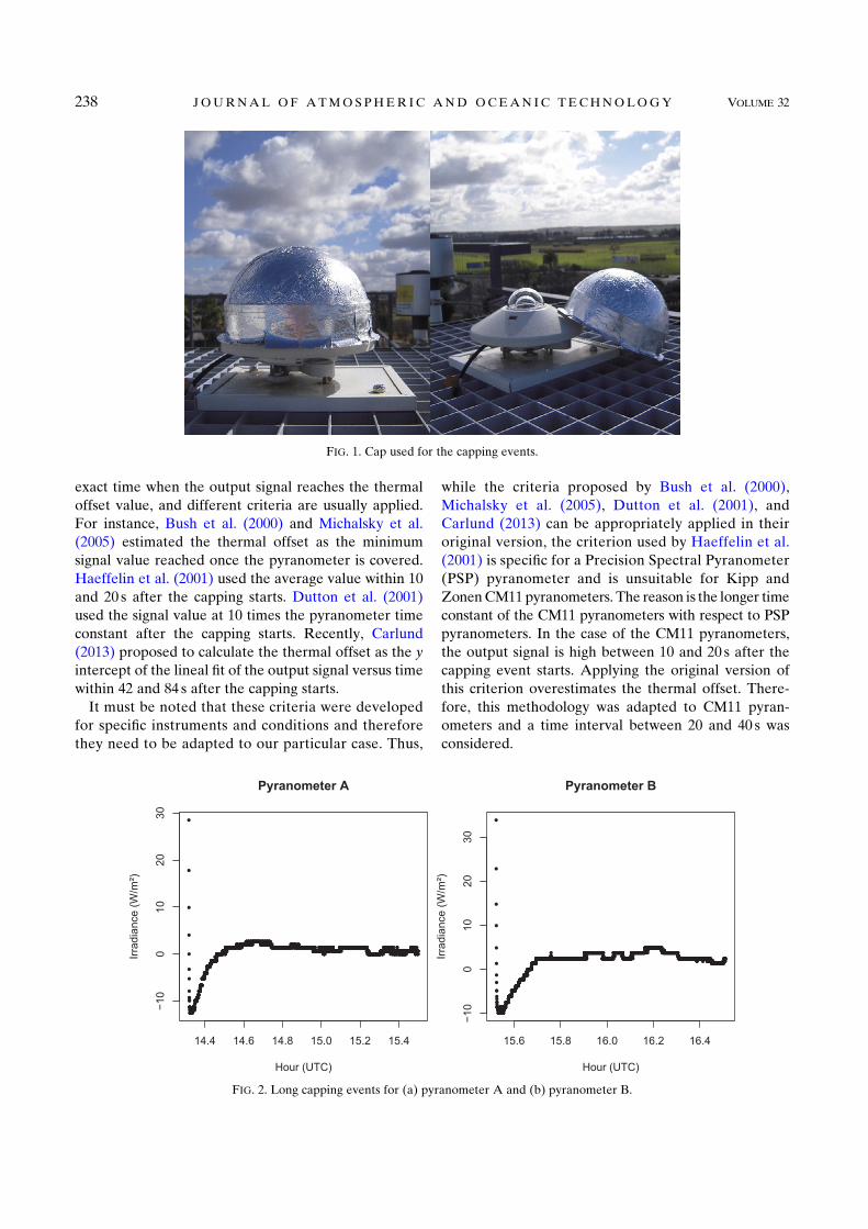
exact time when the output signal reaches the thermal

offset value, and different criteria are usually applied.

For instance, Bush et al. (2000) and Michalsky et al.

(2005) estimated the thermal offset as the minimum

signal value reached once the pyranometer is covered.

Haeffelin et al. (2001) used the average value within 10

and 20 s after the capping starts. Dutton et al. (2001)

used the signal value at 10 times the pyranometer time

constant after the capping starts. Recently, Carlund

(2013) proposed to calculate the thermal offset as the y

intercept of the lineal fit of the output signal versus time

within 42 and 84 s after the capping starts.

It must be noted that these criteria were developed

for specific instruments and conditions and therefore

they need to be adapted to our particular case. Thus,

while the criteria proposed by Bush et al. (2000),

Michalsky et al. (2005), Dutton et al. (2001), and

Carlund (2013) can be appropriately applied in their

original version, the criterion used by Haeffelin et al.

(2001) is specific for a Precision Spectral Pyranometer

(PSP) pyranometer and is unsuitable for Kipp and

ZonenCM11 pyranometers. The reason is the longer time

constant of the CM11 pyranometers with respect to PSP

pyranometers. In the case of the CM11 pyranometers,

the output signal is high between 10 and 20 s after the

capping event starts. Applying the original version of

this criterion overestimates the thermal offset. There-

fore, this methodology was adapted to CM11 pyran-

ometers and a time interval between 20 and 40 s was

considered.

FIG. 1. Cap used for the capping events.

FIG. 2. Long capping events for (a) pyranometer A and (b) pyranometer B.


The selection of a proper lasting time for the capping

events had to comply with different requirements. On

the one hand, it must be long enough to allow the ap-

plication of the described methodologies. The method-

ology that was more demanding was that from Carlund

(2013), which requires at least 84 s of capping. On the

other hand, the capping must be short enough not to

significantly modify the thermal balance between the

dome and the detector. To comply with both require-

ments, we decided to perform capping events lasting

1.5min. This is the minimum time needed to calculate the

thermal offset according to the different criteria described

above without significantly affecting the pyranometer

temperature imbalance.

Subsequently, numerous 1.5-min-lasting capping events

were conducted. The thermal offset of our two pyran-

ometers were measured one after another. The interval

between the two consecutive capping events was, at least,

2min in order to avoid memory effects. The irradiance

(global, diffuse, direct, and IR), wind speed, and ambient

temperature values ascribed to each capping event were

considered as those registered 2 s before capping the

pyranometer.

The thermal offset will be calculated by applying these

four different criteria under different environment

conditions and the results will be analyzed. Finally,

a suitable criterion will be chosen.

c. Analysis

Once the most suitable criterion for estimating the

thermal offset was selected, the values obtained for the

two pyranometers under different conditions were

studied in detail. Differences in the thermal offset be-

tween daytime and nighttime, under different cloud

conditions, and between pyranometers working in the

same conditions were analyzed and compared. Differ-

ences in thermal offset error between global and diffuse

measurements were also investigated.

The relationship between thermal offset and various

radiation and environmental variables have been

addressed in numerous studies (Bush et al. 2000;

Haeffelin et al. 2001; Dutton et al. 2001; Vignola et al.

2007; Ji and Tsay 2010). In particular, the ambient

temperature has been reported by many authors as

a main factor for the thermal offset (Bush et al. 2000;

Dutton et al. 2001; Haeffelin et al. 2001; Philipona 2002;

Ji and Tsay 2010). Additionally, the temperature Tp of

a collocated pyrgeometer is of special interest, since

some authors have indicated its high correlation with the

pyranometer temperature due to the similar design of

both instruments (Dutton et al. 2001; Ji and Tsay 2010).

Moreover, several authors have pointed out the re-

lationship between the thermal offset of a pyranometer

and the Net IR measured by a collocated pyrgeometer

(Dutton et al. 2001; Haeffelin et al. 2001). These mag-

nitudes are key factors in the local energy balance, which

affects the temperature of the pyranometer dome.

In addition, thermal offset dependences on the clear-

ness index kt and the diffuse fraction Kd were analyzed.

These ratios provide information about the relative at-

tenuation suffered by the radiation when crossing the at-

mosphere. These ratios are defined by the following

expressions:

kt 5Ig

ITOA

, (2a)

Kd 5IdIg, (2b)

respectively, where Ig, and Id are the global and diffuse

irradiance on a horizontal surface on the earth’s surface,

respectively, and ITOA represents the actual irradiance

on a horizontal surface at the top of the atmosphere,

which is calculated as follows:

ITOA 5 1370Wm22 E0 cos(u) , (3)

where E0 stands for the eccentricity correction due to

the earth–sun actual distance and u stands for the solar

zenith angle.

d. Schedule of measurements

To investigate the thermal offset of the two

pyranometers under different cloud and ambient tem-

perature conditions, measurements with different con-

figurations were performed. Table 1 summarizes the

main characteristics of the capping events conducted.

It provides information about the date, the cloud con-

dition, the variable measured by each pyranometer

(global or diffuse), the number of capping events for

each day of measurement, and the ranges of different

variables (ambient temperature, wind speed, net in-

frared irradiance, global solar, and diffuse solar irradi-

ance). The range refers to the interval of variation of

each variable corresponding to the capping events con-

ducted each day.

The variety of episodes allowed for studying several

aspects of the thermal offset effect. Thus, with the aim to

analyze the possible differences in the thermal offset

between the two pyranometers, both instruments mea-

sured the same variable (global or diffuse) during days

171, 172, 177, and 178. On the other hand, in order to

evaluate the main factors affecting the thermal offset,

each pyranometer measured the same variable (global or

diffuse irradiance) during days with different temperature,


wind speed, and cloud conditions. For example,

pyranometer A measured global irradiance during days

73, 87, 136, 171, 178, and 199 (Table 1). Additionally, in

order to study the possible differences in the thermal

offset values when the pyranometer measures global or

diffuse irradiance, pairs of consecutive days have been

used; one day the pyranometer measured global irradi-

ance, while the next day it measured diffuse irradiance.

For this comparison, consecutive days with similar

temperature, wind speed, and cloud conditions, such as

days 199 and 200, were selected. Finally, during some

days one pyranometer measured global irradiance,

while the other measured diffuse irradiance, with the

aim to have enough measurements of all the variables

used in the study.

4. Results and discussion

a. Comparison of criteria

The thermal offsets of the two pyranometers were

estimated following the original criteria proposed by

Bush et al. (2000), Dutton et al. (2001), and Carlund

(2013), and the Haeffelin et al. (2001) criterion was

adapted as described in section 3.

Figure 3 shows the thermal offset values obtained by

applying the four criteria to pyranometer A on an

overcast day and a clear day (days 136 and 199, re-

spectively). During both days pyranometer A measured

global irradiance. In general, the absolute differences

between different criteria are mostly under 1.5Wm22

on clear days, and nearly zero on cloudy days. In

particular, the results obtained by applying Bush and

Dutton’s criteria agree overall. In contrast, on clear

days, the adapted Haeffelin et al.’s criterion seems to

give slightly higher values. These results agree with the

paired t tests at a 95% confidence level performed be-

tween the two criteria. The tests indicate no statistically

significant differences between Bush et al.’s and Dutton

et al.’s criteria. On the other hand, Carlund’s and

Haeffellin et al.’s criteria show significant differences

with respect to any other criterion.

In this framework it is worth noting that no best crite-

rion can be established and that the decision must be

based on practical considerations. In this study, the Bush

et al. (2000) methodology was preferred, since it requires

no estimation of any characteristic of the pyranometer,

such as its time constant, which can be inaccurate or dif-

ficult to determine.

b. Experimental values of the thermal offset

Figure 4, top panels, shows the thermal offset obtained

by capping pyranometers A and B under different cloudTABLE1.Date,cloudcondition,variable

measured,andrangeofambienttemperature

(DTa),windspeed(D

w),Net

IR(D

Net

IR),global(D

I g)anddiffuse

(DI d)irradiance

duringthe

cappingeventsconductedeach

day.

Cappingevents

Date

14Mar2013

28Mar2013

16May2013

20Jun2013

21Jun2013

26Jun2013

27Jun2013

18Jul2013

19Jul2013

Dayofyear

73

87

136

171

172

177

178

199

200

Cloudcondition

Clear

Overcast

Overcast

Clear

Cirrostratus

Clear

Clear

Clear

Clear

DTa(8C)

108–148

148–158

168–14.58

168–308

188–308

288–368

258–358

208–368

208–378

Windspeed(m

s21)

1.4–3.4

2.8–4.9

4.5–7.6

1.2–3.8

1.7–4.5

0.6–1.6

1.2–3.2

0.9–3.3

0.5–4.4

DNetIR

(Wm

22)

2139,2113

253,215

247,228

2135,294

2123,281

2128,2107

2126,289

2126,286

2122,291

DI g

(Wm

22)

185,834

125,860

106,350

374,988

300,1016

577,958

422,886

259,990

303,971

DI d

(Wm

22)

40,66

160,494

106,350

59,87

138,475

116,176

116,204

85,118

72,126

PA

PB

PA

PB

PA

PB

PA

PB

PA

PB

PA

PB

PA

PB

PA

PB

PA

PB

Variab

lemeasured

Glo.

Dif.

Glo.

Dif.

Glo.

Dif.

Glo.

Glo.

Dif.

Dif.

Dif.

Dif.

Glo.

Glo.

Glo.

Dif.

Dif.

Glo.

No.ofcappingevents

12

12

10

10

13

13

20

19

16

15

66

88

15

15

14

14


conditions along with the corresponding nighttime

measurements. In spite of corresponding to the same

pyranometer model, significant differences between

pyranometers A and B are observed when they were

measured under the same environmental conditions

(days 171, 172, 177, and 178). The absolute thermal

offset of pyranometer A is usually higher than the

thermal offset of pyranometer B. This fact can be also

observed in Fig. 2. The larger differences, up to

3.48Wm22, occur when both pyranometers measure

global irradiance, while the differences decrease to

a mean value of 0.37Wm22 when they measure diffuse

irradiance. To statistically assess the significance of

these differences, two sample t tests were performed.

The test resulted in significant differences at a 95%

confidence level. This result indicates that the thermal

offset must be determined for each instrument in-

dividually, even if they correspond to the same manu-

facturer and model.

The thermal offset of pyranometer A (B) ranges from

219Wm22 (216Wm22) on a cloud-free hot day to

20.5Wm22 (10.6Wm22) on an overcast daywith amild

temperature. This decrease in the absolute value of the

thermal offset under cloudy conditions agrees with re-

sults obtained by other authors (Bush et al. 2000; Dutton

et al. 2001) who suggest it is due to the enhancement of

downward IR by clouds, heating the pyranometer dome

and reducing the dome-detector temperature difference.

Under certain atmospheric conditions, the temperature

of the dome can be higher than the temperature of the

detector, resulting in a positive offset (Bush et al. 2000;

Dutton et al. 2001). The thermal offset on clear days

(73, 171, 177–200) is notably lower at sunrise/sunset than

at noon. At sunrise and sunset, the diffuse fraction Kd is

higher because of the longer path traveled by the radi-

ation within the atmosphere. These results point out the

important effect on the thermal offset of both the

quantity and distribution of the radiation. Figure 4,

bottom panels, shows the normalized thermal offset

(divided by the irradiance) for daytime measurements.

These relative values range from 1% for irradiance

during cloudy days to over 15% for diffuse irradiance

during cloud-free days.

Figure 4, top panels, shows notable differences in the

thermal offset between daytime and nighttime (see, for

instance, days 199 and 200). This fact agrees with results

reported by several authors for other pyranometer

models and locations (Cess et al. 2000; Haeffelin et al.

2001; Philipona 2002; Ji and Tsay 2010). The nighttime

offset on different days ranges from 0 to 25Wm22. In

contrast, the daytime thermal offset can reach values

under 215Wm22. There are also notorious differences

in the variability. Thus, while the daytime thermal offset

under cloud-free conditions can vary up to 8Wm22,

during the corresponding nighttime the variability rarely

exceeds 2Wm22. These significant differences between

day and night advise against the common procedure of

using the averaged nighttime measurements as daytime

thermal offset.

It is worth noting the differences in thermal offset

between days with similar cloud cover, Net IR, and wind

speed but different temperature ranges, such as days 73

and 199 (see Table 1). Figure 4, top panels, shows that

lower ambient temperatures in day 73 result in lower

thermal offset for both pyranometers.

Days 199 and 200 show differences regarding mea-

suring global or diffuse radiation. These differences

have been evaluated, and values in the range from 0.61

to 5.86Wm22 for pyranometer A and from 0.56 to

3.74Wm22 for pyranometer B have been obtained.

Although these differences are lower than the values

obtained by Bush et al. (2000) for a PSP pyranometer

(about 8.5Wm22), these differences are significant, as

confirmed by a two-sample t test at a 95% confidence

level. This finding is counter to results obtained by

Philipona (2002) but agrees with Bush et al. (2000) and

Cess et al. (2000), who reported differences depending

on whether global or diffuse irradiance is measured.

This open issue emphasizes the need for studying dif-

ferent pyranometers’ families and models.

c. Relationship with some radiative variables

The relationship of the experimental thermal offset

with some radiative and environment variables was

FIG. 3. Thermal offset obtained with different methodologies for

pyranometer A when measuring global irradiance on an overcast

day (136) and a clear day (199).


studied. It must be noted that, since the essayed vari-

ables are not independent, they are considered in-

dividually in the search of a good fit. Figures 5a–f show

the daytime thermal offset (gray points) versus the

ambient temperature, the clearness index, the diffuse

and direct fractions, the Net IR irradiance, the tem-

perature in a collocated pyrgeometer, and the wind

speed for pyranometer A. Figures 5e,f show also the

nighttime measurements (black points). A clear re-

lationship with ambient and pyrgeometer tempera-

tures and with radiation is found, in agreement with

results reported for other pyranometer models

(Gulbrandsen 1978; Wardle et al. 1996; Ji and Tsay

2010). Thermal offset decreases when ambient tem-

perature (Fig. 5a), pyranometer temperature (Fig. 5f),

and clearness index (Figs. 5c) increase. The diffuse

fraction of the radiation plays an important role.

Hence, the thermal offset increases when Kd increases

(Fig. 5d). The analysis of the Net IR dependence shows

similar thermal offset values for cloudy conditions

(black points with higher Net IR) and nighttime (gray

points) but large differences with daytime values

(black points with lower Net IR) (Fig. 5e). A similar

result can be observed in the thermal offset versus

pyrgeometer temperature relationship (Fig. 5f).

To assess these relationships, least squares regressions

between the thermal offset of pyranometer A and each

independent variable have been constructed. For this

aim the dataset has been split into two subsets: 75% (84

data) for the fitting and the remaining independent 25%

(28 data) for the validation. The fittings are moderately

good with the coefficient of correlations ranging from

0.64 for the wind to 0.84 for Kd. When these fittings are

applied to the independent set, root-mean-square errors

(RMSE) under 3.8Wm22 are obtained, showing

a moderate predictive skill.

FIG. 4. Nighttime and daytime thermal offset obtained for (top left) pyranometer A and (top right) pyranometer B

and daytime thermal normalized (divided by the irradiance) offset for (bottom left) pyranometer A and (bottom

right) pyranometer B.


Figures 5a–f show a complex relationship of the

thermal offset with the ambient temperature, the radi-

ation magnitude, and its distribution. Higher thermal

offset takes place on clear days around noon, when

irradiance, but not the ambient temperature, reaches its

maximum value. The simultaneous dependence on

temperature and irradiance can be clearly seen in

Figs. 6a, where the thermal offset of each pyranometer

FIG. 5. Pyranometer A thermal offset vs (a) ambient temperature Ta, ( b) wind speed, (c) clearness index kt,

(d) diffuse fraction kd, (e) Net IR, and (f) pyrgeometer temperature Tp.


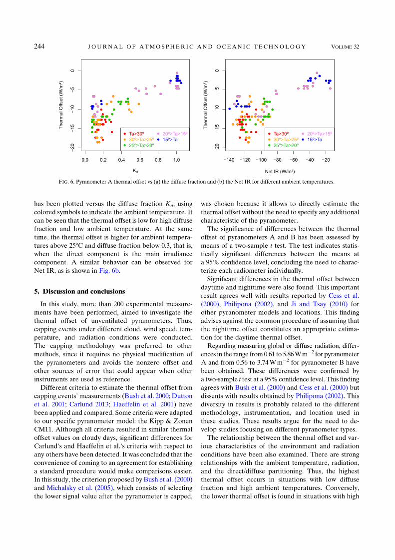
has been plotted versus the diffuse fraction Kd, using

colored symbols to indicate the ambient temperature. It

can be seen that the thermal offset is low for high diffuse

fraction and low ambient temperature. At the same

time, the thermal offset is higher for ambient tempera-

tures above 258C and diffuse fraction below 0.3, that is,

when the direct component is the main irradiance

component. A similar behavior can be observed for

Net IR, as is shown in Fig. 6b.

5. Discussion and conclusions

In this study, more than 200 experimental measure-

ments have been performed, aimed to investigate the

thermal offset of unventilated pyranometers. Thus,

capping events under different cloud, wind speed, tem-

perature, and radiation conditions were conducted.

The capping methodology was preferred to other

methods, since it requires no physical modification of

the pyranometers and avoids the nonzero offset and

other sources of error that could appear when other

instruments are used as reference.

Different criteria to estimate the thermal offset from

capping events’ measurements (Bush et al. 2000; Dutton

et al. 2001; Carlund 2013; Haeffelin et al. 2001) have

been applied and compared. Some criteria were adapted

to our specific pyranometer model: the Kipp & Zonen

CM11. Although all criteria resulted in similar thermal

offset values on cloudy days, significant differences for

Carlund’s and Haeffelin et al.’s criteria with respect to

any others have been detected. It was concluded that the

convenience of coming to an agreement for establishing

a standard procedure would make comparisons easier.

In this study, the criterion proposed by Bush et al. (2000)

and Michalsky et al. (2005), which consists of selecting

the lower signal value after the pyranometer is capped,

was chosen because it allows to directly estimate the

thermal offset without the need to specify any additional

characteristic of the pyranometer.

The significance of differences between the thermal

offset of pyranometers A and B has been assessed by

means of a two-sample t test. The test indicates statis-

tically significant differences between the means at

a 95% confidence level, concluding the need to charac-

terize each radiometer individually.

Significant differences in the thermal offset between

daytime and nighttime were also found. This important

result agrees well with results reported by Cess et al.

(2000), Philipona (2002), and Ji and Tsay (2010) for

other pyranometer models and locations. This finding

advises against the common procedure of assuming that

the nighttime offset constitutes an appropriate estima-

tion for the daytime thermal offset.

Regarding measuring global or diffuse radiation, differ-

ences in the range from0.61 to 5.86Wm22 for pyranometer

A and from 0.56 to 3.74Wm22 for pyranometer B have

been obtained. These differences were confirmed by

a two-sample t test at a 95% confidence level. This finding

agrees with Bush et al. (2000) and Cess et al. (2000) but

dissents with results obtained by Philipona (2002). This

diversity in results is probably related to the different

methodology, instrumentation, and location used in

these studies. These results argue for the need to de-

velop studies focusing on different pyranometer types.

The relationship between the thermal offset and var-

ious characteristics of the environment and radiation

conditions have been also examined. There are strong

relationships with the ambient temperature, radiation,

and the direct/diffuse partitioning. Thus, the highest

thermal offset occurs in situations with low diffuse

fraction and high ambient temperatures. Conversely,

the lower thermal offset is found in situations with high

FIG. 6. Pyranometer A thermal offset vs (a) the diffuse fraction and (b) the Net IR for different ambient temperatures.


diffuse fraction and low ambient temperatures. The

corresponding least squares regression between the

thermal offset and each independent variable has been

constructed, showing moderate predictive skill and the

relationship withKd, the one with the best performance,

with a correlation coefficient of about 0.84.

This work aims to contribute to better knowledge of

the pyranometer thermal offset error, in particular for

the widely used Kipp & Zonen CM11. It is worth

noting that, due to the difference in atmospheric con-

ditions, the thermal offset of a particular pyranometer

at one location may be different from the offset mea-

sured at another location. This fact emphasizes the

importance of performing on-site measurements of the

thermal offset. However, although our results apply

solely to our specific instruments at our particular lo-

cation, the methodology and comparisons described in

this paper can be used to develop similar analysis at

other locations, with other instruments and environ-

mental conditions. In fact, the complete knowledge of the

thermal offset issue will be achieved by a collection of

studies that analyze specific instruments at particular lo-

cations. This study also suggests directions for future re-

search concerning the development of correction models

for the thermal offset.

Acknowledgments. This study was partially supported

by the research project CGL2011-29921-C02-01 granted

by the Ministerio de Economía y Competitividad fromSpain and by Ayuda a Grupos GR10131 granted byGobierno de Extremadura and Fondo Social Europeo.Guadalupe SanchezHernandez thanks theMinisterio deEconomía y Competitividad for the predoctoral FPIgrant. The Centra Territorial de Extremadura de laAgencia Estatal de Meteorología (AEMET) at Badajozand the ‘‘El Arenosillo’’ Atmospheric Sounding Station

(ESAt) of the National Institute for Aerospace Tech-

nology (INTA) in Huelva provided suitable facilities for

the pyranometer comparisons.

REFERENCES

Bush, B. C., F. P. J. Valero, and A. S. Simpson, 2000: Charac-

terization of thermal effects in pyranometers: A data cor-

rection algorithm for improved measurement of surface

insolation. J. Atmos. Oceanic Technol., 17, 165–175,

doi:10.1175/1520-0426(2000)017,0165:COTEIP.2.0.CO;2.

Carlund, T., 2013: Baltic region pyrheliometer comparison 2012: 21

May–1 June 2012, Norrköping, Sweden, World Meteorologi-cal Organization Rep., Instruments and Observing MethodsRep. 112, 40 pp.

Cess, R. D., T. Qian, andM. Sun, 2000: Consistency tests applied to

the measurement of total, direct, and diffuse shortwave radi-

ation at the surface. J. Geophys. Res., 105, 24 881–24 887,

doi:10.1029/2000JD900402.

Dutton, E. G., J. J. Michalsky, T. Stoffel, B. W. Forgan, J. Hickey,

D. W. Nelson, T. L. Alberta, and I. Reda, 2001: Measurement

of broadband diffuse solar irradiance using current commer-

cial instrumentation with a correction for thermal offset er-

rors. J. Atmos. Oceanic Technol., 18, 297–314, doi:10.1175/

1520-0426(2001)018,0297:MOBDSI.2.0.CO;2.

Garratt, J. R., 1994: Incoming shortwave fluxes at the surface—

A comparison of GCM results with observations. J. Cli-

mate, 7, 72–80, doi:10.1175/1520-0442(1994)007,0072:

ISFATS.2.0.CO;2.

Gulbrandsen, A., 1978: On the use of pyranometers in the study of

spectral solar radiation and atmospheric aerosols. J. Appl.

Meteor., 17, 899–904, doi:10.1175/1520-0450(1978)017,0899:

OTUOPI.2.0.CO;2.

Haeffelin,M., S. Kato,A.M. Smith, C. K.Rutledge, T. P. Charlock,

and J. R. Mahan, 2001: Determination of the thermal offset of

the Eppley precision spectral pyranometer. Appl. Opt., 40,

472–484, doi:10.1364/AO.40.000472.

Halthore, R. N., S. Nemesure, S. E. Schwartz, D. G. Irme, A. Berk,

E. G. Dutton, and M. H. Bergin, 1998: Models overestimate

diffuse clear-sky surface irradiance: A case for excess atmo-

spheric absorption. Geophys. Res. Lett., 25, 3591–3594,

doi:10.1029/98GL52809.

Ji, Q., and S.-C. Tsay, 2010:A novel nonintrusivemethod to resolve

the thermal dome effect of pyranometers: Instrumentation

and observational basis. J. Geophys. Res., 115, D00K21,

doi:10.1029/2009JD013483.

Kato, S., T. P. Ackerman, E. E. Clothiaux, J. H. Mather, G. G.

Mace, M. L. Wesely, F. Murcray, and J. Michalsky, 1997:

Uncertainties in modeled and measured clear-sky surface

shortwave irradiance. J. Geophys. Res., 102, 25 881–25 898,

doi:10.1029/97JD01841.

Kipp and Zonen, 2000: Instruction manual for CM11 and

CM14 pyranometer/albedometer, version 0805, 62 pp.

[Available online at http://www.kippzonen.com/Download/

48/CM-11-Pyranometer-CM-14-Albedometer-Manual.]

——, 2003: Instruction manual for CG1 and CG2 pyrgeo-

meter and net pyrgeometer, version 0204, 63 pp. [Avail-

able online at http://www.kippzonen.com/Download/31/

CG-1-CG-2-Pyrgeometers-Manual.]

Long, C. N., K. Younkin, K. L. Gaustad, and J. A. Augustine, 2003:

An improvement daylight correction for IR loss in ARM

diffuse SW measurements. Proceedings of the Thirteenth At-

mospheric Radiation Measurement Science Team Meeting,

D. A. Carrothers, Ed., U.S. Department of Energy, 1–8.

Michalsky, J. J., and Coauthors, 2005: Toward the development of

a diffuse horizontal shortwave irradiance working standard.

J. Geophys. Res., 110, D06107, doi:10.1029/2004JD005265.

Pachauri, R. K., andA.Reisinger, Eds., 2007:Climate Change 2007:

Synthesis Report. Cambridge University Press, 104 pp.

Patsalides, M., and Coauthors, 2007: The effect of solar irradiance

on the power quality behaviour of grid connected photovoltaic

systems. Proc. Int. Conf. on Renewable Energy and Power

Quality (ICREPQ’07), Seville, Spain, EA4EPQ, 284. [Avail-

able online at http://www.icrepq.com/icrepq07/284-patsalides.

pdf.]

——, A. Stavrou, V. Efthymiou, and G. E. Georghiou, 2012: To-

wards the establishment of maximum PV generation limits

due to power quality constraints. Int. J. Electr. Power Energy

Syst., 42, 285–298, doi:10.1016/j.ijepes.2012.03.043.

Philipona, R., 2002: Underestimation of solar global and diffuse

radiation measured at Earth’s surface. J. Geophys. Res., 107,

4654, doi:10.1029/2002JD002396.


Reda, I., T. Stoffel, andD.Myers, 2003: Amethod to calibrate a solar

pyranometer for measuring reference diffuse irradiance. Sol.

Energy, 74, 103–112, doi:10.1016/S0038-092X(03)00124-5.

Smith, A. M., 1999: Prediction and measurement of thermal ex-

change within pyranometers. M.S. thesis, Dept. of Mechanical

Engineering, Virginia Polytechnic Institute and State Uni-

versity, 64 pp.

Valero, F. P., and B. C. Bush, 1999: Measured and calculated clear-

sky solar radiative fluxes during the SubsonicAircraft Contrail

and Cloud Effects Special Study (SUCCESS). J. Geophys.

Res., 104, 27 387–27 398, doi:10.1029/1999JD900947.

Vignola, F., C.N.Long, and I.Reda, 2007: Evaluation of methods to

correct for IR loss in Eppley PSP diffuse measurements.

Optical Modeling and Measurements for Solar Energy Sys-

tems, D. R. Myers, Ed., International Society for Optical En-

gineering (SPIE Proceedings, Vol. 6652), 66520A, doi:10.1117/

12.73447.

——,——, and——, 2008:Modeling IR radiative loss fromEppley

PSP Pyranometers. Optical Modeling and Measurements for

Solar Energy Systems II, B. K. Tsai, Ed., International Society

for Optical Engineering (SPIE Proceedings, Vol. 7046),

70460E, doi:10.1117/12.796457.

——, ——, and ——, 2009: Testing a model of IR radiative losses.

Optical Modeling and Measurements for Solar Energy Sys-

tems III, B. K. Tsai, Ed., International Society for Optical

Engineering (SPIE Proceedings, Vol. 7410), 741003,

doi:10.1117/12.826325.

Wardle, D. I., and Coauthors, 1996: Improved measurements of

solar irradiance by means of detailed pyranometer charac-

terisation. Int. Energy Agency Rep. IEA-SHCP-9C-2, 364 pp.

Wild, M., 2005: Solar radiation budgets in atmospheric model in-

tercomparison from a surface perspective.Geophys. Res. Lett.,

32, L07704, doi:10.1029/2005GL022421.

——, 2009: Global dimming and brightening: a review. J. Geophys.

Res., 114, D00D16, doi:10.1029/2008JD011470.

——,A. Ohmura, H. Gilgen, E. Roeckner, M. Giorgetta, and J. J.

Morcrette, 1998: The disposition of radiative energy in the

global climate system: GCM-calculated versus observa-

tional estimates. Climate Dyn., 14, 853–886, doi:10.1007/

s003820050260.

——, and Coauthors, 2005: From dimming to brightening: Decadal

changes in surface solar radiation. Science, 308, 847–850,

doi:10.1126/science.1103215.

——, D. Folini, C. Schar, N. Loeb, E. G. Dutton, and G. Konig-

Langlo, 2013: The global energy balance from a surface

perspective. Climate Dyn., 40, 3107–3134, doi:10.1007/

s00382-012-1569-8.

WMO, 2008: Guide to meteorological instruments and methods of

observation. 7th ed. No. 8, Secretariat of the World Meteo-

rological Organization, 681 pp.


3.2. ARTICULO 1 53

3.2.4. Informe del Director de la Tesis Doctoral

El artıculo ”Pyranometer thermal offset: Measurement and analysis”, fue

publicado en la revista Journal of Atmospheric and Oceanic Technology en el ano

2015, teniendo la revista un factor de impacto de 2.159 y estando incluida en el

primer cuartil (Q1, ranking 2 de 14 revistas) dentro de la categorıa “Engineering,

Ocean”.

La participacion de la doctoranda Dna. Guadalupe Sanchez Hernandez en este

artıculo ha sido muy elevada y diversa, colaborando muy activamente en todas las

etapas desarrolladas para la obtencion del artıculo, desde la concepcion de la idea

original hasta la propuesta, diseno y toma de medidas, el analisis de resultados y

la elaboracion del manuscrito. Merece la pena destacar el gran trabajo y esfuerzo

que ha dedicado a la realizacion de experimentos de tapado, lo que ha exigido

creatividad e iniciativa para resolver los problemas que surgen al implementar una

metodologıa por primera vez.

Todas estas las tareas han sido desarrolladas por la doctoranda bajo mi direccion

y supervision, pudiendo dar fe de que todo lo aquı expuesto es verıdico.

Fdo.: El Director de la Tesis Doctoral

Por otra parte, D. Antonio Serrano Perez, Dna. Marıa Luisa Cancillo Fernandez

y D. Jose Agustın Garcıa Garcıa, coautores de este artıculo, afirman mediante este

escrito que han colaborado en este artıculo pero que este forma parte ıntegra de la

Tesis Doctoral de Dna. Guadalupe Sanchez Hernandez y que no va a ser utilizado

por ellos como parte de sus respectivas tesis doctorales.

Dna. Mª Luisa Cancillo Fernandez D. Jose Agustın Garcıa Garcıa


3.3. Artıculo 2


Tıtulo: Correcting daytime thermal offset in unventilated pyranometers

Autores: Antonio Serranoa

Guadalupe Sancheza

Mª Luisa Cancilloa



Volumen: 32 Paginas: 2088 - 2099 Ano de publicacion: 2015

doi: 10.1175/JTECH-D-15-0058.1


El principal objetivo de este trabajo es la propuesta de modelos empıricos para

la correccion del cero termico en las medidas diurnas de irradiancia difusa y global

en piranometros sin ventilacion artificial. En este trabajo se han analizado tanto

modelos de una sola variable como distintas combinaciones lineales de varias de

ellas. Asimismo, se ha analizado la posibilidad de utilizar modelos desarrollados a

partir de datos nocturnos para predecir los valores de cero termico diurno. Ademas,

la utilizacion en este estudio de dos piranometros del mismo modelo ha permitido

analizar la generalidad de los coeficientes de los modelos finalmente propuestos.

Para este trabajo se han utilizado los valores de cero termico obtenidos me-

diante la metodologıa de tapados descritos en el Artıculo 1. Estas medidas fueron

tomadas bajo una gran variedad de condiciones atmosfericas lo que garantiza la

representatividad del estudio.

Los modelos empıricos propuestos en este trabajo incluyen diversas variables

meteorologicas que influyen en la diferencia de temperatura entre el sensor y la

cupula del piranometro, que es, finalmente, el origen del cero termico. Las variables

ensayadas han sido la temperatura ambiente, la velocidad de viento, la humedad

relativa, la radiacion infrarroja descendente, la radiacion infrarroja neta, la tempe-

ratura de un pirgeometro cercano, el ındice de claridad y la fraccion de irradiancia

difusa. Estas magnitudes presentan ademas la ventaja de ser frecuentemente

medidas en las estaciones radiometricas.

Entre los modelos de una variable propuestos en este estudio destacan aquellos

3.3. ARTICULO 2 55

cuya variable independiente es la fraccion de irradiancia difusa (kd) o la temperatura

de un pirgeometro instalado junto al piranometro (Tp). El primero de estos modelos,

denominado Modelo kd es este artıculo, destaca por permitir la correccion del

cero termico a partir de las propias medidas de irradiancia global y difusa, sin

necesidad de instrumentacion adicional. Los modelos de una variable han sido

analizados tambien para valores nocturnos de thermal offset. Los valores del RMSE

obtenidos al aplicar los coeficientes nocturnos a los datos diurnos son superiores a

7.3 W/m2 para todos los modelos. Esto indica que la aplicacion de los modelos obte-

nidos a partir de datos nocturnos solo corrigen parcialmente el thermal offset diurno.

Para la propuesta de modelos con varias variables se partio de un conjunto inicial

de 223 modelos que surge de la combinacion de las todas variables consideradas en

modelos de entre dos y ocho variables. Sin embargo, algunas de estas combinaciones

presentaban una elevada autocorrelacion entre sus variables que podrıa afectar a

la estabilidad de los coeficientes de ajuste. Para detectar y descartar los modelos

en los que aparecıa autorcorrelacion se recurrio al uso de herramientas estadısticas

adecuadas.

Con el analisis estadıstico de la autocorrelacion el numero de modelos se redujo

a 46 de los cuales finalmente se analizaron los diez con el mayor valor del coeficiente

de determinacion. Entre estas diez combinaciones lineales finalmente propuestas

destaca la formada por kd y tp y la formada por kd e IR. Ademas de las medidas

de irradiancia global y difusa, estos modelos requieren de las medidas simultaneas

de un pirgeometro. No obstante, las otras combinaciones tambien muestran buenos

resultados, lo que permite seleccionar el modelo mas adecuado en funcion de las

variables disponibles.

Aunque el uso de los piranometros CMP11 utilizado en este estudio esta muy

extendido, debemos reconocer que los resultados obtenidos en este trabajo son

especıficos para este instrumento y para nuestra localizacion. Tanto las dependencias

funcionales como los coeficientes empıricos aquı mostrados podrıan variar tanto con

el modelo de piranometro como con la localizacion. Es por ello que resulta de gran

interes evaluar la generalidad de los modelos propuestos en este trabajo con otros

modelos de piranometros y/o en otras localizaciones.


Correcting Daytime Thermal Offset in Unventilated Pyranometers

A. SERRANO, G. SANCHEZ, AND M. L. CANCILLO

Department of Physics, University of Extremadura, Badajoz, Spain

(Manuscript received 25 March 2015, in final form 21 July 2015)

ABSTRACT

A main source of error in solar radiation measurements is the thermal offset inherent to pyranometers.

Despite acknowledgment of its importance, its correction has been widely ignored for several decades. This

neglect may have caused a generalized underestimation in solar radiation measurements. This study focuses on

the correction of this error in solar irradiance measurements. For this aim a plethora of correction models built

as a linear combination of several environmental variables related to the ambient temperature and to the in-

coming radiation were proposed. The models are fitted to experimental measurements obtained during capping

events and, finally, their performance is evaluated and compared. The main results indicate that models with

only one independent variablemoderately correct the thermal offset error. These simplemodels are useful when

no additional instrumentation other than the pyranometer is available. On the other hand, the more complex

models show the best performance, with a coefficient of determination R2 over 0.8, an RMSE under 2Wm22,

and an absolute value of mean bias error (MBE) under 0.5Wm22. Additionally, these models are used to study

the differences between nighttime and daytime correction, revealing the unsuitability of using nighttime-fitted

models to correct the daytime thermal offset. The general validity of the models is tested by their application to

two different pyranometers. Results indicate that, whereas the factors involved in the best-performing models

are the same, the values of the loading coefficients differ and therefore must be specifically calculated for each

pyranometer.

1. Introduction

In recent years, scientific research and emerging solar

energy technologies demand an increase in the accuracy

of solar radiationmeasurements. Thus, some studies have

shown the dependence of climatic results on the mea-

suring methodology used and on the quality of radiation

measurements (Wang et al. 2013). Equally important is

the role played by high-quality measurements of the ra-

diation income at the earth’s surface for the use of solar

radiation as a renewable energy. The vertiginous increase

of energy demand requires improving both quantity and

quality of solar systems. The design of a solar system suit-

able for a certain location depends highly on the charac-

teristics of the local solar radiation field, where the

partitioning of direct/diffuse radiation is of particular im-

portance (Patsalides et al. 2007, 2012).

High-quality radiation values require identification and

correction of themain errors in pyranometermeasurements.

One of the sources of uncertainty first detected in solid

black pyranometers was the thermal offset. This error

is caused by the temperature difference between the

dome of the pyranometer and its detector, which produces

a spurious signal superimposed on the output signal

(Drummond and Roche 1965; Gulbrandsen 1978). In most

cases, the detector has a temperature higher than the

dome, producing a negative signal and, as a result, an un-

derestimation of the radiation. This signal has been quan-

tified to be between230 and25Wm22 depending on the

instrument design and environmental conditions (Reda

et al. 2003; Ji and Tsay 2010). Additionally, several studies

have shown notable differences between thermal offsets

measured at nighttime or daytime, under cloud or clear

conditions, and with high or low temperatures (Bush et al.

2000; Haeffelin et al. 2001; Dutton et al. 2001; Ji and Tsay

2010; Sánchez et al. 2015). Despite having been widely dis-

cussed, this error has been ignored for several decades.

Philipona (2002) estimated that this neglect may have pro-

duced an underestimation between 3% and 8% in solar

radiation measurements. However, the process is affected

by various environmental factors that make it difficult to

propose a thermal offset correction valid for all instrument

designs, locations, and environments (Bush et al. 2000).

Corresponding author address: Antonio Serrano, Department of

Physics, University of Extremadura, Avda. de Elvas s/n, 06071

Badajoz, Spain.

E-mail: [email protected]


DOI: 10.1175/JTECH-D-15-0058.1

� 2015 American Meteorological Society

Nevertheless, different approaches to correct this

error have been proposed. Some corrections focus on

the temperature difference between the dome and the

detector (Bush et al. 2000; Haeffelin et al. 2001) or on

related magnitudes, such as the pressure of the air

trapped between the outer and the inner domes (Ji and

Tsay 2010). The popular model developed by Dutton

et al. (2001) relies on the dome-detector temperature

difference and includes an additional term that re-

lates the thermal offset with the net infrared (IR) ir-

radiance measured by a collocated pyrgeometer. A

main limitation of this model appears for an in-

homogeneous radiation field, when the temperature

measured by the pyrgeometer may not be representa-

tive (Smith 1999). Additionally, nowadays, the great

majority of pyranometers lack temperature and pres-

sure detectors, and their installation can disturb the

measurements by interfering with the incoming radia-

tion. Therefore, other correction approaches need to

be used.

Dutton et al. (2001) showed that, under cloudy con-

ditions, the net IR term of their model could be used

alone to correct the thermal offset of solar diffuse ra-

diation measured by Eppley Precision Spectral Pyr-

anometers (PSPs). However, this approach is not

suitable for other conditions and other pyranometer

types, such as the widely used unventilated Kipp &

Zonen CM11 (Dutton et al. 2001; Carlund 2013).

Therefore, other authors have attempted to correct the

thermal offset using different methodologies and ten-

tative relationships, mainly based on ambient temper-

ature, relative humidity, and wind velocity (Vignola

et al. 2007, 2008, 2009). However, these relationships

have been tested only under very specific conditions

and instruments, and no thorough comparison has been

conducted yet.

The main objective of this paper is to propose models

for correcting the daytime pyranometer thermal offset

error. Toward this aim, capping events were conducted

to measure the daytime thermal offset of two unventilated

CM11 pyranometers under different cloud conditions,

ambient temperature, solar elevation, and operational

configuration (measuring global or diffuse solar radia-

tion). Simultaneously, radiative and environmental

magnitudes such as global and diffuse solar irradiance,

ambient temperature, downward total and net terres-

trial IR irradiance, temperature of the pyrgeometer,

wind speed, and relative humidity were measured.

Different correction models using these factors have

been proposed and compared. Some of these models

have been fitted using daytime or nighttime data in

order to investigate their possible differences. Addi-

tionally, the performance of the models when applied

to two different pyranometers was compared so as to

assess their possible wider applicability.

2. Data

a. Instrumentation

This empirical study is based on measurements of

global and diffuse solar irradiance, ambient tempera-

ture, downward total and net terrestrial infrared irradi-

ances, and detector temperature of a pyrgeometer

registered at the main radiometric station operated by

the research group Atmosphere, Climate and Radia-

tion in Extremadura (AIRE) of the University of

Extremadura. This station is placed on the roof of the

Physics Building at the university campus in Badajoz,

Spain (38.98N; 7.018W; 199m MSL). It includes a range

of radiometric instrumentation and benefits from an

open horizon, which guarantees the reliability of the

measurements.

Global and diffuse solar irradiance were measured by

two CM11 pyranometers with serial numbers 068948

and 027784, manufactured by Kipp & Zonen (pyran-

ometer A and pyranometer B, respectively). The CM11

model complies with International Organization for

Standardization (ISO) 9060 criteria for an ISO second-

ary standard pyranometer being classified as ‘‘high

quality’’ by WMO (1996). It guarantees a directional

error lower than 10Wm22 for zenith angles up to 808and a 1000Wm22 radiation beam (Kipp&Zonen 2000).

In addition to the original calibration performed by the

manufacturer, both pyranometers participated in two

intercomparison campaigns hosted by the Spanish State

Meteorological Agency [Agencia Estatal de Meteor-

ología (AEMET)] in Badajoz in April 2013 and by the

National Institute for Aerospace Technology [Instituto

Nacional de Técnica Aeroespacial (INTA)] in its At-

mospheric Sounding Station ‘‘ElArenosillo,’’ Huelva, in

June 2013. In these campaigns the two pyranometers

benefited from their comparison to two well-conditioned

and recently calibrated Kipp and Zonen CM21 pyran-

ometers with serial numbers 070122 and 041219, respec-

tively. The calibration factors obtained in both campaigns

are in good agreement with the values provided by the

manufacturer, showing relative differences under 0.5%

and therefore ensuring the temporal stability of the

pyranometers.

Diffuse solar irradiance measurements were ob-

tained by shading the pyranometer detector by a ball

that moves in synchronization with the sun motion so as

to continuously block the direct radiation. The pyran-

ometer and the shading ball were installed on the sun

tracker model SOLYS2 manufactured by Kipp &

Zonen (2008).

NOVEMBER 2015 S ERRANO ET AL . 2089

The temperature of the ambient air at the station was

monitored by a fast response temperature probe (model

PS-2135) connected to a PASCO GLX datalogger. The

temperature probe has a precision of 0.18C (PASCO

2014). It was shadowed and ventilated in order to guar-

antee the reliability of its measurements. The probe was

installed next to the pyranometers, being representative

of the air temperature at the station.

The radiometric station also includes a Kipp &Zonen

CG1 pyrgeometer for measuring downward atmo-

spheric infrared irradiance. In fact, it measures the net

radiation (NetIR), defined as the difference between the

downward infrared radiation emitted from the atmo-

sphere and the upward irradiance of the detector. To

take the emission of the detector into account, the in-

ternal temperature (Tp) is also registered. Thus, the total

downward atmospheric infrared irradiance (IR) is de-

rived as follows:

IR5NetIR1sT4p , (1)

where s is the Stefan–Boltzmann constant. The CG1

pyrgeometer has been designed to provide highly reliable

and accurate measurements of atmospheric infrared ra-

diation. It guarantees measurements with an error lower

than 20Wm22 and a zero offset lower than 2Wm22,

even under changing temperature conditions of 5Kh21

(Kipp & Zonen 2003). It is also very stable in time, with

the change in sensitivity lower than 1%yr–1. It has been

calibrated by Kipp & Zonen using the CG1 FT002 pyr-

geometer as a reference, resulting in a sensitivity error of

5% under conditions of a temperature of 208C and an

irradiance of 140Wm22 (Kipp & Zonen 2003).

All these data were recorded every minute except for

solar irradiance, measured by the pyranometers, which

was acquired every second in order to allow for accu-

rate determination of the thermal offset during the

capping events.

Additionally, wind speed and relative humidity were

monitored every 10min at a nearby meteorological

station located 400m away from our radiometric station.

This station belongs to AEMET and follows WMO

standard protocols and procedures for calibration and

measurement. Wind speed is measured by a Thies

Compact anemometer with serial number 4.3159.00.150.

The relative humidity is measured by a Thies Compact

sensor model 1.1025.55.700 with 0.18 resolution and 62%

accuracy. This sensor operates inside a Stevenson wooden

louver to prevent from heating by direct radiation.

b. Capping events

For the present study, a specific campaign was per-

formed consisting of determining the daytime thermal

offset by capping the pyranometers. The capping events

were conducted during 9 days between March and July

2013 (days of the year 73, 87, 136, 171, 172, 177, 178, 199,

and 200). These particular days were selected so as to

cover a wide range of cloud cover, temperature, wind,

and radiation conditions. All environmental variables

listed above were measured concurrently with these

capping events.

The capping methodology relies on obtaining the

thermal offset value analyzing the time evolution of the

output signal of the pyranometer once its detector is

suddenly capped. This technique has been widely applied

to different pyranometers (Bush et al. 2000; Dutton et al.

2001; Haeffelin et al. 2001; Michalsky et al. 2005; Carlund

2013). The reliability of this methodology has been

proved by Bush et al. (2000) and Haeffelin et al. (2001)

comparing its results with the difference of temperature

between the dome and the detector, which is the main

cause of the thermal offset. This methodology presents

the advantage of being nonintrusive since there is no need

to attach thermometers neither to the detector nor to the

dome, avoiding interfering with the incoming radiation

and therefore affecting the measurements. In the current

study, following the criteria suggested by Bush et al.

(2000) andMichalsky et al. (2005), the thermal offset was

obtained as the minimum value reached by the signal

once the pyranometer detector is capped. For a clear

identification of the minimum, the signal was recorded

every 1 s, and each capping event conducted in this study

took 1.5min. Figure 1 clearly illustrates the identification

of the thermal offset in a long capping event. The mea-

surements registered during the capping events showed

that, for our Kipp & Zonen CM11 pyranometers, this

minimum was reached about 25–35 s after the detector

was capped, and then the output signal remains constant

for about 20 s before starting to increase. For CM11

pyranometers, 1.5min is long enough to detect the re-

action of the detector and identify theminimum but short

enough to prevent significant changes in the dome tem-

perature or in the environmental conditions.

To obtain reliable estimations of the thermal offset by

using the capping methodology, a specific cap of poly-

styrene was built. This cap was designed to cover the

detector and dome while allowing for air circulation

around the pyranometer. The inside and outside of the

cap were covered with a reflective material. The cap was

maintained shadowed and refrigerated before each

capping event in order tominimize the IR exchange with

the domes. Further details about the capping events

conducted and the estimation of the thermal offset can

be found in Sanchez et al. (2015).

A total of 114 capping events with pyranometer A and

100 with pyranometer B were conducted; all of them


with a solar zenith angle lower than 808. In each capping

event, an estimate of the thermal offset was obtained.

Additionally, the most representative measurements

of the environmental variables available for each cap-

ping event were included in the dataset to be used for the

development of correction models. Thus, values of

global and diffuse solar irradiances, downward and net

IR irradiances, and pyrgeometer temperature corre-

spond to the measurement registered just 2 s immedi-

ately before the capping event. Air temperature was

obtained as themean of the instantaneous measurement

taken 1 s before the capping event starts and the in-

stantaneous measurement taken 1 s after the capping

event finishes. For wind speed and relative humidity, the

10-min average value nearest to the central time of the

capping event was considered.

3. Methodology

To correct the thermal offset, several mathematical

models built as a linear combination of different factors

were proposed, fitted to the experimental measure-

ments, compared, and finally ranked according to their

performance.

a. Main factors

The Kipp & Zonen CM11 pyranometer used in this

study is based on the Moll–Gorczynski thermopile.

This thermopile was designed by Dr. W. J. Moll of

Utrecht University and later used by Professor

L. Gorczynski of the Polish Meteorological Institute to

construct pyrheliometers and pyranometers in 1924.

TheMoll thermopile is made up ofmany (100 in the case

of Kipp&Zonen CM11) thermocouples (Kipp&Zonen

2000) and has a rapid response to changes of incident

radiation. It offers a linear relationship between radia-

tion intensity and instrumental response. In this type of

pyranometer, the solar radiation passes through two

glass domes and is almost completely absorbed by a

sensing element consisting of a ceramic disk painted in

black. The 100 cold (passive) junctions are located along

the border of this disk, being in good thermal contact

with the pyranometer housing, which serves as a heat

sink. On the other hand, the 100 hot (active) junctions

are located beneath the blackened receiver surface,

symmetrically arranged near the center, and are heated

by the radiation absorbed in the black coating, resulting

in a different temperature than the isolated shielded

cold junctions and therefore producing a voltage. The

pyranometer is provided with two hemispherical glass

domes for protecting the black detector coating from the

environment. These domes are essentially transparent

to solar radiation up to 2.8mm but opaque to longer

wavelengths.

On the other hand, the domes and the detector have

different thermal capacity, and their temperatures usu-

ally differ due to ambient temperature changes, con-

duction and convection in the vicinity of the detector,

and an infrared exchange between surfaces of different

temperatures (Dutton et al. 2001). This temperature

imbalance, responsible for the mentioned thermal offset,

is affected by external conditions, such as ambient air

temperature, air humidity, wind, etc. These variables are

potential factors to be considered for the characterization

of the thermal offset. Among them, this study includes

experimental measurements of the variables pointed out

by several authors as the main factors for the daytime

thermal offset of the unventilated pyranometers.

The experiments conducted by Bush et al. (2000),

Haeffelin et al. (2001), and Ji and Tsay (2010) showed

ambient air temperature (Ta) influences the thermal

balance of the dome and the detector of the pyran-

ometer, significantly affecting its thermal offset. Addi-

tionally, other environmental factors, such as wind

speed (W) and relative humidity (RH), directly related

to ambient temperature, have been also suggested as

influencing factors (Bush et al. 2000; Haeffelin et al.

2001; Vignola et al. 2007, 2008, 2009). Therefore, ambi-

ent temperature, wind speed, and relative humidity are

considered as main factors in this study.

Several studies of thermal offset have also pointed out

the key role played by the solar radiation reaching the

detector (Gulbrandsen 1978; Bush et al. 2000; Ji and

Tsay 2010; Sanchez et al. 2015). An increase in solar

irradiance affects the dome and the detector differently,

FIG. 1. Evolution of the signal once the detector is capped and

identification of the thermal offset as the minimum value is

reached.


thus modifying the temperature imbalance. Addition-

ally, several studies document changes in thermal offset

related to different direct/diffuse partitioning of the in-

coming radiation (Vignola et al. 2009; Sanchez et al.

2015). To take into account this influence, the clearness

index (kt) and the diffuse fraction (Kd) were also in-

cluded as factors in the models as they provide in-

formation on the relative attenuation and scattering,

respectively, suffered by the radiation when crossing the

atmosphere. They are defined as follows:

kt5

Ig

ITOA

and (2.a)

Kd5Id

Ig

, (2.b)

respectively, where Ig and Id are the global and diffuse

solar irradiance arriving on a horizontal surface at the

earth’s surface, respectively; and ITOA is the actual solar

irradiance on a horizontal surface at the top of the at-

mosphere. Term ITOA is calculated as follows:

ITOA

5 S«0cosu , (3)

where S is the solar constant and is equal to 1370Wm22;

«0 is the eccentricity correction, which accounts for the

actual distance from Earth to the sun; and u is the solar

zenith angle.

Additionally, the thermal offset is affected by other

sky conditions. Thus, the infrared downward irradiance

at ground level increases under a cloudy sky, heating the

dome, and consequently reducing the difference in

temperature between the dome and the detector. Under

these conditions, the absolute value of the thermal

offset will decrease (Bush et al. 2000). Several authors

have quantified this influence using NetIR as measured

by a thermopile pyrgeometer (Dutton et al. 2001;

Haeffelin et al. 2001; Michalsky et al. 2005; Gueymard

and Myers 2009). This methodology was originally

proposed by Dutton et al. (2001) and Haeffelin et al.

(2001) based on the high correlation between the net

(NetIR) and the total downward infrared irradiance

(IR). These authors have analyzed this dependence

only for nighttime measurements. In this study, the

relevance of this magnitude for the daytime thermal

offset will be investigated. To suitably account for this

dependence, both magnitudes—NetIR and IR—will be

independently considered as factors to be included in

the correction models.

Haeffelin et al. (2001), Dutton et al. (2001), Michalsky

et al. (2005), and Gueymard and Myers (2009) analyzed

the thermal offset dependence with NetIR but only for

nighttime measurements. They studied this dependence for

different instruments (PSP and CM21/CM22), and they

observed that the results depend on each instrument.

On the other hand, the pyrgeometer temperature (Tp)

shows good agreement with the thermal offset, as re-

ported by Ji and Tsay (2010), and recently confirmed by

Sanchez et al. (2015). For the Kipp & Zonen CG1 pyr-

geometer, this magnitude is measured by a thermistor

installed within the instrument, near the detector, re-

sulting in good estimation of the temperature detector.

For this article, variables are expressed in their stan-

dard units: Ta and Tp in degrees Celsius,W in meters per

second, RH in percent, NetIR and IR in watts per square

meter, and kt and Kd are unitless. Units of each loading

coefficient are therefore the inverse units of its factor.

b. Model approaches

Once the main factors to be included are identified, the

next step is to propose the mathematical relationships

(models) to be used for correcting the daytime thermal

offset. The preliminary plots of thermal offset versus each

factor showed an almost linear tendency with consider-

able scatter. Then, linear regressions were developed

between the thermal offset as the dependent variable and

the factors as the independent variables.

The most elementary models essayed correspond to

simple linear regression with only one variable. Thus, eight

one-variable models were built with each factor (Ta, W,

RH,kt,Kd, NetIR,Tp, and IR) as the independent variable.

Several authors have pointed out the distinct behavior of

the thermal offset between nighttime and daytime (Bush

et al. 2000; Cess et al. 2000; Haeffelin et al. 2001; Philipona

2002; Ji and Tsay 2010; Carlund 2013). These results sug-

gest possible differences between models developed with

nighttime and daytime measurements. This aspect will be

assessed with the one-variable model proposed.

In addition to those simple expressions, more in-

formative models simultaneously involving several factors

were proposed. Thesemodels were built as multiple linear

regressions with combinations of the eight factors as the

independent variables. In principle, 223 different combi-

nations are possible, ranging from two to eight variables

included. However, some factors are highly correlated,

providing redundant information. In these cases, this

multicollinearity could lead to ill-conditioned regressions.

To detect multicollinearity in the models, the variance

inflation factor (VIF) for each factor included in each

model was calculated as follows (Stine 1995; Allison 1999):

VIFi5

1

12R2i

, (4)

where Ri2 is the coefficient of determination of the re-

gression of factor i on all other factors included in the


model. The statistical index VIF measures the increase

in uncertainty of an estimated regression coefficient due

to collinearity.

The suitable cutoff value for VIF depends on the

specific problem (Stine 1995).The most common value

ranges from 10 to the most restrictive 2.5 (Allison 1999).

In this study, a threshold value of 3 has been adopted as

the limit for multicollinearity. This value rejected ill-

conditioned models while retaining a substantial num-

ber of models for the comparison. Thus, models with a

VIF higher than 3 in any of the factors involved have

been rejected; 46models were finally selected among the

initial 223 possible combinations of factors, whereas the

remaining 177 were rejected due to multicollinearity.

c. Analysis

To develop the linear regressions corresponding to

the different models, the dataset corresponding to pyr-

anometer A (114 cases) was randomly divided into two

subsets: the first one comprising 75% of the measure-

ments (86 data) for model fitting, and the second one

comprising the remaining 25% (28 data) for validation

and comparison purposes. The reason for this asym-

metric distribution (75%/25%) is to guarantee a reliable

number of cases for the fitting. They are named ‘‘fitting’’

and ‘‘validation’’ subsets, respectively.

For each model, the goodness of fit of the linear re-

gression was quantified byR2. This statisticmeasures how

well the observed outcomes are replicated by the model.

Subsequently, the regressions were tested by applying

each fitted model to the validation subset, and by cal-

culating the root-mean-square error (RMSE) and the

mean bias error (MBE). These two statistics provide

information about the magnitude of the difference be-

tween modeled and measured values, and about their

mean deviation, respectively.

To statistically assess the significance of the differences

between models, paired t tests were applied. This statis-

tical test compares two paired samples and determines

whether both samples originate from the same statistical

population.

The complete analysis has been developed also for

pyranometer B. The best-performing models have been

subsequently compared with those obtained for pyran-

ometer A with the aim to assess the general validity of

the models studied. This comparison applies not only to

the main factors involved in the regressions but also

to the values of their loading coefficients.

Additionally, the performance of models fitted only

with nighttime measurements for estimating the day-

time thermal offset has been addressed. This is an in-

teresting topic that has been widely discussed by several

authors (Bush et al. 2000; Cess et al. 2000; Haeffelin

et al. 2001; Philipona 2002; Ji and Tsay 2010; Carlund

2013). Its interests derive from the possibility to estimate

the thermal offset of a pyranometer as the output signal

measured during nighttime without the need for con-

ducting specific experiments that interfere with daytime

measurements. To address this issue, the daytime ther-

mal offset was estimated by applying nighttime-fitted

models to daytime conditions. These estimations were

subsequently compared to the experimental values of

the thermal offset obtained in the capping events. This

comparison was performed by applying paired t tests.

For the development of the nighttime-fitted models, a

new dataset comprising 114 nighttime cases (the same

number of values as daytime measurements) was built,

as well as its division into fitting (75% data) and vali-

dation (25% data) subsets. These data were randomly

selected among nighttime measurements registered at

solar elevation under 2108. This elevation was used as

the threshold for nighttime data not affected by solar

radiation refracted nor scattered by atmospheric com-

ponents and clouds.

4. Results and discussion

a. One-variable models

Eight one-variable linear models were proposed

based on the relationship between the thermal offset

and ambient temperature, wind speed, relative humid-

ity, clearness index, diffuse fraction, net and downward

IR irradiances, and pyrgeometer temperature. In this

study, the models are given the same name as the in-

dependent variables used in the linear relationships.

Figure 2 depicts the experimental measurements and

the fittings obtained with each model. The daytime ther-

mal offset ranges from 0 to 220Wm22, with a mean

value of210Wm22. A significant dependence of the ther-

mal offset with each variable can be observed. Models

Kd, NetIR, and Tp show lower RMSE than models W,

RH, and IR. The overall trend can be positive or negative.

Thus, whereas the thermal offset increases with wind,

relative humidity, NetIR irradiance, and diffuse fraction,

it decreases with ambient air and pyrgeometer tempera-

tures, downward IR irradiance, and clearness index.

This dependence of the thermal offset with NetIR

conforms with published results from other authors

(Dutton et al. 2001; Haeffelin et al. 2001;Michalsky et al.

2005; Gueymard and Myers 2009) who also found a posi-

tive trend although with reference to nighttime values.

Table 1 shows the values of the coefficients of the

fitted models along with R2 for each one-variable model

proposed. It also includes the RMSE andMBE obtained

over the validation subset. RMSE ranges from 2.4 to


FIG. 2. Thermal offset vs the eight factors of study. Experimental daytime (black circles)

and nighttime (gray circles) measurements, and their fittings (black for daytime mea-

surements and gray for nighttime measurements) are plotted.


4.3Wm22 and MBE ranges from 0.2 to 0.8Wm22, in-

dicating sound fittings. Models Kd, Tp, and NetIR per-

form notably well, with R2 over 0.6 and RMSE under

3Wm22. The good performance of the modelTp (second

in the ranking) confirms the suitability of data from a

temperature detector of a collocated pyrgeometer, as

reported by Ji and Tsay (2010). NetIR has also been pre-

viously investigated as a factor for the thermal offset but

only for nighttime measurements (Haeffelin et al. 2001;

Dutton et al. 2001; Michalsky et al. 2005; Gueymard and

Myers 2009). On the contrary, models W, RH, and IR

show poor fittings (R2 under 0.4) and large RMSE

values around 4Wm22. These figures indicate the sec-

ondary role played by these latter three factors.

By comparison, models Ta and kt perform moderately

well. Model kt is of particular interest since it relies only

on the irradiance measured by the pyranometer. Thus,

it offers the advantage of providing thermal offsets with-

out the need of additional data from other instruments.

Model Ta is based on the ambient temperature, which is

routinely measured at standard meteorological stations.

These two models can be good candidates to retrieve

offset data from past measurements, when additional in-

strumentation is unavailable.

b. Daytime versus nighttime thermal offset

Several authors have attempted to estimate the ther-

mal offset using exclusively nighttime measurements

(Dutton et al. 2001; Michalsky et al. 2005; Gueymard

and Myers 2009). In the absence of solar radiation, the

thermal offset is simply obtained as the output signal

given by the pyranometer. Therefore, this approach

offers the advantage of measuring the thermal offset

without the need for additional daytime measurements.

In this study the representativeness of the nighttime

thermal offset is analyzed. Thus, Figs. 2b,c,e,f,g, and h

depict also nighttime data and their corresponding lin-

ear fittings. The daytime and nighttime offsets are very

different, with the nighttime offsets showing much less

variability. The linear fits reflect these characteristics.

To quantify the performance of nighttime-fitted models

for estimating the daytime values, Table 2 shows the

fitting and validation results for pyranometer A when

using nighttime measurements. The low variability of

the thermal offset during the night impacts its low RMSE

values. However, the R2 values are remarkably low, in-

dicating poor predictive relationships with any variable

except for NetIR. Although the fitting with NetIR as an

independent variable can be considered reliable, its pre-

dictions of daytime offsets might be poor given differ-

ences in NetIR from daytime to nighttime.

Table 3 shows how the models with their nighttime-

acquired coefficients perform in estimating daytime

thermal offsets. RMSE and MBE values are calculated

with respect to true values experimentally obtained by

capping events. Additionally, paired t tests were de-

veloped to assess how significant the differences between

nighttime and daytime thermal offsets are. Thus, Table 3

also shows the p value obtained in paired t tests between

the experimental daytime thermal offset and estimates

provided by nighttime-fitted models.

RMSE and MBE values (Table 3) are notably higher

than those obtained for daytime-fitted models (Table 1).

MBE indicates an underestimation of about 7Wm22 in

the absolute value of the daytime thermal offset. RMSE

is also remarkable, being twice higher than in analogous

daytime-fitted models (Table 1). The paired t tests show

statistically significant values at the 99% confidence

level for all models, indicating the unsuitability to use

nighttime-fitted models for estimating the daytime

thermal offset.

Results have proved that, while the nighttime-fitted

models can be useful for night conditions (Table 2), their

use is unsuitable for estimating the thermal offset during

daytime (Table 3). This result confirms the important

role played by the incoming solar radiation in creating a

temperature imbalance between the dome and the de-

tector and therefore in the daytime thermal offset

(Gulbrandsen 1978; Bush et al. 2000; Ji and Tsay 2010;

Sanchez et al. 2015). Since solar radiation is a strong

TABLE 1. Fitting and validation results for pyranometer A of the eight one-variable models proposed. Themodels are named according to

the independent variable. They are ranked by their value of R2 obtained in the fitting.

Proposal Fitting (86 data pairs) Validation (28 data pairs)

Rank Model Formula a0 a1 R2 RMSE (Wm22) MBE (Wm22)

1 Kd a0 1 a 1 3 Kd 214.053 11.444 0.689 2.428 0.680

2 Tp a0 1 a1 3 Tp 1.753 20.456 0.655 2.954 0.162

3 NetIR a0 1 a1 3 NetIR 0.125 0.104 0.629 2.649 0.763

4 kt a0 1 a1 3 kt 1.979 218.546 0.555 2.958 0.655

5 Ta a0 1 a1 3 Ta 0.073 20.427 0.533 3.303 0.280

6 W a0 1 a1 3 W 215.945 2.121 0.461 3.625 0.789

7 RH a0 1 a1 3 RH 216.588 0.142 0.321 3.864 0.434

8 IR a0 1 a1 3 IR 3.999 20.039 0.100 4.369 0.224


influencing factor for the daytime offset, relationships

derived at night are only valid for the nighttime offset.

Furthermore, the application to daytime use of those

regression coefficients derived at night presents an ad-

ditional limitation since the range of air temperature,

wind speed, relative humidity, and net IR might, in

general, be notably different between day and night.

c. Models with more than one variable

Table 4 summarizes the fitting and validation results

for the 10 best models for pyranometer A. These models

perform remarkably well, with R2 values over 0.8, RMSE

valuesunder 2.3Wm22, andMBEvaluesunder 0.53Wm22.

The factor Kd is included in nine best models, usually

accompanied by IR or Ta or Tp, and another variable

that can beW or RH. The variables Ta and Tp are highly

correlated (R 5 0.987) and therefore can be used

interchangeably. These results provide flexibility in the

instrumentation employed depending on whether a

pyrgeometer or an ambient thermometer is available.

Wind speed and relative humidity also influence the

correction, but they play less of a role than the other factors.

In general, no large improvement in R2, RMSE, and MBE

is achieved when using three-variable models instead of

their shorter version with only two variables (Table 4).

Table 4 presents six relationships that support this ar-

gument: IR_Kd versus IR_Kd_W/RH, Tp_Kd versus

Tp_Kd_W/RH, andTa_KdversusTa_Kd_W/RH. In all cases,

the two-variablemodel is preferred since it performs equally

as well while requiring less additional instrumentation.

Taking into account practical considerations such as

the availability of the instrumentation required by each

model to be applied, models Ta_kt and Ta_RH_W

should be considered. In addition to their good per-

formance (R2 . 0.75; RMSE , 2.7Wm22; MBE ,0.57Wm22), they have the advantage of requiring mea-

surements of additional variables routinely registered at

standard meteorological stations, such as ambient tem-

perature, wind speed, and relative humidity.

d. Model generalization to other pyranometers

To address the generalization of the models to other

pyranometers of the same type, a complete analysis was

developed also for pyranometer B using the same days

and following the same methodology as for pyranometer

A. The main factors involved in the best-performing re-

gressions and the loading coefficients for pyranometer B

were compared with those obtained for pyranometer A.

The performance values for one-, two-, and three-

variable models fitted for pyranometer B were similar

to those obtained for pyranometer A. Table 5 shows

the fitting and validation results for the 10 best-

performing models. It is interesting to note that, al-

though the formulas are the same as those for pyranometer

A (Tables 4 and 5), the loading coefficients show notable

differences.

The possible generalization of the models was evalu-

ated by applying the models fitted for pyranometer A

to the pyranometer B validation dataset, and comparing

the predicted offsets with the experimental measure-

ments. A paired t test to assess the significance of the

differences between these two dataset was developed.

Table 6 shows the RMSE and MBE values be-

tween the modeled and measured thermal offsets of

pyranometer B, together with the results of the paired

t tests.

Notable increases in MBE (2Wm22 higher) and

RMSE (1Wm22 higher) are observed (Tables 5 and 6),

indicating a worsened performance. The paired t test

confirmed that these differences are statistically signifi-

cant at the 95% confidence level (Table 6), indicating

that themodel fitted for pyranometer A is unsuitable for

pyranometer B.

TABLE 2. Models proposed, and fitting and validation results for pyranometer A with nighttime measurements.


Rank Model Formula a0 a1 R2 RMSE (Wm22) MBE (Wm22)

2 Tp a0 1 a1 3 Tp 22.500 20.044 0.108 1.180 20.465

3 NetIR a0 1 a1 3 NetIR 20.254 0.040 0.615 0.520 20.050

5 Ta a0 1 a1 3 Ta 22.796 0.022 0.024 1.316 20.624

6 W a0 1 a1 3 W 22.825 0.147 0.037 1.293 20.653

7 RH a0 1 a1 3 RH 24.593 0.021 0.130 1.386 20.676

8 IR a0 1 a1 3 IR 23.463 0.001 0.001 1.183 20.606

TABLE 3. Validation results of nighttime-fittedmodels applied to

estimate the daytime thermal offset, and the paired t test result

between the true experimental daytime thermal offset and esti-

mates provided by nighttime-fitted models.

Model RMSE (Wm22) MBE (Wm22) p value

Tp 7.959 6.788 5.5 3 1029

NetIR 7.315 6.462 2.2 3 10210

Ta 8.651 7.416 4.2 3 1029

W 8.709 7.363 1.1 3 1028

RH 8.337 7.125 6.1 3 1029

IR 8.795 7.559 4.2 3 1029


Therefore, while the best-performing formulas are the

same, with slight changes in the ranking order the load-

ings notably differ. This result suggests the need for cal-

culating the coefficients individually for each pyranometer.

This finding is in linewith previous studies (Cess et al. 2000;

Dutton et al. 2001; Haeffelin et al. 2001; Michalsky et al.

2005; Gueymard and Myers 2009) that commented

that the thermal offset is specific for each instrument.

5. Conclusions

This study provides a sound and methodical analysis

of the correction of the daytime thermal offset of pyr-

anometers. Eight influencing factors were considered

and a plethora of expressions were built with the aim to

correct the daytime thermal offset of Kipp & Zonen

CM11 pyranometers. The dependence on the individual

factors was investigated individually as well as in com-

bination involving several (two and three) variables.

This thorough approach to the thermal offset correction

considered all 223 possible combinations of eight main fac-

tors as opposed to previous studies, which usually analyzed

only one or two expressions. Thus, this study presents a

complete comparison of models not previously examined.

The use of the VIF value to prevent multicollinearity

has proved to be successful, reducing the original 223

expressions to 46 well-conditioned models.

The one-variable models Kd, and Tp performed rea-

sonably well, estimating the thermal offset even better

than the widely used Dutton et al. (2001) model based on

NetIR. These models resulted in an R2 over 0.6 and an

RMSE under 3Wm22 but showed the need for including

more factors to reliably estimate the thermal offset.

Models involving only kt or Ta showed R2 over 0.5 and

could be of particular use for a series of past measure-

ments when no additional instrumentation is available.

The nighttime-fitted models were shown to be un-

suitable for predicting the daytime thermal offset,

emphasizing the important role played by the daytime

incoming radiation in the temperature imbalance be-

tween the dome and the detector, which is the original

cause for the thermal offset.

Several modes with more than one independent

variable performed really well, with IR_Kd_W and

Tp_Kd_W being the two best. Taking into account the

convenience of parsimonious expressions, the models

IR_Kd and Tp_Kd were finally preferred. However,

the current study showed different options that could

TABLE 4. Fitting and validation results for the 10 best-performing models for pyranometer A.

Proposal Fitting (86 data pairs)

Validation

(28 data pairs)

RMSE

(Wm22)

MBE

(Wm22)Rank Model Expression a0 a1 a2 a3 R2

1 IR_Kd_W a0 1 a1 3 IR 1 a2 3 Kd 1 a3 3 W 2.711 20.049 11.113 0.281 0.855 2.121 0.376

2 Tp_Kd_W a0 1 a1 3 Tp 1 a2 3 Kd 1 a3 3 W 26.347 20.270 6.368 0.374 0.853 2.183 0.452

3 IR_Kd a0 1 a1 3 IR 1 a2 3 Kd 3.620 20.050 12.012 — 0.851 2.141 0.343

4 IR_Kd_RH a0 1 a1 3 IR 1 a2 3 Kd 1 a3 3 RH 3.598 20.050 12.004 0.0002 0.851 2.142 0.343

5 Tp_Kd a0 1 a1 3 Tp 1 a2 3 Kd 25.523 20.276 7.456 — 0.846 2.245 0.414

6 Tp_Kd_RH a0 1 a1 3 Tp 1 a2 3 Kd 1 a3 3 RH 24.466 20.293 7.672 20.015 0.848 2.167 0.412

7 Ta_Kd_W a0 1 a1 3 Ta 1 a2 3 Kd 1 a3 3 W 27.934 20.248 7.373 0.408 0.841 2.226 0.546

8 Ta_Kd a0 1 a1 3 Ta 1 a2 3 Kd 27.094 20.253 8.595 — 0.833 2.280 0.507

9 Ta_Kd_RH a0 1 a1 3 Ta 1 a2 3 Kd 1 a3 3 RH 26.625 20.260 8.737 20.007 0.833 2.246 0.509

10 NetIR_IR_W a0 1 a1 3 NetIR 1 a2 3 IR 1 a3 3 W 11.672 0.086 20.043 0.804 0.807 2.298 0.527

TABLE 5. Fitting and validation results for the 10 best-performing models for pyranometer B.


Rank Model a0 a1 a2 a3 R2 RMSE (Wm22) MBE (Wm22)

1 IR_Kd_W 10.387 20.064 10.673 0.297 0.876 1.713 20.029

2 IR_Kd_RH 12.204 20.067 12.112 20.009 0.872 1.758 0.059

3 IR_Kd 11.341 20.065 11.856 — 0.871 1.735 0.129

4 Tp_Kd_W 21.811 20.344 3.988 0.531 0.861 1.468 0.192

5 Tp_Kd_RH 2.824 20.413 6.352 20.046 0.859 1.503 0.166

6 Ta_Kd_W 23.650 20.326 5.098 0.591 0.855 1.820 0.228

7 Tp_Kd 20.808 20.348 6.023 — 0.846 1.598 0.481

8 Ta_Kd 22.628 20.327 7.406 — 0.844 1.935 0.309

9 Ta_Kd_RH 20.063 20.374 7.874 20.036 0.844 1.935 0.309

10 NetIR_IR_W 17.786 0.079 20.057 0.850 0.843 1.610 0.216


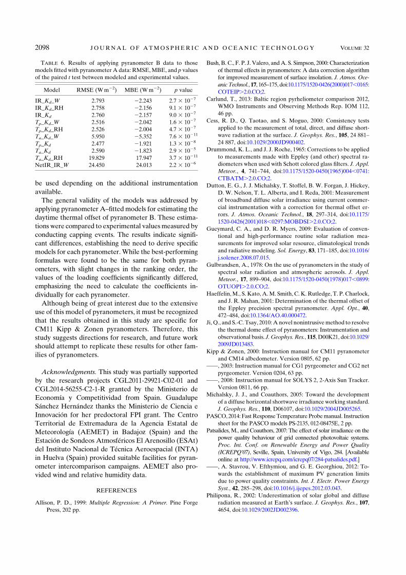
be used depending on the additional instrumentation

available.

The general validity of the models was addressed by

applying pyranometer A–fitted models for estimating the

daytime thermal offset of pyranometer B. These estima-

tions were compared to experimental valuesmeasured by

conducting capping events. The results indicate signifi-

cant differences, establishing the need to derive specific

models for each pyranometer.While the best-performing

formulas were found to be the same for both pyran-

ometers, with slight changes in the ranking order, the

values of the loading coefficients significantly differed,

emphasizing the need to calculate the coefficients in-

dividually for each pyranometer.

Although being of great interest due to the extensive

use of this model of pyranometers, it must be recognized

that the results obtained in this study are specific for

CM11 Kipp & Zonen pyranometers. Therefore, this

study suggests directions for research, and future work

should attempt to replicate these results for other fam-

ilies of pyranometers.

Acknowledgments. This study was partially supported

by the research projects CGL2011-29921-C02-01 and

CGL2014-56255-C2-1-R granted by the Ministerio de

Economía y Competitividad from Spain. Guadalupe

Sánchez Hernández thanks the Ministerio de Ciencia e

Innovación for her predoctoral FPI grant. The Centro

Territorial de Extremadura de la Agencia Estatal de

Meteorología (AEMET) in Badajoz (Spain) and the

Estación de Sondeos Atmosféricos El Arenosillo (ESAt)

del Instituto Nacional de Técnica Aeroespacial (INTA)

in Huelva (Spain) provided suitable facilities for pyran-

ometer intercomparison campaigns. AEMET also pro-

vided wind and relative humidity data.

REFERENCES

Allison, P. D., 1999: Multiple Regression: A Primer. Pine Forge

Press, 202 pp.

Bush, B. C., F. P. J. Valero, andA. S. Simpson, 2000: Characterization

of thermal effects in pyranometers: A data correction algorithm

for improved measurement of surface insolation. J. Atmos. Oce-

anicTechnol., 17, 165–175, doi:10.1175/1520-0426(2000)017,0165:

COTEIP.2.0.CO;2.

Carlund, T., 2013: Baltic region pyrheliometer comparison 2012,

WMO Instruments and Observing Methods Rep. IOM 112,

46 pp.

Cess, R. D., Q. Taotao, and S. Moguo, 2000: Consistency tests

applied to the measurement of total, direct, and diffuse short-

wave radiation at the surface. J. Geophys. Res., 105, 24 881–

24 887, doi:10.1029/2000JD900402.

Drummond, K. L., and J. J. Roche, 1965: Corrections to be applied

to measurements made with Eppley (and other) spectral ra-

diometers when used with Schott colored glass filters. J. Appl.

Meteor., 4, 741–744, doi:10.1175/1520-0450(1965)004,0741:

CTBATM.2.0.CO;2.

Dutton, E. G., J. J. Michalsky, T. Stoffel, B. W. Forgan, J. Hickey,

D. W. Nelson, T. L. Alberta, and I. Reda, 2001: Measurement

of broadband diffuse solar irradiance using current commer-

cial instrumentation with a correction for thermal offset er-

rors. J. Atmos. Oceanic Technol., 18, 297–314, doi:10.1175/

1520-0426(2001)018,0297:MOBDSI.2.0.CO;2.

Gueymard, C. A., and D. R. Myers, 2009: Evaluation of conven-

tional and high-performance routine solar radiation mea-

surements for improved solar resource, climatological trends

and radiative modeling. Sol. Energy, 83, 171–185, doi:10.1016/

j.solener.2008.07.015.

Gulbrandsen, A., 1978: On the use of pyranometers in the study of

spectral solar radiation and atmospheric aerosols. J. Appl.

Meteor., 17, 899–904, doi:10.1175/1520-0450(1978)017,0899:

OTUOPI.2.0.CO;2.

Haeffelin,M., S. Kato,A.M. Smith, C. K.Rutledge, T. P. Charlock,

and J. R. Mahan, 2001: Determination of the thermal offset of

the Eppley precision spectral pyranometer. Appl. Opt., 40,

472–484, doi:10.1364/AO.40.000472.

Ji, Q., and S.-C. Tsay, 2010: A novel nonintrusivemethod to resolve

the thermal dome effect of pyranometers: Instrumentation and

observational basis. J. Geophys. Res., 115, D00K21, doi:10.1029/

2009JD013483.

Kipp & Zonen, 2000: Instruction manual for CM11 pyranometer

and CM14 albedometer. Version 0805, 62 pp.

——, 2003: Instruction manual for CG1 pyrgeometer and CG2 net

pyrgeometer. Version 0204, 63 pp.

——, 2008: Instruction manual for SOLYS 2, 2-Axis Sun Tracker.

Version 0811, 66 pp.

Michalsky, J. J., and Coauthors, 2005: Toward the development

of a diffuse horizontal shortwave irradiance working standard.

J. Geophys. Res., 110, D06107, doi:10.1029/2004JD005265.

PASCO, 2014: FastResponseTemperatureProbemanual. Instruction

sheet for the PASCO models PS-2135, 012-08475E, 2 pp.

Patsalides, M., and Coauthors, 2007: The effect of solar irradiance on the

power quality behaviour of grid connected photovoltaic systems.

Proc. Int. Conf. on Renewable Energy and Power Quality

(ICREPQ’07), Seville, Spain, University of Vigo, 284. [Available

online at http://www.icrepq.com/icrepq07/284-patsalides.pdf.]

——, A. Stavrou, V. Efthymiou, and G. E. Georghiou, 2012: To-

wards the establishment of maximum PV generation limits

due to power quality constraints. Int. J. Electr. Power Energy

Syst., 42, 285–298, doi:10.1016/j.ijepes.2012.03.043.

Philipona, R., 2002: Underestimation of solar global and diffuse

radiation measured at Earth’s surface. J. Geophys. Res., 107,

4654, doi:10.1029/2002JD002396.

TABLE 6. Results of applying pyranometer B data to those

models fitted with pyranometer A data: RMSE,MBE, and p values

of the paired t test between modeled and experimental values.

Model RMSE (Wm22) MBE (Wm22) p value

IR_Kd_W 2.793 22.243 2.7 3 1027

IR_Kd_RH 2.758 22.156 9.1 3 1027

IR_Kd 2.760 22.157 9.0 3 1027

Tp_Kd_W 2.516 22.042 1.6 3 1027

Tp_Kd_RH 2.526 22.004 4.7 3 1027

Ta_Kd_W 5.950 25.352 7.6 3 10211

Tp_Kd 2.477 21.921 1.3 3 1028

Ta_Kd 2.590 21.823 2.9 3 1025

Ta_Kd_RH 19.829 17.947 3.7 3 10211

NetIR_IR_W 24.450 24.013 2.2 3 1026


Reda, I., T. Stoffel, and D. Myers, 2003: A method to calibrate a

solar pyranometer for measuring reference diffuse irradiance.

Sol. Energy, 74, 103–112, doi:10.1016/S0038-092X(03)00124-5.

Sanchez, G., A. Serrano, M. L. Cancillo, and J. A. Garcia, 2015: Pyr-

anometer thermal offset: Measurement and analysis. J. Atmos.

Oceanic Technol., 32, 234–246, doi:10.1175/JTECH-D-14-00082.1.

Smith, A. M., 1999: Prediction and measurement of thermal exchange

within pyranometers. M.S. thesis, Dept. of Mechanical Engi-

neering,Virginia Polytechnic Institute andStateUniversity, 64 pp.

Stine, R. A., 1995: Graphical interpretation of variance inflation

factors. Amer. Stat. Assoc., 49, 53–56.

Vignola, F., C. N. Long, and I. Reda, 2007: Evaluation of methods to

correct for IR loss in Eppley PSP diffusemeasurements.Optical

Modeling and Measurements for Solar Energy Systems, D. R.

Myers, Ed., International Society for Optical Engineering

(SPIE Proceedings, Vol. 6652), 66520A, doi:10.1117/12.734474.

——,——, and——, 2008:Modeling IR radiative loss fromEppley

PSP pyranometer. Optical Modeling and Measurements for

Solar Energy Systems II, B. K. Tsai, Ed., International Society

for Optical Engineering (SPIE Proceedings, Vol. 7046),

70460E, doi:10.1117/12.796457.

——, ——, and ——, 2009: Testing a model of IR radiative losses.

Optical Modeling andMeasurements for Solar Energy Systems

III, B. K. Tsai, Ed., International Society for Optical Engi-

neering (SPIE Proceedings, Vol. 7410), 741003, doi:10.1117/

12.826325.

Wang, K., R. E. Dickinson, Q. Ma, J. A. Augustine, and M. Wild,

2013: Measurement methods affect the observed global dim-

ming and brightening. J. Climate, 26, 4112–4120, doi:10.1175/

JCLI-D-12-00482.1.

WMO, 1996: Guide to Meteorological Instruments and Methods of

Observation. 6th ed. WMO-8, 501 pp.


Copyright of Journal of Atmospheric & Oceanic Technology is the property of AmericanMeteorological Society and its content may not be copied or emailed to multiple sites orposted to a listserv without the copyright holder's express written permission. However, usersmay print, download, or email articles for individual use.

3.3. ARTICULO 2 69


El artıculo “Correcting daytime thermal offset in unventilated pyranometers”,

fue publicado en la revista Journal of Atmospheric and Oceanic Technology en el

ano 2015, teniendo la revista un factor de impacto de 2.159 y estando incluida en el


Ocean”.


artıculo ha sido elevada y diversa, colaborando muy activamente en todas las etapas

desarrolladas para la obtencion del artıculo, como el diseno y realizacion de los

experimentos de medida, la propuesta de modelos de correccion y su implementacion

y calculo, el analisis de resultados y la preparacion del manuscrito.




Por otra parte, D. Antonio Serrano Perez y Dna. Marıa Luisa Cancillo Fernandez,

coautores de este artıculo, afirman mediante este escrito que han colaborado en este

artıculo pero que este forma parte ıntegra de la Tesis Doctoral de Dna. Guadalupe

Sanchez Hernandez y que no va a ser utilizado por ellos como parte de sus respectivas

tesis doctorales.

Dna. Mª Luisa Cancillo Fernandez D. Antonio Serrano Perez


3.4. Artıculo 3


Tıtulo: An intercomparison of the thermal offset for different

pyranometers


Mª Luisa Cancilloa

Antonio Serranoa


Revista: Journal of Geophysical Research - Atmospheres


doi: 10.1002/2016JD024815


Este artıculo amplıa nuestros estudios previos sobre el cero termico aplican-

do la metodologıa de tapado a diversos modelos de piranometro de diferentes

fabricantes. Con este fin se organizo una campana en la que participaron tres

de los principales fabricantes de piranometros, cada uno de las cuales cedio de

forma temporal dos de sus instrumentos mas utilizados. El objetivo ultimo fue

el estudio de las diferencias en magnitud, comportamiento diurno y dependencia

de las condiciones ambientales del cero termico de los piranometros participan-

tes en la campana. Cabe destacar que esta es la campana de intercomparacion

de valores de cero termico con mayor numero de tapados realizada hasta el momento.

Teniendo en cuenta los resultados de los dos artıculos anteriores, se decidio rea-

lizar esta nueva campana durante dos dıas despejados de verano. Estos dıas las

variables que determinan el cero termico, como la temperatura o la propia radiacion

solar, presentan un amplio rango de variacion. Ademas, es en dıas despejados

cuando se esperan los valores mas elevados de cero termico. La distribucion de

los tapados a lo largo de todo el dıa permitio ademas la obtencion de valores de

cero termico bajo condiciones similares de radiacion pero diferentes condiciones de

temperatura, humedad relativa y viento.

Aprovechando que esta nueva campana requerıa de la fabricacion de mas tapas,

se volvio a pensar en el diseno y el proceso de fabricacion de las mismas. Aunque

finalmente se conservo el diseno original, en esta ocasion fabrico un molde con ayuda

de una impresora 3D el cual se relleno con un material aislante. La emisividad

3.4. ARTICULO 3 71

y posible influencia de las tres nuevas tapas se evaluo mediante varios tapados

largos sobre los piranometros y varios tapados sobre el pirgeometro de la nuestra

estacion. Estas pruebas revelaron que la emisividad promedio de las tres tapas es

de 0.4 W/m2. El estudio confirmara que este valor esta muy por debajo de los

valores de cero termico medidos por lo que su efecto puede considerarse despreciable.

Los resultados muestran notables diferencias entre los valores de cero termico de

los piranometros analizados. En las horas centrales del dıa estas diferencias pueden

llegar a alcanzar hasta 8 W/m2. Ademas de las diferencias en los valores del cero

termico se han observado tambien importantes diferencias en su comportamiento

diurno. Si bien el cero termico de todos los piranometro muestran un ciclo diurno,

este mucho mas acusado en unos piranometros que en otros. Estas diferencias entre

piranometros son de gran relevancia tanto en la comparacion de estudios realizados

con diferentes instrumentos como en la continuidad de series largas de radiacion y los

estudios sobre posibles tendencias en los valores de radiacion derivados de su analisis.

Este estudio ratifica las importantes diferencias detectadas en nuestros estudios

anteriores entre el cero termico nocturno y diurno en el piranometro CMP11 y

revela que los nuevos instrumentos analizados en esta campana tambien muestran

esas mismas diferencias. Este resultado advierte sobre la inexactitud que podrıa

cometerse si se corrigen los valores diurnos de cero termico a partir de los valores

nocturnos.

No menos importantes son las diferencias observadas en las dependencias

del cero termico de cada piranometro respecto a las variables meteorologicas

y radiativas analizadas. Este resultado pone de manifiesto la importancia del

diseno y los materiales empleados en la fabricacion del piranometro sobre el cero

termico. Ademas, este resultado muestra la dificultad de establecer un modelo de

correccion comun para todos los piranometros a partir de variables meteorologicas

y/o radiativas. Esto sugiere que los modelos obtenidos en el Artıculo 2 podrıan no

ser validos para todos los instrumentos. Por tanto, se requieren estudios especıficos

para definir la forma mas adecuada de corregir el cero termico en cada tipo de

piranometro.

Un resultado no esperado de este estudio es la no viabilidad de la metodologıa

de tapados para la medida del cero termico en uno de los piranometros inicialmente

considerados. No obstante, la metodologıa ha podido ser aplicada a cinco de los seis

instrumentos con los que se inicio el estudio. Por tanto se puede seguir considerando


una metodologıa de aplicacion general.

A pesar del enorme esfuerzo hecho para medir valores de cero termico en un

amplio rango de valores de temperatura, radiacion, humedad relativa y velocidad

viento este estudio no contempla distintas situaciones nubosas o temperaturas por

debajo de los 15 °C. Aunque en estas situaciones cabrıa esperar valores mas bajos

tanto del cero termico de cada piranometro como de las diferencias entre ellos,

serıa conveniente ampliar el numero de medidas en tales condiciones. Estas nuevas

medidas son imprescindibles para la obtencion de modelos de correccion del cero

termico para cada piranometro.

Dadas las limitaciones de nuestra estacion no pudo hacerse una comparativa

simultanea del cero termico de los cinco piranometros midiendo difusa. Esta

comparativa requiere al menos la instalacion de dos seguidores solares mientras que

nuestra estacion solo cuenta con uno. Una comparativa de este tipo podrıa ayudar

a esclarecer la existencia o no de diferencias en los valores de cero termico entre las

medidas de irradiancia global y difusa.


An intercomparison of the thermal offsetfor different pyranometersG. Sanchez1, M. L. Cancillo1, and A. Serrano1

1Department of Physics, University of Extremadura, Badajoz, Spain

Abstract An unprecedented intensive intercomparison campaign focused on the experimental measurementof the thermal offset of pyranometers has been conducted at Badajoz (Spain) with the participation of three mainmanufacturers. The purpose of this study is to compare the thermal offset of six commercially availablepyranometers, being some of them widely used and others recently commercialized. In this campaign, thecappingmethodology has been used to experimentally measure the daytime thermal offset of the pyranometers.Thus, a short but intense campaign has been conducted in two selected summer days under clear-sky conditions,covering a large range of solar zenith angle, irradiance, and temperature. Along the campaign, a total of 305capping events have been performed, 61 for each pyranometer. The daytime thermal offset obtained for differentpyranometers ranges between 0 and�16.8W/m2 depending on the environmental conditions, being sometimesnotably higher than values estimated indoors by manufacturers. The thermal offset absolute value of allinstruments shows a diurnal cycle, increasing from sunrise to central hours of the day and decreasing frommidafternoon to sunset. The analysis demonstrates that thermal offset is notably higher andmore variable duringdaytime than during nighttime, requiring specific daytime measurements. Main results emphasize the key roleplayed by wind speed in modulating the thermal offset.

1. Introduction

Very accurate measurements of global irradiance on the Earth’s surface are currently demanded in order todetect small variations in the incoming solar radiation and therefore changes in climate. Thus, variations in theamount of solar energy reaching the Earth’s surface could have profound environmental, social, and economicimplications [Wild, 2009]. A first evidence of secular variations in solar radiation on the Earth’s surface wasreported in late 1980s and early 1990s [Ohmura and Lang, 1989; Russak, 1990; Dutton et al., 1990]. From thenon, numerous studies have analyzed the trend of mean global irradiance on the Earth’s surface [Wild, 2009].Wild et al. [2005] quantified these variations to be between �5.1W/m2 and �1.6W/m2 per decade during thedimming period (1960–1990) and between +2.2W/m2 and +5.1W/m2 per decade during the brightening period(after 1990). This trend has been confirmed by later studies [Sanchez-Lorenzo et al., 2015; Wild, 2016]. However,the responsible for this change is not clear, and thus, the contribution of clouds and aerosols to the decadal var-iations of global irradiance is still a controversial topic [Wild, 2009; Augustine and Dutton, 2013;Mateos et al., 2014].

This growing interest for accurate irradiance measurements on the Earth’s surface has favored the deploymentof a great number of ground-based radiation networks (Global Energy Budget Archive, Baseline SurfaceRadiation Network, Surface Radiation, Atmospheric Radiation Measurement Program, etc.). Pyranometersinstalled in these radiometric stations must satisfy quality requirements established by World MeteorologicalOrganization (WMO) [2008] to provide high quality; however, each manufacturer chooses specific designsand materials to comply with these requirements. The final design and materials have relevant influence onthe pyranometer performance and therefore on the uncertainty of its measurements.

An important source of uncertainty is their thermal offset error [Philipona, 2002]. Thermal offset is an spurioussignal caused by the difference in temperature between the dome and the detector of a pyranometer. Thethermal offset has been quantified to be between �30W/m2 and �5W/m2 depending on the instrumentdesign and environmental conditions [Reda et al., 2003; Ji, 2007]. Several studies [Bush et al., 2000; Sanchezet al., 2015] have reported notable differences in thermal offset between overcast or cloud-free conditions.The effect of thermal offset in irradiance values could range from 1% for irradiance during cloudy days to15% for diffuse irradiance during cloud-free days [Sanchez et al., 2015]. The decrease in thermal offset undercloudy conditions is mainly due to the enhancement of downward IR by clouds, which reduces the dome-detector temperature difference. Additionally, a direct relationship between thermal offset and ambient

SANCHEZ ET AL. THERMAL OFFSET INTERCOMPARISON 7901

PUBLICATIONSJournal of Geophysical Research: Atmospheres

RESEARCH ARTICLE10.1002/2016JD024815

Key Points:• First intensive intercomparisoncampaign of pyranometer thermaloffset with the main manufacturers

• Daytime thermal offset differsbetween instruments, ranging mostlybetween 0 and -10 W/m²

• Daytime thermal offset in clear skiesshows a diurnal cycle being windspeed a key factor

Correspondence to:G. Sanchez,[email protected]

Citation:Sanchez, G., M. L. Cancillo, and A.Serrano (2016), An intercomparison ofthe thermal offset for different pyran-ometers, J. Geophys. Res. Atmos., 121,7901–7912, doi:10.1002/2016JD024815.

Received 18 JAN 2016Accepted 12 JUN 2016Accepted article online 15 JUN 2016Published online 4 JUL 2016

©2016. American Geophysical Union.All Rights Reserved.

temperature has been suggested by several authors [Haeffelin et al., 2001; Dutton et al., 2001; Ji and Tsay,2010; Sanchez et al., 2015; Serrano et al., 2015]. The uncertainty caused by the thermal offset can be very largecompared with trends observed in mean global irradiance at the Earth’s surface and therefore must beaccounted for in radiative forcing studies.

The thermal offset effect is a well-known issue for pyranometers. Indeed, it was detected in the early opera-tions of pyranometers [Drummond and Roche, 1965], but its effect in the uncertainty of shortwave irradiancemeasurements has been ignored until recently. Additionally, most previous studies treated the thermal offsetas an additional correction in a preprocessing stage [Philipona, 2002; Michalsky et al., 2003, 2005; Carlund,2013] or focused on a particular pyranometer model under specific conditions [Bush et al., 2000; Haeffelinet al., 2001; Ji and Tsay, 2010; Ji et al., 2011]. Only a few studies have compared various pyranometers[Philipona, 2002;Michalsky et al., 2003, 2005; Ji, 2007; Carlund, 2013], and they have the drawback of compar-ing against a zero-thermal offset reference, ignoring other sources of differences among instruments.

The limitations in previous studies and the introduction of new and improved pyranometer models in radio-metric stations worldwide motivates a updated approach to the study of thermal offset. Additionally, a com-prehensive study of the thermal offset requires comparing different pyranometer models under the sameenvironmental and radiative conditions. Such intercomparison is needed to put into agreement the conclu-sions reported by different authors using different types of pyranometers.

Thus, this paper presents an intercomparison of the thermal offset between different unventilated pyran-ometers. Toward that aim, a specific intensive campaign was organized and the main manufacturers wereinvited to send their instruments. Six pyranometers participated in the campaign, being four of them widelyused instruments and the other two newmodels recently commercialized. During this campaign, the thermaloffset of the six pyranometers were measured simultaneously by means of the capping methodology, andsubsequently compared. This study aims at analyzing differences in magnitude, diurnal behavior, and depen-dence on environmental conditions. This is, to our knowledge, the first intensive thermal offset intercompar-ison for pyranometers using the capping methodology. This analysis could have profound implications in thehomogenization of long-term radiation series for climate and radiative forcing analysis.

2. Instrumentation

The measurements were performed in June 2015 at the radiometric station installed in Badajoz, southwes-tern Spain (38.98°N, 7.018°W; 199m above sea level), on the roof of the Department of Physics’ building atthe campus of the University of Extremadura, guaranteeing an open horizon. This radiometric station is man-aged by the “Atmosphere, Climate and Radiation in Extremadura” research group of the University ofExtremadura. Badajoz is located in south-western Spain, being characterized by amild Mediterranean climatewith very dry and hot summer and solar irradiance values among the highest recorded in Europe in summer.

In order to perform a comprehensive study, the main manufacture of pyranometers were invited to participatein the campaign and six instruments, provided by Eppley (SPP and GPP), Hukseflux (SR20 and SR25), and Kipp &Zonen (CMP11 and CMP22), were compared. Each manufacturer contributed with two different pyranometers:a widely used model and a new or improved version. All these pyranometers comply with InternationalOrganization for Standardization (ISO) 9060 criteria for an ISO secondary standard pyranometer, being classifiedas “high quality” according to theWorld Meteorological Organization (WMO) nomenclature [WMO, 2008]. Thesepyranometers are calibrated according to procedures detailed in International Organization for Standardization(ISO) 9847 [1992]. Table 1 summarizes their main characteristics as reported in the corresponding pyranometermanuals and manufacturer websites [Kipp and Zonen, 2013; Hukseflux, 2014, 2015; https://eppleylab.com].

The fundamental basis of operation for the participating pyranometers is the thermoelectric principle. Theirsensing elements are made up of a large number of thermocouples junction pairs connected in series. Whilethe reference junction keeps at a fixed temperature, the active junction is exposed to the solar radiation.Bonded on the active junctions to the thermocouples there is a black-painted ceramic disk that help toabsorb the incident solar radiation. When the incoming radiation passes through the two glass domes, it isabsorbed by the black ceramic disk making the temperature of the active junctions increases. The differentialtemperature between the active and the reference junctions produces an electromotive force directly pro-portional to the differential temperature created, and subsequently a voltage signal.

Journal of Geophysical Research: Atmospheres 10.1002/2016JD024815


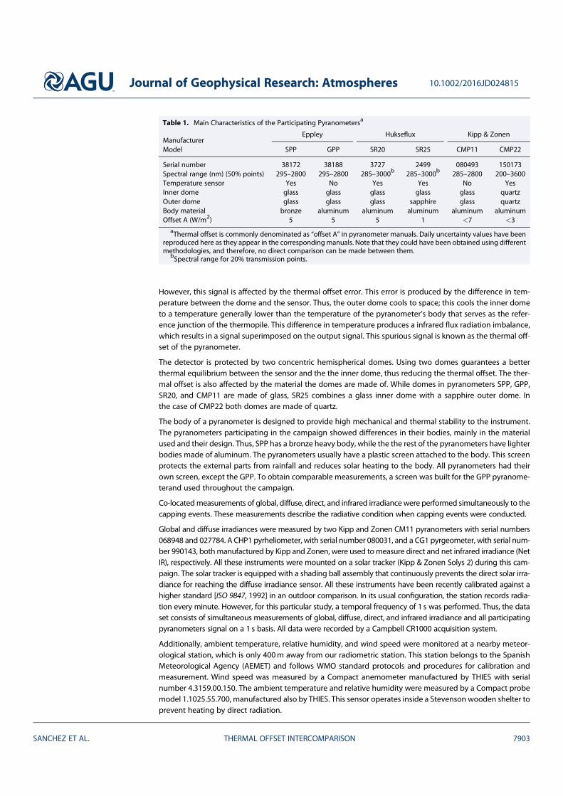
However, this signal is affected by the thermal offset error. This error is produced by the difference in tem-perature between the dome and the sensor. Thus, the outer dome cools to space; this cools the inner dometo a temperature generally lower than the temperature of the pyranometer’s body that serves as the refer-ence junction of the thermopile. This difference in temperature produces a infrared flux radiation imbalance,which results in a signal superimposed on the output signal. This spurious signal is known as the thermal off-set of the pyranometer.

The detector is protected by two concentric hemispherical domes. Using two domes guarantees a betterthermal equilibrium between the sensor and the the inner dome, thus reducing the thermal offset. The ther-mal offset is also affected by the material the domes are made of. While domes in pyranometers SPP, GPP,SR20, and CMP11 are made of glass, SR25 combines a glass inner dome with a sapphire outer dome. Inthe case of CMP22 both domes are made of quartz.

The body of a pyranometer is designed to provide high mechanical and thermal stability to the instrument.The pyranometers participating in the campaign showed differences in their bodies, mainly in the materialused and their design. Thus, SPP has a bronze heavy body, while the the rest of the pyranometers have lighterbodies made of aluminum. The pyranometers usually have a plastic screen attached to the body. This screenprotects the external parts from rainfall and reduces solar heating to the body. All pyranometers had theirown screen, except the GPP. To obtain comparable measurements, a screen was built for the GPP pyranome-terand used throughout the campaign.

Co-locatedmeasurements of global, diffuse, direct, and infrared irradiancewere performed simultaneously to thecapping events. These measurements describe the radiative condition when capping events were conducted.

Global and diffuse irradiances were measured by two Kipp and Zonen CM11 pyranometers with serial numbers068948 and 027784. A CHP1 pyrheliometer, with serial number 080031, and a CG1 pyrgeometer, with serial num-ber 990143, bothmanufactured by Kipp and Zonen, were used tomeasure direct and net infrared irradiance (NetIR), respectively. All these instruments were mounted on a solar tracker (Kipp & Zonen Solys 2) during this cam-paign. The solar tracker is equipped with a shading ball assembly that continuously prevents the direct solar irra-diance for reaching the diffuse irradiance sensor. All these instruments have been recently calibrated against ahigher standard [ISO 9847, 1992] in an outdoor comparison. In its usual configuration, the station records radia-tion every minute. However, for this particular study, a temporal frequency of 1 s was performed. Thus, the dataset consists of simultaneous measurements of global, diffuse, direct, and infrared irradiance and all participatingpyranometers signal on a 1 s basis. All data were recorded by a Campbell CR1000 acquisition system.

Additionally, ambient temperature, relative humidity, and wind speed were monitored at a nearby meteor-ological station, which is only 400m away from our radiometric station. This station belongs to the SpanishMeteorological Agency (AEMET) and follows WMO standard protocols and procedures for calibration andmeasurement. Wind speed was measured by a Compact anemometer manufactured by THIES with serialnumber 4.3159.00.150. The ambient temperature and relative humidity were measured by a Compact probemodel 1.1025.55.700, manufactured also by THIES. This sensor operates inside a Stevenson wooden shelter toprevent heating by direct radiation.

Table 1. Main Characteristics of the Participating Pyranometersa

ManufacturerEppley Hukseflux Kipp & Zonen

Model SPP GPP SR20 SR25 CMP11 CMP22

Serial number 38172 38188 3727 2499 080493 150173Spectral range (nm) (50% points) 295–2800 295–2800 285–3000b 285–3000b 285–2800 200–3600Temperature sensor Yes No Yes Yes No YesInner dome glass glass glass glass glass quartzOuter dome glass glass glass sapphire glass quartzBody material bronze aluminum aluminum aluminum aluminum aluminumOffset A (W/m2) 5 5 5 1 <7 <3

aThermal offset is commonly denominated as “offset A” in pyranometer manuals. Daily uncertainty values have beenreproduced here as they appear in the corresponding manuals. Note that they could have been obtained using differentmethodologies, and therefore, no direct comparison can be made between them.

bSpectral range for 20% transmission points.



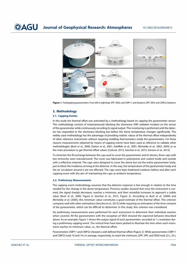
3. Methodology3.1. Capping Events

In this study the thermal offset was estimated by a methodology based on capping the pyranometer sensor.This methodology consists of instantaneously blocking the shortwave (SW) radiation incident on the sensorof the pyranometer while continuously recording its signal output. This monitoring is performed until the detec-tor has responded to the shortwave blocking but before the dome temperature changes significantly. Thiswidely used methodology has the advantage of providing realistic values of the thermal offset independentlyof other reference instruments without requiring installing thermometers inside the pyranometers. For thesereasons measurements obtained by means of capping events have been used as reference to validate othermethodologies [Bush et al., 2000; Dutton et al., 2001; Haeffelin et al., 2001; Michalsky et al., 2003, 2005] or asthe main procedure to get thermal offset values [Carlund, 2013; Sanchez et al., 2015; Serrano et al., 2015].

To minimize the IR exchange between the cap used to cover the pyranometer and its domes, three caps withlow emissivity were manufactured. The cover was fabricated in polystyrene and coated inside and outsidewith a reflective material. The caps were designed to cover the dome but not the entire pyranometer body,just to block the irradiance arriving at the detector. In this way, the temperature of the pyranometer body andthe air circulation around it are not affected. The caps were kept shadowed outdoors before and after eachcapping event with the aim of maintaining the caps at ambient temperature.

3.2. Preliminary Measurements

The capping event methodology assumes that the detector response is fast enough in relation to the timeneeded for the change in the dome temperature. Previous studies showed that once the instrument is cov-ered, the signal sharply decreases, reaches a minimum, and then smoothly increases to approach a stablevalue [Bush et al., 2000, Figure 6; Sanchez et al., 2015, Figure 2]. According to Bush et al. [2000] andMichalsky et al. [2005], this minimum value constitutes a good estimate of the thermal offset. This criterioncompares well with other estimations [Sanchez et al., 2015] while requiring no estimation of the time constantof the pyranometer, which can be difficult to determine. In this study, this criterion was considered.

Six preliminary measurements were performed for each instrument to determine their individual reactionwhen covered. All the pyranometers with the exception of SR25 showed the expected behavior describedabove. As an example, Figure 1 shows the output signal of each pyranometer, recorded at 1 s resolution dur-ing a preliminary capping event. The vertical lines have been plotted to illustrate the time when each instru-ment reaches its minimum value, i.e., the thermal offset.

Pyranometers CMP11 and CMP22 showed a well-defined thermal offset (Figure 2). While pyranometers CMP11and CMP22 took 10 and 14 s in average, respectively, to reach the minimum, GPP, SPP, and SR20 took 22 s, 33 s,

Figure 1. Participating pyranometers. From left to right:(top) SPP, SR20, and CMP11 and (bottom) GPP, SR25 and CMP22 (bottom).



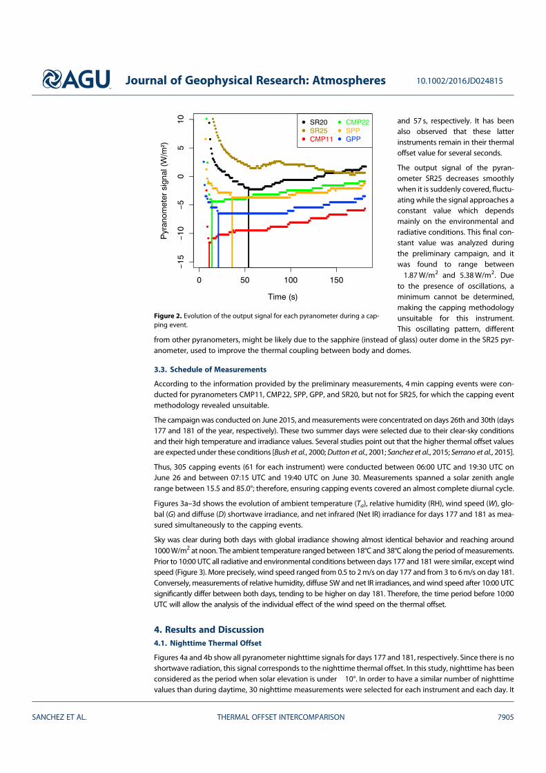
and 57 s, respectively. It has beenalso observed that these latterinstruments remain in their thermaloffset value for several seconds.

The output signal of the pyran-ometer SR25 decreases smoothlywhen it is suddenly covered, fluctu-ating while the signal approaches aconstant value which dependsmainly on the environmental andradiative conditions. This final con-stant value was analyzed duringthe preliminary campaign, and itwas found to range between�1.87W/m2 and 5.38W/m2. Dueto the presence of oscillations, aminimum cannot be determined,making the capping methodologyunsuitable for this instrument.This oscillating pattern, different

from other pyranometers, might be likely due to the sapphire (instead of glass) outer dome in the SR25 pyr-anometer, used to improve the thermal coupling between body and domes.

3.3. Schedule of Measurements

According to the information provided by the preliminary measurements, 4min capping events were con-ducted for pyranometers CMP11, CMP22, SPP, GPP, and SR20, but not for SR25, for which the capping eventmethodology revealed unsuitable.

The campaign was conducted on June 2015, andmeasurements were concentrated on days 26th and 30th (days177 and 181 of the year, respectively). These two summer days were selected due to their clear-sky conditionsand their high temperature and irradiance values. Several studies point out that the higher thermal offset valuesare expected under these conditions [Bush et al., 2000;Dutton et al., 2001; Sanchez et al., 2015; Serrano et al., 2015].

Thus, 305 capping events (61 for each instrument) were conducted between 06:00 UTC and 19:30 UTC onJune 26 and between 07:15 UTC and 19:40 UTC on June 30. Measurements spanned a solar zenith anglerange between 15.5 and 85.0°; therefore, ensuring capping events covered an almost complete diurnal cycle.

Figures 3a–3d shows the evolution of ambient temperature (Ta), relative humidity (RH), wind speed (W), glo-bal (G) and diffuse (D) shortwave irradiance, and net infrared (Net IR) irradiance for days 177 and 181 as mea-sured simultaneously to the capping events.

Sky was clear during both days with global irradiance showing almost identical behavior and reaching around1000W/m2 at noon. The ambient temperature ranged between 18°C and 38°C along the period ofmeasurements.Prior to 10:00 UTC all radiative and environmental conditions between days 177 and 181were similar, except windspeed (Figure 3). More precisely, wind speed ranged from 0.5 to 2m/s on day 177 and from 3 to 6m/s on day 181.Conversely, measurements of relative humidity, diffuse SW and net IR irradiances, and wind speed after 10:00 UTCsignificantly differ between both days, tending to be higher on day 181. Therefore, the time period before 10:00UTC will allow the analysis of the individual effect of the wind speed on the thermal offset.

4. Results and Discussion4.1. Nighttime Thermal Offset

Figures 4a and 4b show all pyranometer nighttime signals for days 177 and 181, respectively. Since there is noshortwave radiation, this signal corresponds to the nighttime thermal offset. In this study, nighttime has beenconsidered as the period when solar elevation is under �10°. In order to have a similar number of nighttimevalues than during daytime, 30 nighttime measurements were selected for each instrument and each day. It

Figure 2. Evolution of the output signal for each pyranometer during a cap-ping event.



can be seen that this nighttime thermal offset is very stable as compared with the daytime estimationsobtained by capping events (Figures 4c and 4d). The standard deviation of the nighttime thermal offsetranges from 0.30 to 0.61W/m2. Nighttime thermal offset absolute values are also notably lower than thosemeasured during daytime. According to the nighttime mean values, the pyranometers clustered into threegroups: (1) SR25, with a mean value around 0.4W/m2; (2) SR20 and CMP22, with a mean value around�1.5W/m2; and (3) CMP11, SPP, and GPP, with a mean value of �3.5W/m2, more than twice the value ofthe first group. These notable differences between nighttime and daytime thermal offset behavior indicatethe important role played by the radiative and environmental conditions.

4.2. Daytime Thermal Offset

Figures 4c and 4d show the daytime thermal offset obtained by capping events on days 177 and 181. It showsa marked diurnal cycle with a variation 2 or 3 times higher than those observed for nighttime values.

Figure 3. Daily evolution of ambient temperature, global, diffuse, and net IR irradiance, wind speed, and relative humidityfor the two days of cappings (days 177 and 181), measured simultaneously to the capping events.



The vertical lines have been drawn in Figures 4c and 4d to separate time periods when thermal offset showsdifferent overall behavior. Before around 08:00 UTC, absolute values of thermal offset tend to increase for allinstruments. This increase is particularly notable for CMP11, with positive trend until 10:00 UTC. All environ-mental and radiative magnitudes showed high variations during this time period of increasing absolute ther-mal offset, except the wind speed which remained fairly constant. Increasing ambient temperatures, globaland diffuse irradiances, simultaneously to decreasing net IR irradiance and relative humidity, favor theincrease in the absolute value of the thermal offset [Sanchez et al., 2015; Serrano et al., 2015]. The oppositesituation occurs around sunset, explaining the decrease in the absolute thermal offset observed from around17:00 UTC onward.

During the central hours of the day, no overall trend is found, although thermal offset significantly fluctuatesaround the mean value. This high variability agrees with results reported by Haeffelin et al. [2001] for a PSPpyranometer. They explained this variability by the turbulent convective heat exchange between the ambi-ent air and the pyranometer, affecting differently the dome and the body. Some main statistics (mean andstandard deviation) of the thermal offset measured between 10:00 UTC and 17:00 UTC are shown inTable 2 for each pyranometer. Large differences in the thermal offset between pyranometers and time ofthe day are observed. CMP11 shows the highest mean absolute value in both days, followed by GPP andCMP22. On day 177, CMP11 shows notably higher absolute values than the other pyranometers, reachinga maximum absolute value of 16.8W/m2 while the others remain under 10.0W/m2. On the other hand, pyr-anometers SR20 and SPP show the minimummean absolute thermal offset but also the highest variability forboth days. These two pyranometers show very similar statistics for both days.

Figure 4. Thermal offset measured (top row) nighttime and (bottom row) daytime during days 177 and 188.



It is interesting to note the notablereduction on the absolute value ofthe thermal offset of pyranometerCMP22 with respect to CMP11,both manufactured by Kipp &Zonen. Thus, mean absolute valueat central hours of the day forCMP22 is 8W/m2 lower than forCMP11 on day 177 and 4W/m2 onday 181 (Table 2). These high dif-ferences could be due to the differ-

ent design and material of their domes; while CMP11 has two 2mm thick domes made of glass, CMP 22 hastwo 4mm thick domes made of quartz.

Regarding pyranometers SPP and GPP manufactured by Eppley, differences around 3.5W/m2 have also beenobserved. Since both pyranometers have the same type of thermopile and domes, the differences must beassociated with their different body’s material. Thus, while GPP’s body is made of aluminum, SPP’s body ismade of bronze being therefore notably heavier than GPP and showing a lower thermal conductivity.

It is interesting to note that the absolute value of thermal offset obtained experimentally in this study can besignificantly higher than those offset A values provided by manufacturers (see Table 1). The main reason forthese differences is that manufacturers generally measure the offset A under specific conditions, which couldbe notably different from those affecting the instruments outdoors once installed. When a pyranometer isinstalled outdoors at a station additional factors affect its response such as the relative humidity and windspeed. It is also important to note that these factors show different behavior between day and night. A thor-ough analysis about these factors will be developed in section 4.3.

4.3. Dependence on Environmental Magnitudes

In addition to the diurnal cycle, thermal offset varied between days, being remarkably higher on day 177 thanon day 181. Also, day 171 showed a larger variability than day 181.

It is not easy to identify the main factors explaining the differences in thermal offset between days 177 and181 since many radiative and environmental variables generally differ between the two days. However, thereis a rather interesting time period before 10:00 UTC, when all radiative and environmental conditions exceptthe wind speed behave similarly on days 177 and 181 (Figure 3). Thus, for this time period, differences in ther-mal offset between both days can be attributed to the effect of wind speed.

In order to analyze the effect of this and other environmental magnitudes, a thorough analysis has been per-formed. Figure 5 show the daytime and nighttime thermal offset versus wind speed, Net IR irradiance, ambi-ent temperature, and relative humidity for each pyranometer.

Significant differences in behavior are observed between day and nighttime thermal offset and betweentheir relationships with the environmental conditions. A main limitation is the short range of variation ofenvironmental conditions during night, showing no clear trend and therefore preventing developing any lin-ear regression. During nighttime the thermal offset tends to smoothly oscillate around the mean value givenin section 4.1. An additional difference bewteen day and nighttime thermal offset is the lack of solar radiationduring the night, which is acknowledged as a main contribution to the differential heating of the dome andthe sensor and, subsequently, to the thermal offset [Sanchez et al., 2015]. This different behavior betweendaytime and nighttime is in agreement with results reported by several other authors who prevent correctingdaytime thermal offset using empirical models developed with nighttime data [Cess et al., 2000; Haeffelinet al., 2001; Philipona, 2002; Ji and Tsay, 2010; Serrano et al., 2015].

A general negative trend in daytime thermal offset with respect to the ambient temperature can be observedfor all pyranometers. Thus, the absolute value of the thermal offset increases as ambient temperatureincreases. On the contrary, a positive trend is observed in daytime thermal offset with respect to relativehumidity, Net IR, and wind speed for all pyranometer. These findings agree with results reported by otherauthors such as Dutton et al. [2001] and Serrano et al. [2015] and confirm that thermal offset increases under

Table 2. Mean Values and Standard Deviation (SD) of the Thermal Offsetfor Each Instrument on Days 177 and 181 for the Time Period Between10:00 and 17:00 UTC

Day 177 (10:00–17:00 UTC) Day 181 (10:00–17:00 UTC)

Instrument Mean (W/m2) SD (W/m2) Mean (W/m2) SD (W/m2)

SR20 �6.9 2.0 �2.4 1.4CMP11 �15.2 1.0 �9.4 1.1CMP22 �7.2 1.3 �5.4 0.9SPP �6.8 2.1 �2.3 1.5GPP �9.6 2.0 �6.2 0.8



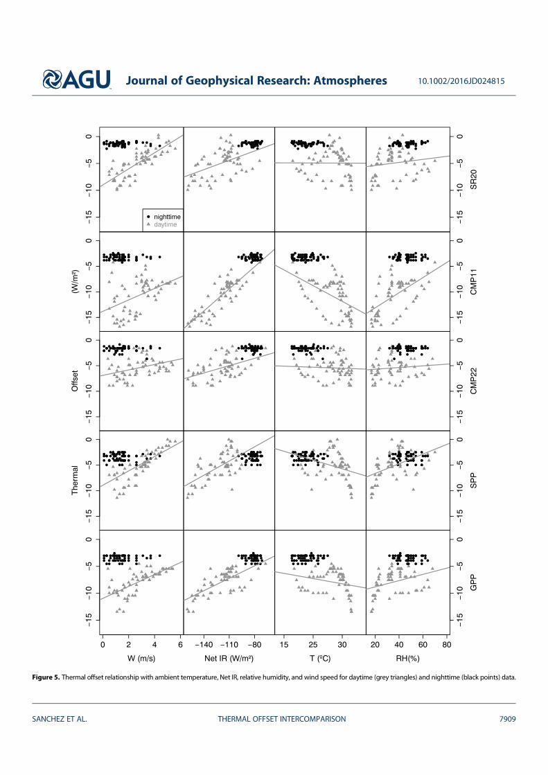
Figure 5. Thermal offset relationship with ambient temperature, Net IR, relative humidity, and wind speed for daytime (grey triangles) and nighttime (black points) data.



cloud-free conditions, low relative humidity, low wind speed, and high temperature. The least squares regres-sion analysis has been conducted to assess the significance of the relationships. The coefficients of determi-nation for these fittings are summarized in Table 3.

The relationships between the thermal offset and ambient temperature and relative humidity are not statis-tically significant, showing values of R2 below 0.4 for all pyranometers. Three pyranometers show R2 valueshigher than 0.4 for fittings with respect to the Net IR being the CMP11 pyranometer, the instrument withthe most significant value (0.739). The relationship with respect to the wind speed is particularly clear for pyr-anometers SR20, SPP, and GPP, with coefficients of determination of 0.64, 0.47, and 0.47, respectively.Therefore, the wind speed appears as a main factor for reducing the absolute value of the thermal offset.This result agrees with Dutton et al. [2001], Michalsky et al. [2005], Ji [2007], and Serrano et al. [2015].

5. Conclusions

In order to thoroughly analyze the thermal offset of different pyranometers, an intensive campaign of mea-surements was conducted at Badajoz (Spain) in June 2015. Pyranometers SR20 and SR25, manufactured byHukseflux; SPP and GPP, manufactured by Eppley; and CMP11 and CMP22, manufactured by Kipp &Zonen, participated in the intercomparison campaign. These pyranometers are a significant representationof widely used and new pyranometer models of the main manufacturers. In this campaign, the thermal offsetwas estimated following the nonintrusive capping methodology.

Preliminary measurements revealed the unsuitability of the capping methodology to be applied to pyran-ometer model SR25 since a clear minimum could not be identified during the capping events. When thisinstrument is covered, its output signal decreases and then tends to oscillate between �1.87W/m2 and5.38W/m2, depending on the environmental and radiative conditions. Therefore, alternative methodologies,such as its comparison with an instrument with negligible thermal offsets or invasive methods as attachingthe installation of temperature sensors on its detector and dome to measure their temperature differencecould be considered.

Regarding nighttime thermal offset, pyranometers clustered into two groups: (1) SR20 and CMP22, with amean value around �1.5W/m2, and (2) CMP11, SPP and GPP, with a mean value of �3.5W/m2. These valuesare notably lower and more stable than those observed during daytime. These values agree with thosereported by Cess et al. [2000], Philipona [2002], Ji and Tsay [2010], and Sanchez et al. [2015] for several unven-tilated pyranometer models and locations. This finding advises, as suggested by Serrano et al. [2015] forCMP11 pyranometers, against the common procedure of estimating diurnal thermal offset from nighttimedata for unventilated pyranometers. However, it should be note that different results could be found for ven-tilated pyranometer, as suggested by Michalsky et al. [2003, 2005].

During the campaign, more than 300 capping events were conducted on clear-sky days 177 and 181 coveringa wide range of solar zenith angle. As a result, a large number of daytime thermal offset values were esti-mated for pyranometers SR20, SPP, GPP, CMP11, and CMP22 under different environmental and radiativeconditions. These measurements revealed a diurnal overall pattern in the absolute values of thermal offset:increasing until around 08:00 UTC or 10:00 UTC, oscillating around a mean value during central hours ofthe day, and decreasing after 17:00 UTC. This diurnal behavior is more notable for CMP11, and its amplitudelikely depends on the environmental and radiative conditions. This diurnal pattern has not been reportedpreviously. Therefore, correcting the thermal offset error requires complex expressions, which account forthis diurnal variation, and not only the addition of a constant factor.

Table 3. Coefficient of Determination, R2, for the Relationships Between the Daytime Thermal Offset and theEnvironmental Magnitudes

Instrument Wind Speed Net IR Ambient Temperature Relative Humidity

SR20 0.640 0.208 0.022 0.024CMP11 0.202 0.739 0.260 0.366CMP22 0.136 0.240 0.003 0.013SPP 0.470 0.423 0.120 0.220GPP 0.470 0.490 0.060 0.125



On average, during the central hours of the day, SPP and SR20 show the lowest absolute value of thermal off-set followed by CMP22 and GPP, while CMP11 tends to show higher absolute values. On the contrary, CMP11,CMP22, and GPP show lower standard deviation than SR20 and SPP. The mean thermal offset during centralhours of the day ranges between �2.3W/m2 and �15.2W/m2. Meanwhile, its standard deviation rangesbetween 0.8W/m2 and 2.1W/m2. It is important to note that a high variability makes it difficult to correctthe thermal offset, while a high but constant value is easier to correct.

During these two days the measured thermal offset resulted in relative errors between 1% and 3%. Thesevalues could result in systematic uncertainties of the order of the 2% established byWMO for daily achievableuncertainty for high-quality pyranometers [WMO, 2008]. This fact emphasizes the need for correcting thissource of error.

The relationship between the themal offset of each pyranometer versus several environmental magnitudes hasbeen analyzed for both daytime and nighttime data. Notable differences in the thermal offset trends betweendaytime and nighttime were detected. This important result agree with results reported by Cess et al. [2000],Philipona [2002], Ji and Tsay [2010] and, more recently, Sanchez et al. [2015] and Serrano et al. [2015]. This findingprevent correcting daytime thermal offset using empirical models developed with nighttime data.

Positive general trends with respect to Net IR, wind speed, and relative humidity and negative trend withrespect to ambient temperature have been found for daytime thermal offset. However, not all these relation-ships are actually significant, and only SR20 thermal offset versus wind speed and CMP11 versus Net IR showR2 values higher than 0.6. Additionally, SPP and GPP thermal offset versus both Net IR and wind speed have R2

values around 0.45. Thus, daytime values of Net IR and wind speed could be considered in order to develop amodel for correcting these instruments as suggested Serrano et al. [2015]. Additionally, this results revealedthat wind speed is a main factor for reducing the magnitude of the thermal offset. This result agrees withprevious studies which suggested that wind speed homogenizes the temperature balance and thereforecontributes to reduce the absolute value of the thermal offset [Bush et al., 2000; Haeffelin et al., 2001;Michalsky et al., 2005; Ji, 2007].

This unprecedented campaign contributes to a better knowledge of the thermal offset of pyranometers bycomparing different instruments under actual measuring conditions outdoors. It provides useful informationthat completes the indoor measurements performed by the manufacturers. Therefore, it favors the precisemeasurement of the Earth’s radiation balance and aerosol radiative forcing, for instance. This study also sug-gests interesting directions for future research concerning the behavior of the thermal offset when the pyr-anometer is ventilated.

ReferencesAugustine, J. A., and E. G. Dutton (2013), Variability of the surface radiation budget over the United States from 1996 through 2011 from high-

quality measurements, J. Geophys. Res. Atmos., 118, 43–53, doi:10.1029/2012JD018551.Bush, B. C., F. P. J. Valero, and A. S. Simpson (2000), Characterization of thermal effects in pyranometers: A data correction algorithm for

improved measurement of surface insolation, J. Atmos. Oceanic Technol., 17, 165–175.Carlund T. (2013), Baltic Region Pyrheliometer Comparison 2012, World Meteorological Organization, Rep. 112, pp. 10–35, Geneva,

Switzerland.Cess, R. D., T. Qian, and M. Sun (2000), Consistency test applied to the measurement of total, direct, and diffuse shortwave radiation at the

surface, J. Geophys. Res., 105, 24,881–24,887.Drummond, K. L., and J. J. Roche (1965), Corrections to be applied to measurements made with Eppley (and other) spectral radiometers

when used with Schott colored glass filters, J. Appl. Meteorol., 4, 741–744.Dutton, E. G., R. S. Stone, D. W. Nelson, and B. G. Mendonca (1990), Recent interannual variations in solar radiation cloudiness, and surface

temperature at the South Pole, J. Clim., 4, 848–858.Dutton, E. G., J. J. Michalsky, T. Stoffel, B. W. Forgan, J. Hickey, D. W. Nelson, T. L. Alberta, and I. Reda (2001), Measurement of broadband

diffuse solar irradiance using current commercial instrumentation with a correction for thermal offset errors, J. Atmos. Oceanic Technol., 18,297–314.

Haeffelin, M., S. Kato, A. M. Smith, C. K. Rutledge, T. P. Charlock, and J. R. Mahan (2001), Determination of the thermal offset of the Eppleyprecision spectral pyranometer, Appl. Opt., 4, 472–484.

Hukseflux (2014), User manual SR20 secondary standard pyranometer, Manual v1407.Hukseflux (2015), User manual SR25 secondary standard pyranometer with sapphire outer dome, Manual v1508.International Organization for Standardization (ISO) 9847 (1992), Solar energy—Calibration of field pyranometers by comparison to a

reference pyranometer.Ji, Q. (2007), A method to correct the thermal dome effect of pyranometers in selected historical solar irradiance measurements, J. Atmos.

Oceanic Technol., 24, 529–536.Ji, Q., and S.-C. Tsay (2010), A novel nonintrusive method to resolve the thermal-dome-effect of pyranometers: Instrumentation and

observational basis, J. Geophys. Res., 115, D00K21, doi:10.1029/2009JD013483.



AcknowledgmentsThis study was partially supported bythe research projects CGL2011-29921-C02-01 and CGL2014-56255-C2-1-Rgranted by the Ministerio de Economíay Competitividad from Spain and byAyuda a Grupos GR15137 granted byJunta de Extremadura and Fondo SocialEuropeo (FEDER). Authors thank Eppley,Hukseflux, and Kipp & Zonen for pro-viding their instrument to this study andto the Spanish Agencia Estatal deMeteorología (AEMet) for the provisionof meteorological data. GuadalupeSanchez Hernandez thanks theMinisterio de Economía yCompetitividad for the predoctoral FPIgrant. The data analyzed in this studyare available from authors upon request([email protected]).

Ji, Q., S.-C. Tsay, K. M. Lau, R. A. Hansell, J. J. Butler, and J. W. Cooper (2011), A novel nonintrusive method to resolve the thermal-dome-effectof pyranometers: Radiometric calibration and implications, J. Geophys. Res., 116, D24105, doi:10.1029/2011JD016466.

Kipp & Zonen (2013), Instruction manual CMP series pyranometers and CMA series albedometers.Mateos, D., A. Sanchez-Lorenzo, M. Antón, V. E. Cachorro, J. Calbó, M. J. Costa, B. Torres, and M. Wild (2014), Quantifying the respective roles

of aerosols and clouds in the strong brightening since the early 2000s over the Iberian Peninsula, J. Geophys. Res. Atmos., 119,10,382–10,393, doi:10.1002/2014JD022076.

Michalsky, J. J., et al. (2003), Results from the first ARM diffuse horizontal shortwave irradiance comparison, J. Geophys. Res., 108(D3), 4108,doi:10.1029/2002JD002825.

Michalsky, J. J., et al. (2005), Toward the development of a diffuse horizontal shortwave irradiance working standard, J. Geophys. Res., 110,D06107, doi:10.1029/2004JD005265.

Ohmura, A., and H. Lang (1989), Secular variation of global radiation over Europe, in Current Problems in Atmospheric Radiation, edited byJ. Lenoble and J. F. Geleyn, pp. 98–301, Deepak, Hampton, Va.

Philipona, R. (2002), Underestimation of solar global and diffuse radiation measured at Earth’s surface, J. Geophys. Res., 107(D22), 4654,doi:10.1029/2002JD002396.

Reda, I., T. Stoffel, andD. Myers (2003), Amethod to calibrate a solar pyranometer formeasuring reference diffuse irradiance, Sol. Energy, 74, 103–112.Russak, V. (1990), Trends of solar radiation, cloudiness and atmospheric transparency during recent decades in Estonia, Tellus Ser. B, 42,

206–210.Sanchez, G., A. Serrano, M. L. Cancillo, and J. A. Garcia (2015), Pyranometer thermal offset: Measurement and analysis, J. Atmos. Oceanic

Technol., 32, 234–246, doi:10.1175/JTECH-D-14-00082.1.Sanchez-Lorenzo, A., M. Wild, M. Brunetti, J. A. Guijarro, M. Z. Hakuba, J. Calbó, S. Mystakidis, and B. Bartok (2015), Reassessment and update

of long-term trends in downward surface shortwave radiation over Europe (1939–2012), J. Geophys. Res. Atmos., 120, 9555–9569,doi:10.1002/2015JD023321.

Serrano, A., G. Sanchez, and M. L. Cancillo (2015), Correcting daytime thermal offset in unventilated pyranometers, J. Atmos. Oceanic Technol.,38, 2088–2099.

Wild, M. (2009), Global dimming and brightening: A review, J. Geophys. Res., 114, D00D16, doi:10.1029/2008JD011470.Wild, M. (2016), Decadal changes in radiative fluxes at land and ocean surfaces and their relevance for global warming,Wiley Interdiscip. Rev.

Clim. Change, 7, 91–107.Wild, M., G. Hans, A. Roesch, A. Ohmura, C. N. Long, E. G. Dutton, B. Forgan, A. Kallis, V. Russak, and A. Tsvetkov (2005), From dimming to

brightening: Decadal changes in surface solar radiation, Science, 308, 847–850, doi:10.1126/science.1103215.World Meteorological Organization (2008), Guide to Meteorological Instruments and Methods of Observation, vol. 8, 7th ed., 681 pp.,

Secretariat of the World Meteorological Organization, Geneva, Switzerland.



3.4. ARTICULO 3 85


El artıculo “An intercomparison of the thermal offset for different pyranome-

ters”, fue publicado en la revista Journal of Geophysical Research - Atmospheres

en el ano 2016, teniendo la revista un factor de impacto en 2015 de 3.318 y estando

incluida en el primer cuartil (Q1, ranking 27 de 184 revistas) dentro de la categorıa

”Geosciences, Multidisciplinary”.



etapas desarrolladas para la obtencion del artıculo, desde la propuesta de la idea

original, hasta el diseno y realizacion de la campana de medidas especıfica para estos

estudios, el analisis de resultados, la comparativa, la extraccion de conclusiones y

la elaboracion del manuscrito. Es de justicia resaltar el gran trabajo y esfuerzo que

ha dedicado la doctoranda a la realizacion de la campana de medida, consistiendo

esta en el mayor numero de eventos de tapado que hayan sido publicados en la

bibliografıa existente hasta la fecha.




Por otra parte, Dna. Marıa Luisa Cancillo Fernandez y D. Antonio Serrano

Perez, coautores de este artıculo, afirman mediante este escrito que han colaborado

en este artıculo pero que este forma parte ıntegra de la Tesis Doctoral de Dna.

Guadalupe Sanchez Hernandez y que no va a ser utilizado por ellos como parte de

sus respectivas tesis doctorales.



3.5. Artıculo 4


Tıtulo: Effect of mechanical ventilation on the thermal offset of pyranometers


Antonio Serranoa

Mª Luisa Cancilloa



Estado: En revision


El principal objetivo de este artıculo es evaluar el efecto de la ventilacion

artificial sobre el cero termico de distintos piranometros. Para este estudio se

conto con tres piranometros y su correspondientes unidades de ventilacion cedidos

de forma temporal por tres importantes fabricantes. En este estudio se han

analizado valores de cero termico de piranometros midiendo irradiancia global y

difusa con y sin ventilacion artificial. Debe senalarse que este es el primer estudio

en el que se comparan valores de cero termico de un mismo piranometro instalado

en su correspondiente unidad de ventilacion y fuera de ella.

De nuevo se organizo una campana especıfica en la que las medidas del cero

termico fueron obtenidas mediante tapados. Con el fin de comparar los valores del

cero termico de los piranometros midiendo irradiancia global con y sin ventilacion

se seleccionaron las medidas registradas durante dos dıas consecutivos de carac-

terısticas similares (radiacion, temperatura, humedad relativa, velocidad de viento).

Se hizo lo mismo para comparar los valores de cero termico de los piranometros

midiendo difusa con y sin ventilacion artificial. Distribuidos a lo largo de los cuatro

dıas finalmente seleccionados se obtuvieron 372 medidas experimentales de cero

termico. Esto ha permitido analizar el comportamiento diurno del cero termico de

los distintos piranometros en las diferentes configuraciones (global/difusa con/sin

ventilacion) en un amplio rango de temperatura, radiacion, humedad relativa y

velocidad de viento.

Los resultados de este estudio muestran que, de forma general, la ventilacion

artificial reduce los valores de cero termico y su variabilidad en todos los piranome-

tros analizados. Tambien se ha observado una notable disminucion de las diferencias

3.5. ARTICULO 4 87

entre los valores de cero termico de los distintos piranometros cuando estos son

ventilados de forma artificial. La reduccion del cero termico al aplicar la ventilacion

artificial se ha cuantificado entre 1.3 W/m2 y 9 W/m2. Este resultado es de gran

relevancia en la homogeneizacion de series largas de radiacion. Las diferencias

detectadas en este estudio para un mismo instrumentos con y sin ventilacion son

del orden de magnitud de las tendencias detectadas en los valores de radiacion

global durante los periodos 1960-1990 y a partir de 1990 [Wild et al., 2009] o las

tendencias detectadas sobre la radiacion difusa [Long et al., 2009; Calbo et al., 2016].

Otro importante resultado a destacar en este estudio son las importantes

diferencias halladas en las dependencias respecto a las variables analizadas entre

los distintos piranometros. Esto pone de manifiesto la dificultad de encontrar un

modelo de correccion comun para todos los modelos de piranometros. Por tanto,

los modelos sugeridos en el Artıculo 2 de esta tesis podrıa no ser de validez general.

Los modelos mas adecuados para cada tipo de piranometro podrıan variar tanto en

los dependencia funcionales como en los coeficientes empıricos. Esto indica nuevas

lıneas de trabajo para buscar formas de correccion adecuadas para cada instrumento.

Aunque en este estudio hemos intentado validar el modelo de correccion del

cero termico propuesto por Dutton et al. [2001] con los piranometros analizados en

este estudio, los resultados obtenidos no son concluyentes debido a la falta de casos

con valores de irradiancia infrarroja neta del pirgeometro mas elevados durante las

noches analizadas. Tanto esta validacion del modelo de Dutton et al. [2001] como

la busqueda de otros posibles modelos de correccion para el cero termico requieren

ampliar la toma de medidas a otro tipo situaciones (temperaturas mas bajas o

cielos con distintos tipos de nubosidad).


EFFECT OF MECHANICAL VENTILATION ON THE THERMAL OFFSET OF

PYRANOMETERS

G. Sanchez1, A. Serrano1, M.L. Cancillo1


Corresponding author: Guadalupe Sanchez ([email protected])

Abstract.- Thermal offset is a major source of uncertainty for solar radiation measurements. This study

assesses the influence of mechanical ventilation on the daytime thermal offset of pyranometers.

Towards this goal, an intensive unprecedented campaign of measurements was conducted in Badajoz

(Spain) during four selected summer days under clear sky conditions, covering a large range of solar

zenith angle, irradiance and temperature. Three leading manufacturers participated in the campaign

providing secondary standard pyranometers and compatible ventilation units. The thermal offset was

experimentally measured following the capping methodology. A total of 372 capping events were

conducted, the largest number ever reported in the literature. Each pyranometer was tested under

different operational conditions (with/without ventilation and measuring global/diffuse irradiance).

Results show that mechanical ventilation generally reduces the thermal offset. The magnitude of this

reduction is different for each pyranometer model and depends on whether the instrument is shadowed

(for measuring diffuse irradiance) or not (for measuring global irradiance). Mechanical ventilation

tends to homogenize the temperature around the pyranometer and, therefore, reduces the impact of

environmental conditions on the thermal offset. CMP11 and SPP pyranometers show notable

tendencies in the thermal offset even when mechanical ventilation is applied. The Dutton et al.'s model

(2001) aimed to correct the daytime thermal offset is evaluated. Results show this model performs well

for the SPP pyranometer but underestimates the absolute value of thermal offset for CMP11 and SR20

pyranometers.

Keywords.- thermal offset, pyranometer, ventilation, global, diffuse

1

1.- Introduction

The incoming solar irradiance and its partitioning into its direct and diffuse components governs many

climate processes such as the hydrological cycle, plant photosynthesis and changes in surface

temperature due to Earth's energy budget (Roderick et al., 2001; Gu et al., 2003; Wild, 2009). Thus,

changes in clouds and aerosols can modify the solar irradiance amount and its direct/diffuse

partitioning, with notable consequences on local, regional and global climates. However, the role of

clouds and aerosols as they affect the variability and distribution of solar radiation at the Earth's surface

remains unclear. Thus, while Long et al. (2009) claimed that the solar brightening over the United

States after 1990 was caused by a general decrease in cloud cover, Wild (2012) attributed it to a

decrease in aerosols. Therefore, highly accurate measurements of solar irradiance are required in order

to detect small variations in the incoming solar radiation and its response to a range of factors.

A number of studies have examined the operation of pyranometers in order to accurately measure

global and diffuse irradiance (Michalsky et al., 2005; Long and Shi, 2008; Gueymard and Myers,

2009). One of the main sources of uncertainty is the thermal offset caused by a difference in

temperature between the detector and the inner dome of pyranometers. In fact, the overarching

environmental cause is the difference between the instrument body temperature (thermopile cold

junction) and the sky blackbody brightness temperature. This temperature difference causes an energy

flow through the thermopile (generating a negative voltage signal) out the top of the detector to the

inner dome, then from the inner dome to the outer dome, and then radiated to the sky. This thermal

imbalance generates an exchange of infrared flux which is absorbed by the detector and is

superimposed on the output signal. Neglecting the thermal offset could cause an underestimation of up

to 40% in measurements of diffuse irradiance (Reda et al., 2003).

The temperatures of the detector and the inner dome are highly dependent on the physical

characteristics of the pyranometer (Cess et al. 2000; Haeffelin et al. 2001; Dutton et al. 2001; Philipona

2002; Bush et al. 2000). The design and the material of each pyranometer component determine the

temperature and the thermal coupling between them, and, therefore, the thermal offset. Thus, different

designs produced by manufacturers exhibit different thermal offset values. For example, while the

2

thermal offset for diffuse irradiance measurements under clear skies can reach -20 W/m² for an

unventilated Eppley PSP pyranometer (Haeffelin et al., 2001), it is around -17 W/m² for an unventilated

CM11 pyranometer (Sanchez et al., 2015).

Due to its relevance, some authors have proposed empirical models to correct the daytime thermal

offset with the aim to improve the quality of recorded data. Some of these models rely on nighttime

relationships between the offset and the Net IR (Dutton et al., 2001; Younkin and Long, 2004). Other

approach is to develop statistical relationships using daytime radiative and environmental magnitudes

recorded simultaneously to the pyranometer measurements (Vignola et al., 2007, 2008 and 2009;

Serrano et al., 2015).

Several authors (Bush et al., 2000; Haeffelin et al., 2001; Vignola et al. 2007, 2008 and 2009) have

studied the influence of environmental conditions on the thermal offset, with wind speed being an

important factor. Based on these results, some authors have suggested that thermal offsets could be

minimized with adequate ventilation systems which would force ambient airflow around the body and

the domes (Dutton et al., 2001; Philipona, 2002; Michalsky et al., 2003). Thus, Ji (2007) reported that

mechanical ventilation with a standard 115 VAC fan reduced by 13 W/m² the thermal offset of a PSP

pyranometer while measured at noon in a clear day.

Until now, two main approaches have been followed to study the effect of ventilation on the thermal

offset: 1) comparing ventilated to unventilated pyranometers (Dutton et al., 2001; Michalsky et al.,

2003), and 2) turning on and off in an alternating pattern the ventilation unit of a pyranometer

(Philipona, 2002; Ji, 2007). However, these methodologies exhibit important drawbacks. Studies

comparing different pyranometers with and without ventilation ignore properties of the pyranometers

which could contribute to differences in the signals such as their time responses, cosine error and the

pyranometer design. On the other hand, turning off the ventilation unit does not reproduce the actual

conditions of common unventilated pyranometers since the ventilation unit modifies the environmental

conditions around the pyranometer.

Within this framework, our study aims to evaluate the effect of ventilation units on the thermal offset of

different pyranometers and their impact on instrument performance. Towards this goal the main

3

manufacturers were invited to send their pyranometers along with their corresponding ventilation units

to participate in an unprecedented inter-comparison campaign to be held in Badajoz (Spain) during

June and July 2015. Among the pyranometers analyzed, the CMP11 manufactured by Kipp & Zonen is

studied. This instrument is used worldwide at global and national radiometric networks as Baseline

Surface Radiation Network (BSRN), Global Energy Balance Archives (GEBA), Southern African

Universities Radiometric Network (SAURAN) and Servicio Meteorológico Nacional in Mexico (SMN-

AWS). Other two new models recently commercialized participated in this campaign: the SPP

pyranometer manufactured by Eppley, and the SR20 pyranometer manufactured by Hukseflux. It is

worth mentioning that the SPP pyranometer has been designed by Eppley as the substitute for the

previous model PSP, which has been one of the main instruments used by the BSRN network.

This intensive campaign was conducted during four selected cloud-free summer days when very high

thermal offset values were expected. A total of 124 capping events were performed for each

pyranometer participating in the campaign. The thermal offset was obtained for the pyranometers

measuring under four different operational conditions: measuring global irradiance while mechanical

ventilation is being applied, measuring global irradiance while no mechanical ventilation is being

applied, measuring diffuse irradiance while mechanical ventilation is being applied, and measuring

diffuse irradiance while no mechanical ventilation is being applied. The present work focuses on

studying the thermal offset regarding its magnitude, its diurnal evolution and its relationship with

environmental conditions. To our knowledge, this is the first study comparing the thermal offset of

different pyranometers under such a number of different configurations in actual field conditions.

Additionally, this study evaluates the performance of Dutton et al.'s model (2001) to correct the

daytime thermal offset error. This model proposes using a nighttime-fitted linear relationship between

the net infrared irradiance and the thermal offset to estimate the daytime thermal offset. The validity of

this model is controversial. It has been tested mainly for diffuse irradiance measurements, showing

differences between ventilated and unventilated pyranometers (Dutton et al., 2001; Michalsky et al.,

2003 and 2005; Carlund, 2013). Our study evaluates the performance of this model when applied to

each participating unventilated pyranometer while measuring global or diffuse.

4

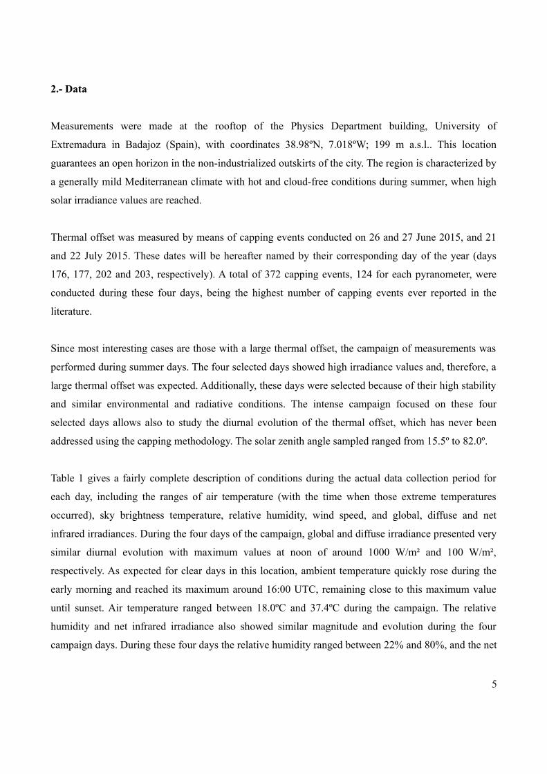
2.- Data

Measurements were made at the rooftop of the Physics Department building, University of

Extremadura in Badajoz (Spain), with coordinates 38.98ºN, 7.018ºW; 199 m a.s.l.. This location

guarantees an open horizon in the non-industrialized outskirts of the city. The region is characterized by

a generally mild Mediterranean climate with hot and cloud-free conditions during summer, when high

solar irradiance values are reached.

Thermal offset was measured by means of capping events conducted on 26 and 27 June 2015, and 21

and 22 July 2015. These dates will be hereafter named by their corresponding day of the year (days

176, 177, 202 and 203, respectively). A total of 372 capping events, 124 for each pyranometer, were

conducted during these four days, being the highest number of capping events ever reported in the

literature.

Since most interesting cases are those with a large thermal offset, the campaign of measurements was

performed during summer days. The four selected days showed high irradiance values and, therefore, a

large thermal offset was expected. Additionally, these days were selected because of their high stability

and similar environmental and radiative conditions. The intense campaign focused on these four

selected days allows also to study the diurnal evolution of the thermal offset, which has never been

addressed using the capping methodology. The solar zenith angle sampled ranged from 15.5º to 82.0º.

Table 1 gives a fairly complete description of conditions during the actual data collection period for

each day, including the ranges of air temperature (with the time when those extreme temperatures

occurred), sky brightness temperature, relative humidity, wind speed, and global, diffuse and net

infrared irradiances. During the four days of the campaign, global and diffuse irradiance presented very

similar diurnal evolution with maximum values at noon of around 1000 W/m² and 100 W/m²,

respectively. As expected for clear days in this location, ambient temperature quickly rose during the

early morning and reached its maximum around 16:00 UTC, remaining close to this maximum value

until sunset. Air temperature ranged between 18.0ºC and 37.4ºC during the campaign. The relative

humidity and net infrared irradiance also showed similar magnitude and evolution during the four

campaign days. During these four days the relative humidity ranged between 22% and 80%, and the net

5

infrared irradiance between -138.0 W/m² and -71.0 W/m². On days 176-177 wind was significantly

different from days 202-203, remaining below 3.2 m/s during days 176 and 177 but reaching values of

up to 6.0 m/s during days 202 and 203. In order to compare days with similar wind conditions, days

176 and 177 were used to study the effect of ventilation on the thermal offset in global irradiance

measurements, and days 202 and 203 to study the effect of mechanical ventilation on the thermal offset

in diffuse irradiance measurements. Thus each pair of days guarantees similar environmental and

radiative conditions. Since moderate winds up to 4.9 and 5.8 m/s were found on days 202 and 203

respectively, the thermal offset in diffuse irradiance is compared between mechanically ventilated and

naturally ventilated by significant winds.

3. Instruments

3.1.- Pyranometers

Three manufacturers lent secondary standard pyranometers with their compatible ventilation units for

the duration of the campaign. They were: 1) a SR20 pyranometer (#3727) with its VU01 ventilation

unit provided by Hukseflux (The Netherlands), 2) a CMP11 pyranometer (#080493) and its CVF4

ventilation unit provided by Kipp & Zonen (The Netherlands), and 3) a SPP pyranometer (#38172)

with its VEN ventilation unit provided by Eppley Laboratories (U.S.A.). These models are widely used

in meteorological stations worldwide.

All the pyranometers used in this study comply with the International Organization for Standardization

ISO 9060 criteria for an ISO secondary standard pyranometer, being classified as ‘‘high quality’’

according to the WMO nomenclature (WMO, 2008). They had been calibrated following standard

WMO procedures according to ISO 9847 (1992). It is to note that this is the first time the thermal offset

of these instruments is simultaneously measured and compared.

The pyranometers studied consist of: 1) a black-coated thermopile acting as a sensor, 2) two concentric

hemispherical domes to protect the sensor, 3) the body or case, which holds the key parts of a

pyranometer, and 4) a sun screen to protect the body and reduce solar heating. Table 2 shows their main

6

characteristics as described in the manufacturers’ instruction manuals and websites (Kipp and Zonen,

2013; Hukseflux, 2014; https://eppleylab.com).

The pyranometer sensors are based on the thermoelectric principle. Although the detector construction

differs between models, the same fundamental working principle is applicable to all of them. The

sensing elements are made up of a large number of thermocouples junction pairs connected in series.

While the reference junction keeps at a fixed temperature, the active junction is exposed to the solar

radiation. Bonded on the active junctions to the thermocouples there is a black-painted ceramic disk

that helps to absorb the incident solar radiation. Blackened thermopile detector is preferred over others

due to its flat spectral response, fast time response and good angular behavior. The temperature of the

active junctions increases when the incoming radiation passes through the two glass domes and is

absorbed by the black ceramic disk. The temperature difference between the active and the reference

junctions produces a small voltage which is a function of the absorbed irradiance.

The sensor is easily affected by environmental factors and the delicate black coating must be protected;

therefore, the sensor is covered by domes. The use of two domes instead of one results in a better

thermal equilibrium between the sensor and the inner dome, therefore reducing the thermal offset. The

pyranometers participating in this study have glass domes with different size: The diameter of the outer

dome is 60 mm in SPP pyranometer, 50 mm in CMP11, and 40 mm in SR20.

The body of a pyranometer is designed to provide high mechanical and thermal stability to the

instrument. The pyranometers participating in the campaign showed differences both in the material

and the design. For example, SR20 and CMP11 have light aluminum bodies while SPP has a heavy

body made of bronze.

There is a screen attached to the body designed to protect it from the rainfall and to reduce solar

heating. The material and design of this screen could play an important role regarding the thermal

offset. On the one hand, it is in contact with the body, therefore affecting the thermal stability. On the

other hand, its size and shape modify the airflow around the pyranometer. Thus, while SR20 and

CMP11 have a screen made of plastic with a diameter of 150 mm, SPP has a flatter screen made of

aluminum with a notably longer diameter of 190 mm.

7

During the campaign the pyranometers were installed on a Kipp & Zonen Solys 2 solar tracker (Figure

1.a.) equipped with shading balls. These balls were only installed on days 202 and 203 in order to

measure diffuse irradiance. Similarly, ventilation units were only installed on days 176 and 203 in order

to obtain measurements under mechanically ventilated conditions. The output signals of the

pyranometers were recorded by a Campbell CR1000 data logger every second.

3.2. Ventilation units

Ventilation units are primarily aimed at preventing dew and frost deposition on the domes which could

disturb the measurements. As a beneficial side effect, ventilation favors the thermal equilibrium

between different parts of a pyranometer, thereby reducing the thermal offset (Kipp and Zonen, 2013;

Hukseflux, 2014).

Three ventilation units participated in our campaign. Their main characteristics are summarized in

Table 3. These ventilation units consist of a base holding a cover and a fan designed to work at 12 volts

DC. Their size, shape and material determine how the air is blown around the body and domes of the

pyranometer, therefore affecting the thermal offset.

The base of the ventilation unit holds the fan and has available space to install the pyranometer. The

ventilation unit bases of our study are made of aluminum, but their sizes and shapes differ. While VEN

and VU01 have a circular base with a diameter of 23.0 cm and 16.5 cm, respectively, the CVF4 has a

circular base of 23.0 cm diameter and an additional branch (Figure 1.b). The shape of the base is

determined by the relative position of the fan with respect to the pyranometer. In VEN and VU01 the

fan is placed under the pyranometer, continuously blowing air upwards over the case and the dome. In

contrast, the CVF4 ventilation unit uses a “squirrel cage” design with the fan located aside the

pyranometer.

The VEN ventilation unit manufactured by Eppley uses a bladed fan which generates an airflow of 85

m³/h. The Huskeflux V01 ventilation unit uses a DC centrifugal fan. The intake of air is in the axial

8

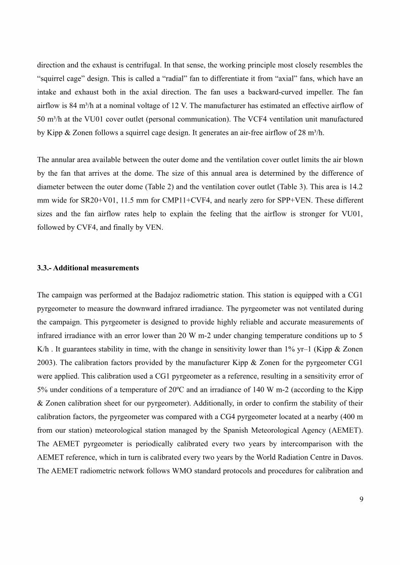
direction and the exhaust is centrifugal. In that sense, the working principle most closely resembles the

“squirrel cage” design. This is called a “radial” fan to differentiate it from “axial” fans, which have an

intake and exhaust both in the axial direction. The fan uses a backward-curved impeller. The fan

airflow is 84 m³/h at a nominal voltage of 12 V. The manufacturer has estimated an effective airflow of

50 m³/h at the VU01 cover outlet (personal communication). The VCF4 ventilation unit manufactured

by Kipp & Zonen follows a squirrel cage design. It generates an air-free airflow of 28 m³/h.

The annular area available between the outer dome and the ventilation cover outlet limits the air blown

by the fan that arrives at the dome. The size of this annual area is determined by the difference of

diameter between the outer dome (Table 2) and the ventilation cover outlet (Table 3). This area is 14.2

mm wide for SR20+V01, 11.5 mm for CMP11+CVF4, and nearly zero for SPP+VEN. These different

sizes and the fan airflow rates help to explain the feeling that the airflow is stronger for VU01,

followed by CVF4, and finally by VEN.

3.3.- Additional measurements

The campaign was performed at the Badajoz radiometric station. This station is equipped with a CG1

pyrgeometer to measure the downward infrared irradiance. The pyrgeometer was not ventilated during

the campaign. This pyrgeometer is designed to provide highly reliable and accurate measurements of

infrared irradiance with an error lower than 20 W m-2 under changing temperature conditions up to 5

K/h . It guarantees stability in time, with the change in sensitivity lower than 1% yr–1 (Kipp & Zonen

2003). The calibration factors provided by the manufacturer Kipp & Zonen for the pyrgeometer CG1

were applied. This calibration used a CG1 pyrgeometer as a reference, resulting in a sensitivity error of

5% under conditions of a temperature of 20ºC and an irradiance of 140 W m-2 (according to the Kipp

& Zonen calibration sheet for our pyrgeometer). Additionally, in order to confirm the stability of their

calibration factors, the pyrgeometer was compared with a CG4 pyrgeometer located at a nearby (400 m

from our station) meteorological station managed by the Spanish Meteorological Agency (AEMET).

The AEMET pyrgeometer is periodically calibrated every two years by intercomparison with the

AEMET reference, which in turn is calibrated every two years by the World Radiation Centre in Davos.

The AEMET radiometric network follows WMO standard protocols and procedures for calibration and

9

measurement, as certified according to ISO 9001:2008. The comparison between our pyrgeometer and

the AEMET pyrgeometer extended over the period August to December 2015, and showed a very good

agreement, with a mean relative difference of 2%.

Figure 2 shows a local time based time series plot of the difference between the pyrgeometer case

temperature (Tcase) and the sky brightness temperature (Tsky). This difference is a descriptor of the

infrared imbalance between the pyrgeometer and the air, which provides interesting information to

understand the thermal offset of the pyranometers. A similar diurnal pattern is found between days 176

and 177, and slightly less similar between days 202 and 203. All days show an increase of the

difference in temperature between the pyrgeometer and the sky along the day. On day 177 the

difference decreases at late evening.

The direct irradiance is measured by a CHP1 pyrheliometer installed on a solar tracker Solys 2, all of

them manufactured by Kipp & Zonen. This pyrheliometer was calibrated in 2013 at the AEMET

Radiometric Laboratory in Madrid, Spain. For this calibration, the Kipp and Zonen CH1 pyrheliometer

#050408, which is directly traced to WRC-Davos, was used as reference. The calibration factor

obtained in this campaign differs in less than 0.1% respect to that provided by the manufacturer.

The station is also equipped with two Kipp and Zonen CM11 pyranometers, one for measuring global

irradiance and the other one, mounted on a CM121 shadow ring, for measuring diffuse irradiance.

These two pyranometers comply with the specifications of the first-class World Meteorological

Organization classification (WMO, 2008) for this instrument. Both pyranometers participated in the

inter-comparison campaign carried out in June 2013 at the “El Arenosillo” Atmospheric Sounding

Station of the National Institute for Aerospace Technology (Huelva, Spain). In this campaign our two

pyranometers were compared to the ventilated Kipp and Zonen CM21 pyranometer #041219 which had

been recently calibrated. The calibration factors obtained in this campaign and the one provided by the

manufacturer notably agree, with relative differences lower than 0.5%, proving the high stability of the

response of both pyranometers.

The diffuse irradiance measurements have been corrected from the shadow ring error according to the

methodology developed by Sanchez et al. (2012).

10

In this station, radiometric data are recorded by a Campbell CR1000 data-logger usually every minute.

However, this study required higher temporal frequency and, therefore, data were recorded every

second during the campaign. These measurements give valuable information about the radiation field

when capping events were being conducted.

Additionally, measurements of ambient temperature, relative humidity and wind speed were registered

every ten minutes at a nearby meteorological station managed by the Spanish Meteorological Agency

(AEMET). This station is only 400 m away from our radiometric station and follows WMO standard

protocols and procedures for calibration and measurement. Wind speed is measured by a THIES

Compact anemometer while ambient temperature and relative humidity are jointly measured by a

THIES Compact probe. Temperature and relative humidity sensors operate inside a Stevenson wooden

shelter to protect against precipitation and direct radiation. The accuracy is ±2% for relative humidity

measurements and ±0.15K for temperature measurements. These measurements describe the

environmental conditions while capping events were being performed.

4.- Methodology

4.1.- Capping events

In this study thermal offset measurements have been obtained following the capping methodology. This

technique consists of recording the pyranometer output signal while the incoming solar radiation is

blocked by a cap that covers the dome. When no solar radiation arrives at the sensor, the output signal

is a measure of the exchange of infrared flux between the dome and the sensor, that is, the thermal

offset. The capping event should last until the detector has responded to the blocking of shortwave

radiation, but it should be short enough to prevent significant changes in the temperature of the dome.

It must be noted that this study has performed the highest number of capping events ever reported in

the literature. In fact they are many more than the measurements reported in the previous studies that

have used the same methodology, such as in Haeffelin (2001), Michalsky (2003), Michalsky (2005),

11

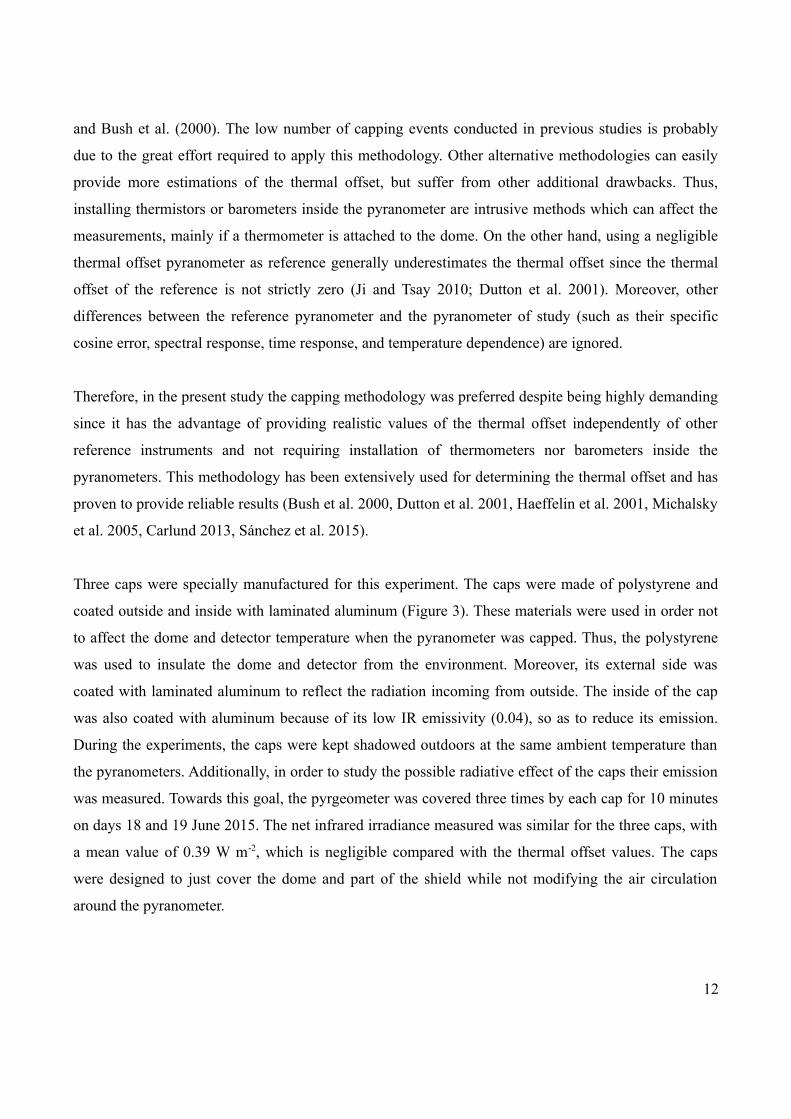
and Bush et al. (2000). The low number of capping events conducted in previous studies is probably

due to the great effort required to apply this methodology. Other alternative methodologies can easily

provide more estimations of the thermal offset, but suffer from other additional drawbacks. Thus,

installing thermistors or barometers inside the pyranometer are intrusive methods which can affect the

measurements, mainly if a thermometer is attached to the dome. On the other hand, using a negligible

thermal offset pyranometer as reference generally underestimates the thermal offset since the thermal

offset of the reference is not strictly zero (Ji and Tsay 2010; Dutton et al. 2001). Moreover, other

differences between the reference pyranometer and the pyranometer of study (such as their specific

cosine error, spectral response, time response, and temperature dependence) are ignored.

Therefore, in the present study the capping methodology was preferred despite being highly demanding

since it has the advantage of providing realistic values of the thermal offset independently of other

reference instruments and not requiring installation of thermometers nor barometers inside the

pyranometers. This methodology has been extensively used for determining the thermal offset and has

proven to provide reliable results (Bush et al. 2000, Dutton et al. 2001, Haeffelin et al. 2001, Michalsky

et al. 2005, Carlund 2013, Sánchez et al. 2015).

Three caps were specially manufactured for this experiment. The caps were made of polystyrene and

coated outside and inside with laminated aluminum (Figure 3). These materials were used in order not

to affect the dome and detector temperature when the pyranometer was capped. Thus, the polystyrene

was used to insulate the dome and detector from the environment. Moreover, its external side was

coated with laminated aluminum to reflect the radiation incoming from outside. The inside of the cap

was also coated with aluminum because of its low IR emissivity (0.04), so as to reduce its emission.

During the experiments, the caps were kept shadowed outdoors at the same ambient temperature than

the pyranometers. Additionally, in order to study the possible radiative effect of the caps their emission

was measured. Towards this goal, the pyrgeometer was covered three times by each cap for 10 minutes

on days 18 and 19 June 2015. The net infrared irradiance measured was similar for the three caps, with

a mean value of 0.39 W m-2, which is negligible compared with the thermal offset values. The caps

were designed to just cover the dome and part of the shield while not modifying the air circulation

around the pyranometer.

12

Previous studies have shown that once the pyranometer is covered, the output signal decreases, reaches

a minimum and then smoothly increases to approach a stable value (Bush et al. 2000; Sanchez et al.

2015). In the current study the thermal offset was obtained as the minimum value reached by the signal

during the capping event, as it was suggested by Bush et al. (2000). This criterion compares well with

other estimations (Sanchez et al., 2015) while requiring no estimation of the time constant of the

pyranometer, which can be difficult to determine.

In order to analyze the evolution of the output signal when the pyranometer is covered, preliminary

long capping events were carried out. Six long capping events were conducted with each pyranometer,

three of them with mechanical ventilation and other three without mechanical ventilation. As a result of

the information obtained from the preliminary measurements, following capping events were decided

to last five minutes. The capping events were performed approximately every 40 minutes to prevent

memory effects from happening. The three pyranometers were covered simultaneously to guarantee the

measurements were performed under the same environmental conditions.

4.2.- Analysis

Previous studies have reported relationships between thermal offset and environmental variables (Bush

et al. 2000; Haeffelin et al. 2001; Dutton et al. 2001; Sanchez et al., 2015). Among the main factors

affecting the thermal offset, several authors pointed out the role played by the infrared downward

irradiance at ground level. An increase of downward IR irradiance heats the dome and consequently

reduces the difference in temperature between the dome and the detector. Several authors have

quantified this influence using Net IR as measured by a pyrgeometer and/or the difference of

temperature between the pyrgeometer case and the sky brightness temperature (Dutton et al.

2001;Haeffelin et al. 2001; Younkin and Long, 2004; Michalsky et al. 2005; Gueymard and Myers

2009).

Additionally, the thermal offset is affected by the ambient temperature (Ta), relative humidity (RH) and

wind speed (W) (Bush et al. 2000; Dutton et al. 2001; Haeffelin et al. 2001; Philipona 2002; Michalsky

et al., 2003; Sanchez et al. 2015). The impact of these factors on thermal offset will mainly depend on

the pyranometer design. For example, the wind affects both the dome and body but, while the dome is

13

completely exposed, the body is partially protected by the pyranometer sun screen.

The dependence of daytime thermal offset on these environmental variables and the influence of

mechanical ventilation have been thoroughly evaluated for the three pyranometers participating in the

campaign.

Additionally, the performance of the model proposed by Dutton et al. (2001) to correct the thermal

offset was evaluated. This model proposes a relationship between the thermal offset of a pyranometer

and the net infrared irradiance measured by a collocated pyrgeometer, Net IR, as follows:

(1)

According to the Dutton et al.’s proposal, the coefficient b is estimated using nighttime measurements

and the obtained model is applied to correct the daytime thermal offset. The Dutton et al.’s method is

intended to use the pyrgeometer as a tracer of the pyranometer. Therefore, in order to most accurately

mimic the conditions that the pyranometer is experiencing, they both must operate under the same

ventilation conditions. Since the pyrgeometer used in this study was unventilated, the analysis is only

applied to measurements registered by unventilated pyranometers. Nighttime data were selected as

those measurements registered when solar altitude was below -10º during nights 177 and 202 (no

ventilation was applied).

Ordinary linear least square fittings have been obtained for each pyranometer and the coefficient of

determination R² was calculated to quantify the goodness-of-fit. This statistic measures how well the

observed outcomes are replicated by the model. Additionally, fittings with the intercept forced through

(0,0) have also been analyzed. This is a common practice since a zero offset is expected when Net IR

equals zero, i.e., when the dome and the sensor of the pyrgeometer have the same temperature.

Afterwards, the nighttime-fitted model was employed to estimate the diurnal thermal offset. The

differences between modeled and measured thermal offset values will be analyzed for unventilated

pyranometers while measuring global or diffuse irradiance.

14

5.- Results and discussion

Section (5.1) shows the results of preliminary capping events. In section 5.2, the daytime thermal offset

measured for each pyranometer and operational configuration is analyzed. Next, the relationship

between the thermal offset and several environmental factors is discussed (Section 5.3). Finally, the

performance of the Dutton et al.’s model to correct the daytime thermal offset is evaluated (Section

5.4). It should be noticed that, as offsets are usually negative, a reference to increasing offset means

more negative and vice versa.

5.1.- Preliminary capping events

Figure 4.a shows an example of the output signal measured by each pyranometer during a preliminary

capping event conducted without mechanical ventilation. Vertical lines are plotted to highlight the time

that each pyranometer takes to reach its thermal offset.

In all these six preliminary long capping events, the unventilated CMP11 pyranometer shows a sharp

minimum with a well-defined thermal offset, taking a mean time of 10.1 s (standard deviation is 1.5 s)

to reach the minimum. Meanwhile, the unventilated SPP and SR20 pyranometers requiring a mean time

of 33.2 s (standard deviation is 5.9 s) and 63.8 s (standard deviation is 10.0 s) to reach their respective

minimum values, taking several seconds to start increasing again.

Figure 4.b. shows an example of the evolution of the output signal measured by each pyranometer

during a preliminary capping event while applying ventilation. The time needed by the CMP11 and

SPP pyranometers to reach their minimum signal was similar to the values corresponding to the

unventilated case. On the contrary, the time needed by SR20 pyranometer notably increases when it is

mechanically ventilated. The average time taken by this instrument to reach its minimum value while

being ventilated was 150.5 s (with a standard deviation of 18.8 s). This long period of time could

significantly affect the estimation of the thermal offset: the temperature of the dome could decrease,

causing an underestimation of the thermal offset prior to the capping. In spite of this behavior, the

ventilated SR20 has been included in this study; however, its results should be taken with caution.

15

5.2. Thermal offset measurements

5.2.1. Thermal offset for unventilated pyranometers while measuring global irradiance (UG)

Figure 5.a shows the thermal offset values measured on day 177 by unventilated pyranometers

measuring global irradiance. All pyranometers show a clear diurnal cycle, being more pronounced for

the CMP11. This diurnal pattern shows three stages: 1) at early morning hours the absolute thermal

offset clearly increases (becomes more negative), 2) between mid-morning and around 17:00 UTC the

thermal offset oscillates around a constant value, and 3) afterwards the absolute thermal offset

decreases (becomes less negative). A similar pattern has been previously reported for two CM11

pyranometers by Sanchez et al. (2015), who suggested that this behaviour during cloudless summer

days could be explained by the diurnal variation in the direct/diffuse partitioning.

The mean value of the UG measurements registered during the central period of day 177 is around

-6.85W/m² (standard deviation of 2.0W/m²) for the SPP and SR20 pyranometers, but reaches

-15.0W/m² for the CMP11 pyranometer. These values fall in the range of thermal offset derived by

Bush et al. (2000) for an unventilated PSP measuring global irradiance under cloudless skies. They

estimated the thermal offset using measurements of the temperature of the dome and the body,

obtaining values between -17.0 W/m² and -6.5 W/m². It must be noted that, although unventilated

CMP11 shows the highest absolute thermal offset (most negative), it is very stable during the central

hours of the day, with the standard deviation being 1.0W/m² .

5.2.2. Thermal offset for ventilated pyranometers while measuring global irradiance (VG)

Figure 5.b shows the thermal offset measured on day 176 by mechanically ventilated pyranometers

measuring global irradiance. The main difference with respect to the unventilated case is the removal of

the diurnal cycle. Instead, the VG for SR20 oscillates around -4.5 W/m² all day long. The absolute

value of the VG for the CMP11 slightly rises from the early morning to around 15:00 UTC and then,

vaguely decreases until the sunset. Meanwhile, the absolute values of the thermal offset for the

ventilated SPP pyranometer slightly decreases during the day.

There is a significant reduction in the absolute value of thermal offset when the pyranometers are

16

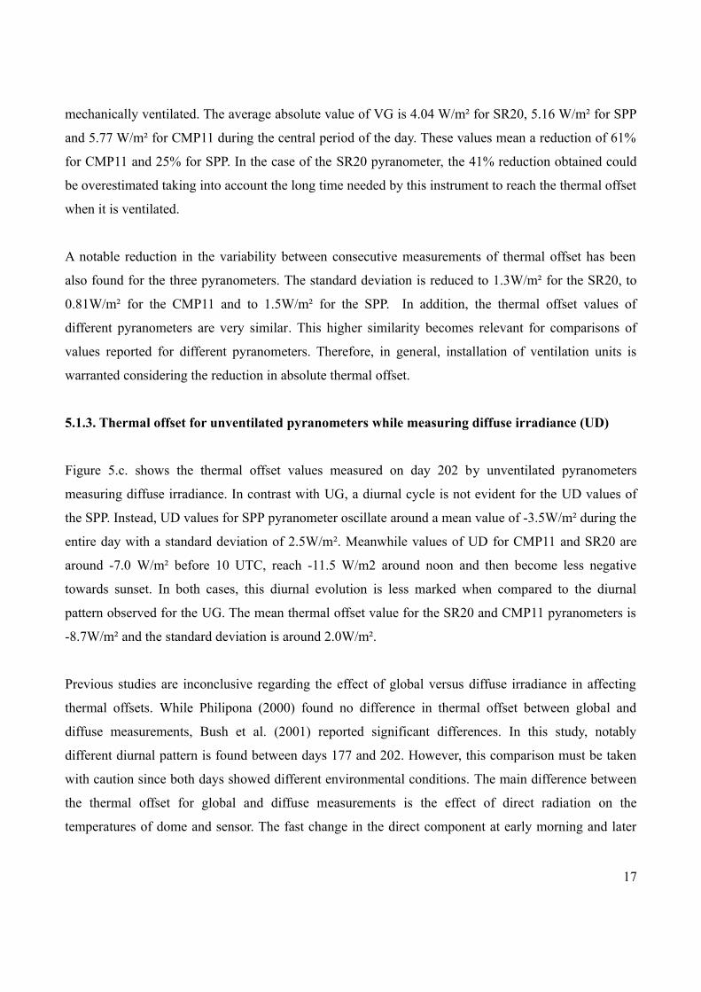
mechanically ventilated. The average absolute value of VG is 4.04 W/m² for SR20, 5.16 W/m² for SPP

and 5.77 W/m² for CMP11 during the central period of the day. These values mean a reduction of 61%

for CMP11 and 25% for SPP. In the case of the SR20 pyranometer, the 41% reduction obtained could

be overestimated taking into account the long time needed by this instrument to reach the thermal offset

when it is ventilated.

A notable reduction in the variability between consecutive measurements of thermal offset has been

also found for the three pyranometers. The standard deviation is reduced to 1.3W/m² for the SR20, to

0.81W/m² for the CMP11 and to 1.5W/m² for the SPP. In addition, the thermal offset values of

different pyranometers are very similar. This higher similarity becomes relevant for comparisons of

values reported for different pyranometers. Therefore, in general, installation of ventilation units is

warranted considering the reduction in absolute thermal offset.

5.1.3. Thermal offset for unventilated pyranometers while measuring diffuse irradiance (UD)

Figure 5.c. shows the thermal offset values measured on day 202 by unventilated pyranometers

measuring diffuse irradiance. In contrast with UG, a diurnal cycle is not evident for the UD values of

the SPP. Instead, UD values for SPP pyranometer oscillate around a mean value of -3.5W/m² during the

entire day with a standard deviation of 2.5W/m². Meanwhile values of UD for CMP11 and SR20 are

around -7.0 W/m² before 10 UTC, reach -11.5 W/m2 around noon and then become less negative

towards sunset. In both cases, this diurnal evolution is less marked when compared to the diurnal

pattern observed for the UG. The mean thermal offset value for the SR20 and CMP11 pyranometers is

-8.7W/m² and the standard deviation is around 2.0W/m².

Previous studies are inconclusive regarding the effect of global versus diffuse irradiance in affecting

thermal offsets. While Philipona (2000) found no difference in thermal offset between global and

diffuse measurements, Bush et al. (2001) reported significant differences. In this study, notably

different diurnal pattern is found between days 177 and 202. However, this comparison must be taken

with caution since both days showed different environmental conditions. The main difference between

the thermal offset for global and diffuse measurements is the effect of direct radiation on the

temperatures of dome and sensor. The fast change in the direct component at early morning and later

17

evening could be the main factor determining the increase and decrease in UG. In the absence of direct

irradiance in unventilated diffuse measurements, this tendency disappears in the morning and is

smoother during the afternoon. This result about the effect of the direct/diffuse partitioning on the

thermal offset tends to agree with several studies (Bush, 2000; Cess, 2000; Sanchez et al., 2015).

However, opposite conclusions have been also reported (Younkin and Long, 2004; Vignola et al., 2007,

2008, 2009; Philipona, 2002) and the issue remains controversial. This diversity in results is probably

related to the distinct methodology, instrumentation, and location used in the different studies. Thus,

further analysis are needed to assess possible differences in the thermal offset of pyranometers

depending on whether they are measuring global or diffuse irradiance.

Most UD values obtained for the three pyranometers are less negative than the value -20W/m² given by

Haeffelin et al. (2001) for a PSP pyranometer or the value -11.0W/m² reported by Dutton et al. (2001)

for two CM21 pyranometers.

5.2.4. Thermal offset for ventilated pyranometers while measuring diffuse irradiance (VD)

Figure 5.d shows the thermal offset measured on day 203 by mechanically ventilated pyranometers

measuring diffuse irradiance. Ventilation affects the thermal offset of diffuse irradiance measurements

similarly than it was observed for global irradiance measurements. One of its most noticeable effects is

the reduction in the variability between consecutive measurements of the thermal offset for all the

pyranometers.

The thermal offset of the SR20 pyranometer oscillates around a mean value of -6.17W/m² during the

day, with a standard deviation of 1.1W/m². However, this value could be higher considering the time

needed by this instruments to reach the minimum when it is covered. In the case of the CMP11

pyranometer, the absolute value of the thermal offset rises from the early morning to around 14:00

UTC and then, decreases towards sunset. This pyranometer shows the largest reduction in the absolute

thermal offset with a mean value of 3.4W/m² and a standard deviation of 2.0W/m². A decrease of

around 50% in the maximum VD has been observed for the CMP11 with respect to that obtained when

it was measuring UD. At the same time, a clear tendency is detected in VD for the SPP pyranometer.

The absolute thermal offset of this pyranometer increases smoothly during the day and reaches a

18

maximum value of 9.0 W/m² during sunset. Its mean value for that day is 4.4W/m² and the standard

deviation 2.5W/m². A possible explanation for this increase could be the small outlet of the ventilation

unit, that allows no airflow supplied by the fan to reach the dome. With this design, the air driven by

the fan circulates only around the body, while the dome is exposed to natural air circulation and to the

environmental conditions. The effect of the artificial ventilation on the thermal offset dependence on

the environmental conditions will be thoroughly analyzed in the next section. The CMP11 and SPP

pyranometers showed similar VD patterns than those observed for VG. This issue will be analyzed in

the next section.

Other studies have obtained experimental VD values on cloudless skies by means of capping events

(Dutton et al., 2001; Haeffelin et al., 2001; Michalsky et al., 2003). Haeffelin et al. (2001) and Dutton

et al. (2001) reported thermal offset values between -15 and -5 W/m² for a PSP pyranometer. These

values differ from the results obtained in this study for the CMP11, SPP and SR20 pyranometers. These

differences between pyranometer models emphasize the need to individually characterize each

instrument and the environmental conditions surrounding each experiment.

5.3. Effect of mechanical ventilation on the influence of environmental conditions

Mechanical ventilation modifies the air circulation around the pyranometers, particularly, around the

body and the dome. This change could directly affect the thermal offset and its relationship with the

natural environmental conditions. In this section, the effect of ventilation on the relationship between

the thermal offset and the environmental variables is examined. To assess these relationships,

regression models between the thermal offset of each pyranometer and each independent variable were

fitted using the least squares approach.

Figure 6 depicts the behavior of the thermal offset values vs wind speed (W), ambient temperature (Ta),

relative humidity (RH), net infrared irradiance (Net IR) and the difference between the pyrgeometer

case temperature and the sky brightness temperature (Tcase-Tsky). Data when the pyranometers were

measuring global irradiance with and without mechanical ventilation are shown.

The thermal offset in the unventilated CMP11 pyranometer measuring global irradiance shows a

19

positive tendency with respect to the Net IR irradiance (with R² = 0.713) and relative humidity (with R²

= 0.475). It shows a negative tendency with respect to ambient air temperature (with R² = 0.5) as

expected, since relative humidity and air temperature are anticorrelated. This behavior agrees with the

behavior observed by Serrano et al. (2015) for two unventilated CM11. Similarly, a negative tendency

with respect to the Tcase-Tsky difference is expected since this variable is anticorrelated with the Net

IR. These tendencies are however less evident for the SPP (with R² below 0.43), and imperceptible for

the SR20 (with R² values below 0.22).

When the pyranometers are measuring global irradiance while being ventilated (grey points in Figure

6) the decrease in the thermal offset described in Section 5.1.b is confirmed. While SR20 shows no

clear patterns (with R² below 0.38), the CMP11 and SPP pyranometers show similar tendencies to those

observed for unventilated measurements (UG), but notably smoother. The CMP11 pyranometer shows

the largest attenuation of these tendencies due to ventilation. In general, it is observed that the air

generated by the fan seems to homogenize the conditions around the pyranometer favoring the

reduction of the thermal offset and its dependence on the environmental conditions.

The persistence of the trends on the CMP11 and SR20 when these two pyranometers are ventilated

could be likely related to the actual air volume rate out of their corresponding ventilation units. There

are many factors involved in the actual amount of ventilation finally flow around the dome, such as the

fan volume and type (bladed/squirrel/radial) and its design. As it was described in Section 3.2., the

SR20-VU01 has a fan with a very high volume rate, and a large annular area between the dome and the

ventilation cover outlet. Conversely, CMP11-CVF4 and SPP-VEN have lower volume rate fans, and

the annular areas available for the airflow to reach the dome are notably smaller.

Figure 7 shows the thermal offset vs wind speed (W), ambient temperature (T), relative humidity (RH)

and net infrared irradiance (Net IR) when the pyranometers were measuring diffuse irradiance with and

without ventilation. One of the most important results observed for UD is the lack of tendencies with

respect to the environmental variables being analyzed, with R² being below 0.22 for all pyranometers.

A certain diurnal pattern is only observed for the CMP11 pyranometer. This result confirms the

importance of the direct/diffuse partitioning on the daily thermal offset behaviour as suggested in

Section 5.1.c.

20

The SR20 pyranometer shows no clear tendency respect to any environmental variable while

measuring diffuse irradiance and being ventilated (R² below 0.10). On the contrary, the CMP11 and

SPP pyranometers show marked relationships with respect to several environmental variables. The

thermal offset of diffuse irradiance measurements tends to increase with wind speed, ambient

temperature and Tc-Ts difference, and to decrease with Net IR irradiance and relative humidity when

the pyranometers are ventilated.

5.4.- Thermal offset correction obtained from nighttime data

5.4.a.- Nighttime fittings

Nighttime thermal offset vs the Net IR values and its corresponding linear least squares fit (solid grey

line) are shown in Figure 8 for each pyranometer. The fittings coefficients are summarized in Table 4

together with the root-mean-squared-error (RMSE) and the coefficient of determination (R²).

The SPP pyranometer shows a slope of 0.0337, which is similar to the values reported by Haeffelin

(2001) and Michalsky (2005) for a ventilated PSP. However, the coefficient of determination R² is

below 0.16 in all cases, indicating that most of the variance is not explained by the linear model.

Several authors have previously reported no trend between the nighttime offset and Net IR (Michalsky

et al., 2003; Michalsky et al., 2005; Gueymard, 2009). In our particular case, it is difficult to conclude

this since the low significance of the fitting could be likely due to the lack of cases with small values of

Net IR during the analyzed nights.

In usual practice, the intercept is forced through (0,0) since a zero offset is expected when Net IR

equals zero, i.e., when the dome and the sensor of the pyrgeometer are at the same temperature. The no-

intercept regression line for each pyranometer has been plotted as a dashed black line in Figure 8.

The slopes obtained for the no-intercept fittings are 0.01 for the SR20 pyranometer, and 0.04 for the

CMP11 and SPP pyranometers. All regression coefficients were statistically significant at 95% level of

confidence. Dropping the intercept results in a small change in the fitting for SPP since it was the one

to show the smallest intercept in the non-forced-to-zero fitting. The CMP11 fitting gets closer to the

21

SPP fitting when the intercept is forced to be zero.

5.4.b.- Application to correct the daytime thermal offset

The zero-intercept regression models obtained in the previous section were applied to daytime Net IR

irradiance measurements and the resulting daytime thermal offset was compared to the experimental

values measured using capping events. Figure 9 shows the absolute differences found between the

modeled and the measured daytime thermal offset values for days 177 (UG) and 202 (UD).

It can be observed that Dutton et al.’s model notably underestimates the absolute value of the daytime

thermal offset for the SR20 and CMP11 pyranometers. This underestimation is larger when the CMP11

pyranometer measures global irradiance than when it is shadowed, and it shows a marked relationship

with the solar zenith angle. A similar pattern was reported by Vignola et al. (2007) when measuring

diffuse irradiance with a PSP pyranometer while being ventilated.

The regression model obtained with nighttime data performs better for the SPP pyranometer, with

absolute differences between modeled and measured values being lower than 5 W/m² and almost

uniformly scattered around the zero line. Thus, although our results apply to unventilated

pyranometers, these results for the SPP pyranometer are in line with the widely application of Dutton et

al.’s model for the ventilated PSP pyranometer, manufactured also by Eppley.

The previous studies that apply the Dutton et al.’s model mainly focussed on diffuse irradiance

measurements (Dutton et al., 2001; Michalsky et al., 2005 and 2007). They have reported differences in

the daytime thermal offset between model and capping-event measurements of around 1.5 W/m² for

ventilated pyranometers and 7 W/m² for unventilated pyranometers. Thus, our results for SPP and

SR20 pyranometers fall within the expected range. On the other hand, the CMP11 pyranometer shows

somewhat larger differences up to 11 W/m², and notable differences between global and diffuse

measurements are found as well.

22

6.- Conclusions

An intensive campaign to assess the effect of artificial ventilation on the thermal offset of pyranometers

was carried out during selected cloudless days in June and July 2015 in Badajoz (Spain). The SR20

(Hukseflux), CMP11 (Kipp & Zonen) and SPP (Eppley) secondary standard pyranometers with their

corresponding VU01, CVF4 and VEN ventilation units participated in this campaign. Daytime thermal

offset was experimentally measured by means of capping events for each pyranometer while measuring

global or diffuse irradiance, and with and without ventilation. To our knowledge, this is the first study

to measure and compare the thermal offset of the CMP11, SPP and SR20 pyranometers, on such

configurations and in actual field conditions.

Preliminary measurements revealed limitations to apply the capping methodology to the SR20

pyranometer while being ventilated. In this configuration the output signal takes 150s to reach the

minimum once the pyranometer is capped. This long period of time could significantly affect the

temperature of the dome, resulting in an underestimation of the thermal offset prior to its capping.

The comparison between unventilated and ventilated thermal offset when the pyranometers are

measuring global or diffuse irradiance shows interesting results. Generally, mechanical ventilation

tends to homogenize the temperature between the sensor and the domes and, therefore, to reduce the

thermal offset. Additionally, a notable decrease in the short-term variability of the thermal offset was

detected when the pyranometers were ventilated.

Results obtained in this study confirm the differences in the thermal offset between different

pyranometer models as reported by previous studies (Dutton et al., 2001; Michalsky et al., 2003) but

also reveal notable disparities in their daytime behavior. These differences between pyranometer

models are generally reduced when mechanical ventilation is applied. This homogenization of the

thermal offset becomes relevant for the comparison of different pyranometers.

In order to correct the daytime thermal offset, several authors have suggested mathematical expressions

based on environmental variables (Vignola et al., 2007, 2008, 2009; Dutton et al., 2001; Serrano et al.,

2015). Along these lines, the present study shows important differences in the relationships with

23

environmental magnitudes depending on whether the pyranometer is ventilated or not. The tendencies

detected for the CMP11 and SPP pyranometers while ventilated could be related to the small size of the

outlet of the ventilation unit, which hinders the airflow to reach the dome.

Additionally, the correction model proposed by Dutton et al. (2001) was essayed in this study. The

relationship between the nighttime thermal offset and the Net IR irradiance was analyzed for each

pyranometer under unventilated conditions. No significant relationship were found (R² below 0.16 for

all regression fittings), being in line with other authors (Michalsky et al., 2003; Gueymard and Myers,

2009). However, the low significance could be also related to the lack of cases with Net IR values close

to zero. Additionally, regression models forced through (0,0) were also fitted to nighttime data. Then,

the fitted models were applied to estimate the daytime thermal offset. Differences between modeled

and measured daytime values indicated that Dutton et al.’s model performs well for the unventilated

SPP but it is unsuitable for CMP11 and SR20.

The analysis performed in this study highly recommends the general use of ventilation units. However,

it must be emphasized that each pyranometer model must be individually studied with its ventilation

unit under actual working conditions.

This study aims to contribute to a better knowledge of the thermal offset error in pyranometers,

focusing on the effect of ventilation. The methodology and comparisons described in this paper can be

applied at other locations, with other instruments and environmental conditions. The findings can be

specially relevant for long-term historical radiation series recorded worldwide by networks such as

BSRN, GEBA, SAURAN, SMN-AWS, etc. The reduction in the thermal offset when mechanical

ventilation is applied has been quantified to be between 1.3 W/m² and 9 W/m². This value is in the

order of the general changes in global radiation occurred during the 1960–1990 dimming period

(variation between -5.1 and -1.6 W m-2 decade-1) and the later brightening period (variation between

+2.2 and +5.1 W m-2 decade-1) (Wild et al., 2009). And also similar to the trend (+3 W m-2 decade-1) in

the diffuse irradiance in USA for the period 1996-2007 reported by Long et al. (2009), and to the trend

(-1.3W m-2 decade-1) in Girona (Spain) for the period 1994-2014 recently reported by Calbo et al.

(2016). Thus, neglecting the thermal offset error could hinder the detection of these long trends, and the

mechanical ventilation has been revealed in this study as an efficient method to reduce such error.

24

This study also suggests directions for future research concerning the development of models to correct

the daytime thermal offset based on environmental and radiative magnitudes. It would be useful in

further work to assess offset and ventilation characteristics with instruments of the same type. This

might provide some general relationships typical of the pyranometer model.

7.- Acknowledgements

This study was partially supported by the research projects CGL2011-29921-C02-01 and CGL2014-

56255-C2-1-R granted by the Ministerio de Economía y Competitividad from Spain and by Ayuda a

Grupos GR15137 granted by Junta de Extremadura and Fondo Social Europeo (FEDER). Authors

thank to Eppley, Hukseflux and Kipp & Zonen for providing their instrument to this study and to the

Spanish Agencia Estatal de Meteorología (AEMet) for the provision of meteorological data. Guadalupe

Sanchez Hernandez thanks the Ministerio de Economía y Competitividad for the predoctoral FPI grant

BES-2012-054975. The data analyzed in this study are available from authors upon request

([email protected]).

8.- References

Bush, B.C., F.P.J. Valero, and A.S. Simpson, 2000: Characterization of thermal effects in pyranometers:

A data correction algorithm for improved measurement of surface insolation. J. Atmos. Oceanic

Technol., 17, 165-175.

Calbó, J., González, JA. & Sanchez-Lorenzo, A. (2016), Building global and diffuse solar radiation

series and assessing decadal trends in Girona (NE Iberian Peninsula). Theor Appl Climatol (2016).

doi:10.1007/s00704-016-1829-3

Cess, R.D., Q. Taotao, S. Moguo, 2000: Consistency tests applied to the measurement of total, direct,

and diffuse shortwave radiation at the surface, Journal of Geophysical Research: Atmospheres, 105,

D20, doi:10.1029/2000JD900402.

25

Carlund T., 2013: Baltic Region Pyrheliometer Comparison 2012. World Meteorological Organization,

Rep. 112, pp. 10-35, Geneva, Switzerland.

Dutton, E.G., J.J. Michalsky, T. Stoffel, B.W. Forgan, J. Hickey, D.W. Nelson, T.L. Alberta, and I.

Reda, 2001: Measurement of broadband diffuse solar irradiance using current commercial

instrumentation with a correction for thermal offset errors. J. Atmos. Oceanic Technol., 18, 297-314.

https://eppleylab.com

Gu, L. H., D. D. Baldocchi, S. C. Wofsy, J. W. Muger, J. j. Michalsky, S. P. Urbanski, T. A. Boden,

2003: Response of a deciduous forest to the Mount Pinatubo eruption: enhanced photosynthesis,

Science, 299, 2035-2038.

Gueymard CA, Myers DR (2009) Evaluation of conventional and high-performance routine solar

radiation measurements for improved solar resource, climatological trends, and radiative modeling. Sol

Energy 83:171–185

Haeffelin, M., S. Kato, A.M. Smith, C.K. Rutledge, T.P. Charlock, and J.R. Mahan, 2001:

Determination of the thermal offset of the Eppley precision spectral pyranometer. Applied Optics, 4,

472-484.

Hukseflux, 2014; User manual SR20 secondary standard pyranometer. Manual v1407.

International Organization for Standardization (ISO) 9060, 1990: Solar energy -- Specification and

classification of instruments for measuring hemispherical solar and direct solar radiation.

International Organization for Standardization (ISO) 9847, 1992 :Solar energy -- Calibration of field

pyranometers by comparison to a reference pyranometer.

Ji, Q., 2007: A method to correct the thermal dome effect of pyranometers in selected historical solar

irradiance measurements, Journal of Atmospheric and Oceanic Technology, 24, 529-536.

26

Kipp & Zonen, 2013: Instruction manual CMP series pyranometers and CMA series albedometers.

Long, C. N., and Y. Shi (2008), An automated quality assessment and control algorithm for surface

radiation measurements, Open Atmos. Sci. J. ,2, 23–37, doi:10.2174/1874282300802010023

Long, C.N., E.G. Dutton, J. A. Augustine, W. Wiscombe, M. Wild, S. A. McFarlane, and C. J. Flynn,

2009: Significant decadal brightening of downwelling shortwave in the continental United States, J.

Geophys. Res., 114, D00D06, doi: 10.1029/2008JD011263.

Michalsky, J.J., R. Dolce, E.G. Dutton, M. Haeffelin, G. Major, J.A. Schlemmer, D.W. Slater, J.

Hickey, W. Q. Jeffries, A. Los, D. Mathias, L.J.B. McArthur, R. Philipona, I.Reda, and T. Stoffel,

2003: Results from the first ARM diffuse horizontal shortwave irradiance comparison, J. Geophys.

Res., 108, 4108, doi:10.1029/2002JD002825.

Michalsky, J. J., et al. (2005), Toward the development of a diffuse horizontal shortwave irradiance

working standard, J. Geophys. Res., 110, D06107, doi:10.1029/2004JD005265.

Philipona, R., 2002: Underestimation of solar global and diffuse radiation measured at Earth's surface.

J. Geophys. Res., 107, 4654, doi: 10.1029/2002JD002396.

Reda, I., T. Stoffel and D. Myers, 2003: A method to calibrate a solar pyranometer for measuring

reference diffuse irradiance. Sol. Ener., 74, 103-112.

Roderick, M. L., G. D. Farquhar, S. L. Berry, and I. R. Noble, 2001: On the direct effect of clouds and

atmospheric particles on the productivity and structure of vegetation, Oecologia, 129, 21-30.

Sanchez, G., A. Serrano, M.L. Cancillo, and J.A. Garcia, 2015: Pyranometer thermal offset:

Measurement and analysis. J. Atmos. and Oceanic Tech., 32, 234-246. doi: 10.1175/JTECH-D-14-

00082.1

27

Serrano, A., Sanchez, G., & Cancillo, M. L., 2015: Correcting daytime thermal offset in unventilated

pyranometers. Journal of Atmospheric and Oceanic Technology, 32, 2088 - 2099.

Vignola F, C.N. Long, and I Reda. 2007. Evaluation of Methods to Correct for IR Loss in Eppley PSP

Diffuse Measurements. Optical Modeling and Measurements for Solar Energy Systems Proceedings

Volume 6652, DR Meyers, ed. DOI: 10.1117/12.734474.

Vignola, F., C. Long, I. Reda, 2008: Modeling IR Radiative Loss from Eppley PSP Pyranometers.

Proceeding in Society of Photo-Optical Instrumentation Engineers (SPIE) conference, San Diego,

California.

Vignola, F., C. Long, I. Reda, 2009: Testing a model of IR radiative losses. Proceeding in Society of

Photo-Optical Instrumentation Engineers (SPIE) conference, San Diego, California, NREL.

Wild M., 2009: Global dimming and brightening: a review. J. Geophys. Res., 114, doi:

10.1029/2008JD011470.

Wild, M., 2012: Enlightening global dimming and brightening. Bull. Am. Meteorol. Soc., 93, 27-37.

28

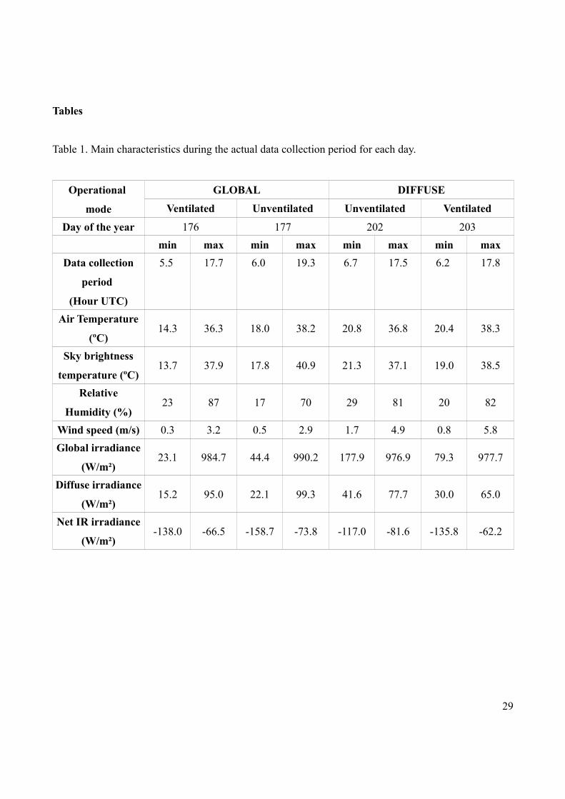
Tables

Table 1. Main characteristics during the actual data collection period for each day.

Operational

mode

GLOBAL DIFFUSE

Ventilated Unventilated Unventilated Ventilated

Day of the year 176 177 202 203

min max min max min max min max

Data collection

period

(Hour UTC)

5.5 17.7 6.0 19.3 6.7 17.5 6.2 17.8

Air Temperature

(ºC)14.3 36.3 18.0 38.2 20.8 36.8 20.4 38.3

Sky brightness

temperature (ºC)13.7 37.9 17.8 40.9 21.3 37.1 19.0 38.5

Relative

Humidity (%)23 87 17 70 29 81 20 82

Wind speed (m/s) 0.3 3.2 0.5 2.9 1.7 4.9 0.8 5.8

Global irradiance

(W/m²)23.1 984.7 44.4 990.2 177.9 976.9 79.3 977.7

Diffuse irradiance

(W/m²)15.2 95.0 22.1 99.3 41.6 77.7 30.0 65.0

Net IR irradiance

(W/m²)-138.0 -66.5 -158.7 -73.8 -117.0 -81.6 -135.8 -62.2

29

Table 2. Main characteristics of the participating pyranometers provided by the manufacturers in their

corresponding manuals and websites. Thermal offset in this table is commonly denominated as “Offset

A” in pyranometer manuals.

Model SPP SR20 CMP11

Manufacturer Eppley Hukseflux Kipp & Zonen

Serial number 38172 3727 080493

Spectral range (nm)

(50% points)295-2800 285-3000* 285-2800

Dome material glass glass glass

Body material bronze aluminum aluminum

Shield material aluminum aluminum plastic

Outer dome

diameter (mm)50 40 50

Unventilated

Offset A (W/m²)5 5 <7

Ventilated

Offset A(W/m²)-- 2.5 50% reduction

* Spectral range for 20% transmision points

30

Table 3. Main characteristics of the ventilation units provided by the manufacturers in their

corresponding manuals and websites .

Ventilation Unit VEN VU01 CVF4

Manufacturer Eppley Hukseflux Kipp & Zonen

Pyranometer SPP SR20 CMP11

Base Material aluminium aluminium aluminium

Cover material plastic+aluminum aluminum plastic

Dimensions

(base diameter (cm)

x height (cm))

23.0 x 16.2 16.5 x 12.4 23.0 x 13.0

Fan position Under the

pyranometer

Under the

pyranometer

On one side of the

pyranometer

Hole in the cover for

the pyranometer

outer dome (mm)

50 68.5 73

Table 4. Fitting coefficients, root-mean-squared-error, RMSE, and coefficient of determination, R² for

the nighttime thermal offset and Net IR linear fittings. Coefficients with a significance higher than the

95% have been highlighted.

a s(a) b s(b) R² RMSE

SR20 -2.18 0.02 0.0118 0.0002 0.043 0.36

CMP11 -1.50 0.02 0.0215 0.003 0.133 0.38

SPP -0.63 0.03 0.0337 0.004 0.160 0.54

31

Figures

Figure 1.a. Figure 1.b.

Figure 1. Instruments participating in the campaing. From left to right in (a) pyranometers CMP11, SPP

and SR20 and in (b) pyranometers inside their corresponding ventilation units CVF4, VEN and VU01.

Figure 2. Diurnal evolution of pyrgeometer case – sky brightness temperature

32

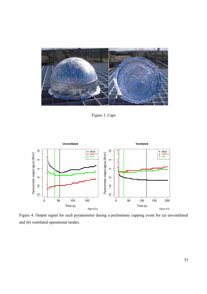
Figure 3. Caps

Figure 4. Output signal for each pyranometer during a preliminary capping event for (a) unventilated

and (b) ventilated operational modes.

33

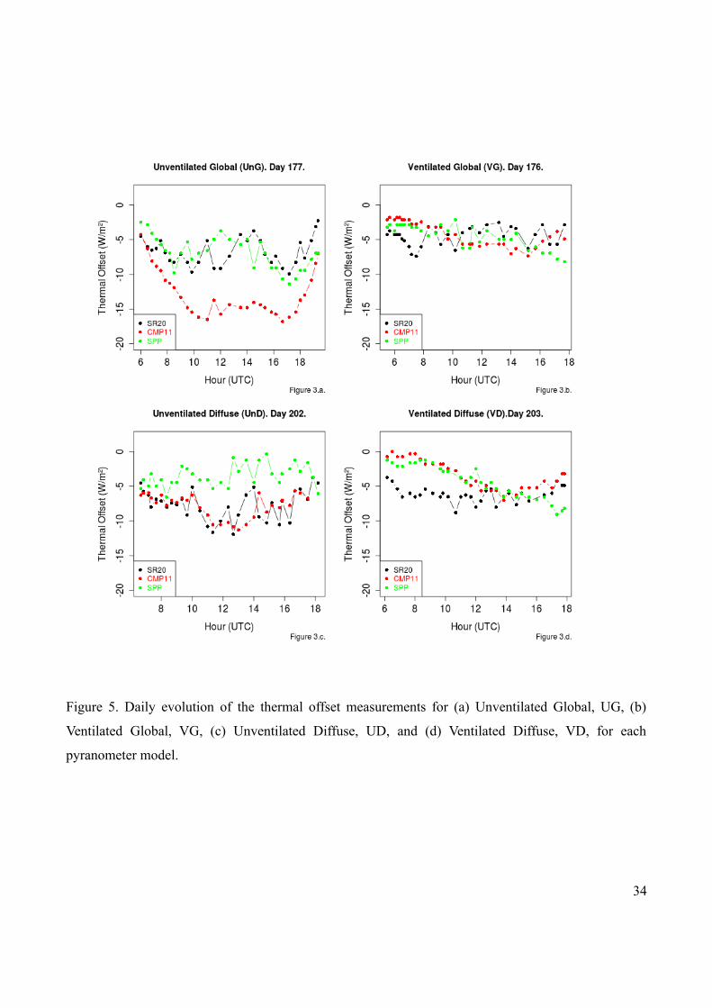
Figure 5. Daily evolution of the thermal offset measurements for (a) Unventilated Global, UG, (b)

Ventilated Global, VG, (c) Unventilated Diffuse, UD, and (d) Ventilated Diffuse, VD, for each

pyranometer model.

34

Figure 6. Dependence on the environmental conditions when the pyranometers are measuring global irradiance with ventilation (red points)

and without ventilation (black points)

35

Figure 7. Dependence on the environmental conditions when the pyranometers are measuring diffuse irradiance with ventilation (red points)

and without ventilation (black points)

36

Figure 8. Unventilated nighttime thermal offset versus Net IR irradiance. Solid grey line correspond to

the fitting forzed thtough (0,0) while dashed black line represent the no-forced fitting.

Figure 9. Absolute difference between daytime experimental thermal offset and those values estimated

by the application of the Dutton et al.’s methodology (fitting forzed through (0,0)).

37

3.5. ARTICULO 4 125


El artıculo .Effect of mechanical ventilation on the thermal offset of pyranome-

ters”, esta finalizando el proceso de revision en la revista Journal of Atmospheric

and Oceanic Technology, siendo previsible su publicacion definitiva durante el ano

2017, teniendo la revista un factor de impacto de 2.159 y estando incluida en el


Ocean”.



etapas desarrolladas para la obtencion del artıculo, como el diseno y realizacion de las

medidas, el analisis de resultados y comparativa, la extraccion de conclusiones y la

elaboracion del manuscrito. Merece la pena destacar el gran esfuerzo invertido por la

doctoranda para llevar a cabo la exigente toma de medidas disenada para el trabajo.




Por otra parte, D. Antonio Serrano Perez y Dna. Marıa Luisa Cancillo

Fernandez, coautores de este artıculo, afirman mediante este escrito que han

colaborado en este artıculo pero que este forma parte ıntegra de la Tesis Doctoral

de Dna. Guadalupe Sanchez Hernandez y que no va a ser utilizado por ellos como

parte de sus respectivas tesis doctorales


Capıtulo 4

Correccion del error introducido

por el anillo de sombra

4.1. Introduccion

Como ya se comento en el Capıtulo 1, debido a su diseno el anillo de sombra

bloquea, ademas de la componente directa, la irradiancia difusa interceptada por el

anillo. Esto conlleva una subestimacion de la medida de irradiancia difusa por lo

que estas medidas han de ser corregida.

La correccion del error asociado al uso del anillo de sombra depende de

numerosos factores y varıa con cada medida. Por un lado, las dimensiones del anillo

y su localizacion geografica determinan el angulo solido subtendido por el mismo

[Drummond, 1956]. Por otro lado, las condiciones atmosfericas y la posicion solar

determinan la distribucion direccional del campo de irradiancia difusa [Steven,

1984; LeBaron et al., 1990; Batlles et al., 1995]. Todos estos factores hacen que la

subestimacion de los valores de irradiancia total difusa medidos con este dispositivo

pueda llegar a suponer entre el 9 % y el 38 % de la medida [Kudish e Ianetz, 1993].

Este error supera notablemente el valor de incertidumbre del 2 % exigido por la

OMM para las medidas de irradiancia difusa de calidad [Ohmura et al., 1998;

McArthur, 2005; WMO, 2014].

Dada la importancia del error producido por el anillo de sombra varios autores

han propuesto diferentes modelos para su correccion. De este modo, los valores reales

de irradiancia difusa (Id,r) pueden obtenerse mediante la aplicacion de un factor de

correccion (C) a las medidas tomadas por un piranometro instalado en un anillo de

sombra (Id,u) tal como refleja la siguiente expresion:

127

128 CAPITULO 4. CORRECCION DEL ERROR INTRODUCIDO POR EL ANILLO DE SOMBRA

Id,r = C · Id,u (4.1)

Como una primera aproximacion al problema, Drummond [1956] propuso la

aplicacion de un factor de correccion, CD, basado exclusivamente en calculos de

geometrıa solar y bajo la hipotesis de una distribucion isotropa del campo de

radiacion difusa. Este modelo teorico proporciona una estimacion muy precisa del

angulo solido subtendido por el anillo y puede ser aplicado en cualquier localizacion

e intervalo espectral.

Sin embargo, la presencia y distribucion espacial de nubes y aerosoles ası como

la variacion de la posicion solar hacen que la hipotesis de isotropıa para el campo

de radiacion difusa raramente se cumpla. El propio Drummond [1956] estimo que

las medidas de irradiancia difusa una vez corregidas con su modelos requerıan

una correccion adicional del 7 % en caso de cielos despejados y del 3 % en casos

cubiertos debido a la anisotropıa de la radiacion. Estudios posteriores en diferentes

localizaciones estimaron el valor de esta correccion adicional entre un 14 % y 30 %

[Stanhill, 1985; Kudish e Ianetz, 1993].

Con el fin de corregir el efecto de la anisotropıa, algunos autores propusieron

nuevos modelos para la correccion del error debido al anillo de sombra. Estos

nuevos modelos proponen expresiones para el factor de correccion que incorporan

informacion sobre la distribucion del campo de radiacion difusa. Esta informacion

se introduce de dos formas diferentes: 1) utilizando modelos teoricos para la

distribucion del campo de radiacion y 2) mediante parametros empıricos calculados

a partir de datos de radiacion. Entre ellos destacan el modelo teorico propuesto

por Muneer y Zhang [2002] y los modelos empıricos propuestos por Steven [1984],

LeBaron et al. [1990] y Batlles et al. [1995].

La revision de los trabajos anteriormente mencionados junto con otros estudios

posteriores sobre la correccion del error introducido por el anillo de sombra puso

de manifiesto la existencia de importantes aspectos aun sin resolver entre los que

destacan:

Las escasez de estudios comparativos de los distintos modelos propuestos bajo

las mismas condiciones meteorologicas. Aunque estos modelos han sido apli-

cados en numerosas ocasiones por separado, son muy pocos los estudios en

los que han sido comparados [Batlles et al., 1995; Lopez et al., 2004a, 2004b;

Kudish y Evseev, 2008].

4.1. INTRODUCCION 129

El uso de valores de irradiancia difusa estimados como diferencia de irradiancia

global y directa como valores de referencia. Los valores de irradiancia difusa

ası estimados presentan una gran incertidumbre debido, principalmente, a la

limitaciones en la respuesta angular (error coseno) del piranometro que mide

los valores de irradiancia global [Michalsky et al., 1999].

La aplicacion de los coeficientes empıricos del modelo original. A pesar del

importante error que podrıa suponer no adaptar los modelos empıricos a las

caracterısticas locales propias de cada ubicacion son muy escasos los estudios

que han llamado la atencion sobre este aspecto [Dehne, 1984].

La ausencia de modelos para la correccion del error introducido por el ani-

llo de sombra en medidas de irradiancia difusa ultravioleta. Entre la amplia

bibliografıa analizada solo el trabajo realizado por Utrillas et al. [2007] trata

este aspecto.

Todos estos aspectos han sido analizados con detalle en los dos artıculos que

componen este capıtulo. Ambos trabajos suponen una importante contribucion a

la caracterizacion del error introducido por el anillo de sombra en las medidas de

irradiancia difusa total y UV, respectivamente.


4.2. Artıculo 5


Tıtulo: Comparison of shadow-ring correction models for diffuse solar irradiance


Antonio Serranoa

Mª Luisa Cancilloa

Jose Agustın Garcıaa


Revista: Journal of Geophysical Research-Atmosphere

Volumen: 117 Ano de publicacion: 2012

doi: 10.1029/2011JD017346

Este artıculo fue ademas seleccionado como “Spotlight Research”. Se trata de una

mencion especial que reciben, de entre todos los artıculos publicados en revistas de la

American Geophysical Union, aquellos que destacan por la calidad de su aportacion

cientıfica. Este reconocimiento dio lugar a una nota sobre nuestro artıculo, titulada

“New corrections for skylight estimates”, publicada en la revista Eos, volumen 93,

numero 31, pagina 308, el 31 de julio de 2012.


Este estudio tiene como objetivo seleccionar el modelo mas adecuado para la

correccion del error introducido por el anillo de sombra en las medidas de irradiancia

difusa total. Con este fin se ha seleccionado un conjunto de modelos representativo

de las distintas formas funcionales y variables propuestas en la bibliografıa. Los

modelos finalmente seleccionados han sido los propuestos por Drummond [1956],

Steven [1984], LeBaron et al. [1990], Batlles et al. [1995] y Muneer y Zhang [2002].

Para este estudio se ha utilizado un ano completo de datos horarios, lo que

garantiza trabajar con una gran variedad de situaciones meteorologicas. A diferencia

de los estudios anteriores en los que los valores de irradiancia difusa de referencia

eran estimados como diferencia de irradiancia global y directa, en este trabajo, los

valores de irradiancia difusa de referencia han sido medidos con un piranometro

instalado en un seguidor solar.

El primer paso, y uno de los puntos a destacar en este estudio, ha sido la

reproduccion de las metodologıas propuestas por Steven [1984], LeBaron et al.

4.2. ARTICULO 5 131

[1990] y Batlles et al. [1995] con medidas de nuestra estacion. Con ello se han

obtenido los correspondientes coeficientes empıricos para las expresiones propuestas

por Steven [1984] y Batlles et al. [1995] y los factores de correccion para cada

una de las 256 categorıas establecida por LeBaron et al. [1990]. Aunque la parti-

cularizacion de estos modelos a las medidas locales pueda parecer algo trivial, no

es una practica habitual en estudios similares y podrıa derivar en errores impor-

tantes. Una vez los modelos empıricos fueron particularizados se han comparado

con los modelos teoricos propuestos por Drummond [1956] y Muneer y Zhang [2002].

El analisis desarrollado en este artıculo revela que el factor de correccion

que debe aplicarse a las medidas de irradiancia total difusa medidas con anillo

de sombra (4.1) en nuestra estacion toma valores comprendidos entre 0.88 y

1.32. La subestimacion anual promedio en las medida de irradiancia difusa fue

estimada en torno a un 10.8 % pudiendo llegar a suponer hasta un 20 % en situa-

ciones de cielos despejados. Estos valores son similares a los obtenidos previamente

por otros autores [Kudish e Ianetz; 1993; Lopez et al., 2004b; Kudish y Evseev, 2008].

Como era de esperar, la adaptacion a las condiciones locales de los modelos

empıricos propuestos por Steven [1984], LeBaron et al. [1990] y Batlles et al. [1995],

supone una mejora tanto en su tendencia central como en su dispersion. Ademas,

dicha adaptacion elimina posibles dependencias de los residuos respecto a factores

como la posicion solar o el ındice de claridad, las cuales sı se observan en estudios en

los que los modelos no son adaptados [Lopez et al., 2004a; Kidish y Evseev, 2008].

Tambien debe mencionarse que los modelos teoricos propuestos por Drummond

[1956] y Muneer y Zhang [2002] muestran un comportamiento similar al de los

modelos empıricos sin adaptar. Por tanto, en caso de no ser posible la adaptacion

de los modelos empıricos, los modelos teoricos son igualmente validos.

La comparacion de los modelos teoricos propuestos por Durmmond [1956] y

Muneer y Zhang [2002] junto con los modelos empıricos adaptados de Steven [1984],

LeBaron et al. [1990] y Batlles et al. [1995] revela un mejor comportamiento de

estos ultimos. El valor medio de las diferencias relativas de 10.8 % en las medidas

sin corregir se reduce a 0.6 % al aplicar los modelos empıricos adaptados. Con la

aplicacion de estos modelos de correccion las diferencias relativas de las medidas

se encuentran dentro del error del 2 % requerido por la OMM en las medidas de

calidad.


4.2.3. Copia original de artıculo

Comparison of shadow-ring correction modelsfor diffuse solar irradiance

G. Sánchez,1 A. Serrano,1 M. L. Cancillo,1 and J. A. García1

Received 20 December 2011; revised 23 March 2012; accepted 28 March 2012; published 9 May 2012.

[1] Reliable and accurate measurements of diffuse solar irradiance are needed in orderto partition global irradiance into its direct and diffuse components. Diffuse irradiance iscommonly measured using sun tracking systems or shadow rings. Data obtained using ashadow ring must be corrected for the portion of diffuse irradiance blocked by the ring.In this paper we have examined and evaluated six of the most widely used correctionmodels. Approaches that account for radiation anisotropy perform notably better than thoseusing only geometric corrections. Our results also argue for the need to adjust empiricalmodels to local conditions. Empirical approaches developed by LeBaron et al. (1990) andby Batlles et al. (1995) perform best when compared with the more theoretical models.

Citation: Sánchez, G., A. Serrano, M. L. Cancillo, and J. A. García (2012), Comparison of shadow-ring correction models fordiffuse solar irradiance, J. Geophys. Res., 117, D09206, doi:10.1029/2011JD017346.

1. Introduction

[2] Many solar radiation studies rely on a good knowledgeof not only global radiation but on its direct and diffuse com-ponents as well. The accurate assessment of global and diffusesolar radiation is essential for estimating the radiation inter-cepted by horizontal and tilted surfaces such as hills, buildings,vegetation, and animals. In addition to meteorological studies,solar radiation data is used in many applications such as inarchitecture, engineering, agriculture and ecology.[3] The amount of diffuse radiation reaching the earth’s

surface and its proportion to global radiation is mainlydetermined by the solar zenith angle, the composition of theatmosphere, and surface albedo. Most of the atmosphericconstituents are relatively constant in time and space withthe exception of aerosols and clouds. Their interaction withsolar radiation is complex and any change of these con-stituents in a changing climate will affect the amount ofdirect and diffuse radiation reaching the earth’s surface andconsequently, the surface energy balance. Therefore, veryaccurate measurements of global, direct, and diffuse solarradiation at the earth’s surface are required to suitably detectand quantify the effect of climate change on the earth’sradiation balance [Hansen et al., 2005; Wild et al., 2005].[4] Information on the relative amount of direct and dif-

fuse solar irradiance that is available is also required in therapidly developing field of renewable energy. There arepresently considerable efforts being devoted to improvingthe efficiency of solar collectors, relying mainly on better

collecting systems. An accurate knowledge of the direct anddiffuse components of the radiation field is absolutelyessential to achieve this goal.[5] There are different instruments and methodologies

aimed to measure solar diffuse radiation. The most precisemethod consists of shading the pyranometer with a smalldisc or ball synchronized with the sun’s apparent motion.However, the technique is costly, requiring much mainte-nance and is unstable under strong winds. A more practicaland widely used approach is to measure diffuse radiationusing a shadow-ring/band. This is a robust mechanismconsisting in a ring/band parallel to the sun path that blocksthe direct irradiance and prevents it from reaching the sen-sor. It is an easy-to-operate stationary device that onlyrequires manual adjustment of the sliding bar every few daysto account for changing solar declination. The shadow bandsystem is the most common method for measuring diffuseradiation at meteorological stations worldwide. Thus, longtime series of diffuse radiation measurements using shadingrings exist since the first half of the last century. Somestudies have shown that measurements with shadow ringsare comparable to those given by more sophisticated track-ing devices under totally cloudy skies whereas in clear skyconditions some differences appear [Ineichen et al., 1984].[6] The shadow ring screens not only the sun’s disc but

also a substantial portion of the sky and, therefore, its mea-surements must be corrected for the diffuse radiation inter-cepted by the ring. This error can, for example, result in amonthly average error of up to 24% [Drummond, 1956],significantly affecting any subsequent calculation of otherradiometric variables. Thus, a 5% error in the measurementof the horizontal diffuse irradiance will propagate to morethan 20% in the calculated direct normal irradiance at zenithangles greater than 75� [LeBaron et al., 1990]. The neededcorrection factor has been estimated to be between 8.9% and37.7% [Kudish and Ianetz, 1993], depending on the latitude,the weather conditions and the type of the shadow ring

1Department of Physics, University of Extremadura, Badajoz, Spain.

Corresponding author: G. Sánchez, Department of Physics, Universityof Extremadura, Avda. de Elvas s/n, E-06006 Badajoz, Spain.([email protected])

Copyright 2012 by the American Geophysical Union.0148-0227/12/2011JD017346

JOURNAL OF GEOPHYSICAL RESEARCH, VOL. 117, D09206, doi:10.1029/2011JD017346, 2012

D09206 1 of 8

[Steven, 1984]. This uncertainty limits the accuracy of dif-fuse radiation measurements and makes it difficult to com-pare measurements performed at different locations ordifferent seasons [Drummond, 1956; Steven, 1984]. Toemphasize the importance of this correction, it must be notedthat it is higher than the variation in solar radiation observedbetween 1961 and 1990, estimated to be around the 4–6%[Liepert, 2002], and higher than the accuracy of �3%required by the World Meteorological Organization for aparticular measurement to be classified as high quality[World Meteorological Organization (WMO), 2008].[7] As a first approach to the problem, Drummond [1956]

proposed a first correction factor as a function of the solidangle subtended by the shadow ring and its altitude abovethe pyranometer horizon. This model is exclusively based onsolar geometry calculations and assumes an isotropic skyradiation distribution. It provides a fairly good estimation ofdiffuse irradiance occluded by the ring and may be appliedanywhere on earth. However, the assumption of isotropy isnot generally fulfilled since sky radiance directional distri-bution notably depends on sun elevation, atmospheric turbid-ity, cloudiness and usually changes with weather conditionsduring the day. Thus,Drummond [1956] estimated differencesof about 7% for cloudless skies and 3% for overcast conditionsbetween its corrected diffuse irradiance values and the refer-ence values due to the anisotropy. Other subsequent studiesquantified the additional correction for anisotropic conditionsto be between 14% and 30% above the isotropic correction[Stanhill, 1985]. Several models have been developed in orderto correct for the anisotropy effect. A straightforward modifi-cation to the Drummond’s model was proposed by Steven[1984], who assumed a sky radiance distribution as the sumof a uniform background and a circumsolar component. On theother hand, LeBaron et al. [1990] developed a model whichclassified the different sky conditions into 256 categories as afunction of three parameters describing the anisotropic contri-bution and the fraction of the sky hemisphere occluded by theshadow ring as estimated by Drummond [1956]. Using thesame parameters than Le Baron et al., Batlles et al. [1995]proposed two correction factors as multivariate-lineal func-tions of these parameters. More recently, Muneer and Zhang[2002] have developed a new model based on the anisotropicsky-diffuse distribution theory proposed byMoon and Spencer[1942].[8] Comparative studies are required in order to assess the

performance and limitations of these models and their suit-ability at different locations in the world. However, to ourknowledge, there are few comparative studies [López et al.,2004a, 2004b; Kudish and Evseev, 2008], and even fewerfor regions with similar climatic characteristics as our studysite in southwestern Europe. Additionally, most recent stud-ies applied the models using the original values of localparameters as they were proposed by their respective authors,although Dehne [1984] noted the need to use coefficientsapplicable to the local study areas. Failure to do so may createlarge errors since some of these models have been developedempirically and their correction factors depend on the geo-graphical and climatic characteristics of each location.[9] Therefore, the main objectives of this paper are to assess

the performance of the models proposed by Drummond[1956], Steven [1984], LeBaron et al. [1990], Batlles et al.[1995] and Muneer and Zhang [2002] in estimating diffuse

irradiance measured with a pyranometer and a shadow-ring atBadajoz (southwestern Spain) and to examine how the coef-ficients of these empirical models need to be adapted to newsites. These models will be called DR (Drummond), ST(Steven), LB (LeBaron et al.), BA or BB (Models A and B byBatlles et al.), and MZ (Muneer and Zhang) hereafter. All thementioned models have been extensively used in differentclimatic regions throughout the world [López et al., 2004a,2004b; Kudish and Evseev, 2008] and are well considered bythe scientific community. In this study we evaluate the suit-ability of the empirical models ST, LB, BA and BB to ourstudy site and examine the sensitivity of the various coeffi-cients to the estimate of diffuse radiation. Finally, theseadjusted models are compared with the theoretical modelsDR and MZ.

2. Data

[10] Data used in this study have been acquired at theradiometric station installed in Badajoz, southwestern ofSpain (38.9� N; 7.01� W; 199 m a.s.l). The site has an openhorizon, free of obstacles and is operated by the PhysicsDepartment of the University of Extremadura, guaranteeingcareful maintenance. The local climate is characterized byhigh noon solar elevation, mainly in summer, and by a highnumber of sunshine hours per year, with our site having oneof the highest instantaneous and annual irradiance values inEurope.[11] The data set consists of one-minute measurements of

horizontal global irradiance and two simultaneous measure-ments of diffuse irradiance using two different methods. Thediffuse solar irradiance was measured using a Kipp & ZonenCMP11 pyranometer which was shaded using a Kipp & ZonenCM121 shadow-ring with 620 mm diameter and 55 mmwidth.Simultaneous measurements of diffuse solar irradiance weretaken by another CMP11 pyranometer mounted on a solartracker (Kipp& Zonen Solys 2). The solar tracker has a ball thatprevents the direct solar irradiance to reach the sensor. The ballonly shadows the pyranometer sensor and does not obstruct anyother sky portion. The correction factor for these measurementsis negligible [Ineichen et al., 1984] and therefore they havebeen used as a reference. A third Kipp & Zonen CMP11 pyr-anometer was used to measure global irradiance. The studyperiod encompassed an entire year, from 7 August 2010 to8 August 2011, therefore ensuring that a variety of seasonalprocesses and meteorological conditions were sampled.[12] To guarantee the quality and comparability of mea-

surements, both pyranometers were previously inter-comparedand calibrated in a field campaign which took place in Sep-tember 2009 at the Atmospheric Sounding Station of theNational Institute for Aerospace Techniques (ESAt/ INTA)located at “El Arenosillo,”Huelva, Spain (37.10� N, 7.06� W).The pyranometers were calibrated by intercomparison with areference pyranometer (Kipp & Zonen CM11 pyranometer,#027771) which had been previously calibrated at the WorldRadiation Centre (WRC) in Davos, Switzerland. First, signalswere corrected for thermal offsets estimated as the averages ofvalues recorded for solar zenith angles higher than 100�. Then,ratios of our pyranometer signal to the signal from the refer-ence pyranometer were estimated for a range of conditions.They proved to be largely constant so that calibration factors

SÁNCHEZ ET AL.: CORRECTION MODELS FOR DIFFUSE IRRADIANCE D09206D09206

2 of 8

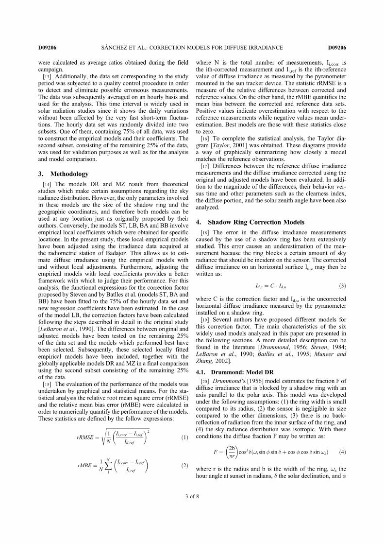
were calculated as average ratios obtained during the fieldcampaign.[13] Additionally, the data set corresponding to the study

period was subjected to a quality control procedure in orderto detect and eliminate possible erroneous measurements.The data was subsequently averaged on an hourly basis andused for the analysis. This time interval is widely used insolar radiation studies since it shows the daily variationswithout been affected by the very fast short-term fluctua-tions. The hourly data set was randomly divided into twosubsets. One of them, containing 75% of all data, was usedto construct the empirical models and their coefficients. Thesecond subset, consisting of the remaining 25% of the data,was used for validation purposes as well as for the analysisand model comparison.

3. Methodology

[14] The models DR and MZ result from theoreticalstudies which make certain assumptions regarding the skyradiance distribution. However, the only parameters involvedin these models are the size of the shadow ring and thegeographic coordinates, and therefore both models can beused at any location just as originally proposed by theirauthors. Conversely, the models ST, LB, BA and BB involveempirical local coefficients which were obtained for specificlocations. In the present study, these local empirical modelshave been adjusted using the irradiance data acquired atthe radiometric station of Badajoz. This allows us to esti-mate diffuse irradiance using the empirical models withand without local adjustments. Furthermore, adjusting theempirical models with local coefficients provides a betterframework with which to judge their performance. For thisanalysis, the functional expressions for the correction factorproposed by Steven and by Batlles et al. (models ST, BA andBB) have been fitted to the 75% of the hourly data set andnew regression coefficients have been estimated. In the caseof the model LB, the correction factors have been calculatedfollowing the steps described in detail in the original study[LeBaron et al., 1990]. The differences between original andadjusted models have been tested on the remaining 25%of the data set and the models which performed best havebeen selected. Subsequently, these selected locally fittedempirical models have been included, together with theglobally applicable models DR and MZ in a final comparisonusing the second subset consisting of the remaining 25%of the data.[15] The evaluation of the performance of the models was

undertaken by graphical and statistical means. For the sta-tistical analysis the relative root mean square error (rRMSE)and the relative mean bias error (rMBE) were calculated inorder to numerically quantify the performance of the models.These statistics are defined by the follow expressions:

rRMSE ¼ffiffiffiffiffiffiffiffiffiffiffiffiffiffiffiffiffiffiffiffiffiffiffiffiffiffiffiffiffiffiffiffiffiffiffiffiffi1

N

Ii;corr � Ii;refId;ref

� �2s

ð1Þ

rMBE ¼ 1

N

XN1

Ii;corr � Ii;refIi;ref

� �ð2Þ

where N is the total number of measurements, Ii,corr isthe ith-corrected measurement and Ii,ref is the ith-referencevalue of diffuse irradiance as measured by the pyranometermounted in the sun tracker device. The statistic rRMSE is ameasure of the relative differences between corrected andreference values. On the other hand, the rMBE quantifies themean bias between the corrected and reference data sets.Positive values indicate overestimation with respect to thereference measurements while negative values mean under-estimation. Best models are those with these statistics closeto zero.[16] To complete the statistical analysis, the Taylor dia-

gram [Taylor, 2001] was obtained. These diagrams providea way of graphically summarizing how closely a modelmatches the reference observations.[17] Differences between the reference diffuse irradiance

measurements and the diffuse irradiance corrected using theoriginal and adjusted models have been evaluated. In addi-tion to the magnitude of the differences, their behavior ver-sus time and other parameters such as the clearness index,the diffuse portion, and the solar zenith angle have been alsoanalyzed.

4. Shadow Ring Correction Models

[18] The error in the diffuse irradiance measurementscaused by the use of a shadow ring has been extensivelystudied. This error causes an underestimation of the mea-surement because the ring blocks a certain amount of skyradiance that should be incident on the sensor. The correcteddiffuse irradiance on an horizontal surface Id,c may then bewritten as:

Id;c ¼ C � Id;u ð3Þ

where C is the correction factor and Id,u is the uncorrectedhorizontal diffuse irradiance measured by the pyranometerinstalled on a shadow ring.[19] Several authors have proposed different models for

this correction factor. The main characteristics of the sixwidely used models analyzed in this paper are presented inthe following sections. A more detailed description can befound in the literature [Drummond, 1956; Steven, 1984;LeBaron et al., 1990; Batlles et al., 1995; Muneer andZhang, 2002].

4.1. Drummond: Model DR

[20] Drummond’s [1956] model estimates the fraction F ofdiffuse irradiance that is blocked by a shadow ring with anaxis parallel to the polar axis. This model was developedunder the following assumptions: (1) the ring width is smallcompared to its radius, (2) the sensor is negligible in sizecompared to the other dimensions, (3) there is no back-reflection of radiation from the inner surface of the ring, and(4) the sky radiance distribution was isotropic. With theseconditions the diffuse fraction F may be written as:

F ¼ 2b

pr

� �cos3d wssin f sin d þ cos f cos d sin wsð Þ ð4Þ

where r is the radius and b is the width of the ring, ws thehour angle at sunset in radians, d the solar declination, and f


3 of 8

the latitude of the location. The correction factor proposed inthis model is:

CD ¼ 1

1� Fð5Þ

4.2. Steven: Model ST

[21] Based on previous studies, Steven [1984] proposed anew model for the correction factor to use under clear con-ditions. This model introduces an additional anisotropyfactor independent of the geometrical correction. The mainhypothesis is that the sky radiance distribution is the sum ofa uniform background and a circumsolar component. Thecorrection factor proposed is:

CS ¼ Id;refId;u

¼ 1

1� FQð6Þ

where F is the fraction of diffuse irradiance occluded by thering given by the equation (4) and Q is the anisotropy cor-rection factor calculated using the follow expressions:

Q ¼ 1� C′x þ C′

fð7Þ

f ¼ wssin f sin d þ cos f cos d sin ws ð8Þ

where C′ expresses the relative strength of the circumsolarcomponent and x is the angular width of the circumsolarregion. These coefficients can be obtained by means of aregression analysis of Q values (calculated from equation (6)as a function of the reference diffuse irradiance, uncorrecteddiffuse irradiance and the portion of diffuse irradianceblocked by the ring) versus 1/f values.

4.3. LeBaron et al.: Model LB

[22] The model proposed by LeBaron et al. [1990]describes anisotropic sky conditions by means of threeparameters. One of these parameters, ɛ, describes the cloudconditions and is defined as:

ɛ ¼ Id;u þ InbId;u

ð9Þ

where Id,u is the uncorrected diffuse irradiance and Inb is theuncorrected direct normal irradiance which can be calculatedfrom the global and uncorrected diffuse irradiance.[23] The second parameter D is a brightness index which

is a function of the cloud thickness or aerosol loading [Perezet al., 1990]. It is defined as:

D ¼ Id;u � mI0

ð10Þ

where m is the relative optical air mass and I0 is the irradi-ance at the top of the atmosphere.[24] The third parameter is the solar zenith angle q. These

three parameters, together with the isotropy correction CD

proposed by Drummond [1956], are used to classify thedifferent sky conditions into 256 categories. These catego-ries are the results of the combination of the four possiblevalues that each parameter can take. The range of eachparameter was divided in four subintervals. Subsequently,

the reference and uncorrected diffuse irradiance measure-ments were classified according to the categories defined bythe combination of the parameters and, finally, the correctionfactor for each category was obtained as the average of theratio between the reference diffuse irradiance measurementsand the uncorrected diffuse irradiance measurements. Moredetails can be found in LeBaron et al. [1990].

4.4. Batlles et al.: Models BA and BB

[25] Based on the same parameters utilized in model LB,Batlles et al. [1995] built two new models to correct thediffuse irradiance measured with shadow rings. Both modelsuse a multiple linear regression of these parameters to obtainthe correction factors. In this paper these models will becalled BA and BB.4.4.1. Model BA[26] This first model proposes an unique expression of the

correction factor for all sky conditions:

CBA ¼ aCD þ blogDþ clogɛþ de �1= cosqð Þ ð11Þ

where CD, ɛ and D were defined in equations (5), (9) and(10) respectively and a, b, c, and d areempirical parameters.4.4.2. Model BB[27] After the geometric correction, the parameter ɛ is the

second most significant parameter in the correction factoranalysis. Based on this fact, Batlles et al. [1995] proposeddifferent multiple linear regressions with appropriate func-tions of CD, D, and q for different ranges of ɛ. The resultantmodel is described by the following set of equations:

CBB ¼ a1CD þ b1logDþ d1e ð�1=cosqÞ ɛ ≤ 3:5 ð12aÞ

CBB ¼ a2CD þ b2logDþ d2e ð�1=cosqÞ 3:5 < ɛ ≤ 8 ð12bÞ

CBB ¼ a3CD þ b3logD 8 < ɛ ≤ 11 ð12cÞ

CBB ¼ a4CD þ b4logD 11 < ɛ ð12dÞ

where a1, b1, d1, a2, b2, d2, a3, b3, a4, and b4 are obtained byregression analysis. More details can be found in Batlleset al. [1995].

4.5. Muneer and Zhang: Model MZ

[28] Muneer and Zhang [2002] developed a methodologysimilar to the one applied in model DR but using a newirradiance distribution. This irradiance distribution wasbased on the model proposed by Moon and Spencer [1942]and revised by Muneer [1990]. According to this model,the sky radiance distribution is two dimensional and functionof any given sky patch geometry (sky patch altitude andazimuth) and the position of the sun. This new irradiancedistribution can be used to estimate the total diffuse irradi-ance that is blocked by the shadow ring as follows:

D ¼ b

rLzcos

3dI1 þ b1I21þ b1

� �ð13Þ


4 of 8

where Lz is the zenith radiance, b is the width of the shadowring, r is its radio, and d is the solar declination. ParametersI1 and I2 are defined by the follow expressions:

I1 ¼ wssin f sin d þ cos f cos d sin ws ð14Þ

I2 ¼ wssin2f sin2d þ 2 sin ws sin f cos f sin d cos d

þ cos2f cos dws

2þ sin 2ws

4

� �ð15Þ

Using this same irradiance distribution, the total diffuseirradiance Id is calculated by means of numerical integrationwhich gives the following expression:

Id ¼ pLz6

3þ 2b11þ b1

þ 3þ 2b21þ b2

� �ð16Þ

where b1 and b2 are radiance distribution indices for the skyquadrants containing the sun and the opposed quadrant,respectively, which are estimated as follows:

If kt > 0:2 b1 ¼ 3:6� 10:46kt�0:4þ 6:974kt

ð17aÞ

b2 ¼ 1:565� 0:990kt0:957þ 0:660kt

ð17bÞ

If kt ≤ 0:2 b1 ¼ b2 ¼ 1:68 ð18Þ

Finally, the correction factor given by this model is:

CM ¼ 1

1� D

Id

ð19Þ

5. Results and Discussion

5.1. Fitting Local Models

[29] The empirical models ST, LB, BA and BB were fittedto local conditions and the resulting parameters comparedwith the original parameters listed by the authors in order toassess their general validity. The new correction factors ofthe models ST, BA and BB were obtained by means ofregression analyses using 75% of the data measured at ourradiometric station. Similarly, the model LB was adjusted tolocal conditions using the same 75% data set. Subsequently,the new adjusted models were compared with the originalmodels using the remaining 25% of the data.

[30] Diffuse irradiance corrections using the original andmodified methods are compared next. Differences in theestimation of diffuse irradiance between the original andthe adjusted model ST can be up to 4.7% and with a meanof 3.1%. The mean difference is 3.2% for the model LB,although individual values can exceed 16.0% and differ-ences are higher than 5% in 15.7% of the cases examined.Mean differences of 1.7% and 2.0% are obtained for modelsBA and BB with largest differences of up to 15% and 9.2%respectively being reached in high solar zenith angle con-ditions. The generally low values in the mean differencefound for models BA and BB could be explained by the factthat these models were originally developed for two Spanishsites in a geographical region similar to ours. However,dispersion is high when considering individual differences inall of the above three models. One possibility could be thaterrors are introduced by the parameters ɛ and D, related tocloud cover and brightening conditions, and which mightnot be totally applicable and valid for our region.[31] In the above paragraph we examined how the modi-

fied models differed from the originals. Here we assess theperformance of these modified models against a referencediffuse measurement which is considered a true value. TherRMSE and rMBE values with respect to the referencemeasurements were obtained for the original and for theadjusted models (Table 1). The aim of this analysis is tocheck the improvement achieved by the adjusted models. Itmay be observed that the biases shown by the originalmodels are largely eliminated in the adjusted models whichapproach zero. The rRMSE values improve by 0.67% for themodel ST (from 4.02% to 3.35%) and by 2.06% for themodel LB (from 4.67% to 2.61%). It may be concluded thatuse of empirical models with locally derived coefficientsconsiderably improves the diffuse correction process inshadow-ring measurements. This supremacy of adjustedmodels relies on their ability to be adapted to locally specificatmospheric and surface albedo conditions.[32] Kudish and Ianetz [1993] estimated the magnitude of

the shadow-ring correction factor to be between 8.9% and37.7%. In our study we obtained a mean difference of 10.8%between the uncorrected and the reference diffuse irradiancemeasurement. These differences are considerable and there-fore any improvement in the correction methodology isvaluable and justified. An overall assessment is performed inthe next section where the locally fitted version of theempirical models are compared with the globally valid the-oretical models DR and MZ.

5.2. Comparative Analysis of the Models

[33] Figures 1a–1g show the uncorrected and correcteddiffuse irradiances versus the reference diffuse irradiancesfor the six models. In general, the measurements exhibit abetter performance when corrections are applied. However,although the correction applied by the model DR notablyimproves the estimation of diffuse irradiance, it still under-estimates the reference values. Conversely, this underesti-mation is no longer evident in the correction models whichconsider anisotropy. However, all model/reference differ-ences feature much scatter when diffuse irradiance valuesare high. This is likely due to the large variety of possiblediffuse radiation values associated with cloudy conditions.

Table 1. The rRMSE and rMBE Values for the Original andAdjusted Models

Model Author

Original Models Adjusted Models

rRMSE (%) rMBE (%) rRMSE (%) rMBE (%)

ST Steven 4.02 1.19 3.35 �0.04LB LeBaron et al. 4.67 �1.20 2.61 0.01BA Batlles et al. 4.47 0.65 3.42 0.05BB Batlles et al. 4.39 0.78 3.20 0.01


5 of 8

Figure 1. (a) Uncorrected and (b–g) corrected diffuse irradiances versus the reference diffuse irradiancesfor the six models.


6 of 8

[34] Table 2 shows the statistics rRMSE and rMBE for theuncorrected measurements and the various correction mod-els versus the reference measurements. While the rRMSE foruncorrected measurements is about 7.48%, it decreases tovalues between 2.61% and 4.34% for the corrected mea-surements. According to this statistic, the model with thebest performance is model LB (2.61%) followed by themodel BB (3.20%). By contrast the models with the highestrRMSE values are the globally valid theoretical models DRand MZ. All models with the exception of DR estimatediffuse irradiance with a low rMBE. The model DR showsan underestimation in the rMBE of �1.4% as it does notconsider the anisotropy in the spatial distribution of theradiation field.[35] Results also indicate that the locally fitted empirical

models (ST, LB, BA and BB) perform better than theglobally valid theoretical models (DR and MZ). We alsonote the fairly good performance shown by the model STdespite being originally developed for cloudless conditions.This good general behavior may be related to the fact thatcloudless conditions are very frequent in our region. Thebest performance is achieved by the model LB followed bythe models Ba and BB. These three models feature theparameters ɛ and D that seem to describe the anisotropy

effect better than other model parameters such kt in themodel MZ, or the circumsolar region characteristics, C and x,in the model ST. The main difference between these twobest-performing models is that, while the model LB esti-mates the correction factor as a direct average of a certainsubset of the experimental data, models BA and BB proposespecific functional expressions which are fitted by regres-sion. On the negative side we note that the model LB needs aconsiderable amount of computation to obtain a calibrationfactor for each of the 256 categories.[36] In order to have a complete comparison of the per-

formance of the different models, the Taylor diagram wasplotted (Figure 2). This diagram provides a graphical sum-mary of different aspects of the performance of a model,such as the centered root-mean square error, the correlationand the magnitude of its differences with respect to the ref-erence values [Taylor, 2001]. Therefore, it is a suitable toolfor model comparison. Figure 2 shows the very good per-formance of the models LB, BB and BB, followed by themodels ST, DR and MZ, and ending with the uncorrectedmeasurements.[37] An additional analysis was performed in order to

better understand the reasons for the differences between thevarious models and the reference measurement. These dif-ferences were analyzed as a function of the solar zenithangle, the clearness index, and the ratio of diffuse-to-globalsolar irradiance kd. No significant dependence was foundwith the solar altitude or with the clearness index, but certaindifferences between models appeared in the case of kd(Figure 3). While the models LB, BB and BA suitablyaccount for the dependence with kd, the models DR, ST andMZ correct for this dependence only partially.

6. Conclusions

[38] In this study, the six most widely used models forcorrecting horizontal diffuse irradiance measured with ashadow ring have been analyzed and compared. First, the

Table 2. Values of rRMSE and rMBE for Uncorrected Measure-ment and for Corrected Measurements Using the CorrectionModels Shown Here

Model rRMSE (%) rMBE (%)

Uncorrected 7.48 �4.29DR 4.35 �1.43ST 3.35 �0.04LB 2.61 0.05BA 3.42 0.01BB 3.20 0.01MZ 4.34 0.06

Figure 2. Taylor diagram.Figure 3. Dependence of relative differences on the ratio ofdiffuse-to-global solar irradiance kd.


7 of 8

parameters of the empirical models ST, LB, BA and BB wereadjusted for local conditions as determined by our radiometricmeasurements in Badajoz, southwestern Europe. The locallyfitted versions of the original empirical models significantlyimproved the estimation as determined by the central tendency(quantified by rMBE) and the dispersion (quantified byrRMSE).We conclude that adjusting the empirical coefficientsfor local atmospheric and surface albedo conditions is war-ranted and recommend this procedure in other environmentsthat may differ from ours or from the environment associatedwith the original model development.[39] These locally fitted versions of the empirical models

were subsequently compared with the globally valid theo-retical models DR and MZ. Results show the remarkableimprovement achieved by the models which account forradiation anisotropy as contrasted with the model DR whichconsiders only a geometrical correction factor. The locallyfitted empirical models perform notably better than theglobally valid theoretical models. In particular, the modelsLB, BB and BA performed best, exhibiting the lowest valuesof both the rRMSE and rMBE statistics. All these results arealso confirmed by the global comparison performed bymeans of the Taylor diagram.[40] The analysis of residuals shows that they are inde-

pendent of both solar zenith angle and clearness index in allmodels. However, the models ST, DR and MZ proposed bySteven, Muneer and Zhang, and by Drummond show certaindependence of their residuals on kd, while the models LB,BB and BA show no dependence.[41] All these results argue for the use of locally adjusted

empirical models in order to correct for errors caused by theshadow ring when measuring solar diffuse irradiance. Themodel LB developed by LeBaron et al., and the models BB andBA by Battles et al. performed best for our specific location.[42] This study has made a positive contribution to the

methodology of measuring accurately the diffuse solar irradi-ance at the earth’s surface. Therefore, it provides usefulinformation for future studies which focus on estimating pre-cisely the earth’s radiation balance or studies which attempt toquantify the solar radiation resource for renewable energyapplications.

[43] Acknowledgments. This study was partially supported by theresearch projects CGL2008-05939-C03-02/CLI and CGL2011-29921-C02-01 granted by the “Ministerio de Ciencia e Innovación” from Spain.The authors thank Manuel Nunez for proofreading the text.

ReferencesBatlles, F. J., F. J. Olmo, and L. Alados-Arboleda (1995), On shadow bandcorrection methods for diffuse irradiance measurements, Sol. Energy, 54,105–114, doi:10.1016/0038-092X(94)00115-T.

Dehne, K. (1984), Diffuse solar radiation measured by the shade ringmethod improved by a correction formula, Rep. 15, World Meteorol.Org., Geneva, Switzerland.

Drummond, A. J. (1956), On the measurement of sky radiation, Arch.Meteorol. Geophys. Bioklimatol., Ser. B, 7, 413–436, doi:10.1007/BF02242969.

Hansen, J., et al. (2005), Earth’s energy imbalance: Confirmation and impli-cations, Science, 308, 1431–1435, doi:10.1126/science.1110252.

Ineichen, P., J. M. Gremaud, O. Guisan, and A. Mermoud (1984), Study ofthe corrective factor involved when measuring the diffuse solar radiationby use of the ring method, Sol. Energy, 32, 585–590, doi:10.1016/0038-092X(84)90133-6.

Kudish, A. I., and E. G. Evseev (2008), The assessment of four differentcorrection models applied to the diffuse radiation measured with a shadowring using global and normal beam radiation measurements for Beer Sheva,Israel, Sol. Energy, 82, 144–156, doi:10.1016/j.solener.2007.06.006.

Kudish, A. I., and A. Ianetz (1993), Analysis of diffuse radiation data forBeer Sheva: Measured (shadow ring) versus calculated (global-horizontalbeam) values, Sol. Energy, 51, 495–503, doi:10.1016/0038-092X(93)90134-A.

LeBaron, B. A., J. J. Michalsky, and R. Perez (1990), A simple procedurefor correcting shadow band data for all sky conditions, Sol. Energy, 44,249–256, doi:10.1016/0038-092X(90)90053-F.

Liepert, B. G. (2002), Observed reductions of surface solar radiation at sitesin the United States and worldwide from 1961 to 1990, Geophys. Res.Lett., 29(10), 1421, doi:10.1029/2002GL014910.

López, G., T. Muneer, and R. Claywell (2004a), Assessment of fourshadow band correction models using beam normal irradiance data fromthe United Kingdom and Israel, Energy Convers. Manage., 45, 1963–1979,doi:10.1016/j.enconman.2003.11.001.

López, G., T. Muneer, and R. Claywell (2004b), Comparative study of fourshadow band diffuse irradiance corrections algorithms for Almeria,Spain, J. Sol. Energy Eng., 126, 696–701, doi:10.1115/1.1666895.

Moon, P., and D. E. Spencer (1942), Illumination from a non-uniform sky,Trans. Illum. Eng. Soc., 37, 707–725.

Muneer, T. (1990), Solar radiation model for Europe, Build. Serv. Eng. Res.Technol., 11, 153–163.

Muneer, T., and X. Zhang (2002), A new method for correcting shadowband diffuse irradiance data, J. Sol. Energy Eng., 124, 34–43, doi:10.1115/1.1435647.

Perez, R., P. Ineichen, R. Seals, J. J. Michalsky, and R. Steward (1990),Modelling daylight availability and irradiance components from directand global irradiance, Sol. Energy, 44, 271–289, doi:10.1016/0038-092X(90)90055-H.

Stanhill, G. (1985), Observations of shade-ring corrections for diffuse skyradiation measurements at the dead sea, Q. J. R. Meteorol. Soc., 111(470),1125–1130, doi:10.1256/smsqj.47012.

Steven, M. D. (1984), The anisotropy of diffuse solar radiation determinedfrom shade-ring measurements, Q. J. R. Meteorol. Soc., 110, 261–270,doi:10.1002/qj.49711046317.

Taylor, K. E. (2001), Summarizing multiple aspects of model performancein a single diagram, J. Geophys. Res., 106, 7183–7192, doi:10.1029/2000JD900719.

Wild, M., H. Gilgen, A. Roesch, A. Ohmura, C. N. Long, E. G. Dutton,B. Forgan, A. Kallis, V. Russak, and A. Tsvetkov (2005), From dimmingto brightening: Decadal changes in solar radiation at Earth’s surface,Science, 308, 847–850, doi:10.1126/science.1103215.

World Meteorological Organization (WMO) (2008),Guide to MeteorologicalInstruments and Methods of Observation, 7th ed., Geneva, Switzerland.


8 of 8

4.2. ARTICULO 5 141


El artıculo Comparison of shadow-ring correction models for diffuse solar irra-

diance”, fue publicado en la revista Journal of Geophysical Research - Atmospheres

en mayo de 2012, teniendo la revista un factor de impacto en 2012 de 3.174 y

estando incluida en el primer cuartil (Q1, ranking 23 de 172 revistas) dentro de la

categorıa ”Geosciences, Multidisciplinary”.



etapas desarrolladas para la obtencion del artıculo, destacando su trabajo en la

toma de medidas, implementacion de los diferentes modelos y calculo, analisis de los

resultados y comparativa entre modelos, extraccion de conclusiones y elaboracion

del manuscrito.




Por otra parte, D. Antonio Serrano Perez, Dna. Marıa Luisa Cancillo Fernandez

y D. Jose Agustın Garcıa Garcıa, coautores de este artıculo, afirman mediante este

escrito que han colaborado en este artıculo pero que este forma parte ıntegra de la

Tesis Doctoral de Dna. Guadalupe Sanchez Hernandez y que no va a ser utilizado

por ellos como parte de sus respectivas tesis doctorales.

Dna. Mª Luisa Cancillo Fernandez D. Jose Agustın Garcıa Garcıa


4.3. Artıculo 6


Tıtulo: Shadow-band correction for diffuse ultraviolet radiation measurements


Antonio Serranoa

Mª Luisa Cancilloa


Revista: Journal of Geophysical Research-Atmosphere


doi: 10.1002/jgrd.50361


Este trabajo tiene como principal objetivo proponer modelos para la correc-

cion del error introducido por una banda de sombra en medidas de irradiancia

difusa UV. Para ello se han tomado como punto de partida algunos de los mode-

los propuestos para la correccion de este error en medidas de irradiancia difusa total.

Los modelos elegidos como puntos de partida para este estudio fueron los

propuestos por Drummond [1956], Steven [1984] y Batlles et al. [1995]. En este

trabajo no ha sido incluido el modelo propuesto por Muneer y Zhang [2002],

ya que dicho modelo parte del modelo de distribucion del campo de radiacion

difusa para el espectro solar total propuesto por Moon y Spencer [1942]. Por

tanto los coeficientes y expresiones que finalmente se obtuvieron para el modelo

de Muneer y Zhang son propias del espectro solar total y, en principio, podrıan

no ser adecuadas para el rango de longitudes de onda del UV. Basandonos en

los resultados del Artıculo 5, tambien decidimos no incluir el modelo propuesto

por LeBaron et al. [1990]. Se trata de un modelo complejo a nivel computacional

lo que dificulta su aplicacion. Al mismo tiempo, los modelos propuestos por

Batlles et al. [1995] incorporan sus mismos parametros para la descripcion de la

anisotropıa del campo de radiacion difusa y su adaptacion es mucho mas senci-

lla. Es por ello que ser prefirio la incorporacion de estos ultimos a este nuevo estudio.

La banda de sombra utilizada en este estudio fue cedida por el centro territorial

de AEMet en Extremadura y su uso habitual hasta entonces habıa sido la medida

de irradiancia difusa total. Es por ello que esta banda tuvo que ser adaptada para la

medida de irradiancia difusa UV tendiendo en cuenta la diferencia en altura de los

4.3. ARTICULO 6 143

piranometros y los radiometros de UV. Finalmente se ha trabajado con dos anos de

datos horarios de medidas simultaneas de irradiancia difusa medida con esta banda

de sombra y con un seguidor solar. Estas ultimas son las medidas tomadas como

referencias, lo que supone una importante mejora respecto a estudios anteriores.

Otro de los aspectos a destacar de este estudio es la revision de las dependen-

cias propuestas en los modelos empıricos originales y su adaptacion al rango de

longitudes de onda UV. Debe tenerse en cuenta que tanto la proporcion y como la

distribucion espacial de la componente difusa total y UV pueden ser notablemente

diferentes debido a la mayor efectividad de los procesos de dispersion para longi-

tudes de onda mas cortas [Ireland y Sacher, 1996; Grant y Heisler, 1997; Grant y

Gao, 2003]. Ambos aspectos juegan un papel fundamental en el error inducido por

el anillo de sombra, y por lo tanto, tanto los coeficientes como las dependencias

funcionales de los modelos empıricos podrıan variar notablemente como ha demos-

trado este estudio. Este analisis ha llevado, por ejemplo, a prescindir del Modelo B

propuesto por Batlles et al. [1995] ya que no se observa un comportamiento a tro-

zos respecto a una de las variables del modelo en el rango de longitudes de onda UV.

De la comparacion de las medidas de irradiancia UV difusa medidas con anillo

de sombra y las medidas de referencia se ha obtenido valores del factor de correccion

comprendidos entre 1 y 1.3. Este rango de valores es similar al obtenido en el Artıculo

5 para el factor de correccion que debe aplicarse a las medidas de irradiancia difusa

total medidas con anillo de sombra. El valor medio de las diferencias relativas del

error introducido por la banda de sombra en este intervalo espectral es de un 14.0 %.

Finalmente, se han propuesto dos modelos empıricos para la correccion del

error del anillo de sombra en las medidas de irradiancia difusa UV. Estos han

sido comparados con el modelo teorico propuesto por Drummond [1956] el cual

no requiere ningun tipo de adaptacion a este nuevo intervalo espectral de es-

tudio. Los modelos empıricos Steven* y Batlles A* propuestos en este trabajo

muestran los mejores resultados. Sin embargo, no es sencillo cual de ellos es el

mejor. Mientras que el modelo Steven* muestra los valores mas bajos de los

estadısticos rMBE y rRMSE, solo las diferencias relativas entre las medidas corre-

gidas con modelo Batlles A* son independientes de las distintas variables analizadas.

Este estudio confirma la idoneidad de la banda de sombra para la medida de

irradiancia difusa ultravioleta. Dado el bajo coste de este dispositivo y su robustez

su incorporacion en estaciones radiometricas de todo el mundo podrıa impulsar la


obtencion de medidas de irradiancia difusa UV. A su vez, estas nuevas podrıan ser

utilizadas para validar los modelos propuestos en este trabajo en otras localizaciones.

4.3.3. Copia original de artıculo

Shadow-band correction for diffuse ultravioletradiation measurements

G. Sánchez,1 A. Serrano,1 and M. L. Cancillo1

Received 27 November 2012; revised 20 March 2013; accepted 21 March 2013.

[1] Although the correction of shadow-band solar total diffuse measurements has beenextensively studied, the case of diffuse ultraviolet measurements has not been properlyaddressed. This study analyzes the correction factor to be applied to experimentalmeasurements performed adapting a shadow-band to a UV radiometer at a radiometricstation in Badajoz (Spain). Three different models, based on approaches widely used forcorrecting total diffuse measurements, have been revised and adapted for the ultravioletspectral range. Results reveal that some aspects of the correction proposed for total diffuseradiation are not suitable for ultraviolet diffuse radiation. The mathematical expressions areconsequently modified to match the behavior in the ultraviolet range. Thus, three correctionmodels particularized for ultraviolet diffuse measurements are proposed and validatedagainst experimental data. The two models adapted from the original expressions proposedby Battles et al., and Steven show the best performance, with rRMSE of 2.74% and 2.20%and rMBE of 1.53% and 0.46%, respectively.

Citation: Sanchez, G., A. Serrano, and M. L. Cancillo (2013), Shadow-band correction for diffuse ultraviolet radiationmeasurements, J. Geophys. Res. Atmos., 118, doi:10.1002/jgrd.50361.

1. Introduction

[2] Monitoring the solar ultraviolet (UV) radiation thatreaches the earth’s surface after crossing the atmosphere isof great interest due to its impact on biological organisms,particularly on human health. Although low doses of UVradiation are beneficial for the synthesis of vitamin D3[Webb et al., 1988; Glerup et al., 2000; Holick, 2004], anexcessive exposure has adverse consequences favoring skincancer, immune suppression, DNA damage, erythema, andeye disorders [CIE, 1987; Diffey, 2004; Heisler, 2010]. Inaddition, an increase in UV radiation doses can cause detri-mental effects on plant growth, photosynthesis, and aquaticecosystems [Diffey, 1991; Musil et al., 2002; McKenzieet al., 2003; Häder et al., 2011].[3] This topic acquires even more interest in the frame-

work of the long-term changes of the UV solar radiation,mainly driven by changes in total ozone, with QBO andstratospheric depletion as principal sources of variability[Zerefos et al., 1998]. Thus, after the monotonic negativedecline from the late 1970s to the mid 1990s due to therelease of Chlorofluoro-carbons, Halons, and other ozone-depleting substances, total ozone has not decreased further[WMO: Scientific Assessment of Ozone Depletion, 2010] oreven increased [Harris et al., 2008; Zerefos et al., 2012].Now it is interesting to observe whether surface UV radiation

decreases as stratospheric ozone levels increase, as reportedby Zerefos et al., 2012 over Canada, Europe, and Japan.[4] To effectively protect ourselves from solar UV radia-

tion overexposure, not only the global UV radiation reachingthe earth’s surface but also its partitioning into direct and dif-fuse components must be accurately known [Parisi et al.,2001; Turnbull et al., 2005]. Thus, while the direct compo-nent is easy to block with hats, umbrellas, trees, and urbanstructures, the diffuse component comes from all directions,and its effects are more difficult to minimize [Utrillas, 2010;Kudish et al., 2011]. The importance of the diffuse compo-nent is stressed by the fact that, in summer, erythemal UV ra-diation can be up to 60% in a tree shade [Parisi et al., 2000].The amount and direct/diffuse partitioning of the solar UV ra-diation reaching the earth’s surface is modulated by severalfactors such as solar zenith angle [Ireland and Sacher,1996], total ozone content [Bais et al., 1993], cloud amountand their spatial distribution [Blumthaler et al., 1994;Alados-Arboledas et al., 2003; Calbó et al., 2005], aerosols[Kylling et al., 1998; Krzyścin and Puchalski, 1998], and sur-face albedo [Blumthaler and Ambach 1988].[5] Although global solar UV radiation is frequently regis-

tered at many radiometric stations worldwide, its diffusefraction is scarcely measured, and therefore, information aboutthe direct-to-diffuse partitioning is usually unavailable. To ourknowledge, only few studies have reported experimental solarUV diffuse measurements [Parisi et al., 2000, 2001; Grantand Gao, 2003; Utrillas et al., 2007, 2009; Utrillas, 2010;Turnbull et al., 2005; Turnbull and Parisi, 2008; Nuñezet al., 2012].[6] In general, shadow band is the most common device

used to measure solar diffuse irradiance worldwide. Due toits structure, this device causes an underestimation in the

1Department of Physics, University of Extremadura, Badajoz, Spain.

Corresponding author: G. Sánchez, Department of Physics, University ofExtremadura, Avda. de Elvas s/n, 06071-Badajoz, Spain. ([email protected];[email protected]; [email protected])

©2013. American Geophysical Union. All Rights Reserved.2169-897X/13/10.1002/jgrd.50361

1

JOURNAL OF GEOPHYSICAL RESEARCH: ATMOSPHERES, VOL. 118, 1–10, doi:10.1002/jgrd.50361, 2013

measurements because the band blocks the path of a certainportion of diffuse irradiance to the sensor, and therefore, itsmeasurements must be corrected. This correction dependson the geometry of illumination, shadow-band dimensions,and anisotropy of the radiation field [Drummond, 1956;LeBaron et al., 1980].[7] For the particular case of total solar diffuse radiation

measured by pyranometers, i.e., diffuse radiation spectrallyintegrated throughout the whole solar interval (0.285–2.800mm), several authors have proposed different correctionmodels [Drummond, 1956; Steven, 1984; LeBaron et al.,1990; Batlles et al., 1995; Muneer and Zhang, 2002]. Thesemodels have been validated by comparison with experimen-tal measurements at different locations [López et al., 2004a,2004b; Kudish and Evseev, 2008; Sánchez et al., 2012] andare widely accepted to provide accurate and reliable total so-lar irradiance values.[8] However, the correction in the UV range has not been

sufficiently broached. It is worth noting that diffuse fractioncan be significantly different in the UV range, as a conse-quence of the more intense scattering by molecules and smallparticles at shorter wavelengths. Therefore, the angular distri-bution of the diffuse component [Ireland and Sacher, 1996;Grant and Heisler, 1997] and the diffuse fraction [Grant andGao, 2003] can be notably different for the total solar spectrumwhen compared to the UV region. Both aspects highly affectthe error induced by the shadow band, and therefore, correctionmodels specific for the ultraviolet region are needed.[9] As far as we are aware, only one paper analyzes this is-

sue [Utrillas et al., 2007], aimed at reporting reliable diffuseUVER experimental values at a coastal station near the Med-iterranean Sea. That study calculates the correction of thediffuse UVER irradiance measured by a band-shadowedYES UVB-1 broadband radiometer. The authors estimatedthe reference UVER diffuse irradiance as the difference be-tween the global UVER irradiance measured by a YESUVB-1 broadband radiometer and the direct UVER

irradiance calculated convolving with the CIE spectrum thespectral direct irradiance measured by an Optronic OL754spectroradiometer. That study constitutes an interesting ap-proach to the issue of correcting UV measurementsperformed by means of shadow bands.[10] The present study positively contributes in the same

direction but now going one step further in regard to thevalidity and accuracy of the results. In addition to possibledifferences due to our continental location, our researchextends the study to all sky conditions, while Utrillas et al.[2007] limited the comparison to clear cases. Moreover, thisstudy improves the comparison by using highly reliableand suitable reference measurements. In contrast to thestudy by Utrillas et al. [2007], we use two radiometers of ex-actly the same model (Kipp & Zonen UVS-E-T) for directlymeasuring uncorrected and reference values, guaranteeingbetter comparability and, therefore, allowing moreaccurate validation.[11] Therefore, to promote the performance of reliable

measurements of solar UV irradiance, this study proposes acorrection model for the solar UV diffuse irradiance mea-sured using a shadow band. Specifically, the approachesoriginally proposed by Drummond [1956], Steven [1984],and Batlles et al. [1995] for the total solar range are revisedand adapted to the UV range, and their performance for thisnew range is tested.

2. Data

[12] Data used in this study have been acquired at a radio-metric station installed on the roof of the Physics building inthe Campus of the University of Extremadura in Badajoz,south-western Spain (38.9º N; 7.01º W; 199 m a.s.l.).Suitable measuring conditions, open horizon, and periodicmaintenance are guaranteed. The local climate is character-ized by frequent cloud-free conditions mainly in summer,resulting in a high number of sunshine hours per year. Thisfact, together with a relatively low latitude, cause our siteto have one of the highest annual solar UV irradiation inEurope and very high UV index near the summer solsticereaching values up to 11.[13] The data set consists of one-minute measurements of

horizontal global UV erythemal irradiance (UVER) andtwo simultaneous measurements of horizontal diffuse UVERirradiance. These measurements were recorded by Kipp &Zonen UVS-E-T radiometers. The first diffuse UVER irradi-ance dataset was recorded by a radiometer mounted on asemicircular shadow band. First, we tried to use a Kipp &Zonen CM121 shadow ring as blocking device, but it isspecifically designed for CM pyranometers and couldnot be adapted to the model UVS-E-T. Thus, a 610-mmdiameter and 75-mm width shadow band [Horowitz, 1969]was finally used. Although originally designed for totalirradiance pyranometers, the shadow band was modified tofunction with the different height of the Kipp & ZonenUVS-E-T radiometer (Figure 1).[14] Additionally, a second diffuse UVER irradiance

dataset was measured using a Kipp & Zonen UVS-E-Tradiometer installed on a Kipp & Zonen Solys 2 sun tracker.This device prevents the direct solar irradiance to reachthe sensor by means of a ball which projects its shadow con-tinuously on the sensor, not obstructing any other portion of

Figure 1. Shadow-band adapted for the UVS-E-Tpyranometer.

SÁNCHEZ ET AL.: SHADOW-BAND CORRECTION FOR DIFFUSE UV

2

sky. The correction factor for these measurements is negligi-ble [Ineichen et al., 1984], and therefore, they have beenused as reference. The use of exactly the same model ofradiometers for measuring band- and ball-shadowed diffuseirradiances contributes to minimize possible differencesdue to instrumentation.[15] The period of study encompassed two complete years,

from 7 August 2010 to 8 August 2012, ensuring that a vari-ety of seasonal processes and meteorological conditionswere sampled. Very different cloud types and amounts canbe found throughout the year in our location, being veryscarce in summer. Most of them are associated to frontalsystems coming from the Atlantic Ocean or to more localconvective systems, being the latter more frequent duringspring and autumn. Regarding aerosols, our station islocated in a low-turbidity continental region with someAtlantic maritime influence. The mean aerosol optical depthat 440 nm as measured at the nearest AERONET stations atCáceres (Spain) and Évora (Portugal) is about 0.14, and themean Angström exponent alpha is 1.2 [Obregón et al.,2012]. However, extreme optical depth values higher than0.3 can be occasionally reached corresponding to desert dustintrusions from Sahara Desert (Northern Africa).[16] The radiometers were employed in calibration

campaigns every two years, ensuring the reliability of theirmeasurements [Antón et al., 2011]. Specifically, to guaranteethe quality and comparability of measurements, the UVS-E-Tradiometers used in this study were intercompared andcalibrated in a field campaign which took place in July 2011 atthe Atmospheric Sounding Station of the National Institute forAerospace Techniques (ESAt/ INTA) located at “El Arenosillo,”Huelva, Spain (37.10ºN, 7.06ºW). This calibration followed asound methodology [Vilaplana et al., 2009] based on the pro-cedure recommended by the Working Group 4 of the COSTAction 726 [Webb et al., 2006; Gröbner et al., 2007].[17] Additionally, the data went through a quality control

process to detect possible erroneous measurements. Subse-quently, data were averaged on an hourly basis and dividedin two subsets: the first year will be used for revising andadapting the models, and the second year will be used fortheir validation and comparison.

3. Methodology

[18] For the case of solar total irradiance measurements,reliable values of its diffuse component on a horizontal sur-face, Id,r, can be obtained from the measurements recordedusing a shadow band, Id,u, as follows [Batlles et al., 1995]:

Id;r ¼ C�Id;u (1)

where C is a factor that corrects for the diffuse radiationblocked by the band. For this spectral interval, the correctionfactor has been widely studied and quantified [Drummond,1956; Kasten et al., 1983; Steven, 1984; LeBaron et al.,1980, 1990; Kudish and Ianetz, 1993; Batlles et al., 1995;Muneer and Zhang, 2002].[19] In this study, we propose a similar correction factor,

CUV but specific for the UV spectral interval. The range ofvariation of this UV correction factor and its evolutionthroughout the period of study was analyzed. Taking intoaccount the influencing factors such as the solar zenith angle,clouds, aerosols, and total ozone column (TOC), its

dependence on these parameters was investigated. The totalozone column data used for this analysis was provided bythe NASA Ozone Monitoring Instrument (OMI) throughtheir website: ozoneaq.gsfc.nasa.gov/index.md. On the otherhand, the dependence on clouds and aerosols were evaluatedby means of the ultraviolet transmissivity, kUVt , and the ultra-violet diffuse fraction, kUVd , i.e., the ratio between diffuse andglobal ultraviolet irradiance. The ultraviolet transmissivity,kUVt , is a measure of the attenuation of the ultraviolet globalirradiance due to its interaction with the atmospheric constit-uents. The definition of this parameter is analogue to theclearness index for the total solar spectrum. Meanwhile,kUVd , represents the contribution of the diffuse componentto the ultraviolet global irradiance measured at the earth’ssurface. These parameters were calculated as follows:

kUVt ¼ IUVg

IUVTOA

(2)

kUVd ¼ IUVd

IUVg

(3)

where IUVg is the ultraviolet global irradiance, IUVd is theultraviolet diffuse irradiance measured using the sun tracker,and IUVTOA is the ultraviolet irradiance at the top of the atmo-sphere. The latter variable depends on the hour of the day,day of the year, and latitude of the location under study [Iqbal,1983]. It is calculated according to the following expression:

IUVTOA ¼ SUVr0r

� �2cos θð Þ (4)

where θ in the solar zenith angle, (r0/r)2 is a factor which

corrects for the eccentricity of the earth’s orbit, and Suv isthe erythemally weighted solar constant, with an estimatedvalue of 10.031 W/m2.[20] To find a suitable expression of the correction factor

for shadow-band measurements in the ultraviolet region,CUV, the models proposed by Drummond [1956], Steven[1984], and Batlles et al. [1995] were considered as firstapproach. These models were originally proposed by theirrespective authors for correcting total solar irradiance mea-surements. The first model was proposed by Drummondin 1956. Posterior models are improved versions whichpropose additional terms to account for the anisotropy not in-cluded in the Drummond’s approach.[21] To be suitable for UV measurements, these three

models need to be adapted to account for the differences inscattering between total and UV regions. The dependenceof scattering on wavelength induces differences in diffusefraction between UV and total regions. The model proposedby Drummond [1956] resulted from a theoretical studywhich assumed isotropic sky radiance distribution and ringwidth small compared to its radius. When these hypothesesare assumed for the UV region, the resulting model onlydepends on shadow-band dimensions and geographicalcoordinates. Thus, the original expression proposed byDrummond can be applied to any location and wavelength.Conversely, the models proposed by Steven [1984] andBatlles et al. [1995] were developed for particular sites withspecific local climate conditions. Thus, these models includecoefficients which must be particularized for each location.


3

Therefore, it is necessary to adapt these models to our localconditions, which may have a large influence in the results[Sanchez et al., 2012]. The mathematical expressions andthe parameters involved in these models have been revisedaccording to the wavelengths of interest, i.e., the UV region,and new regression coefficients have been calculated. Forthese fittings, the subdataset comprising the first year of mea-surements was used.[22] Finally, modified Steven and Batlles models were

included, together with the model proposed by Drummond[1956], in a comparative analysis carried out using the sec-ond year of measurements. The performance of the modelswas evaluated by means of statistical analysis and graphicalplots such as the Taylor diagram [Taylor, 2001]. The relativeroot mean square error (rRMSE) and relative mean bias error(rMBE) were calculated to quantify the performance of themodels. rRMSE is a measure of the magnitude of the differ-ences between corrected and reference values. On the otherhand, rMBE quantifies the mean deviation between thereference dataset and the corrected dataset. Negative valuesindicate underestimation with respect to the reference mea-surements while positive values indicate overestimation.Best models are those with these statistics close to zero.These statistics are calculated as follows:

rRMSE %ð Þ ¼ 100

IUVd;ref

�

ffiffiffiffiffiffiffiffiffiffiffiffiffiffiffiffiffiffiffiffiffiffiffiffiffiffiffiffiffiffiffiffiffiffiffiffiffiffiffiffiffiffiffiffi1

N

XNi¼1

IUVi;corr � IUVi;ref

� �2vuut (5)

rMBE %ð Þ ¼ 100

N �IUVd;ref

�XNi¼1

IUVi;corr � IUVi;ref

� �(6)

where IUVd;ref is the UV diffuse irradiance as measured by thepyranometer mounted on the sun tracker (reference values),IUVd;ref

�is the mean of those measurements, IUVd;cor is the

model-corrected UV diffuse irradiance, and N is the totalnumber of measurements.[23] Finally, the relative differences (RD) of both corrected

and uncorrected UV diffuse irradiance measurements withrespect to the reference measurements have been analyzed.The relative difference was defined as follows:

RD %ð Þ ¼ 100 � IUVi;corr � IUVi;ref

IUVi;ref

!(7)

[24] The magnitude of the differences and their behaviorversus solar zenith angle, transmissivity of ultraviolet irradi-ance and ultraviolet diffuse fraction was also analyzed.

4. Models

4.1. Drummond [1956]

[25] The shadow-band correction factor proposed byDrummond [1956],CD, is defined by the following expression:

CD ¼ 1

1� F(8)

where F represents the diffuse irradiance fraction blocked bya shadow band with an axis parallel to the polar axis. Thismagnitude is calculated under the assumptions that (1) theband width is small compared to its radius, (2) the sky radiance

distribution is isotropic, (3) the sensor is negligible in sizecompared to the other dimensions, and (4) there is no back-reflection of radiation from the inner surface of the band.Assuming these hypotheses, the expression obtained is

F ¼ 2b

pr

� �cos3d ossin’sindþ cos’cosdsinosð Þ (9)

where r is the radius of the band, b its width, os the hourangle at sunset (in radians), d the solar declination, and fthe latitude of the location.[26] The hypotheses assumed in this model are indepen-

dent of the spectral region of study, and therefore, equation(9) can be directly applied to UV measurements with nospecific adaptation [Utrillas et al., 2007].

4.2. Steven [1984]

[27] The model proposed by Steven introduces an additionalfactor that takes into account the anisotropy in the diffuse irra-diance distribution at the circumsolar region. The correctionfactor proposed by this model is

CS ¼ Id;refId;u

¼ 1

1� FQ(10)

where F is the fraction of diffuse irradiance occluded by theband given by equation (9), and Q is the anisotropy correc-tion factor. For the total solar region and under cloud-freeconditions, Q is calculated as follows:

Q ¼ 1� Cx0 þ C

f 0(11)

where C expresses the relative strength of the circumsolarcomponent, and x0 is the angular width of the circumsolar re-gion. C and x0 are obtained by linear fitting of equation (11).The function f0 is defined as follows:

f 0 ¼ ossin’sindþ cos’cosdsinos (12)

[28] However, anisotropy in total and UV regions could benotably different since scattering highly depends on wave-length. Thus, the greater dispersion of radiation at shorterwavelengths could modify the contribution of the circumsolarregion in the case of UV region. For this reason, it is necessaryto adapt equation (11) for the UV spectral range, as will bediscussed in section 5.2.

4.3. Batlles et al. [1995]

4.3.1. Batlles A[29] Batlles et al. [1995] proposed two models to correct

the diffuse irradiance measured with shadow-bands. The firstone, called model Batlles A in this study, proposes the fol-lowing expression for the correction factor:

CBA ¼ a�CD þ b�logΔþ c�logeþ d�exp �1=cosθð Þ (13)

where CD is the isotropy correction proposed by Drummond[1956] in equation (9), e is related to cloud conditions, Δ is abrightness index which is a function of cloud thickness andaerosol loading, and θ is the solar zenith angle. These threeparameters account for different sources of anisotropy inthe diffuse irradiance. a, b, c, and d are empirical coefficientthat are obtained by regression analysis.


4

[30] The parameters e and Δ were originally defined fortotal irradiance measurements. We have adapted theiroriginal expressions to the ultraviolet region. The new param-eters eUV and ΔUV are defined as follows:

eUV ¼ IUVd;u þ IUVnb

IUVd;u

(14)

ΔUV ¼ IUVd;u �mIUVTOA

(15)

where IUVd;u is the uncorrected diffuse ultraviolet irradiancemeasured using the shadow band; IUVnb is the uncorrectednormal beam ultraviolet irradiance, calculated subtractinguncorrected diffuse UV irradiance from global UV irradi-ance; m is the relative optical air mass; and IUVTOA is the UVirradiance at the top of the atmosphere (equation (4)).[31] As mentioned above, due to the wavelength-dependence

of scattering, clouds and aerosols will affect radiation differently

in total and ultraviolet regions. These differences in spatial dis-tribution and diffuse fraction induce differences in eUV and ΔUVvalues with respect to their values in the case of total irradiance,subsequently affecting the correction factor.4.3.2. Batlles B[32] Batlles et al. [1995] proposed a second model, called

Batlles B model in this study, based on the dependence ofthe correction factor with respect to e. This model consistsof a multiple linear model similar to equation (13) foreach interval of e. More details are given by Batlles et al.[1995]. Similar to the previous model, the expressions pro-posed in the Batlles B model were analyzed for the specificcase of UV region. This will be discussed in section 5.2.

5. Results and Discussion

5.1. Analysis of the Shadow-Band Correction forUltraviolet Region, CUV.

[33] Several authors have analyzed the behavior of theshadow-band correction factor for total solar measurements[Drummond, 1956; Ineichen et al., 1984; Kasten et al.,1983; Steven, 1984; LeBaron et al., 1980, 1990; Batlleset al., 1995, Muneer and Zhang, 2002]. However, informa-tion about this correction factor in the UV region is scarce[Utrillas et al., 2007]. Therefore, before proposing anexpression specific for the ultraviolet region, the evolution ofthe correction factor throughout the period of study and itsdependence on the atmospheric scattering must be analyzed.[34] The correction factor for UV region, CUV, was calcu-

lated from equation (1) as the ratio between the referenceultraviolet diffuse irradiance measured using the sun trackerand the ultraviolet diffuse irradiance measured using theshadow band. Figure 2 shows its evolution through theperiod of study. The highest correction occurs in springand summer, with a mean value of 1.21.CUV starts todecrease in October, reaches its minimum in January, andthen starts to increase. This temporal pattern is characteristicof I-profile shadow bands as the one used in this study(Figure 1), being different from other band types such asU-profile [Kipp & Zonen, CM121 Shadow Ring Manual].Figure 2b shows the diffuse irradiance fraction blockedby the I-profile band (equation (9)). The high similaritybetween Figures 2 and 2b reveals the high influence of the

1.0

1.1

1.2

1.3

Date

Cuv

Sep. Jan. May Sep. Jan. May

2011 20120.

040.

060.

080.

100.

120.

140.

16

Date

F

Sep. Jan. May Sep. Jan. May

2011 2012b

a

Figure 2. a) Evolution of the UV correction factor, CUV,throughout the period of study. b) Evolution of the diffuse ir-radiance blocked by the I-profile band throughout the periodof study.

1.0 1.5 2.0 2.5

−0.

50.

00.

51.

01.

52.

02.

5

1/f’

QU

V

Figure 3. Ultraviolet anisotropy factor, QUV, versus 1/f 0.


5

geometric factors in the correction. As a result of thesefactors, the portion of sky blocked by I-profile bands is lowerin autumn and winter than in spring and summer. Therefore,the uncorrected shadow-band measurements approach thetrue values in autumn and winter. This fact explains thelower correction during these seasons.[35] Besides geometrical factors, the correction is affected

by the anisotropy in the diffuse radiation at the earth’ssurface, mainly influenced by the solar zenith angle, clouds,aerosols, and ozone amount. These factors notably affect thedistribution and the portion of the diffuse irradiance blockedby the shadow band. To evaluate their influence, the depen-dence of the UV correction factor on these variables hasbeen investigated. No dependence on total ozone amountwas observed. In contrast, the UV correction factor wasweakly dependent on solar zenith angle, ultraviolet transmis-sivity and ultraviolet diffuse fraction. Thus, CUV decreasesabout 7% as solar zenith angle varies from 20º to 70º,increases about 7% as kUVt increases from 0.005 to 0.020,and decreases about 8% as kUVd increases from 0.50 to 0.95.Lowest CUV values correspond to cases with high UV diffuseirradiance and high isotropy. These conditions take place athigh solar zenith angles, low ultraviolet transmissivity, andhigh ultraviolet diffuse fraction. This involves a decrease inthe portion of ultraviolet diffuse irradiance blocked by theband and subsequently a decrease in the correction factor.Conversely, CUV increases for situations in which the anisot-ropy of the ultraviolet diffuse irradiance increases, i.e., low so-lar zenith angle, high ultraviolet transmissivity, and lowultraviolet diffuse-to-global fraction. It is worth noting thatthe ultraviolet diffuse faction, kUVd , calculated in this studyranges from 0.45 to 1. This means that, at our location, the dif-fuse component is at least the 45% of the ultraviolet irradiancereaching the earth’s surface. This fact emphasizes the impor-tance of the diffuse component in the total ultraviolet amount.[36] Scarce anomalous cases of CUV <1 (shadow-band

measurements higher than sun-tracker measurements) wereobserved. These situations comprise the 0.15% of the dataand correspond to clear sky conditions in winter at sunsetor sunrise. These anomalous CUV values could be associ-ated with the pyranometer cosine error or multiple reflec-tion on the inner surface of the shadow band [LeBaronet al., 1980].

5.2. Adaptation of the Models

5.2.1. Steven [1984][37] This model proposes an anisotropy parameter, Q,

which takes into account the anisotropy in the diffuse radi-ance distribution. Its dependence respect to the function1/f 0 (equation (11)) in the UV region was analyzed usingthe experimental measurements. First, those cases with ultra-violet transmissivity higher than 0.02 and ultraviolet diffusefraction lower than 0.65 were studied, being representativeof clear sky conditions. However, these cases comprise only20% of the data and showed no relationship between QUV

and 1/f . Therefore, the relationship was investigated usingthe complete dataset. Figure 3shows that the linear relation-ship described in equation (11) is not found in the UVregion. In this spectral interval, the anisotropy factor, QUV,seems to be constant for the entire range of 1/f 0 values, witha median value of 1.27. Thus, this constant value wasassumed in this model (equation (10)). The median insteadof the mean value was considered because it is less affectedby extreme anomalous values.[38] Although the original Steven’s model was proposed for

clear sky conditions, the measurements used in this study toanalyze the behavior of the ultraviolet anisotropy factor,QUV, correspond to all-sky conditions. Thus, the resultsobtained above can be applied to any sky condition. Thismodified Steven’s model will be denoted as Steven* henceforth.5.2.2. Batlles et al. [1995][39] For this model, the parameters e and Δ corresponding

to total and ultraviolet regions were evaluated for the sameperiod and compared. Results indicated a notably shorterrange of variation of eUV with respect to e. While e variesfrom 1.08 up to 28.30, eUV only ranges from 1.01 to 2.94.At the same time, there is an important difference in theorder of magnitude of Δ between total and UV regions.These high differences could yield very different expressionswhen equation (13) is applied to each spectral region.[40] In this study, in addition to adapting the coefficients

to the UV range as in the paper by Utrillas et al. [2007],the mathematical expression was also revised.[41] Thus, the relationship established by equation (13)

between the ultraviolet correction factor, CUV, and theparameters CD, eUV, ΔUV and �1/cos(θ) was analyzed. As

0.000 0.002 0.004 0.006 0.008 0.010 0.012

1.0

1.1

1.2

1.3

ΔUV

CU

V

Figure 4. Ultraviolet correction factor dependence on ΔUV.

1.0 1.5 2.0 2.5 3.0

1.0

1.1

1.2

1.3

εUV

CU

V

Figure 5. Ultraviolet correction factor dependence on eUV.


6

in the case of total solar irradiance measurements, the depen-dence with respect to the geometric correction, CD, and thefactor �1/cos(θ) are linear and exponential, respectively.However, in the ultraviolet region, the logarithmic depen-dence on eUV and ΔUV is not observed (Figures 4 and 5).Thus, to account for the trend, a simple linear relationshipis proposed. The high scatter in Figures 4 and 5 suggestsnot to use a more complex expression.[42] Taking into account these results, the equation (13)

was modified replacing the logarithmic dependence with alinear one as follows:

CmodBA ¼ 0:94�CD þ 9:25�ΔUV þ 0:025�eUVþ0:024�e �1=cosθð Þ ð16Þ

[43] The coefficients were obtained by regression analysis,resulting a coefficient of determination, R2, of 0.9996. The co-efficient of CD obtained in the fitting (0.94) notably differs

from the value obtained by Utrillas et al. [2007] (1.24).This difference can be explained by the distinct mathemati-cal model fitted to the data, since we have adapted the orig-inal expression (equation (13)) replacing the logarithmicfunctions by a more simple linear dependence (equation16). This modified model Batlles A will be called BatllesA* in next sections.[44] On the other hand, the model Batlles B relies on a

nonlinear dependence between the shadow-band correctionfactor and e. As mentioned above, for the ultravioletregion, the correction factor, CUV, linearly depends on eUV(Figure 5), and therefore, Batlles B means no improvementwith respect to model Batlles A*. Thus, in this paper, themodel Batlles B is not used.

5.3. Comparative Analysis of the Models

[45] Finally, the model proposed by Drummond and themodified Steven* and Batlles A* models were applied tothe comparison data set (second year of the period of study)and their results compared. Table 1 shows the rRMSE andrMBE for uncorrected and model-corrected measure-ments versus reference measurements. While rRMSE foruncorrected measurements is about 20%, for corrected mea-surements it decreases to values between 2.20% and 5.46%.According to this statistic, the model with best performanceis the model Steven* followed by the model Batlles A*with rRMSE values of 2.20 and 2.74, respectively. On thecontrary, the model proposed by Drummond presents thehighest rRMSE values. The low values of rMBE confirmthe good performance of the mentioned two best models.

Table 1. Values of rRMSE and rMBE for UncorrectedMeasurements and for Corrected Measurements Using the ThreeModels Analyzed

rRMSE (%) rMBE (%)

Uncorrected 20.16 �15.60Drummond 5.46 �3.47Steven* 2.20 0.46Batlles A* 2.74 1.53

0.00 0.05 0.10 0.15

0.00

0.05

0.10

0.15

Uncorrected Measurements

Reference UV Diffuse Irradiance (W/m²) Reference UV Diffuse Irradiance (W/m²)

Reference UV Diffuse Irradiance (W/m²) Reference UV Diffuse Irradiance (W/m²)

Unc

orre

cted

UV

Diff

use

Irra

dian

ce (

W/m

²)

0.00 0.05 0.10 0.15

0.00

0.05

0.10

0.15

Drummond

Cor

rect

ed U

V D

iffus

e Ir

radi

ance

(W

/m²)

0.00 0.05 0.10 0.15

0.00

0.05

0.10

0.15

Steven*

Cor

rect

ed U

V D

iffus

e Ir

radi

ance

(W

/m²)

0.00 0.05 0.10 0.15

0.00

0.05

0.10

0.15

Batlles A*

Cor

rect

ed U

V D

iffus

e Ir

radi

ance

(W

/m²)

a b

c d

Figure 6. Uncorrected (a) and corrected (b-d) for the three models UV diffuse irradiance versus thereference UV diffuse irradiance.


7

[46] The observation of rMBE values of Table 1 is consis-tent with values reported by Utrillas et el. [2007]. While theyobtained underestimations between 1% and 5% for adaptedLeBaron, Batlles, and Batlles 2 models, we obtain overesti-mations of 0.46% and 1.53% for modified Steven* andBatlles A* models respectively. However, in addition tothe difference in the instrumentation used in the studies, weshould bear in mind that their study is limited to clear dayswhile ours covers all sky conditions and, therefore, resultsare not directly comparable. On the other hand, it is interest-ing to note that the Drummond underestimation obtained(3.47%) is notably lower that the value obtained by Utrillaset al. [2007] (9%) for the same model. This difference tendsto support the idea that a higher accuracy has been achievedin this study due to the use of more comparableinstrumentation.[47] The different goodness of performance for the models

are shown in Figures 6a–6d. They show the uncorrected andcorrected values versus the reference values (measurementsperformed with the sun tracker) for the three models. Thesefigures confirm the notable improvement achieved when cor-rections are applied. As mentioned above, a noticeable de-crease in the underestimation is clearly observed for allmodels, although the correction applied by the Drummond’smodel still underestimates the reference values. These resultsindicate that the models Steven* and Batlles A*, which takeinto account the anisotropy in the ultraviolet diffuse irradiancedistribution, show the best performance.[48] To perform a complete comparison of the different

models, the Taylor diagram was plotted (Figure 7). It is suit-able tool for comparing several models. This diagram providesa graphical summary of different aspects of the performance ofa model, such as the centered root mean square error (RMS),

the correlation and the magnitude of its differences withrespect to reference values [Taylor, 2001]. The Figure 7shows the very good performance of models Steven* andBatlles A*, followed by Drummond’s model, and ending withuncorrected measurements.[49] The statistics rRMSE and rMBE and the Taylor

diagram provide information about the general behavior ofeach model. To improve the knowledge of the behavior withrespect to other factors, the relative differences (RD) of

Taylor Diagram

Standard Deviation

Sta

ndar

d D

evia

tion

0.00 0.01 0.02 0.03 0.04

0.00

0.01

0.02

0.03

0.04

0.01

0.02

0.03

0.04

0.1 0.20.3

0.40.5

0.6

0.7

0.8

0.9

0.95

0.99

Correlation

ReferenceUncorrectedDrummondSteven*Batlles A*

Figure 7. Taylor diagram summarizes three statistics aboutmodeled and reference values: centered RMS differencebetween them, their correlation, and their standard devia-tions. RMS difference is proportional to their distance apart.Standard deviation is proportional to the radial distance fromthe origin. Correlation is given by the azimuthal position.The reference measurements are represented by a black pointon the abscissa axis. Different models are represented by dif-ferent colored points, being the closest to the reference pointthe one with best performance.

20 30 40 50 60 70−

20−

15−

10−

50

510

Solar Zenith Angle (º)

Rel

ativ

e D

iffer

ence

s (%

)

UncorrectedDrummond

Steven*Batlles A*

0.005 0.010 0.015 0.020 0.025

−20

−15

−10

−5

05

10

ktuv

Rel

ativ

e D

iffer

ence

s (%

)

UncorrectedDrummond

Steven*Batlles A*

0.4 0.5 0.6 0.7 0.8 0.9 1.0

−20

−15

−10

−5

05

10

kduv

Rel

ativ

e D

iffer

ence

s (%

)

UncorrectedDrummond

Steven*Batlles A*

b

c

a

Figure 8. Relative difference dependence on solar zenithangle (a), ultraviolet transmissivity (b), and ultraviolet dif-fuse fraction (c).


8

uncorrected and corrected measurements with respect tothe reference values have been analyzed. These relativedifferences have been calculated according to equation (7).As expected, relative differences of uncorrected measure-ments follow the annual pattern depicted in Figure 2, witha high underestimation shown in Table 1. Both effects arecorrected by the proposed models. Thus, the absolute meanvalue of the relative differences decreases from 14% inuncorrected measurements to 1.53% and 1.70% in themeasurements corrected with the models Steven* andBatlles A*, respectively.[50] In addition, dependence of relative differences on

solar zenith angle, ultraviolet transmissivity, and diffuseultraviolet fraction were analyzed (Figures 8a–8c). Forthis analysis, the average of the relative differences hasbeen computed over zenith angle, clearness index, anddiffuse fraction bands. Figures 8a–8c show the remarkableimprovement achieved when correction models are applied.The best results for Drummond’s model are obtained inconditions of high solar zenith angle, low ultraviolet trans-missivity, and high ultraviolet diffuse fraction. These situa-tions are associated to a higher isotropy in the ultravioletdiffuse irradiance. This result was expected since theisotropy of the diffuse irradiance is the main hypothesis forthis model. Drummond and Steven* models behave simi-larly due to the constant value of the ultraviolet anisotropyfactor, QUV, in this region of the solar spectrum (Figure 3).Both models lower the relative differences but they do notcompletely correct the dependence with respect to solarzenith angle, kt and kd. This dependence is more suitablycorrected by the model Batlles A*. Steven* and Batlles A*models show the lowest mean relative difference withrespect to the mentioned three parameters.

6. Conclusions

[51] To evaluate the UV correction factor for shadow-banddiffuse radiation values, experimental ultraviolet diffuse irra-diance measurements were recorded using both a shadow-band and a sun tracker. Measurements indicated that thehighest values of this factor were observed for low solar ze-nith angles, high ultraviolet transmissivity values, and lowultraviolet diffuse fraction.[52] The shadow-band correction models proposed by

Drummond, Steven, and Batlles et al. were revised andadapted to be applied to ultraviolet diffuse measurements.Drummond’s model only implies geometric calculationsand can be directly applied to any wavelength region. In con-trast, the models proposed by Steven and Batlles et al.showed the need to be modified before being applied to thenew spectral region of the study.[53] A better performance was observed when the correc-

tion models proposed by Drummond and the modifiedSteven* and Batlles A* models were applied. This improve-ment is more notable with the application of the modifiedmodels Batlles A* and Steven*. These two models take intoaccount the anisotropy of the ultraviolet irradiance distribu-tion, achieving a better improvement, with the lowestrRMSE, 2.74% and 2.20%, respectively, and rMBE, 1.53%and 0.46%, respectively. The good performance of thesetwo models was confirmed by the Taylor diagram and theanalysis of relative differences. Batlles A* and Steven*’s

models presented the lowest relative differences, althoughthe latter does not completely correct the dependence withthe solar zenith angle, the ultraviolet transmissivity and thediffuse fraction.[54] This study positively contributes to a better know-

ledge of the ultraviolet diffuse irradiance and to improvethe measurements obtained using shadow bands. The avail-ability of precise diffuse measurements is essential formonitoring variations in the atmospheric components andtheir effects on the climate change.

[55] Acknowledgments. This study was partially supported by theresearch projects CGL2008-05939-C03-02/CLI and CGL2011-29921-C02-01granted by the “Ministerio de Ciencia e Innovación” from Spain. The authorsthank NASA for the total ozone column data. Thanks are due to anonymousreviewers for their constructive suggestions.

ReferencesAlados-Arboledas, L., I. Alados, I. Foyo-Moreno, F. J. Olmo, and A. Alcántara(2003), The influence of clouds on surface UV etythemal irradiance, Atmos.Res., 66, 273–290.

Antón, M., A. Serrano, M. L. Cancillo, and J. M. Vilaplana (2011), Qualityassurance of broadband erythemal radiometers at the Extremadura UVMonitoring Network (southwestern Spain), Atmos. Res., 100, 83–92.

Bais, A. R., C. S. Zerefos, C. Meleti, I. C. Ziomas, and K. Tourpali (1993),Spectral measurements of solar UVB radiation and its reations to totalozono, SO2 and clouds, J. Geophys. Res., 98, 5199–5204.

Batlles, F. J., F. J. Olmo, and L. Alados-Arboledas (1995), On shadow bandcorrection methods for diffuse irradiance measurements, Sol. Energy, 54,105–114.

Blumthaler, M., and W. Ambach (1988), Solar UVB-albedo of varioussurfaces, Photochem. Photobiol., 48, 85–88.

Blumthaler, M., W. Ambach, and M. Salzgeber (1994), Effects of cloudi-ness on global and diffuse UV irradiance in a high-mountain area, Theor.Appl. Climatol., 50, 23–30.

Calbó, J., D. Pags, and J. A. Gonzalez (2005), Empirical studies of cloudeffects on UV radiation: A review, Rev. Geophys., 43, RG2002,doi:10.1029/2004RG000155.

CIE (Commission Internationale d’Eclairage) (1987), Research Note. Areference action spectrum for ultraviolet induced erythema in human skin,CIE J., 6, 17–22.

Drummond, A. J. (1956), On the measurement of sky radiation, Arch.Meteorol. Geophys. Bioklim. Ser. B, 7, 413–436.

Diffey, B. L. (1991), Solar ultraviolet radiation effects on biological sys-tems, Phys. Med. Biol., 36, 299–328.

Diffey, B. L. (2004), Climate change, ozone depletion and the impact onultraviolet exposure of human skin, Phys. Med. Biol., 49, 1–11.

Grant, R. H., and G. M. Heisler (1997), Obscured overcast sky radiancedistributions for the UV and PAR wavebands, J. Appl. Meteorol., 56,1336–1345.

Grant, R. H., andW. Gao (2003), Diffuse fraction of UV radiation under partlycloudy skies as defined by the Automated Surface Observation System(ASOS). J. Geophys. Res., 108(D2), 4046, doi:10.1029/2002JD002201.

Glerup, H., K. Mikkelsen, L. Poulsen, E. Hass, S. Overbeck, and J. Thomsen(2000), Commonly recommended daily intake of vitamin D is not sufficientif sunlight exposure is limited, J. Intern. Med., 247, 260–268.

Gröbner, J., G. Hülsen, L. Vuilleumier, M. Blumthaler, J. M. Vilaplana,D. Walker, and J. E. Gil (2007), Report of the PMOD/WRC-COSTCalibration and Intercomparison of Erythemal radiometers. Available at:http//i115srv.vuwien.ac.at/uv/COST726/COST726 Dateien/Results/PMODWRC COST726 campaign 2006 R.pdf.

Häder, D. P., E. W. Helbling, C. E. Williamson, and M. Ilyasd (2011),Effects of solar UV radiation on aquatic ecosystems and interactions withclimate change, Photochm. Photobiol. Sci., 10, 242–260, doi:10.1039/c0pp90036b.

Harris, N. R. P., et al. (2008), Ozone trends at northern mid- and highlatitudes - a European perspective, Ann.Geophys., 26, 1–14.

Heisler, G. M. Urban forest influence on exposure to UV radiation andpotential consequences for human health, in UV Radiation in GlobalClimate Change. Measurements, Modeling and Effects on Ecosystems,edited by Gao, W., et al., pp. 331–369, Tsinghua University Press,Beijing, 2010.

Holick, M. F. (2004), Vitamin D: importance in the prevention of cancers,type 1 diabetes, heart disease and osteoposoris, Am. J. Clin. Nutr., 79,362–371.


9

Horowitz, J. L. (1969), An easily constructed shadow-band for separatingdirect and diffuse solar radiation, Sol. Energy, 12, 543–545.

Ineichen, P., J. M. Gremaud, O. Guisan, and A. Mermoud (1984), Study ofthe corrective factor involved when measuring the diffuse solar radiationby use of the ring method, Sol. Energy, 32, 585–590.

Iqbal, M., (1983), An Introduction to Solar Radiation, Academic Press,Ontario, Canada.

Ireland, W., and R. Sacher (1996), The angular distribution of solar ultravi-olet, visible and near-infrared radiation from cloudless skies, Photochem.Photobiol., 63, 483–486.

Kasten, F., K. Dehne, and W. Brettschneider (1983), Improvement ofmeasurement of diffuse solar radiation, Sol. Radiat. Data, Ser. F, 2,221–225. D. Reidel, Dordrecht.

Krzyścin, J. W., and S. Puchalski (1998), Aerosol impact on the surface UVradiation from the ground-based measurements taken at Belk, Poland,1980–1996, J. Geophys. Res., 103, 175–181.

Kudish, A. I., and A. Ianetz (1993), Analysis of diffuse radiation data forBeer Sheva: Measured (shadow ring) versus calculated (global-horizontalbeam) values, Sol. Energy, 51, 495–503.

Kudish, A. I., and E. G. Evseev (2008), The assessment of four differentcorrection models applied to the diffuse radiation measured with a shadowring using global and normal beam radiation measurements for BeerSheva, Israel, Sol. Energy, 82, 144–156.

Kudish, A. I., M. Harari, and E. G. Evseev (2011), The solar ultraviolet Bradiation protection provided by shading devices with regard to its diffusecomponent, Photodermatol. Photoimmunol. Photomed., 27, 236–244,doi:10.1111/j.1600-0781.2011.00608.

Kylling, A., A. F. Bais, M. Blumthaler, J. Schreder, C. S. Zerefos, andE. Kosmidis (1998), Effect of aerosols on solar UV irradiances duringthe photochemical activity and solar ultraviolet radiation campaign,J. Geophys. Res., 103, 51–60.

LeBaron, B. A., W. A. Peterson, and I. Dirmhirn (1980), Corrections fordiffuse irradiance measured with shadow bands, Sol. Energy, 25, 1–13.

LeBaron, B. A., J. J. Michalsky, and R. Perez (1990), A simple procedurefor correcting shadow band data for all sky conditions, Sol. Energy, 44,249–256.

López, G., T. Muneer, and R. Claywell (2004a), Assessment of four shadowband correction models using beam normal irradiance data from theUnited kingdom and Israel, Energy Convers. Manage., 45, 1963–1979.

López, G., T. Muneer, and R. Claywell (2004b), Comparative study of fourshadow band diffuse irradiance corrections algorithms for Almeria, Spain,J. Sol. Energ. Eng., 126, 696–701.

McKenzie R. L., L. O. Björn, A. Bais, and M. Ilyasd (2003), Changes inbiologically active ultraviolet radiation reaching the Earth’s surface,Phtochem. Photobiol. Sci., 2, 5–15.

Muneer, T., and X. Zhang (2002), A new method for correcting shadowband diffuse irradiance data, J. Sol. Energ. Eng., 124, 34–43.

Musil, C. F., S. B. M. Chimphango, and F. D. Dalora (2002), Effects ofelevated ultraviolet-B radiation on native and cultivate plants of SouthernAfrica, Ann. Bot., 90, 127–137, doi:10.1093/aob/mcf156.

Nuñez, M., M. P. Utrillas, and J. A. Martinez-Lozano (2012), Approachesto partitioning the global UVER irradiance into its direct and diffuse com-ponents in Valencia, Spain, J. of Geophys. Res., 117, doi:10.1029/2011JD016087.

Obregón, M. A., S. Pereira, F. Wagner, A. Serrano, M. L. Cancillo and A. M.Silva (2012). Regional differences of column aerosol parameters in westernIberian Peninsula. Atmos. Environ., 62, 208–219.

Parisi, A. V., M. G. kimlin, J. C. F. Wong, and M. Wilson (2000), Diffusecomponent of solar ultraviolet radiation in tree shade , J. Photochem.Photobiol. B: Biol, 54, 116–120.

Parisi, A. V., A. Green, and M. G. Kimlin (2001), Diffuse Solar UV Radia-tion and Implications for Preventing Human Eye Damage, Photochem.Photobiol., 73, 135–139.

Sánchez, G., A. Serrano, M. L. Cancillo and J. A. García (2012), Compari-son of shadow-ring models for diffuse solar irradiance, J. Geophys. Res.,117, D09206, doi:10.1029/2011JD017346, in press.

Steven, M. D. (1984), The anisotropy of diffuse solar radiation determinedfrom shade-ring measurements, Quart. J. R. Met. Soc., 110, 261–270.

Turnbull, D. J., A. V. Parisi, and M. G. Kimlin (2005), Vitamin D effectiveultraviolet wavelengths due to scattering in shade, J. Steroid Biochem.Mol. Biol., 96, 431–436.

Turnbull, D. J., and A. V. Parisi (2008), Utilising shade to optimize UVexposure for vitamin D, Atmos. Chem. Phys., 8, 2841–2846.

Taylor, K. E. (2001), Summarizing multiple aspects of model performancein a single diagram, J. Geophys. Res., 106, 7183–7192.

Utrillas, M. P., M. J. Marín, A. R. Esteve, F. Tena, J. Cañada, V. Estellés,and J. A. Martínez-Lozano (2007), Diffuse UV erythemal radiation exper-imental values, J. Geophys. Res., 112, doi:10.1029/2007JD008846.

Utrillas, M. P., M. J. Marín, A. R. Esteve, V. Estellés, F. Tena, J. Cañada,and J. A. Martínez-Lozano (2009), Diffuse Ultraviolet Erythemal Irradi-ance on Inclined Planes: A Comparison of Experimental and ModeledData, Phot. Pho., 85(5), 1245, doi:10.1111/j.1751-1097.2009.00573.x.

Utrillas, M. P., J. A. Martınez-Lozano, and M. Nuñez (2010), UltravioletRadiation Protection by a Beach Umbrella, Photochem. Photobiol., 86,449–456, doi:10.1111/j.1751-1097.2009.00677.x.

Vilaplana, J. M., A. Serrano, M. Antón, M. L. Cancillo, M. Parias, J. Gröbner,G. Hülsen, G. Zablocky, A. Díaz, and B. A. de la Morena (2009), COSTAction 726 – Report of the “El Arenosillo”/INTA-COST calibration andintercomparison campaign of UVER broadband radiometers.

Webb, A. R., L. Kline, and M. F. Holick (1988), Influence of season andlatitude on the cutaneous synthesis of Vitamin D3: exposure to wintersunlight in Boston and Edmonton will not promote Vitamin D3 synthesisin human skin, J. Clin. Endocrinol. Metab., 67, 373–378.

Webb, A., J. Gröbner, and M. Blumthaler (2006), A practical guide tooperating broadband instruments measuring erythamally weighted irradi-ance, Producen by the join efforts of WMO SAG UV and Working Group4 of the COST-726 Action: Long Term Changes and Climatology of theUV Radiation over Europe, vol.EUR 22595/WMO.

WMO: Scientific Assessment of Ozone Depletion (2010), Global Ozone Re-search and Monitoring Project - Report No. 52, 516 pp., Geneva,Switzerland, 2011.

Zerefos, C., C. Meleti, D. Balis, K. Tourpali, and A. F. Bais (1998), "Quasi-biennial and longer-term changes in clear sky UV-B solar irradiance",Geophys. Res. Lett., 25 (23), 4345–4348.

Zerefos, S. C., K. Tourpali, K. Eleftheratos, S. Kazadzis, C. Meleti, U. Feister,T. Koskela, and A. Heikkilä (2012), "Evidence of a possible turning point insolar UV-B over Canada, Europe and Japan", Atmos. Chem. Phys., 12,2469–2477.


10

4.3. ARTICULO 6 155


El artıculo ”Shadow-band correction for diffuse ultraviolet radiation measure-

ments”, fue publicado en la revista Journal of Geophysical Research - Atmospheres

en mayo de 2013, teniendo la revista un factor de impacto en 2013 de 3.440 y

estando incluida en el primer cuartil (Q1, ranking 24 de 174 revistas) dentro de la

categorıa ”Geosciences, Multidisciplinary”.


artıculo ha sido muy elevada y diversa, colaborando muy activamente en todas

las etapas desarrolladas para la obtencion del artıculo, como la preparacion del

experimento, toma de medidas, propuesta, implementacion y adaptacion de los

modelos, calculo, analisis de los resultados y comparativa entre modelos, extraccion

de conclusiones y elaboracion del manuscrito. Merece la pena destacar las labores

de preparacion de una banda de sombra para la medida de la irradiancia difusa

ultravioleta.








tesis doctorales.


Capıtulo 5

Modelos empıricos para la

estimacion de irradiacia difusa

5.1. Introduccion

Como se comento en el Capıtulo 1, la modelizacion de la radiacion difusa

requiere de informacion precisa sobre la composicion de la atmosfera con el fin de

determinar los procesos de dispersion que en ella acontecen. Sin embargo, en la

mayorıa de las ocasiones, no se cuenta con toda la informacion necesaria, por lo que

finalmente se selecciona un numero reducido de variables que permitan, al menos,

modelizar situaciones especıficas.

Una de las variables mas utilizadas para la estimacion de valores de radiacion

difusa total es la radiacion global total. Trabajar con esta magnitud presenta dos

importantes ventajas. Por un lado, los valores de radiacion global total contienen

toda la informacion necesaria sobre los procesos de dispersion que tiene lugar

en la atmosfera, ya que ha sido sometida a ellos. Por otro lado, la medida de

esta magnitud esta muy extendida, lo que permitirıa la aplicacion de los modelos

construidos a partir de ella en numerosas localizaciones.

Una forma particular de este tipo de modelos consiste en expresiones que

modelan la fraccion difusa a partir de la transmisividad. Trabajar con estas

variables normalizadas presenta algunas ventajas entre las que destacan: 1) una

menor dependencia respecto a la posicion solar y 2) una mayor sensibilidad a

pequenas variaciones en la distribucion de las componentes difusa y directa de la

radiacion solar [Long y Ackerman, 2000].

157

158 CAPITULO 5. MODELOS EMPIRICOS PARA LA ESTIMACION DE IRRADIACIA DIFUSA

Esta relacion entre la fraccion de irradiancia difusa total y la transmisividad

en el espectro solar total (tambien denominada ındice de claridad) fue sugerida

por primera vez por Liu y Jordan [1960] y desde entonces ha sido utilizada como

punto de partida de numerosos modelos. Entre los modelos de este tipo destacan

los propuestos por Reinld et al. [1990], Boland et al. [2008] o Ridley et al. [2010].

Algunos estudios recientes han recopilado y comparado un gran numero de este tipo

de modelos poniendo de manifiesto su idoneidad para la estimacion de la fraccion

difusa total [Engerer, 2015; Gueymard y Ruiz-Arias 2016].

Sin embargo, no existen modelos empıricos para la obtencion de la fraccion difusa

a partir de la transmisividad en el rango de longitudes de onda ultravioleta. A

priori, cabrıa esperar que en el rango ultravioleta este tipo los modelos tambien

muestren buenos resultados, e incluso mejores que en el espectro total, debido al

gran peso que la componente difusa tiene en este intervalo espectral. No obstante

existen otros factores que podrıan afectar negativamente a esta relacion a la hora

de proponer modelos para la estimacion de la fraccion difusa ultravioleta como, por

ejemplo, el reducido rango de variacion de los valores de transmisividad en este

intervalo espectral. Este y otros aspectos de la relacion entre la fraccion difusa y la

transmisividad en el rango ultravioleta han sido analizados en este capıtulo con el

fin proponer modelos empıricos para la estimacion de la fraccion difusa ultravioleta.

5.2. ARTICULO 7 159

5.2. Artıculo 7


Tıtulo: Modeling ultraviolet diffuse fraction


Antonio Serranoa

Mª Luisa Cancilloa


Revista: Journal of Geophysical Research-Atmospheres

Estado: En revision


El principal objetivo de este trabajo es proponer modelos para la estimacion de

irradiancia difusa ultravioleta. En particular, se han propuesto modelos empıricos

para la estimacion de la fraccion de irradiancia difusa eritematica (UVER) inspira-

dos en expresiones empleadas habitualmente para la estimacion de la fraccion de

irradiancia difusa total.

Los modelos propuestos parten de la relacion entre la fraccion de irradiancia

difusa y la transmisividad de la radiacion UVER. Se ha elegido la transmisividad

como variable principal ya que esta magnitud se ve afectada por los mismos procesos

de dispersion que la componente difusa. En los modelos propuestos en este estudio

se han incorporado tambien otras variables que complementan la informacion

aportada por la transmisividad como el angulo cenital solar o parametros de

variabilidad obtenidos tambien a partir de valores de irradiancia global ultravioleta

eritematica.

Para el desarrollo de este trabajo se ha contado con dos anos de datos ho-

rarios de irradiancia global y difusa ultravioleta eritematica. Ambas magnitudes

han sido medidas con el mismo modelo de radiometro, el modelo UVS-E-T

fabricado por Kipp & Zonen. Esto minimiza la posibilidad de que los modelos

puedan verse afectados por diferencias en el comportamiento de los radiometros.

Ademas, ambos instrumentos han sido calibrados siguiendo el procedimiento

establecido por Grupo de Trabajo 4 de la Accion COST 726 [Webb et al., 2006;

Grobner et al. 2007; Vilaplana et al., 2009]. La precision de la medida no se

vera afectada por el dispositivo de apantallamiento de la componente directa ya que

para dicha labor se ha utilizado un seguidor solar equipado con un a bola de sombra.


Finalmente este trabajo propone tres expresiones lineales para la estimacion

de la fraccion de difusa ultravioleta eritematica que reproducen los valores de

referencia con un coeficiente de determinacion de 0.8 y un error cuadratico medio

relativo del 8 %.

Si bien la aplicacion de los modelos propuestos en este trabajo se restringe a

localizaciones con medidas de irradiancia global UV, esto supone cada vez menos

una limitacion. El creciente interes por los efectos de la radiacion UV sobre la salud

humana ha favorecido el aumento de estaciones para la medida de la radiacion

global UV, lo que favorece la aplicacion de los modelos propuestos en este trabajo.

Es necesario validar estos modelos a partir de medidas tomadas con otros ra-

diometros y en otras localizaciones para confirmar su validez general. Ademas serıa

de gran interes comparar las expresiones propuestas en este artıculo con otros mo-

delos como por ejemplo el propuesto por Nunez et al. [2012].


MODELING ULTRAVIOLET DIFFUSE FRACTION

G. Sanchez1, A. Serrano1, M.L.Cancillo1


Corresponding author: Guadalupe Sanchez ([email protected])

Key points:

.- Twenty-three empirical models are proposed to estimate hourly UVER diffuse fraction.

.- Models including kUV, cos(θ) and ΔUV-2 as independent variables perform best.

.- Best models achieve an r² of 0.8 and rRMSE of 8%.

Abstract.- Although being extremely interesting, UV diffuse irradiance is scarcely measured at

standard radiometric stations and, therefore, needs to be estimated. This study proposes and compares a

plethora of empirical models to estimate the UV diffuse fraction. Thus, twenty-three models, originally

inspired on mathematical expressions used to estimate total diffuse fraction, are adapted to the UV

range and tested against experimental measurements. According to these expressions, the UV

transmissivity (kUV), the solar zenith angle, θ, three short-term variability parameters, the apparent solar

time, the daily clearness index, and a persistence parameter are included as independent variables.

Additionally, both linear and logistic functional forms are considered, showing the former a better

performance. The performance of the models proposed is compared regarding its r², rRMSE and

relative differences with experimental measurements of the UV diffuse fraction. The model M9,

consisting of a fourth-order polynomial in determinate kUV and including the cosine of the solar zenith

angle, cos(θ), and ΔUV-2 short-term variability parameter as additional factors, performs best, with an r²

of 0.8 and rRMSE of 7.8%. The relative importance of the factors is analyzed using the CAR scores,

resulting in a 64.1% of the total correlation explained by the UV transmissivity, 13.4% by the solar

zenith angle, and 22.5% by the short-term variability parameter ΔUV-2. This study provides empirical

models for reliably estimate hourly UV diffuse fraction with errors under 10%.

Key words.- ultraviolet radition, diffuse fraction, erythemal irradiance, UV transmissivity

1.- Introduction

The knowledge of the ultraviolet (UV) solar radiation at the Earth's surface becomes a high priority

since it affects many biological, ecological and photochemical processes [Williamson et al., 2014].

Essential ecosystems for Earth’s life such as corals and phytoplankton are extremely sensitive to

alterations in UV radiation [Häder et al., 2011 and 2015], notably affecting also plant growth [Diffey,

1991; Hollosy, 2002; Kataria et al., 2014]. Additionally, UV radiation is the main factor for the

degradation of materials such as paints or plastics when exposed to the environmental conditions

[Johnson and McIntyre, 1996; Verbeek et al., 2011].

On the other hand, low doses of UV radiation are beneficial for human health, particularly for the

synthesis of vitamin D3, critical in maintaining blood calcium levels [Webb et al., 1988; Glerup et al.,

2000; Holick, 2004]. However, an excessive exposure has adverse consequences such as favoring skin

cancer, immune suppression and eye disorders [Diffey, 2004; Heisler, 2010]. The effectiveness of UV

radiation in producing erythema on human skin is usually quantified by the erythemal action spectrum

[McKinlay and Diffey, 1987], being the UV radiation weighted by this action spectrum named as

erythemal ultraviolet (UVER) radiation.

Recent studies have shown that, in addition to ozone variability, changes in UV radiation in the last two

decades have been influenced by variations in aerosols, clouds, and surface reflectivity [Arola et al.,

2003; Herman, 2010]. Significant positive trends in UV radiation have been detected in different

European countries and attributed to decreasing in cloud cover [Krzyscin et al., 2011; Smedley et al.,

2012]. A positive trend in UVER of 2.1 % per decade has been detected in the Iberian Peninsula for the

1985 – 2011 period and attributed to aerosol reduction [Roman et al., 2015].

In the framework of the climate change, new variations are expected in ultraviolet irradiance at the

Earth’s surface for the next decades as a result of the changes predicted on clouds and aerosols

[McKenzie et al., 2007; Bais et al., 2011; Craig et al., 2014]. These variations notably affect not only

the amount but also the ultraviolet direct/diffuse partitioning due to the stronger effectiveness of

scattering at shorter wavelengths.

The diffuse ultraviolet irradiance is of particular relevance since it is difficult to block [Utrillas 2010;

Kudish 2011], in contrast to the direct component. Thus, diffuse UVER irradiance under a standard

beach umbrella can reach 34% of global UVER irradiance [Utrillas 2007] and up to 60% in a tree shade

[Parisi 2000]. This percentage increases notably with high load of aerosols and presence of clouds,

especially in the case of broken-clouds [Piedehierro et al. 2014].

Very few studies focus on ultraviolet diffuse irradiance mainly due to the scarcity in experimental

measurements. While global UV irradiance is commonly measured worldwide, its diffuse component is

seldom measured. Therefore, modeling reveals as a good alternative to relieve this scarcity.

However, as far as we are aware, only a few studies have aimed at modeling the diffuse solar irradiance

in the ultraviolet range [Grant and Gao, 2003; Nunez et al., 2012; Silva, 2015]. Moreover, these studies

rely on spectral measurements [Silva, 2015] or require specific variables usually unavailable [Grant and

Gao, 2003; Nunez et al., 2012]. In this context, comprehensive studies focused on the proposal of

reliable models based on commonly available data are needed.

Therefore, this study aims to propose empirical expressions for modeling hourly UVER diffuse fraction

under different sky conditions and to compare their performance against experimental measurements.

The proposed expressions will be inspired on the empirical formulae commonly used to estimate the

diffuse fraction for total solar irradiance. Several radiometric and geometrical variables will be essayed

in order to address their contribution. Finally, the performance of the proposed expressions will be

compared against experimental measurements.

2.- Instrumentation and data

Data used in this paper correspond to measurements registered at our radiometric station installed on

the roof of the Physics Department building of the University of Extremadura in Badajoz, Spain. This

experimental site is located in south-western Spain (38.9º N; 7.01º W; 199 m a.s.l.). It is characterized

by a very dry summer with prevailing cloud-free conditions, leading to UVI values among the highest

in Europe. Throughout the rest of the year very different cloud conditions can be found mainly

associated to frontal systems coming from the Atlantic Ocean and to local convective systems. This

region is also influenced by different aerosol types such as industrial/urban, mineral and forest fire

particles. The mean aerosol optical depth at 440 nm is 0.14 and the mean Angström exponent alpha is

1.2 [Obregón et al., 2012]. Extreme aerosol optical depth values higher than 0.3 can be occasionally

reached as a result of desert dust intrusions from Sahara Desert (Northern Africa). This variety of

situations guarantees the representativeness of the measurements to be used for the proposal and

assessment of general empirical models.

The data set consists of simultaneous measurements of horizontal global and diffuse UVER irradiance

recorded by two Kipp & Zonen UVS-E-T radiometers with serial numbers #000409 and #080017. The

radiometer #080017 was installed on a Kipp & Zonen Solys 2 sun tracker and shaded by a small ball

with the aim to measure diffuse UVER irradiance.

To ensure the reliability of the measurements, both pyranometers were accurately calibrated according

to the standard procedure recommended by the Working Group 4 of the COST Action 726 [Webb et al.,

2006; Gröbner et al. 2007; Vilaplana et al., 2009]. The calibration campaign was held in July 2011 at

“El Arenosillo” Atmospheric Sounding Station of the National Institute for Aerospace Techniques

(ESAt/ INTA) in Huelva, Spain (37.10º N, 7.06º W).

The period of study comprises years 2011 and 2012, ensuring the sampling of a great variety of

seasonal processes and meteorological conditions. Diffuse UVER measurements were recorded every

minute by a Campbell Scientific CR-1000 data logger.

One-minute values for the variables involved in this study such as UV diffuse fraction, UV

transmissivity, solar zenith angle, and other sun-geometry parameters were calculated and subsequently

averaged hourly. Hourly frequency was preferred since it suitably shows daily variations without been

affected by the very fast short-term fluctuations.

3.- Methodology

3.1. Proposal of models

The diffuse component of the solar radiation is usually quantified by the diffuse fraction, defined as the

ratio between the diffuse (D) and the global (G) solar irradiances. The present study focuses on

estimating the diffuse fraction of the solar radiation at UV wavelengths at the Earth’s surface, fUV,

defined as follows:

f UV=DUV

GUV

(1)

Although the models for estimating this UV diffuse fraction are very scarce, there are several

expressions proposed for modeling the diffuse fraction integrated along the complete solar wavelength

interval (termed as total diffuse fraction) [Engerer, 2015; Gueymard and Ruiz-Arias 2016]. These

models attempt to describe the absorption and scattering suffered by the solar radiation when crossing

the atmosphere. Since the mechanisms of absorption and scattering of UV solar radiation are similar to

those affecting other solar wavelengths, the proposal of empirical models for the UV diffuse fraction

will be inspired in the existing mathematical expressions used for modeling the total diffuse fraction.

Towards this goal, a complete compilation of models for estimating total diffuse fraction was

performed, and their functional form and variables involved were analyzed. Subsequently, similar

models were proposed adapting the selected most representative mathematical expressions to the UV

case, replacing the variables with their corresponding UV version.

Regarding its functional form, the empirical models for total diffuse fraction can be generally classified

in two main groups: 1) those consisting of polynomials and linear combination of multiple variables,

and 2) those based on logistic functions. Additionally, in this study, linear or linearizable models were

preferred than highly nonlinear models such as those proposed by Boland et al. [2008] and Ruiz-Arias

et al. [2010]. The non-linear fittings for these two models rely on non-trivial assumptions and highly

depend on the preliminary values given to the fitting coefficients.

With respect to the independent variables, most empirical models for total diffuse fraction contain the

total transmissivity, also named clearness index (kt), as the main factor. Similarly, our proposed models

will rely on the UV transmissivity (kUV), defined as the ratio between the UV irradiance at the Earth’s

surface and the UV irradiance at the top of the atmosphere:

kUV=GUV (z=0)

GUV ( z=TOA)(2)

The UV irradiance at the top of the atmosphere can be calculated as follows [Iqbal, 1983]:

GUV (z=TOA)=SUV ( r0

r )2

cos(θ ) (3)

where θ is the solar zenith angle, (r0/r)² is the eccentricity correction-factor of the Earth’s orbit, and SUV

is the erythemally-weighted solar constant, with an estimated value of 10.031 W/m². The eccentricity

correction-factor was calculated using the Spencer’s formula [1971].

Figure 1 shows the relationship between the UV diffuse fraction, fUV, and the UV transmissivity, kUV. A

general dependence can be clearly seen though the scatter suggests the influence of other factors as

well. In order to account for this variability additional radiometric magnitudes and sun-geometry

parameters directly related to the absorption and scattering of radiation in the atmosphere must be

considered. Our proposal focuses on models relying on variables commonly available at standard

radiometric stations, in order to ensure a large applicability.

Finally, according to the mentioned criteria regarding linear expressions and available variables,

nineteen UV diffuse fraction models were proposed. They are inspired in the most representative

functional forms used for modeling total diffuse fraction: polynomials and multiple linear

combinations, and logistic functions. Table 1 shows their mathematical formulae and the next two

subsections describe each model in detail.

3.1.a. Polynomials and multiple linear combinations

Many empirical models for estimating total diffuse fraction models use piecewise functions to suitably

describe the particular behaviour shown for very low and very high diffuse transmissivity values

[Orgill and Hollands, 1977; Erbs et al., 1982; Reindl et al., 1990; De Miguel et al., 2001]. As shown in

Figure 2, this behaviour is not detected in the case of UV diffuse traction and, therefore, empirical

models are proposed with the aim to be valid along the whole range of diffuse transmissivity.

Firstly, polynomials in the indeterminate kUV with degrees from one to six were tested by fitting the

experimental measurements. The findings suggested to select the fourth degree polynomial since it

performed best. The first degree polynomial has been also analyzed in order to compare with the

performance achieved by more simple expressions. First and fourth degree polynomials are plotted in

Figure 2 and will be called M1 and M2, respectively.

Figure 2 shows large scatter, suggesting to consider additional factors. Reindl et al. [1990] proposed to

use the term cos(θ) for total diffuse fraction since the scattering increases with the solar zenith angle,

mainly in clear days. This effect is even more relevant in the UV range due to the stronger effectiveness

of scattering at shorter wavelengths. Therefore, models M3 and M4 were built adding that term to the

models M1 and M2.

Additionally, the diffuse fraction shows further variability due to short-term changes in clouds or

atmospheric turbidity. Several authors [Skartveit and Olseth, 1987; Perez et al., 1990; Gonzalez and

Calbo, 1999; Ridley et al., 2010] have proposed different approaches to account for this variability in

the case of total diffuse fraction. In this study, the variables Δ1, Δ2 and Δ3 originally suggested by

Gonzalez and Calbo [1999] for the total solar range have been adapted to the UV wavelengths as

follows:

ΔUV −1=ln (σ

kUV

) (4)

ΔUV −2=ln (1

(N −1) kUV∑i=1

i=N

∣kUV (i+1)−kUV (i)∣)(5)

ΔUV −3=ln (1

(N −1)kUV∑i=1

i=N

∣kUV , max−kUV , min∣)(6)

where σ is the standar deviation, k UV is the mean value, kUV,max is the maximmum value and kUV,min is

the minimmum value of kUV for each hour. Although looking similar, these variables mean different

approaches to describe the short-term variability in the UV diffuse fraction. Thus, ΔUV-1 accounts for

intermediate values between the minimum and the maximum, whereas ΔUV-3 only depends on the

extreme values. On the other hand, the fast variations between consecutive measurements are only

addressed by variable ΔUV-2.

It should be noted that measurements at a frequency higher than one per hour are needed to calculate

these variables. In this study the original one-minute data measurements have been used.

Similarly to the proposal of Gonzalez and Calbo [1999] for total diffuse fraction, the UV-adapted

variables ΔUV-1, ΔUV-2 and ΔUV-3 were added to our previously built models for UV diffuse fraction,

resulting in new models M5 to M10 (see Table 1).

3.1.b.- Logistic models

Boland et al. [2001] proposed a logistic function to estimate the total diffuse fraction as function of the

total transmissivity. This expression was later expanded by Ridley et al. [2010] to include four

additional variables: 1) the solar zenith angle, 2) the apparent solar time (AST) to account for

differences in the atmosphere between morning and afternoon, 3) the daily clearness index calculated

as the ratio between the irradiation accumulated along the whole day at the Earth’s surface and its value

at the top of the atmosphere, and 4) a variable to account for the persistence at one hourly scale due to

the very slow rate of change in the radiation under certain cloud conditions such as cloud-free or

overcast skies.

Although this logistic function is highly non-linear, it can be linearized taken logarithms and, therefore,

ordinary least squares regression can be use for the fitting. Hence, it has been included in this

comparison. Towards this aim the UV daily clearness index, KUV, and the atmospheric persistence from

UV measurements, ΨUV , have been adapted as follows:

Ψ UV =kUV , i−1+kUV , i+1

2(7)

K UV=∑

sunrise

sunset

GUV (z=0)

∑sunrise

sunset

GUV (z=TOA)

(8)

where kUV,i-1 and kUV,i+1 are the values before and after for each value of kUV

In addition to adapting to the UV range the five-variable model originally proposed by Ridley et al.

[2010], different more parsimonious combinations were considered, being named as models M11 to

M15 (see Table 1). It has to be noted that, in this study, the variable θ used by Ridley et al. [2010] has

been replaced by cos(θ) in order to facilitate the comparison with the other models. Models with θ and

cos(θ) have been tested showing nearly equal performance (not shown here).

Additionally, following Kuo et al.’s [2014] suggestion, a multiple linear combination version of the

models M11 to M15 was proposed resulting in models M16 to M19 (see Table 1). Similarly to the

linear combination models described above, versions including first and fourth degree polynomials in

determinate kUV and the additional variables suggested by Kuo et al. were also tested.

3.2.-Fitting and comparison statistics

The performance of the models proposed to estimate the UV diffuse fraction were compared. Towards

this aim, the hourly dataset was randomly divided in two subsets: 1) the fitting subset, containing the

75% of data, for fitting the coefficients of the models, and 2) the validation subset, containing the

remaining 25% of data, for model validation and comparison.

The coefficient of determination, r², and the relative root-mean-square error, rRMSE, defined as:

r 2=1−∑i=1

i=N

(xi−xi*)2

∑i=1

i=N

( xi−x)2

(9)

rRMSE ( )=100

x √ 1N∑i=1

i=N

(xi− xi*)2

(10)

were used to assess the goodness of fit of the models and their performance. The coefficient of

determination is a measure of the proportion of total variance explained by the model, while the

relative root-mean-square error quantifies the difference between modeled and measured values.

Additionally, the Taylor diagram [Taylor, 2001] and the relative differences were used for model

comparison. The Taylor diagram provides a concise graphical summary of different aspects of the

performance of a model such as the centered root-mean-square error, the correlation and the standard

deviation. On the other hand, the relative differences between modeled (x~i) and measured (xi) values

are calculated as follows:

RD(%)=100 ·xi−x i

*

x i (11)

and can be analyzed as a function of the solar zenith angle, the UV transmissivity, and the UV diffuse

fraction, providing interesting information about possible remaining dependences.

The contribution of the various factors included in the best performing models was analyzed. This

contribution was quantified using the CAR score (Zuber and Strimmer, 2011). This statistic

(Correlation-Adjusted (marginal) coRelation) is a natural measure of variable importance defined as the

marginal correlation adjusted for correlation among explanatory variables. It provides a simple

criterion for ranking and selecting variables in linear regression models (Zuber and Strimmer, 2011).

CAR score comparison is widely applicable since it is untied from the specific estimation procedure

like other model-selection regression approaches [Grömping, 2015].

Finally, the Akaike’s Information Criterion (AIC) which describes the trade-off between precision and

complexity of the best performing models were obtained.

4.- Results and Discussion

4.1.- Comparison of models

Table 1 shows the results of the models when fitted by ordinary least squares to the fitting subset. All

models perform notably well with r² higher than 0.64 and rRMSE lower than 11.0%. This fact confirms

the general suitability of the proposed models for estimating UV diffuse fraction. Regarding the

functional form, the logistic function models perform somewhat worse than their analogous multiple

linear combination version.

Subsequently, in order to address the performance of the models against independent data, they were

applied to the validation subset. The resulting rRMSE values are also shown in Table 1. The validation

results are very similar to the fitting results, indicating no overfitting effect. Taylor diagram (Figure 2)

confirms the good general performance achieved by the proposed models, mainly the linear ones (M1

to M10, M16 to M23). Linear models show a correlation over 0.9 and centered root mean square error

lower than logistic models (M11 to M15).

On the other hand, since polynomial models M1 and M2 include only the UV transmissivity as

indeterminate variable, they show slightly worse performance than models involving additional factors.

In fact the best performance is found for three-variable models M6 and M9. These models combine a

first- and fourth-degree polynomial in kUV with the terms cos(θ) and ΔUV-2. However, no significant

improvement with respect to the three-variable model is achieved when a fourth and fifth variable is

added such in models M15 and M23.

The comparisons of models M5, M6 and M7 among themselves, and M8, M9 and M10 among

themselves indicate the better performance of ΔUV-2 with respect to ΔUV-1 and ΔUV-3 as descriptor of the

variability at time periods shorter than one hour. This primacy of ΔUV-2 agrees with the case of total

diffuse fraction, as reported by Gonzalez and Calbo [1999].

Differences among models with regard to r² and rRMSE are non significant and, therefore, further

analyses are needed in order to select the best models. Thus, relative differences (RD) between

measured and modeled values were calculated and their dependence with respect to solar zenith angle,

UV transmissivity and UV diffuse fraction bands was analyzed. Figure 3 shows the relative differences

for best performing and most representative models. Models including a first degree polynomial in

determinate kUV such as M1, M3, M6 and M17 are plotted on the left panel, whereas those including a

fourth degree polynomial such as M2, M4, M9 and M20 are plotted on the right panel. In order to

clearly show the dependence with a particular variable, relative differences were averaged by intervals

in that variable.

In addition to showing the overall magnitude of the relative differences, Figure 3 provides interesting

information about the variation in the relative differences with respect to certain variables. Significant

trends are observed when the dependences with solar zenith angle and UV diffuse fraction are

analyzed. Thus, relative differences are high for low solar zenith angle and generally decreases as the

solar zenith angle increases. Concerning UV diffuse fraction, the models tend to underestimate for

intermediate values and overestimate for high values over 0.8.

Models based on a first degree polynomial (Figure 3, left side) show large mean relative differences up

to 10%. When a fourth degree polynomial is included (Figure 3, right side) mean relative differences

are reduced to 5% and a more constant behaviour is obtained, mainly with respect to the UV diffuse

fraction and solar zenith angle. This improvement is more significant in models M4 and M9.

On the other hand, including additional factors generally reduces the absolute relative differences

(Figure 4). This improvement is clear in the case of adding the term cos(θ) as shown by models M3

versus M1, and M4 versus M2. However, the gain achieved by adding other additional factors is

limited.

Therefore, M4, M9 and M20 were selected as best performance models. These models are analyzed in

detail in the next subsection.

4.2. Analysis of best performing models

Table 2 shows the best performing empirical models M4, M9 and M20 with their corresponding fitting

coefficients. All coefficients are statistically significant at the 95% confidence level. It is important to

note that although the functional form can be generally suitable for other locations, the particular values

of the coefficients are specific for the local conditions of Badajoz. Therefore, in order to apply the

models to other locations, the coefficients should be calculated by fitting against local measurements.

Table 3 shows the magnitude of the terms included in the models M4, M9 and M20. The intercept is

higher than 0.83, indicating most radiation is diffuse when the UV transmissivity is low (overcast

conditions). Conversely, the polynomial in kUV contributes negatively, in agreement with the increase in

the direct component, and consequently decrease in the diffuse fraction, as the UV transmissivity

increases (cloud-free conditions). Regarding the additional factors, as expected, the cosine of the solar

zenith angle has a positive impact. Thus, the diffuse fraction increases at low solar altitude due to the

longer atmospheric path and the subsequent intensified scattering. On the other hand, the short-term

variability parameters ΔUV-2 and ΨUV contribute negatively since they are somewhat based on the UV

transmissivity values.

In order to address the contribution of each term to the diffuse fraction, the CAR score was calculated

(Table 3). This statistic quantifies the marginal correlation explained by each variable once adjusting

for correlation among explanatory variables.

Among the set of variables, the polynomial in determinate kUV shows the highest CAR score in all three

models. It explains 88.6% of correlation in model M4 and decreases to 64.1% and 56.0% when short-

term variability parameters ΔUV-2 or ΨUV are added, respectively. On the other hand, the additional

factors show CAR scores between 6.2% and 37.8%.

Models M9 and M20 allow to analyze the improvement achieved when additional variables are added

to model M4 in order to describe the short-term variability in fUV. It is to note that, although ΨUV shows

a high CAR score in model M20, the statistics rRMSE, r² and AIC of model M20 seldom improve the

values obtained by model M4 (Table 3). Conversely, including ΔUV-2 results in the best performance

model M9. In this model the UV transmissivity is responsible for 64.1% of the correlation, the cosine

of the solar angle explains a 13.4% and the ΔUV-2 parameter explains the 22.5% (Table 3).

5.- Summary and conclusions

This study aims to accurately estimate hourly UVER diffuse fraction at the Earth’s surface using

empirical models. Towards this goal, a plethora of mathematical expressions were proposed and their

performance compared against experimental measurements. Since very few empirical models for the

UV diffuse fraction have been proposed in the literature, our functional forms were inspired on

mathematical expressions suggested for the total diffuse fraction by Reindl. et al [1990], Gonzalez and

Calbo [1999], Ridley et al. [2010] and Kuo [2014].

The empirical models proposed in this study were primarily based on the UV transmissivity (kUV) as the

main factor. Then, other additional factors such as the solar zenith angle, the apparent solar time, the

persistence, and different short-term variability parameters were added resulting a total of 23 different

linear and logistic mathematical expressions to be tested.

The fitting to experimental measurements revealed a better performance of linear than logistic models.

In the case of total integrated radiation, logistic models were proposed since they reliably describe the

abrupt change shown by the relationship between the total diffuse fraction and the total transmissivity.

However, in the UV range that relationship is much smoother and, therefore, logistic models provide no

improvement with respect to more simple linear models.

The validation against independent set of measurements showed that polynomial models M1 and M2

with only UV transmissivity as indeterminate variable performed reasonably well, with r² of 0.75 and

rRMSE around 9.4%. These statistics were improved by including additional factors in the formula.

Taking into account the convenience of parsimonious expressions, models with two or three

independent variables are generally prefered than those with five variables (such as M15 and M23).

Thus, models M6 and M9 with kUV, cos(θ) and ΔUV-2 as independent variables best performed, showing a

r² of 0.81 and 0.83, and rRMSE of 8.3% and 7.9%, respectively. These two models performed better

than those including ΔUV-1 or ΔUV-3 as short-term variability parameters, in line with the case of total

solar irradiance [Gonzalez and Calbo 1999].

With regard to the fundamental dependence with kUV, a fourth degree polynomial performed notably

better than using only a first degree polynomial, showing a better behaviour of the relative differences

between modeled and measured values. These relative differences are generally reduced by including

additional factors, mainly when the term cos(θ) is added. Finally, models M6, M9 and M20 are the

ones with best performance.

The CAR scores were applied to quantify the relative importance of each term in the global magnitude.

They were applied to models M6, M9 and M20, and identified kUV as the main term explaining 88.6%

of the total correlation in model M4, decreasing to 64.1% and 56.0% when short-term variability

parameters ΔUV-2 or ΨUV are added, respectively. The additional factors show moderate CAR scores

between 6.2% and 37.8%. The analysis of the AIC values for these three models confirms variable ΔUV-2

as the best descriptor for the short-term variability.

It can be concluded that M9 is the best model of the plethora of empirical expressions proposed. Its r²

value of 0.83 is similar to the value obtained by the model proposed by Nunez et al. [2012] for the UV

diffuse fraction. It is to note that, in contrast to Nunez et al.’s models, M9 requires no additional

measurements of aerosols nor ozone.

This study positively contributes to estimate UV diffuse irradiance and UV diffuse fraction in locations

where only UV global irradiance measurements are available. Additionally, the models proposed here

can be used to expand time series of UV diffuse radiation to periods when global but not diffuse UV

irradiance was being measured. In order to assess the general validity of the proposed models, similar

research must be conducted in other locations.

6.- Acknowledgements

This study was partially supported by the research projects CGL2011-29921-C02-01 and CGL2014-

56255-C2-1-R granted by the Ministerio de Economía y Competitividad from Spain and by Ayuda a

Grupos GR15137 granted by Junta de Extremadura and Fondo Social Europeo (FEDER). Guadalupe

Sanchez Hernandez thanks the Ministerio de Economía y Competitividad for the predoctoral FPI grant

BES-2012-054975. The data analyzed in this study are available from authors upon request

([email protected]).

7.- References

Bais A.F., K.Tourpali, A. Kazantzidis, H. Akiyoshi, S. Bekki, P. Braesicke, M.P. Chipperfield, M.

Dameris, V. Eyring, H. Garny, D. Iachetti, P. Jöckel, A. Kubin, U. Langematz, E. Mancini, M. Michou,

O. Morgenstern, T. Nakamura, P.A. Newman, G. Pitari, D.A. Plummer, E. Rozanov, T.G. Shepherd, K.

Shibata, W. Tian, and Y. Yamashita (2011), Projections of UV radiation changes in the 21st century:

impact of ozone recovery and cloud effects, Atmos. Chem. Phys., 11, 7533-7545.

Boland, J., L. Scott, and M. Luther (2001), Modelling the diffuse fraction of global solar radiation on a

horizontal surface, Environmetrics, 12, 103–116.

Boland, J., B. Ridley, and B. Brown (2008), Models of diffuse solar radiation, Renew. Energy, 33, 575–

584.

De Miguel, A., J. Bilbao, R. Aguiar, H.D. Kambezidis, and E. Negro (2001), Diffuse solar irradiation

model evaluation in the north Mediterranean belt area, Sol. Energy, 70, 143–153.

Diffey B.L. (1991), Solar ultraviolet radiation effects on biological systems, Phys. Med. Biol., 36, 299-

328.

Diffey, B. L. (2004), Climate change, ozone depletion and the impact on ultraviolet exposure of human

skin, Phys. Med. Biol., 49, 1–11.

Engerer, N.A. (2015), Minute resolution estimates of the diffuse fraction of global irradiance for

southeastern Australia, Sol. Energy, 116, 215–237.

Erbs, D., S.A. Klein, and J.A. Duffie (1982), Estimation of the diffuse radiation fraction for hourly,

daily and monthly average global radiation, Sol. Energy, 28, 293–302.

Glerup, H., K. Mikkelsen, L. Poulsen, E. Hass, S. Overbeck and J. Thomsen (2000), Commonly

recommended daily intake of vitamin D is not sufficient if sunlight exposure is limited, J. Intern. Med.,

247, 260-268.

Gonzalez, J.A., and J. Calbo (1999), Influence of the global radiation variability on the hourly diffuse

fraction correlations, Sol. Energy, 65, 119–131.

Grant, R. H., and W. Gao (2003), Diffuse fraction of UV radiation under partly cloudy skies as defined

by the Automated Surface Observation System (ASOS), J. Geophys. Res., 108(D2), 4046,

doi:10.1029/2002JD002201.

Gröbner, J., G. Hülsen, L. Vuilleumier, M. Blumthaler, J. M. Vilaplana, D. Walker, and J. E. Gil (2007),

Report of the PMOD/WRC-COST Calibration and Intercomparison of Erythemal radiometers.

Available at: http//i115srv.vuwien.ac.at/uv/COST726/COST726 Dateien/Results/PMOD WRC

COST726 campaign 2006 R.pdf.

Gueymard C.A., and J.A. Ruiz-Arias (2016), Extensive worldwide validation and climate sensitivity a

climate sensitivity analysis of direct irradiance predictions from 1-min global irradiance, Solar Energy,

128, 1–30

Häder D.P., E.W. Helbling, C.E. Williamson, and R.C. Worrest (2011), Effects of UV radiation on

aquatic ecosystems and interactions with climate change, Photochem. Photobiol. Sci., 10, 242 -260,

doi: 10.1039/c0pp90036b.

Häder D.P., C.E. Williamson, S.Ä. Wängberg, M. Rautio, K.C. Rose, K. Gao, E.W. Helbling, R.P.

Sinha, R.C. Worrest (2015), Effects of UV radiation on aquatic ecosystems and interactions with other

environmental factors, Photochem. Photobiol. Sci., 14, 108-126, doi: 10.1039/c4pp90035a.

Herman, J. R. (2010), Global increase in UV irradiance during the past 30 years (1979–2008) estimated

from satellite data, J. Geophys. Res., 115, doi:10.1029/2009JD012219.

Heisler, G. M. (2010), Urban forest influence on exposure to UV radiation and potential consequences

for human health, in UV Radiation in Global Climate Change. Measurements, Modeling and Effects on

Ecosystems, edited by Gao, W., et al., pp. 331–369, Tsinghua University Press, Beijing.

Holick, M. F. (2004), Vitamin D: importance in the prevention of cancers, type 1 diabetes, heart disease

and osteoposoris, Am. J. Clin. Nutr., 79, 362–371.

Hollósy F. (2002), Effects of ultraviolet radiation on plant cells, Micron, 33, 179 -197.

Iqbal, M. (1983), An Introduction to Solar Radiation, Academic Press, Ontario, Canada.

Johnson B.W., and R. McIntyre (1996), Analysis of test methods for UV durability predictions of

polymer coatings, Prog. Org. Coat., 27, 95 -106.

Kataria, S., A. Jajoo, and K.N. Guruprasad, 2014, Impact of increasing Ultraviolet-B (UV-B) radiation

on photosynthetic processes, Journal of Photochemistry and Photobiology, 137, 55-66.

Krzyścin J.W., P.S. Sobolewski, J. Jarosławski, J. Podgórski, and B. Rajewska-Więch (2011),

Erythemal UV observations at Belsk, Poland, in the period 1976–2008: Data homogenization,

climatology, and trends, Acta Geophysica, 59, 155-182.

Kudish, A. I., M. Harari, and E. G. Evseev (2011), The solar ultraviolet B radiation protection provided

by shading devices with regard to its diffuse component, Photodermatol. Photoimmunol. Photomed.,

27, 236–244, doi:10.1111/j.1600-0781.2011.00608.

Kuo, C.-W., W.-C. Chang, ad K.-C. Chang (2014), Modeling the hourly solar diffuse fraction in

Taiwan, Renew. Energy, 66, 56–61.

McKenzie R.L., P.J. Aucamp, A.F. Bais, L.O. Björn, and M. Ilyas (2007), Changes in biologically-

active ultraviolet radiation reaching the Earth’s surface, Photochem. Photobiol. Sci., 6, 218 - 231.

doi.:10.1039/B700017K

McKinlay A.F. and B.L. Diffey (1987), Human Exposure to Ultraviolet Radiation: Risks and

Regulations Edited by W. F. Passchier and B. F. M. Bosnajakovic, pp.83–87, Elsevier, Amsterdam.

Nuñez, M., M. P. Utrillas, and J. A. Martinez-Lozano (2012), Approaches to partitioning the global

UVER irradiance into its direct and diffuse components in Valencia, Spain, J. Geophys. Res., 117,

doi:10.1029/2011JD016087.

Obregón, M.A., S. Pereira, F. Wagner, A. Serrano, M.L. Cancillo, and A.M. Silva (2012), Regional

differences of column aerosol parameters in western Iberian Peninsula, Atmos. Environ., 12, 1 – 10.

http://dx.doi.org/10.1016/j.atmosenv.2012.08.016.

Orgill, J.F., and K.G.T. Hollands (1977), Correlation equation for hourly diffuse radiation on a

horizontal surface, Sol. Energy, 19, 357–359.

Parisi, A. V., M. G. Kimlin, J. C. F. Wong, and M. Wilson (2000), Diffuse component of solar

ultraviolet radiation in tree shade , J. Photochem. Photobiol. Biol., 54, 116–120.

Perez, R., P. Ineichen, R. Seals, and A. Zelenka (1990), Making full use of the clearness index for

parameterizing hourly insolation conditions, Sol. Energy, 45, 111–114.

Piedehierro A.A., M. Anton, A. Cazorla, L. Alados-Arboleda L., and F.J. Olmo (2014), Evaluation of

enhancement events of total solar irradiance during cloudy conditions at Granada (Southeastern Spain),

Atmospheric Research, 135-136,1-7.

Reindl, D.T., W.A. Beckman, and J.A. Duffie (1990), Diffuse fraction correlations, Sol. Energy, 45, 1–

7.

Ridley, B., J. Boland, and P. Lauret (2010), Modelling of diffuse solar fraction with multiple predictors,

Renew. Energy, 35, 478–483.

Román R., J. Bilbao and A. de Miguel (2015), Erythemal ultraviolet irradiation trends in the Iberian

Peninsula from 1950 to 2011, Atmos. Chem. Phys., 15, 375–391, doi:10.5194/acp-15-375-2015

Ruiz-Arias, J.A., H. Alsamamra, J. Tovar-Pescador, and D. Pozo-Vazquez (2010), Proposal of a

regressive model for the hourly diffuse solar radiation under all sky conditions, Energy Convers.

Manag., 51, 881–893.

Silva A. (2015), The diffuse component of erythemal ultraviolet radiation, Photochem. Photobiol. Sci.,

doi: 10.1039/c5pp00131e

Skartveit, A., and J.A. Olseth (1987), A model for the diffuse fraction of hourly global radiation, Sol.

Energy, 38, 271–274.

Smedley A.R.D., J.S. Rimmer, D. Moore, R. Toumi, and A.R. Webb (2012), Total ozone and surface

UV trends in the United Kingdom: 1979–2008, Int. J Climatol., 32, 338-346.

Spencer, J. W. (1971), Fourier series representation of the position of the sun, Search, 2(5), 172.

Taylor, K.E. (2001), Summarizing multiple aspects of model performance in a single diagram, J.

Geophys. Res., 106D, 7183–7192.

Utrillas, M. P., M. J. Marín, A. R. Esteve, F. Tena, J. Cañada, V. Estellés, and J. A. Martínez-Lozano

(2007), Diffuse UV erythemal radiation experimental values, J. Geophys. Res., 112,

doi:10.1029/2007JD008846.

Utrillas, M. P., J. A. Martınez-Lozano, and M. Nuñez (2010), Ultraviolet Radiation Protection by a

Beach Umbrella, Photochem. Photobiol., 86, 449–456, doi:10.1111/j.1751-1097.2009.00677.x.

Verbeek C.J.R., T. Hick, and A. Langdon (2011), Degradation as a result of UV radiation of bloodmeal-

based thermoplastics, Polym. Degrad. Stab., 96, 515-522.

Vilaplana, J. M., A. Serrano, M. Antón, M. L. Cancillo, M. Parias, J. Gröbner, G. Hülsen, G. Zablocky,

A. Díaz, and B. A. de la Morena (2009), COST Action 726 – Report of the “El Arenosillo”/INTA-

COST calibration and intercomparison campaign of UVER broadband radiometers.

Webb, A. R., L. Kline, and M. F. Holick (1988), Influence of season and latitude on the cutaneous

synthesis of Vitamin D3: exposure to winter sunlight in Boston and Edmonton will not promote

Vitamin D3 synthesis in human skin, J. Clin. Endocrinol. Metab., 67, 373–378.

Webb, A., J. Gröbner, and M. Blumthaler (2006), A practical guide to operating broadband instruments

measuring erythemally weighted irradiance, Produced by the join efforts of WMO SAG UV and

Working Group 4 of the COST-726 Action: Long Term Changes and Climatology of the UV Radiation

over Europe, vol.EUR 22595/WMO.

Williamson, C.E., R. G. Zepp, R. M. Lucas, S. Madronich, A. T. Austin, C. L. Ballaré, M. Norval, B.

Sulzberger, A. F. Bais, R. L. McKenzie, S. A. Robinson, D.-P. Häder, N. D. Paul and J. F. Bornman,

Solar ultraviolet radiation in a changing climate, Nat. Clim. Change, 2014, 4, 434–441

Zuber, V., and K. Strimmer (2011), High-dimensional regression and variable selection using CAR

scores, Statist. Appl. Genet. Mol. Biol., 10: 34.

Tables

Table 1. Mathematical formula, coefficient of determination and relative root mean squared error of the

ordinary least squares regression and validation for each proposed model.

Model Mathematical Formulae

Fitting Validation

rRMSE

(%)

rRMSE

(%)

M1 f UV =a1+b1 ·k UV 9.5 9.5

M2 f UV=a2+b2 ·k UV+c2 · kUV2 +d 2 · kUV

3 + g2 · kUV4 9.2 9.3

M3 f UV=a3+b3 · kUV+c3 · cos(θ ) 8.9 8.8

M4 f UV=a4+b4 · kUV+c4 · kUV2 +d 4 ·k UV

3 +g 4 · kUV4 +h4 ·cos(θ) 8.6 8.5

M5 f UV=a5+b5 · kUV+c5 ·cos(θ )+d5 · ΔUV−1 8.9 8.8

M6 f UV=a6+b6 · kUV +c6 ·cos(θ)+d 6 · ΔUV−2 8.3 8.3

M7 f UV =a7+b7 · kUV +c7 ·cos(θ)+d7 · ΔUV−3 8.8 8.7

M8 f UV=a8+b8 · kUV+c8 · kUV2 +d8 · kUV

3 + g8 ·k UV4 +h8 ·cos(θ)+ j8 · ΔUV−1 8.4 8.4

M9 f UV =a9+b9 · kUV +c9 · k UV2 +d 9 · kUV

3 +g9 ·k UV4 +h9 ·cos(θ )+ j9 · ΔUV −2 7.8 7.9

M10 f UV =a10+b10 ·k UV+c10 · kUV2 +d 10 · kUV

3 +g10 · kUV4 +h10 ·cos(θ)+ j10 · ΔUV−3 8.4 8.4

M11 f UV =1

1+exp(a11+b11 · kUV +c11 ·cos(θ ))10.8 10.6

M12 f UV=1

1+exp(a12+b12 · kUV +c12 · cos(θ )+d 12 · AST )10.8 10.6

M13 f UV=1

1+exp(a13+b13 · kUV+c13 ·cos(θ )+d13 ·Ψ UV )10.8 10.6

M14 f UV=1

1+exp(a12+b14 · kUV +c14 ·cos(θ)+d 14 · KUV )10.8 10.6

M15 f UV=1

1+exp(a15+b15 · kUV+c15 ·cos(θ )+d15 · AST +g15 ·Ψ UV+h15· K UV )10.8 10.6

M16 f UV=a16+b16 ·k UV +c16 ·cos(θ )+d16 · AST 8.9 8.8

M17 f UV=a17+b17 · kUV +c17 ·cos(θ)+d 17 ·Ψ UV 8.9 8.8

M18 f UV=a18+b18 · kUV +c18 ·cos (θ )+d 18· K UV 8.9 8.8

M19 f UV=a19+b19 ·k UV+c19 · kUV2 +d 19 ·k UV

3 +g19 · kUV4 +h19 ·cos (θ )+ j19 · AST 8.6 8.5

M20 f UV=a20+b20 · kUV +c20 · kUV2 +d20 · kUV

3 +g20 · kUV4 +h20 ·cos(θ)+ j20 ·Ψ UV 8.5 8.5

M21 f UV=a21+b21 · kUV+c21· kUV2 +d 21· k UV

3 +g21 · kUV4 +h21· cos(θ)+ j21· K UV 8.5 8.4

M22 f UV=a22+b22 · kUV +c22 ·cos(θ)+d22 · AST +g22 ·Ψ UV+h22 · KUV 8.9 8.7

M23f UV=a23+b23 · kUV+c23· kUV

2 +d 23· k UV3 +g23 · kUV

4 +h24 ·cos(θ)

+ j23 · AST +l22 ·Ψ UV +m22 · K UV

8.4 8.3

Table 2. Empirical fitting coefficients and their corresponding stadard error for the best modes M4, M9

and M20

Model Mathematical Formulae

M4f UV = (80±1)×10−2 + (17±5)· kUV + (−73±7)×102 · kUV

2 + (40±4)×104 · kUV3

+ (−71±8)×105 ·k UV4 + (27±1)×10−2 ·cos(θ)

M9f UV = (98±1)×10−2 + (21±5) · kUV + (−70±7)×102 · kUV

2 + (38±4)×104 · kUV3

+ (−65±7)×105 ·k UV4 + (13±1)×10−2 ·cos(θ ) + (30±1)×10−3 · ΔUV −2

M20f UV = (85±1)×10−2 + (23±5)· kUV + (−75±7)×102 · kUV

2 + (42±4)×104 · kUV3

+ (−73±7)×105 · kUV4 + (26±1)×10−2 · cos(θ ) + (−75±8)×10−1 ·Ψ UV

Table 3. Magnitude and CAR score of the terms and AIC for models M4, M9 and M20

ModelTerm contribution

r²rRMSE

(%)AIC

b · kUV+c · k UV2 +d · kUV

3 +g · kUV4 h ·cos(θ) j · ΔUV −2 j ·Ψ UV

M4-0.27

(88.6%)

0.18

(11.4%)0.79 8.6 - 20942

M9-0.20

(64.1%)

0.09

(13.4%)

-0.13

(22.5%)0.83 7.8 - 21639

M20-0.11

(56.0%)

0.16

(6.2%)

-0.08

(37.1%)0.79 8.5 - 21020

Figures

Figure 1. UV diffuse fraction, fUV, versus UV transmissivity, kUV.

Figure 2. Taylor diagram

Figure 3. Relative differences versus a, b) solar zenith angle; c, d) UV transmissivity and e, f) UV

diffuse fraction



El artıculo ”Modeling ultraviolet diffuse fraction”, ha sido enviado para su

publicacion en la revista Journal of Geophysical Research - Atmospheres y se

encuentra actualmente en fase de revision, teniendo la revista un factor de impacto

en 2015 de 3.318 y estando incluida en el primer cuartil (Q1, ranking 27 de 184

revistas) dentro de la categorıa ”Geosciences, Multidisciplinary”.



etapas desarrolladas para la obtencion del artıculo, desde la concepcion de la idea

original hasta la toma de medidas, propuesta y adaptacion de modelos, calculo,

analisis de resultados y comparativa entre modelos, extraccion de las principales

conclusiones y elaboracion del manuscrito.








tesis doctorales.


Capıtulo 6

Principales resultados y

conclusiones

A continuacion se resumen los principales resultados y conclusiones obtenidos en

esta Tesis Doctoral:

Es necesario corregir el cero termico diurno de las medidas registradas por un

piranometro, pues puede alcanzar valores de hasta 15 W/m2, lo que puede

suponer un error de hasta un 20 % en las medidas de irradiancia difusa.

El valor del cero termico diurno de los piranometros estudiados es significati-

vamente diferente del valor nocturno y, por lo tanto, no puede ser estimado a

partir de la senal registrada por el piranometro durante la noche.

Se puede estimar el cero termico a partir de expresiones empıricas basadas

en variables meteorologicas del ambiente. En este sentido se ha propuesto

un conjunto de modelos que predicen el cero termico con un coeficiente de

correlacion en torno a 0.92 y un error cuadratico medio en torno a 2.0 W/m2.

La utilizacion de ventilacion artificial reduce la magnitud y variabilidad del

cero termico, ası como sus diferencias entre distintos modelos de piranome-

tros. Las diferencias en el cero termico de un mismo piranometro con y sin

ventilacion pueden variar entre 1 W/m2 y 9 W/m2.

La aplicacion de los modelos empıricos para la correccion del error introducido

por el anillo de sombra en la medida de irradiancia solar difusa total requiere su

particularizacion a las condiciones locales, consiguiendo reducir el valor medio

de dicho error de un 11 % a un 0.6 %.

187

188 CAPITULO 6. PRINCIPALES RESULTADOS Y CONCLUSIONES

Se pueden obtener medidas precisas de irradiancia solar difusa ultravioleta

usando bandas de sombra. Ası, se han propuesto dos modelos empıricos ori-

ginales para la correccion del error introducido por el anillo de sombra en

las medidas de irradiancia solar difusa ultravioleta, que corrigen dicho error

reduciendolo de un 14 % a un 1.6 %.

Es posible estimar la fraccion de irradiancia solar difusa ultravioleta a partir de

valores de irradiancia solar global ultravioleta. Para ello, se han propuesto tres

modelos empıricos originales que estiman dicha fraccion difusa, obteniendo un

coeficiente de correlacion de 0.9 y un error cuadratico medio relativo en torno

al 8 %.

Summary of results and main

conclusions

The main results and conclusions obtained in this Doctoral Thesis are summa-

rized below:

It is necessary to correct the daytime thermal offset in measurements recorded

by pyranometers, as it can reach values up to 15 W/m2.which yields an error

of up to 20 % in total diffuse irradiance measurements.

The daytime thermal offset value of the pyranometers analyzed in this study

is significantly different from the nighttime value and, therefore, no reliable

estimation can be derived from the nighttime pyranometer signal.

Thermal offset can be estimated using empirical expressions based on environ-

mental variables. In this sense, a set of models have been proposed to predict

the thermal offset with a correlation coefficient around 0.92 and a mean squa-

red error around 2.0 W/m2.

The use of artificial ventilation reduces the magnitude and variability of ther-

mal offset, as well as differences between pyranometer models. The differences

in the thermal offset of one pyranometer with and without ventilation can vary

between 1 W/m2 and 9 W/m2.

In order to correct the error associated to the use of a shadow ring for solar

diffuse irradiance measurements, the empirical models need to be adjusted to

local conditions. Once adjusted, the mean error is reduced from 11 % to 0.6 %.

Accurate measurements of ultraviolet diffuse solar irradiance can be obtained

using a shadow band. Thus, two original empirical models have been proposed

to correct the error caused by the use of a shadow ring for ultraviolet diffuse

solar irradiance measurements, with the relative error being reduced from 14 %

to 1.6 %.

189

190 CAPITULO 6. PRINCIPALES RESULTADOS Y CONCLUSIONES

The solar ultraviolet diffuse fraction can be reliably estimated using global

ultraviolet irradiance values. To this end, three original empirical models have

been proposed to estimate the diffuse fraction,achieving a correlation coeffi-

cient of 0.9 and a relative root mean squared error around 8 %.

medida y modelización de la componente difusa de la...

Documents