Introduction

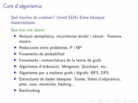
Curs d’algorısmia:

Que haurıeu de coneixer? (nivell EDA) Eines basiquesmatematiques

Que heu vist abans:

I Notacio asimptotica, recurrencies dividir i vencer: Teoremamestre.

I Reduccions entre problemes, P i NP

I Fonaments de probabilitat

I Fonaments i nomenclatura de la teoria de grafs

I Algorismes d’ordenacio: Mergesort, Quicksort, etc..

I Algorismes per a explorar grafs i digrafs: BFS, DFS.

I Estructures de dades basiques: Taules, llistes d’adjacencia,piles, cues, monticles, hashing,..

I Backtraking

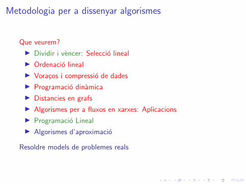
Metodologia per a dissenyar algorismes

Que veurem?

I Dividir i vencer: Seleccio lineal

I Ordenacio lineal

I Voracos i compressio de dades

I Programacio dinamica

I Distancies en grafs

I Algorismes per a fluxos en xarxes: Aplicacions

I Programacio Lineal

I Algorismes d’aproximacio

Resoldre models de problemes reals

Bibliografia:

Referencies principals:

”The algorithmic lenses: C. Papadimitriou”

Theoretical computer Science views computation as a ubiquitous

phenomenon, not one that it is limited to computers.

In 1936 Alan Turing demonstrated the universality of computational

principles with his mathematical model of the Turing machine.

Today’s algorithms represent a new way to study problems and events in

different individual and collective developments in humanity.

Algorithms themselves have evolved into a complex set of techniques, for

instances self-learning , Web services, concurrent, distributed or parallel,

etc... Each of them with ad-hoc relevant computational limitations and

social implications.

However, this course will be a course on classical algorithms, which are

the core needed to understand more advanced computational material.

Algorithms.

Great algorithms are the poetry of computation. As verse, they can be

terse, elusive and mysterious. But once unlocked, they cast a brilliant

new light on some aspects of computing. Francis Sullivan

Algorithm: Precise recipe for a precise computational task, whereeach step of the process must be clear and unambiguous, and itshould always yield a clear answer.

Sqrt (n)x0 = 1 y0 = nfor i = 1 to 6 do

yi = (xi−1 + yi−1)/2xi = n/yi

end for

Babilonia (XVI BC)

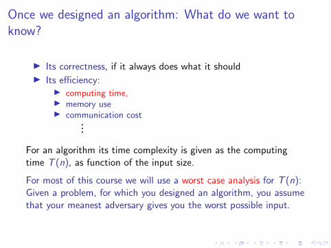
Once we designed an algorithm: What do we want toknow?

I Its correctness, if it always does what it shouldI Its efficiency:

I computing time,I memory useI communication cost

...

For an algorithm its time complexity is given as the computingtime T (n), as function of the input size.

For most of this course we will use a worst case analysis for T (n):Given a problem, for which you designed an algorithm, you assumethat your meanest adversary gives you the worst possible input.

Important

The time complexity must be independent of the ”used” machine

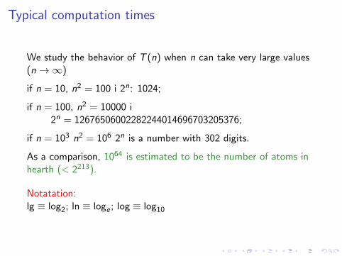
Typical computation times

We study the behavior of T (n) when n can take very large values(n→∞)

if n = 10, n2 = 100 i 2n: 1024;

if n = 100, n2 = 10000 i2n = 12676506002282244014696703205376;

if n = 103 n2 = 106 2n is a number with 302 digits.

As a comparison, 1064 is estimated to be the number of atoms inhearth (< 2213).

Notatation:lg ≡ log2; ln ≡ loge ; log ≡ log10

almost.

Typical computation times

We study the behavior of T (n) when n can take very large values(n→∞)

if n = 10, n2 = 100 i 2n: 1024;

if n = 100, n2 = 10000 i2n = 12676506002282244014696703205376;

if n = 103 n2 = 106 2n is a number with 302 digits.

As a comparison, 1064 is estimated to be the number of atoms inhearth (< 2213).

Notatation:lg ≡ log2; ln ≡ loge ; log ≡ log10 almost.

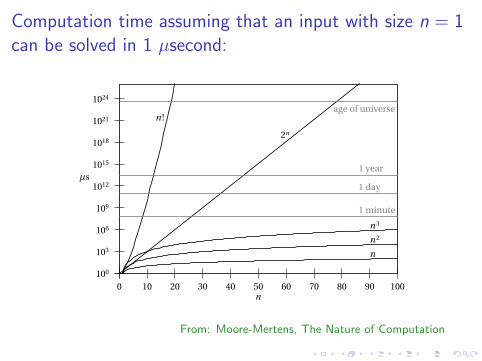
Computation time assuming that an input with size n = 1can be solved in 1 µsecond:26 THE BASICS

100

103

106

109

1012

1015

1018

1021

1024

0 10 20 30 40 50 60 70 80 90 100n

µs

n

n 2

n 3

2n

n !

1 minute

1 day

1 year

age of universe

FIGURE 2.5: Running times of algorithms as a function of the size n . We assume that each one can solvean instance of size n = 1 in one microsecond. Note that the time axis is logarithmic.

Eulerinput: a graph G = (V, E )output: “yes” if G is Eulerian, and “no” otherwisebegin

y := 0 ;for all v ∈V do

if deg(v ) is odd then y := y +1;if y > 2 then return “no”;

endreturn “yes”

end

FIGURE 2.6: Euler’s algorithm for EULERIAN PATH. The variable y counts the number of odd-degree vertices.

2.4.2 Details, and Why they Don’t Matter

In the Prologue we saw that Euler’s approach to EULERIAN PATH is much more efficient than exhaustivesearch. But how does the running time of the resulting algorithm scale with the size of the graph? It turnsout that a precise answer to this question depends on many details. We will discuss just enough of thesedetails to convince you that we can and should ignore them in our quest for a fundamental understandingof computational complexity.

From: Moore-Mertens, The Nature of Computation

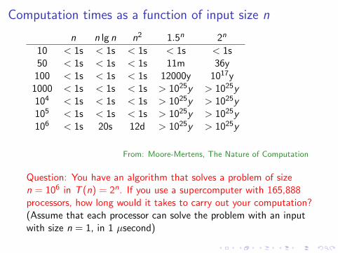
Computation times as a function of input size n

n n lg n n2 1.5n 2n

10 < 1s < 1s < 1s < 1s < 1s50 < 1s < 1s < 1s 11m 36y

100 < 1s < 1s < 1s 12000y 1017y1000 < 1s < 1s < 1s > 1025y > 1025y104 < 1s < 1s < 1s > 1025y > 1025y105 < 1s < 1s < 1s > 1025y > 1025y106 < 1s 20s 12d > 1025y > 1025y

From: Moore-Mertens, The Nature of Computation

Question: You have an algorithm that solves a problem of sizen = 106 in T (n) = 2n. If you use a supercomputer with 165,888processors, how long would it takes to carry out your computation?(Assume that each processor can solve the problem with an inputwith size n = 1, in 1 µsecond)

Efficient algorithms and practical algorithms

Notice n1010

is a polynomial, but their computing time could beprohibitive.

In the same way, if we have cn2 for constant c = 1064, then cdominates inputs up to a size of n > 1064.In this course we will not enter in the analysis up to constants, butkeep in mind that constants matter!!!!

When analyzing an algorithm, we say it is feasible if it is poly time,otherwise it is say to be unfeasible.

In practice, even for feasible algorithms with time complexity of forexample n4, it could be slow for ”real” values of n ≥ 100.

Asymptotic notation

Symbol L = limn→∞f (n)g(n) intuition

f (n) = O(g(n)) L <∞ f ≤ g

f (n) = Ω(g(n)) L > 0 f ≥ g

f (n) = Θ(g(n)) 0 < L <∞ f = g

f (n) = o(g(n)) L = 0 f < g

f (n) = ω(g(n)) L =∞ f > g

Names used for specific function classes

name definition

polylogarithmic f = O(logc n) for cte. c

polynomial f = O(nc) for cte. c or nO(1)

subexponential f = o(2nε) ∀1 > ε > 0

exponential f = 2poly(n)

double exponential f = 2exp(n)

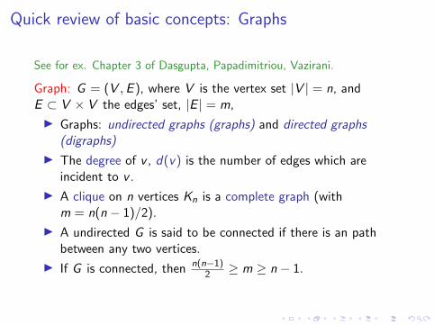
Quick review of basic concepts: Graphs

See for ex. Chapter 3 of Dasgupta, Papadimitriou, Vazirani.

Graph: G = (V ,E ), where V is the vertex set |V | = n, andE ⊂ V × V the edges’ set, |E | = m,

I Graphs: undirected graphs (graphs) and directed graphs(digraphs)

I The degree of v , d(v) is the number of edges which areincident to v .

I A clique on n vertices Kn is a complete graph (withm = n(n − 1)/2).

I A undirected G is said to be connected if there is an pathbetween any two vertices.

I If G is connected, then n(n−1)2 ≥ m ≥ n − 1.

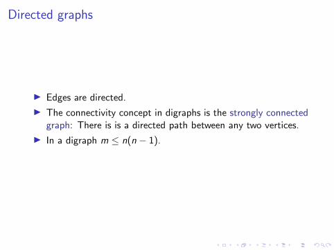
Directed graphs

I Edges are directed.

I The connectivity concept in digraphs is the strongly connectedgraph: There is is a directed path between any two vertices.

I In a digraph m ≤ n(n − 1).

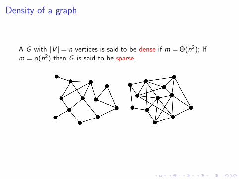
Density of a graph

A G with |V | = n vertices is said to be dense if m = Θ(n2); Ifm = o(n2) then G is said to be sparse.

Data structure for store graphs that you should know.

Let G be a graph with V = 1, 2, . . . , n. The two ways ofrepresenting G that you should know are:

Adjacency list

Adjacency matrix

Adjacency list

c

a

b

c

d

b d

a d c

d b

a b c

a

a

b

b c

d

d

c

a

b

c

d

a

b

d

c

Adjacency matrix

Given G with |V | = n define its adjacency matrix as the n × nmatrix:

A[i , j ] =

1 if (i , j) ∈ E ,

0 if (i , j) 6∈ E .

c

a

a

b

b c

d

d

abcd

a b c d0 1 0 11 0 1 10 1 0 11 1 1 0

abcd

a b c d0 0 0 11 0 1 00 0 0 00 1 1 0

Adjacency matrix

I If G is undirected, its adjacency matrix A(G ) is symmetric.

I If A is the adjacency matrix of G , then A2 the for i , j ∈ V ai ,jgives if there is a path between i and j in G , with length 2 .For any k > 0, ai ,j in Ak indicates if there is a path withlength k in G .

I If G has weights on edges, i.e. wi ,j for each (i , j) ∈ E , A(G )has wij in ai ,j .

I The use of the adjacency matrix allows the use of thepowerful tools from the matrix algebra.

Comparison between the use of the matrix representationand the list representation of G

I The use of adjacency list uses a single register per vertex anda single register per edge. As each register needs 2× 64 bits,then the space to represent a graph is Θ(n + m).

I The use of the adjacency matrix needs n2 bits (0, 1), so forunweighted graph G , we need Θ(n2) bits. For weighted G , weneed 64n2 bits (assuming weights are reasonably “small”).

I In general, for unweighted dense graphs, the adjacency matrixis better, otherwise the adjacency list is a shorterrepresentation.

Complexity issues between matrix and list representations

I Adding a new edge to G : In both data structures we needΘ(1).

I Query if for u and v in V (G ) there is an edge (u, v) ∈ E (V ):For matrix representation: Θ(1); For list representation: O(n).

I Explore all neighbours of vertex v : For matrix representation:Θ(n); For list representation: Θ(|d(v)|)

I Erase an edge in G In both data structures we need to make aQuery.

I Erase a vertex in G : For matrix representation: Θ(n); For listrepresentation: O(m).

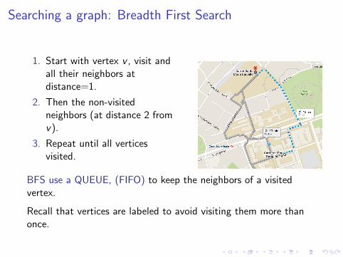
Searching a graph: Breadth First Search

1. Start with vertex v , visit andall their neighbors atdistance=1.

2. Then the non-visitedneighbors (at distance 2 fromv).

3. Repeat until all verticesvisited.

BFS use a QUEUE, (FIFO) to keep the neighbors of a visitedvertex.

Recall that vertices are labeled to avoid visiting them more thanonce.

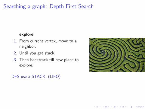
Searching a graph: Depth First Search

explore

1. From current vertex, move to aneighbor.

2. Until you get stuck.

3. Then backtrack till new place toexplore.

DFS use a STACK, (LIFO)

Time Complexity of DFS and BFS

For graphs given by adjacency lists:

O(|V |+ |E |)

For graphs given by adjacency matrix:

• DFS and • BFS: O(|V |2)

Therefore, both procedures can be implemented in linear time withrespect to the size of the input graph.

Connected components in undirected graphs.

A connected component is a maximal connected subgraph of G .

A connected graph has a unique connected component.

Connected ComponentsINPUT: undirected graph GQUESTION: Find all the connected components of G .

To find connected components in Guse DFS and keep track of the set ofvertices visited in each explore call.

C

D

G

H

A F

L K

E

IJ

B

The problem can be solved in O(|V |+ |E |).

Strongly connected components in a digraph

Kosharaju-Sharir’s algorithm: Uses BFS (twice). ComplexityT (n) = O(|V |+ |E |)

Tarjan’s algorithm: Based in using DFS. ComplexityT (n) = O(|V |+ |E |)

Both algorithms are optimal, i.e. are lineal, but in practice Tarjan’salgorithm is easier to implement.

A nice property: Every digraph has a directed acyclic graph (dag)on its strongly connected components.

K

A B C

D E F

HGI

J L

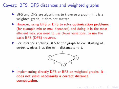
Caveat: BFS, DFS distances and weighted graphs

I BFS and DFS are algorithms to traverse a graph, if it is aweighted graph, it does not matter.

I However, using BFS or DFS to solve optimization problems(for example min or max distances) and doing it in the mostefficient way, you need to use clever variations, to use thebasic BFS (DFS) traverse.

I For instance applying BFS to the graph below, starting atvertex s, gives 3 as the min. distance s → t:

1

s

a

t

3

1

I Implementing directly DFS or BFS on weighted graphs, itdoes not yield necessarily a correct distancecomputation.

The classes P and NP

I Recall a problem belong to the class P if there exists analgorithm that is polynomial in the worst-case analysis, (forthe worst input given by a malicious adversary)

I A problem given in decisional form belong to the class NPnon-deterministic polynomial time if given a certificate of asolution we can verify in polynomial time that indeed thecertificate is a valid solution to the problem in decisional form.

I It is easy to se that P⊆ NP, but it is an open problem toprove that P=NP or that P6=NP.

I The class NP-complete are the class of most difficult problemsin decisional form that are in NP. Most difficult in the sensethat if one of them is proved to be in P then P=NP.

Beyond worst-case analysis

I Under the hypothesis that P 6=NP, if the decision version of aproblem is in NP-complete, then the optimization problem willrequire at least exponential time, for some inputs.

I The classification of a problem as NP-complete is a case ofworst-case analysis, and for many problems the ”expensiveinputs” are few, and far from practical typical inputs. We willsee some examples through the course, as the knapsack.

I Therefore, there are alternative ways to get in practice,solutions for NP-complete problems, with the use ofalternative algorithmic techniques, as approximation (we willsee some examples), heuristics and self-learning algorithms,that are deferred to other courses.

A powerful tool to solve problems: Bounded Reductions

You have been introduced in previous courses to the concept ofreduction between decision problems, to define the classNP-complete. We can extend the concept to function problems:

Given problems A and B, assume we have an algorithm AB tosolve the problem B on any input y .A polynomial time a reduction A ≤ B is a polynomial timecomputable function f that for any input x for A, in polynomialtime transform it into a specific input f (x) for problem B such thatx has a valid solution for A iff f (x) has a valid solution for B.

Therefore if we have that A ≤ B, as there is an algorithm AB tosolve problem B, then we have an algorithm AA for any input x ofA: Compute AB(f (x)).

If B is in P, i.e. for every input y of B, AB(y) yields an answer inpolynomial time, then AA(x) = AB(f (x)) also is a polynomialtime algorithm for A, so A ∈ P.

The Vertex Cover problem

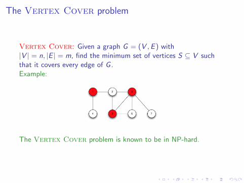
Vertex Cover: Given a graph G = (V ,E ) with|V | = n, |E | = m, find the minimum set of vertices S ⊆ V suchthat it covers every edge of G .Example:

The Vertex Cover problem is known to be in NP-hard.

The Set Cover problem

Set Cover: Given a set U of m elements, a collectionS = S1, . . . ,Sn where each Si ⊆ U, find the minimal number ofsubsets whose union is equal to U.

There also is a weighted version, but the simpler version already isNP-hard.

Example: Given U = 1, 2, 3, 4, 5, 6, 7 (m = 7), with Sa = 3, 7,Sb = 2, 4, Sc = 3, 4, 5, 6, Sd = 5, Se = 1, Sf = 1, 2, 6, 7.

Solution: Sc , Sf U

1 2

5

6

4

37

Set Cover

The Vertex Cover problem is a special case of the Set Coverproblem. As a model, the Set Cover has important practicalapplications.To understand the computational complexity of Set Cover it isimportant to understand first the complexity of special cases asVertex Cover.

An example of Set Cover as a model: A software company hasa list of 5000 computer viruses (U), consider the 9000 sets formedby substrings of 20 or more consecutive bytes from viruses. Wewant to check for the existence of those bytes of viruses in ourdeveloped code. If we can find a small set cover, say 180substrings, then it suffices to search for these 180 substrings toverify the existence of known computer viruses.

Vertex Cover ≤ Set Cover

Given a input to Vertex Cover G = (V ,E ), of size|V |+ |E | = n + m we want to construct in polynomial time onn + m a specific input f (G ) = (U, S) to Set Cover such that ifthere exist a polynomial algorithm A to find a min. vertex cover inG , then A(f (G )) is an efficient algorithm to find an optimalsolution to set cover.

REDUCTION f :

I Consider U as the set E of edges.

I For each vertex i ∈ V , Si is the set of edges incident to i .Therefore |S | = n and for each Si , |Si | ≤ m.

I The cost of the reduction from G to (U,S) is O(m + nm)

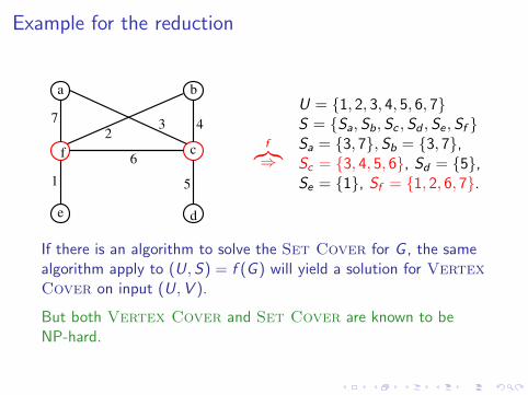
Example for the reduction

7

a b

c

de

f

1

23 4

5

6

f︷︸︸︷⇒U = 1, 2, 3, 4, 5, 6, 7S = Sa,Sb,Sc , Sd ,Se , Sf Sa = 3, 7, Sb = 3, 7,Sc = 3, 4, 5, 6, Sd = 5,Se = 1, Sf = 1, 2, 6, 7.

Example for the reduction

7

a b

c

de

f

1

23 4

5

6

f︷︸︸︷⇒U = 1, 2, 3, 4, 5, 6, 7S = Sa,Sb,Sc , Sd ,Se , Sf Sa = 3, 7, Sb = 3, 7,Sc = 3, 4, 5, 6, Sd = 5,Se = 1, Sf = 1, 2, 6, 7.

If there is an algorithm to solve the Set Cover for G , the samealgorithm apply to (U,S) = f (G ) will yield a solution for VertexCover on input (U,V ).

But both Vertex Cover and Set Cover are known to beNP-hard.

Some math. you should remember

Given an integer n > 0 and a real a > 1 and a 6= 0:

I Arithmetic summation:∑n

i=0 i = n(n+1)2 .

I Geometric summation:∑n

i=0 ai = 1−an+1

1−a .

Logarithms and Exponents: For a, b, c ∈ R+,

I logb a = c ⇔ a = bc ⇒ logb 1 = 0

I logb ac = logb a + logb c , logb a/c = logb a− logb c .

I logb ac = c logb a ⇒ c logb a = alogb c ⇒ 2log2 n = n.

I logb a = logc a/ logc b ⇒ logb a = Θ(logc a)

Stirling: n! =√

2πn(n/e)n + 0(1/n) + γ ⇒ n! + ω((n/2)n).

n-Harmonic: Hn =∑n

i=1 1/i ∼ ln n.

The divide-and-conquer strategy.

1. Break the problem into smallersubproblems,

2. recursively solve each problem,

3. appropriately combine theiranswers. Julius Caesar (I-BC)

”Divide et impera”

Known Examples:

I Binary search

I Merge-sort

I Quicksort

I Strassen matrix multiplication

J. von Neumann(1903-57)Merge sort

Recurrences Divide and Conquer

T (n) = 3T (n/2) + O(n)The algorithm under analysis divides input of size n into 3subproblems, each of size n/2, at a cost (of dividing and joiningthe solutions) of O(n)

n/4

1 1 1 1 1 1

size n

n/2n/2n/2

n/4 n/4 n/4 n/4 n/4 n/4 n/4 n/4

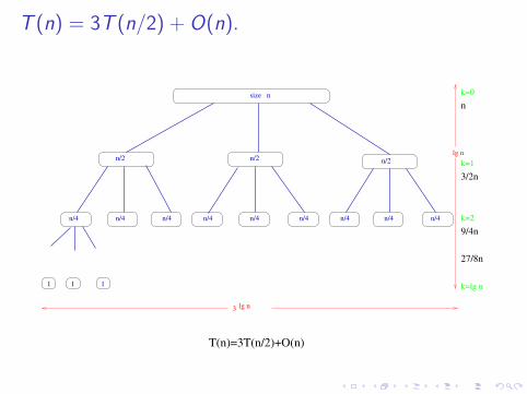
T (n) = 3T (n/2) + O(n).

3

1 1 1

k=0

k=1

k=2

k=lg n

lg n

size n

T(n)=3T(n/2)+O(n)

n/2 n/2 n/2

n/4 n/4

27/8n

9/4n

3/2n

n

n/4 n/4 n/4

lg n

n/4n/4n/4n/4

At depth k of the tree there are 3k subproblems, each of size n/2k .

For each of those problems we need O(n/2k) (splitting time +combination time).Therefore the cost at depth k is:

3k ×( n

2k

)=

(3

2

)k

× O(n).

with max. depth k = lg n.(1 +

3

2+ (

3

2)2 + (

3

2)3 + · · ·+ (

3

2)lg n)

Θ(n)

Therefore T (n) =∑lg n

k=0O(n)(32)k .

From T (n) = O(n)

lg n∑k=0

(3

2)k︸ ︷︷ ︸

(∗)

,

We have a geometric series of ratio 3/2, starting at 1 and ending

at((32)lg n

)= nlg 3

nlg 2 = n1.58

n = n0.58.

As the series is increasing, T (n) is dominated by the last term:

T (n) = O(n)×(nlg 3

n

)= O(n1.58).

The Master Theorem

There are several versions of the Master Theorem to solve D&Crecurrences. The one presented below is taken from DPV’s book.A different one can be found in CLRS’s book Theorem 4.1

Theorem (DPV-2.2)

If T (n) = aT (dn/be) + O(nd) for constants a ≥ 1, b > 1, d ≥ 0,then has asymptotic solution:

T (n) =

O(nd), if d > logb a,

O(nd lg n), if d = logb a,

O(nlogb a), if d < logb a.

The basic M.T. leave many cases outside. For stronger MT:

Akra-Bazi Theorem: https:

//courses.csail.mit.edu/6.046/spring04/handouts/akrabazzi.pdf

Salvador Roura Theorems http://www.lsi.upc.edu/~diaz/RouraMT.pdf