Introducción al la programación en python: algunas ideas básicas

Cecilia Jarne

cecilia.jarne@unq.edu.ar

7 al 18 de Marzo @ DF UBACABA, Argentina

2

Ideas básicas de Python

Es un lenguaje multiparadigma:­ soporta orientación a objetos.­ programación imperativa.­ programación funcional.

Es  un  lenguaje  de  programación interpretado,  que  permite  tipado dinámico y es multiplataforma.

https://www.python.org

3

Ideas básicas de Python

 ¿Por qué aprender python si yo ya se programar en *****?

1)Fácil de aprender.2)Un conjunto gigante de librerías.3)Soporte científico excelente!!4)Se puede desarrollar software bastante rápido.5)Posee una licencia de código abierto.6)Una comunidad gigante desarrollando con la cual realmente se puede contar.

4

Ideas básicas de Python

Algo breve de historia...

­ Desarrollado desde 1989 por Guido van Rossum.

­ Versión Python 2.0: Octubre 2000 (now: 2.7.6)

­ Versión Python 3.0: Diciembre 2008 (now 3.3.5)

5

Ideas básicas de Python

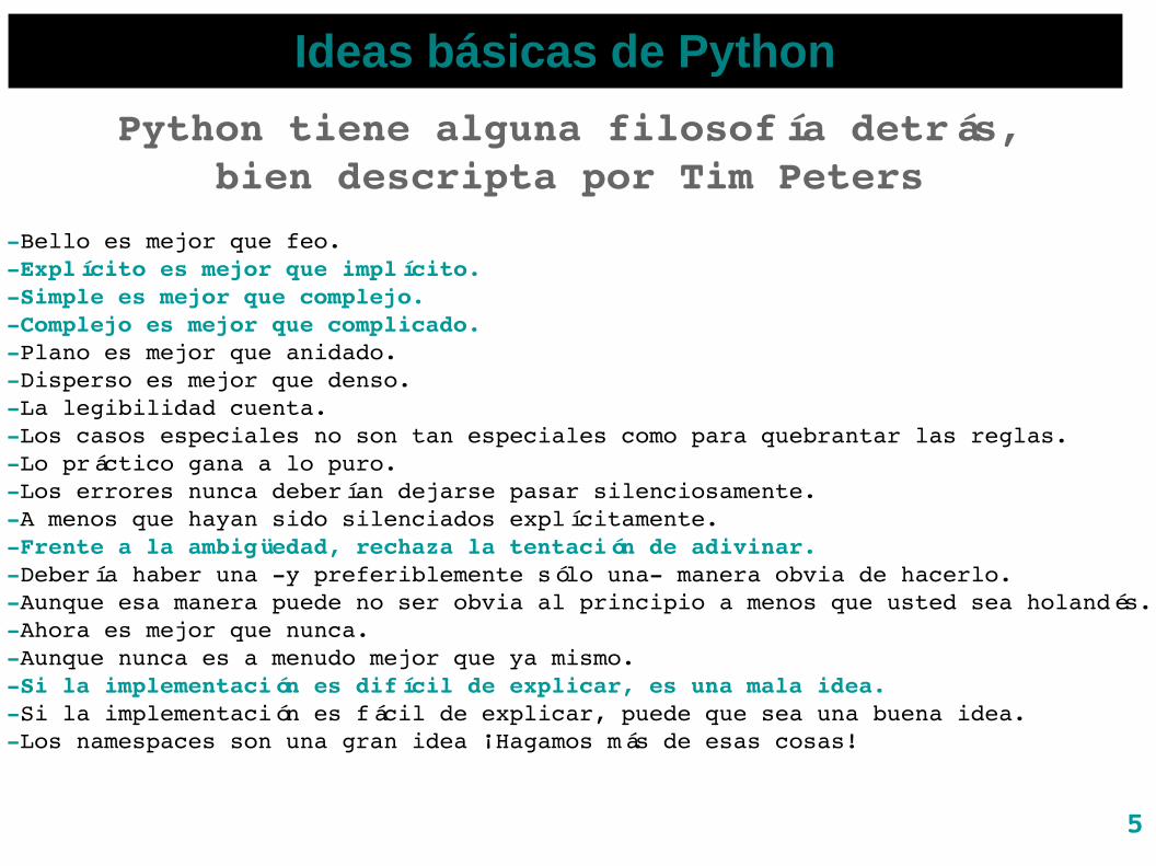
Python tiene alguna filosofía detrás, bien descripta por Tim Peters

­Bello es mejor que feo.­Explícito es mejor que implícito.­Simple es mejor que complejo.­Complejo es mejor que complicado.­Plano es mejor que anidado.­Disperso es mejor que denso.­La legibilidad cuenta.­Los casos especiales no son tan especiales como para quebrantar las reglas.­Lo práctico gana a lo puro.­Los errores nunca deberían dejarse pasar silenciosamente.­A menos que hayan sido silenciados explícitamente.­Frente a la ambigüedad, rechaza la tentación de adivinar.­Debería haber una ­y preferiblemente sólo una­ manera obvia de hacerlo.­Aunque esa manera puede no ser obvia al principio a menos que usted sea holandés.­Ahora es mejor que nunca.­Aunque nunca es a menudo mejor que ya mismo.­Si la implementación es difícil de explicar, es una mala idea.­Si la implementación es fácil de explicar, puede que sea una buena idea.­Los namespaces son una gran idea ¡Hagamos más de esas cosas!

6

Ideas básicas de Python

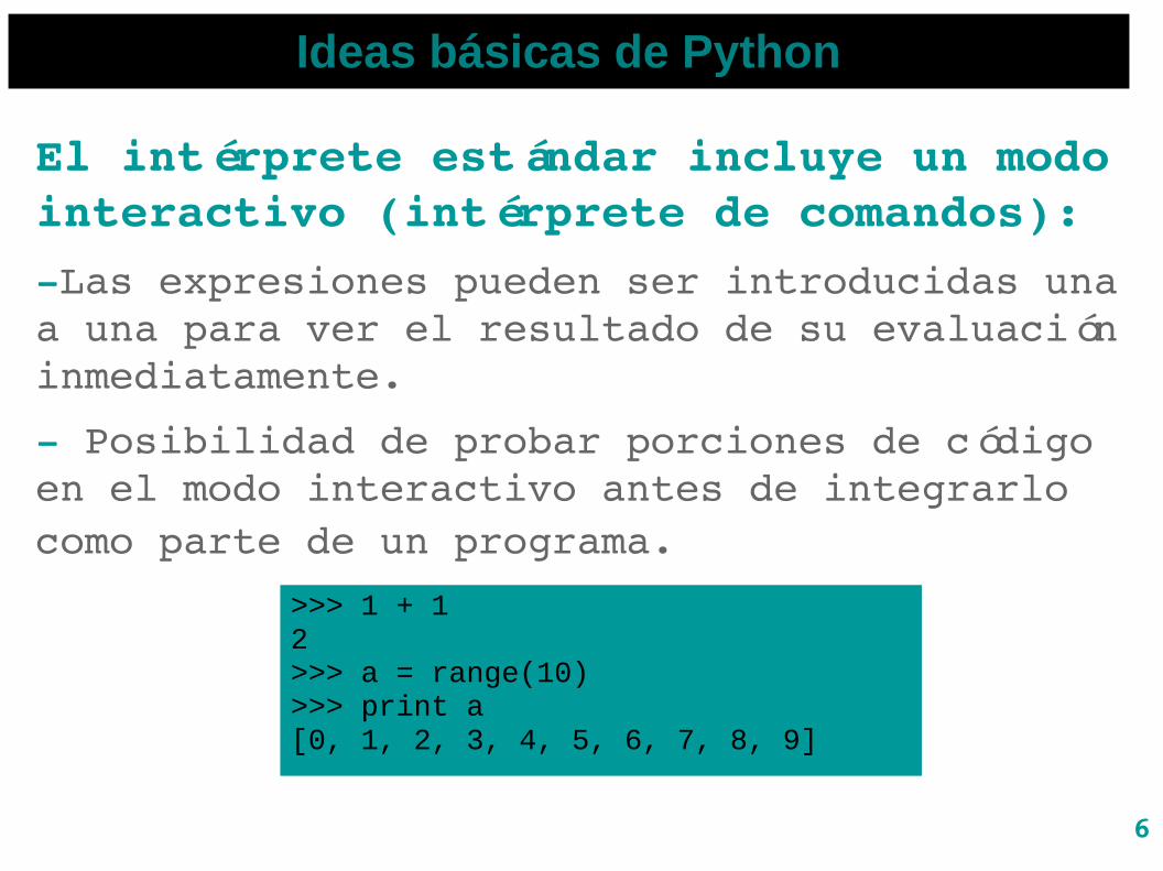
El intérprete estándar incluye un modo interactivo (intérprete de comandos): ­Las expresiones pueden ser introducidas una a una para ver el resultado de su evaluación inmediatamente.

­ Posibilidad de probar porciones de código en el modo interactivo antes de integrarlo como parte de un programa. 

>>> 1 + 12>>> a = range(10)>>> print a[0, 1, 2, 3, 4, 5, 6, 7, 8, 9]

7

Ideas básicas de Python

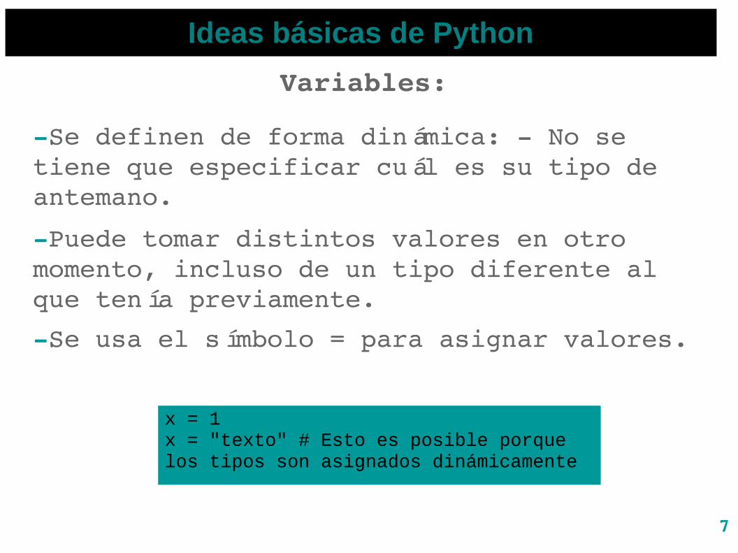
­Se definen de forma dinámica: ­ No se tiene que especificar cuál es su tipo de antemano.

­Puede tomar distintos valores en otro momento, incluso de un tipo diferente al que tenía previamente.

­Se usa el símbolo = para asignar valores.

x = 1x = "texto" # Esto es posible porque los tipos son asignados dinámicamente

Variables:

8

Ideas básicas de Python

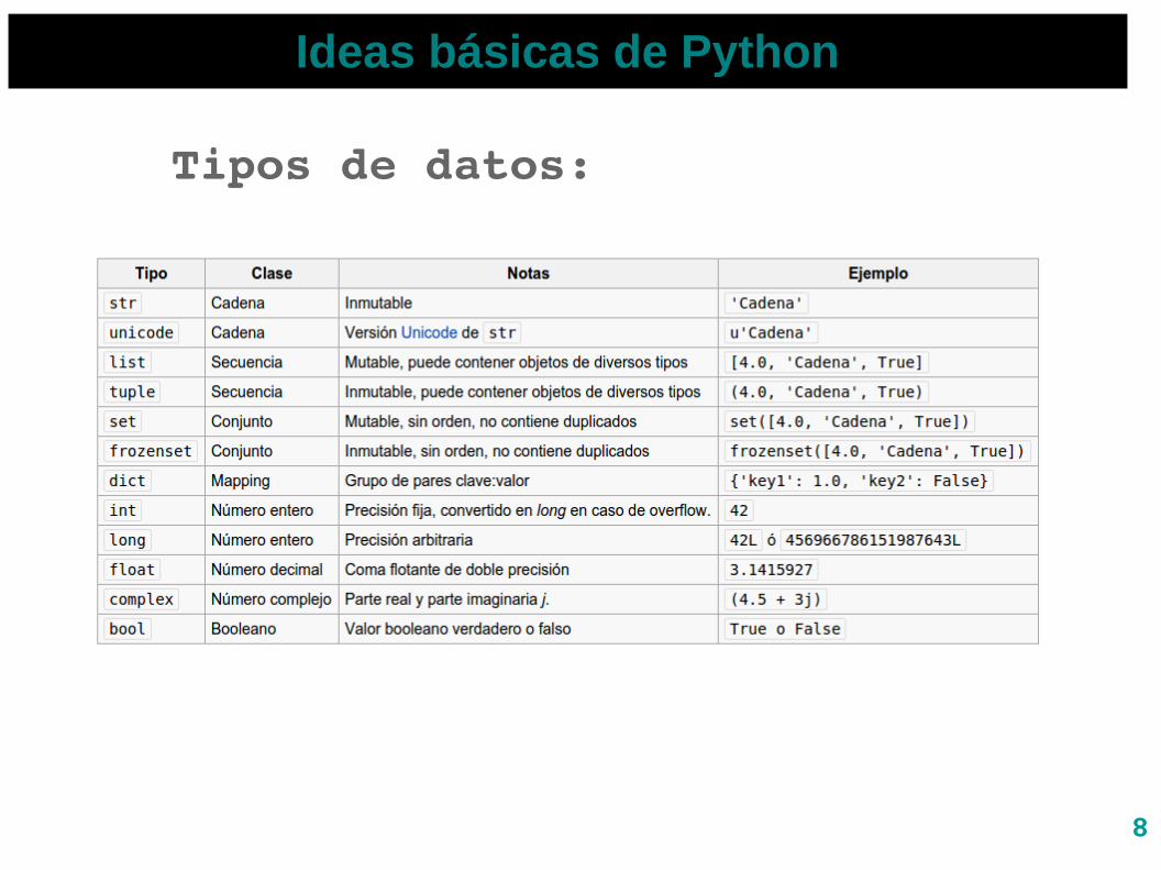
 Tipos de datos:

9

Ideas básicas de Python

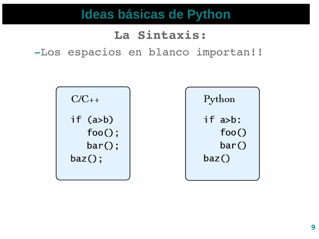
­Los espacios en blanco importan!!

La Sintaxis:

10

Ideas básicas de Python

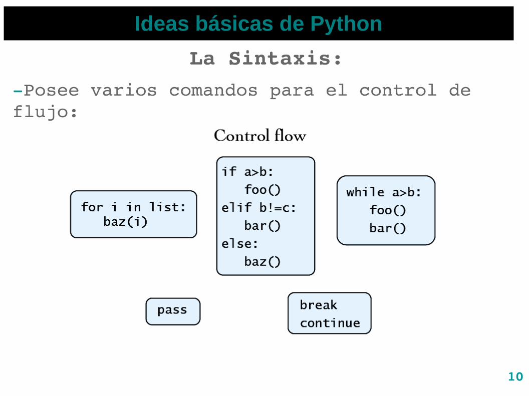
­Posee varios comandos para el control de flujo:

La Sintaxis:

11

Ideas básicas de Python

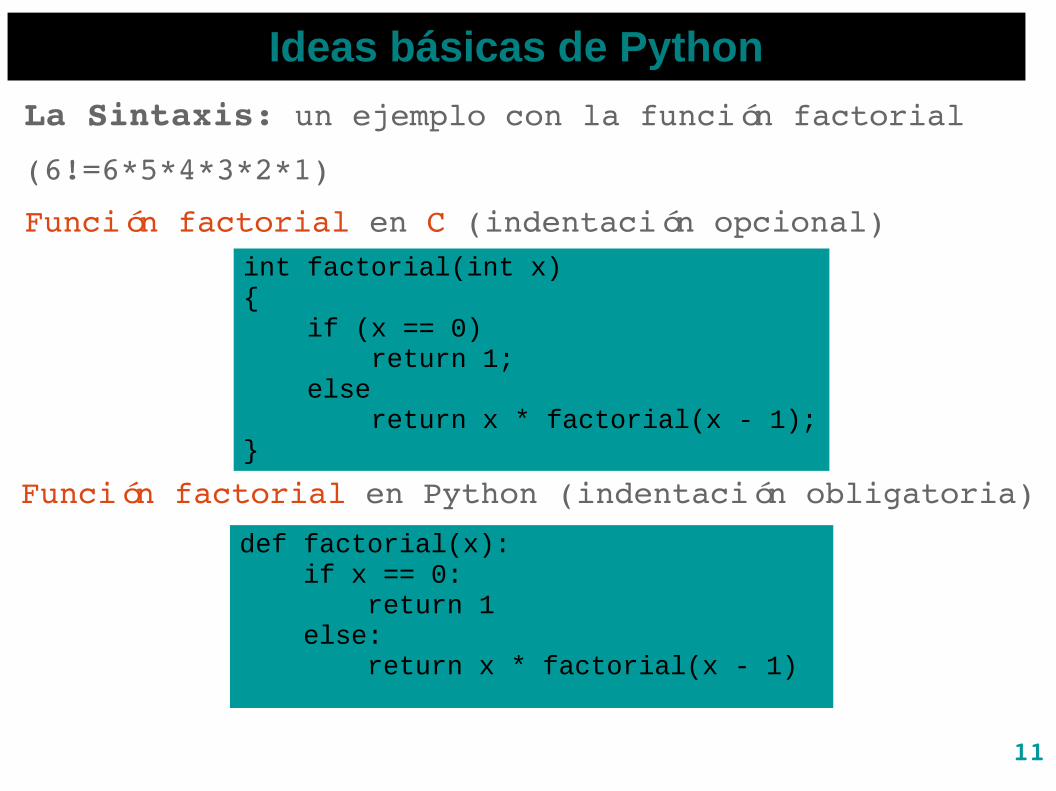
La Sintaxis: un ejemplo con la función factorial 

(6!=6*5*4*3*2*1)

int factorial(int x){ if (x == 0) return 1; else return x * factorial(x - 1);}

def factorial(x): if x == 0: return 1 else: return x * factorial(x - 1)

Función factorial en C (indentación opcional)

Función factorial en Python (indentación obligatoria)

12

Ideas básicas de Python

La Sintaxis:

­Las funciones pueden ser pasadas como valores!

13

Ideas básicas de Python

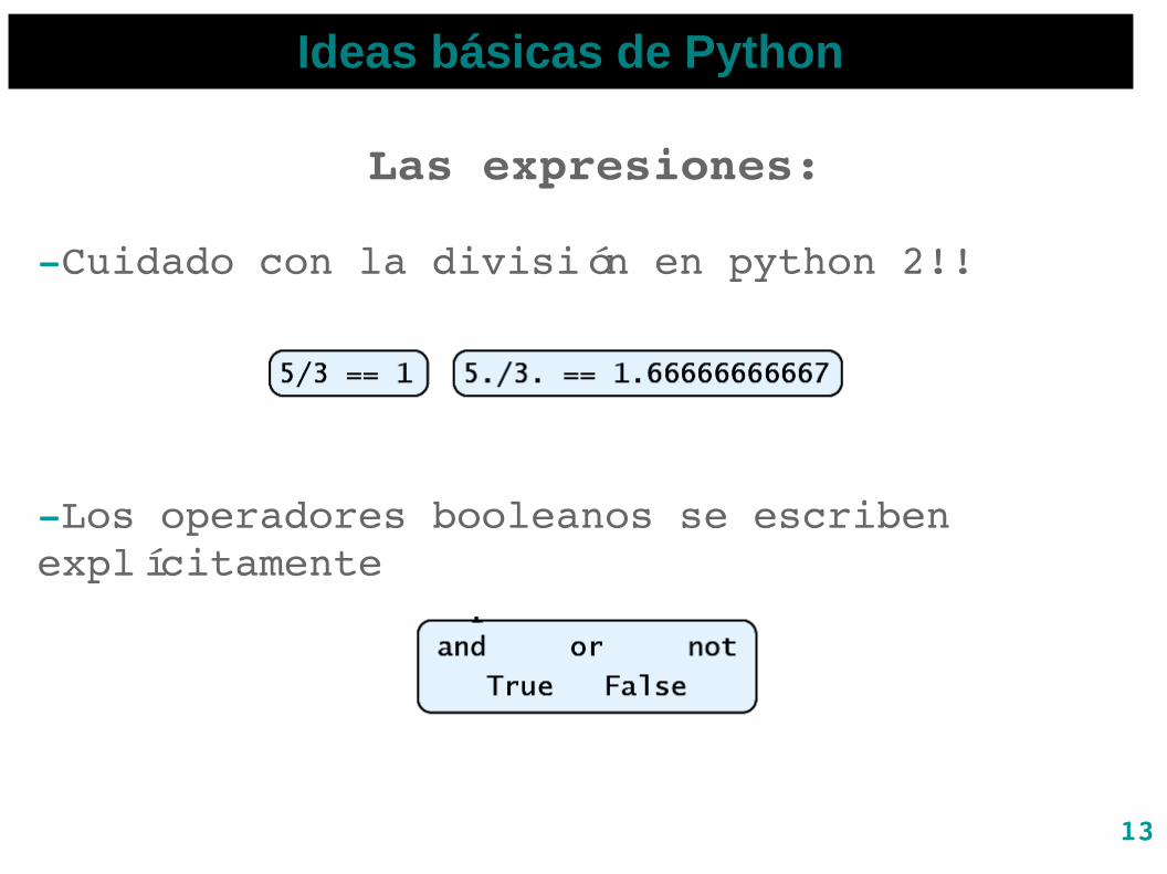
Las expresiones:

­Cuidado con la división en python 2!!

­Los operadores booleanos se escriben explícitamente

14

Ideas básicas de Python

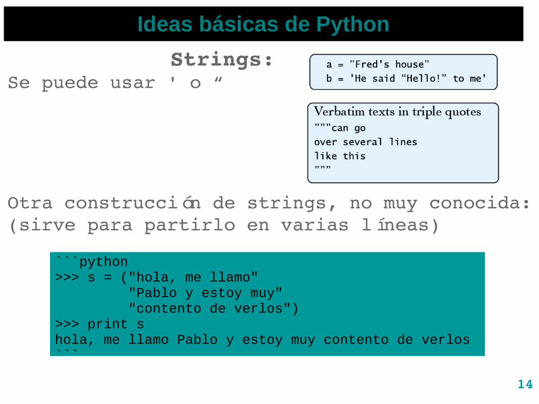
Strings:Se puede usar ' o “

Otra construcción de strings, no muy conocida: (sirve para partirlo en varias líneas)

```python>>> s = ("hola, me llamo" "Pablo y estoy muy" "contento de verlos")>>> print shola, me llamo Pablo y estoy muy contento de verlos```

15

Ideas básicas de Python

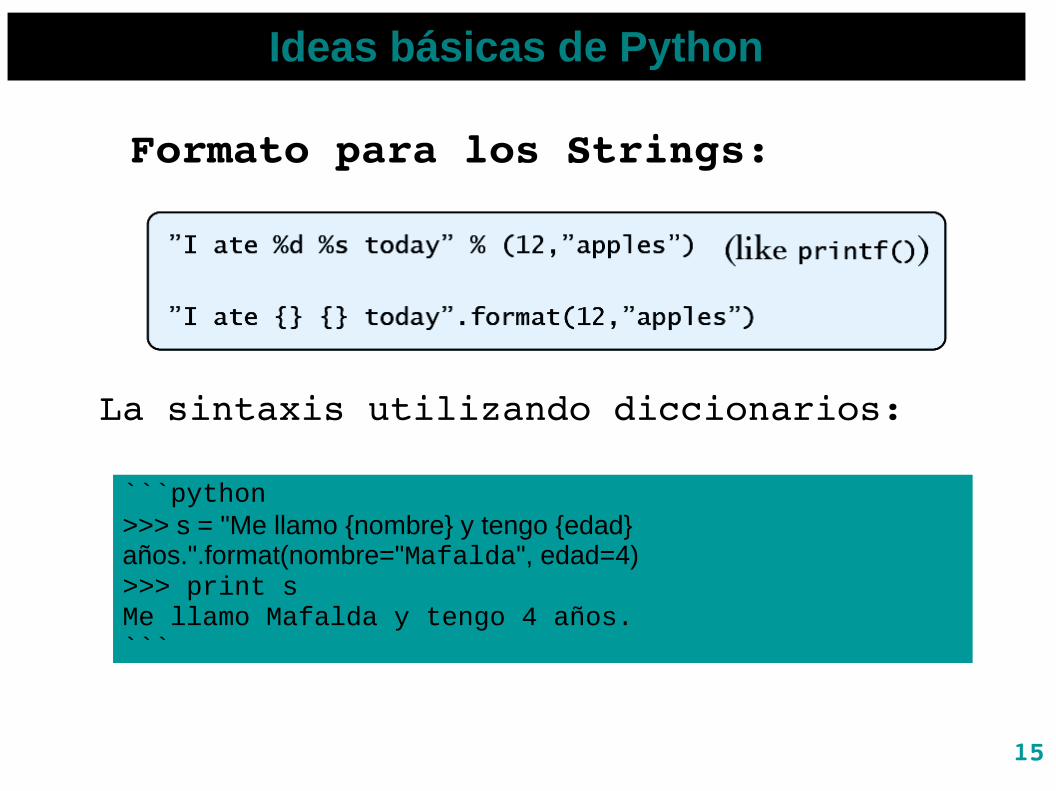
Formato para los Strings:

```python>>> s = "Me llamo {nombre} y tengo {edad} años.".format(nombre="Mafalda", edad=4)>>> print sMe llamo Mafalda y tengo 4 años.```

 La sintaxis utilizando diccionarios:

16

Ideas básicas de Python

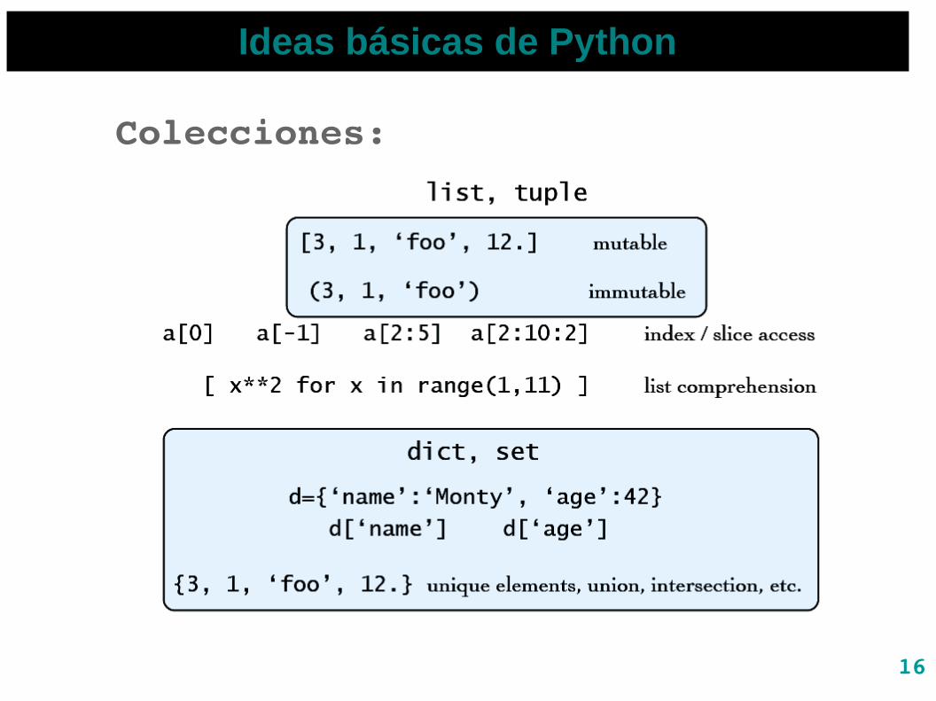
Colecciones:

17

Ideas básicas de Python

Si aun la motivación no alcanza, aquí la verdadera razón de porqué me convertí a python:

NumPy: http://www.numpy.org/

SciPy:http://www.scipy.org/

MatPlotLib:http://matplotlib.org/

18

Ideas básicas de Python

NumPy: 

Es un paquete fundamental para python de programación cientifica. Entre otras cosas contiene:

­Potentes arrays N­dimensionales.­Funciones sofisticadas.­Herramientas para integración con código C/C++ y Fortran.­Herramientas útiles de alegra lineal, transformada de fourier, y generadores de números aleatorios.

19

Ideas básicas de Python

SciPy: 

Es un paquete que extiende la funcionalidad de  Numpy  con  una  colección  substancial  de algoritmos  por  ejemplo  de  minimización,   cálculo y procesamiento de señales.

20

Ideas básicas de Python

Es una librería de python para gráficos 2D que produce imágenes de alta calidad en una gran diversidad de formatos y entornos o 

plataformas interactivas. 

­Puede ser usada en scrips de python o en entorno interactivo al estilo de  MATLAB®* or Mathematica® y también e aplicaciones web.

­Por supuesto también es open source!!! 

MatPlotlib: 

21

Ideas básicas de Python

Para poder utilizar estas librerías hay que importarlas:

22

Ideas básicas de Python

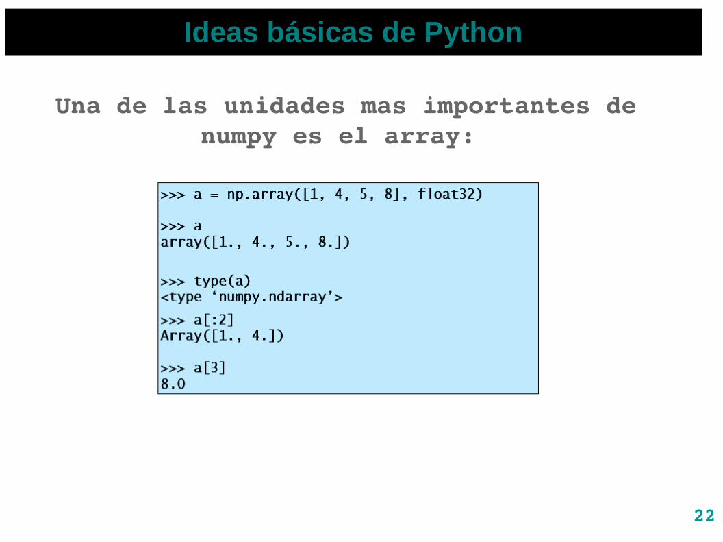
Una de las unidades mas importantes de numpy es el array: 

23

Ideas básicas de Python

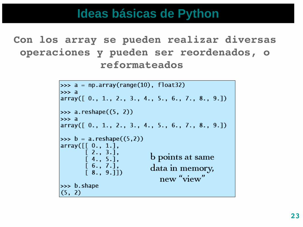
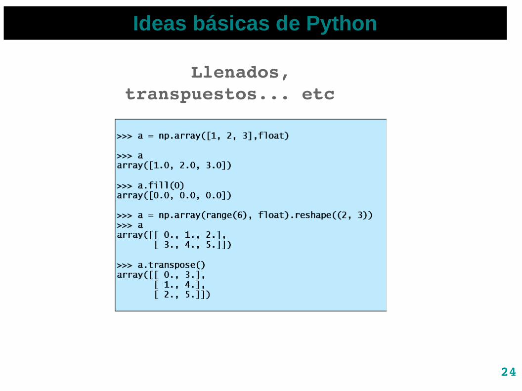
Con los array se pueden realizar diversas operaciones y pueden ser reordenados, o 

reformateados 

24

Ideas básicas de Python

Llenados, transpuestos... etc  

25

Ideas básicas de Python

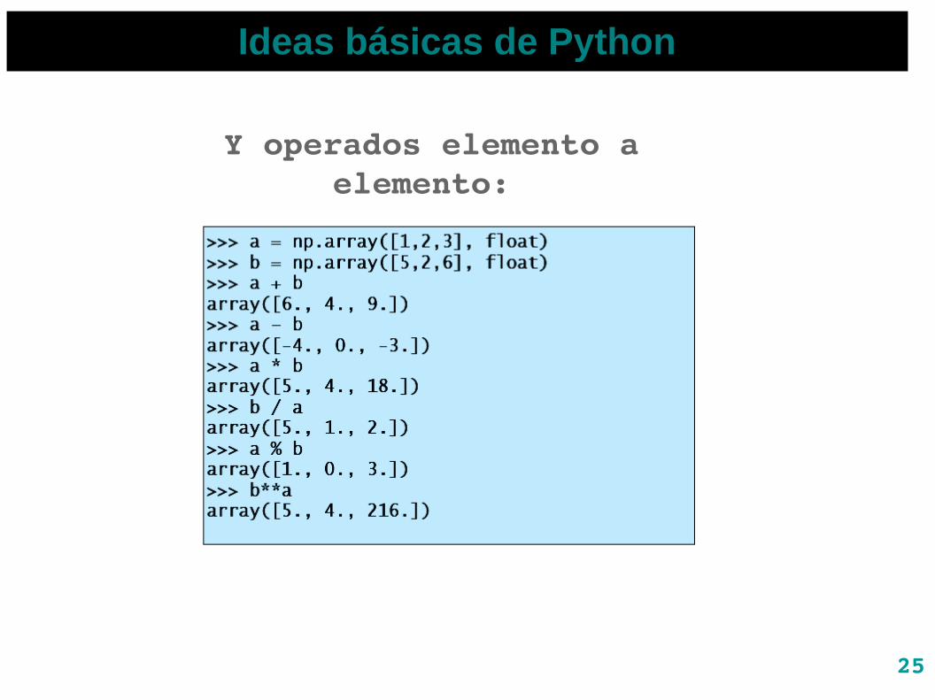
Y operados elemento a elemento: 

26

Ideas básicas de Python

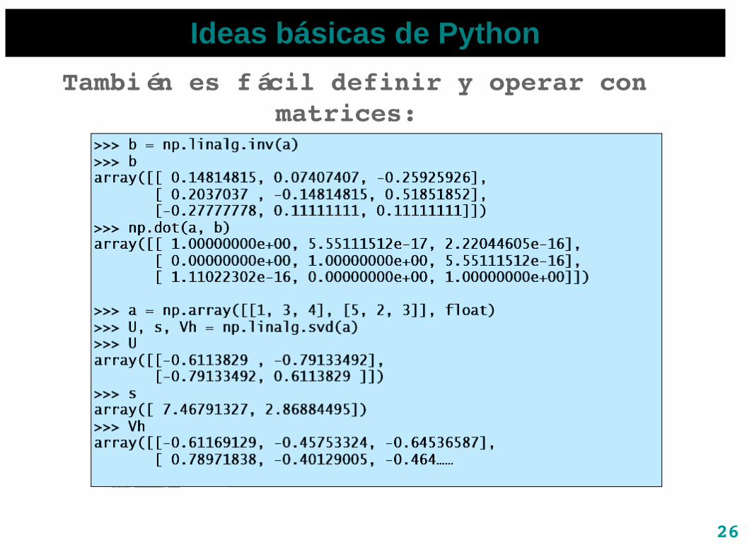
También es fácil definir y operar con matrices: 

27

Ideas básicas de Python

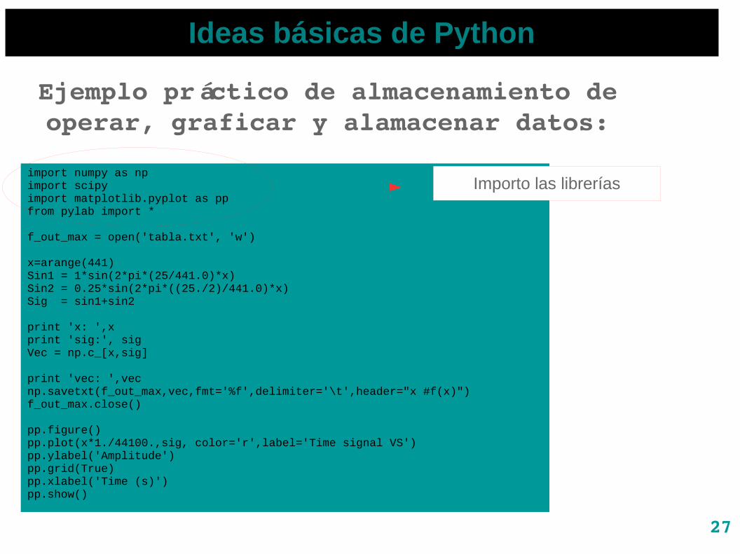
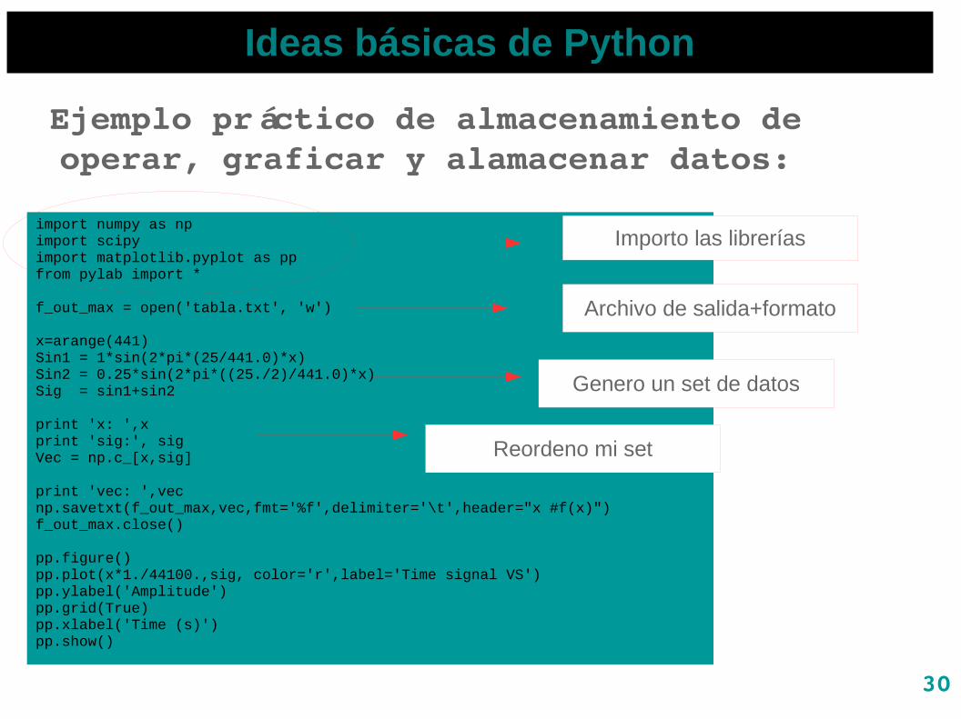
Ejemplo práctico de almacenamiento de operar, graficar y alamacenar datos:

import numpy as npimport scipyimport matplotlib.pyplot as ppfrom pylab import *

f_out_max = open('tabla.txt', 'w')

x=arange(441)Sin1 = 1*sin(2*pi*(25/441.0)*x)Sin2 = 0.25*sin(2*pi*((25./2)/441.0)*x)Sig = sin1+sin2

print 'x: ',xprint 'sig:', sigVec = np.c_[x,sig]

print 'vec: ',vecnp.savetxt(f_out_max,vec,fmt='%f',delimiter='\t',header="x #f(x)") f_out_max.close()

pp.figure()pp.plot(x*1./44100.,sig, color='r',label='Time signal VS')pp.ylabel('Amplitude')pp.grid(True)pp.xlabel('Time (s)')pp.show()

Importo las librerías

28

import numpy as npimport scipyimport matplotlib.pyplot as ppfrom pylab import *

f_out_max = open('tabla.txt', 'w')

x=arange(441)Sin1 = 1*sin(2*pi*(25/441.0)*x)Sin2 = 0.25*sin(2*pi*((25./2)/441.0)*x)Sig = sin1+sin2

print 'x: ',xprint 'sig:', sigVec = np.c_[x,sig]

print 'vec: ',vecnp.savetxt(f_out_max,vec,fmt='%f',delimiter='\t',header="x #f(x)") f_out_max.close()

pp.figure()pp.plot(x*1./44100.,sig, color='r',label='Time signal VS')pp.ylabel('Amplitude')pp.grid(True)pp.xlabel('Time (s)')pp.show()

Ideas básicas de Python

Ejemplo práctico de almacenamiento de operar, graficar y alamacenar datos:

Importo las librerías

Archivo de salida+formato

29

import numpy as npimport scipyimport matplotlib.pyplot as ppfrom pylab import *

f_out_max = open('tabla.txt', 'w')

x=arange(441)Sin1 = 1*sin(2*pi*(25/441.0)*x)Sin2 = 0.25*sin(2*pi*((25./2)/441.0)*x)Sig = sin1+sin2

print 'x: ',xprint 'sig:', sigVec = np.c_[x,sig]

print 'vec: ',vecnp.savetxt(f_out_max,vec,fmt='%f',delimiter='\t',header="x #f(x)") f_out_max.close()

pp.figure()pp.plot(x*1./44100.,sig, color='r',label='Time signal VS')pp.ylabel('Amplitude')pp.grid(True)pp.xlabel('Time (s)')pp.show()

Ideas básicas de Python

Ejemplo práctico de almacenamiento de operar, graficar y alamacenar datos:

Importo las librerías

Archivo de salida+formato

Genero un set de datos

30

import numpy as npimport scipyimport matplotlib.pyplot as ppfrom pylab import *

f_out_max = open('tabla.txt', 'w')

x=arange(441)Sin1 = 1*sin(2*pi*(25/441.0)*x)Sin2 = 0.25*sin(2*pi*((25./2)/441.0)*x)Sig = sin1+sin2

print 'x: ',xprint 'sig:', sigVec = np.c_[x,sig]

print 'vec: ',vecnp.savetxt(f_out_max,vec,fmt='%f',delimiter='\t',header="x #f(x)") f_out_max.close()

pp.figure()pp.plot(x*1./44100.,sig, color='r',label='Time signal VS')pp.ylabel('Amplitude')pp.grid(True)pp.xlabel('Time (s)')pp.show()

Ideas básicas de Python

Ejemplo práctico de almacenamiento de operar, graficar y alamacenar datos:

Importo las librerías

Archivo de salida+formato

Genero un set de datos

Reordeno mi set

31

import numpy as npimport scipyimport matplotlib.pyplot as ppfrom pylab import *

f_out_max = open('tabla.txt', 'w')

x=arange(441)Sin1 = 1*sin(2*pi*(25/441.0)*x)Sin2 = 0.25*sin(2*pi*((25./2)/441.0)*x)Sig = sin1+sin2

print 'x: ',xprint 'sig:', sigVec = np.c_[x,sig]

print 'vec: ',vecnp.savetxt(f_out_max,vec,fmt='%f',delimiter='\t',header="x #f(x)") f_out_max.close()

pp.figure()pp.plot(x*1./44100.,sig, color='r',label='Time signal VS')pp.ylabel('Amplitude')pp.grid(True)pp.xlabel('Time (s)')pp.show()

Ideas básicas de Python

Ejemplo práctico de almacenamiento de operar, graficar y alamacenar datos:

Importo las librerías

Archivo de salida+formato

Genero un set de datos

Reordeno mi set

Guardo mi set en el outfile

32

import numpy as npimport scipyimport matplotlib.pyplot as ppfrom pylab import *

f_out_max = open('tabla.txt', 'w')

x=arange(441)Sin1 = 1*sin(2*pi*(25/441.0)*x)Sin2 = 0.25*sin(2*pi*((25./2)/441.0)*x)Sig = sin1+sin2

print 'x: ',xprint 'sig:', sigVec = np.c_[x,sig]

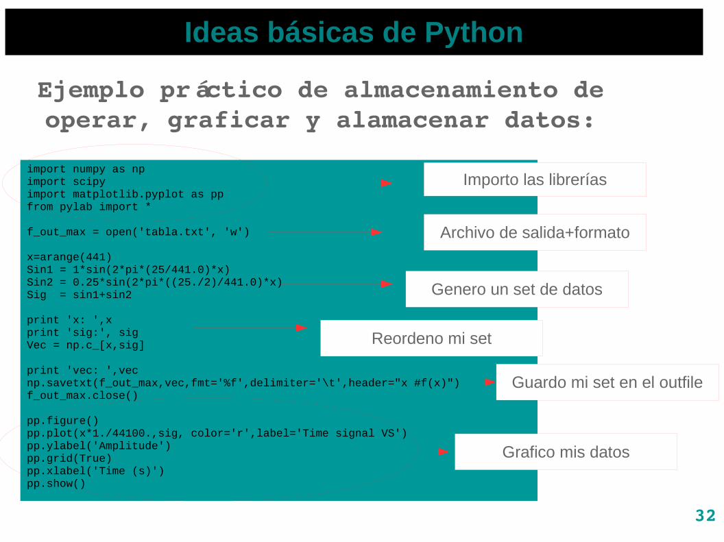
print 'vec: ',vecnp.savetxt(f_out_max,vec,fmt='%f',delimiter='\t',header="x #f(x)") f_out_max.close()

pp.figure()pp.plot(x*1./44100.,sig, color='r',label='Time signal VS')pp.ylabel('Amplitude')pp.grid(True)pp.xlabel('Time (s)')pp.show()

Ideas básicas de Python

Ejemplo práctico de almacenamiento de operar, graficar y alamacenar datos:

Importo las librerías

Archivo de salida+formato

Genero un set de datos

Reordeno mi set

Guardo mi set en el outfile

Grafico mis datos

33

Ideas básicas de Python

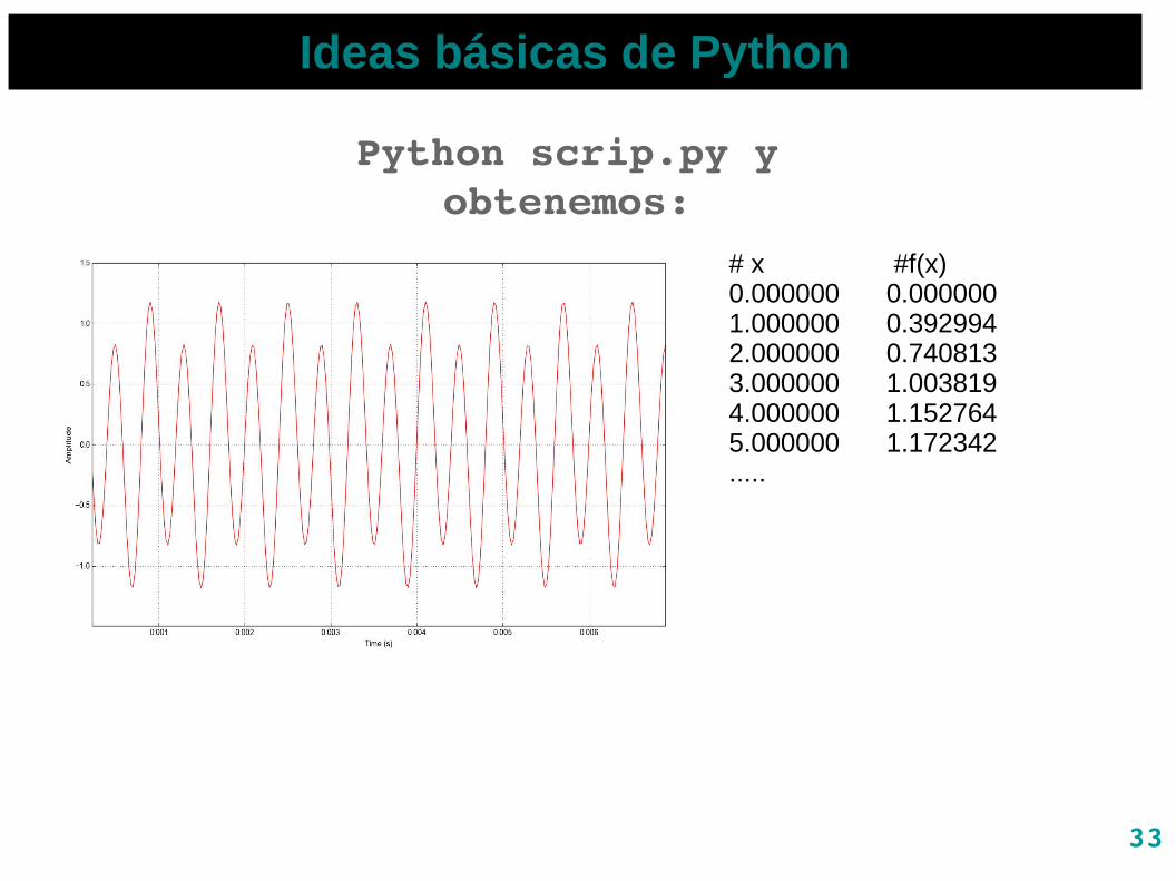
Python scrip.py y obtenemos:

# x #f(x)0.000000 0.0000001.000000 0.3929942.000000 0.7408133.000000 1.0038194.000000 1.1527645.000000 1.172342.....

34

Ideas básicas de Python

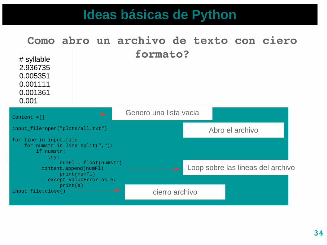
Como abro un archivo de texto con ciero formato?

Content =[]

input_file=open("plots/all.txt")

for line in input_file: for numstr in line.split(","): if numstr: try: numFl = float(numstr)

content.append(numFl) print(numFl) except ValueError as e: print(e)input_file.close()

Genero una lista vacia

Abro el archivo

Loop sobre las lineas del archivo

cierro archivo

# syllable2.9367350.0053510.0011110.0013610.001

35

Ideas básicas de Python

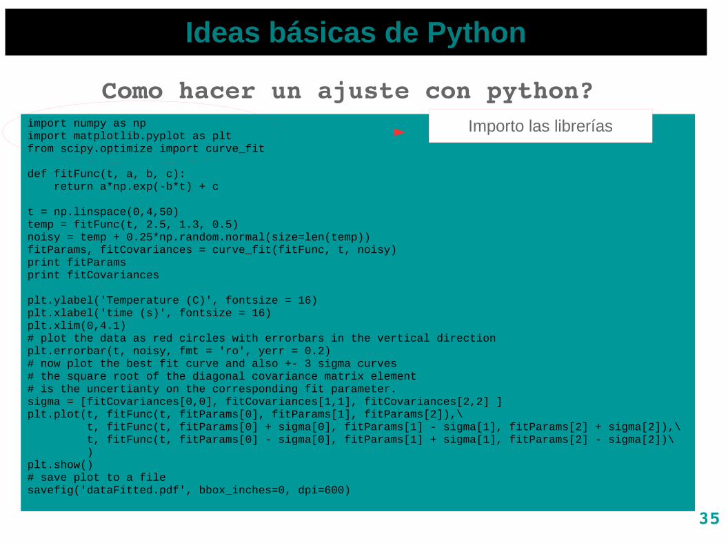
Como hacer un ajuste con python?import numpy as npimport matplotlib.pyplot as pltfrom scipy.optimize import curve_fit

def fitFunc(t, a, b, c): return a*np.exp(-b*t) + c

t = np.linspace(0,4,50)temp = fitFunc(t, 2.5, 1.3, 0.5)noisy = temp + 0.25*np.random.normal(size=len(temp))fitParams, fitCovariances = curve_fit(fitFunc, t, noisy)print fitParamsprint fitCovariances

plt.ylabel('Temperature (C)', fontsize = 16)plt.xlabel('time (s)', fontsize = 16)plt.xlim(0,4.1)# plot the data as red circles with errorbars in the vertical directionplt.errorbar(t, noisy, fmt = 'ro', yerr = 0.2)# now plot the best fit curve and also +- 3 sigma curves# the square root of the diagonal covariance matrix element # is the uncertianty on the corresponding fit parameter.sigma = [fitCovariances[0,0], fitCovariances[1,1], fitCovariances[2,2] ]plt.plot(t, fitFunc(t, fitParams[0], fitParams[1], fitParams[2]),\ t, fitFunc(t, fitParams[0] + sigma[0], fitParams[1] - sigma[1], fitParams[2] + sigma[2]),\ t, fitFunc(t, fitParams[0] - sigma[0], fitParams[1] + sigma[1], fitParams[2] - sigma[2])\ )plt.show()# save plot to a filesavefig('dataFitted.pdf', bbox_inches=0, dpi=600)

Importo las librerías

36

Ideas básicas de Python

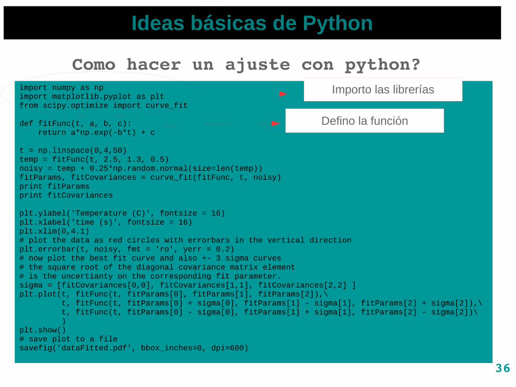
Como hacer un ajuste con python?import numpy as npimport matplotlib.pyplot as pltfrom scipy.optimize import curve_fit

def fitFunc(t, a, b, c): return a*np.exp(-b*t) + c

t = np.linspace(0,4,50)temp = fitFunc(t, 2.5, 1.3, 0.5)noisy = temp + 0.25*np.random.normal(size=len(temp))fitParams, fitCovariances = curve_fit(fitFunc, t, noisy)print fitParamsprint fitCovariances

plt.ylabel('Temperature (C)', fontsize = 16)plt.xlabel('time (s)', fontsize = 16)plt.xlim(0,4.1)# plot the data as red circles with errorbars in the vertical directionplt.errorbar(t, noisy, fmt = 'ro', yerr = 0.2)# now plot the best fit curve and also +- 3 sigma curves# the square root of the diagonal covariance matrix element # is the uncertianty on the corresponding fit parameter.sigma = [fitCovariances[0,0], fitCovariances[1,1], fitCovariances[2,2] ]plt.plot(t, fitFunc(t, fitParams[0], fitParams[1], fitParams[2]),\ t, fitFunc(t, fitParams[0] + sigma[0], fitParams[1] - sigma[1], fitParams[2] + sigma[2]),\ t, fitFunc(t, fitParams[0] - sigma[0], fitParams[1] + sigma[1], fitParams[2] - sigma[2])\ )plt.show()# save plot to a filesavefig('dataFitted.pdf', bbox_inches=0, dpi=600)

Importo las librerías

Defino la función

37

Ideas básicas de Python

Como hacer un ajuste con python?import numpy as npimport matplotlib.pyplot as pltfrom scipy.optimize import curve_fit

def fitFunc(t, a, b, c): return a*np.exp(-b*t) + c

t = np.linspace(0,4,50)temp = fitFunc(t, 2.5, 1.3, 0.5)noisy = temp + 0.25*np.random.normal(size=len(temp))fitParams, fitCovariances = curve_fit(fitFunc, t, noisy)print fitParamsprint fitCovariances

plt.ylabel('Temperature (C)', fontsize = 16)plt.xlabel('time (s)', fontsize = 16)plt.xlim(0,4.1)# plot the data as red circles with errorbars in the vertical directionplt.errorbar(t, noisy, fmt = 'ro', yerr = 0.2)# now plot the best fit curve and also +- 3 sigma curves# the square root of the diagonal covariance matrix element # is the uncertianty on the corresponding fit parameter.sigma = [fitCovariances[0,0], fitCovariances[1,1], fitCovariances[2,2] ]plt.plot(t, fitFunc(t, fitParams[0], fitParams[1], fitParams[2]),\ t, fitFunc(t, fitParams[0] + sigma[0], fitParams[1] - sigma[1], fitParams[2] + sigma[2]),\ t, fitFunc(t, fitParams[0] - sigma[0], fitParams[1] + sigma[1], fitParams[2] - sigma[2])\ )plt.show()# save plot to a filesavefig('dataFitted.pdf', bbox_inches=0, dpi=600)

Importo las librerías

Defino la función

Genero un set d datos

38

Ideas básicas de Python

Como hacer un ajuste con python?import numpy as npimport matplotlib.pyplot as pltfrom scipy.optimize import curve_fit

def fitFunc(t, a, b, c): return a*np.exp(-b*t) + c

t = np.linspace(0,4,50)temp = fitFunc(t, 2.5, 1.3, 0.5)noisy = temp + 0.25*np.random.normal(size=len(temp))fitParams, fitCovariances = curve_fit(fitFunc, t, noisy)print fitParamsprint fitCovariances

plt.ylabel('Temperature (C)', fontsize = 16)plt.xlabel('time (s)', fontsize = 16)plt.xlim(0,4.1)# plot the data as red circles with errorbars in the vertical directionplt.errorbar(t, noisy, fmt = 'ro', yerr = 0.2)# now plot the best fit curve and also +- 3 sigma curves# the square root of the diagonal covariance matrix element # is the uncertianty on the corresponding fit parameter.sigma = [fitCovariances[0,0], fitCovariances[1,1], fitCovariances[2,2] ]plt.plot(t, fitFunc(t, fitParams[0], fitParams[1], fitParams[2]),\ t, fitFunc(t, fitParams[0] + sigma[0], fitParams[1] - sigma[1], fitParams[2] + sigma[2]),\ t, fitFunc(t, fitParams[0] - sigma[0], fitParams[1] + sigma[1], fitParams[2] - sigma[2])\ )plt.show()# save plot to a filesavefig('dataFitted.pdf', bbox_inches=0, dpi=600)

Importo las librerías

Defino la función

Genero un set d datos

Importo las librerías

39

Ideas básicas de Python

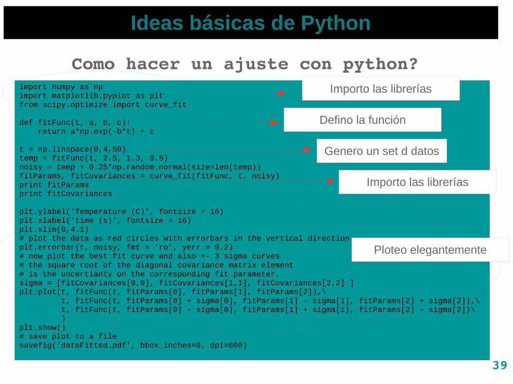
Como hacer un ajuste con python?import numpy as npimport matplotlib.pyplot as pltfrom scipy.optimize import curve_fit

def fitFunc(t, a, b, c): return a*np.exp(-b*t) + c

t = np.linspace(0,4,50)temp = fitFunc(t, 2.5, 1.3, 0.5)noisy = temp + 0.25*np.random.normal(size=len(temp))fitParams, fitCovariances = curve_fit(fitFunc, t, noisy)print fitParamsprint fitCovariances

plt.ylabel('Temperature (C)', fontsize = 16)plt.xlabel('time (s)', fontsize = 16)plt.xlim(0,4.1)# plot the data as red circles with errorbars in the vertical directionplt.errorbar(t, noisy, fmt = 'ro', yerr = 0.2)# now plot the best fit curve and also +- 3 sigma curves# the square root of the diagonal covariance matrix element # is the uncertianty on the corresponding fit parameter.sigma = [fitCovariances[0,0], fitCovariances[1,1], fitCovariances[2,2] ]plt.plot(t, fitFunc(t, fitParams[0], fitParams[1], fitParams[2]),\ t, fitFunc(t, fitParams[0] + sigma[0], fitParams[1] - sigma[1], fitParams[2] + sigma[2]),\ t, fitFunc(t, fitParams[0] - sigma[0], fitParams[1] + sigma[1], fitParams[2] - sigma[2])\ )plt.show()# save plot to a filesavefig('dataFitted.pdf', bbox_inches=0, dpi=600)

Importo las librerías

Defino la función

Genero un set d datos

Importo las librerías

Ploteo elegantemente

40

Ideas básicas de Python

Como hacer un ajuste con python?import numpy as npimport matplotlib.pyplot as pltfrom scipy.optimize import curve_fit

def fitFunc(t, a, b, c): return a*np.exp(-b*t) + c

t = np.linspace(0,4,50)temp = fitFunc(t, 2.5, 1.3, 0.5)noisy = temp + 0.25*np.random.normal(size=len(temp))fitParams, fitCovariances = curve_fit(fitFunc, t, noisy)print fitParamsprint fitCovariances

plt.ylabel('Temperature (C)', fontsize = 16)plt.xlabel('time (s)', fontsize = 16)plt.xlim(0,4.1)# plot the data as red circles with errorbars in the vertical directionplt.errorbar(t, noisy, fmt = 'ro', yerr = 0.2)# now plot the best fit curve and also +- 3 sigma curves# the square root of the diagonal covariance matrix element # is the uncertianty on the corresponding fit parameter.sigma = [fitCovariances[0,0], fitCovariances[1,1], fitCovariances[2,2] ]plt.plot(t, fitFunc(t, fitParams[0], fitParams[1], fitParams[2]),\ t, fitFunc(t, fitParams[0] + sigma[0], fitParams[1] - sigma[1], fitParams[2] + sigma[2]),\ t, fitFunc(t, fitParams[0] - sigma[0], fitParams[1] + sigma[1], fitParams[2] - sigma[2])\ )plt.show()# save plot to a filesavefig('dataFitted.pdf', bbox_inches=0, dpi=600)

Importo las librerías

Defino la función

Genero un set d datos

Importo las librerías

Salvo mi plot

Ploteo elegantemente

41

Ideas básicas de Python

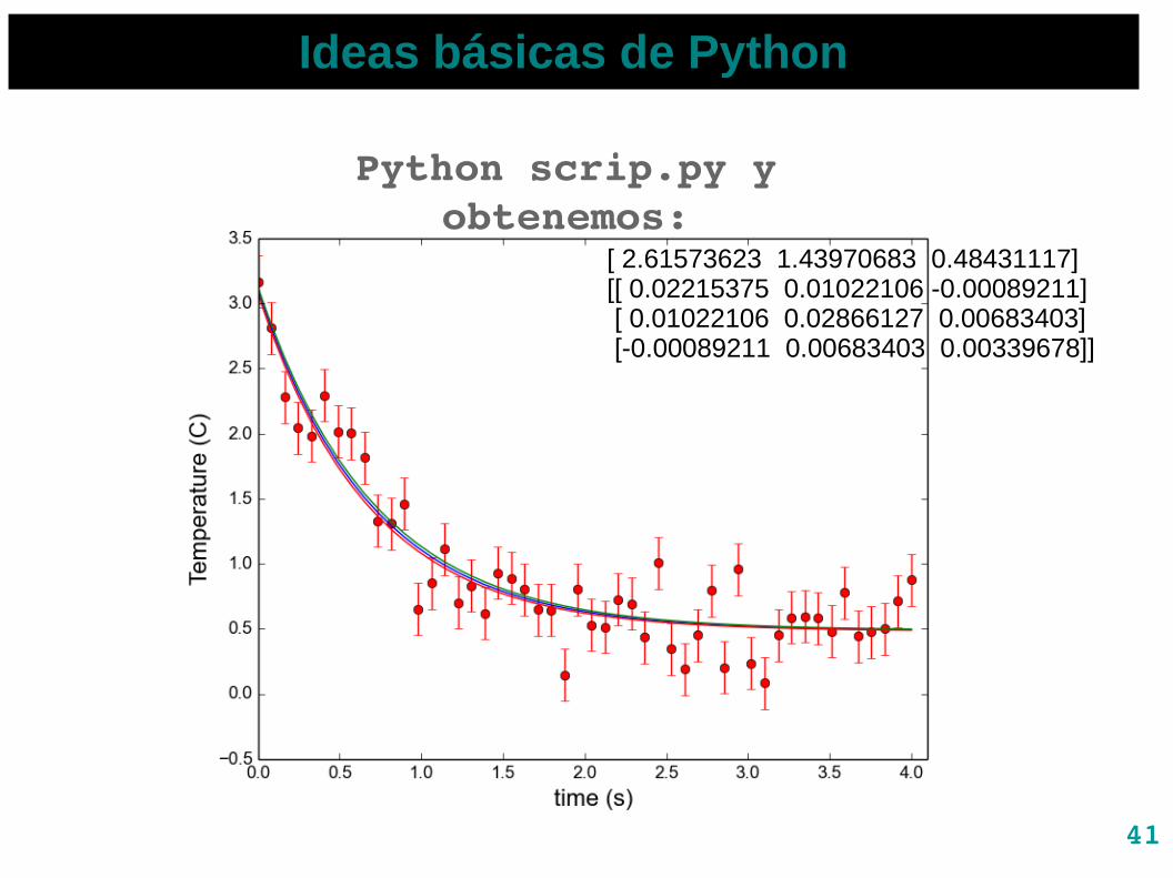
[ 2.61573623 1.43970683 0.48431117][[ 0.02215375 0.01022106 -0.00089211] [ 0.01022106 0.02866127 0.00683403] [-0.00089211 0.00683403 0.00339678]]

Python scrip.py y obtenemos:

42

Ideas básicas de Python

Para cerrar les dejo un bello ejemplo donde combino el uso de scipy, numpy y matplotlib: 

43

Ideas básicas de Python

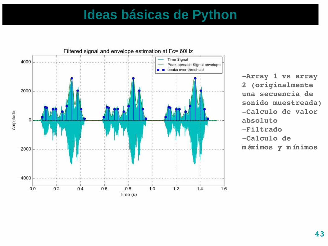
­Array 1 vs array 2 (originalmente una secuencia de sonido muestreada)­Calculo de valor absoluto­Filtrado­Calculo de máximos y mínimos

44

Ideas básicas de Python

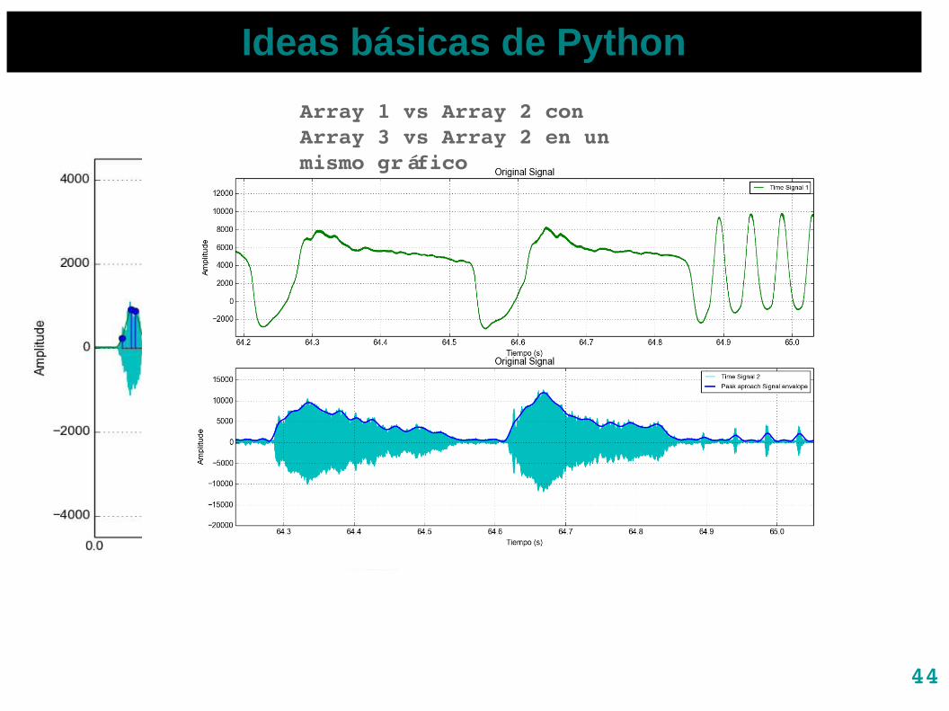
Array 1 vs Array 2 con Array 3 vs Array 2 en un mismo gráfico

45

Ideas básicas de Python

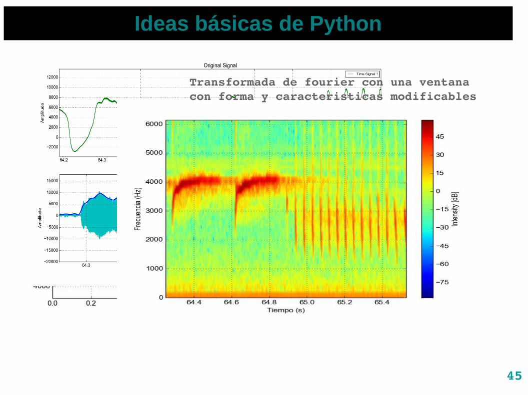
Transformada de fourier con una ventana con forma y caracteristicas modificables

46

Ideas básicas de Python

Conclusiones:

­Les dejamos una colección infinitamente grande de herramientas y recursos recombinables y reutilizables para poner en práctica.

­El salto es mas pequeño de lo que parece.

­Posibilidades de reutilizar y adaptar código a nuestras necesidades para crear soluciones prácticas.

47

Ideas básicas de Python

Backup:

https://google.github.io/styleguide/pyguide.html