water

Article

Clustering Groundwater Level Time Series of theExploited Almonte-Marismas Aquifer inSouthwest Spain

Nuria Naranjo-Fernández 1 , Carolina Guardiola-Albert 2,* , Héctor Aguilera 2 ,Carmen Serrano-Hidalgo 2 and Esperanza Montero-González 1

1 Facultad de Ciencias Geológicas, Universidad Complutense de Madrid, Calle José Antonio Novais 12,28040 Madrid, Spain; nuria.naranjo.phd@gmail.com (N.N.-F.); emontero@ucm.es (E.M.-G.)

2 Instituto Geológico y Minero de España, Calle Ríos Rosas 23, 28003 Madrid, Spain;h.aguilera@igme.es (H.A.); c.serrano@igme.es (C.S.-H.)

* Correspondence: c.guardiola@igme.es; Tel.: +34-913-495-829

Received: 3 March 2020; Accepted: 4 April 2020; Published: 8 April 2020�����������������

Abstract: Groundwater resources are regularly the principal water supply in semiarid and aridclimate areas. However, groundwater levels (GWL) in semiarid aquifers are suffering a generaldecrease because of anthropic exploitation of aquifers and the repercussions of climate change.Effective groundwater management strategies require a deep characterization of GWL fluctuations,in order to identify individual behaviors and triggering factors. In September 2019, the GuadalquivirRiver Basin Authority (CHG) declared that there was over-exploitation in three of the five groundwaterbodies of the Almonte-Marismas aquifer, Southwest Spain. For that reason, it is critical to understandGWL dynamics in this aquifer before the new Spanish Water Resources Management Plans (2021–2027)are developed. The application of GWL series clustering in hydrogeology has grown over the past fewyears, as it is an extraordinary tool that promptly provides a GWL classification; each group can berelated to different responses of a complex aquifer under any external change. In this work, GWL timeseries from 160 piezometers were analyzed for the period 1975 to 2016 and, after data pre-processing,24 piezometers were selected for clustering with k-means (static) and time series (dynamic) clusteringtechniques. Six and seven groups (k) were chosen to apply k-means. Six characterized typesof hydrodynamic behaviors were obtained with time series clustering (TSC). Number of clusterswere related to diverse affections of water exploitation depending on soil uses and hydrogeologicalspatial distribution parameters. TSC enabled us to distinguish local areas with high hydrodynamicdisturbance and to highlight a quantitative drop of GWL during the studied period.

Keywords: groundwater level hydrographs; k-means clustering; time series clustering;water resource management

1. Introduction

The increase of groundwater exploitation for intensive agricultural irrigation contributes totransformations in the natural hydrodynamics of a given area. Several studies have shown strongchanges in natural groundwater flow in over-exploited areas [1–3]. Climate change drives increasingmodifications in groundwater uses. In many cases, the decrease of groundwater levels (GWL) involvesecological degradation, especially in wetland areas [4,5]. Effective groundwater management strategiesrequire a deep characterization of GWL fluctuations, in order to identify individual behaviors andtriggering factors.

Doñana Natural Space, located in the southwest of Spain, is one of the largest protected wetlandsin Europe [6]. The study of historical piezometric databases could be a particularly challenging work

Water 2020, 12, 1063; doi:10.3390/w12041063 www.mdpi.com/journal/water

Water 2020, 12, 1063 2 of 20

in the Doñana wetland area because of heterogeneity in the records and a high number of missingvalues. While data were formerly obtained manually, piezometers have recently evolved to be partof an automated system, continuously recording GWL fluctuations. This means that the size of thedataset has increased, making the management and interpretation of the GWL data an important issue.

Clustering has frequently been applied in hydrology, e.g., in hydrochemistry studies to distinguishhydrochemical groups of water [7]. Besides this, it has been used to classify GWL hydrographs [8],to study the changes in GWL produced after an earthquake in Japan [9] and to evaluate subsurfaceflow patterns [10]. Recently clustering was also used to study hydrochemical impacts on groundwaterby altering the interaction between groundwater and surface water [11] and to evaluate the missingdata of monitoring wells [12].

There are many clustering techniques but k-means is one of the most popular, unsupervisedalgorithms applied in the geosciences and, also, in hydrogeology [13]. The aim of k-means is to dividen observations into k groups. It is relatively simple to implement, scales to log database and guaranteesconvergence [14]. Nevertheless, the number of clusters, k, has to be pre-defined and the method isvery sensitive to outliers. In addition, k-means does not consider the temporal correlation structure ofthe time series, which is an important limitation to detect changes in temporal patterns in differentgroups. To solve this limitation and handle dynamic data, time series clustering (TSC) techniques havebeen developed, modifying the similarity definition of the data or the prototype extraction function toan appropriate one [15].

In September 2019, the Guadalquivir Basin Authority (CHG in Spanish acronym) activatedthe administrative process to declare three of the five groundwater bodies that comprise theAlmonte-Marismas aquifer to be at risk of not reaching a good quantitative state. For that reason,it is critical to understand GWL dynamics in this aquifer before the new Spanish Water ResourcesManagement Plans (2021–2027) can be developed. Qualitative studies of the historical GWL datain the Almonte-Marismas aquifer exist [16–18] but they examined the data by visual inspection andnone of them give a clear categorization of GWL behavior. In general, to analyze the characteristicsand summarize the patterns of the complex fluctuation of GWL, it is important to rely on objectiveclassifications [19].

The consequences of climate change, such as increasing evaporation or more extremehydrological events (e.g., droughts), aggravate the anthropic pressure, posing a serious threat tothe Almonte-Marismas aquifer’s hydrogeological state [20]. The over-exploitation of the area isattributed to uncontrolled, unsustainable and, in many cases, illegal growth of intensively irrigatedagriculture over recent decades [21]. Unregulated and illegal pumping must be taken into accountin groundwater management evaluations [22]. When long GWL time series are available, one wayto evaluate the agricultural expansion effect on the aquifer dynamics is a deep study of the GWL byusing clustering tools.

In the present work, the aim is to apply clustering methodologies to improve the understandingof the Almonte-Marismas aquifer dynamics and obtain information that will be useful to developsustainable groundwater resource management plans. For that purpose, monthly GWL from 1975 to2016 were clustered using three different methods: visual observation (as a reference for a qualitativeanalysis), k-means [23] and TSC [15]. To the best of the authors’ knowledge, this is the first time thatTSC has been applied to a medium size GWL database with a 41 year time series.

2. Materials and Methods

2.1. Study Site

The Almonte-Marismas aquifer, in Southwest Spain, is located at the margins of the mouth ofthe Guadalquivir River (Figure 1a). This aquifer hosts the Doñana marshlands, which was floodedby groundwater and surface water and declared to be RAMSAR wetlands in 1982 [24]. At the same

Water 2020, 12, 1063 3 of 20

time, Doñana water supports the socio-economic activities developed on the area, such as agriculture,industry, mining and tourism.

Water 2020, 11, x FOR PEER REVIEW 14 of 21

time, Doñana water supports the socio-economic activities developed on the area, such as agriculture, industry, mining and tourism.

Figure 1. (a) Location and geological map; (b) Cross sections of Almonte-Marismas aquifer (Guadalquivir River Basin, GRB); and (c) Piezometers and Almonte-Acebuche rain gauge locations and piezometric surface at the end of 1997, taken from Guardiola-Albert et al. [25]. DEM: Digital Elevation Model.

Figure 1. (a) Location and geological map; (b) Cross sections of Almonte-Marismas aquifer(Guadalquivir River Basin, GRB); and (c) Piezometers and Almonte-Acebuche rain gaugelocations and piezometric surface at the end of 1997, taken from Guardiola-Albert et al. [25].DEM: Digital Elevation Model.

Water 2020, 12, 1063 4 of 20

The topography of the region falls from approximately 150 m above sea level (masl) in thenorth, to less than 1 masl in the marshland area on the coast to the south. In geological terms, it iscomposed of a complex sedimentary system of sand and gravels with some clay lenses, basal sands,silts and aeolian sands [26,27] (Figure 1a,b). The average precipitation between 1975 and 2016 wasapproximately 550 mm/year and the average annual temperature was 25 ◦C. The maximum dailyprecipitation was registered at 168.2 mm in November 2001. From June to September the maximumtemperature was 45 ◦C and the minimum temperature in winter months was 6 ◦C. The sub-humidMediterranean climate with an Atlantic influence results in high seasonality [24]. The main rechargesources are rainfall, irrigation return flow and lateral inflow from the northeast. The average rechargeis 200 hm3/year, primarily during spring and autumn [24]. The main groundwater flow runs fromnorthwest to southeast, recharging mainly from the northern and southwestern areas and discharginginto the Atlantic Ocean onto the marshland, rivers and streams that flow from the higher regions in thenorth (Figure 1c). There is no control over how much water is withdrawn for agriculture but thereare estimated increases in groundwater abstraction for irrigation, from 11 hm3/year at the beginningof the 1970s to 80 hm3/year in the mid-1990s, continuing to increase up to more than 130 hm3/year,currently [28].

The Almonte-Marismas aquifer’s complex sedimentary origins, ecological richness andgroundwater over-exploitation are three challenging factors for groundwater resource managementdecisions [27,29]. The combined effect of agricultural activities, industry and tourism have added toclimate change and led to a general decrease of GWL, changing the hydrodynamics in the area [22].As a result, several groundwater-dependent temporal ponds have disappeared [30].

2.2. Data Collection and Pre-Treatment

Groundwater monitoring has historically been carried out in the Almonte-Marismas aquifer since1903. Unfortunately, this GWL series does not retain continuity. Piezometers were first installedin 1970 [24], making it possible to have an entire database with 160 points (blue dots in Figure 1c)with different degrees of temporal continuity. Data from these piezometers (with less than 80%missing values (MV)), have been collected by the Spanish Geological Survey (IGME) and the CHGand have been used in the present work (yellow dots in Figure 1c). The period of time chosen,from October 1975 to September 2016, follows a hydrological year and registers the most data recorded.Agricultural activity grew considerably in the mid-1990s. Consequently, in order to analyze theevolution of the aquifer dynamics due to anthropic actions, the study period was subdivided intotwo sub-periods of twenty and twenty-one hydrological years: (1) October 1975–September 1995 and(2) October 1995–September 2016.

The measurements, as an absolute elevation above or under sea level, have been homogenized to amonthly time step, taking the average of all data recorded within each month. In addition, outliers andduplicates were discarded.

To study GWL responses to precipitation, rainfall data were taken from the Almonte-Acebucherain gauge (Figure 1c), which is maintained by the AEMET (Spanish State Meteorological Agency).Cumulative deviation from the mean monthly rainfall (CDR) was calculated to represent precipitationvariations in both sub-periods.

Figure 2 shows the whole approach that was followed in this study. To define a starting point(and before applying more advanced statistical techniques), visual classification of the piezometric timeseries was performed. This exercise is essential to developing a global understanding of the time series.

Water 2020, 12, 1063 5 of 20Water 2020, 11, x FOR PEER REVIEW 14 of 21

Figure 2. Flowchart of the methodological approach used in the current study. S: standardization as pre-treatment.

MV in the GWL time series have been infilled using all the available information (160 piezometers) and the missForest algorithm [31]. MissForest is a non-parametric, iterative imputation method, based on the random forest algorithm [32]. The advantage of missForest is that it does not make any assumptions about the distribution of data or imputation models [33]. It uses an iterative imputation scheme by training a random forest on the observed values of each variable in a first step. Then, it predicts the missing values and proceeds iteratively until the stopping criterion is met or the user-specified maximum number of iterations is reached. The algorithm continuously updates the imputed matrix variables, assessing its performance between iterations. This assessment is done by considering the difference between the previous and the new imputation results. As soon as this difference increases for the first time, the algorithm stops and keeps the last imputation matrix. The Normalized Root Mean Square Error (NRMSE; Equation (1)) has been obtained to evaluate the performance of the method:

NRMSE = 𝑚𝑒𝑎𝑛 (𝑋 − 𝑋 )𝑣𝑎𝑟(𝑋 ) (1)

where 𝑋 is the complete data matrix, 𝑋 is the imputed data matrix, 𝑚𝑒𝑎𝑛 and 𝑣𝑎𝑟 are, respectively, the short notation for the empirical mean and variance computed over the continuous missing values only. Good performance leads to a value of NRMSE close to 0 and bad performance results in a value approaching 1.

To perform a consistent GWL clustering it was decided to only use piezometers with a low percentage of MV in both study sub-periods (i.e., October 1975–September 1995 and October 1995–September 2016). The average MV percentage for the entire study period was T = 51.5%. For the first and second sub-periods the average MV percentages were P1 = 64.1% and P2 = 39.5%, respectively. That is the reason why a more restrictive MV threshold was applied in order to select which piezometers were used in the cluster analysis in the first sub-period, compared to the second one. The following expressions (relating P1 and P2 to T (Equations (2) and (3))) were used to decide which

Figure 2. Flowchart of the methodological approach used in the current study. S: standardizationas pre-treatment.

MV in the GWL time series have been infilled using all the available information (160 piezometers)and the missForest algorithm [31]. MissForest is a non-parametric, iterative imputation method,based on the random forest algorithm [32]. The advantage of missForest is that it does not make anyassumptions about the distribution of data or imputation models [33]. It uses an iterative imputationscheme by training a random forest on the observed values of each variable in a first step. Then,it predicts the missing values and proceeds iteratively until the stopping criterion is met or theuser-specified maximum number of iterations is reached. The algorithm continuously updates theimputed matrix variables, assessing its performance between iterations. This assessment is doneby considering the difference between the previous and the new imputation results. As soon asthis difference increases for the first time, the algorithm stops and keeps the last imputation matrix.The Normalized Root Mean Square Error (NRMSE; Equation (1)) has been obtained to evaluate theperformance of the method:

NRMSE =

√√√mean

(Xtrue −Ximp

)2

var(Xtrue)(1)

where Xtrue is the complete data matrix, Ximp is the imputed data matrix, mean and var are, respectively,the short notation for the empirical mean and variance computed over the continuous missing valuesonly. Good performance leads to a value of NRMSE close to 0 and bad performance results in a valueapproaching 1.

To perform a consistent GWL clustering it was decided to only use piezometers with a lowpercentage of MV in both study sub-periods (i.e., October 1975–September 1995 and October1995–September 2016). The average MV percentage for the entire study period was T = 51.5%.For the first and second sub-periods the average MV percentages were P1 = 64.1% and P2 = 39.5%,respectively. That is the reason why a more restrictive MV threshold was applied in order to selectwhich piezometers were used in the cluster analysis in the first sub-period, compared to the secondone. The following expressions (relating P1 and P2 to T (Equations (2) and (3))) were used to decide

Water 2020, 12, 1063 6 of 20

which MV thresholds define what piezometers from the 160 available data points remained for thecluster analysis:

MV1 = P1(2− r1) (2)

MV2 = P2(1 + r2) (3)

where r1 = P1/T and r2 = P2/T.Substituting P1, P2, r1 and r2 for their corresponding values in the equations yields an MV1

threshold of 48.4% for the first sub-period and an MV2 threshold of 69.8% for the second sub-period.Rounding up these figures, the piezometers that have less than 50% MV for the first sub-period and70% MV for the second sub-period have been kept, resulting in 24 piezometers in total (yellow dots inFigure 1c). The general statistics for these 24 piezometers can be seen in Appendix A, Table A1.

To avoid the scaling effects of GWL values while clustering, the imputed monthly piezometricseries were standardized. This step was carried out before visual and k-means clustering and it isalready implemented in the algorithm used to perform TSC.

2.3. K-Means Clustering

K-means clustering is one of most common methods for exploratory data analysis. This techniquecan identify groups in the dataset that show similar patterns or equal trends. Specifically, k-meansdivides up the data into pre-defined, non-overlapping groups, where every data point belongs to onlyone group or cluster. First of all, the random partition method randomly assigns a cluster to eachobservation and then the algorithm proceeds to the update step, computing the initial mean to be thecentroid of the cluster’s randomly assigned points.

The standard algorithm of k-means [34] (Equation (4)), minimizes the sum of squares of thedistance between data points within a cluster and the centroid of that cluster:

W(CK) =∑

Xi ∈ Ck

(xi − µk)2 (4)

In the present case study, xi is the data vector with monthly measurements corresponding topiezometer i, Xi is the set of piezometers that belongs to cluster CK and µk is the centroid, computed asthe mean value of the data vector belonging to cluster CK. Each data vector (xi) is assigned to a clusterwhen its distance to the centroid, W(CK), is at a minimum.

The appropriate number of clusters is given by the point where the sedimentation graph changesthe trend, drawing an “elbow” [35]. The sedimentation graph plots a clustering score as a function ofthe number of clusters and the elbow method is a heuristic method for interpreting and validatingconsistency. The score is generally a measure of the input data on the k-means objective function(e.g., sum of W(CK) across clusters). The k-means algorithm was run with the R package factoextra [36].

2.4. Time Series Clustering (TSC)

The TSC method considers time series distribution. As with the k-means method, it has a stochasticnature due to its random start. TSC was run with the R package dtwclust [15].

In order to classify all piezometers, partitional clustering [37] was selected to create partitions.The specification of the number of clusters (k) is tedious work that must be performed before startingthe algorithm. The optimal k was identified by using internal clustering validity indices (CVIs).Cluster validity is a set of techniques that have been developed to find the best k without any previousclass information. Based on similar works [38,39], three internal CVI indexes were used to choosek: Dunn (D), Davies–Bouldin (DB) and Calinski–Harabasz (CH). D is a ratio-type index and itscohesion is calculated by the distance to its nearest neighbor and the separation by the maximumcluster diameter [40]. DB is one of the most popular indices and it was based on the distance between

Water 2020, 12, 1063 7 of 20

centroids [41]. CH cohesion is estimated based on the distance from the points in a cluster to itscentroid [42].

Depending on the distance of the disturbance and the aquifer characteristics, GWL responsescan be registered with a lag of days or months from one location to another. Considering thissingularity of GWL behavior, the most appropriate distance to measure GWL time series is Shape-BasedDistance (SBD) [15]. SBD warps the time series and it is based on the cross-correlation with coefficientnormalization (NCCc) and shape extraction as a prototype function (Equation (5)) [37]:

SBD(x, y) = 1−max(NCCc(x, y))‖x‖2‖y‖2

(5)

where ‖ ‖2 denotes the standard L2 norm of the series and SBD(x, y) values range between 0(perfect similarity) and 2 (unequal time series).

3. Results and Discussion

3.1. Imputation Piezometry and Visual Classification

Monthly imputation of the 41-year time series for the 24 piezometers with the missForest algorithmresulted in an NRMSE of 0.05, indicating a good performance of the imputation scheme. This smallerror can mainly be explained by the lack of uneven piezometer variations at a monthly scale, which ispresent in other kinds of time series (e.g., temperature), and by the high number of piezometersavailable for imputation.

Table 1 shows how many piezometers integrate every cluster for each sub-period. Figure 3represents the spatial distribution of the different clusters obtained. Visual classification results forboth study sub-periods are shown in the first row of Figure 3a,b and in Figures 4 and 5. A layercorresponding to a rough spatial distribution of the groundwater extractions in the two differentsub-periods [25,43] is also included in Figure 3 (in grey). To ease the interpretation, the raw piezometrictime evolution for each visual cluster is shown in Figure 4 (clusters named V1.1, V1.2, V1.3 and V1.4 forthe first sub-period) and Figure 5 (clusters named V2.1, V2.2, V2.3 and V2.4 for the second sub-period).Piezometric time series are plotted in the primary Y axis with grey lines; the mean of each GWL clusteris shown in the secondary Y axis, with colored lines.

It is difficult to compare our GWL classes (Figures 3 and 4) with the ones obtained from the 15 yearseries through visual inspection by UPC [16] and, in addition, those published in Manzano et al. [44].These authors only showed GWL evolution at seven points within the same study area but withouttrying to find analogous piezometric evolution at different points.

Table 1. Number of piezometers in each obtained cluster. Sub-period 1: from October 1975 to September1995. Sub-period 2: from October 1995 to September 2016.

Method Sub-Period Cluster 1 Cluster 2 Cluster 3 Cluster 4 Cluster 5 Cluster 6 Cluster 7

Visual1 10 4 7 3 - - -

2 10 5 6 3 - - -

k-means1 1 2 5 1 3 12 -

2 1 8 4 1 5 1 4

TSC1 3 2 2 3 4 6 4

2 1 6 4 2 2 7 2

Water 2020, 12, 1063 8 of 20

Visual analysis found four different groups for both sub-periods. All visual cluster groups have adifferent spatial distribution when comparing the first and second sub-periods studied (Figure 3a,b).The main difference between the two sub-periods is that the clustering spatial distribution is moreirregular in the second one. This could be attributed to an increase in the number of pumping wells(grey zones in Figure 3), in addition to climate change effects that could reduce the recharge rate [45].Water 2020, 11, x FOR PEER REVIEW 14 of 21

Figure 3. Spatial distribution of piezometer groups for the three clustering methods applied. An approximate distribution of the pumping wells [25,43] is shown in grey. (a) Visual clustering for first sub-period (October 1975 to September 1995); (b) Visual clustering for second sub-period (October 1995 to September 2016); (c) k-means clustering for first sub-period; (d) k-means clustering for second sub-period; (e) Time series clustering (TSC) for first sub-period; (f) TSC for second sub-period.

Figure 3. Spatial distribution of piezometer groups for the three clustering methods applied.An approximate distribution of the pumping wells [25,43] is shown in grey. (a) Visual clustering for firstsub-period (October 1975 to September 1995); (b) Visual clustering for second sub-period (October 1995to September 2016); (c) k-means clustering for first sub-period; (d) k-means clustering for secondsub-period; (e) Time series clustering (TSC) for first sub-period; (f) TSC for second sub-period.

Water 2020, 12, 1063 9 of 20Water 2020, 11, x FOR PEER REVIEW 14 of 21

Figure 4. Groundwater levels (GWL) series (grey lines), mean of the GWL cluster series (colored lines) from October 1975 to September 1995 by visual clustering and cumulative deviation from the mean monthly rainfall (CDR).

Figure 5. GWL series (grey lines), mean of the GWL cluster series (colored lines) from October 1995 to September 2016 by visual clustering and cumulative deviation from the mean monthly rainfall (CDR).

It is difficult to compare our GWL classes (Figures 3 and 4) with the ones obtained from the 15 year series through visual inspection by UPC [16] and, in addition, those published in Manzano et al. [44]. These authors only showed GWL evolution at seven points within the same study area but without trying to find analogous piezometric evolution at different points.

Visual analysis found four different groups for both sub-periods. All visual cluster groups have a different spatial distribution when comparing the first and second sub-periods studied (Figures 3a and 3b). The main difference between the two sub-periods is that the clustering spatial distribution is more irregular in the second one. This could be attributed to an increase in the number of pumping wells (grey zones in Figure 3), in addition to climate change effects that could reduce the recharge rate [45].

At the end of the first sub-period there is a generally descending trend of GWL and a maximum average local oscillation of 5 m (Figure 4). The series that comprise groups V1.2 and V1.3 have piezometers with GWL between 0 and 80 masl, while V1.1 and V1.4 have a lower range, between −10 and 30 masl. This reflects the fact that series with visually similar GWL oscillations are located in different areas of the aquifer (Figure 3a). All of the groups exhibit time variations that may be due to extractions, as well as the recharge–discharge pattern characteristics of the hydrological cycle (e.g., compared with the CDR line). Visually, it looks like V1.1 and V1.3 are highly affected by pumping due to their cyclical oscillation over a year, ranging from 2 to 6 m. Group V1.4 seems to be located in an area exploited in the first half of the sub-period, but not in the second period. Until 1990, cluster V1.2 fluctuations followed the same temporal evolution that Custodio [4] assigned to undisturbed

Figure 4. Groundwater levels (GWL) series (grey lines), mean of the GWL cluster series (colored lines)from October 1975 to September 1995 by visual clustering and cumulative deviation from the meanmonthly rainfall (CDR).

Water 2020, 11, x FOR PEER REVIEW 14 of 21

Figure 4. Groundwater levels (GWL) series (grey lines), mean of the GWL cluster series (colored lines) from October 1975 to September 1995 by visual clustering and cumulative deviation from the mean monthly rainfall (CDR).

Figure 5. GWL series (grey lines), mean of the GWL cluster series (colored lines) from October 1995 to September 2016 by visual clustering and cumulative deviation from the mean monthly rainfall (CDR).

It is difficult to compare our GWL classes (Figures 3 and 4) with the ones obtained from the 15 year series through visual inspection by UPC [16] and, in addition, those published in Manzano et al. [44]. These authors only showed GWL evolution at seven points within the same study area but without trying to find analogous piezometric evolution at different points.

Visual analysis found four different groups for both sub-periods. All visual cluster groups have a different spatial distribution when comparing the first and second sub-periods studied (Figures 3a and 3b). The main difference between the two sub-periods is that the clustering spatial distribution is more irregular in the second one. This could be attributed to an increase in the number of pumping wells (grey zones in Figure 3), in addition to climate change effects that could reduce the recharge rate [45].

At the end of the first sub-period there is a generally descending trend of GWL and a maximum average local oscillation of 5 m (Figure 4). The series that comprise groups V1.2 and V1.3 have piezometers with GWL between 0 and 80 masl, while V1.1 and V1.4 have a lower range, between −10 and 30 masl. This reflects the fact that series with visually similar GWL oscillations are located in different areas of the aquifer (Figure 3a). All of the groups exhibit time variations that may be due to extractions, as well as the recharge–discharge pattern characteristics of the hydrological cycle (e.g., compared with the CDR line). Visually, it looks like V1.1 and V1.3 are highly affected by pumping due to their cyclical oscillation over a year, ranging from 2 to 6 m. Group V1.4 seems to be located in an area exploited in the first half of the sub-period, but not in the second period. Until 1990, cluster V1.2 fluctuations followed the same temporal evolution that Custodio [4] assigned to undisturbed

Figure 5. GWL series (grey lines), mean of the GWL cluster series (colored lines) from October 1995 toSeptember 2016 by visual clustering and cumulative deviation from the mean monthly rainfall (CDR).

At the end of the first sub-period there is a generally descending trend of GWL and a maximumaverage local oscillation of 5 m (Figure 4). The series that comprise groups V1.2 and V1.3 havepiezometers with GWL between 0 and 80 masl, while V1.1 and V1.4 have a lower range, between −10and 30 masl. This reflects the fact that series with visually similar GWL oscillations are located indifferent areas of the aquifer (Figure 3a). All of the groups exhibit time variations that may be dueto extractions, as well as the recharge–discharge pattern characteristics of the hydrological cycle(e.g., compared with the CDR line). Visually, it looks like V1.1 and V1.3 are highly affected by pumpingdue to their cyclical oscillation over a year, ranging from 2 to 6 m. Group V1.4 seems to be located in anarea exploited in the first half of the sub-period, but not in the second period. Until 1990, cluster V1.2fluctuations followed the same temporal evolution that Custodio [4] assigned to undisturbed GWL.Furthermore, the reduced influence of anthropic actions is corroborated by the fact that piezometryhas the same trend as the CDR curve (Figure 4). Among the four cluster groups, V1.4 presents thehighest average level decrease of around 7 m (from 1975 to 1995). The main feature revealed by theseresults is that, between 1975 and 1995, anthropic impacts were already affecting the aquifer as GWLwas not recuperating after the pumping cycle.

For the second sub-period, Figure 5 shows that the order of the groups from highest to lowestinter-annual oscillation is V2.2, V2.1, V2.3 and V2.4. All groups have a descending trend but at varyingdegrees. The V2.4 graph (Figure 5) shows the same trend as the CDR and the smallest decrease (of up to2 m) reflects low anthropic intervention. V2.1, V2.2 and V2.3 have GWL between −10 and 40 masl andGWL in V2.4 is between 20 to 90 masl because of the altitude at the different locations. As in the first

Water 2020, 12, 1063 10 of 20

study sub-period, the wide GWL ranges are a consequence of the classification criteria (GWL behavior)and not just because of location or average values. For example, V2.4 presents a greater GWL rangebecause two piezometers (yellow dots in Figure 3b) are located at the highest topographical area andgroundwater table. V2.3 is the group with the highest drawdown in this second sub-period, up to6 m on average. Observed drawdowns are in accordance with the piezometric descent that wasestimated for the whole of the Almonte-Marismas aquifer between 1994 and 2012 (Olías-Álvarez andRodríguez-Rodríguez [17]); this ranged from 2 to 6 m. Cluster V.2.1 shows high fluctuations of upto 4 m, attributed to pumping effects. However, time variations are similar to the ones seen in CDR,which also shows the climate response. This feature could be explained by merging climate oscillationsand pumping effects seen at the locations in this cluster V2.1 (Figure 3).

Visual cluster results allow us to have an overview of the piezometer responses along eachsub-period. In addition, this approach is a qualitative baseline for evaluating and comparing theresults of the mathematical methods.

3.2. K-Means Clustering

As explained in the Section 2, when applying k-means clustering, the number of clusters k has beendefined with the aid of the sedimentation graph (Figure 6). Both sedimentation curves for first (darkblue) and second (red) study sub-periods change their trend at the point which indicates the optimalnumber of clusters (i.e., the elbow). Both curves show smoothly decreasing trends and, given that themaximum number of clusters is 24, points around the second inflexion point in each period were testedand a final value of k chosen as a trade-off between complexity and representativeness. Consequently,k = 6 and k = 7 were taken to be the optimal number of clusters to run the k-means algorithm for thefirst and the second study sub-periods, respectively (Figure 6). Initially, it can be interpreted that thek-means method distinguishes more GWL variation groups that were found by visual classification.However, two and three groups are formed by just one piezometer in each sub-period. These clusterswith a single piezometer correspond to singular time series variations that k-means cannot group.Water 2020, 11, x FOR PEER REVIEW 14 of 21

Figure 6. K-means sedimentation graphs of cluster sub-periods. Blue dots represent the first sub-period (from October 1975 to September 1995) and red dots the second sub-period (from October 1995 to September 2016).

As a visual classification, k-means has more spatial continuity in the cluster groups in the first sub-period than in the second period (Figures 3c and 3d). For both sub-periods and each k-means cluster, Figures 7 and 8 plot the raw piezometric series (grey), and the average raw series (colored).

Figure 7. GWL series (grey lines), mean of the GWL cluster series (colored line) from October 1975 to September 1995 (first sub-period), classified by k-means clustering and cumulative deviation from the mean monthly rainfall (CDR).

In the first sub-period, K1.3 is the group with the highest GWL range (Figure 7) due to the sparse spatial distribution of the piezometers. For example, there is one point located in the piezometric dome (Figure 1c), where important recharge rates take place. K1.3 is almost the same group as V1.2, with just one piezometer more and the same trend as the CDR. These groups of piezometers do not show fluctuations affected by direct pumping, but a decreasing trend can be seen since 1990. Groups

Figure 6. K-means sedimentation graphs of cluster sub-periods. Blue dots represent the first sub-period(from October 1975 to September 1995) and red dots the second sub-period (from October 1995 toSeptember 2016).

As a visual classification, k-means has more spatial continuity in the cluster groups in the firstsub-period than in the second period (Figure 3c,d). For both sub-periods and each k-means cluster,Figures 7 and 8 plot the raw piezometric series (grey), and the average raw series (colored).

Water 2020, 12, 1063 11 of 20

Water 2020, 11, x FOR PEER REVIEW 14 of 21

Figure 6. K-means sedimentation graphs of cluster sub-periods. Blue dots represent the first sub-period (from October 1975 to September 1995) and red dots the second sub-period (from October 1995 to September 2016).

As a visual classification, k-means has more spatial continuity in the cluster groups in the first sub-period than in the second period (Figures 3c and 3d). For both sub-periods and each k-means cluster, Figures 7 and 8 plot the raw piezometric series (grey), and the average raw series (colored).

Figure 7. GWL series (grey lines), mean of the GWL cluster series (colored line) from October 1975 to September 1995 (first sub-period), classified by k-means clustering and cumulative deviation from the mean monthly rainfall (CDR).

In the first sub-period, K1.3 is the group with the highest GWL range (Figure 7) due to the sparse spatial distribution of the piezometers. For example, there is one point located in the piezometric dome (Figure 1c), where important recharge rates take place. K1.3 is almost the same group as V1.2, with just one piezometer more and the same trend as the CDR. These groups of piezometers do not show fluctuations affected by direct pumping, but a decreasing trend can be seen since 1990. Groups

Figure 7. GWL series (grey lines), mean of the GWL cluster series (colored line) from October 1975 toSeptember 1995 (first sub-period), classified by k-means clustering and cumulative deviation from themean monthly rainfall (CDR).

Water 2020, 11, x FOR PEER REVIEW 14 of 21

K1.2, K1.5 and K1.6 have GWL between −10 and 30 masl and they correspond to piezometers located in the pumping areas with high anthropic changes in the natural hydrodynamics. K1.2 and K1.5 (Figure 7) have an average time series that can correspond to V1.3 (Figure 4) and K1.6 (Figure 7) corresponds to V1.1 and V1.4 (Figure 4). These groups are affected by groundwater extractions and are differently classified when using visual or k-means clustering. K1.5 and K1.6 average series show clear cycles that are attributed to the effects of groundwater extraction, as well as an important, descending trend of up to 8 m, on average (Figure 7). Spatially, they are located in an area of high agricultural development (Figure 3c). Finally, both groups K1.1 and K1.4 are composed of a single piezometer (Table 1), located in regions not affected by irrigation pumping during this first sub-period (Figure 3c).

Figure 8. GWL series (grey lines), mean of the GWL cluster series (colored line) from October 1995 to September 2016 (second sub-period), classified by k-means clustering and cumulative deviation from the mean monthly rainfall (CDR).

For the second sub-period, it was observed that the GWL variations are greater than the first sub-period (Figure 8). Groups K2.1, K2.4 and K2.6 are composed of a single piezometer (Figure 8, Table 1). K2.1 is the same piezometer as K1.1. It presents a different GWL pattern than the other piezometers (with small oscillations from October 1984) and an important drawdown at the beginning of 2009 (Figures 7 and 8). These abrupt variations suggest that there could be errors in the data acquisition from this piezometer. K2.4 temporal behavior indicates that aquifer exploitation started at the beginning of 2007 near this point and this could be the reason why the GWL behavior does not fit with other groups. The opposite behavior was seen in K2.6, with smooth variations during the second half of the sub-period. K2.3 does not show a clearly descending trend, with piezometers in very different areas of the aquifer (Figure 3d) and appearing as a smoothed signal of the CDR. The average series of K2.2, K2.5 and K2.7 have a decreasing tendency (Figure 8) due to the growing groundwater extractions in the nearby areas (Figure 3d). In particular, the K2.2 group presents the most pronounced drawdowns of up to 8 m, and mainly comprises piezometers located in central areas of the aquifer. It appears to correspond to an area that began to be exploited later than zone K2.5 but, as piezometry suggests, with a greater intensity reflected by a faster descent since the year

Figure 8. GWL series (grey lines), mean of the GWL cluster series (colored line) from October 1995 toSeptember 2016 (second sub-period), classified by k-means clustering and cumulative deviation fromthe mean monthly rainfall (CDR).

In the first sub-period, K1.3 is the group with the highest GWL range (Figure 7) due to the sparsespatial distribution of the piezometers. For example, there is one point located in the piezometric dome(Figure 1c), where important recharge rates take place. K1.3 is almost the same group as V1.2, with justone piezometer more and the same trend as the CDR. These groups of piezometers do not show

Water 2020, 12, 1063 12 of 20

fluctuations affected by direct pumping, but a decreasing trend can be seen since 1990. Groups K1.2,K1.5 and K1.6 have GWL between −10 and 30 masl and they correspond to piezometers located in thepumping areas with high anthropic changes in the natural hydrodynamics. K1.2 and K1.5 (Figure 7)have an average time series that can correspond to V1.3 (Figure 4) and K1.6 (Figure 7) corresponds toV1.1 and V1.4 (Figure 4). These groups are affected by groundwater extractions and are differentlyclassified when using visual or k-means clustering. K1.5 and K1.6 average series show clear cycles thatare attributed to the effects of groundwater extraction, as well as an important, descending trend of upto 8 m, on average (Figure 7). Spatially, they are located in an area of high agricultural development(Figure 3c). Finally, both groups K1.1 and K1.4 are composed of a single piezometer (Table 1), located inregions not affected by irrigation pumping during this first sub-period (Figure 3c).

For the second sub-period, it was observed that the GWL variations are greater than the firstsub-period (Figure 8). Groups K2.1, K2.4 and K2.6 are composed of a single piezometer (Figure 8,Table 1). K2.1 is the same piezometer as K1.1. It presents a different GWL pattern than the otherpiezometers (with small oscillations from October 1984) and an important drawdown at the beginningof 2009 (Figures 7 and 8). These abrupt variations suggest that there could be errors in the dataacquisition from this piezometer. K2.4 temporal behavior indicates that aquifer exploitation startedat the beginning of 2007 near this point and this could be the reason why the GWL behavior doesnot fit with other groups. The opposite behavior was seen in K2.6, with smooth variations duringthe second half of the sub-period. K2.3 does not show a clearly descending trend, with piezometersin very different areas of the aquifer (Figure 3d) and appearing as a smoothed signal of the CDR.The average series of K2.2, K2.5 and K2.7 have a decreasing tendency (Figure 8) due to the growinggroundwater extractions in the nearby areas (Figure 3d). In particular, the K2.2 group presents themost pronounced drawdowns of up to 8 m, and mainly comprises piezometers located in central areasof the aquifer. It appears to correspond to an area that began to be exploited later than zone K2.5but, as piezometry suggests, with a greater intensity reflected by a faster descent since the year 2000.The average oscillation patterns are more regular for clusters K2.5 and K2.7; this can be explained byirrigation and geological heterogeneity.

When we compare k-means results with visual classification however, some k-means groupsrepresent a merge of hydrogeological behavior due to exploitation for irrigation of different types of crops(e.g., berries, citrus) or other uses (e.g., drinking water supply), it could be seen in the different patternsof K2.2, K2.5 and K2.7 (Figure 8). On the other hand, groups K1.3 and K2.3 have strong similitudeswith the CDR graph. Similar k-means results were found by Boomfield et al. [8] with a 30-year monthlyGWL series. These were in a limestone and chalk aquifer located in the UK. However, they highlightthe relationship between GWL and geological characteristics for 74 points, spatially distributed across2000 km2. In the present study (and by comparing cluster spatial locations (Figure 3) with the geologicaldistribution (Figure 1a)), it was observed that GWL are not always dependent on geology. However,cluster groups are in agreement with the findings in Boomfield et al. [8], regarding the identification ofanthropogenically impacted groundwater hydrographs showing declining trends (e.g., clusters K1.6or K2.2).

3.3. Time Series Clustering

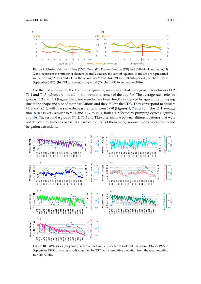
Figure 9 shows the CVI values for a different number of clusters in both sub-periods. Following thecriteria explained in Section 2, k was set to 7 in both sub-periods; D, DB and CH present an increase(marked with a red line in Figure 9). Only one of the clusters in the second sub-period had justone piezometer.

Water 2020, 12, 1063 13 of 20

Water 2020, 11, x FOR PEER REVIEW 14 of 21

2000. The average oscillation patterns are more regular for clusters K2.5 and K2.7; this can be explained by irrigation and geological heterogeneity.

When we compare k-means results with visual classification however, some k-means groups represent a merge of hydrogeological behavior due to exploitation for irrigation of different types of crops (e.g., berries, citrus) or other uses (e.g., drinking water supply), it could be seen in the different patterns of K2.2, K2.5 and K2.7 (Figure 8). On the other hand, groups K1.3 and K2.3 have strong similitudes with the CDR graph. Similar k-means results were found by Boomfield et al. [8] with a 30-year monthly GWL series. These were in a limestone and chalk aquifer located in the UK. However, they highlight the relationship between GWL and geological characteristics for 74 points, spatially distributed across 2000 km2. In the present study (and by comparing cluster spatial locations (Figure 3) with the geological distribution (Figure 1a)), it was observed that GWL are not always dependent on geology. However, cluster groups are in agreement with the findings in Boomfield et al. [8], regarding the identification of anthropogenically impacted groundwater hydrographs showing declining trends (e.g., clusters K1.6 or K2.2).

3.3. Time Series Clustering

Figure 9 shows the CVI values for a different number of clusters in both sub-periods. Following the criteria explained in Section 2, k was set to 7 in both sub-periods; D, DB and CH present an increase (marked with a red line in Figure 9). Only one of the clusters in the second sub-period had just one piezometer.

Figure 9. Cluster Validity Indices (CVI): Dunn (D), Davies–Bouldin (DB) and Calinski–Harabasz (CH). X axes represent the number of clusters (k) and Y axes are the sum-of-squares. D and DB are represented in the primary Y axis and CH in the secondary Y axis. (a) CVI for first sub-period (October 1975 to September 1995). (b) CVI for second sub-period (October 1995 to September 2016).

For the first sub-period, the TSC map (Figure 3e) reveals a spatial homogeneity for clusters T1.2, T1.4 and T1.5, which are located in the north and center of the aquifer. The average raw series of groups T1.3 and T1.4 (Figure 10) do not seem to have been directly influenced by agricultural pumping, due to the shape and size of their oscillations and they follow the CDR. They correspond to clusters V1.2 and K1.3, with the same decreasing trend from 1990 (Figures 4, 7 and 10). The T1.1 average time series is very similar to V1.1 and T1.7 to V1.4, both are affected by pumping cycles (Figures 4 and 10). The rest of the groups (T1.2, T1.5 and T1.6) discriminate between different patterns that were not detected by k-means or visual classification. All of them merge annual hydrological cycles and irrigation extractions.

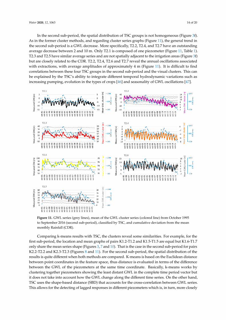
In the second sub-period, the spatial distribution of TSC groups is not homogeneous (Figure 3f). As in the former cluster methods, and regarding cluster series graphs (Figure 11), the general trend in the second sub-period is a GWL decrease. More specifically, T2.2, T2.4, and T2.7 have an outstanding average decrease between 2 and 10 m. Only T2.1 is composed of one piezometer (Figure 11, Table 1). T2.3 and T2.5 have similar average series and are not spatially adjacent to the irrigation areas (Figure 3f) but are closely related to the CDR. T2.2, T2.4, T2.6 and T2.7 reveal the annual oscillations associated with extractions, with average amplitudes of approximately 4 m (Figure 11). It is difficult to find correlations between these four TSC groups in the second sub-period and the

Figure 9. Cluster Validity Indices (CVI): Dunn (D), Davies–Bouldin (DB) and Calinski–Harabasz (CH).X axes represent the number of clusters (k) and Y axes are the sum-of-squares. D and DB are representedin the primary Y axis and CH in the secondary Y axis. (a) CVI for first sub-period (October 1975 toSeptember 1995). (b) CVI for second sub-period (October 1995 to September 2016).

For the first sub-period, the TSC map (Figure 3e) reveals a spatial homogeneity for clusters T1.2,T1.4 and T1.5, which are located in the north and center of the aquifer. The average raw series ofgroups T1.3 and T1.4 (Figure 10) do not seem to have been directly influenced by agricultural pumping,due to the shape and size of their oscillations and they follow the CDR. They correspond to clustersV1.2 and K1.3, with the same decreasing trend from 1990 (Figures 4, 7 and 10). The T1.1 averagetime series is very similar to V1.1 and T1.7 to V1.4, both are affected by pumping cycles (Figures 4and 10). The rest of the groups (T1.2, T1.5 and T1.6) discriminate between different patterns that werenot detected by k-means or visual classification. All of them merge annual hydrological cycles andirrigation extractions.

Water 2020, 11, x FOR PEER REVIEW 14 of 21

visual clusters. This can be explained by the TSC’s ability to integrate different temporal hydrodynamic variations such as increasing pumping, evolution in the types of crops [46] and seasonality of GWL oscillations [47].

Figure 10. GWL series (grey lines), mean of the GWL cluster series (colored line) from October 1975 to September 1995 (first sub-period), classified by TSC, and cumulative deviation from the mean monthly rainfall (CDR).

Figure 10. GWL series (grey lines), mean of the GWL cluster series (colored line) from October 1975 toSeptember 1995 (first sub-period), classified by TSC, and cumulative deviation from the mean monthlyrainfall (CDR).

Water 2020, 12, 1063 14 of 20

In the second sub-period, the spatial distribution of TSC groups is not homogeneous (Figure 3f).As in the former cluster methods, and regarding cluster series graphs (Figure 11), the general trend inthe second sub-period is a GWL decrease. More specifically, T2.2, T2.4, and T2.7 have an outstandingaverage decrease between 2 and 10 m. Only T2.1 is composed of one piezometer (Figure 11, Table 1).T2.3 and T2.5 have similar average series and are not spatially adjacent to the irrigation areas (Figure 3f)but are closely related to the CDR. T2.2, T2.4, T2.6 and T2.7 reveal the annual oscillations associatedwith extractions, with average amplitudes of approximately 4 m (Figure 11). It is difficult to findcorrelations between these four TSC groups in the second sub-period and the visual clusters. This canbe explained by the TSC’s ability to integrate different temporal hydrodynamic variations such asincreasing pumping, evolution in the types of crops [46] and seasonality of GWL oscillations [47].Water 2020, 11, x FOR PEER REVIEW 14 of 21

Figure 11. GWL series (grey lines), mean of the GWL cluster series (colored line) from October 1995 to September 2016 (second sub-period), classified by TSC, and cumulative deviation from the mean monthly Rainfall (CDR).

Comparing k-means results with TSC, the clusters reveal some similarities. For example, for the first sub-period, the location and mean graphs of pairs K1.2-T1.2 and K1.5-T1.5 are equal but K1.6-T1.7 only share the mean series shape (Figures 3, 7 and 10). That is the case in the second sub-period for pairs K2.2-T2.2 and K2.3-T2.3 (Figures 8 and 11). For the second sub-period, the spatial distribution of the results is quite different when both methods are compared. K-means is based on the Euclidean distance between point coordinates in the feature space, thus distance is evaluated in terms of the difference between the GWL of the piezometers at the same time coordinate. Basically, k-means works by clustering together piezometers showing the least distant GWL in the complete time period vector but it does not take into account how the GWL change along the different time series. On the other hand, TSC uses the shape-based distance (SBD) that accounts for the cross-correlation between GWL series. This allows for the detecting of lagged responses in different piezometers which is, in turn, more closely related to the hydrodynamic characteristics [48]. TSC warps the series in order to fit the oscillation curves. This is confirmed by the results, for example K1.4 is composed of only one piezometer (104140047, Appendix A, Table A1). This point is far away from the other 23 points and is located in the northern part of the aquifer with a higher topographic elevation (Figure 1c). On the other hand, the same piezometer is included with another three piezometers in the T1.4 group. The average mean of T1.4 GWL series is similar to K1.4 but smoothed out. This means that there are four points with similar patterns but k-means could not detect it (Figures 7 and 10). Furthermore, unlike most k-means clusters, that show relatively constant GWL trends (Figures 7 and 8), several TSC clusters (T1.1, T1.6, T1.7, T2.2, T2.4 and T2.7), present clearly decreasing patterns (Figures 10 and 11).

In the second sub-period, there are at least two groups with similar GWL behavior to the CDR time series. As aquifer storage is depleted because of exploitation, the rainfall dependency of the

Figure 11. GWL series (grey lines), mean of the GWL cluster series (colored line) from October 1995to September 2016 (second sub-period), classified by TSC, and cumulative deviation from the meanmonthly Rainfall (CDR).

Comparing k-means results with TSC, the clusters reveal some similarities. For example, for thefirst sub-period, the location and mean graphs of pairs K1.2-T1.2 and K1.5-T1.5 are equal but K1.6-T1.7only share the mean series shape (Figures 3, 7 and 10). That is the case in the second sub-period for pairsK2.2-T2.2 and K2.3-T2.3 (Figures 8 and 11). For the second sub-period, the spatial distribution of theresults is quite different when both methods are compared. K-means is based on the Euclidean distancebetween point coordinates in the feature space, thus distance is evaluated in terms of the differencebetween the GWL of the piezometers at the same time coordinate. Basically, k-means works byclustering together piezometers showing the least distant GWL in the complete time period vector butit does not take into account how the GWL change along the different time series. On the other hand,TSC uses the shape-based distance (SBD) that accounts for the cross-correlation between GWL series.This allows for the detecting of lagged responses in different piezometers which is, in turn, more closely

Water 2020, 12, 1063 15 of 20

related to the hydrodynamic characteristics [48]. TSC warps the series in order to fit the oscillationcurves. This is confirmed by the results, for example K1.4 is composed of only one piezometer(104140047, Appendix A, Table A1). This point is far away from the other 23 points and is located inthe northern part of the aquifer with a higher topographic elevation (Figure 1c). On the other hand,the same piezometer is included with another three piezometers in the T1.4 group. The average meanof T1.4 GWL series is similar to K1.4 but smoothed out. This means that there are four points withsimilar patterns but k-means could not detect it (Figures 7 and 10). Furthermore, unlike most k-meansclusters, that show relatively constant GWL trends (Figures 7 and 8), several TSC clusters (T1.1, T1.6,T1.7, T2.2, T2.4 and T2.7), present clearly decreasing patterns (Figures 10 and 11).

In the second sub-period, there are at least two groups with similar GWL behavior to the CDRtime series. As aquifer storage is depleted because of exploitation, the rainfall dependency of the GWLresponse increases [49]. For the second sub-period, the mean graphs of the cluster groups (Figure 11)are more similar to CDR than the first sub-period results (Figure 10)

TSC was also successfully applied to a 0.2 km2 pre-alpine Swiss shallow aquifer to investigatesubsurface hydrological connectivity [10]. The authors found six groundwater response clusters over a19 month study period. As is shown in the present work, they found that relative groundwater levelsin the wells in each cluster were significantly different, in terms of amplitude and the rate of recession.Otherwise, GWL ranges in the Almonte-Marismas aquifer are quite dissimilar between piezometersbelonging to the same cluster.

Rinderer et al. [10] studied a small, shallow aquifer, which is difficult to compare with the highGWL ranges of the bigger and heterogeneous Almonte-Marismas aquifer. As these authors state,grouping the groundwater dynamics into a fewer number of clusters is a gross simplification as thereare obviously more types of groundwater responses. However, this clustering is a necessary stepin synthetizing site-specific groundwater dynamics to general groundwater behavior. For example,TSC clusters could be used to define the over-exploitation zones in the Almonte-Marismas aquifer.Another application could be the selection of a number of key piezometers to focus the calibrationprocess of the existing Almonte-Marismas groundwater mathematical model [25]. This will reduce thedimension of the optimization problem and, consequently, the computation time.

The most important result from TSC is the six characterized types of hydrodynamic behavior(T2.1 is a singularity) that are now present in the aquifer (Figure 11). Visually, the mean piezometricseries of T2.2 is similar to that of T2.7 and the same happens with T2.4 and T2.6. The area around T2.4is being excavated for the gravels that are under the marshlands, while gravels that are under theaeolian sands are being extracted from the area around T2.6. The different hydrogeological parametersin both cluster locations explain the differentiation in these GWL time series that cannot be seen with aqualitative comparison. In addition, the descending trends seen in T2.2 and T2.7 (from the beginningof the 2000s) are the result of uncontrolled increases in the berry fields in the northwestern part of theaquifer. This development has been denunciated by WWF on several occasions [21]. On the other hand,clusters T2.3 and T2.5 are less anthropically influenced but are more affected by recharge fluctuations.

On a global scale, GWL time series clustering can contribute to the identification and separation ofspatiotemporal processes associated with both climate and human disturbances. This separation is oftentackled through complex transfer function-noise models [50,51]. Similar aquifer exploitation regimesin different countries or regions could then be clustered together and provide the basis to build timeseries classification models based on labeled time series resulting from the clustering analysis. In turn,this would support the development of global actions for sustainable groundwater management.

4. Conclusions

The main goals of this work were to study the historical piezometry of the Almonte-MarismasAquifer, to improve the knowledge about hydrodynamics and to prove that anthropic activitieshave changed GWL trends in the system. It was possible to reach these aims by analyzing thehistoric piezometric database (for a period of over 41 hydrological years), applying two robust

Water 2020, 12, 1063 16 of 20

clustering methods, comparing the results and highlighting the advantages and disadvantages ofboth. Temporal changes in the variables that affect GWL (recharge, water exploitation, climate change,surface/groundwater interactions) could help to explain the visual, k-means and TSC results. The studyperiod was divided in two in order to search for important piezometric changes due to the growingdemand of irrigation fields. The differences observed between the GWL clusters for the first andthe second sub-periods reflect the influence of the socioeconomic and anthropic development onthe natural regime. The relationship between CDR and GWL decreases with anthropic exploitation,making aquifer storage more vulnerable to the effects of climate change but the response of GWLto rainfall events becomes quicker when the aquifer is over-exploited. The natural system exhibitscomplex hydrological behavior, highlighting the need to adapt water policy and management to everysingle case.

Visual clustering offers a first approach to characterizing the behavior of the hydrographs,considering expert judgement and providing a basis for the validation of mathematical methods.However, in the second study sub-period, it was observed that the combination of extractions (in termsof quantity and time of year) produces a merging of responses in which there is no clear spatialcorrespondence. More specifically, k-means methodology allows the distinguishing of singular GWLoscillations, assigning piezometers to classes with only one GWL point. This permits the identificationof errors in data measurements or temporal changes in the external factors that does not occur in otherareas of the aquifer. In areas not affected by groundwater extractions, k-means classification givessimilar results to visual classification.

Our findings confirm that TSC offers better results for studying time series distribution becausethe members of the same group reproduce the same pattern. K-means considers time (average monthlyGWL as attributes for each piezometer) but not the correlation structure of the time series. This is animportant limitation to detecting changes in temporal patterns in different groups. TSC considers thetime series distribution and the results show consistent distribution of GWL responses. Further studieswill facilitate the introduction of cluster results, in order to optimize and reduce the amount of inputdata for mathematical groundwater flow models, contributing to the speeding up and simplifying ofthe modelling process. Also, the obtained results could offer a way to zone the effects of uncontrolledexploitation wells by estimating the extent of the effects of water extractions. The new characterizationof the Doñana piezometry, based on a long GWL series and TSC objective criteria, proves the importantimpact that uncontrolled extraction has had over a period of decades.

Author Contributions: Conceptualisation: C.G.-A. and N.N.-F. Methodology: N.N.-F., H.A. and C.G.-A. Software:N.N.-F. Validation: C.G.-A., H.A. and N.N.-F. Formal Analysis: N.N.-F., H.A. and C.G.-A. Investigation: N.N.-F.,H.A. and C.G.-A. Resources: C.G.-A., H.A., E.M.-G. and N.N.-F. Data Curation: N.N.-F., H.A., C.S.-H. and C.G.-A.Writing—Original Draft Preparation: N.N.-F., H.A., C.G.-A., C.S.-H. and E.M.-G. Writing—Review and Editing:N.N.-F., H.A., C.G.-A., C.S.-H. and E.M.-G. Visualisation: C.G.-A., C.S.-H. and N.N.-F. Supervision: C.G.-A. andE.M.-G. Project Administration: C.G.-A. Funding Acquisition: C.G.-A. All authors have read and agreed to thepublished version of the manuscript.

Funding: This research has been funded by the CLIGRO project [MINECO, CGL2016-77473-C3-1-R] of the SpanishNational Plan for Scientific and Technical Research and Innovation, and the grant to the execution of IndustrialPhDs within the Autonomous Region of Madrid (Spain) IND2018/AMB-9553.

Acknowledgments: We are grateful for the support given by Fernando Ruíz Bermudo and Antonio Sánchezde la Nieta from the Spanish Geological Survey (IGME) for the acquisition and maintenance of the piezometerdatabase; the Guadalquivir River Basin Authority (CHG) for the piezometric data supplied; and the SpanishState Meteorological Agency, the Biological Station of Doñana and Junta de Andalucía for the meteorologicaldata provided.

Conflicts of Interest: The authors declare no conflict of interest.

Water 2020, 12, 1063 17 of 20

Appendix A

Table A1. Statistical parameters of data points.

Code N Mean Med. Max. Min. St. Dev % MV

104140047 377 86.34 86.27 91.64 81.33 2.02 23.37104180012 234 20.57 20.81 22.11 18.62 0.90 52.44104180021 422 18.07 17.88 23.63 13.88 2.36 14.23104210004 252 46.41 46.78 53.04 38.56 2.08 48.78104220006 253 36.30 36.13 39.74 33.19 1.42 48.58104230003 261 62.94 62.97 65.05 59.80 1.09 46.95104240033 321 10.28 10.39 15.47 0.39 2.64 34.76104240058 431 23.10 23.71 27.92 14.46 2.78 12.40104240066 335 32.08 32.26 34.21 28.88 1.18 31.91104240082 431 5.01 5.41 12.09 −5.48 3.81 12.40114150046 343 8.75 8.97 11.98 6.03 1.30 30.28114150065 404 2.37 1.94 15.50 −5.36 5.10 17.89114160012 392 30.27 30.02 33.10 28.83 0.68 20.33114170034 350 −7.95 −5.54 4.73 −23.19 7.59 28.86114170040 335 −6.51 −5.36 3.89 −21.29 5.75 31.91114180059 327 −4.35 −4.56 3.55 −12.66 3.31 33.54114210031 235 5.45 7.87 16.44 −4.15 6.86 52.24114210051 379 6.60 6.64 14.23 −7.06 3.87 22.97114210076 356 2.67 2.47 6.60 −0.54 1.71 27.64114210094 243 5.06 4.87 12.64 −2.82 3.54 50.61114210114 338 9.65 9.50 14.20 5.98 1.98 31.30114220007 390 1.66 1.65 5.00 −0.78 1.03 20.73114220013 428 −1.49 −1.83 2.62 −5.52 2.50 13.01114230024 359 −3.87 −3.88 0.86 −9.21 2.96 27.03

References

1. Álvarez-Cobelas, M.; Cirujano, S.; Sánchez-Carrillo, S. Hydrological and botanical man-made changes in theSpanish wetland of Las Tablas de Daimiel. Biol. Conserv. 2001, 97, 89–98. [CrossRef]

2. Castellazzi, P.; Martel, R.; Rivera, A.; Huang, J.; Pavlic, G.; Calderhead, A.I.; Chaussard, E.; Garfias, J.; Salas, J.;Goran, P. Groundwater depletion in Central Mexico: Use of GRACE and InSAR to support water resourcesmanagement. Water Resour. Res. 2016, 52, 5985–6003. [CrossRef]

3. Lubis, R.F. Urban hydrogeology in Indonesia. IOP Conf. Ser. Earth Environ. Sci. 2018, 118, 012022. [CrossRef]4. Custodio, E. Aquifer overexploitation: What does it mean? Hydrogeol. J. 2002, 10, 254–277. [CrossRef]5. Díaz-Paniagua, C.; Zamudio, R.F.; Florencio, M.; Murillo, P.G.; Rodríguez, C.G.; Portheault, A.; Martín, L.S.;

Siljestrom, P. Temporay ponds from Doñana National Park: A system of natural habitats for the preservationof aquatic flora and fauna. Limnetica 2010, 29, 41–58.

6. Green, A.J.; Alcorlo, P.; Peeters, E.T.; Morris, E.; Espinar, J.L.; Bravo-Utrera, M.A.; Bustamante, J.;Díaz-Delgado, R.; Koelmans, A.; Mateo, R.; et al. Creating a safe operating space for wetlands in achanging climate. Front. Ecol. Environ. 2017, 15, 99–107. [CrossRef]

7. Irawan, D.E.; Puradimaja, D.J.; Notosiswoyo, S.; Soemintadiredja, P. Hydrogeochemistry of volcanichydrogeology based on cluster analysis of Mount Ciremai, West Java, Indonesia. J. Hydrol. 2009, 376, 221–234.[CrossRef]

8. Bloomfield, J.; Marchant, B.; Bricker, S.H.; Morgan, R.B. Regional analysis of groundwater droughts usinghydrograph classification. Hydrol. Earth Syst. Sci. 2015, 19, 4327–4344. [CrossRef]

9. Nakagawa, K.; Yu, Z.-Q.; Berndtsson, R.; Kagabu, M. Analysis of earthquake-induced groundwater levelchange using self-organizing maps. Environ. Earth Sci. 2019, 78. [CrossRef]

10. Rinderer, M.; Van Meerveld, I.; McGlynn, B.L. From Points to Patterns: Using Groundwater TimeSeries Clustering to Investigate Subsurface Hydrological Connectivity and Runoff Source Area Dynamics.Water Resour. Res. 2019, 55, 5784–5806. [CrossRef]

Water 2020, 12, 1063 18 of 20

11. Yuan, R.; Wang, M.; Wang, S.; Song, X. Water transfer imposes hydrochemical impacts on groundwater byaltering the interaction of groundwater and surface water. J. Hydrol. 2020, 583, 124617. [CrossRef]

12. Asgharinia, S.; Petroselli, A. A comparison of statistical methods for evaluating missing data of monitoringwells in the Kazeroun Plain, Fars Province, Iran. Groundw. Sustain. Dev. 2020, 10, 100294. [CrossRef]

13. Celestino, A.M.; Cruz, D.M.; Otazo-Sánchez, E.; Reyes, F.G.; Soto, D.V. Groundwater Quality Assessment:An Improved Approach to K-Means Clustering, Principal Component Analysis and Spatial Analysis: A CaseStudy. Water 2018, 10, 437. [CrossRef]

14. Bottou, L.; Bengio, Y. Convergence properties of the k-mean algorithms. In Neural Information ProcessingSystems 7 (NIPS 1994); MIT Press: Denver, CO, USA, 1995; pp. 585–592.

15. Sardá-Espinosa, A. Time-Series Clustering in R Using the Dtwclust Package. Available online:https://journal.r-project.org/archive/2019/RJ-2019-023/RJ-2019-023.pdf (accessed on 2 November 2019).

16. UPC. Regional Groundwater Flow in the Almonte-Marismas Aquifer; Groundwater Hydrology Group of theTechnical University of Catalonia and Geological Institute of Spain: Madrid, Spain, 1999; p. 114.

17. Olías Álvarez, M.; Rodríguez Rodríguez, M. Evolución de los niveles en la red de control piezométricadel acuífero Almonte-Marismas (periodo 1994–2012). In Proceedings of the X Simposio de Hidrogeología,Hidrogeología y Recursos Hidráulicos, Granada, Spain, 16–18 October 2013; Volume 30, pp. 1.121–1.130.

18. CHG. Informe De Seguimiento Del Plan Hidrológico De La Demarcación Hidrográfica Del Guadalquivir; Ciclo dePlanificación 2015–2021; Ministerio de Transición Ecológica: Madrid, Spain, 2019.

19. Nguyen, T.T.; Kawamura, A.; Tong, T.N.; Nakagawa, N.; Amaguchi, H.; Gilbuena, R.Clustering spatio–seasonal hydrogeochemical data using self-organizing maps for groundwater qualityassessment in the Red River Delta, Vietnam. J. Hydrol. 2015, 522, 661–673. [CrossRef]

20. Guardiola-Albert, C.; Jackson, C.R. Potential Impacts of Climate Change on Groundwater Supplies to theDoñana Wetland, Spain. Wetlands 2011, 31, 907–920. [CrossRef]

21. WWF. Salvemos Doñana. Del Peligro a la Prosperidad. 2016. Available online: http://awsassets.wwf.es/downloads/wwf_informe_salvemos_donana__2016.pdf?_ga=2.266321487.1975888914.1579078039-1333755382.1573218666 (accessed on 15 January 2020).

22. Erostate, M.; Huneau, F.; Garel, E.; Ghiotti, S.; Vystavna, Y.; Garrido, M.; Pasqualini, V. Groundwater dependentecosystems in coastal Mediterranean regions: Characterization, challenges and management for theirprotection. Water Res. 2020, 172, 115461. [CrossRef]

23. MacQueen, J. Some Methods for Classification and Analysis of Multivariate Observations. In Proceedings of theFifth Berkeley Symposium on Mathematical Statistics and Probability; University of California Press: Berkeley, CA,USA, 1967; Volume 1, pp. 281–297. Available online: http://projecteuclid.org:443/euclid.bsmsp/1200512992(accessed on 10 January 2020).

24. Custodio, E.; Manzano, M.; Montes, C. Las Aguas Subterráneas En Doñana; Aspectos Ecológicos y Sociales;Junta de Andalucía: Sevilla, Spain, 2009; p. 244. ISBN 978-84-92807-19-2.

25. Guardiola-Albert, C.; García-Bravo, N.; Mediavilla, C.; Martín Machuca, M. Gestión de los recursos hídricossubterráneos en el entorno de Doñana con el apoyo del modelo matemático del acuífero Almonte-Marismas.Bol. Geol. y Min. 2009, 120, 361–376, ISSN 0366-0176.

26. Salvany, J.M.; Custodio, E. Características litoestratigráficas de los depósitos pliocuaternarios del bajoGuadalquivir en el área de Doñana: Implicaciones hidrogeológicas. Rev. de la Soc. Geol. de Esp. 1995, 8,21–31.

27. Salvany, J.M.; Larrasoaña, J.C.; Mediavilla, C.; Rebollo, A. Chronology and tectono-sedimentary evolution ofthe Upper Pliocene to Quaternary deposits of the lower Guadalquivir foreland basin, SW Spain. Sediment. Geol.2011, 241, 22–39. [CrossRef]

28. CHG. Propuesta para la Declaración de la Masa de Aagua Subterránea de la Rocina en Riesgo de no Aalcanzar uunBuen Estado Cuantitativo y Guímico; Ministerio de Transición Ecológica: Madrid, Spain, 2019.

29. Carnicer i Cols, J. Species richness, interaction networks, and diversification in bird communities:A synthetic ecological and evolutionary perspective. Bellaterra: Universitat Autònoma de Barcelona,2008. ISBN 9788469139042. Tesis doctoral - Universitat Autònoma de Barcelona, Facultat de Ciències,Departament de Biologia Animal, Biologia Vegetal i Ecologia. 2007. Available online: https://ddd.uab.cat/record/36713 (accessed on 10 December 2019).

Water 2020, 12, 1063 19 of 20

30. Diaz-Paniagua, C.; Fernández-Zamudio, R.; Florencio, M.; García-Murillo, P.; Gómez-Rodríguez, J.M.;Siljeström, P.; Serrano, L. The temporary ponds of Doñana: Conservation value and present tretas. Eur. PondConserv. Netw. Newsl. 2008, 1, 5–685.

31. Stekhoven, D.J.; Bühlmann, P. Miss-Forest? Non parametric missing value imputation for mixed-type data.Bioinformatics 2011, 28, 112–118. [CrossRef] [PubMed]

32. Breiman, L. Random Forests. Mach. Learn. 2001, 45, 5–32. [CrossRef]33. Aguilera, H.; Guardiola-Albert, C.; Naranjo-Fernández, N.; Kohfahl, C. Towards flexible groundwater-level

prediction for adaptive water management: Using Facebook’s Prophet forecasting approach. Hydrol. Sci. J.2019, 64, 1504–1518. [CrossRef]

34. Hartigan, J.A.; Wong, M.A. Algorithm AS 136: A K-Means Clustering Algorithm. Appl. Stat. 1979, 28, 100.[CrossRef]

35. Ketchen, D.J.; Shook, C.L. The application of cluster analysis in Strategic Management Research: An analysisand critique. Strateg. Manag. J. 1996, 17, 441–458. [CrossRef]

36. Kassambara, A.; Mundt, F. Factoextra: Extract and Visualize the Results of Multivariate Data Analyses. 2017.Available online: http://www.sthda.com/english/rpkgs/factoextra (accessed on 12 December 2019).

37. Paparrizos, J.; Gravano, L. k-Shape: Efficient and Accurate Clustering of Time Series. In Proceedings of the2015 ACM SIGMOD International Conference on Management of Data—SIGMOD ’15, Portland, OR, USA,14–19 June 2020; Association for Computing Machinery (ACM): New York, NY, USA, 2015; pp. 1855–1870,ISBN 978-1-4503-2758-9. [CrossRef]

38. Maulik, U.; Bandyopadhyay, S. Performance evaluation of some clustering algorithms and validity indices.IEEE Trans. Pattern Anal. Mach. Intell. 2002, 24, 1650–1654. [CrossRef]

39. Kryszczuk, K.; Hurley, P. Estimation of the Number of Clusters Using Multiple Clustering Validity Indices.In Multiple Cassifier Systems; El Gayar, N., Kittler, J., Roli, F., Eds.; MSC 2010. Lecture Notes in ComputerScience; Springer: Berlin/Heidelberg, Germany, 2010; Volume 5997, pp. 114–123.

40. Dunn, J.C. A fuzzy relative of the ISODARA process and its use in detecting compact well-separated clusters.J. Cybern. 1973, 3, 32–57. [CrossRef]

41. Davies, D.L.; Bouldin, D.W. A Cluster Separation Measure. IEEE Trans. Pattern Anal. Mach. Intell. 1979, 1,224–227. [CrossRef]

42. Calinski, T.; Harabasz, J. A dendrite method for cluster analysis. Commun. Stat. 1974, 3, 1–27.43. Manzano, M.; Custodio, E.; Montes, C.; Mediavilla, C. Groundwater Quality and Quantity Assessment through a

Dedicated Monitoring Network: The Doñana Aquifer Experience (SW Spain). Groundwater Monitoring; John Wiley& Sons: Hoboken, NJ, USA, 2009; pp. 273–287.

44. Manzano, M.; Borja, F.; Montes, C. Metodología de tipificación hidrología de los humedales españoles convistas a su valoración funcional y a su gestión. Aplicación a los humedales de Doñana. Bol. Geol. Min. 2002,113, 313–330, ISSN 0366-0176.

45. Naranjo-Fernández, N.; Guardiola-Albert, C.; Aguilera, H.; Serrano-Hidalgo, C.; Rodríguez-Rodríguez, M.;Fernández-Ayuso, A.; Ruiz-Bermudo, F.; Montero-González, E. Relevance of spatio-temporal rainfallvariability regarding groundwater management challenges under global change: Case study in Doñana(SW Spain). Stoch. Environ. Res. Risk Assess. 2020. [CrossRef]

46. Fundación Doñana 21. Bases estratégicas para una agricultura sostenible en Doñana. Área de agricultura.2003. Available online: http://donana.es/source/BASES%20ESTRATEGICAS%20PARA%20UNA%20AGRICULTURA%20SOSTENIBLE%20EN%20DO%C3%91ANA.pdf (accessed on 20 February 2020).

47. Fernández-Ayuso, A.; Aguilera, H.; Guardiola-Albert, C.; Rodríguez-Rodríguez, M.; Heredia, J.;Naranjo-Fernández, N. Unraveling the Hydrological Behavior of a Coastal Pond in Doñana NationalPark (Southwest Spain). Groundwater 2019, 57, 895–906. [CrossRef]

48. Guijo-Rubio, D.; Rosal, A.M.D.; Gutiérrez, P.A.; Troncoso, A.; Hervas-Martínez, C. Time series clusteringbased on the characterisation of segment typologies. arXiv 2018, arXiv:1810.11624v1.

49. Lorenzo-Lacruz, J.; Garcia, C.; Morán-Tejeda, E. Groundwater level responses to precipitation variability inMediterranean insular aquifers. J. Hydrol. 2017, 552, 516–531. [CrossRef]

Water 2020, 12, 1063 20 of 20

50. Shapoori, V.; Peterson, T.J.; Western, A.; Costelloe, J. Top-down groundwater hydrograph time-seriesmodeling for climate-pumping decomposition. Hydrogeol. J. 2015, 23, 819–836. [CrossRef]

51. Van Dijk, W.M.; Densmore, A.L.; Jackson, C.R.; Mackay, J.D.; Joshi, S.K.; Sinha, R.; Shekhar, S.; Gupta, S.Spatial variation of groundwater response to multiple drivers in a depleting alluvial aquifer system,northwestern India. Prog. Phys. Geogr. Earth Environ. 2019, 44, 94–119. [CrossRef]

© 2020 by the authors. Licensee MDPI, Basel, Switzerland. This article is an open accessarticle distributed under the terms and conditions of the Creative Commons Attribution(CC BY) license (http://creativecommons.org/licenses/by/4.0/).