estudio de métodos de selección de instancias -...

Estudio de Métodos deSelección de Instancias

Programa de Doctorado «Tecnologías Industriales e Ingeniería Civil»

Por

ÁLVAR ARNAIZ GONZÁLEZ

UNIVERSIDAD DE BURGOS

Memoria presentada para optar al título de doctor por laUniversidad de Burgos.

JANUARY 9, 2018

La investigación realizada en esta tesis doctoral ha sido parcialmente subvencionada por elMinisterio de Economía, Industria y Competitividad, la Junta de Castilla y León y el Fondo Eu-ropeo para el Desarrollo Regional, proyectos TIN 2011-24046, TIN 2015-67534-P (MINECO/FEDER)y BU085P17 (JCyL/FEDER).

UNIÓN EUROPEAFondo Europeo de Desarrollo Regional

RESUMEN

En un sentido amplio del término, la inteligencia artificial es cualquier tipo de inteligenciade la que disponga una máquina. Más concretamente, es una rama del conocimiento quetrata de construir agentes inteligentes, entendiendo estos como entidades que utilizan

las percepciones del entorno para llevar a cabo acciones que maximicen alguna medida derendimiento. Dentro del variado número de tareas que engloba la inteligencia artificial, esta tesisse centra en el aprendizaje automático. Este término ha evolucionado a partir del estudio delreconocimiento de patrones. La idea subyacente es la de diseñar algoritmos que sean capaces deaprender y hacer predicciones sobre los datos. El rendimiento en este caso viene dado por cómode buenas son las predicciones hechas sobre los datos. Las percepciones los valores numéricos delos datos, y las acciones la modificación de valores de parámetros y la emisión de la predicción.

Tradicionalmente, el aprendizaje automático se ha dividido en tres grandes grupos: super-visado (donde se dispone de ejemplos etiquetados que sirven como modelos para aprender), nosupervisado (donde los ejemplos no se encuentran etiquetados) y por refuerzo (inspirado en lapsicología conductista, donde los agentes deciden sus acciones con el objetivo de aumentar la re-compensa). El foco de la presente tesis se centra en el aprendizaje supervisado. En el aprendizajesupervisado, los algoritmos deben ser entrenados con un conjunto de ejemplos etiquetados (la eti-queta es el atributo objetivo a predecir), los cuales son utilizados por los algoritmos para realizarfuturas predicciones. Dos tareas ampliamente estudiadas en el área son clasificación y regresión,dependiendo de si lo que se desea predecir es un valor categórico o numérico respectivamente.

A medida que las bases de datos, utilizadas para entrenar los sistemas previamente explicados,se hacen cada vez más grandes, aparecen nuevos retos para los algoritmos de aprendizaje.La minería de datos, un subcampo de las ciencias de la computación íntimamente ligado alaprendizaje automático y el reconocimiento de patrones, surge para dar solución a estos problemas.Una de las primeras fases en el proceso de descubrimiento de conocimiento (KDD) son las técnicasde preprocesado, que adecúan los conjuntos de datos para permitir su posterior tratamiento. Unade estas técnicas, llamada selección de instancias, trata de reducir el tamaño de las muestrasmediante la eliminación de todas aquellas instancias que no aporten información relevante alconjunto.

Esta tesis se centra en el estudio de métodos de selección de instancias. Se han analizadolas técnicas del estado del arte y desarrollado nuevos métodos para cubrir algunas áreas que nohabían recibido la debida atención hasta el momento.

i

ABSTRACT

In the broadest sense of the term, artificial intelligence is any type of intelligence thata machine can demonstrate. More specifically, it is a branch of knowledge that seeks toconstruct intelligent agents, where these are understood as entities that use perceptions from

the environment to carry out actions that maximize some measure of performance. Within thebroad spectrum of tasks that artificial intelligence encompasses, this thesis focuses on machinelearning; a term that evolved from the study of pattern recognition. The underlying idea is todesign algorithms that are capable of learning and making predictions from data sets.

Traditionally, Machine Learning has been organized into three large groups: supervisedlearning (with labelled data set examples that are used for learning), unsupervised learning (withdata set examples that are not labelled), and reinforcement learning (inspired by behaviouristpsychology, where the behaviour of each agent aims to maximize its reward). This thesis focuseson supervised learning. The algorithms of supervised learning must be trained with labelled datasets (the label is the attribute to be predicted), which are used by the algorithms to make futurepredictions. Two widely studied tasks in this area are classification and regression, depending onwhether the predicted value is either nominal or numeric, respectively.

New challenges have arisen for learning algorithms, as the data bases that are used fortraining systems have grown in size. Data Mining emerges as a field of computer science closelyrelated to both machine learning and pattern recognition that can address those sorts of problems.Preprocessing techniques represented one of the very first phases of the process of “KnowledgeDiscovery in Databases” (KDD). Their purpose is to adjust data sets to make their subsequenttreatment easier. One of those techniques, instance selection, is used to reduce the size of a dataset by removing the instances that provide no valuable information to the whole data set.

This thesis focuses on the study of instance selection methods. State-of-the-art techniques areanalysed and new methods are designed to cover some of the areas that have not, up until now,received the attention they deserve.

iii

AGRADECIMIENTOS

M is mayores agradecimientos son para mis dos tutores, César y Juanjo, sin cuya sabiduríay paciencia infinita, esta tesis no habría podido acabar antes del final del próximo siglo.Sus correcciones, sugerencias e innovadoras ideas han hecho de la presente tesis algo de

lo que estar orgulloso. Además, quiero aprovechar para agradecerles todo el camino que hemosrecorrido juntos, desde que comencé mis estudios de ingeniero, pasando por los años en los queestuve trabajando y en los que nunca se olvidaron de mí, siendo dos de las mentes más brillantesque he conocido.

Pese a no haber participado en la dirección de la tesis, Jose también tiene responsabilidaden el éxito de este documento. En especial agradezco sus mil y una propuestas e ideas quesiempre rondan su cabeza, y que hacen que cada reunión con él sea una auténtica inyección deoriginalidad.

No puedo seguir estas líneas sin agradecer enormemente a Lucy la estancia que pasé con ellaen Bangor. Su dedicación a la investigación es de todos conocida, pero también quiero destacarsu calidad humana, que fue un apoyo indispensable durante aquellos meses. Ella es la granresponsable de que mi estancia sea algo que recordaré durante toda mi vida.

Renglón aparte merecen todos los investigadores y compañeros del grupo de investigaciónADMIRABLE. Por las reuniones y colaboraciones que hemos realizado (Andrés), por los cursosque hemos sacado adelante (Carlos y Raúl), y por las charlas en la cafetería que hacen lasmañanas de inverno más cálidas (Carlos y Jesús).

No quiero dejar pasar la ocasión para agradecer a todos los demás profesores del área y dela universidad que siempre han contado conmigo para todo. Citaré a Chelo y Joaquín, por tenersiempre un ojo encima mío y ayudarme en todo lo que han podido.

Tampoco quiero olvidarme de todos los alumnos a los que he tenido el gusto de impartirdocencia en estos años, porque he aprendido mucho, y porque es el motivo por el que mi trabajoen la universidad cobre un sentido más amplio. Especialmente aquellos a los que he tenido elgusto de dirigir el trabajo de fin de grado y he podido crecer con ellos.

Pero no puedo pasar más tiempo de esta dedicatoria sin agradecerle a Alexia su apoyo durantetodos estos años, por ayudarme, por mimarme, por hacerme reir, y por todo, puesto que es quienestá en el sillín trasero de mi tándem, dando el impulso que a veces es necesario para subir lascuestas. Y, por supuesto, a mis padres y mi hermana por cuidarme, criarme y creer en mí cuandoni tan siquiera yo creía. Comprendisteis lo importante que es para mí este trabajo y habéis hecholo posible para que llegase a conseguirlo, aunque en muchos casos haya significado estar menostiempo juntos. Siempre habéis estado en mi cabeza, sobre todo cuando más lo he necesitado.

Por ir finalizando, agradecer a todos mis amigos que han tenido que soportarme en las juergas,en las acampadas, en el monte y en cualquier sitio de los muchos que hemos conocido juntosdurante todos estos años que llevamos de trayectoria. No os nombraré uno a uno, para evitar underroche en papel, cuestión de ecología, sé que lo entendéis.

v

Siempre es difícil enfrentarse al final de unos agradecimientos por el miedo a dejarse a alguiensin nombrar, no obstante si alguien falta, que sepa que se debe a mi mala memoria.

Por todo ello y a todos vosotros: Gracias.

ACKNOWLEDGEMENTS

My greatest thanks go to my directors, César and Juanjo, without whose assistance, thisthesis could never have been finished before the end of the next century. Their corrections,suggestions and innovative ideas have made this thesis a source of pride. Moreover, I wish

to take this opportunity to thank them for the long path we have travelled together since I beganmy studies as an Engineer, including the years I spent working and during which time I wasnever out of their minds; the two most brilliant minds that I have ever known.

Although José has not directly participated in the direction of this thesis, he also has someresponsibility for its success. I especially thank him for his one-thousand-and-one proposals andideas that are always buzzing through his mind, turning each and every meeting with him into avery real injection of originality.

I cannot continue without thanking Lucy very warmly for my stay with her in Bangor. Herdedication to research is well-known to all, but I also wish to mention her human virtues and thesupportive attitude she has shown over those months that we shared. She is highly responsiblefor making my stay there something that I will always remember.

All the researchers and colleagues of the ADMIRABLE research group deserve a special line:for the meetings and collaborative works that we have completed (Andrés), for the study modulesthat we carried out (Carlos and Raúl), and for those discussions in the cafeteria that enlivenedmany a winter morning (Carlos and Jesús). I also wish to acknowledge all of my other colleaguesfrom the Area and the University who have always relied on me for so much, especially Cheloand Joaquín for keeping an eye on me at all times and helping me in as much as they were able.

Neither do I wish to forget my students, whom I have had the privilege of teaching over theseyears, because I have learnt a lot from them, and because they are the reason why my work atthe university has assumed a broader meaning. Especially those students whose final degreeprojects I have had the pleasure of directing; I have been able to grow together with them.

But I can go no further with these acknowledgements without thanking Alexia for hersupport throughout these years, for helping me, for pampering me, for making me laugh, andfor everything, because she is the one on the rear saddle of my tandem, giving the extra boostthat is sometimes necessary to climb steep slopes. And, of course, I would also like to extend mythanks to my parents and my sister for caring for me, raising me, and believing in me even whenI did not believe in myself. You understand how important this work is to me and you have doneas much as possible for me to achieve it, although in many cases it may have meant less timetogether. You have always held me in mind, especially when I needed it most of all.

I should like to close by giving thanks to my friends who have had to get along with me intheir games, on camping trips, trekking and any one of the many places we have known togetherduring these years we have behind us. I will not name you one by one to avoid wasting paper, aquestion of ecology; I know will you understand.

vii

It is always difficult to confront the end of the acknowledgements out of a fear of havingforgotten to mention someone, nevertheless, if somebody is missing, rest assured it is due to mypoor memory.

In consequence, my thanks to you all.

AUTHOR’S DECLARATION

La tesis «Estudio de Métodos de Selección de Instancias», que presenta D. ÁlvarArnaiz González para optar al título de doctor, ha sido realizada dentro delprograma «Tecnologías Industriales e Ingeniería Civil», en el área de Lenguajes

y Sistemas Informáticos, perteneciente al departamento de Ingeniería Civil de laUniversidad de Burgos, bajo la dirección de los doctores D. Juan José RodríguezDiez y D. César Ignacio García Osorio. Los directores autorizan la presentación delpresente documento como memoria para optar al grado de Doctor por la Universidadde Burgos.

V. B. del Director: V. B. del Director: El doctorando:

Dr. D. César Ignacio Dr. D. Juan José D. ÁlvarGarcía Osorio Rodríguez Diez Arnaiz González

Burgos, January 9, 2018

ix

TABLE OF CONTENTS

Page

List of Tables xiii

List of Figures xv

I PhD dissertation 1

1 Introduction 31.1 Supervised learning . . . . . . . . . . . . . . . . . . . . . . . . . . . . . . . . . . . . . . 3

1.1.1 Lazy learning . . . . . . . . . . . . . . . . . . . . . . . . . . . . . . . . . . . . . 5

1.1.2 Eager learning . . . . . . . . . . . . . . . . . . . . . . . . . . . . . . . . . . . . 5

1.2 Introduction to data preprocessing . . . . . . . . . . . . . . . . . . . . . . . . . . . . . 5

1.2.1 Data preparation . . . . . . . . . . . . . . . . . . . . . . . . . . . . . . . . . . . 6

1.2.2 Data reduction . . . . . . . . . . . . . . . . . . . . . . . . . . . . . . . . . . . . 6

1.3 Instance selection . . . . . . . . . . . . . . . . . . . . . . . . . . . . . . . . . . . . . . . 7

1.3.1 Taxonomy . . . . . . . . . . . . . . . . . . . . . . . . . . . . . . . . . . . . . . . 8

1.3.2 Computational complexity . . . . . . . . . . . . . . . . . . . . . . . . . . . . . 12

1.3.3 Most common methods . . . . . . . . . . . . . . . . . . . . . . . . . . . . . . . 12

1.3.4 Big data . . . . . . . . . . . . . . . . . . . . . . . . . . . . . . . . . . . . . . . . 18

1.4 Experimental methodology . . . . . . . . . . . . . . . . . . . . . . . . . . . . . . . . . 18

1.4.1 Model validation . . . . . . . . . . . . . . . . . . . . . . . . . . . . . . . . . . . 18

1.4.2 Performance measures . . . . . . . . . . . . . . . . . . . . . . . . . . . . . . . 19

1.4.3 Statistical comparisons . . . . . . . . . . . . . . . . . . . . . . . . . . . . . . . 22

2 Motivation and goals 25

3 Discussion of results 273.1 Journal papers . . . . . . . . . . . . . . . . . . . . . . . . . . . . . . . . . . . . . . . . . 27

3.2 Non-indexed journals and other communications . . . . . . . . . . . . . . . . . . . . 28

3.3 Conference papers . . . . . . . . . . . . . . . . . . . . . . . . . . . . . . . . . . . . . . . 28

3.4 Source code repository . . . . . . . . . . . . . . . . . . . . . . . . . . . . . . . . . . . . 29

xi

4 Conclusions 314.1 Regression . . . . . . . . . . . . . . . . . . . . . . . . . . . . . . . . . . . . . . . . . . . 31

4.2 Classification . . . . . . . . . . . . . . . . . . . . . . . . . . . . . . . . . . . . . . . . . . 32

5 Future lines 335.1 Regression . . . . . . . . . . . . . . . . . . . . . . . . . . . . . . . . . . . . . . . . . . . 33

5.2 Big data . . . . . . . . . . . . . . . . . . . . . . . . . . . . . . . . . . . . . . . . . . . . . 33

5.3 Multi-label . . . . . . . . . . . . . . . . . . . . . . . . . . . . . . . . . . . . . . . . . . . 34

5.4 Multi-target regression . . . . . . . . . . . . . . . . . . . . . . . . . . . . . . . . . . . . 35

II Publications 37

1 Instance selection for regression by discretization 39

2 Fusion of instance selection methods in regression tasks 63

3 Instance selection for regression: adapting DROP 87

4 Instance selection of linear complexity for big data 115

Bibliography 141

LIST OF TABLES

TABLE Page

1.1 Example of a classification data set . . . . . . . . . . . . . . . . . . . . . . . . . . . . . . . 4

1.2 Example of a regression data set . . . . . . . . . . . . . . . . . . . . . . . . . . . . . . . . 4

1.3 A brief sample of instance selection methods according to the taxonomy . . . . . . . . 9

1.4 Summary of common computational complexities . . . . . . . . . . . . . . . . . . . . . . 20

1.5 Confusion matrix . . . . . . . . . . . . . . . . . . . . . . . . . . . . . . . . . . . . . . . . . 21

xiii

LIST OF FIGURES

FIGURE Page

1.1 Main kinds of data reduction . . . . . . . . . . . . . . . . . . . . . . . . . . . . . . . . . . 7

1.2 Instance selection process . . . . . . . . . . . . . . . . . . . . . . . . . . . . . . . . . . . . 8

1.3 Instance selection methods according to the established taxonomy . . . . . . . . . . . . 9

1.4 Graphical representation of central and border instances . . . . . . . . . . . . . . . . . 11

1.5 Subsample of Banana data set filtered with different instance selection methods . . . 13

1.6 Representation of nearest neighbour and associate relations . . . . . . . . . . . . . . . 15

1.7 Representation of the local set in a two dimensional space . . . . . . . . . . . . . . . . . 17

1.8 Diagram of k-fold cross-validation with k = 4 . . . . . . . . . . . . . . . . . . . . . . . . . 19

1.9 Number of operations according to the computational complexity . . . . . . . . . . . . 20

5.1 Example of single-label data sets. . . . . . . . . . . . . . . . . . . . . . . . . . . . . . . . . 34

5.2 Example of a multi-label data set. . . . . . . . . . . . . . . . . . . . . . . . . . . . . . . . 35

xv

Part I

PhD dissertation

In God we trust. All others must bringdata.

W. Edwards Deming

CH

AP

TE

R

1INTRODUCTION

This chapter introduces the reader to the basics of Machine Learning, paying particular

attention to preprocessing techniques. The experimental methodology commonly used

in the literature is also presented in this chapter.

Preprocessing methods are essential for achieving accurate models. It should never be for-

gotten that a trained model can only be as accurate as the data used in the training phase. The

focus of this thesis is supervised learning, the common name for prediction methods in Data

Mining. The availability of massive data sets has been incessant, ever since the beginning of

the Information Age. One of the major challenges of the data mining community is to achieve

fast, scalable and accurate approaches (Chawla et al., 2004) to data management. Among the

possible solutions to cope with overwhelming volumes of data is the reduction of the data sets.

One successful reduction technique is instance1 selection. Instance selection is in particular the

topic of this thesis. It will be analysed in depth throughout the present chapter.

1.1 Supervised learning

The aim of supervised learning is to discover hidden relationships between input attributes (i.e.

variables or features) and a target attribute. The target attribute can be numerical or categorical:

if the target is numerical, the prediction task is named regression, as opposed to classification

where the target attribute is discrete or categorical.

Model is the term that denotes the structure generated by some learning algorithms after the

learning phase. This phase consists in training the algorithm with a labelled data set, so that the

algorithm can discover the underlying relationship between the input attributes and the target

1The terms object, instance, and example will be used interchangeably throughout this thesis.

3

CHAPTER 1. INTRODUCTION

Hair Feathers Eggs Milk Airborne Aquatic Predator Legs Type

true false false true true false false 4 mammalfalse true true false true false false 2 birdfalse false true false false true true 8 invertebratefalse false true false true true true 4 amphibian

TABLE 1.1. Example of a classification data set, the goal is to predict the type of theanimal.

Cylinders Displacement HP Weight Acceleration Model Year MPG

4 110 87 2 672 17.5 70 25.04 81 60 1 760 16.1 81 35.04 89 62 1 845 15.3 80 29.85 183 77 3 530 20.1 79 25.46 232 112 2 835 14.7 82 22.08 360 150 3 940 13.0 79 18.5

TABLE 1.2. Example of a regression data set, the goal is to predict the car city-cyclefuel consumption in miles per gallon.

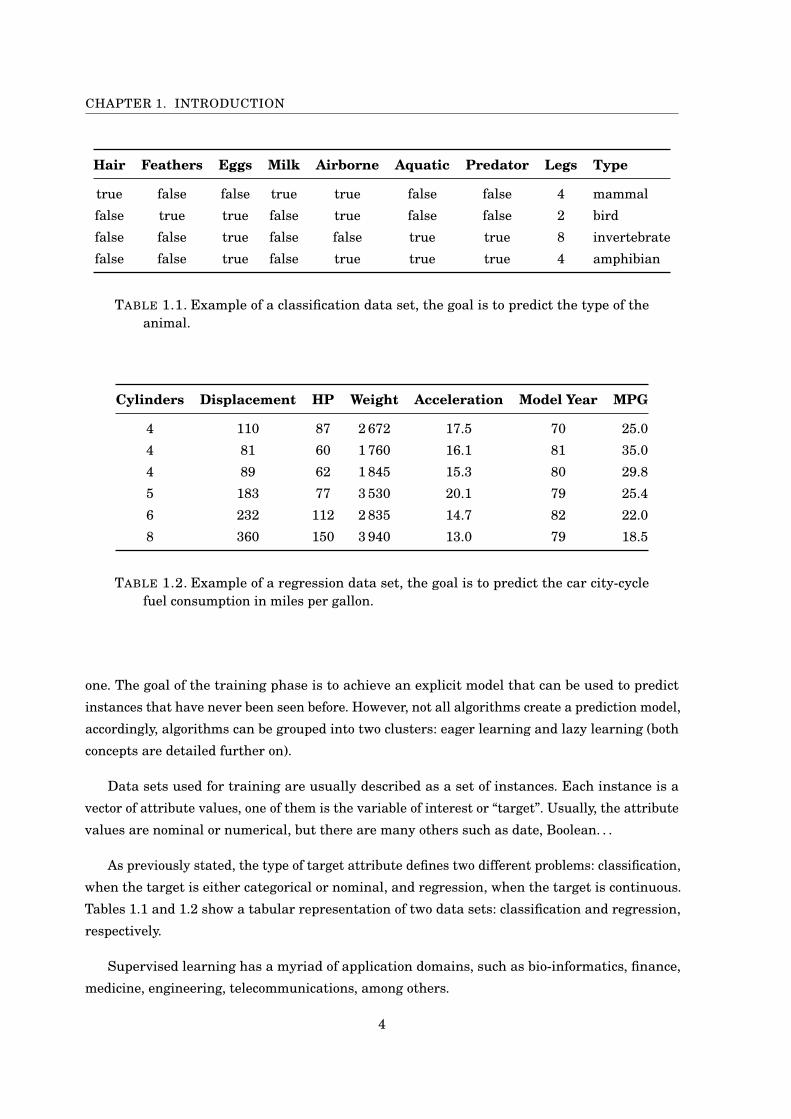
one. The goal of the training phase is to achieve an explicit model that can be used to predict

instances that have never been seen before. However, not all algorithms create a prediction model,

accordingly, algorithms can be grouped into two clusters: eager learning and lazy learning (both

concepts are detailed further on).

Data sets used for training are usually described as a set of instances. Each instance is a

vector of attribute values, one of them is the variable of interest or “target”. Usually, the attribute

values are nominal or numerical, but there are many others such as date, Boolean. . .

As previously stated, the type of target attribute defines two different problems: classification,

when the target is either categorical or nominal, and regression, when the target is continuous.

Tables 1.1 and 1.2 show a tabular representation of two data sets: classification and regression,

respectively.

Supervised learning has a myriad of application domains, such as bio-informatics, finance,

medicine, engineering, telecommunications, among others.

4

1.2. INTRODUCTION TO DATA PREPROCESSING

1.1.1 Lazy learning

Lazy algorithms construct no models throughout the training phase; instead they simply store

the whole data set and postpone its evaluation until a query is submitted; exactly the opposite

procedure to the one that eager algorithms follow.

The advantages and disadvantages of these methods are due to their way of working, as

previously explained. They need large spaces to fit the whole training set and are slow when

they have to evaluate a query. The advantages include a fast training phase (they only store the

whole data set) and good local approximators. Moreover, they can add new examples with no

need for retraining, because they only need to add the new examples to their data base. This last

advantage makes them especially suitable for changing environments, such as concept drift on

streaming learning (Tsymbal, 2004).

Examples of lazy learning algorithms are k nearest neighbours and case-based reasoning,

among others.

1.1.2 Eager learning

Eager algorithms construct a predictive model during the learning phase. The model that is

generated differs according to the algorithm: decision trees, neural networks, etc. The model that

is constructed is used by the algorithm to make predictions when new queries are submitted.

Training instances are used to build the model and, when the training phase ends, the

algorithm only needs the model to decide the target of the new instance. Accordingly, eager

algorithms have no need to store the whole data set, but only the model, which usually requires

much less space. It is commonly named batch or off-line learning, because the training phase is

only done once.

Examples of eager algorithms are those that build decision/regression trees, artificial neural

networks, and support vector machines, among others.

1.2 Introduction to data preprocessing

As previously stated, input data are the cornerstone of Machine Learning. Algorithms need

accurate and well-formed data sets for training purposes. Unfortunately, external factors usually

degrade data consistency in the real world, e.g. presence of noise, superfluous data, huge amount

of instances or features (García et al., 2014). Hence, data preprocessing tasks take up a significant

length of time in Machine Learning work-flows. Two main groups are commonly used to bring

different preprocessing techniques together: data preparation and data reduction.

5


1.2.1 Data preparation

Data preparation gathers several different techniques used to suit data for Data Mining processes

and it is usually a mandatory step. Why is it so important? Imagine a problem of interest: the

data sets have first of all to be gathered from the source or sources and then prepared for use2.

The steps for data preparation are grouped and briefly explained below:

• Data cleaning: includes tasks like noise identification and treatment of missing values. In

a nutshell, the aim of data cleaning is to obtain a well-formed data set suitable to feed

algorithms.

• Data transformation: usually done under human supervision, it comprises such tasks as

discretization, summarization, and aggregation. . .

• Data integration: comprises the processes of merging data from multiple data sources.

Special care must be taken to avoid duplicated instances, and different data domains,

among others.

• Data normalization: different attributes can have different ranges and some methods, such

as distance-based methods, are very sensitive to the scale of the features. Normalization

processes provide the same range and scale for all attributes.

1.2.2 Data reduction

Nowadays, available data sets are progressively increasing in size. As a consequence, many

systems have difficulties when processing (big or huge) data sets to obtain exploitable knowl-

edge (García-Pedrajas and de Haro-García, 2014).

The aim of data reduction is to decrease complexity and to improve the quality of the resulting

data sets by reducing their size. The size of data sets can be reduced in terms of both features

and instances. Some relevant techniques are grouped below:

• Discretization: the process of transforming numerical into discrete attributes. The challenge

is how to find the best ranges or intervals into which the numerical values should be split.

The discretization process can also be considered as part of the data preparation stage.

The decision to include it as a data reduction task is explained in (García et al., 2014):

the discretization stage actually maps data from a large range of numeric values onto a

reduced subset of categorical ones.

• Feature extraction: includes several modifications to the features such as removing one or

more attributes, merging a subset of them, or creating new artificial ones.

2In some cases, the data without preparation could be good enough to feed an algorithm, but its results wouldprobably not make sense.

6

1.3. INSTANCE SELECTION14 1 Introduction

Feature Selection

Instance Selection

Discretization

Fig. 1.4 Forms of data reduction

factors, such as the decreasing of the complexity and improvement of the quality ofthe models yielded, the role of data reduction is again decisive.

As mentioned before, what are the basic issues that must be resolved in datareduction? Again, we provide a series of questions associated with the correct answerrelated to each type of task that belongs to the data reduction techniques:

• How do I reduce the dimensionality of data?—Feature Selection (FS).• How do I remove redundant and/or conflictive examples?—Instance Selection

(IS).• How do I simplify the domain of an attribute?—Discretization.• How do I fill in gaps in data?—Feature Extraction and/or Instance Generation.

In the following, we provide a concise explanation of the four techniques enu-merated before. Figure 1.4 shows an illustrative picture that reflects the forms of datareduction. All of them will be extended, studied and analyzed throughout the variouschapters of the book.

(a) Feature selection

14 1 Introduction

Feature Selection

Instance Selection

Discretization







(b) Instance selection

14 1 Introduction

Feature Selection

Instance Selection

Discretization







(c) Discretization

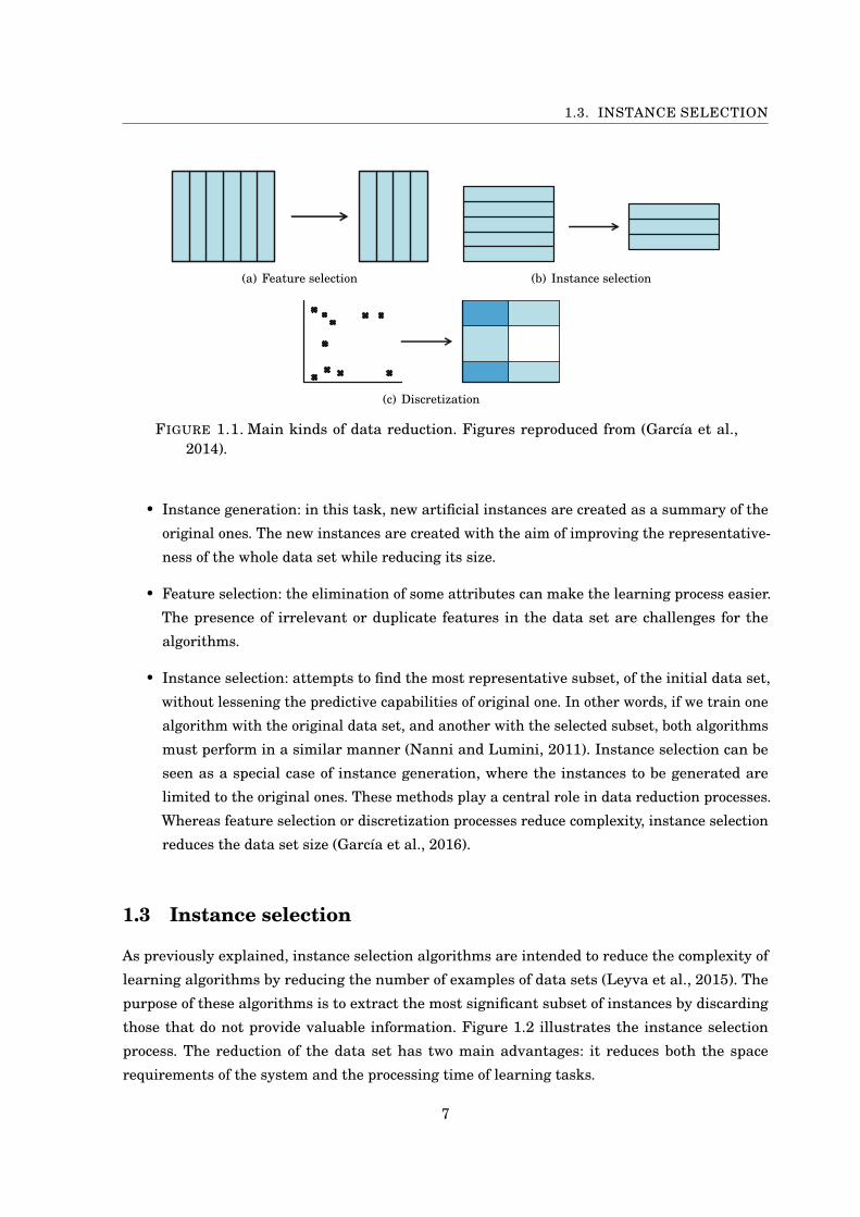
FIGURE 1.1. Main kinds of data reduction. Figures reproduced from (García et al.,2014).

• Instance generation: in this task, new artificial instances are created as a summary of the

original ones. The new instances are created with the aim of improving the representative-

ness of the whole data set while reducing its size.

• Feature selection: the elimination of some attributes can make the learning process easier.

The presence of irrelevant or duplicate features in the data set are challenges for the

algorithms.

• Instance selection: attempts to find the most representative subset, of the initial data set,

without lessening the predictive capabilities of original one. In other words, if we train one

algorithm with the original data set, and another with the selected subset, both algorithms

must perform in a similar manner (Nanni and Lumini, 2011). Instance selection can be

seen as a special case of instance generation, where the instances to be generated are

limited to the original ones. These methods play a central role in data reduction processes.

Whereas feature selection or discretization processes reduce complexity, instance selection

reduces the data set size (García et al., 2016).

1.3 Instance selection

As previously explained, instance selection algorithms are intended to reduce the complexity of

learning algorithms by reducing the number of examples of data sets (Leyva et al., 2015). The

purpose of these algorithms is to extract the most significant subset of instances by discarding

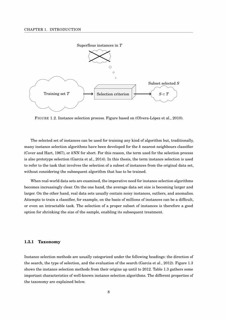
those that do not provide valuable information. Figure 1.2 illustrates the instance selection

process. The reduction of the data set has two main advantages: it reduces both the space

requirements of the system and the processing time of learning tasks.

7


Training set T S ⊂ T

Superflous instances in T

Selection criterion

Subset selected S

FIGURE 1.2. Instance selection process. Figure based on (Olvera-López et al., 2010).

The selected set of instances can be used for training any kind of algorithm but, traditionally,

many instance selection algorithms have been developed for the k nearest neighbours classifier

(Cover and Hart, 1967), or kNN for short. For this reason, the term used for the selection process

is also prototype selection (García et al., 2014). In this thesis, the term instance selection is used

to refer to the task that involves the selection of a subset of instances from the original data set,

without considering the subsequent algorithm that has to be trained.

When real-world data sets are examined, the imperative need for instance selection algorithms

becomes increasingly clear. On the one hand, the average data set size is becoming larger and

larger. On the other hand, real data sets usually contain noisy instances, outliers, and anomalies.

Attempts to train a classifier, for example, on the basis of millions of instances can be a difficult,

or even an intractable task. The selection of a proper subset of instances is therefore a good

option for shrinking the size of the sample, enabling its subsequent treatment.

1.3.1 Taxonomy

Instance selection methods are usually categorized under the following headings: the direction of

the search, the type of selection, and the evaluation of the search (Garcia et al., 2012). Figure 1.3

shows the instance selection methods from their origins up until to 2012. Table 1.3 gathers some

important characteristics of well-known instance selection algorithms. The different properties of

the taxonomy are explained below.

8

1.3. INSTANCE SELECTION

3.2 Prototype Selection Methods

More than 50 PS methods have been proposed in the

literature. This section is devoted to enumerating and

designating them according to a standard followed in this

paper. For more details on their descriptions and

implementations, the reader can visit the webpagehttp://sci2s.ugr.es/pstax associated with this paper. Im-plementations of the algorithms in Java can be found inKEEL software [114].

Table 1 presents an enumeration of PS methods reviewedin this paper. The complete name, abbreviation, andreference are provided for each one. In the case of therebeing more than one method in a row, they were proposedtogether and the best performing method (indicated by therespective authors) is depicted in bold.

3.3 Taxonomy of Prototype Selection Methods

The properties studied above can be used to categorize thePS methods proposed in the literature. The direction of thesearch, type of selection, and evaluation of the search maydiffer among PS methods and constitute a set of propertieswhich are exclusive to the way of operating of the PSmethods. This section presents the taxonomy of PS methodsbased on these properties.

In order to situate the PS methods in time, we illustrate amap of the main methods proposed in each paperenumerated in Table 1. We refer to those which are thepreferred or have reported the best results in the paper inwhich they were proposed as main methods (in otherwords, the ones in bold when more than one method isproposed in a certain paper). Fig. 2 depicts the map of PSmethods. The figure allows us to point out interesting facts:

. Condensation and Edition techniques display oppo-site behavior and they were joined when IB3 wasproposed. IB3 is the first hybrid method whichcombines an edition stage with a condensation one.Since its proposal, there has been a significant effortin proposing new hybrid approaches, decreasing theproposals of condensation methods.

. Few edition methods have been proposed incomparison to the other two families. The mainreasons are that the first edition method, ENN,obtains good results in conjunction with kNN andthe edition approaches do not achieve high reduc-tion rates, which is one of the objects of interest inPS. Incremental edition approaches have not beenproposed because it is very important to know thecomplete set of data for identifying noisy instances.

422 IEEE TRANSACTIONS ON PATTERN ANALYSIS AND MACHINE INTELLIGENCE, VOL. 34, NO. 3, MARCH 2012

TABLE 1PS Methods Reviewed

Fig. 2. Prototype selection map.FIGURE 1.3. Instance selection methods according to the established taxonomy. Figurereproduced from (Garcia et al., 2012).

TABLE 1.3. A brief sample of state-of-the-art instance selection methods as per theaforementioned taxonomy. Computational complexity extracted from (Jankowskiand Grochowski, 2004) and authors’ papers.

Strategy Direction Algorithm Complexity Year Authors

Edition Incremental LSSm O (n2) 2015 Leyva et al. (2015)Decremental ENN O (n2) 1972 Wilson (1972)Batch All-kNN O (n2) 1976 Tomek (1976)

Condensation Incremental CNN O (n3) 1968 Hart (1968)Incremental PSC O (n logn) 2010 Olvera-López et al. (2009a)Decremental RNN O (n3) 1972 Gates (1972)Decremental MSS O (n2) 2002 Barandela et al. (2005)

Hybrid Decremental DROP1-5 O (n3) 2000 Wilson and Martinez (2000)Batch ICF O (n2) 2002 Brighton and Mellish (2002)Batch HMN-EI O (n2) 2008 Marchiori (2008)Batch LSBo O (n2) 2015 Leyva et al. (2015)

9


1.3.1.1 Direction of search

Instance selection can be considered as a search problem; given a particular measure, its goal is

to find the most representative subset of instances for that measure (Cano et al., 2005b). Five

groups may be defined on the basis of the search direction:

• Incremental: they start with an empty data set and add those instances that fulfil a

predefined criterion. Their problem is that they are highly sensitive to the order in which

instances appear. Their main advantages are that data can be processed on stream, they

are usually faster, and they need low storage requirements.

• Decremental: they work in the opposite direction, starting with the whole data set, and

they then remove instances following a predefined criteria. The order is again important,

but not so much as in the previous group. Their main drawback is that the whole data set

has to fit in the memory.

• Batch: instances are analysed in batch mode, i.e. they are processed successively and are

marked for deletion, but the removal process only occurs once at the end of the algorithm.

Their essential advantage is that they retain the overall view of the whole data set at all

times.

• Mixed: they can be seen in between the three previous groups. They start with a predefined

subset, then instances are added or deleted according to certain criterion.

• Fixed: these methods are a sub-family of mixed ones but, in this case, the final instance

number is (as an input parameter of the algorithm) predefined from the outset.

1.3.1.2 Selection strategy

The keystone of the classification process is, forgive the repetition, classification boundaries.

Decision boundaries are formed by instances of two or more different classes that are close to

each other. Accordingly, instances can be either border points (close to boundaries) or central

points3 (far away from boundaries) (Wilson and Martinez, 1997). Figure 1.4 show an example of

two dimensional data set with two classes and 50 instances. The instances found on the decision

boundaries are called border points, while the others are called central points. Three groups are

usually considered in the selection strategy:

• Condensation algorithms: attempt to retain border points, i.e. instances close to the decision

boundaries. They commonly achieve high reduction rates. The problem with these methods,

is that they are highly affected by noisy instances (Jankowski and Grochowski, 2004).

3Some authors, such as Liu and Motoda (2002), consider some other types of points such as critical points andprototypes, although these have been omitted from the taxonomy that is explained here.

10


x1

x2

central points border points central points

FIGURE 1.4. Artificial data set with 50 instances, two features (x1 and x2) and twoclasses (diamond and circle). The decision boundary is the area where both classescome together.

• Edition algorithms: work in the opposite direction, removing border points. They delete

the instances that are not in agreement with their neighbours. They are not interested

in reduction, but in noise elimination. As a result, their reduction rates are lower than

condensation algorithms.

• Hybrid algorithms: as the name suggests, they are somewhere between the above tech-

niques, and their aim is to find the smallest and the most accurate subset of instances.

They remove both central and border instances.

Recently, a new approach that will not fit under any of the previous categories has emerged:

rank methods (Rico-Juan and Iñesta, 2012). These methods sort instances by their importance

(i.e. their usefulness for the classification process), after which, a subset of the best instances is

selected (Valero-Mas et al., 2016).

1.3.1.3 Search Evaluation

Instance selection methods can be grouped according to the strategy used for selecting instances:

either wrappers or filters (Olvera-López et al., 2010).

• Wrapper: the decision either to select or to delete an instance is obtained by a classifier,

usually the kNN.

• Filter: the decision is made by using some heuristics or rules and is not based on a classifier.

11


1.3.2 Computational complexity

As previously stated, instance selection serves to reduce the size of a data set. The complexity of

traditional instance selection algorithms is the main problem in any analysis (García-Osorio et al.,

2010; Silva et al., 2016). As Table 1.3 shows, the computational complexity of the vast majority of

instance selection algorithms is, at least, log-linear. In consequence, a possible solution to manage

increasingly large data sets is their reduction with instance selection methods. Unfortunately,

they are also affected by high computational complexity. Hence, some approaches have recently

emerged that seek to overcome this problem. These different approaches are explained below.

1.3.2.1 Scaling-up approaches

Over the last few years, different approximations have been used to try to adapt instance selection

methods to big/huge data sets. The very first proposal was stratification, used by Cano et al.

(2005a) to boost evolutionary instance selection methods. Their idea consists of splitting the

original data set into disjoint strata (groups or sets of instances) with the same class distribution

as the original one. The scaling-up benefits can be tuned by means of varying the size of each

stratum. Moreover, the stratification process is suitable for boosting any other method. An

improved version of the previous method was presented by de Haro-García and García-Pedrajas

(2009). The beginning of the process is the same: to split the whole data set into disjoint sets.

After the first batch of sets have been processed, the selected instances by the algorithm are

joined, and the process starts again.

A more novel and remarkable approach (because of its performance) was proposed by García-

Osorio et al. (2010). The process is performed in a predefined number of rounds r. In each round,

a partition splits the whole data set into different disjoint subsets, also called bins. As in the

previous approaches, an instance selection algorithm is performed over every single bin. The

algorithm updates an array of votes by increasing them by one if the instance has been selected.

After performing a predefined number of rounds, the array of votes is used to determine, by

means of a threshold, which instances should be either selected or removed.

Other works, such as (Angiulli and Folino, 2007), have focused on developing a distributed

method for computing a consistent subset of very large data sets.

1.3.3 Most common methods

It has been noted in the current chapter that a great number of instance selection algorithms

already exist and many others are presented every year. The most influential instance selection

algorithms according to García et al. (2016) are depicted below: Condensed Nearest Neighbour

(CNN), Edited Nearest Neighbour (ENN), Decremental Reduction Optimization (DROP) and

Iterative Case Filtering (ICF). An application of the aforementioned methods to a subsample of

the banana data set shows the selected subsets in Figure 1.5.

12


0 0.2 0.4 0.6 0.8 10

0.2

0.4

0.6

0.8

1

x1

x 2

(a) Banana data set: 1 326 instances

0 0.2 0.4 0.6 0.8 10

0.2

0.4

0.6

0.8

1

x1

x 2

(b) CNN: 307 instances

0 0.2 0.4 0.6 0.8 10

0.2

0.4

0.6

0.8

1

x1

x 2

(c) ENN: 1 168 instances

0 0.2 0.4 0.6 0.8 10

0.2

0.4

0.6

0.8

1

x1

x 2

(d) DROP3: 144 instances

0 0.2 0.4 0.6 0.8 10

0.2

0.4

0.6

0.8

1

x1

x 2

(e) ICF: 176 instances

FIGURE 1.5. Subsample of Banana data set filtered with the most influential instanceselection methods according to García et al. (2016): CNN, ENN, DROP3 and ICF.

13


1.3.3.1 Condensed Nearest neighbour

The algorithm of Hart (1968), Condensed Nearest Neighbours (CNN) is considered the first formal

proposal of instance selection for the nearest neighbour rule. The concept of consistency with

respect to the training set is important in this algorithm, and is defined as follows: given a

non-empty set X (X 6= ;), a subset S of X (S ⊆ X ) is consistent with respect to X if, using the

subset S as a training set, the nearest neighbour rule can correctly classify all the instances in X .

Following this definition of consistency, if we consider the set X as the training set, a condensed

subset should have the properties of being consistent and should, ideally, be smaller than X .

Algorithm 1 shows the structure of the method. It starts with a data set, S, initially with only

one randomly selected instance (alternatively, S could have one randomly selected instance per

class in the data set). Then, it attempts to classify all the instances of X by using the instances

in S, according to the nearest neighbour rule. If it is successful, the algorithm proceeds with

the next instance, otherwise the misclassified instance is added to S and the verification of the

correct classification of X starts from the beginning once again. It will eventually terminate,

returning S as a selected data set.

Algorithm 1: Condensed Nearest Neighbour (CNN)Input: A training set X = {(x1, y1), ..., (xn, yn)}Output: The set of selected instances S ⊆ X

1 S = {x1}2 foreach x ∈ X do3 if x is misclassified using S then4 Add x to S5 Restart

6 return S

1.3.3.2 Edited Nearest Neighbour

The first proposal for editing data sets was presented by Wilson (1972) with the name of Edited

Nearest Neighbour (ENN). It is a decremental method, thus it starts with the whole data set X ,

and each instance is removed, if it is not well classified by its k nearest neighbours. The number

of nearest neighbours, k, is a parameter of the algorithm. In the original paper, k was set to 3.

Algorithm 2 shows its pseudocode. ENN removes noisy as well as border instances, achieving

neater decision boundaries. Moreover, central instances are unaffected by the editing process.

The goal of this algorithm is not the reduction of data set, but to improve the accuracy of the

selected subset. Due to its cleaning capabilities, it has been used by many other algorithms for

noise filtering (e.g. DROP3, ICF. . . ).

14


Algorithm 2: Edited Nearest Neighbours (ENN)Input: A training set X = {(x1, y1), ..., (xn, yn)}, the number of nearest neighbours kOutput: The set of selected instances S ⊆ X

1 S = X2 foreach x ∈ S do3 if x is misclassified using its k nearest neighbours then4 Remove x to S

5 return S

c

a

b

d

Figure 1.6: Representation of nearest neighbour and associate relations in a two dimensionalspace: each point represents an instance, there are two different classes (black and white), andk = 3. The nearest neighbours of a are {b,c,d}, so a is an associate for b,c, and d.

1.3.3.3 Decremental Reduction Optimization Procedure

The DROP (Decremental Reduction Optimization Procedure) family of algorithms (Wilson and

Martinez, 2000) comprises some of the best instance selection methods for classification (Brighton

and Mellish, 2002; Olvera-López et al., 2009b; Pérez-Benítez et al., 2015). The instance removal

criterion is based on two concepts: associates and nearest neighbours. The relation of associate

is the opposite of nearest neighbour: an instance p that has q as one of its nearest neighbours

is referred to as an associate of q. The set of nearest neighbours of one instance is called

neighbourhood. The set of associates for each instance is a list with all instances that have that

particular instance in their neighbourhood. Figure 1.6 shows a two dimensional data set with

two classes (black and white points). The k nearest neighbours of a, for k = 3, are {b,c,d}. This

means that a is an associate of the instances of b,c and d .

The pseudocode of DROP3 is described in Algorithm 3. It begins with a noise-filter (similar

to ENN), after which, the instances are sorted in order of the distance to their nearest enemy.

The lists of nearest neighbours and associates are calculated for each instance. Then, on the

main loop of the algorithm, for each instance x, with contains the number of associates of x that

are correctly classified when x is kept in the data set, whereas without contains the number of

associates that are correctly classified when x is removed from the data set. If without is greater

than or equal to with, the instance x is removed, because its elimination will not influence the

15


classification of its associates. If x is removed, all of its associates need to update their neighbour

list.

Algorithm 3: Decremental Reduction Optimization Procedure 3 (DROP3)Input: A training set X = {(x1, y1), ..., (xn, yn)}, the number of nearest neighbours kOutput: The set of selected instances S ⊆ X

1 Noise filtering: remove any instance in X misclassified by its k neighbours2 S = X3 Sort instances in S by the distance to their nearest enemy4 foreach instance x ∈ S do5 Find x.N1...k+1, the k+1 nearest neighbours of x in S6 Add x to each of its neighbour’s list of associates

7 foreach instance x ∈ S do8 Let with= # of associates of x correctly classified by x as a neighbour9 Let without= # of associates of x correctly classified without x

10 if without≥ with then11 Remove x from S12 foreach associate a of x do13 Remove x from a’s list of nearest neighbour14 Find a new nearest neighbour for a15 Add a to its new neighbour’s list of associates

16 return S

1.3.3.4 Iterative Case Filtering

The selection rule of the Iterative Case Filtering algorithm (Brighton and Mellish, 2002), or ICF

for short, uses two concepts: coverage and reachable. These two concepts are closely related to the

neighbourhood and associate lists used by the DROP algorithms. The coverage of an instance is

its neighbourhood but, instead of considering a fixed number of neighbours, k, all instances closer

than its closest enemy are within its coverage set4. The reachable set of an instance is the set of

all instances for which that particular instance is within their coverage set. Figure 1.7 represents,

in a two dimensional space, the previous concept. The example is formed of six instances (points)

that belong to two different classes (black and white). The dashed circle centred in a is the

boundary of its local set, c is the nearest enemy of a, and the distance between both instances

defines the radius of the local set of a.

The deletion rule is as follows: if the cardinality of the reachable set of an instance (its set of

associates) is bigger than its coverage (its neighbourhood), the instance is removed from the data

set. So, if another object generalizes the information of that instance, the algorithm will remove

4The local or coverage set is formed by the group of instances included in the largest hypersphere centred on aninstance such that all of them are of the same class (Leyva et al., 2015).

16


c

a

b

Figure 1.7: Representation of the local set in a two dimensional space: each point represents aninstance, and there are two different classes (black and white). As the nearest enemy of a is c,the local set of a is composed of a and b: LocalSet(a)= {a,b}.

it. The ICF algorithm begins with a noise-filtering stage that addresses the drawbacks of noisy

data sets, in the same way as DROP3.

There are two stages in the ICF: i) noise filter, and ii) selection process (see Algorithm 4).

First of all, it removes noisy instances from the original data set. Then, both the coverage and

the reachable sets are calculated for each instance. On the main loop, the method checks the

cardinality of reachable and coverage (for each instance). If one instance has |reachable| >|coverage|, it is marked for removal; once they have been evaluated, those marked for removal

are deleted. This process continues until no further instance will be removed.

Algorithm 4: Iterative Case Filtering (ICF)Input: A training set X = {(x1, y1), ..., (xn, yn)}, the number of nearest neighbours kOutput: The set of selected instances S ⊆ X

1 S = X2 Noise filtering: remove any instance in S misclassified by its k neighbours3 repeat4 foreach instance x ∈ S do5 Compute coverage(x)6 Compute reachable(x)

7 progress = False8 foreach instance x ∈ S do9 if |reachable(x)| > |coverage(x)| then

10 Flag x for removal11 progress = True

12 foreach instance x ∈ S do13 if x flagged for removal then14 S = S− {x}

15 until not progress16 return S

17


1.3.4 Big data

In recent years, the massive growth in the volume of databases has led to the coining of the new

term: big data. The definition of the new term is not clear, although Laney (2001) described it as

the opportunities and difficulties that appear, as data volumes and variety and processing speeds

increase. Another possible, and common, definition for big data is the difficulties and problems

that emerge when the amount of data for processing exceeds the capabilities, memory and/or

time, of a given system (Minelli et al., 2012).

Big data faces the problems associated with these types of data sets at various levels: firstly,

we need implementations that, with regard to the computational complexity of the algorithms,

are scalable and that run in linear time; at the level of methodologies, we are looking for a means

of designing algorithms that can be executed in parallel on groups of computers, a task that

is suited to MapReduce (Dean and Ghemawat, 2008); and, finally, at a technological level, we

seek frameworks that provide a series of APIs and data structures that facilitate the work of

implementing algorithms, for which purpose Spark (Zaharia et al., 2010) and Hadoop (White,

2009) have proven their worth.

Efficient methods are needed to process increasingly massive data sets, and an intuitive

solution to cope with them is their size reduction. Instance selection has shown itself to be effective

for this task, by reducing the size of the data sets while preserving their predictive capabilities.

The problem that emerges at this point, as previously explained, is the high computational

complexity that these methods have.

Recently, some studies have focused on instance reduction for big data, both on instance

selection (Triguero et al., 2015) and on instance generation (Triguero et al., 2014). However, as

García et al. (2016) remarked, more scalable methods are required for instance selection with the

aim of tackling the current size of data sets.

1.4 Experimental methodology

Instance selection algorithms serve to reduce the size of data sets and to select the most repre-

sentative possible subset. The task must be considered as a multi-objective problem: on the one

hand, reduction and, on the other, accuracy. Both objectives, nonetheless, are usually in opposite

directions (Leyva et al., 2015). This section presents the most common methodology used in the

instance selection literature.

1.4.1 Model validation

Estimation of the accuracy of a predictive model (classifier or regressor) when using the selected

subset is necessary for the evaluation of instance selection algorithms. If the accuracy of the model

is to be properly estimated, then an estimation method with low bias and low variance (Kohavi,

1995) is necessary. Some of the most common estimation methods are presented here; the reason

18

1.4. EXPERIMENTAL METHODOLOGY

test data training data

all data

Iteration 1

Iteration 2

Iteration 3

Iteration 4

FIGURE 1.8. Diagram of k-fold cross-validation with k = 4. Each dot represents aninstance and the colour defines the class.

why there are so many methods is because all of them fail under certain conditions (Schaffer,

1994).

1.4.1.1 Holdout

Holdout estimation, or test sample estimation, is performed in a simple manner by splitting the

original data set into two disjoint subsets: a training set and a test (or holdout) set. A common

configuration for this method is to use 2/3 of the original data set for training, and the remaining

1/3 for testing. The main problem with this method is that the data may not be properly used for

training, because one third of the original data set is missing.

1.4.1.2 Cross-validation

Commonly referred to as k-fold cross-validation, or rotation estimation, this method splits the

original data set into k disjoint sets (or folds) of approximately equal size. The learner is trained

k times, using k−1 folds for training, and the remaining fold is used for testing. Training and

testing sets are interchanged throughout the execution as can be seen in Figure 1.8.

A complete cross-validation would require all possible combinations to be tested, which is too

expensive to apply in practice, so a number of 10 folds is commonly used (McLachlan et al., 2005).

1.4.2 Performance measures

When researchers wish to analyse an instance selection method, three measures are typically

taken into account: accuracy, compression and computational complexity. Despite the fact that an

ideal method would maximize accuracy and compression, as quickly as possible, all these goals

often work in opposing directions (Leyva et al., 2015). All of these measures are briefly discussed

below.

19


Notation Name Example

O (1) Constant Determine whether a number is even or oddO (logn) Logarithmic Find an item in a sorted vector of size n by using binary searchO (n) Linear Compute the arithmetic mean of a vector of size nO (n logn) Loglinear An average case of sorting a vector of size n by using quicksortO (n2) Quadratic Compute the 1 nearest neighbour of a data set with n instances

TABLE 1.4. Summary of common computational complexities expressed in “Big O”notation.

N

n

O (n)O (n2)

O (logn)

O (n logn)

O (1)

FIGURE 1.9. Number of operations according to the computational complexity. N is thenumber of operations and n the size of the input data set.

1.4.2.1 Computational complexity

Computational complexity is usually expressed in “Big O” notation. It represents the response (in

time) of the algorithm to changes in the input size. It is an asymptotic notation that facilitates a

comparison of the different growth rates of various methods. It is also a means of showing the

increased time that the algorithm requires when the data sets become larger.

Table 1.4 shows a brief list of common computational complexities expressed in the stated

notation. Figure 1.9 offers a graphical representation of the number of operations that correspond

to different computational complexities as the data sets grow in size.

20


Predicted conditionPositive prediction Negative prediction

Actual Positive class True positive (TP) False negative (FN)condition Negative class False positive (FP) True negative (TN)

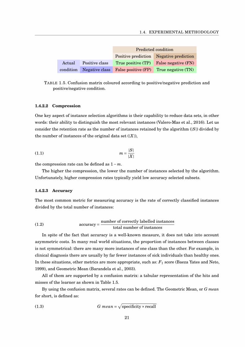
TABLE 1.5. Confusion matrix coloured according to positive/negative prediction andpositive/negative condition.

1.4.2.2 Compression

One key aspect of instance selection algorithms is their capability to reduce data sets, in other

words: their ability to distinguish the most relevant instances (Valero-Mas et al., 2016). Let us

consider the retention rate as the number of instances retained by the algorithm (|S|) divided by

the number of instances of the original data set (|X |),

(1.1) m = |S||X |

the compression rate can be defined as 1−m.

The higher the compression, the lower the number of instances selected by the algorithm.

Unfortunately, higher compression rates typically yield low accuracy selected subsets.

1.4.2.3 Accuracy

The most common metric for measuring accuracy is the rate of correctly classified instances

divided by the total number of instances:

(1.2) accuracy= number of correctly labelled instancestotal number of instances

In spite of the fact that accuracy is a well-known measure, it does not take into account

asymmetric costs. In many real world situations, the proportion of instances between classes

is not symmetrical: there are many more instances of one class than the other. For example, in

clinical diagnosis there are usually by far fewer instances of sick individuals than healthy ones.

In these situations, other metrics are more appropriate, such as: F1 score (Baeza Yates and Neto,

1999), and Geometric Mean (Barandela et al., 2003).

All of them are supported by a confusion matrix: a tabular representation of the hits and

misses of the learner as shown in Table 1.5.

By using the confusion matrix, several rates can be defined. The Geometric Mean, or G mean

for short, is defined as:

(1.3) G mean =√

specificity×recall

21


where

(1.4) specificity= TNTN +FP

(1.5) recall= TPTP +FN

F1 score (F-measure or F-score) is the Harmonic mean of precision and recall:

(1.6) F1 measure= 2× precision×recallprecision+recall

where

(1.7) precision= TPTP +FP

1.4.3 Statistical comparisons

Statistical tests have become an essential tool for comparing different methods with the aim of

determining whether one method (or more) is significantly better than the others (Derrac et al.,

2011). Commonly, experiments used to check whether one method is better than another involve

several data sets. The results of methods for the different data sets are the observations, which

are compared by means of statistical tests5. The tutorial proposed by Derrac et al. (2011) was

followed in this section.

According to the capability of tests to compare two or more methods, statistical tests can be

sorted into two different groups: pairwise (one vs. one) and multiple comparisons (all vs. all).

1.4.3.1 Pairwise comparisons

These comparators are the simplest ones, only able to compare two different algorithms.

• The Sign test: begins by separately counting the wins and losses. These counters are used in

inferential statistics with a two-tailed binomial test. The null hypothesis states that if each

of the two algorithms wins on approximately n/2 out of n datasets then both algorithms are

equivalent. By using the z test, it can be determined whether one algorithm is significantly

better than the other. A specific definition would be as follows: if the number of wins of

one algorithm is, at least, n/2+1.96 ·pn /2, then that algorithm is significantly better (at a

confidence level of 0.05) than the other.

5The statistical tests explained and used in this thesis are non-parametric or distribution-free tests.

22


• The Wilcoxon signed rank test: more powerful and therefore preferable to the previous

Sign Test. It starts by computing the differences between the scores of both algorithms (di)

and takes no account of a pair of scores, if the difference between both scores is zero. These

differences are ranked according to their absolute values and, in case of a tie, both ranks

are summed up and divided by two. So, let R+ be the sum of ranks when the first algorithm

is better than the second and let R− be the opposite.

(1.8) R+ = ∑di>0

rank(di)+ 12

∑di=0

rank(di)

(1.9) R− = ∑di<0

rank(di)+ 12

∑di=0

rank(di)

The result of the test is calculated by comparing the minimum value between R+ and R−

(T =min(R+,R−)) and the Wilcoxon distribution for n degrees of freedom. So, one algorithm

will outperform the other, if T is less than or equal to the value of the Wilcoxon distribution

for n degrees of freedom.

1.4.3.2 Multiple comparisons

When more than two algorithms are compared, the previously explained methods are no longer

useful. There are other specifically designed methods to tackle these situations. In 1×N compar-

isons, one method is taken as the control method, and the other methods are compared against

it. Moreover, N ×N comparisons consider all possible combinations between all methods at the

same time.

• Average ranks: rather than a statistical comparison itself, average ranks is included here

because it is commonly used in combination with the other tests described below. Average

ranks are calculated as follows: the results of the methods are ordered according to the

measure of interest. A value of 1 is assigned to the best method, the value 2 to the second

best, and so on. In the case of a tie, values of the ranks are added up and divided by the

number of methods that have tied. Once the ranking of each data set and algorithm has

been calculated, the average for each method is computed. The closer the ranking is to one,

the better the method.

• The Friedman Test: a nonparametric procedure with similarities to ANOVA (ANalysis

Of VAriance). The null hypothesis is that the medians of the samples are equal. The test

begins with a calculation of the average ranks explained above. The null hypothesis states

23


that all algorithms perform similarly, if the ranks are equal. The Friedman statistic F f is

computed as:

(1.10) F f =12n

k(k+1)

[∑j

R2j −

k(k+1)2

4

]

where n is the number of data sets, k is the number of models to be compared, and R j is

the average rank of the model j. F f must be compared with a χ2 distribution with k−1

degrees of freedom6.

• Iman-Davenport’s Test (Iman and Davenport, 1980): uses a modified statistic to avoid the

undesired conservative effect of the Friedman test. The statistic is computed as

(1.11) FID = (n−1)F j

n(k−1)−F j

FID must be compared with F distribution with k−1 and (k−1)(N −1) degrees of freedom.

1.4.3.3 Post-hoc procedures

The methods explained above are able to detect significant differences over all of the methods,

however, they are unable to compare two methods by themselves properly. This drawback is the

reason for the widespread use of post-hoc procedures.

A family of hypotheses can be defined for the purpose of drawing a comparison between one

control method and some others. Post-hoc procedures offer a p-value to determine whether or not

the hypothesis can be rejected.

For each nonparametric test, a conversion of the rankings is defined by using a normal

approximation. Equation 1.12 shows the z computation for the Friedman test.

(1.12) z = (Ri −R j)/

√k(k+1)

6n

where Ri and R j are the average ranks of the algorithms that are compared.

6When n and k are large enough, Derrac et al. (2011) proposed n > 10 and k > 5, but exact critical values must beused for a smaller number of n and k (Sheskin, 2003).

24

Instance-based learning algorithms sufferfrom several problems.

Aha et al. (1991)

CH

AP

TE

R

2MOTIVATION AND GOALS

Having introduced the theoretical background of the thesis in the preceding chapter, the

rationale for this work is described below. The main goal of this thesis is the design of

new methods and their improvement, so as to apply instance selection algorithms in

under-explored areas, such as regression problems and huge data sets. All the chapters that are

referenced hereinafter are from Part II – Publications.

• Despite the fact that instance selection for classification has been broadly researched over

the last decades, instance selection methods for regression task has not aroused as much

interest. The difficulties associated with this task are the main reasons. Chapters 1 and 3

present new instance selection methods designed specifically for regression.

• In the same way that the combination (ensemble) of either multiple classifiers or regressors

offers better performances than those methods by themselves (Kuncheva, 2004), the idea of

merging instance selection methods for regression is presented and tested in Chapter 2.

• As previously outlined, the computational complexity of instance selection methods means

that they are unable to be used with big or huge data sets. Although recent works have

been developed to scale up instance selection methods, all of them are based on the divide-

and-conquer idea. Chapter 4 addresses the problem of instance selection on huge data sets

from a new point of view. The use of locality sensitive hashing, LSH for short (Leskovec

et al., 2014), means data sets may be processed extremely quickly in one pass. The new

method is of linear complexity in relation to the number of instances.

25

Any sufficiently advanced technology isindistinguishable from magic.

Arthur C. Clarke

CH

AP

TE

R

3DISCUSSION OF RESULTS

The most valuable aspect of research is communication and dissemination. The research

performed during this thesis is no exception and has yielded valuable results in the form

of journal papers, congress communications, and other informal communications. All of

these contributions are listed below, however only journal papers are compiled as chapters in

Part II of the present thesis.

3.1 Journal papers

1. Instance selection for regression by discretization.

Authors: Álvar Arnaiz-González, José F. Díez-Pastor, Juan J. Rodríguez, César Ignacio

García-Osorio.

Published in: Expert Systems With Applications (Q1).

Year: 2016.

2. Instance selection for regression: Adapting DROP.


García-Osorio.

Published in: Neurocomputing (Q1).

Year: 2016.

3. Fusion of instance selection methods in regression tasks.

Authors: Álvar Arnaiz-González, Marcin Blachnik, Mirosław Kordos, César García-Osorio.

27

CHAPTER 3. DISCUSSION OF RESULTS

Published in: Information Fusion (Q1).

Year: 2016.

4. Instance selection of linear complexity for big data.

Authors: Álvar Arnaiz-González, José F. Díez-Pastor, Juan J. Rodríguez, César García-

Osorio.

Published in: Knowledge-Based Systems (Q1).

Year: 2016.

3.2 Non-indexed journals and other communications

1. MR-DIS: Democratic Instance Selection for big data by MapReduce.

Authors: Álvar Arnaiz-González, Alejandro González-Rogel, José F. Díez-Pastor, Carlos

López-Nozal

Published in: Progress in Artificial Intelligence.

Year: 2017.

2. MR-DIS – a scalable instance selection algorithm using MapReduce on Spark.

Authors: Álvar Arnaiz-González, Alejandro González-Rogel, Carlos López-Nozal.

Published in: ERCIM News.

Year: 2017.

3. Study of instance selection methods (poster).

Authors: Álvar Arnaiz-González.

Presented in: INIT/AERFAI 2017 – Summer School on Machine Learning.

Year: 2017.

3.3 Conference papers

1. Selección de instancias en regresión mediante discretización (Instance selection for regres-

sion by means of discretization).


García-Osorio.

Published in: ESTYLF 2014 – XVII Congreso Español Sobre Tecnologías y Lógica Fuzzy.

Year: 2014.

28

3.4. SOURCE CODE REPOSITORY

2. LSH-IS: Un nuevo algoritmo de selección de instancias de complejidad lineal para grandes

conjuntos de datos (LSH-IS: A new instance selection algorithm of linear complexity for

huge data sets).

Authors: Álvar Arnaiz-González, José F. Díez-Pastor, César Ignacio García-Osorio, Juan J.

Rodríguez.

Published in: CAEPIA 2015 – XVI Conferencia de la Asociación Española para la In-

teligencia Artificial.

Year: 2015.

3. Enfoque MapReduce para el democratizado de métodos de selección de instancias (MapRe-

duce approach for the democratization of instance selection algorithms).

Authors: Alejandro González-Rogel, Álvar Arnaiz-González, Carlos López Nozal, José F.

Díez-Pastor.

Published in: CAEPIA 2016 – XVII Conferencia de la Asociación Española para la In-

teligencia Artificial.

Year: 2016.

3.4 Source code repository

In science, it is important to be able to reproduce studies made by other researchers. As Collberg

and Proebsting (2016) said: “Reproducibility is a cornerstone of the scientific process”. With this

in mind, the source code of the different algorithms designed and developed for the thesis are

publicly available at the GitHub repository on: https://github.com/alvarag/.

29

https://github.com/alvarag/

It is impossible to compile a list of themost significant achievements in the pastdecade without offending or alienatinghalf of my readership. I will leave thistask to the main judge – time.

Kuncheva (2004)

CH

AP

TE

R

4CONCLUSIONS

A study of instance selection methods is presented in this thesis. Their contributions can

be grouped into two main problems: classification and regression. A summary of the chief

contributions are listed below.

4.1 Regression

The lack of instance selection methods for regression (Kordos and Blachnik, 2012) sparked my

initial interest in this task. The first idea to address this gap was discretization, which consists

in transforming the continuous output variable into discrete counterparts. The proposal was

tested as a noise filter against two state-of-the-art instance selection methods for noise reduction,

both of which were prepared to process regression problems. The results showed a very good

performance on noise identification, accuracy and compression. Moreover, the proposed meta-

model can not only be used for noise filtering, but for adapting any other instance selection

classification algorithm.

The DROP family, presented by Wilson and Martinez (2000), contains some of the best instance

selection techniques and is now considered a standard for instance-based learning (García et al.,

2016). Hence, our aim was to adapt these methods for regression, to test whether the adaptation

inherits the same beneficial behaviour in regression. Two different approaches addressed the

adaptation and both were empirically tested. The results were competitive and, additionally, the

robustness of the method in the presence of noise was assessed.

Finally, the combination of several instance selection methods for regression was evaluated. A

bagging-like process was presented and evaluated against different algorithms. The experimental

study concluded that the combination gave better results than the method by itself, i.e. this study

upheld the ‘ensemble’ thesis.

31

CHAPTER 4. CONCLUSIONS

4.2 Classification

Given the aforementioned computational complexity of the traditional instance selection methods,

a couple of new algorithms for huge data sets were proposed. The proposal is able to cope with

vast amounts of data due to its linear complexity in relation to the number of instances. The new

methods are not only faster than state-of-the-art algorithms, but they are also competitive in

terms of accuracy. One of the proposed algorithms is able to process instances on fly, with no

need to fit the whole data set into the memory, which makes it specially suitable for big data

environments.

The problems that emerge with big data are diverse. We have centred on the lack of instance

selection methods that are able to cope with big data. We focused on of the most popular

methods, the Spark framework, which bases its performance on the MapReduce model (Dean

and Ghemawat, 2008). With this in mind, we designed and implemented a parallel version of one

instance selection method called Democratic Instance Selection (DIS) by following the MapReduce

model. The results were satisfying and the method was tested in a big data environment by using

the Cloud Dataproc1 Google services.

1Main page of Google Cloud Dataproc available on https://cloud.google.com/dataproc/.

32

https://cloud.google.com/dataproc/

Anyone who has never made a mistakehas never tried anything new.

Albert Einstein

CH

AP

TE

R

5FUTURE LINES

Instance selection is a research topic of great interest nowadays, as is evident from the

numerous papers on the topic, frequently published in scientific journals. Researchers are

engaged with both lines of investigation that form the central focus of this thesis: instance

selection for regression (Song et al., 2017) and instance selection for big data (Si et al., 2017).

As a result, the future lines of the research are twofold: on the one hand, to improve current

instance selection methods for regression; and, on the other hand, to research new methods and

to develop them so that they are able to manage extremely large data sets.

5.1 Regression

Three journal papers on instance selection for regression are compiled in this thesis. However

there is still a lot of room for improvement, mainly related with the complexity of the methods. All

of the algorithms that were implemented are based on traditional instance selection classification

algorithms, so their complexity is at least exponential, O (n2). The reduction of their complexity is

a pressing topic and urgently required, due to the fast growth of real data sets. This is particularly

important for industrial applications, as Kordos and Blachnik (2012) has noted, because there

are massive regression data sets, which require faster and more effective reduction techniques.

5.2 Big data

In accordance with big data environments, the design and study of new methods (or the im-

provement of existing ones) are essential. Data sets are getting larger and larger, as previously

explained, but there are still only a few instance selection methods capable of dealing with

them. Even though some data reduction techniques of low complexity have emerged in recent

33

CHAPTER 5. FUTURE LINES

e-mailspam? No

e-mailspam? No

e-mailspam? Yes

e-mailspam? Yes

e-mailspam? Yes

animalMammal

animalMammal

animalReptile

animalReptile

animalFish

animalFish

Figure 5.1: Visual examples of single-label data sets: binary on the left and multi-class on theright. Dashed lines represent the boundaries between classes.

years (Olvera-López et al., 2009a; Silva et al., 2016), their implementation into big data frame-

works are not available. This means they can neither be used on real-world data sets, nor

compared with the few existing implementations.

5.3 Multi-label

There is a new topic where the usefulness of instance selection is starting to become apparent:

multi-label learning. In the same way as single-label classification seeks to assign a label to

an instance for which the label is unknown, multi-label classification presents a similar task.

The difference between them is that instances have a collection of labels, known as labelset,

rather than only one. This peculiarity implies a much more difficult task, because there are

hidden relationships between labels that must be taken into account. So far, there are only

a couple of works in which instance selection has been used for multi-label data sets (Charte

et al., 2014; Kanj et al., 2016). For this reason, my ongoing research is an attempt to design new

instance-selection methods that are capable of processing multi-label data sets. Figure 5.1 shows

a couple of examples of single-label data sets, with two (binary) and more classes. Figure 5.2

shows an example of a multi-label data set.

The work on this topic during the last year has already borne fruit, as a result the following

couple of papers were submitted to indexed journals. The reviewers’ answer of the first paper has

not yet arrived. In regard to the second one, it is currently being reviewed.

• “Binary relevance approach for multi-label instance selection”.

• “The extension of local sets to multi-label classification provides good instance selection

methods”.

34

5.4. MULTI-TARGET REGRESSION

Tree label

Mountain label

Water labelimage

Mountain? YesWater? YesTree? Yes

image

Mountain? YesWater? NoTree? No

image

Mountain? NoWater? NoTree? No

image

Mountain? NoWater? YesTree? No

Figure 5.2: Visual example of a multi-label data set and its boundaries. Each of the four picturesis an instance and there are three classes: mountain, water, and tree. Dashed and dotted linesrepresent the boundaries between individual classes.

5.4 Multi-target regression

A topic closely related to multi-label is multi-target regression. Whereas each instance in multi-

label learning has a set of labels, each instance in multi-target data sets has a set of numeric

values (Appice and Džeroski, 2007). In other words, the aim of Multi-target regression is the

simultaneous prediction of multiple target variables for each instance (Spyromitros-Xioufis et al.,

2012).

There are many real-world problems to which multi-target regression can be applied. The typ-

ical example from the environmental sciences involves the prediction of the distribution structure

of species in an environment (Demšar et al., 2006). Other areas where multi-target regression is

commonly used are bio-informatics and medicine, among others (Appice and Džeroski, 2007). As

in multi-label, instance selection for multi-target regression is yet to be researched.

35

Part II

Publications

Simple rules survive.

Devroye et al. (1996)

CH

AP

TE

R

1INSTANCE SELECTION FOR REGRESSION BY DISCRETIZATION

This journal paper presents the idea of using the discretization process with the aim of

adapting instance selection algorithms for classification to regression. The meta-model

process is presented, so that any instance selection method can be used. The concept

in the paper is an adaptation of the Wilson Edition algorithm (ENN (Wilson, 1972)) that is

tested against two instance selection methods for regression: MI (Guillen et al., 2010) and

RegENN (Kordos and Blachnik, 2012). Both methods are noise filters, so the experiments were

carried out by adding artificial noise. In addition to their comparison in terms of accuracy and

compression (conventional instance selection measures), their identification of noise instances is

also evaluated by considering a binary problem.

Authors: Álvar Arnaiz-González, Jose-Francisco Díez-Pastor, Juan José Rodríguez-Diez, César

Ignacio García-Osorio

Type: Journal

Published in: Expert Systems with Applications 54: 340 – 350

Year: 2016

Reference: Arnaiz-González et al. (2016b)

39

Instance selection for regression by discretization

Alvar Arnaiz-Gonzalez, Jose F. Dıez-Pastor, Juan J. Rodrıguez, Cesar Garcıa-Osorio

University of Burgos, Spain

Abstract

An important step in building expert and intelligent systems is to obtain the knowledgethat they will use. This knowledge can be obtained from experts or, nowadays moreoften, from machine learning processes applied to large volumes of data. However, forsome of these learning processes, if the volume of data is large, the knowledge extractionphase is very slow (or even impossible). Moreover, often the origin of the data sets usedfor learning are measure processes in which the collected data can contain errors, so thepresence of noise in the data is inevitable. It is in such environments where an initialstep of noise filtering and reduction of data set size plays a fundamental role. For bothtasks, instance selection emerges as a possible solution that has proved to be useful invarious fields. In this paper we focus mainly on instance selection for noise removal. Inaddition, in contrast to most of the existing methods, which applied instance selection toclassification tasks (discrete prediction), the proposed approach is used to obtain instanceselection methods for regression tasks (prediction of continuous values). The differentnature of the value to predict poses an extra difficulty that explains the low number ofarticles on the subject of instance selection for regression.

More specifically the idea used in this article to adapt to regression problems “classic”instance-selection algorithms for classification is as simple as the discretization of thenumerical output variable. In the experimentation, the proposed method is comparedwith much more sophisticated methods, specifically designed for regression, and showsto be very competitive.

The main contributions of the paper include: i) a simple way to adapt to regressioninstance selection algorithms for classification, ii) the use of this approach to adapt apopular noise filter called ENN (edited nearest neighbour), and iii) the comparison ofthis noise filter against two other specifically designed for regression, showing to be verycompetitive despite its simplicity.

Keywords: instance selection, regression, mutual information, noise filtering, classnoise

Email addresses: [email protected] (Alvar Arnaiz-Gonzalez), [email protected](Jose F. Dıez-Pastor), [email protected] (Juan J. Rodrıguez), [email protected](Cesar Garcıa-Osorio)

Preprint submitted to Expert Systems With Applications November 10, 2017

40

1. Introduction

Automatic supervised learning begins with a dataset of instances or examples, each ofwhich is composed of input-output pairs. The learning problem consists in determiningthe relation between the input and the output values. When the output is a nominalor discrete value, the task is one of classification, as opposed to regression in which thevalue to predict is a continuous, numerical and non-discrete value.

The problem of using a finite set of examples to learn the relation between the valuesof the dependent and independent variables is not unique to Machine Learning, but is alsoa classic problem of statistics and pattern recognition. There are many real applicationsin which a solution to this problem would be of interest, among which figure imageprocessing [45, 56], speech recognition [53], genome sequencing [22], industrial processes[25], fraud detection [38], and software engineering [49], finances [51], to mention only afew.

Regardless of the dataset that is analysed, the presence of noise in the real-worldapplications is common [16, 41, 46, 60], besides reduce learning abilities of models [61]and their elimination is by no means a clear cut process [20]. Various methods have beenproposed for their detection and elimination that follow various approaches. This papercentres on the selection of instances, which has been widely studied, focusing above allon classification. The problem has not been studied as much in relation to regressiondatasets, among other reasons because of the complexity of this type of dataset [34].While in classification, the number of classes or values to be predicted is usually verylow (the simplest example would be binary problems), the output variable in regressionis continuous, such that the number of possible values to predict is unlimited [35]. Thispaper seeks to apply all the algorithms conceived for classification purposes to regressionproblems, on the basis of a meta-model.

The main contributions of the paper are:

• An approach for adapting to regression instance selection method initially designedfor regression. It makes available a wide-range of instance selection methods forregression to researchers.

• The proposed approach was used to adapt ENN [57] (edited nearest neighbour) toregression.

• The performance of the new model was compared against two state-of-the-art noisefilters for regression [23, 35].

This article has the following structure: first, the instance selection process for clas-sification is explained and the problems involved in applying this technique to regressionare analysed. Then, the proposed method, consisting of the discretization of the numeri-cal variable, is presented in the section 3. In section 4, the results of the experimentationare analysed, and in the final section, the conclusions are extracted and future lines ofwork are suggested.

2. Instance-selection methods

Instance-based learners, also called lazy learners, are very effective, despite its sim-plicity [10] and nowadays are still frequently used in experimental studies in Machine

41

Learning [40]. However, these methods suffer from various disadvantages [33]. They arevery sensitive to the presence of noise in the training data [43]. In addition, few algo-rithms are able to generate results within a reasonable time span when using large-sizeddatasets that need to be processed these days [35].

According to [30], instance selection serves two purposes: to reduce noise and toeliminate outliers in the datasets (noise filters); and, to reduce the complexity of instance-based learning algorithms [1] (condensing algorithms), with the intention of reducing thenumber of examples in the training set.

[35] explained that industries require expert and intelligent systems to optimize theirprocesses. Datasets in industries are huge and require techniques able to reduce theircomplexity before building the prediction models. Moreover, instance selection has beenused not only in industrial processes, below we described some other fields of application:

• Steel industry: We have found two works [36, 35] in which authors found necessaryto reduce the size of datasets due to the great number of samples that are avail-able in steel processes. Whereas [36] tried to reduce the size as previous stage ofclustering, [35] used neural networks after instance selection process.

• Stock markets: in stock market analysis, [32] developed a new genetic instanceselection method to reduce the complexity of induced solutions. They used thedirection of change (increase or decrease of the stock index from one day to the next)in the daily Korea stock price index. Stock markets are complex and noisy, thus theinstance selection method proposed gave the chance to improve the performance ofartificial neural networks.

• Bankruptcy prediction: financial institutions need accurate bankruptcy predictionmodels, since is essential for their risk management. In [2] the combination ofinstance and feature selection was tested with the aim to improve, using geneticalgorithms, the performance of case-base reasoning (CBR).

• Computer vision. A challenging problem in computer vision is the recognitionof traffic signs (TSR) because in autonomous vehicles it has a crucial impact ondriver safety. [13] used a genetic algorithm for feature and instance selection over abenchmark of TSR, as opposed to [2], they performed instance and feature selectionseparately. They addressed the trade-off between accuracy, data set size reductionand time spent during the selection process, which is always present.

• Time series. The domains where time-series classification is used are wide, includingfinance, networking, medicine, astronomy, robotic, chemistry and industry [31].Therefore the use of instance selection techniques for this problem is already underinvestigation [11, 23].

2.1. Instance selection for classification

Instance-selection algorithms are intended to reduce the complexity of the learningalgorithms by reducing the number of examples, they extract the most significant anddiscard those that do not provide valuable information [19], for example, the outliers andthe examples introduced as a consequence of noise in the measurement process.

42

The literature contains a large number of instance-selection algorithms designed forclassification purposes and new ones continue to appear. An up-to-date taxonomy maybe found in [17].

The need for instance selection becomes obvious when the datasets used in real lifeare examined. Attempts to train a classifier, for example, on the basis of millions ofinstances can be a difficult, even an insurmountable task. The selection of instancestherefore appears to be a good alternative, to reduce the complexity of the sample,enabling its subsequent treatment.

The term “instance selection” brings together a range of procedures and algorithmsthat are intended for the selection of a representative subset of the initial training dataset[32]. A first classification of these techniques is usually done using as criteria the purposeof their application, dividing them into two large groups: editing (or noise filtering), andcondensation algorithms.

2.1.1. Edition techniques

Noise filtering techniques attempt to eliminate the erroneously labelled instances fromthe training set and, at the same time, they attempt to clear possible overlaps betweenregions of different classes. In other words, their principal objective is to achieve compactand homogeneous groups; one of such techniques is the Wilson’s editing algorithm [57].If an instance is badly classified on the basis of the rule k -NN, it will basically eliminatethat instance from the training set (Algorithm 1).

Algorithm 1: Wilson’s editing algorithm (ENN)

Data: Training set {X,Y } = {(x1, y1), ..., (xn, yn)}, number of neighbours k toconsider, and δkNN (xi), the majority class of the k nearest neighbours.

Result: Edited set S ⊆ {X,Y }1 S = {X,Y }2 foreach xi, yi ∈ S do3 Find x.N1...k, the k nearest neighbours of xi in X − {xi}4 if δkNN (xi) 6= yi then remove xi, yi from S

end5 return S

2.1.2. Condensation techniques

One of the problems that arises when real-world datasets are analysed is the largenumber of examples that they contain, making the learning process computationallycostly and preventing the use of certain algorithms on certain datasets. This conditionis even more evident with algorithms based on neighbourhood criteria. The search forthe neighbourhood of each instance grows in a significant way along with the size of thedataset. An obvious alternative that will counter this size-related problem and acceler-ate calculation of the nearest neighbour, in addition to the various efficient algorithmsdescribed in the literature, consists in reducing the number of instances in the trainingset, but trying not to increase the classification error.

In general, the objective of any condensation technique consists in removing all thoseinstances from the training set that have no explicit influence on obtaining a classification

43

result that is equal or very similar to the result obtained with the training set. Theprincipal difference betweeen the different condensation techniques centres on the methodused for the correct estimation of the instances that are and are not necessary.

The family of condensation techniques can be divided into selection and replacementschemes, depending on the form in which the instances are obtained from the condensedset. Algorithms that belong to the first group select instances in the original set, creatinga condensed set that is a proper subset of the original training set. In the case oftechniques with replacement strategies, the instance members of the condensed set are“constructed” on the basis of the examples in the original set through the use of atransformation function, so that these instances that are generated will not necessarilycoincide with the original examples.

2.2. Instance selection for regression

Few studies have been conducted on the application of instance-selection techniques todatasets with a numerical and non-discrete output variable and there are few algorithmsthat are specifically designed for that purpose [50]. As previously mentioned, one of thereasons why instance selection for regression has not been the subject of many studies isits complexity [35]. While the problem in classification is to determine the boundariesbetween classes, and the number of these is finite, in regression, it is necessary to predictthe value of the output variable, and this is continuous and with an arbitrary numberof values. This research area is of interest for several reasons: i) there are datasets witha large number of instances that can not as yet be correctly analysed because of theirsize, ii) if it is possible to eliminate or reduce the noise, the results obtained with thepredictors can be improved, iii) there are still few studies in the area.

Despite the difficulty, some instance selection algorithms have emerged that are ableto deal with numeric class. [1] presented a new method (k-SN: k surrounding neigh-bours) for function prediction in lazy learning algorithms, it could be considered a firstproposal of this kind of algorithm in regression task. A few years later, [52] presenteda genetic algorithm for outlier detection and feature selection in linear regression mod-els. More recently, [5], also following a genetic approach, addressed the problem in theframework of MOEL (multiobjective evolutionary learning) of fuzzy rule-based systems(FRBs [28]). Regarding time series prediction, [23] presented a new method based onmutual information for outlier detection achieving good results in both artificial and realdatasets (a detailed description is given in section 2.2.1). Afterwards, the same approachwas generalized for dataset reduction in time series [50]. Finally, some other authorshave focused their efforts on adapting instance selection methods to regression that wereinitially designed for classification. In [35] CNN and ENN were adapted to work withregression problems (more details are given in section 2.2.2), and in [44] the methodClass Conditional Instance Selection (CCIS) [42] is adapted to reduce the variance ingenetic fuzzy systems (GFSs) [3]. Recently, ensembles of instance selection has revealedits benefits in classification [21]. The adaptation of ensembles of instance selection toregression was made by [8] who combined their own algorithms using bagging, achievingbetter performance and higher compression.

In this paper, we have conducted an experimental study in which the proposed methodhave been tested against two state of the art instance selection algorithms for regression.

44

2.2.1. Instance Selection Using Mutual Information

The use of mutual information (MI) for feature selection, based on the k-nearestneighbours, was presented by [29]. Later on, it has been used for instance selectiongiving good results for filtering, with emphasis in noise reduction [23]. Algorithm 2shows the pseudo code, where n is the number of instances of the original dataset, α is athreshold that indicates the difference of the MI to select or discard an instance and k isthe number of neighbours of the neighbourhood. The α value determines the specificityof the algorithm and must be set manually.

Algorithm 2: Algorithm based on mutual information

Data: Training set {X,Y } = {(x1, y1, . . .xn, yn}, the number k of neighboursResult: Edited set S ⊆ {X,Y }

1 S = ∅2 for i = 1 . . . n do3 Calculate NN[xi, j], the k nearest neighbours (j = 1 . . . k) in the input space

end4 for i = 1 . . . n do5 Calculate the value of mutual information I(X,Y )i when xi is eliminated from

Xend

6 Normalize I(X,Y )i in [0, 1]7 for i = 1 . . . n do8 Cdiff = 09 for j = 1 . . . k do

10 diff = I(X,Y )i − I(X,Y )NN [xi,j]

11 if diff > α then Cdiff = Cdiff + 1

end12 if Cdiff < k then add xi, yi to S

end13 return S

The mutual information of two variables (i.e. the value of attributes of two instances)is a quantity that measures their dependency, in other words, how much the uncertaintyin the value of a variable can be reduced by knowing the value of the other, that is, itquantifies the amount of information that the variables share [50]. It may be defined as

I(X,Y ) =

∫µX,Y (x, y) log(µx,y(x, y)/(µX(x)µY (y)))dxdy

where µY (y) is defined as∫µX,Y (x, y)dx using the joint-density function µX,Y . But in

[23], the mutual information is estimated on the basis of the nearest neighbours, definingthe space Z = {X,Y } and using the maximum norm (although any other norm couldhave been used) for each pair of points z = (x, y) y z′ = (x′, y′).

||z − z′|| = max{||x− x′||, ||y − y′||} (1)

The distance from one point zi to its k-th nearest neighbours is expressed as ε(i), while

45

εx(i) and εy(i) represent the distances between the same points projected onto subspacesX and Y , respectively. Having defined the above, nx(i) is defined as the number of pointsxj at a distance from xi which is strictly inferior to ε(i), and the same may be said ofny(i). And the formula for the calculation of mutual information is defined as

I1(X,Y ) = ψ(k)− 1

N

N∑

i=1

[ψ(nx(i) + 1) + ψ(ny(i) + 1)] + ψ(N)

where ψ is the digamma function

ψ(t) =Γ′(t)Γ(t)

=d

dtlnΓ(t)

with

Γ(t) =

∫ ∞

0

ut−1e−udu (2)

The digamma Function Γ(t) satisfies the recurrence relation ψ(x+1) = ψ(x)+1/x whichstarts with ψ(1) = 0.57721... the Euler-Mascheroni constant.

2.2.2. Instance Selection Using Threshold

Unlike classification tasks which have a discrete class, instance selection algorithmsfor regression can not determine, using only the target value, if an instance is neededor not. [35] use an adaptive threshold to compare the output attribute value with itsneighbourhood and determine if it belongs to the same class. This concept is similar tosoft-class used by [37], but the novelty of this approach is that the threshold is adaptiveto the standard deviation of its neighbours.

In Algorithm 3 we show the pseudo code, where Model(T\xi,xi) gives the targetvalue calculated by a regressor trained using T without xi; R contains the k-nearestneighbours of the instance xi on the subset T . The threshold θ is a multiple of thestandard deviation of the outputs of the instances in R, whose value depends on theparameter α that is given as parameter to the algorithm. The α value determines theperformance of the algorithm, if its value is large, an instance will be considered as noise,and therefore removed from the dataset, only if its output value is very different fromthe predicted by the model trained with its neighbourhood. If it is small, to keep theinstance in the dataset, its output value must be very similar to the value predicted bythe model.

3. Instance selection by means of discretization

The idea that we propose in this article is the possibility of applying to regressiondatasets, instance selection methods designed for classification tasks. To do so, theoutput variable is previously discretized in such a way that the dataset is turned into aclassification problem. Having completed the selection of instances, the numerical valueof the output variable is recovered for the selected instances.

This proposal is presented in Algorithm 4, and can be considered a meta-algorithm,as it allows to use in regression any previously existing classification method for instanceselection, for example:

46

Algorithm 3: RegENN: Edited Nearest Neighbour for regression using a threshold

Data: Training set T = {(x1, y1), . . . (xn, yn)}, parameter α to control how thethreshold is calculated from the standard deviation, the number ofneighbours k to train the model

Result: Instance set S ⊆ T1 for i = 1...n do2 Y (xi) = Model(T\xi,xi)3 R = kNN(T,xi)

4 θ = α · std(Y (XR)

)

5 if |Y (xi)− Y (xi)| > θ then6 T ← T\xi

end

end7 S ← Treturn S

• Edition: ENN [57], ENRBF [30], RNGE [47], etc.

• Condensation: CNN [27], MSS [6], POP [48], ICF [10], DROP [58], ATISA [12],etc.

Algorithm 4: Proposed meta-model based on discretization of the output variable

Data: Training set {X,Y } = {(x1, y1), . . . (xn, yn)}, Discretization algorithm andall the parameter that it needs

Result: Instance set S ⊆ {X,Y }1 YD = Discretization of the numerical target Y2 Apply classification-based instance selection algorithm over {X,YD} to obtain

subset S3 Restore the numerical value of the output variable in Sreturn S

3.1. Main features of the proposed method

The main advantages of the proposed method are its simplicity and its adaptability.The method is simple since the discretization stage is quite straightforward. On theother hand, it can be easily applied to any instance selection algorithm for classifica-tion, no changes are needed in the algorithms as they are used as black boxes and thediscretization is completely independent of the chosen algorithm.

The keystone of our proposal is the discretization stage since it decisively influencesinstance selection. Traditionally, algorithms of discretization have been applied to inputvariables and divided into two families: supervised, when the output variable is takeninto account, and unsupervised (or class-blind), when the output variable is not takeninto account. In the proposal, the discretization is applied to the output variable, so onlyunsupervised algorithms can be used.

47

The method based on threshold (see Algorithm 3) has a totally different approachto the adaptation to regression of instance selection methods for classification. Thedecision to consider an instance ‘out of class’ is a local decision, which considers theneighbourhood of the instance to calculate a ‘soft’ class around the average output valueof its neighbours (being the radius of this class a magnitude calculated from the standarddeviation of the output values of its neighbours). In contrast, our method makes a globaldiscretization of the output variable for the whole dataset, which makes it easier, fasterand more general, since it is not necessary to modified the implementation of the adaptedinstance selection algorithm.

Compared with the method based on mutual information, our method, besides show-ing better performance (see the experimental study below), is much faster, as there isnot need to compute the complex calculations of mutual information.

4. Experimental Study

In the experimental study, we have followed the methodology used by [23], addingnoise to the original datasets to assess the performance of the algorithms as a filter noise.

4.1. Datasets

In the experiments, 29 datasets from the Keel repository [4] have been used. Table 1shows some of the characteristics of these datasets: number of attributes and instances,and root mean squared error (RMSE) achieved by the regressors (using cross-validation):kNN (k nearest neighbours), RBF (radial basis function networks) and REPTree (reducederror-pruning tree) [59].

The only transformation performed on the datasets has been the normalization of allthe attributes, excluding the output variable, to ensure that attributes with high variancedo not distort the results of nearest neighbours calculations.

4.2. Experimental Setup

With the intention of evaluating the capability of the proposed model, it was com-pared with the techniques presented by [23] and [35]. Their methods are referred toas MI and RegENN in the following section. We have not considered any evolutionaryalgorithms because they are very time-consuming. The methods are presented as noisefilters. As Guillen et al. the output variable was modified, by adding or subtracting arandom value between its minimum and maximum values.

With the aim of evaluating the performance of the algorithms as noise filters, theselection process was evaluated as f it were a binary classification problem. After filtering,the resultant dataset returned by the algorithms was evaluated [16], counting how manyactual and noisy instances were retained, to fill a confusion matrix (see the Table 2).The confusion matrix give us four rates:

• True positive (TP): an instance whose output value has been modified is correctlyclassified as noise.

• False positive (FP): an unmodified instance is classified as noise.

• True negative (TN): an unmodified instance is correctly classified as not modified.

48

Table 1: Datasets for experiments. The RMSE column shows the root mean squared error achieved bykNN regressor, radial basis function network regressor (RBF) and regressor tree (REPTree).

Dataset # Insts. # AttrsRMSE

kNN RBF REPTree

machineCPU 209 6 73.3861 54.9182 74.1478baseball 337 16 681.9675 694.5271 784.2473dee 365 6 0.4136 0.4024 0.4886autoMPG8 392 7 2.9245 2.6252 3.2893autoMPG6 392 5 2.7766 2.9610 3.2841ele-1 495 2 647.7872 637.9696 709.1737stock 950 9 0.7816 1.0196 1.1843laser 993 4 10.2126 7.4007 14.0605concrete 1030 8 9.3890 7.2785 7.4055treasury 1049 15 0.2423 0.2265 0.3214mortgage 1049 15 0.1917 0.1063 0.2562ele-2 1056 4 271.1403 123.7133 185.0631friedman 1200 5 1.7855 1.5425 2.7496wizmir 1461 9 1.7195 1.1542 1.7374wankara 1609 9 1.9401 1.2973 2.0441plastic 1650 2 1.6412 1.5113 1.7518quake 2178 3 0.1954 0.1887 0.1887ANACALT 4052 7 0.1188 0.1889 0.0709abalone 4177 8 2.2223 2.0983 2.3359delta-ail 7129 5 0.0002 0.0002 0.0002compactiv 8192 21 3.0811 3.5825 3.2458puma32h 8192 32 0.0273 0.0232 0.0089delta-elv 9517 6 0.0015 0.0014 0.0015ailerons 13750 40 0.0002 0.0002 0.0002pole 14998 26 8.2376 16.7730 7.1492elevators 16599 18 0.0036 0.0022 0.0036california 20640 8 61915.5979 62456.4909 58826.3442house 22784 16 38444.1767 38512.3930 38854.6220mv 40768 10 1.8591 0.6156 0.3047

49

Table 2: Confusion matrix of the noise filter.

Predicted Actual

Noise No noise

Noise TP FPNo noise FN TN

• False negative (FN): an instance whose output value has been modified is wronglyclassified as not modified.

Over the confusion matrix we calculated F1 score [55]. This measure is the harmonicmean of precision and recall:

F1 = 2 · precision · recallprecision + recall

(3)

where precision = TP/(TP + FP ) and recall = TP/(TP + FN).And G mean [39]:

Gmean =√specifity · recall (4)

where specifity = TN/(TN + FP ).To achieve a better understanding of the effect of noise, we train the model on the

distorted dataset and evaluate the learnt model using a clean dataset, following theexperimental setup used in other works [9, 29, 60].

The experimental process was as follows (see Figure 1): beginning with the datasetwith no noise, a cross-validation with 10 folds was performed, a percentage of noise wasadded to each of the training datasets and the regressor was trained with the datasetresulting from the filtering with the instance selection algorithm. In other words, thetraining is done over the training set from the instance-selection process, which wasapplied to the dataset after adding noise, and the test was performed on the originaldataset. The process was set this way to ensure that the noise in the test phase wouldnot distort the results of the regressor. At the same time, the aim was to test whetherthe noise filtering of the instance selection algorithm was sufficient so that a regressortrained with the filtered dataset achieve a good generalization. The noise configurationswere tested at 10, 20, 30 and 40% adding or subtracting a random value to the targetattribute (i.e. class noise).

The algorithms were implemented in Weka [24] and experimentation was done withthe Weka experimenter, version 3.7.11. Radial basis function (RBF), k-Nearest Neigh-bours (kNN) and a tree-generation algorithm (REPTree, reduced error-pruning tree [59])were used as regressors with the default values that appear in Weka, to ensure that anymodification would not be advantageous to one method over another. We only changedthe number of functions used by RBF because the default value is two, we increased tofive as used by Guillen et al. in their experimentation. The initial centers for the func-tions are found using KMeans clustering algorithm. For kNN, with the aim of findingthe best k value, we launched eleven experiments (from k = 1 to k = 11) over the 29

50

original

totrain

test

noise

training

testing

+ IS

Figure 1: Configuration of the experiments.

1 2 3 4 5 6 7 8 9 10 111

2

3

4

5

6

7

8

9

k

Ranki

ng

Figure 2: Average ranks over RMSE for regressor kNN varying k value from one to eleven. The bestresult was achieved for k = 8.

datasets (see Figure 2). The best results was achieved with (k = 8, in classification evenvalues of k are discarded to avoid ties, but in regression this is not a problem).

The experiments were executed with the parameters recommended by authors:

• Mutual Information (MI): k = 6 as number of nearest neighbours and α = 0.05.

• ENN based on threshold (RegENN): k = 9 as number of nearest neighbours andα = 5.

Given that these algorithms are designed to filter noise, the Wilson edition with k = 9was used in the proposed meta-model, hereinafter DiscENN.

The unsupervised filter incorporated in Weka was used for discretization. The equal-width option was selected, so all bins in which the target attribute was split had the samesize. The number of bins is selected from one to ten by the Weka filter using leave-one-outcross-validation to select the best way of separating the numerical output variable, i.e.the one that maximizes the entropy.

4.3. Results

Average ranks were used to compare the methods and were computed as follows: foreach dataset, the methods were sorted from best to worst by assigning a rank of 1 to the

51

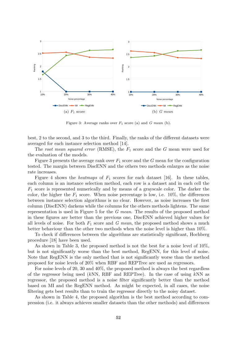
10% 20% 30% 40%1

1.5

2

2.5

3

DiscENN MI RegENN

Noise percentage

Ra

nki

ng

(a) F1 score

10% 20% 30% 40%1

1.5

2

2.5

3

DiscENN MI RegENN

Noise percentage

Ra

nki

ng

(b) G mean

Figure 3: Average ranks over F1 score (a) and G mean (b).

best, 2 to the second, and 3 to the third. Finally, the ranks of the different datasets wereaveraged for each instance selection method [14].

The root mean squared error (RMSE), the F1 score and the G mean were used forthe evaluation of the models.

Figure 3 presents the average rank over F1 score and the G mean for the configurationtested. The margin between DiscENN and the others two methods enlarges as the noiserate increases.

Figure 4 shows the heatmaps of F1 scores for each dataset [16]. In these tables,each column is an instance selection method, each row is a dataset and in each cell theF1 score is represented numerically and by means of a grayscale color. The darker thecolor, the higher the F1 score. When noise percentage is low, i.e. 10%, the differencesbetween instance selection algorithms is no clear. However, as noise increases the firstcolumn (DiscENN) darkens while the columns for the others methods lightens. The samerepresentation is used in Figure 5 for the G mean. The results of the proposed methodin these figures are better than the previous one, DiscENN achieved higher values forall levels of noise. For both F1 score and G mean, the proposed method shows a muchbetter behaviour than the other two methods when the noise level is higher than 10%.

To check if differences between the algorithms are statistically significant, Hochbergprocedure [18] have been used.

As shown in Table 3, the proposed method is not the best for a noise level of 10%,but is not significantly worse than the best method, RegENN, for this level of noise.Note that RegENN is the only method that is not significantly worse than the methodproposed for noise levels of 20% when RBF and REPTree are used as regressors.

For noise levels of 20, 30 and 40%, the proposed method is always the best regardlessof the regressor being used (kNN, RBF and REPTree). In the case of using kNN asregressor, the proposed method is a noise filter significantly better than the methodbased on MI and the RegENN method. As might be expected, in all cases, the noisefiltering gets best results than to train the regressor directly to the noisy dataset.

As shown in Table 4, the proposed algorithm is the best method according to com-pression (i.e. it always achieves smaller datasets than the other methods) and differences

52

DiscENN MI RegENN

mvhousecaliforniaelevatorspoleaileronsdelta-elvpuma32hcompactivdelta-ailabaloneANACALTquakeplasticwankarawizmirfriedmanele-2mortgagetreasuryconcretelaserstockele-1autoMPG6autoMPG8deebaseballmachineCPU

0.4025 0.3115 0.46530.4676 0.0186 0.55480.2745 0.0864 0.27300.3632 0.2163 0.54830.5836 0.4179 0.59390.3852 0.0347 0.52770.3851 0.3609 0.43750.2132 0.0387 0.02190.7272 0.0643 0.63970.4709 0.4728 0.56300.3163 0.1060 0.38380.1221 0.0151 0.02070.8636 0.0803 0.59460.1885 0.2304 0.13290.4610 0.5460 0.55260.4963 0.5651 0.53430.2774 0.3323 0.22890.1306 0.0101 0.02350.6759 0.4751 0.67030.7260 0.4736 0.69300.2412 0.2151 0.16240.5631 0.5512 0.63560.6582 0.4841 0.66160.2904 0.1637 0.39790.2944 0.3964 0.36970.2957 0.3732 0.38180.2691 0.2643 0.22240.3219 0.2551 0.41040.4658 0.1863 0.5246

(a) Noise 10%

DiscENN MI RegENN


0.5764 0.1907 0.28300.6476 0.0188 0.36390.4484 0.0565 0.17490.5419 0.1749 0.35630.7400 0.2695 0.37050.5746 0.0242 0.34090.5742 0.3628 0.26800.3681 0.0398 0.01370.7558 0.0399 0.42290.6458 0.4596 0.35390.4996 0.0548 0.25430.2141 0.0143 0.01580.8685 0.0925 0.25850.3275 0.1988 0.08050.6449 0.4759 0.36070.6859 0.4726 0.33990.4492 0.2889 0.14770.2433 0.0122 0.02160.7928 0.2940 0.44410.8330 0.2688 0.43710.4064 0.1920 0.09820.7170 0.4829 0.40810.8189 0.3225 0.37340.4738 0.1713 0.27830.4815 0.3599 0.22090.4878 0.2818 0.22610.4501 0.2412 0.14910.5059 0.2469 0.23090.6091 0.1681 0.2926

(b) Noise 20%

DiscENN MI RegENN


0.6722 0.1060 0.15580.7393 0.0195 0.19850.5669 0.0375 0.09970.6387 0.1417 0.20590.8092 0.1375 0.19280.6790 0.0185 0.19780.6766 0.3159 0.14510.4829 0.0383 0.00850.7710 0.0217 0.23500.7267 0.3903 0.19140.6140 0.0340 0.14180.3144 0.0133 0.00980.7841 0.0860 0.08060.4336 0.1363 0.04660.7349 0.3923 0.19960.7532 0.3649 0.18690.5646 0.2412 0.09440.3425 0.0243 0.01780.8430 0.1311 0.24270.8691 0.1196 0.25450.5193 0.1699 0.06160.7590 0.4016 0.22640.8573 0.2160 0.16050.5883 0.1752 0.15290.5902 0.2969 0.13030.5840 0.2275 0.12240.5524 0.1677 0.08720.6232 0.2016 0.13550.6949 0.1839 0.1617

(c) Noise 30%

DiscENN MI RegENN


0.7306 0.0589 0.07810.7936 0.0200 0.09750.6508 0.0247 0.05260.6875 0.1161 0.10850.8461 0.0582 0.08650.7465 0.0140 0.10300.7421 0.2725 0.06920.5734 0.0364 0.00450.7760 0.0102 0.12080.7660 0.3180 0.08900.6871 0.0172 0.07760.4200 0.0103 0.00460.6388 0.0750 0.01820.5129 0.0843 0.01660.7847 0.3249 0.10810.7893 0.2896 0.08890.6235 0.2125 0.05000.4348 0.0350 0.01000.8587 0.0655 0.14160.8905 0.0491 0.13220.5874 0.1397 0.03750.7754 0.3229 0.11790.8299 0.1228 0.06490.6614 0.1695 0.09070.6724 0.2338 0.05740.6632 0.1973 0.05630.5924 0.1042 0.06460.6922 0.1901 0.06980.7476 0.1800 0.0750

(d) Noise 40%

Figure 4: F1 score for each dataset. The darker the color is, the higher is the score (i.e. black colorrepresents F1 = 1 and white color F1 = 0.

53

DiscENN MI RegENN


0.7853 0.4381 0.55070.8385 0.0983 0.64300.6615 0.2152 0.40750.7690 0.3886 0.62920.8809 0.5771 0.66640.7872 0.1355 0.60120.7867 0.5690 0.53750.5211 0.1501 0.10550.8019 0.1833 0.69470.8368 0.6621 0.63930.7217 0.2500 0.49730.4058 0.1092 0.12420.9797 0.2324 0.66110.5252 0.4387 0.27630.8328 0.6714 0.61860.8422 0.6840 0.60580.6670 0.5081 0.36000.4318 0.0837 0.12690.8880 0.5877 0.71160.9208 0.5674 0.73180.6091 0.3891 0.29840.8654 0.6588 0.69330.9398 0.5778 0.70610.6907 0.3633 0.51030.6948 0.5691 0.48380.6939 0.5275 0.49500.6624 0.4366 0.36160.7291 0.4559 0.52140.8115 0.3888 0.6446

(a) Noise 10%

DiscENN MI RegENN


0.7814 0.3256 0.40600.8366 0.0981 0.47490.6577 0.1712 0.31130.7606 0.3212 0.46770.8813 0.4052 0.47980.7883 0.1113 0.45370.7878 0.5017 0.39450.5143 0.1463 0.08320.7966 0.1429 0.51930.8325 0.5750 0.46520.7202 0.1703 0.38340.4329 0.0938 0.09450.9481 0.2308 0.38660.5159 0.3606 0.20820.8333 0.5739 0.46990.8495 0.5711 0.45350.6591 0.4300 0.28300.4644 0.0857 0.11180.8916 0.4201 0.53480.9211 0.3956 0.53060.6071 0.3425 0.22770.8620 0.5753 0.50810.9390 0.4433 0.48060.6920 0.3312 0.40580.7032 0.4908 0.35450.7106 0.4171 0.35840.6724 0.3824 0.28540.7301 0.4004 0.36640.7937 0.3294 0.4287

(b) Noise 20%

DiscENN MI RegENN


0.7761 0.2368 0.29060.8321 0.0997 0.33240.6516 0.1384 0.22940.7443 0.2802 0.33900.8786 0.2732 0.32710.7820 0.0968 0.33140.7787 0.4437 0.27990.5037 0.1412 0.06550.8013 0.1048 0.36510.8205 0.5010 0.32550.7134 0.1322 0.27650.4418 0.0854 0.07130.8593 0.2157 0.20530.4999 0.2789 0.15520.8272 0.4986 0.33330.8371 0.4768 0.32140.6582 0.3785 0.22290.4768 0.1162 0.09730.8918 0.2655 0.37220.9116 0.2528 0.38250.5924 0.3123 0.17890.8362 0.5055 0.35790.9208 0.3504 0.29580.6841 0.3206 0.28870.6930 0.4259 0.26550.6906 0.3632 0.25630.6696 0.3058 0.21420.7283 0.3443 0.27030.7923 0.3299 0.3001

(c) Noise 30%

DiscENN MI RegENN


0.7673 0.1743 0.20150.8254 0.1006 0.22650.6418 0.1118 0.16440.7146 0.2495 0.23960.8735 0.1733 0.21270.7747 0.0839 0.23310.7683 0.4004 0.18940.4926 0.1367 0.04730.8007 0.0716 0.25360.8000 0.4372 0.21590.6991 0.0932 0.20110.4175 0.0729 0.04800.6873 0.1984 0.09580.4706 0.2121 0.09160.8186 0.4420 0.23910.8244 0.4128 0.21580.6400 0.3475 0.16030.4752 0.1358 0.07160.8822 0.1841 0.27640.9096 0.1587 0.26660.5705 0.2768 0.13850.8144 0.4400 0.25050.8591 0.2573 0.18340.6653 0.3085 0.21840.6862 0.3680 0.17270.6814 0.3324 0.17060.6422 0.2360 0.18320.7146 0.3279 0.19070.7872 0.3192 0.1995

(d) Noise 40%

Figure 5: G mean for each dataset. The darker the color is, the higher is the score (i.e. black colorrepresents G = 1 and white color G = 0.

54

Table 3: Average ranks and Hochberg procedure over RMSE. The 6 means that the result of thealgorithm is significantly worse than the best (the first of the ranking is highlighted in bold) at aconfidence level of 0.95, we included NoFilter that shows the performance of the regressor trained overnoisy datasets.

kNN

IS Alg.% noise

10 20 30 40

DiscENN 2.172 1.465 1.172 1.207MI 2.534 2.638 6 2.207 6 2.086 6RegENN 1.776 2.224 6 3.965 6 3.965 6NoFilter 3.517 6 3.672 6 2.655 6 2.741 6

RBF

IS Alg.% noise

10 20 30 40

DiscENN 2.327 1.672 1.431 1.465MI 2.483 2.603 6 2.707 6 2.758 6RegENN 1.983 2.121 2.327 6 2.379 6NoFilter 3.207 6 3.603 6 3.534 6 3.396 6

REPTree

IS Alg.% noise

10 20 30 40

DiscENN 2.172 1.638 1.431 1.396MI 2.621 2.862 6 2.810 6 2.931 6RegENN 2.000 2.034 2.172 6 2.293 6NoFilter 3.207 6 3.465 6 3.586 6 3.379 6

55

Table 4: Average ranks and Hochberg procedure over compression. The 6 means that the result of thealgorithm is worse than the best (the first of the ranking is highlighted in bold) at a confidence level of0.95.

IS Alg.% noise

10 20 30 40

DiscENN 1.000 1.000 1.000 1.000MI 2.414 6 2.414 6 2.345 6 2.345 6RegENN 2.586 6 2.586 6 2.655 6 2.655 6

are significant at a confidence level of 0.95.Finally, with the aim to evaluate how well the instance selection works, average

ranks over the three regressors were made. Table 5 shows the average ranks, the dashedline indicates that the difference between the first method and the others below theline is significant at a confidence level of 0.95. The table provides an indication ofthe performance of the different methods with different levels of noise: 10, 20, 30 and40%. For all noise levels, the lowest error is achieved by RBF. When the noise levelis only 10%, the selection done by RegENN outperforms the one done by DiscENN.However, as the noise level increases, the performance of the proposed method pays off,and the selection achieved by this method gives better results than the others. Whenthe noise level is only 10%, the selection done by RegENN outperforms the one done byDiscENN. Also note that for noise levels of 30% and 40% the proposed method improvesthe results for all base regressor. As might be expected, kNN is the worst regressorin noisy environments, so it ranks low in all cases, however it is very noticeable thatits rank improves remarkably when it is trained with the selection performed by theproposed method. This improvement is achieved even in the cases with high noise levels(30% and 40%), up to the point that it ranks second. Thus, the algorithm proposed inthis paper allows to use regressors, which are not able to deal well with noise, in noisyenvironments.

5. Conclusions and future work

The construction of expert and intelligent systems requires the elicitation of theknowledge that they are going to use. Although in the past this required the inter-vention of experts in the subject matter of automation, today with the abundance ofdata, it is most frequent to obtain knowledge using data mining algorithms. However,there are two circumstances that may affect the use of these algorithms. On the onehand, some are very sensitive to noise. On the other hand, the presence of noise in theprocess of obtaining data is almost inevitable (for example, measurements in industrialenvironments).

Although there are numerous algorithms for instance selection in classification (thevalue to predict is discrete), it does not happen the same for problems in which thevalue to predict is continuous. The main contribution of this paper is a new approachto the problem of instance selection in regression. The approach is simple, even naive,the output variable is discretized to make use of an instance selection algorithm forclassification. Besides simplicity, another major advantage of the method is that we now

56

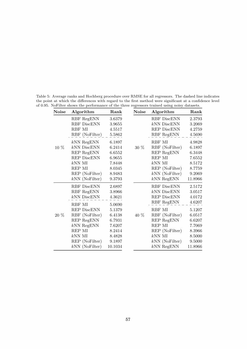
Table 5: Average ranks and Hochberg procedure over RMSE for all regressors. The dashed line indicatesthe point at which the differences with regard to the first method were significant at a confidence levelof 0.95. NoFilter shows the performance of the three regressors trained using noisy datasets.

Noise Algorithm Rank

10 %

RBF RegENN 3.6379RBF DiscENN 3.9655RBF MI 4.5517RBF (NoFilter) 5.5862

kNN RegENN 6.1897kNN DiscENN 6.2414REP RegENN 6.6552REP DiscENN 6.9655kNN MI 7.8448REP MI 8.0345REP (NoFilter) 8.9483kNN (NoFilter) 9.3793

20 %

RBF DiscENN 2.6897RBF RegENN 3.8966kNN DiscENN 4.3621

RBF MI 5.0690REP DiscENN 5.1379RBF (NoFilter) 6.4138REP RegENN 6.7931kNN RegENN 7.6207REP MI 8.2414kNN MI 8.4828REP (NoFilter) 9.1897kNN (NoFilter) 10.1034

Noise Algorithm Rank

30 %

RBF DiscENN 2.3793kNN DiscENN 3.2069REP DiscENN 4.2759RBF RegENN 4.5690

RBF MI 4.9828RBF (NoFilter) 6.1897REP RegENN 6.3448REP MI 7.6552kNN MI 8.5172REP (NoFilter) 8.7759kNN (NoFilter) 9.2069kNN RegENN 11.8966

40 %

RBF DiscENN 2.5172kNN DiscENN 3.0517REP DiscENN 4.0172RBF RegENN 4.6207

RBF MI 5.1207RBF (NoFilter) 6.0517REP RegENN 6.6207REP MI 7.7069REP (NoFilter) 8.3966kNN MI 8.5000kNN (NoFilter) 9.5000kNN RegENN 11.8966

57

have at our disposal all the algorithms of instance selection for classification existingin the literature. The utility of the approach has been proved experimentally, it offerscompetitive results when compare to the few existing methods of instance selection fornoise removal in regression [23, 35], despite that the latter propose a more complex andsophisticated approaches to the problem. More specifically, its performance as a noisefilter has been compared i) taking as reference the values of: the RMSE, the F1 score, theG mean and the compression; ii) with different base regressors: k-nearest neighbours,RBF networks and REPTree, and iii) using 29 data set to which several levels of noisewere added.

The main criticism that can be made to the proposal is the lack of theoretical justifica-tion. But the idea to address a continuous problem by means of a previous discretizationstep is a classical approach, perhaps the most representative example are the Rienmannsums to approximate the area under a curve and solve the problem of numerical integra-tion. In any case, the discretization that is being done at the current implementation istoo crude. We suspect that a discretization step more adjusted to the specific nature ofthe data could improve the method. The combination of results obtained with differentdiscretizations could be beneficial as well (following a similar approach to the one used byensemble methods). It may also be interesting to investigate whether the way in whichthe discretization is done affects the performance of the proposed approach. We hope toincorporate all these ideas in future research.

Another preprocessing operation that helps in the design of expert and intelligentsystems is the selection of features [54, 7]. Some authors have successfully adapted tofeature selection ideas originally designed for instance selection [26]. This makes us thinkthat we too could do the same with our idea. In classification, simultaneous selection ofinstances and features has also proved to be beneficial [15], so perhaps our method canbe also extended to this simultaneous selection. Finally, although our method has showngood results in a large set of standard datasets for benchmarking, it would be interestingto check its performance on specific domains, especially in industrial problems and intime series forecasting.

Acknowledgments

This work was supported by the project TIN2011-24046 of the Spanish Ministry ofEconomy and Competitiveness.

References

[1] Aha, D., Kibler, D., & Albert, M. (1991). Instance-based learning algorithms. Machine Learning,6 , 37–66. doi:10.1007/BF00153759.

[2] Ahn, H., & Kim, K. (2009). Bankruptcy prediction modeling with hybrid case-based reasoning andgenetic algorithms approach. Applied Soft Computing, 9 , 599 – 607. doi:10.1016/j.asoc.2008.08.002.

[3] Alcala, R., Alcala-Fdez, J., Herrera, F., & Otero, J. (2007). Genetic learning of accurate andcompact fuzzy rule based systems based on the 2-tuples linguistic representation. InternationalJournal of Approximate Reasoning, 44 , 45 – 64. doi:10.1016/j.ijar.2006.02.007. Genetic FuzzySystems and the Interpretability-Accuracy Trade-off.

[4] Alcala-Fdez, J., Fernandez, A., Luengo, J., Derrac, J., & Garcıa, S. (2011). Keel data-miningsoftware tool: Data set repository, integration of algorithms and experimental analysis framework.Multiple-Valued Logic and Soft Computing, 17 , 255–287.

58

[5] Antonelli, M., Ducange, P., & Marcelloni, F. (2012). Genetic training instance selection in multiob-jective evolutionary fuzzy systems: A coevolutionary approach. Fuzzy Systems, IEEE Transactionson, 20 , 276–290. doi:10.1109/TFUZZ.2011.2173582.

[6] Barandela, R., Ferri, F. J., & Sanchez, J. S. (2005). Decision boundary preserving prototypeselection for nearest neighbor classification. International Journal of Pattern Recognition andArtificial Intelligence, 19 , 787–806. doi:10.1142/S0218001405004332.

[7] Bennasar, M., Hicks, Y., & Setchi, R. (2015). Feature selection using joint mutual informationmaximisation. Expert Systems with Applications, 42 , 8520 – 8532. doi:10.1016/j.eswa.2015.07.007.

[8] Blachnik, M., & Kordos, M. (2014). Bagging of instance selection algorithms. In L. Rutkowski,M. Korytkowski, R. Scherer, R. Tadeusiewicz, L. A. Zadeh, & J. M. Zurada (Eds.), ArtificialIntelligence and Soft Computing (pp. 40–51). Springer International Publishing volume 8468 ofLecture Notes in Computer Science. doi:10.1007/978-3-319-07176-3_4.

[9] Bootkrajang, J., & Kaban, A. (2014). Learning kernel logistic regression in the presence of classlabel noise. Pattern Recognition, 47 , 3641 – 3655. doi:10.1016/j.patcog.2014.05.007.

[10] Brighton, H., & Mellish, C. (2002). Advances in instance selection for instance-based learningalgorithms. Data Mining and Knowledge Discovery, 6 , 153–172. doi:10.1023/A:1014043630878.

[11] Buza, K., Nanopoulos, A., & Schmidt-Thieme, L. (2011). INSIGHT: Efficient and effective instanceselection for time-series classification. In J. Huang, L. Cao, & J. Srivastava (Eds.), Advances inKnowledge Discovery and Data Mining (pp. 149–160). Springer Berlin Heidelberg volume 6635 ofLecture Notes in Computer Science. doi:10.1007/978-3-642-20847-8_13.

[12] Cavalcanti, G. D., Ren, T. I., & Pereira, C. L. (2013). ATISA: Adaptive threshold-based instanceselection algorithm. Expert Systems with Applications, 40 , 6894 – 6900. doi:10.1016/j.eswa.2013.06.053.

[13] Chen, Z.-Y., Lin, W.-C., Ke, S.-W., & Tsai, C.-F. (2015). Evolutionary feature and instanceselection for traffic sign recognition. Computers in Industry, 74 , 201 – 211. doi:10.1016/j.compind.2015.08.007.

[14] Demsar, J. (2006). Statistical comparisons of classifiers over multiple data sets. J. Mach. Learn.Res., 7 , 1–30. URL: http://dl.acm.org/citation.cfm?id=1248547.1248548.

[15] Derrac, J., Garcıa, S., & Herrera, F. (2010). IFS-CoCo: Instance and feature selection basedon cooperative coevolution with nearest neighbor rule. Pattern Recognition, 43 , 2082 – 2105.doi:10.1016/j.patcog.2009.12.012.

[16] Garcia, L. P., de Carvalho, A. C., & Lorena, A. C. (2015). Effect of label noise in the complexityof classification problems. Neurocomputing, 160 , 108 – 119. doi:10.1016/j.neucom.2014.10.085.

[17] Garcıa, S., Derrac, J., Cano, J., & Herrera, F. (2012). Prototype selection for nearest neighborclassification: Taxonomy and empirical study. Pattern Analysis and Machine Intelligence, IEEETransactions on, 34 , 417–435. doi:10.1109/TPAMI.2011.142.

[18] Garcıa, S., Fernandez, A., Luengo, J., & Herrera, F. (2010). Advanced nonparametric tests formultiple comparisons in the design of experiments in computational intelligence and data mining:Experimental analysis of power. Inf. Sci., 180 , 2044–2064. doi:10.1016/j.ins.2009.12.010.

[19] Garcıa, V., Marques, A., & Sanchez, J. (2012). On the use of data filtering techniques for creditrisk prediction with instance-based models. Expert Systems with Applications, 39 , 13267 – 13276.doi:10.1016/j.eswa.2012.05.075.

[20] Garcıa-Osorio, C., de Haro-Garcıa, A., & Garcıa-Pedrajas, N. (2010). Democratic instance selection:A linear complexity instance selection algorithm based on classifier ensemble concepts. ArtificialIntelligence, 174 , 410 – 441. doi:10.1016/j.artint.2010.01.001.

[21] Garcıa-Pedrajas, N., & de Haro-Garcıa, A. (2014). Boosting instance selection algorithms.Knowledge-Based Systems, 67 , 342 – 360. doi:10.1016/j.knosys.2014.04.021.

[22] Garcıa-Pedrajas, N., Perez-Rodrıguez, J., Garcıa-Pedrajas, M. D., Ortiz-Boyer, D., & Fyfe, C.(2012). Class imbalance methods for translation initiation site recognition in DNA sequences.Knowledge-Based Systems, 25 , 22 – 34. doi:10.1016/j.knosys.2011.05.002. Special Issue on NewTrends in Data Mining.

[23] Guillen, A., Herrera, L., Rubio, G., Pomares, H., Lendasse, A., & Rojas, I. (2010). New method forinstance or prototype selection using mutual information in time series prediction. Neurocomputing,73 , 2030 – 2038. doi:10.1016/j.neucom.2009.11.031. Subspace Learning / Selected papers fromthe European Symposium on Time Series Prediction.

[24] Hall, M., Frank, E., Holmes, G., Pfahringer, B., Reutemann, P., & Witten, I. H. (2009). The wekadata mining software: An update. SIGKDD Explorations, .

[25] Harding, J. A., Shahbaz, M., Srinivas, & Kusiak, A. (2005). Data mining in manufacturing: a review.

59

Journal of Manufacturing Science and Engineering, 128 , 969–976. doi:10.1115/1.2194554.[26] de Haro-Garcıa, A., & Garcıa-Pedrajas, N. (2010). Scaling up feature selection by means of de-

mocratization. In N. Garcıa-Pedrajas, F. Herrera, C. Fyfe, J. M. Benıtez, & M. Ali (Eds.), Trendsin Applied Intelligent Systems (pp. 662–672). Springer Berlin Heidelberg volume 6097 of LectureNotes in Computer Science. doi:10.1007/978-3-642-13025-0_68.

[27] Hart, P. (1968). The condensed nearest neighbor rule (corresp.). Information Theory, IEEETransactions on, 14 , 515 – 516. doi:10.1109/TIT.1968.1054155.

[28] Herrera, F. (2008). Genetic fuzzy systems: taxonomy, current research trends and prospects.Evolutionary Intelligence, 1 , 27–46. doi:10.1007/s12065-007-0001-5.

[29] Herrera, L. J., Pomares, H., Rojas, I., Verleysen, M., & Guilen, A. (2006). Effective input variableselection for function approximation. In S. D. Kollias, A. Stafylopatis, W. Duch, & E. Oja (Eds.),Artificial Neural Networks - ICANN 2006 (pp. 41–50). Springer Berlin Heidelberg volume 4131 ofLecture Notes in Computer Science. doi:10.1007/11840817_5.

[30] Jankowski, N., & Grochowski, M. (2004). Comparison of instances seletion algorithms I. algorithmssurvey. In L. Rutkowski, J. Siekmann, R. Tadeusiewicz, & L. Zadeh (Eds.), Artificial Intelligenceand Soft Computing - ICAISC 2004 (pp. 598–603). Springer Berlin Heidelberg volume 3070 ofLecture Notes in Computer Science. doi:10.1007/978-3-540-24844-6_90.

[31] Keogh, E., & Kasetty, S. (2002). On the need for time series data mining benchmarks: a surveyand empirical demonstration. In Proceedings of the eighth ACM SIGKDD international conferenceon Knowledge discovery and data mining KDD ’02 (pp. 102–111). New York, NY, USA: ACM.doi:10.1145/775047.775062.

[32] Kim, K.-J. (2006). Artificial neural networks with evolutionary instance selection for financialforecasting. Expert Systems with Applications, 30 , 519 – 526. doi:10.1016/j.eswa.2005.10.007.Intelligent Information Systems for Financial Engineering.

[33] Kononenko, I., & Kukar, M. (2007). Machine Learning and Data Mining: Introduction to Principlesand Algorithms. Horwood Publishing Limited.

[34] Kordos, M., Bia lka, S., & Blachnik, M. (2013). Instance selection in logical rule extraction forregression problems. In L. Rutkowski, M. Korytkowski, R. Scherer, R. Tadeusiewicz, L. Zadeh,& J. Zurada (Eds.), Artificial Intelligence and Soft Computing (pp. 167–175). Springer BerlinHeidelberg volume 7895 of Lecture Notes in Computer Science. doi:10.1007/978-3-642-38610-7_16.

[35] Kordos, M., & Blachnik, M. (2012). Instance selection with neural networks for regression problems.In Proceedings of the 22nd international conference on Artificial Neural Networks and MachineLearning - Volume Part II ICANN’12 (pp. 263–270). Berlin, Heidelberg: Springer-Verlag. doi:10.1007/978-3-642-33266-1_33.

[36] Koskima aki, H., Juutilainen, I., Laurinen, P., & Roning, J. (2008). Two-level clustering approachto training data instance selection: A case study for the steel industry. In Neural Networks, 2008.IJCNN 2008. (IEEE World Congress on Computational Intelligence). IEEE International JointConference on (pp. 3044–3049). doi:10.1109/IJCNN.2008.4634228.

[37] Kwak, N., & Lee, J.-W. (2010). Feature extraction based on subspace methods for regression prob-lems. Neurocomputing, 73 , 1740 – 1751. doi:10.1016/j.neucom.2009.10.025. Subspace Learning/ Selected papers from the European Symposium on Time Series Prediction.

[38] Lei, J. Z., & Ghorbani, A. A. (2012). Improved competitive learning neural networks for networkintrusion and fraud detection. Neurocomputing, 75 , 135 – 145. doi:10.1016/j.neucom.2011.02.021. Brazilian Symposium on Neural Networks (SBRN 2010) International Conference on HybridArtificial Intelligence Systems (HAIS 2010).

[39] Lewis, D. D., & Gale, W. A. (1994). A sequential algorithm for training text classifiers. In Pro-ceedings of the 17th Annual International ACM SIGIR Conference on Research and Developmentin Information Retrieval SIGIR ’94 (pp. 3–12). New York, NY, USA: Springer-Verlag New York,Inc. doi:10.1007/978-1-4471-2099-5_1.

[40] Leyva, E., Gonzalez, A., & Perez, R. (2015). Three new instance selection methods based onlocal sets: A comparative study with several approaches from a bi-objective perspective. PatternRecognition, 48 , 1523 – 1537. doi:10.1016/j.patcog.2014.10.001.

[41] Liu, D., Yamashita, Y., & Ogawa, H. (1995). Pattern recognition in the presence of noise. PatternRecognition, 28 , 989 – 995. doi:10.1016/0031-3203(94)00174-K.

[42] Marchiori, E. (2010). Class conditional nearest neighbor for large margin instance selection. PatternAnalysis and Machine Intelligence, IEEE Transactions on, 32 , 364–370. doi:10.1109/TPAMI.2009.164.

[43] Nanni, L., & Lumini, A. (2011). Prototype reduction techniques: A comparison among different

60

approaches. Expert Systems with Applications, 38 , 11820 – 11828. doi:10.1016/j.eswa.2011.03.070.

[44] Rodriguez-Fdez, I., Mucientes, M., & Bugarin, A. (2013). An instance selection algorithm for regres-sion and its application in variance reduction. In Fuzzy Systems (FUZZ), 2013 IEEE InternationalConference on (pp. 1–8). doi:10.1109/FUZZ-IEEE.2013.6622486.

[45] Rui, Y., Huang, T. S., & Chang, S.-F. (1999). Image retrieval: Current techniques, promisingdirections, and open issues. Journal of Visual Communication and Image Representation, 10 , 39– 62. doi:10.1006/jvci.1999.0413.

[46] Saez, J. A., Luengo, J., & Herrera, F. (2013). Predicting noise filtering efficacy with data complexitymeasures for nearest neighbor classification. Pattern Recognition, 46 , 355 – 364. doi:10.1016/j.patcog.2012.07.009.

[47] Sanchez, J. S., Pla, F., & Ferri, F. J. (1997). Prototype selection for the nearest neighbour rulethrough proximity graphs. Pattern Recognition Letters, 18 , 507 – 513. doi:10.1016/S0167-8655(97)00035-4.

[48] Santos, J. C. R., Aguilar-Ruiz, J. S., & Toro, M. (2003). Finding representative patterns withordered projections. Pattern Recognition, 36 , 1009–1018. doi:10.1016/S0031-3203(02)00119-X.

[49] Serrano, E., Gomez-Sanz, J. J., Botıa, J. A., & Pavon, J. (2009). Intelligent data analysis applied todebug complex software systems. Neurocomputing, 72 , 2785 – 2795. doi:10.1016/j.neucom.2008.10.025. Hybrid Learning Machines (HAIS 2007) / Recent Developments in Natural Computation(ICNC 2007).

[50] Stojanovic, M. B., Bozic, M. M., Stankovic, M. M., & Stajic, Z. P. (2014). A methodology fortraining set instance selection using mutual information in time series prediction. Neurocomputing,141 , 236 – 245. doi:10.1016/j.neucom.2014.03.006.

[51] Sun, J., & Li, H. (2011). Dynamic financial distress prediction using instance selection for thedisposal of concept drift. Expert Systems with Applications, 38 , 2566 – 2576. doi:10.1016/j.eswa.2010.08.046.

[52] Tolvi, J. (2004). Genetic algorithms for outlier detection and variable selection in linear regressionmodels. Soft Comput., 8 , 527–533. doi:10.1007/s00500-003-0310-2.

[53] Trentin, E., & Gori, M. (2001). A survey of hybrid ANN/HMM models for automatic speechrecognition. Neurocomputing, 37 , 91–126. doi:10.1016/S0925-2312(00)00308-8.

[54] Uysal, A. K. (2016). An improved global feature selection scheme for text classification. ExpertSystems with Applications, 43 , 82 – 92. doi:10.1016/j.eswa.2015.08.050.

[55] Van Rijsbergen, C. (1979). Information Retrieval . Butterworth.[56] Wang, L., Huang, Y., Luo, X., Wang, Z., & Luo, S. (2011). Image deblurring with filters learned by

extreme learning machine. Neurocomputing, 74 , 2464 – 2474. doi:10.1016/j.neucom.2010.12.035.Advances in Extreme Learning Machine: Theory and Applications Biological Inspired Systems.Computational and Ambient Intelligence Selected papers of the 10th International Work-Conferenceon Artificial Neural Networks (IWANN2009).

[57] Wilson, D. L. (1972). Asymptotic properties of nearest neighbor rules using edited data. Systems,Man and Cybernetics, IEEE Transactions on, SMC-2 , 408–421. doi:10.1109/TSMC.1972.4309137.

[58] Wilson, D. R., & Martinez, T. R. (2000). Reduction techniques for instance-based learning algo-rithms. Machine Learning, 38 , 257–286. doi:10.1023/A:1007626913721.

[59] Witten, I., & Frank, E. (2005). Data mining: practical machine learning tools and techniques.Morgan Kaufmann series in data management systems. Morgan Kaufman.

[60] Wu, X., & Zhu, X. (2008). Mining with noise knowledge: Error-aware data mining. Systems, Manand Cybernetics, Part A: Systems and Humans, IEEE Transactions on, 38 , 917–932. doi:10.1109/TSMCA.2008.923034.

[61] Zhu, X., & Wu, X. (2004). Class noise vs. attribute noise: A quantitative study. Artificial Intelli-gence Review , 22 , 177–210. doi:10.1007/s10462-004-0751-8.

61

If we had access to a classifier with perfectgeneralization performance, there wouldbe no need to resort to ensembletechniques.

Polikar (2006) CH

AP

TE

R

2FUSION OF INSTANCE SELECTION METHODS IN REGRESSION TASKS

This journal paper presents the advantages of using a combination of instance selection

methods in regression. The combination of multiple learners into an ensemble that has

greater power than the sum of any one of its members is nothing new in itself. However,

combinations of instance selection methods applied to regression tasks is a novel aspect that has

not previously been tested.

Four instance selection methods, two edition algorithms and two condensation algorithms,

were combined in homogeneous ensembles. Their superior performance supported the underlying

principle of general ensembles: they work better than each method by itself alone

Authors: Álvar Arnaiz-González, Marcin Blachnik, Mirosław Kordos, César García-Osorio

Type: Journal

Published in: Information Fusion 30: 69 – 79

Year: 2016

Reference: Arnaiz-González et al. (2016)

63

Fusion of Instance Selection Methods in Regression TasksI

Alvar Arnaiz-Gonzaleza, Marcin Blachnikb, Miros law Kordosc, Cesar Garcıa-Osorioa

aUniversity of Burgos, SpainbSilesian University of Technology, Poland

cUniversity of Bielsko-Biala, Poland

Abstract

Data pre-processing is a very important aspect of data mining. In this paper we discussinstance selection used for prediction algorithms, which is one of the pre-processing ap-proaches. The purpose of instance selection is to improve the data quality by data sizereduction and noise elimination.

Until recently, instance selection has been applied mainly to classification problems.Very few recent papers address instance selection for regression tasks.

This paper proposes fusion of instance selection algorithms for regression tasks toimprove the selection performance. As the members of the ensemble two different familiesof instance selection methods are evaluated: one based on distance threshold and theother one on converting the regression task into a multiple class classification task.

Extensive experimental evaluation performed on the two regression versions of theEdited Nearest Neighbor (ENN) and Condensed Nearest Neighbor (CNN) methods showedthat the best performance measured by the error value and data size reduction are inmost cases obtained for the ensemble methods.

Keywords: instance selection, regression, ensemble models

1. Introduction

In real-world problems, we are often faced with regression tasks, aimed at predictingsome real-value numbers. The quality of the prediction is often limited not by

the learning algorithm, but by the quality of the data itself. There are various waysof improving the quality of the data on which the learning model is built. One of them isinstance selection, in which we reject the training instances that are either not expectedto improve or are expected to worsen prediction results.

In this paper, we use ‘edited’ or ‘filtered’ dataset interchangeably to refer to a datasetproduced by an instance selection process.

Traditionally, instance selection methods are divided in two groups according to theapproach used by algorithms to select an instance [29]:

IThis work was supported by the Project TIN2011-24046 of the Spanish Ministry of Economy andCompetitiveness.

Email addresses: [email protected] (Alvar Arnaiz-Gonzalez), [email protected] (MarcinBlachnik), [email protected] (Miros law Kordos), [email protected] (Cesar Garcıa-Osorio)

Preprint submitted to Information Fusion November 10, 2017

64

• Wrappers: the algorithms of this family use the accuracy obtained by the classifier(usually the same that will be used after instance selection stage). Some of themare CNN [17], ENN [41], DROP1. . . 5 [40], ICF [8], MSS [4]. . .

• Filters: as opposed to wrappers, the instance selection or rejection criterion is notbased on a classifier. For example POP [32].

A large number of instance selection algorithms designed for classification tasks havebeen published in the scientific literature and new ones continue to appear. An up-to-datetaxonomy can be found in [13].

However, two issues still require prompt attention: extending instance selectionmethodologies into regression tasks and applying the fusion of various sources to ob-tain better results. Regarding the first issue, we have already obtained some resultsin [21] and in this paper we propose a new approach based on the discretization of theoutput variable. The second issue has proven to be an effective approach in other do-mains [24], but to the best of our knowledge, no one has yet tried to apply ensembles tothe combination of instance selection methods for regression.

The presence of noise is a common problem in Data Mining applications and noisefilters are widely used to cope with this problem [35]. The usefulness and efficiency ofinstance selection methods for low quality and noisy data was confirmed in [23], whichpresented an experimental evaluation of several approaches to noise-resistant training ofmultilayer perceptron neural networks for classification and regression problems. Differ-ent noise reduction methods were evaluated with different noise levels in the data. Forregression tasks, in most cases the solution that used the threshold-based ENN instanceselection (in the following sections, we describe threshold-based ENN, short of EditedNearest Neighbor, in detail) achieved the lowest mean-square error (MSE) on the test setfor various levels of noise added to the data. The only exception was when the noise levelwas extremely high and for that case the lowest MSE was obtained by a combination ofthe threshold-based ENN with modification of the error function.

This paper is structured as follows: Section 2 is a brief review of instance selectionmethods for classification; Section 3 explains the problems of applying them to regres-sion tasks; Subsection 3.1 presents the threshold-based approach, while Subsection 3.2suggests another idea based on numerical target discretization; Section 4 shows the pos-sibility of applying the idea of ensembles to the instance selection paradigm. Then, inSection 5 an experimental study is performed to compare both approaches and the im-provements achieved when they are used within an ensemble, and how, in this case, wecan outperform the regressor trained with the whole dataset. Finally, Section 6 sum-marizes the most important conclusions, and Section 7 presents some future lines ofresearch.

2. Instance Selection for Classification

In general, instance selection algorithms can be classified into three types: noise filters,condensation algorithms and prototype selection algorithms [19]. Noise filters removeinstances that show extreme differences with their neighbors, as they are considerednoise. In the Edited Nearest Neighbor (ENN) algorithm [41] used for classification tasks,an instance is removed if it belongs to a different class than that predicted by the k

65

Nearest Neighbors algorithm (kNN), using the k nearest neighbors of the instance ofinterest. The condensation methods serve to reduce the number of instances in thedataset by removing instances that are overly similar to their neighbors. The CondensedNearest Neighbor algorithm (CNN) [17] removes the instances in classification problemsthat are correctly predicted by kNN, as it is assumed that they do not bring any newinformation to build the classifier. Prototype selection methods do not select relevantinstances, but rather transform the whole dataset into a few instances, each covering anarea corresponding to the Voronoi cell1 defined by each instance. An example of suchmethods is Learning Vectors Quantization (LVQ) [20].

The decisions about instance selection or rejection are very straightforward in instanceselection for classification problems. They are based on the classification results obtainedwith an algorithm that is almost always kNN. The instance can either belong to the sameclass or to another that is different from the majority of its neighbors. The differencebetween the predicted and the real class of the instance determines the decision on itsacceptance/rejection.

3. Instance Selection for Regression

There are very few papers that address the problem of instance selection for regression.The proposed methods fall into two categories: evolutionary-based and nearest neighbor-based (which includes our methods). The evolutionary based methods have very highcomputational cost, about 3 to 4 order of magnitude higher than the nearest neighbor-based methods for medium size datasets (according to the experiments and the datareported in [2]). For bigger datasets the difference is even larger, what makes the methodsimpractical in many applications.

However, we did not find in a literature any work on instance selection for regressiontasks in a general setting, where the authors reported the improvements in terms ofcompression rate and classification accuracy even for a single arbitrary point, not tomention even the Pareto front, which we have examined in our work, so we were not ableto use those methods for comparison.

Tolvi [39] presented the use of genetic algorithms for outlier detection. That approachdoes not rely on the dataset properties and purpose, so it can be used both for classifica-tion and regression problems. However they presented the results of only two very smalldatasets (35 instances with 2 features and 21 instances with 3 features).

In [2] Antoneli et al. also presented a genetic approach using quite complex multiob-jective evolutionary algorithms with up to 300,000 evaluations of the fitness function.

In [15] Guillen et al. presented the use of mutual information for instance selectionin time series prediction. Their idea was similar to k-NN based prediction, thus theydetermined the nearest neighbors of a given point and then instead of using k-NN topredict the output value, they calculated the mutual information (MI) between thatpoint and each of their neighbors. Then they considered the loss of MI with respect toits neighbors in so that if the loss was similar to the vectors near the examined vector, this

1A Voronoi diagram (also known as Thiessen polygons or Dirichlet tessellation) is a geometricalconstruction to partition the Euclidean space. It divides the space into several polygons, Voronoi cells,each of them associated with a point, the seed. Each Voronoi cell defines a region of the space closer toits seed than to any other point, that is, the division is made according to the nearest neighbor rule [3].

66

vector was included in the filtered dataset. They evaluated their methods on artificiallygenerated data with one and two input features. Later on, Stojanovic et. al [37] extendedthe previous idea to instance selection in time series prediction.

In [33] a Class Conditional Instance Selection for Regression (CCISR) is proposed.The method is based on CCIS for classification [27]. CCIS builds two graphs: one forthe nearest neighbors of the same class as a given instance and another for other classinstances. Then a scoring function based on the distances in graphs is used to evaluate theinstances. In the regression version (CCISR), instead of using only the nearest instancesto construct these graphs, the neighborhood is defined based on the probability densityfunction of the examples. The authors provided results on several real-world datasets forfuzzy rule based systems in terms of MSE and the number of extracted rules.

In the following subsections, we present our approaches two instance selection forregression.

3.1. Threshold-based Instance Selection for Regression

Instance selection methods developed for classification are based on the analysis ofclass labels of neighbor instances to determine the rejection/acceptance of a test instance.It usually takes the form of if statements where the condition of the if statement com-pares labels of the actual test instance with its neighbors. In the case of regression, labelcomparison is not possible since output values are not nominal but continuous. Thus,rather than labels, another quantity must be compared. An intuitive approach proposedin [21] is to use a similarity-based error measure such as:

Error = |Yreal − Ypredicted| (1)

and to compare the error to the predefined threshold, to determine whether the instanceshould be accepted or rejected:

if (Error > θ) then . . . . (2)

where (. . . ), as the consequence of the if, can denote either instance acceptance or re-jection, depending on a given algorithm. To improve the performance of this method,the threshold can depend on the local properties of the dataset. When the standarddeviation of the adjacent cases (to the test case) is high, the condition should be lesssensitive to the value of error shown in Equation (1). In other cases, when the localstandard deviation is small, the condition should be more sensitive. This leads to thefollowing modification of the previous formula:

if(Error > α·std(k)

)then . . . (3)

where std(k) is the standard deviation of the outputs of the k-nearest neighbors of theinstance.

This approach was used to adapt the ENN [41] and CNN [17] algorithms to meet theregression requirements. Moreover, it can also be easily introduced into other instanceselection algorithms.

The pseudo-code of threshold-based regression ENN (T-ENN) is shown in Algo-rithm 1. It starts by iterating over the instances of the training set and in each iterationone instance xi is examined, so it is temporally removed from the training set. Then, the

67

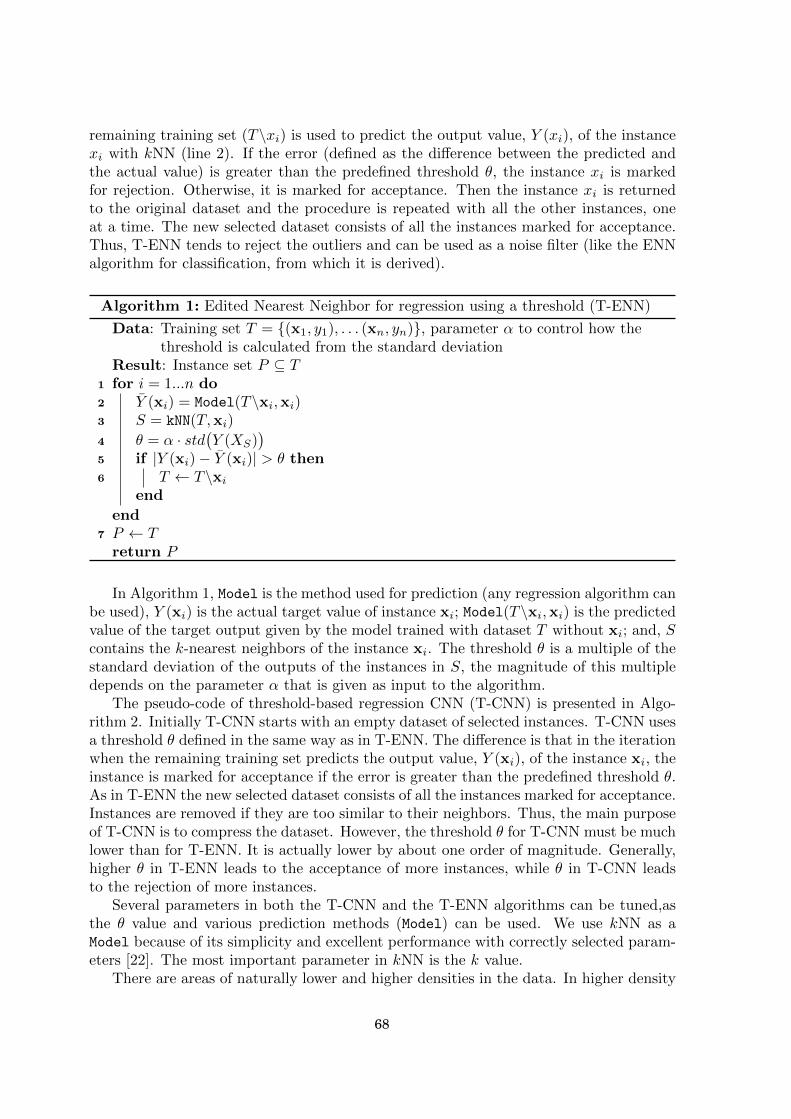
remaining training set (T\xi) is used to predict the output value, Y (xi), of the instancexi with kNN (line 2). If the error (defined as the difference between the predicted andthe actual value) is greater than the predefined threshold θ, the instance xi is markedfor rejection. Otherwise, it is marked for acceptance. Then the instance xi is returnedto the original dataset and the procedure is repeated with all the other instances, oneat a time. The new selected dataset consists of all the instances marked for acceptance.Thus, T-ENN tends to reject the outliers and can be used as a noise filter (like the ENNalgorithm for classification, from which it is derived).

Algorithm 1: Edited Nearest Neighbor for regression using a threshold (T-ENN)

Data: Training set T = {(x1, y1), . . . (xn, yn)}, parameter α to control how thethreshold is calculated from the standard deviation

Result: Instance set P ⊆ T1 for i = 1...n do2 Y (xi) = Model(T\xi,xi)3 S = kNN(T,xi)

4 θ = α · std(Y (XS)

)

5 if |Y (xi)− Y (xi)| > θ then6 T ← T\xi

end

end7 P ← T

return P

In Algorithm 1, Model is the method used for prediction (any regression algorithm canbe used), Y (xi) is the actual target value of instance xi; Model(T\xi,xi) is the predictedvalue of the target output given by the model trained with dataset T without xi; and, Scontains the k-nearest neighbors of the instance xi. The threshold θ is a multiple of thestandard deviation of the outputs of the instances in S, the magnitude of this multipledepends on the parameter α that is given as input to the algorithm.

The pseudo-code of threshold-based regression CNN (T-CNN) is presented in Algo-rithm 2. Initially T-CNN starts with an empty dataset of selected instances. T-CNN usesa threshold θ defined in the same way as in T-ENN. The difference is that in the iterationwhen the remaining training set predicts the output value, Y (xi), of the instance xi, theinstance is marked for acceptance if the error is greater than the predefined threshold θ.As in T-ENN the new selected dataset consists of all the instances marked for acceptance.Instances are removed if they are too similar to their neighbors. Thus, the main purposeof T-CNN is to compress the dataset. However, the threshold θ for T-CNN must be muchlower than for T-ENN. It is actually lower by about one order of magnitude. Generally,higher θ in T-ENN leads to the acceptance of more instances, while θ in T-CNN leadsto the rejection of more instances.

Several parameters in both the T-CNN and the T-ENN algorithms can be tuned,asthe θ value and various prediction methods (Model) can be used. We use kNN as aModel because of its simplicity and excellent performance with correctly selected param-eters [22]. The most important parameter in kNN is the k value.

There are areas of naturally lower and higher densities in the data. In higher density

68

Algorithm 2: Condensed Nearest Neighbor for regression using a threshold (T-CNN)

Data: Training set T = {(x1, y1), . . . (xn, yn)}, parameter α to control how thethreshold is calculated from the standard deviation

Result: Instance set P ⊆ T1 P = ∅2 P ← P ∪ x1

3 for i = 2...n do4 Y (xi) = Model(P,xi)5 S = kNN(T,xi)

6 θ = α · std(Y (XS)

)

7 if |Y (xi)− Y (xi)| > θ then8 P ← P ∪ xi

9 T ← T\xi

end

endreturn P

areas, even the slightest deviation from the value predicted by kNN can mean that aninstance is an outlier and should be rejected by T-ENN. While in lower density areas,such deviations can be normal. For that purpose, we made the threshold θ proportionalto the standard deviation of the output values of k-nearest neighbors of the instance.

3.2. Discretization-based Instance Selection for Regression

The other approach entails the direct usage of instance selection algorithms for clas-sification tasks on regression datasets. For that purpose the output variable is firstdiscretized and thus the problem is converted into a classification task. When instanceselection is complete, the numerical value of the output variable is recovered for theselected instances.

This approach is a kind of meta-algorithm as it allows the use of the classification-based instance selection methods for different purposes: as noise filters (e.g. ENN [41],ENRBF [19], RNGE [36], . . . ) or as data size reduction methods (e.g. CNN [17], MSS [4],POP [32], ICF [8], DROP [40], . . . ).

The whole process is comprised of the following steps (see Algorithm 3):

1. Discretize the value of the numerical target variable of the training dataset.

2. Apply a classification-based instance selection algorithm to the discretized datasetto obtain the edited subset S.

3. Restore the numerical value of the target variable in S.

Discretization is the key step of this method, and it decisively influences instanceselection, as the boundary between classes determines the instance selection or rejectionin the edited dataset. Discretization algorithms can be divided into two families: su-pervised, when the class value is taken into account, and unsupervised (or class-blind),when the class value is not taken into account. Since it is the target attribute that is

69

Algorithm 3: The proposed meta-model based on discretization of the outputvariable

Data: Training set {X,Y } = {(x1, y1), . . . (xn, yn)}Result: Instance set S ⊆ {X,Y }

1 YD = Discretization of the numerical target Y2 Apply classification-based instance selection algorithm over {X,YD} to obtain

subset S3 Restore the numerical value of the output variable in S

return S

discretized, we must use the unsupervised algorithm. Two well-known unsupervised al-gorithms are equal-frequency and equal-width [12]. Nevertheless, this paper is not aimedat studying how discretization influences instance selection (and anyway this influencedecreases when the method is used as the base block in the construction of an ensemble).

In the experiment section, we used two well-known instance selection methods forclassification tasks: ENN and CNN. To adapt the meta-model to those methods, wereplaced line 2 of Algorithm 3 by Apply ENN or Apply CNN respectively. The algorithmswere selected in the experimental study, because we compared them to T-ENN and T-CNN threshold-based algorithms inspired by ENN and CNN respectively.

The discretization method used on the experiment was the Weka unsupervised filterinvoked from RapidMiner. It optimizes the number of bins in the target variable by equalwidth binning using leave-one-out estimated entropy. The number of bins is varied inthe bagging process up to a maximum value that is given as a parameter.

The details of the discretization process are given in Algorithm 4. Where b is themaximum number of bins to be created, T is the original dataset and D is the newdataset in which only the output variable was changed by discretizing its value. First ofall, LOWEstimatedEntropy calculates the best entropy (the lowest one) trying differentnumber of bins from 1 to the maximum value b. When the best number of bins is found,the function CalcCutPoints calculates cut points of the variable to be discretized, andfinally, DiscretizeClass generates a new dataset D with all instances of the originaldataset T but the original continuous output value is replaced by the class attributeobtained from the discretization process.

4. Information Fusion

The advantages of information fusion for instance selection comprise:

1. Improvement of results. As our experiments showed, in most cases (see Table 4),the ensemble methods allow for obtaining better results than single methods.

2. Better possibility of model parametrization. Without retraining the model, weare able to balance compression and prediction accuracy by changing only theacceptance threshold of the ensemble (this is how many ensemble members mustvote the instance to make it finally accepted).

3. Possibility of process parallelization. Especially in case of big data, splitting thebig dataset into many small subsets and performing the operations on the subsets

70

Algorithm 4: Equal-width binning using leave-one-out estimated entropy.

Data: Training set T = {(x1, y1), . . . (xn, yn)}Maximum number of bins bResult: Discretized set D = {(x1, y1), . . . (xn, yn)}

1 bestEntropy ←MAX V ALUE2 for i = 1...b do3 entropy = LOUEstimatedEntropy(T, i)4 if entropy < bestEntropy then5 bestEntropy ← entropy6 bestNumBins← i

end

end7 cutPoints = CalcCutPoints(T, i)8 D = DiscretizeClass(T, cutPoints)

return D

on a computational cluster can accelerate the instance selection process, since thecost of ENN is O(n2) and of CNN is O(n3) [19].

The details of the first and second point are further discussed in the following subsections.Analysis of the third advantage is out of the scope of the paper.

4.1. Ensemble models

An ensemble (or committee) model is a predictive model composed of several simplemodels that work in parallel [34]. The final prediction of an ensemble is obtained byaveraging the predictions of its member models.

The aim of ensemble methods is to combine several classifiers to obtain better predic-tive performance than could be obtained by any of them separately [31]. The idea behindthe ensembles is that the combination of several weak-learners usually achieves betterresults than any of them alone [28]. Each member of the ensemble usually has areas inwhich it performs poorly and other areas in which it performs especially well. Giventhat poor performance areas differ for individuals, prediction averaging yields higher ac-curacy than that of any single model. To obtain this, each of the members contained inthe ensemble has to be as different from the others as possible [9]. The diversity can beobtained in two different ways: by using heterogeneous classifiers and/or by training eachmember on a different subset of the dataset [42]. For example, if the prediction accuracyof each single model is 0.80 and the areas where different models make prediction errorsare different, then averaging the single model predictions gives correct prediction in mostcases. Only in the cases where the wrong prediction areas of most ensemble membersoverlap the final prediction will be incorrect. This is illustrated in the Figure 1.

An important aspect of ensembles is the strategy to combine the decisions of thedifferent members. The purpose of this step is to amplify the correct decisions andshrink the incorrect ones. Many strategies can be followed. Frequently they can begrouped into: i) trainable vs. non-trainable combination rules or ii) combination rulesthat apply to class labels vs. to class-specific continuous outputs. A good analysis ofcommittee models was presented in [31].

71

✓ ✗ ✓ ✓ ✗ ✓

✓ ✓ ✗ ✓ ✗ ✓

✓ ✓ ✓ ✓ ✓ ✓

✓ ✓ ✗ ✓ ✓ ✓

✗ ✓ ✓ ✗ ✓ ✓

✓ ✗ ✓ ✓ ✓ ✓

✓ ✓ ✗ ✓ ✓ ✓

✗ ✗ ✗ ✓ ✗ ✗

✓ ✗ ✓ ✓ ✓ ✓

✓ ✓ ✓ ✓ ✗ ✓

✓ ✗ ✓ ✗ ✓ ✓

✓ ✓ ✓ ✗ ✓ ✓

✓ ✓ ✗ ✓ ✓ ✓

✓ ✗ ✓ ✓ ✓ ✓

✗ ✓ ✓ ✓ ✗ ✓

✗ ✓ ✓ ✓ ✗ ✓

✗ ✓ ✗ ✓ ✓ ✓

✓ ✗ ✓ ✗ ✓ ✓

✗ ✓ ✓ ✗ ✓ ✓

✗ ✓ ✗ ✓ ✓ ✓

Figure 1: Example of ensemble classifier. Where 3 represents a correct prediction for a given instance bya given model and 7 a wrong prediction. The last column represents the final prediction of the ensembleobtained by the five models voting. The result row at the bottom contains the number of correctlypredicted instances by each model and by the ensemble.

One of the earliest ensemble algorithms is bagging (bootstrap aggregating) which,despite its simplicity, shows quite excellent performance [6]. In bagging each model istrained on a random subset of the original dataset to ensure diversity of the ensemble(of models). The subsets are obtained by drawing instances with replacement from theoriginal dataset. Bagging selects different bootstrap subsets that are independent of oneanother. Thus, the models operating on the subsets can run in parallel, accelerating thebagging process.

4.2. Bagging for Instance Selection

We have extended the idea of bagging into instance selection [5]. Each individualinstance selection algorithm within the ensemble returns an array of binary votes; onevote for each instance in the subset. A (positive) vote for each instance indicates thatthe instance has been selected by the algorithm. Then all the votes that a given instancereceived from each algorithm are summed. The importance of an instance in the trainingset is considered proportional to the number of accumulated votes. To perform the finalinstance selection, an accept/reject threshold is defined. The threshold determines thepercentage of votes an instance must accumulate to be included in the resultant filtereddataset.

The pseudo-code for the Instance Selection Bagging is given in Algorithm 5. WhereISAlg is an instance selection algorithm, t is an integer that indicates the number ofmember-algorithms in the bagging, p is the percentage of instances from the originaldataset that will be drawn into each subset and z is a threshold of votes to select ordiscard an instance. The function Bootstrap(T, p) returns the bootstrapped subset St

by randomly drawing p percent instances of S, the function CollectVotes(P, v) adds the

72

votes that a given instance receives from each member algorithm in Pt and the functionSelectInstancesByVotes(T, v, z) returns the final selected dataset. To sum up, on eachround the new bootstrapped subsets St is generated, and an instance selection algorithmis executed on the St return selected dataset Pt. The votes for the selected instancesare added in v. And finally all the instances stored in each Pt, which altogether receivesmore than threshold z votes, are selected and stored in the dataset P .

Algorithm 5: ISBagging. Instance Selection Bagging

Data: Training set T = {(x1, y1), . . . (xn, yn)}Instance selection algorithm ISAlg

Number of member instance selection algorithms tPercent of instances in the bootstrapped training subsets pThreshold zResult: Instance set P ⊆ T

1 for i = 1...t do2 St = Bootstrap(T, p)3 Pt = ISAlg(St)4 v = CollectVotes(Pt, v)

end5 P = SelectInstancesByVotes(T, v, z)

return P

Modifying the parameters of the model we can adjust the trade-off between the pre-diction accuracy and the dataset compression. In the approach based on data discretiza-tion and then transformation of regression task into multi-class classification task, thediscretization method influences the results, for example by determining the differentnumber of bins and the boundaries between them. It is also highly probable that theprediction of the data points, situated close to the boundaries, will be poor. The mostimportant parameter is the percentage of ensemble members that must select the in-stance, to have the instance included in the final dataset. Changing this parameter givesmore priority to accuracy or dataset size reduction.

In the Ensemble-CNN the problem may be that CNN usually has good compression.This means that a small subset of samples is selected by each individual algorithm. So,it is less likely that instances selected by different committee members will overlap. Thisobservation may lead to the conclusion that Ensemble CNN provides a compression worsethan pure CNN.

5. Experimental Evaluation

In the experimental evaluation we performed simulations to compare the eight in-stance selection methods for regression (four single methods and four ensembles) on 28datasets.

5.1. Purpose and Scope

The purpose of the experimental evaluation was to assess how individual instanceselection methods perform in terms of the accuracy obtained at a given compression level.

73

Figure 2: The process of bagging instance selection.

Based on the results, we hoped to provide recommendations for choosing the properinstance selection methods for regression problems. The evaluated instance selectionmethods were2:

• T-ENN: threshold-based ENN.

• T-CNN: threshold-based CNN.

• D-ENN: discretization-based ENN.

• D-CNN: discretization-based CNN.

• TE-ENN: ensemble of threshold-based ENN.

• TE-CNN: ensemble of threshold-based CNN.

• DE-ENN: ensemble of discretization-based ENN.

• DE-CNN: ensemble of discretization-based CNN.

2We also evaluated the CCISR method [33] (the adaption to regression of CCIS [27]) on some datasets.Because of very high computational time and memory demand, especially for bigger datasets, includingCCISR in the full study was out of our resources. The results obtained with CCISR for the datasets:autoMPG6, autoMPG8, baseball, dee, ele-1, laser and machineCPU, confirm the general trend observedin the study; the use of CCISR within an ensemble generally improves the performance of the methodused alone. The interested reader can check the folder ccisr/Plots in http://prules.org/is/ wherethere are several plots showing the results with this method.

74

Based on the data of the experiment, we obtained a Pareto front representing thebest accuracy for a given compression level for each of the evaluated methods and foreach of the tested datasets. Pareto optimality is a state of allocation of resources orparametrization of the process (compression and accuracy) in which it is impossible tomake any individual one better without making another one worse. The Pareto frontis a set of parametrizations that are all Pareto optimal (compression is best for a givenaccuracy level and accuracy is best for a given compression level) [26]. The trade-offbetween accuracy and compression was adjusted to some parameters of the instanceselection methods, as described in detail in the section below.

We performed the ranking of the methods over all the datasets, which allowed us todraw clear conclusions on the properties and the efficiency of each evaluated instanceselection method.

5.2. Datasets

In the experiments, we used 28 regression datasets from the KEEL repository [1]. Thedatasets are summarized in Table 1, where a total number of attributes is given for eachdataset: real (R), integer (I) and nominal (N) attributes and the number of instances.

5.3. Process and Environment

We implemented all instance selection methods in Java as RapidMiner plug-ins [18].At the discretization stage, we used an unsupervised Weka filter [16] invoked from Rapid-Miner. This filter performs all the equal-width divisions of the target value from twointervals to the number of intervals passed as parameter, and then it selects the divisionwith better estimated entropy. So the number of intervals (and hence classes) in the finaldiscretization could be lower than the value passed to the filter.

The process started by loading one dataset and performing attribute standardization.Then, the whole process was run in a 10-fold cross-validation. The validation process ofensemble instance selection methods contained a bagging inside, and one of the proposedinstance selection algorithms was used to build the members of the bagging ensemble.In the validation of non-ensemble methods, one of the instance selection algorithms wasdirectly used. The bagging ensemble was set to 30 members, each of them was an instanceselection algorithm which operated on a different subset of the training dataset. Eachsubset was created by randomly drawing instances without replacement from the trainingset. The number of instances in the subset was 80% of the instances in the training set.The final decision on accepting or rejecting each instance was then made. An instancewas accepted if at least z% of the bagging members accepted the instance, otherwise itwas rejected. Changing the z% parameter, we can change the behavior of the ensembleso that it prefers rather small resultant datasets (high compression), when z is close to100%, or it prefers high prediction accuracy, for lower values of z.

The experiments were performed with various values of the following parameters ofthe algorithms:

• Number of k-nearest neighbors used by kNN: from 1 to 13 in steps of 2.

• Number of k-nearest neighbors used by instance selection algorithms: from 1 to 13in steps of 2.

• Threshold controlled by α: from 0.1 to 1 in steps of 0.1.

75

Table 1: Datasets for experiments. The number of real (R), integer (I) and nominal (N) attributes areshown in last column.

Dataset InstancesAttributes

Total R I N

diabetes 43 2 2 0 0machineCPU 209 6 0 6 0baseball 337 16 2 14 0dee 365 6 6 0 0autoMPG8 392 7 2 5 0autoMPG6 392 5 2 3 0ele-1 495 2 1 1 0forestFires 517 12 7 5 0stock 950 9 9 0 0laser 993 4 4 0 0concrete 1030 8 7 1 0treasury 1049 15 15 0 0mortgage 1049 15 15 0 0ele-2 1056 4 4 0 0friedman 1200 5 5 0 0wizmir 1461 9 9 0 0wankara 1609 9 9 0 0plastic 1650 2 2 0 0quake 2178 3 2 1 0ANACALT 4052 7 7 0 0abalone 4177 8 7 1 0compactiv 8192 21 21 0 0tic 9822 85 0 85 0ailerons 13750 40 36 4 0pole 14998 26 26 0 0elevators 16599 18 14 4 0california 20640 8 3 5 0house 22784 16 10 6 0

76

Figure 3: The experiment process setup.

• Maximum number of bins D: from 5 to 15 in steps of 1.

• Percentage of votes to select an instance z: from 0.1 to 0.9 in steps of 0.1.

The α parameter was only used for threshold algorithms, while the D parameter wasonly used for discretization based algorithms. The z parameter was used on the ensembleprocess.

It was shown in [22] that for most datasets (as well for regression as for classification)the optimal k in the kNN algorithm is about 9. However, the differences between k=5,k=9 and k=13 were only minimal. The biggest drop in accuracy was observed for thesmallest values of k, especially when k was below 3. While k, being an even number,may not be the best choice for classification tasks, because of the high chance of a tiebetween two classes, it is fully acceptable for regression tasks. In our experiments inthe kNN used for instance selection we used k = [1, 3, 5, 7, 9, 11, 13]. The choice of theoptimal k in the kNN used for the final prediction depended on the compression ratio ofthe dataset obtained by instance selection.

After the instances were selected, they were used as the training set to predict theoutput of the test set instances using kNN with k varying from 1 to 13, evaluating theperformance in terms of R2 and compression. The process is presented in Figure 3.

5.4. Selected Detailed Results

In this section, we present graphical presentations of two kinds of results are shown:the detailed results for four selected datasets and the average results for all the 28 re-gression datasets The detailed results for the remaining datasets have similar proper-ties as for the four selected, and they can be downloaded from the project website athttp://prules.org/is/. The website also contains the RapidMiner process and thelinks to download our RapidMiner instance selection extension.

Figure 4 presents the Pareto fronts of the four selected datasets obtained with allthe regression instance selection algorithms. The vertical axis shows prediction error,with larger values representing higher error and the horizontal axis shows compressionwith larger values representing weaker compression. BL-min and BL-max indicate theminimum and maximum baselines as the error values obtained by kNN on the original

77

dataset (without any instance selection). BL-min is the lower and BL-max is the highererror obtained, while changing k in kNN from 1 to 13 (with step 2).

In the experiments we repeatedly changed the algorithm parameters, such as k inkNN used for instance selection, the threshold θ in T-ENN and T-CNN, the number ofdiscretization bins in D-ENN and D-CNN and the threshold z in the ensemble methods.The Pareto plots were obtained by connecting the best points (with the lowest error fora given accuracy) for each algorithm.

We define the compression Cx as:

Cx =# instances after selection

# instances before selection(4)

Thus, lower compression values mean stronger compression.The accuracy can be defined in three ways; either MSE (mean square error), RMSE

(root mean square error) or R2 (the coefficient of determination) [11], among others.R2 expresses the squared correlation between the predicted and the actual value. Whenthe RMSE is small in relation to the variation in the data, the R2 is close to 1. Sinceour data is standardized, choosing one of the accuracy representations only influencesthe result presentation to a very small degree. We use R2 in the analysis of the results,because it is independent of the data standardization.

The four datasets presented in Figure 4 were chosen as examples from the 28 datasetson which we were running the experiments. Three of them show the typical tendencythat is confirmed by the analysis in the next subsection: ensemble methods tends toperform better than single instance selection algorithms. While the last subfigure, for theConcrete dataset, shows that in some rare cases the single algorithms (here T-ENN andD-ENN) can also perform very well; even better than the ensembles. When compressionequals one (no compression) then we have the performance of kNN.

In classification tasks, CNN removes most of the instances that are situated far fromthe class boundaries, because such instances are not required for correct classification. Inbig datasets over 90% of instances can be removed. In regression, on the other hand, themeaningful instances are located in the whole feature space and only those located veryclose to one another can be removed without the loss of prediction quality. As it can beseen from Figure 4, the CNN-based algorithms in regression tasks were unable to removemore than 20% of the instances without causing a noticeable increase in error. In thecase of ENN, which removes outliers, the reduction rate in classification and regressioncan be comparable, because it depends on the degree of noise in the data and not onthe prediction task. Thus on average in classification CNN removes more instances thanENN, while in regression, on the contrary, the ENN-based methods can provide bettercompression than the CNN-based (see the green and purple vs. blue and orange lines inFigure 4).

5.5. Aggregation of All Results

The graphical presentation shows the average of the final results over all the datasets,allowing us to notice the tendencies and the properties of particular instance selectionalgorithms.

Figures 5 and 6 combine data reduction and prediction accuracy into a single perfor-mance measure called benefit function (BF). BF is computed using the following equa-tion [25]:

78

(a) House

(b) Wizmir

(c) Elevators

(d) Concrete

Figure 4: Error against compression for four datasets. Lower values in horizontal axis mean highercompression while lower values in vertical axis mean lower error. BL max represent the poorest precisionof kNN on the entire original dataset, i.e. the worst k value, while BL min represents the better precisionachieved with the best k. Each point of the plot represents the result of one specific configuration.

79

0 0.1 0.2 0.3 0.4 0.5 0.6 0.7 0.8 0.9 19

8

7

6

5

4

3

2

1

γ

Ra

nk

T−CNN

T−ENN

D−CNN

D−ENN

TE−CNN

TE−ENN

DE−CNN

DE−ENN

BL

Figure 5: Ranking of all methods. The baseline (BL) represents the result of the kNN prediction on theoriginal dataset.

BF = γ ·Accuracy + (1− γ) · Compression (5)

where Accuracy is represented as the coefficient of determination (R2) and Compressionas the inverse of the Equation 4 (1−Cx), where gamma is a parameter (γ ∈ [0, 1]) thatallows trade-off balancing between data size reduction and prediction accuracy. Highervalues of BF indicate better results for a given γ.

Figure 5 shows the ranking of all algorithms based on their benefit function for γvalues within the interval [0, 1].

Thin lines (colored in green and blue) show the results for methods with single in-stance selection algorithms, while thick lines (colored in orange and purple) show theresults for bagging ensembles. The methods based on CNN algorithm are shown in blueand orange, and methods based on ENN in green and purple. We can see that even forγ = 1, that is, considering only the accuracy and not the compression, the best methodis DE-CNN, outperforming all the others, including the baseline method. On the otherhand, considering only the size-reduction of the filtered dataset, the best method is TE-ENN. For a better comprehension of the rankings, we zoomed it in for gamma valuesfrom 0.85 to 1 in Figure 6. The ensemble methods performed better than the individ-ual methods for all the γ values, except T-ENN which surpassed the ensemble versionTE-ENN for gamma values from 0.903 to 0.966.

In Table 2 we show the results of the Hochberg test [14] taking into account only theprecision (that is for γ = 1), while in Table 3 we show the results taking into accountonly the compression (that is for γ = 0). The line in the middle of the tables indicatesthe statistical significance, i.e. the methods below the line are statistically worse, with asignificance level of α = 0.05, than the best method.

The graph in Figure 7 shows the percentage of datasets in which one method is thebest option based on the benefit function. As can be seen, the chart is mainly filled byensemble methods (on the top).

Figure 8 shows the average of the benefit function over all datasets for each of theproposed methods and the result of kNN prediction on the original dataset (BL).

80

0.85 0.9 0.95 19

8

7

6

5

4

3

2

1

γ

Ra

nk

T−CNN

T−ENN

D−CNN

D−ENN

TE−CNN

TE−ENN

DE−CNN

DE−ENN

BL

Figure 6: Zoom of the ranking for gamma values from 0.85 to 1. The baseline represents the result ofthe kNN prediction on the original dataset.

Table 2: Ranking and Hochberg procedure over precision. The methods considered statistically worsethan the best method are below the line. The baseline represents the result of the kNN prediction onthe original dataset.

IS algorithm Ranking p Hoch.

DE-CNN 3.04TE-ENN 3.46 0.577Baseline 3.50 0.577DE-ENN 3.65 0.577TE-CNN 3.88 0.577

T-ENN 5.69 2.38E-3T-CNN 6.80 4.17E-6D-ENN 7.38 7.37E-8D-CNN 7.57 1.84E-8

Table 3: Ranking and Hochberg procedure over compression. The methods considered statistically worsethan the best method are below the line.

IS algorithm Ranking p Hoch.

TE-ENN 1.81TE-CNN 2.58 0.257DE-ENN 2.65 0.257

DE-CNN 4.00 3.75E-3T-CNN 5.62 8.34E-8T-ENN 5.77 2.75E-8D-ENN 6.04 2.84E-9D-CNN 7.54 2.31E-16

81

0 0.1 0.2 0.3 0.4 0.5 0.6 0.7 0.8 0.9 10

10

20

30

40

50

60

70

80

90

100

γ

%

T−CNN

T−ENN

D−CNN

D−ENN

TE−CNN

TE−ENN

DE−CNN

DE−ENN

BL

Figure 7: Percentage of datasets in which one method is the best based on the benefit function. Baseline(BL) represents the result of kNN prediction on the original dataset.

0 0.1 0.2 0.3 0.4 0.5 0.6 0.7 0.8 0.9 10

0.1

0.2

0.3

0.4

0.5

0.6

0.7

0.8

0.9

1

γ

γR

2+

(1−γ)

Com

p

T−CNNT−ENND−CNND−ENNTE−CNNTE−ENNDE−CNNDE−ENNBL

Figure 8: Average of benefit function for all datasets. Baseline (BL) represents the result of of kNNprediction on the original dataset.

82

Table 4: Comparison by Wilcoxon test: ensemble method against base method. The Table showswins/losses (w/l), according to the benefit function, and the result of Wilcoxon test: 3 indicates theensemble method is better than the base method (for a confidence level of 95 %).

Algorithmsγ

0.0 0.25 0.50 0.70 0.80 0.90 1.00

TE-ENN vs. T-ENN 26 / 0 3 22 / 4 3 18 / 8 3 17 / 9 3 16 / 10 = 13 / 13 = 22 / 4 3

TE-CNN vs. T-CNN 25 / 1 3 26 / 0 3 25 / 1 3 25 / 1 3 23 / 3 3 21 / 5 3 25 / 1 3

DE-ENN vs. D-ENN 26 / 0 3 22 / 4 3 22 / 4 3 15 / 11 3 15 / 11 3 16 / 10 = 24 / 2 3

DE-CNN vs. D-CNN 26 / 0 3 26 / 0 3 25 / 1 3 25 / 1 3 24 / 2 3 24 / 2 3 25 / 1 3

The figures clearly show that the ensemble methods are at the top of the charts abovethe single algorithm methods. It is a bit surprising that for some datasets the errors donot increase in spite of the dataset being strongly compressed.

To summarize the benefits obtained from ensembles, we compared the ensemble meth-ods to their base methods. Table 4 shows the results of this comparison for different valuesof γ for the benefit function. It also shows the wins/losses and the result of the Wilcoxontest. When the ensemble is significantly better than its base method, the results appearmarked with 3. When there is no significant differences, the character ‘=’ is used. Thereported γ values are 0.0, 0.1, 0.25, 0.5, 0.7, 0.8, 0.9 and 1.0. Usually more accuracyis desired rather than very high compression. For this reason we showed more γ valuesclose to 1.

6. Conclusions

We discussed and tested some instances selection algorithms adapted to regressionproblems. The analysed algorithms are derived from two well known instance selectionmethods for classification, ENN and CNN, based on two different adaptation approaches.

We also compared them with one another and with their ensembles. As it could beexpected, the best results were obtained for the ensembles. To the best of our knowledgethis is the first time such a comparison is done for the methods of instance selection forregression problems.

Another advantage of combining instance selection algorithms into an ensemble isthat the decision about the exact values of their parameters (number of nearest neigh-bors, number of discretization bins, α value) is less relevant, given that, in general, theensembles give better results than the base method, even if the base method has itsparameters specifically fine-tuned [10].

7. Future Work

The topic of our study was to evaluate the ensembles of instance selection algorithms.While working on that topic, also some other interesting issues appeared, which can bedeveloped in the future works. In this section we shortly present these issues:

83

1. We extended to regression tasks and evaluated the ensembles of CNN and ENN —two of the base instance selection algorithms. It is likely that in an analogical wayother instance selection algorithms known for classification tasks can be extended toregression using the same strategies proposed in this paper, as well, their adaptationcan be combined in ensembles. It is worth examining how the regression extensionsof particular instance selection methods perform and if any of them is especiallywell suited for regression tasks and for building ensembles.

2. Also two or more instance selection method can be used sequentially on the samedata, what could help in simultaneously removing the noise (ENN) and reduce thedataset size (CNN) as in [38], or in parallel within one voting ensemble. In thiscase there would be no need to use bagging to differentiate the ensemble members,but different instance selection methods can provide the required diversity. Thistopic is however getting very complex, because of a high number of methods ofdifferent combinations that can be used, and the experimental evaluation will beable to comprise only several different combinations.

3. The way in which different levels of compression of the datasets affect the evolutionof the error could be used as a measure of how ‘good’ the datasets are, and if wehave enough samples in the dataset or if we should collect some more, or if collectingsome more would entail any benefits. This is especially important in cases wherecollecting and labeling data is expensive.

4. The counterpart of instance selection in unsupervised learning is often called anomalydetection. The approach of combining several base methods within an ensemblecould be also fruitful in the anomaly detection context. For example, as base meth-ods Local Outlier Factor (LOF) [7] or Local Correlation Integral (LOCI) [30] couldbe used. The use of these methods within an ensemble could also lead to an increasein their performance and make them less sensitive to parameter tuning.

References

[1] Jesus Alcala-Fdez, Alberto Fernandez, Julian Luengo, Joaquın Derrac, and Salvador Garcıa. KEELdata-mining software tool: Data set repository, integration of algorithms and experimental analysisframework. Multiple-Valued Logic and Soft Computing, 17(2-3):255–287, 2011.

[2] Michela Antonelli, Pietro Ducange, and Francesco Marcelloni. Genetic training instance selectionin multiobjective evolutionary fuzzy systems: A coevolutionary approach. Fuzzy Systems, IEEETransactions on, 20(2):276–290, April 2012.

[3] Franz Aurenhammer. Voronoi diagrams — a survey of a fundamental geometric data structure.ACM Comput. Surv., 23(3):345–405, September 1991.

[4] Ricardo Barandela, Francesc J. Ferri, and J. Salvador Sanchez. Decision boundary preservingprototype selection for nearest neighbor classification. International Journal of Pattern Recognitionand Artificial Intelligence, 19(06):787–806, 2005.

[5] Marcin Blachnik and Miros law Kordos. Bagging of instance selection algorithms. In LeszekRutkowski, Marcin Korytkowski, Rafa l Scherer, Ryszard Tadeusiewicz, Lotfi A. Zadeh, andJacek M. Zurada, editors, Artificial Intelligence and Soft Computing, volume 8468 of Lecture Notesin Computer Science, pages 40–51. Springer International Publishing, 2014.

[6] Leo Breiman. Bagging predictors. Mach. Learn., 24(2):123–140, August 1996.[7] Markus M. Breunig, Hans-Peter Kriegel, Raymond T. and Jorg Sander. LOF: identifying density-

based local outliers. In Proc. ACM SIGMOD Int. Conf. on Management of Data (SIGMOD),2000.

[8] Henry Brighton and Chris Mellish. Advances in instance selection for instance-based learningalgorithms. Data Mining and Knowledge Discovery, 6(2):153–172, 2002.

84

[9] Gavin Brown, Jeremy Wyatt, Rachel Harris, and Xin Yao. Diversity creation methods: a surveyand categorisation. Information Fusion, 6(1):5 – 20, 2005. Diversity in Multiple Classifier Systems.

[10] Andres Bustillo, Jose-Francisco Dıez-Pastor, Guillem Quintana, and Cesar Garcıa-Osorio. Avoidingneural network fine tuning by using ensemble learning: application to ball-end milling operations.The International Journal of Advanced Manufacturing Technology, 57(5-8):521–532, 2011.

[11] A. Colin Cameron and Frank A. G. Windmeijer. An R-squared measure of goodness of fit for somecommon nonlinear regression models. Journal of Econometrics, 77(2):329 – 342, 1997.

[12] Chiu David, Wong Andrew, and Cheung Benny. Information discovery through hierarchical max-imum entropy discretization and synthesis. Knowledge Discovery in Databases, pages 125–140,1991.

[13] Salvador Garcia, Joaquın Derrac, Jose Ramon Cano, and Francisco Herrera. Prototype selectionfor nearest neighbor classification: Taxonomy and empirical study. Pattern Analysis and MachineIntelligence, IEEE Transactions on, 34(3):417–435, March 2012.

[14] Salvador Garcıa, Alberto Fernandez, Julian Luengo, and Francisco Herrera. Advanced nonparamet-ric tests for multiple comparisons in the design of experiments in computational intelligence anddata mining: Experimental analysis of power. Inf. Sci., 180(10):2044–2064, May 2010.

[15] Alberto Guillen, Luis Javier Herrera, Gines Rubio, Hector Pomares, Amaury Lendasse, and IgnacioRojas. New method for instance or prototype selection using mutual information in time seriesprediction. Neurocomputing, 73(10-12):2030 – 2038, 2010. Subspace Learning / Selected papersfrom the European Symposium on Time Series Prediction.

[16] Mark Hall, Eibe Frank, Geoffrey Holmes, Bernhard Pfahringer, Peter Reutemann, and Ian H.Witten. The WEKA data mining software: An update. SIGKDD Explor. Newsl., 11(1):10–18,November 2009.

[17] Peter E. Hart. The condensed nearest neighbor rule (corresp.). Information Theory, IEEE Trans-actions on, 14(3):515 – 516, may 1968.

[18] Markus Hofmann and Ralf Klinkenberg. RapidMiner: Data Mining Use Cases and Business Ana-lytics Applications. CRC Press, 2013.

[19] Norbert Jankowski and Marek Grochowski. Comparison of instances seletion algorithms i. algo-rithms survey. In Leszek Rutkowski, JorgH. Siekmann, Ryszard Tadeusiewicz, and LotfiA. Zadeh,editors, Artificial Intelligence and Soft Computing - ICAISC 2004, volume 3070 of Lecture Notesin Computer Science, pages 598–603. Springer Berlin Heidelberg, 2004.

[20] Teuvo Kohonen. Learning vector quantization for pattern recognition. Technical Report TKK-F-A601, 1986.

[21] Miros law Kordos and Marcin Blachnik. Instance selection with neural networks for regression

problems. In Alessandro E.P. Villa, W lodzis law Duch, Peter Erdi, Francesco Masulli, and GuntherPalm, editors, Artificial Neural Networks and Machine Learning - ICANN 2012, volume 7553 ofLecture Notes in Computer Science, pages 263–270. Springer Berlin Heidelberg, 2012.

[22] Miros law Kordos, Marcin Blachnik, and Darwid Strzempa. Do we need whatever more than k-NN?In Leszek Rutkowski, Marcin Korytkowski, Rafa l Scherer, Ryszard Tadeusiewicz, Lotfi A. Zadeh,and Jacek M. Zurada, editors, Artificial Intelligence and Soft Computing, volume 6113 of LectureNotes in Computer Science, pages 414–421. Springer International Publishing, 2010.

[23] Miros law Kordos and Andrzej Rusiecki. Reducing noise impact on MLP training. Soft Computing,2015.

[24] Ludmila I. Kuncheva. Combining Pattern Classifiers: Methods and Algorithms. Wiley, 2004.[25] Enrique Leyva, Antonio Gonzalez, and Raul Perez. A set of complexity measures designed for

applying meta-learning to instance selection. Knowledge and Data Engineering, IEEE Transactionson, 27(2):354–367, Feb 2015.

[26] Enrique Leyva, Antonio Gonzalez, and Raul Perez. Three new instance selection methods based onlocal sets: A comparative study with several approaches from a bi-objective perspective. PatternRecognition, 48(4):1523 – 1537, 2015.

[27] Elena Marchiori. Class conditional nearest neighbor for large margin instance selection. PatternAnalysis and Machine Intelligence, IEEE Transactions on, 32(2):364–370, Feb 2010.

[28] Jesus Maudes, Juan J. Rodrıguez, Cesar Garcıa-Osorio, and Nicolas Garcıa-Pedrajas. Randomfeature weights for decision tree ensemble construction. Information Fusion, 13(1):20 – 30, 2012.

[29] J. Arturo Olvera-Lopez, J. Ariel Carrasco-Ochoa, J. Francisco Martınez-Trinidad, and Josef Kittler.A review of instance selection methods. Artificial Intelligence Review, 34(2):133–143, 2010.

[30] Spiros Papadimitriou, Hiroyuki Kitagawa, Phillip B. Gibbons, and Christos Faloutsos. Loci: Fastoutlier detection using the local correlation integral. In Proc. IEEE Int. Conf. on Data Engineering

85

(ICDE), 2003.[31] Robi Polikar. Ensemble based systems in decision making. Circuits and Systems Magazine, IEEE,

6(3):21–45, 2006.[32] Jose C. Riquelme, Jesus S. Aguilar-Ruiz, and Miguel Toro. Finding representative patterns with

ordered projections. Pattern Recognition, 36(4):1009 – 1018, 2003.[33] Ismael Rodriguez-Fdez, Manuel Mucientes, and Alberto Bugarin. An instance selection algorithm

for regression and its application in variance reduction. In Fuzzy Systems (FUZZ), 2013 IEEEInternational Conference on, pages 1–8, July 2013.

[34] Lior Rokach. Decision forest: Twenty years of research. Information Fusion, 27:111 – 125, 2016.[35] Jose A. Saez, Mikel Galar, Julian Luengo, and Francisco Herrera. INFFC: An iterative class noise

filter based on the fusion of classifiers with noise sensitivity control. Information Fusion, 27:19 –32, 2016.

[36] Jose Salvador Sanchez, Filiberto Pla, and Francesc J Ferri. Prototype selection for the nearestneighbour rule through proximity graphs. Pattern Recognition Letters, 18(6):507 – 513, 1997.

[37] Milos B. Stojanovic, Milos M. Bozic, Milena M. Stankovic, and Zoran P. Stajic. A methodology fortraining set instance selection using mutual information in time series prediction. Neurocomputing,141:236 – 245, 2014.

[38] Shiliang Sun, Zakria Hussain, and John Shawe-Taylor. Manifold-preserving graph reduction forsparse semi-supervised learning. Neurocomputing, 124:13 – 21, 2014.

[39] J. Tolvi. Genetic algorithms for outlier detection and variable selection in linear regression models.Soft Computing, 8(8):527–533, 2004.

[40] D. Randall Wilson and Tony R. Martinez. Reduction techniques for instance-based learning algo-rithms. Machine Learning, 38(3):257–286, 2000.

[41] Dennis L. Wilson. Asymptotic properties of nearest neighbor rules using edited data. Systems,Man and Cybernetics, IEEE Transactions on, SMC-2(3):408–421, July 1972.

[42] Tomasz Woloszynski, Marek Kurzynski, Pawel Podsiadlo, and Gwidon W. Stachowiak. A measureof competence based on random classification for dynamic ensemble selection. Information Fusion,13(3):207 – 213, 2012.

86

Low-quality data will lead to low-qualitymining results.

Han et al. (2011)

CH

AP

TE

R

3INSTANCE SELECTION FOR REGRESSION: ADAPTING DROP

This journal paper adapts the DROP family of instance selection methods for classification

to regression. The DROP family was chosen, because it comprises some of the best instance

selection methods to date. In particular, the focus of the paper is on the adaptation of the

DROP2 and the DROP3 algorithms.

The keystone of this adaptation is its approach to the computation of the with and without

variables that are used by the algorithm to decide whether or not an instance should be removed.

The paper presents two different approaches to adapt DROP to regression. The usefulness and

robustness of both approaches in the presence of noise is clearly demonstrated.

Authors: Álvar Arnaiz-González, Jose-Francisco Díez-Pastor, Juan José Rodríguez-Diez, César García-

Osorio

Type: Journal

Published in: Neurocomputing 201: 66 – 81

Year: 2016

Reference: Arnaiz-González et al. (2016a)

87

Instance Selection for Regression: adapting DROP

Alvar Arnaiz-Gonzalez, Jose F. Dıez-Pastor, Juan J. Rodrıguez, Cesar Garcıa-Osorio


Abstract

Machine Learning has two central processes of interest that captivate the scientific com-munity: classification and regression. Although instance selection for classification hasshown its usefulness and has been researched in depth, instance selection for regressionhas not followed the same path and there are few published algorithms on the subject.In this paper, we propose that various adaptations of DROP, a well-known family ofinstance selection methods for classification, be applied to regression. Their behaviouris analysed using a broad range of datasets. The results are presented of the analysis offour new proposals for the reduction of dataset size, the effect on error when several clas-sifiers are trained with the reduced dataset, and their robustness against noise. This lastaspect is especially important, since in real life, it is frequent that the registered databe inexact and present distortions due to different causes: errors in the measurementtools, typos when writing results, existence of outliers and spurious readings, corruptionin files, . . . When the datasets are small it is possible to manually correct this problems,but for big and huge datasets is better to have automatic methods to deal with theseproblems. In the experimental part, the proposed methods are found to be quite robustto noise.

Keywords: Machine Learning, regression, instance selection, DROP, noise filtering

1. Introduction

Automated Machine Learning is a discipline that is concerned with the design ofalgorithms for building models that are able to generalize the underlying behaviour ofdatasets composed of instances (also known as examples). It also covers the evaluationand the use of the models that are obtained. Depending on the nature of the datasets,learning processes can be divided into two groups: supervised, when there is a value thatneeds to be predicted (if the value is discrete, the learning process is called classification, ifit is continuous, regression); and unsupervised, when the target is to discover the relationsbetween instances (cluster analysis, outlier detection and association rule learning aresome examples in this group) and the instances are a set of unlabeled values [26]. Thepresent work centres on supervised learning, more specifically the task of regression.

Email addresses: [email protected] (Alvar Arnaiz-Gonzalez), [email protected](Jose F. Dıez-Pastor), [email protected] (Juan J. Rodrıguez), [email protected](Cesar Garcıa-Osorio)

Preprint submitted to Neurocomputing November 10, 2017

88

Nowadays, a major challenge of Machine Learning algorithms is their application toincreasingly massive datasets, such as insurance company data, banking transactions,telecommunications companies, financial markets and digital image processing. . . andmore recently those needed in fields such as Bioinformatics [11]. One way to facilitatethe learning process when applied to these huge datasets is the reduction of trainingdataset size by applying some instance selection techniques. Instance selection methodstry to find a subset S in the same space as original training set T , such that |S| < |T |and that, if S is used as a set to train a regressor, its predictive capability will be similarto T [28]. The reduction of the size of the training set accelerates the learning process,or the testing process in the case of instance-based learning (IBL) [7, 31]. But it alsomeans that certain methods, which are not capable of working on very large datasets,can work with the selected subset to obtain an usable model [15].

The main contributions of the paper are:

• The proposal of new methods of instance selection for regression.

• The new methods were obtained by adapting to regression a method initially de-signed for classification using two approaches: one based on error accumulationand the other using an adaptive threshold.

• All methods have been evaluated following a multi-objective approach, where thetwo objectives of interest are: the reduction of the size of the selected subset, theincrease of accuracy.

• Finally, the performance and robustness of the methods with noisy datasets havebeen measured.

This paper is structured in the following way: Section 2 begins with a description ofinstance selection, paying special attention to the DROP (Decremental Reduction Opti-mization Procedure) family of methods [40, 42]. In Section 3, the proposed approachesfor adapting these methods to regression are explained. The experimental validation anddiscussion of the results may be found in Section 4, and the conclusions in Section 5.Finally, Section 6 summarizes the further work.

2. Instance selection

Instance selection is a technique that aims to reduce the size of the original trainingdata, while retaining the predictive capability of the obtained models, or even improvingthem (if in the process of reducing the size, the noise instances may also be removed). Itretains those examples in the filtered set that are relevant for the prediction of outputvariables, eliminating superfluous instances [33]. The elimination of instances is notalways guided by the reduction of size, on occasions what is desired is to filter the noiseout of the original dataset. Although the expectation is to obtain an accuracy equal toor better than the original dataset, in practice it is not usually achieved and a certainloss of accuracy is inevitable [9].

Depending on how the selected subset is constructed, these techniques may be clas-sified as: incremental, decremental, and batch [40]. Incremental methods start with anempty set and continue adding instances to it. The order of the instances in the original

89

set is important in these methods and will determine their effectiveness. A contrary ap-proach is followed by the so-called decremental algorithms, which begins with the initialdataset and removes the instances that they consider “discardable”. Again, the order isimportant, but not as much as in the case of incremental algorithms, as the whole sampleis there right from the start to take the decision. The batch methods mark the instancesthat are candidates to be eliminated, and once they have all been analysed, they are re-moved from the dataset. This technique ensures that the impact on the complete subsetof the elimination of one instance is known [42].

There are a wide variety of instance selection methods for classification tasks [4, 7,8, 21, 31, 34, 40, 41], as well as various surveys [14, 33] that present the state-of-the-arttechniques. On the contrary, the selection of instances for regression problems has notbeen widely investigated [36], one of the reasons for that is its difficulty [25]. As theauthors analysed in [6], there are two issues associated to regression task that makesit more complex: the rejection criterion (of an instance) and the class boundaries. Inclassification, many algorithms evaluate the utility of an instance according to the clas-sification of its nearest neighbours. In regression, the correct or wrong classification ofan instance according to its neighbours is not so straightforward. On the other hand,the correct identification of class boundaries in classification is the aim of many instanceselection algorithms but, in regression, there are not boundaries in the strict sense ofthe term, which it makes harder to know which instances must be kept. In spite of itsdifficulty, the need for methods for this type of learning data has led to the appearanceof some algorithms over recent years. Zhang [44] presented a new method (k-SN: ksurrounding neighbours) for function prediction in lazy learning algorithms. Although,under a strict definition of the term, his method is not an instance selection method, itcould be considered a first proposal of this kind of algorithm in regression task. Yearslater, Tolvi [38] presented a genetic algorithm [18] for outlier detection and feature se-lection in linear regression models. More recently, Antonelli et al. [3], also followinga genetic approach, addressed the problem in the framework of MOEL (multiobjectiveevolutionary learning) of fuzzy rule-based systems (FRBs [22]). Regarding regressionin time series, an interesting approach based on mutual information was introduced byGuillen et al. [20] for outlier detection achieving good results in both artificial and realtime series. Afterwards, the same approach was generalized for dataset reduction in timeseries [37]. Finally, some other authors have focused their efforts on adapting instanceselection methods to regression that were initially designed for classification. In [25]CNN and ENN are adapted to work with regression problems (as these methods arequite relevant for the work presented here, more details are given in next section), andin [36] the method Class Conditional Instance Selection (CCIS) [30] is adapted to reducethe variance in genetic fuzzy systems (GFSs) [1].

2.1. DROP algorithms

The family of methods known as DROPn (DROP1. . . 5) [40] contains some of themethods that yield the best results in classification [8, 32, 35]. They belong to thecategory of decremental methods and the removal criteria is defined in terms of nearestneighbours and associates:

• Nearest neighbours. Given an instance p, the nearest neighbours are those instancesin the neighbourhood of p. The expression p.N1,...k, or simply p.N denotes the

90

list of k nearest neighbours of p ordered from closest to furthest.

• Associates. Those instances that have p as one of their k nearest neighboursare called associates of p and are denoted as p.A1,...a, where a is the number ofassociates of p that are considered. It is the inverse relation of nearest neighbours.

The differences between the variants of DROP methods [42] are as follows:

• DROP1 eliminates an instance p of S, if its associates in S are correctly classifiedwithout p, that is, if the elimination of p does not affect the classification results.

• The DROP2 algorithm verifies the effect that causes the removal of an instanceon the original sample1; in other words, DROP2 removes an instance p of S ifthe associates that p has in the original set, T , are correctly classified without p.Before starting the selection, it sorts the instances in descending order from theirdistance to their nearest enemy2. In this way, instances are processed in an orderthat is the reverse of theirs distance to the class boundary, the furthest instance isprocessed first, then the second furthest, and so on.

• The DROP3 algorithm, applies a noise filter similar to Wilson editing or ENN[41] before starting the instance selection process. The filtering state removes allinstances that are not correctly classified by their k nearest neighbours.

• DROP4 is identical to DROP3 but applies a slightly different noise filter, involvingthe removal of an instance only if it is misclassified by its k nearest neighbours andits removal does not mean that another instance is badly classified. This avoidsthe removal of too many instances in the the filtering stage.

• The DROP5 algorithm is similar to DROP2, but it begins to analyse the instancesthat are found close to its nearest enemy (those on the class boundary). To do so,it changes the initial order of processing from the shortest to the longest distanceto its nearest enemy. Processing instances in this order has the effect of smoothingthe class boundaries, the same effect that in DROP3 and DROP4 it is achievedwith a noise filter, that is the why the filtering stage is not necessary in DROP5.

The reason behind the initial noise filtering of algorithms DROP3 to DROP5 becomesapparent after understanding the effect that noisy instances have on DROP1 and DROP2.Noisy instances have a profound impact on how instances are ordered at the beginningof these algorithms. A noise instance means that its neighbours are considered part ofthe class boundary, and they can be kept in the selected set that has been filtered evenafter the noisy instance has been removed [39].

In Algorithm 1 the pseudocode of DROP1 is shown, which is the foundation forthe other DROP variants. The nearest neighbours and associates list are both builtthe same way in all variants of DROP. Then, instances are processed and the valuesof two variables, ‘with’ and ‘without’ are calculated. For each instance, the variablewith counts how many of its associates are correctly classified when the instance is

1DROP3, DROP4 and DROP5 also verify the effect on the original sample.2The nearest enemy of an instance is the closest instance of different class.

91

Algorithm 1: Decremental Reduction Optimization Procedure 1 (DROP1)

Input: Training set T = {(x1, y1), ..., (xn, yn)}Output: Instance set S ⊆ T

1 Let S = T2 foreach instance x ∈ S do3 Find x.N1...k+1, the k + 1 nearest neighbours of x in S4 Add x to each of its neighbours’ lists of associates

5 foreach instance x ∈ S do6 Let with = # of associates of x classified correctly with x as a neighbour7 Let without = # of associates of x classified correctly without x as a

neighbour8 if without ≥ with then9 Remove x from S

10 foreach associate a of x do11 Remove x from a’s list of nearest neighbours12 Find a new nearest neighbour for a13 Add a to its new neighbour’s list of associates

14 foreach neighbour n of x do15 Remove x from n’s list of associates

16 return S

kept in the dataset, while the variable without records the count of correctly classifiedassociates when the instance is removed from the dataset. If the value of without isgreater than or equal to the value of with the instance is not helping in the classificationof its associates, and hence, it can be removed from the dataset. When an instanceis removed, it is necessary to update the nearest neighbours list of all its associates (anew nearest neighbour is needed). As shown in line 3, the nearest neighbours lists haveactually k + 1 neighbours, this makes the calculation of the variable faster, since it ispossible to postpone the search of a new nearest neighbour until the elimination of theinstance effectively takes place.

DROP2 only differs from DROP1 because of the initial sorting done in DROP2,and because DROP2 eliminates lines 14 and 15. This modification means that DROP2considers the whole initial dataset, instead of only the selected subset.

3. Proposed methods

In this section four new approaches to instance selection for regression are analysed.All of them are based on DROP but they change the way the values of with and without

are calculated, which will determine the behaviour of the algorithms.In classification, as we explained earlier, the calculation of with and without is

straightforward. To cope with regression tasks, ie numeric class, we proposed two ideas:to compare the accumulated error that occurs when an instance is included and when itis discarded, and to use in regression an approximation to the concept of class used in

92

classification (something like a soft class). Both ideas were used to adapt DROP2 andDROP3 to regression and the four resultant algorithms were tested in the experimentalsection.

3.1. DROP using error accumulation

As indicated in [42], algorithm DROP1 is identical to the RNN [17] method, with theexception that accuracy is tested on the edited set S instead of on the original set T .Thus, what we are trying to obtain with this adaptation for regression is that the removalof instance x only takes place if its elimination does not increase the prediction error ofits associates. The idea consists in substituting the accounting of misclassified instancesby the accumulation of the errors produced in the prediction of the output variables (thedifference between the known value and the value given by the base regressor). For eachinstance x that is a candidate to be eliminated, its associates a are considered. Theerror from predicting the output variable is calculated for each associate a of x by meansof a regressor trained with the nearest neighbours of a including x and the error if theinstance x was not in the dataset (and another instance would therefore enter the set ofnearest neighbours of a). The errors of all associates of x are accumulated in eWith andeWithout respectively. Only the instance x will be removed, in case the accumulatederror (the sum of the errors for each of their associates) that is obtained when it isexcluded from the dataset is less than or equal to what is obtained when it is consideredpart of the dataset.

What has been explained above is presented in Algorithm 2, which we will refer tohereafter as DROP2-RE, where Y (a) is the value of the output variable for instance aand Model(a.N\x,a) is the prediction for instance a given by a regressor trained withthe nearest neighbours of a excluding the instance x.

This first proposed method is based on DROP2, but without the initial sorting (inpreliminary experiments the results with sorting were worse). DROP2 was selected asthe base algorithm for this approach instead of DROP1, as the results of the latter werefar from optimal in [19].

On the basis of DROP2, the second proposed method, DROP3 (referred to hereafteras DROP3-RE), is the result of including a noise filter at the beginning of Algorithm 2and, subsequently, performing the initial sorting that characterizes DROP3. The noisefiltering is done with the Wilson edition adapted to regression (RegENN shown in Algo-rithm 3) and the details of the sorting process are given in Section 3.2.1.

3.2. DROP using thresholding

In [25], the authors proposed an adaptation for regression of ENN [41] and CNN [21]instance selection algorithms that they called RegENN (see Algorithm 3) and RegCNNrespectively. The first step they proposed was the need to find an alternative to thecriterion of correct/incorrect prediction of a particular instance, through a measure that,on the basis of the numerical value of the output variable and a particular threshold,establishes whether that instance is far from the average of the output values of itsneighbours (ie the instance has a different “class” than its neighbours). This concept ofsimilarity, which allows an approximation to the concept of class in regression problems,is what in [27] is called soft class as opposed to the hard class of classification.

In Algorithm 3, Y (xi) is the value of the output variable for instance xi, Model(P\xi,xi)is the prediction for instance xi given by a regressor trained with the dataset P excluding

93

Algorithm 2: DROP2-RE: adaptation to regression of DROP2 by using erroraccumulation.Input: Training set T = {(x1, y1), ..., (xn, yn)}Output: Instance set S ⊆ T

1 Let S = T2 foreach instance x ∈ S do3 Find x.N1...k+1, the k + 1 nearest neighbours of x in S4 Add x to each of its lists of the associates of the neighbours

5 foreach instance x ∈ S do6 Let eWith = 07 Let eWithout = 08 foreach associate a of x do9 Add |Y (a)− Model(a.N\x,a)| to eWithout

10 Add |Y (a)− Model(a.N,a)| to eWith

11 if eWithout ≤ eWith then12 Remove x from S13 foreach associate a of x do14 Remove x from a list of nearest neighbours15 Find a new nearest neighbour for a16 Add a to its new neighbour’s list of associates

17 return S

Algorithm 3: RegENN: adaptation to regression of Wilson filtering [25].

Input: Training set T = {(x1, y1), ..., (xn, yn)}Output: Instance set P ⊆ T

1 P ← T2 for i = 1...n do3 N = kNN(P,xi)4 θE = αE · std(Y (XN ))5 if |Y (xi)− Model(P\xi,xi)| > θE then6 P ← P\xi

7 return P

94

xi, N is the set of k nearest neighbours of xi, std(Y (XN )) is the standard deviation ofthe output variable for the nearest neighbours of xi and hence θE is the threshold forrejection/acceptance of instances calculated as the product of the standard deviation bya coefficient αE . The parameter αE makes it possible to adjust the radius of the softclass and therefore the specificity of the algorithm. Thus, an instance is removed fromthe set as long as the difference between the prediction given by a regressor trained withthe dataset, without that instance, and the real value of the numerical output variablefor that instance exceeds the threshold θE (in other words, if the prediction is outside itssoft class). The value of θE is variable for each instance, as it is calculated for each ofthe instances. This characteristic allows the most appropriate radius to be adjusted toeach instance according to its neighbourhood.

3.2.1. DROP2-RT

The threshold approach explained above was also used to adapt the DROP2 algorithmto regression (hereafter DROP2-RT), as shown in Algorithm 4. Where, as in the previousexamples, Y (a) is the value of the output variable for instance a, Model(a.N\x,a) is theprediction for instance a given by a regressor trained with the nearest neighbours of aexcluding x, and Model(a.N,a) is the prediction of the output variable for instance agiven by a regressor trained with all the nearest neighbours of instance a including x.

The initial sorting stage of DROP2-RT is, like in DROP2, according to the distance tothe closest enemy, but now the closest enemy of an instance xi if defined as the instancexj closest to xi such that |Y (xi) − Y (xj)| > θD. The previous sorting performed byDROP3-RE is of the same nature that is explained here.

3.2.2. DROP3-RT

DROP3-RT is similar to DROP2-RT but, as in DROP3, before the sorting stage, anoise filter is applied to the dataset. We used the Wilson edition adapted to regression(RegENN) shown in Algorithm 3 as the noise filter.

3.2.3. Combination of approaches

As shown in the experimental section, the use of error accumulation gets selectedsubsets with more accuracy whereas the use of threshold produces smaller selectedsubsets. For this reason, both ideas can be combined to get two new algorithm vari-ants. In one of them instances are removed only if simultaneously without ≥ with andeWithout ≤ eWith, this is the and-combination; in the other, instances are removed if anyof the conditions are true, this is the or-combination. In the case of the and-combinationthe results were only a bit more accurate than DROPx-RE, but not significantly bet-ter. The or-combination shows results slightly worse than DROPx-RT, that is the worstmethod, again the difference was no statistically significant. As both algorithms are morecomplex, since more conditions need to be evaluated, we have not included in the papera detailed study of these variants.

3.3. Similarities and differences between DROP and DROP-Rx

As explained earlier, the methods presented in this paper are based on the DROPfamily of instance selection methods for classification, whose basic structure consists infour steps: i) an initial ordering and/or filtering of the instances, ii) calculation of the

95

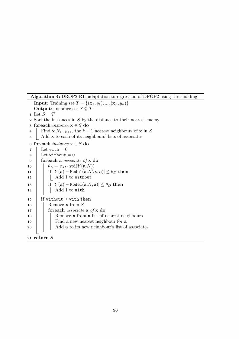
Algorithm 4: DROP2-RT: adaptation to regression of DROP2 using thresholding

Input: Training set T = {(x1, y1), ..., (xn, yn)}Output: Instance set S ⊆ T

1 Let S = T2 Sort the instances in S by the distance to their nearest enemy3 foreach instance x ∈ S do4 Find x.N1...k+1, the k + 1 nearest neighbours of x in S5 Add x to each of its neighbours’ lists of associates

6 foreach instance x ∈ S do7 Let with = 08 Let without = 09 foreach a associate of x do

10 θD = αD · std(Y (a.N))11 if |Y (a)− Model(a.N\x,a)| ≤ θD then12 Add 1 to without

13 if |Y (a)− Model(a.N,a)| ≤ θD then14 Add 1 to with

15 if without ≥ with then16 Remove x from S17 foreach associate a of x do18 Remove x from a list of nearest neighbours19 Find a new nearest neighbour for a20 Add a to its new neighbour’s list of associates

21 return S

96

neighbours and associates of each instance, iii) calculation of the values of variable with

and without, iv) using the values of these variables a decision is made of accepting orrejecting the instances as part of the selected subset.

The proposed methods use the neighbour and associate sets of each instance to cal-culate the values of variables with and without (or the variables eWith and eWithout

with a similar role in the algorithm), as the methods on which they are based, and hencethey have the same algorithmic complexity of the DROP family for classification.

The main difference is in how the variables with and without are calculated:

• Using Error accumulation: variables accumulate the error produced by the regressor(Model) on each of the instances, and therefore, they have real values.

• Using thresholding: variables are counters that increase their values depending onwhether the difference of the regressor prediction (Model) and the actual valueexceeds a threshold θD.

Besides the way these variables are calculated, the initial sorting and noise filteringof instances have had to be adapted to regression. Sorting was done as explained inSection 3.2.1, and for noise filtering, the algorithm RegENN (see Algorithm 3) has beenused.

4. Experiments and results

This section evaluates the performance of the four methods proposed in the precedingsection. They were compared between each other, against an instance selection algorithmfor regression called RegCNN [25] and against the baseline of training the regressorwithout filtering. Finally, the robustness to noise of the new algorithms was tested.

4.1. Experimental setup

Experiments were performed using several datasets, several instance selection meth-ods and several regressors. For each combination of these 3 elements, we applied a 10-foldcross validation [13]. The 10-fold cross validation was as following, each dataset was splitinto 10 subsets, the union of 9 of the subsets was reduced using instance selection andthe resultant subset was used to train a regressor. The accuracy was calculated usingthe 10-th subset that was not used in the training phase.

Instance selection can be thought of as a multi-objective problem: on the one hand,it attempts to reduce the size of the resulting dataset and, on the other, to minimize theerror [29]. Therefore, if we want a fair comparison of the results, considering accuracyonly would not be the best approach. We have used the same idea as in [28] to combineboth the retention rate and the error in a single index:

Iω = ω · ε+ (1− ω) ·m (1)

where ε is the error (calculated as 1−R2), ω is a value in the interval [0, 1] that assignsgreater importance to the accuracy or to the reduction of storage space, and m is theretention ratio, expressed as:

m =|S||T | (2)

97

where, |S| is the number of instances retained by the instance selection algorithm, and|T | is the number of instances in the original dataset. The smaller the value of Iω, themore favourable the results, as high values represent little reduction (higher retentionratio) and/or high error, however, lower values indicate greater reduction in the filtereddataset (lower retention ratio) and/or greater accuracy.

To measure the accuracy, we have chosen the correlation coefficient (R2) [10] sinceits value is in the interval [0, 1] and we can use it directly in the Equation 1.

4.2. Configurations

The experiments were performed in Weka [43], implementing the instance selectionmethods as Weka filters. The regressors used were:

• nearest neighbours (with k = 8).

• multilayer perceptron (trained with backpropagation with the following parameters:learning rate = 0.3, momentum = 0.2, number of hidden neurons = #attr+1

2 ).

• REPTrees (with Weka default parameters).

Nevertheless, the exact regressors are not of extreme relevance to the study, as whatwe want to compare is the improvement or deterioration of the predictive ability wheninstance selection is applied.

The parameters of the instance selection methods were the following. The kNNnearest neighbour regressor was used as Model, with k = 9 (the value suggested in [25]).In the threshold-based methods (DROP2-RT and DROP3-RT), the value of αD was 0.5(the value that gave the best results in previous analyses). The best values of αE werechosen after testing the values 1, 2, 3, 4 and 5. Table 1 shows the optimal values for thedifferent adaptations to regression of DROP, the various regressors, and different levelsof noise (see Section 4.5 for details of the analysis of robustness to noise).

Note that RegENN is a kind of noise filter so θE should be larger than the standarddeviation of the output value of the neighbours, as only the outliers should be rejected,which is why αE is bigger than 1, with αE < 1 the noise filtering would be too aggressive[25]. This is not the case for DROP algorithms and the value of αD. If αD > 1, θD wouldbe too large and it would be harder to detect the effect of removing an instance fromthe dataset (the conditions in lines 11 and 13 would almost always be false, the variableswith and without would not be adapted, and the instances would be systematicallyremoved from the dataset. In other words, the instance selection process would be tooaggressive at removing instances).

RegCNN is influenced by two parameters α and k. With the aim to use reasonablevalues for these parameters, we first launched several experiments with different values:0.25, 0.5, 0.75 and 1 for α; and 3, 5, 7 and 9 for k. The best results, for all regressors, wereachieved using α = 0.25. Whereas the optimal values for k depended on the regressorand the level of noise of the datasets, they are shown in Table 2.

4.3. Datasets

The datasets used for experimentation were obtained from the KEEL repository [2].They are described in Table 3, which details the number of attributes, the number of

98

Table 1: Value of αE which has achieved lower errors for the different regressors and noise levels (seeSection 4.5 on noise tolerance).

Noise IS algorithm kNN MLP REPTree

0 %DROP3-RE 5 5 3DROP2-RT 4 2 1DROP3-RT 4 5 2




Table 2: Value of k for RegCNN which has achieved lower errors for the different regressors and noiselevels (see Section 4.5 on noise tolerance).

Noise kNN MLP REPTree

0 % 9 9 910 % 3 7 320 % 9 7 930 % 7 7 7

99

Table 3: Datasets used in the experiments

Dataset # attributes # instancesCorrelation coefficient

kNN MLP REPTree

1 MachineCPU 6 209 0.9335 0.9433 0.81272 Baseball 16 337 0.8291 0.7350 0.77753 DEE 6 365 0.9013 0.9061 0.86314 AutoMPG8 7 392 0.9276 0.9330 0.91335 AutoMPG6 5 392 0.9345 0.9277 0.90816 Ele-1 2 495 0.8321 0.8402 0.79697 Stock 9 950 0.9927 0.9864 0.98328 Laser 4 993 0.9725 0.9873 0.95279 Concrete 8 1 030 0.8296 0.9103 0.8978

10 Treasury 15 1 049 0.9974 0.9981 0.995511 Mortgage 15 1 049 0.9981 0.9995 0.996512 Ele-2 4 1 056 0.9904 0.9969 0.995013 Friedman 5 1 200 0.9425 0.9135 0.849514 Wizmir 9 1 461 0.9930 0.9967 0.992615 Wankara 9 1 609 0.9924 0.9964 0.991216 Plastic 2 1 650 0.8773 0.9024 0.860617 Quake 3 2 178 0.1074 0.0808 0.069918 ANACALT 7 4 052 0.9755 0.9890 0.989819 Abalone 8 4 177 0.7253 0.7516 0.691820 Delta-ail 5 7 129 0.8267 0.8314 0.803521 Compactiv 21 8 192 0.9860 0.9903 0.983922 Puma32h 32 8 192 0.4286 0.3200 0.956223 Delta-elv 6 9 517 0.7768 0.7913 0.776024 Ailerons 40 13 750 0.8966 0.8947 0.872825 Pole 26 14 998 0.9807 0.9491 0.985126 Elevators 18 16 599 0.8487 0.9499 0.844827 California 8 20 640 0.8438 0.8468 0.861228 House 16 22 784 0.6863 0.6736 0.682729 Mv 10 40 768 0.9853 0.9999 0.9995

instances and the correlation coefficient (R2) [10] for the regressors used in the experi-ments: nearest neighbour (kNN), multilayer perceptron (MLP) and REPTree (ReducedError-Pruning Tree) [43]. The only transformation performed on the data was the nor-malization of all the input attributes so that they appear in the range [0, 1]. This trans-formation is intended to prevent certain attributes with a lot of variance from distortingthe results in the calculation of the nearest neighbour.

4.4. Results and discussion

In the experiments, besides the proposed methods, we have included the methodRegCNN, a state-of-the-art method explained earlier, and the regressor trained with theunfiltered dataset. The obtained results are compared using the Iω index for differentvalues of ω.

100

0.00 0.10 0.20 0.30 0.40 0.50 0.60 0.70 0.80 0.90 1.000%

10%

20%

30%

40%

50%

60%

70%

80%

90%

100%

RegCNN DROP2-RE DROP3-RE DROP2-RT DROP3-RT Original

ω value

(a) kNN

0.00 0.10 0.20 0.30 0.40 0.50 0.60 0.70 0.80 0.90 1.000%

10%

20%

30%

40%

50%

60%

70%

80%

90%

100%


ω value

(b) Multilayer Perceptron

0.00 0.10 0.20 0.30 0.40 0.50 0.60 0.70 0.80 0.90 1.000%

10%

20%

30%

40%

50%

60%

70%

80%

90%

100%


ω value

(c) REPTree

Figure 1: Comparison of the instance selection methods. In x axis the value of Iω (see Eq. 1) is shown forω values in the range [0, 1]. On the y axis, a percentage of datasets are represented in which a methodis better than all the other approaches according to the evaluation index Iω . The extreme left-hand-sideof figures, (ω = 0) corresponds to the results when only the reduction of the dataset is considered; theextreme right-hand-side, (ω = 1) corresponds to the results for which only accuracy is considered ofrelevance and, on the middle (ω = 0.5), the same relevance is given to accuracy and reduction. Themethod called ‘Original’ refers to the regressor trained with the original dataset.

0.00 0.10 0.20 0.30 0.40 0.50 0.60 0.70 0.80 0.90 1.001

2

3

4

5

6

RegCNN DROP2-RE DROP3-RE DROP2-RT DROP3-RT

Original

ω value

(a) kNN

0.00 0.10 0.20 0.30 0.40 0.50 0.60 0.70 0.80 0.90 1.001

2

3

4

5

6


Original

ω value


0.00 0.10 0.20 0.30 0.40 0.50 0.60 0.70 0.80 0.90 1.001

2

3

4

5

6


Original

ω value

(c) REPTree

Figure 2: Comparison of average ranks for the instance selection methods (and the regressor withoutinstance selection, shown as ‘Original’ in the legend) for all ω values in the range [0, 1] (axis x). Axis yplots the average rank (according to the evaluation index Iω), low values are best, high values are worse.

Figure 1 shows the percentage of datasets for which a method is better than the rest.For ω = 1, that is, considering accuracy alone, it is observed that the best value of theindex is for the regressor trained with the original dataset (irrespective of the regressor).From that value, as greater importance is assigned to the reduction, the instance selectionalgorithms compete between each other. Thus, for ω < 1, as the dataset reductionincreases its weight in the index, DROP3-RT and DROP2-RT dominate the results forkNN and MLP, and DROP3-RT dominates for REPTree.

Average ranks [12] were used for comparing all the methods and were calculated in thefollowing way: the results for each dataset were sorted according to their performance,assigning rank 1 to the best, rank 2 to the second best, and so on. In the case of a tie,the range is divided between all the tied methods. The average rank for each methodis the mean value of all the datasets. Figure 2 shows the average ranks on the y axisplotted against the different values of ω on the x axis.

DROP3-RE for kNN and DROP2-RE for MLP and REPTree are the more conser-

101

Table 4: Average retention ratio (m). m is calculated as |S|/|T |, where |S| is the number of instancesretained by the instance selection algorithm, and |T | is the number of instances in the original set.

IS algorithms Average m

DROP2-RT 0.471DROP3-RT 0.468DROP2-RE 0.634DROP3-RE 0.631RegCNN 0.787

vative algorithms. If only accuracy is taken into account, these methods are the onesthat comes closest to the result of the regressor trained on the original dataset. Ac-cording to the ranking, RegCNN is in the middle between the regressor trained on theoriginal dataset and the regressor trained with the selected subsets obtained with theproposed algorithms, again if compression is not taken into account. On the other hand,threshold-based approaches, DROP2-RT and DROP3-RT, yield good results for ω valueslower than 0.9 or 0.95. Of these two, DROP3-RT is clearly better when the regressor isMLP or REPTree.

On the extreme left-hand-side of figures, (ω = 0) corresponds to the results whenconsidering only the reduction of the dataset; on the extreme right-hand-side, (ω = 1)corresponds to the results for which only accuracy is considered of relevance. In eachof these cases, the test of significance through the Hochberg procedure [23] has beencalculated (Tables 5, 6, 7 and 8). The algorithm with best result (the one with lowestrank) is significantly better than the others when the value in column ‘p Hoch.’ is lessthan 0.1 (significance level: 0.9) or less than 0.05 (significance level: 0.95).

Since mean ranking only offers an order between the methods, Table 4 shows the aver-age retention ratio of the different instance selection methods tested in the experiments.Whereas threshold methods have around 0.47 retention ratio, ie 53% of compression,methods based on error accumulation have around 0.63. On the other hand, RegCNNachieves the highest retention ratio, around 15% more than the most conservative of ouralgorithms (DROPx-RE). As it was expected, DROP2-Rx algorithms are more conserva-tive than DROP3-Rx algorithms because DROP3-Rx algorithms have an initial filteringstage that reduces the dataset.

As explained in [24], instance selection techniques are computationally expensive.Both, CNN and DROP for classification, share a complexity of O(n3), and the adaptationof these methods to regression inherits this complexity. If the average rank of the methodsaccording to their filtering time is obtained for all datasets, RegCNN is the best andsignificant better than all DROPx-Rx. This can be explained by the fact that incrementalmethods are faster than decremental ones [42], also the calculations of DROP are moreelaborated than those made in CNN. We have also compared the four proposed methodsbetween each other. The fastest was DROP2-RE, this was expected since this methodhas not initial sorting, as DROP2-RT, nor initial noise filtering, as DROP3-Rx.

However, the aim of instance selection is to reduce the dataset that will be used totrain. The reduction of training dataset implies, in lazy learning algorithms like kNN,the decrease in testing time. Whereas the training phase is executed only once and can

102

be made batch, the speed in the testing phase is crucial because it is executed multipletimes and, in many applications, the execution time should be as low as possible. Ifthe methods are ranked according to their execution time in the testing phase for alldatasets, DROP3-RT ranks the first followed by DROP3-RE and the others. Moreoverthe differences between DROP3-RT and DROP2-Rx, RegCNN and kNN are significantat 95% of confidence.

4.5. Noise tolerance

Real datasets contain noise [15] and their presence reduces the predictive capabilityof the learning algorithms. The instance selection methods may also be sensitive to thepresence of noise and atypical values (outliers) [5]. In fact, in addition to the reductionof the training set, one of the great benefits that the selection methods present is theircapability to reduce noise, and the elimination of outliers. Hence, it was considered ofinterest to perform a study of the robustness of these methods in the face of noise.

In classification, the characterization of the different types of noise, and how to in-troduce them in experimental validation have been investigated in depth (ie [45, 46]).On the contrary, in regression, what is considered noise and how to properly introduceit in the experimental validation is not that clear. In the experiments that were carriedout, the noise was introduced by exchanging the output values of two randomly selectedinstances. This way, the distribution of the sample, both for the input variables and forthe output variables was not modified.

Experiments were performed with 10%, 20% and 30% noise. Figures 3 and 4 showthe robustness of the proposed methods. DROP3-RE performs an excellent task as anoise filter. For all the classifiers, the precision that is obtained was better when thefiltered set was used than when the totality of the dataset was used. This behaviour wasrepeated as the noise that was introduced increased: 20% in figures 5 and 6, and 30% infigures 7 and 8.

Besides, DROP2-RT, for levels of noise of 20% and 30%, showed poor behaviour whenonly accuracy was considered (ω = 1), because as may be observed, the classifiers trainedwith the original noisy set yielded better values than when they were trained with thereduced set that was obtained by DROP2-RT. Nevertheless, this behaviour may be dueto a more aggressive reduction of the dataset in DROP2-RT, because as may be seen fromthe figures, DROP2-RT is, together with DROP3-RT, the algorithm that shows the bestbehaviour, if we look only at the reduction of the datasets (ω = 0). It is interesting tohighlight that DROP3-RT for the values of ω ≤ 0.9 is the one which, in general, obtainedbetter results, both for the original datasets and for the noisy datasets (DROP2-RT onlyappears to be at its same level for the k-NN classifier and for a noise of 10%).

As previously explained, Table 5 shows the ranking and the results of the Hochbergprocedure for each of the methods taking into account only the reduction in size of the setof instances that were selected. Both in the original sets and in the tests completed withnoise, DROP3-RT was, at a confidence level of 95%, significantly better than the error-based methods (DROP2-RE and DROP3-RE) and RegCNN. No significant differenceswere observed between DROP3-RT and DROP2-RT.

Tables 6, 7 and 8 show the ranking calculated over the accuracy (ω = 1) of kNN,MLP and REPTree trained with the set returned by the instance selection algorithms.The result of training the regressor without previous filtering (Original) is included in

103

0.00 0.10 0.20 0.30 0.40 0.50 0.60 0.70 0.80 0.90 1.000%

10%

20%

30%

40%

50%

60%

70%

80%

90%

100%


ω value

(a) kNN

0.00 0.10 0.20 0.30 0.40 0.50 0.60 0.70 0.80 0.90 1.000%

10%

20%

30%

40%

50%

60%

70%

80%

90%

100%


ω value


0.00 0.10 0.20 0.30 0.40 0.50 0.60 0.70 0.80 0.90 1.000%

10%

20%

30%

40%

50%

60%

70%

80%

90%

100%


ω value

(c) REPTree

Figure 3: Experiments with a noise level of 10%, the proposed methods are compared against RegCNNfor all ω values in the range [0, 1] (axis x). The y axis shows the percentage of datasets for which amethod is better than the rest according to the evaluation index Iω .

0.00 0.10 0.20 0.30 0.40 0.50 0.60 0.70 0.80 0.90 1.001

2

3

4

5

6


Original

ω value

(a) kNN

0.00 0.10 0.20 0.30 0.40 0.50 0.60 0.70 0.80 0.90 1.001

2

3

4

5

6


Original

ω value


0.00 0.10 0.20 0.30 0.40 0.50 0.60 0.70 0.80 0.90 1.001

2

3

4

5

6


Original

ω value

(c) REPTree

Figure 4: Experiments with a noise level of 10%, the proposed methods are compared against RegCNNfor all ω values in the range [0, 1] (axis x). The y axis shows the average rank (according to the evaluationindex Iω), low values are better, high values are worse.

0.00 0.10 0.20 0.30 0.40 0.50 0.60 0.70 0.80 0.90 1.000%

10%

20%

30%

40%

50%

60%

70%

80%

90%

100%


ω value

(a) kNN

0.00 0.10 0.20 0.30 0.40 0.50 0.60 0.70 0.80 0.90 1.000%

10%

20%

30%

40%

50%

60%

70%

80%

90%

100%


ω value


0.00 0.10 0.20 0.30 0.40 0.50 0.60 0.70 0.80 0.90 1.000%

10%

20%

30%

40%

50%

60%

70%

80%

90%

100%


ω value

(c) REPTree

Figure 5: Experiments with a noise level of 20%, the proposed methods are compared against RegCNNfor all ω values in the range [0, 1] (axis x). The y axis show the percentage of datasets for which amethod is better than the rest according to the evaluation index Iω .

104

0.00 0.10 0.20 0.30 0.40 0.50 0.60 0.70 0.80 0.90 1.001

2

3

4

5

6


Original

ω value

(a) kNN

0.00 0.10 0.20 0.30 0.40 0.50 0.60 0.70 0.80 0.90 1.001

2

3

4

5

6


Original

ω value


0.00 0.10 0.20 0.30 0.40 0.50 0.60 0.70 0.80 0.90 1.001

2

3

4

5

6


Original

ω value

(c) REPTree

Figure 6: Experiments with a noise level of 20%, the proposed methods are compared against RegCNNfor all ω values in the range [0, 1] (axis x). The y axis shows the average rank (according to the evaluationindex Iω), low values are better, high values are worse.

0.00 0.10 0.20 0.30 0.40 0.50 0.60 0.70 0.80 0.90 1.000%

10%

20%

30%

40%

50%

60%

70%

80%

90%

100%


ω value

(a) kNN

0.00 0.10 0.20 0.30 0.40 0.50 0.60 0.70 0.80 0.90 1.000%

10%

20%

30%

40%

50%

60%

70%

80%

90%

100%


ω value


0.00 0.10 0.20 0.30 0.40 0.50 0.60 0.70 0.80 0.90 1.000%

10%

20%

30%

40%

50%

60%

70%

80%

90%

100%


ω value

(c) REPTree

Figure 7: Experiments with a noise level of 30%, the proposed methods are compared against RegCNNfor all ω values in the range [0, 1] (axis x). The y axis shows the percentage of datasets for which amethod is better than the rest according to the evaluation index Iω .

0.00 0.10 0.20 0.30 0.40 0.50 0.60 0.70 0.80 0.90 1.001

2

3

4

5

6


Original

ω value

(a) kNN

0.00 0.10 0.20 0.30 0.40 0.50 0.60 0.70 0.80 0.90 1.001

2

3

4

5

6


Original

ω value


0.00 0.10 0.20 0.30 0.40 0.50 0.60 0.70 0.80 0.90 1.001

2

3

4

5

6


Original

ω value

(c) REPTree

Figure 8: Experiments with a noise level of 30%, the proposed methods are compared against RegCNNfor all ω values in the range [0, 1] (axis x). The average rank (according to the evaluation index Iω) isshown on the y axis, low values are better, high values are worse.

105

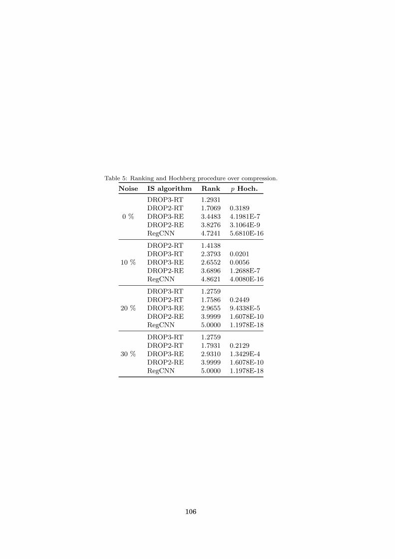
Table 5: Ranking and Hochberg procedure over compression.

Noise IS algorithm Rank p Hoch.

0 %

DROP3-RT 1.2931DROP2-RT 1.7069 0.3189DROP3-RE 3.4483 4.1981E-7DROP2-RE 3.8276 3.1064E-9RegCNN 4.7241 5.6810E-16

10 %

DROP2-RT 1.4138DROP3-RT 2.3793 0.0201DROP3-RE 2.6552 0.0056DROP2-RE 3.6896 1.2688E-7RegCNN 4.8621 4.0080E-16

20 %


30 %


106

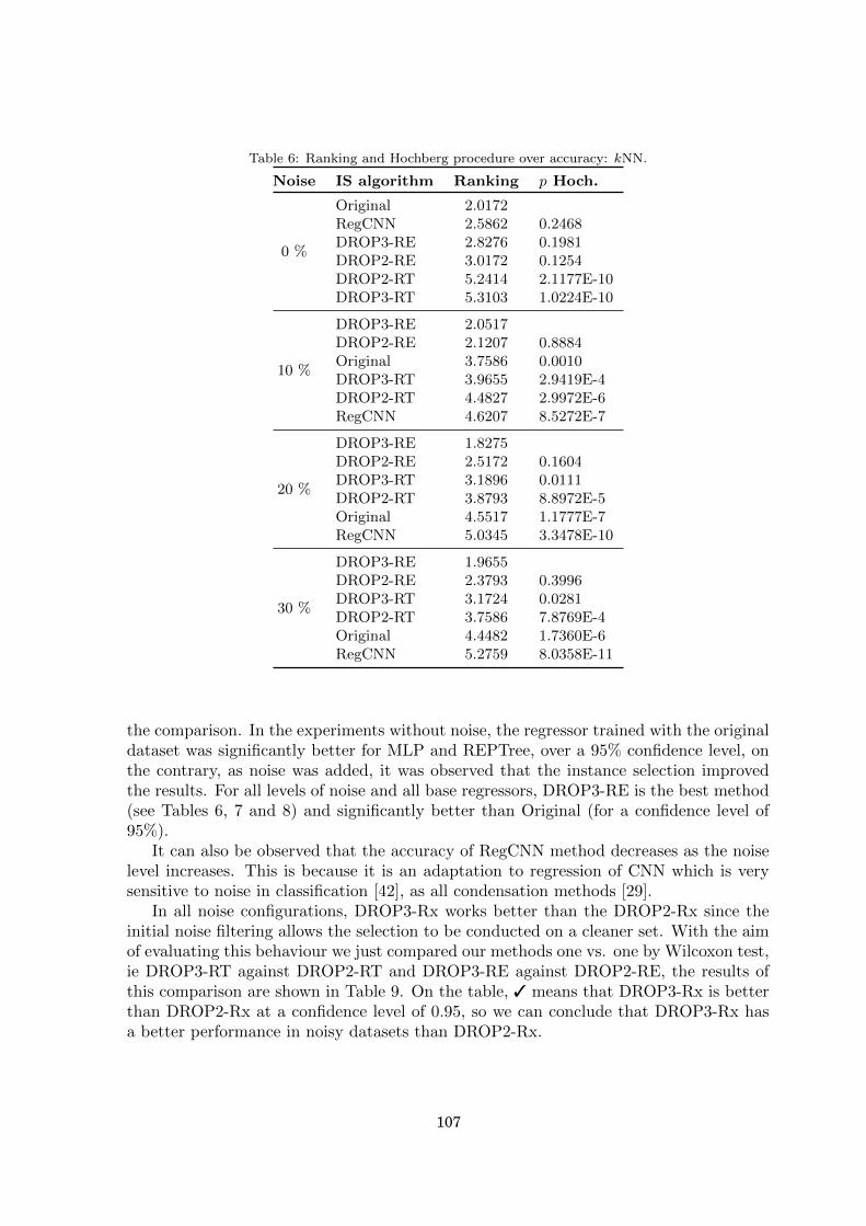
Table 6: Ranking and Hochberg procedure over accuracy: kNN.

Noise IS algorithm Ranking p Hoch.

0 %

Original 2.0172RegCNN 2.5862 0.2468DROP3-RE 2.8276 0.1981DROP2-RE 3.0172 0.1254DROP2-RT 5.2414 2.1177E-10DROP3-RT 5.3103 1.0224E-10

10 %

DROP3-RE 2.0517DROP2-RE 2.1207 0.8884Original 3.7586 0.0010DROP3-RT 3.9655 2.9419E-4DROP2-RT 4.4827 2.9972E-6RegCNN 4.6207 8.5272E-7

20 %

DROP3-RE 1.8275DROP2-RE 2.5172 0.1604DROP3-RT 3.1896 0.0111DROP2-RT 3.8793 8.8972E-5Original 4.5517 1.1777E-7RegCNN 5.0345 3.3478E-10

30 %

DROP3-RE 1.9655DROP2-RE 2.3793 0.3996DROP3-RT 3.1724 0.0281DROP2-RT 3.7586 7.8769E-4Original 4.4482 1.7360E-6RegCNN 5.2759 8.0358E-11

the comparison. In the experiments without noise, the regressor trained with the originaldataset was significantly better for MLP and REPTree, over a 95% confidence level, onthe contrary, as noise was added, it was observed that the instance selection improvedthe results. For all levels of noise and all base regressors, DROP3-RE is the best method(see Tables 6, 7 and 8) and significantly better than Original (for a confidence level of95%).

It can also be observed that the accuracy of RegCNN method decreases as the noiselevel increases. This is because it is an adaptation to regression of CNN which is verysensitive to noise in classification [42], as all condensation methods [29].

In all noise configurations, DROP3-Rx works better than the DROP2-Rx since theinitial noise filtering allows the selection to be conducted on a cleaner set. With the aimof evaluating this behaviour we just compared our methods one vs. one by Wilcoxon test,ie DROP3-RT against DROP2-RT and DROP3-RE against DROP2-RE, the results ofthis comparison are shown in Table 9. On the table, 3 means that DROP3-Rx is betterthan DROP2-Rx at a confidence level of 0.95, so we can conclude that DROP3-Rx hasa better performance in noisy datasets than DROP2-Rx.

107

Table 7: Ranking and Hochberg procedure over accuracy: Multilayer Perceptron.


0 %

Original 2.1724RegCNN 2.8793 0.793DROP3-RE 3.4999 0.0051DROP2-RE 3.5172 0.0051DROP3-RT 4.5517 1.1990E-6DROP2-RT 4.5349 1.1990E-6

10 %

DROP3-RE 2.4310DROP2-RE 3.1035 0.1711DROP3-RT 3.3449 0.1258Original 3.7241 0.0255DROP2-RT 4.1896 0.0014RegCNN 4.2069 0.0014

20 %

DROP3-RE 2.2759DROP2-RE 2.9483 0.2328DROP3-RT 3.6034 0.0230Original 3.8621 0.0068DROP2-RT 3.9655 0.0043RegCNN 4.2586 5.6637E-4

30 %

DROP3-RE 2.3276DROP3-RT 2.6724 0.4828DROP2-RE 2.9655 0.3883DROP2-RT 4.2069 3.9208E-4Original 4.2069 9.9208E-4RegCNN 4.6207 1.5253E-5

108

Table 8: Ranking and Hochberg procedure over accuracy: REPTree.


0 %

Original 1.3793RegCNN 2.7759 0.0045DROP2-RE 3.3103 1.6959E-4DROP3-RE 3.7414 4.5790E-6DROP3-RT 4.6207 1.6725E-10DROP2-RT 5.1724 5.7943E-14

10 %

DROP3-RE 2.0862DROP2-RE 2.9655 0.0735Original 3.3793 0.0170DROP3-RT 3.8103 0.0013RegCNN 4.2414 4.6046E-5DROP2-RT 4.5172 3.7465E-6

20 %

DROP3-RE 1.9138DROP2-RE 2.9310 0.0384Original 3.3793 0.0057DROP3-RT 3.7069 7.8769E-4RegCNN 4.1724 1.7128E-5DROP2-RT 4.8965 6.3515E-9

30 %

DROP3-RE 2.1379DROP3-RT 3.1724 0.0352DROP2-RE 3.3103 0.0340Original 3.7069 0.0042DROP2-RT 4.1207 2.1775E-4RegCNN 4.5517 4.4838E-6

Table 9: Wilcoxon test over accuracy (ω = 1) in noisy datasets. 3 indicates that DROP3-Rx is betterthan DROP2-Rx at a confidence level of 95% and “-” means no significant difference.

Noise DROP3-RT vs DROP2-RT DROP3-RE vs DROP2-RE

10 % 3 3

20 % 3 3

30 % 3 3

109

4.6. Benefits of using the proposed methods

Some remarkable observations can be made from the results, in this section we dis-cuss the main advantages and disadvantages of instance selection methods for regression.First, in contrast to instance selection for classification, the application of instance selec-tion methods in regression are not able to improve the accuracy of the original dataset,neither the proposed methods nor RegCNN. Second, the different approaches proposedto cope with regression have different characteristics: error accumulation (DROPx-RE)achieves lower reduction and consequently more accuracy whilst thresholding (DROPx-RT) achieves better reduction rate and lower accuracy. RegCNN achieves a good accu-racy at expense of the lowest retention rate. In addition, when RegCNN was applied overnoisy datasets, the instance selection method was strongly penalised. Nevertheless, themethods proposed based on DROP dealt with noise in a better way, outperforming theaccuracy achieved by the regressor trained over the whole noisy dataset. The robustnessin noisy environments is due to the filtering noise stage of DROP3-Rx, as DROP3 forclassification does.

5. Conclusions

In the paper, two new approaches have been introduced to adapt the family of DROPinstance selection methods, so successfully used for classification, to regression. Usingthese approaches four new algorithms for instance selection for regression have been pro-posed. It is an interesting contribution given that currently there are no many instanceselection methods for regression. The proposed methods have been subjected to bench-mark testing, where they were compared against each other, against RegCNN, one of thefew methods for this kind of Machine Learning task, and against the result obtained froma regressor trained with the original dataset. The regressors used were: a method basedon instances (kNN), a multilayer perceptron, and a method for constructing regressiontrees (REPTree).

We have discussed two approaches to adapt the DROP algorithms: using the errorfor the calculation of the variables with and without, and using the concept of soft classdefined by means of an adaptive threshold. The results are of interest as, although, inall methods, to a greater or lesser extent the predictive power is reduced, this reductionis low in comparison with the reduction of dataset size.

In addition, a comparison has been drawn with a dual approach of reduction andaccuracy to see how both objectives are related, as greater importance is given to onerather than another. In this way, the best algorithms is DROP3-RE in most casesif accuracy is to be maximised, as these methods are designed to minimize the lossof predictive capability of the resulting dataset. On the one hand, if the aim is tominimize the size of the datasets after selection, the best method is DROP3-RT both inthe experimentation with the original and with the noisy datasets.

A remarkable property of the proposed adaptations of DROP for regression is theirrobustness in the presence of noise. The experiments carried out with noise levels of10%, 20% and 30% have shown that the proposed instance selection algorithms are notonly able to reduce the size of the training dataset, but they are also able to reduce thenoise and significantly improve the accuracy achieved by different regressors.

110

6. Future lines

New instance selection methods for classification are still emerging, the use of thresh-olding makes it possible to adapt them directly to regression task. In future works weintend to adapt other promising instance selection methods with this idea, as for exam-ple [29].

In addition, the ideas presented in the paper can be applied to other fields like, forexample, feature selection. Feature selection is related with instance selection [16] but,unlike instance selection, algorithms try to find the best subset of features, not instances.The similarities between both techniques suggest that these ideas could be achieve goodresults too.

Acknowledgments

This work was partially supported by the Spanish Ministry of Economy and Com-petitiveness through project TIN2011-24046.

References

[1] Rafael Alcala, Jesus Alcala-Fdez, Francisco Herrera, and Jose Otero. Genetic learning of accurateand compact fuzzy rule based systems based on the 2-tuples linguistic representation. Interna-tional Journal of Approximate Reasoning, 44(1):45 – 64, 2007. Genetic Fuzzy Systems and theInterpretability–Accuracy Trade-off.

[2] Jesus Alcala-Fdez, Alberto Fernandez, Julian Luengo, Joaquın Derrac, and Salvador Garcıa. Keeldata-mining software tool: Data set repository, integration of algorithms and experimental analysisframework. Multiple-Valued Logic and Soft Computing, 17(2-3):255–287, 2011.

[3] M. Antonelli, P. Ducange, and F. Marcelloni. Genetic training instance selection in multiobjectiveevolutionary fuzzy systems: A coevolutionary approach. Fuzzy Systems, IEEE Transactions on,20(2):276–290, April 2012.

[4] Ricardo Barandela, Francesc J. Ferri, and Jose Salvador Sanchez. Decision boundary preservingprototype selection for nearest neighbor classification. IJPRAI, 19(6):787–806, 2005.

[5] Eric Bauer and Ron Kohavi. An empirical comparison of voting classification algorithms: Bagging,boosting, and variants. Machine Learning, 36(1-2):105–139, 1999.

[6] Marcin Blachnik and Miros law Kordos. Bagging of instance selection algorithms. In LeszekRutkowski, Marcin Korytkowski, Rafa l Scherer, Ryszard Tadeusiewicz, LotfiA. Zadeh, and JacekM.Zurada, editors, Artificial Intelligence and Soft Computing, volume 8468 of Lecture Notes in Com-puter Science, pages 40–51. Springer International Publishing, 2014.

[7] Henry Brighton and Chris Mellish. On the consistency of information filters for lazy learning

algorithms. In JanM. Zytkow and Jan Rauch, editors, Principles of Data Mining and KnowledgeDiscovery, volume 1704 of Lecture Notes in Computer Science, pages 283–288. Springer BerlinHeidelberg, 1999.

[8] Henry Brighton and Chris Mellish. Advances in instance selection for instance-based learningalgorithms. Data Mining and Knowledge Discovery, 6:153–172, 2002.

[9] Jorge Calvo-Zaragoza, Jose J. Valero-Mas, and Juan R. Rico-Juan. Improving kNN multi-labelclassification in prototype selection scenarios using class proposals. Pattern Recognition, 48(5):1608– 1622, 2015.

[10] A. Colin Cameron and Frank A.G. Windmeijer. An R-squared measure of goodness of fit for somecommon nonlinear regression models. Journal of Econometrics, 77(2):329 – 342, 1997.

[11] Nitesh V. Chawla, Lawrence O. Hall, Kevin W. Bowyer, and W. Philip Kegelmeyer. Learningensembles from bites: A scalable and accurate approach. J. Mach. Learn. Res., 5:421–451, December2004.

[12] Janez Demsar. Statistical comparisons of classifiers over multiple data sets. J. Mach. Learn. Res.,7:1–30, December 2006.

111

[13] T.G. Dietterich. Approximate statistical tests for comparing supervised classification learning al-gorithms. Neural computation, 10(7):1895–1923, 1998.

[14] S. Garcia, J. Derrac, J.R. Cano, and F. Herrera. Prototype selection for nearest neighbor classifi-cation: Taxonomy and empirical study. Pattern Analysis and Machine Intelligence, IEEE Trans-actions on, 34(3):417–435, March 2012.

[15] Cesar Garcıa-Osorio, Aida de Haro-Garcıa, and Nicolas Garcıa-Pedrajas. Democratic instanceselection: A linear complexity instance selection algorithm based on classifier ensemble concepts.Artificial Intelligence, 174(5-6):410 – 441, 2010.

[16] Nicolas Garcıa-Pedrajas, Aida de Haro-Garcıa, and Javier Perez-Rodrıguez. A scalable approachto simultaneous evolutionary instance and feature selection. Information Sciences, 228:150 – 174,2013.

[17] G W Gates. The reduced nearest neighbor rule. IEEE Transactions on Information Theory,IT-18:431–433, May 1972.

[18] David E. Goldberg. Genetic Algorithms in Search, Optimization and Machine Learning. Addison-Wesley Longman Publishing Co., Inc., Boston, MA, USA, 1st edition, 1989.

[19] Marek Grochowski and Norbert Jankowski. Artificial Intelligence and Soft Computing - ICAISC2004: 7th International Conference, Zakopane, Poland, June 7-11, 2004. Proceedings, chapterComparison of Instance Selection Algorithms II. Results and Comments, pages 580–585. SpringerBerlin Heidelberg, Berlin, Heidelberg, 2004.

[20] A. Guillen, L.J. Herrera, G. Rubio, H. Pomares, A. Lendasse, and I. Rojas. New method forinstance or prototype selection using mutual information in time series prediction. Neurocomputing,73(10–12):2030 – 2038, 2010. Subspace Learning / Selected papers from the European Symposiumon Time Series Prediction.

[21] P. Hart. The condensed nearest neighbor rule (corresp.). Information Theory, IEEE Transactionson, 14(3):515 – 516, may 1968.

[22] Francisco Herrera. Genetic fuzzy systems: taxonomy, current research trends and prospects. Evo-lutionary Intelligence, 1(1):27–46, 2008.

[23] Yosef Hochberg. A sharper bonferroni procedure for multiple tests of significance. Biometrika,75(4):800–802, 1988.

[24] Norbert Jankowski and Marek Grochowski. Artificial Intelligence and Soft Computing - ICAISC2004: 7th International Conference, Zakopane, Poland, June 7-11, 2004. Proceedings, chapterComparison of Instances Seletion Algorithms I. Algorithms Survey, pages 598–603. Springer BerlinHeidelberg, Berlin, Heidelberg, 2004.

[25] Miros law Kordos and Marcin Blachnik. Instance selection with neural networks for regressionproblems. In Artificial Neural Networks and Machine Learning - ICANN 2012, volume 7553 ofLecture Notes in Computer Science, pages 263–270. Springer Berlin Heidelberg, 2012.

[26] S.B. Kotsiantis, I.D. Zaharakis, and P.E. Pintelas. Machine learning: a review of classification andcombining techniques. Artificial Intelligence Review, 26(3):159–190, 2006.

[27] Nojun Kwak and Jung-Won Lee. Feature extraction based on subspace methods for regressionproblems. Neurocomputing, 73(10-12):1740 – 1751, 2010. Subspace Learning / Selected papersfrom the European Symposium on Time Series Prediction.

[28] E. Leyva, A. Gonzalez, and R. Perez. A set of complexity measures designed for applying meta-learning to instance selection. Knowledge and Data Engineering, IEEE Transactions on, 27(2):354–367, Feb 2015.

[29] Enrique Leyva, Antonio Gonzalez, and Raul Perez. Three new instance selection methods based onlocal sets: A comparative study with several approaches from a bi-objective perspective. PatternRecognition, 48(4):1523 – 1537, 2015.

[30] E. Marchiori. Class conditional nearest neighbor for large margin instance selection. PatternAnalysis and Machine Intelligence, IEEE Transactions on, 32(2):364–370, Feb 2010.

[31] Elena Marchiori. Hit miss networks with applications to instance selection. J. Mach. Learn. Res.,9:997–1017, June 2008.

[32] J. A. Olvera-Lopez, J. Fco. Martınez-Trinidad, J. A. Carrasco-Ochoa, and J. Kittler. Prototypeselection based on sequential search. Intell. Data Anal., 13(4):599–631, December 2009.

[33] J.Arturo Olvera-Lopez, J.Ariel Carrasco-Ochoa, J.Francisco Martınez-Trinidad, and Josef Kittler.A review of instance selection methods. Artificial Intelligence Review, 34(2):133–143, 2010.

[34] Jose A. Olvera-Lopez, J.Ariel Carrasco-Ochoa, and Jose Fco. Martınez-Trinidad. Sequential searchfor decremental edition. In Marcus Gallagher, James P. Hogan, and Frederic Maire, editors, Intel-ligent Data Engineering and Automated Learning - IDEAL 2005, volume 3578 of Lecture Notes inComputer Science, pages 280–285. Springer Berlin Heidelberg, 2005.

112

[35] JA Perez-Benıtez, JL Perez-Benıtez, and JH Espina-Hernandez. Novel data condensing methodusing a prototype’s front propagation algorithm. Engineering Applications of Artificial Intelligence,39(0):181 – 197, 2015.

[36] I. Rodriguez-Fdez, M. Mucientes, and A. Bugarin. An instance selection algorithm for regressionand its application in variance reduction. In Fuzzy Systems (FUZZ), 2013 IEEE InternationalConference on, pages 1–8, July 2013.

[37] Milos B. Stojanovic, Milos M. Bozic, Milena M. Stankovic, and Zoran P. Stajic. A methodology fortraining set instance selection using mutual information in time series prediction. Neurocomputing,141(0):236 – 245, 2014.

[38] J. Tolvi. Genetic algorithms for outlier detection and variable selection in linear regression models.Soft Computing, 8(8):527–533, 2004.

[39] Chih-Fong Tsai and Che-Wei Chang. SVOIS: Support vector oriented instance selection for textclassification. Information Systems, 38(8):1070 – 1083, 2013.

[40] D. Randall Wilson and Tony R. Martinez. Instance pruning techniques. In Machine Learning:Proceedings of the Fourteenth International Conference (ICML’97), pages 404–411. Morgan Kauf-mann, 1997.

[41] Dennis L. Wilson. Asymptotic properties of nearest neighbor rules using edited data. Systems,Man and Cybernetics, IEEE Transactions on, SMC-2(3):408–421, July 1972.

[42] D.Randall Wilson and Tony R. Martinez. Reduction techniques for instance-based learning algo-rithms. Machine Learning, 38(3):257–286, 2000.

[43] Ian H. Witten, Eibe Frank, and Mark A. Hall. Data Mining: Practical Machine Learning Toolsand Techniques. Morgan Kaufmann Publishers Inc., San Francisco, CA, USA, 3rd edition, 2011.

[44] Jianping Zhang, Yee-Sat Yim, and Junming Yang. Intelligent selection of instances for predictionfunctions in lazy learning algorithms. In DavidW. Aha, editor, Lazy Learning, pages 175–191.Springer Netherlands, 1997.

[45] Xingquan Zhu and Xindong Wu. Class noise vs. attribute noise: A quantitative study. ArtificialIntelligence Review, 22(3):177–210, 2004.

[46] Xingquan Zhu, Xindong Wu, and Qijun Chen. Eliminating class noise in large datasets. In InProceeding of International Conference on Machine Learning (ICML 2003), pages 920–927, 2003.

113

Big data marks the beginning of a majortransformation.

Mayer-Schönberger and Cukier (2013)

CH

AP

TE

R

4INSTANCE SELECTION OF LINEAR COMPLEXITY FOR BIG DATA

This journal paper presents a new instance selection method for classification with a

remarkable characteristic: linear complexity in the number of instances. In the paper,

two different algorithms are described: one is able to process instances in the on-fly mode

(i.e. with no need for the whole data set to fit in the memory) and the other performs the task in

two passes.

It is the concept of Local Sensitive Hashing (LSH) that makes linear complexity possible.

These families of hashing functions have a particular feature, instead of avoiding collisions they

attempt to place similar objects in the same bucket and different instances in other buckets.

Authors: Álvar Arnaiz-González, Jose-Francisco Díez-Pastor, Juan José Rodríguez-Diez, César García-

Osorio

Type: Journal

Published in: Knowledge-Based Systems 107: 83-95

Year: 2016

Reference: Arnaiz-González et al. (2016c)

115

Instance selection of linear complexity for big data

Álvar Arnaiz-González, José F. Díez-Pastor, Juan J. Rodríguez, César García-Osorio


Abstract

Over recent decades, database sizes have grown considerably. Larger sizes presentnew challenges, because machine learning algorithms are not prepared to process suchlarge volumes of information. Instance selection methods can alleviate this problem whenthe size of the data set is medium to large. However, even these methods face similarproblems with very large-to-massive data sets.

In this paper, two new algorithms with linear complexity for instance selection pur-poses are presented. Both algorithms use locality-sensitive hashing to �nd similaritiesbetween instances. While the complexity of conventional methods (usually quadratic,O(n2), or log-linear, O(n log n)) means that they are unable to process large-sized datasets, the new proposal shows competitive results in terms of accuracy. Even more re-markably, it shortens execution time, as the proposal manages to reduce complexity andmake it linear with respect to the data set size. The new proposal has been comparedwith some of the best known instance selection methods for testing and has also beenevaluated on large data sets (up to a million instances).

Keywords: nearest neighbor, data reduction, instance selection, hashing, big data

1. Introduction

The k nearest neighbor classi�er (kNN) [11], despite its age, is still widely used inmachine learning problems [9, 17, 20]. Its simplicity, straightforward implementationand good performance in many domains means that it is still in use, despite of some ofits �aws [37]. The kNN algorithm is included in the family of instance based learning,in particular within the lazy learners, as it does not build a classi�cation model but juststores all the training set [8]. Its classi�cation rule is simple: for each new instance,assign the class according to the majority vote of its k nearest neighbors in the trainingset, if k = 1, the algorithm only takes the nearest neighbor into account [45]. Thisfeature means that it requires a lot of memory and processing time in the classi�cationphase [48]. Traditionally, two paths have been followed to speed up the process: eitheraccelerate the calculation of the closest neighbors [3, 4], or decrease training set size bystrategically selecting only a small portion of instances or features [38].

Email addresses: [email protected] (Álvar Arnaiz-González), [email protected](José F. Díez-Pastor), [email protected] (Juan J. Rodríguez), [email protected](César García-Osorio)

Preprint submitted to Knowledge-Based Systems November 10, 2017

116

Regarding the acceleration of algorithms, perhaps one of the most representativeapproaches is to approximate nearest neighbors, a broadly researched technique in whichthe nearest neighbor search is done over a sub-sample of the whole data set [56]. In this�eld, many algorithms have been proposed for approximate nearest neighbor problems [3,4, 30, 34, 39].

The focus of this paper is on the second path, the reduction of data set size. Thereason is that this reduction is bene�cial for most methods rather than only those basedon nearest neighbors. Although we will only consider the reduction of instances (instanceselection) in this paper, the reduction could also be applied to attributes (feature selec-tion), or even both at the same time [51]. The problem is that the fastest conventionalinstance selection algorithms have a computational complexity of at least O(n log n) andothers are of even greater complexity.

The need for rapid methods for instance selection is even more relevant nowadays,given the growing sizes of data sets in all �elds of machine learning applications (suchas medicine, marketing or �nance [43]), and the fact that the most commonly used datamining algorithms for any data mining task were developed when the common databasescontained at most a few thousands of records. Currently, millions of records are themost common scenario. So, most data mining algorithms �nd many serious di�culties intheir application. Thus, a new term has emerged, �Big Data�, in reference to those datasets that, by volume, variability and speed, make the application of classical algorithmsdi�cult [44]. With regard to instance selection, the solutions that have appeared so farto deal with big data problems adopt the `divide and conquer' approach [13, 22]. Thealgorithms proposed in the present paper o�er a di�erent approach, just a sequential butvery quick and simple processing of each instance in the data set.

In particular, the major contribution of this paper is the use of Locality-SensitiveHashing (LSH) to design two new algorithms, which o�ers two main advantages:

• Linear complexity: the use of LSH means a dramatic reduction in the executiontime of the instance selection process. Moreover, these methods are able to dealwith huge data sets due to their linear complexity.

• On-the-�y processing: one of the new methods is able to tackle the instances inone step. It is not necessary for all instances �t in memory: a characteristic thato�ers a remarkable advantage in relation to big data.

The paper is organized as follows: Section 2 presents the reduction techniques back-ground, with special emphasis on the instance selection methods used in the experimentalvalidation; Section 3 introduces the concept of locality-sensitive hashing, the basis of theproposed methods which are presented in Section 4; Section 5 presents and analyzes theresults of the experiments and, �nally, sections 6 and 7 set out the conclusions andfuture research, respectively.

2. Reduction techniques

Available data sets are progressively becoming larger in size. As a consequence, manysystems have di�culties processing such data sets to obtain exploitable knowledge [23].The high execution times and storage requirements of the current classi�cation algorithmsmake them unusable when dealing with these huge data sets [28]. These problems can

117

be decisive, if a lazy learning algorithm such as the nearest neighbor rule is used, andcan even prevent results from being obtained. However, reducing the size of the dataset by selecting a representative subset has two main advantages: it reduces the memoryrequired to store the data and it accelerates the classi�cation algorithms [19].

In the scienti�c literature, the term �reduction techniques� includes [61]: prototypegeneration [32]; prototype selection [52] (when the classi�er is based on kNN); and (forother classi�ers) instance selection [8]. While prototype generation replaces the originalinstances with new arti�cial ones, instance selection and prototype selection attempt to�nd a representative subset of the initial training set that does not lessen the predic-tive power of the algorithms trained with such a subset [45]. In the paper, prototypegeneration is not addressed, however a complete review on it can be found in [57].

2.1. Instance selection

The aforementioned term �instance selection� brings together di�erent proceduresand algorithms that target the selection of a representative subset of the initial train-ing set. There are numerous instance selection methods for classi�cation, a completereview of which may be found in [21]. Instance selection has also been applied to bothregression [2, 33] and time series prediction [26, 55].

According to the order in which instances are processed, instance selection methodscan be classi�ed into �ve categories [21]. If they begin with an empty set and they addinstances to the selected subset, by means of analyzing the instances in the training set,they are called incremental. The decremental methods, on the contrary, start with theoriginal training data set and they remove those instances that are considered super�uousor unnecessary. Batch methods are those in which no instance is removed until all ofthem have been analyzed, instances are simply marked from removal if the algorithmdetermines that they are not needed, and at the end of the process only the unmarkedinstances are kept. Mixed algorithms start with a preselected set of instances. Theprocess then decides either to add or to delete the instances. Finally, �xed methods area sub-family of mixed ones, in which the number of additions and removals are the same.This approach allows them to maintain a �xed number of instances (more frequent inprototype generation).

Considering the type of selection, three categories may be distinguished. This crite-rion is mainly correlated with the points that they remove: either border points, centralpoints, or otherwise. Condensation techniques try to retain border points. Their underly-ing idea is that internal points do not a�ect classi�cation, because the boundaries betweenclasses are the keystone of the classi�cation process. Edition methods may be consideredthe opposite of condensation techniques, as their aim is to remove those instances thatare not well-classi�ed by their nearest neighbors. The edition process achieves smootherboundaries as well as noise removal. In the middle of those approaches are hybrid algo-rithms, which try to maintain or even to increase the accuracy capability of the data set,by removing both: internal and border points [21].

Evolutionary approaches for instance selection have shown remarkable results in bothreduction and accuracy. A complete survey of them can be found in [16]. However, themain limitation of those methods is their computational complexity [36]. This drawbackis the reason why they are not taken into account in this study, because the methods itproposes are oriented towards large data sets.

118

Table 1: Summary of state-of-the-art instance selection methods used in the experimental setup (taxon-omy from [21]; computational complexity from [31] and authors' papers).

Strategy Direction Algorithm Complexity Year Reference

Condensation Incremental CNN O(n3) 1968 [27]Incremental PSC O(n logn) 2010 [46]Decremental RNN O(n3) 1972 [25]Decremental MSS O(n2) 2002 [6]

Hybrid Decremental DROP1-5 O(n3) 2000 [60]Batch ICF O(n2) 2002 [8]Batch HMN-EI O(n2) 2008 [41]Batch LSBo O(n2) 2015 [37]

In the remaining part of this section, we give further details of the most representativemethods used in the experimental setup. A summary of the methods considered in thestudy can be seen in Table 1.

2.1.1. Condensation

The algorithm of Hart, Condensed Nearest Neighbor (CNN) [27] is considered the�rst formal proposal of instance selection for the nearest neighbor rule. The concept oftraining set consistency is important in this algorithm and is de�ned as follows: givena non empty set X (X 6= ∅), a subset S of X (S ⊆ X) is consistent with respect toX if, using the subset S as training set, the nearest neighbor rule can correctly classifyall instances in X. Following this de�nition of consistency, if we consider the set X asthe training set, a condensed subset should have the properties of being consistent and,ideally, smaller than X. After CNN appeared, other condensation methods emerged withthe aim of decreasing the size of the condensed data set, e.g.: Reduced Nearest Neighbor(RNN) [25]. One of the latest is the Prototype Selection by Clustering (PSC) [46], whichuses clustering to speed up the selection process. So, the use of clustering gives a highe�ciency to PSC, if compared against state-of-the-art methods, and better accuracy thanother clustering-based methods such as CLU [40].

In [6], the authors proposed a modi�cation to the de�nition of a selective subset [54],for a better approximation to decision borders. The selective subset can be thought of assimilar to the idea of the condensed algorithm of Hart, but applying a condition strongerthan the condition of consistency. The aim is to �nd the selected instances in an easierway, which is less sensitive to the random initialization of S and the order of explorationof X in Harts' algorithm. The subset obtained in this way is called the selective subset(SS ).

A subset S of the training set X is a selective subset (SS ), if it satis�es the followingconditions:

1. S is consistent (as in Harts' algorithm).2. All instances in the original training set, X, are closer to a selective neighbor (a

member of S) of the same class than to any instance of a di�erent class in X.

Then, the authors present a greedy algorithm which attempts to �nd selective in-stances starting with those instances of the training set that are close to the decision

119

boundary of the nearest neighbor classi�er. The algorithm presented is an e�cient al-ternative to the Selective algorithm [54] and it is usually able to select better instances(the ones closer to the boundaries).

2.1.2. Hybrid

One problem that arises when condensation methods are used is their noise sensitivity,while hybrid methods have speci�c mechanisms to make them more robust to noise [37].

The DROP (Decremental Reduction Optimization Procedure) [60] family of algo-rithms comprises some of the best instance selection methods for classi�cation [8, 47, 50].The instance removal criteria is based on two relations: associates and nearest neigh-bors. The relation of associate is the inverse of nearest neighbors: those instances p thathave q as one of their nearest neighbors are called associates of q. The set of nearestneighbors of one instance is called the neighborhood of the instance. For all instances,its list of associates is a list with all instances that have that particular instance in theirneighborhood.

Marchiori proposed a new graph-based representation of the data set called Hit MissNetworks (HMN) [41]. The graph has a directed edge from each instance to its near-est neighbor on the di�erent classes, with one edge per class. The information in thegraph was used to de�ne three new hybrid algorithms: HMN-E, HMN-C and HMN-EI.A couple of years later, HMNs were used to de�ne a new information-theoretic instancescoring method to de�ne a new instance selection method called Class Conditional Near-est Neighbor (CCIS) [42]. According to [21], HMN-EI is able to achieve more accuratedata sets than CCIS which is the reason why HMN-EI was used in experimental setup.

The local-set (LS) concept, proposed for the very �rst time in [7], is a powerful toolfor some machine learning tasks, including instance selection. A local-set of an instancex contains all those instances which are closer to x than its nearest neighbor of di�erentclass, its nearest enemy. The selection rule of the Iterative Case Filtering algorithm(ICF) [7] uses local sets to build two sets: coverage and reachability. These two conceptsare closely related to the neighborhood and associate list used in DROP algorithms. Thecoverage of an instance is its LS, that can be seen as a neighborhood of the instance that,instead of considering a �xed number k of neighbor, includes all instances closer to theinstance than its closest enemy. The reachable set of an instance is its set of associates.The coverage set of an instance is its neighborhood. The deletion rule is as follows: aninstance is removed from the data set if its reachable set (its set of associates) is biggerthan its coverage (its `neighborhood'). This rule means that the algorithm removes aninstance if other object exists that generalizes its information. To address the problem ofnoisy data sets, both ICF and DROP3, begin with a noise-�lter stage. Recently, Leyvaet al [37] presented three new instance selection methods based on LSs. Their hybridapproach, which o�ers a good balance between reduction and accuracy, is called Local SetBorder Selector (LSBo) and it uses a heuristic criterion: the instances in the boundariesbetween classes tend to have greater LSs. As is usual in hybrid methods, LSBo startswith a noise �ltering algorithm which was presented in the same paper called LSSm.

2.2. Scaling up instance selection

The main drawback of instance selection methods is their complexity that is quadraticO(n2), where n is the number of instances [22] or, at best, log-linear O(n log n); thus, the

120

majority of them are not applicable in data sets with hundreds or even many thousandsof instances [15]. Table 1 summarizes the computational complexity of the instanceselection methods used in the experimental section.

One approach to deal with massive data sets, is to divide the original problem intosmaller subsets of instances; known as strati�cation. The underlying idea of these meth-ods is to split the original data set into disjointed subsets, then an instance selectionalgorithm is applied to each subset [10, 13, 22, 24]. This approach is used in [22] where amethod was proposed that addressed the splitting process, using Grand Tour [5] theory,to achieve linear complexity.

The problem known as big data refers to the challenges and di�culties that arise whenhuge amounts of data are processed. One way to accelerate instance selection methodsand to be able to cope with massive data sets is adapt them to parallel environments [49].To do so, the way that algorithms work has to be redesigned. The MapReduce paradigmo�ers a robust framework with which to process huge data sets over clusters of machines.Following up on this idea, a new proposal was presented recently by Triguero et al. [58].

3. Locality-sensitive hashing

The locality-sensitive hashing (LSH ) is an e�cient method for checking similaritybetween elements. It makes a particular use of hash functions that, unlike those used inother applications of hashing1, seeks to allocate similar items to the same bucket witha high probability, and at the same time to greatly reduce the probability of assigningdissimilar items to the same bucket [35].

LSH use is common to increase the e�ciency of nearest neighbors calculation [3,21]. An indirect bene�t of LSH for instance selection algorithms is the speeding up ofnearest neighbor calculation, required in most of these sorts of algorithms. However, thecomplexity of the algorithms remain unchanged, since the loop nesting and structures ofthe algorithms remain the same. It is only the kNN step that is improved.

What we propose in this paper is a novel use of LSH, not merely as support for thecalculation of nearest neighbors, but as an operation that de�nes the nature of the newinstances selection algorithm. Basically, the idea is to make the instance selection oneach of the buckets that will be obtained by LSH when applied to all instances. Thisprocess permits the selection of instances using a unique processing loop of the data set,thereby giving it linear complexity. So a reasonable question arises; when a classi�er istrained with a selected subset obtained by this approach, will its prediction capabilitiesdecrease? This article o�ers an experimental response to this question2. But beforegiving the details of our proposal, let us look at a brief introduction to the underlyingtheory of LSH.

1The aim of conventional cryptographic hash functions is to avoid the collision of items in the samebucket.

2In any case, note that even a certain degradation of classi�er performance would be acceptable, ifthe new algorithm achieved a substantial acceleration or reduction in storage [9], it is often better togain a quick approximation within a reasonable time than an optimal solution when it is too late to useit.

121

p1

p2

d1 d2

Figure 1: Expected behavior of the probabilities of a (d1, d2, p1, p2)-sensitive function. The function willassign the same value to two instances with a probability greater than p1, if their distance is shorterthan d1. The function will assign the same value to two instances with a probability lower than p2, iftheir distance is greater than d2. For distances between d2 and d1, there is no restriction regarding thatthe values the function can assign to the instances.

3.1. Locality-sensitive functions

In this section we follow [35], to formally de�ne the concept of local sensitivity andthe process of amplifying a locality-sensitive family of functions.

Given a set of objects S and a distance measure D, a family of hash functions H ={h : S → U} is said to be (d1, d2, p1, p2)-sensitive, if the following properties hold for allfunctions of h in the family H:

• For all x, y in S, if D(x, y) ≤ d1, then the probability that h(x) = h(y) is at leastp1.

• For all x, y in S, if D(x, y) > d2, then the probability that h(x) = h(y) is at mostp2.

In this de�nition, nothing refers to what happens when the distance of the objects isbetween d1 and d2 (see the representation in Figure 1). However, distances d1 and d2can be as close as possible, but the cost will be that p1 and p2 are also closer. However,as shown below, it is possible to combine families of hash functions that separate theprobabilities p1 and p2 without modifying the distances d1 and d2.

Given a (d1, d2, p1, p2)-sensitive family of hash functions H, it is possible to obtain anew family H′ using the following ampli�cation operations

AND-construction The functions h in H′ are obtained by combining a �xed numberr of functions {h1, h2, . . . , hr} in H. Now, h(x) = h(y), if and only if hi(x) = hi(y)for all i. If the independence of functions in H can be guaranteed, the new familyof functions H′ will be (d1, d2, (p1)

r, (p2)r)-sensitive.

OR-construction The functions h in H′ are obtained by combining a �xed number b offunctions {h1, h2, . . . , hb} in H. Now, h(x) = h(y), if and only if hi(x) = hi(y) forany i. If the independence of functions in H can be guaranteed, the new family offunctions H′ will be (d1, d2, 1− (1− p1)b, 1− (1− p2)b)-sensitive.

122

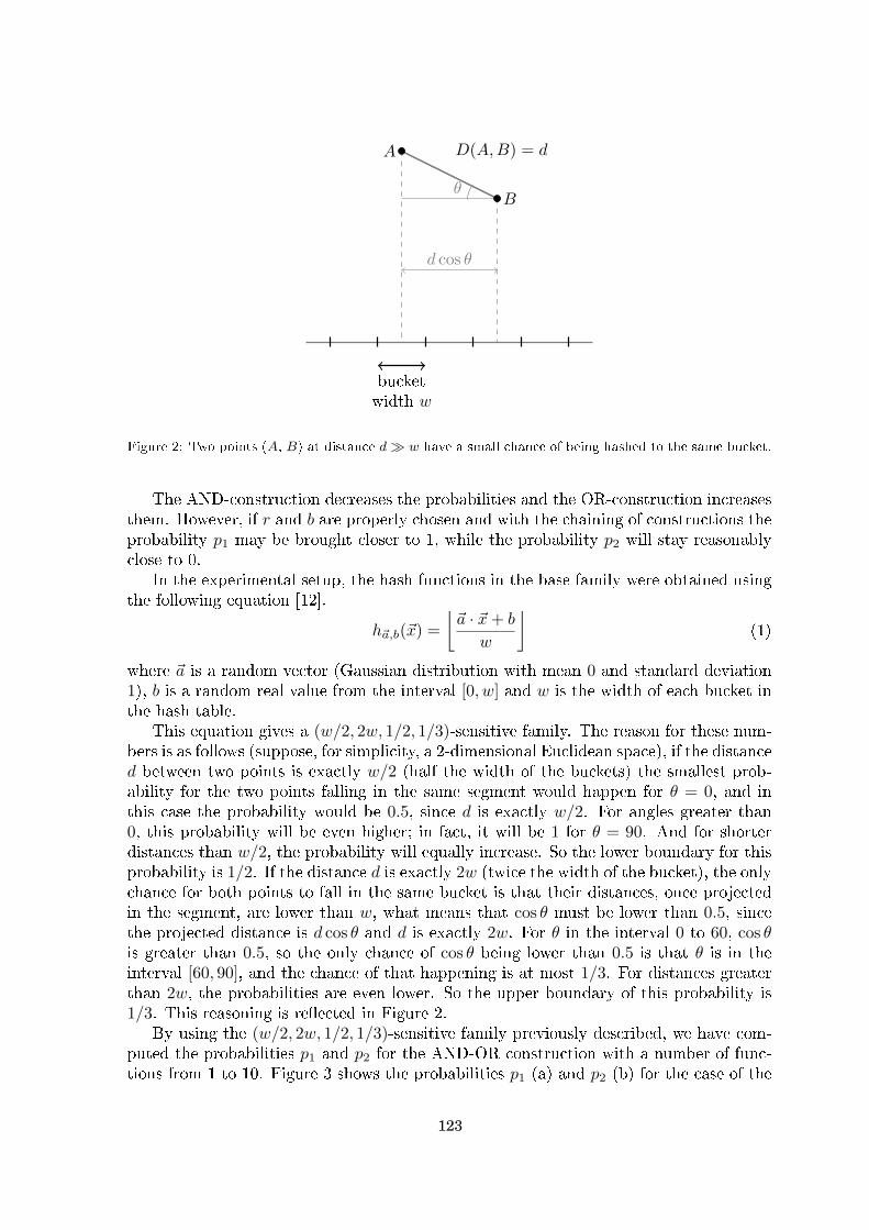
θ

d cos θ

A

B

D(A,B) = d

bucketwidth w

Figure 2: Two points (A, B) at distance d� w have a small chance of being hashed to the same bucket.

The AND-construction decreases the probabilities and the OR-construction increasesthem. However, if r and b are properly chosen and with the chaining of constructions theprobability p1 may be brought closer to 1, while the probability p2 will stay reasonablyclose to 0.

In the experimental setup, the hash functions in the base family were obtained usingthe following equation [12].

h~a,b(~x) =

⌊~a · ~x+ b

w

⌋(1)

where ~a is a random vector (Gaussian distribution with mean 0 and standard deviation1), b is a random real value from the interval [0, w] and w is the width of each bucket inthe hash table.

This equation gives a (w/2, 2w, 1/2, 1/3)-sensitive family. The reason for these num-bers is as follows (suppose, for simplicity, a 2-dimensional Euclidean space), if the distanced between two points is exactly w/2 (half the width of the buckets) the smallest prob-ability for the two points falling in the same segment would happen for θ = 0, and inthis case the probability would be 0.5, since d is exactly w/2. For angles greater than0, this probability will be even higher; in fact, it will be 1 for θ = 90. And for shorterdistances than w/2, the probability will equally increase. So the lower boundary for thisprobability is 1/2. If the distance d is exactly 2w (twice the width of the bucket), the onlychance for both points to fall in the same bucket is that their distances, once projectedin the segment, are lower than w, what means that cos θ must be lower than 0.5, sincethe projected distance is d cos θ and d is exactly 2w. For θ in the interval 0 to 60, cos θis greater than 0.5, so the only chance of cos θ being lower than 0.5 is that θ is in theinterval [60, 90], and the chance of that happening is at most 1/3. For distances greaterthan 2w, the probabilities are even lower. So the upper boundary of this probability is1/3. This reasoning is re�ected in Figure 2.

By using the (w/2, 2w, 1/2, 1/3)-sensitive family previously described, we have com-puted the probabilities p1 and p2 for the AND-OR construction with a number of func-tions from 1 to 10. Figure 3 shows the probabilities p1 (a) and p2 (b) for the case of the

123

0.500

0.750

0.875

0.938

0.969

0.984

0.992

0.996

0.998

0.999

0.250

0.438

0.578

0.684

0.763

0.822

0.867

0.900

0.925

0.944

0.125

0.234

0.330

0.414

0.487

0.551

0.607

0.656

0.699

0.737

0.062

0.121

0.176

0.228

0.276

0.321

0.363

0.403

0.441

0.476

0.031

0.062

0.091

0.119

0.147

0.173

0.199

0.224

0.249

0.272

0.016

0.031

0.046

0.061

0.076

0.090

0.104

0.118

0.132

0.146

0.008

0.016

0.023

0.031

0.038

0.046

0.053

0.061

0.068

0.075

0.004

0.008

0.012

0.016

0.019

0.023

0.027

0.031

0.035

0.038

0.002

0.004

0.006

0.008

0.010

0.012

0.014

0.016

0.017

0.019

0.001

0.002

0.003

0.004

0.005

0.006

0.007

0.008

0.009

0.010

1 2 3 4 5 6 7 8 9 10

1

2

3

4

5

6

7

8

9

10

0.1

0.2

0.3

0.4

0.5

0.6

0.7

0.8

0.9

(a) p1

0.300

0.510

0.657

0.760

0.832

0.882

0.918

0.942

0.960

0.972

0.090

0.172

0.246

0.314

0.376

0.432

0.483

0.530

0.572

0.611

0.027

0.053

0.079

0.104

0.128

0.151

0.174

0.197

0.218

0.239

0.008

0.016

0.024

0.032

0.040

0.048

0.055

0.063

0.071

0.078

0.002

0.005

0.007

0.010

0.012

0.014

0.017

0.019

0.022

0.024

0.001

0.001

0.002

0.003

0.004

0.004

0.005

0.006

0.007

0.007

0.000

0.000

0.001

0.001

0.001

0.001

0.002

0.002

0.002

0.002

0.000

0.000

0.000

0.000

0.000

0.000

0.000

0.001

0.001

0.001

0.000

0.000

0.000

0.000

0.000

0.000

0.000

0.000

0.000

0.000

0.000

0.000

0.000

0.000

0.000

0.000

0.000

0.000

0.000

0.000

1 2 3 4 5 6 7 8 9 10

1

2

3

4

5

6

7

8

9

10

0.1

0.2

0.3

0.4

0.5

0.6

0.7

0.8

0.9

(b) p2

0.200

0.240

0.218

0.178

0.137

0.102

0.075

0.054

0.038

0.027

0.160

0.266

0.332

0.369

0.387

0.390

0.383

0.370

0.353

0.333

0.098

0.181

0.251

0.310

0.359

0.400

0.433

0.460

0.481

0.497

0.054

0.105

0.152

0.196

0.236

0.273

0.308

0.340

0.370

0.397

0.029

0.057

0.084

0.110

0.135

0.159

0.182

0.205

0.227

0.248

0.015

0.030

0.044

0.058

0.072

0.086

0.099

0.113

0.126

0.138

0.008

0.015

0.023

0.030

0.037

0.045

0.052

0.059

0.066

0.073

0.004

0.008

0.011

0.015

0.019

0.023

0.027

0.030

0.034

0.038

0.002

0.004

0.006

0.008

0.010

0.012

0.013

0.015

0.017

0.019

0.001

0.002

0.003

0.004

0.005

0.006

0.007

0.008

0.009

0.010

1 2 3 4 5 6 7 8 9 10

1

2

3

4

5

6

7

8

9

10

0.05

0.1

0.15

0.2

0.25

0.3

0.35

0.4

0.45

(c) p1 − p2

Figure 3: Probabilities p1 and p2 and the di�erence between them. The darker the color the higherthe value. Each cell gives the value for the chaining of an OR-construction (number of combined basicfunctions on the x-axis) after an AND-construction (on the y-axis the number of combined functions).

chaining of an OR-construction just after an AND-construction, and the di�erence be-tween these two probabilities (c). The row number indicates the number of functions usedin the AND-construction, while the column number indicates the number of functionsused in the OR-construction.

4. New instance selection algorithms based on hashing

This section presents the algorithms proposed in this work: LSH-IS-S and LSH-IS-F. The �rst completes the selection process in a single pass, analyzing each instanceconsecutively. It processes instances in one pass, so not all instances need to �t inmemory. The second performs two passes: in the initial one, it counts the instances ineach bucket, in the second, it completes the instance selection with this information. Thecomplexity of both algorithms is linear, O(n) (note that this is even true for the secondalgorithm, i.e. although two passes are performed).

Both algorithms can be seen as incremental methods, due to the fact that the selecteddata set is formed by successive additions to the empty set. However, the second oneconforms more closely to batch processing because it analyzes the impact of the removalon the whole data set.

The main advantage of the presented methods is the drastic reduction in executiontime. The experimental results show a signi�cant di�erence when they are comparedagainst state-of-the-art instance selection algorithms.

4.1. LSH-IS-S: One-pass processing

As shown in Algorithm 1, the inputs of the LSH-IS-S method are: a set of instancesto select and a set of families of hash functions. The loop processes each instance x of X,using the function families to determine the bucket u to which the instance belongs3. Ifin the bucket u assigned to the instance there is no other instance of the same class of x,

3The bucket identi�er u given to an instance by a family g ∈ G can be thought of as the concatenationof all bucket identi�ers given by the hash functions in g, since the function families in G are obtainedby using an AND-construction on base functions obtained using Equation 1. The OR-construction isimplemented in the foreach loop at line 3 of Algorithm 1.

124

x is selected and added to S and to the bucket u. The algorithm ends when all instancesin X have been processed. Note that each instance is processed only once, which grantsan extremely fast performance at the expense of not analyzing the instances that areselected in each bucket in detail. Instances are analyzed in sequence without needinginformation on other instances. This process means that the method may be used in asingle-pass process, without requiring the whole dataset to �t in the memory.

Algorithm 1: LSH-IS-S � Instance selection algorithm by hashing in one pass.

Input: A training set X = {(x1, y1), ..., (xn, yn)}, set G of hash function familiesOutput: The set of selected instances S ⊆ X

1 S = ∅2 foreach instance x ∈ X do

3 foreach function family g ∈ G do4 u← bucket assigned to x by family g5 if there is no other instance of the same class of x in u then6 Add x to S7 Add x to u

8 return S

4.2. LSH-IS-F: A more informed selection

The algorithm explained in the previous section is remarkably fast and allows in-stances to be processed as they arrive, in one pass. On the other hand, because of how itworks, it is not using all information that may be relevant to decide which instances tochoose. For example, the algorithm has no control over the number of instances of eachclass that go to each bucket, because once an instance of a class is selected, it discardsother instances of the same class that may come later.

LSH-IS-F (see Algorithm 2) is an evolution of the LSH-IS-S. In this method, one-passprocessing is replaced by a more informed selection. The �rst loop is similar to LSH-IS-S but, instead of directly selecting instances, it �rst records the bucket to which eachinstance belongs. When there is only one instance of a class, the instance is rejected,otherwise, if two or more instances of the same class are present, one of them is randomlychosen. The idea here is to give the algorithm some tolerance of the presence of noise inthe input data set.

The execution time of this method is not much larger than in the previous method,since the number of buckets is much lower than the number of instances. Although, thedi�erences in execution time increase with the increase in the number of OR functions.

4.3. Behavior of proposed methods

The aim of this section is to try to shed some light on the behavior of the new al-gorithms proposed in the paper. As previously stated, LSH-IS-S makes the selectionof instances in one pass, selecting one instance of each class in each bucket. On theother hand, LSH-IS-F tries to avoid retaining noisy instances. The more informed se-lection criterion of LSH-IS-F allows it to remove instances that can be harmful for theclassi�cation.

125

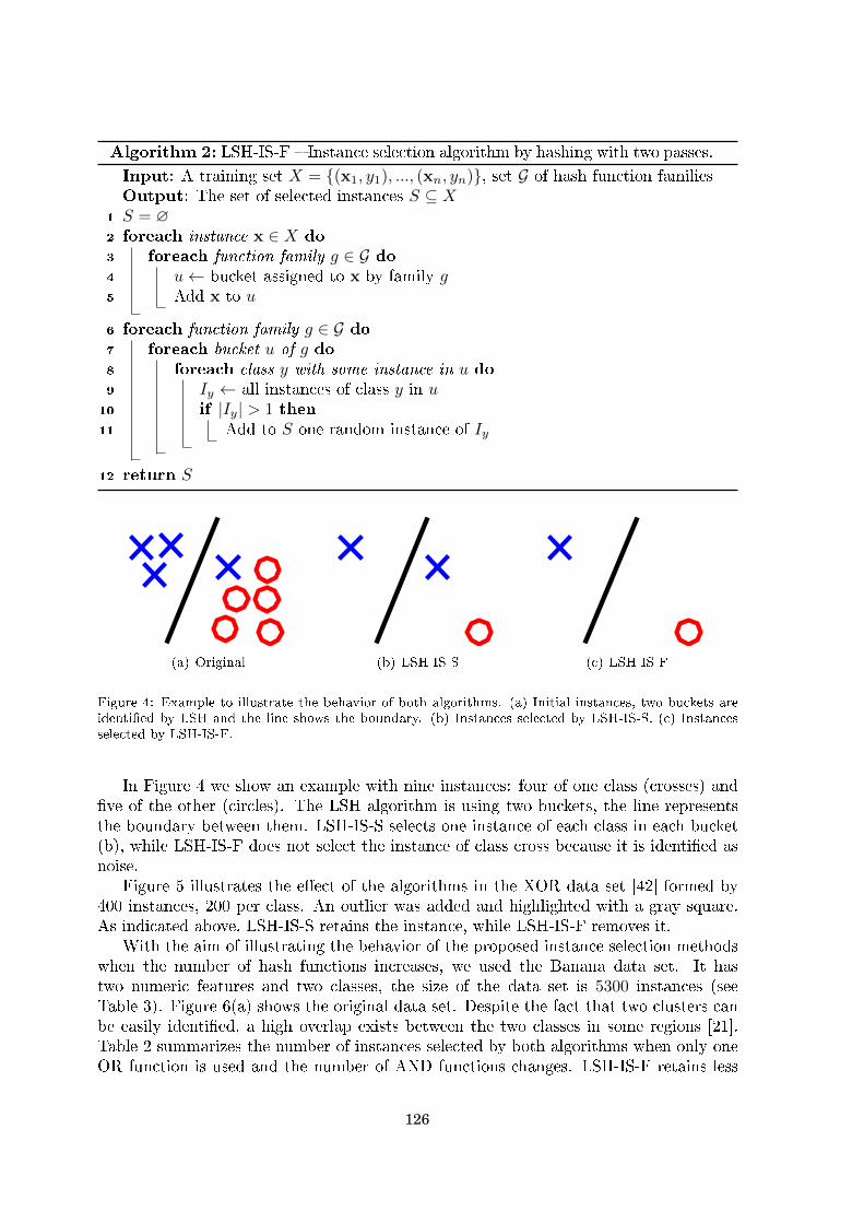
Algorithm 2: LSH-IS-F � Instance selection algorithm by hashing with two passes.

Input: A training set X = {(x1, y1), ..., (xn, yn)}, set G of hash function familiesOutput: The set of selected instances S ⊆ X

1 S = ∅2 foreach instance x ∈ X do

3 foreach function family g ∈ G do4 u← bucket assigned to x by family g5 Add x to u

6 foreach function family g ∈ G do7 foreach bucket u of g do8 foreach class y with some instance in u do9 Iy ← all instances of class y in u10 if |Iy| > 1 then11 Add to S one random instance of Iy

12 return S

(a) Original (b) LSH-IS-S (c) LSH-IS-F

Figure 4: Example to illustrate the behavior of both algorithms. (a) Initial instances, two buckets areidenti�ed by LSH and the line shows the boundary. (b) Instances selected by LSH-IS-S. (c) Instancesselected by LSH-IS-F.

In Figure 4 we show an example with nine instances: four of one class (crosses) and�ve of the other (circles). The LSH algorithm is using two buckets, the line representsthe boundary between them. LSH-IS-S selects one instance of each class in each bucket(b), while LSH-IS-F does not select the instance of class cross because it is identi�ed asnoise.

Figure 5 illustrates the e�ect of the algorithms in the XOR data set [42] formed by400 instances, 200 per class. An outlier was added and highlighted with a gray square.As indicated above, LSH-IS-S retains the instance, while LSH-IS-F removes it.

With the aim of illustrating the behavior of the proposed instance selection methodswhen the number of hash functions increases, we used the Banana data set. It hastwo numeric features and two classes, the size of the data set is 5300 instances (seeTable 3). Figure 6(a) shows the original data set. Despite the fact that two clusters canbe easily identi�ed, a high overlap exists between the two classes in some regions [21].Table 2 summarizes the number of instances selected by both algorithms when only oneOR function is used and the number of AND functions changes. LSH-IS-F retains less

126

(a) Original (b) LSH-IS-S (c) LSH-IS-F

Figure 5: (a) Original XOR example, an outlier is highlighted in gray. (b) LSH-IS-S selection maintainsthe outlier. (c) LSH-IS-F removes the outlier.

Table 2: Number of Banana data set instances that the proposed algorithms retain by the number ofAND functions.

Algorithm Number of AND functions

2 4 6 8 10

LSH-IS-S 25 123 249 466 684LSH-IS-F 24 110 225 423 627

instances, because those instances of one class isolated in one bucket with instances ofthe other class are ident�ed as noise and therefore deleted.

Figures 6 and 7 show the instances retained by both algorithms, LSH-IS-S and LSH-IS-F respectively, when only one OR function is used and di�erent numbers of ANDfunctions: 2, 4, 6, 8 and 10. The number of retained instances increases with the numberof functions. This behavior is quite interesting, because it enables the user to choosewhether more or fewer instances are retained, by varying the number of functions thatare used.

5. Experimental study

This section presents the experimental study performed to evaluate the new proposedmethods. We compared them against seven well-known state-of-the-art instance selectionalgorithms in a study performed in Weka [62]. The instance selection methods includedin the experiments were: CNN, ICF, MSS, DROP3, PSC, HMN-EI, LSBo and the twoapproaches based on hashing. The parameters selected for the algorithms were thoserecommended by the authors: the number of nearest neighbors used on ICF and DROP3were set to k = 3, the number of clusters for PSC was set to 6r (where r is the number ofclasses of the data set). Evolutionary algorithms were not included in the experiments,due to their high computational cost.

For the experiments, we used 30 data sets from the Keel repository [1] that haveat least 1000 instances. Table 3 summarizes the data sets: name, number of features,number of instances and the accuracy given by two classi�ers (using ten fold cross-validation): the nearest neighbor classi�er with k = 1 and the J48, a classi�er tree (the

127

-3 -2 -1 0 1 2 3-3

-2

-1

0

1

2

3

(a) Banana (Orig.)

-3 -2 -1 0 1 2 3-3

-2

-1

0

1

2

3

(b) LSH-IS-S: AND=2

-3 -2 -1 0 1 2 3-3

-2

-1

0

1

2

3

(c) LSH-IS-S: AND=4

-3 -2 -1 0 1 2 3-3

-2

-1

0

1

2

3

(d) LSH-IS-S: AND=6

-3 -2 -1 0 1 2 3-3

-2

-1

0

1

2

3

(e) LSH-IS-S: AND=8

-3 -2 -1 0 1 2 3-3

-2

-1

0

1

2

3

(f) LSH-IS-S: AND=10

Figure 6: The number of instances selected by LSH-IS-S as the number of functions increases.

-3 -2 -1 0 1 2 3-3

-2

-1

0

1

2

3

(a) Banana (Orig.)

-3 -2 -1 0 1 2 3-3

-2

-1

0

1

2

3

(b) LSH-IS-F: AND=2

-3 -2 -1 0 1 2 3-3

-2

-1

0

1

2

3

(c) LSH-IS-F: AND=4

-3 -2 -1 0 1 2 3-3

-2

-1

0

1

2

3

(d) LSH-IS-F: AND=6

-3 -2 -1 0 1 2 3-3

-2

-1

0

1

2

3

(e) LSH-IS-F: AND=8

-3 -2 -1 0 1 2 3-3

-2

-1

0

1

2

3

(f) LSH-IS-F: AND=10

Figure 7: The number of instances selected by LSH-IS-F as the number of functions increases.

128

Weka implementation of C4.5 [53]). The last �ve data sets are huge (below dashed line),with more than 299 000 instances, the traditional instance selection methods are unableto address them. The only transformation carried out was the normalization of all inputfeatures, to set their values at between 0 and 1.

We used the nearest neighbor classi�er (1NN), as most instance selection methodshave been designed for that classi�er (k = 1 in kNN) [37, 51]. Moreover, we used the J48classi�er tree, to evaluate the extent to which the instances selected by the algorithmswere suitable for training other classi�ers.

As shown in Section 3, there are ways of combining the hash functions families thatappear more promising than others (see Figure 3). However, it is unclear which of themwill achieve the best results in combination with the proposed algorithms. Therefore,we conducted a study with 60 combinations: AND-constructions, combining between 1to 10 hash functions, and OR-constructions, combining 1 to 6 functions, obtained bythe previous AND-construction, avoiding constructions with too many functions and,consequently, reducing the computational cost.

The subsets selected by the algorithms were used to build a classi�er (1NN), theaverage rank [14] of which was performed over the accuracy of all 60 combinations.Average ranks were calculated as follows: the results of the experiments were sorted, onefor the best method, two for the second, and so on. In the case of a tie, values of the rankswere added up and divided into the number of methods that tied. When the ranking ofeach data set was calculated, the average for each method was computed. Better methodshad rankings closer to one. The results of the rankings are shown in Figure 8. Each cellrepresents the ranking value for a speci�c combination of AND-OR-constructions, wherethe number of functions in the OR-constructions is shown by the x-axis and the numberof functions in the AND-constructions is shown by the y-axis number. The darker thecell the higher its ranking (lower values are better). The best con�guration is di�erentfor each algorithm:

• LSH-IS-S: the best con�guration is one that uses OR-constructions of 6 functionsobtained using an AND-construction on 10 functions of the base family (functionsobtained using Equation 1).

• LSH-IS-F: the best results were obtained using OR-constructions of 5 functionsobtained by combining by AND-construction 10 functions of the base family.

Figure 9 shows how the time execution increases, on average, for the proposed algo-rithms: LSH-IS-S (gray) and LSH-IS-F (black). The higher the number of AND func-tions, the bigger the gap between LSH-IS-S and LSH-IS-F. This behavior is explainedbecause LSH-IS-F has one loop more than LSH-IS-S (see pseudocodes 1 and 2) that isused to go through all the buckets counting the number of instances of each class. Thenumber of buckets searched increases with the number of hash functions.

Ten fold cross-validation was applied to the instance selection methods under study.The performances were as follows:

• accuracy achieved by 1NN and J48 classi�ers trained with the selected subset;

• �ltering time by instance selection;

• reduction achieved by instance selection methods (size of the selected subset).

129

Table 3: Summary of data sets characteristics: name, number of features, number of instances andaccuracy (1NN). Last �ve data sets, below dashed line, are huge problems.

Data sets # attributes # instances Accuracy

Continuous Nominal 1NN J48

1 German 7 13 1 000 72.90 71.802 Flare 0 11 1 066 73.26 73.553 Contraceptive 9 0 1 473 42.97 53.224 Yeast 8 0 1 484 52.22 56.745 Wine-quality-red 11 0 1 599 64.85 62.046 Car 0 6 1 728 93.52 92.367 Titanic 3 0 2 201 79.06 79.068 Segment 19 0 2 310 97.23 96.629 Splice 0 60 3 190 74.86 94.1710 Chess 0 35 3 196 72.12 81.8511 Abalone 7 1 4 174 19.84 20.7212 Spam 0 57 4 597 91.04 92.9713 Wine-quality-white 11 0 4 898 65.40 58.2314 Banana 2 0 5 300 87.21 89.0415 Phoneme 5 0 5 404 90.19 86.4216 Page-blocks 10 0 5 472 95.91 97.0917 Texture 40 0 5 500 99.04 93.1318 Optdigits 63 0 5 620 98.61 90.6919 Mushroom 0 22 5 644 100.00 100.0020 Satimage 37 0 6 435 90.18 86.2821 Marketing 13 0 6 876 28.74 31.0622 Thyroid 21 0 7 200 92.35 99.7123 Ring 20 0 7 400 75.11 90.9524 Twonorm 20 0 7 400 94.81 85.1225 Coil 2000 85 0 9 822 90.62 93.9526 Penbased 16 0 10 992 99.39 96.5327 Nursery 0 8 12 960 98.13 97.1328 Magic 10 0 19 020 80.95 85.0129 Letter 16 0 20 000 96.04 87.9830 KR vs. K 0 6 28 058 73.05 56.58

31 Census 7 30 299 285 92.70 95.4232 KDDCup99 33 7 494 021 99.95 99.9533 CovType 54 0 581 012 94.48 94.6434 KDDCup991M 33 7 1 000 000 99.98 99.9835 Poker 5 5 1 025 010 50.61 68.25

130

58.015

54.000

49.970

43.864

38.030

36.242

32.530

29.682

26.879

24.182

56.030

49.939

45.152

37.712

30.742

27.424

23.652

20.636

18.303

17.136

54.030

47.742

40.303

32.106

28.636

25.924

21.167

18.636

16.091

14.712

53.091

46.121

41.091

32.167

27.545

24.273

20.167

16.439

14.788

13.212

52.197

44.667

35.333

30.242

24.848

21.652

17.409

14.288

12.818

11.667

51.682

43.348

33.848

29.727

24.197

20.727

15.833

13.288

12.333

11.530

1 2 3 4 5 6

1

2

3

4

5

6

7

8

9

1015

20

25

30

35

40

45

50

55

(a) LSH-IS-S

58.348

54.045

48.409

43.303

39.773

35.136

31.773

27.439

25.621

20.697

56.606

50.409

43.030

38.303

30.682

25.833

20.879

18.955

17.061

15.561

54.727

47.697

42.364

37.212

30.379

24.485

19.576

16.773

14.894

13.667

53.697

46.227

41.879

35.742

29.273

24.212

18.985

16.121

14.348

12.864

52.667

45.197

39.333

32.091

25.045

21.485

16.985

15.015

12.318

11.258

52.091

43.485

38.136

30.561

23.909

20.273

15.924

13.894

12.076

11.273

1 2 3 4 5 6

1

2

3

4

5

6

7

8

9

1015

20

25

30

35

40

45

50

55

(b) LSH-IS-F

Figure 8: Average rank over accuracy of the proposed methods for the di�erent con�gurations of AND-OR constructions. The darker the cell, the higher the ranking (lower is better). Each cell represents anAND-OR-construction where the column is the number of functions in the OR-construction and the rowis the number of functions in the AND-construction.

1 2 3 4 5 6 7 8 9 100

500

1000

1500

2000

2500

3000

3500

LSH-IS-F 6 ORs

LSH-IS-S 6 ORs

LSH-IS-F 5 ORs

LSH-IS-S 5 ORs

LSH-IS-F 4 ORs

LSH-IS-S 4 ORs

LSH-IS-F 3 ORs

LSH-IS-S 3 ORs

LSH-IS-F 2 ORs

LSH-IS-S 2 ORs

LSH-IS-F 1 ORs

LSH-IS-S 1 ORs

# AND functions

Tim

e (

ms)

Figure 9: Average execution time of the proposed algorithms as the number of AND-functions increases.LSH-IS-S is represented in gray and LSH-IS-F in black with di�erent lines and marks for the di�erentnumbers of OR-functions.

131

Table 4: Average ranks and Hochberg procedureover accuracy: 1NN.

Algorithm Ranking p Hoch.

HMN-EI 2.92LSBo 3.85 0.1869LSH-IS-F 4.45 0.0602MSS 4.58 0.0553LSH-IS-S 4.98 0.0139DROP3 5.03 0.0138CNN 5.17 0.0088ICF 5.75 0.0004PSC 8.27 0.0000

Table 5: Average ranks and Hochberg procedureover accuracy: J48.


LSH-IS-F 3.63LSH-IS-S 3.88 0.7237HMN-EI 4.10 0.7237LSBo 4.57 0.5606MSS 5.03 0.1909CNN 5.28 0.0981ICF 5.67 0.0242DROP3 5.90 0.0094PSC 6.93 0.0000

Table 6: Average ranks and Hochberg procedure over storage reduction, and average reduction rate.

Algorithm Ranking p Hoch. Reduction rate

DROP3 1.67 0.896ICF 3.10 0.0427 0.813LSBo 3.70 0.0081 0.737PSC 4.70 0.0001 0.762CNN 5.43 0.0000 0.658MSS 6.00 0.0000 0.665HMN-EI 6.10 0.0000 0.577LSH-IS-F 6.62 0.0000 0.455LSH-IS-S 7.68 0.0000 0.405

According to the accuracy of 1NN classi�er (see Table 4), the best four algorithmswere HMN-EI followed by LSBo, LSH-IS-F and MSS. According to the Hochberg pro-cedure [29], di�erences between them were not signi�cant at a 0.05 signi�cance level.However, di�erences between LSBo and the other methods were signi�cant. When J48was used as the classi�er (see Table 5), the best six algorithms were LSH-IS-F followedby LSH-IS-S, HMN-EI, LSBo, MSS and CNN; the di�erences between them were notsigni�cant at 0.05. Furthermore, as can be seen, the least accurate model is PSC forboth classi�ers.

Table 6 shows the average ranks over compression. DROP3 is the best method at a0.05 signi�cance level. Furthermore, the average reduction rate for each method is alsoshown. The proposed methods are the most conservative, although, as previously stated,a higher compression could have been achieved using fewer functions in the LSH process.

The third relevant feature of instance selection methods is the time required by thealgorithms to calculate the selected subset. Table 7 shows the average rank over executiontime of the instance selection algorithms. The three fastest methods were LSH-IS-F, LSH-IS-S and PSC, between them di�erences were not signi�cant at a 0.05 signi�cance level.The di�erences were signi�cant from MSS and the following methods; the slowest was

132

Table 7: Average ranks and Hochberg procedure over �ltering time.


LSH-IS-F 1.53LSH-IS-S 1.57 0.9624PSC 3.00 0.0761MSS 4.20 0.0005ICF 5.33 0.0000LSBo 6.73 0.0000HMN-EI 6.70 0.0000DROP3 7.67 0.0000CNN 8.27 0.0000

CNN. It is worth noting that PSC achieved, according to the signi�cance tests, a reallycompetitive execution time. Nevertheless the shortcoming of PSC was its poor accuracy,as it obtained the worst results of all of the methods under analysis, as noted in Tables 4and 5.

It might be surprising that LSH-IS-F was faster than LSH-IS-S, because this contra-dicts Figure 9. The reason for this was the number of functions used by the algorithms;as commented on at the beginning of this section, LSH-IS-S was launched using 6 ORfunctions, while LSH-IS-F was launched with only 5.

Figure 10 shows the �ltering time as a function of the number of instances. Theresults obtained with the data sets of the experiments were used to draw these �gures.Since there were no results available for all possible values of numbers of instances, theavailable results were used to draw Bezier lines and to show the general trend of thealgorithms. Although other methods (CNN, HMN-EI, LSBo, DROP3, MSS and ICF)have an execution time that increases swiftly, our algorithms based on hashing are at thebottom of the �gures together with PSC. However, in the logarithmic scale, the growthof PSC is visibly greater.

As a summary of the experimentation with medium size data sets, we can highlightthat the proposed methods achieved competitive results in terms of accuracy. Consideringthe reduction rate, DROP3 achieved the maximum compression, while our methods werethe worst in terms of compression. Finally, considering execution time, the methodspresented in the paper were able to compute the selected subset much faster than theother algorithms in the state of the art. Exceptionally, PSC worked surprisingly fast,although slower than the speed of our proposals, and with the shortcoming of the pooraccuracy when its selected subsets were used for training the classi�ers.

5.1. Huge problems

Due to the fact that instance selection methods are not able to face huge problems,the experimental study performed over Census, CovType, KDDCup99, KDDCup991M4

4We divided the original KDDCup 1999 data set into two sets with di�erent number of instances:KDDCup99 has 10% of the original instances and KDDCup991M has a million.

133

0 0.2 0.4 0.6 0.8 1 1.2 1.4 1.6 1.8 2

Number of instances #10 4

0

0.5

1

1.5

2

2.5

3

3.5

4

4.5

5

Tim

e (m

s)

#10 5

DROP3-bDROP3HMNEI-bHMNEIICF-bICFLSBo-bLSBoMSS-bMSSPSC-bPSCLSH-IS-S-bLSH-IS-SLSH-IS-F-bLSH-IS-F

(a) Linear scale

0 0.2 0.4 0.6 0.8 1 1.2 1.4 1.6 1.8 2

Number of instances #10 4

10 0

10 1

10 2

10 3

10 4

10 5

10 6

10 7

10 8

Tim

e (m

s)

CNN-bCNNDROP3-bDROP3HMNEI-bHMNEIICF-bICFLSBo-bLSBoMSS-bMSSPSC-bPSCLSH-IS-S-bLSH-IS-SLSH-IS-F-bLSH-IS-F

(b) Logarithmic scale

Figure 10: Computational cost of tested methods, in linear (a) and logarithmic scale (b) on the y axis.In (a) the CNN was not plotted because its growth was so high that it was not possible to appreciatethe di�erences between the other methods. The dots are the results on the available data sets, lines(denoted by �-b� in the legend) are the Bezier lines built with these dots to show the general trend ofthe algorithms.

134

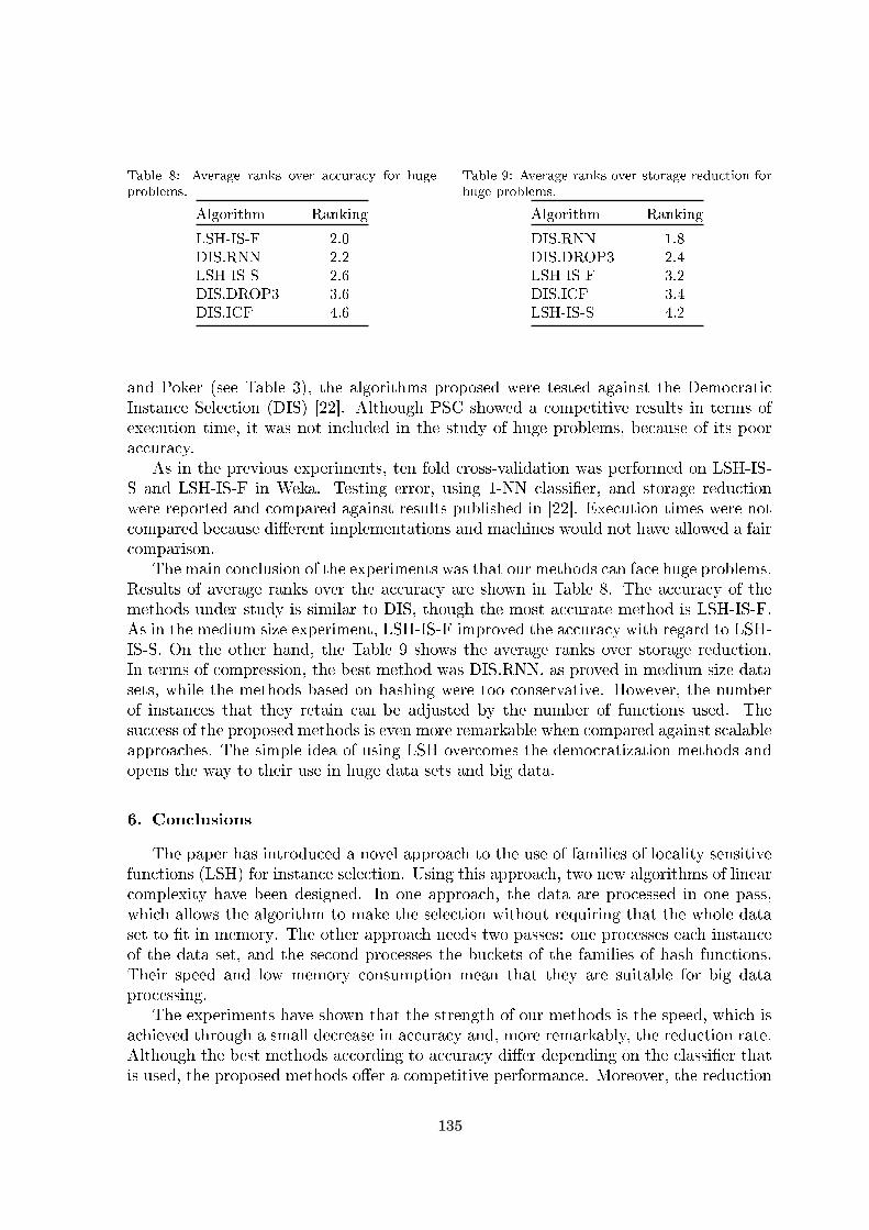
Table 8: Average ranks over accuracy for hugeproblems.

Algorithm Ranking

LSH-IS-F 2.0DIS.RNN 2.2LSH-IS-S 2.6DIS.DROP3 3.6DIS.ICF 4.6

Table 9: Average ranks over storage reduction forhuge problems.

Algorithm Ranking

DIS.RNN 1.8DIS.DROP3 2.4LSH-IS-F 3.2DIS.ICF 3.4LSH-IS-S 4.2

and Poker (see Table 3), the algorithms proposed were tested against the DemocraticInstance Selection (DIS) [22]. Although PSC showed a competitive results in terms ofexecution time, it was not included in the study of huge problems, because of its pooraccuracy.

As in the previous experiments, ten fold cross-validation was performed on LSH-IS-S and LSH-IS-F in Weka. Testing error, using 1-NN classi�er, and storage reductionwere reported and compared against results published in [22]. Execution times were notcompared because di�erent implementations and machines would not have allowed a faircomparison.

The main conclusion of the experiments was that our methods can face huge problems.Results of average ranks over the accuracy are shown in Table 8. The accuracy of themethods under study is similar to DIS, though the most accurate method is LSH-IS-F.As in the medium size experiment, LSH-IS-F improved the accuracy with regard to LSH-IS-S. On the other hand, the Table 9 shows the average ranks over storage reduction.In terms of compression, the best method was DIS.RNN, as proved in medium size datasets, while the methods based on hashing were too conservative. However, the numberof instances that they retain can be adjusted by the number of functions used. Thesuccess of the proposed methods is even more remarkable when compared against scalableapproaches. The simple idea of using LSH overcomes the democratization methods andopens the way to their use in huge data sets and big data.

6. Conclusions

The paper has introduced a novel approach to the use of families of locality sensitivefunctions (LSH) for instance selection. Using this approach, two new algorithms of linearcomplexity have been designed. In one approach, the data are processed in one pass,which allows the algorithm to make the selection without requiring that the whole dataset to �t in memory. The other approach needs two passes: one processes each instanceof the data set, and the second processes the buckets of the families of hash functions.Their speed and low memory consumption mean that they are suitable for big dataprocessing.

The experiments have shown that the strength of our methods is the speed, which isachieved through a small decrease in accuracy and, more remarkably, the reduction rate.Although the best methods according to accuracy di�er depending on the classi�er thatis used, the proposed methods o�er a competitive performance. Moreover, the reduction

135

rate can be adjusted by increasing or by decreasing the number of hash functions thatare used.

Furthermore, the proposed methods were evaluated on huge problems and comparedagainst Democratic Instance Selection, a linear complexity method. Experimental resultson accuracy showed how our methods outperformed DIS, even though our methods wereconceptually much simpler.

7. Future work

In their current version, the way the algorithms make the instance selection is verysimple and quite �naive�. The selected subset could be improved using additional infor-mation about the instances assigned to each bucket, and not just the count of instancesof each class. A future research line could be to store additional information of the in-stances assigned to each bucket: for example, simple statistics such as the incrementalaverage of instances in the bucket, or the percentage of instances of each class in thebucket. This information might mean that the instance selection process would be bet-ter informed, without excessively penalizing run-time. Although prototype generationhas not been analyzed in the paper, the generation of a new instance, or group of them,for each bucket is one of the future lines of research. This idea can be developed usingLSH-IS-F, seeking each of the buckets to build or to create a new set of instances, byselecting the medoids or centroids of the instances in the buckets.

According to [63], one of the most challenging problems in data mining research ismining data streams in extremely large databases. Accurate and fast processes able towork on stream are required, without any assumption that information can be storedin large databases and repeatedly accessed. One of the problems that arises in thoseenvironments is called concept drift, which appears when changes in the context takeplace. In the management of concept drift, three basic approaches can be distinguished:ensemble learning, instance weighting and instance selection [59]. A comparison of theproposed method in a streaming benchmark would be made to test whether LSH-IS-Scan beat the state-of-the-art algorithms that are able to deal in streaming data [18].

Many more research approaches can be considered, but the principal one for us is toadapt the new methods to a big data environment. We are working on the adaptationof this idea to a MapReduce framework, which o�ers a robust environment to face up tothe processing of huge data sets over clusters of machines [58].

Acknowledgements

Supported by the Research Projects TIN 2011-24046 and TIN 2015-67534-P from theSpanish Ministry of Economy and Competitiveness.

References

[1] Jesus Alcalá-Fdez, Luciano Sánchez, Salvador Garcia, M.Jose del Jesus, Sebastián Ventura, J.M.Garrell, Jose Otero, Cristóbal Romero, Jaume Bacardit, Victor M. Rivas, J.C. Fernández, andFrancisco Herrera. Keel: a software tool to assess evolutionary algorithms for data mining problems.Soft Computing, 13(3):307�318, 2009.

136

[2] Álvar Arnaiz-González, José F. Díez-Pastor, Juan J. Rodríguez, and César Ignacio García-Osorio.Instance selection for regression by discretization. Expert Systems with Applications, 54:340 � 350,2016.

[3] Alexandr Andoni and Piotr Indyk. Near-optimal hashing algorithms for approximate nearest neigh-bor in high dimensions. Commun. ACM, 51(1):117�122, January 2008.

[4] Sunil Arya, David M. Mount, Nathan S. Netanyahu, Ruth Silverman, and Angela Y. Wu. An optimalalgorithm for approximate nearest neighbor searching �xed dimensions. J. ACM, 45(6):891�923,November 1998.

[5] Daniel Asimov. The grand tour: A tool for viewing multidimensional data. SIAM J. Sci. Stat.Comput., 6(1):128�143, January 1985.

[6] Ricardo Barandela, Francesc J. Ferri, and José Salvador Sánchez. Decision boundary preservingprototype selection for nearest neighbor classi�cation. IJPRAI, 19(6):787�806, 2005.

[7] Henry Brighton and Chris Mellish. On the consistency of information �lters for lazy learningalgorithms. In JanM. �ytkow and Jan Rauch, editors, Principles of Data Mining and KnowledgeDiscovery, volume 1704 of Lecture Notes in Computer Science, pages 283�288. Springer BerlinHeidelberg, 1999.

[8] Henry Brighton and Chris Mellish. Advances in instance selection for instance-based learningalgorithms. Data Mining and Knowledge Discovery, 6(2):153�172, 2002.

[9] Jorge Calvo-Zaragoza, Jose J. Valero-Mas, and Juan R. Rico-Juan. Improving kNN multi-labelclassi�cation in prototype selection scenarios using class proposals. Pattern Recognition, 48(5):1608� 1622, 2015.

[10] José Ramón Cano, Francisco Herrera, and Manuel Lozano. Strati�cation for scaling up evolutionaryprototype selection. Pattern Recognition Letters, 26(7):953 � 963, 2005.

[11] T. Cover and P. Hart. Nearest neighbor pattern classi�cation. Information Theory, IEEE Trans-actions on, 13(1):21�27, January 1967.

[12] Mayur Datar, Nicole Immorlica, Piotr Indyk, and Vahab S. Mirrokni. Locality-sensitive hashingscheme based on p-stable distributions. In Proceedings of the Twentieth Annual Symposium onComputational Geometry, SCG '04, pages 253�262, New York, NY, USA, 2004. ACM.

[13] Aida de Haro-García and Nicolás García-Pedrajas. A divide-and-conquer recursive approach forscaling up instance selection algorithms. Data Mining and Knowledge Discovery, 18(3):392�418,2009.

[14] Janez Dem²ar. Statistical comparisons of classi�ers over multiple data sets. J. Mach. Learn. Res.,7:1�30, December 2006.

[15] Joaquín Derrac, Salvador García, and Francisco Herrera. Strati�ed prototype selection based on asteady-state memetic algorithm: a study of scalability. Memetic Computing, 2(3):183�199, 2010.

[16] Joaquín Derrac, Salvador García, and Francisco Herrera. A survey on evolutionary instance selectionand generation. Int. J. Appl. Metaheuristic Comput., 1(1):60�92, January 2010.

[17] Joaquín Derrac, Nele Verbiest, Salvador García, Chris Cornelis, and Francisco Herrera. On theuse of evolutionary feature selection for improving fuzzy rough set based prototype selection. SoftComputing, 17(2):223�238, 2013.

[18] Gregory Ditzler, Manuel Roveri, Cesare Alippi, and Robi Polikar. Learning in nonstationary envi-ronments: A survey. Computational Intelligence Magazine, IEEE, 10(4):12�25, 2015.

[19] F. Dornaika and I. Kamal Aldine. Decremental sparse modeling representative selection for proto-type selection. Pattern Recognition, 48(11):3714 � 3727, 2015.

[20] Richard O Duda, Peter E Hart, and David G Stork. Pattern classi�cation. John Wiley & Sons,2012.

[21] Salvador Garcia, Joaquín Derrac, J.Ramón Cano, and Francisco Herrera. Prototype selection fornearest neighbor classi�cation: Taxonomy and empirical study. Pattern Analysis and MachineIntelligence, IEEE Transactions on, 34(3):417�435, March 2012.

[22] César García-Osorio, Aida de Haro-García, and Nicolás García-Pedrajas. Democratic instanceselection: A linear complexity instance selection algorithm based on classi�er ensemble concepts.Arti�cial Intelligence, 174(5-6):410�441, 2010.

[23] Nicolás García-Pedrajas and Aida de Haro-García. Boosting instance selection algorithms.Knowledge-Based Systems, 67:342 � 360, 2014.

[24] Nicolás García-Pedrajas, Juan Antonio Romero del Castillo, and Domingo Ortiz-Boyer. A coopera-tive coevolutionary algorithm for instance selection for instance-based learning. Machine Learning,78(3):381�420, 2010.

[25] G. Gates. The reduced nearest neighbor rule (corresp.). Information Theory, IEEE Transactionson, 18(3):431�433, May 1972.

137

[26] Alberto Guillen, L.Javier Herrera, Ginés Rubio, Héctor Pomares, Amaury Lendasse, and IgnacioRojas. New method for instance or prototype selection using mutual information in time seriesprediction. Neurocomputing, 73(10�12):2030 � 2038, 2010. Subspace Learning / Selected papersfrom the European Symposium on Time Series Prediction.

[27] P. Hart. The condensed nearest neighbor rule (corresp.). Information Theory, IEEE Transactionson, 14(3):515 � 516, may 1968.

[28] Pablo Hernandez-Leal, J.Ariel Carrasco-Ochoa, J.Francisco Martínez-Trinidad, and J.ArturoOlvera-López. Instance rank based on borders for instance selection. Pattern Recognition, 46(1):365� 375, 2013.

[29] Yosef Hochberg. A sharper bonferroni procedure for multiple tests of signi�cance. Biometrika,75(4):800�802, 1988.

[30] Piotr Indyk and Rajeev Motwani. Approximate nearest neighbors: Towards removing the curse ofdimensionality. In Proceedings of the Thirtieth Annual ACM Symposium on Theory of Computing,STOC '98, pages 604�613, New York, NY, USA, 1998. ACM.

[31] Norbert Jankowski and Marek Grochowski. Comparison of instances seletion algorithms I. algo-rithms survey. In Leszek Rutkowski, J orgH. Siekmann, Ryszard Tadeusiewicz, and Lot�A. Zadeh,editors, Arti�cial Intelligence and Soft Computing - ICAISC 2004, volume 3070 of Lecture Notesin Computer Science, pages 598�603. Springer Berlin Heidelberg, 2004.

[32] S.-W. Kim and John B. Oommen. A brief taxonomy and ranking of creative prototype reductionschemes. Pattern Analysis & Applications, 6(3):232�244, 2003.

[33] Mirosªaw Kordos, Szymon Biaªka, and Marcin Blachnik. Instance selection in logical rule extrac-tion for regression problems. In Leszek Rutkowski, Marcin Korytkowski, Rafaª Scherer, RyszardTadeusiewicz, Lot� A. Zadeh, and Jacek M. Zurada, editors, Arti�cial Intelligence and Soft Com-puting, volume 7895 of Lecture Notes in Computer Science, pages 167�175. Springer Berlin Heidel-berg, 2013.

[34] Eyal Kushilevitz, Rafail Ostrovsky, and Yuval Rabani. E�cient search for approximate nearestneighbor in high dimensional spaces. In Proceedings of the Thirtieth Annual ACM Symposium onTheory of Computing, STOC '98, pages 614�623, New York, NY, USA, 1998. ACM.

[35] Jure Leskovec, Anand Rajaraman, and Je�rey David Ullman. Mining of Massive Datasets. Cam-bridge University Press, 2nd edition, 2014.

[36] Enrique Leyva, Antonio González, and Raúl Pérez. Knowledge-based instance selection: A com-promise between e�ciency and versatility. Knowledge-Based Systems, 47:65 � 76, 2013.

[37] Enrique Leyva, Antonio González, and Raúl Pérez. Three new instance selection methods based onlocal sets: A comparative study with several approaches from a bi-objective perspective. PatternRecognition, 48(4):1523 � 1537, 2015.

[38] Juan Li and Yuping Wang. A new fast reduction technique based on binary nearest neighbor tree.Neurocomputing, 149, Part C:1647 � 1657, 2015.

[39] Ting Liu, Andrew W Moore, Ke Yang, and Alexander G Gray. An investigation of practicalapproximate nearest neighbor algorithms. In Advances in neural information processing systems,pages 825�832. MIT Press, 2004.

[40] Alessandra Lumini and Loris Nanni. A clustering method for automatic biometric template selec-tion. Pattern Recognition, 39(3):495 � 497, 2006.

[41] Elena Marchiori. Hit miss networks with applications to instance selection. J. Mach. Learn. Res.,9:997�1017, June 2008.

[42] Elena Marchiori. Class conditional nearest neighbor for large margin instance selection. IEEETransactions on Pattern Analysis and Machine Intelligence, 32(2):364�370, Feb 2010.

[43] Emanuela Merelli, Marco Pettini, and Mario Rasetti. Topology driven modeling: the is metaphor.Natural Computing, 14(3):421�430, 2014.

[44] C. Moretti, K. Steinhaeuser, D. Thain, and N. V. Chawla. Scaling up classi�ers to cloud computers.In Data Mining, 2008. ICDM '08. Eighth IEEE International Conference on, pages 472�481, Dec2008.

[45] Loris Nanni and Alessandra Lumini. Prototype reduction techniques: A comparison among di�erentapproaches. Expert Systems with Applications, 38(9):11820 � 11828, 2011.

[46] J.Arturo Olvera-López, J.Ariel Carrasco-Ochoa, and J.Francisco Martínez-Trinidad. A new fastprototype selection method based on clustering. Pattern Analysis and Applications, 13(2):131�141,2009.

[47] J.Arturo Olvera-López, J.Francisco Martínez-Trinidad, J.Ariel Carrasco-Ochoa, and Josef Kittler.Prototype selection based on sequential search. Intelligent Data Analysis, 13(4):599�631, 2009.

[48] Stefanos Ougiaroglou, Georgios Evangelidis, and Dimitris A Dervos. FHC: an adaptive fast hybrid

138

method for k-NN classi�cation. Logic Journal of the IGPL, 2015.[49] Daniel Peralta, Sara del Río, Sergio Ramírez-Gallego, Isaac Triguero, Jose M Benitez, and Fran-

cisco Herrera. Evolutionary feature selection for big data classi�cation: A mapreduce approach.Mathematical Problems in Engineering, 501:246139, 2015.

[50] JA Pérez-Benítez, JL Pérez-Benítez, and JH Espina-Hernández. Novel data condensing methodusing a prototype's front propagation algorithm. Engineering Applications of Arti�cial Intelligence,39:181�197, 2015.

[51] Javier Pérez-Rodríguez, Alexis Germán Arroyo-Peña, and Nicolás García-Pedrajas. Simultaneousinstance and feature selection and weighting using evolutionary computation: Proposal and study.Applied Soft Computing, 37:416 � 443, 2015.

[52] El»bieta P¦kalska, Robert P.W. Duin, and Pavel Paclík. Prototype selection for dissimilarity-based classi�ers. Pattern Recognition, 39(2):189 � 208, 2006. Part Special Issue: ComplexityReductionPart Special Issue: Complexity Reduction.

[53] J. Ross Quinlan. C4.5: Programs for Machine Learning. Morgan Kaufmann Publishers Inc., SanFrancisco, CA, USA, 1993.

[54] GL Ritter, HB Woodru�, SR Lowry, and TL Isenhour. An algorithm for a selective nearest neighbordecision rule. IEEE Transactions on Information Theory, 21(6):665�669, 1975.

[55] Milo² B. Stojanovi¢, Milo² M. Boºi¢, Milena M. Stankovi¢, and Zoran P. Staji¢. A methodology fortraining set instance selection using mutual information in time series prediction. Neurocomputing,141:236 � 245, 2014.

[56] Hung Tran-The, Vinh Nguyen Van, and Minh Hoang Anh. Fast approximate near neighbor al-gorithm by clustering in high dimensions. In Knowledge and Systems Engineering (KSE), 2015Seventh International Conference on, pages 274�279, Oct 2015.

[57] Isaac Triguero, Joaquín Derrac, Salvador Garcia, and Francisco Herrera. A taxonomy and ex-perimental study on prototype generation for nearest neighbor classi�cation. Systems, Man, andCybernetics, Part C: Applications and Reviews, IEEE Transactions on, 42(1):86�100, 2012.

[58] Isaac Triguero, Daniel Peralta, Jaume Bacardit, Salvador García, and Francisco Herrera. MRPR:A mapreduce solution for prototype reduction in big data classi�cation. Neurocomputing, 150, PartA:331 � 345, 2015.

[59] Alexey Tsymbal. The problem of concept drift: de�nitions and related work. Computer ScienceDepartment, Trinity College Dublin, 106:2, 2004.

[60] D. Randall Wilson and Tony R. Martinez. Instance pruning techniques. In Machine Learning:Proceedings of the Fourteenth International Conference (ICML'97), pages 404�411. Morgan Kauf-mann, 1997.

[61] D. Randall Wilson and Tony R. Martinez. Reduction techniques for instance-based learning algo-rithms. Machine Learning, 38(3):257�286, March 2000.

[62] Ian H. Witten, Eibe Frank, and Mark A. Hall. Data Mining: Practical Machine Learning Toolsand Techniques. Morgan Kaufmann Publishers Inc., San Francisco, CA, USA, 3rd edition, 2011.

[63] Qiang Yang and Xindong Wu. 10 challenging problems in data mining research. InternationalJournal of Information Technology & Decision Making, 05(04):597�604, 2006.

139

BIBLIOGRAPHY

Aha, D. W., Kibler, D., and Albert, M. K. (1991).

Instance-based learning algorithms.

Machine Learning, 6(1):37–66.

Angiulli, F. and Folino, G. (2007).

Distributed nearest neighbor-based condensation of very large data sets.

Knowledge and Data Engineering, IEEE Transactions on, 19(12):1593–1606.

Appice, A. and Džeroski, S. (2007).

Stepwise induction of multi-target model trees.

In Proceedings of the 18th European Conference on Machine Learning, ECML ’07, pages

502–509, Berlin, Heidelberg. Springer-Verlag.

Arnaiz-González, Á., Blachnik, M., Kordos, M., and García-Osorio, C. (2016).

Fusion of instance selection methods in regression tasks.

Information Fusion, 30:69 – 79.

Arnaiz-González, Á., Díez-Pastor, J. F., Rodríguez, J. J., and García-Osorio, C. I. (2016a).

Instance selection for regression: Adapting DROP.

Neurocomputing, 201:66 – 81.

Arnaiz-González, Á., Díez-Pastor, J. F., Rodríguez, J. J., and García-Osorio, C. I. (2016b).

Instance selection for regression by discretization.

Expert Systems with Applications, 54:340 – 350.

Arnaiz-González, Á., Díez-Pastor, J. F., Rodríguez, J. J., and García-Osorio, C. I. (2016c).

Instance selection of linear complexity for big data.

Knowledge-Based Systems, 107:83 – 95.

Baeza Yates, R. A. and Neto, B. R. (1999).

Modern Information Retrieval.

Addison-Wesley Longman Publishing Co., Inc., Boston, MA, USA.

Barandela, R., Ferri, F. J., and Sánchez, J. S. (2005).

Decision boundary preserving prototype selection for nearest neighbor classification.

141

BIBLIOGRAPHY

IJPRAI, 19(6):787–806.

Barandela, R., Sánchez, J., García, V., and Rangel, E. (2003).

Strategies for learning in class imbalance problems.

Pattern Recognition, 36(3):849 – 851.

Brighton, H. and Mellish, C. (2002).

Advances in instance selection for instance-based learning algorithms.

Data Mining and Knowledge Discovery, 6(2):153–172.

Cano, J. R., Herrera, F., and Lozano, M. (2005a).

Stratification for scaling up evolutionary prototype selection.

Pattern Recognition Letters, 26(7):953 – 963.

Cano, J. R., Herrera, F., and Lozano, M. (2005b).

A Study on the Combination of Evolutionary Algorithms and Stratified Strategies for Training

Set Selection in Data Mining, pages 271–284.

Springer Berlin Heidelberg, Berlin, Heidelberg.

Charte, F., Rivera, A. J., del Jesus, M. J., and Herrera, F. (2014).

MLeNN: A first approach to heuristic multilabel undersampling.

In Intelligent Data Engineering and Automated Learning – IDEAL 2014: 15th International

Conference, Salamanca, Spain, September 10-12, 2014. Proceedings, pages 1–9, Cham. Springer

International Publishing.

Chawla, N. V., Hall, L. O., Bowyer, K. W., and Kegelmeyer, W. P. (2004).

Learning ensembles from bites: A scalable and accurate approach.

Journal of Machine Learning Research, 5:421–451.

Collberg, C. and Proebsting, T. A. (2016).

Repeatability in computer systems research.

Communications ACM, 59(3):62–69.

Cover, T. and Hart, P. (1967).

Nearest neighbor pattern classification.

Information Theory, IEEE Transactions on, 13(1):21–27.

de Haro-García, A. and García-Pedrajas, N. (2009).

A divide-and-conquer recursive approach for scaling up instance selection algorithms.


Dean, J. and Ghemawat, S. (2008).

MapReduce: Simplified data processing on large clusters.

Communications ACM, 51(1):107–113.

142

BIBLIOGRAPHY

Demšar, D., Džeroski, S., Larsen, T., Struyf, J., Axelsen, J., Pedersen, M. B., and Krogh, P. H.

(2006).

Using multi-objective classification to model communities of soil microarthropods.

Ecological Modelling, 191(1):131 – 143.

Selected Papers from the Fourth International Workshop on Environmental Applications of

Machine Learning, September 27 - October 1, 2004, Bled, Slovenia.

Derrac, J., García, S., Molina, D., and Herrera, F. (2011).

A practical tutorial on the use of nonparametric statistical tests as a methodology for comparing

evolutionary and swarm intelligence algorithms.

Swarm and Evolutionary Computation, 1(1):3 – 18.

Devroye, L., Györfi, L., and Lugosi, G. (1996).

A Probabilistic Theory of Pattern Recognition.

Springer Verlag.

Garcia, S., Derrac, J., Cano, J., and Herrera, F. (2012).

Prototype selection for nearest neighbor classification: Taxonomy and empirical study.

Pattern Analysis and Machine Intelligence, IEEE Transactions on, 34(3):417–435.

García, S., Luengo, J., and Herrera, F. (2014).

Data Preprocessing in Data Mining.

Springer Publishing Company, Incorporated.

García, S., Luengo, J., and Herrera, F. (2016).

Tutorial on practical tips of the most influential data preprocessing algorithms in data mining.


García, S., Ramírez-Gallego, S., Luengo, J., Benítez, J. M., and Herrera, F. (2016).

Big data preprocessing: methods and prospects.

Big Data Analytics, 1(1):9.

García-Osorio, C., de Haro-García, A., and García-Pedrajas, N. (2010).

Democratic instance selection: A linear complexity instance selection algorithm based on

classifier ensemble concepts.

Artificial Intelligence, 174(5-6):410–441.

García-Pedrajas, N. and de Haro-García, A. (2014).

Boosting instance selection algorithms.


Gates, G. (1972).

The reduced nearest neighbor rule (corresp.).

143

BIBLIOGRAPHY

Information Theory, IEEE Transactions on, 18(3):431–433.

Guillen, A., Herrera, L., Rubio, G., Pomares, H., Lendasse, A., and Rojas, I. (2010).

New method for instance or prototype selection using mutual information in time series

prediction.

Neurocomputing, 73(10-12):2030 – 2038.

Han, J., Pei, J., and Kamber, M. (2011).

Data mining: concepts and techniques.

Elsevier.

Hart, P. (1968).

The condensed nearest neighbor rule (corresp.).

Information Theory, IEEE Transactions on, 14(3):515 – 516.

Iman, R. L. and Davenport, J. M. (1980).

Approximations of the critical region of the fbietkan statistic.

Communications in Statistics - Theory and Methods, 9(6):571–595.

Jankowski, N. and Grochowski, M. (2004).

Comparison of instances seletion algorithms I. algorithms survey.

In Rutkowski, L., Siekmann, J., Tadeusiewicz, R., and Zadeh, L. A., editors, Artificial Intelli-

gence and Soft Computing - ICAISC 2004, volume 3070 of Lecture Notes in Computer Science,

pages 598–603. Springer Berlin Heidelberg.

Kanj, S., Abdallah, F., Denœux, T., and Tout, K. (2016).

Editing training data for multi-label classification with the k-nearest neighbor rule.

Pattern Analysis and Applications, 19(1):145–161.

Kohavi, R. (1995).

A study of cross-validation and bootstrap for accuracy estimation and model selection.

In Proceedings of the 14th International Joint Conference on Artificial Intelligence - Volume 2,

IJCAI’95, pages 1137–1143, San Francisco, CA, USA. Morgan Kaufmann Publishers Inc.

Kordos, M. and Blachnik, M. (2012).

Instance selection with neural networks for regression problems.

In Proceedings of the 22nd international conference on Artificial Neural Networks and Machine

Learning - Volume Part II, ICANN’12, pages 263–270. Springer-Verlag, Berlin, Heidelberg.

Kuncheva, L. I. (2004).

Combining Pattern Classifiers: Methods and Algorithms.

Wiley.

144

BIBLIOGRAPHY

Laney, D. (2001).

3-d data management: controlling data volume, velocity and variety.

Technical report, META Group Research Note.

Leskovec, J., Rajaraman, A., and Ullman, J. D. (2014).

Mining of Massive Datasets.

Cambridge University Press, 2nd edition.

Leyva, E., González, A., and Pérez, R. (2015).

Three new instance selection methods based on local sets: A comparative study with several

approaches from a bi-objective perspective.

Pattern Recognition, 48(4):1523 – 1537.

Liu, H. and Motoda, H. (2002).

On issues of instance selection.


Marchiori, E. (2008).

Hit miss networks with applications to instance selection.

Journal of Machine Learning Research, 9:997–1017.

Mayer-Schönberger, V. and Cukier, K. (2013).

Big data: A revolution that will transform how we live, work, and think.

Houghton Mifflin Harcourt.

McLachlan, G., Do, K.-A., and Ambroise, C. (2005).

Analyzing microarray gene expression data, volume 422.

John Wiley & Sons.

Minelli, M., Chambers, M., and Dhiraj, A. (2012).

Big data, big analytics: emerging business intelligence and analytic trends for today’s businesses.

John Wiley & Sons, Inc.

Nanni, L. and Lumini, A. (2011).

Prototype reduction techniques: A comparison among different approaches.

Expert Systems with Applications, 38(9):11820 – 11828.

Olvera-López, J., Carrasco-Ochoa, J., and Martínez-Trinidad, J. (2009a).

A new fast prototype selection method based on clustering.

Pattern Analysis and Applications, 13(2):131–141.

Olvera-López, J. A., Carrasco-Ochoa, J. A., Martínez-Trinidad, J. F., and Kittler, J. (2010).

A review of instance selection methods.

Artificial Intelligence Review, 34(2):133–143.

145

BIBLIOGRAPHY

Olvera-López, J. A., Martínez-Trinidad, F. J., Carrasco-Ochoa, J. A., and Kittler, J. (2009b).

Prototype selection based on sequential search.

Intelligent Data Analysis, 13(4):599–631.

Pérez-Benítez, J., Pérez-Benítez, J., and Espina-Hernández, J. (2015).

Novel data condensing method using a prototype’s front propagation algorithm.

Engineering Applications of Artificial Intelligence, 39:181 – 197.

Polikar, R. (2006).

Ensemble based systems in decision making.

IEEE Circuits and Systems Magazine, 6(3):21–45.

Rico-Juan, J. R. and Iñesta, J. M. (2012).

New rank methods for reducing the size of the training set using the nearest neighbor rule.

Pattern Recognition Letters, 33(5):654 – 660.

Schaffer, C. (1994).

A conservation law for generalization performance.

In Cohen, W. W. and Hirsch, H., editors, Proceedings of the Eleventh International Machine

Learning Conference, pages 259–265. Rutgers University, New Brunswick, NJ.

Sheskin, D. J. (2003).

Handbook of parametric and nonparametric statistical procedures.

crc Press.

Si, L., Yu, J., Wu, W., Ma, J., Wu, Q., and Li, S. (2017).

Rmhc-mr: Instance selection by random mutation hill climbing algorithm with mapreduce in

big data.

Procedia Computer Science, 111(Supplement C):252 – 259.

The 8th International Conference on Advances in Information Technology.

Silva, D. A., Souza, L. C., and Motta, G. H. (2016).

An instance selection method for large datasets based on Markov Geometric Diffusion.

Data & Knowledge Engineering, 101:24 – 41.

Song, Y., Liang, J., Lu, J., and Zhao, X. (2017).

An efficient instance selection algorithm for k nearest neighbor regression.

Neurocomputing, 251(Supplement C):26 – 34.

Spyromitros-Xioufis, E., Tsoumakas, G., Groves, W., and Vlahavas, I. (2012).

Multi-label classification methods for multi-target regression.

arXiv preprint arXiv, 1211.

146

BIBLIOGRAPHY

Tomek, I. (1976).

An experiment with the edited nearest-neighbor rule.

Systems, Man, and Cybernetics, IEEE Transactions on, SMC-6(6):448–452.

Triguero, I., Peralta, D., Bacardit, J., García, S., and Herrera, F. (2014).

A combined MapReduce-windowing two-level parallel scheme for evolutionary prototype gener-

ation.

In 2014 IEEE Congress on Evolutionary Computation (CEC), pages 3036–3043.

Triguero, I., Peralta, D., Bacardit, J., García, S., and Herrera, F. (2015).

MRPR: A mapreduce solution for prototype reduction in big data classification.

Neurocomputing, 150, Part A:331 – 345.

Tsymbal, A. (2004).

The problem of concept drift: definitions and related work.

Computer Science Department, Trinity College Dublin, 106(2).

Valero-Mas, J. J., Calvo-Zaragoza, J., Rico-Juan, J. R., and Iñesta, J. M. (2016).

An experimental study on rank methods for prototype selection.

Soft Computing, pages 1–13.

White, T. (2009).

Hadoop: The Definitive Guide.

O’Reilly Media, Inc., 1st edition.

Wilson, D. L. (1972).

Asymptotic properties of nearest neighbor rules using edited data.

Systems, Man and Cybernetics, IEEE Transactions on, SMC-2(3):408–421.

Wilson, D. R. and Martinez, T. R. (1997).

Instance pruning techniques.

In Machine Learning: Proceedings of the fourteenth international conference (ICML’97), pages

404–411. Morgan Kaufmann.

Wilson, D. R. and Martinez, T. R. (2000).

Reduction techniques for instance-based learning algorithms.

Machine Learning, 38(3):257–286.

Zaharia, M., Chowdhury, M., Franklin, M. J., Shenker, S., and Stoica, I. (2010).

Spark: Cluster computing with working sets.

In Proceedings of the 2nd USENIX Conference on Hot Topics in Cloud Computing, HotCloud’10,

pages 10–10, Berkeley, CA, USA. USENIX Association.

147

estudio de métodos de selección de instancias -...

Documents