estimaciÓn del hidrograma de crecientes …de eficiencia de nash-sutcliffe que varió de 0.72 a...

739

Resumen

En este estudio se destaca la importancia del uso de precipi-tación estimada por radar, en la modelación hidrológica de caudales máximos en cuencas con pluviometría deficiente. El modelado hidrológico con precipitación estimada por radar toma en consideración, detalladamente, la variabili-dad espacial y temporal de la precipitación. El objetivo del presente estudio fue evaluar la simulación hidrológica de la cuenca del río Escondido en la estación hidrométrica 24290 (en Villa de Fuentes, Coahuila, México). El modelo hidroló-gico HEC-HMS fue utilizado para simular los caudales pico con datos de precipitación estimada por radar. La cuenca se ubica en una zona semidesértica con la característica de escurrimientos efímeros y eventos extraordinarios poco fre-cuentes registrados durante el periodo de medición (1932 a la fecha). Los eventos analizados fueron: 3 de junio del 2003, 29 de septiembre del 2006 y 5 de abril del 2004, que han sido los únicos importantes del periodo de disponibili-dad de datos de radar. Los datos de precipitación etapa IV del radar NEXRAD, ubicado en la base militar Launghlin, Texas, fueron adaptados al caso de estudio. Para evaluar los resultados se utilizaron los criterios gráficos y numéricos: comparación de hidrogramas de forma visual y el coeficien-te de Eficiencia de Nash-Sutcliffe (E). Los resultados obteni-dos fueron satisfactorios debido a valores de los coeficientes Eficiencia de Nash-Sutcliffe (E) iguales con 0.96 en la cali-bración y 0.91 en la validación del modelo.

Palabras clave: HEC-HMS, NEXRAD, Eficiencia de Nash-Sutcliffe (E).

AbstRAct

In this study, the importance of using radar-based rainfall estimation for the modeling of peak flow in poorly gauged basin is highlighted. The hydrological modeling with radar estimated rainfall, takes into account, detailedly, the spatial and temporal variability of the rainfall. The aim of this study was to evaluate the hydrologic simulation of the Escondido river Basin in the hydrometric station 24290 (in Villa de Fuentes, Coahuila, Mexico). The HEC-HMS hydrologic model was used to simulate peak flows using radar-estimated rainfall data. The basin is located in a semi-desert area with the characteristic of ephemeral runoffs and rare extraordinary events recorded during the measurement period (1932 to date). The events analyzed were: June 3, 2003, September 29, 2006 and April 5, 2004, which have been the only important ones of the period of radar data availability. The stage IV precipitation data of NEXRAD radar, located in the military base Launghlin, Texas, were adapted to this case study. To evaluate the results graphical and numerical criteria were used: comparison of hydrographs and the Nash-Sutcliffe efficiency coefficient (E). The results were satisfactory due to coefficient values of Nash-Sutcliffe Efficiency (E) equal with 0.96 in calibration and 0.91 in validation of the model.

Key words: HEC-HMS, NEXRAD, Nash-Sutcliffe Efficiency (E).

IntRoductIon

The scarcity of rainfall data is a problem faced by hydrologists in hydrological studies, particularly in hydrological modeling of a

watershed. Confidence in the results of the hydrologic modeling depends heavily on the availability of

ESTIMACIÓN DEL HIDROGRAMA DE CRECIENTES CON MODELACIÓN DETERMINÍSTICA Y PRECIPITACIÓN DERIVADA DE RADAR

ESTIMATION OF FLOOD HYDROGRAPH USING DETERMINISTIC MODELING AND WEATHER RADAR RAINFALL

Francisco Magaña-Hernández1*, Khalidou M. Bâ1, Víctor H. Guerra-Cobián2

1Facultad de Ingeniería, Centro Interamericano de Recursos del Agua, Universidad Autónoma del Estado de México. Cerro de Coatepec CU s/n. 50110. Toluca, México. 2Instituto de Inge-niería Civil de la UANL, Ciudad Universitaria. 66450. San Nicolás de los Garza, Nuevo León, México. ([email protected]).

*Autor responsable v Author for correspondence.Recibido: julio, 2013. Aprobado: octubre, 2013.Publicado como ARTÍCULO en Agrociencia 47: 739-752. 2013.

740

AGROCIENCIA, 16 de noviembre - 31 de diciembre, 2013

VOLUMEN 47, NÚMERO 8

IntRoduccIón

La escasez de datos de lluvia es una problemá-tica que enfrentan los hidrólogos en estudios hidrológicos, particularmente en la mode-

lación hidrológica de una cuenca. La confianza en los resultados de la modelación hidrológica depende en gran medida de la disponibilidad de información meteorológica, así como de caudales para calibrar y validar las modelaciones en un modelo hidrológico. Los datos de precipitación para aplicaciones hi-drológicas se obtienen de una escasa red de pluvió-metros como la única fuente confiable en la mode-lación hidrológica de una cuenca (Rosengaus, 1995). Las redes terrestres de medición de lluvia (pluvióme-tros y particularmente pluviógrafos) son escasas en tiempo y espacio, o inexistentes. Esta situación limita la toma de decisiones para administrar los recursos hídricos y dificulta el desarrollo de sistemas de alerta temprana para el control de inundaciones o el diseño de obras hidráulicas. Una alternativa para solucionar este problema es el uso de imágenes generadas por radar meteorológico para estimar las precipitaciones en tiempo real o casi real. El radar meteorológico fue desarrollado casi pa-ralelamente por ingleses y estadounidenses como un instrumento para detectar y ubicar la distancia de aeronaves enemigas (Atlas, 1990). El National Weather Service (NWS), agencia de la Administra-ción Nacional Oceánica y Atmosférica (NOAA), y otras agencias han desplegado una red de 160 rada-res meteorológicos de vigilancia continua, para la cobertura nacional en EE.UU. (Fulton et al., 1998, Xie et al., 2005). Estos radares se denominan WSR-88D (Weather Surveillance Radar-1988 Doppler), y se conocen con el nombre de NEXRAD (NEXt generation RADar). NEXRAD es una red de radares meteorológicos de alta resolución de tipo Doppler y producen estimaciones de precipitación con la ma-yor resolución espacial y temporal tradicionalmente disponibles para los modelos hidrológicos (Whiton et al., 1998). Ewen et al. (2000), Molnar y Julien (2000) y Hundecha y Bárdossy (2004) usaron diversos mo-delos hidrológicos para simular escurrimientos. Bâ et al. (2001) usaron el modelo CEQUEAU para ana-lizar el comportamiento hidrológico de los caudales de las cuencas de los ríos Amacuzac y San Jeróni-mo (México). En Alemania, Hundecha y Bárdossy

meteorological information as well as flows to calibrate and validate the hydrological model. The rainfall data for hydrological applications are obtained from a sparse network of rain gauges as the only reliable source in a basin hydrologic modeling (Rosengaus, 1995). The rain measuring terrestrial networks (rain gauges and particularly pluviographs) are rare in time and space, or nonexistent. This limits the decision-making for managing water resources and hinders the development of early warning systems for flood control or design of hydraulic works. An alternative to overcome this problem is the use of weather radar-generated images to estimate rainfall data in real-time or almost real. The weather radar was developed almost simultaneously by English and Americans as a tool to detect and locate enemy aircraft distance (Atlas, 1990). The National Weather Service (NWS), an agency of the National Oceanic and Atmospheric Administration (NOAA) and other agencies have deployed a network of 160 continuous monitoring weather radars for the U.S. national coverage (Fulton et al., 1998, Xie et al., 2005). These radars are called WSR-88D (Weather Surveillance Radar-1988 Doppler), and are known by the name of NEXRAD (NEXt generation RADar). NEXRAD is a high-resolution meteorological Doppler radar network, and produce precipitation estimates with the highest spatial and temporal resolution traditionally available for hydrological models (Whiton et al., 1998). Ewen et al. (2000), Molnar and Julien (2000) and Hundecha and Bárdossy (2004) used various models to simulate hydrologic runoffs. Bâ et al. (2001) used the CEQUEAU model to analyze the hydrologic behavior of flows in the river basins of Amacuzac and San Jerónimo (Mexico). In Germany, Hundecha and Bárdossy (2004) applied the conceptual rainfall runoff model HBV_IWS in 95 subbasins of the Rhine river, to model the effects of land use change on runoff. NEXRAD rainfall data are used in hydrologic modeling of peak flows (Bedient et al., 2003; Whiteaker et al., 2006). Thus, Bedient et al. (2000) used data from rain gauges and NEXRAD KHGX radar in the basin of Brays Bayou near Houston, Texas, to simulate peak flows with the HEC-1 model. These authors found that the model overestimated the peak flow with the radar data compared with rain gauge data. Di Luzio and Arnold (2004) used rainfall


741MAGAÑA-HERNÁNDEZ et al.

(2004) aplicaron el modelo conceptual lluvia escu-rrimiento HBV_IWS en 95 subcuencas del río Rin para modelar los efectos del cambio de uso del suelo en el escurrimiento. Datos de precipitación NEXRAD se usan en la modelación hidrológica de caudales máximos (Be-dient et al., 2003; Whiteaker et al., 2006). Así, Be-dient et al. (2000) usaron datos de precipitación de pluviómetros y del radar NEXRAD KHGX en la cuenca del Brays Bayou, cerca de Houston, Texas, para simular los caudales picos con el modelo HEC-1. Estos autores encontraron que el modelo sobrees-timó el caudal pico con los datos de radar en com-paración con los datos de pluviómetros. Di Luzio y Arnold (2004) usaron datos de precipitación de radar NEXRAD para modelar 24 tormentas, y aplicaron el modelo SWAT para simulaciones horarias en la cuenca del Blue River en Oklahoma, EE.UU. Para calibrar el modelo usaron un método automático y un procedimiento manual, el cual sobreestimó los caudales pico para eventos de corta duración. Para evaluar las simulaciones, se basaron en el coeficiente de Eficiencia de Nash-Sutcliffe que varió de 0.72 a 0.90. El objetivo de la presente investigación fue simu-lar los caudales pico de la cuenca del río Escondido, Coahuila, México, con precipitación estimada por el radar NEXRAD KDFX, así como la calibración y va-lidación del modelo hidrológico HEC-HMS.

mAteRIAles y métodos

Zona en estudio

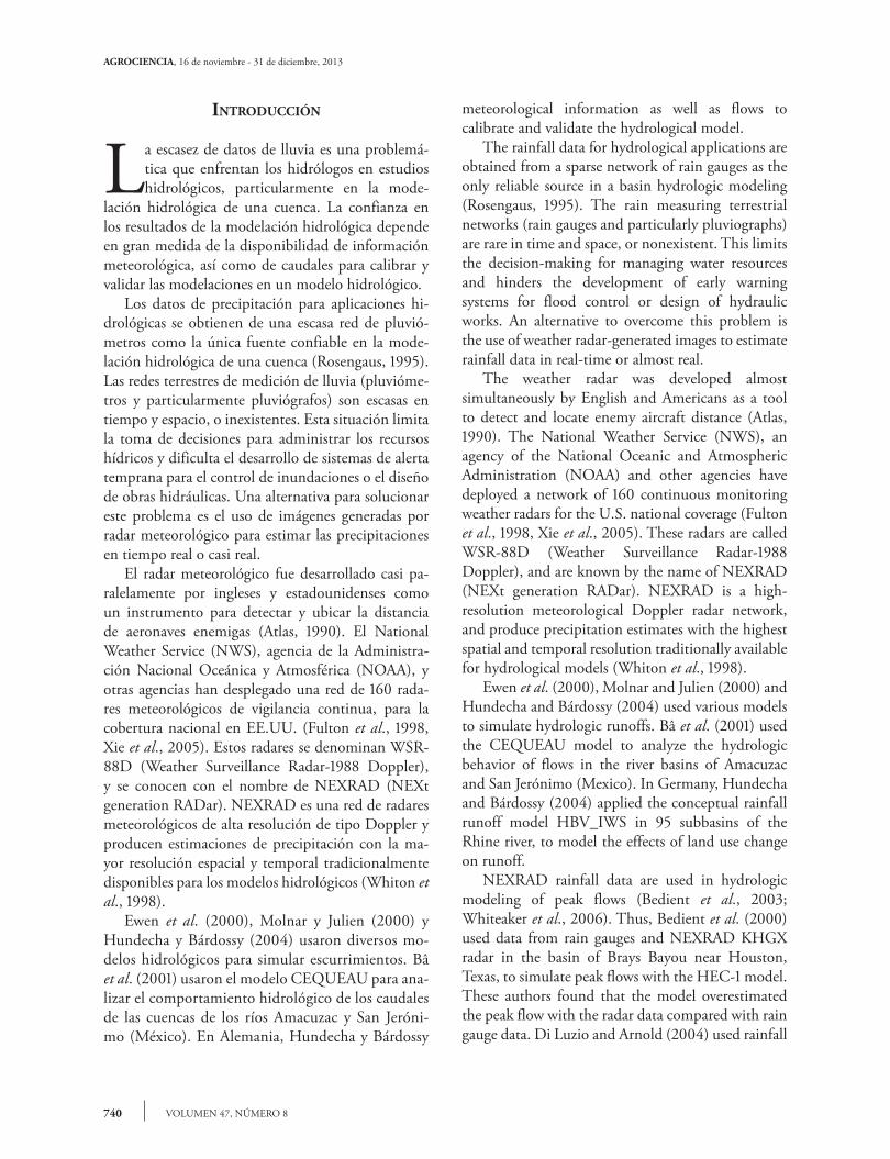
El río Escondido nace en la Sierra El Burro, al noroeste de la ciudad de Piedras Negras, Coahuila, México. La cuenca se loca-liza en una región semidesértica drenando un área de 3242 km2 hasta la estación hidrométrica Villa de Fuentes (Figura 1). La co-rriente principal se origina a una altitud de 1000 m y recorre una distancia de 155 km hasta alcanzar una altitud de 245 m donde se ubica la estación hidrométrica. En esta región, las lluvias son de tipo convectivo, asociadas con frentes fríos y ocasionalmente con eventos ciclónicos. Existen estaciones meteorológicas en la cuenca y se ubican en la desembocadura (Figura 1). La estación meteorológica Santa Cecilia fue instalada en 2004 después de la fuerte inundación que ocurrió en abril de dicho año. En esta situación de escasez de datos meteorológicos, fue necesario para este estudio usar datos del radar NEXRAD KDFX de la NOAA de EE.UU., disponibles desde el 2002 y el radio de cobertura del

data from NEXRAD radar to model 24 storms, and applied the SWAT model to time simulations in the Blue river basin in Oklahoma, USA. To calibrate the model an automatic method and a manual procedure was used, which overestimated peak flows for short events. The evaluation of simulations was based on the Nash-Sutcliffe efficiency coefficient and this varied between 0.72 and 0.90. The aim of this research was to simulate peak flows of the Escondido river basin, Coahuila, Mexico, with estimated rainfall by the NEXRAD KDFX radar, and the calibration and validation of hydrological model HEC-HMS.

mAteRIAls And methods

Study area

Escondido river rises in the Sierra El Burro, northwest of the city of Piedras Negras, Coahuila, Mexico. The basin is located in a semi-desert region draining an area of 3242 km2 to Villa de Fuentes hydrometric station (Figure 1). The main streamflow originates at an altitude of 1000 m and covers a distance of 155 km to reach an altitude of 245 m where hydrometric station is located. In this region, rainfall is convective, associated with cold fronts and with cyclonic events occasionally. There are weather stations in the basin and are located in the mouth of the river (Figure 1). The Santa Cecilia weather station was installed in 2004 following the heavy flooding that occurred in April that year. In this situation of scarcity of meteorological data, it was necessary for this study to use data of the NEXRAD KDFX radar from NOAA U.S.A. available since 2002 and the radius of the radar coverage completely covers the basin. These data were acquired for the period 2002-2008. In addition, there is hydrometric information on hourly level obtained from the International Boundary and Water Commission (IBWC). The files generated by the radar are binary and consist of a list of values precipitation in millimeters (Reed and Maidemt, 1999), which form a square grid known as HRAP (Hydrologic Rainfall Analysis Project). The radar data were processed using the Idrisi Taiga software and a code was developed to automate the processing of precipitation using Idrisi tools.

Hydrologic modeling

To perform the hydrological simulations the model HEC-HMS (HEC-2010) was used, where the modeling of the runoff production function is based on the Curve Number

742



radar cubre completamente la cuenca. Estos datos fueron adqui-ridos para el periodo de 2002 a 2008. Además, hay información hidrométrica horaria obtenida de la Comisión Internacional de Límites y Agua (CILA). Los archivos generados por el radar son de tipo binario y consisten en un listado de valores de precipi-tación en milímetros (Reed y Maidemt, 1999), que forman una malla de cuadros conocida como HRAP (Hydrologic Rainfall Analysis Project). Los datos de radar se procesaron con el Software Idrisi Taiga y se desarrolló un código para automatizar el procesamiento de la precipitación utilizando las herramientas de Idrisi.

Modelación hidrológica

Para realizar las simulaciones hidrológicas se empleó el modelo HEC-HMS (HEC-2010), donde la modelación de la función de producción del escurrimiento se basa en el método del Número de Curva (CN) del Servicio de Conservación de Suelos (SCS-CN). Este método se usa para predecir volumen de escurrimiento directo para un evento de lluvia dado. Fue desarrollado por el Departamento de Agricultura de EE.UU., del Servicio de Conservación de Suelos y documentado en de-talle en el Manual Nacional de Ingeniería, Secc. 4: Hidrología (NEH-4) (SCS, 1956, 1964, 1971, 1985, 1993). El método SCS-CN se basa en la ecuación de balance de agua. Este método en HEC-HMS estima la precipitación en exceso o precipitación efectiva en función de la precipitación acumulada, cobertura

(CN) method of the Soil Conservation Service (SCS-CN). This method is used for prediction of direct runoff volume for a given rainfall event. It was developed by the U.S. Department of Agriculture, the Soil Conservation Service and documented in detail in the National Engineering Manual, Sec. 4: Hydrology (NEH-4) (SCS, 1956, 1964, 1971, 1985, 1993). The SCS-CN method is based on the water balance equation. This method in HEC-HMS estimates the excess precipitation or effective precipitation as a function of cumulative precipitation, soil cover, land use, and antecedent moisture, as shown by Equation 1:

PP

CN

PCN

e =− +

+ −

508050 8

20320203 20

2.

. (1)

where Pe is excess rainfall (mm), P is accumulated precipitation (mm), CN is curve number that depends on the soil-use and type that exists in the basin.

The main weak points of SCS-CN are: it does not consider the impact of the rainfall intensity and its temporary distribution, it does not address the effects of the spatial scale, it is very sensitive to changes in the values of CN, and it clearly does not address the effect of adjacent moisture condition (Hawkins, 1993, Ponce and Hawkins, 1996, Michel et al., 2005).

Figura 1. Zona de estudio.Figure 1. Study area.



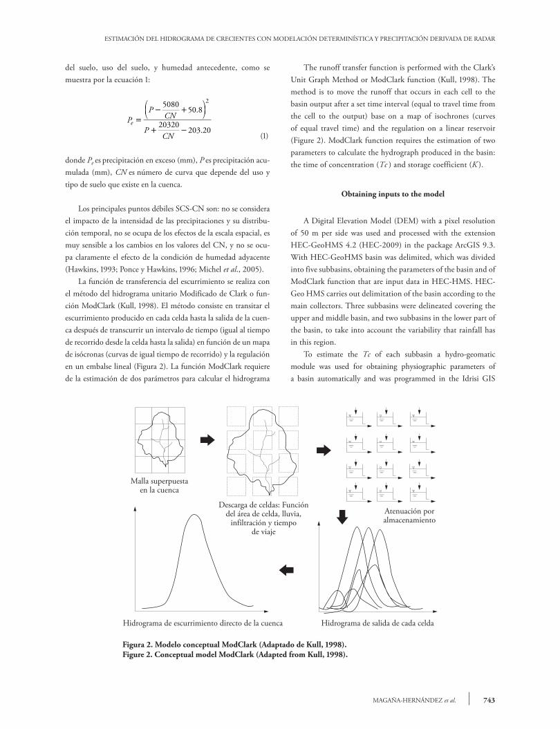
Figura 2. Modelo conceptual ModClark (Adaptado de Kull, 1998).Figure 2. Conceptual model ModClark (Adapted from Kull, 1998).

del suelo, uso del suelo, y humedad antecedente, como se muestra por la ecuación 1:

PP

CN

PCN

e =− +

+ −

508050 8

20320203 20

2.

. (1)

donde Pe es precipitación en exceso (mm), P es precipitación acu-mulada (mm), CN es número de curva que depende del uso y tipo de suelo que existe en la cuenca.

Los principales puntos débiles SCS-CN son: no se considera el impacto de la intensidad de las precipitaciones y su distribu-ción temporal, no se ocupa de los efectos de la escala espacial, es muy sensible a los cambios en los valores del CN, y no se ocu-pa claramente el efecto de la condición de humedad adyacente (Hawkins, 1993; Ponce y Hawkins, 1996; Michel et al., 2005). La función de transferencia del escurrimiento se realiza con el método del hidrograma unitario Modificado de Clark o fun-ción ModClark (Kull, 1998). El método consiste en transitar el escurrimiento producido en cada celda hasta la salida de la cuen-ca después de transcurrir un intervalo de tiempo (igual al tiempo de recorrido desde la celda hasta la salida) en función de un mapa de isócronas (curvas de igual tiempo de recorrido) y la regulación en un embalse lineal (Figura 2). La función ModClark requiere de la estimación de dos parámetros para calcular el hidrograma

The runoff transfer function is performed with the Clark’s Unit Graph Method or ModClark function (Kull, 1998). The method is to move the runoff that occurs in each cell to the basin output after a set time interval (equal to travel time from the cell to the output) base on a map of isochrones (curves of equal travel time) and the regulation on a linear reservoir (Figure 2). ModClark function requires the estimation of two parameters to calculate the hydrograph produced in the basin: the time of concentration (Tc ) and storage coefficient (K ).

Obtaining inputs to the model

A Digital Elevation Model (DEM) with a pixel resolution of 50 m per side was used and processed with the extension HEC-GeoHMS 4.2 (HEC-2009) in the package ArcGIS 9.3. With HEC-GeoHMS basin was delimited, which was divided into five subbasins, obtaining the parameters of the basin and of ModClark function that are input data in HEC-HMS. HEC-Geo HMS carries out delimitation of the basin according to the main collectors. Three subbasins were delineated covering the upper and middle basin, and two subbasins in the lower part of the basin, to take into account the variability that rainfall has in this region. To estimate the Tc of each subbasin a hydro-geomatic module was used for obtaining physiographic parameters of a basin automatically and was programmed in the Idrisi GIS

744



(Quentin et al., 2007). The information used by the module includes: the MDE of the study area and a raster file of the basin. The coefficient K can be estimated from a hydrograph observed: it represents the ratio between the low volume the hydrograph after the second inflection point (recession curve) and the value of spending on this point (HEC, 1982). The equation to estimate this coefficient is:

K

Q t

QdtPI

PI=

( )∞∫

(2)

where K is the storage coefficient, Q tPI( )∞∫ is the volume under

the hydrograph after the second point of inflection and QPI is the value of the spending on the inflection point.

The U.S.A. Army Corps of Engineers (HEC-1967) suggests that the storage coefficient K is equal to 0.8 times the concentration. Russell et al. (1979) found that KcTc and that this value varies from 1.5 to 2.8. According to Dominguez et al. (2008), for practical purposes the coefficient K can be estimated as the sixth of Tc. In this study, the initial value of K for each subbasin was estimated as half the Tc (K0.5Tc), and then this parameter should be calibrated. To obtain a raster image of the curve number CN vector maps were used of soil type and use of the National Institute of Statistics, Geography and Informatics (INEGI) scale 1:50 000. A reclassification of the soil type map was performed according to its hydrologic group, based on the soil classification of the U.S. Department of Agriculture (USDA) and then, through cartographical algebra in ArcGIS 9.3, the matrix image from CN was obtained. Finally, for each cell of the model ModClark is assigned its corresponding CN value.

Calibration and validation

Calibration is essential for hydrologic modeling to adjust the parameters of the model so that the simulated hydrographs satisfactorily reproduce the hydrographs recorded in the basin. HEC-HMS model calibration was performed in two ways: first, by varying the model parameters using the trial and error technique (visually observing that the simulated hydrograph is adjusted to the observed); and the second was to use the tool of automatic optimization of the program. The hydrologic simulation of the Escondido River runoff was performed taking into account three events or rains that occurred in the basin. Calibration was carried out with events that occurred on June 10, 2003 and September 29, 2006, and for the validation it was considered the extraordinary event occurred on April 5, 2004.

producido en la cuenca: el tiempo de concentración (Tc) y el coeficiente de almacenamiento (K).

Obtención de entradas al modelo

Un Modelo Digital de Elevación (MDE) con una resolución de pixel de 50 m por lado fue utilizado y se procesó con la exten-sión HEC-GeoHMS 4.2 (HEC-2009) en el paquete ArcGIS 9.3. Con HEC-GeoHMS se delimitó la cuenca, la cual se dividió en cinco subcuencas, obteniendo los parámetros de la cuenca y de la función ModClark que son datos de entradas en HEC-HMS. HEC-GeoHMS realiza la delimitación de las cuencas de acuerdo a los colectores principales. Se delimitaron tres subcuencas que cubren la parte alta y media de la cuenca, y dos subcuencas en la parte baja de la cuenca, para tomar en cuenta la variabilidad que tiene la precipitación en esta región. Para estimar el Tc de cada subcuenca se usó un módulo hi-drogeomático para obtener los parámetros fisiográficos de una cuenca automáticamente y fue programado en el SIG Idrisi (Quentin et al., 2007). La información usada por el módulo in-cluye: el MDE de la zona en estudio y un archivo en formato raster de la cuenca. El coeficiente K se puede estimar desde un hidrograma ob-servado: representa la razón entre el volumen bajo el hidrograma después del segundo punto de inflexión (curva de recesión) y el valor del gasto en este punto (HEC, 1982). La ecuación para estimar este coeficiente es:

K

Q t

QdtPI

PI=

( )∞∫

(2)

donde K es el coeficiente de almacenamiento, Q tPI( )∞∫ es el

volumen bajo el hidrograma después del segundo punto de de inflexión y QPI es el valor del gasto en el punto de inflexión.

El cuerpo de ingenieros del ejército de EE.UU. (HEC-1967) sugiere que el coeficiente de almacenamiento K es igual a 0.8 veces el tiempo de concentración. Rusell et al. (1979) encontraron que KcTc y que este valor varía entre 1.5 a 2.8. Según Domínguez et al. (2008), para fines prácticos el coefi-ciente K se puede estimar como la sexta parte de Tc. En este estudio, el valor inicial de K para cada subcuenca se estimó como la mitad del Tc (K0.5Tc), y luego este parámetro se debe calibrar. Para obtener una imagen raster del número de curva CN se usaron mapas vectoriales de tipo y uso de suelo del Insti-tuto Nacional de Estadística Geográfica e Informática (INE-GI) escala 1:50 000. Se realizó una reclasificación del mapa de tipo suelo de acuerdo con su grupo hidrológico, con base en



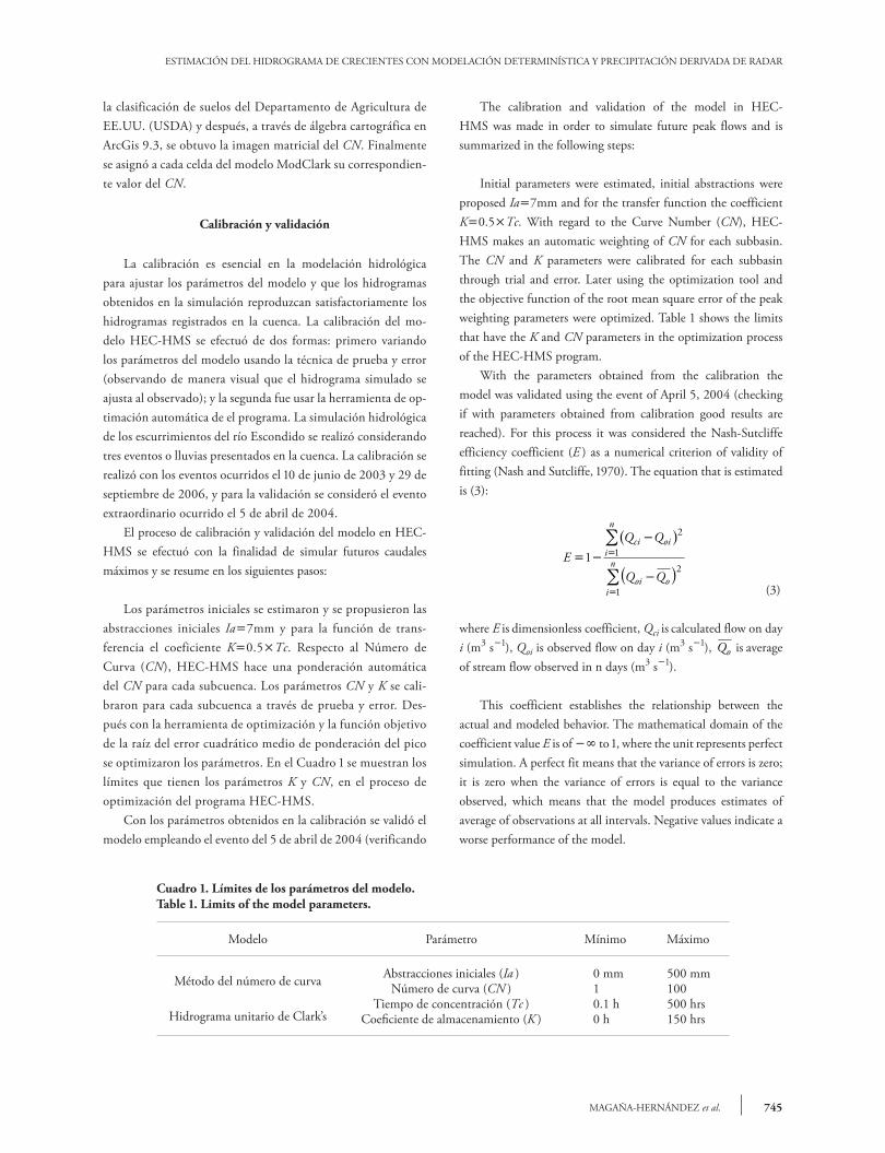
The calibration and validation of the model in HEC-HMS was made in order to simulate future peak flows and is summarized in the following steps:

Initial parameters were estimated, initial abstractions were proposed Ia7mm and for the transfer function the coefficient K0.5Tc. With regard to the Curve Number (CN), HEC-HMS makes an automatic weighting of CN for each subbasin. The CN and K parameters were calibrated for each subbasin through trial and error. Later using the optimization tool and the objective function of the root mean square error of the peak weighting parameters were optimized. Table 1 shows the limits that have the K and CN parameters in the optimization process of the HEC-HMS program. With the parameters obtained from the calibration the model was validated using the event of April 5, 2004 (checking if with parameters obtained from calibration good results are reached). For this process it was considered the Nash-Sutcliffe efficiency coefficient (E ) as a numerical criterion of validity of fitting (Nash and Sutcliffe, 1970). The equation that is estimated is (3):

EQ Q

Q Q

ci oii

n

oi oi

n= −

−( )

−( )=

=

∑

∑1

2

1

2

1 (3)

where E is dimensionless coefficient, Qci is calculated flow on day i (m3 s1), Qoi is observed flow on day i (m3 s1), Qo is average of stream flow observed in n days (m3 s1).

This coefficient establishes the relationship between the actual and modeled behavior. The mathematical domain of the coefficient value E is of to 1, where the unit represents perfect simulation. A perfect fit means that the variance of errors is zero; it is zero when the variance of errors is equal to the variance observed, which means that the model produces estimates of average of observations at all intervals. Negative values indicate a worse performance of the model.

la clasificación de suelos del Departamento de Agricultura de EE.UU. (USDA) y después, a través de álgebra cartográfica en ArcGis 9.3, se obtuvo la imagen matricial del CN. Finalmente se asignó a cada celda del modelo ModClark su correspondien-te valor del CN.

Calibración y validación

La calibración es esencial en la modelación hidrológica para ajustar los parámetros del modelo y que los hidrogramas obtenidos en la simulación reproduzcan satisfactoriamente los hidrogramas registrados en la cuenca. La calibración del mo-delo HEC-HMS se efectuó de dos formas: primero variando los parámetros del modelo usando la técnica de prueba y error (observando de manera visual que el hidrograma simulado se ajusta al observado); y la segunda fue usar la herramienta de op-timación automática de el programa. La simulación hidrológica de los escurrimientos del río Escondido se realizó considerando tres eventos o lluvias presentados en la cuenca. La calibración se realizó con los eventos ocurridos el 10 de junio de 2003 y 29 de septiembre de 2006, y para la validación se consideró el evento extraordinario ocurrido el 5 de abril de 2004. El proceso de calibración y validación del modelo en HEC-HMS se efectuó con la finalidad de simular futuros caudales máximos y se resume en los siguientes pasos:

Los parámetros iniciales se estimaron y se propusieron las abstracciones iniciales Ia7mm y para la función de trans-ferencia el coeficiente K0.5Tc. Respecto al Número de Curva (CN), HEC-HMS hace una ponderación automática del CN para cada subcuenca. Los parámetros CN y K se cali-braron para cada subcuenca a través de prueba y error. Des-pués con la herramienta de optimización y la función objetivo de la raíz del error cuadrático medio de ponderación del pico se optimizaron los parámetros. En el Cuadro 1 se muestran los límites que tienen los parámetros K y CN, en el proceso de optimización del programa HEC-HMS. Con los parámetros obtenidos en la calibración se validó el modelo empleando el evento del 5 de abril de 2004 (verificando

Cuadro 1. Límites de los parámetros del modelo.Table 1. Limits of the model parameters.

Modelo Parámetro Mínimo Máximo

Método del número de curva Abstracciones iniciales (Ia ) 0 mm 500 mmNúmero de curva (CN ) 1 100

Hidrograma unitario de Clark’sTiempo de concentración (Tc ) 0.1 h 500 hrs

Coeficiente de almacenamiento (K ) 0 h 150 hrs

746



si con los parámetros obtenidos en la calibración se llega a bue-nos resultados). Para este proceso se consideró el coeficiente de Eficiencia de Nash-Sutcliffe (E ) como criterio numérico de validez del ajuste (Nash y Sutcliffe, 1970) y se estima con la ecuación 3:

EQ Q

Q Q

ci oii

n

oi oi

n= −

−( )

−( )=

=

∑

∑1

2

1

2

1 (3)

donde E es coeficiente adimensional, Qci es caudal calculado en el día i (m3 s1), Qoi es caudal observado en el día i (m3 s1), Qo es promedio de los caudales observados en los n días (m3 s1).

Este coeficiente establece la relación entre el comporta-miento real y el modelado. El dominio matemático del valor del coeficiente E es de a 1, donde la unidad representa la simulación perfecta. Un ajuste perfecto, quiere decir que la varianza de los errores es cero; vale cero cuando la varianza de los errores es igual a la varianza observada, lo cual signi-fica que el modelo produce estimaciones del promedio de las observaciones en todos los intervalos. Los valores negativos indican un desempeño peor del modelo.

ResultAdos y dIscusIones

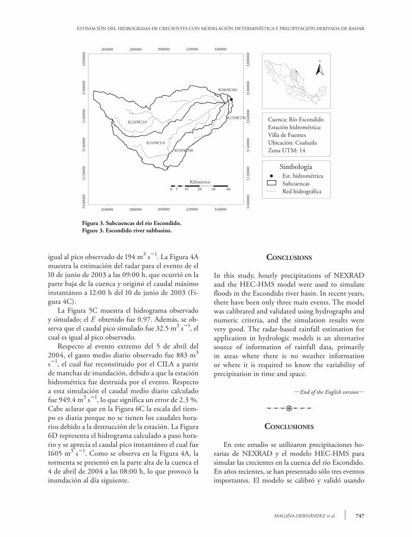
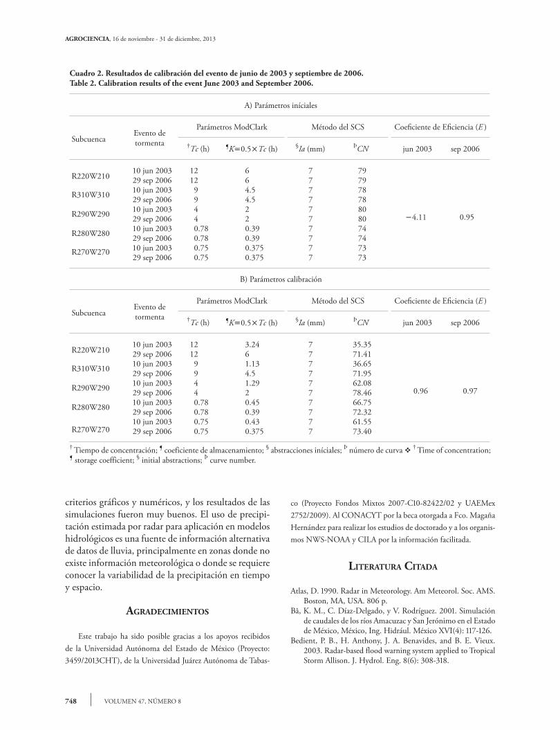
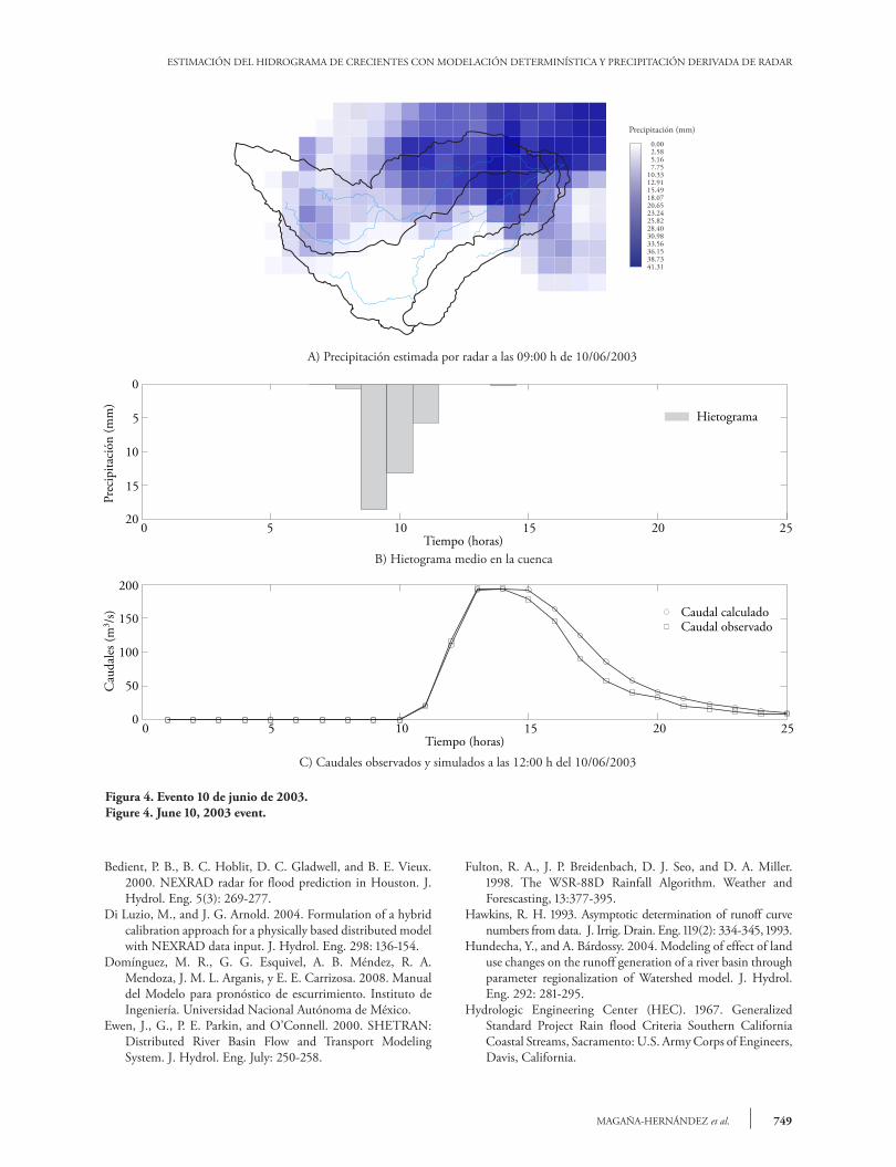
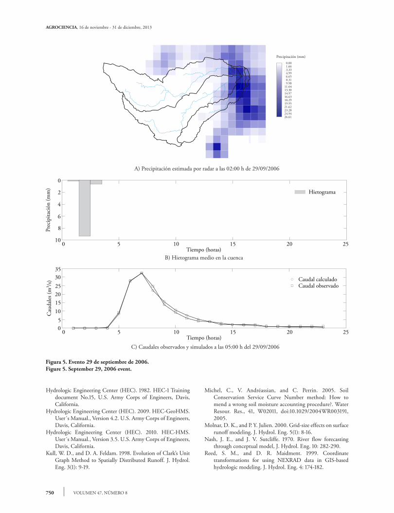
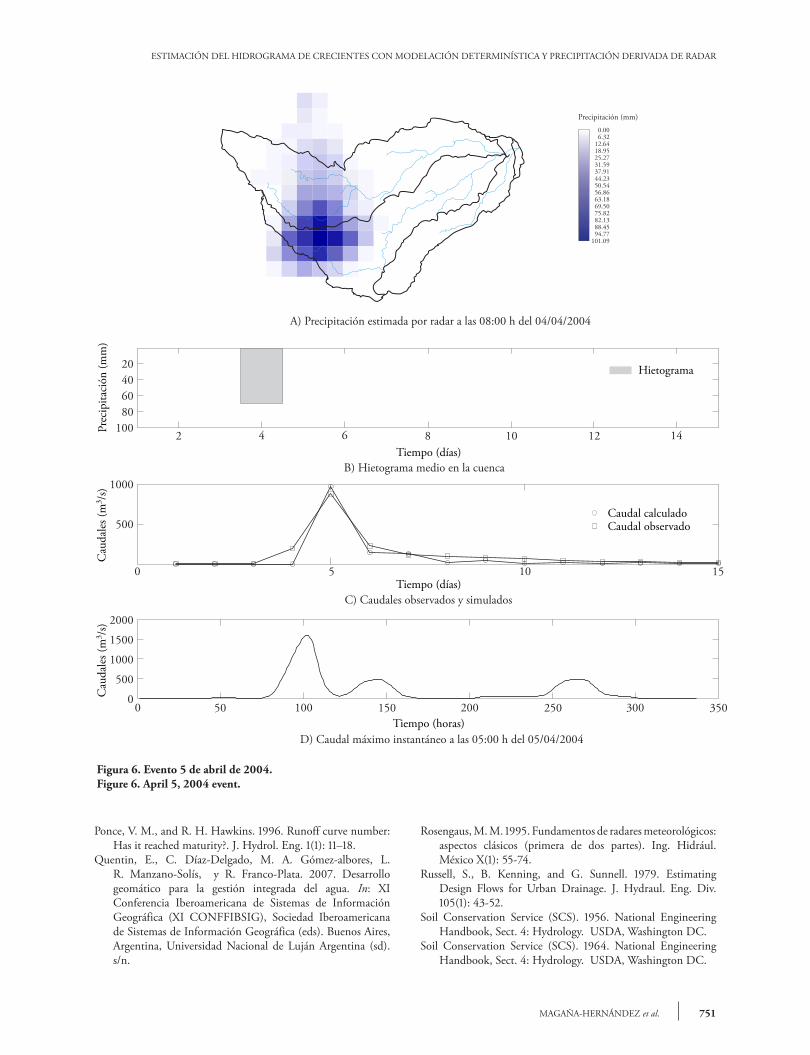
En la Figura 3 se presenta el mapa temático ob-tenido en HEC-GeoHMS de la delimitación de las subcuencas. El caudal máximo ocurrió el 5 de abril de 2004 y en el Cuadro 2 se muestran los resultados obteni-dos en el proceso de calibración. En los dos eventos (10 de junio de 2003 y 29 de septiembre de 2006) se mantuvieron fijos el tiempo de concentración (Tc ) y las abstracciones iniciales (Ia). Para el evento del 10 de junio de 2003, E obtenida con los pará-metros iniciales fue 4.11 (Cuadro 2A). Los valo-res de CN y el coeficiente K se ajustaron para cada subcuenca, los cuales tuvieron mayor efecto en las subcuencas (R22W210 y R310W310) y E fue 0.96 (Cuadro 2B). Respecto a los resultados obtenidos para el evento de septiembre de 2006, E con los parámetros iniciales fue 0.95 (Cuadro 2A), y en la calibración E fue 0.97 (Cuadro 2B). La Figura 4C muestra los hidrogramas observa-do y simulado; el E obtenido fue 0.96. Así mis-mo, el caudal pico simulado fue 194.6 m3 s1 y es

Results And dIscussIon

Figure 3 shows the thematic map obtained in HEC-GeoHMS of the delimitation of the subbasins. The maximum flow appeared on April 5, 2004 and Table 2 shows the results obtained in the calibration process. For both events (June 10, 2003 and September 29, 2006) the time of concentration (Tc ) and initial abstractions (Ia) were kept fixed. For the event of June 10, 2003, the E that was obtained with initial parameters was 4.11 (Table 2A). CN values and K coefficient were adjusted for each subbasin, which had the greatest effect in the subbasins (R22W210 and R310W310), and E was 0.96 (Table 2B). With respect to the results for the September 2006 event, the E with initial parameters was 0.95 (Table 2A), and in the calibration was of 0.97 (Table 2B). Figure 4C shows the observed and simulated hydrographs; the E obtained was 0.96. Likewise, peak flow simulated was 194.6 m3 s1 and is equal to the peak observed of 194 m3 s1. Figure 4A shows the estimates of the radar for the event on June 10, 2003 at 09:00 h, which took place in the lower part of the basin and caused the instantaneous peak flow at 12:00 h on June 10, 2003 (Figure 4C). Figure 5C shows the observed and simulated hydrograph; the E obtained was of 0.97. Also, it is observed that the simulated peak flow was 32.5 m3 s1 which is equal to the peak observed. With respect to the extreme event on April 5, 2004, the average daily spending observed was of 883 m3 s1. This event has been reconstituted by IBWC from stains of flooding, due to the fact that the hydrometric station was destroyed by the event. Regarding this simulation, the average daily flow calculated was 949.4 m3 s1, which means an error of 2.3 %. It should be noted that in Figure 6C the time scale is daily because the hourly flows are not available due to the destruction of the station. Figure 6D represents the hydrograph calculated at hourly step and it shows the instantaneous peak flow, which was 1605 m3 s1. As shown in Figure 6A, the storm took place at the top of the basin on April 4, 2004 at 8:00 h, which caused the flooding the next day.



Figura 3. Subcuencas del río Escondido.Figure 3. Escondido river subbasins.

igual al pico observado de 194 m3 s1. La Figura 4A muestra la estimación del radar para el evento de el 10 de junio de 2003 a las 09:00 h, que ocurrió en la parte baja de la cuenca y originó el caudal máximo instantáneo a 12:00 h del 10 de junio de 2003 (Fi-gura 4C). La Figura 5C muestra el hidrograma observado y simulado; el E obtenido fue 0.97. Además, se ob-serva que el caudal pico simulado fue 32.5 m3 s1, el cual es igual al pico observado. Respecto al evento extremo del 5 de abril del 2004, el gasto medio diario observado fue 883 m3 s1, el cual fue reconstituido por el CILA a partir de manchas de inundación, debido a que la estación hidrométrica fue destruida por el evento. Respecto a esta simulación el caudal medio diario calculado fue 949.4 m3 s1, lo que significa un error de 2.3 %. Cabe aclarar que en la Figura 6C la escala del tiem-po es diaria porque no se tienen los caudales hora-rios debido a la destrucción de la estación. La Figura 6D representa el hidrograma calculado a paso hora-rio y se aprecia el caudal pico instantáneo el cual fue 1605 m3 s1. Como se observa en la Figura 4A, la tormenta se presentó en la parte alta de la cuenca el 4 de abril de 2004 a las 08:00 h, lo que provocó la inundación al día siguiente.

conclusIons

In this study, hourly precipitations of NEXRAD and the HEC-HMS model were used to simulate floods in the Escondido river basin. In recent years, there have been only three main events. The model was calibrated and validated using hydrographs and numeric criteria, and the simulation results were very good. The radar-based rainfall estimation for application in hydrologic models is an alternative source of information of rainfall data, primarily in areas where there is no weather information or where it is required to know the variability of precipitation in time and space.

—End of the English version—

pppvPPP

conclusIones

En este estudio se utilizaron precipitaciones ho-rarias de NEXRAD y el modelo HEC-HMS para simular las crecientes en la cuenca del río Escondido. En años recientes, se han presentado sólo tres eventos importantes. El modelo se calibró y validó usando

748



Cuadro 2. Resultados de calibración del evento de junio de 2003 y septiembre de 2006.Table 2. Calibration results of the event June 2003 and September 2006.

A) Parámetros iníciales

Subcuenca

Evento de tormenta

Parámetros ModClark Método del SCS Coeficiente de Eficiencia (E )

†Tc (h) ¶K0.5Tc (h) §Ia (mm) ÞCN jun 2003 sep 2006

R220W21010 jun 2003 12 6 7 79

4.11 0.95

29 sep 2006 12 6 7 79

R310W310 10 jun 2003 9 4.5 7 7829 sep 2006 9 4.5 7 78

R290W290 10 jun 2003 4 2 7 8029 sep 2006 4 2 7 80

R280W280 10 jun 2003 0.78 0.39 7 7429 sep 2006 0.78 0.39 7 74

R270W270 10 jun 2003 0.75 0.375 7 7329 sep 2006 0.75 0.375 7 73

B) Parámetros calibración

Subcuenca

Evento de tormenta

Parámetros ModClark Método del SCS Coeficiente de Eficiencia (E )

†Tc (h) ¶K0.5Tc (h) §Ia (mm) ÞCN jun 2003 sep 2006

R220W21010 jun 2003 12 3.24 7 35.35

0.96 0.97

29 sep 2006 12 6 7 71.41

R310W310 10 jun 2003 9 1.13 7 36.6529 sep 2006 9 4.5 7 71.95

R290W290 10 jun 2003 4 1.29 7 62.0829 sep 2006 4 2 7 78.46

R280W280 10 jun 2003 0.78 0.45 7 66.7529 sep 2006 0.78 0.39 7 72.32

R270W27010 jun 2003 0.75 0.43 7 61.5529 sep 2006 0.75 0.375 7 73.40

† Tiempo de concentración; ¶ coeficiente de almacenamiento; § abstracciones iníciales; Þ número de curva v † Time of concentration; ¶ storage coefficient; § initial abstractions; Þ curve number.

criterios gráficos y numéricos, y los resultados de las simulaciones fueron muy buenos. El uso de precipi-tación estimada por radar para aplicación en modelos hidrológicos es una fuente de información alternativa de datos de lluvia, principalmente en zonas donde no existe información meteorológica o donde se requiere conocer la variabilidad de la precipitación en tiempo y espacio.

AgRAdecImIentos

Este trabajo ha sido posible gracias a los apoyos recibidos de la Universidad Autónoma del Estado de México (Proyecto: 3459/2013CHT), de la Universidad Juárez Autónoma de Tabas-

co (Proyecto Fondos Mixtos 2007-C10-82422/02 y UAEMex 2752/2009). Al CONACYT por la beca otorgada a Fco. Magaña Hernández para realizar los estudios de doctorado y a los organis-mos NWS-NOAA y CILA por la información facilitada.

lIteRAtuRA cItAdA

Atlas, D. 1990. Radar in Meteorology. Am Meteorol. Soc. AMS. Boston, MA, USA. 806 p.

Bâ, K. M., C. Díaz-Delgado, y V. Rodríguez. 2001. Simulación de caudales de los ríos Amacuzac y San Jerónimo en el Estado de México, México, Ing. Hidrául. México XVI(4): 117-126.

Bedient, P. B., H. Anthony, J. A. Benavides, and B. E. Vieux. 2003. Radar-based flood warning system applied to Tropical Storm Allison. J. Hydrol. Eng. 8(6): 308-318.



Figura 4. Evento 10 de junio de 2003.Figure 4. June 10, 2003 event.

Bedient, P. B., B. C. Hoblit, D. C. Gladwell, and B. E. Vieux. 2000. NEXRAD radar for flood prediction in Houston. J. Hydrol. Eng. 5(3): 269-277.

Di Luzio, M., and J. G. Arnold. 2004. Formulation of a hybrid calibration approach for a physically based distributed model with NEXRAD data input. J. Hydrol. Eng. 298: 136-154.

Domínguez, M. R., G. G. Esquivel, A. B. Méndez, R. A. Mendoza, J. M. L. Arganis, y E. E. Carrizosa. 2008. Manual del Modelo para pronóstico de escurrimiento. Instituto de Ingeniería. Universidad Nacional Autónoma de México.

Ewen, J., G., P. E. Parkin, and O’Connell. 2000. SHETRAN: Distributed River Basin Flow and Transport Modeling System. J. Hydrol. Eng. July: 250-258.

Fulton, R. A., J. P. Breidenbach, D. J. Seo, and D. A. Miller. 1998. The WSR-88D Rainfall Algorithm. Weather and Forescasting, 13:377-395.

Hawkins, R. H. 1993. Asymptotic determination of runoff curve numbers from data. J. Irrig. Drain. Eng. 119(2): 334-345, 1993.

Hundecha, Y., and A. Bárdossy. 2004. Modeling of effect of land use changes on the runoff generation of a river basin through parameter regionalization of Watershed model. J. Hydrol. Eng. 292: 281-295.

Hydrologic Engineering Center (HEC). 1967. Generalized Standard Project Rain flood Criteria Southern California Coastal Streams, Sacramento: U.S. Army Corps of Engineers, Davis, California.

750



Figura 5. Evento 29 de septiembre de 2006.Figure 5. September 29, 2006 event.

Hydrologic Engineering Center (HEC). 1982. HEC-1 Training document No.15, U.S. Army Corps of Engineers, Davis, California.

Hydrologic Engineering Center (HEC). 2009. HEC-GeoHMS. User´s Manual., Version 4.2. U.S. Army Corps of Engineers, Davis, California.

Hydrologic Engineering Center (HEC). 2010. HEC-HMS. User´s Manual., Version 3.5. U.S. Army Corps of Engineers, Davis, California.

Kull, W. D., and D. A. Feldam. 1998. Evolution of Clark’s Unit Graph Method to Spatially Distributed Runoff. J. Hydrol. Eng. 3(1): 9-19.

Michel, C., V. Andréassian, and C. Perrin. 2005. Soil Conservation Service Curve Number method: How to mend a wrong soil moisture accounting procedure?. Water Resour. Res., 41, W02011, doi:10.1029/2004WR003191, 2005.

Molnar, D. K., and P. Y. Julien. 2000. Grid-size effects on surface runoff modeling. J. Hydrol. Eng. 5(1): 8-16.

Nash, J. E., and J. V. Sutcliffe. 1970. River flow forecasting through conceptual model, J. Hydrol. Eng. 10: 282-290.

Reed, S. M., and D. R. Maidment. 1999. Coordinate transformations for using NEXRAD data in GIS-based hydrologic modeling. J. Hydrol. Eng. 4: 174-182.



Figura 6. Evento 5 de abril de 2004.Figure 6. April 5, 2004 event.

Ponce, V. M., and R. H. Hawkins. 1996. Runoff curve number: Has it reached maturity?. J. Hydrol. Eng. 1(1): 11–18.

Quentin, E., C. Díaz-Delgado, M. A. Gómez-albores, L. R. Manzano-Solís, y R. Franco-Plata. 2007. Desarrollo geomático para la gestión integrada del agua. In: XI Conferencia Iberoamericana de Sistemas de Información Geográfica (XI CONFFIBSIG), Sociedad Iberoamericana de Sistemas de Información Geográfica (eds). Buenos Aires, Argentina, Universidad Nacional de Luján Argentina (sd). s/n.

Rosengaus, M. M. 1995. Fundamentos de radares meteorológicos: aspectos clásicos (primera de dos partes). Ing. Hidrául. México X(1): 55-74.

Russell, S., B. Kenning, and G. Sunnell. 1979. Estimating Design Flows for Urban Drainage. J. Hydraul. Eng. Div. 105(1): 43-52.

Soil Conservation Service (SCS). 1956. National Engineering Handbook, Sect. 4: Hydrology. USDA, Washington DC.


752





Whiteaker, T. L., O. Robayo, D. R. Maidment, and D. Obenour. 2006. From a NEXRAD rainfall map to a flood inundation map. J. Hydrol. Eng. 11(1): 37-45.

Whiton, R. C., P. L. Smith, S. G. Bigler, K. E. Will, and A. C. Harbuck. 1998. Hystory of operational use of weather radar by U.S. Weather Services. Part I: The Pre-NEXRAD Era. Am Meteorol. Soc. 13: 219-243.

Xie, H., X. Zhou, R. E. Vivoni, M. H. Hendrick,and E. E. Small. 2005. GIS-based NEXRAD Stage III precipitation database: automated approaches for data processing and visualization. Comput. Geosci. 31: 65-76.

estimaciÓn del hidrograma de crecientes …de eficiencia de nash-sutcliffe que varió de 0.72 a...

Documents