escuela tÉcnica superior de ingenieros de...

ESCUELA TÉCNICA SUPERIOR DE INGENIEROS DE MINAS Y ENERGÍA

Titulación: MÁSTER UNIVERSITARIO EN INGENIERÍA DE MINAS

TRABAJO FIN DE MÁSTER

DEPARTAMENTO DE INGENIERÍA GEOLÓGICA Y MINERA

MEDIDA DE LA FRAGMENTACIÓN DEL ESCOMBRO DE VOLADURA

CON SISTEMAS DIGITALES DE IMÁGENES ‒ SPLIT ONLINE Y SPLIT

DESKTOP ‒ EN LAS MINAS EL ALJIBE (TOLEDO) Y COBRE LAS CRUCES

(SEVILLA).

ANDREA MARTÍNEZ RODRÍGUEZ JULIO DE 2016






(SEVILLA).

REALIZADO POR: ANDREA MARTÍNEZ RODRÍGUEZ

DIRIGIDO POR: PABLO SEGARRA CATASUS

DEPARTAMENTO DE INGENIERÍA GEOLÓGICA Y MINERA

Firma del Prof. Tutor: ………………………………………..

Fecha:





DESKTOP ‒ EN LAS MINAS EL ALJIBE (TOLEDO) Y COBRE LAS

CRUCES (SEVILLA).

Realizado por

Andrea Martínez Rodríguez

Dirigido por

Pablo Segarra Catasus

Departamento de Ingeniería Geológica y Minera

AGRADECIMIENTOS

Me gustaría mostrar mi más sincero agradecimiento al grupo de investigación de

explosivos, especialmente a mi tutor Pablo Segarra de él que tanto he aprendido

por darme la oportunidad de realizar este proyecto, su sabia dirección e

inestimable entrega, así como a Lina Mª López, José Ángel Sanchidrián y Ricardo

Castedo que han constituido una referencia en el campo académico y personal

haciéndome sentir dentro de una familia en la escuela.

Al departamento de Ingeniería Geológica y Minera y todos los docentes de la

escuela que han contribuido a mi formación.

A mi madre por su apoyo incondicional, enseñanzas y cariño que han sido mi

principal guía todos estos años.

A mi pareja y amigos por darme ánimo y alegría cada día.

A mí misma por todo el trabajo y esfuerzo dedicado, de lo que me siento muy

orgullosa.

A todos los que me habéis apoyado, gracias.

I

INDEX

ABSTRACT.................................................................................................................................................... VI

RESUMEN ..................................................................................................................................................... VI

DOCUMENTO 1: MEMORIA.................................................................................................................... 1

1 OBJECTIVE AND SCOPE ................................................................................................................. 2

2 IMPORTANCE OF ROCK FRAGMENTATION CONTROL IN MINING

OPERATIONS ................................................................................................................................................ 3

3 ROCK FRAGMENTATION MEASURING METHODS .......................................................... 5

3.1 SPLIT ONLINE (SOL) AND SPLIT DESKTOP (SD) SYSTEMS ............................................................................. 5

4 CASE STUDY COBRE LAS CRUCES MINE ................................................................................ 9

4.1 DESCRIPTION OF THE MINE SITE ............................................................................................................ 9

4.1.1 Geology .............................................................................................................................. 10

4.1.2 The mine ............................................................................................................................. 11

4.1.3 The processing plant ........................................................................................................... 12

4.2 INSTALLATION OF THE FRAGMENTATION MEASUREMENT SYSTEM ................................................................. 13

4.3 QUALITY ANALYSIS OF THE RESULTING FRAGMENTATION ............................................................................ 17

4.3.1 Relevance of the problem .................................................................................................... 18

4.3.2 Images types analysis ......................................................................................................... 19

4.3.3 Distribution of the characteristic fragmentation parameters ............................................... 20

4.3.4 Offline criteria to filter false positives .................................................................................. 22

4.3.5 Results of the offline criteria ................................................................................................ 24

4.3.6 Offline criteria application ................................................................................................... 25

4.4 FRAGMENTATION ANALYSIS ............................................................................................................... 26

5 CASE STUDY EL ALJIBE QUARRY ........................................................................................... 37

5.1 THE SITE AND FRAGMENTATION MEASUREMENT SYSTEM ........................................................................... 37

5.2 IMAGES IDENTIFICATION.................................................................................................................... 40

5.3 THE BLASTS.................................................................................................................................... 40

5.4 FRAGMENTATION MEASUREMENTS ...................................................................................................... 42

5.4.1 Reliability respect to fines cut-off ........................................................................................ 45

5.4.2 Semi-automatic analysis of fragmentation .......................................................................... 46

5.5 CORRECTION PROCEDURE OF FRAGMENT SIZE DISTRIBUTION CURVES ............................................................ 51

II

5.5.1 Effect of blasting in fragmentation ...................................................................................... 55

6 CONCLUSIONS ................................................................................................................................. 60

7 REFERENCES ................................................................................................................................... 62

7.1 FURTHER READING .......................................................................................................................... 64

DOCUMENTO 2: ESTUDIO ECONÓMICO ...................................................................................... 66

1 PROJECT COSTS .............................................................................................................................. 67

1.1 IMAGE ANALYSIS OF FRAGMENTATION SIZE SOFTWARE .............................................................................. 67

1.2 LABOR COSTS ................................................................................................................................. 67

1.3 TOTAL BUDGET OF THE PROJECT .......................................................................................................... 68

DOCUMENTO 3: ANEXOS ..................................................................................................................... 69

ANNEX A ...................................................................................................................................................... 70

ANNEX B ...................................................................................................................................................... 80

ANNEX C....................................................................................................................................................... 84

III

INDEX OF FIGUES

FIGURE 1: DELINEATED IMAGE........................................................................................................................ 6

FIGURE 2: COBRE LAS CRUCES MINE LOCATION, MAP AND ORTHOPHOTO. .................................................................. 9

FIGURE 3: REPRESENTATIVE CROSS-SECTION OF THE “LAS CRUCES” ORE BODY. 1) DETRITIC AND MAGMATIC ROCKS OF THE

PALEOZOIC SUBSTRATE; 2) MASSIVE SULFIDE BODY; 3) OXIDIZED ORE (GOSSAN); 4) BASAL HORIZON OF THE NEOGENE-

QUATERNARY COVER, INCLUDING GOSSAN BEARING CONGLOMERATES AND GLAUCONITE SANDS; 5) ARCILLAS DE

GIBRALEÓN FORMATION CONSTITUTED BY BLUE MARLS. ............................................................................ 10

FIGURE 4: SPLIT ONLINE FLOW SHEET. ............................................................................................................ 13

FIGURE 5: FRAGMENTATION MEASUREMENT FACILITY ........................................................................................ 14

FIGURE 6: CAMERA POSITION OVER THE TRUCK AND SIGNALING OF THE TRACK. ......................................................... 14

FIGURE 7: TRIGGER R-GAGE SENSOR. ............................................................................................................ 15

FIGURE 8: SPLIT ONLINE INTERFACE. .............................................................................................................. 16

FIGURE 9: CONNECTION SYSTEM IN MINE COBRE LAS CRUCES. ............................................................................ 17

FIGURE 10: BOX PLOT OF LOGARITHMIC SLOPES FOR THE INTERVALS 25-50 MM AND 50-80 MM FOR THE GROUPS OF PASSED

IMAGES OF GOOD QUALITY (25-50G AND 50-80G) AND BAD QUALITY (25-50B AND 50-80B). ......................... 21

FIGURE 11: BOX PLOT OF THE SIZES AT CUMULATIVE PASSING OF 30, 40, …100 FOR GROUPS OF IMAGES CLASSIFIED AS

PASSED GOOD QUALITY AND PASSED BAD QUALITY (IDENTIFIED WITH THE LETTERS G AND B RESPECTIVELY). ............ 21

FIGURE 12: BOX PLOT OF THE PRODUCT OF THE ABSOLUTE VALUE OF THE LOGARITHMS OF THE OF Z-SCORE VALUE, PLZ, OF THE

SLOPES 25-50 AND 50-80 AND SIZES X50, X60, X70 AND X80 FOR ALL PASSED IMAGES, FALSE POSITIVES AND PASSED

GOOD QUALITY. ............................................................................................................................... 22

FIGURE 13: BOX PLOT OF THE PRODUCT OF THE ABSOLUTE VALUE OF THE Z-SCORE LOGARITHM, PLZ, OF THE X50, X60, X70 AND

X80 OF ALL PASSED IMAGES, INCLUDING GOOD AND BAD QUALITY, AND GOOD PASSED AND BAD. THE GREEN RECTANGLE

INDICATES THE DELETED PHOTOS USING THE PERCENTILE 75 % (P75) OF ALL PASSED IMAGES. ............................. 23

FIGURE 14: MEAN SIZE DISTRIBUTION CURVES FOR 11TH

, 15TH

, 16TH

AND 17TH

SEPTEMBER, 2014. RED LINE: ALL PASSED

PHOTOS. BLACK LINE: PASSED GOOD QUALITY IMAGES. BLUE: REMAINING CURVES AFTER FILTERING. ..................... 24

FIGURE 15: BOXPLOT OF THE X80 FOR EACH BLAST. ............................................................................................ 27

FIGURE 16: MEDIAN SIZE X50 VERSUS X80 FOR THE BLAST MONITORED IN COBRE LAS CRUCES. ...................................... 28

FIGURE 17: RELATIONSHIP BETWEEN X80 AND THE SPECIFIC EXPLOSIVE CONSUMPTION. ............................................... 33

FIGURE 18: SPECIFIC CONSUMPTION VERSUS ITS CORRESPONDING BENCH. .............................................................. 34

FIGURE 19: RESULTING X80 OF THE BLAST PERFORMED IN EACH BENCH. ................................................................... 34

FIGURE 20: X80 VERSUS POWDER FACTOR FOR EACH BENCH LEVEL. ....................................................................... 35

FIGURE 21: EL ALJIBE QUARRY LOCATION, MAP AND ORTHOPHOTO. ...................................................................... 37

FIGURE 22: PRIMARY PHASE OF THE CRUSHING PLANT OUTLINE. ........................................................................... 38

FIGURE 23: SCALING PROCEDURE FOR THE IMAGES TAKEN IN EL ALJIBE. .................................................................. 39

FIGURE 24: QUARRY CONDITIONS IN BLAST B6. ................................................................................................. 40

FIGURE 25: CHEVRON BLAST PATTERN. ........................................................................................................... 41

IV

FIGURE 26: SIZE DISTRIBUTION CURVES FROM BLAST B1. ..................................................................................... 43

FIGURE 27: SIZE DISTRIBUTION CURVE FROM AN IMAGE FROM BLAST B6. ................................................................ 44

FIGURE 28: SIZE DISTRIBUTION CURVES OF IMAGES WITH A FEW LARGE FRAGMENTS (A) OR WITH A WRONG DELINEATION (B).

................................................................................................................................................... 45

FIGURE 29: PHOTOGRAPH AND DELINEATION OF CURVE 28A. .............................................................................. 45

FIGURE 30: PHOTOGRAPH AND DELINEATION OF CURVE 28B................................................................................ 45

FIGURE 31: BOXPLOT OF THE WHOLE SET OF IMAGES PER EACH BLAST (NOTE THAT THE SCALES OF THE ORDINATES AXIS ARE

DIFFERENT IN EACH GRAPH). ............................................................................................................... 46

FIGURE 32: FRAGMENTATION FROM SPLIT ONLINE (AUTOMATIC MODE) AND SPLIT DESKTOP (SEMI-AUTOMATIC MODE) OF

THE SETS OF 20 IMAGES RANDOMLY SELECTED FOR EACH BLAST (BLUE LINES: SPLIT ONLINE, CYAN LINES: SPLIT

DESKTOP, BLACK LINE: SPLIT ONLINE MEDIAN, RED LINE: SPLIT DESKTOP MEDIAN)............................................ 49

FIGURE 33: PLOT OF DIFFERENT SIZES FROM SPLIT ONLINE AND SPLIT DESKTOP. ....................................................... 50

FIGURE 34: THE MEDIAN SIZE DISTRIBUTION CURVES OF SPLIT ONLINE (SOL) A ND SPLIT DESKTOP (SD) AND ITS CORRECTION

BY SCALE BELT VALUES (SOLC AND SDC). ................................................................................................ 53

FIGURE 35: PLOT OF DIFFERENT SIZES FROM SPLIT ONLINE CORRECTED AND SPLIT DESKTOP CORRECTED. ..................... 54

FIGURE 36: LINEAR REGRESSION APPLIED TO X20, X50, AND X80 CORRECTED VERSUS POWDER FACTOR (BLUE LINE) AND SAME

LINEAR REGRESSION EXCLUDING BLAST B6 (RED LINE). ................................................................................ 56

FIGURE 37: LINEAR REGRESSION APPLIED TO X20, X50, AND X80 CORRECTED VERSUS THE SPECIFIC USEFUL WORK. ............... 58

FIGURE 38: LINEAR REGRESSION APPLIED TO X20, X50, AND X80 CORRECTED VERSUS SPECIFIC HEAT OF EXPLOSION. ............. 59

V

INDEX OF TABLES

TABLE 1: QUALITY OF THE AUTOMATIC CLASSIFICATION....................................................................................... 18

TABLE 2: QUALITY OF PASSED IMAGES TO THE DATES 11TH

, 15TH

, 16TH

AND 17TH

OF SEPTEMBER ................................... 20

TABLE 3: PASSED IMAGES OBTAINED AT 11TH,15TH,16TH AND 17TH

OF SEPTEMBER, 2014. RESULTS OF FILTERING: PERCENTILE

75 % OF THE ABSOLUTE PRODUCT OF THE Z-SCORE OF THE LOGARITHM OF SIZES X50, X60, X70 AND X80. ................. 23

TABLE 4: SUMMARY OF THE PARAMETERS OF THE CURVES FILTERED MONTHLY. ......................................................... 25

TABLE 5: RECORDED IMAGES BY BLAST. .......................................................................................................... 26

TABLE 6: P-VALUE OF X80 FOR THE WILCOXON RANK SUM TEST (THE TABLE HAS BEEN SPLIT IN THREE PAGES TO FACILITATE ITS

READING). ...................................................................................................................................... 29

TABLE 7: DISPARITY OF X80 BETWEEN BLASTS. ................................................................................................. 32

TABLE 8: BLAST PARAMETERS SUMMARY. ........................................................................................................ 41

TABLE 9: SPECIFIC CHARGE. ......................................................................................................................... 42

TABLE 10: P-VALUE OF WILCOXON RANK SUM TEST ........................................................................................... 47

TABLE 11: P-VALUE OF WILCOXON RANK SUM TEST FOR SPLIT ONLINE AND SPLIT DESKTOP CURVES. ............................. 48

TABLE 12: FIT PARAMETERS FOR SPLIT ONLINE VERSUS SPLIT DESKTOP. .................................................................. 50

TABLE 13: FIT PARAMETERS FOR SPLIT ONLINE CORRECTED VERSUS SPLIT DESKTOP CORRECTED. ............................... 54

TABLE 14: REGRESS PARAMETERS FOLLOWING LOG(XK)=A·LOG(X)B FOR POWDER FACTOR ABOVE GRADE. ....................... 55

TABLE 15: REGRESS PARAMETERS FOLLOWING LOG(XK)=A·LOG(X)B EXCLUDING

B6...................................................... 56

TABLE 16: USEFUL WORK AND HEAT OF EXPLOSION ENERGY. ................................................................................ 57

TABLE 17: REGRESS PARAMETERS FOR SPECIFIC USEFUL WORK ENERGY EWU. ............................................................ 57

TABLE 18: REGRESS PARAMETERS FOR SPECIFIC HEAT OF EXPLOSION ENERGY EQ. ....................................................... 57

TABLE 19: INSTALLATION AND SOFTWARE EXPENSES. ......................................................................................... 67

TABLE 20: PERSONNEL COSTS. ..................................................................................................................... 68

TABLE 21: TOTAL COSTS. ............................................................................................................................ 68

TABLE 22: BUDGET. .................................................................................................................................. 68

VI

ABSTRACT

Split Online, a continuous fragmentation monitoring system by automatic image

analysis, has been installed in the open pit mine Cobre las Cruces (Sevilla, Spain)

and in the quarry El Aljibe (Toledo, Spain) to analyze blasted rock from 51 and 6

blasts, respectively. The resulting fragmentation is significantly finer in Cobre las

Cruces. In this site the system is not able to discard bad quality photographs, and

an offline criterion to filter these images has been developed. The analysis of

blasting and fragmentation data prevents to detect the effect of the powder factor

on the resulting fragmentation. Very fine sizes may be the reason behind this

result.

In El Aljibe quarry fragmentation results were calibrated by belt scale

measurements at 25 and 125 mm. Twenty images were randomly selected in each

blast to correct manually the automatic delineation (i.e. semi-automatic analysis)

made by Split Desktop. The automatic analysis leads to a coarser fragmentation

and statistically different than the semi-automatic analysis. Only the data from the

semi-automatic analysis (i.e. manual correction) after calibration allows detecting

the influence of the blast in the fragmentation, and relations between x80 and x50

and the specific energy have been derived.

RESUMEN

Split Online, un sistema de monitoreo de fragmentación mediante análisis

automático de imagen, ha sido instalado en la mina de Cobre las Cruces (Sevilla,

España) y la cantera El Aljibe (Toledo, España) para analizar escombro de voladura

de 51 y 6 voladuras respectivamente. La fragmentación resultante es

significativamente más fina en Cobre las Cruces. En esta mina el sistema no es

capaz de descartar imágenes de mala calidad por lo que un criterio offline para

filtrar dichas imágenes ha sido desarrollado. El análisis de la voladura y los datos

de fragmentación no permiten detectar el efecto del consumo específico de

explosivo en la fragmentación resultante. Tamaños muy finos pueden ser la razón

detrás de ese resultado.

VII

En el Aljibe los resultados de la fragmentación fueron calibrados mediante las

medidas recogidas por básculas para los tamaños 25 y 125 mm. La delineación

automática de veinte imágenes seleccionadas aleatoriamente en cada voladura fue

corregida manualmente (es decir, análisis semi-automático) mediante Split

Desktop. El análisis automático conduce a una fragmentación más gruesa y

estadísticamente diferente al análisis semi-automático. Solo los resultados del

análisis semi-automático (es decir, corrección manual) después de la calibración

permiten detectar la influencia de la voladura en la fragmentación, y las relaciones

entre x80 y x50 y la energía específica.




(SEVILLA).

DOCUMENTO 1: MEMORIA

2

1 Objective and scope

Rock fragmentation control is a fundamental action in mining due to its

consequences on the whole process: loading, hauling, crushing, classification and

processing. The overall performance depends on the particle size distribution of

the material obtained at the first stage of the mining and treatment process (i.e.

drilling and blasting stages). Generally an assessment of rock fragmentation by

blasting involves an unaffordable interruption of the run of mine (Ouchterlony,

2003). For that reason, the use of digital image analysis is a well-accepted method

to measure the resulting fragmentation. This technique developed through the

1990s has the advantage of allowing the normal progress of mining operations

including a continuous measurement. Digital image analysis techniques present,

however, inherent limitations that generate errors which have to be taken into

consideration to its practical application (Sanchidrián et al., 2005, 2008).

In this Master Thesis, the performance of a digital system of images working fully

automatic and semi-automatic will be discussed. For this purpose, the continuous

fragmentation monitoring system Split Online (Split Engineering, 2001) has been

installed first in the quarry El Aljibe (Toledo, Spain) and in the open pit mine Cobre

las Cruces (Sevilla, Spain). This system delineates automatically the edge of the

grains which appear in a photograph with a size greater than the resolution of the

system. The system obtains the volume of the delineated particles from the

measured areas. Generally this delineation can be modified afterwards by an

operator.

In El Aljibe, the system recorded images of fragmented rock from six blasts which

are processed automatically with Split Online (fully automated delineation) and

with Split Desktop (semi-automated delineation). The results obtained by both

methods are compared and analyzed statistically.

In Cobre las Cruces Split Online was used to monitor fragmentation of the ore

during ten months. An offline filter was developed, designed and validated to

3

eliminate the bad quality images, which can generate a bias in the measurement. In

both sites the effect of blasting in fragmentation was assessed.

2 Importance of rock fragmentation control in mining

operations

Concerning costs in mining, fragmentation is a determining aspect. In the quarries

and mines where processing consists on comminution and classification processes,

such as aggregates industry, the price of the final product directly depends on the

fragmentation size due to the fact that some fragment fractions are more valuable

than others. In these cases, the reduction of the amount of fines is totally

preferable. There are cases such as limestone and cement quarries with up to 30 %

of fines which are useless and cannot be sold in the market (Moser, 2003). An

example of the detriment occasioned by the presence of fines is the loss of

mechanical resistance in aggregates. In metallic operations where the processing

involves ore separation and concentration, such as leaching, the permeability will

be reduced and, therefore, the recovery also when 12 % of the material is smaller

than 150 µm (Onederra et al., 2004). In the same way, fines may be a problem in

coal processing. On the other hand, lixiviation process in metallic mining requires

very uniform fragmentation. The average annual consumption of raw materials in

Europe is around 10 tons per person that means about 1 ton/person has to be put

on waste dumps annually (Moser, 2003). So, this is not only an economic problem

but also an environmental issue.

It is then important to know and control the fragmented rock size in each of the

size reduction stages, beginning from the blasted rock (about the 50 % of the raw

materials are mined by this method). As Ouchterlony (2003) highlighted, this may

be achieved with a better-controlled blast technique involving less scatter in the

outcome. Even although this scatter is caused mainly by the geological conditions,

the blasting characteristics have an important role. Previously, the blasting

influence studies were focused mainly on making more efficient the loading

process and avoiding the production of oversize fragments (Ouchterlony, 2003).

4

Nevertheless, downstream effects are taking more relevance nowadays. Energy

prices have been raised last years and grinding consumes by far the higher

amount.

The size distribution of the blasted rock has a direct influence on the plant. In

order to reduce the energy costs it is possible to decrease the feed size of the

primary crusher. This could be achieved through a decrease of the Bond’s work

index and/or increase the amount of undersize that bypasses the crushing stages

(Ouchterlony, 2003). Coarse sizes will decrease the throughput of the primary

crushing generating downtimes because of stuck material. Besides, a poor

fragmentation will require more energy consumption in successive comminution

stages. Blasting produces micro and macro cracks in the fragments which

stimulate the breakage at the different stages of comminution decreasing the

energy consumption and wear and increasing productivity. Nevertheless the

internal fracturing cannot be measured directly as it can be made with the

resulting fragmentation by blasting.

In order to establish a fragmentation control system, both the problem and the

target to be optimized must be analyzed in detail. This may consists of:

- Minimize or maximize a given fragment fraction or size.

- Increasing primary crushing productivity.

- Increasing the global productivity: reducing maintenance costs, spare

pieces consumption, energy expenditures, etc.

Next, the best indicators of the process have to be selected to analyze their

response to the blast and processing variations. These decisions require an

extended knowledge of the operation.

5

3 Rock fragmentation measuring methods

Due to its elevated costs, sieving is not a feasible measuring technique. Fortunately,

there are other methods to evaluate fragmentation such as installing belt scales at

certain points of the plant or using digital image analysis systems. The decision of

the methods to be used varies at each mine.

The main advantage of image analysis systems is that it does not interrupt

production. This technique has been already developed for almost thirty years and

despite its restrictions is considered the only practical tool for evaluating

fragmentation of the run of mine (Sanchidrián et al., 2005). In order to reduce the

inherent errors of the digital analysis, Latham et al. (2003) proposed a calibration

through sieving which can be realized easily in the case of a conveyor belt but

becomes more complicated when fragmentation is assessed in the mine site before

primary crushing. Besides of this, the location of the measurement system depends

on the aim of the fragmentation control. For example, if it is desired to know the

result of a blast design, a measure taken downstream the primary will difficult the

analysis of its effect on fragmentation. In most cases, the boulders that cannot be

loaded by the shovel without performing mechanical breakage are not considered

in fragmentation measurements. Digital imagine analysis systems extrapolate the

third dimension, which causes errors due to the overlapping between fragments

and the shape of the fragments. The fact that photographed rock is not always

representative of all the blasted material may be another source of error.

The most significant programs to obtain granulometric distributions by means of

image analysis are Fragscan (Schleifer & Tessier, 2000), Split (Split Engineering,

2001), PowerSieve® and Wipfrag (Maerz & Palangio, 1999).

3.1 Split Online (SOL) and Split Desktop (SD) systems

In this Master thesis, two different products from Split: Split Online (SOL) and Split

Desktop (SD) have been used. Both are able to delineate automatically the edges of

6

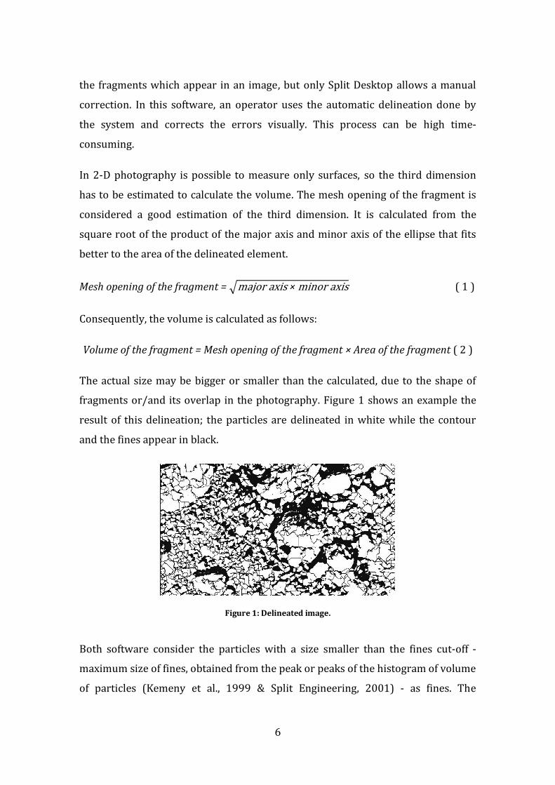
the fragments which appear in an image, but only Split Desktop allows a manual

correction. In this software, an operator uses the automatic delineation done by

the system and corrects the errors visually. This process can be high time-

consuming.

In 2-D photography is possible to measure only surfaces, so the third dimension

has to be estimated to calculate the volume. The mesh opening of the fragment is

considered a good estimation of the third dimension. It is calculated from the

square root of the product of the major axis and minor axis of the ellipse that fits

better to the area of the delineated element.

Mesh opening of the fragment = ( 1 )

Consequently, the volume is calculated as follows:

Volume of the fragment = Mesh opening of the fragment × Area of the fragment ( 2 )

The actual size may be bigger or smaller than the calculated, due to the shape of

fragments or/and its overlap in the photography. Figure 1 shows an example the

result of this delineation; the particles are delineated in white while the contour

and the fines appear in black.

Figure 1: Delineated image.

Both software consider the particles with a size smaller than the fines cut-off -

maximum size of fines, obtained from the peak or peaks of the histogram of volume

of particles (Kemeny et al., 1999 & Split Engineering, 2001) - as fines. The

7

interstices and voids are also taken as fines. There is an increment in the smaller

fractions when the material of an analyzed photography is sieved. Several authors

have concluded that the smaller particles are underestimated in image analysis

(Ouchterlony, 2003). Some reasons are:

- Fines are segregated under the surface.

- Some packs of fines are taken as big blocks.

- Fines sizes are under the image resolution.

The total area of fines is the area of black pixels plus the area of the particles

smaller than the fines cut-off:

Total area of fines = Area of fragments smaller than fines cut-off + FF × black area

( 3 )

Where FF is the fit factor of fines, which varies between 25 % in rocks with few

fines to 150 % or even more in rocks with a lot of fine material. It can be

considered constant for a location and specific rock. Then the percentage of total

volume of material with a size smaller than the fines cut-off is calculated:

% volume = 100 ×

( 4 )

Where the total area is the sum of the area of fines plus the area of the particles

delineated with an area bigger than the fines cut-off. The part of the size

distribution curve which corresponds to sizes bigger than the fines cut-off has to

be corrected and fitted with the point which corresponds to fines cut-off size and

the calculated volume percentage. Thus, the fines factor influences the whole

resultant curve and, for that reason, has to be calibrated.

Finally, the system extrapolates the size distribution curve for sizes smaller than

the fines cut-off using the Schuhmann distribution or Rosin-Rammler distribution

according to the decision of the user:

8

Schuhmann distribution:

m

max

cf

x

xxxP

100)( ( 5 )

Rosin-Rammler distribution:

n

x

x

cfexxP

50

693.0

1100)( ( 6 )

Where P(x) is the cumulative volume passing at sizes x smaller than the fines cut-

off (xcf), xmax is the maximum size, m is a constant, x50 is the median size and n is the

index uniformity. The parameters of each distribution are obtained from the fines

cut-off and a value slightly greater than the fines cut-off.

9

4 Case study Cobre las Cruces mine

The Split Online monitoring system installed in the mine Cobre las Cruces (Sevilla,

Spain) allows estimating automatically the fragmentation size of blasted material

using photographs taken over the trucks that haul the material to the

homogenizing muckpiles. The system and the mine site are described below.

4.1 Description of the mine site

The mine Cobre las Cruces is an open pit located 20 km Northwest of Seville, in the

municipality of Gerena (Figure 2). It is placed in a copper deposit exceptionally

rich, 7 to 12 times higher in copper than other similar ore bodies. The original ore

reserves were 17,6 Mt of grading 6,2 % copper. The project has an operating life of

10 years plus two years for closure, according to the 14,1 Mt of reserves of grading

5,4 % Cu calculated in December 2012. A prolongation of its life time by about 15

years exploiting the Gossan and primary sulfides is being studying.

Figure 2: Cobre las Cruces mine location, map and orthophoto.

Modified from IBERPIX Instituto Geográfico Nacional.

10

4.1.1 Geology

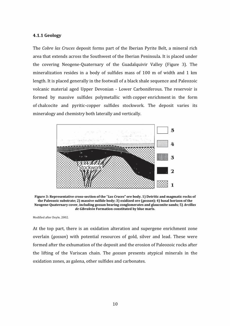
The Cobre las Cruces deposit forms part of the Iberian Pyrite Belt, a mineral rich

area that extends across the Southwest of the Iberian Peninsula. It is placed under

the covering Neogene-Quaternary of the Guadalquivir Valley (Figure 3). The

mineralization resides in a body of sulfides mass of 100 m of width and 1 km

length. It is placed generally in the footwall of a black shale sequence and Paleozoic

volcanic material aged Upper Devonian - Lower Carboniferous. The reservoir is

formed by massive sulfides polymetallic with copper enrichment in the form

of chalcocite and pyritic-copper sulfides stockwork. The deposit varies its

mineralogy and chemistry both laterally and vertically.

Figure 3: Representative cross-section of the “Las Cruces” ore body. 1) Detritic and magmatic rocks of the Paleozoic substrate; 2) massive sulfide body; 3) oxidized ore (gossan); 4) basal horizon of the

Neogene-Quaternary cover, including gossan bearing conglomerates and glauconite sands; 5) Arcillas de Gibraleón Formation constituted by blue marls.

Modified after Doyle, 2002.

At the top part, there is an oxidation alteration and supergene enrichment zone

overlain (gossan) with potential resources of gold, silver and lead. These were

formed after the exhumation of the deposit and the erosion of Paleozoic rocks after

the lifting of the Variscan chain. The gossan presents atypical minerals in the

oxidation zones, as galena, other sulfides and carbonates.

11

4.1.2 The mine

Currently, Cobre las Cruces mine belongs to the Canadian company First Quantum.

The pit has about 900 meters width and 250 meters depth. Its annual processing

capacity is 1,3 Mt. The stripping ratio is 12,7:1 with 10 Mt of removed waste each

year. Annually the ore production is 72 000 t while the production of its lifetime

will be 996 000 t (Espí et al., 2010).

The blasts are designed using JKSimblast (Soft-Blast, 2006) and are located by the

topography department through GPS. Afterwards, this information is provided to

the driller. Always that it is possible, the blast is made only over ore. The nominal

blasting and geological parameters are:

- The subdrill length is 0,5 m to ore and 1 m to gangue.

- The burden and spacing are 4,5 and 5 m respectively, and the boreholes

diameter is 51/2” (140 mm).

- Down hole intiation with 450 g boosters.

- Emunex 8000 (emulsion: ANFO 80:20) as explosive.

- Explosive linear density is 19 kg/m and the powder factor 0,5 kg/m3.

- Between 5 and 8 rows.

- Delay between holes is 9 ms.

The ore is always loaded during the morning shift. Commonly, the material is

loaded by one excavator and occasionally by two. The operator records which

block is loading and for how long.

Hauling is made by 777 CAT or Komatsu 785 trucks of 100 t. The dimensions of all

the trucks are similar, around 5 meters width and 5,2 meters height on the tuck

box. The ore hauled never protrudes the box height due to its high density (4

t/m3). Those trucks which load ore include a weight scale. A blasting needs

approximately 200 trucks to be loaded.

After hauling, the ore is distributed in homogenization piles. Generally there are

eight piles under operation. Different zones are marked to distinguish grades. Iron

12

sulfate needed to the lixiviation is placed on the top of the pile. The pile material is

loaded with a bucket perpendicularly to the direction of dumping and it is

transported to the plant. During this operation the grain size is further reduced

due its weakness.

In the mine there are four kinds of logs:

- Blasting log: It is developed in Access Microsoft software and includes the

coordinates of drill holes position and crest and toe of the bench measured

by GPS, average mass of the drill holes, videos, etc

- Block log: It is developed in Excel Microsoft software and includes

information such as block mass and ore grade from analysis of blasting

chips.

- Load log: It is an Excel Microsoft. It shows the time needed by the excavator

to load each block, the mass measured by the trucks weight scale and the

pile in which the material is hauled.

- Plant log: Electricity consumption, …

At the moment there is not truck dispatch in the mine.

4.1.3 The processing plant

A hydrometallurgical process is used instead of the pyrometallurgical processing,

more contaminating and conventional. The average recovery of the deposit is 97 %

and the metallurgic recovery is 91,4 %. The plant is classified as “Clean

Technology”.

The primary is a jaw crusher with a feed size of 650 mm and an output size of 150

mm. The secondary milling consists of cone mills. Fines do not hinder the

lixiviation, but they disturb the performance of milling. The pulp flows into the

leaching circuit, dissolving the copper in the ore into an aqueous solution. The

aqueous solution with dissolved copper goes to a solvent extraction circuit, where,

by means of a selective agent for copper extraction, purification and concentration

13

is achieved. The aqueous solution flows to the electrowinning cells, where the

copper is deposited on stainless steel cathodes. Copper cathodes, with a very high

purity, (99,999 % pure copper classed as “Grade A”) are sent directly to the

industry.

4.2 Installation of the fragmentation measurement system

The Split Online hardware is constituted by a set of concatenated modules that

process the data, see Figure 4. Its functions are described below.

Figure 4: Split Online flow sheet.

The camera module is activated by a trigger. Then, the delineation module and

calculation module convert the photograph into size distribution measurements

and stores this information in a database in Microsoft Excel. Generally the system

does not save any photos. But in this project it was considered important to store

also the images so an external hard disc was installed in the Split PC for this

purpose. The information about the blasts (timing, amount of explosives used, …)

is also stored for the later analysis.

The camera which takes the material photographs is placed 10,5 meters over the

truck in the way to the homogenizing pile, see Figure 5. A steel cable was used to

avoid the fall of the facility due to the camera weight. A switch was added at the

bottom part to be able to make changes without climbing to the top. It is not

needed an artificial lighting because loading is made during the morning shift, so

there is enough natural light to take the photos of the material.

Trigger Camera module

Delineation module

Calculation module

Database Hard disc

Blasts

Split PC

14

Figure 5: Fragmentation measurement facility

The electrical power source of the camera is supplied by solar panels of 24 V,

autonomous during 48 hours in the dark. The camera has its own IP direction to be

able to display online the fragmentation results in a computer placed at the offices

of the mine, and to send the photographs via a wireless LAN system.

The camera was oriented perpendicularly to the truck box. Otherwise, there would

be a depth effect and thus a deviation in Split Online measurements. The digital

settings of the camera are used to determine the measurement window. Besides

that, the limits of the track where the haul trucks have to be driven were first

marked on the floor (Figure 6).

Figure 6: Camera position over the truck and signaling of the track.

The camera was triggered when an object was detected in its working area using a

R-Gage sensor (Banner Engineering Corp., see Figure 7). One to three photographs

of the load hauled by the trucks were taken. This radar-based system for detection

of moving and stationary targets emits a beam of high-frequency radio waves from

1.5 m 2m 2.5m

5 m

5.5 m

Cámara y focos

ESTEOESTE West East

Camera

Switch

15

an internal antenna to detect objects containing metal, water or similar high-

dielectric materials with a range from 2 to 24 m. In this case it was set to 4 m. The

distance from the sensor to the object is calculated based on the time delay of the

return reflected signal. Its sensing functions can be adjusted to ignore objects

beyond the set point and are unaffected by weather conditions. The camera scale

was 4.0 px/cm. Several tests were made to adjust the trigger so the material in the

box can be photographed when trucks speed was low, around 20 km/h.

Figure 7: Trigger R-Gage sensor.

Once the installation was finished, it was established the available personal to

realize electric maintenance and computing tasks which could be requested.

Afterwards, the settings of the Split Online software were made during the system

commissioning, such as the watchdog, project properties and system project.

Regarding the software, the most important commands of Split are:

- File: Related to the images. It allows to open a imagen, close it, …

- Project: The settings of each project are saved including aspects such as the

delay between photos, etc.

- System: It is possible to change the working mode. In this case is used the

engineering mode which allows to change the system parameters if it is

desired.

- View: A selection of the windows to visualize (Figure 8). The Status Window

shows a yellow light if the system is waiting for new images and green if a

photograph is taken. It is possible to connect/disconnect the connection

16

between the camera module and the delineation module in the Operations

Window by pressing the red point or the arrow respectively. This action can

be also done by means of the Connection Window (right bottom of the

mouse and select the option stop). It is remarkable that stopping the

connection also stops the data log.

Figure 8: Split Online interface.

The output data obtained from 00:00 h to 24:00 every day is saved in a new

Microsoft Excel file in the hard disc so the file will not be able to be opened until

the following day. The data is structured by rows including the exact time and date

when each photograph was processed.

A remote connection to the computer in mine Cobre las Cruces where all the data of

Split Online is stored was allowed to Universidad Politécnica de Madrid. The

connection system inside the mine is shown in the Figure 9:

Operations Window

Status Window

Connection Window

17

Figure 9: Connection system in mine Cobre las Cruces.

The connection in the Split equipment was designed by the IT team of mine Cobre

las Cruces. This connection is made via OpenVPN in safe mode to Windows. The

remote access is made by the free software Team Viewer.

4.3 Quality analysis of the resulting fragmentation

The camera trigger is activated whenever the sensor detects any movement in its

area of influence. For that reason, every time that any kind of vehicle goes through

the track where the system is installed a photograph is taken. Split Online software

has a filter to discard automatically photos that include more elements than only

rock fragments and store it as failed images, while the photos to be analyzed will

be classified like passed. However, frequently this automatic filter includes in the

passed category photos of the floor under the camera or parts of the truck.

These images classified wrongly by Split Online have to be eliminated due to their

effect on the fragmentation measurements. The analysis below shows a large

amount of false positives - images wrongly classified as blasted material by the

18

system. This makes necessary to define an offline criteria which improve the filter

results of Split Online.

4.3.1 Relevance of the problem

With the aim of assessing the quality of the automatic passed/failed classification,

the quality of all the images taken by the camera in September, 2014 has been

manually analyzed. Table 1 is a summary of the main results of this analysis. The

analysis shows that 39 % of the images are false positives. On the other hand, only a

3 % of the images are false negatives – images with blasted material wrongly

considered like failed. These images are classified as failed although its quality was

good.

Table 1: Quality of the automatic classification

Images number Percentage

Date Passed photos1

False positives

Failed photos

False negatives

False positives

False negatives

01/09/2014 0 0 0 0 0 0 02/09/2014 0 0 27 0 0 0 03/09/2014 0 0 9 0 0 0 04/09/2014 4 4 5 0 100 0 05/09/2014 0 0 0 0 0 0 06/09/2014 1 1 17 0 100 0 07/09/2014 0 0 27 0 0 0 08/09/2014 0 0 14 0 0 0 09/09/2014 22 5 148 0 23 0 10/09/2014 78 24 827 70 31 8 11/09/2014 268 104 1506 67 39 4 13/09/2014 32 10 436 30 31 7 14/09/2014 0 0 9 0 0 0 15/09/2014 127 43 1396 70 34 5 16/09/2014 237 86 1414 21 36 1 17/09/2014 64 34 217 6 53 3 18/09/2014 44 10 412 13 23 3 19/09/2014 32 8 234 3 25 1 20/09/2014 0 0 0 0 0 0

1 Passed images are analyzed by Split Online to determine its size distribution curve which is stored every day in a different Microsoft Excel file.

19

Images number Percentage

Date Passed photos2

False positives

Failed photos

False negatives

False positives

False negatives

21/09/2014 0 0 0 0 0 0 22/09/2014 53 23 215 1 43 0 23/09/2014 200 114 962 9 57 1 24/09/2014 62 26 582 13 42 2 25/09/2014 96 34 1016 11 35 1 26/09/2014 161 47 1374 9 29 1 27/09/2014 0 0 36 0 0 0 28/09/2014 0 0 0 0 0 0 29/09/2014 0 0 0 0 0 0 30/09/2014 0 0 9 0 0 0

Sum 1719 677 12289 369

4.3.2 Images types analysis

Four complete sets of images, corresponding to the dates 11th, 15th, 16th and 17th of

September, 2014 were selected randomly to be analyzed in detail and classified

manually according to its content. The passed images of these four days constitute

a 40 % of the total amount of passed images in the whole month (696 from 1719

photos). The classification was made as follows:

- Code 0: Good quality images

- Code 1: Images with an important contrast that distorts the delineation.

- Code 2: Images with too fine material to be delineated.

- Code 3: Images which include the edges of the haul bed.

- Code 4: Images where a big portion of the haul bed appears.

- Code 5: Images of the floor over the camera.

- Code 6: Images with blasted material and floor.

- Code 7: Images of empty trucks.

- Code 8: Images of other kinds of vehicles.

- Code 9: Images with significant shadows.

2 Passed images are analyzed by Split Online to determine its size distribution curve which is stored every day in a different Microsoft Excel file.

20

In the Annex A are shown examples of each category including the photos and their

corresponding size distribution curves. With the aim of simplifying this

classification, codes 0, 1, 2 and 9 were grouped into passed good quality images

and codes 3, 4, 5, 6, 7 and 8 as passed bad quality images or false positive. The

result of the analysis of the four days is summarized in Table 2. It shows a ratio of

passed good quality images to passed bad quality images of 1,32:1.

Table 2: Quality of passed images to the dates 11th, 15th, 16th and 17th of September

Quality Code Description Images

No. Percentage

Passed good quality

0, 2 Good 288 41 1 Gray 95 14 9 Shadow 13 2

Passed bad quality3

3, 4 Haul bed 68 10 5 Floor 119 17 6, 7, 8 Others 113 16

4.3.3 Distribution of the characteristic fragmentation parameters

With the aim of determining a quantitative criterion to distinguish passed images

with good and bad quality, the distribution characteristics of different

fragmentation parameters are studied. Figure 10 shows the box plot of the

distributions of logarithmic slopes for the interval sizes of 25-50 and 50-80 mm for

the following groups: passed good quality and passed bad quality (abbreviated as G

and B, respectively). These logarithmic slopes were calculated as follows:

Slope for the interval sizes of xA-xB =

( 7 )

Where P(xi) is the cumulative passing at the size xi.

Figure 11 shows a similar graph for the sizes at xP at different percentage

cumulative pass P (where P = 30, 40, …, 100).

3 Or false positives.

21

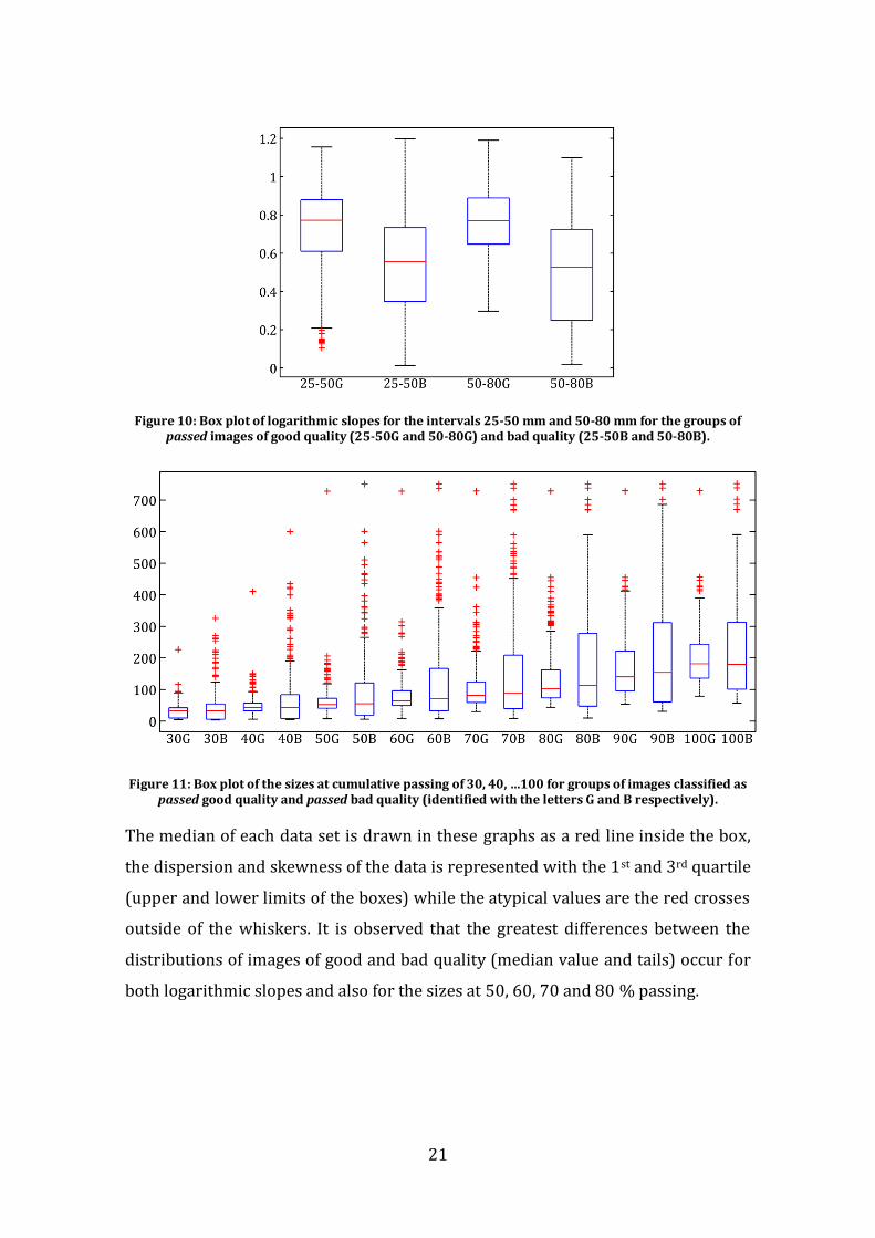
Figure 10: Box plot of logarithmic slopes for the intervals 25-50 mm and 50-80 mm for the groups of passed images of good quality (25-50G and 50-80G) and bad quality (25-50B and 50-80B).

Figure 11: Box plot of the sizes at cumulative passing of 30, 40, …100 for groups of images classified as passed good quality and passed bad quality (identified with the letters G and B respectively).

The median of each data set is drawn in these graphs as a red line inside the box,

the dispersion and skewness of the data is represented with the 1st and 3rd quartile

(upper and lower limits of the boxes) while the atypical values are the red crosses

outside of the whiskers. It is observed that the greatest differences between the

distributions of images of good and bad quality (median value and tails) occur for

both logarithmic slopes and also for the sizes at 50, 60, 70 and 80 % passing.

22

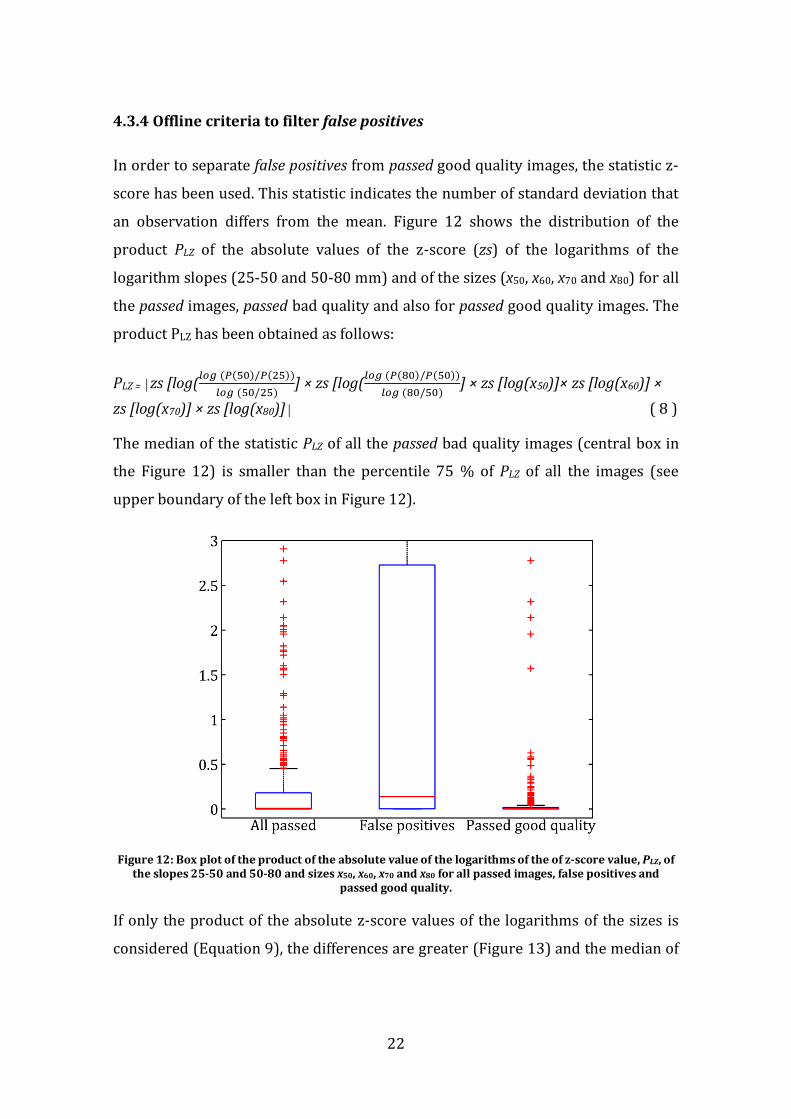
4.3.4 Offline criteria to filter false positives

In order to separate false positives from passed good quality images, the statistic z-

score has been used. This statistic indicates the number of standard deviation that

an observation differs from the mean. Figure 12 shows the distribution of the

product PLZ of the absolute values of the z-score (zs) of the logarithms of the

logarithm slopes (25-50 and 50-80 mm) and of the sizes (x50, x60, x70 and x80) for all

the passed images, passed bad quality and also for passed good quality images. The

product PLZ has been obtained as follows:

PLZ = │zs [log(

] × zs [log(

] × zs [log(x50)]× zs [log(x60)] ×

zs [log(x70)] × zs [log(x80)]│ ( 8 )

The median of the statistic PLZ of all the passed bad quality images (central box in

the Figure 12) is smaller than the percentile 75 % of PLZ of all the images (see

upper boundary of the left box in Figure 12).

Figure 12: Box plot of the product of the absolute value of the logarithms of the of z-score value, PLZ, of the slopes 25-50 and 50-80 and sizes x50, x60, x70 and x80 for all passed images, false positives and

passed good quality.

If only the product of the absolute z-score values of the logarithms of the sizes is

considered (Equation 9), the differences are greater (Figure 13) and the median of

23

the statistic PLZ of the passed bad quality images (central box - Figure 13) is above

of the percentile 75 % corresponding to all passed images (left box - Figure 13).

PLZ = │ zs [log(x50)] × zs [log(x60)] × zs [log(x70)] × zs [log(x80)]│ ( 9 )

Figure 13: Box plot of the product of the absolute value of the z-score logarithm, PLZ, of the x50, x60, x70 and x80 of all passed images, including good and bad quality, and good passed and bad. The green

rectangle indicates the deleted photos using the percentile 75 % (P75) of all passed images.

This means that if the passed images with a PLZ of the logarithm of the sizes x50, x60,

x70 and x80 over the percentile 75 % of this distribution are eliminated,

approximately half of the images with bad quality are also eliminated and only a

reduced amount of good quality images will be removed, as it is shown at Table 3.

Table 3: Passed images obtained at 11th,15th,16th and 17th of September, 2014. Results of filtering: percentile 75 % of the absolute product of the z-score of the logarithm of sizes x50, x60, x70 and x80.

Quality Code Description Images

Initial amount

Final amount

Deleted amount

Deleted percentaje

Passed good quality

0, 2 Good 288 267 21 7 1 Gray 95 89 6 6 9 Shadow 13 13 0 0

Passed bad quality

3, 4 Haul bed 68 48 20 29 5 Floor 119 44 75 63 6, 7 y 8 Others 113 61 52 46

Eliminated images

P75

24

In total, 147 passed bad quality images and 27 of good quality were deleted (see

Table 3). This leads to a ratio of passed images good to bad quality of 2,4:1.

Figure 14 shows the mean size distribution curves from the set of images under

analysis for all the passed images, passed images with good quality and retained

images after filtering. The fragmentation differences between all the passed photos

and only the ones with good quality is obvious, while the mean size distribution

curves of good quality images and retained images are very similar. Although it

was not possible to eliminate the total amount of false positive or passed bad

quality images, this result shows that the remaining bad quality curves do not

change significantly the results.

Figure 14: Mean size distribution curves for 11th, 15th, 16th and 17th September, 2014. Red line: all passed photos. Black line: passed good quality images. Blue: Remaining curves after filtering.

4.3.5 Results of the offline criteria

The proposed criteria eliminates the 50 % of the false positives images but also a

small percentage of the good quality images (less than the 10 %), in this way, the

Size (mm)

Pas

s (%

)

25

ratio good quality to bad quality is almost doubled from 1,32:1 to 2,4:1. It has been

shown that although an important amount of bad quality curves cannot be

eliminated, their effect on the mean size distribution could be considered as

limited.

Initially, this filter was used to the images captured each day, assuming that the

images of a whole day correspond to the same blast. Annex B shows the set of

curves obtained after filtering monthly. Table 4 summarizes the main

characteristics of the resulting size distributions after filtering; it shows the mean

and standard deviation (after the ± sign) for sizes at 20 %, 50 % y 80 % (x20, x50 y

x80) cumulative passing; it also shows the number of images retained (75 % of the

original total).

Table 4: Summary of the parameters of the curves filtered monthly.

No. images X20 X50 X80 September 2014 1284 8,8±1,8 67,2±30,6 142,9±77,7 October 2014 1267 8,8± 1,8 65,1±28,0 141,1±74,3 November 2014 133 8,3±2,5 76,0±85,8 140,1±109,3 December 2014 116 7,9±3,1 133,5±162,0 254,4±212,8 March 2015 61 9,4±1,9 169,0±173,9 296,0±202,1 April 2015 652 7,7± 2,1 51,7±22,5 106,1±52,3 May 2015 1556 8,4±2,0 59,3±26,1 121,5±67,6

Because the calculation was made monthly instead that for each blast, the results

have a large variability, and in some cases, the standard deviation is greater than

the mean. According to this result, the filter was applied to the images from each

blast individually when the loading dates were available.

4.3.6 Offline criteria application

Once the loading dates of each blasting were available, the size distribution curves

were grouped according to this criterion. This allowed analyzing fragmentation of

the blasts made from September 1st, 2014 to July 15th, 2015; during January and

February no image was recorded due to a connection problem. The images

26

allocated to each blast were filtered with the offline criteria described previously.

Table 5 shows the number of resulting images after filtering.

Table 5: Recorded images by blast.

Blast Total images post filtering



V1000 154 V823 196 V948 4 V1002 518 V824 105 V959 46 V1003 72 V825 193 V961 91 V1004 216 V828 208 V962 67 V1005 228 V829 106 V963 163 V1007 13 V835 325 V964 84 V1008 148 V841 79 V968 47 V1009 342 V845 149 V973 8 V1013 159 V851 57 V978 166 V1014 224 V854 78 V980 352 V1016 137 V860 10 V985 133 V420 220 V862 39 V987 404 V805 75 V867 10 V990 193 V806 68 V873 81 V991 28 V812 119 V934 16 V992 73 V815 201 V938 8 V995 358 V816 356 V945 17 V997 417

4.4 Fragmentation analysis

A total of 51 blasts have been analyzed. Annex C shows their main blast

parameters. The resulting fragmentation for each blast is assessed from the size at

cumulative passing of 80 %; the reason for using this size is that it is always larger

than the fines cut-off, 10 mm, and thus less affected by the errors in the

measurement (Sanchidrián et al., 2008). Figure 15 shows the boxplot of x80 sizes

for each blast; the large variability within data is apparent. The notches around the

median (or red line) of each set of data describes the 95 % confidence interval of

the median. It is necessary to take into consideration that if the notches from two

samples do not overlap, their x80 are different from a statistical point of view.

27

Figure 15: Boxplot of the x80 for each blast.

Figure 16 represents the relation between the median size x50 and x80. Most of the

points seem to follow a potential function type x80=a∙x50b (shown in green color); it

has been included the confidence limits of the fit values a and b, as well the

determination coefficient R2. The relation is not significant at a level of 95 %

confidence, i.e. the 95 % confidence interval of the fit constant a given in Figure 16

includes zero. The determination coefficient that shows the goodness of the fit is

high 0,865 though. This is likely caused by the leverage point at the upper left

corner of the graph.

28

Figure 16: Median size x50 versus x80 for the blast monitored in Cobre Las Cruces.

In order to determine which blasts have a different fragmentation it has been

applied the Wilcoxon Rank Sum test to the x80. The results are displayed in the

Table 6; p-values below 0,05 are in bold (they suggest that the fragmentation is

different from a statistical point of view).

According to this test, the number of blasts in which the fragmentation varies with

respect to each blast been calculated. Table 7 shows for this calculation the mean

number of blasts, the standard deviation, the minimum and the maximum, as well

as, the 25th, 50th and 80th percentiles. The same parameters are also shown as

percentage of the total. The 25th percentile, for instance, represents that a 25 % of

the blasts are different from 32 blasts out of 51, i.e. the 63 %, or less (see Table 7).

The fragmentation of blasts V938 and V1007 is different to 96 % of the blasts,

whereas fragmentation from blasts V860, V948 and V945 differs from the others in

only 8-9 blasts. It is remarkable that for all these five blasts, the number of

photographs was limited (V860 had 10, V938 had 8, V945 had 17, V948 had 4 and

V1007 had 13 images) compared to the rest of blasts (see Table 5).

x80= 1,13 · x50 0,89

R2= 0,865

a=[0,72; 1,54]

b=[ 0,79; 0,99]

29

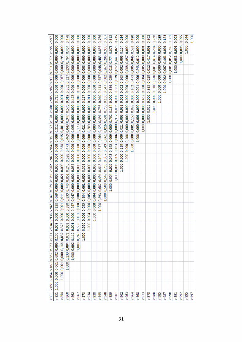
Table 6: P-value of x80 for the Wilcoxon Rank Sum test (the Table has been split in three pages to facilitate its reading).

32

Accordingly, if only blasts with more than 17 recorded images are considered, the

number of blasts different to each one is found in a range from 27 to 48 blasts.

Therefore, there is a significant fragmentation variation between the analyzed

blasts. These differences may be caused by the blast design parameters or/and the

rock mass characteristics.

Table 7: Disparity of x80 between blasts.

Mean Standard deviation

Minimum Maximum Percentile 25th 50th 75th

No. comparisons p-value <0.05

34 ± 8 8 49 32 35 39

% comparisons p-value <0.05

67 ± 16 16 96 63 69 76

One of the most relevant parameters to describe the blast characteristics is the

specific charge or powder factor (q) (Tosun, 2014), the amount of explosive used

per unit volume. The most widely model use to predict rock fragmentation by

blasting is the Kuz-Ram model developed by Cunningham (1987) based on the

Equation developed by Kuznetsov (1973) includes this parameter to predict the

median size of the fragmented rock:

( 10 )

Where:

is the median size (cm),

A is the rock factor,

q is the specific charge (kg/m3),

Q is explosive mass per hole (kg) and

RWS is relative weight strength respect to ANFO (generally the explosive energy is

assessed as heat of explosion).

33

The powder factor has together with the explosive energy the largest influence on

fragmentation and as the specific charge increases, the resulting fragmentation

size of a blast decreases through potential form. According to that, the powder

factor has been used, to analyze the effect of blasting on the resulting

fragmentation. The values of the x80 have been compared with the powder factor of

the blast (Figure 17). The relationship between both parameters is calculated as

follows x80=a∙qb (see green line in Figure 17) where q is the powder factor.

Although the fit is statistically significant, the determination coefficient is low, 0,28.

This result is affected by the influential point with a low powder factor (60 g/m3).

If this point is removed then the fit is not statistically significant and R2 takes

0,0005 as value.

Figure 17: Relationship between x80 and the specific explosive consumption.

Figure 18 shows the powder factor versus the bench level. Likewise, in the Figure

19 the x80 of each bench has been represented. The red circles represent the mean

of the x80 at each bench level. There were not images for bench -160, so no results

were obtained for it. In both cases no trend can be observed.

y=8,61· x -0,61

R2= 0,279

a=[6,801; 10,409]

b=[-0,892; -0,329]

34

Figure 18: Specific consumption versus its corresponding bench.

Figure 19: Resulting x80 of the blast performed in each bench.

35

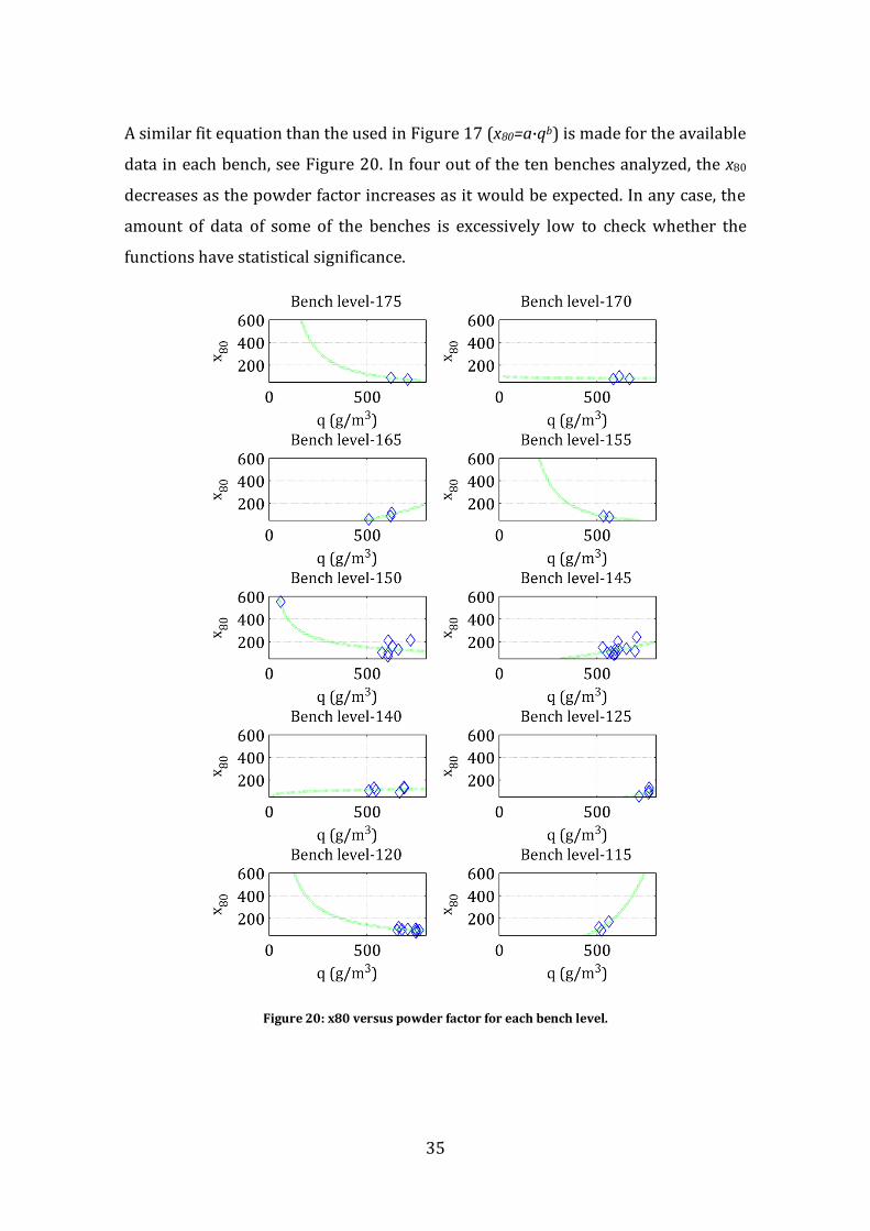
A similar fit equation than the used in Figure 17 (x80=a∙qb) is made for the available

data in each bench, see Figure 20. In four out of the ten benches analyzed, the x80

decreases as the powder factor increases as it would be expected. In any case, the

amount of data of some of the benches is excessively low to check whether the

functions have statistical significance.

Figure 20: x80 versus powder factor for each bench level.

36

Well-probed fragmentation models such as Kuznetsov model (1973), the Kuz-Ram

model by Cunningham (1987), and the Swebrec (Ouchterlony, 2005a) involve,

besides of characteristic parameters of the fragmentation distribution, a set of

parameters that include rock, drilling and blasting features. Thus, in order to

obtain more coherent results, other parameters which affect the fragmentation,

especially the rock properties (and consequently the rock factor) should be known.

On the other hand, the fact that the system has not been calibrated may contribute

to the large variability observed in Figure 17 between x80 and the powder factor.

The relevance of this action will be described in the next section.

37

5 Case study El Aljibe quarry

Split Online, was also installed in the quarry El Aljibe to monitor fragmentation

from six different blasts. A representative sample of the obtained images has been

also processed with Split Desktop to compare fully versus semi-automatic

delineation.

5.1 The site and fragmentation measurement system

The quarry El Aljibe is located in Almonacid de Toledo (Spain, see Figure 21). It

belongs to Benito Arnó e Hijos, S.A.U. and mines a mylonite deposit by drilling and

blasting to obtain railroad ballast (fraction 32/56 mm), and asphalt (6/12 mm

fraction). This metamorphic rock formed by tectonic forces, whose density is 2,68

t/m3, is very hard and tough. The mylonites have a porphyry-clastic texture with

potassium feldspar and plagioclase clasts encompassed in a matrix with biotite

foliation recrystallized in quartz crystals (Benito Arnó e Hijos, 2014). The strip of

mylonite of Toledo corresponds to a ductile shear zone, which was developed at

the end of the Hercynian Orogeny, 365 Myr. This shear zone separates migmatitic

rocks from Lower Paleozoic metasediments cover and granitic rocks.

Figure 21: El Aljibe quarry location, map and orthophoto.

Modified from IBERPIX Instituto Geográfico Nacional.

38

The annual production of run of mine is 0,5 Mt/year (data from 2012). Normally

one blast is loaded at each time. Figure 22 shows the flowsheet of the first part of

the processing plant. The run of mine is hauled directly by dump trucks to a

hopper with a grizzly of 120 mm. The grizzly bars are oblique with a separation

from 100 mm to 120 mm. It removes fragments below 120 mm from the flow of

the primary crusher. The passing material is further separated in two fractions by

a vibrating screen. The first group consists of fragments smaller than 25 mm which

are stored. The second one, fragments between 25-120 mm, is added to the

products of primary crusher (<170 mm) in a conveyor belt. These materials are

further processed depending on the requirements of the final product. The weights

of these size fractions are measured online with scale belts which provide the flow

rate in tons per hour and the accumulated tons; the location of these scales is

shown in Figure 22.

Figure 22: Primary phase of the crushing plant outline.

The camera of the fragmentation measuring system was placed over the grizzly,

focusing inside the feeder. This location allows assessing the effect of blasting on

the run of mine. The fact that most of fragments smaller than 120 mm passed

through the grizzly before the photographs have been taken leads to uniform size

distributions with fewer fines than the actual ones. The camera axis was kept

perpendicular to the surface to be photographed to obtain an exact image scaling.

The camera was triggered twenty seconds later that the flow rate of fragments

39

smaller than 120 mm is higher than 20 t/h (reading of scale S1) and the crusher

feeder is working. From that moment, the camera takes photos continuously with a

delay of eight seconds, until one of the two conditions are not fulfilled. The photos

are sent to the computer, where they were stored together with the readings of the

belt conveyors at the moment that a photograph was taken.

The belt scales provide the cumulative percentage of material at 25 and 120 mm.

These are calculated as follows:

P(25)= -

; P(120)=

( 11 )

Where Smj is the rock mass that passes through the belt scale Sj at a t time interval,

and T is the mass of processed material in that time window; it is calculated as

follows:

T=Sm1+Sm3-Sm2 ( 12 )

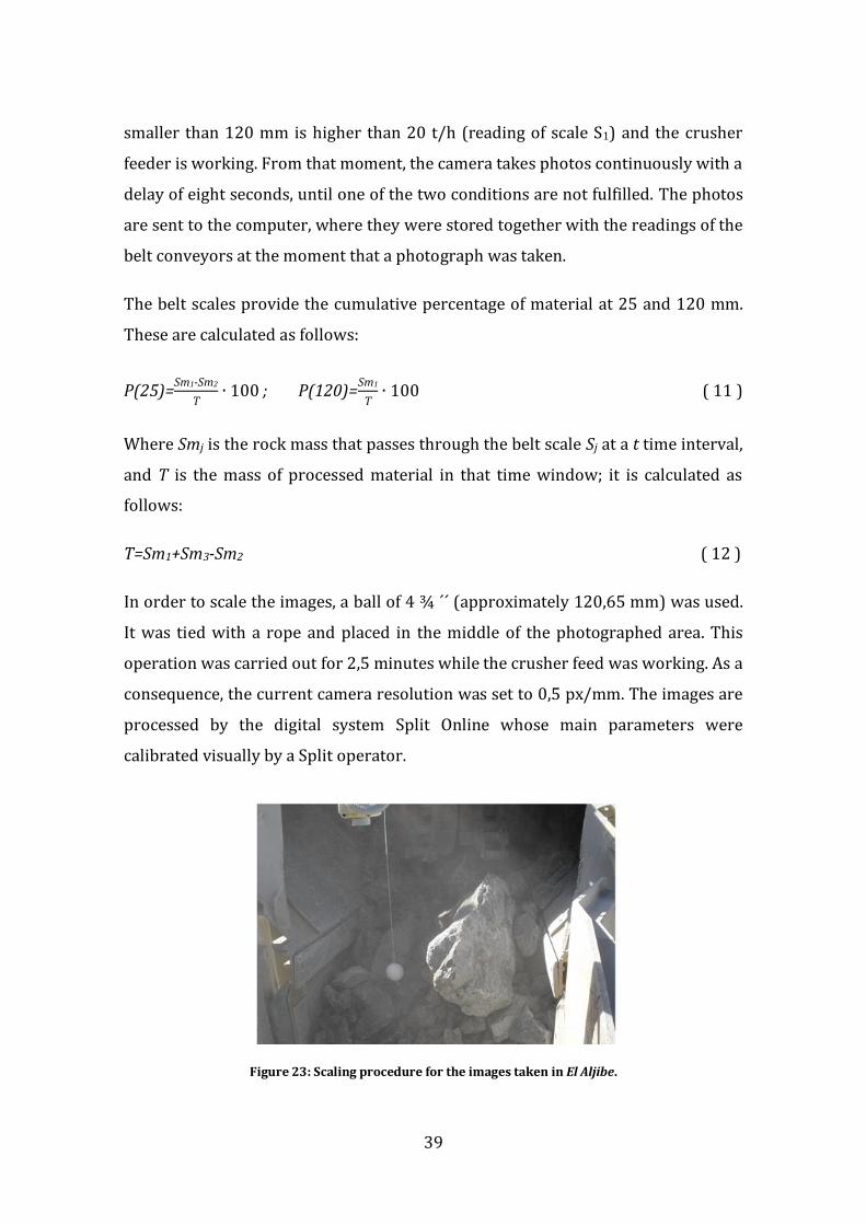
In order to scale the images, a ball of 4 ¾ ´´ (approximately 120,65 mm) was used.

It was tied with a rope and placed in the middle of the photographed area. This

operation was carried out for 2,5 minutes while the crusher feed was working. As a

consequence, the current camera resolution was set to 0,5 px/mm. The images are

processed by the digital system Split Online whose main parameters were

calibrated visually by a Split operator.

Figure 23: Scaling procedure for the images taken in El Aljibe.

40

5.2 Images identification

The system produces about 600 images per day which have to be assigned to each

blast. For this a set of production logs have been used:

- Perforation log: It is completed by the driller specifying the number of holes

drilled and the time needed to drill each hole.

- Loading log: It is completed by the shovel operator. It describes the blast

that is being loaded making possible to identify the images for each blast.

- Crusher log: It is completed by the primary crusher operator. It shows the

hour in which each truck dumps in the primary crusher.

5.3 The blasts

Table 8 shows the main characteristics of the monitored blasts; it gives mean and

standard deviation of the bench height (H), the burden (B), the spacing (S), the

borehole length (lB) and the subdrill length(ls). The geometrical parameters were

monitored with a Laser profile from MDL. When the sixth blast (B6) took place, the

quarry was flood by water (Figure 24), causing an error in the measurement of ls.

This is significatly deeper than the others (Table 8). For the fifth blast (B5) the

situation was quite similar.

Figure 24: Quarry conditions in blast B6.

Table 8 also shows the explosive mass per hole; the explosives used were bulk

ANFO and cartridged gelatine. The quantity of gelatine used depends on the

41

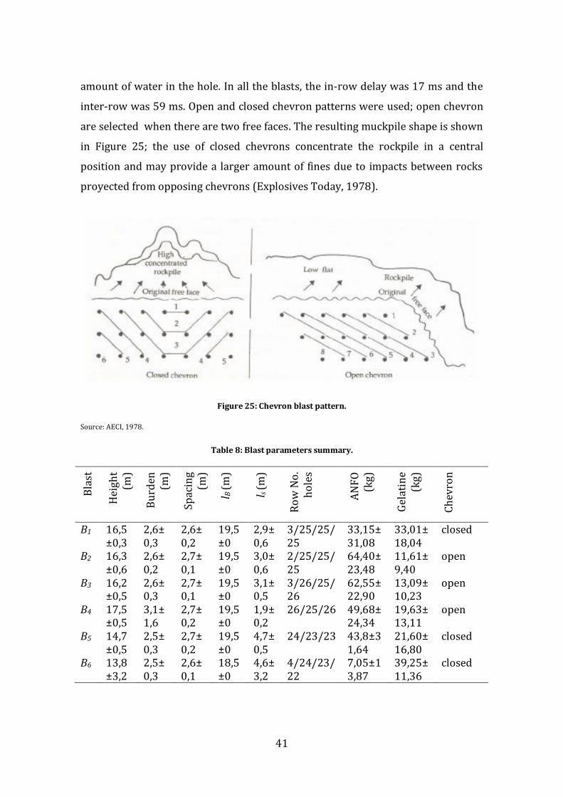
amount of water in the hole. In all the blasts, the in-row delay was 17 ms and the

inter-row was 59 ms. Open and closed chevron patterns were used; open chevron

are selected when there are two free faces. The resulting muckpile shape is shown

in Figure 25; the use of closed chevrons concentrate the rockpile in a central

position and may provide a larger amount of fines due to impacts between rocks

proyected from opposing chevrons (Explosives Today, 1978).

Figure 25: Chevron blast pattern.

Source: AECI, 1978.

Table 8: Blast parameters summary.

Bla

st

Hei

gh

t (m

)

Bu

rden

(m

)

Spac

ing

(m

)

l B (

m)

l s (

m)

Ro

w N

o.

ho

les

AN

FO

(k

g)

Gel

atin

e (k

g)

Ch

evro

n

B1 16,5±0,3

2,6±0,3

2,6±0,2

19,5±0

2,9±0,6

3/25/25/25

33,15±31,08

33,01±18,04

closed

B2 16,3±0,6

2,6±0,2

2,7±0,1

19,5±0

3,0±0,6

2/25/25/25

64,40±23,48

11,61±9,40

open

B3 16,2±0,5

2,6±0,3

2,7±0,1

19,5±0

3,1±0,5

3/26/25/26

62,55±22,90

13,09±10,23

open

B4 17,5±0,5

3,1±1,6

2,7±0,2

19,5±0

1,9±0,2

26/25/26 49,68±24,34

19,63±13,11

open

B5 14,7±0,5

2,5±0,3

2,7±0,2

19,5±0

4,7±0,5

24/23/23 43,8±31,64

21,60±16,80

closed

B6 13,8±3,2

2,5±0,3

2,6±0,1

18,5±0

4,6±3,2

4/24/23/22

7,05±13,87

39,25±11,36

closed

42

In order to obtain the volume of each blasted block of material, the data from laser

profile is used. The shape of the block is resembled to a parallelepiped. The

horizontal surface was calculated between the curve formed by the median of

scanned bench face and the last row of boreholes line both in top view. The volume

is estimated multiplying the average height of the bench by its surface. Once the

volume is known, it is possible to calculate the powder factor or specific charge (q).

Due to the huge variability of subrill, the powder factor above grade (qf) is

considered. These data are shown in Table 9.

Table 9: Specific charge.

Blast Volume (m3) Explosives (kg) q (kg/m3) Explosivesf (kg) qf (kg/m3) B1 10 037,0 5 161 0,51 3,556 0,35 B2 9 593,1 5 853 0,61 4,209 0,44 B3 10 066,0 6 042 0,6 4,283 0,43 B4 11 431,0 5 336 0,47 4,236 0,37 B5 7 603,4 4 578 0,6 2,321 0,31 B6 6 477,0 3 380 0,52 1,746 0,21

The powder factor above grade qf decreases with respect to q especially in those

blast which had an excessive subdrill such as blasts B5 and B6. The explosive in the

subdrilled part of the hole (difference between q and qf) it is mainly used to break

toe and has a limited effect on rock fragmentation.

5.4 Fragmentation measurements

Split Online delineates the edge of each fragment automatically generating the size

distribution curves, which are volume-based (as was explained in Section 3.1). A

total of 21 834 images corresponding to six blasting has been analyzed by this

system (an average of 3.639 pictures per blast, from 1 626 to 5 369). Because of

the camera resolution it is not possible to measure sizes smaller than 32 mm,

which is the fines cut-off. This is shown in Figure 26, where size distribution curves

from the first blast B1 are plotted. At sizes smaller than 32 mm all curves become

parallel as the system extrapolates the fine tail, using the underlying distributions

43

described in section 3.1. Fragmentation data below this size is not considered in

this work.

Figure 26: Size distribution curves from blast B1.

Whenever a photograph is processed by Split Online software, the program

provides the cumulative passing P(x), for the already defined mesh series x. It also

gives the sizes xP at a passing P from 10 to 100 in steps of 10 %. For each photo, the

size distribution curve is built from these data; see as an example Figure 27.

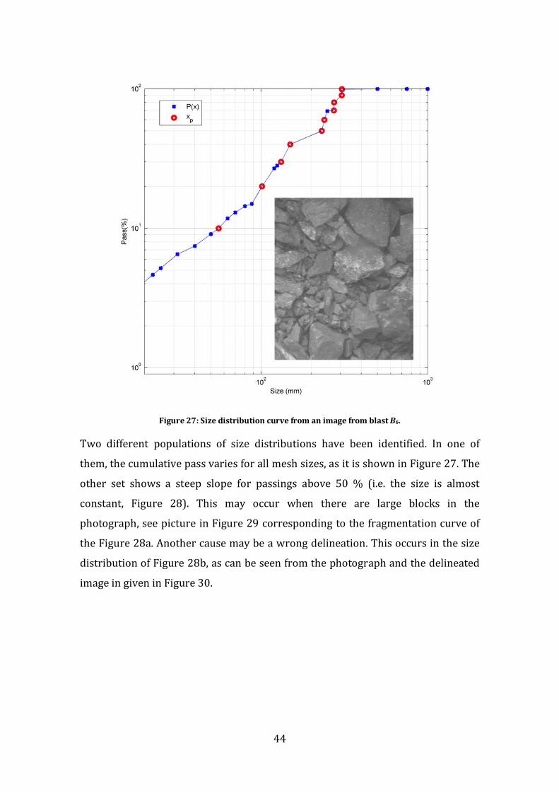
44

Figure 27: Size distribution curve from an image from blast B6.

Two different populations of size distributions have been identified. In one of

them, the cumulative pass varies for all mesh sizes, as it is shown in Figure 27. The

other set shows a steep slope for passings above 50 % (i.e. the size is almost

constant, Figure 28). This may occur when there are large blocks in the

photograph, see picture in Figure 29 corresponding to the fragmentation curve of

the Figure 28a. Another cause may be a wrong delineation. This occurs in the size

distribution of Figure 28b, as can be seen from the photograph and the delineated

image in given in Figure 30.

45

Figure 28: Size distribution curves of images with a few large fragments (a) or with a wrong delineation (b).

Figure 29: Photograph and delineation of curve 28a.

Figure 30: Photograph and delineation of curve 28b.

5.4.1 Reliability respect to fines cut-off

Due to the fact that the closer to fines cut-off, the larger the measuring errors are

(Sanchidrián et al., 2008), the difference from the mean of the passing values in

each blast to the fines cut-off has been calculated. The passing values vary from

28b 28a

46

three times the fines cut-off for finest sizes to twelve times for the largest.

According to Sanchidrián et al., 2008 at sizes greater than the fines cut-off the

delineation calculation provides measurements with a maximum of error of 30 %,

so even the lowest passing, x10, may be reliable. Figure 31 shows the sizes at

passings of 20, 50 and 80 % identified as x20, x50 and x80, respectively. It also shows

the percentage of material that pass through the sieve P(25) (see Figure 22),

cumulative passing at fines cut-off size P(32), and cumulative passing that not pass

through the grizzly P(120) (see Figure 22).

Figure 31: Boxplot of the whole set of images per each blast (note that the scales of the ordinates axis are different in each graph).

5.4.2 Semi-automatic analysis of fragmentation

As a limited number of images can be analyzed reasonably in semi-automatic mode

twenty photos are randomly sampled from the whole set of images assigned to a

blast.

Consequently, it has been checked first whether the samples randomly selected are

representative of the whole fragmentation of the blast. For the analysis, instead of

working with the complete size distribution data, only the sizes x80, x50 and x20 are

P(25) P(32) x20 x50 x80 P(120)

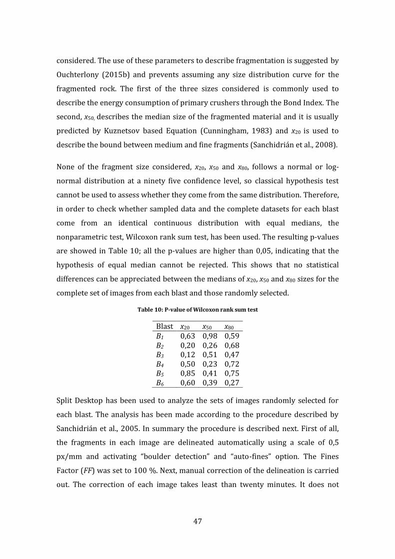
47

considered. The use of these parameters to describe fragmentation is suggested by

Ouchterlony (2015b) and prevents assuming any size distribution curve for the

fragmented rock. The first of the three sizes considered is commonly used to

describe the energy consumption of primary crushers through the Bond Index. The

second, x50, describes the median size of the fragmented material and it is usually

predicted by Kuznetsov based Equation (Cunningham, 1983) and x20 is used to

describe the bound between medium and fine fragments (Sanchidrián et al., 2008).

None of the fragment size considered, x20, x50 and x80, follows a normal or log-

normal distribution at a ninety five confidence level, so classical hypothesis test

cannot be used to assess whether they come from the same distribution. Therefore,

in order to check whether sampled data and the complete datasets for each blast

come from an identical continuous distribution with equal medians, the

nonparametric test, Wilcoxon rank sum test, has been used. The resulting p-values

are showed in Table 10; all the p-values are higher than 0,05, indicating that the

hypothesis of equal median cannot be rejected. This shows that no statistical

differences can be appreciated between the medians of x20, x50 and x80 sizes for the

complete set of images from each blast and those randomly selected.

Table 10: P-value of Wilcoxon rank sum test

Blast x20 x50 x80 B1 0,63 0,98 0,59 B2 0,20 0,26 0,68 B3 0,12 0,51 0,47 B4 0,50 0,23 0,72 B5 0,85 0,41 0,75 B6 0,60 0,39 0,27

Split Desktop has been used to analyze the sets of images randomly selected for

each blast. The analysis has been made according to the procedure described by

Sanchidrián et al., 2005. In summary the procedure is described next. First of all,

the fragments in each image are delineated automatically using a scale of 0,5

px/mm and activating “boulder detection” and “auto-fines” option. The Fines

Factor (FF) was set to 100 %. Next, manual correction of the delineation is carried

out. The correction of each image takes least than twenty minutes. It does not

48

worth doing in a very thorough manner due to each particle has a scarce influence

on the fragmentation size curve. Consequently, the main aspects are to correct the

large blocks which were divided in several smaller in the delineation, to join those

which were separated in packets of fines and to hide the areas of the image that

the operator do not desire to use for the calculation.

The resulting size distribution curves are shown in Figure 32. It also shows the

resulting fragmentation from Split Online for the same images. The size

distribution curves for both measurement systems are drawn including all the data

provided by the software mentioned in section 5.4, i.e. the cumulative passing P(x),

for the defined mesh series x, and sizes xP at a passing P from 10 to 100 in steps of

10 %. Due to the fact that the mesh was not the same for all the images, the median

of the curves (red and black lines) are calculated using only the sizes xP at a passing

P from 10 to 100 in steps of 10 %. In order to check whether the medians of the

sizes x20, x50 and x80 for each blast from the automatic and semi-automatic analysis

are different, the Wilcoxon rank sum test has been applied. The p-values are shown

in the Table 11; values above 0,05 are marked in bold. They show that no

statistical differences can be assessed between both analysis modes.

Table 11: P-value of Wilcoxon rank sum test for Split Online and Split Desktop curves.

Blasting x20 x50 x80 B1 <0,01 <0,01 <0,01 B2 <0,01 <0,01 0,06 B3 <0,01 <0,01 <0,01 B4 <0,01 0,12 0,26 B5 <0,01 0,07 0,80 B6 0,13 0,08 0,21

The results provided mean that only for one blasting, B6, the three sizes x20, x50, and

x80 from automatic and semi-automatic analysis are comparable. For blasts B2, B4

and B5 only the upper part of the curve does not varies, but the medians of all sizes

are statistically different in blasts B1 and B3.

49

Figure 32: Fragmentation from Split Online (automatic mode) and Split Desktop (semi-automatic mode) of the sets of 20 images randomly selected for each blast (Blue lines: Split Online, cyan lines:

Split Desktop, black line: Split Online median, red line: Split Desktop median).

50

The median of the sizes x20, x50, and x80 from automatic and semi-automatic

analysis are plotted in Figure 33. The following linear fit has been made:

xSOL = a + b·xDSM ( 13 )

Where a and b are coefficient estimates for a linear regression of the responses in

f(x) on the predictors in x, i.e. mesh size of Split Online (xSOL) and Split Desktop

(xSD). The closer is R2 to the unit, the more accurate is the fit.

Table 12 shows the results of the fit. The fitted lines are also shown with a red line

in Figure 33. The line passing through the origin with a slope of one is plotted in

black as a reference.

Figure 33: Plot of different sizes from Split Online and Split Desktop.

The 95 % confidence intervals of the coefficient estimated indicates if the results

are meaningful. Ideally xSOL must be equal to xSD. This involves that the 95 %

confidence interval of a must comprise zero, and the interval for b must embrace

one. The determination coefficient, R2, shows the goodness of the fit. The closer is

R2 to the unit, the more accurate is the fit.

Table 12: Fit parameters for Split Online versus Split Desktop.

Coefficient estimated 95 % confidence intervals R2

x20 a= 135,96 [109,41; 162,51] 0,6878 b= 0,24 [0,015; 0,47]

x50 a= 188,81 [117,45; 260,18] 0,7790 b= 0,43 [0,11; 0,75]

x80 a= 335,15 [161,30; 509,00] 0,5028 b= 0,18 [-0,32; 0,69]

51

The use of automatic analysis causes a systematic error in the measurements (a

confidence interval does not include zero), and in general the resulting sizes are

coarser than those given by the manual correction. In addition, the fit is not

statistically meaningful for the coarsest size, i.e. no linear relation can be assessed

for x80 (b confidence interval includes zero).

5.5 Correction procedure of fragment size distribution curves

The median fragment size distribution curve of each blast must be corrected due to

the fact that most of fines (below 120 mm) do not appear in the photos because

they were taken over the grizzly (see Figure 22). The measurements from the

three belt scales are used for this purpose. In order to do this correction, the first

step is to calculate the increment of the cumulative percentage at each size. For the

k Bin, this is:

Bin*k = -

( 14 )

Where P*k is the cumulative passing original at size k, being k=1 the smallest size.

Obviously, is equal to

. The correction is performed in three sections:

- Sizes lower or equal to 25 mm. The bins are corrected in this form:

Bink=

( 15 )

Where P25 is the cumulative passing at 25 mm given for that blast by the belt

scales.

- Sizes bigger than 25 and lower or equal to 120 mm:

Bink= -

-

( 16 )

Where P120 is the cumulative passing at 120 mm given for that blast by the belt

scales

52

- Sizes bigger than 120 mm:

Bink= -

-

( 17 )

With all k Bins calculated, the cumulative passing corrected for each sizes is

achieved by:

Pk= = ( 18 )

Figure 34 shows the results of applying this correction to the median Split Online

(SOL) and Split Desktop (SD) size distribution curves for the twenty images

sampled for each blast. In the section between P25 and P120, fragmentation is very

similar for both modes of delineation.

53

Figure 34: The median size distribution curves of Split Online (SOL) and Split Desktop (SD) and its correction by scale belt values (SOLc and SDc).

54

Similarly to what was performed in the section 5.4.2., the median sizes x20, x50, and

x80 resulting from the calibration of the automatic and semi-automatic analysis are

plotted in Figure 35. The results from the linear fit according to the Equation 13

are also plotted (red line) including a black line with slope one as a reference. The

results of the fitting are shown in Table 13.

Figure 35: Plot of different sizes from Split Online corrected and Split Desktop corrected.

The Split Online and Split Desktop values have shifted to a closer position

compared to the original values (before correction). However, the fitting results

reveal that the calibration of the system by the belt scales do not produce a

relevant convergence for SOL and SD. The sizes x20 obtain the better convergence

due to the fact that they are closer to the sizes that the belt scales measures (P25

and P120), so the effect of the correction at these points is most influential. For the

same reason, the relation of SOL and SD is only statistically meaningful at x20 as a

confidence interval includes zero and b confidence interval embraces one (R2 in

bold in Table 13).

Table 13: Fit parameters for Split Online corrected versus Split Desktop corrected.

Coefficient estimates 95 % confidence intervals R2

x20 a= -8,40 [-36,28; 19,47] 0,8383 b= 1,45 [0,56; 2,33]

x50 a= 150,42 [17,31; 283,54] 0,4770 b= 0,45 [-0,20; 1,10]

x80 a= 375,72 [309,69; 441,75] 0,1623 b= 0,06 [-0,13; 0,26]

55

5.5.1 Effect of blasting in fragmentation

Three sizes are considered to the fragmentation analysis. These are the sizes at 20,

50, and 80 % of the corrected size distributions from automatic and semi-

automatic analysis. As it was mentioned in the section 4.5, the effect of the blasting

is explained through the powder factor. This affect to the resulting fragmentation

(Cunningham, 1983), so for each size the following fit has been analyzed:

log(xk) = a·log(qf)b ( 19 )

Where qf is the powder factor above grade. The use of the powder factor above

grade instead of the powder factor was justified in the section 5.3. Table 14

summarizes the fitting results to Split Online (SOL) and Split Desktop (SD) which

are plotted in Figure 36.

Table 14: Regress parameters following log(xk)=a·log(x)b for powder factor above grade.

a a interval b b interval R2 SOL x20 1,79 [0,16 3,43] -1,52 [-3,00 -0,03] 0,6680 x50 5,32 [5,14 5,50] -0,15 [-0,32 0,01] 0,6269 x80 5,94 [5,88 5,99] -0,04 [-0,09 0,01] 0,5922 SD x20 2,21 [0,65 3,77] -1,03 [-2,45 0,39] 0,5049 x50 4,95 [4,79 5,12] -0,37 [-0,49 -0,19] 0,9054 x80 5,43 [5,07 5,80] -0,36 [-0,69 -0,03] 0,6954

The regression will be more accurate if R2 takes a large value. It will be meaningful

if the zero is not included in 95 % confidence intervals of the fitting constants a

and b interval. This occurs for the three fits: one given by automatic analysis SOL,

x20, and two given by the manual edition SD, x50 and x80; the determination

coefficients of these fits are marked in bold in Table 14. The values at B6 are a

leverage point in most of the cases with a large influence in the results, mainly on

the SOL fits. For x50 and x80 given by semi-automatic analysis, the powder factor

from B5 is in the middle range reducing the effect of B6. In order to evaluate the

influence of B6, it has been accomplished the equivalent fit excluding it. The results

are also drawn in Figure 36 (red line) and the fit parameters are shown in Table

15. When B6 is ignored the fit is statistically meaningful only for x50 of Split

Desktop.

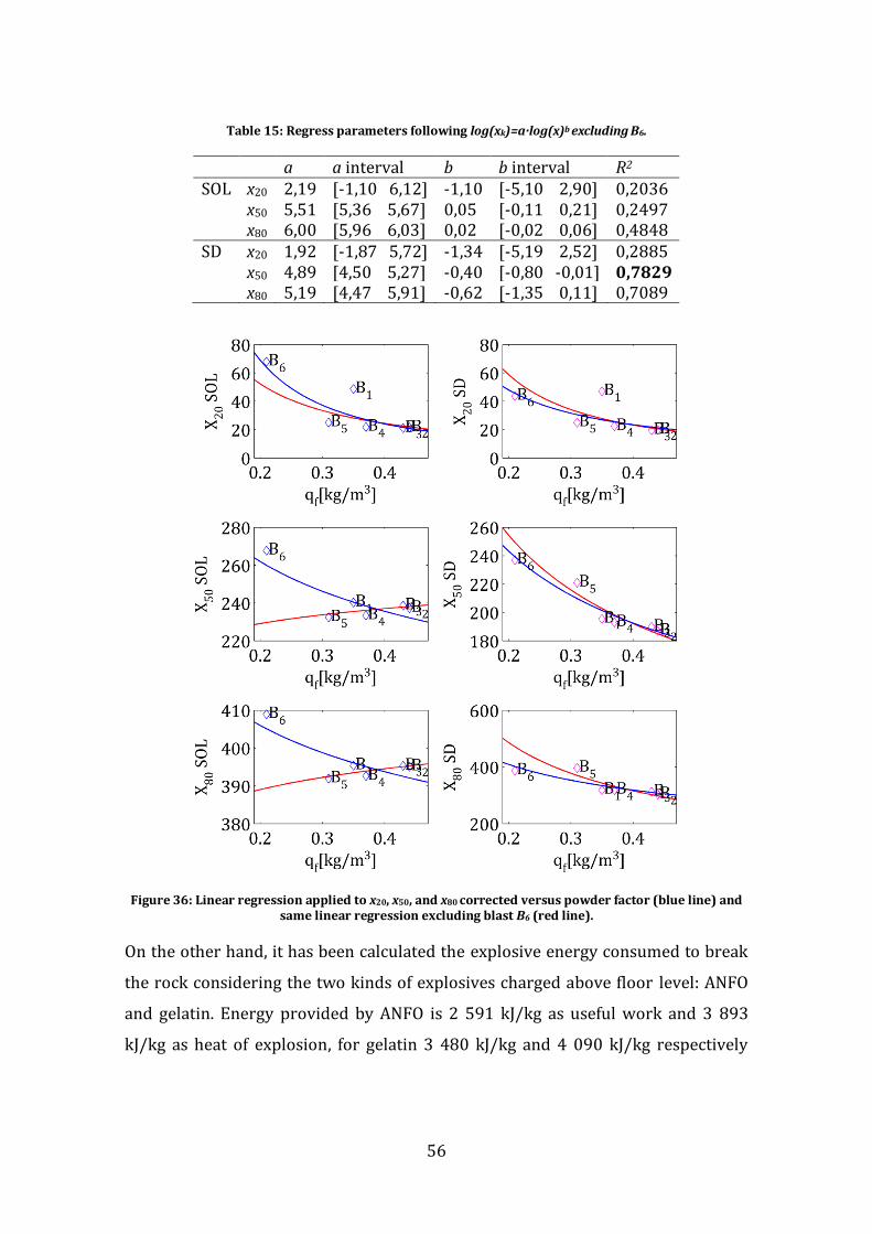
56

Table 15: Regress parameters following log(xk)=a·log(x)b excluding B6.

a a interval b b interval R2 SOL x20 2,19 [-1,10 6,12] -1,10 [-5,10 2,90] 0,2036 x50 5,51 [5,36 5,67] 0,05 [-0,11 0,21] 0,2497 x80 6,00 [5,96 6,03] 0,02 [-0,02 0,06] 0,4848 SD x20 1,92 [-1,87 5,72] -1,34 [-5,19 2,52] 0,2885 x50 4,89 [4,50 5,27] -0,40 [-0,80 -0,01] 0,7829 x80 5,19 [4,47 5,91] -0,62 [-1,35 0,11] 0,7089

Figure 36: Linear regression applied to x20, x50, and x80 corrected versus powder factor (blue line) and same linear regression excluding blast B6 (red line).

On the other hand, it has been calculated the explosive energy consumed to break

the rock considering the two kinds of explosives charged above floor level: ANFO

and gelatin. Energy provided by ANFO is 2 591 kJ/kg as useful work and 3 893

kJ/kg as heat of explosion, for gelatin 3 480 kJ/kg and 4 090 kJ/kg respectively

57

(Sanchidrián et al., 2006). From these data the specific energy eWu and eq are

calculated, respectively (Table 16).

Table 16: Useful work and heat of explosion energy.

Blast Gelatin (kg) ANFO (kg) eWu (KJ/m3) eq (KJ/m3) B1 1765 1790 1074 1414 B2 63 4146 1143 1709 B3 161 4122 1117 1660 B4 926 3310 1032 1459 B5 412 1908 839 1199 B6 1746 0 938 1103

With this values, it has been drawn the relationship between x20, x50 and x80 and ewu

and eq. Additionally a power fit type using Equation 19 has been made and shown

in Figure 37 and Figure 38. The results of each fit are shown in Table 17 and Table

18 respectively. For both specific energy types, eWu and eq, the fit is statically

meaningful for the sizes x50 and x80 obtained after manual edition of the photos. It

seems that the calibration at lower sizes 25 and 120 mm does not correct the

errors caused by the delineation at coarse size fractions.

Table 17: Regress parameters for specific useful work energy eWu.

a a interval b b interval R2 SOL x20 3,45 [2,82 4,06] -1,19 [-6,92 4,54] 0,0766 x50 5,49 [5,42 5,55] -0,07 [-0,68 0,54] 0,0252 x80 5,98 [5,96 6,00] -0,02 [-0,20 0,16] 0,0184 SD x20 3,33 [2,85 3,82] -0,92 [-5,40 3,57] 0,0746 x50 5,33 [5,26 5,39] -0,69 [-1,31 -0,07] 0,7053 x80 5,84 [5,79 5,88] -0,95 [-1,39 -0,54] 0,9095

Table 18: Regress parameters for specific heat of explosion energy eq.

a a interval b b interval R2 SOL x20 4,10 [3,01 5,20] -2,01 [-4,91 0,90] 0,4782 x50 5,54 [5,41 5,67] -0,17 [-0,52 0,18] 0,3156 x80 6,00 [5,96 6,09] -0,05 [-0,15 0,06] 0,2820 SD x20 3,82 [2,92 4,72] -1,47 [-3,86 0,92] 0,4223 x50 5,49 [5,41 5,58] -0,53 [-0,75 -0,31] 0,9197 x80 6,03 [5,91 6,16] -0,68 [-0,97 -0,29] 0,8670

The same comparison between SOL data after correction and the specific charge

and specific heat of explosion was also made including the whole data set of Split

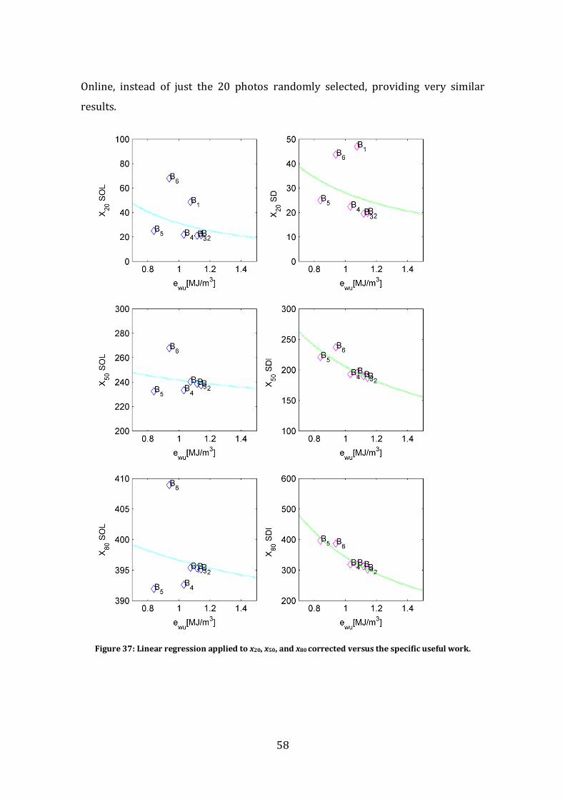
58

Online, instead of just the 20 photos randomly selected, providing very similar

results.

Figure 37: Linear regression applied to x20, x50, and x80 corrected versus the specific useful work.

59

Figure 38: Linear regression applied to x20, x50, and x80 corrected versus specific heat of explosion.

60

6 Conclusions

The digital image analysis performance of Split Online (automatic) to measure fine

and coarse fragmentation have been assessed. Fragmentation has been measured

in 51 blasts in Cobre las Cruces mine and in 6 more blasts obtained in El Aljibe

quarry. In Cobre las Cruces fragmentation has been measured over the trucks that

haul ore to the homogenizing muckpiles, whereas in El Aljibe the images were

taken over the grizzly of 120 mm of the primary crusher. Consequently the

majority of the particles smaller than this size were not included. In El Aljibe

fragmentation is significantly coarser than in Cobre las Cruces and therefore easier

to analyse by image based methods, i.e. most fragments are reasonably above the

resolution of the system and manual correction of the delineation is more accurate

because the operator can observes the actual size.

The main findings of this work are:

1) An offline criterion to discard false positives, (i.e. images analysed by the

system that do not include blasted rock) has been designed. This filter

allows rejecting 50% false positives while only 10% of good quality images

were discarded. The retained false positives have a negligible influence in

the resulting mean size distribution.

2) Fragmentation measurements with Split Online, automatic delineation, in

Cobre las Cruces mine without any calibration are no sensitive to changes in

the powder factor. The fact that the overall fragmentation size was fine

(median of size x50 equal to 54 mm), and therefore more prone to errors,

could be the source of this result.

3) Results from Cobre las Cruces show that the mean fragmentation depends

on the number of images analysed due to the fact that the less images the

higher is the effect of each photography. This is a limitation in

fragmentation studies based on few images per blast.

4) In El Aljibe, the performance of the automatic analysis of Split Online has

been assessed. Delineation of 20 images per blast randomly selected has

been manually edited (semi-automatic edition). The automatic analysis

61

shows a coarser fragmentation and a systematic error compared with those

from semi-automatic analysis in statistic terms.

5) Fragmentation measured in El Aljibe has been corrected to include fines

fractions from belt scale measurements at 25 and 120 mm. As this

corresponds to a passing below 20 % of the total blasted material,

calibration is then limited to the fines. Measurements of coarse sizes, like

x50 and x80, depend on the success of the delineation algorithms.

6) x20 measured by Split Online in El Aljibe presents a meaningful relation with

respect to the specific charge, but not with the specific energy. A random

effect due to the limited number of considered blasts and a leverage point in

the fit (blast B6) may be the reason behind this result. In contrast the

sizes x50 and x80 obtained from semi-automatic analysis are sensitive to the

powder factor above grade and specific energy. This result is consistent

with the role of these parameters on fragmentation.

7) Only medium and coarse sizes (such x50 and x80) from semi-automatic

analysis, once the correction has been made, shows a meaningful relation

with either the powder factor above grade or the specific energy; the

resulting determination coefficients are good from 0,7 to 0,92, but more

data is required to get a definitive conclusion.

62

7 References

AECI (1978): “Blasthole drilling and initiation patterns in surface blasting”.

Explosives Today. Series 2. No. 12: June, 1978.

Banner Engineering Corp.: “R-GAGE TM QT50R-AFH Sensor manual”.

Benito Arnó E Hijos, SAU. (2014): “Pedrera El Aljibe”. www.arno.es at 17

June 2016.

Cunningham C. V. B. (1983): “The Kuz-Ram model for prediction of

fragmentation from blasting. Holmberg R, Rustan A (eds) Proceedings of the

first international symposium on rock fragmentation by blasting. Luleå

University of Technology, Sweden, pp. 439-453.

Cunningham C. V. B. (1987): “Fragmentation estimations and the Kuz-Ram

model – for years”. 2nd International Symposium on Rock Fragmentation in

Blasting. Keystone, Colorado, USA, pp. 475-487.

Doyle, M., Ovejero, G. (2002): “Actas del XI Congreso Internacional de

Industria, Minería y Metalurgia, Zaragoza”.

Espí, J., Contreras, J. (2010): “La Huella del Carbono en la clasificación

ambiental de los proyectos mineros: Cobre Las Cruces (España)”.

IBERPIX. “Ortofotos Y Cartografía Raster." Instituto Geográfico Nacional.

Centro Nacional de Información Geográfica. Ministerio de Fomento.

Gobierno de España. www.ign/iberpix 17 June 2016.

Kemeny, J., Girdner, K., Bobo, T. and Norton, B. (1999). “Improvements for

fragmentation measurement by digital imaging: Accurate estimation of

fines”. Proc. 6th Int. Symposium on Rock Fragmentation by Blasting, pp. 8-

12 August, Johannesburg, The South African Institute of Mining and

Metallurgy, Johannesburg, pp 103-109.

Kuznetsov, V. M. (1973): “The mean diameter of the fragments formed by

blasting rock”. Soviet Mining Science, 9, 144-148.

Latham, J. P., Kemeny, J., Maerz, N., Noy, M., Schleifer, J., Tose, S. (2003): “A

blind comparison between results of four image analysis systems using a

63

photo-library of piles of sieved fragments”, Int. J. Blasting Fragment. 7–2,

105–132.

Moser, P. (2003): “Les fines production in aggregate and industrial minerals

industry”. Explosives and blasting technique, Holmberg (ed.). Swets &

Zeitlinger, Lisse.

Palangio, T. C., Maerz, N. H., (1999): “Case studies using the WipFrag image

analysis system”. FRAGBLAST 6, Sixth International Symposium For Rock

Fragmentation By Blasting, Johannesburg, South Africa, Aug. 8-12 1999, pp.

117-120.

Onederra, I., Esen S. and Jankovic A. (2004): “Estimation of fines generated

by blasting – applications for the mining and quarrying industries”. Mining

Technology (Trans. Inst. Min. Metall. A) December 2004 Vol. 113

Ouchterlony, F. (2003): “Influence of blasting on the size distribution and

properties of muckpile fragments, a state of the art review”. Swebrec, Lulea

University of Technology.

Ouchterlony, F. (2005a): “The Swebrec function: linking fragmentation by

blasting and crushing. Minig Technology (Trans. Inst. Min. Metall. A) Vol.

114.

Ouchterlony, F. (2005b): “The Case for the Median Fragment Size as a Better

Fragment Size Descriptor than the Mean”. Rock Mechanics and Rock

Engineering. Volume 49, Issue 1, pp. 143-164.

Sanchidrián, J., Segarra, P., López, L. (2005): “A Practical Procedure for the

Measurement of Fragmentation by Blasting by Image Analysis”. Springer-

Verlag.

Sanchidrián, J., Segarra, P., López, L. (2006): “Energy components in rock

blasting”. International Journal of Rock Mechanics and Mining Sciences.

Volume 44, Issue 1, January 2007, pp. 130–147.

Sanchidrián, J., Segarra, P., Ouchterlony, F., López, L. (2008): “On the

accuracy of fragment size measurement by image analysis in combination

with some distribution functions”. Rock Mechanics and Rock Engineering.

February 2009, Volume 42, Issue 1, pp. 95–116.

http://www.sciencedirect.com/science/journal/13651609

http://www.sciencedirect.com/science/journal/13651609/44/1

http://link.springer.com/journal/603

http://link.springer.com/journal/603/42/1/page/1

64

Schleifer, J., Tessier, B. (2002): “Fragmentation assessment using the

FragScan system: Quality of a blast”. European Federation of Explosives

Engineers in Explosives and Blasting Technique -World Conference-; pp.

111-116; World conference on explosives & blasting technique. A Balkema,

Rotterdam.

Split Engineering (2001): “Manual de instrucciones Split-Net”. Split

Engineering LLC, Tucson, Arizona.

Tosun, A., Konak, G., Toprak, T. (2014): “Development of the kuz-ram model

to blasting in a limestone quarry”. Arch. Min. Sci., Vol. 59, No 2, pp. 477–488.

7.1 Further reading

Bel-lan, A., Locutura, J., Chamorro, M., Martínez, S. (2007): “Investigación y

estudios metodológicos sobre las técnicas geoquímicas y sus aplicaciones”.

Instituto Geológico y Minero de España (IGME).

Cobre las Cruces (2012):”Areas y procesos”. www.cobrelascruces.com, at 15

April 2016.

Hernández-Enrile, J. L. (1981): “Evolución microstructural de rocas cuarzo-

feldespáticas como resultado del aumento de la deformación en la milonita

de Toledo”. Universidad Complutense de Madrid.

Maerz, N. H., and Zhou, W., (1998): “Optical digital fragmentation measuring

systems - inherent sources of error”. FRAGBLAST, The International Journal

for Blasting and Fragmentation, Vol. 2, No. 4, pp. 415-431.

Rosin P., Rammler E., (1933): “The laws governing the fineness of powdered

coal”. J. Inst. Fuel, (7), pp. 29-36.

Strelec, S., Gazdek, M., Mesec J. (2011): “Blasting design for obtaining

desired fragmentation”. Technical Gazette 18, 1, pp. 79-86.

Segarra, P. (2004): “Análisis experimental de la fragmentación, vibraciones

y movimiento de la roca en voladuras a cielo abierto”. Doctoral Thesis,

Escuela Técnica Superior de Ingenieros de Minas, Madrid.

Soft-Blast (2006) University of Queensland.

https://www.tib.eu/en/search/?tx_tibsearch_search%5Bquery%5D=person%3A%28Schleifer%2C%20J.%29&tx_tibsearch_search%5Bsearchspace%5D=tn

https://www.tib.eu/en/search/?tx_tibsearch_search%5Bquery%5D=person%3A%28Tessier%2C%20B.%29&tx_tibsearch_search%5Bsearchspace%5D=tn

https://www.tib.eu/en/search/?tx_tibsearch_search%5Bquery%5D=person%3A%28European%20Federation%20of%20Explosives%20Engineers%29&tx_tibsearch_search%5Bsearchspace%5D=tn

https://www.tib.eu/en/search/?tx_tibsearch_search%5Bquery%5D=person%3A%28European%20Federation%20of%20Explosives%20Engineers%29&tx_tibsearch_search%5Bsearchspace%5D=tn

https://www.tib.eu/en/search/?tx_tibsearch_search%5Bquery%5D=journal%3A%28EXPLOSIVES%20AND%20BLASTING%20TECHNIQUE%20-WORLD%20CONFERENCE-%29&tx_tibsearch_search%5Bsearchspace%5D=tn

https://www.tib.eu/en/search/?tx_tibsearch_search%5Bquery%5D=publisher%3A%28A%20A%20Balkema%29&tx_tibsearch_search%5Bsearchspace%5D=tn

65

Yesares, L., Nieto, J., Sáez, R., Ruiz De Almodóvar, G., Videira J. C. (2010): “El

Gossan de "Las Cruces" (Faja Pirítica Ibérica): Litología y Evolución

Mineralógica”. Macla nº 13. septiembre 10 Revista de la sociedad española

de mineralogía, pp. 225-226.




(SEVILLA).

DOCUMENTO 2: ESTUDIO ECONÓMICO

67

1 Project costs

The economic study of this master thesis includes the cost of the used software, the

installation of system in the sites and the working time of the participants

involved.

1.1 Image analysis of fragmentation size software

Table 19 shows the cost of the used software, Split Online and Split Desktop. The

Split Online cost includes all the facilities, i.e. the camera, the modules of the

system and the program license. It is also comprised the calibration and

commissioning of the system by a Split technician. On the other hand, the Split

Desktop cost includes only the program license because this utilizes the images

already recorded by Split Online.

Table 19: Installation and software expenses.

Software Cost/unit (€) Units Cost (€)

Split Online 65 000 2 130 000

Split Desktop 1 000 1 1 000

Total of software cost 131 000

1.2 Labor costs

This section comprises the working time cost of the personnel involved in the

materialization of the project along all its phases, i.e. planning, commissioning,

control of its development and operation and analysis of the results. Three

categories of personnel are considered: operator, to correct the delineation of the

fragments manually, junior mining engineer and senior mining engineer (Table

20).

68

Table 20: Personnel costs.

Category Working time (h) Salary (€/h) Cost (€)

Operator 50 10 500

Junior mining engineer 1000 15 15 000

Senior mining engineer 500 20 10 000

Total personnel costs 25 500

1.3 Total budget of the project

In order to obtain the global cost, general expenses have to be considered. They are

calculated as a 10 % of the sum of the software and personnel costs calculated in

the previews sections. Thus, the total cost is 172 150 € (Table 21).

Table 21: Total costs.

Cost (€)

Software expenses 131 000

Personnel expenses 25 500

Subtotal 156 500

10 % general expenses 15 650

Total project expenses 172 150

The industrial profit consists in a 6 % of the global costs. Finally, a tax rate of 21 %

has to be added, resulting a total budget of 197 650 € (Table 22).

Table 22: Budget.

Cost (€)

Total project expenses 172 150

21 % taxes 25 500

Total budget 197 650




(SEVILLA).

DOCUMENTO 3: ANEXOS

70

ANNEX A

In this section, examples of each established codes to classify the kinds of images

are shown including size distribution curves. All the images were taken in Cobre las

Cruces mine during September 2014.

Code 0: Good quality images.

Annex figure 1: Code 0 example.

Annex figure 2: Size distribution curves to Code 0 recorded the 17th of September, 2014.

Size (mm)

Pas

s (%

)

71

Code 1: Images with an important contrast that distorts the delineation.


In all the Code 1 images appear delineated in gray color. Besides, the fines are

abundant usually. The curves allocates to the 15th of September, 2014 as Code 0

(blue) and Code 1 (cyan) are plotted below. The comparison shows smaller sizes,

but no reason to discard these images.

Annex figure 4: Size distribution curves to Code 0 (blue) and Code 1 (cyan).

Pas

s (%

)

Size (mm)

72

Code 2: Images with too fine material to be delineated.


Annex figure 6: Size distribution curves to Code 2 images from the 17th of September, 2014.

Pas

s (%

)

Size (mm)

73

Code 3: Images which include the edges of the haul bed


Annex figure 8: Size distribution curves to Code 3 images (red) versus the percentile 2,5 and 95 % to the codes 0, 1 and 2 (black) from the images recorded the 17th of September, 2014.

Pas

s (%

)

Size (mm)

74

Code 4: Images where a big portion of the haul bed appears.


Annex figure 10: Size distribution curves to Code 3 images (red) and 4 (green) versus the percentile 2,5

and 95 % to the codes 0, 1 and 2 (black) from the images recorded the 17th of September, 2014.

Pas

s (%

)

Size (mm)

75

Code 5: Images of the floor over the camera.


Annex figure 12: Size distribution curves to Code 5 images (magenta) versus the percentile 2,5 and 95

% to the codes 0, 1 and 2 (black) from the images recorded the 17th of September, 2014 (blue).

Pas

s (%

)

Size (mm)

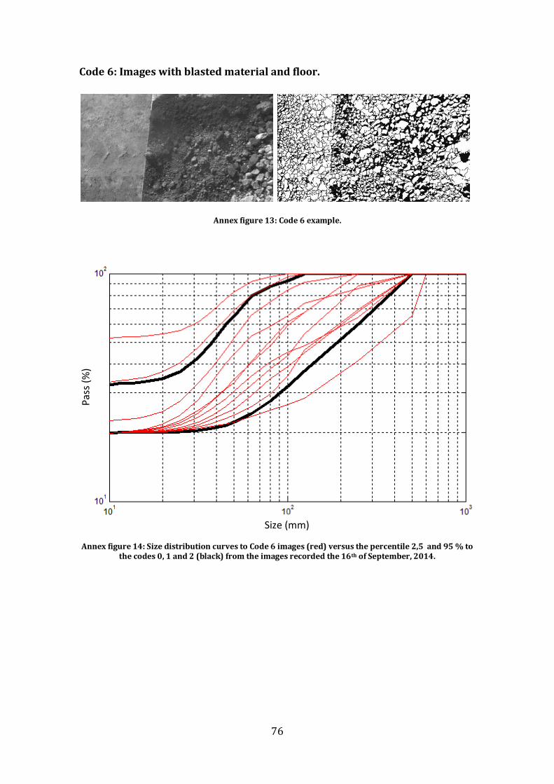
76

Code 6: Images with blasted material and floor.


Annex figure 14: Size distribution curves to Code 6 images (red) versus the percentile 2,5 and 95 % to

the codes 0, 1 and 2 (black) from the images recorded the 16th of September, 2014.

Pas

s (%

)

Size (mm)

77

Code 7: Images of empty trucks


Annex figure 16: Size distribution curves to Code 7 images (green) versus the percentile 2,5 and 95 %

to the codes 0, 1 and 2 (black) from the images recorded the 17th of September, 2014.

The curves corresponding to code 7 present a slope steeper than other codes.

Pas

s (%

)

Size (mm)

78

Code 8: Images of other kinds of vehicles


Annex figure 18: Size distribution curves to Code 8 images (red) versus the percentile 2,5 and 95 % to


Size (mm)

Pas

s (%

)

79

Code 9: Images with significant shadows.


Annex figure 20: Size distribution curves to Code 9 images (cyan) versus the percentile 2,5 and 95 % to


Code 9 images show a shape common to the Codes 0, 1 and 2, good quality images,

and are embraced by their 2,5 and 95 % percentiles. Thereby, the information

provided by images with shadow is also valid.

Pas

s (%

)

Size (mm)

80

ANNEX B

Resulting size fragmentation curves after filtering by the offline criterion the

images recorded grouped monthly.

Annex figure 21: September, 2014 size fragmentation curves.

81

Annex figure 22: October, 2014 size fragmentation curves.

Annex figure 23: November, 2014 size fragmentation curves.

82

Annex figure 24: December, 2014 size fragmentation curves.

Annex figure 25: March, 2014 size fragmentation curves.

83

Annex figure 26: April, 2014 size fragmentation curves.

Annex figure 27: May, 2014 size fragmentation curves.

84

ANNEX C

Analyzed Cobre la Cruces blasts summary.

Bla

sts

ID

Ben

ch

Vo

lum

e (m

3)

No

. B

ore

ho

les

No

. Ro

ws

Bu

rden

(m

)

Spac

ing

(m)

Hei

gh

t b

ench

(m

)

Dri

lled

m

eter

s

Spec

ific

ch

arge

(g

/m3)

EM

UN

EX

(k

g)

V420 -145 7850 105 14 4 4,5 4,5 472 593 4600

V805 -140 7800 140 4 4 4,62 3,8 133 535 4100

V806 -145 5800 88 11 4 4,62 3,9 31 594 3400

V812 -145 6902 84 7 4 4,62 4,5 54 585 4000

V815 -140 6978 88 8 4 4,62 4,7 52 665 4600

V816 -140 5123 70 7 4 4,62 4,95 50 688 3500

V823 -145 3895 55 5 4 4,62 3,8 42 649 2500

V824 -145 7562 88 8 4 4,62 4,65 51 693 5200

V825 -145 8300 112 8 4 4,5 4,2 59 609 5000

V828 -140 7750 84 7 4 4,62 4,94 59 690 5300

V829 -140 5600 87 3 4 4,5 4,5 130 545 3000

V835 -140 7200 129 3 4 4,5 4,65 200 509 3600

v841 -145 7100 91 7 4 4,62 4,12 54 570 4000

V845 -145 4420 88 8 4 4,6 3,73 41 552 2400

V851 -145 5000 84 4 4 4,62 3,95 83 528 2600

V854 -150 8660 104 8 4 4,5 4,5 58 722 6200

V860 -150 8100 120 4 4 4,5 4,75 142 576 4600

V862 -150 7043 91 7 4 4,5 4,3 56 659 4600

V867 -145 9767 114 9 4 4,5 4,9 559 702 6800

V873 -150 7500 106 8 4 4,5 3,98 422 607 4500

v934 -145 11000 133 10 4 4,5 4,9 652 606 6600

V938 -150 86000 1480 10 4 4,5 3,8 562 60 5100

V945 -165 8100 124 9 4 4,5 4,14 513 625 5000

V948 -150 8000 115 6 4 4,5 4 460 607 4800

V959 -155 12000 196 7 4 4,5 4,4 862 532 6300

V961 -115 10600 95 8 5 5 4,6 437 523 5500

V962 -115 10500 93 7 5 5 4,6 428 509 5300

V963 -155 6500 116 10 4 4,5 4 464 563 3600

85

Bla

sts

ID

Ben

ch

Vo

lum

e (m

3)

No

. B

ore

ho

les

No

. Ro

ws

Bu

rden

(m

)

Spac

ing

(m)

Hei

gh

t b

ench

(m

)

Dri

lled

m

eter

s

Spec

ific

ch

arge

(g

/m3)

EM

UN

EX

(k

g)

V964 -170 12000 153 8 4 4,5 4,5 688 614 7300

V968 -150 7000 90 6 4 4,5 4,9 441 606 4200

V973 -115 11000 137 11 5 5 4,5 616 560 6100

V978 -120 9400 109 11 4 4,5 4,8 523 750 7000

V980 -120 10400 131 8 4 4,5 5 655 678 7000

V985 -150 9500 143 10 4 4,5 4,5 644 629 5900

V987 -120 11300 126 9 4 4,5 5,1 643 766 8600

V990 -120 11800 120 6 4 4,5 5,5 660 708 8300

V991 -165 5000 99 7 4 4,5 3,2 317 509 2500

V992 -165 9000 144 7 4 4,5 4,3 619 619 5500

V995 -120 6600 79 9 4 4,5 4,7 371 748 4900

V997 -120 14670 163 6 4 4,5 5 815 653 9500

V1000 -170 6800 131 12 4 4,5 3,5 458 583 3900

V1002 -120 11700 131 7 4 4,5 5 655 749 8700

V1003 -125 12700 147 8 4 4,5 4,8 706 714 9000

V1004 -170 5500 104 5 4 4,5 4,3 447 665 3600

V1005 -120 9900 102 8 4 4,5 4,8 490 661 6500

V1007 -125 7317 123 3 4 4,5 4,75 584 611 4400

V1008 -175 9000 127 8 4 4,5 4,4 559 707 6300

V1009 -125 12900 145 10 4 4,5 5 725 765 9800

V1013 -125 9200 103 6 4 4,5 5 515 766 7000

V1014 -125 9000 134 7 4 4,5 4 536 763 6800

V1016 -175 8500 147 6 4 4,5 4 588 621 5200

escuela tÉcnica superior de ingenieros de...

Documents