
BIOKMOD. Aplicación a la modelización biocinética y farmacocinética
Actualizado: 2017‐01‐18
Guillermo Sánchez. (http://diarium.usal.es/guillermo)❦ Notas:
La presentación está elaborada con el programa BIOKMOD.
http://diarium.usal.es/guillermo/biokmod/
La mayoria de los ejemplos pueden reproducirse directamente en la web:
http://oed.usal.es/webMathematica/Biokmod/index.html
Santiago de Compostela. Enero 2017
http://diarium.usal.es/guillermo

¿Dónde queremos llegar?Mostrar como se puede utilizar BIOKMOD (BIOKinetic
MODelling) para: i) Modelizar proceso
biocinético/farmacocinético, ii) Obtener algunos de los
parámetros del modelo experimentalmente.
BIOKMOD está desarrollado usando el Wolfram Language
(requiere Mathematica 10 o superior). Esta disponible el
programa para descarga en:
http://diarium.usal.es/guillermo/biokmod/.
BiokmodWeb, es una versión que permite utilizar muchas
de las funcionalidades de BIOKMOD directamente desde un
navegador.
http://oed.usal.es/webMathematica/Biokmod/index.html
2 | BIOKMODenBIOSTACTNET2017.nb
http://diarium.usal.es/guillermo

Modelo bicompartimental simpleThe Figure represents an easy example of a two compartmental system of ingestion
and metabolism of a drug. It is supposed that the drug is taken orally flowing to the GI
tract (Compartment 1) , then it is absorbed into the blood (Compartment 2) and finally
eliminated.
Let x1(t) and x2(t), where t ≥ 0, is the mass of the drug in compartment 1 and 2, respec‐
tively. If it is assumed that rate of transference from each compartment i is propor‐
tional to the mass (or concentration) in this compartment. Then we can describe the
process as followⅆx1
ⅆt= { b(t) - drug distribution rate from 1 to 2} = b(t) - k12 x1
ⅆx2
ⅆt= {inflow rate (from 1) - outflow rate (elimination)} = k12 x1 - k20 x2
where k12 and k20 are the constants (>0) of proportionality from 1 to 2 and from 2 to
environment (elimination). This process is a simple case of first‐order kinetics. Both
ordinary differential equations (ODE) with appropriate initial conditions x1(0) and
x 2(0) constitute the compartmental metabolic model. In matrix‐vector format the
system of ordinary differential equation (SODE) model is
x1 ' (t)
x2 ' (t)=
-k12 0
k12 k20+
b(t)
0
BIOKMODenBIOSTACTNET2017.nb | 3
http://diarium.usal.es/guillermo
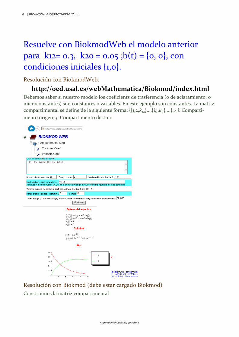
Resuelve con BiokmodWeb el modelo anterior
para k12= 0.3, k20 = 0.05 ;b(t) = {0, 0}, con
condiciones iniciales {1,0}.
Resolución con BiokmodWeb.
http://oed.usal.es/webMathematica/Biokmod/index.html Debemos saber si nuestro modelo los coeficients de trasferencia (o de aclaramiento, o
microconstantes) son constantes o variables. En este ejemplo son constantes. La matriz
compartimental se define de la siguiente forma: {{1,2,k12},...{i,j,kij},...}:> i: Comparti‐
mento origen; j: Compartimento destino.
❦
Resolución con Biokmod (debe estar cargado Biokmod)
Construimos la matriz compartimental
4 | BIOKMODenBIOSTACTNET2017.nb
http://diarium.usal.es/guillermo
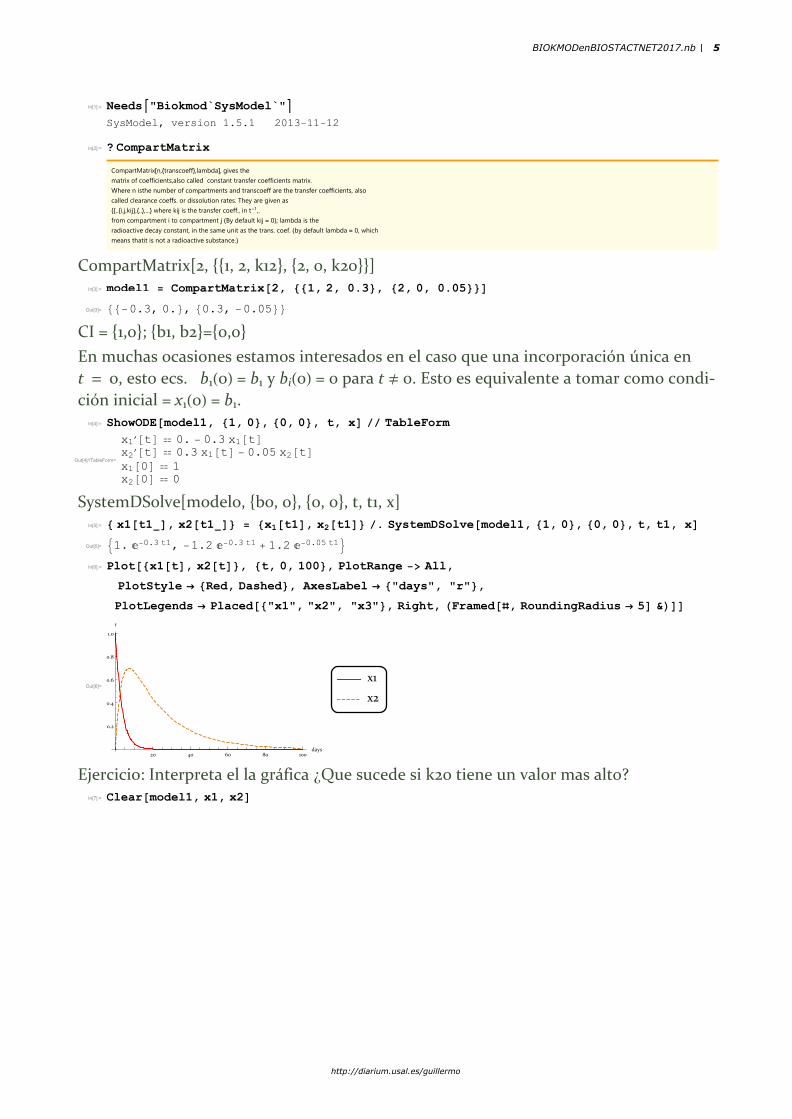
In[1]:= Needs"Biokmod`SysModel`"SysModel, version 1.5.1 2013-11-12
In[2]:= ? CompartMatrix
CompartMatrix[n,{transcoeff},lambda], gives thematrix of coefficients,also called constant transfer coefficients matrix.Where n isthe number of compartments and transcoeff are the transfer coefficients, alsocalled clearance coeffs. or dissolution rates. They are given as{{..{i,j,kij},{..},...} where kij is the transfer coeff., in t-1,.from compartment i to compartment j (By default kij = 0); lambda is theradioactive decay constant, in the same unit as the trans. coef. (by default lambda = 0, whichmeans thatit is not a radioactive substance.)
CompartMatrix[2, {{1, 2, k12}, {2, 0, k20}}]In[3]:= model1 = CompartMatrix[2, {{1, 2, 0.3}, {2, 0, 0.05}}]
Out[3]= {{-0.3, 0.}, {0.3, -0.05}}
CI = {1,0}; {b1, b2}={0,0}
En muchas ocasiones estamos interesados en el caso que una incorporación única en
t = 0, esto ecs. b1(0) = b1 y bi(0) = 0 para t ≠ 0. Esto es equivalente a tomar como condi‐
ción inicial = x1(0) = b1.In[4]:= ShowODE[model1, {1, 0}, {0, 0}, t, x] // TableForm
Out[4]//TableForm=
x1′[t] ⩵ 0. - 0.3 x1[t]x2′[t] ⩵ 0.3 x1[t] - 0.05 x2[t]x1[0] ⩵ 1x2[0] ⩵ 0
SystemDSolve[modelo, {b0, 0}, {0, 0}, t, t1, x]In[5]:= { x1[t1_], x2[t1_]} = {x1[t1], x2[t1]} /. SystemDSolve[model1, {1, 0}, {0, 0}, t, t1, x]
Out[5]= 1. ⅇ-0.3 t1, -1.2 ⅇ-0.3 t1 + 1.2 ⅇ-0.05 t1
In[6]:= Plot[{x1[t], x2[t]}, {t, 0, 100}, PlotRange -> All,
PlotStyle → {Red, Dashed}, AxesLabel → {"days", "r"},
PlotLegends → Placed[{"x1", "x2", "x3"}, Right, (Framed[#, RoundingRadius → 5] &)]]
Out[6]=
20 40 60 80 100days
0.2
0.4
0.6
0.8
1.0
r
x1
x2
Ejercicio: Interpreta el la gráfica ¿Que sucede si k20 tiene un valor mas alto?In[7]:= Clear[model1, x1, x2]
BIOKMODenBIOSTACTNET2017.nb | 5
http://diarium.usal.es/guillermo
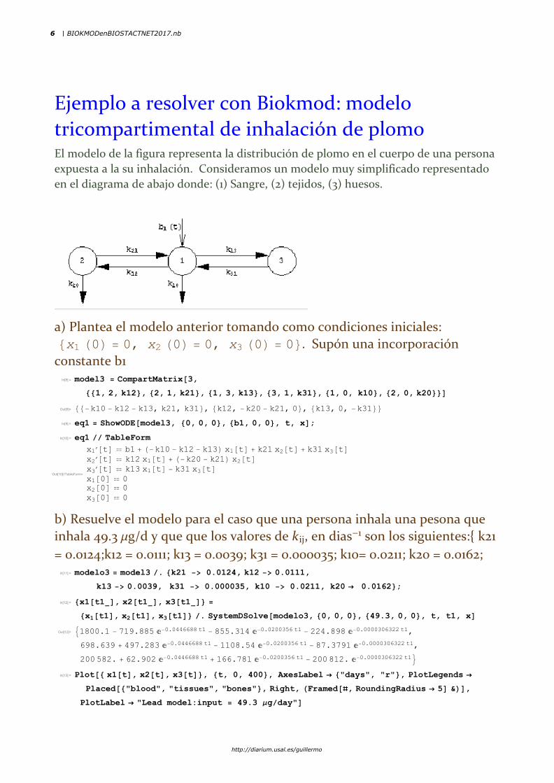
Ejemplo a resolver con Biokmod: modelo
tricompartimental de inhalación de plomoEl modelo de la figura representa la distribución de plomo en el cuerpo de una persona
expuesta a la su inhalación. Consideramos un modelo muy simplificado representado
en el diagrama de abajo donde: (1) Sangre, (2) tejidos, (3) huesos.
a) Plantea el modelo anterior tomando como condiciones iniciales:
{x1 (0) = 0, x2 (0) = 0, x3 (0) = 0}. Supón una incorporación
constante b1 In[8]:= model3 = CompartMatrix[3,
{{1, 2, k12}, {2, 1, k21}, {1, 3, k13}, {3, 1, k31}, {1, 0, k10}, {2, 0, k20}}]
Out[8]= {{-k10 - k12 - k13, k21, k31}, {k12, -k20 - k21, 0}, {k13, 0, -k31}}
In[9]:= eq1 = ShowODE[model3, {0, 0, 0}, {b1, 0, 0}, t, x];
In[10]:= eq1 // TableForm
Out[10]//TableForm=
x1′[t] ⩵ b1 + (-k10 - k12 - k13) x1[t] + k21 x2[t] + k31 x3[t]x2′[t] ⩵ k12 x1[t] + (-k20 - k21) x2[t]x3′[t] ⩵ k13 x1[t] - k31 x3[t]x1[0] ⩵ 0x2[0] ⩵ 0x3[0] ⩵ 0
b) Resuelve el modelo para el caso que una persona inhala una pesona que
inhala 49.3 μg/d y que que los valores de kij, en dias-1 son los siguientes:{ k21
= 0.0124;k12 = 0.0111; k13 = 0.0039; k31 = 0.000035; k10= 0.0211; k20 = 0.0162; In[11]:= modelo3 = model3 /. {k21 -> 0.0124, k12 -> 0.0111,
k13 -> 0.0039, k31 -> 0.000035, k10 -> 0.0211, k20 → 0.0162};
In[12]:= {x1[t1_], x2[t1_], x3[t1_]} =
{x1[t1], x2[t1], x3[t1]} /. SystemDSolve[modelo3, {0, 0, 0}, {49.3, 0, 0}, t, t1, x]
Out[12]= 1800.1 - 719.885 ⅇ-0.0446688 t1 - 855.314 ⅇ-0.0200356 t1 - 224.898 ⅇ-0.0000306322 t1,
698.639 + 497.283 ⅇ-0.0446688 t1 - 1108.54 ⅇ-0.0200356 t1 - 87.3791 ⅇ-0.0000306322 t1,
200 582. + 62.902 ⅇ-0.0446688 t1 + 166.781 ⅇ-0.0200356 t1 - 200812. ⅇ-0.0000306322 t1
In[13]:= Plot[{ x1[t], x2[t], x3[t]}, {t, 0, 400}, AxesLabel → {"days", "r"}, PlotLegends →
Placed[{"blood", "tissues", "bones"}, Right, (Framed[#, RoundingRadius → 5] &)],
PlotLabel → "Lead model:input = 49.3 μg/day"]
6 | BIOKMODenBIOSTACTNET2017.nb
http://diarium.usal.es/guillermo

Out[13]=
100 200 300 400days
500
1000
1500
2000
rLead model:input = 49.3 μg/day
blood
tissues
bones
c) Interpreta la salida gráficaIn[14]:= Clear[b1, k, a, x1, x2, x3, eq1, model3, modelo3];
BIOKMODenBIOSTACTNET2017.nb | 7
http://diarium.usal.es/guillermo
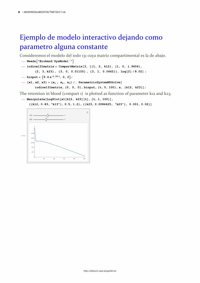
Ejemplo de modelo interactivo dejando como
parametro alguna constanteConsideremos el modelo del iodo 131 cuya matriz compartimental es la de abajo.
In[15]:= Needs"Biokmod`SysModel`"
In[16]:= iodine131matrix = CompartMatrix[3, {{1, 2, k12}, {1, 0, 1.9404},
{2, 3, k23} , {3, 0, 0.01155} , {3, 1, 0.0462}}, Log[2] / 8.02] ;
In[17]:= binput = 9.4 ⅇ-0.93 t, 0, 0;
In[18]:= {x1, x2, x3} = {x1 , x2, x3} /. ParametricSystemNDSolve[
iodine131matrix, {0, 0, 0}, binput, {t, 0, 100}, x, {k12, k23}];
The retention in blood (compart 1) is plotted as function of parameter k12 and k23.In[19]:= Manipulate[LogPlot[x1[k12, k23][t], {t, 1, 100}],
{{k12, 0.83, "k13"}, 0.5, 1.2}, {{k23, 0.0086625, "k23"}, 0.001, 0.02}]
Out[19]=
k13
k23
20 40 60 80 100
10-5
10-4
0.001
0.010
0.100
1
8 | BIOKMODenBIOSTACTNET2017.nb
http://diarium.usal.es/guillermo
Regresión no lineal. Ajuste de modelos In[20]:= Clear"Global`*"
(Solo disponible en Biokmod)
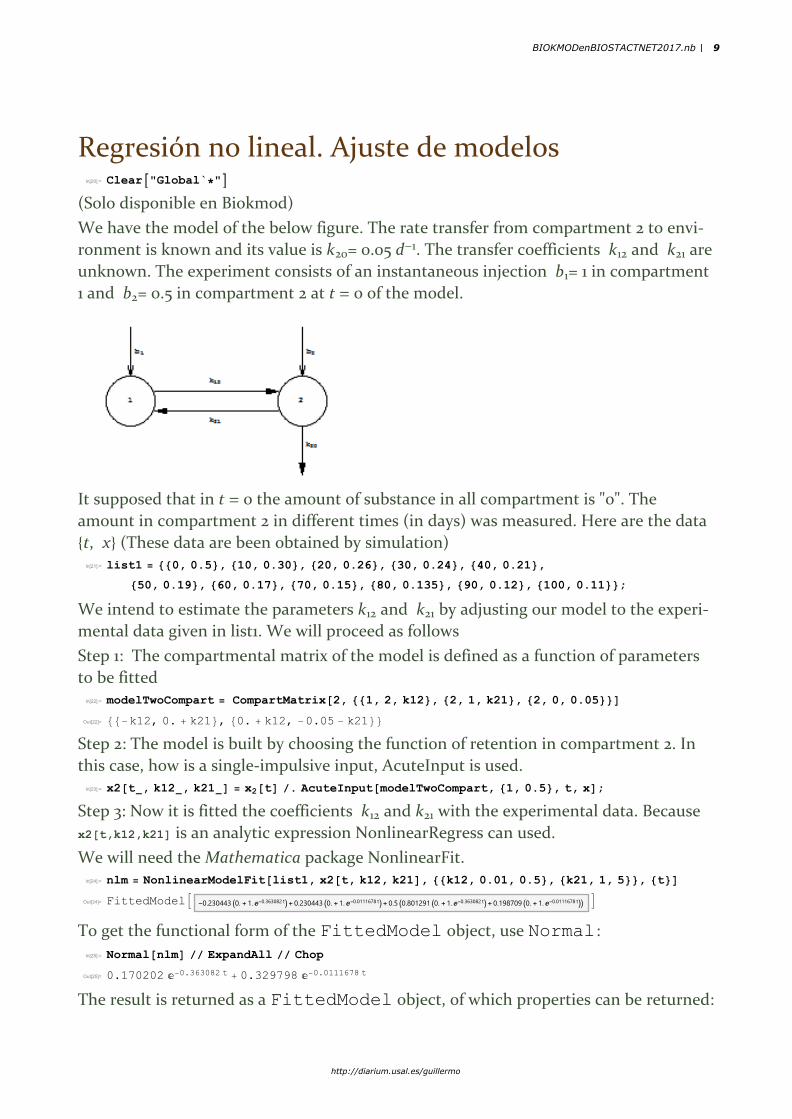
We have the model of the below figure. The rate transfer from compartment 2 to envi‐
ronment is known and its value is k20= 0.05 d-1. The transfer coefficients k12 and k21 are
unknown. The experiment consists of an instantaneous injection b1= 1 in compartment
1 and b2= 0.5 in compartment 2 at t = 0 of the model.
It supposed that in t = 0 the amount of substance in all compartment is "0". The
amount in compartment 2 in different times (in days) was measured. Here are the data
{t, x} (These data are been obtained by simulation)In[21]:= list1 = {{0, 0.5}, {10, 0.30}, {20, 0.26}, {30, 0.24}, {40, 0.21},
{50, 0.19}, {60, 0.17}, {70, 0.15}, {80, 0.135}, {90, 0.12}, {100, 0.11}};
We intend to estimate the parameters k12 and k21 by adjusting our model to the experi‐
mental data given in list1. We will proceed as follows
Step 1: The compartmental matrix of the model is defined as a function of parameters
to be fittedIn[22]:= modelTwoCompart = CompartMatrix[2, {{1, 2, k12}, {2, 1, k21}, {2, 0, 0.05}}]
Out[22]= {{-k12, 0. + k21}, {0. + k12, -0.05 - k21}}
Step 2: The model is built by choosing the function of retention in compartment 2. In
this case, how is a single‐impulsive input, AcuteInput is used.In[23]:= x2[t_, k12_, k21_] = x2[t] /. AcuteInput[modelTwoCompart, {1, 0.5}, t, x];
Step 3: Now it is fitted the coefficients k12 and k21 with the experimental data. Because
x2[t,k12,k21] is an analytic expression NonlinearRegress can used.
We will need the Mathematica package NonlinearFit. In[24]:= nlm = NonlinearModelFit[list1, x2[t, k12, k21], {{k12, 0.01, 0.5}, {k21, 1, 5}}, {t}]
Out[24]= FittedModel -0.230443 0. + 1. ⅇ-0.363082 t + 0.230443 0. + 1. ⅇ-0.0111678 t + 0.5 0.801291 0. + 1. ⅇ-0.363082 t + 0.198709 0. + 1. ⅇ-0.0111678 t
To get the functional form of the FittedModel object, use Normal :
In[25]:= Normal[nlm] // ExpandAll // Chop
Out[25]= 0.170202 ⅇ-0.363082 t + 0.329798 ⅇ-0.0111678 t
The result is returned as a FittedModel object, of which properties can be returned:
BIOKMODenBIOSTACTNET2017.nb | 9
http://diarium.usal.es/guillermo

In[26]:= nlm["Properties"]
Out[26]= {AdjustedRSquared, AIC, AICc, ANOVATable, ANOVATableDegreesOfFreedom,
ANOVATableEntries, ANOVATableMeanSquares, ANOVATableSumsOfSquares,
BestFit, BestFitParameters, BIC, CorrelationMatrix, CovarianceMatrix,
CurvatureConfidenceRegion, Data, EstimatedVariance, FitCurvatureTable,
FitCurvatureTableEntries, FitResiduals, Function, HatDiagonal,
MaxIntrinsicCurvature, MaxParameterEffectsCurvature, MeanPredictionBands,
MeanPredictionConfidenceIntervals, MeanPredictionConfidenceIntervalTable,
MeanPredictionConfidenceIntervalTableEntries, MeanPredictionErrors,
ParameterBias, ParameterConfidenceIntervals, ParameterConfidenceIntervalTable,
ParameterConfidenceIntervalTableEntries, ParameterConfidenceRegion,
ParameterErrors, ParameterPValues, ParameterTable, ParameterTableEntries,
ParameterTStatistics, PredictedResponse, Properties, Response,
RSquared, SingleDeletionVariances, SinglePredictionBands,
SinglePredictionConfidenceIntervals, SinglePredictionConfidenceIntervalTable,
SinglePredictionConfidenceIntervalTableEntries,
SinglePredictionErrors, StandardizedResiduals, StudentizedResiduals}
In[27]:= nlm[{"ParameterTable", "ANOVATable"}]
Out[27]= Estimate Standard Error t- Statistic P- Value
k12 0.0810964 0.0122265 6.63285 0.0000955992k21 0.243154 0.0422701 5.75238 0.000275471
,DF SS MS
Model 2 0.641483 0.320741Error 9 0.0000420101 4.66779 × 10⁻⁶Uncorrected Total 11 0.641525Corrected Total 10 0.124414
Here the fitted function and the experimental data are shown:In[28]:= Plot[x2[t, 0.081, 0.2431], {t, 0, 100},
Epilog → {Hue[0], PointSize[0.02], Map[Point, list1]}]
Out[28]=
20 40 60 80 100
0.2
0.3
0.4
0.5
In[29]:= Clear"Global`*"
Se pueden consultar mas ejemplos, incluido modelos multirespuesta en la ayuda de
BIOKMOD
10 | BIOKMODenBIOSTACTNET2017.nb
http://diarium.usal.es/guillermo

Mas lejos: Modelos no lineales (Ver ejemplos en la
ayuda del programa).
Here is solved 2 D Fick' s law of diffusion from the boundaries of a circleIn[30]:= Ω = ImplicitRegionx2 + y2 ≤ 10, {{x, -5, 5}, {y, -5, 5}};
eq1 = D[u[x, y, t], t] ⩵ 0.0000072 * (D[u[x, y, t], x, x] + D[u[x, y, t], y, y]) - 1.2;
sol = NDSolveeq1, DirichletConditionu[x, y, t] ⩵ 100, x2 + y2 ⩵ 10,
u[x, 0, t] ⩵ 10, u[0, y, t] ⩵ 10, u[x, y, 0] ⩵ 10, u, {t, 0, 10}, {x, y} ∈ Ω;
Animate[ContourPlot[u[x, y, t] /. sol,
{x, y} ∈ Ω, PlotRange → {0, 10}, ClippingStyle → Automatic,
ColorFunction → "DarkRainbow", PlotLegends → Automatic], {t, 0, 100}]
Out[34]=
BIOKMODenBIOSTACTNET2017.nb | 11
http://diarium.usal.es/guillermo

Diseño óptimo de experimentos: (Ver ejemplos en
la ayuda del programa y referencias al final)In[35]:= Quit[]
BIOMODWEB:> Statistic:>Optimal Design
In[14]:= Quit[]
The same computation can be made directely using the package functions OptdesIn[1]:= Needs"Biokmod`Optdesign`"
Optdesign, 1.0 2007-04-09
In[2]:= Optdes inp ⅇ- 2.0 t- 0.09 p + ⅇ- 0.001 t- 0.2 p, t, {{inp, 100}, {p, 5}} , 0.5, 1, 2, 1
Out[2]= {0.055815, {t0 → 0.5, t1 → 3.95733}}
BIOMOD. Step by stepIn[3]:= Needs"Biokmod`SysModel`"
SysModel, version 1.5.1 2013-11-12
Let's consider the iodine biokinetic model before describe. k10= 1.9404, k30= 0.01155,
k31= 0.0462. We will suppose that k12 and k23 are unknown (ICRP gives for a standard
man k12= 0.8316, k23 = 0.0086625)
We will refer to iodine 131 which has a radioactive half‐life of 8.02 days, this meaning
that radioactive decay constant λ = ln 2/8.02 day-1. Then the compartmental matrix is:In[4]:= iodine131matrix = CompartMatrix[3, {{1, 2, k12}, {1, 0, 1.9404},
{2, 3, k23} , {3, 0, 0.01155} , {3, 1, 0.0462}}, Log[2] / 8.02] // Chop
Out[4]= {{-2.02683 - k12, 0, 0.0462}, {k12, -0.0864273 - k23, 0}, {0, k23, -0.144177}}
A input b1= 27.13 ⅇ-24.08 t + 27.13 ⅇ-2.86 t - 0.02 ⅇ-0.147 t + 0.0194 ⅇ-0.093 t
happens in compartment 1, and b=0 in the others (This kind of input happens in real
situations when there is an input from the GIT (Gastro Intestinal) to the blood, for
instance if the iodine is intaken by orally.. Then:In[5]:= binput = -27.13 ⅇ-24.08 t + 27.13 ⅇ-2.86 t - 0.020 ⅇ-0.147 t + 0.0194 ⅇ-0.093 t, 0, 0;
12 | BIOKMODenBIOSTACTNET2017.nb
http://diarium.usal.es/guillermo
The initial condition are { 0, 0, 0}. In[6]:= ic = {0, 0, 0};
The numerical solution of the system as function of the parametes {k12, k23} can be
obtained using the package function ParametricSystemNDSolve ( the Mathematica ‐9
or later‐ function ParametricNDSolve is used )
In[7]:= {x1, x2, x3} = {x1 , x2, x3} /.
ParametricSystemNDSolve[iodine131matrix, ic, binput, {t, 0, 100}, x, {k12, k23}];
We are intesting in estimated k12 and k23 taken sample of the iodine in the compart‐
ment 1. The problem consist on decide by Optimum Design Experiment (ODE) the best
moment {t0, t1, ...} to taken these samples.
We need the derivatives in compartment 1, that is ∇(x1(t), {k12, k23}) In[8]:= fa[a1_?NumberQ, b_?NumberQ, t_?NumberQ] := D[x1[a, b], a][t] /. a → a1
In[9]:= fb[a_?NumberQ, b1_?NumberQ, t_?NumberQ] := D[x1[a, b], b][t] /. b → b1
In[10]:= X1[a_, b_, ti_] := { fa[a, b, ti], fb[a, b, ti]}
A typical election for compute the covariance matrix is assumed that that the relation‐
ship between samples decays exponentially with increasing time‐distance between
them, that is Γ = {lij} with lij= exp {ρ|tj -tj|}.For computational purpose we have found
more appropriate to use the distance di = ti - ti-1, instead of ti, then ti= ∑i di being
d0 = t0 . That is for a two points design . We suppose a 3‐points design.
Γ where In[11]:= Γ = 1, ⅇ-ρ d1, ⅇ-ρ (d1+d2), ⅇ-ρ d1, 1, ⅇ-ρ d2, ⅇ-ρ (d1+d2), ⅇ-ρ d2, 1;
Now it is computed the covariance matrix Σ = σ2 ΓIn[12]:= Σ = σ2 * Γ;
We assume In[13]:= ρ = 1; σ = 1;
We will also need give the initial values of β the standard deviation of the measures.
We also assumed k12= 0.80, k23=0.0078.Then we can obtain the information matrix
M = XT Σ-1 X
m := X . Inverse[Σ]. Transpose[X];In[14]:= m1[ti_] :=
Transpose[Map[X1[0.80, 0.0078, #] &, ti] ]. Inverse[Σ].Map[X1[0.80, 0.0078, #] &, ti]
8.‐ Finally the determinant of the information matrix is maximized as function of d0,
d1 and d2. We constrain the d values to a maximun of t=50 becouse to longer time the
concentration will be very low (lower than the detection limit)In[15]:= obj[d0_?NumericQ, d1_?NumericQ, d2_?NumericQ] := Det[m1[{d0, d1 + d0, d0 + d1 + d2}]]
In[16]:= sol1 = NMaximize[
{obj[d0, d1, d2], 0 < d0 < 50, 0.02 < d1 < 50, 0.02 < d2 < 50}, {d0, d1, d2}] // Quiet
Out[16]= {0.0160626, {d0 → 0.748664, d1 → 7.23753, d2 → 3.66114}}
Then the observation should be taken at: t0, t1 t2 (in days starting in t=0)
BIOKMODenBIOSTACTNET2017.nb | 13
http://diarium.usal.es/guillermo

In[17]:= { d0, d1 + d0, d0 + d1 + d2} /. sol1[[2]]
Out[17]= {0.748664, 7.98619, 11.6473}
14 | BIOKMODenBIOSTACTNET2017.nb
http://diarium.usal.es/guillermo
Material adicional:
http://diarium.usal.es/guillermohttp://diarium.usal.es/guillermo/biokmod/
Mathematica Beyond Mathematics: The Wolfram Language in the Real World
(March 15, 2017. Chapman and Hall/CRC
https://www.crcpress.com/Mathematica‐Beyond‐Mathematics‐The‐Wolfram‐Lan‐
guage‐in‐the‐Real‐World/Sanchez‐Leon/p/book/9781498796293
Mathematica más allá de las matemáticas. 2ª Edición (marzo 2015, actualizado a Mathe‐
matica 10). Disponible en GoogleBooks y Playstore.
Tutoriales y presentaciones en youtube: http://diarium.usal.es/guillermo/mathemat‐
ica/
Bibliografia: http://diarium.usal.es/guillermo/publicaciones/especializadas/
Sobre Biokmod, bioensayos y modelización compartimental
Sánchez G; “Fitting bioassay data and performing uncertainty analysis with BIOKMOD”
Health Physics.. 92(1) :64‐72. 2007. ISSN/ISBN: 0017‐9078
Sánchez G; Biokmod: A Mathematica toolbox for modeling Biokinetic Systems”.
Mathematica in Education and Research: 10 (2) 2005. ISSN/ISBN: 1096‐3324
Lopez‐Fidalgo J; Sánchez G; Statistical Criteria to Establish Bioassay Programs. Health
Physics.. 89 (4). 2005. ISSN/ISBN: 0017‐9078
Sánchez G; Lopez‐Fidalgo J “Mathematical Techniques for Solving Analytically Large
Compartmental Systems” Health Physics..: 85 (2): 2003. ISSN/ISBN: 0017‐9078
Sobre diseño óptimo:
Juan M. Rodríguez‐Díaz;Guillermo Sánchez‐León:”Design optimality for models defined
by a system of ordinary differential equations” Biometrical Journal 56 (5), pag 886–900,
September 2014
G. Sánchez; J. M. Rodríguez‐Díaz . Optimal design and mathematical model applied to
establish bioassay programs”: Radiation Protection Dosimetry. doi:10.1093/rpd/ncl499.
2007. ISSN/ISBN: ISSN 1742‐3406
Lopez‐Fidalgo J Rodriıguez‐Díaz J.M.,Sánchez G; G., Santos‐Martín M.T. Optimal designs
for compartmental models with correlated observations” Journal of Applied Statistic. 32,
2006 ISSN/ISBN: 0266‐4763
BIOKMODenBIOSTACTNET2017.nb | 15
http://diarium.usal.es/guillermo


