DOCUMENTS DE TREBALL

DE LA FACULTAT D’ECONOMIA I EMPRESA

Col.lecció d’Economia

E12/282

Monge assignment games

F. Javier Martínez de Albéniz

Carles Rafels F. Javier Martínez de Albéniz Dep. de Matemàtica Econòmica, Financera i Actuarial. Universitat de Barcelona Av. Diagonal 690, 08034 Barcelona, Spain. javier.martinezdealbeniz@ub.edu Carles Rafels Dep. de Matemàtica Econòmica, Financera i Actuarial. Universitat de Barcelona Av. Diagonal 690, 08034 Barcelona, Spain. crafels@ub.edu The authors acknowledge the support from research grants ECO2011-22765/ECON (Ministerio de Ciencia e Innovación and FEDER) and 2009SGR960 (Generalitat de Catalunya).

AbstractAn assignment game is defined by a matrix A, where each row represents

a buyer and each column a seller. If buyer i is matched with seller j, themarket produces aij units of utility. We study Monge assignment games,that is bilateral cooperative assignment games where the assignment matrixsatisfies the Monge property. These matrices can be characterized by thefact that in any submatrix of 2 × 2 an optimal matching is placed in itsmain diagonal. For square markets, we describe their cores by using only thecentral tridiagonal band of the elements of the matrix. We obtain a closedformula for the buyers-optimal and the sellers-optimal core allocations. Non-square markets are analyzed also by reducing them to appropriate squarematrices.

Key words: assignment game, core, Monge matrix, buyers-optimal coreallocation, sellers-optimal core allocation

JEL Code: C71

ResumenUn juego de asignacion se define por una matriz A, donde cada fila re-

presenta un comprador y cada columna un vendedor. Si el comprador ise empareja a un vendedor j, el mercado produce aij unidades de utilidad.Estudiamos los juegos de asignacion de Monge, es decir, aquellos juegos bila-terales de asignacion en los cuales la matriz satisface la propiedad de Monge.Estas matrices pueden caracterizarse por el hecho de que en cualquier sub-matriz 2×2 un emparejamiento optimo esta situado en la diagonal principal.Para mercados cuadrados, describimos sus nucleos utilizando solo la partecentral tridiagonal de elementos de la matriz. Obtenemos una formula ce-rrada para el reparto optimo de los compradores dentro del nucleo y para elreparto optimo de los vendedores dentro del nucleo. Analizamos tambien losmercados no cuadrados reduciendolos a matrices cuadradas apropiadas.

Palabras clave: juego de asignacion, nucleo, matriz Monge, repartooptimo para los vendedores, reparto optimo para los compradores

Codigo JEL: C71

2

1. Introduction

The optimal (linear sum) assignment problem is that of finding an optimalmatching, given a matrix that collects the potential profit of each pair ofagents. Some examples are the placement of workers to jobs, of studentsto colleges, of physicians to hospitals or the pairing of men and women inmarriage. Once an optimal matching has been found, one question arises:how to share the output among the partners. This question, that has beenmainly addressed in the field of game theory, was first considered in Shapleyand Shubik (1972). They associate to each assignment problem a cooperativegame, or game in coalitional form.

In the assignment game, each coalition of agents must consider the max-imum profit they could attain by themselves as the worth of this coalition.The most relevant solution concept in cooperative games is the core. Thecore of a game consists of those allocations of the optimal profit (the worthof the grand coalition) such that no subcoalition can improve upon. Thus,if we agree to share the profit of cooperation by means of a core allocation,no coalition has incentives to depart from the grand coalition and act onits own. Shapley and Shubik prove that the core of the assignment gameis a nonempty polyhedral convex set and it coincides with the set of solu-tions of the dual linear program related to the linear sum optimal assignmentproblem.

In this paper we study the assignment games, called Monge assignmentgames, where the matrix satisfies what is called the Monge property. Roughlyspeaking, the (inverse) Monge property is described by the fact that each 2×2submatrix has an optimal matching in the main diagonal. This property canalso be identified as the supermodularity of the matrix, interpreted as afunction on the product of the set of indices with the usual order.

Monge matrices have been used in different fields in Operations Research,such as combinatorial optimization (see Burkard et al., 1996 or Burkard,2007), coalitional game theory (see Okamoto, 2004), algorithmic issues (seeBein et al., 2005), or statistics (see Hou and Prekopa, 2007).

For square Monge assignment games, the central tridiagonal band of thematrix, that is the main diagonal, the sub-diagonal and the super-diagonal,is sufficient to determine the core. As a result, and differently to the generalcase, not all inequalities are necessary to describe the core explicitly, andin this case the buyer-seller exact representative of the matrix (Nunez andRafels, 2002b) can be computed by a closed formula. Two important points

3

of the core, the buyers-optimal and the sellers-optimal core allocations, arecomputed and related to specific 2×2 submarkets. The last part of the paperis devoted to the non-square Monge assignment games.

The paper is organized as follows. In Section 2 we describe the assignmentgame and the results on it we will need later. In Section 3, the Mongeassignment markets are defined. We describe the core of the square Mongeassignment game, and give a way to compute easily its buyer-seller exactrepresentative matrix and in Section 4 we compute the buyers-optimal andthe sellers-optimal core allocations and give a formula to obtain them. Weconclude in Section 5 by analyzing non-square Monge assignment markets,their core and the buyers-optimal and sellers-optimal core allocations.

2. Preliminaries on the assignment game

A bilateral assignment market (M,M ′, A) is defined by a nonempty finiteset of agents, usually named buyers M , a nonempty finite set of anothertype of agents, usually named sellers M ′ and a nonnegative matrix A =(aij)(i,j)∈M×M ′ . Entry aij represents the profit obtained by the mixed-pair

(i, j) ∈M ×M ′ if they trade. Let us assume there are |M | = m buyers and|M ′| = m′ sellers. If m = m′, the assignment market is said to be square.Let us denote by M+

m×m′ the set of nonnegative matrices with m rows andm′ columns.

A matching µ ⊆M ×M ′ between M and M ′ is a bijection from M0 ⊆Mto M ′

0 ⊆ M ′, such that |M0| = |M ′0| = min {|M | , |M ′|}. We write (i, j) ∈ µ

as well as j = µ (i) or i = µ−1 (j) . The set of all matchings is denoted byM (M,M ′). A buyer i ∈ M is unmatched by µ if there is no j ∈ M ′ suchthat (i, j) ∈ µ. Similarly, j ∈ M ′ is unmatched by µ if there is no i ∈ Msuch that (i, j) ∈ µ.

A matching µ ∈M (M,M ′) is optimal for the assignment market (M,M ′, A)if for all µ′ ∈ M (M,M ′) we have

∑(i,j)∈µ aij ≥

∑(i,j)∈µ′ aij, and we denote

the set of optimal matchings by M∗A (M,M ′).

Shapley and Shubik (1972) associate to any assignment market a gamein coalitional form (assignment game) with player set N = M ∪ M ′ andcharacteristic function wA defined by A in the following way: for S ⊆M and

T ⊆ M ′, wA (S ∪ T ) = max{∑

(i,j)∈µ aij | µ ∈M (S, T )}

, where M(S, T ) is

the set of matchings from S to T and wA(S ∪ T ) = 0 if M(S, T ) = ∅.

4

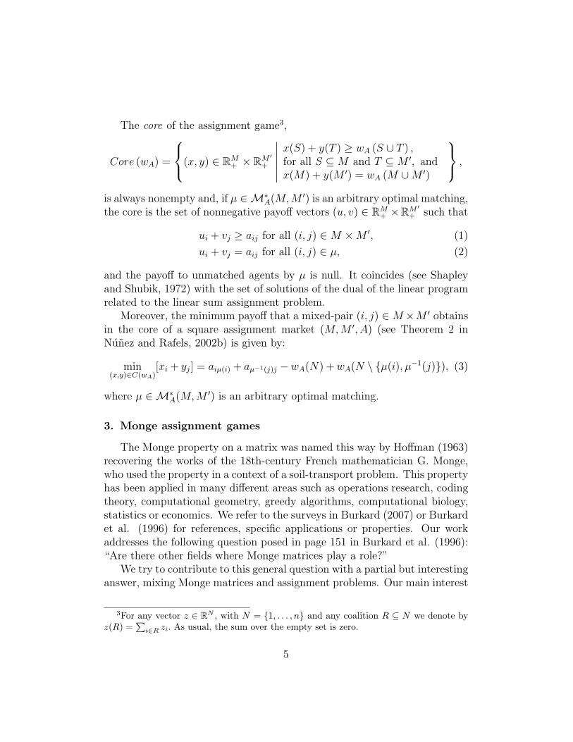
The core of the assignment game3,

Core (wA) =

(x, y) ∈ RM+ × RM′

+

∣∣∣∣∣∣x(S) + y(T ) ≥ wA (S ∪ T ) ,for all S ⊆M and T ⊆M ′, andx(M) + y(M ′) = wA (M ∪M ′)

,

is always nonempty and, if µ ∈M∗A(M,M ′) is an arbitrary optimal matching,

the core is the set of nonnegative payoff vectors (u, v) ∈ RM+ ×RM′

+ such that

ui + vj ≥ aij for all (i, j) ∈M ×M ′, (1)

ui + vj = aij for all (i, j) ∈ µ, (2)

and the payoff to unmatched agents by µ is null. It coincides (see Shapleyand Shubik, 1972) with the set of solutions of the dual of the linear programrelated to the linear sum assignment problem.

Moreover, the minimum payoff that a mixed-pair (i, j) ∈M×M ′ obtainsin the core of a square assignment market (M,M ′, A) (see Theorem 2 inNunez and Rafels, 2002b) is given by:

min(x,y)∈C(wA)

[xi + yj] = aiµ(i) + aµ−1(j)j −wA(N) +wA(N \ {µ(i), µ−1(j)}), (3)

where µ ∈M∗A(M,M ′) is an arbitrary optimal matching.

3. Monge assignment games

The Monge property on a matrix was named this way by Hoffman (1963)recovering the works of the 18th-century French mathematician G. Monge,who used the property in a context of a soil-transport problem. This propertyhas been applied in many different areas such as operations research, codingtheory, computational geometry, greedy algorithms, computational biology,statistics or economics. We refer to the surveys in Burkard (2007) or Burkardet al. (1996) for references, specific applications or properties. Our workaddresses the following question posed in page 151 in Burkard et al. (1996):“Are there other fields where Monge matrices play a role?”

We try to contribute to this general question with a partial but interestinganswer, mixing Monge matrices and assignment problems. Our main interest

3For any vector z ∈ RN , with N = {1, . . . , n} and any coalition R ⊆ N we denote byz(R) =

∑i∈R zi. As usual, the sum over the empty set is zero.

5

is to describe the core and the two sectors-optimal core allocations in aneasy and practical way, when dealing with Monge assignment cooperativegames. Roughly speaking, our results agree with the “flavor” that addingthe Monge conditions to the assignment game simplifies a lot the analysis ofthe aforementioned solutions. Finally, this class of assignment markets havean important economic meaning, especially when we deal with agents thatcan be ordered according some trait such as age, education, income, etc. (seeBecker, 1973).

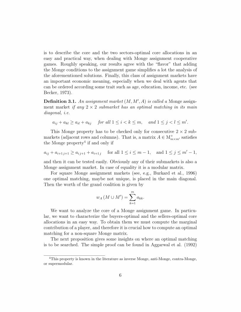
Definition 3.1. An assignment market (M,M ′, A) is called a Monge assign-ment market if any 2 × 2 submarket has an optimal matching in its maindiagonal, i.e.

aij + akl ≥ ail + akj for all 1 ≤ i < k ≤ m, and 1 ≤ j < l ≤ m′.

This Monge property has to be checked only for consecutive 2 × 2 sub-markets (adjacent rows and columns). That is, a matrix A ∈ M+

m×m′ satisfiesthe Monge property4 if and only if

aij + ai+1 j+1 ≥ ai j+1 + ai+1 j for all 1 ≤ i ≤ m− 1, and 1 ≤ j ≤ m′ − 1,

and then it can be tested easily. Obviously any of their submarkets is also aMonge assignment market. In case of equality it is a modular matrix.

For square Monge assignment markets (see, e.g., Burkard et al., 1996)one optimal matching, maybe not unique, is placed in the main diagonal.Then the worth of the grand coalition is given by

wA (M ∪M ′) =m∑k=1

akk.

We want to analyze the core of a Monge assignment game. In particu-lar, we want to characterize the buyers-optimal and the sellers-optimal coreallocations in an easy way. To obtain them we must compute the marginalcontribution of a player, and therefore it is crucial how to compute an optimalmatching for a non-square Monge matrix.

The next proposition gives some insights on where an optimal matchingis to be searched. The simple proof can be found in Aggarwal et al. (1992)

4This property is known in the literature as inverse Monge, anti-Monge, contra-Monge,or supermodular.

6

or in Lin (1992). It generalizes the fact that the main diagonal is an optimalmatching if we deal with square Monge assignment markets.

Proposition 3.1. For any Monge assignment market (M,M ′, A), with |M | ≤|M ′|, at least one optimal matching µ ∈M∗

A(M,M ′) is monotone, i.e.

for all i1, i2 ∈M, with i1 < i2, then µ(i1) < µ(i2).

Monotone matchings can be seen as generalized main diagonal matchings,since they coincide with the matching given by the main diagonal entriesof the square submarkets of maximal order. When the Monge assignmentmarket is square, there is only one monotone matching, which is placed inthe main diagonal. Therefore, if necessary, to distinguish the agents fromthe two sides of the market we will denote by k′ ∈ M ′ the partner of playerk ∈M by this optimal matching.

Now we are in position to give an easy description of the core of a squareMonge assignment game.

Theorem 3.1. Let (M,M ′, A) be a square Monge assignment market. Then(u, v) ∈ RM+ × RM

′+ belongs to the core of the market, C(wA), if and only if

ui + vi = aii for i = 1, 2, . . . ,m, (4)

ui + vi+1 ≥ ai i+1 for i = 1, 2, . . . ,m− 1, (5)

ui+1 + vi ≥ ai+1 i for i = 1, 2, . . . ,m− 1. (6)

Proof. The ’only if’ part is obvious by the definition of the core of an assign-ment game, see (1) and (2), and the fact that one optimal matching is placedin the main diagonal.

Now to prove the ’if’ part, consider for i + 1 < j, the square submarketformed by {i, i+ 1, . . . , j − 1}×{i′ + 1, . . . , j′} . One optimal matching in thesquare Monge submarket is placed in the main diagonal of the submatrix,that is, µ = {(i, i+ 1), (i+ 1, i+ 2), . . . , (j − 1, j)} , and then:

j−1∑k=i

ak k+1 ≥ aij +

j−1∑k=i+1

akk.

Now, considering (4) and (5), we obtain

ui + vj =

j−1∑k=i

uk +

j∑k=i+1

vk −j−1∑k=i+1

akk ≥j−1∑k=i

ak k+1 −j−1∑k=i+1

akk ≥ aij.

7

If j + 1 < i, just take the submarket {j + 1, . . . , i} × {j′, . . . , (i− 1)′} , andrepeat a similar argument.

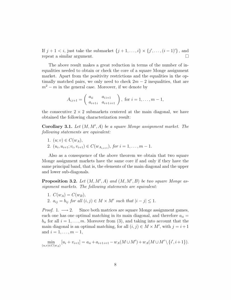
The above result makes a great reduction in terms of the number of in-equalities needed to obtain or check the core of a square Monge assignmentmarket. Apart from the positivity restrictions and the equalities in the op-timally matched pairs, we only need to check 2m − 2 inequalities, that arem2 −m in the general case. Moreover, if we denote by

Ai,i+1 =

(aii ai i+1

ai+1 i ai+1 i+1

), for i = 1, . . . ,m− 1,

the consecutive 2 × 2 submarkets centered at the main diagonal, we haveobtained the following characterization result:

Corollary 3.1. Let (M,M ′, A) be a square Monge assignment market. Thefollowing statements are equivalent:

1. (u; v) ∈ C(wA),

2. (ui, ui+1; vi, vi+1) ∈ C(wAi,i+1), for i = 1, . . . ,m− 1.

Also as a consequence of the above theorem we obtain that two squareMonge assignment markets have the same core if and only if they have thesame principal band, that is, the elements of the main diagonal and the upperand lower sub-diagonals.

Proposition 3.2. Let (M,M ′, A) and (M,M ′, B) be two square Monge as-signment markets. The following statements are equivalent:

1. C(wA) = C(wB),

2. aij = bij for all (i, j) ∈M ×M ′ such that |i− j| ≤ 1.

Proof. 1. −→ 2. Since both matrices are square Monge assignment games,each one has one optimal matching in its main diagonal, and therefore aii =bii for all i = 1, . . . ,m. Moreover from (3), and taking into account that themain diagonal is an optimal matching, for all (i, j) ∈M ×M ′, with j = i+ 1and i = 1, . . . ,m− 1,

min(u,v)∈C(wA)

[ui + vi+1] = aii+ai+1 i+1−wA(M ∪M ′)+wA(M ∪M ′ \{i′, i+1}).

8

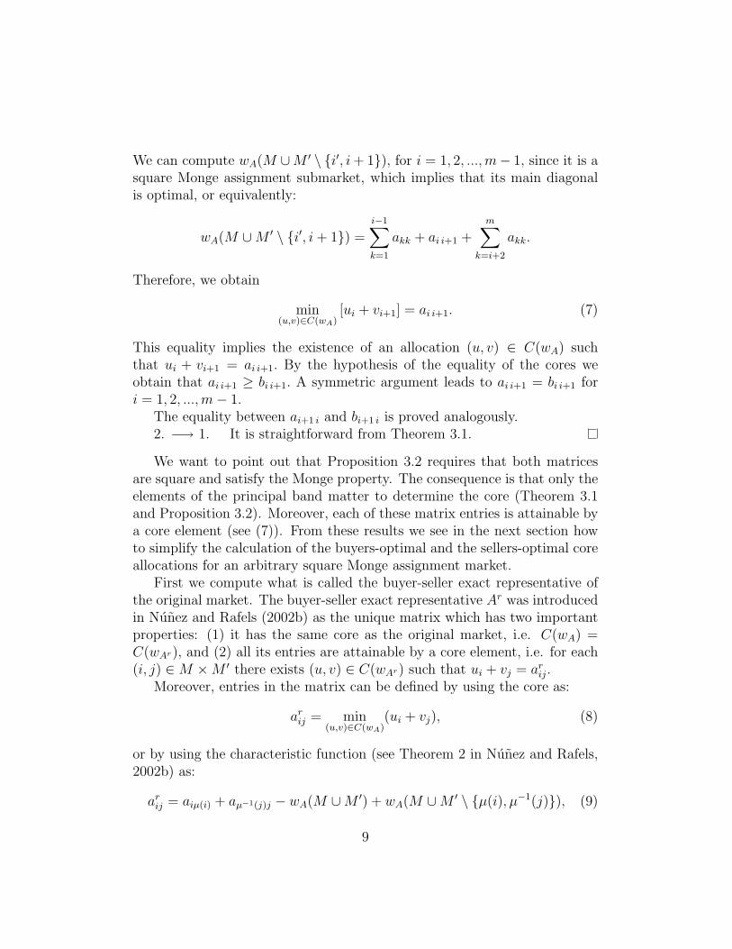
We can compute wA(M ∪M ′ \ {i′, i+ 1}), for i = 1, 2, ...,m− 1, since it is asquare Monge assignment submarket, which implies that its main diagonalis optimal, or equivalently:

wA(M ∪M ′ \ {i′, i+ 1}) =i−1∑k=1

akk + ai i+1 +m∑

k=i+2

akk.

Therefore, we obtain

min(u,v)∈C(wA)

[ui + vi+1] = ai i+1. (7)

This equality implies the existence of an allocation (u, v) ∈ C(wA) suchthat ui + vi+1 = ai i+1. By the hypothesis of the equality of the cores weobtain that ai i+1 ≥ bi i+1. A symmetric argument leads to ai i+1 = bi i+1 fori = 1, 2, ...,m− 1.

The equality between ai+1 i and bi+1 i is proved analogously.2. −→ 1. It is straightforward from Theorem 3.1.

We want to point out that Proposition 3.2 requires that both matricesare square and satisfy the Monge property. The consequence is that only theelements of the principal band matter to determine the core (Theorem 3.1and Proposition 3.2). Moreover, each of these matrix entries is attainable bya core element (see (7)). From these results we see in the next section howto simplify the calculation of the buyers-optimal and the sellers-optimal coreallocations for an arbitrary square Monge assignment market.

First we compute what is called the buyer-seller exact representative ofthe original market. The buyer-seller exact representative Ar was introducedin Nunez and Rafels (2002b) as the unique matrix which has two importantproperties: (1) it has the same core as the original market, i.e. C(wA) =C(wAr), and (2) all its entries are attainable by a core element, i.e. for each(i, j) ∈M ×M ′ there exists (u, v) ∈ C(wAr) such that ui + vj = arij.

Moreover, entries in the matrix can be defined by using the core as:

arij = min(u,v)∈C(wA)

(ui + vj), (8)

or by using the characteristic function (see Theorem 2 in Nunez and Rafels,2002b) as:

arij = aiµ(i) + aµ−1(j)j − wA(M ∪M ′) + wA(M ∪M ′ \ {µ(i), µ−1(j)}), (9)

9

for any optimal matching µ ∈M∗A(M,M ′), when matrix A is square.

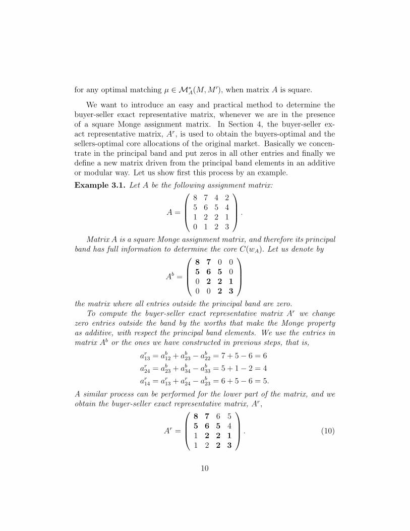
We want to introduce an easy and practical method to determine thebuyer-seller exact representative matrix, whenever we are in the presenceof a square Monge assignment matrix. In Section 4, the buyer-seller ex-act representative matrix, Ar, is used to obtain the buyers-optimal and thesellers-optimal core allocations of the original market. Basically we concen-trate in the principal band and put zeros in all other entries and finally wedefine a new matrix driven from the principal band elements in an additiveor modular way. Let us show first this process by an example.

Example 3.1. Let A be the following assignment matrix:

A =

8 7 4 25 6 5 41 2 2 10 1 2 3

.

Matrix A is a square Monge assignment matrix, and therefore its principalband has full information to determine the core C(wA). Let us denote by

Ab =

8 7 0 05 6 5 00 2 2 10 0 2 3

the matrix where all entries outside the principal band are zero.

To compute the buyer-seller exact representative matrix Ar we changezero entries outside the band by the worths that make the Monge propertyas additive, with respect the principal band elements. We use the entries inmatrix Ab or the ones we have constructed in previous steps, that is,

ar13 = ab12 + ab23 − ab22 = 7 + 5− 6 = 6

ar24 = ab23 + ab34 − ab33 = 5 + 1− 2 = 4

ar14 = ar13 + ar24 − ab23 = 6 + 5− 6 = 5.

A similar process can be performed for the lower part of the matrix, and weobtain the buyer-seller exact representative matrix, Ar,

Ar =

8 7 6 55 6 5 41 2 2 11 2 2 3

. (10)

10

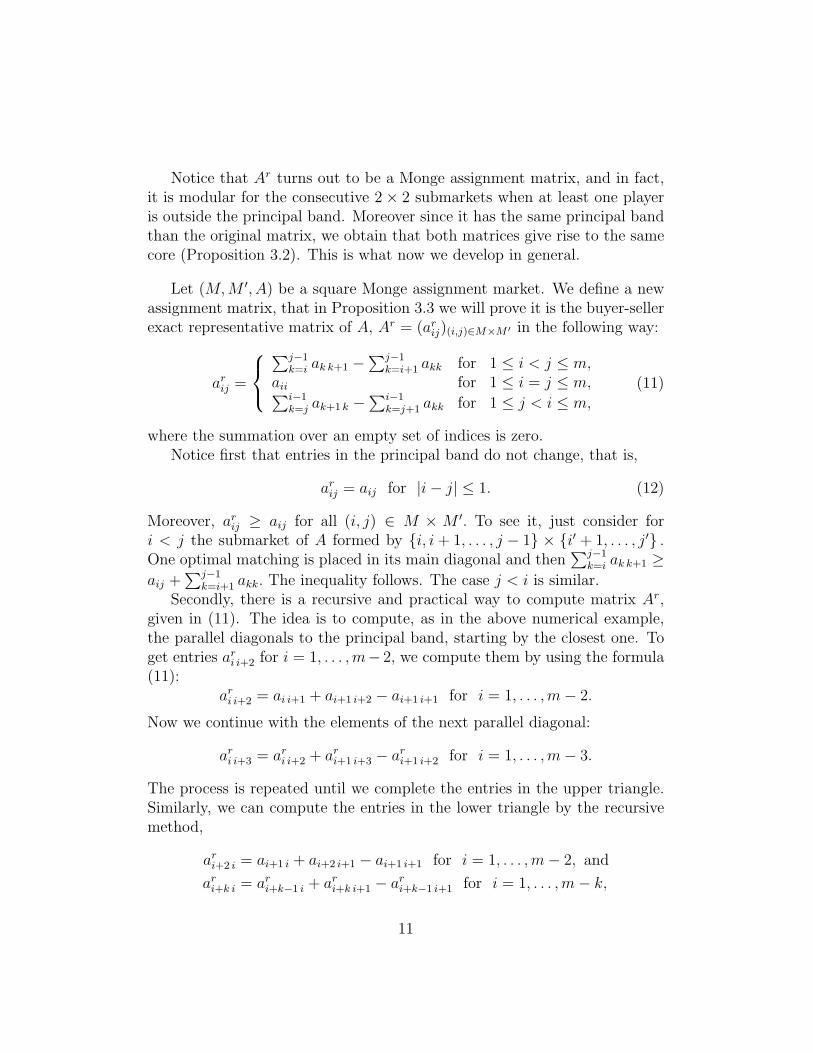
Notice that Ar turns out to be a Monge assignment matrix, and in fact,it is modular for the consecutive 2× 2 submarkets when at least one playeris outside the principal band. Moreover since it has the same principal bandthan the original matrix, we obtain that both matrices give rise to the samecore (Proposition 3.2). This is what now we develop in general.

Let (M,M ′, A) be a square Monge assignment market. We define a newassignment matrix, that in Proposition 3.3 we will prove it is the buyer-sellerexact representative matrix of A, Ar = (arij)(i,j)∈M×M ′ in the following way:

arij =

∑j−1

k=i ak k+1 −∑j−1

k=i+1 akk for 1 ≤ i < j ≤ m,aii for 1 ≤ i = j ≤ m,∑i−1

k=j ak+1 k −∑i−1

k=j+1 akk for 1 ≤ j < i ≤ m,

(11)

where the summation over an empty set of indices is zero.Notice first that entries in the principal band do not change, that is,

arij = aij for |i− j| ≤ 1. (12)

Moreover, arij ≥ aij for all (i, j) ∈ M × M ′. To see it, just consider fori < j the submarket of A formed by {i, i+ 1, . . . , j − 1} × {i′ + 1, . . . , j′} .One optimal matching is placed in its main diagonal and then

∑j−1k=i ak k+1 ≥

aij +∑j−1

k=i+1 akk. The inequality follows. The case j < i is similar.Secondly, there is a recursive and practical way to compute matrix Ar,

given in (11). The idea is to compute, as in the above numerical example,the parallel diagonals to the principal band, starting by the closest one. Toget entries ari i+2 for i = 1, . . . ,m− 2, we compute them by using the formula(11):

ari i+2 = ai i+1 + ai+1 i+2 − ai+1 i+1 for i = 1, . . . ,m− 2.

Now we continue with the elements of the next parallel diagonal:

ari i+3 = ari i+2 + ari+1 i+3 − ari+1 i+2 for i = 1, . . . ,m− 3.

The process is repeated until we complete the entries in the upper triangle.Similarly, we can compute the entries in the lower triangle by the recursivemethod,

ari+2 i = ai+1 i + ai+2 i+1 − ai+1 i+1 for i = 1, . . . ,m− 2, and

ari+k i = ari+k−1 i + ari+k i+1 − ari+k−1 i+1 for i = 1, . . . ,m− k,

11

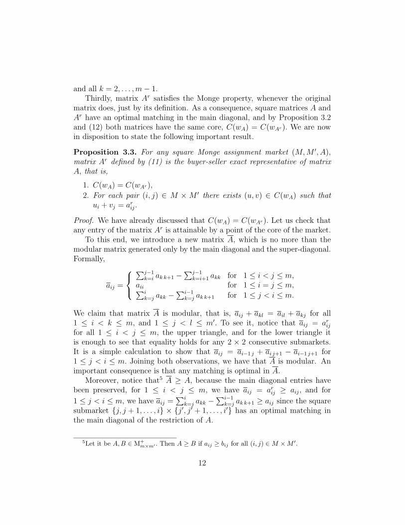
and all k = 2, . . . ,m− 1.Thirdly, matrix Ar satisfies the Monge property, whenever the original

matrix does, just by its definition. As a consequence, square matrices A andAr have an optimal matching in the main diagonal, and by Proposition 3.2and (12) both matrices have the same core, C(wA) = C(wAr). We are nowin disposition to state the following important result.

Proposition 3.3. For any square Monge assignment market (M,M ′, A),matrix Ar defined by (11) is the buyer-seller exact representative of matrixA, that is,

1. C(wA) = C(wAr),

2. For each pair (i, j) ∈ M ×M ′ there exists (u, v) ∈ C(wA) such thatui + vj = arij.

Proof. We have already discussed that C(wA) = C(wAr). Let us check thatany entry of the matrix Ar is attainable by a point of the core of the market.

To this end, we introduce a new matrix A, which is no more than themodular matrix generated only by the main diagonal and the super-diagonal.Formally,

aij =

∑j−1

k=i ak k+1 −∑j−1

k=i+1 akk for 1 ≤ i < j ≤ m,aii for 1 ≤ i = j ≤ m,∑i

k=j akk −∑i−1

k=j ak k+1 for 1 ≤ j < i ≤ m.

We claim that matrix A is modular, that is, aij + akl = ail + akj for all1 ≤ i < k ≤ m, and 1 ≤ j < l ≤ m′. To see it, notice that aij = arijfor all 1 ≤ i < j ≤ m, the upper triangle, and for the lower triangle itis enough to see that equality holds for any 2 × 2 consecutive submarkets.It is a simple calculation to show that aij = ai−1 j + ai j+1 − ai−1 j+1 for1 ≤ j < i ≤ m. Joining both observations, we have that A is modular. Animportant consequence is that any matching is optimal in A.

Moreover, notice that5 A ≥ A, because the main diagonal entries havebeen preserved, for 1 ≤ i < j ≤ m, we have aij = arij ≥ aij, and for

1 ≤ j < i ≤ m, we have aij =∑i

k=j akk −∑i−1

k=j ak k+1 ≥ aij since the squaresubmarket {j, j + 1, . . . , i} × {j′, j′ + 1, . . . , i′} has an optimal matching inthe main diagonal of the restriction of A.

5Let it be A, B ∈ M+m×m′ . Then A ≥ B if aij ≥ bij for all (i, j) ∈M ×M ′.

12

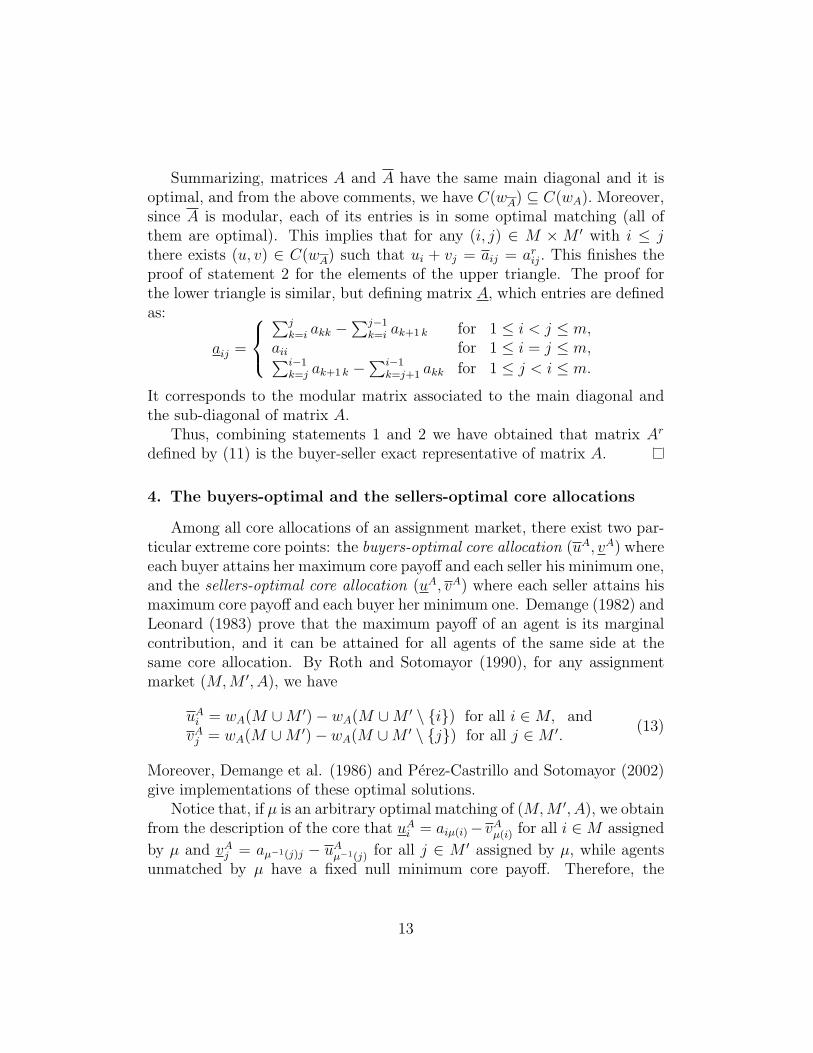
Summarizing, matrices A and A have the same main diagonal and it isoptimal, and from the above comments, we have C(wA) ⊆ C(wA). Moreover,since A is modular, each of its entries is in some optimal matching (all ofthem are optimal). This implies that for any (i, j) ∈ M ×M ′ with i ≤ jthere exists (u, v) ∈ C(wA) such that ui + vj = aij = arij. This finishes theproof of statement 2 for the elements of the upper triangle. The proof forthe lower triangle is similar, but defining matrix A, which entries are definedas:

aij =

∑j

k=i akk −∑j−1

k=i ak+1 k for 1 ≤ i < j ≤ m,aii for 1 ≤ i = j ≤ m,∑i−1

k=j ak+1 k −∑i−1

k=j+1 akk for 1 ≤ j < i ≤ m.

It corresponds to the modular matrix associated to the main diagonal andthe sub-diagonal of matrix A.

Thus, combining statements 1 and 2 we have obtained that matrix Ar

defined by (11) is the buyer-seller exact representative of matrix A.

4. The buyers-optimal and the sellers-optimal core allocations

Among all core allocations of an assignment market, there exist two par-ticular extreme core points: the buyers-optimal core allocation (uA, vA) whereeach buyer attains her maximum core payoff and each seller his minimum one,and the sellers-optimal core allocation (uA, vA) where each seller attains hismaximum core payoff and each buyer her minimum one. Demange (1982) andLeonard (1983) prove that the maximum payoff of an agent is its marginalcontribution, and it can be attained for all agents of the same side at thesame core allocation. By Roth and Sotomayor (1990), for any assignmentmarket (M,M ′, A), we have

uAi = wA(M ∪M ′)− wA(M ∪M ′ \ {i}) for all i ∈M, andvAj = wA(M ∪M ′)− wA(M ∪M ′ \ {j}) for all j ∈M ′.

(13)

Moreover, Demange et al. (1986) and Perez-Castrillo and Sotomayor (2002)give implementations of these optimal solutions.

Notice that, if µ is an arbitrary optimal matching of (M,M ′, A), we obtainfrom the description of the core that uAi = aiµ(i)−vAµ(i) for all i ∈M assigned

by µ and vAj = aµ−1(j)j − uAµ−1(j) for all j ∈ M ′ assigned by µ, while agentsunmatched by µ have a fixed null minimum core payoff. Therefore, the

13

minimum core payoffs for a sector are determined by knowing an optimalmatching and the maximum core payoffs of the other sector.

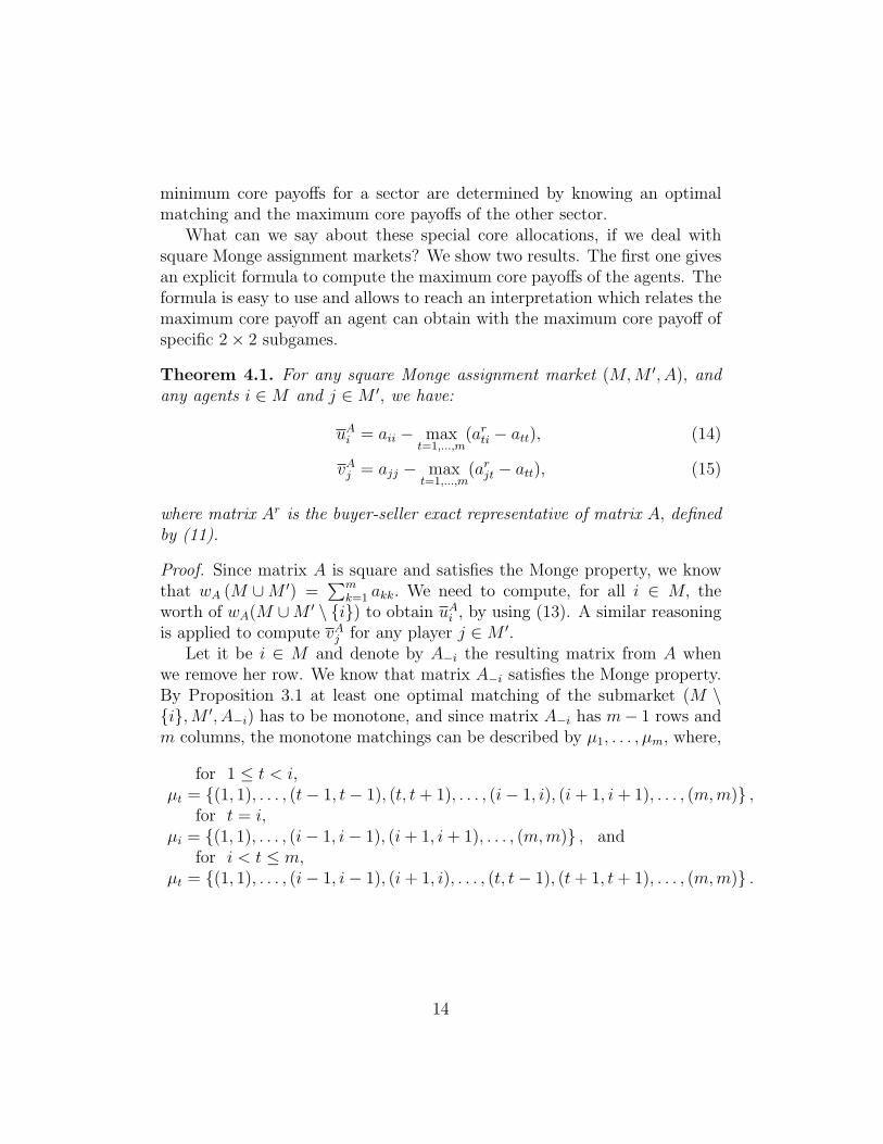
What can we say about these special core allocations, if we deal withsquare Monge assignment markets? We show two results. The first one givesan explicit formula to compute the maximum core payoffs of the agents. Theformula is easy to use and allows to reach an interpretation which relates themaximum core payoff an agent can obtain with the maximum core payoff ofspecific 2× 2 subgames.

Theorem 4.1. For any square Monge assignment market (M,M ′, A), andany agents i ∈M and j ∈M ′, we have:

uAi = aii − maxt=1,...,m

(arti − att), (14)

vAj = ajj − maxt=1,...,m

(arjt − att), (15)

where matrix Ar is the buyer-seller exact representative of matrix A, definedby (11).

Proof. Since matrix A is square and satisfies the Monge property, we knowthat wA (M ∪M ′) =

∑mk=1 akk. We need to compute, for all i ∈ M, the

worth of wA(M ∪M ′ \ {i}) to obtain uAi , by using (13). A similar reasoningis applied to compute vAj for any player j ∈M ′.

Let it be i ∈ M and denote by A−i the resulting matrix from A whenwe remove her row. We know that matrix A−i satisfies the Monge property.By Proposition 3.1 at least one optimal matching of the submarket (M \{i},M ′, A−i) has to be monotone, and since matrix A−i has m− 1 rows andm columns, the monotone matchings can be described by µ1, . . . , µm, where,

for 1 ≤ t < i,µt = {(1, 1), . . . , (t− 1, t− 1), (t, t+ 1), . . . , (i− 1, i), (i+ 1, i+ 1), . . . , (m,m)} ,

for t = i,µi = {(1, 1), . . . , (i− 1, i− 1), (i+ 1, i+ 1), . . . , (m,m)} , and

for i < t ≤ m,µt = {(1, 1), . . . , (i− 1, i− 1), (i+ 1, i), . . . , (t, t− 1), (t+ 1, t+ 1), . . . , (m,m)} .

14

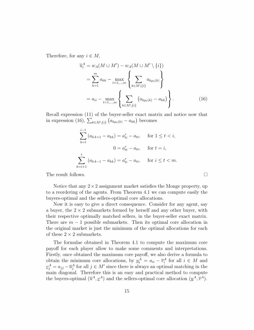
Therefore, for any i ∈M,

uAi = wA(M ∪M ′)− wA(M ∪M ′ \ {i})

=m∑k=1

akk − maxt=1,...,m

∑k∈M\{i}

akµt(k)

= aii − max

t=1,...,m

∑k∈M\{i}

(akµt(k) − akk

) . (16)

Recall expression (11) of the buyer-seller exact matrix and notice now thatin expression (16),

∑k∈M\{i}

(akµt(k) − akk

)becomes

i−1∑k=t

(ak k+1 − akk) = arti − att, for 1 ≤ t < i,

0 = artt − att, for t = i,t∑

k=i+1

(ak k−1 − akk) = arti − att, for i ≤ t < m.

The result follows.

Notice that any 2×2 assignment market satisfies the Monge property, upto a reordering of the agents. From Theorem 4.1 we can compute easily thebuyers-optimal and the sellers-optimal core allocations.

Now it is easy to give a direct consequence. Consider for any agent, saya buyer, the 2 × 2 submarkets formed by herself and any other buyer, withtheir respective optimally matched sellers, in the buyer-seller exact matrix.There are m − 1 possible submarkets. Then its optimal core allocation inthe original market is just the minimum of the optimal allocations for eachof these 2× 2 submarkets.

The formulae obtained in Theorem 4.1 to compute the maximum corepayoff for each player allow to make some comments and interpretations.Firstly, once obtained the maximum core payoff, we also derive a formula toobtain the minimum core allocations, by uAi = aii − vAi for all i ∈ M andvAj = ajj−uAj for all j ∈M ′ since there is always an optimal matching in themain diagonal. Therefore this is an easy and practical method to computethe buyers-optimal (uA, vA) and the sellers-optimal core allocation (uA, vA).

15

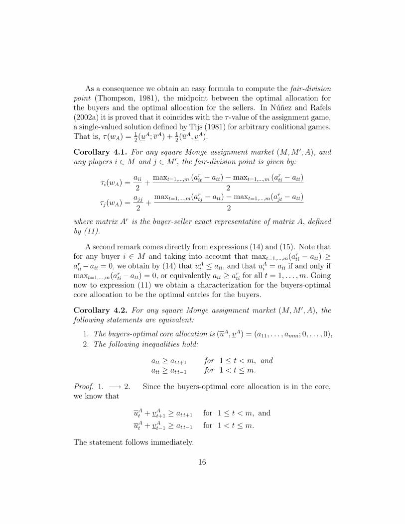
As a consequence we obtain an easy formula to compute the fair-divisionpoint (Thompson, 1981), the midpoint between the optimal allocation forthe buyers and the optimal allocation for the sellers. In Nunez and Rafels(2002a) it is proved that it coincides with the τ -value of the assignment game,a single-valued solution defined by Tijs (1981) for arbitrary coalitional games.That is, τ(wA) = 1

2(uA; vA) + 1

2(uA, vA).

Corollary 4.1. For any square Monge assignment market (M,M ′, A), andany players i ∈M and j ∈M ′, the fair-division point is given by:

τi(wA) =aii2

+maxt=1,...,m (arit − att)−maxt=1,...,m (arti − att)

2

τj(wA) =ajj2

+maxt=1,...,m(artj − att)−maxt=1,...,m(arjt − att)

2

where matrix Ar is the buyer-seller exact representative of matrix A, definedby (11).

A second remark comes directly from expressions (14) and (15). Note thatfor any buyer i ∈ M and taking into account that maxt=1,...,m(arti − att) ≥arii−aii = 0, we obtain by (14) that uAi ≤ aii, and that uAi = aii if and only ifmaxt=1,...,m(arti− att) = 0, or equivalently att ≥ arti for all t = 1, . . . ,m. Goingnow to expression (11) we obtain a characterization for the buyers-optimalcore allocation to be the optimal entries for the buyers.

Corollary 4.2. For any square Monge assignment market (M,M ′, A), thefollowing statements are equivalent:

1. The buyers-optimal core allocation is (uA, vA) = (a11, . . . , amm; 0, . . . , 0),

2. The following inequalities hold:

att ≥ at t+1 for 1 ≤ t < m, andatt ≥ at t−1 for 1 < t ≤ m.

Proof. 1. −→ 2. Since the buyers-optimal core allocation is in the core,we know that

uAt + vAt+1 ≥ at t+1 for 1 ≤ t < m, and

uAt + vAt−1 ≥ at t−1 for 1 < t ≤ m.

The statement follows immediately.

16

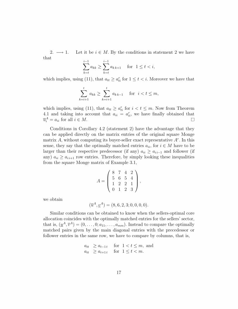
2. −→ 1. Let it be i ∈ M. By the conditions in statement 2 we havethat

i−1∑k=t

akk ≥i−1∑k=t

ak k+1 for 1 ≤ t < i,

which implies, using (11), that att ≥ arti for 1 ≤ t < i. Moreover we have that

t∑k=i+1

akk ≥t∑

k=i+1

ak k−1 for i < t ≤ m,

which implies, using (11), that att ≥ arti for i < t ≤ m. Now from Theorem4.1 and taking into account that aii = arii, we have finally obtained thatuAi = aii for all i ∈M.

Conditions in Corollary 4.2 (statement 2) have the advantage that theycan be applied directly on the matrix entries of the original square Mongematrix A, without computing its buyer-seller exact representative Ar. In thissense, they say that the optimally matched entries aii, for i ∈M have to belarger than their respective predecessor (if any) aii ≥ ai i−1 and follower (ifany) aii ≥ ai i+1 row entries. Therefore, by simply looking these inequalitiesfrom the square Monge matrix of Example 3.1,

A =

8 7 4 25 6 5 41 2 2 10 1 2 3

,

we obtain(uA, vA) = (8, 6, 2, 3; 0, 0, 0, 0).

Similar conditions can be obtained to know when the sellers-optimal coreallocation coincides with the optimally matched entries for the sellers’ sector,that is, (uA, vA) = (0, . . . , 0; a11, . . . , amm). Instead to compare the optimallymatched pairs given by the main diagonal entries with the precedessor orfollower entries in the same row, we have to compare by columns, that is,

att ≥ at−1 t for 1 < t ≤ m, andatt ≥ at+1 t for 1 ≤ t < m.

17

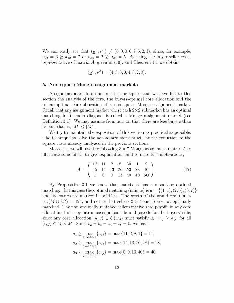
We can easily see that (uA, vA) 6= (0, 0, 0, 0; 8, 6, 2, 3), since, for example,a22 = 6 � a12 = 7 or a33 = 2 � a23 = 5. By using the buyer-seller exactrepresentative of matrix A, given in (10), and Theorem 4.1 we obtain

(uA, vA) = (4, 3, 0, 0; 4, 3, 2, 3).

5. Non-square Monge assignment markets

Assignment markets do not need to be square and we have left to thissection the analysis of the core, the buyers-optimal core allocation and thesellers-optimal core allocation of a non-square Monge assignment market.Recall that any assignment market where each 2×2 submarket has an optimalmatching in its main diagonal is called a Monge assignment market (seeDefinition 3.1). We may assume from now on that there are less buyers thansellers, that is, |M | ≤ |M ′|.

We try to maintain the exposition of this section as practical as possible.The technique to solve the non-square markets will be the reduction to thesquare cases already analyzed in the previous sections.

Moreover, we will use the following 3× 7 Monge assignment matrix A toillustrate some ideas, to give explanations and to introduce motivations,

A =

12 11 2 8 30 1 915 14 13 26 52 28 401 0 0 13 40 40 60

. (17)

By Proposition 3.1 we know that matrix A has a monotone optimalmatching. In this case the optimal matching (unique) is µ = {(1, 1), (2, 5), (3, 7)}and its entries are marked in boldface. The worth of the grand coalition iswA(M ∪M ′) = 124, and notice that sellers 2, 3, 4 and 6 are not optimallymatched. The non-optimally matched sellers receive zero payoffs in any coreallocation, but they introduce significant bound payoffs for the buyers’ side,since any core allocation (u, v) ∈ C(wA) must satisfy ui + vj ≥ aij, for all(i, j) ∈M ×M ′. Since v2 = v3 = v4 = v6 = 0, we have,

u1 ≥ maxj=2,3,4,6

{a1j} = max{11, 2, 8, 1} = 11,

u2 ≥ maxj=2,3,4,6

{a2j} = max{14, 13, 26, 28} = 28,

u3 ≥ maxj=2,3,4,6

{a3j} = max{0, 0, 13, 40} = 40.

18

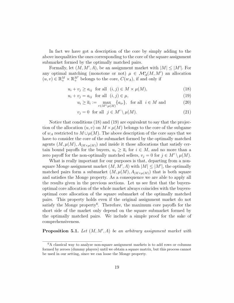
In fact we have got a description of the core by simply adding to theabove inequalities the ones corresponding to the core of the square assignmentsubmarket formed by the optimally matched pairs.

Formally, let (M,M ′, A), be an assignment market with |M | ≤ |M ′|. Forany optimal matching (monotone or not) µ ∈ M∗

A(M,M ′) an allocation(u, v) ∈ RM+ × RM

′+ belongs to the core, C(wA), if and only if

ui + vj ≥ aij for all (i, j) ∈M × µ(M), (18)

ui + vj = aij for all (i, j) ∈ µ, (19)

ui ≥ ai := maxr∈M ′\µ(M)

{air}, for all i ∈M and (20)

vj = 0 for all j ∈M ′ \ µ(M). (21)

Notice that conditions (18) and (19) are equivalent to say that the projec-tion of the allocation (u, v) on M ×µ(M) belongs to the core of the subgameof wA restricted to M ∪µ(M). The above description of the core says that wehave to consider the core of the submarket formed by the optimally matchedagents (M,µ(M), A|M×µ(M)) and inside it those allocations that satisfy cer-tain bound payoffs for the buyers, ui ≥ ai for i ∈ M, and no more than azero payoff for the non-optimally matched sellers, vj = 0 for j ∈M ′ \ µ(M).

What is really important for our purposes is that, departing from a non-square Monge assignment market (M,M ′, A) with |M | ≤ |M ′|, the optimallymatched pairs form a submarket (M,µ(M), A|M×µ(M)) that is both squareand satisfies the Monge property. As a consequence we are able to apply allthe results given in the previous sections. Let us see first that the buyers-optimal core allocation of the whole market always coincides with the buyers-optimal core allocation of the square submarket of the optimally matchedpairs. This property holds even if the original assignment market do notsatisfy the Monge property6. Therefore, the maximum core payoffs for theshort side of the market only depend on the square submarket formed bythe optimally matched pairs. We include a simple proof for the sake ofcomprehensiveness.

Proposition 5.1. Let (M,M ′, A) be an arbitrary assignment market with

6A classical way to analyze non-square assignment markets is to add rows or columnsformed by zeroes (dummy players) until we obtain a square matrix, but this process cannotbe used in our setting, since we can loose the Monge property.

19

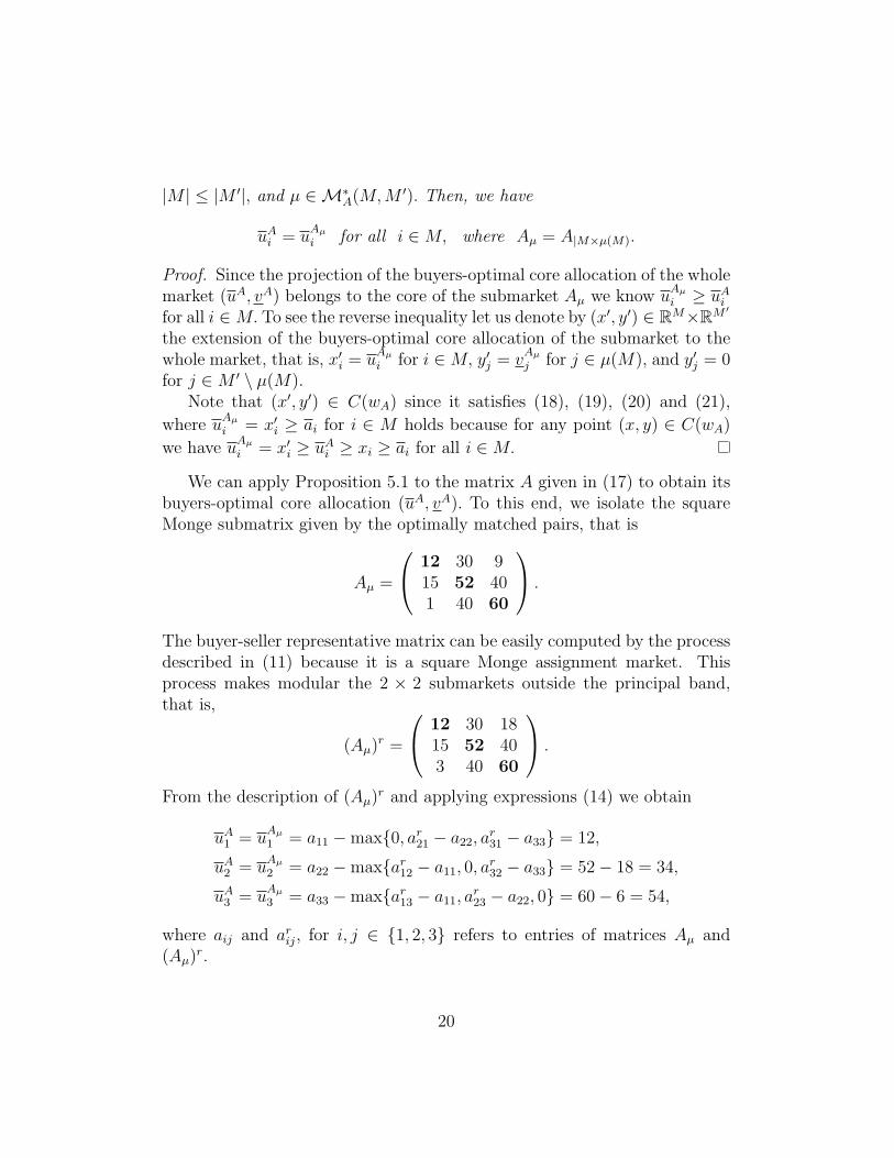
|M | ≤ |M ′|, and µ ∈M∗A(M,M ′). Then, we have

uAi = uAµi for all i ∈M, where Aµ = A|M×µ(M).

Proof. Since the projection of the buyers-optimal core allocation of the wholemarket (uA, vA) belongs to the core of the submarket Aµ we know u

Aµi ≥ uAi

for all i ∈M. To see the reverse inequality let us denote by (x′, y′) ∈ RM×RM ′

the extension of the buyers-optimal core allocation of the submarket to thewhole market, that is, x′i = u

Aµi for i ∈M, y′j = v

Aµj for j ∈ µ(M), and y′j = 0

for j ∈M ′ \ µ(M).Note that (x′, y′) ∈ C(wA) since it satisfies (18), (19), (20) and (21),

where uAµi = x′i ≥ ai for i ∈ M holds because for any point (x, y) ∈ C(wA)

we have uAµi = x′i ≥ uAi ≥ xi ≥ ai for all i ∈M.

We can apply Proposition 5.1 to the matrix A given in (17) to obtain itsbuyers-optimal core allocation (uA, vA). To this end, we isolate the squareMonge submatrix given by the optimally matched pairs, that is

Aµ =

12 30 915 52 401 40 60

.

The buyer-seller representative matrix can be easily computed by the processdescribed in (11) because it is a square Monge assignment market. Thisprocess makes modular the 2 × 2 submarkets outside the principal band,that is,

(Aµ)r =

12 30 1815 52 403 40 60

.

From the description of (Aµ)r and applying expressions (14) we obtain

uA1 = uAµ1 = a11 −max{0, ar21 − a22, a

r31 − a33} = 12,

uA2 = uAµ2 = a22 −max{ar12 − a11, 0, a

r32 − a33} = 52− 18 = 34,

uA3 = uAµ3 = a33 −max{ar13 − a11, a

r23 − a22, 0} = 60− 6 = 54,

where aij and arij, for i, j ∈ {1, 2, 3} refers to entries of matrices Aµ and(Aµ)r.

20

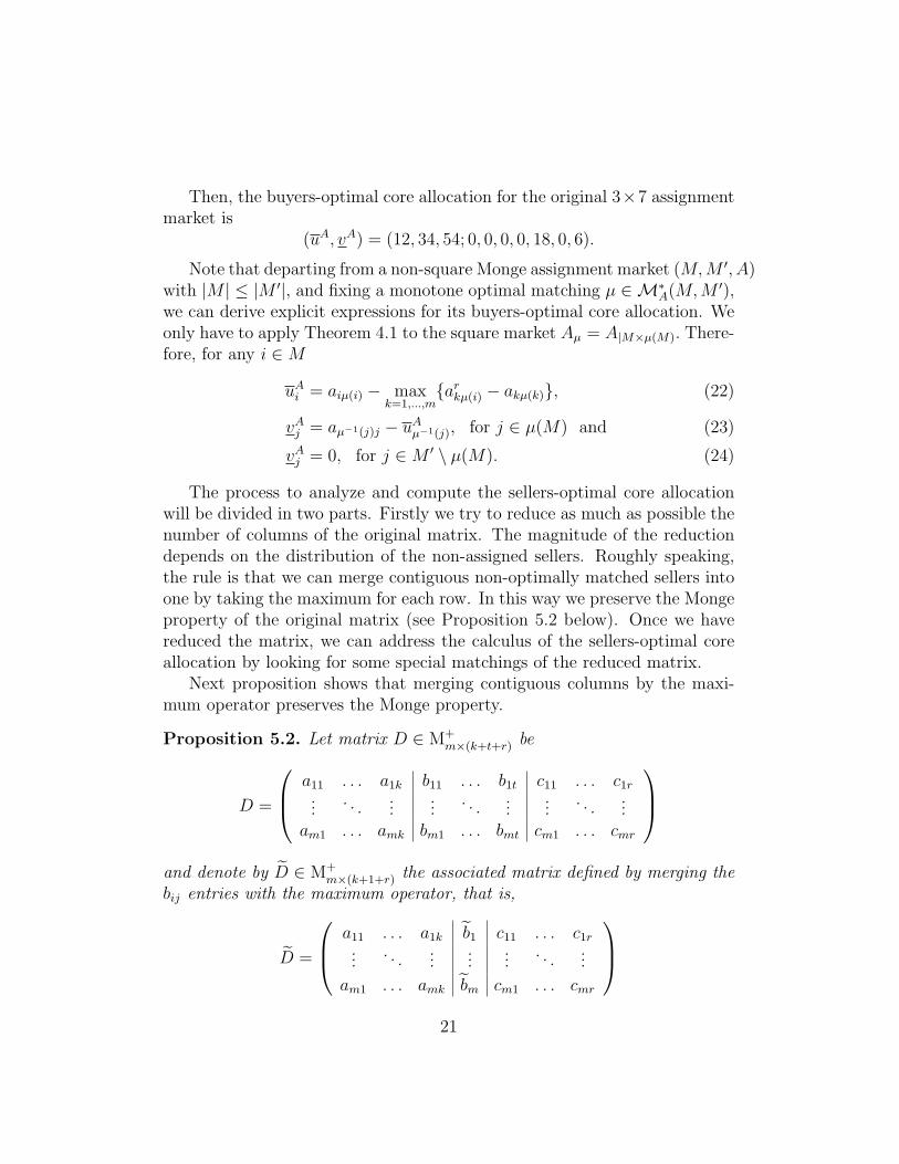
Then, the buyers-optimal core allocation for the original 3×7 assignmentmarket is

(uA, vA) = (12, 34, 54; 0, 0, 0, 0, 18, 0, 6).

Note that departing from a non-square Monge assignment market (M,M ′, A)with |M | ≤ |M ′|, and fixing a monotone optimal matching µ ∈M∗

A(M,M ′),we can derive explicit expressions for its buyers-optimal core allocation. Weonly have to apply Theorem 4.1 to the square market Aµ = A|M×µ(M). There-fore, for any i ∈M

uAi = aiµ(i) − maxk=1,...,m

{arkµ(i) − akµ(k)}, (22)

vAj = aµ−1(j)j − uAµ−1(j), for j ∈ µ(M) and (23)

vAj = 0, for j ∈M ′ \ µ(M). (24)

The process to analyze and compute the sellers-optimal core allocationwill be divided in two parts. Firstly we try to reduce as much as possible thenumber of columns of the original matrix. The magnitude of the reductiondepends on the distribution of the non-assigned sellers. Roughly speaking,the rule is that we can merge contiguous non-optimally matched sellers intoone by taking the maximum for each row. In this way we preserve the Mongeproperty of the original matrix (see Proposition 5.2 below). Once we havereduced the matrix, we can address the calculus of the sellers-optimal coreallocation by looking for some special matchings of the reduced matrix.

Next proposition shows that merging contiguous columns by the maxi-mum operator preserves the Monge property.

Proposition 5.2. Let matrix D ∈ M+m×(k+t+r) be

D =

a11 . . . a1k b11 . . . b1t c11 . . . c1r...

. . ....

.... . .

......

. . ....

am1 . . . amk bm1 . . . bmt cm1 . . . cmr

and denote by D ∈ M+

m×(k+1+r) the associated matrix defined by merging thebij entries with the maximum operator, that is,

D =

a11 . . . a1k b1 c11 . . . c1r...

. . ....

......

. . ....

am1 . . . amk bm cm1 . . . cmr

21

where bi = maxl=1,...,t{bil} for i = 1, 2, . . . ,m. Then, if D satisfies the Monge

property, matrix D does also.

Proof. We only have to prove that the 2× 2 submatrices of the form(aik biai+1 k bi+1

)or

(bi ci1bi+1 ci+11

)for i = 1, . . . ,m− 1.

have an optimal matching in its main diagonal.We only prove the statement for the first type of submatrix, since the

other one can be proved similarly. Notice first that bi = bir∗ for some r∗, 1 ≤r∗ ≤ t. Then,

aik + bi+1 = aik + maxl=1,...,t

{bi+1 l} ≥ aik + bi+1 r∗ ≥ ai+1 k + bir∗ = ai+1 k + bi,

where the last inequality comes from the fact that matrix D satisfies theMonge property.

We can apply Proposition 5.2 to our 3×7 matrix A given in (17) to reducethe sellers’ sector, merging sellers 2, 3 and 4 in a unique column obtaining a3× 5 Monge assignment market (M, M ′, A), with

A =

12 11 30 1 915 26 52 28 401 13 40 40 60

. (25)

As the original non-optimally matched sellers get a zero payoff in anycore allocation, we already know that vA2 = vA3 = vA4 = vA6 = 0. Let usthen concentrate on the rest of the sellers, that is, vA1 , v

A5 and vA7 . These

worths now correspond, in the reduced matrix A with vA1 , vA3 and vA5 , and

vA1 = vA1 , vA5 = vA3 and vA7 = vA5 , since the core of the assignment markets

given by matrix A and A are alike, and differ just by the dimension spaceswhere they are in and also in the numeration of the players. This is so becausewe have merged non-optimally matched sellers of the original assignmentmarket by the maximum operator and this fact essentially does not changethe core, for the original optimally matched pairs (see (18), (19 ) and ( 20)).Notice that the entries of the optimal matching will be preserved, from A toA.

22

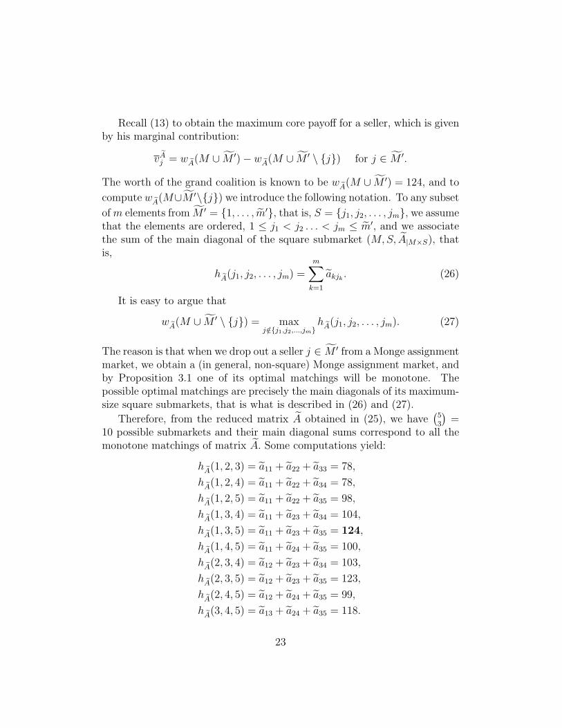
Recall (13) to obtain the maximum core payoff for a seller, which is givenby his marginal contribution:

vAj = wA(M ∪ M ′)− wA(M ∪ M ′ \ {j}) for j ∈ M ′.

The worth of the grand coalition is known to be wA(M ∪ M ′) = 124, and to

compute wA(M∪M ′\{j}) we introduce the following notation. To any subset

of m elements from M ′ = {1, . . . , m′}, that is, S = {j1, j2, . . . , jm}, we assumethat the elements are ordered, 1 ≤ j1 < j2 . . . < jm ≤ m′, and we associatethe sum of the main diagonal of the square submarket (M,S, A|M×S), thatis,

hA(j1, j2, . . . , jm) =m∑k=1

akjk . (26)

It is easy to argue that

wA(M ∪ M ′ \ {j}) = maxj /∈{j1,j2,...,jm}

hA(j1, j2, . . . , jm). (27)

The reason is that when we drop out a seller j ∈ M ′ from a Monge assignmentmarket, we obtain a (in general, non-square) Monge assignment market, andby Proposition 3.1 one of its optimal matchings will be monotone. Thepossible optimal matchings are precisely the main diagonals of its maximum-size square submarkets, that is what is described in (26) and (27).

Therefore, from the reduced matrix A obtained in (25), we have(53

)=

10 possible submarkets and their main diagonal sums correspond to all themonotone matchings of matrix A. Some computations yield:

hA(1, 2, 3) = a11 + a22 + a33 = 78,

hA(1, 2, 4) = a11 + a22 + a34 = 78,

hA(1, 2, 5) = a11 + a22 + a35 = 98,

hA(1, 3, 4) = a11 + a23 + a34 = 104,

hA(1, 3, 5) = a11 + a23 + a35 = 124,

hA(1, 4, 5) = a11 + a24 + a35 = 100,

hA(2, 3, 4) = a12 + a23 + a34 = 103,

hA(2, 3, 5) = a12 + a23 + a35 = 123,

hA(2, 4, 5) = a12 + a24 + a35 = 99,

hA(3, 4, 5) = a13 + a24 + a35 = 118.

23

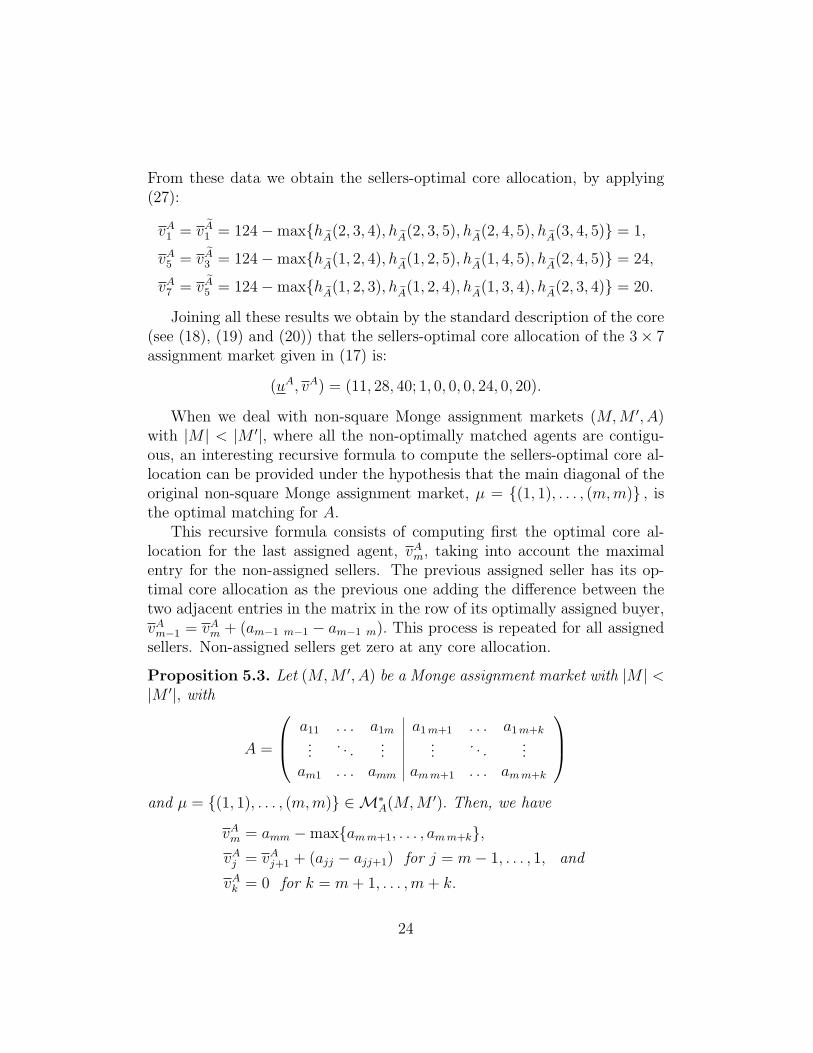
From these data we obtain the sellers-optimal core allocation, by applying(27):

vA1 = vA1 = 124−max{hA(2, 3, 4), hA(2, 3, 5), hA(2, 4, 5), hA(3, 4, 5)} = 1,

vA5 = vA3 = 124−max{hA(1, 2, 4), hA(1, 2, 5), hA(1, 4, 5), hA(2, 4, 5)} = 24,

vA7 = vA5 = 124−max{hA(1, 2, 3), hA(1, 2, 4), hA(1, 3, 4), hA(2, 3, 4)} = 20.

Joining all these results we obtain by the standard description of the core(see (18), (19) and (20)) that the sellers-optimal core allocation of the 3× 7assignment market given in (17) is:

(uA, vA) = (11, 28, 40; 1, 0, 0, 0, 24, 0, 20).

When we deal with non-square Monge assignment markets (M,M ′, A)with |M | < |M ′|, where all the non-optimally matched agents are contigu-ous, an interesting recursive formula to compute the sellers-optimal core al-location can be provided under the hypothesis that the main diagonal of theoriginal non-square Monge assignment market, µ = {(1, 1), . . . , (m,m)} , isthe optimal matching for A.

This recursive formula consists of computing first the optimal core al-location for the last assigned agent, vAm, taking into account the maximalentry for the non-assigned sellers. The previous assigned seller has its op-timal core allocation as the previous one adding the difference between thetwo adjacent entries in the matrix in the row of its optimally assigned buyer,vAm−1 = vAm + (am−1 m−1 − am−1 m). This process is repeated for all assignedsellers. Non-assigned sellers get zero at any core allocation.

Proposition 5.3. Let (M,M ′, A) be a Monge assignment market with |M | <|M ′|, with

A =

a11 . . . a1m a1m+1 . . . a1m+k...

. . ....

.... . .

...am1 . . . amm amm+1 . . . amm+k

and µ = {(1, 1), . . . , (m,m)} ∈ M∗

A(M,M ′). Then, we have

vAm = amm −max{amm+1, . . . , amm+k},vAj = vAj+1 + (ajj − ajj+1) for j = m− 1, . . . , 1, and

vAk = 0 for k = m+ 1, . . . ,m+ k.

24

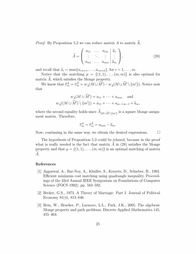
Proof. By Proposition 5.2 we can reduce matrix A to matrix A,

A =

a11 . . . a1m a1...

. . ....

...am1 . . . amm am

, (28)

and recall that ai = max{aim+1, . . . , aim+k}, for i = 1, . . . ,m.Notice that the matching µ = {(1, 1), . . . , (m,m)} is also optimal for

matrix A, which satisfies the Monge property.

We know that vAm = vAm = wA(M ∪M ′)−wA(M ∪M ′ \{m′}). Notice nowthat

wA(M ∪ M ′) = a11 + · · ·+ amm and

wA((M ∪ M ′) \ {m′}) = a11 + · · ·+ am−1m−1 + am,

where the second equality holds since A|M×M ′\{m′} is a square Monge assign-ment matrix. Therefore,

vAm = vAm = amm − am.

Now, continuing in the same way, we obtain the desired expressions.

The hypothesis of Proposition 5.3 could be relaxed, because in the proofwhat is really needed is the fact that matrix A in (28) satisfies the Mongeproperty and that µ = {(1, 1), . . . , (m,m)} is an optimal matching of matrix

A.

References

[1] Aggarwal, A., Bar-Noy, A., Khuller, S., Kravets, D., Schieber, B., 1992.Efficient minimum cost matching using quadrangle inequality. Proceed-ings of the 33rd Annual IEEE Symposium on Foundations of ComputerScience (FOCS 1992), pp. 583–592.

[2] Becker, G.S., 1973. A Theory of Marriage: Part I. Journal of PoliticalEconomy 81(4), 813–846.

[3] Bein, W., Brucker, P., Larmore, L.L., Park, J.K., 2005. The algebraicMonge property and path problems. Discrete Applied Mathematics 145,455–464.

25

[4] Burkard, R.E., 2007. Monge properties, discrete convexity and applica-tions. European Journal of Operational Research 176, 1–14.

[5] Burkard, R.E., Klinz, B., Rudiger, R., 1996. Perspectives of Monge prop-erties in optimization. Discrete Applied Mathematics 70, 95–161.

[6] Demange, G., 1982. Strategyproofness in the assignment market game.Laboratoire d’Econometrie de l’Ecole Polytechnique, Mimeo, Paris.

[7] Demange, G., Gale, D., Sotomayor, M., 1986. Multi-item auctions. Jour-nal of Political Economy 94, 863–872.

[8] Hoffman, A.J., 1963. On simple linear programming problems. In: Pro-ceedings of Symposia in Pure Mathematics, Convexity, Vol. VII, V. Klee,ed. AMS, Providence, RI, pp. 317–327.

[9] Hou, X., Prekopa, A., 2007. Monge property and bounding multivariateprobability distribution functions with given marginals and covariances.SIAM Journal on Optimization 18(1), 138–155.

[10] Leonard, H.B., 1983. Elicitation of honest preferences for the assignmentof individuals to positions. Journal of Political Economy 91, 461–479.

[11] Lin, J.Y., 1992. The Becker-Brock efficient matching with a supermod-ular technology defined on an n−lattice. Mathematical Social Sciences24, 105–109.

[12] Nunez, M., Rafels, C., 2002a. The assignment game: the tau value.International Journal of Game Theory 31, 411–422.

[13] Nunez, M., Rafels, C., 2002b. Buyer-seller exactness in the assignmentgame. International Journal of Game Theory 31, 423–436.

[14] Okamoto, Y., 2004. Traveling salesman games with the Monge property.Discrete Applied Mathematics 138, 349–369.

[15] Perez-Castrillo, D., Sotomayor, M., 2002. A simple selling and buyingprocedure. J Econ Theory 103, 461–474.

[16] Roth, A., Sotomayor, M., 1990. Two-sided matching. Econometric So-ciety Monographs, 18. Cambridge University Press.

26

[17] Shapley, L.S., Shubik, M., 1972. The Assignment Game I: The Core.International Journal of Game Theory 1, 111–130.

[18] Tijs, S.H., 1981. Bounds for the core and the τ–value. In: Game Theoryand Mathematical Economics, O. Moeschlin and D. Pallaschke, eds.North Holland Publishing Company, pp. 123–132.

[19] Thompson, G.L., 1981. Auctions and market games. In: Essays in GameTheory and Mathematical Economics in honor of Oskar Morgenstern,R. Aumann et al., eds. Bibliographisches Institute-WissenschaftsverlagMannheim, pp. 181–196.

27