departament de anàlisi matemàtica algebras de funciones analíticas
TRANSCRIPT
DEPARTAMENT DE ANÀLISI MATEMÀTICA ALGEBRAS DE FUNCIONES ANALÍTICAS ACOTADAS. INTERPOLACIÓN
ALEJANDRO MIRALLES MONTOLÍO
UNIVERSITAT DE VALÈNCIA Servei de Publicacions
2008

Aquesta Tesi Doctoral va ser presentada a València el dia 26 de juny de 2008 davant un tribunal format per:
- D. Richard M. Aron - D. Oscar Blasco de la Cruz - D. Mikael T. Lindström - Dª. Angeles Prieto Yerro - Dª. María Dolores Acosta Vigil
Va ser dirigida per: D. Pablo Galindo Pastor ©Copyright: Servei de Publicacions Alejandro Miralles Montolío
Depòsit legal: I.S.B.N.: 978-84-370-7251-7
Edita: Universitat de València Servei de Publicacions C/ Artes Gráficas, 13 bajo 46010 València Spain Telèfon: 963864115
ÁLGEBRAS DE FUNCIONES ANALÍTICASACOTADAS. INTERPOLACIÓN
ALEJANDRO MIRALLES MONTOLÍO
Tesis Doctoral dirigida por: PABLO GALINDO PASTOR
Valencia, Junio 2008
i

••ii
A mis padres
ii
Agradecimientos
Ahora, al echar la vista atrás, me llena un melancólico recuerdo cuando mis padresme cuentan que he llegado a ser todo lo que siempre dije que querría llegar a ser. Lasmatemáticas, los descubrimientos y los viajes son algo que se ha ido perfilando y adap-tando a través de los años pero, en definitiva, eso es justo lo que yo siempre deseé. Y, paraser sincero, el fruto de este trabajo es consecuencia de muchas cosas. Por una parte, lailusión por las matemáticas que siempre me ha acompañado y, por otra, las personas quehan hecho posible que esta ilusión no se desvaneciera.
Entre las personas que me han motivado a lo largo de estos años, quisiera destacarde forma muy especial el apoyo de mi director, Pablo Galindo. Su ayuda profesional ylos buenos consejos en cada momento han ido forjando la dirección correcta. A él le deboprincipalmente este trabajo.
Quiero destacar también la influencia de Richard Aron, a quien admiro en todos lossentidos. A él le debo parte de mi formación y de mis buenos momentos en Kent. Graciastambién a todas las personas que aportaron su granito de arena en Estados Unidos. Gra-cias, en especial, a Joe Diestel por sus buenos consejos y a Francisco Javier García-Pachecopor eso y por todo lo demás.
No deben faltar aquí Mikael Lindström y Ted Gamelin. La ayuda profesional que mehan brindado a lo largo de estos años también ha influido decisivamente para que estamemoria viera la luz.
También me gustaría dar las gracias a las personas que forman mi departamento, eldepartamento de Análisis Matemático de la Universidad de Valencia. Gracias a los queestáis y a los que os fuisteis. Gracias por los consejos y por el apoyo que he recibido a lolargo de todo este tiempo.
La gente del IUMPA también me ha aportado mucho durante estos años. Quisieraagradecer especiamente a Enrique Sánchez-Pérez y a Irene Ferrando todo su apoyo moraly profesional.
Gracias a todas las personas que me rodearon a lo largo de todo este tiempo fuera delámbito académico y que han sido un apoyo fundamental para mi: A Josep Maria y Miquel,por demostrarme que puedo confiar en vosotros, a David, por mostrarme el lazo entre la
iii
••ivHistoria y las Matemáticas, a Fidel, Lisbel y Vicent por todos los buenos momentos juntosy a todos los demás por estar siempre ahí. Gracias a todos vosotros por hacerme un pocomás feliz todos estos años.
No cabe duda que mi familia juega en todo esto un papel fundamental por el apoyorecibido a lo largo de estos años. Me gustaría felicitar de forma especial a Joan y Sofía,quienes siempre saben hacerme sonreír. Gracias otra vez por todos los domingos en quenos hemos seguido reuniendo a tomar la paella de mamá y papá, a quienes debo unagradecimiento especial por apoyar siempre cualquier decisión de carácter profesional queyo tomé y por animarme en este sentido. Es por ello que esta memoria va dedicada avosotros.
iv
••v
Este trabajo ha sido realizado durante el periodo de disfrute de una beca predoctoralcon referencia AP2002-0121 dentro del Programa Nacional de Formación de ProfesoradoUniversitario del Ministerio de Educación y Ciencia. En el marco de este programa, sehan efectuado dos estancias de investigación en el Department of Mathematical Analysisde Kent State University (Ohio, U.S.A.) durante los periodos octubre-diciembre de 2004y agosto-enero de 2006. La investigación realizada también ha sido financiada parcial-mente por los proyectos Diferenciabilidad y funciones analíticas en espacios de Banach de laUniversidad de Valencia de referencia AE 2003-0392 (2003), por el proyecto Diferencia-bilidad y funciones analíticas en espacios de Banach otorgado por el Ministerio de Cienciay Tecnología de referencia BFM 2003-07540 (2003-2006) y el proyecto Diferenciabilidad yfunciones analíticas en espacios de Banach de referencia MTM 2007-64521 del Ministerio deEducación y Ciencia (2007-2009).
v

••vi
vi

Contents
Resumen y Conclusiones en Español 1
Introduction 17
1 Preliminaries 251.1 Topology and Banach spaces . . . . . . . . . . . . . . . . . . . . . . . 251.2 Geometry of Banach spaces . . . . . . . . . . . . . . . . . . . . . . . 281.3 Banach and uniform algebras . . . . . . . . . . . . . . . . . . . . . . 29
1.3.1 Banach algebras . . . . . . . . . . . . . . . . . . . . . . . . . . 291.3.2 Uniform algebras . . . . . . . . . . . . . . . . . . . . . . . . . 30
1.4 Complex Analysis . . . . . . . . . . . . . . . . . . . . . . . . . . . . . 311.4.1 Algebras of analytic functions on D . . . . . . . . . . . . . . 311.4.2 The polydisk and ball algebras . . . . . . . . . . . . . . . . . 33
1.5 Polynomials on Banach spaces . . . . . . . . . . . . . . . . . . . . . 341.5.1 Polynomials on Banach spaces . . . . . . . . . . . . . . . . . 341.5.2 The polynomial topologies . . . . . . . . . . . . . . . . . . . 35
1.6 Algebras of analytic functions on Banach spaces . . . . . . . . . . . 351.6.1 Analytic functions on Banach spaces . . . . . . . . . . . . . . 351.6.2 Algebras of analytic functions on Banach spaces . . . . . . . 361.6.3 The Davie-Gamelin extension . . . . . . . . . . . . . . . . . . 371.6.4 Spectrum of algebras of analytic functions . . . . . . . . . . 381.6.5 H∞(U) as a dual space . . . . . . . . . . . . . . . . . . . . . . 39
1.7 The pseudohyperbolic metric . . . . . . . . . . . . . . . . . . . . . . 391.8 Composition Operators . . . . . . . . . . . . . . . . . . . . . . . . . . 41
2 Interpolation 432.1 Background . . . . . . . . . . . . . . . . . . . . . . . . . . . . . . . . 43
2.1.1 Interpolating sequences . . . . . . . . . . . . . . . . . . . . . 432.1.2 Results on uniform algebras . . . . . . . . . . . . . . . . . . . 44
vii
••viii Contents
2.2 Linear interpolation . . . . . . . . . . . . . . . . . . . . . . . . . . . . 452.3 Results for dual uniform algebras . . . . . . . . . . . . . . . . . . . . 48
3 Interpolation for H∞(BE). Separability of A∞(BE) and Au(BE) 553.1 Background . . . . . . . . . . . . . . . . . . . . . . . . . . . . . . . . 55
3.1.1 The pseudohyperbolic metric . . . . . . . . . . . . . . . . . . 553.1.2 The classical interpolating theorems in H∞ . . . . . . . . . . 57
3.2 Interpolating Sequences for H∞(BE) . . . . . . . . . . . . . . . . . . 583.2.1 The case of Hilbert spaces . . . . . . . . . . . . . . . . . . . . 603.2.2 The case of Banach spaces . . . . . . . . . . . . . . . . . . . . 693.2.3 Further results . . . . . . . . . . . . . . . . . . . . . . . . . . 77
3.3 Separability in A∞(BE) and Au(BE) . . . . . . . . . . . . . . . . . . . 803.3.1 Separability in A∞(BE) . . . . . . . . . . . . . . . . . . . . . . 803.3.2 Separability in Au(BE) . . . . . . . . . . . . . . . . . . . . . . 82
4 Applications to Composition Operators on H∞(BE) 854.1 A Lemma . . . . . . . . . . . . . . . . . . . . . . . . . . . . . . . . . . 854.2 Spectra of Composition Operators on H∞(BE) . . . . . . . . . . . . . 86
4.2.1 Results on the spectrum of Cϕ . . . . . . . . . . . . . . . . . . 894.2.2 A Julia-Type Estimate for C0(X) spaces . . . . . . . . . . . . 94
4.3 Radon-Nikodým Composition Operators . . . . . . . . . . . . . . . 984.3.1 Background on the Radon-Nikodým Property . . . . . . . . 984.3.2 Asplund sets . . . . . . . . . . . . . . . . . . . . . . . . . . . 1004.3.3 Radon-Nikodým Composition Operators . . . . . . . . . . . 104
5 Hankel-type Operators 1075.1 Background . . . . . . . . . . . . . . . . . . . . . . . . . . . . . . . . 107
5.1.1 The Hankel-type operators . . . . . . . . . . . . . . . . . . . 1075.1.2 The Dunford-Pettis property and Bourgain Algebras . . . . 1085.1.3 Tightness . . . . . . . . . . . . . . . . . . . . . . . . . . . . . . 111
5.2 The Bourgain algebras of A(Dn) . . . . . . . . . . . . . . . . . . . . . 1115.3 Tightness in some algebras of analytic functions . . . . . . . . . . . 114
Bibliography 121
Index 127
viii
Resumen y Conclusiones en Español
Este trabajo resume, de forma parcial, la investigación realizada durante miperiodo predoctoral. Esta investigación pertenece, de forma general, a la teoríade álgebras de Banach conmutativas y álgebras uniformes y, en particular, se de-sarrolla principalmente en el ámbito de las álgebras de funciones analíticas aco-tadas en dominios de espacios de Banach finito e infinito dimensionales.
La teoría de álgebras de Banach conmutativas fue ampliamente desarrolladapor I. M. Gelfand en los años 40. Las álgebras uniformes son una rama de estateoría y están profundamente relacionadas con la teoría de funciones analíticas.La teoría de álgebras uniformes fue inicialmente desarrollada por G. E. Shilov aprincipios de los años 50. Algunas álgebras concretas de funciones analíticas nosproporcionan modelos para el estudio de álgebras uniformes y, recíprocamente,el estudio de las álgebras uniformes nos conduce a analizar propiedades de fun-ciones analíticas. Pueden encontrarse referencias sobre álgebras uniformes en[Gam84], [Rud73], [Dal00] y [GK01], sobre la teoría general de funciones analíti-cas en [Din99] y [Muj86] y sobre álgebras de funciones analíticas en [AG89],[AG88], [Glo79] y [CG86].
Las líneas centrales de este trabajo son las siguientes:• Sucesiones de Interpolación para Álgebras Uniformes• Operadores de Composición• Propiedades Topológicas de Álgebras de Funciones AnalíticasLa investigación realizada sobre sucesiones de interpolación para álgebras
uniformes se puede dividir en dos partes: una genérica en la que se proporcio-nan algunos resultados de carácter general sobre sucesiones de interpolación paraálgebras uniformes, y una parte más específica, en que se tratan sucesiones de in-terpolación para algunas álgebras de funciones analíticas acotadas. Estos puntosse tratan en los Capítulos 2 y 3. El estudio de operadores de composición, prin-cipalmente sobre H∞(BE), centra el contenido del Capítulo 4. En este capítuloestudiaremos una descripción del espectro de estos operadores y los llamadosoperadores de composición de Radon-Nikodým. Con respecto a la tercera línea
1
••2 Resumen en Español
que hemos citado, estudiaremos los llamados operadores de tipo Hankel en elcapítulo 5. Éstos nos permitirán tratar el concepto de álgebra tight y las álgebrasde Bourgain de un subespacio de C(K), que están estrechamente relacionadas conla propiedad de Dunford-Pettis.
A continuación presentamos un resumen de cada capítulo del trabajo:
1. PRELIMINARES
En este primer capítulo a modo de preliminares, introducimos gran parte dela notación (estándar y no estándar) que seguiremos durante todo el trabajo ypresentamos varios resultados de diversa índole que también serán necesariospara desarrollarlo.
Para ello, comenzamos con algunos resultados de topología y geometría deespacios de Banach y continuamos introduciendo la teoría de álgebras de Banachy uniformes.
A continuación, aportamos algunos resultados sobre análisis complejo: In-troducimos el álgebra del disco A(D), que es el conjunto de funciones analíticasdefinidas en D que se extienden contínuamente a D dotado con la norma delsupremo y H∞, el álgebra de funciones analíticas acotadas definidas en D, que sedota con la misma norma. También recordamos las llamadas álgebras del polidiscoy álgebras de la bola para después dar paso a la introducción de la teoría de fun-ciones analíticas en dominios de espacios de Banach en términos de series polino-miales (ver [Din99] y [Muj86]). En este punto, definimos las llamadas topologíaspolinomiales y definimos las álgebras de funciones analíticas que serán tratadasdurante el resto del trabajo. La primera de ellas es H∞(BE), una extensión de H∞
cuando el dominio de las funciones es la bola unidad abierta BE de un espaciode Banach complejo E. También trataremos con dos extensiones del álgebra deldisco A(D): Por una parte A∞(BE), la extensión del álgebra del disco según hemosdefinido antes tomando como dominio la bola BE y Au(BE), el espacio de fun-ciones analíticas definidas en BE que son uniformemente contínuas. Es fácil verque estas extensiones coinciden en caso de que E sea finito dimensional pero, sinembargo, Au(BE) está estrictamente contenida en A∞(BE) si E es infinito dimen-sional [ACG91]. Para un estudio más amplio de estas álgebras, consultar los tex-tos citados en la introducción de este resumen relativos a álgebras de funcionesanalíticas.
En el marco de estudio de éstas álgebras, tratamos con la extensión de Davie-Gamelin, que surge del trabajo de A. M. Davie y T. W. Gamelin [DG89], en queprueban que las funciones analíticas acotadas definidas en BE pueden extendersea funciones analíticas acotadas en BE∗∗ mediante la extensión de Aron-Berner para
2
Resumen en Español ••3polinomios. Este resultado permitirá extender varios resultados en el tercer capí-tulo de este trabajo gracias a la inclusión de BE∗∗ en el espectro MA en caso de queA sea una de las álgebras de funciones analíticas que hemos definido.
También recordamos la conocida representación de H∞(BE) dada por J. Mujicaen [Muj91a] como espacio dual de
G∞(BE) = u ∈ H∞(BE)∗ : u|B es τc−contínuo ,
donde B denota la bola unidad de H∞(BE) y damos algunos resultados relaciona-dos. Esto será de gran utilidad en el cuarto capítulo, cuando tratemos con losoperadores de Radon-Nikodým.
Por otra parte, recordamos la distancia pseudohiperbólica para z,w ∈ D, que estádefinida por
ρ(z,w) =∣∣∣∣
z−w1− zw
∣∣∣∣ .
Esta distancia se extiende a álgebras uniformes mediante la fórmula
ρA(x,y) = supρ( f (x), f (y)) : f ∈ A,‖ f‖< 1 .
La distancia pseudohiperbólica es clave en el estudio de sucesiones de inter-polación para algunas álgebras uniformes como veremos en el capítulo 3.
Finalmente, introducimos los llamados operadores de composición entre es-pacios de funciones y damos algunos resultados relacionados. Los operadoresde composición son esenciales en el cuarto capítulo y los resultados citados nosservirán para encontrar un nuevo enfoque a un resultado de A. M. Davie en elcapítulo 2.
2. INTERPOLACIÓN EN ÁLGEBRAS UNIFORMES
El segundo capítulo está dedicado al estudio de sucesiones de interpolaciónpara álgebras uniformes. Dada un álgebra uniforme A, decimos que una suce-sión (xn)⊂MA es de interpolación (o interpolante) para A si, dada cualquier sucesión(αn) ∈ `∞, existe f ∈ A tal que f (xn) = αn para todo n ∈N, donde f denota la trans-formada de Gelfand de f ∈ A. Consideremos la aplicación R : A −→ `∞ definidapor R( f ) = ( f (xn)). Se tiene que una sucesión (xn) ⊂ MA es de interpolación paraA si y sólo si existe una aplicación T : `∞ −→ A tal que R T = id`∞ . Se dice queuna sucesión es de interpolación lineal si T es un operador lineal. Decimos que lasucesión es de c0−interpolación (lineal) si las definiciones anteriores se satisfacenpara c0 en lugar de `∞.
3

••4 Resumen en Español
Con el objetivo de controlar las funciones interpolantes, se introduce el con-cepto de constante de interpolación. Dada α = (α j) ∈ `∞, consideramos el con-
junto Mα = inf‖ f‖∞ : f (x j) = α j, j ∈ N, f ∈ A
. La constante de interpolación para
la sucesión interpolante (xn) está definida de la siguiente manera:
M = supMα : α ∈ `∞,‖α‖∞ ≤ 1.
Análogamente, se obtiene la constante de interpolación para el caso de sucesionesde c0−interpolación sustituyendo `∞ por c0.
Dada (xn) ⊂ MA, decimos que una sucesión ( fk) ⊂ A es una sucesión de fun-ciones de Beurling para (xn) si, para cualesquiera k, j ∈ N, se tiene que fk(x j) = δk, j
y existe una constante M > 0 tal que ∑∞j=1 | f j(x)| ≤M para todo x ∈MA.
El punto de partida de nuestro estudio sobre interpolación es un resultado deP. Beurling (consultar [Gar81] y [Car62]) que prueba que, dada cualquier sucesiónde interpolación (zn) ⊂ D para H∞, existe una sucesión de funciones de Beurlingpara (zn). En este caso, la sucesión (zn) también será de interpolación lineal paraH∞.
N. Th. Varopoulos (consultar [Var71] y [Gar81]) presentó algunos resultadossobre sucesiones de interpolación finitas para álgebras uniformes y P. Galindo,T. W. Gamelin y M. Lindström (consultar [GGL04]) mejoraron estos resultadosextendiéndolos a sucesiones de interpolación finitas o infinitas cualesquiera paraálgebras uniformes.
En nuestro estudio sobre interpolación, tratamos en primer lugar la relaciónentre sucesiones de interpolación y de interpolación lineal. A. M. Davie demostróque las sucesiones de c0−interpolación para A(D) son de c0−interpolación lineal[Dav72]. En la Proposición 2.2.2, probamos lo siguiente:
Sea A un álgebra uniforme y (xn)⊂MA. Consideremos las siguientes afirmaciones:a) (xn) es una sucesión de interpolación para A.b) Existe una sucesión de funciones de Beurling ( fn)⊂ A para (xn).c) (xn) es una sucesión de c0−interpolación lineal para A.
Entonces, se tiene que (b) y (c) son equivalentes y (a) implica ambas, (b) y (c).
Además, demostraremos que las sucesiones de c0−interpolación lineal para Ason de interpolación lineal para A∗∗ en la Proposición 2.2.3.
Continuamos con el estudio de álgebras uniformes duales A = X∗. Nuestroobjetivo es probar que, en este contexto, las sucesiones de c0−interpolación sonsucesiones de interpolación lineal. Para ello, comenzamos demostrando que, siA = X∗, las sucesiones de c0−interpolación lineal son de interpolación lineal en la
4
Resumen en Español ••5Proposición 2.3.1. En segundo lugar, veremos que las sucesiones de c0−interpola-ción son siempre de c0−interpolación lineal cuando seguimos en el contexto deálgebras duales, obteniendo el resultado mencionado (ver Teorema 2.3.3):
Sea A = X∗ un álgebra uniforme dual y consideremos una sucesión (xn) ⊂ MA ∩X .Las siguientes afirmaciones son equivalentes:
i) Todo subconjunto finito de (xn) es interpolante para A y existe una constante deinterpolación independiente del número de términos de la sucesión interpolados.
ii) (xn) es una sucesión c0−interpolante para A.iii) (xn) es una sucesión interpolante A.
La última parte de esta sección demuestra que, bajo ciertas hipótesis, el álge-bra resulta ser dual y el predual X puede escogerse para que satisfaga (xn) ⊂ X :
Sea A una subálgebra cerrada de `∞(Y ) tal que los puntos del conjunto Y están sepa-rados por A. Supongamos que el límite de cualquier red de funciones de A que convergepuntualmente en Y también pertenece a A. Si (xn) es una sucesión c0−interpolante paraA, entonces (xn) es interpolante para A.
A. M. Davie proporciona [Dav72] un ejemplo de sucesión de c0−interpolaciónpara Au(Bc0) que no es de c0−interpolación lineal. Nosotros presentamos un en-foque distinto a este resultado por medio de algunos resultados conocidos de lateoría de operadores de composición.
3. INTERPOLACIÓN EN H∞(BE). SEPARABILIDAD EN A∞(BE) Y Au(BE)
Una vez estudiados algunos resultados generales sobre interpolación para ál-gebras uniformes en general, continuamos con el estudio de sucesiones de in-terpolación para las álgebras de funciones analíticas H∞(BE) y A∞(BE) en el ter-cer capítulo. Damos algunas condiciones suficientes para que una sucesión(xn)⊂ BE∗∗ sea interpolante para H∞(BE) y completamos el estudio realizado porJ. Globevnik sobre la existencia de sucesiones de interpolación para A∞(BE). Enconsecuencia, probamos que A∞(BE) es separable sólo en caso de que E sea finitodimensional.
El estudio de sucesiones de interpolación para H∞ parte de los resultados deL. Carleson [Car58], W. K. Hayman [Hay58] y D. J. Newman [New59]. En par-ticular, de los trabajos de Hayman y Newman, se obtiene el siguiente resultado:
5

••6 Resumen en Español
Sea (zn)⊂D y supongamos que la sucesión (|zn|) crece exponencialmente a 1, es decir,existe 0 < c < 1 tal que la siguiente condición se satisface,
1−|zn+1|1−|zn| < c.
Entonces, (zn) es interpolante para H∞(BE).
El principal resultado de interpolación para H∞ fue probado por L. Carlesonen [Car58], quien dio una condición necesaria y suficiente sobre la sucesión (zn)para ser interpolante para H∞ en términos de la distancia pseudohiperbólica ρ enD. Esta condición expresa que existe una constante δ > 0 tal que
∏k 6= j
ρ(zk,z j)≥ δ para todo j ∈ N.
Nos referiremos a esta condición como la condición de Carleson. Como la nociónde distancia pseudohiperbólica puede ser extendida al ámbito de las álgebrasuniformes, se puede generalizar la condición de Carleson a éstas. En este caso,dada una sucesión (xn) ⊂ MA, diremos que (xn) satisface la condición de Carlesongeneralizada.
En este contexto, B. Berndtsson demostró [Ber85] que la condición de Car-leson generalizada es suficiente para que una sucesión (xn)⊂ BH sea interpolantepara H∞(BH) cuando tratamos con espacios de Hilbert finito dimensionales H.B. Berndtsson, S-Y. A. Chang y K-C. Lin [BCL87] extendieron el resultado al es-pacio finito dimensional (Cn,‖ · ‖∞) y probaron en este caso que la condición deCarleson generalizada no es una condición necesaria para que la sucesión (xn)sea interpolante. P. Galindo, T. W. Gamelin y M. Lindström remarcaron [GGL08]que los resultados dados por B. Berndtsson pueden extenderse a cualquier espa-cio de Hilbert infinito dimensional. Este caso será tratado en el Teorema 3.2.10,donde daremos una construcción explícita de las funciones de interpolación bajoel supuesto de que se cumpla la condición de Carleson generalizada. Para esto,adaptaremos algunos de los resultados dados por B. Berndtsson y estudiaremoslos automorfismos de BH para un espacio de Hilbert H. La fórmula explícita dela distancia pseudohiperbólica para espacios de Hilbert dada por
1−ρ(x,y)2 =(1−‖x‖2)(1−‖y‖2)|1−< x,y > |2
facilitará en gran medida este estudio. Denotando por Ma el automorfismo de BHestudiado que transforma 0 en a, en primer lugar simplificamos la expresión de< M−y(x),M−y(z) > en términos de productos escalares de los elementos x,y,z∈ BH
6
Resumen en Español ••7en el Lema 3.2.4. Este resultado nos permitirá, junto con algunos lemas técnicos,enunciar el siguiente resultado de carácter general en espacios de Hilbert (verTeorema 3.2.10):
Sea H un espacio de Hilbert complejo y (xn) una sucesión en BH . Supongamos queexiste δ > 0 tal que (xn) satisface la condición de Carleson generalizada para δ . Entonces,existe una sucesión de funciones de Beurling (Fk) para (xn). En particular, la sucesión(xn) es interpolante para H∞(BH) y la constante de interpolación está acotada por
2048eδ
(1+2log1δ
)2.
Por otra parte, cuando tratamos con espacios de Banach en general, no seconocen fórmulas explícitas para la distancia pseudohiperbólica en la mayor partede los casos. Esto nos conducirá, cuando tratemos con espacios de Banach, aplantear condiciones más restrictivas para asegurar que una sucesión sea de in-terpolación para H∞(BE). Así, probamos que la condición de crecimiento expo-nencial a 1 dada en el resultado de Hayman-Newman aplicada a la sucesión denormas (‖xn‖) es suficiente para asegurar que la sucesión (xn) ⊂ BE∗∗ es inter-polante para H∞(BE) si E es cualquier espacio de Banach finito o infinito dimen-sional (ver Corolario 3.2.16). Esto es consecuencia de un resultado más fuerte (verTeorema 3.2.14):
Sea (xn) una sucesión en BE∗∗ y supongamos que la sucesión (‖xn‖) satisface la condi-ción de Carleson. Entonces, para todo 0 < s < 1, existe una sucesión de funciones deBeurling (Fj) ⊂ H∞(BE) para (xn). En particular, la sucesión (xn) es interpolante paraH∞(BE) y la constante de interpolación puede escogerse de forma que esté acotada por
4e2
(1− s)δ
(1+2log
1(1− s)δ
).
En particular, es obvio que la constante de interpolación para (xn) estará acotadapor
4e2
δ
(1+2log
1δ
).
Este resultado nos permite concluir varios corolarios. Por una parte, como yahemos mencionado, obtenemos que la condición de Hayman-Newman para lasucesión de normas (‖xn‖) permite concluir que (xn) ⊂ BE∗∗ es interpolante paraH∞(BE). A su vez, una consecuencia clara de este resultado, es un teorema debidoa R. M. Aron, B. Cole y T. Gamelin [ACG91]: Sea (xn)⊂ BE∗∗ una sucesión tal quelimn→∞ ‖xn‖= 1. Entonces, existe una subsucesión interpolante para H∞(BE).
7
••8 Resumen en Español
Una pregunta que surge de modo natural a partir de nuestro estudio sobreinterpolación en H∞(BE) es si la condición de Carleson generalizada para unasucesión (xn) ⊂ BE∗∗ es siempre suficiente para afirmar que (xn) es interpolantepara H∞(BE) o, en general, qué ocurre en el caso de una sucesión (xn) ⊂ MA quecumple la condición de Carleson para un álgebra determinada A. En el últimoparágrafo de esta sección, reducimos esta discusión al caso de E = c0, probandoel siguiente resultado (ver Teorema 3.2.18) basado en el trabajo de Berndtsson,Chang y Li (ver [BCL87]):
Supongamos que cualquier sucesión (xn) ⊂ Bc0 satisfaciendo la condición de Car-leson generalizada es interpolante para H∞(Bc0) con una constante de interpolación quedepende solamente de δ . Entonces, dada cualquier álgebra dual A = X∗, todas las suce-siones (xn) ⊂ X satisfaciendo la condición de Carleson generalizada son sucesiones deinterpolación lineal para A cuya constante de interpolación depende sólo de δ .
Si se satisface la hipótesis de este resultado, entonces tendremos, en particular,que para todo espacio de Banach E, la condición de Carleson generalizada essuficiente para que una sucesión sea interpolante para H∞(BE) ya que éstas sonálgebras duales.
En último lugar, en esta sección estudiamos algunas condiciones necesariaspara que una sucesión sea interpolante para H∞(BE). En particular, probamos quesi los polinomios sobre E son débil contínuos sobre conjuntos acotados, entonceslas sucesiones de interpolación (xn) para H∞(BE) cumplen que ‖xn‖ converge a 1.
En la segunda sección del capítulo tratamos la separabilidad de las álgebrasA∞(BE) y Au(BE). La existencia de sucesiones de interpolación para un álgebra im-plica que ésta no es separable. Cuando tratamos con A = A∞(BE), la existencia desucesiones de interpolación para A fue probada por J. Globevnik [Glo78] para unaamplia clase de espacios de Banach infinito dimensionales. De hecho, Globevnikprobó este resultado para los espacios de Banach cumpliendo que exista una suce-sión (xn)⊂ SE de puntos fuertemente expuestos sin puntos de acumulación. Estahipótesis la cumplen, entre otros, los espacios de Banach reflexivos. Nosotros ex-tendemos este resultado, probando la existencia de sucesiones de interpolaciónpara A∞(BE) para cualquier espacio de Banach infinito dimensional E, caracteri-zando por tanto la separabilidad de A∞(BE) en términos de que E tenga dimen-sión finita:
Sea E un espacio de Banach complejo. Las siguientes afirmaciones son equivalentes:i) A∞(BE) no es separable.
ii) E es infinito dimensional.iii) Existen sucesiones de interpolación para A∞(BE).
8

Resumen en Español ••9Por último, estudiamos la separabilidad del álgebra Au(BE). En caso de que
E tenga dimensión finita, se tiene que A∞(BE) = Au(BE) y, por tanto, Au(BE) esseparable. Sin embargo, el caso infinito dimensional presenta algunas diferenciascon A∞(BE). En este caso, hay ejemplos de espacios de Banach E para los cualesAu(BE) es separable y otros tantos para los que no lo es. Una forma de probar queAu(BE) no es separable es, como ya hemos mencionado, demostrar la existenciade sucesiones de interpolación para el álgebra, como ocurre para el caso E = `ppara 1≤ p≤ ∞. Entre los casos en que Au(BE) es separable, encontramos E = c0 oel espacio de Tsirelson T ∗.
Es bien conocido que un álgebra A es separable si y sólo si su espectro MAes metrizable para la topología de Gelfand, es decir, para la restricción de law(A∗,A)−topología. Nosotros afinamos este resultado, probando que un álgebraes separable si y sólo si su espectro MA es τ(A∗,P(E))-metrizable. Esta condiciónnos conduce al estudio de la metrizabilidad para la topología polinomial de sub-conjuntos acotados de MA, en particular de aquellos de BE . En este contexto, enprimer lugar presentamos un ejemplo de un espacio de Banach complejo y unsubconjunto acotado L⊂ BE que es metrizable para la topología polinomial pero(P(2E),‖·‖L) no es separable, obteniendo por tanto que Au(BE) no es separable yaque el espacio de polinomios P(E) es denso en Au(BE). Sin embargo, obtenemosel siguiente resultado:
Sea E un espacio de Banach real o complejo y L un subconjunto separable abso-lutamente convexo, acotado y cerrado de E que es τ(E,P(E))-metrizable. Entonces,(E∗,‖ · ‖L) es separable.
Por último, damos un ejemplo de un espacio de Banach cuya bola es metri-zable para la topología polinomial que prueba que la separabilidad de L en elresultado anterior es necesaria para que sea válido.
4. OPERADORES DE COMPOSICIÓN SOBRE H∞(BE)
En el cuarto capítulo estudiamos los llamados operadores de composición deH∞(BF) en H∞(BE). Estos son aplicaciones Cφ : H∞(BF)−→ H∞(BE) definidas porCφ ( f ) = f φ , donde φ es una función analítica de BE en BF denominada símbolo.Dividimos este estudio en dos partes. En la primera, damos una descripción delespectro de algunos operadores de composición de H∞(BE) en sí mismo, extendi-endo así un teorema de L. Zheng para el caso H∞ y, en segundo lugar, estudiamosla clase de operadores de Radon-Nikodým de H∞(BF) en H∞(BE) por medio delos conjuntos de Asplund, íntimamente relacionados con estos operadores.
9
••10 Resumen en Español
Previamente, presentamos un lema (ver Lema 4.1.1) de carácter general sobreoperadores de composición en el que aplicamos algunos resultados de interpola-ción. Este lema se aplicará al estudio de los operadores de Radon-Nikodým en laProposición 4.3.21:
Sea φ : BE −→ BF una aplicación analítica y supongamos que no existe ningún0 < r < 1 tal que φ(BE)⊂ rBF . Entonces, existen operadores lineales T : H∞(BE)−→ `∞
y S : `∞ −→ H∞(BF) tales que
T Cφ S = Id`∞ .
Como ya hemos mencionado, L. Zheng [Zhe02] describió el espectro de al-gunos operadores de composición de H∞ en sí mismo (ver Teorema 4.2.2):
Sea φ : D −→ D una aplicación analítica no constante que no es un automorfismo ysupongamos que existe a ∈D tal que φ(a) = a. Entonces, o bien el espectro σ(Cφ ) es D siCφ no tiene potencia compacta o σ(Cφ ) =
φ ′(a)k : k ∈ N∪0,1 si Cφ tiene potencia
compacta.
Estos resultados fueron extendidos por P. Galindo, T. W. Gamelin y M. Lind-ström a H∞(BE) en [GGL08] para el caso en que Cφ tenga potencia compacta,donde E denota cualquier espacio de Banach complejo. En este trabajo, los au-tores también tratan el caso en que Cφ no tenga potencia compacta, extendiendotambién en este caso el resultado de L. Zheng a H∞(BH) cuando H es un espaciode Hilbert.
Parece ser que H. Kamowitz fue el primero en utilizar sucesiones de interpo-lación para analizar el espectro de algunos operadores de composición. Actual-mente, la existencia de tales sucesiones de interpolación se deriva de la siguienteestimación:
Dado 0 < r < 1, existe ε > 0 tal que1−|φ(z)|
1−|z| > 1+ ε si |z|> r
donde φ es una aplicación analítica de D en sí mismo cumpliendo φ(0) = 0 y|φ ′(0)|< 1. Esta estimación (consultar Lemma 7.33 en [CM95]) se obtiene normal-mente usando un lema de Julia (consultar Lemma 2.41 en [CM95]) y derivadasangulares.
En su estudio [GGL08] del espectro de operadores de composición Cφ sobreH∞(BH) para un espacio de Hilbert H, Galindo, Gamelin y Lindström obtuvieronuna estimación análoga a la que hemos citado y a la que denominaron estimaciónde tipo Julia. Por tanto, nosotros seguiremos denominando así a esta desigualdad
10
Resumen en Español ••11
cuando tratemos con un espacio de Banach cualquiera E y sustituyamos el valorabsoluto por la norma de E.
Una estimación de tipo Julia nos permite, bajo algunos supuestos más, con-cluir el siguiente resultado (ver Teorema 4.2.12) en el que utilizamos el resultadode interpolación 3.2.16. Éste resultado es una extensión a espacios de Banach delresultado probado en [GGL08] para el caso de un espacio de Hilbert H:
Sea φ : BE −→ BE una aplicación analítica tal que φ(0) = 0, ‖φ ′(0)‖< 1 y suponga-mos que φ(BE) es relativamente compacto en BE . Supongamos que Cφ no tiene potenciacompacta y que φ cumple la siguiente estimación de tipo Julia: Para todo 0 < δ < 1, existeε > 0 tal que
1−‖φ(x)‖1−‖x‖ ≥ 1+ ε, para todo x ∈ φ(BE) tal que ‖x‖ ≥ δ .
Entonces, el espectro de Cφ coincide con el disco unidad cerrado D.
Diremos que un subconjunto W ⊂ BE se aproxima a SE de forma compacta sicualquier sucesión (xn)⊂W tal que ‖xn‖→ 1, tiene una subsucesión convergente.
La descripción del espectro de operadores de composición Cφ que no tienenpotencia compacta para el caso del espacio Cn dotado con la norma supremono se había producido ya que no se conocía una estimación de tipo Julia paraeste espacio. En el presente capítulo, probamos que existe tal estimación paracualquier espacio de tipo E = C0(X):
Sea E =C0(X) y consideremos una aplicación analítica φ : BE −→BE tal que φ(0) = 0y ‖φ ′(0)‖ < 1. Supongamos que W se aproxima a SE de forma compacta. Entonces, setiene la siguiente estimación de tipo Julia: para cualquier δ > 0, existe ε > 0 tal que
1−‖ϕ(x)‖1−‖x‖ ≥ 1+ ε para todo x ∈W tal que ‖x‖ ≥ δ .
Para describir el espectro de los operadores de composición Cφ para el casoE = C0(X), basta tomar W = φ(BE) y aplicar el resultado que acabamos de men-cionar al Teorema 4.2.12 citado antes. En particular, obtendremos la descripciónde σ(Cφ ) en el caso Cn.
En la segunda parte de este capítulo, estudiamos la clase de operadores deRadon-Nikodým de H∞(BE) en H∞(BF). En primer lugar, recordamos algunosresultados sobre la propiedad de Radon-Nikodým e introducimos el concepto
11
••12 Resumen en Español
de operador de Radon-Nikodým. Un operador T : E −→ F se dice que es unoperador de Radon-Nikodým si T (BE) es un conjunto de Radon-Nikodým. Estosoperadores están estrechamente relacionados con la propiedad de Asplund, asíque continuamos con el estudio de esta propiedad para conjuntos acotados deespacios de Banach. Debido al enfoque de la propiedad de Asplund a los opera-dores de Radon-Nikodým, introducimos tal propiedad según la definición dadapor S. Fitzpatrick [Fit80]. El autor demostró que esta definición es equivalente a ladada anteriormente relacionada con la diferenciabilidad de la norma de E. DadoD⊂ E, se dice que D es un conjunto de Asplund si el espacio (E∗,‖ ·‖A) es separablepara cualquier conjunto numerable A ⊂ D. Un espacio de Banach E se dice quees un espacio de Asplund si BE tiene la propiedad de Asplund. Un operador sedice que es un operador de Asplund si transforma la bola unidad en un conjunto deAsplund. La relación entre los conjuntos de Asplund y los operadores de Radon-Nikodým surge en el siguiente resultado (ver [Bgi83]): Un operador lineal T es deAsplund si y sólo si T ∗ es de Radon-Nikodým. Este resultado nos lleva al siguientecorolario:
Un operador de composición Cφ : H∞(BF) −→ H∞(BE) es de Radon-Nikodým si ysólo si el operador Cφ : G∞(BE) −→ G∞(BF) dado por la restricción de C∗φ al predualG∞(BE) es de Asplund. A su vez, el operador Cφ es de Asplund si y sólo si el conjunto
δφ(x) : x ∈ BE
es de Asplund en G∞.
Es bien conocido que la propiedad de Asplund se conserva por transforma-ciones lineales. El anterior corolario nos muestra el interés en extender este re-sultado a transformaciones analíticas entre espacios de Banach. En particular,probamos el siguiente resultado en la Proposición 4.3.13:
Sean E y F espacios de Banach y D⊂ E un conjunto de Asplund.
a) Supongamos que P(kE) = Pf (kE) para algún k ∈ N. Si P : E −→ F es un polinomiok-homogéneo, entonces P(D) es un conjunto de Asplund.
b) Supongamos que P(kE) = Pf (kE) para cualquier k ∈ N. Si f : U ⊂ E −→ F es unafunción analítica de tipo acotado y D es U- acotado, entonces f (D) es un conjuntode Asplund.
El principal resultado sobre operadores de composición de Radon-Nikodýmes el siguiente (ver Teorema 4.3.21):
El operador de composición Cφ : H∞(BF) −→ H∞(BE) es de Radon-Nikodým si ysólo si existe 0 < r < 1 tal que φ(BE) ⊂ rBF y (P(F),‖ · ‖A) es separable para cualquierconjunto numerable A⊂ φ(BE).
12

Resumen en Español ••13
Además, presentamos algunas condiciones suficientes para que Cφ sea unoperador de composición de Radon-Nikodým:
Sea φ : BE −→ BF una aplicación analítica.
a) Supongamos que P(kF) = Pf (kF) para cualquier k ∈ N. Si φ(BE) es un conjuntode Asplund y existe 0 < r < 1 tal que φ(BE) ⊂ rBF , entonces el operador de com-posición Cφ : H∞(BF)−→ H∞(BE) es de Radon-Nikodým.
b) Supongamos que Au(BF) es separable. Si φ(BE) es un cojunto de Asplund yexiste 0 < r < 1 tal que φ(BE) ⊂ rBF , entonces el operador de composiciónCφ : H∞(BF)−→ H∞(BE) es de Radon-Nikodým.
5. OPERADORES DE TIPO HANKEL
En este capítulo, estudiamos algunas propiedades relacionadas con los lla-mados operadores de tipo Hankel sobre álgebras uniformes. Estos operadoresson extensiones de los clásicos operadores de Hankel definidos en el espacio deHardy H2. Referencias sobre los operadores de Hankel en H2 pueden encontrarseen [Pow82], [Zhu90] y [Pel98]. Dada un álgebra uniforme A de C(K) y g ∈C(K),el operador de tipo Hankel Sg : A−→C(K)/A está definido por Sg( f ) = g f +A.
El estudio de los operadores de Hankel permite, por una parte, estudiar lapropiedad de Dunford-Pettis mediante las llamadas álgebras de Bourgain y, porotra, introducir el concepto de álgebra tight que caracteriza a las subálgebras uni-formes A de C(K) tales que A∗∗ +C(K) sigue siendo una subálgebra cerrada deC(K)∗∗.
La propiedad de Dunford-Pettis surge del resultado dado por N. Dunford yB. J. Pettis en [DP40] que fue posteriormente mejorado por R. Phillips en [Phi40]:
Sea F un espacio de Banach y µ una medida. Supongamos que el operador linealT : L1(µ)−→ F es débil contínuo. Entonces, T es completamente contínuo.
A. Grothendieck [Gro53] probó, algunos años más tarde, que el resultadodado por N. Dunford y B. J. Pettis sigue siendo válido para el caso de espacios detipo C(K) y se refiere a esta propiedad como propiedad de Dunford-Pettis: Dadoun espacio de Banach F y un operador débil compacto T : C(K) −→ F , se tieneque T es completamente contínuo.
Diremos que un espacio de Banach E tiene la propiedad de Dunford-Pettis sidado cualquier espacio de Banach F y un operador débil compacto T : E −→ F ,se tiene que T es completamente contínuo. Es bien conocido [Die80] que E tienela propiedad de Dunford-Pettis si y sólo si limn x∗n(xn) = 0 para cualesquiera suce-siones xn
w→ 0 en E y x∗nw→ 0 en E∗. Por tanto, es claro que E tiene la propiedad de
13

••14 Resumen en Español
Dunford-Pettis si E∗ también la tiene. El recíproco es falso en general, como probóC. Stegall en [Ste72]. La propiedad de Dunford-Pettis es hereditaria para subes-pacios complementados pero no para subespacios cerrados en general [PS65].También es bien conocido que no existen espacios de Banach reflexivos de di-mensión infinita con la propiedad. Más resultados sobre la propiedad puedenencontrarse en [Die80].
En el contexto de las álgebras de funciones analíticas, encontramos diversosresultados relacionados con la propiedad de Dunford-Pettis: J. Chaumat probóque el álgebra del disco A(D) tiene la propiedad [Cha74] y J. Bourgain lo probópara H∞ [Bou84b] y también para las álgebras de la bola A(Bn) y las álgebras delpolidisco A(Dn) [Bou84a].
Como decíamos, los operadores de tipo Hankel están estrechamente relaciona-dos con la propiedad de Dunford-Pettis a través de las llamadas álgebras deBourgain introducidas por J. A. Cima y R. M. Timoney en [CT87]. Una funcióng∈C(K) pertenece al álgebra de Bourgain Ab de A (resp. AB) si el operador de tipoHankel Sg es completamente contínuo (resp. S∗∗g es completamente contínuo).El trabajo de J. Bourgain [Bou84a] fue reformulado en [CT87], así que, en estecontexto, una condición suficiente para que una subálgebra A de C(K) tenga lapropiedad de Dunford-Pettis es que Ab = C(K). Si AB = C(K), entonces el espaciodual A∗ tiene la propiedad de Dunford-Pettis y, por tanto, también la tiene A.
Desde este punto de vista, los resultados dados por J. Bourgain también pue-den ser enfocados utilizando tal reformulación y obtenemos que las álgebras deBourgain de A(Bn) son iguales a C(Bn) y, por tanto, A(Bn) y su dual tienen lapropiedad de Dunford-Pettis. En relación a esto, en el mismo trabajo, una pruebapor inducción le permitió a J. Bourgain concluir que A(Dn) y su dual tienen ambosla propiedad de Dunford-Pettis. Sin embargo, la línea de esta prueba no nos per-mite concluir si las álgebras de Bourgain de A(Dn) coinciden con todo el espacioC(Dn). En contra de lo que ocurre en el caso del álgebra de la bola A(Bn), en lasección 5.2 probamos el siguiente resultado:
Sea A el álgebra A(Dn) considerada como subespacio de C(Dn) para n≥ 2. Entonces,
AB = Ab = A.
La última sección de este capítulo trata el concepto de álgebra tight. Esteconcepto fue introducido por B. J. Cole y T. W. Gamelin en [CG82]. Un álgebrauniforme A de C(K) se dice que es un álgebra tight sobre K si los operadores detipo Hankel Sg son débilmente compactos para todo g ∈ C(K). Como ya hemosmencionado, la propiedad de ser tight caracteriza a las subálgebras uniformes
14
Resumen en Español ••15
A de C(K) tales que A∗∗ +C(K) es una subálgebra cerrada de C(K)∗∗. Además,esta propiedad es, como se menciona en [CG82], una aproximación a la versiónabstracta de la resolubilidad de un determinado problema ∂ .
En [CG82], los autores probaron que A(Dn) no es tight sobre su espectro paran≥ 2. En este trabajo presentamos un nuevo enfoque de este resultado, extendién-dolo a álgebras Au(BE) para espacios de Banach E = C×F dotados con la normadel supremo:
Sea E un espacio de Banach y F =C×E dotado con la norma del supremo ‖(z,x)‖F =sup|z|,‖x‖E. Entonces A = Au(BF) no es tight en su espectro.
En esta línea, también estudiamos la propiedad de ser tight en el caso de H∞.Un lema de tipo técnico (ver Proposición 5.3.5) y algunos resultados que recopi-lamos en el Lema 5.3.6 nos conducen al siguiente resultado:
Sea E un espacio de Banach complejo. Entonces, H∞(BE) no es tight sobre su espectro.
15

••16 Resumen en Español
16
Introduction
This thesis partially summarizes the research done during my predoctoralperiod. This research belongs in a general way to the Theory of uniform alge-bras. In particular, our work is mainly developed in the area of spaces of analyticfunctions on domains of finite and infinite dimensional Banach spaces. The linestreated in this thesis are the following:
• Interpolating Sequences for Uniform Algebras• Composition Operators• Topological Properties in Algebras of Analytic FunctionsThe research done on interpolating sequences for uniform algebras can be
split into two parts: a general one, where some general results about interpolat-ing sequences for uniform algebras have been proved and, a more specific one forsome particular algebras of bounded analytic functions. This topic is discussed inChapters 2 and 3. The study of composition operators, mainly those on H∞(BE),is the central content of Chapter 4. With regard to the third item stated above, theso-called Hankel-type operators have been studied in Chapter 5. These operatorsare useful in order to study several topological properties of the algebras.
Therefore, in the first chapter we give some notation and background on sev-eral areas which will be necessary in the sequel. It begins with several resultson topology and geometry of Banach spaces and continue with background onBanach and uniform algebras since these are the basis of our research. Furtherresults on Banach and uniform algebras can be found in [Gam84].
Next, we give some background on A(D), the algebra of complex analyticfunctions defined on D which extend continuously to D and H∞, the algebra ofcomplex bounded analytic functions defined on D. In addition, we introducethe polydisk and ball algebras. Then, we introduce the theory of analytic func-tions on domains of Banach spaces in terms of polynomial series (see [Din99] and[Muj86]). At this point, we introduce algebras of analytic functions which will betreated during the rest of the thesis. The first one is H∞(BE), an extension of H∞
when the domain is the open unit ball BE of a complex Banach space E. We will
17
••18 Introduction
also deal with two extensions of the disk algebra A(D): A∞(BE), the extension ofthe disk algebra on BE such as we defined it above and Au(BE), the space of ana-lytic functions on BE which are uniformly continuous. For further results relatedto these algebras, see also [AG89], [AG88], [Glo79] and [CG86].
We continue with the study of the pseudohyperbolic distance ρ on D and thespectrum MA of a uniform algebra.
Finally, we introduce the so-called composition operators between spaces offunctions and give some related results.
The second chapter is devoted to the study of interpolating sequences on uni-form algebras A. A sequence (xn) in the spectrum MA is interpolating for A if forany sequence (αn) ∈ `∞, there exists a function f ∈ A such that f (xn) = αn for alln ∈ N. Given an interpolating sequence (xn) for A, let T : `∞ −→ A be a functionwhich maps any (αn) ∈ `∞ into its interpolating function f ∈ A. If T is a linear op-erator, then the sequence (xn) is said to be linear interpolating. The sequence (xn) issaid to be c0−(linear) interpolating if the definition is satisfied by c0 instead of `∞.
Given a sequence (xn) ⊂ MA, we say that a sequence ( fk) ⊂ A is a sequence ofBeurling functions for (xn) if for any k, j ∈ N, we have that fk(x j) = δk j and thereexists a constant M > 0 such that ∑∞
j=1 | f j(x)| ≤M for any x ∈MA.The starting point for our research on interpolation is a result of P. Beurl-
ing (see [Gar81] and [Car62]), which states that for any interpolating sequence(zn) ⊂ D for H∞, there exists a sequence of Beurling functions for (zn). Then, it isclear that the sequence (zn) is linear interpolating for H∞(BE).
N. Th. Varopoulos (see [Var71] and [Gar81]) gave some results on finite in-terpolating sequences for uniform algebras and P. Galindo, T. W. Gamelin andM. Lindström (see [GGL04]) improved these results by extending them to anyfinite or infinite interpolating sequence for uniform algebras.
After this background, we first deal with the connection between interpo-lating sequences and linear interpolating sequences. A. M. Davie proved thatc0−interpolating sequences for A(D) are c0−linear interpolating. In Proposition2.2.2 we prove that (xn) is c0−linear interpolating for A if and only if there existsa sequence of Beurling functions ( fn) ⊂ A for (xn). Moreover, we will show thatc0−linear interpolating sequences for A are linear interpolating for A∗∗ in Propo-sition 2.2.3.
Next, we deal with dual uniform algebras A = X∗. In this context, we provefirst that c0−linear interpolating sequences are linear interpolating in Proposi-tion 2.3.1. Then, we show that c0−interpolating sequences are, indeed, c0−linearinterpolating, obtaining that c0−interpolating sequences (xn) ⊂ MA ∩ X becomelinear interpolating. The last part of this section shows that, for A⊂ `∞(Y ), under
18

Introduction ••19
the assumption that limits of any bounded net of functions in A that convergespointwise on Y also belongs to A, then the algebra becomes a dual algebra andthe predual X can be chosen to satisfy (xn)⊂ X .
An example of a c0−interpolating sequence for Au(Bc0) which is not c0−linearinterpolating was given by A. M. Davie in [Dav72]. We provide a different ap-proach to his result via composition operators.
Once we have studied some general results on interpolation for general uni-form algebras, we continue with the study of interpolating sequences for the par-ticular algebras of analytic functions H∞(BE) and A∞(BE) in the third chapter. Wefind some sufficient conditions for a sequence (xn) ⊂ BE∗∗ to be interpolating forH∞(BE) and complete the study done by J. Globevnik about the existence of in-terpolating sequences for A∞(BE). It turns out that A∞(BE) is separable only if Eis finite dimensional.
The study of interpolating sequences for H∞ arises from the results of L. Car-leson [Car58], W. K. Hayman [Hay58] and D. J. Newman [New59]. In particular,from [Hay58] and [New59], the next result follows,
Let (zn)⊂ D and suppose that (|zn|) increases exponentially to 1, that is, there exists0 < c < 1 such that the following condition holds,
1−|zn+1|1−|zn| < c.
Then, (zn) is interpolating for H∞(BE).
The main result on interpolation for H∞ was given by L. Carleson [Car58], whogave a necessary and sufficient condition on the sequence (zn) to be interpolatingfor H∞. This condition involves the pseudohyperbolic distance ρ in the unit diskand states that there is a constant δ > 0 such that
∏k 6= j
ρ(zk,z j)≥ δ for any j ∈ N.
We will refer to this condition as the Carleson condition. One can try to generalize itto uniform algebras since the notion of pseudohyperbolic distance can be carriedover to a uniform algebra. Then, given (xn) ⊂ MA, we will say that the sequence(xn) satisfies the generalized Carleson condition.
B. Berndtsson proved [Ber85] that this condition is sufficient for a sequence(xn) ⊂ BH to be interpolating for H∞(BH) when we deal with finite dimensionalHilbert spaces H. Then, B. Berndtsson, S-Y. A. Chang and K-C. Lin [BCL87] ex-tended the result to the finite dimensional space (Cn,‖ · ‖∞) and proved that the
19
••20 Introduction
condition is not necessary in this case. P. Galindo, T. W. Gamelin and M. Lind-ström [GGL08] noticed that the results given by B. Berndtsson could be extendedto any infinite Hilbert space.
When we deal with functions defined on the unit ball of a Hilbert space, weprovide explicitly the interpolating functions under the assumption of the gen-eralized Carleson condition in Theorem 3.2.10. For this, we adapt some resultsgiven by B. Berndtsson and study the automorphisms on BH for a Hilbert spaceH. The explicit formula of the pseudohyperbolic distance for Hilbert spaces givenby
1−ρ(x,y)2 =(1−‖x‖2)(1−‖y‖2)|1−< x,y > |2
makes this study easier.On the other hand, when we deal with general Banach spaces, there are no
explicit formulas for the pseudohyperbolic distance in general. We prove thatthe Hayman-Newman condition for the sequence of norms is also sufficient for asequence (xn)⊂ BE∗∗ to be interpolating for H∞(BE) if E is any finite or infinite di-mensional Banach space (see Corollary 3.2.16). This is a consequence of a strongerresult (see Theorem 3.2.14):
The Carleson condition for the sequence (‖xn‖) ⊂ D is sufficient for (xn) to be inter-polating for H∞(BE).
Actually, the result holds for sequences in BE∗∗ thanks to the Davie-Gamelinextension.
In our dealing with the generalized Carleson condition, we reduce the discus-sion for uniform dual algebras to the case of H∞(Bc0) in a similar way to whatBerndtsson, Chang and Lin did in [BCL87] (see Theorem 3.2.18):
Suppose that any sequence (xn) ⊂ Bc0 satisfying the generalized Carleson conditionis interpolating for H∞(Bc0) with interpolation constant depending only on δ . Then,for any dual uniform algebra A = X∗, all sequences (xn) ⊂ X satisfying the generalizedCarleson condition are linear interpolating sequences for A with constant of interpolationdepending only on δ .
If the assumption of this result is satisfied, then it is clear that the general-ized Carleson condition is sufficient for a sequence to be interpolating for H∞(BE)regardless the Banach space E.
When we deal with the algebra A = A∞(BE), the existence of interpolating se-quences for A was proved by J. Globevnik [Glo78] for a wide class of infinite-dimensional Banach spaces. Indeed, he proved this result if there exists a se-quence (xn) ⊂ SE of strongly exposed points with no cluster points. We show
20
Introduction ••21
the existence of interpolating sequences for A∞(BE), for any infinite-dimensionalBanach space E, characterizing the separability of A∞(BE) in terms of the finitedimension of E.
In connection with the existence of interpolating sequences, we study the sep-arability of Au(BE). This algebra is always separable when E is finite dimensionaland there are plenty of infinite dimensional spaces such that Au(BE) is non sep-arable. One way used to prove this is to show the existence of interpolating se-quences for the algebra. Nevertheless, there are also cases such that Au(BE) isseparable, as E = c0 or the Tsirelson space T ∗. In our approach to the separabilityof Au(BE), we show that the algebra is separable if and only if the spectrum MA isτ(A∗,P(E))-metrizable.
This condition leads us to study the metrizability of bounded subsets of MA, inparticular those of BE . We provide an example of a complex Banach space E anda bounded subset L ⊂ BE which is metrizable for the polynomial topology but(P(2E),‖ · ‖L) is not separable. However, we prove that, under the assumptionthat L is a closed bounded absolutely convex separable set in E which is metri-zable for the polynomial topology, then at least (E∗,‖ · ‖L) is separable. We alsogive an example that the separability of L cannot be removed in this result if theconclusion is to hold.
In chapter 4 we deal with composition operators on H∞(BE). These are trans-formations Cφ defined according to Cφ ( f ) = f φ , where φ is an analytic self mapof BE . We give a description of the spectra of some of these operators and studythe class of Radon-Nikodým composition operators on H∞(BE).
L. Zheng [Zhe02] described the spectrum of some composition operators onH∞ (see Theorem 4.2.2). Indeed, suppose that φ : D −→ D is a non constant, an-alytic self-map, not an automorphism and there exists a ∈ D such that φ(a) = a.Then, she proved that either the spectrum σ(Cφ ) is D if Cφ is non power compactor σ(Cφ ) =
φ ′(a)k : k ∈ N∪0,1 if Cφ is power compact. Her results where ex-
tended to H∞(BE), E any complex Banach space, for the power compact case in[GGL08]. In this work, the authors also deal with the non power compact case:they extend the result given by L. Zheng to H∞(BE) for the non power compactcase when E is a Hilbert space.
It was H. Kamowitz (see [Kam73] and [Kam75]) who seems to be the firstwho used interpolating sequences to analyze the spectrum of some compositionoperators. The existence of such suitable interpolating sequences is nowadaysusually derived from the following estimate:
Given 0 < r < 1, there is ε > 0 such that1−|φ(z)|
1−|z| > 1+ ε if |z|> r
21
••22 Introduction
where φ is an analytic self map of D satisfying φ(0) = 0 and |φ ′(0)| < 1. Thisestimate (see Lemma 7.33 in [CM95]) is typically obtained by using Julia’s lemma(see Lemma 2.41 in [CM95]) and angular derivatives.
In their study [GGL08] of the spectrum of composition operators Cφ on H∞(BH)for a Hilbert space H, P. Galindo, T. W. Gamelin and M. Lindström obtained asimilar estimate to the above one which they called Julia-type estimate. Thus wewill continue to call Julia-type estimate to the above inequality with the absolutevalue replaced by the norm. Inspired by [GGL08] and using our interpolationresult 3.2.16, we prove the following result for general Banach spaces,
Let φ : BE −→ BE be an analytic map such that φ(0) = 0, ‖φ ′(0)‖ < 1 and supposethat φ(BE) is relatively compact in BE . If φ satisfies a Julia-type estimate and Cφ is nonpower compact, then the spectrum of Cφ coincides with the closed unit disk D.
The description of the spectrum of non power compact composition operatorsCφ for the n−fold product spaceCn was not yet done because a Julia-type estimatewas not yet available. In the present chapter we prove that it holds wheneverE = C0(X). As a consequence, we complete the description of σ(Cφ ) in the case ofCn.
Next, we study the class of Radon-Nikodým composition operators fromH∞(BE) to H∞(BF). These operators are closely related to the Asplund property,so we study this property for bounded sets of Banach spaces. A subset D ⊂ E issaid to be an Asplund set if the space (E∗,‖ · ‖A) is separable for any countable setA ⊂ D. The Asplund property is preserved by linear operators and we are inter-ested in extending this result to analytic mappings between Banach spaces. Inparticular, we prove in Proposition 4.3.13 that, under the assumption that Pf (kE)is dense in P(kE), then k-homogeneous polynomials P : E −→ F preserve Asplundsets and obtain similar results for some analytic mappings.
A linear operator T : E −→ F is a Radon-Nikodým operator if T (BE) is aRadon-Nikodým set. It is known (see [Bgi83]) that the linear operator T is As-plund if and only if T ∗ is Radon-Nikodým. Thus there is a connection betweenthe previous study of Asplund sets and Radon-Nikodým composition operators.Our main result is,
The composition operator Cφ : H∞(BF) −→ H∞(BE) is Radon-Nikodým if and onlyif there exists 0 < r < 1 such that φ(BE) ⊂ rBF and (P(F),‖ · ‖A) is separable for anycountable set A⊂ φ(BE).
In addition, we show some sufficient conditions for Cφ to be Radon-Nikodým.
22
Introduction ••23
Chapter 5 deals with properties related to Hankel-type operators. These oper-ators are extensions of the classical Hankel operators on the Hardy space H2.Let A be a uniform algebra on K. Given g ∈ C(K), the Hankel-type operatorSg : A−→C(K)/A is defined by Sg( f ) = g f +A.
The concept of tight algebra was introduced by B. Cole and T. Gamelin in[CG82]. An algebra A ⊂ C(K) is said to be a tight algebra on K if the operator Sgis weakly compact for all g ∈C(K). Tightness characterizes uniform subalgebrasA of C(K) such that A∗∗+C(K) is a closed subalgebra of C(K)∗∗. In addition, thisproperty is, roughly speaking, the abstract analogue of the solvability of a certainabstract ∂ -problem with a small gain in smoothness.
In [CG82], the authors proved that A(Dn) is not tight on its spectrum for n ≥ 2.We present a new approach to this result extending it to algebras Au(BE) for Ba-nach spaces E = C×F endowed with the supremum norm.
In addition, we show that H∞(BE) is never tight on its spectrum regardless theBanach space E. For this, we first prove the result for H∞ using some propertiesof H∞ as a closed subalgebra of L∞ and then we prove the general case H∞(BE) bymeans of Proposition 5.3.5.
Hankel-type operators are also closely related to the Dunford-Pettis propertythrough the so-called Bourgain algebras introduced by J. A. Cima and R. M. Ti-money in [CT87]. A function g ∈ C(K) belongs to the Bourgain algebra Ab of A(resp. AB) if the Hankel-type operator Sg is completely continuous (resp. S∗∗g iscompletely continuous). Bourgain’s work [Bou84a] was reformulated in [CT87]by proving that a sufficient condition for a subalgebra A of C(K) to enjoy theDunford-Pettis property is that Ab = C(K). If AB = C(K), then the dual space A∗enjoys the Dunford-Pettis property and, hence, so does A itself.
What J. Bourgain did can be restated, using such reformulation, by sayingthat the Bourgain algebras of A(Bn) are C(Bn) and, therefore, A(Bn) and its dualenjoy the Dunford-Pettis property. A proof by induction allowed J. Bourgain toconclude that A(Dn) and its dual have the Dunford-Pettis property. However, theline of this proof does not allow us to conclude whether the Bourgain algebras ofthe polydisk algebras are the whole C(Dn). Contrary to the results obtained forA(Bn), we prove that the Bourgain algebras of A(Dn) as a subspace of C(Dn) arethemselves.
23

••24 Introduction
24
Ch
ap
ter 1 PreliminariesPreliminaries
The aim of this chapter is to collect concepts and notation which will be usedalong this work. We will also include some classical theorems related to Banachspaces and theory of analytic functions.
1.1 Topology and Banach spaces
Let E be a Banach space. The Banach spaces considered during this work willbe complex Banach spaces unless it is otherwise stated. Its open unit ball will bedenoted by
BE = x ∈ E : ‖x‖< 1.Its unit sphere and its closed unit ball will be denoted by
SE = x ∈ E : ‖x‖= 1 and BE = x ∈ E : ‖x‖ ≤ 1respectively.
Given E and F Banach spaces, a linear operator from E into F means a linearand continuous map from E into F . We denote by L(E,F) the Banach space of allthe operators from E into F endowed with the norm
‖T‖= sup‖T (x)‖ : x ∈ BE;
when Y = C, we write E∗ = L(E,C) to denote the topological dual of E. We willuse sometimes the notation of dual pair < x,x∗ > to denote x∗(x) for x ∈ E andx ∈ E∗.
The linear mapping i : E −→ E∗∗, defined by i(x)(x∗) = x∗(x), is an isometryand, therefore, E becomes a closed subspace of E∗∗ via i. The Banach space E issaid to be reflexive if i is also surjective, hence an isometric isomorphism. We willuse both, E and i(E), to denote the corresponding subspace of E∗∗.
25
••26 Preliminaries
The weak topology on E, denoted by w(E,E∗) (or simply w), is the coarsest topol-ogy for which all the elements of E∗ are continuous. The weak* topology on E∗, thatwe denote by w(E∗,E) (or simply w∗), is the coarsest topology for which all theelements of i(E) are continuous. Recall that a linear mapping T : E −→ F is con-tinuous if and only if T : (E,w)−→ (F,w) is continuous.
Given a topological space (X ,τ), the closure of a subset A ⊂ X is denoted byAτ . For a Banach space E and A ⊂ E, A will denote the norm closure unless it isotherwise stated.
Mazur’s Theorem can be stated as follows.
Theorem 1.1.1 (Mazur). For any convex set A of a Banach space E, the norm closure Aequals its w(E,E∗)−closure Aw.
The absolutely convex hull of a subset A⊂ E is defined by
Γ(A) =
∞
∑n=1
tnxn : xn ∈ A,∞
∑n=1
|tn| ≤ 1
.
The polar of a set A⊂ E is given by
A = L ∈ E∗ : |L(x)| ≤ 1 for any x ∈ A .
The polar of a set B⊂ E∗ is given by
B = x ∈ E : |L(x)| ≤ 1 for any L ∈ B .
Recall that the Bipolar Theorem states that, for A⊂ E, we have that
A = Γ(A). (1.1)
Given a closed subspace Y of the Banach space X , the quotient space X/Y isendowed with the norm ‖[x]‖ = inf‖x− y‖ : y ∈ Y for [x] ∈ X/Y and then X/Ybecomes a Banach space. The orthogonal Y⊥ is the closed subspace of X∗ definedby
Y⊥ = x∗ ∈ X∗ : x∗(y) = 0 for any y ∈ Y.It is well-known that Y⊥ is isomorphic to X/Y .
A linear operator T : E −→ F is compact if T (BE) is relatively compact. We saythat T ∈ L(E) is power compact if there exists n ∈ N such that the linear operator
26
thesection Topology and Banach spaces ••27
T n = T n. . . T is compact. The linear operator T is said to be weakly compact ifT (BE) is relatively weakly compact. In case that T transforms weakly null se-quences into norm null sequences, it is said that T is completely continuous. If T (E)is finite-dimensional, T is said to be a finite rank operator. The identity operator onE will be denoted by IdE .
It is clear that any operator T : E −→ E which is limit of finite rank operatorsis compact. Conversely, a Banach space E has the approximation property (AP) iffor any ε > 0 and any compact subset K of E, there exists a finite rank operatorT : E −→ E such that ‖T (x)− x‖< ε for any x ∈ K.
The following result is well-known:
Theorem 1.1.2. Let E be a Banach space. The dual space E∗ has the approximationproperty if and only if for every Banach space F , every compact linear mapping T fromE into F and every ε > 0 there exists a finite rank operator T0 ∈ L(E,F) such that‖ T − T0 ‖ ≤ ε .
Recall that the adjoint of a linear operator T : E −→ F is the linear operatorT ∗ : F∗ −→ E∗ defined by
< x,T ∗(y∗) >=< T (x),y∗ > for any x ∈ E, y∗ ∈ F∗.
It is well-known that T ∗ is continous if and only if T is continuous. In addition,‖T ∗‖ = ‖T‖. We also have that T ∗ : E∗ −→ F∗ is continuous if and only if T ∗ :(E∗,w∗)−→ (F∗,w∗) is continuous.
Recall Bartle-Graves Selection Theorem [BG52], which is stated as follows.
Theorem 1.1.3 (Bartle-Graves). If E and F are Banach spaces and T : E −→ F is asurjective linear operator, then there exists a continuous function g : F −→ E such thatT g is the identity map on F .
The well-known Fredholm Alternative states the following,
Theorem 1.1.4 (Fredholm Alternative). Let E be a Banach space, T : E −→ E a com-pact operator and λ 6= 0. Then either T −λ Id is both one-to-one and surjective, or it isneither one-to-one nor surjective.
Compact sets will be assumed to be Hausdorff unless it is otherwise statedand will be denoted by K. The Banach space C(K) is the space of complex valuedcontinuous functions defined on K endowed with the norm of uniform conver-gence ‖ f‖= supx∈K | f (x)|.
27

••28 Preliminaries
For locally compact Hausdorff spaces X , we let C0(X) denote the space of com-plex valued continuous functions on X which vanish at infinity, endowed withthe supremum norm.
We will denote the space of complex-valued bounded functions on a set Y by`∞(Y ). This space is also endowed with the supremum norm and (`∞(Y ),‖ · ‖∞)becomes a Banach space.
1.2 Geometry of Banach spaces
In this section, we recall some concepts and theorems about geometry of Ba-nach spaces.
Given a Banach space E, an element x ∈ SE is said to be an exposed point ifthere exists a continuous linear functional L ∈ E∗ such that L(x) = ‖x‖ = 1 and xis the only point in the unit ball that is mapped to 1. There is a refinement of theconcept of exposedness: we call x ∈ SE strongly exposed if there exists a functionalL ∈ E∗ with the properties L(x) = ‖L‖= 1 and for any sequence (xn) in X such thatlimn L(xn) = 1, then limn xn = x in X . Clearly, a strongly exposed point is exposed.
The weak and weak-star topologies on an infinite dimensional Banach spaceare never metrizable. It is possible, however, to show that under certain condi-tions these topologies are metrizable when restricted to bounded sets.
Theorem 1.2.1. Let E be a Banach space. Thena) E is separable if and only if (BE∗,w(E∗,E)) is metrizable.b) If E∗ is separable, then (BE ,w(E,E∗)) is metrizable.
Now, we recall the James’ reflexivity Theorem, which characterizes the reflexiv-ity of real and complex Banach spaces E in terms of the attainment of the normof its functionals.
Theorem 1.2.2 (James). Let E be a Banach space. Then E is reflexive if and only if anyL ∈ E∗ attains its norm on BE .
A Banach space E is said to have the Dunford-Pettis property (DPP) if for se-quences (xn)⊂ E and (x∗n)⊂ E∗, such that xn
w→ 0 and x∗nw→ 0, we have x∗n(xn)→ 0.
We will study this property in paragraph 5.1.2.
A Banach space E is said to have the Schur property if weakly convergent se-quences in E are norm convergent. The typical example of a Schur space is theclassical sequence space `1.
28

thesection Banach and uniform algebras ••29
1.3 Banach and uniform algebras
The theory of commutative Banach algebras was widely developed by I. M.Gelfand in the 40’s. Uniform algebras form a branch of the theory of commutativeBanach algebras and they are deeply related to theory of analytic functions. Thistheory was firstly developed by G. E. Shilov in the early 1950’s. Concrete alge-bras of analytic functions will provide models for the study of uniform algebrasand, conversely, the study of uniform algebras will lead us to some propertiesof analytic functions. In this section we will introduce the concepts of Banachand uniform algebra and will give some background related to them. Furtherreferences may be found in [Gam84], [Rud73], [Dal00] and [GK01].
1.3.1 Banach algebras
Recall that a Banach algebra (A,‖.‖) is a complex Banach space A which is alsoan associative algebra, such that the multiplication and the norm are related bythe inequality
‖ f .g‖ ≤ ‖ f‖.‖g‖ for any f ,g ∈ A.
We will assume, unless it is otherwise stated, that all the Banach algebras we willconsider are commutative and have an identity denoted by 1 that satisfies ‖1‖= 1.
An element f ∈ A is invertible if there exists an element f−1 ∈ A such thatf . f−1 = 1. We denote by res( f ) the set of λ such that λ1− f is invertible. Thespectrum of f ∈ A is the set σ( f ) = λ ∈ C : λ1− f is not invertible and the spec-tral radius of f is defined by ρ( f ) = sup|λ | : λ ∈ σ( f ). It is well-known that forany f ∈ A, the spectrum σ( f ) is non-void and it is a compact set of C. Moreover,if λ ∈ σ( f ), then |λ | ≤ ‖ f‖.
It is also well-known that the maximal ideals of a Banach algebra A are closed.The set of maximal ideals of A is called the maximal ideal space or spectrum of A,and it is denoted by MA. If J is a maximal ideal of A, then A/J is isometricallyisomorphic to the field C.
Consider the set
Hom(A) = φ : A→ C : φ is a non-zero homomorphism of algebras
and define Aφ = kerφ . The mapping T : Hom(A) −→ MA defined by T (φ) = Aφis a bijective correspondence, so we will identify each maximal ideal in MA with
29
••30 Preliminaries
the complex-valued homomorphism that it determines. To define a topology forMA, recall that ‖φ‖ = 1 = φ(1) for any φ ∈ Hom(A). Therefore, MA is a subset ofthe unit sphere SA∗ and can be endowed with the w(A∗,A)-topology that inheritsfrom A∗. This topology will be called the Gelfand topology of MA and MA becomesa compact Hausdorff space when endowed with it.
The Gelfand transform of f ∈ A is the complex-valued function f on MA definedby
f : MA −→ Cφ 7→ φ( f ).
The function f is the restriction to MA of the complex-valued operator δ f on A∗
defined by δ f (φ) = φ( f ), so δ f is w(A∗,A)-continuous and hence f ∈ C(MA). Wewill also use the term Gelfand transform to refer to the mapping f 7→ f from Ainto A = x : x ∈ A. This is a homomorphism of algebras which is continuoussince ‖x‖∞ ≤ ‖x‖ and A can be considered as a subalgebra of C(MA). The Gelfandtopology turns out to be the coarsest topology which makes continuous all thefunctions in A.
A Banach space E is said to be a dual space if there exists a Banach space X suchthat X∗ = E. A dual algebra A is a dual space which is a Banach algebra.
1.3.2 Uniform algebras
Now we introduce some concepts of uniform algebras and discuss the Gelfandtransform in this case.
Recall that a set of functions B defined on a set S is said to separate points of Sif for any x 6= y in S we have that there exists f ∈ B such that f (x) 6= f (y).
Definition 1.3.1. A Banach algebra A is said to be a uniform algebra if ‖x2‖ = ‖x‖2
for any x ∈ A.
The classical examples of uniform algebras are the closed subalgebras A ofC(K) which separates points of K and contain the constant function 1. Then, K ishomeomorphic to a subset of MA. Conversely, the following result holds,
Proposition 1.3.2. A Banach algebra A is uniform if and only if its Gelfand transformis an isometry, that is, ‖x‖∞ = ‖x‖ for any x ∈ A.
We also have the following corollary,
30
thesection Complex Analysis ••31
Corollary 1.3.3. A Banach algebra A is uniform if and only if A is isometrically iso-morphic to a closed Banach subalgebra of a C(K) space which separates points of K andcontains the constant function 1.
Recall that a subset E of MA is a boundary for A if for any function f ∈ A wehave that
‖ f‖= supφ∈E
|φ( f )|.
It is known that the intersection of all closed boundaries for A is a boundary forA. This intersection is called the Shilov boundary of A and it is denoted by ∂A.
The following result is also well-known (see [Bas77] or [CCG89] for a proof).
Theorem 1.3.4. Let A be an infinite-dimensional uniform algebra. Then A contains acopy of c0.
Recall that the bidual A∗∗ of a uniform algebra A is also a uniform algebraendowed with the Arens product (see [Are51b]). The evaluation functionals atpoints of MA extend uniquely to be weak-star continuous multiplicative function-als on A∗∗, so we can regard MA as a subset of MA∗∗ . Further results can be foundin [Gam73] and [DH79].
Finally, we recall the concept of peak point. Let K be a metrizable compactspace and A a uniform algebra on K. A point x ∈ K is a peak point for A if thereexists a function f ∈ A such that f (x) = 1 while | f (x)|< 1 for y ∈ X , y 6= x. A pointx ∈ K is said to be a strong peak point for A if there is a function f ∈ A such thatf (x) = 1 while for any r > 0 there exists ε > 0 such that | f (y)|< 1−ε for d(x,y) > r.
1.4 Complex Analysis
1.4.1 Algebras of analytic functions on DRecall that, for an open set U of the complex plane C, the set H(U) denotes the
set of analytic complex-valued functions defined on U .We will denote by D the open unit disk of the complex plane. Its closure will
be denoted by D and the unit circle will be denoted by ∂D. Recall that H∞ is thespace of all bounded analytic functions on D and the disk algebra is defined by
A(D) =
f : D−→ C : f ∈ H(D) and continuous on D
.
31

••32 Preliminaries
It is clear that these sets of functions become Banach algebras endowed withthe supremum norm on the unit disk. Further references about these algebras canbe found in [Hof62].
Recall the Rudin-Carleson Theorem [Gam84],
Theorem 1.4.1 (Rudin-Carleson). Let K be a closed set of Lebesgue measure zero on theunit circle ∂D, and let f ∈C(K). Then, there exists a function g∈ A(D) whose restrictionto K is f , that is, g|K = f and ‖g‖D = ‖ f‖K .
Now we recall some basic results about Blaschke products.
Definition 1.4.2. Let (αn) be a sequence of non-zero complex numbers in D such that theproduct ∏∞
n=1 |αn|pn is convergent. A Blaschke product is a function B : D−→ C definedby
B(z) = zp∞
∏n=1
[αn
|αn|αn− z
1− αnz
]pn
where p, p1, p2, . . . are non-negative integers.
Blaschke products satisfy B ∈ H∞ and |B(z)| ≤ 1 for any z ∈ D. Moreover, z = 0is a zero of order p and, for z 6= 0, we have
B(z) = 0 if and only if z = αn.
It is also well-known that the formal product which defines the Blaschke prod-uct converges for z∈ ∂D if and only if z is a non cluster point of the sequence (αn).
It is clear that A(D) ⊂ H∞. To show that the converse is false, it is sufficientto consider any Blaschke product. For instance, let B be the Blaschke productdefined by the sequence (αn) = (1−1/n2)∞
n=1. The function B belongs to H∞ but itis easy to show that it cannot be extended continuously to z = 1.
Recall that the Hardy space H2 is defined by
H2 =
f ∈ H(D) : sup0<r<1
(∫ 2π
0| f (reiθ )|2dθ
)< ∞
.
This set becomes a Banach space endowed with the norm given by
‖ f‖H2 = sup0<r<1
(1
2π
∫ 2π
0| f (reiθ )|2dθ
) 12
.
32
thesection Complex Analysis ••33
The Cauchy projection C : L2 −→ H2 is given by
C ( f )(z) =∫
∂D
f (ξ )
(1− zξ )dξ for any z ∈ D. (1.2)
Further results about H2 and the Cauchy projection can be found in [Woj91].
1.4.2 The polydisk and ball algebras
The study of analytic functions on the unit disk can be carried over to ananalogous situation in several variables, namely to polydisks or finite-dimensionalballs. These are the unit ball of the Banach space (Cn,‖ ·‖∞) and the Hilbert space(Cn,‖ · ‖2) respectively. It turns out that there are some analogies with classicalcomplex analysis but also many differences.
We will denote the n-finite dimensional polydisk by Dn and the n-dimensionalball by Bn. Therefore, this will allow us to define two extensions of the classicaldisk algebra.
Let z = (z1, . . . ,zn) denote the variables of z ∈ Cn and α = (α1, . . . ,αn) a multi-index in Zn
+ = Z+× n. . .×Z+. The expression zα denotes the monomial zα11 . . .zαn
n ofdegree |α| := ∑n
j=1 |α j|. Let B the n-finite dimensional polydisk or ball. A functionf : B−→ C is said to be analytic if it is the sum of the multiple power series
f (z) = ∑α∈Zn
+
aαzα for any z ∈ B,
where the series converges uniformly on compact sets of B.
The n-dimensional polydisk algebra A(Dn) is defined by
A(Dn) =
f : Dn −→ C : f is analytic and extends continuously to Dn .
Given f ∈ A(Dn), the function | f | attains its maximum on Dn since f is continuouson the compact set Dn. We endow this algebra with the norm given by
‖ f‖∞ := supz∈Dn
| f (z)|,
and then (A(Dn),‖.‖∞)) becomes a uniform algebra with spectrum Dn. It is clear,by the Maximum Modulus Theorem, that ‖ f‖= sup‖z‖=1 | f (z)|.
The n-dimensional ball algebra is defined by
A(Bn) =
f : Bn −→ C : f is analytic and extends continuously to Bn
.
As above, (A(Bn),‖.‖∞) also becomes a uniform algebra.
33
••34 Preliminaries
1.5 Polynomials on Banach spaces
This section is devoted to polynomials on Banach spaces; multilinear map-pings, tensor products, restrictions to finite dimensional spaces and differentialcalculus may all be used to define polynomials over infinite dimensional spaces.We adopt an approach to them using multilinear mappings. Polynomials areused to eventually define analytic functions by means of series expansions analo-gously to the one dimensional case. We will also recall the polynomial topologiesτ(E,P(nE)) and τ(E,P(E)), which will be used in Chapter 3. References aboutpolynomials on Banach spaces can be found in [Din99], [Muj86] y [Gam94].
1.5.1 Polynomials on Banach spaces
Let E and F be complex Banach spaces and n ∈ N. An n−homogeneous (con-tinuous) polynomial P : E −→ F is the restriction of a (continuous) n−linear map
L : E× n)· · ·×E −→ F to its diagonal, that is,
P(x) = L(x, n). . .,x) for any x ∈ E.
The space of n-homogeneous continuous polynomials from E into F is denotedby P(nE,F), which becomes a Banach space endowed with the norm
‖P‖ := sup‖P(x)‖ : ‖x‖ ≤ 1.By P0(E,F) we denote the set of F-valued constant functions defined on E. IfF = C, we will denote the space of complex valued n−homogeneous continuouspolynomials on E by P(nE) and the set of complex constant functions on E byP0(E).
It is well-known that a polynomial P is continuous if and only if P is locallybounded at some point of E (see [Din99]). From now on, all polynomials will besupposed to be continuous.
A polynomial P ∈ P(nE,F) is said to be a finite type polynomial if there existfinite sequences
(φ j
)pj=1 ⊂ E∗ and
(y j
)pj=1 ⊂ F such that
P(x) =p
∑j=1
φ nj (x)y j for any x ∈ E.
We denote the set of finite type n−homogeneous polynomials by Pf (nE,F). IfF = C, the finite type polynomials are simply linear combinations of n−th pow-ers of functionals on E. We denote this set by Pf (nE). This set contains the prod-ucts φ1 · . . . ·φn, for φ j ∈ E∗ and j = 1, . . . ,n.
34

thesection Algebras of analytic functions on Banach spaces ••35
The closure of Pf (nE,F) in P(nE,F) is called the set of approximable polynomialsand will be denoted by PA(nE,F) and PA(nE) respectively.
The sets of n-homogeneous polynomials which are w(E,E∗)−continuous onbounded sets are denoted by Pw(nE,F) and Pw(nE) respectively. The followingresults are well-known [Din99],
Proposition 1.5.1. Let E be a complex Banach space. Then,a) We have that PA(nE,F) = Pw(nE,F) if and only if E∗ has the approximation prop-
erty.b) If E has the Dunford-Pettis property, then any polynomial P ∈ P(E) is weakly
sequentially continuous.c) The space `1 is not contained in E if and only if all the weakly sequentially contin-
uous polynomials are weakly continuous on bounded sets.
1.5.2 The polynomial topologies
Now we define the polynomial topology τ(E,P(nE)) for a Banach space E. This isthe coarsest topology on E which makes continuous all the polynomials in P(nE).The τ(E,P(E))-topology is the coarsest topology on E which makes continuousall the polynomials in P(E).
A basis of τ(E,P(E))-neighbourhoods of 0 is given by the open sets
x ∈ E : |P(x)|< 1, P ∈ F ,
where F is a finite set of polynomials in P(E).
1.6 Algebras of analytic functions on Banach spaces
We give here some background related to infinite dimensional holomorphy,which is the study of analytic functions on complex Banach spaces.
1.6.1 Analytic functions on Banach spaces
Analytic functions on Banach spaces can be introduced by means of Gâteauxand Fréchet derivatives or polynomial expansions. We have decided to intro-duce them using polynomial expansions. Further results on infinite dimensionalholomorphy can be found in [Din99] and [Muj86].
35
••36 Preliminaries
Definition 1.6.1. Let E and F be complex Banach spaces and U an open set of E. Amapping f : U −→ F is said to be analytic on U if for any a ∈U there exists a sequence(Pn)n≥0 of n−homogeneous polynomials and a neighbourhood V of a such that
f (x) =∞
∑n=0
Pn(x−a) for any x ∈V
where the series converges uniformly on V .
We denote by H(U,F) the set of analytic F-valued functions on U . The func-tion f is said to be entire if U = E. If F = C, the set of analytic functions onU is denoted by H(U). The polynomials of P(E,F) are entire functions, that is,P(E,F)⊂ H(E,F).
The τc-topology for H(U,F) is the topology given by the convergence of func-tions in H(U,F) on compact sets. We recall now Montel’s theorem for analyticfunctions on Banach spaces,
Theorem 1.6.2. Let U be an open set of the complex Banach space E. A subset B ofH(U) is τc−relatively compact if, and only if, B is τc−bounded.
1.6.2 Algebras of analytic functions on Banach spaces
There are many algebras of analytic functions defined on open subsets of Ba-nach spaces. We will be mainly interested in extensions of H∞ and the disk al-gebra A(D). These extensions have been studied in [ACG91], [AG89], [AG88],[Glo79] and [CG86] among other references.
Definition 1.6.3. Let E be a complex Banach space and F a complex Banach algebra. Wedefine the following set,
H∞(BE ,F) = f : BE −→ F : f analytic and bounded Whenever E is a finite dimensional Banach space, analytic functions on BE
which are continuously extendible to SE are also uniformly continuous since BEis compact. Nevertheless, if E is infinite dimensional, then BE is non compactand the continuity on BE is not sufficient to guarantee the uniform continuity.Therefore, the disk algebra A(D) can be generalized in two ways. We assume thatF is a uniform algebra. The first generalization is given by the algebra A∞(BE ,F),defined by
A∞(BE ,F) = f ∈ H∞(BE ,F) : f extends continuously to BE.
36

thesection Algebras of analytic functions on Banach spaces ••37
The other way to extend the disk algebra is Au(BE ,F), defined by
Au(BE ,F) = f : BE −→ F : f analytic and uniformly continuous .
We have that H∞(BE ,F), A∞(BE ,F) and Au(BE ,F) are uniform algebras en-dowed with the supremum norm
‖ f‖∞ = supx∈BE
‖ f (x)‖F .
In particular, if F = C, we denote these algebras by H∞(BE), A∞(BE) and Au(BE)respectively.
It is easy to prove that if f ∈ Au(BE), then f is bounded and it extends to auniformly continuous function f : BE −→ C. In consequence, Au(BE) ⊂ A∞(BE).On the other hand, we have that A∞(BE) ( H∞(BE) as in the one-dimensionalcase. Therefore, we obtain
Au(BE)⊂ A∞(BE)( H∞(BE).
If E is finite dimensional, the algebras Au(BE) and A∞(BE) are the same. If E isinfinite dimensional, we have that Au(BE)( A∞(BE) by Theorem 12.2 in [ACG91],so the three of them are different.
The following result will be used in the next chapters.
Theorem 1.6.4. Let E be a Banach space. Then the set of polynomials P(E) is a denseset in Au(BE).
By Proposition 1.5.1, one concludes that if E has the Dunford-Pettis propertyand `1 is not contained in E, then Pf (E) is dense in Au(BE) if and only if E∗ has theapproximation property.
1.6.3 The Davie-Gamelin extension
The Davie-Gamelin extension allows us to extend analytic functions on BE toBE∗∗ when we deal with functions in H∞(BE) and Au(BE). R. Arens [Are51a] ex-tended bilinear maps A : X×Y −→ Z to bilinear maps A : X∗∗×Y ∗∗−→ Z∗∗ preserv-ing its norm using Goldstine’s Theorem. This technique can be used to extend2-homogeneous polynomials P ∈ P(2E) to P ∈ P(2E∗∗). R. M. Aron and P. Bernergeneralized this result [AB78] proving that for any P ∈ P(nE), there exists an ex-tension P ∈ P(nE∗∗) such that ‖P‖ = ‖P‖. A. M. Davie and T. W. Gamelin sharp-ened this result [DG89] proving the following theorem,
37
••38 Preliminaries
Theorem 1.6.5. Let E be a complex Banach space and f ∈ H∞(BE). There exists anextension f ∈ H∞(BE∗∗) such that ‖ f‖BE = ‖ f‖BE∗∗ . Furthermore, the operator f → f islinear, continuous and multiplicative, that is, f g = f g for all f ,g ∈ H∞(BE).
We have that the Davie-Gamelin extension of a function in Au(BE) belongs toAu(BE∗∗), extending the results given in Theorem 1.6.5,
Corollary 1.6.6. Let f be a function in Au(BE). Then the Davie-Gamelin extension fbelongs to Au(BE∗∗).
Proof. Consider the operator T : H∞(BE) −→ H∞(BE∗∗) such that T ( f ) is theDavie-Gamelin extension of f . Then we have that
T (Au(BE)) = T (P(E))⊆ T (P(E))⊆ P(E∗∗) = Au(BE∗∗)
and we obtain the result.
1.6.4 Spectrum of algebras of analytic functions
We present in this section some results about the spectrum of the algebrasH∞(BE), A∞(BE) and Au(BE). Let A be one of these algebras and x∗∗ ∈ BE∗∗ . Thehomomorphism of algebras δx∗∗ : A−→ C given by
δx∗∗( f ) = f (x∗∗)
is clearly well-defined and continuous. In addition, we also have that the map-ping δ : BE∗∗ −→MA is injective since, for x∗∗ 6= y∗∗ in E∗∗, there exists x∗ ∈ E∗ suchthat < x∗,x∗∗ >6=< x∗,y∗∗ > and then, δx∗∗(x∗) 6= δy∗∗(x∗). Therefore, identifyingelements x∗∗ of BE∗∗ with the corresponding homomorphism δx∗∗ , we obtain thefollowing result,
Proposition 1.6.7. Let E be a complex Banach space and A one of the algebras H∞(BE),A∞(BE) or Au(BE). Then,
BE∗∗ ⊂MA.
In addition, if A = Au(BE), then BE∗∗ ⊂MA.
We present now a proposition which characterizes the algebra Au(BE) in termsof its spectrum for Banach spaces E which enjoy the approximation property. Thisis based on the following lemma, which proves the existence of homomorphismsφ ∈MA which are not given by evaluations δx∗∗ for any x∗∗ ∈ BE∗∗ . The necessaryand sufficient condition for E is the existence of a continuous polynomial whichis not w(E,E∗)-continuous. It is an adaptation of Proposition 1.5. in [AGGM96].
38

thesection The pseudohyperbolic metric ••39
Lemma 1.6.8. Let E be a complex Banach space. Suppose that there exists an n−homoge-neous polynomial P ∈ P(nE) which is not w(E,E∗)-continuous in bounded sets. Thenthere exists a homomorphism of algebras φ : Au(BE)−→C which does not belong to BE∗∗ .
From Lemma 1.6.8, we obtain the following proposition [GL01]
Proposition 1.6.9. Suppose that E∗ has the approximation property and let MA be thespectrum of the algebra A = Au(BE). Then,
MA = BE∗∗
if and only if the set of finite type polynomials Pf (E) is dense in Au(BE).
1.6.5 H∞(U) as a dual space
Let U be an open set in a Banach space E. We will denote by H∞(U) the algebraof bounded complex-valued analytic functions on U . In this paragraph we recallthat H∞(U) is a dual space and give some results related.
Consider H∞(U) endowed with the τc− topology, that is, the topology of uni-form convergence on compact sets of U . It is well-known that the closed unitball of H∞(U), which we will denote by BU , is τc− relatively compact by Montel’sTheorem 1.6.2. Define the set
G∞(U) =
u ∈ H∞(U)∗ : u|BUis τc− continuous
.
J. Mujica proved in [Muj91a] the following result,
Proposition 1.6.10. The set G∞(U) is a closed subspace of H∞(U)∗ and the linear oper-ator T : H∞(U)−→ G∞(U)∗ given by T ( f )(u) = u( f ), is an isometric isomorphism.
In consequence, we have that G∞(U)∗ = H∞(U), so H∞(U) is a dual algebra. Inparticular, H∞(BE) is a dual algebra for any Banach space E.
Denote by BG the unit ball of G∞(BE). In [Muj91a], the following result is alsonoticed:
BG = Γδx : x ∈ BE. (1.3)
1.7 The pseudohyperbolic metric
Let E be a complex Banach space and D a domain of E, that is, an open andconnected subset of E. We say that f : D −→ D is an automorphism of D if f
39
••40 Preliminaries
is bijective, analytic and f−1 is analytic. It is well-known [GR84] that the lastcondition is redundant if E is finite dimensional. When we deal with infinite-dimensional Banach spaces, this is an open question.
Definition 1.7.1. Let ρ : D×D−→ R be the map defined by
ρ(z,w) =∣∣∣∣
z−w1− zw
∣∣∣∣ .
Then (D,ρ) is a complete metric space which induces the usual topology of D. Thedistance ρ will be called the pseudohyperbolic distance.
It is clear, by the Schwarz-Pick Lemma, that analytic mappings f : D−→D arecontractive for the pseudohyperbolic distance, that is,
ρ( f (z), f (w))≤ ρ(z,w) for any z,w ∈ D. (1.4)
Moreover, the equality is satisfied if and only if f belongs to Aut(D).
The following lemma summarizes well-known results on the pseudohyper-bolic distance. They are simple calculations.
Lemma 1.7.2. We have the following statements,
a) ρ(|z|, |w|)≤ ρ(z,w) for all z,w ∈ D, (1.5)
b) 1−∣∣∣∣
z−w1− zw
∣∣∣∣2
=(1−|z|2)(1−|w|2)
|1− zw|2 for all z,w ∈ D. (1.6)
From b) we conclude
1−ρ(z,w)2 =(1−|z|2)(1−|w|2)
|1− zw|2 for all z,w ∈ D.
Since this metric is an isometry for f ∈ Aut(D), we have
ρ(z,w) = supρ( f (z), f (w)) : f ∈ H∞,‖ f‖ ≤ 1. (1.7)
Then, the notion of pseudohyperbolic distance can be carried over to uniformalgebras as follows,
Definition 1.7.3. Let A be a uniform algebra, MA its spectrum and x,y ∈MA. The pseu-dohyperbolic distance ρA(x,y) is defined by
ρA(x,y) = supρ( f (x), f (y)) : f ∈ A,‖ f‖ ≤ 1.
40
thesection Composition Operators ••41
From now on, we will not specify the uniform algebra A in ρA(x,y) unless it isnecessary.
If we deal with E = C0(X) and A = H∞(BE), in [AGL03] we find an explicitexpression for the pseudohyperbolic distance given by
ρ(x,y) = supt∈X
∣∣∣∣∣x(t)− y(t)
1− x(t)y(t)
∣∣∣∣∣ for all x,y ∈ BE . (1.8)
1.8 Composition Operators
Now, we introduce some background related to composition operators. Fur-ther results can be found in [CM95] and [Sha93].
Let E and F be complex Banach spaces and U and V open sets in E and Frespectively.
Definition 1.8.1. Let φ : U −→ V be an analytic function and let A (U), A (V ) bespaces of analytic functions defined on U and V respectively. The composition oper-ator Cφ : A (V ) −→ A (U) of symbol φ is defined by
Cφ ( f ) = f ϕ
whenever f φ ∈A (U) for any f ∈A (V ).
It is easy to check that any symbol φ : BE −→ BF gives rise to a compositionoperator Cφ : H∞(BF) −→ H∞(BE). On the other hand, if we deal with Au(BE)and Au(BF), the corresponding composition operator with symbol φ : BE −→ BFwill not be well-defined in general as the following example [AGL97] shows,
Example 1.8.2. Let φ : B`2 −→ B`2 be the analytic map given by φ(x) = (xnn)
∞n=1. The
composition operator Cφ : Au(B`2)−→ Au(B`2) of symbol φ is not well-defined.
Proof. Consider ε = 1/4. For any δ > 0, consider r = 1−δ/2 and sn = 1− 1n for
any n∈N. Then, there exists n0 ∈N such that for any n≥ n0 we have ‖ren−snen‖2 =|r− sn|< δ but
‖ϕ(ren)−φ(snen)‖2 = |rn− snn| −→
1e
for n→ ∞,
so the function φ cannot be uniformly continuous. Now, taking the functionf ∈ Au(B`2) given by f (x) = ∑∞
n=1 x2n, we have that f φ /∈ Au(B`2).
41
••42 Preliminaries
This situation can be overcome by considering the symbol ϕ : BE −→ BF tobe uniformly continuous. Then, the composition operator Cφ : Au(BF)−→ Au(BE)is clearly well-defined. Nevertheless, when we deal with E = c0, this assump-tion is unnecessary since composition operators are always well-defined (see also[AGL97]).
Now we recall some results which characterize some classes of compositionoperators. The characterization of compact composition operators can be foundin [AGL97]. The other ones are in [GLR99]. Recall that a set A ⊂ E is said to be aDunford-Pettis set if for any sequences (x∗n)⊂ E∗ such that x∗n
w→ 0, and (xn)⊂ A, wehave that x∗n(xn)→ 0 when n→ ∞.
Theorem 1.8.3. Let Cϕ : H∞(BF) −→ H∞(BE) be a composition operator of symbol φ .Then,
a) Cφ is compact if and only if φ(BE) is a relatively compact set in BF and there exists0 < r < 1 such that φ(BE)⊂ rBF , that is, φ(BE) is strictly inside BF .
b) If there exists 0 < r < 1 such that φ(BE)⊂ rBF and φ(BE) is a σ(F,P(F))-relativelycompact set, then Cφ is weakly compact. The converse is satisfied if F has the ap-proximation property .
c) Cφ is completely continuous if and only if φ(BE) is a Dunford-Pettis set in F andthere exists 0 < r < 1 such that φ(BE)⊂ rBF .
42
Ch
ap
ter 2 InterpolationInterpolation
Interpolation theory has been developed since the earliest times to the presentdate. There are many connections between the results obtained in different ages,thereby putting the techniques currently used in many fields of science. In thischapter, we will study interpolating sequences for uniform algebras and theirconnection with linear interpolation when we deal with dual uniform algebras.In addition, we give a new approach to prove the existence of interpolating se-quences which are not linear interpolating by using results on composition oper-ators. Some results will allow us to study linear interpolating sequences for theparticular algebras of analytic functions H∞(BE) and A∞(BE) in Chapter 3.
2.1 Background
We begin this chapter by giving some background related to interpolating se-quences for uniform algebras. In this section we give the concepts of interpolatingsequence and linear interpolating sequence for a uniform algebra. We also intro-duce c0−interpolating sequences and the constant of interpolation. In addition,some results related to interpolating sequences are quoted.
2.1.1 Interpolating sequences
Let A be a uniform algebra and (xn) a sequence of elements in MA. Recall thatthe Gelfand transform f is continuous on the spectrum MA and this is a compactspace, so then the sequence ( f (xn)) is bounded. Consider the restriction mapR : A−→ `∞ defined by
R( f ) = ( f (xn)).
It is clear that R is well-defined. Moreover, R is linear and continuous since‖R( f )‖= sup∞
n=1 |( f (xn))| ≤ ‖ f‖∞.
43
••44 Interpolation
Definition 2.1.1. Let A be a uniform algebra and (xn) a sequence in MA. If there is amap T : `∞ → A such that RT = id`∞ , then (xn) is called an interpolating sequence forA. If the map T : `∞ → A is a linear operator, then (xn) is called a linear interpolatingsequence for A.
If there exists an interpolating sequence for A, then A is not separable sincethe map R is onto. It is also clear that a sequence (xn) ⊂ MA is interpolating forA if and only if for any bounded sequence (αn)∞
n=1 ⊂ C, there exists f ∈ A suchthat f (xn) = αn. If we deal with a finite sequence x1, . . . ,xN, we say that thesequence is interpolating for A if for any (α1, . . . ,αN) ∈CN , there exists f ∈ A suchthat f (xn) = αn for any n = 1, . . . ,N.
In order to control the interpolating functions, the constant of interpolation isintroduced.
Definition 2.1.2. Let (xn) be an interpolating sequence for A. For any α = (α j) ∈ `∞
consider the set Mα = inf‖ f‖∞ : f (x j) = α j, j ∈ N, f ∈ A
. The constant of interpo-
lation for (xn) is defined by
M = supMα : α ∈ `∞,‖α‖∞ ≤ 1.Analogously, the notion of c0−(linear) interpolating sequence is defined by sim-
ply replacing `∞ by c0 in Definition 2.1.1. The constant of interpolation forc0−interpolating sequences is defined by
M = supMα : α ∈ c0,‖α‖∞ ≤ 1.We will say that M is a constant of interpolation for (xn) if it is an upper bound
for the constant of interpolation of (xn).
As we stated in paragraph 1.3.2, the bidual of a uniform algebra A is also auniform algebra and we can regard MA as a subset of MA∗∗ . We say that a sequence(xn)⊂MA is interpolating for A∗∗ if (xn) is interpolating for A∗∗ as a subset of MA∗∗ .See also [GGL04].
2.1.2 Results on uniform algebras
We recall several results about interpolating sequences for uniform algebras.They will pave our way to study linear interpolating sequences, in particularwhen we deal with dual uniform algebras.
Our starting point for this research is a result of P. Beurling (see [Gar81] and[Car62]):
44
thesection Linear interpolation ••45
Theorem 2.1.3. Let (z j) ⊂ D be an interpolating sequence for H∞ and let M be its con-stant of interpolation. Then, there exists a sequence of functions ( f j)⊂ H∞ such that
fk(z j) = δk j for k, j ∈ N and∞
∑j=1| f j(z)| ≤M for any z ∈ D.
In order to extend the results of this theorem, we introduce the following def-inition,
Definition 2.1.4. Let A be a uniform algebra, a sequence (x j) ⊂ MA and a sequence offunctions ( fk) ⊂ A. We say that ( fk) is a sequence of Beurling functions for (xn) ifthere is M > 0 such that
fk(x j) = δk j for any k, j ∈ N and∞
∑j=1| f j(x)| ≤M for any x ∈MA.
N. Th. Varopoulos proved ( see [Var71] and [Gar81]) a general result on uni-form algebras replacing the constant of interpolation M by a worse one.
Theorem 2.1.5. Let A be a uniform algebra on a compact set K. Let x1,x2, . . . ,xn be afinite sequence in K and let M be the constant of interpolation of this sequence.For any ε > 0, there exist functions f1, f2, . . . , fn in A such that fk(x j) = δk j for anyk, j ∈ N and such that
supx∈K
n
∑j=1| f j(x)| ≤M2 + ε.
P. Galindo, T.W. Gamelin and M. Lindström improved this result in [GGL04],
Theorem 2.1.6. Let A be a uniform algebra and (xn)⊂MA. Let M ≥ 1 such that for eachfinite collection α1,α2, . . . ,αn of complex numbers in ∂D, there exists f ∈ A satisfyingf (x j) = α j for any 1 ≤ j ≤ n and ‖ f‖ ≤ M. Then, there is a sequence of functions( fn)∞
n=1 ⊂ A∗∗ such that
fk(x j) = δk j for any k, j ∈ N and∞
∑j=1| f j(x)| ≤M2 for any x ∈MA∗∗ .
2.2 Linear interpolation
In this section we will study the connection between interpolating sequences,linear interpolating sequences and c0−(linear) interpolating sequences.
First, we recall a result which shows the connection between c0−interpolatingsequences and c0−linear interpolating sequences when we deal with the disk al-gebra A(D). It follows from Theorem 3.1 in [Dav72],
45
••46 Interpolation
Theorem 2.2.1. Let (zn) be a c0−interpolating sequence for the disk algebra A(D). Then,(zn) is a c0−linear interpolating sequence for A(D).
The following result shows the equivalence for a sequence (xn) ⊂ MA to bec0−linear interpolating and the existence of Beurling functions in A.
Proposition 2.2.2. Let A be a uniform algebra and (xn) ⊂ MA. Consider the followingstatements:
a) (xn) is a linear interpolating sequence for A.b) There exists a sequence ( fn)⊂ A of Beurling functions for (xn).c) (xn) is a c0−linear interpolating sequence for A.
Then b) and c) are equivalent and a) implies both b) and c).
Proof. It is clear that a) ⇒ c) by considering the restriction mappingT |c0 : c0 −→ A.
c)⇒ b) Set fn := T (en) ∈ A so that fn(xk) = δnk. Now we consider the adjointT ∗ : A∗→ c∗0, which satisfies that
T ∗(δx)(en) = δx(T (en)) = δx( fn) = fn(x).
Since T ∗ is continuous, we have that M = ‖T ∗‖ is finite. Therefore, by theduality given by c∗0 = `1, we have that
‖T ∗(δx)‖=∞
∑n=1
|T ∗(δx)(en)|=∞
∑n=1
| fn(x)|
and we obtain
M = ‖T ∗‖= supx∈SA∗
‖T ∗(δx)‖c∗0 ≥ supx∈MA
‖T ∗(δx)‖c∗0 =
supx∈MA
∞
∑n=1
|T ∗(δx)(en)|= supx∈MA
∞
∑n=1
| fn(x)|
so there exists M > 0 such that supx∈MA ∑∞n=1 | fn(x)| ≤ M and condition b) is satis-
fied.
b) ⇒ c) Set α = (αn) ∈ c0. Since supx∈MA ∑∞n=1 | fn(x)| ≤ M for any x ∈ MA, we
have that ∑∞n=1 αn fn(x) is also defined for any x ∈ MA. Moreover, ∑k
n=1 αn fn ∈ Aconverges uniformly on MA to the function ∑∞
n=1 αn fn since
‖∞
∑n=1
αn fn−k
∑n=1
αn fn‖∞ = supx∈MA
|∞
∑n=k+1
αn fn(x)| ≤
46
thesection Linear interpolation ••47
supn≥k+1
|αn| supx∈MA
∞
∑n=k+1
| fn(x)| ≤M supn≥k+1
|αn| → 0.
Therefore, ∑∞n=1 αn fn belongs to A since A is a Banach space. Let R : A−→ c0 be the
restriction map. We define its right inverse T : c0 −→ A by
T ((αn)) :=∞
∑n=1
αn fn.
This is a well-defined linear operator and we have that
RT (α) = R(∞
∑n=1
αn fn) =
(∞
∑n=1
αn fn(x j)
)∞
j=1
= (αn) = α
for all α ∈ c0. Therefore, (xn) is a c0−interpolating sequence for A.
It is not difficult to prove that, in general, (c) does not imply (a). A coun-terexample can be found just considering the disk algebra A(D) and a convergentsequence in the unit circle. By the Rudin-Carleson Theorem 1.4.1, this is is ac0−interpolating sequence for A(D) and further linear interpolating by Theorem2.2.1. It is clear that this sequence is not interpolating for A(D) since A(D) is sepa-rable. But, though there are c0−interpolating sequences which are not interpolat-ing sequences, c0−linear interpolating sequences are always linear interpolatingwhen we deal with the bidual A∗∗. Indeed, we have
Proposition 2.2.3. Let A be a uniform algebra and (xn) ⊂ MA. If (xn) is a c0−linearinterpolating sequence for A, then (xn) is linear interpolating for A∗∗.
Proof. Since (xn) is c0−linear interpolating, then there exists a linear operatorT : c0 → A such that RT = Idc0 . Then, for α = (αk) ∈ c0, we have that
T (α)(xn) = αn for any n ∈ N.
Consider the second adjoint T ∗∗ : `∞ −→ A∗∗ and fix α ∈ `∞. We have thatT ∗(xn) ∈ `1 and, considering the sections αk = (α1, . . . ,αk,0, . . .) ∈ c0, we have thatthe sequence (αk) w(`∞, `1)−converges to α . Therefore, it follows that
< T ∗∗(α),xn >=< α,T ∗(xn) >=< limk
(α1, . . . ,αk,0, . . .),T ∗(xn) >=
limk
< (α1, . . . ,αk,0, . . .),T ∗(xn) >= limk
< T ((α1, . . . ,αk,0, . . .)),xn >= αn.
Hence, for any α ∈ `∞, we have that T ∗∗(α)(xn) = αn for any n ∈ N.
47

••48 Interpolation
2.3 Results for dual uniform algebras
In this section, we deal with dual uniform algebras A = X∗. We begin by prov-ing that c0−linear interpolating sequences for A are also linear interpolating whenwe deal with sequences (xn)⊂MA∩X . Then we prove that the result remains trueif we consider c0−interpolating sequences.
Proposition 2.3.1. Let A be a dual uniform algebra A = X∗ for some Banach space X ,and consider (xn) ⊂MA∩X a c0−linear interpolating sequence for A. Then, (xn) is alsolinear interpolating for A.
Proof. Since (xn) is c0−linear interpolating, by Proposition 2.2.2 we can choosea sequence of Beurling functions ( fn) ⊂ A for (xn), that is, fn(xk) = δnk andsupx∈MA ∑∞
n=1 | fn(x)| ≤M for a constant M > 0.Fix a sequence α = (α j) ∈ `∞. We have, for any x ∈MA,
∞
∑n=1
|αn fn(x)| ≤ ‖α‖∞∞
∑n=1
| fn(x)| ≤M‖α‖∞,
so the series converges for any x ∈MA. Moreover, for u ∈ A∗ we have that
u(k
∑n=1
αn fn)≤ ‖u‖‖k
∑n=1
αn fn‖∞ = ‖u‖ supx∈MA
|k
∑n=1
αn fn(x)| ≤
‖u‖‖α‖∞ supx∈MA
k
∑n=1
| fn(x)| ≤M‖u‖‖α‖∞.
This shows that ∑∞n=1 αn fn is a w(A,A∗)−Cauchy series in A and, then, a
w(A,X)−Cauchy series, hence convergent by the w(A,X)−compactness of the ballin A of radius M‖α‖∞. In addition, we have that
‖∞
∑n=1
αn fn‖ ≤M‖α‖∞.
Define the map T : `∞ −→ A by
T ((α j)) :=∞
∑j=1
α j f j.
The map T is clearly a linear operator and, since each xk belongs to X , weobtain that (
∞
∑j=1
α j f j
)(xk) =
∞
∑j=1
α j f j(xk) = αk.
48
thesection Results for dual uniform algebras ••49
Thus (xn) is linear interpolating for A.
From Proposition 2.3.1 we conclude the following,
Corollary 2.3.2. Let A be a dual uniform algebra A = X∗ and (xn) ⊂ MA ∩X . If thereexists a sequence ( fk)⊂ A of Beurling functions for (xn), then the sequence (xn) is linearinterpolating for A.
Theorem 2.3.3. Let A be a dual uniform algebra A = X∗ and consider a sequence(xn)⊂MA∩X . The following statements are equivalent:
i) Every finite subset of (xn) is interpolating for A and there exists a constant of inter-polation independent of the number of interpolated terms.
ii) (xn) is c0−interpolating for A.iii) (xn) is linear interpolating for A.
Proof. It is clear that iii)⇒ ii).
ii)⇒ i) Let (xn) be a c0−interpolating sequence. Then, there is a map T : c0 → Asuch that R T = idc0 . Consider the set B = R−1(c0). Since R is continuous, wehave that B is a closed subspace of A and, therefore, it is a Banach subspace ofA. Moreover, the mapping R|B : B −→ c0 is surjective since for all α ∈ c0 we havethat T (α) ∈ B and R(T (α)) = α . In consequence, R|B is an open mapping and thequotient mapping
R|B : B/ker(R|B
)−→ c0
has a continuous linear inverse. Consider M = ‖R|B−1‖> 0. We have that
sup‖α‖∞≤1
inf‖ f‖∞ : f ∈ A,( f (xn))n = α ≤
sup‖α‖∞≤1
inf‖ f‖∞ : f ∈ B,( f (xn))n = α= M.
Now, for every finite subset x1, . . . ,xn, it is clear that the constant of interpo-lation
Mn := sup‖(η j)‖∞≤1
inf‖ f‖∞ : f ∈ A, f (x j) = η j, j = 1,2, . . . ,n
satisfies the inequality Mn ≤M.
i)⇒ iii) We will use Theorem 2.1.5 and a normal families reasoning. In addi-tion, we will use some ideas from Theorem 2.1.6. Let (εn) be a null sequence of
49
••50 Interpolation
positive numbers. By Theorem 2.1.5, we have that for each εn there are functionsf n1 , . . . , f n
n in A such that f nj (xk) = δ jk for j,k = 1, . . . ,n and such that
supx∈MA
n
∑j=1| f n
j (x)| ≤M2 + εn.
Since A = X∗, its unit ball is a w(A,X)−relatively compact set, thus from thesequence ( f n
j )n≥ j we may obtain a net f αj w(A,X)−convergent to an element
Fj ∈ A. Since xk ∈ X , it follows that
Fj(xk) = limα
f αj (xk) = δ jk for any j,k ∈ N.
Fix m ≥ 1 and let a1, . . . ,am be complex numbers of unit modulus. For anyn≥ m and all x ∈MA we have
|m
∑j=1
a j f nj (x)| ≤
m
∑j=1| f n
j (x)| ≤n
∑j=1| f n
j (x)| ≤M2 + εn.
From this, we have for any n≥ m, ‖∑mj=1 a j f n
j ‖∞ ≤M2 + εn. Thus for all u ∈ BX ,we have | < u,∑m
j=1 a j f nj > | ≤ M2 + εn, and by passing to the w(A,X)−limit, we
obtain |< u,∑mj=1 a jFj > | ≤M2, hence ‖∑m
j=1 a jFj‖∞ ≤M2. Therefore, we obtain
|m
∑j=1
a jFj(x)| ≤M2 for any x ∈MA.
This is true in particular for a j = |Fj(x)|/Fj(x) if Fj(x) 6= 0 and, therefore, we obtain
m
∑j=1|Fj(x)| ≤M2 for all x ∈MA.
By Proposition 2.2.2, we obtain that (xn) is a c0−linear interpolating sequencefor A and the proof is completed by applying Proposition 2.3.1.
The following corollary proves that, under some assumptions, uniform alge-bras A are dual algebras A = X∗ and we can choose the predual X to contain theinterpolating sequence (xn).
Recall that the set of complex-valued bounded functions on Y is denoted by`∞(Y ), which is the dual space of `1(Y ). If A is a subalgebra of `∞(Y ), we consider
A⊥ = x ∈ `∞(Y )∗ :< f ,x >= 0 for all f ∈ A ,
50
thesection Results for dual uniform algebras ••51
so`1(Y )∩A⊥ = x ∈ `1(Y ) :< x, f >= 0 for all f ∈ A .
We define X to be the quotient space
X =`1(Y )
`1(Y )∩A⊥.
If A is a weak* closed subspace of `∞(Y ), we have that the space X∗ is isomor-phic to
(`1(Y1)∩A⊥
)⊥ since the dual of a quotient space E/F is isomorphic to theorthogonal F⊥ if F is a weak* closed subspace of E. Moreover,
(`1(Y )∩A⊥
)⊥=
f ∈ `∞(Y ) : f (x) = 0 for any x ∈ `1(Y )∩A⊥
=
`∞(Y )∩A⊥⊥.
Since A is a weak* closed subspace of `∞(Y ), we have that A⊥⊥ = A and, therefore,A = X∗.
Corollary 2.3.4. Let A be a closed subalgebra of `∞(Y ) for some set Y whose points areseparated by A. Suppose that the limit of any bounded net of functions in A that convergespointwise on Y also belongs to A. If (xn) is a c0−interpolating sequence for A, then it islinear interpolating for A.
Proof. Set Y1 = Y ∪xn : n ∈ N. Clearly, Y ⊂MA, so we have that
Y ⊂ Y1 ⊂MA
and A is also a closed subalgebra of `∞(Y1). Since Y1 satisfies the same assumptionsas Y , the condition on pointwise bounded limits guarantees that A is a weak*closed subspace of `∞(Y1). Thus, as we have mentioned above, such an algebra Ais the dual of the Banach space
X :=`1(Y1)
`1(Y1)∩A⊥
and every y ∈ Y1 is identified with the characteristic function δy. Therefore,(xn)⊂ X . Now, it suffices to apply Theorem 2.3.3.
J. Mujica proved that if (xn) ⊂U is an interpolating sequence for H∞(U), thenit is also linear interpolating [Muj91b]; this is a particular case of Theorem 2.3.3since (xn) ⊂ G∞(U), the predual space of H∞(U) found by J. Mujica in [Muj91a].
51
••52 Interpolation
This result is extended by Corollary 2.3.4 to any c0−interpolating sequence sinceH∞(U) is a closed subalgebra of `∞(U) fulfilling the assumptions by Montel’s the-orem 1.6.2.
On the other hand, there are examples of c0−interpolating sequences whichare not c0−linear interpolating. Indeed, A. M. Davie proved [Dav72] that, whenwe deal with the algebra Au(2Bc0) on its spectrum MA = 2B`∞ , there exists an ex-ample of a c0−interpolating sequence which is not c0−linear interpolating. Weprovide a somehow different proof of this result as an application of results oncomposition operators.
Theorem 2.3.5. Let A be the algebra Au(2Bc0). There exists a c0−interpolating sequencefor A which does not admit linear interpolating subsequences.
Proof. Let f j be a dense sequence in the unit ball of c0, chosen in c00, that is,f j(n) = 0 for n large enough depending on j. Define xi ∈ B`∞ by xi( j) = f j(i). Weknow, by Theorem 1.6.9, that the spectrum of Au(2Bc0) is given by
MA = 2B`∞ = (zn) : |zn| ≤ 2.
It is clear that each xi belongs to the spectrum and the sequence (xi) convergesto 0 there since the Gelfand topology coincides with the pointwise topology andxi( j) = f j(i)→ 0 when i→ ∞.
Consider the restriction map R : Au(2Bc0) −→ c defined by R( f ) = ( f (xi))∞i=1.
For any j ∈ N, let z j ∈ Au(2Bc0) be the coordinate functions defined by z j(x) = x j.We have that z j(xi) = xi( j) = f j(i), so then R maps the unit ball of Au(2Bc0) ontoa dense set of Bc0 . In consequence, the mapping R : Au(2Bc0) → c is onto by theopen mapping Theorem and therefore, by the Bartle-Graves Theorem 1.1.3, thereexists a map T : c−→ Au(2Bc0) such that RT = Idc. By taking the restriction mapT : c0 → Au(2Bc0), we obtain that (xi) is a c0−interpolating sequence.
We show that (xi) has no linear interpolating subsequences. Consider the nat-ural embedding ι : Bc0 −→ 2Bc0 and the composition operator
Cι : H∞(2Bc0) −→ H∞(Bc0)
defined by Cι( f ) = f |Bc0. This operator is completely continuous according to
Theorem 1.8.3. Observe that the restriction Cι : Au(2Bc0) −→ Au(Bc0) is still com-pletely continuous and the adjoint Cι
∗ restricted to the spectrum B`∞ is the canon-ical embedding
B`∞ −→ 2B`∞ .
52
thesection Results for dual uniform algebras ••53
Indeed, if δx ∈ B`∞ , the homomorphism C∗ι (δx) coincides with δx since both coin-cide on the linear functionals on c0 (i.e., on `1) and consequently on the densesubspace of finite type polynomials Pf (c0).
Suppose that (xi) has a c0−linear interpolating subsequence. Without loss ofgenerality, we can assume that (xi) itself is c0−linear interpolating. Then thereexist a linear operator T : c0 → Au(2Bc0) and a sequence (Fk) ⊂ Au(2Bc0) such thatFk(xi) = δki and further,
∞
∑j=1|Fj(x)| ≤M for all x ∈ B`∞ .
That means that the series ∑∞j=1 Fj is weakly Cauchy, so the series ∑∞
j=1Cι(Fj) =∑∞
j=1 Fj|Bc0is a Cauchy series in Au(Bc0). Therefore, (Fk|Bc0
)k is a null sequencethere. However, this is not possible since
‖Fk|Bc0‖= ‖Cι(Fk)‖ ≥ |< xk,Cι(Fk) > |= |< C∗ι (xk),Fk > |= |Fk(xk)|= 1.
53

••54 Interpolation
54

Ch
ap
ter 3 Interpolation for H∞(BE).
Separability of A∞(BE) andAu(BE)
Interpolation for H∞(BE).Separability of A∞(BE) and
Au(BE)This chapter is concerned with the study of interpolating sequences for the al-
gebras of analytic functions defined in 1.6.3. First, we aim to study sufficient con-ditions on a sequence (xn) to be interpolating for H∞(BE). At this point, we willstudy the extension of the classical Carleson and Hayman-Newman Theoremson interpolating sequences for H∞. In particular, we prove the sufficiency of theHayman-Newman condition on a sequence (xn) to be interpolating for H∞(BE)and the sufficiency of the Carleson condition on (‖xn‖) for the sequence (xn) tobe interpolating for H∞(BE). In addition, when we deal with Hilbert spaces, weprovide explicitly the interpolating functions.
The existence of interpolating sequences for A∞(BE) was proved byJ. Globevnik [Glo78] for a big class of infinite-dimensional Banach spaces. Weprove that this fact can be extended to any infinite-dimensional Banach space,solving open questions asked in [Glo78] and characterizing the separability ofA∞(BE) in terms of the finite dimension of E.
Finally, we study some conditions related to the separability of the algebraAu(BE).
3.1 Background
We begin with some background which includes some results related to thepseudohyperbolic distance and the classical theorems of interpolation for H∞(BE).
3.1.1 The pseudohyperbolic metric
In this paragraph, we present some results related to the pseudohyperbolicmetric. The following lemma summarizes several calculations which will be veryuseful.
55
••56 Interpolation for H∞(BE). Separability of A∞(BE) and Au(BE)
Lemma 3.1.1. We have the following statements:
a) ρ(a,c)≥ ρ(b,c) for real numbers 0≤ a≤ b≤ c < 1. (3.1)
b) 1− x≤− logx for 0 < x≤ 1. (3.2)
c) ℜe[
1+αz1−αz
]=
1−|α |2|z|2|1−αz|2 for any α ∈ D,z ∈ D. (3.3)
Proof. a) Let 0≤ a≤ b≤ c < 1 be real numbers. We have that
ρ(a,c) =c−a
1−ac≥ c−b
1−bc= ρ(b,c)
if and only if (c− a)(1− bc) ≥ (c− b)(1− ac), which is equivalent to inequalityc−a−bc2 +abc≥ c−b−ac2 +abc. This happens if and only if b(1−c2)≥ a(1−c2)and this condition is equivalent to b≥ a since 1− c2 > 0.
b) Consider the function f (x) = 1− x + logx defined for x ∈ (0,1]. Then, thederivative is given by f ′(x) = −1 + 1/x and, therefore, f ′(x) ≥ 0 for any x ∈ (0,1].Hence, the function f is increasing in (0,1] and, since f (1) = 0, we conclude thatf (x)≤ 0 for x ∈ (0,1] and we obtain the inequality.
c) Let α ∈ D and z ∈ D. Since ℜe w = (w+w)/2 for any w ∈ C, we have that
ℜe[
1+αz1−αz
]=
12
[1+αz1−αz
+1+αz1−αz
]=
12
[1−αz+αz−α2|z|2 +1+αz−αz−|α |2|z|2
|1−αz|2]
=1−|α|2|z|2|1−αz|2
The following result will prove that the norm is a contractive function whenwe deal with the pseudohyperbolic distance on A = H∞(BE). Recall (see para-graph 1.6.4) that elements x,y ∈ BE can be also seen as elements of MA. Therefore,when we deal with ρ(‖x‖,‖y‖), we mean the pseudohyperbolic distance on D andthe norm is calculated for x and y as elements of the Banach space E. However,the expression ρ(x,y) denotes the pseudohyperbolic distance on A = H∞(BE), thatis, x and y are considered as elements of MA.
56
thesection Background ••57
Proposition 3.1.2. Let E be a complex Banach space, A = H∞(BE) and x∗∗,y∗∗ ∈ BE∗∗ .Then,
ρ(‖x∗∗‖,‖y∗∗‖)≤ ρ(x∗∗,y∗∗).
Proof. If ρ(‖x∗∗‖,‖y∗∗‖) = 0, the result is clear. So then we can suppose that‖y∗∗‖ < ‖x∗∗‖ without loss of generality. Since x∗∗ ∈ BE∗∗ , there exists a sequence( fn)⊂ E∗ ⊂ A, such that ‖ fn‖= 1 and limn | fn(x∗∗)|= ‖x∗∗‖. It is clear that
ρ( fn(x∗∗), fn(y∗∗))≤ ρ(x∗∗,y∗∗)
and, using 1.5, we obtain that
ρ(| fn(x∗∗)|, | fn(y∗∗)|)≤ ρ(x∗∗,y∗∗).
Since ‖y∗∗‖< ‖x∗∗‖, we can suppose that ‖y∗∗‖< | fn(x∗∗)| for all n. In consequence,we have that | fn(y∗∗)| ≤ ‖y∗∗‖< | fn(x∗∗)| and we can apply 3.1 to obtain
ρ(| fn(x∗∗)|,‖y∗∗‖)≤ ρ(| fn(x∗∗)|, | fn(y∗∗)|).
Therefore, we obtain that ρ(| fn(x∗∗)|,‖y∗∗‖)≤ ρ(x∗∗,y∗∗) and, taking limits whenn→ ∞, we get
ρ(‖x∗∗‖,‖y∗∗‖)≤ ρ(x∗∗,y∗∗).
It is clear that Proposition 3.1.2 can be extended to other algebras of functions.In particular, we can consider elements x∗∗,y∗∗ ∈ BE∗∗ in the algebra Au(BE).
3.1.2 The classical interpolating theorems in H∞
L. Carleson [Car58], W.K. Hayman [Hay58] and D.J. Newman [New59] stud-ied sufficient conditions for sequences (xn) ⊂ D to be interpolating for H∞ at theend of the 50’s. In this paragraph we recall their results.
The works of W.K. Hayman and D.J. Newman are deeply related and it is easyto conclude the following result [Hof62],
Theorem 3.1.3 (Hayman-Newman). Let (zn) be a sequence in D. A sufficient condi-tion for (zn) to be interpolating in H∞ is the existence of 0 < c < 1 such that
1−|zn+1|1−|zn| < c. (3.4)
57
••58 Interpolation for H∞(BE). Separability of A∞(BE) and Au(BE)
A sequence which satisfies condition 3.4 is said to increase exponentially tothe unit circle. It is easy to show [Hof62] that this condition is also necessary ifzn ≥ 0 for all n ∈ N and (zn) is increasing. In addition,
Corollary 3.1.4. Let (zn)⊂D be a sequence such that limn→∞ |zn|= 1. Then, there existsa subsequence (znk)k which is interpolating for H∞.
The main result of D.J. Newman in the study of interpolating sequences forH∞ is the following,
Theorem 3.1.5 (Newman). A sequence (zn) ⊂ D is interpolating for H∞ if and only ifthe following two conditions are satisfied,
∞
∑k=1
| f (zk)|(1−|zk|) < ∞ for any f ∈ H1 and (3.5)
there exists δ > 0 such that ∏k 6= j
ρ(zk,z j) > δ for any j ∈ N. (3.6)
L. Carleson improved Newman’s result by showing that condition 3.5 couldbe removed, that is, condition 3.6 is sufficient for a sequence (xn)⊂ D to be inter-polating for H∞. From now on, we will refer to this condition as Carleson condition.
Theorem 3.1.6 (Carleson Interpolation Theorem). A sequence (zn) in D is interpo-lating for H∞ if and only if the Carleson condition 3.6 is satisfied.
3.2 Interpolating Sequences for H∞(BE)
In the spirit of paragraph 3.1.2 we focus on interpolating sequences for A =H∞(BE). Recall that BE∗∗ ⊂ MA by 1.6.7. In this section we will study sufficientconditions for a sequence (xn) ⊂ BE∗∗ to be interpolating for H∞(BE). In someparticular cases, we will provide explicitly the interpolating functions.
Since we deal with Banach spaces E and sequences (xn) ⊂ BE , the natural ex-tension of the Hayman-Newman condition is to consider the sequence (‖xn‖) in-creasing exponentially to 1.
To simplify some further statements, we introduce the following definition,
58
thesection Interpolating Sequences for H∞(BE) ••59
Definition 3.2.1. Let A be a uniform algebra and (xn) a sequence in MA. The sequence(xn) is said to satisfy the generalized Carleson condition if there exists δ > 0 such that
∏k 6= j
ρ(xk,x j)≥ δ for all j ∈ N. (3.7)
Several questions arise. On one hand, we wonder if the Hayman-Newmancondition for the norms and the generalized Carleson condition are sufficient fora sequence (xn) to be interpolating for H∞(BE). On the other hand, B. Berndts-son, S-Y. A. Chang and K-C. Lin [BCL87] showed that the generalized Carlesoncondition is not necessary when we deal with H∞(D2).
In order to find sufficient conditions for a sequence to be interpolating forH∞(BE), B. Berndtsson [Ber85] studied the generalized Carleson condition for se-quences in H∞(Bn), that is, when we deal with the finite dimensional Hilbert space(Cn,‖ · ‖2), whose unit ball is denoted by Bn. He found that this condition wassufficient for a sequence to be interpolating for H∞(Bn). He showed this result bymeans of a construction provided by P. Jones in [Jon83] to give a new approachto the Carleson Interpolation Theorem.
In [BCL87], it is also proved that the generalized Carleson condition is suf-ficient for a sequence (xn) to be interpolating for H∞(Dn), that is, when we dealwith the finite dimensional Banach space (Cn,‖ · ‖∞).
P. Galindo, T. W. Gamelin and M. Lindström extended the result given byB. Berndtsson for finite dimensional Hilbert spaces to any complex Hilbert spaceH in [GGL08]. Nevertheless, their proof does not provide explicitly the interpo-lating functions.
Before the main results of this chapter, let us recall that from the results oninterpolation for uniform algebras from Chapter 2 we obtain
Proposition 3.2.2. Let A = H∞(BE) and (xn)⊂MA. Then, the following conditions areequivalent,
a) There exists a sequence ( fn) of Beurling functions for (xn).b) The sequence (xn) is interpolating for H∞(BE).c) The sequence (xn) is c0−interpolating for H∞(BE).
Proof. The equivalences are clear since the algebra A = H∞(BE) satisfies as-sumptions of Corollary 2.3.4 by Montel’s Theorem.
The following lemma includes some inequalities which can be found in [Ber85]and [BCL87].
59
••60 Interpolation for H∞(BE). Separability of A∞(BE) and Au(BE)
Lemma 3.2.3. Let h(t) be a positive non-increasing function on (0,∞), and let (c j) asequence of non negative real numbers such that the series ∑∞
n=1 cn converges. Then,
∞
∑j=1
c jh
(∑k≥ j
ck
)≤
∫ ∞
0h(t)dt.
In particular, if h(t) = min(1,1/t2), then
∞
∑j=1
c jh
(∑k≥ j
ck
)≤ 2. (3.8)
Moreover, suppose that h(t) = exp(−t) and there exists a sequence (S j)of sets ofN satisfying the property that if k /∈ S j, then j ∈ Sk. Then,
∞
∑j=1
c jh
(∑
k∈S j
ck
)≤ 2e. (3.9)
3.2.1 The case of Hilbert spaces
We will improve the result given by P. Galindo, T. W. Gamelin and M. Lind-ström by providing the Beurling functions required in Corollary 2.3.2.
Recall that the set of biholomorphic automorphisms on D is denoted by Aut(D). Itis well-known that this set is generated by rotations and by Möbius transformationsma : D−→ D defined for any a ∈ D by
ma(z) =z+a
1+ az. (3.10)
For any a ∈ D, the function ma satisfiesi) ma(−a) = 0 and
ii) ma is defined on D and |ma(eiθ )|= 1.The analogues of Möbius transformations on a complex Hilbert space H are
given by Ma : BH −→ BH for any a ∈ H. This function is defined by the analyticmap
Ma(x) = (√
1−‖a‖2qa + pa)(ma(x)) for any a ∈ BH (3.11)
where ma : H −→ H is given by the analytic mapping
ma(x) =z+a
1+ < x,a >, (3.12)
60
thesection Interpolating Sequences for H∞(BE) ••61
the function pa : H −→ H denotes the orthogonal projection on H whose rank isthe one-dimensional subspace spanned by a and qa : H −→ H is the orthogonalcomplement qa = IdH − pa. It is also known [GR84] that the pseudohyperbolicdistance defined in 1.7.3 for H∞(BH), H a Hilbert space, satisfies
ρ(x,y) = ‖M−y(x)‖ (3.13)
and, therefore, it is easy to deduce that
ρ(x,y)2 = 1− (1−‖x‖2)(1−‖y‖2)|1−< x,y > |2 (3.14)
just making some calculations.As we have mentioned above, B. Berndtsson proved [Ber85] that the Carleson
condition is sufficient for a sequence to be interpolating when we deal with finite-dimensional Hilbert spaces and the proof of this result is based on the P. Jonesconstruction [Jon83] of Beurling functions. P. Galindo, T. Gamelin and M. Lind-ström pointed out [GGL08] that the Carleson condition is also sufficient for asequence when we deal with infinite dimensional Hilbert spaces. Indeed, it issufficient to notice that finite subsets of the sequence are interpolating and theconstants of interpolation are uniform by the B. Berndtsson’s work in [Ber85] and,then, a normal families argument to pass to a limit as n→ ∞ is applied. Our aimhere is to give an explicit formula for the Beurling functions and the interpolatingfunctions. First, we provide a lemma which includes some calculations related tothe automorphisms Ma.
Lemma 3.2.4. Let x,y∈BH and M−y : H −→H the corresponding automorphism definedas in 3.11. Then, we have that
< M−y(x),M−y(z) >= 1− (1−< x,z >)(1−< y,y >)(1−< x,y >)(1−< y,z >)
.
Proof. Since for any x ∈ BH we have
M−y(x) =(√
1−‖y‖2q−y + p−y
)(m−y(x)),
we obtain that < M−y(x),M−y(z) >=
<
(√1−‖y‖2q−y + p−y
)(m−y(x)),
(√1−‖y‖2q−y + p−y
)(m−y(z)) >=
61

••62 Interpolation for H∞(BE). Separability of A∞(BE) and Au(BE)
(1−‖y‖2) < q−y(m−y(x)),q−y(m−y(z)) > + < p−y(m−y(x)), p−y(m−y(z)) >=
(1−‖y‖2) < q−y(x− y),q−y(z− y) > + < p−y(x− y), p−y(z− y) >
(1−< x,y >)(1−< y,z >)
by 3.12 just making some calculations. Since we have that pa + qa = IdH for anya ∈ H, we obtain that < M−y(x),M−y(z) >=
< x− y,z− y >−‖y‖2 < q−y(x− y),q−y(z− y) >
(1−< x,y >)(1−< y,z >).
The complement of the orthogonal projection is given by
q−y(x) = x− < x,y >
< y,y >y,
hence q−y(x− y) = q−y(x) and q−y(z− y) = q−y(z).Moreover,
< q−y(x),q−y(z) >=< x− < x,y >
< y,y >y,z− < z,y >
< y,y >y >=
< x,z >− 1‖y‖2 < x,y >< y,z >−
1‖y‖2 < x,y >< y,z > +
1‖y‖2 < x,y >< y,z >=
< x,z >− 1‖y‖2 < x,y >< y,z >=
< x,z >< y,y >−< x,y >< y,z >
‖y‖2 .
Therefore, < M−y(x),M−y(z) >=
< x− y,z− y >−‖y‖2 <x,z><y,y>−<x,y><y,z>‖y‖2
(1−< x,y >)(1−< y,z >)=
< x− y,z− y >−< x,z >< y,y > + < x,y >< y,z >
(1−< x,y >)(1−< y,z >).
Since < x− y,z− y >=< x,z >−< x,y >−< y,z > + < y,y >, we have that thenumerator < x− y,z− y >−< x,z >< y,y > + < x,y >< y,z > equals to
< x,z >−< x,y >−< y,z > + < y,y >−< x,z >< y,y > + < x,y >< y,z > .
62

thesection Interpolating Sequences for H∞(BE) ••63
Adding and subtracting 1 and arranging terms, we obtain that the numeratorequals to
(1−< x,y >)(1−< y,z >)− (1−< x,z >)(1−< y,y >).
Therefore, dividing by the denominator, we have that
< M−y(x),M−y(z) >=(1−< x,y >)(1−< y,z >)− (1−< x,z >)(1−< y,y >)
(1−< x,y >)(1−< y,z >)=
1− (1−< x,z >)(1−< y,y >)(1−< x,y >)(1−< y,z >)
,
and the lemma is proved.
We will also need some technical lemmas. For the first one, we will needProposition 5.1.2 in [Rud80], which states as follows,
Lemma 3.2.5. Let a,b,c points in the unit ball of a finite dimensional Hilbert space.Then,
|1−< a,b > | ≤ (√|1−< a,c > |+
√|1−< b,c > |)2
Then, we obtain the following lemma which is an extension of Lemma 5 in[Ber85] to any complex Hilbert space,
Lemma 3.2.6. Let H be a complex Hilbert space and x1,x2,x3 ∈ BH . Then,
|1−< x1,x2 > | ≤ 2(|1−< x1,x3 > |+ |1−< x2,x3 > |)and
1−|< x1,x2 > | ≤ 2(1−|< x1,x3 > |+1−|< x2,x3 > |).Proof. Let x1,x2,x3 ∈ BH and set the tridimensional space H1 = spanx1,x2,x3.
We have that H1 is itself a Hilbert space and we can consider an orthonormalbasis e1,e2,e3 of H1. Consider for j = 1,2,3 the vectors y j = (y1
j ,y2j ,y
3j) given
by the components of x j in that basis. It is clear that these vectors are in the unitEuclidean ball ofC3 and < x j,xk >=< y j,yk >, so we apply Lemma 3.2.5 to deduce
|1−< x1,x2 > | ≤ (√|1−< x1,x3 > |+
√|1−< x2,x3 > |)2 =
|1−< x1,x3 > |+ |1−< x2,x3 > |+2√|1−< x1,x3 > |
√|1−< x2,x3 > |.
Applying the arithmetic-geometric means inequality, we have |1−< x1,x2 > | ≤
|1−< x1,x3 > |+ |1−< x2,x3 > |+2|1−< x1,x3 > |+ |1−< x2,x3 > |
2=
63
••64 Interpolation for H∞(BE). Separability of A∞(BE) and Au(BE)
2(|1−< x1,x3 > |+ |1−< x2,x3 > |).To prove the other result, notice that
1−|< x j,xk > |= minθ∈[0,2π)
|1− eiθ < x j,xk > |.
We have that1−|< x1,x3 > |= |1− eiα < x1,x3 > |
and1−|< x2,x3 > |= |1− eiβ < x2,x3 > |
for some α,β ∈ [0,2π). Then, applying the inequality above, we have that
1−|< x1,x2 > |= 1−|< eiαx1,eiβ x2 > | ≤ |1−< eiαx1,eiβ x2 > | ≤2(|1− eiα < x1,x3 > |+ |1− eiβ < x2,x3 > |) = 2(1−|< x1,x3 > |+1−|< x2,x3 > |).
Then, we obtain the following lemma which is an extension of Lemma 6 in[Ber85]. The result was proved by B. Berndtsson for finite dimensional Hilbertspaces. We do not provide a proof since it does not depend on the finite di-mension of H but only on the previous lemmas which have been proved for anyHilbert space H.
Lemma 3.2.7. Let H be a Hilbert space and xk,x j ∈ BH . If ‖xk‖ ≥ ‖x j‖, then
1−|< xk,x > |21−|< xk,x j > |2 ≥
18
1−‖xk‖2
1−|< x j,x > |2 . (3.15)
The following lemma is just a calculation,
Lemma 3.2.8. Let h(t) = min
1,1/t2. Then, the function x2 exp(−xt/8) is boundedby 256h(t)/e2 for 0≤ x≤ 1 and t > 0.
We will also need the following lemma,
Lemma 3.2.9. Let xn ⊂ BH and δ > 0 satisfying
∏k 6= j
ρ(xk,x j)≥ δ . (3.16)
Then, we have that∞
∑k 6= j
(1−‖xk‖2)≤ (1+2log1δ
)1+‖x j‖1−‖x j‖ ∀ j ∈ N. (3.17)
64
thesection Interpolating Sequences for H∞(BE) ••65
Proof. Taking squares and logarithms in 3.16 we obtain
−∞
∑k 6= j
logρ(xk,x j)2 ≤−2logδ .
By (3.2), we have that 1−ρ(xk,x j)2 ≤ − logρ(xk,x j)2 for any k 6= j, so bearingin mind (3.14), we obtain
∞
∑k 6= j
(1−‖xk‖2)(1−‖x j‖2|)|1−< xk,x j > |2 ≤−2logδ .
In consequence,
∞
∑k 6= j
(1−‖xk‖2) =∞
∑k 6= j
(1−‖xk‖2)(1−‖x j)‖2)|1−< xk,x j > |2
|1−< xk,x j > |21−‖x j‖2 ≤
−2(logδ )(1+‖x j‖)2
1−‖x j‖2 = 2(
log1δ
)1+‖x j‖1−‖x j‖
and the lemma is proved. ¤
Now we are ready to prove the result for complex Hilbert spaces. In addition,we will provide an upper estimate for the constant of interpolation dependingonly on δ and the sequence (xn).
Theorem 3.2.10. Let H be a Hilbert space and (xn) a sequence in BH . Suppose that thereexists δ > 0 such that (xn) satisfies the generalized Carleson condition for δ . Then, thereexists a sequence of Beurling functions (Fk) for (xn). In particular, the sequence (xn) isinterpolating for H∞(BH) and the constant of interpolation is bounded by
2048eδ
(1+2log1δ
)2.
Proof. Define, for any k, j ∈ N, k 6= j, the function gk, j : H −→ C given by
gk, j(x) =< M−xk(x),M−xk(x j) > .
For each j ∈ Nwe define the function B j : BH −→ C by
B j(x) = ∏k 6= j
gk, j(x).
65
••66 Interpolation for H∞(BE). Separability of A∞(BE) and Au(BE)
First we check that the infinite product converges uniformly on
rBH = x ∈ BH : ‖x‖ ≤ rfor fixed 0 < r < 1. Let x ∈ rBH . We have, by Lemma 3.2.4, that
1−gk, j(x) = 1−< M−xk(x),M−xk(x j) >=(1−< x,x j >)(1−< xk,xk >)(1−< x,xk >)(1−< xk,x j >)
.
It is easy that |1−< x,x j > | ≤ 1+ r, |1−< x,xk > | ≥ 1− r and
|1−< xk,x j > | ≥ 1−‖xk‖‖x j‖ ≥ 1−‖x j‖.Then, we have that
|1−gk, j(x)| ≤ 1+ r1− r
1−‖xk‖2
1−‖x j‖ ,
so for any j ∈ N, the series ∑k 6= j |1− gk, j(x)| is uniformly convergent on rBH byLemma 3.2.9. In particular, the infinite product ∏k 6= j gk, j(x) converges uniformlyon compact sets, so B j ∈ H∞(BH), as we wanted.
Note that for x ∈ BH ,
|B j(x)|= ∏k 6= j|gk, j(x)|= ∏
k 6= j|< M−xk(x),M−xk(x j) > | ≤∏
k 6= j‖M−xk(x)‖‖M−xk(x j)‖ ≤ 1
so ‖B j‖∞ ≤ 1. It is clear that B j(xk) = 0 for k 6= j since M−xk(xk) = 0 and, accordingto 3.13, we have that
|B j(x j)|= ∏k 6= j|gk, j(x j)|= ∏
k 6= j|< M−xk(x j),M−xk(x j) > |=
∏k 6= j‖Mxk(x j)‖2 = ∏
k 6= jρ(xk,x j)2 ≥ δ 2.
Consider, for any j ∈ N, the function q j : BH −→ C defined by
q j(x) =(
1−‖x j‖2
1−< x,x j >
)2
,
which clearly satisfies q j ∈ H∞(BH) for any j ∈ N. Define A j : BH −→ C by
A j(x) = ∑k:‖xk‖≥‖x j‖
(1−‖xk‖2)(1−‖x j‖2)1−|< xk,x j > |2
1+ < xk,x >
1−< xk,x >.
66

thesection Interpolating Sequences for H∞(BE) ••67
These functions are analytic since for 0 < r < 1 and x ∈ rBH we have that
|A j(x)| ≤ ∑k:‖xk‖≥‖x j‖
(1−‖xk‖2)(1−‖x j‖2)1−‖x j‖2
1+ r1− r
≤ 1+ r1− r ∑
k:‖xk‖≥‖x j‖(1−‖xk‖2)
so the series converges uniformly on rBH and hence A j ∈ H(BH). Moreover,exp
(−A j)
belongs to H∞(BH) since |exp(−A j
) | = exp(−ℜe A j
)and ℜe A j > 0 by
the formula 3.3. Consider, for any j ∈ N, the analytic function Fj : BH −→ C de-fined by
Fj(x) =B j(x)B j(x j)
q j(x)2 exp(− 1
1+2log1/δ(A j(x)−A j(x j))
).
It is clear that Fj(x j) = 1 and Fj(xk) = 0 for any k 6= j. We will find M > 0 such that∑∞
j=1 |Fj(x)| ≤M for any x ∈ BH .We also have by 3.3 that
ℜe A j(x) = ∑k:‖xk‖≥‖x j‖
(1−‖xk‖2)(1−‖x j‖2)(1−|< xk,x > |2)(1−|< xk,x j > |2)(|1−< xk,x > |2) .
In particular, for x = x j, we obtain
ℜe A j(x j) = ∑k:‖xk‖≥‖x j‖
(1−‖xk‖2)(1−‖x j‖2)(1−|< xk,x j > |2)(1−|< xk,x j > |2)(|1−< xk,x j > |2) .
Using the formula 3.14 we obtain that
ℜe A j(x j) = ∑k:‖xk‖≥‖x j‖
(1−ρ2(xk,x j)) = 1+ ∑k:‖xk‖>‖x j‖
(1−ρ2(xk,x j))
and, by 3.2, we have that
ℜe A j(x j)≤ 1− ∑k:‖xk‖>‖x j‖
logρ(xk,x j)2 ≤ 1−∑k 6= j
logρ(xk,x j)2 ≤ 1+2log1δ
.
Moreover, to estimate ℜe A j(x) from below we use Lemma 3.2.7 and we obtainthat
ℜe A j(x)≥ 18
1−‖x j‖2
1−|< x j,x > |2 ∑k:‖xk‖≥‖x j‖
(1−‖xk‖2)2
|1−< xk,x > |2 .
67

••68 Interpolation for H∞(BE). Separability of A∞(BE) and Au(BE)
We define
bk(x) =1−‖xk‖2
1−|< xk,x > |2 .
Then, we have that
ℜe A j(x)≥ 18
b j(x) ∑k:‖xk‖≥‖x j‖
|qk(x)|.
Since 1−|< x j,x > |2 = (1−|< x j,x > |)(1+ |< x j,x > |)≤ 2|1−< x j,x > |, wehave that
|q j(x)| ≤∣∣∣∣
1−‖x j‖2
1−< x j,x >
∣∣∣∣2
≤ 4(
1−‖x j‖2
1−|< x,xk > |2)2
= 4b j(x)2.
Therefore, we obtain that
∞
∑k=1
|Fj(x)| ≤ 4eδ|q j(x)|b j(x)2 exp
−1
8(1+2log1/δ )b j(x) ∑
k:‖xk‖≥‖x j‖|qk(x)|
.
We denoteC(δ ) =
11+2log1/δ
and h(t) = min(1,1/t2) for t > 0. Since 0≤ bk(x)≤ 1, by Lemma 3.2.8 we have that∑∞
j=1 |Fj(x)| is bounded by
1024eδC(δ )2
∞
∑k=1
|q j(x)|h ∑k:‖xk‖≥‖x j‖
|qk(x)| .
Since∫ ∞
0 h(t)dt = 2, we apply 3.8 in Lemma 3.2.3 to obtain
∞
∑j=1|Fj(x)| ≤ 2048
eδ(1+2log
1δ
)2.
Then, (Fj) is a sequence of Beurling functions and, by Corollary 2.3.2, we havethat (x j) is interpolating for H∞(BH).
The sequence of Beurling functions in Theorem 3.2.10 is bounded by2048eδ (1 + 2log 1
δ )2, so this is an upper bound for the constant of interpolation of(xn).
68
thesection Interpolating Sequences for H∞(BE) ••69
3.2.2 The case of Banach spaces
We have shown that the generalized Carleson condition 3.7 is sufficient for asequence (xn) ⊂ BH to be interpolating for H∞(BH) when we deal with complexHilbert spaces. In general Banach spaces, there are no known explicit formulasfor the pseudohyperbolic distance. This makes it difficult to study such conditionin this case and, hence, to prove whether it is sufficient for a sequence to be inter-polating for H∞(BE). Thus, we introduce a stronger condition. We are interestedin sequences (xn) whose sequence of norms (‖xn‖) satisfies the Carleson condition3.6. By the Carleson interpolation Theorem 3.1.6, it is clear that this condition isequivalent to (‖xn‖) being interpolating for H∞. In addition, it is stronger than thegeneralized Carleson condition 3.7 since ρ(‖xk‖,‖x j‖) ≤ ρ(xk,x j) by 3.1.2. There-fore, we wonder if this condition is sufficient for a sequence to be interpolatingfor H∞(BE). We will prove that this is true. We begin giving a number of lemmas.
Lemma 3.2.11. Let E be a complex Banach space and (xn) a sequence in BE∗∗ . Considerthe sequence of norms (‖xn‖) and suppose that 0 is not a cluster point of (‖xn‖). Then,we have the following results,
1) For k, j ∈ N and αk, j > 0, there exists a functional Tk, j ∈ E∗ such that ‖Tk, j‖ ≤ 1and
ρ(Tk, j(xk),Tk, j(x j))≥ ρ(‖xk‖,‖x j‖)−αk, j. (3.18)
Moreover, there exists m > 0, which depends only on the sequence (xn), such that
m≤ |Tk, j(xk)| for indexes k, j ∈ N which satisfy ‖xk‖> ‖x j‖. (3.19)
2) If, further, lim‖xn‖= 1, then for any αk > 0, there exists a functional Lk ∈ E∗ suchthat ‖Lk‖ ≤ 1 and
ρ(Lk(xk),Lk(x j))≥ ρ(‖xk‖,‖x j‖)−αk for j ∈ N such that ‖xk‖ ≥ ‖x j‖ (3.20)
and
Lk(xk)≥ ‖x j‖ for indexes j ∈ N such that ‖xk‖> ‖x j‖. (3.21)
Proof. 1) Since 0 is not a cluster point of (xn), it is clear that there exists m > 0so that
m < infn∈N
‖xn‖ : ‖xn‖ 6= 0.
For every k ∈ N, there exists a sequence T kn n in BE∗ such that
limn→∞
|T kn (xk)|= ‖xk‖. (3.22)
69
••70 Interpolation for H∞(BE). Separability of A∞(BE) and Au(BE)
If xk 6= 0, we may assume as well that |T kn (xk)| ≥ m for any n ∈ N. Set j ∈ N. If
‖xk‖= ‖x j‖, then ρ(‖xk‖,‖x j‖) = 0, so 3.18 is satisfied by any αk, j > 0. So, supposethat ‖xk‖> ‖x j‖. When considering the pseudohyperbolic distance between ‖xk‖and ‖x j‖, there are two possibilities:
i) Either, there is m1 ∈ N so that ρ(|T km1
(xk)|, |T km1
(x j)|) ≥ ρ(‖xk‖,‖x j‖). In thiscase, by 1.5, we choose Tk, j = T k
m1and then (3.18) also holds for arbitrary αk, j ≥ 0.
ii) Or such m1 does not exist, that is,
ρ(|T kn (xk)|, |T k
n (x j)|) < ρ(‖xk‖,‖x j‖) for any n.
Since ‖x j‖ < ‖xk‖ there is m2 ≥ m1 such that ‖x j‖ ≤ |T kn (xk)| for n ≥ m2 by 3.22.
Thus, after using (3.1), we have
ρ(|T kn (xk)|, |T k
n (x j)|)≥ ρ(|T kn (xk)|,‖x j‖).
Consequently,
ρ(|T kn (xk)|,‖x j‖)≤ ρ(|T k
n (xk)|, |T kn (x j)|) < ρ(‖xk‖,‖x j‖) for any n≥ m2.
Hence, by the choice in (3.22),
limn→∞
ρ(|T kn (xk)|, |T k
n (x j)|) = ρ(‖xk‖,‖x j‖).
Therefore, for any αk, j > 0 there exists m3 > m2 such that
ρ(|T kn (xk)|, |T k
n (x j)|)≥ ρ(‖xk‖,‖x j‖)−αk, j for n≥ m3,
and, by 1.5, we obtain
ρ(T kn (xk),T k
n (x j))≥ ρ(‖xk‖,‖x j‖)−αk, j for n≥ m3,
so we can choose Tk, j = T km3
and (3.18) holds in this case as well .
2) Assume now that limn→∞ ‖xn‖= 1 and fix k ∈N. Observe that there are onlya finite number of terms x j in the sequence satisfying ‖x j‖< ‖xk‖. For such j ∈ Nwe consider the set
B j =
n : ρ(|T kn (xk)|, |T k
n (x j)|) < ρ(‖xk‖,‖x j‖)
.
In case B j is a finite set, we may find n j ∈ N so that
ρ(|T kn (xk)|, |T k
n (x j)|)≥ ρ(‖xk‖,‖x j‖))≥ ρ(‖xk‖,‖x j‖)−αk for any n≥ n j. (3.23)
70

thesection Interpolating Sequences for H∞(BE) ••71
Whenever B j is not finite, we argue as in ii) above to show that
limn∈B j
ρ(|T kn (xk)|, |T k
n (x j)|) = ρ(‖xk‖,‖x j‖).
Therefore, an n j can be found so that
ρ(|T kn (xk)|, |T k
n (x j)|)≥ ρ(‖xk‖,‖x j‖)−αk for any n ∈ B j such that n≥ n j.
Note that this inequality also holds for n /∈ B j. Consequently,
ρ(|T kn (xk)|, |T k
n (x j)|)≥ ρ(‖xk‖,‖x j‖)−αk for any n≥ n j.
Since we are considering a finite number of j, we have that maxn j is finite.In addition, limn→∞ |T k
n (xk)|= ‖xk‖ and max‖x j‖ : ‖x j‖< ‖xk‖< ‖xk‖, so we maytake n0 ≥maxn j big enough so that
|T kn0
(xk)|> ‖x j‖ for any j ∈ N such that ‖x j‖< ‖xk‖.
By setting Lk = T kn0
and using (1.5), we are done.
We continue with a result similar to Lemma 3.2.9.
Lemma 3.2.12. Let (xn)⊂ BE∗∗ and δ > 0 such that (‖xn‖) satisfies the Carleson condi-tion 3.6. Then, for any 0 < s < 1, there exists a sequence of positive numbers (αk, j) suchthat the set of functionals
(Tk, j
)found in Lemma 3.2.11 satisfy
∏k 6= j
ρ(Tk, j(xk),Tk, j(x j))≥ (1− s)δ (3.24)
and∞
∑k=1
(1−|Tk, j(xk)|2)≤(
1+2log1
(1− s)δ
)1+‖x j‖1−‖x j‖ ∀ j ∈ N. (3.25)
Proof. Since 0 < s < 1, a sequence (βk) ⊂ (0,1) can be found such that∏(1−βk)≥ 1− s and then put αk, j = βkρ(‖xk‖,‖x j‖). Now, apply Lemma 3.2.11 tofind the functionals
(Tk, j
)such that
ρ(Tk, j(xk),Tk, j(x j))≥ ρ(‖xk‖,‖x j‖)−αk, j = (1−βk)ρ(‖xk‖,‖x j‖).
Hence, considering the corresponding infinite product, we obtain 3.24.
71

••72 Interpolation for H∞(BE). Separability of A∞(BE) and Au(BE)
Let us prove the other inequality. Taking squares and logarithms in 3.24, weobtain that
−∑k 6= j
log
∣∣∣∣∣Tk, j(x j)−Tk, j(xk)
1−Tk, j(xk)Tk, j(x j)
∣∣∣∣∣2
≤−2log(1− s)δ .
Moreover, by 3.2, we obtain
1−∣∣∣∣∣
Tk, j(x j)−Tk, j(xk)
1−Tk, j(xk)Tk, j(x j)
∣∣∣∣∣2
≤− log
∣∣∣∣∣Tk, j(x j)−Tk, j(xk)
1−Tk, j(xk)Tk, j(x j)
∣∣∣∣∣2
for any k 6= j
and bearing in mind 1.6, it results
∑k 6= j
(1−|Tk, j(xk)|2)(1−|Tk, j(x j)|2|)|1−Tk, j(xk)Tk, j(x j)|2
≤−2log(1− s)δ .
As consequence,
∞
∑k=1
(1−|Tk, j(xk)|2) =∞
∑k=1
(1−|Tk, j(xk)|2)(1−|Tk, j(x j)|2)|1−Tk, j(xk)Tk, j(x j)|2
|1−Tk, j(xk)Tk, j(x j)|21−|Tk, j(x j)|2 ≤
(1−2log(1− s)δ )(1+‖x j‖)2
1−‖x j‖2 =(
1+2log1
(1− s)δ
)1+‖x j‖1−‖x j‖ .
Lemma 3.2.13. Let xn ⊂ BE∗∗ and δ > 0 such that the sequence (‖xn‖) satisfies theCarleson condition 3.6. Then, for any 0 < s < 1, there exists a sequence (αk) of positivenumbers such that the set of functionals (Lk) found in Lemma 3.2.11 satisfy
∏k:‖xk‖>‖x j‖
ρ(Lk(xk),Lk(x j))≥ (1− s)δ (3.26)
and
∑k:‖xk‖>‖x j‖
(1−|Lk(xk)|2)≤(
1+2log1
(1− s)δ
)1+‖x j‖1−‖x j‖ for any j ∈ N. (3.27)
72

thesection Interpolating Sequences for H∞(BE) ••73
Proof. The proof follows the same pattern as Lemma 3.2.12. Simply choose
αk = min j:‖x j‖<‖xk‖
βk ρ(‖xk‖,‖x j‖)
and pick Lk from Lemma 3.2.11.
Now we proceed to show our main result in this section.
Theorem 3.2.14. Let (xn) be a sequence in BE∗∗ and suppose that the sequence (‖xn‖)satisfies the Carleson condition 3.6. Then, for any 0 < s < 1, there exists a sequence ofBeurling functions (Fj) ⊂ H∞(BE) for (xn) depending on s. In particular, the sequence(xn) is interpolating for H∞(BE) and the constant of interpolation can be chosen to bebounded by
4e2
(1− s)δ
(1+2log
1(1− s)δ
).
Proof. Fix 0 < s < 1. Let Tk, j be the set of functionals furnished by Lemma3.2.12. We define the function gk, j : BE∗∗ −→ C by
gk, j(x) = ak, jTk, j(xk)−Tk, j(x)
1−Tk, j(xk)Tk, j(x)∀k, j ∈ N k 6= j.
where ak, j is given by
ak, j =
Tk, j(xk)|Tk, j(xk)| if Tk, j(xk) 6= 0
−1 if Tk, j(xk) = 0.
For each j ∈ Nwe define
B j(x) = ∏k 6= j
gk, j(x).
Firstly, in order to check that B j : BE∗∗ −→ C is analytic, we prove that thisinfinite product converges uniformly on rBE∗∗ for fixed 0 < r < 1. Recall that,for indexes k, j such that ‖xk‖ > ‖x j‖, there is a constant m > 0 which satisfies|Tk, j(xk)| ≥ m > 0. Then, we have
1−gk, j(x) =1
|Tk, j(xk)|
[1− |Tk, j(xk)|2−Tk, j(xk)Tk, j(x)
1−Tk, j(xk)Tk, j(x)
]+1− 1
|Tk, j(xk)|=
73

••74 Interpolation for H∞(BE). Separability of A∞(BE) and Au(BE)
1−|Tk, j(xk)||Tk, j(xk)|
[1+ |Tk, j(xk)|
1−Tk, j(xk)Tk, j(x)−1
]for ‖xk‖> ‖x j‖.
Moreover, |Tk, j(x)| ≤ ‖x‖ ≤ r < 1, so we get
|1−gk, j(x)| ≤1−|Tk, j(xk)||Tk, j(xk)|
[2
1− r+1
]for ‖xk‖> ‖x j‖.
Since limk ‖xk‖ = 1, there exists k j ∈ N such that ‖xk‖ > ‖x j‖, for k ≥ k j and,recalling (3.19) in Lemma 3.2.11, we obtain
|1−gk, j(x)| ≤ 1m
[2
1− r+1
](1−|Tk, j(xk)|) ∀k ≥ k j.
Now we use inequality (3.25) to show that the series ∑∞k=1 |1−gk, j(x)| is uniformly
convergent on x : ‖x‖ ≤ r, as we wanted. In particular, ∏k 6= j gk, j(x) convergesuniformly on compact sets, so B j ∈ H∞(BE∗∗).
Note that ‖B j‖∞ ≤ 1, B j(xk) = 0 for k 6= j and, according to (3.24),
|B j(x j)|= ∏k 6= j
ρ(Tk, j(xk),Tk, j(x j))≥ (1− s)δ .
Next we take the sequence (Lk) found in Lemma 3.2.13 and define the functionA j : BE∗∗ −→ C by
A j(x) = ∑k:‖xk‖≥‖x j‖
[1+Lk(xk)Lk(x)1−Lk(xk)Lk(x)
](1−|Lk(xk)|2).
We prove that A j is analytic on BE∗∗ . Indeed, since |Lk(x)| ≤ ‖x‖ and |Lk(xk)| ≤ 1,we have that
|A j(x)| ≤ ∑k:‖xk‖≥‖x j‖
[1+‖x‖1−‖x‖
](1−|Lk(xk)|2)≤
(1+2log
1(1− s)δ
)1+‖x j‖1−‖x j‖
1+‖x‖1−‖x‖
where we used (3.27). Hence, the convergence of the series is uniform on rBE∗∗
and therefore A j is analytic on BE∗∗ .
Consider the mappings q j ∈ H∞(BE∗∗) defined by
q j(x) =
[1−|L j(x j)|2
1−L j(x j)L j(x)
]2
74
thesection Interpolating Sequences for H∞(BE) ••75
and denote by C(s,δ ) the constant given by
1
2(
1+2log 1(1−s)δ
) .
Let Fj ∈ H∞(BE∗∗) be given by
Fj(x) =B j(x)B j(x j)
q j(x)exp(−C(s,δ )
(A j(x)−A j(x j)
)).
Recall that the Aron-Berner extension is continuous whenever both H∞(BE)and H∞(BE∗∗) are endowed with the topology of the uniform convergence on ballsof radii less than 1 (see [ACG91] (10.1) p. 86). Consequently, each of the functionsgk, j,B j,q j and Fj is the Aron-Berner extension of its restriction to BE .
We claim that
Fj(xk) = δ j,k for j,k ∈ N and that (3.28)
there exists M > 0 such that ∑ |Fj(x)| ≤M. (3.29)
Condition (3.28) is trivially verified. To prove (3.29), we first recall that|B j(x j)| ≥ (1 − s) δ . Then,
∞
∑j=1|Fj(x)| ≤ 1
(1− s)δ
∞
∑j=1|q j(x)|exp
(−C(s,δ )ℜe(A j(x)−A j(x j)
)).
Applying 3.3 in Lemma 3.1.1 we obtain
ℜe A j(x) = ∑k:‖xk‖≥‖x j‖
(1−|Lk(xk)|2|Lk(x)|2)(1−|Lk(xk)|2)|1−Lk(xk)Lk(x)|2
. (3.30)
If ‖xk‖> ‖x j‖, then |Lk(x j)| ≤ ‖x j‖ ≤ Lk(xk) by (3.21). Now, applying the inequality1−αβ ≤ 2(1−β ) for α ≥ β , it turns out that 1−Lk(xk)2|Lk(x j)|2 ≤ 2(1−|Lk(x j)|2).Thus
ℜe A j(x j)≤ 2 ∑k:‖xk‖≥‖x j‖
(1−|Lk(x j)|2)(1−|Lk(xk)|2)|1−Lk(xk)Lk(x j)|2
=
2 ∑k:‖xk‖≥‖x j‖
1−
∣∣∣∣∣Lk(x j)−‖xk‖
1−Lk(x j)‖xk‖
∣∣∣∣∣2 .
75

••76 Interpolation for H∞(BE). Separability of A∞(BE) and Au(BE)
Since ‖xk‖ 6= ‖x j‖ for any indexes k 6= j because of the Carleson condition for(xn), we have that ‖xk‖= ‖x j‖ is only satisfied for one index, that is, k = j. Hence,
ℜe A j(x j)≤ 2 ∑k:‖xk‖>‖x j‖
1−
∣∣∣∣∣Lk(x j)−‖xk‖
1−Lk(x j)‖xk‖
∣∣∣∣∣2+2
1−
∣∣∣∣∣L j(x j)−‖x j‖1−L j(x j)‖x j‖
∣∣∣∣∣2≤
∑k:‖xk‖>‖x j‖
2[1−ρ(Lk(x j),Lk(xk))2]+2
after bearing in mind (1.6). Next, using inequality (3.2) in Lemma 3.1.1 we obtain
ℜe A j(x j)≤−2log ∏k:‖xk‖>‖x j‖
ρ(Lk(x j),Lk(xk))2 +2≤ 2(1+2log1
(1− s)δ)
and then∞
∑j=1|Fj(x)| ≤ e
(1− s)δ
∞
∑j=1
∣∣q j(x)∣∣exp
(−C(s,δ )ℜe A j(x)).
Therefore, bearing in mind (3.30), we have that ∑∞j=1 |Fj(x)| is bounded by
e(1− s)δ
∞
∑j=1
∣∣∣∣∣1−|L j(x j)|2
1−L j(x j)L j(x)
∣∣∣∣∣2
exp
−C(s,δ ) ∑
k:‖xk‖≥‖x j‖
∣∣∣∣∣1−|Lk(xk)|2
1−Lk(xk)Lk(x)
∣∣∣∣∣2.
To apply inequality 3.9 in Lemma 3.2.3 we put
c j = C(s,δ )
∣∣∣∣∣1−|L j(x j)|2
1−L j(x j)L j(x)
∣∣∣∣∣2
and then we obtain that∞
∑j=1|Fj(x)| ≤ 2e
(1− s)δ
(1+2log
1(1− s)δ
)2e =
4e2
(1− s)δ
(1+2log
1(1− s)δ
).
The converse of Theorem 3.2.14 is false for any Banach space. To show this,consider a vector x∈ SE and (λn)⊂]0,1[ an interpolating sequence for H∞ such thatλ1 = 1/2. Let φ 6= 0 be a linear mapping whose norm is 1 and φ(x) = 1. Since thesequence −λ1,λ1, . . . ,λn, . . . is interpolating for H∞, we obtain that the sequence−λ1x,λ1x, . . . ,λnx, . . ., is interpolating for H∞(BE). However ‖−λ1x‖ = ‖λ1x‖ =1/2, so the Carleson condition 3.6 for (‖xn‖) clearly fails.
We have the following corollaries,
76
thesection Interpolating Sequences for H∞(BE) ••77
Corollary 3.2.15. Let (xn) be a sequence in BE∗∗ . If (‖xn‖) is an interpolating sequencefor H∞, then (xn) is an interpolating sequence for H∞(BE).
Proof. If (‖xn‖) is an interpolating sequence for H∞, the Carleson condition for(‖xn‖) is satisfied. Then, Theorem 3.2.14 shows that xn∞
n=1 is an interpolatingsequence for H∞(BE).
Corollary 3.2.16. Let (xn) be a sequence in BE∗∗ and 0 < c < 1 such that
1−‖xk+1‖1−‖xk‖
< c (3.31)
Then (xn) is interpolating for H∞(BE).
Proof. Since (‖xn‖) satisfies the Hayman-Newman condition, then (‖xn‖) isinterpolating for H∞. Thus, apply Corollary 3.2.15 and we are done.
In addition, from Corollary 3.2.16 we derive the following interpolation resultdue to R. M. Aron, B. Cole and T. Gamelin [ACG91] which generalizes Corollary3.1.4.
Theorem 3.2.17. Let (xn) be a sequence in BE∗∗ satisfying limn→∞ ‖xn‖= 1. Then thereis an interpolating subsequence for H∞(BE).
Proof. Since limn→∞ ‖xn‖ = 1, there exists a subsequence of (‖xn‖) which in-creases exponentially to 1, that is, satisfying the Hayman-Newman condition. ByCorollary 3.2.16, we obtain that this subsequence is interpolating for H∞(BE).
3.2.3 Further results
As we have mentioned above, in [BCL87] the authors proved that the gen-eralized Carleson condition is sufficient for a sequence (xk) to be interpolatingfor H∞(Dn). In addition, they noticed that if the constant of interpolation wasindependent of dimension n, then for arbitrary uniform algebras A and finite se-quences (xk)N
k=1 ⊂ MA satisfying the generalized Carleson condition, we wouldobtain that (xk)N
k=1 is an interpolating sequence for A with the constant of interpo-lation depending on δ only, and not on the number of points N in the sequence.Following this idea, we have
77

••78 Interpolation for H∞(BE). Separability of A∞(BE) and Au(BE)
Proposition 3.2.18. Suppose that any sequence (xn) ⊂ Bc0 satisfying the generalizedCarleson condition 3.7 is interpolating for H∞(Bc0) with interpolation constant depend-ing only on δ . Then, for any dual uniform algebra A = X∗, all sequences (xn) ⊂ X ∩MAsatisfying the generalized Carleson condition 3.7 are linear interpolating sequences for Awith constant of interpolation depending only on δ .
Proof. Assume there is δ > 0 such that ∏ j 6=k ρA(x j,xk) > δ for all k. For k, j ∈Nthere exists fk, j ∈ A such that fk, j(xk) = 0, ‖ fk, j‖ ≤ 1 and
ρA(x j,xk)≥ | f j,k(x j)| ≥ (1− 12 j+k )ρA(x j,xk).
Fix n ∈ N and define φ : MA −→ Bc0 according to
φ(u) := (u( f1,1),u( f1,2),u( f2,1), . . . ,u( fn,n),0,0, . . .).
Then, by the expression for the pseudohyperbolic distance 1.8 for c0, we havethat
ρH∞(Bc0)(φ(u),φ(v)) = maxj,kρ(u( f j,k),v( f j,k).
ThusρH∞(Bc0)(φ(xr),φ(xs)) = max
j,kρ( f j,k(xr), f j,k(xs)))≥
ρ( fs,r(xr), fs,r(xs))≥ (1− 12r+s )ρA(xr,xs).
Hencen
∏r 6=s
ρH∞(Bc0)(φ(xr),φ(xs))≥n
∏r 6=s
(1− 12r+s )ρA(xr,xs)≥
∞
∏r 6=s
(1− 12r+s )
n
∏r 6=s
ρA(xr,xs)≥∞
∏r 6=s
(1− 12r+s )δ ≥
∞
∏r=1
(1− 12r )δ
which is greater than Cδ since the product converges. Then, the hypothesis guar-antees that the finite sequences (φ(x j))n
j=1 are interpolating sequences for H∞(Bc0)with interpolation constant M depending only on δ .
Therefore, for given (α j)nj in the unit ball of `∞, there is F ∈ H∞(Bc0) such that
‖F‖ ≤M and (F φ)(x j) = F(φ(x j)) = α j. Since F actually depends only of a finitenumber of variables, it turns out that F φ ∈ A. Hence (x j)n
j=1 interpolates (α j)nj
by means of (F φ) and ‖F φ‖ ≤ M. By Theorem 2.3.3, the sequence (xn) isinterpolating for A and, in addition, the constant of interpolation is bounded byM2.
78
thesection Interpolating Sequences for H∞(BE) ••79
Notice that for finite dimensional Banach spaces E, interpolating sequencesfor H∞(BE) converge in norm to 1. Indeed, let E be a finite dimensional Banachspace and (xn) ⊂ BE an interpolating sequence for H∞(BE). If ‖xn‖ does not con-verge to 1, then, passing to a subsequence if necessary, we have that (xn) ⊂ rBEfor some 0 < r < 1 and xn should converge to some x0 ∈ BE since rBE ⊂ BE is acompact set. If we deal with infinite dimensional Banach spaces, we can extendthis result as follows,
Proposition 3.2.19. Consider the following statements:a) All polynomials on E are weakly continuous on bounded sets.b) If (xn)⊂ BE is a interpolating sequence for H∞(BE), then ‖xn‖ converges to 1.c) The space E does not contain copies of `1.
Then a) implies b) and b) implies c). In addition, if all polynomials on E are weaklysequentially continuous, then c) implies a) and, therefore, the three statements are equiv-alent.
Proof. b) ⇒ c) If E contains a copy of `1, then it is well-known that `2 is aquotient of E. Let q : E −→ `2 be the quotient map and denote by en the nth unitvector of the canonical basis of `2. Let (yn)⊂ E be a bounded sequence such thatq(yn) = en for any n ∈ N. Let C > 0 be such that ‖yn‖ ≤ C
2 and set xn = ynC .
We check that (xn) is a c0 interpolating sequence. Indeed, take (αn) ∈ c0. LetP ∈ P(2E) the polynomial defined by
P(x) =∞
∑n=1
C2αnx2n for x = (xn) ∈ `2.
The polynomial Pq : E → C also belongs to P(2E). In addition,
(Pq)(x j) = P(q(y j)
C) =
P(e j)C2 = α j.
Then, (x j) is c0−interpolating but ‖xn‖ ≤ 12 . This contradicts b).
a)⇒ b) Suppose that the conclusion fails. We can suppose, passing to subse-quences if necessary, that ||x j|| ≤ r < 1 for all j. By the assumptions on E, everyf ∈ H∞(BE) is weakly uniformly continuous on rBE . Hence every f ∈ H∞(BE)extends to an analytic function f on BE∗∗ which is w∗-continuous on rBE∗∗ .
By Rosenthal’s `1 Theorem, either (x j) has a subsequence equivalent to theunit basis of `1 or it has a weak Cauchy subsequence. The first alternative cannothold since otherwise we could find, in the same way we have done in (b)⇒ (c),a polynomial which would be non weakly continuous on the unit ball. So we can
79
••80 Interpolation for H∞(BE). Separability of A∞(BE) and Au(BE)
suppose that (x j) is a weak Cauchy sequence. If we consider (x j) as a sequence inE∗∗, we get that (x j) is a w∗-convergent sequence in E∗∗ since BE∗∗ is w∗-compact.Let x j → x in (rBE∗∗ ,w(E∗∗,E∗)). Then f (x j)→ f (x) for all f ∈ H∞(BE).
On the other hand, since (x j) is c0−interpolating, it is interpolating by Theo-rem 2.3.3, which contradicts the former assertion.
It is easy that c)⇒ a) under the assumption that all polynomials are weaklysequentially continuous since if E does not contain copies of `1, all weakly se-quentially continuous polynomials are weakly continuous on bounded sets byProposition 1.5.1 c).
Recall (see [ACG91]) that for E = `p , 1 < p < +∞, any sequence (λ je j) with0 < inf |λ j| and |λ j| < 1 is c0−interpolating for H∞(BE), so (c) may not imply ei-ther (b) or (a) in the above proposition if the assumption on polynomials is notsatisfied. Let us also remark that for (c) to imply (a) it suffices that E enjoys theDunford-Pettis property. In [CGG99], several examples of spaces satisfying thatall polynomials are weakly sequentially continuous and lacking the DP propertyare exhibited; let us mention among them the dual S∗ of the Schreier space (see[CGG99]) and the predual d∗(w) of some Lorentz sequence space d(w;1).
3.3 Separability in A∞(BE) and Au(BE)
3.3.1 Separability in A∞(BE)
J. Globevnik studied in [Glo78] the existence of interpolating sequences forA∞(BE) when E belongs to a big class of infinite dimensional Banach spaces. Inparticular, he proved such existence for the class of all infinite dimensional re-flexive Banach spaces. In this paper, he asked if this result can be extended toall infinite dimensional Banach spaces. We answer this question affirmatively byproving the existence of interpolating sequences for A∞(BE) when we deal withinfinite dimensional non-reflexive Banach spaces.
The general result given by J. Globevnik was given for infinite dimensionalBanach spaces such that there exists a sequence (xn) ⊂ SE of strongly exposedpoints with no cluster points. He proved that strongly exposed points of BE arestrongly peak points of A∞(BE) and this allowed him to give the following result,
Theorem 3.3.1. [Glo78] Let E be a complex Banach space and (xn) a sequence of stronglypeak points for A∞(BE) with no cluster points. For any α = (αn)n ∈ `∞ there exists afunction φ ∈ A∞(BE) such that φ(xn) = αn for any n ∈ N.
80

thesection Separability in A∞(BE) and Au(BE) ••81
This theorem solves the interpolation problem for the class of Banach spacesmentioned above. It states as follows,
Theorem 3.3.2. Let E be an infinite dimensional complex Banach space whose unitsphere SE contains a sequence (xn) of strongly exposed points of BE with no cluster points.Then (xn) is an interpolating sequence for A∞(BE).
It is clear that the class of Banach spaces which satisfies the conditions of thetheorem contains the reflexive spaces. The following theorem proves this resultfor any infinite dimensional Banach space.
Theorem 3.3.3. Let E be an infinite dimensional complex Banach space. Then, thereexist interpolating sequences for A∞(BE).
Proof. If E is reflexive, the problem is solved by Theorem 3.3.2. Otherwise,since E is not reflexive, by the James theorem there exists a functional L ∈ E∗such that ‖L‖ = 1 which does not attain its norm on BE . Moreover, there exists(xn) ⊂ SE such that |L(xn)| → 1. By Corollary 3.1.4, there exists a subsequence(L(xnk))k which is interpolating for H∞. Set (αn)n ∈ `∞. There exists a functionh ∈ H∞ such that h(L(xnk)) = αk. Consider the function g : BE −→ C defined by
g(x) = hL(x) for any x ∈ BE .
We claim that g belongs to A∞(BE). Indeed, for x ∈ BE , there exists δx > 0 suchthat |L(x)|< 1−δx. Then,
|L(y)|< 1 for any y ∈ B(x,δx)
so g is analytic on B(x,δx) for any x ∈ BE . Therefore, g is analytic and boundedon an open neighbourhood of BE and, in particular, g ∈ A∞(BE). Thus (xnk) isinterpolating for A∞(BE).
From this result we obtain the following corollary which characterizes the sep-arability of A∞(BE) in terms of the finite dimension of E.
Corollary 3.3.4. Let E be a complex Banach space. The following assertions are equiva-lent:
i) A∞(BE) is non-separable.ii) E is infinite dimensional.
iii) A∞(BE) contains interpolating sequences.
Proof. If E is finite-dimensional, then A∞(BE) = Au(BE) is separable. If E isinfinite dimensional, by Theorem 3.3.3 we have that there exist interpolating se-quences for A∞(BE). If an algebra contains an interpolating sequence, then it isnot separable.
81
••82 Interpolation for H∞(BE). Separability of A∞(BE) and Au(BE)
3.3.2 Separability in Au(BE)
There are several conditions on E which assure that the algebra Au(BE) is sep-arable. In this section we will recall these conditions and will give a rather trivialcharacterization of it that will lead us to study the metrizability of the polynomialtopologies.
Notice that a necessary condition to assure that Au(BE) is separable is the sep-arability of E∗ since this is a closed subspace of Au(BE).
It is known (see the proof of b → c in Proposition 3.2.19) that if `1 ⊂ E, then,there exists an interpolating sequence for Au(BE) and, therefore, the algebra Au(BE)is not separable. The converse is false. Indeed, given 1 < p < ∞ and the algebraA = Au(B`p), we have that the canonical basis (en) is an interpolating sequence forA but `1 * `p since `p is reflexive. This example also shows that the non contain-ment of `1 copies is not sufficient to assure that Au(BE) is separable.
It is also clear that Au(BE) is separable if E∗ is separable and Pf (E) is dense inAu(BE). This condition is satisfied by c0 and the Tsirelson space T ∗ by Proposition1.5.1 and 1.6.4.
In order to give other conditions for A = Au(BE) to be separable, we will dealwith the metrizability of the spectrum MA for the polynomial topology. It is well-known that a Banach algebra is separable if and only if MA is metrizable. Indeed,it is sufficient to notice that MA is a subset of BA∗ and the Gelfand topology in MA isthe restriction of the w(A∗,A)-topology to MA. From this, we obtain the followingresult,
Proposition 3.3.5. Let E be a complex Banach space and A = Au(BE). Then, A is sepa-rable if and only if MA is w(A∗,P(E))-metrizable.
Proof. As we have mentioned above, A is separable if and only if MA isw(A∗,A)-metrizable. Since P(E) is a dense set in Au(BE), the Hausdorff topologyw(A∗,P(E)) coincides on MA with the finest compact w(A∗,A).
This proposition leads us to study the metrizability for the polynomial topol-ogy of bounded sets of MA, in particular those of BE . If we replace MA by asmaller set L in Proposition 3.3.5, the metrizability may not lead to the separa-bility for the seminorm ‖ · ‖L. Indeed, the following example shows that thereexist Banach spaces E and closed bounded separable subsets L ⊂ BE such thatL is τ(E,P(nE))-metrizable but (Pn(E),‖ · ‖L) is not separable. Indeed, considerE = `2 and L = en/2 : n ∈ N. It is clear that L is a closed bounded separa-ble τ(`2,P(2`2))-metrizable subset of B`2 since it has no cluster points. However,
82
thesection Separability in A∞(BE) and Au(BE) ••83
(P(2`2),‖ · ‖L) is not separable since it contains `∞. Indeed, set α = (αn) ∈ `∞ andconsider the polynomial Pα ∈ P(2`2) given by
Pα(x) = 4∞
∑n=1
αnx2n.
The map T : `∞ −→ (P(2`2),‖ · ‖L) given by T (α) = Pα is a linear isometry since
‖T (α)‖L = supn∈N
‖α‖∞.
At least, the metrizability for the polynomial topology of closed bounded ab-solutely convex separable subsets L does lead to the separability of the dual space(E∗,‖ · ‖L).
Proposition 3.3.6. Let E be a real or complex Banach space and L a closed boundedabsolutely convex separable set in E which is τ(E,P(E))-metrizable. Then, (E∗,‖ · ‖L) isseparable.
Proof. Since L is a bounded set, we can assume without loss of generalitythat L ⊂ BE . Since L is τ(E,P(E))−metrizable, there exists a countable basis ofτ(E,P(E))−neighbourhoods (Vn) of 0 in L. Therefore, there exists a sequence (Fn)of finite subsets of P(E) such that the sequence (Vn) is given by
Vn = x ∈ L : |P(x)−P(0)| ≤ 1 for any P ∈ Fn.
Set Gn = dPx : x ∈ L, P ∈ Fn. Since the mapping x ∈ E 7→ dPx ∈ E∗ is contin-uous, Gn is a norm separable set in E∗ for all n ∈ N. Let G be the norm closurein E∗ of span(∪∞
n=1Gn). It is clear that G is a separable subspace of E∗ and G is‖ · ‖L-separable as well.
We want to prove that E∗ = G + L. For this, let g ∈ E∗ and consider U theτ(E,P(E))-neighbourhood of 0 defined by
U = x ∈ L : |g(x)| ≤ 1 .
Then, we find m ∈ N such that Vm ⊂U . Moreover, we have that Gm∩L⊂ g.
Indeed, for z∈Gm∩L, it follows from an application of the mean value theorem to
each of the polynomials P ∈ Fm in the segment [0,z]⊂ L, that there exists 0 < t < 1so that |P(z)−P(0)| ≤ |dPtz(z)| ≤ 1 since tz ∈ L. Therefore, |P(z)−P(0)| ≤ 1 for allP ∈ Fm, that is, z ∈Vm. Hence, |g(z)| ≤ 1 and, therefore, z ∈ g.
Further, since Γ(Gm)w∗
, the w(E∗,E)−closure of the absolutely convex hull ofGm, is also a w(E∗,E)−compact set and L is a w(E∗,E)−closed set, their sum is an
83
••84 Interpolation for H∞(BE). Separability of A∞(BE) and Au(BE)
absolutely convex w(E∗,E)−closed set to which g belongs to, since, otherwise, ifg /∈ Γ(Gm)
w∗+ L, we may appeal to the Hahn-Banach theorem to get some x ∈ E
such that |g(x)|> 1 and |φ(x)|< 1 for all φ ∈ Γ(Gm)w∗
+L, that is x ∈ L = L, andx ∈ G
n, contradicting the relation Gm∩L⊂ g. Hence, g ∈ G+L.
Finally, for any p ∈ N, we have that pg ∈ G+L, so there are α ∈ G and β ∈ Lsuch that pg = α +β , so ∥∥∥∥g− α
p
∥∥∥∥L
=∥∥∥∥
βp
∥∥∥∥L≤ 1
p.
Therefore, G is ‖ · ‖L-dense in E∗, thus (E∗,‖ · ‖L) is a separable space.
The separability of L cannot be removed in Proposition 3.3.6 as we show inthe following example.
Consider the real Hilbert space H = `2(R). We have that a net (xi) whichτ(H,P(H))−converges to x is also norm convergent since the expression‖xi− x‖2 = ‖xi‖2 + ‖x‖2− 2 < xi,x > tends to 0 because < ·,x > and the norm areactually polynomials. Therefore, the norm and the polynomial topology coincideand we obtain that the unit ball BH is τ(H,P(H))−metrizable. Nevertheless, wehave that (`2(R)∗,‖ · ‖BH ) = `2(R), which is not separable.
84
Ch
ap
ter 4 Applications to Composition
Operators on H∞(BE)Applications to Composition
Operators on H∞(BE)
In this chapter, we will deal with composition operators Cϕ on H∞(BE). First,we will deal with the spectra of composition operators on H∞(BE); results oninterpolation studied in Chapter 3 will be used to describe the spectra of such op-erators. Then, we will study the class of Radon-Nikodým composition operators.In order to do this, we will give some results on Asplund sets, which are deeplyrelated to this class of operators.
4.1 A Lemma
The next lemma is closely related to Proposition 2 in [GLR99]. We prove it asan application of Corollary 3.2.16.
Lemma 4.1.1. Let ϕ : BE −→ BF an analytic map and suppose that there is no 0 < r < 1such that ϕ(BE) ⊂ rBF . Then, there exist linear operators T : H∞(BE) −→ `∞ andS : `∞ −→ H∞(BF) such that
T Cϕ S = Id`∞.
Proof. Given Cϕ , we find, by hypothesis, a sequence (xn)⊂ BE such that
limn→∞
‖ϕ(xn)‖= 1.
It is easy to find a subsequence of (ϕ(xn)) which converges fast enough inorder to satisfy the generalized Hayman-Newman condition. We still denote thissubsequence by (ϕ(xn)). By Corollary 3.2.17, the sequence (ϕ(xn)) is interpolatingfor A = H∞(BF). In particular, there exists a sequence ( fk)⊂ H∞(BF) such that
fk(ϕ(xn)) = δkn for all n,k ∈ N
85
••86 Applications to Composition Operators on H∞(BE)
and∞
∑n=1
| fn(x)| ≤M for all x ∈MA.
Define the operator S : `∞ −→ H∞(BF) by S((αk)) = ∑∞k=1 αk fk and the operator
T : H∞(BE)−→ `∞ by T ( f ) = ( f (xn))∞k=1, which is well-defined, linear and contin-
uous. It is clear that
T Cϕ S((αk)k) = T Cϕ(∞
∑k=1
αk fk) =
T (∞
∑k=1
αk fk ϕ) =
(∞
∑k=1
(αk fk ϕ)(xn)
)= (αn)n
and, therefore, T Cϕ S = Id`∞ .
4.2 Spectra of Composition Operators on H∞(BE)
In the study of the spectra of composition operators Cϕ on H∞(BE), we areled to consider the sequence of the iterates of ϕ , that is, the sequence (ϕn) whereϕn : BE −→ BE is the map given by
ϕn = ϕ n· · · ϕ.
If Cϕ is power compact, the operator Cnϕ is compact for some n ∈ N. It is clear
that Cnϕ = Cϕn and, hence, by Theorem 1.8.3, we have that there exists 0 < r < 1
such that ϕn(BE) ⊂ rBE . If E is finite dimensional, it is clear that the converse isalso true since ϕ(BE) is always relatively compact. Nevertheless, this fails in theinfinite dimensional case. Just consider ϕ(x) = x/2 for which ϕn(x) = x/2n, andthus Cn
ϕ is not compact. Indeed, we need in addition to consider ϕ(BE) to be arelatively compact set in BE when E is infinite dimensional.
We introduce the following notation,
Definition 4.2.1. Let ϕ : BE −→ BE an analytic map. A finite or infinite sequence(xk)k≥0 ⊂ BE is said to be an iteration sequence for ϕ if ϕ(xk) = xk+1.
H. Kamowitz studied the spectrum of composition operators on A(D) and H p
in [Kam73] and [Kam75]. L. Zheng completed the description of the spectrum ofcomposition operators Cϕ : H∞ −→ H∞ under the assumption that the symbol ϕhas an interior fixed point.
86
thesection Spectra of Composition Operators on H∞(BE) ••87
Theorem 4.2.2. Let ϕ : D −→ D be a non constant, analytic self-map and suppose thatϕ is not an automorphism. If there is z0 ∈ D such that ϕ(z0) = z0, then either
σ(Cϕ) = D, if Cϕ is not power compact.
orσ(Cϕ) =
ϕ ′(z0)k : k ∈ N
∪0,1 if Cϕ is power compact.
P. Galindo, T. W. Gamelin and M. Lindström extended Theorem 4.2.2 to Ba-nach spaces for power compact composition operators Cϕ : H∞(BE) −→ H∞(BE)in [GGL08]. Indeed, they described the spectrum of Cϕ as follows,
Theorem 4.2.3. If Cϕ is power compact, then ϕ has a fixed point x0 ∈ BE such that‖ϕ ′(x0)‖ < 1 and the spectrum of Cϕ consists of λ = 0 and λ = 1, together with allpossible products λ = λ1 · · ·λk, where k ≥ 1 and the λ ′js are eigenvalues of ϕ ′(x0).
P. Galindo, T. W. Gamelin and M. Lindström [GGL08] proved that the resultgiven by L. Zheng for the non power compact case also remains true for the Eu-clidean unit ball ofCn (see Theorem 4.2.7 below). So we are led to study spectra ofnon power compact composition operators on H∞(BE). Just bearing in mind thefinite dimensional case, we are led, by Theorem 1.8.3 a), to the case that ϕn(BE) isnot strictly inside BE for all n ∈ N since, otherwise, Cϕ is power compact becauseϕ(BE) is relatively compact in E. For simplicity, we will refer to such situation bysaying that ϕ satisfies the approaching condition,
Definition 4.2.4. Let ϕ : BE −→ BE be an analytic map. We say that ϕ : BE −→ BEsatisfies the approaching condition if ϕn(BE) is not strictly inside BE for any n ∈ N.
Notice that Theorem 1.8.3 a) also tells us that whenever ϕ(BE) is relativelycompact, Cϕ is non power compact if and only if ϕ satisfies the approaching con-dition.
We recall some useful calculations:Suppose that the symbol ϕ : BE −→ BE satisfies ϕ(0) = 0 and ‖ϕ ′(0)‖< 1. Con-
sider the analytic function h : D−→ D given by
h(λ ) = L(ϕ(λw))/λ ,
where w ∈ E and L ∈ E∗ satisfy ‖w‖= ||L||= 1. It is easy that each such h satisfies|h| ≤ 1 and |h(0)| ≤ ‖ϕ ′(0)||. A normal families argument shows that for each s < 1,
87
••88 Applications to Composition Operators on H∞(BE)
there exists a < 1 such that any such h satisfies |h(λ )| ≤ a for |λ | ≤ s. Taking thesupremum over L and setting x = λw, we obtain
‖ϕ(x)‖ ≤ a‖x‖, for x ∈ E, ‖x‖ ≤ s. (4.1)
Hence,
1−‖ϕ(x)‖1−‖x‖ ≥ 1−a‖x‖
1−‖x‖ , for x ∈ BE , 0 < ‖x‖< s, (4.2)
so given 0 < r < s < 1, there exists ε > 0 such that
1−‖ϕ(x)‖1−‖x‖ ≥ 1+ ε, x ∈ BE , r < ‖x‖< s.
When we deal with the open unit disk D this estimate remains valid even as||x|| → 1 (see Lemma 7.33 in [CM95]),
Lemma 4.2.5. If ϕ is an analytic map, not an automorphism, of the unit disk into itselfand ϕ(0) = 0, then for 0 < r < 1, there is ε > 0 such that
1−|ϕ(z)|1−|z| > 1+ ε for all z with |z| ≥ r.
This result is typically obtained by using Julia’s lemma (see Lemma 2.41 in[CM95]) and angular derivatives. This kind of estimate will be called Julia-typeestimate.
We say that a subset W ⊂ BE approaches SE compactly if any sequence (zn) ⊂Wsuch that ‖zn‖→ 1 has a convergent subsequence.
The following Julia-type estimate for Hilbert spaces was shown in [GGL08],
Theorem 4.2.6. Let H be a Hilbert space and ϕ : BH −→ BH an analytic map satisfyingϕ(0) = 0 and ‖ϕ ′(0)‖ < 1. Suppose that W approaches SH compactly. Then, for any0 < δ < 1, there exists ε > 0 such that
1−‖ϕ(x)‖1−‖x‖ ≥ 1+ ε, for all x ∈W such that ‖x‖ ≥ δ .
This Julia-type estimate allowed them to conclude the result mentioned abovewhich extends Theorem 4.2.2 in the non power compact case to Hilbert spaces,
Theorem 4.2.7. Let H be a Hilbert space. Let ϕ : BH −→ BH an analytic map satisfyingϕ(0) = 0, ‖ϕ ′(0)‖ < 1 and ϕ(BH) is a relatively compact subset of H. Suppose that ϕsatisfies the approaching condition. Then, the spectrum of Cϕ coincides with the closedunit disk, that is, σ(Cϕ) = D.
88

thesection Spectra of Composition Operators on H∞(BE) ••89
4.2.1 Results on the spectrum of Cϕ
In this section, we aim to extend Theorem 4.2.7 under the assumption that ϕsatisfies a Julia-type estimate as in Theorem 4.2.6.
In [Zhe02] and [GGL08], an interpolation result is necessary in order to getthe description of the spectrum of Cϕ (see also Lemma 7.34 in [CM95]). The inter-polation result given in [GGL08] uses the Julia-type estimate 4.2.6 and states asfollows,
Proposition 4.2.8. Let H be a Hilbert space, and let ϕ : BH −→ BH be an analytic mapsuch that ϕ(0) = 0 and ‖ϕ ′(0)‖ < 1 and suppose that ϕ(BH) is a relatively compactsubset of H. Let δ > 0. Then there exists a constant M ≥ 1 which depends only on δ suchthat any finite iteration sequence z0,z1, . . . ,zN satisfying z0 ∈ ϕ(BH) and ||zN || ≥ δ isan interpolating sequence for H∞(BH) with constant of interpolation not greater than M.
When we deal with Banach spaces, under the assumption that ϕ satisfies aJulia-type estimate, we will also get an interpolation result which extends Propo-sition 4.2.8 in order to give a Theorem which describes the spectrum of Cϕ for thenon power compact case. This interpolation result will be proved by appealingto Corollary 3.2.16,
Lemma 4.2.9. Let E be a Banach space and let ϕ : BE −→ BE be an analytic self-mapsuch that ϕ(0) = 0 and ‖ϕ ′(0)‖< 1. Suppose that there exist δ > 0 and ε > 0 such that
1−‖ϕ(x)‖1−‖x‖ ≥ 1+ ε, for all x ∈ ϕ(BE) such that ‖x‖ ≥ δ . (4.3)
Then, there exists a constant M≥ 1 which depends only on ε , such that any finite iterationsequence x0,x1, . . . ,xN satisfying x0 ∈ϕ(BE) and ‖xN‖≥ δ is an interpolating sequencefor H∞(BE) with constant of interpolation not greater than M.
Proof. Let (xk)Nk=0 be a finite iteration sequence satisfying x0 ∈ ϕ(BE) and
‖xN‖ ≥ δ . Recall that xk+1 = ϕ(xk) for any 0≤ k≤N−1 and consider the sequence
xN ,xN−1, . . . ,x1,x0 .
By inequality 4.3, we have that
1−‖xk‖1−‖xk+1‖
=1−‖xk‖
1−‖ϕ(xk)‖≤ 1
1+ εfor any 0≤ k ≤ N−1.
Then, the assumption in Corollary 3.2.16 is satisfied by the finite sequencexN ,xN−1, . . . ,x0 (note the reversal of the order). Thus, this sequence is interpo-lating and its constant of interpolation depends only on ε .
89
••90 Applications to Composition Operators on H∞(BE)
In addition, we will need the following lemmas.
The first one is an improvement of Lemma 7.17 in [CM95].
Lemma 4.2.10. Let E and F be Banach spaces. Let C : E ⊕F −→ E ⊕F be a linearoperator which leaves F invariant and for which C|E : E −→ E⊕F is a compact operator.If the operator C has the matrix representation
C =(
X 0Y Z
)(4.4)
with respect to this descomposition, then σ(C) = σ(X)∪σ(Z).
Proof. Let λ /∈ σ(C) and suppose that
(C−λ I)−1 =(
T RU V
). (4.5)
Then,(
X −λ I11 0Y Z−λ I22
)(T RU V
)=
(I11 00 I22
)(4.6)
which implies that (X −λ I11)T = I11. If λ 6= 0, since X : E −→ E is compact, theFredholm alternative 1.1.4 holds, so X−λ I11 is surjective if and only if X−λ I11 isinjective; hence X−λ I11 is invertible. If λ = 0, then I11 is a compact operator, so Eis finite dimensional, and again X−λ I11 is invertible. Thus in any case we obtainthat R = 0. This gives that (Z−λ I22)V = I22. Multiplying the opposite order givesthat V (Z−λ I22) = I22, so the operator Z−λ I22 is invertible and obtain
σ(X)∪σ(Z)⊂ σ(C).
The converse inclusion is proved as in Lemma 7.17 in [CM95]. We prove it by thesake of completeness. If X and Z are invertible, it is easy to see that
(X 0Y Z
)−1
=(
X−1 0−Z−1Y X−1 Z−1
),
so C is invertible.
Denote by Pn f the n-th term of the Taylor series of the analytic functionf ∈ H∞(BE) at 0. Set
H∞m (BE) = f ∈ H∞(BE) : Pn f = 0 for n = 0,1, . . . ,m−1 .
90
thesection Spectra of Composition Operators on H∞(BE) ••91
In other words, a function in H∞(BE) belongs to H∞m (BE) if the first m−1 terms
of its Taylor series at 0 vanish. Denoting by P(<mE) the subspace of polynomialsof degree less than m, it is clear that H∞(BE) is isomorphic to H∞
m (BE)⊕P(<mE).
In order to apply Lemma 4.2.10, we show that Cϕ leaves invariant the spaceH∞
m (BE) under the assumption that ϕ(0) = 0.
Lemma 4.2.11. Let ϕ : BE −→ BE be an analytic map such that ϕ(0) = 0. Then Cϕleaves invariant the space H∞
m (BE).
Proof. Let f ∈ H∞m (BE) and fix x ∈ BE . It is easy, from the Taylor series ex-
pansion of ϕ at 0, that the function g : D −→ C defined by g(λ ) = ϕ(λx) satisfiesg(λ ) = λhx(λ ) for a particular analytic function hx which depends on x and λ . Setf ∈ H∞
m (BE). We have that
( f ϕ)(λx) = ∑n≥m
Pn f (ϕ(λx)) = ∑n≥m
Pn f (λhx(λ )) = ∑n≥m
λ nPn f (hx(λ ))
and there is no non-null term of degree less than m in this series expansion. There-fore, if ∑n Qn is the Taylor series of f ϕ , there must be no non-null term of degreeless than m in
∑n
Qn(λx) = ∑n
λ nQn(x)
since both polynomials on λ , ∑n λ nQn(x) and ∑n≥m λ nPn f (hx(λ )) must be the same.Thus Qn(x) = 0 for n = 0,1, . . . ,m−1 and, therefore, Cϕ( f ) ∈ H∞
m (BE).
Then, we have the main result which describes the spectrum of Cϕ for the nonpower compact case. The proof is an adaptation of Theorem 4.2.7.
Theorem 4.2.12. Let ϕ : BE −→BE be an analytic map satisfying ϕ(0)= 0, ‖ϕ ′(0)‖ < 1such that ϕ(BE) is a relatively compact subset of E. Suppose that ϕ satisfies the approach-ing condition and the following Julia-type estimate: For any 0 < δ < 1, there exists ε > 0such that
1−‖ϕ(x)‖1−‖x‖ ≥ 1+ ε, for all x ∈ ϕ(BE) such that ‖x‖ ≥ δ . (4.7)
Then, the spectrum of Cϕ coincides with the closed unit disk D.
Proof. Since the spectrum σ(Cϕ) is a closed subset of D, it is sufficient to provethat Dr0 ⊂ σ(Cϕ). Therefore, we deal with λ ∈ D such that 0 < |λ |< 1.
91
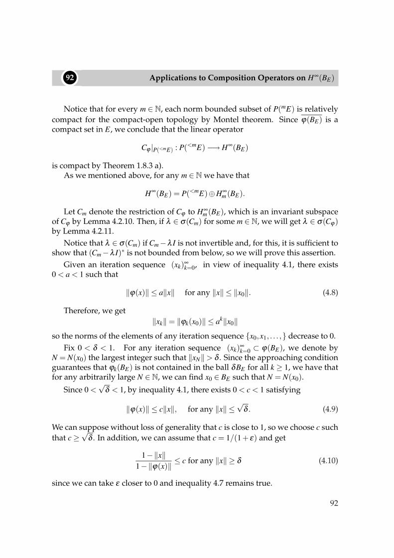
••92 Applications to Composition Operators on H∞(BE)
Notice that for every m ∈ N, each norm bounded subset of P(mE) is relativelycompact for the compact-open topology by Montel theorem. Since ϕ(BE) is acompact set in E, we conclude that the linear operator
Cϕ |P(<mE) : P(<mE)−→ H∞(BE)
is compact by Theorem 1.8.3 a).As we mentioned above, for any m ∈ Nwe have that
H∞(BE) = P(<mE)⊕H∞m (BE).
Let Cm denote the restriction of Cϕ to H∞m (BE), which is an invariant subspace
of Cϕ by Lemma 4.2.10. Then, if λ ∈ σ(Cm) for some m ∈ N, we will get λ ∈ σ(Cϕ)by Lemma 4.2.11.
Notice that λ ∈ σ(Cm) if Cm−λ I is not invertible and, for this, it is sufficient toshow that (Cm−λ I)∗ is not bounded from below, so we will prove this assertion.
Given an iteration sequence (xk)∞k=0, in view of inequality 4.1, there exists
0 < a < 1 such that
‖ϕ(x)‖ ≤ a‖x‖ for any ‖x‖ ≤ ‖x0‖. (4.8)
Therefore, we get‖xk‖= ‖ϕk(x0)‖ ≤ ak‖x0‖
so the norms of the elements of any iteration sequence x0,x1, . . . , decrease to 0.Fix 0 < δ < 1. For any iteration sequence (xk)∞
k=0 ⊂ ϕ(BE), we denote byN = N(x0) the largest integer such that ‖xN‖> δ . Since the approaching conditionguarantees that ϕk(BE) is not contained in the ball δBE for all k ≥ 1, we have thatfor any arbitrarily large N ∈ N, we can find x0 ∈ BE such that N = N(x0).
Since 0 <√
δ < 1, by inequality 4.1, there exists 0 < c < 1 satisfying
‖ϕ(x)‖ ≤ c‖x‖, for any ‖x‖ ≤√
δ . (4.9)
We can suppose without loss of generality that c is close to 1, so we choose c suchthat c≥
√δ . In addition, we can assume that c = 1/(1+ ε) and get
1−‖x‖1−‖ϕ(x)‖ ≤ c for any ‖x‖ ≥ δ (4.10)
since we can take ε closer to 0 and inequality 4.7 remains true.
92
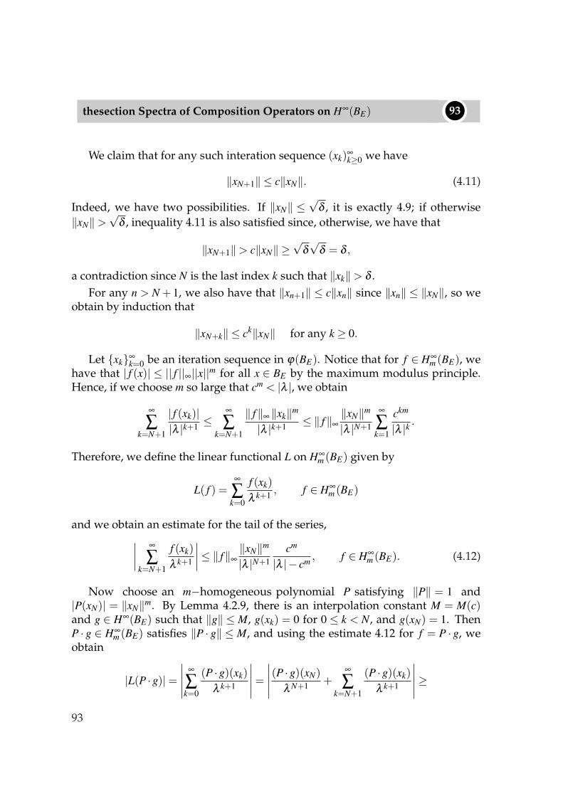
thesection Spectra of Composition Operators on H∞(BE) ••93
We claim that for any such interation sequence (xk)∞k≥0 we have
‖xN+1‖ ≤ c‖xN‖. (4.11)
Indeed, we have two possibilities. If ‖xN‖ ≤√
δ , it is exactly 4.9; if otherwise‖xN‖>
√δ , inequality 4.11 is also satisfied since, otherwise, we have that
‖xN+1‖> c‖xN‖ ≥√
δ√
δ = δ ,
a contradiction since N is the last index k such that ‖xk‖> δ .For any n > N + 1, we also have that ‖xn+1‖ ≤ c‖xn‖ since ‖xn‖ ≤ ‖xN‖, so we
obtain by induction that
‖xN+k‖ ≤ ck‖xN‖ for any k ≥ 0.
Let xk∞k=0 be an iteration sequence in ϕ(BE). Notice that for f ∈ H∞
m (BE), wehave that | f (x)| ≤ || f ||∞||x||m for all x ∈ BE by the maximum modulus principle.Hence, if we choose m so large that cm < |λ |, we obtain
∞
∑k=N+1
| f (xk)||λ |k+1 ≤
∞
∑k=N+1
‖ f‖∞ ‖xk‖m
|λ |k+1 ≤ ‖ f‖∞‖xN‖m
|λ |N+1
∞
∑k=1
ckm
|λ |k .
Therefore, we define the linear functional L on H∞m (BE) given by
L( f ) =∞
∑k=0
f (xk)λ k+1 , f ∈ H∞
m (BE)
and we obtain an estimate for the tail of the series,∣∣∣∣
∞
∑k=N+1
f (xk)λ k+1
∣∣∣∣≤ ‖ f‖∞‖xN‖m
|λ |N+1cm
|λ |− cm , f ∈ H∞m (BE). (4.12)
Now choose an m−homogeneous polynomial P satisfying ‖P‖ = 1 and|P(xN)| = ‖xN‖m. By Lemma 4.2.9, there is an interpolation constant M = M(c)and g ∈ H∞(BE) such that ‖g‖ ≤ M, g(xk) = 0 for 0 ≤ k < N, and g(xN) = 1. ThenP · g ∈ H∞
m (BE) satisfies ‖P · g‖ ≤ M, and using the estimate 4.12 for f = P · g, weobtain
|L(P ·g)|=∣∣∣∣∣
∞
∑k=0
(P ·g)(xk)λ k+1
∣∣∣∣∣ =
∣∣∣∣∣(P ·g)(xN)
λ N+1 +∞
∑k=N+1
(P ·g)(xk)λ k+1
∣∣∣∣∣≥
93

••94 Applications to Composition Operators on H∞(BE)
∣∣∣∣(P ·g)(xN)
λ N+1
∣∣∣∣−∣∣∣∣
∞
∑k=N+1
(P ·g)(xk)λ k+1
∣∣∣∣≥||xN ||m|λ |N+1 −
||xN ||m|λ |N+1
Mcm
|λ |− cm .
SinceMcm
|λ |− cm → 0 when m→ ∞,
we can choose m so that, in addition to cm < |λ |, we have
Mcm
|λ |− cm <12.
Then, since |L(P ·g)| ≤M‖L‖ and ‖xN‖ ≥ δ > 1/4, we get
M‖L‖ ≥ |L(P ·g)| ≥ ‖xN‖m
2|λ |N+1 ≥1
2 ·4m|λ |N+1 . (4.13)
Next observe that for f ∈ H∞m (BE),
((λ I−Cm)∗(L))( f ) = λL( f )−L(Cm( f )) = λL( f )−L( f ϕ) =
λ∞
∑k=0
f (xk)λ k+1 −
∞
∑k=0
f (xk+1)λ k+1 = f (x0).
Hence
‖(λ I−Cm)∗(L)‖ ≤ 1. (4.14)
As we have mentioned above, we can form iteration sequences for which N isarbitrarily large, hence by 4.13 for which ‖L‖ is arbitrarily large. In view of 4.14,we show then that (λ I−Cm)∗ is not bounded below. Consequently (λ I−Cm)∗ isnot invertible, and neither then is λ I−Cm, so that λ ∈ σ(Cm).
4.2.2 A Julia-Type Estimate for C0(X) spaces
In Theorem 4.2.12 we need to assume that a Julia-type estimate for E is satis-fied in order to describe the spectrum of Cϕ . As we recalled in Theorem 4.2.6, thisestimate exists when we deal with Hilbert spaces. In this section we will give aJulia-type estimate for C0(X) spaces, in particular for the n-fold space Cn and c0.
Recall that the pseudohyperbolic distance for A = H∞(BE) with E = C0(X), X alocally compact space, is given by formula 1.8:
94
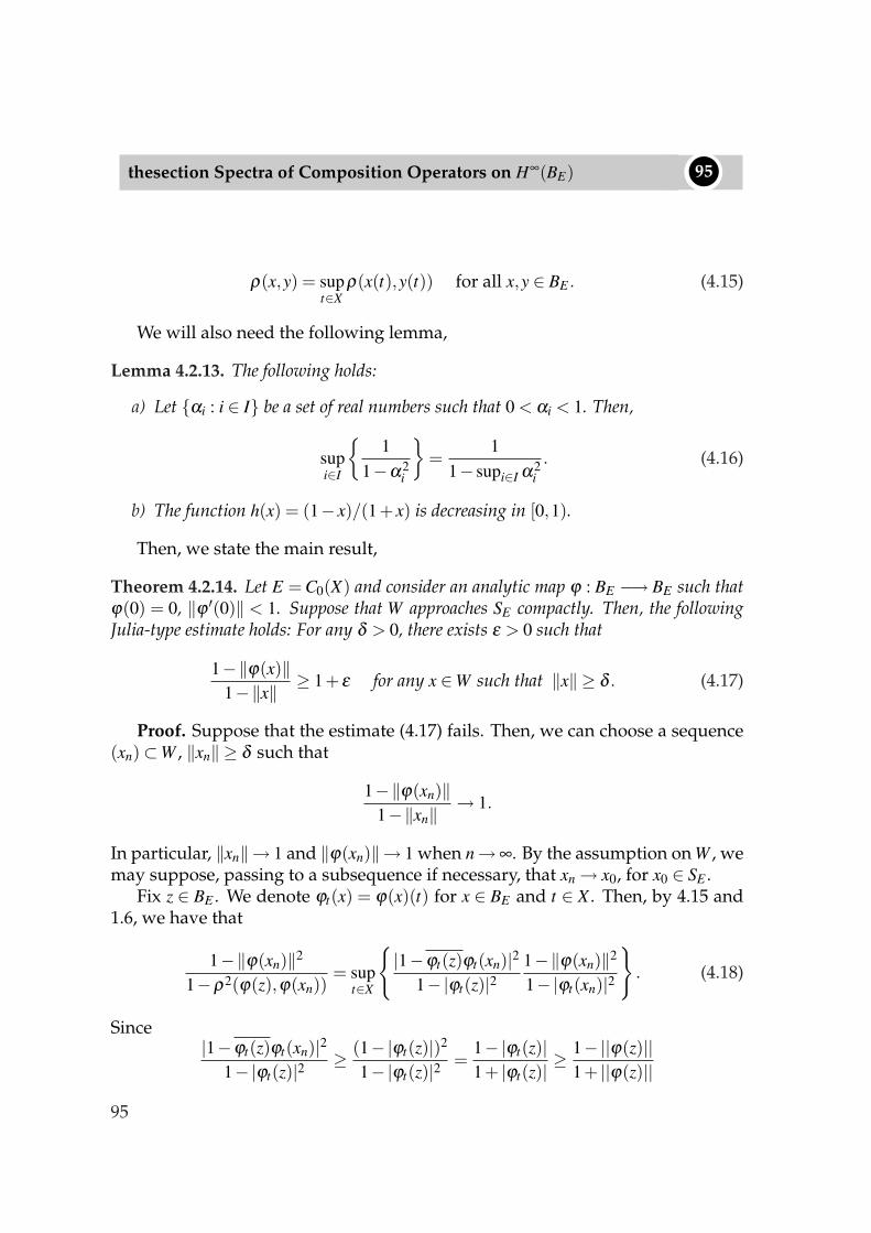
thesection Spectra of Composition Operators on H∞(BE) ••95
ρ(x,y) = supt∈X
ρ(x(t),y(t)) for all x,y ∈ BE . (4.15)
We will also need the following lemma,
Lemma 4.2.13. The following holds:
a) Let αi : i ∈ I be a set of real numbers such that 0 < αi < 1. Then,
supi∈I
1
1−α2i
=
11− supi∈I α2
i. (4.16)
b) The function h(x) = (1− x)/(1+ x) is decreasing in [0,1).
Then, we state the main result,
Theorem 4.2.14. Let E = C0(X) and consider an analytic map ϕ : BE −→ BE such thatϕ(0) = 0, ‖ϕ ′(0)‖ < 1. Suppose that W approaches SE compactly. Then, the followingJulia-type estimate holds: For any δ > 0, there exists ε > 0 such that
1−‖ϕ(x)‖1−‖x‖ ≥ 1+ ε for any x ∈W such that ‖x‖ ≥ δ . (4.17)
Proof. Suppose that the estimate (4.17) fails. Then, we can choose a sequence(xn)⊂W , ‖xn‖ ≥ δ such that
1−‖ϕ(xn)‖1−‖xn‖ → 1.
In particular, ‖xn‖→ 1 and ‖ϕ(xn)‖→ 1 when n→∞. By the assumption on W , wemay suppose, passing to a subsequence if necessary, that xn → x0, for x0 ∈ SE .
Fix z ∈ BE . We denote ϕt(x) = ϕ(x)(t) for x ∈ BE and t ∈ X . Then, by 4.15 and1.6, we have that
1−‖ϕ(xn)‖2
1−ρ2(ϕ(z),ϕ(xn))= sup
t∈X
|1−ϕt(z)ϕt(xn)|2
1−|ϕt(z)|21−‖ϕ(xn)‖2
1−|ϕt(xn)|2
. (4.18)
Since|1−ϕt(z)ϕt(xn)|2
1−|ϕt(z)|2 ≥ (1−|ϕt(z)|)2
1−|ϕt(z)|2 =1−|ϕt(z)|1+ |ϕt(z)| ≥
1−||ϕ(z)||1+ ||ϕ(z)||
95
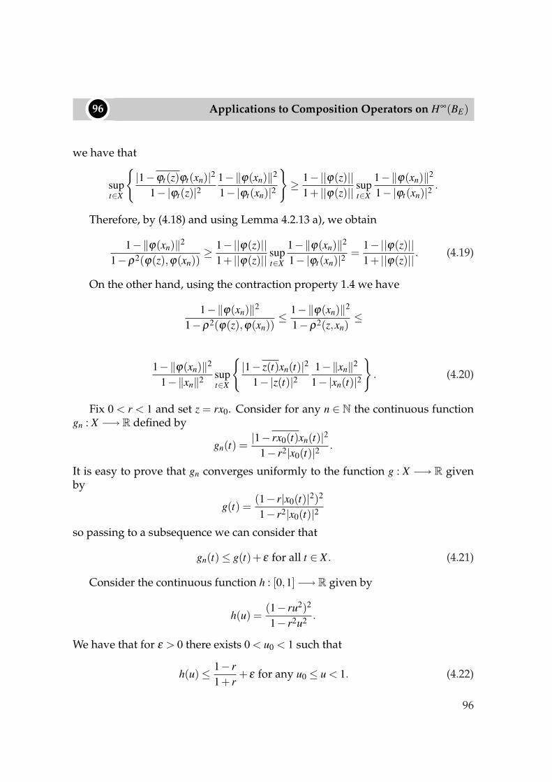
••96 Applications to Composition Operators on H∞(BE)
we have that
supt∈X
|1−ϕt(z)ϕt(xn)|2
1−|ϕt(z)|21−‖ϕ(xn)‖2
1−|ϕt(xn)|2≥ 1−||ϕ(z)||
1+ ||ϕ(z)|| supt∈X
1−‖ϕ(xn)‖2
1−|ϕt(xn)|2 .
Therefore, by (4.18) and using Lemma 4.2.13 a), we obtain
1−‖ϕ(xn)‖2
1−ρ2(ϕ(z),ϕ(xn))≥ 1−||ϕ(z)||
1+ ||ϕ(z)|| supt∈X
1−‖ϕ(xn)‖2
1−|ϕt(xn)|2 =1−||ϕ(z)||1+ ||ϕ(z)|| . (4.19)
On the other hand, using the contraction property 1.4 we have
1−‖ϕ(xn)‖2
1−ρ2(ϕ(z),ϕ(xn))≤ 1−‖ϕ(xn)‖2
1−ρ2(z,xn)≤
1−‖ϕ(xn)‖2
1−‖xn‖2 supt∈X
|1− z(t)xn(t)|2
1−|z(t)|21−‖xn‖2
1−|xn(t)|2
. (4.20)
Fix 0 < r < 1 and set z = rx0. Consider for any n ∈ N the continuous functiongn : X −→ R defined by
gn(t) =|1− rx0(t)xn(t)|2
1− r2|x0(t)|2 .
It is easy to prove that gn converges uniformly to the function g : X −→ R givenby
g(t) =(1− r|x0(t)|2)2
1− r2|x0(t)|2so passing to a subsequence we can consider that
gn(t)≤ g(t)+ ε for all t ∈ X . (4.21)
Consider the continuous function h : [0,1]−→ R given by
h(u) =(1− ru2)2
1− r2u2 .
We have that for ε > 0 there exists 0 < u0 < 1 such that
h(u)≤ 1− r1+ r
+ ε for any u0 ≤ u < 1. (4.22)
96
thesection Spectra of Composition Operators on H∞(BE) ••97
Therefore, by (4.21) and (4.22) we have
gn(t)≤ 1− r1+ r
+2ε for any |x0(t)| ≥ u0.
Consider the supremum from inequality (4.20) and pay attention to items with|x0(t)|< u0. We have
|1− x0(t)xn(t)|21− r2|x0(t)|2
1−‖xn‖2
1−|xn(t)|2 ≤|1− rx0(t)xn(t)|2
1− r2|x0(t)|21−‖xn‖2
1−u20
≤ 4(1−‖xn‖2)(1−u2
0)(1− r2).
On the other hand, if we pay attention to items with |x0(t)| ≥ u0 we obtain that
1−‖ϕ(xn)‖2
1−ρ2(ϕ(rx0),ϕ(xn))≤ (4.23)
1−‖ϕ(xn)‖2
1−‖xn‖2 sup|x0(t)|≥u0
|1− rx0(t)xn(t)|2
1−|rx0(t)|21−‖xn‖2
1−|xn(t)|2 ,4(1−‖xn‖2)
(1−u20)(1− r2)
≤
1−‖ϕ(xn)‖2
1−‖xn‖2 max|x0(t)|≥u0
|1− rx0(t)xn(t)|2
1−|rx0(t)|2 ,4(1−‖xn‖2)
(1−u20)(1− r2)
.
If we let n→ ∞ in the last term, we obtain
limsupn→∞
1−‖ϕ(xn)‖2
1−ρ2(ϕ(rx0),ϕ(xn))≤ (1− r)
1+ r+2ε. (4.24)
Consequently, by (4.19) and (4.24), we obtain
(1− r)1+ r
+2ε ≥ 1−||ϕ(rx0)||1+ ||ϕ(rx0)||
and hence, if ε tends to 0, we obtain that ||ϕ(rx0)|| ≥ r = ||rx0||, a contradiction.
By Theorems 4.2.12 and 4.2.14, we obtain an extension of Theorem 4.2.2 fornon power compact composition operators Cϕ .
Theorem 4.2.15. Let E be a C0(X) space and consider an analytic map ϕ : BE −→ BEsuch that ϕ(0) = 0, ‖ϕ ′(0)‖< 1 and ϕ(BE) is relatively compact in BE . Suppose that ϕsatisfies the approaching condition. Then, σ(Cϕ) = D.
97
••98 Applications to Composition Operators on H∞(BE)
Proof. Apply Theorem 4.2.14 to W = ϕ(BE), which approaches SE compactlysince ϕ(BE) is relatively compact and does not lie inside BE . Then, we find theJulia-type estimate necessary to apply Theorem 4.2.12 and conclude the result.
In particular, the result is valid for c0 and we obtain the following corollaryfor the n-fold space Cn,
Corollary 4.2.16. Let ϕ : Dn −→ Dn an analytic map such that ϕ(0) = 0 and‖ϕ ′(0)‖< 1. If Cϕ : H∞(Dn)−→ H∞(Dn) is non-power compact, then σ(Cϕ) = D.
4.3 Radon-Nikodým Composition Operators
In this section we aim to study Radon-Nikodým composition operators. Inorder to do it we use the Asplund sets. The notion of Asplund set in a Banachspace E arises in studying differentiability properties of the norm of E. At sametime, there exists a strong duality between the Asplund property and the Radon-Nikodým property on Banach spaces. Further references can be found in [Asp68],[Ste81], [Fit80] and [Bgi83].
We begin with some background on the Radon-Nikodým property.
4.3.1 Background on the Radon-Nikodým Property
In order to introduce the class of Radon-Nikodým operators, we will givesome background on the Radon-Nikodým property for Banach spaces. For fur-ther results, see [Saa80], [Ste81] and [DU77].
A measurable space is a pair (Ω,Σ), such that Ω is a set and Σ a σ -algebra ofsubsets of Ω. The triple (Ω,Σ,µ) is a measure space if (Ω,Σ) is a measurable spaceand µ is a finite nonnegative measure on Σ. All the measures treated are count-ably additive unless the contrary is explicitly stated. The classical Radon-NikodýmTheorem states as follows:
Theorem 4.3.1 (Radon-Nikodým). Let (Ω,Σ,µ) a finite measure space and m : Σ→Ra finite measure which is absolutely continuous with respect to µ (m << µ). Then, thereexists a µ-integrable function f : Ω−→ R, denoted by dm/dµ , such that
∫
Af dµ = m(A) for any A ∈ Σ.
98
thesection Radon-Nikodým Composition Operators ••99
In order to replace R by a general Banach space E in both instances above, werecall the following:
Let Σ be a σ−algebra and E a Banach space. A map m : Σ −→ E such thatm( /0) = 0 ∈ X is called a vector measure (or an E-valued measure) if it is countablyadditive; that is, whenever
A j
∞j=1 is a sequence of pairwise disjoint sets in E,
then
m(∪∞j=1A j) =
∞
∑j=1
m(A j).
Such a measure is said to be absolutely continuous with respect to µ (m << µ) if forA ∈ Σ, the condition µ(A) = 0 implies m(A) = 0.
Now we give the concept of Bochner integrability, which generalizes measuretheory to vector measures.
Denote by χA the characteristic function of a subset A⊂E. A function s : Ω→Eis called a simple function if s can be written in the form ∑n
i=1 xiχAi for distinct xi ∈E,i = 1, . . . ,n and a finite partition Ain
i=1 of Ω chosen from Σ.
Definition 4.3.2. A function f : Ω−→E is said to be µ-Bochner integrable if there existsa sequence (sn) of simple functions such that
i) limn sn(ω) = f (ω) µ−a.e.ii) limn
∫Ω ‖ f (ω)− sn(ω)‖dµ(ω) = 0.
The set of Bochner integrable functions is denoted by L1X(Ω,Σ,µ) or simply
L1X(µ). When f is Bochner integrable, the limit limn
∫A sndµ exists independently
of the particular choice of (sn) and the integral is defined by∫
Af dµ = lim
n
∫
Asn dµ.
Definition 4.3.3. A closed, bounded, convex subset C of a Banach space E is called aRadon-Nikodým set if, for any probability space (Ω,Σ,P) and any E-valued vectormeasure m : Σ−→ E such that the average of m is in C (i.e. m(A)/P(A) is in C for everyA ∈ Σ), there exists a P-Bochner integrable function f : Ω−→ E such that
m(A) =∫
Af dP for all A ∈ Σ.
A Banach space E is said to have the Radon-Nikodým property if each E-valuedmeasure on Σ which is of finite total variation and satisfies m << µ , admits anf ∈ L1
X(Ω,Σ,µ) such that∫
Af dµ = m(A) for each A ∈ Σ.
99
••100 Applications to Composition Operators on H∞(BE)
The concept of Radon-Nikodým operator is the following [GS84],
Definition 4.3.4. The linear operator T : E −→ F is said to be a Radon-Nikodýmoperator if for every finite measure space (Ω,Σ,λ ) and for every vector measureG : Σ −→ E such that ‖G(B)‖ ≤ λ (B) for all B ∈ Σ, there exists a Bochner integrablefunction f : Ω−→ F such that
T G(B) =∫
Bf dλ for all B ∈ Σ.
It is well-known that E has the Radon-Nikodým property if and only if IE is aRadon-Nikodým operator [Bgi83].
It is also well-known [Pie80] that the set of Radon-Nikodým operators is aclosed ideal of operators. In connection with Radon-Nikodým operators, thestrong Radon-Nikodým operators are defined as follows,
Definition 4.3.5. We say that T : E −→ F is a strong Radon-Nikodým operator ifT (BE) is a Radon-Nikodým set.
If T : E −→F is a strong Radon-Nikodým operator, then T is a Radon-Nikodýmoperator by [Edg80]. The converse is not true since any quotient Q from `1 ontoc0 is a Radon-Nikodým operator but is not a strong Radon-Nikodým operator[GS84]. Nevertheless, it follows from [Ste81] the following result which statesthat these concepts are equivalent for adjoint maps,
Theorem 4.3.6. Let T : E −→ F be a bounded linear operator. Then T ∗ : F∗ −→ E∗ is astrong Radon-Nikodým operator if and only if it is a Radon-Nikodým operator.
4.3.2 Asplund sets
This section is devoted to the study of the Asplund property. We will givesome background on Asplund sets and operators and will study some relatedproperties. Then, we will give conditions for polynomials between Banach spacesto preserve the Asplund property of some sets and will derive some consequences.
We recall the definition of S. Fitzpatrick [Fit80] of Asplund set. He showed thatthis definition is equivalent to the earlier one related to the differentiability of thenorm of E. Recall that, given a subset A⊂ E, the seminorm ‖ · ‖A : E∗ −→ [0,∞) ofE∗ is given by
‖ f‖A = supx∈A
| f (x)|.
100
thesection Radon-Nikodým Composition Operators ••101
Definition 4.3.7. Let E be a Banach space and A ⊂ E. A bounded set D ⊂ E is said tobe an Asplund set if, for any countable set A ⊂ D, the seminormed space (E∗,‖ · ‖A) isseparable. The space E is said to be an Asplund space if its unit ball BE is an Asplundset.
Proposition 4.3.8. Let D⊂ E. Then, D is an Asplund set if and only if the closure of itsabsolutely convex hull Γ(D) is an Asplund set.
There are many characterizations of Asplund spaces [Bgi83]. The followingone will be used later,
Proposition 4.3.9. The Banach space E is Asplund if and only if, for any separablesubspace F ⊂ E, we have that F∗ es separable.
By 4.3.9, it is clear that any reflexive Banach space is an Asplund space. Fur-thermore, if E∗ is separable, then E is also an Asplund space. In addition, wehave the following proposition:
Proposition 4.3.10. Let T : E −→ F a linear operator and D⊂ E a bounded set. If D isan Asplund set, then T (D) is an Asplund set as well.
We wonder if it is possible to extend Proposition 4.3.10 to nonlinear mappings.In particular, we are interested in studying analytic maps from E to F . The fol-lowing example shows that this extension cannot be done in general.
Example 4.3.11. Set E = `2 and F = `1. Consider the polynomial P ∈ P(2`2, `1) givenby
P((xn)∞n=1) = (x2
n)∞n=1.
Then P does not transform Aslpund sets into Asplund sets.
To show this, consider the set D = en : n ∈ N, which is is an Asplund set in `2.However, P(D) = D is not an Asplund set in `1; indeed, `∗1 = `∞ and the space(`∞,‖ · ‖D) is not separable since for f = ( fn) ∈ `∞ we have
‖ f‖D = supx∈D
| f (x)|= supn∈N
| fn|= ‖ f‖∞
so ‖ · ‖D is the usual norm for `∞ and, therefore, (`∞,‖ · ‖D) is not separable.
Therefore, we aim to find sufficient conditions for analytic mappings to trans-form Asplund sets into Asplund sets. This will lead us to characterize Radon-Nikodým composition operators Cϕ in terms of ϕ(BE). The following lemma (see[Bgi83]) will be needed,
101

••102 Applications to Composition Operators on H∞(BE)
Lemma 4.3.12. Let E be a Banach space. Then,a) The sum and the union of a finite number of Asplund sets in E is an Asplund set.b) Let (Dn) be a sequence of Asplund sets in E and let (tn) be a sequence of positive
numbers such that limn tn = 0. Then, the set
D =∞⋂
n=1
(Dn + tnBE)
is an Asplund set.
Let U be a subset of E. A subset D⊂U is said to be U-bounded if D is boundedand d(D,ErU) > 0. A function f : U −→ F is said to be of bounded type if it mapsU-bounded sets into bounded sets.
Proposition 4.3.13. Let E and F be Banach spaces and D⊂ E an Asplund set.
a) Suppose that P(kE) = Pf (kE) for some k ∈ N. If P : E −→ F is a k-homogeneouspolynomial, then P(D) is an Asplund set.
b) Suppose that P(kE) = Pf (kE) for any k∈N. If f : U ⊂E −→F is an analytic functionof bounded type and D is U- bounded, then f (D) is an Asplund set.
Proof. We can suppose, without loss of generality, that D⊂ BE , since the classof Asplund sets is stable under translations and homotheties.a) Set A ⊂ P(D) a countable set, that is, A = P(C) for some countable set C ⊂ D.Since D is Asplund, we have that (E∗,‖ · ‖C) is separable, so there exists acountable set S which is dense in (E∗,‖ · ‖C). Consider the adjoint mappingP∗ : F∗ −→ P(kE) given by
P∗(ϕ) = ϕ P.
Clearly, the mapping P∗ : (F∗,‖ · ‖A) −→ (P(kE),‖ · ‖C) is a linear isometry.Therefore, (F∗,‖ · ‖A) is separable if P∗(F∗) ⊂ (P(kE),‖ · ‖C) is separable and thiswill be a consequence of the separability of the seminormed space (P(kE),‖ · ‖C).This space is separable since the algebra generated by S is dense in (Pf (kE),‖ ·‖C),which is, again, dense in (P(kE),‖ · ‖C) since Pf (kE) = P(kE) by assumption andthe norm topology is finer than the ‖ · ‖C - topology.
b) By 4.3.12 a) and a) in this Proposition, any polynomial defined on E mapsD into an Asplund set. Set n ∈ N. Since f is of bounded type, there exists apolynomial Pn such that ‖ f (x)−Pn(x)‖ ≤ 1/n for any x ∈ D. Therefore,
f (D)⊂ Pn(D)+1n
BF ,
102
thesection Radon-Nikodým Composition Operators ••103
and, hence, f (D) is an Asplund set by 4.3.12 b).
The following example shows that the G∞(BE), the predual of H∞(BE) definedin paragraph 1.6.5 is not an Asplund space regardless of the Banach space E.
Example 4.3.14. The space G∞(BE) is not Asplund.
Indeed, we know that c0 ⊂ H∞(BE) by Theorem 1.3.4 and, then, `1 ⊂ G∞(BE) byTheorem 4 in [BP58]. Therefore, G∞(BE) has not the Asplund property by Propo-sition 4.3.9 since `∗1 = `∞ is not separable.
This remark leads us to show that Proposition 4.3.13 b) does not hold for nonU-bounded sets. To show this, consider the map δ : D→G∞ given by δ (x) = δx, theevaluation at x. Then δ (D) = δx : x ∈ D is not an Asplund set since the closureof its absolutely convex hull is BG∞ by Proposition 1.3.
The following result gives a sufficient condition for all functions in the alge-bra Au(BE ,F) to transform Asplund sets into Asplund sets. This result can beextended to other algebras of analytic functions on BE .
Proposition 4.3.15. Let E and F be complex Banach spaces and suppose that Au(BE) isseparable. Then, any f ∈ Au(BE ,F) transforms Asplund sets into Asplund sets.
Proof. We denote by A the algebra Au(BE ,F). Pick f ∈ A and consider the re-striction f ∗ :=C f |F∗ : F∗−→Au(BE) given by f ∗(y∗)(x) = y∗( f (x)) for any x∈E. LetD⊂ BE be an Asplund set. To show that f (D)⊂ F is also an Asplund set, considerthe space (F∗,‖ · ‖ f (D)) and B ⊂ f (D) a countable set. There exists a countableset C ⊂ D such that f (C) = B. In consequence, (Au(BE),‖ · ‖C) is separable since‖g−h‖C ≤ ‖g−h‖∞ for any g,h ∈ Au(BE). Since f ∗ : (F∗,‖ · ‖ f (D))→ (Au(BE),‖ · ‖D)is a linear isometry, we have that (F∗,‖ · ‖ f (C)) is separable and, therefore, f (D) isan Asplund set.
Remark 4.3.16. We have the following results,(i) There exist Banach spaces E such that E∗ is separable, so E is Asplund, but there exist
functions f ∈ Au(BE ,F) which do not transform Asplund sets into Asplund sets.To show this, it is sufficient to consider Example 4.3.11.
(ii) There exist Banach spaces E whose dual spaces E∗ are not separable but anyf ∈ Au(BE ,F) transforms Asplund sets into Asplund sets for any Banach space F .Consider, for instance, E = c0(Γ) for Γ an uncountable set, whose dual space `1(Γ)is not separable. However, any function f ∈ Au(BE ,F) transforms Asplund setsinto Asplund sets by Proposition 4.3.13 b).
103
••104 Applications to Composition Operators on H∞(BE)
4.3.3 Radon-Nikodým Composition Operators
Now we recall the duality between the Radon-Nikodým property and the As-plund property. Then, we will give some conditions for composition operators tobe Radon-Nikodým operators.
Definition 4.3.17. The linear operator T : E −→ F is said to be an Asplund operatorif T (BE) is an Asplund set.
The following result can be found in [Bgi83],
Theorem 4.3.18. Let T : E −→ F be a linear operator. Then,T is Asplund if and only if T ∗ is (strong) Radon-Nikodým.
Notice that condition on strongness on T ∗ can be removed since, as we men-tioned in the background, an adjoint operator T ∗ is strong Radon-Nikodým if andonly if it is Radon-Nikodým.
In the following corollary we apply this theorem to Cϕ : H∞(BF) −→ H∞(BE).It is easy that the range of C∗ϕ |G∞(BE) is contained in G∞(BF) since for anyu ∈G∞(BE), the composition uCϕ is still τc-continuous on BG∞(BF ). We denote byCϕ the restriction Cϕ
∗|G∞(BE). Since (Cϕ)∗ = (Cϕ∗|G∞(BE))∗ = Cϕ , we obtain
Corollary 4.3.19. A composition operator Cϕ : H∞(BF)−→H∞(BE) is Radon-Nikodýmif and only if the operator Cϕ : G∞(BE)−→ G∞(BF) is Asplund.
The following result makes it easier the study of the Asplundness of the oper-ator Cϕ .
Proposition 4.3.20. The operator Cϕ is Asplund if and only if the set
δϕ(x) : x ∈ BE
is Asplund in G∞(BF).
Proof. Set B = BG∞(BE). The set Cϕ∗(B) =
µ Cϕ : µ ∈ B
is Asplund if and
only if Γ(
δx Cϕ : x ∈ BE) is Asplund if and only if
δx Cϕ : x ∈ BE
is Asplund
if and only if
δϕ(x) : x ∈ BE
is Asplund.
Notice that Example 4.3.14 shows that
δϕ(x) : x ∈ BE
being an Asplund set isnot equivalent to ϕ(BE) being an Asplund set.
In the following result, we apply Proposition 4.1.1.
Proposition 4.3.21. Let Cϕ : H∞(BF)−→H∞(BE) be a Radon-Nikodým operator. Then,there exists 0 < r < 1 such that ϕ(BE)⊂ rBF .
104
thesection Radon-Nikodým Composition Operators ••105
Proof. If such an 0 < r < 1 does not exist, we apply Proposition 4.1.1 and findlinear operators T : `∞ −→H∞(BE) and S : H∞(BE)−→ `∞ such that SCϕ T = Id`∞ .This is not possible since the class of Radon-Nikodým operators is an operatorideal and Id`∞ is not Radon-Nikodým.
Now we present a characterization of Radon-Nikodým composition opera-tors in terms of the Asplund property and the condition given in the previousproposition.
Theorem 4.3.22. The composition operator Cϕ : H∞(BF)−→H∞(BE) is Radon-Nikodýmif and only if there exists 0 < r < 1 such that ϕ(BE)⊂ rBF and (P(F),‖ ·‖A) is separablefor any countable set A⊂ ϕ(BE).
Proof. To prove the sufficient condition it is enough to show that δϕ(BE) =δx : x ∈ ϕ(BE) is an Asplund set in G∞(BF) by Proposition 4.3.20 and Corollary4.3.19. Let 0 < r < 1 such that ϕ(BE) ⊂ rBF . Let A ⊂ ϕ(BE) a countable set. Thisset can be described as A = ϕ(C) for some countable set C ⊂ BE . Recall that theTaylor series of f ∈ H∞(BF) converge uniformly to f on rBF and, therefore, f isuniformly approximable by polynomials on ϕ(C). In consequence, P(F) is densein (H∞(BF),‖ · ‖ϕ(C)). Since (P(F),‖ · ‖ϕ(C)) is separable and (G∞(BF))∗ = H∞(BF) ,it follows that ((G∞(BF))∗,‖ · ‖ϕ(C)) is separable. Then, δϕ(BE) is an Asplund set inG∞(BF) and Cϕ is Radon-Nikodým.
Now we prove the necessary conditions. Let Cϕ Radon-Nikodým. Then, byProposition 4.3.21, there exists 0 < r < 1 such that ϕ(BE)⊂ rBF . To show the othercondition, let A ⊂ ϕ(BE) a countable set, that is, A = ϕ(C) for some countable setC ⊂ BE . Since Cϕ(BG∞(BE)) is an Asplund set, the space (H∞(BF),‖ · ‖ϕ(C)) is sepa-rable. Therefore, since P(F)⊂H∞(BF), it follows that (P(F),‖·‖ϕ(C)) is a subspaceof the seminormed space (H∞(BF),‖ · ‖ϕ(C)). Then, (P(F),‖ · ‖A) is separable.
Corollary 4.3.23. Let ϕ : BE −→ BF be an analytic map.
a) Suppose that P(kF) = Pf (kF) for any k ∈ N. If ϕ(BE) is an Asplund set andthere exists 0 < r < 1 such that ϕ(BE) ⊂ rBF , then the composition operatorCϕ : H∞(BF)−→ H∞(BE) is Radon-Nikodým.
b) Suppose that the algebra Au(BF) is separable. If ϕ(BE) is an Asplund set andthere exists 0 < r < 1 such that ϕ(BE) ⊂ rBF , then the composition operatorCϕ : H∞(BF)−→ H∞(BE) is Radon-Nikodým.
Proof. a) In Proposition 4.3.13 a), we show that for any countable setC ⊂ ϕ(BE), the space (P(kF),‖ · ‖C) is separable. Then,
(P(F),‖ · ‖C) =⋃
k∈N(P(kF),‖ · ‖C)
105
••106 Applications to Composition Operators on H∞(BE)
is also separable and, therefore, we can use the previous theorem to get the result.
b) Since ϕ(BE) ⊂ rBF is an Asplund set and the function δ |rBF belongs toAu(rBF ,G∞(BF)), we have, if Au(BF) is separable, that the set δϕ(BE) is also anAsplund set by Corollary 4.3.15 and, therefore, the composition operator Cϕ isRadon-Nikodým.
106
Ch
ap
ter 5 Hankel-type OperatorsHankel-type Operators
Hankel operators were first studied acting on the Hardy space H2 and theywere extended to act on closed subspaces of C(K) spaces, in particular, on uni-form algebras. Several properties of these subspaces can be described throughthese operators, which will be called Hankel-type operators. Their weak com-pactness and their compactness led to introduce the concept of tightness of a uni-form algebra. The complete continuity of the Hankel operators led to define theso-called Bourgain algebras, which are closely related to the Dunford-Pettis prop-erty.
5.1 Background
Let us introduce some basic results and notation related to Hankel operators.For further results, see [Pow82], [Zhu90] and [Pel98].
5.1.1 The Hankel-type operators
Let H2 denote the usual Hardy space of functions on the circle ∂D and considerthe Cauchy projection C from L2 onto H2 defined in paragraph 1.4.1. The classicalHankel operators correspond to functions g ∈ L2 which act on H2 by definingSg : H2 −→ (H2)⊥ by
S f (g) = g f −C (g f ).
The aim of the Hankel-type operators is the extension of Hankel operators toclosed subspaces of C(K), in particular, to uniform algebras. Since such operatorsare multiplication operators into the orthogonal, the most natural candidate is toconsider the following definition found in [CG82],
107
••108 Hankel-type Operators
Definition 5.1.1. Let A be a uniform algebra on K and g ∈ C(K). The Hankel-typeoperator Sg : A−→C(K)/A is defined according to
Sg( f ) = g f +A.
It is obvious that Hankel-type operators are linear. They are also continuoussince
‖Sg( f )‖= ‖g f +A‖= inf‖g f + x‖∞ : x ∈ A ≤ ‖g f‖∞ ≤ ‖g‖∞‖ f‖∞.
When we deal with closed operator ideals U , we define the sets
AU =
g ∈C(K) : Sg ∈U
and AU ∗∗ =
g ∈C(K) : S∗∗g ∈U
.
We have the following result,
Proposition 5.1.2. Let U be a closed operator ideal. Then, AU and AU ∗∗ are closedsubspaces of C(K).
Proof. It is easy to show that AU and AU ∗∗ are subspaces of C(K). Then,we prove that AU is closed. Recall that Sg is continuous and ‖Sg‖ ≤ ‖g‖∞. Letgn a sequence of functions of AU converging to g0 ∈ C(K). By the inequality‖Sg‖ ≤ ‖g‖∞ we deduce that Sgn converges to Sg0 and, since U is a closed operatorideal, we obtain that Sg0 ∈U . As consequence, g0 ∈ AU and therefore the set is aclosed subspace.
Examples of closed operator ideals are the class of compact and weakly com-pact operators and the class of completely continuous operators. When we dealwith these classes of operators, the sets AU and AU ∗∗ are, indeed, closed subalge-bras of C(K) as we will recall later.
5.1.2 The Dunford-Pettis property and Bourgain Algebras
The birthplace of the Dunford-Pettis property is a work of A. Grothendieck[Gro53] where he proved that weakly compact operators T : C(K)−→ F are com-pletely continuous for any Banach space F . This was an extension of the workdone by N. Dunford and B. J. Pettis in [DP40] for weakly compact operators onL1(µ).
Definition 5.1.3. A Banach space E is said to have the Dunford-Pettis property (DPproperty) if any weakly compact operator T : E −→ F is completely continuous for anyBanach space F .
108
thesection Background ••109
It is well-known [Die80] that E has the DP property if and only iflimn x∗n(xn) = 0 for sequences xn
w→ 0 in E and x∗nw→ 0 in E∗. Then, it is clear that E
has the DPP if E∗ also enjoys it. The reciprocal is false in general, as was shownby C. Stegall [Ste72]. The DP property is hereditary for complemented subspacesbut not for closed subspaces in general [PS65]. It is also well-known that there areno reflexive infinite dimensional Banach spaces satisfying the DP property. Forfurther results about the DP property, see [Die80].
If we deal with algebras of analytic functions, we find several results relatedto the DP property; J. Chaumat [Cha74] proved that the disk algebra A(D) hasthe DP property and J. Bourgain proved it for H∞ [Bou84b], the ball algebrasA(Bn) and the polydisk algebras A(Dn) [Bou84a]. We recall the main results of theBourgain’s work in [Bou84a], which will be connected to our results on Bourgainalgebras given in section 5.2. The main theorem in [Bou84a] allows to prove thatA(Bn) and A(Dn) enjoy the DP property:
Theorem 5.1.4. Let E be the ball algebra A(Bn) or the polydisk algebra A(Dn). Then, anybounded sequence (x∗n) in E∗ either tends uniformly to zero on weakly compact subsets ofE∗∗ or c0 ⊂ E and (x∗n) does not tend uniformly to zero on the c0-basis (ek).
Besides,
Proposition 5.1.5. If E satisfies the thesis of Theorem 5.1.4, then E∗, and hence E, havethe DP property.
To prove Theorem 5.1.4, J. Bourgain develops a procedure to obtain c0−se-quences. Recall that the product defined in C(K)∗∗ is given by the Arens product(see paragraph 1.3.2). We denote by (ek) the canonical basis of c0 or an isomorphicspace to c0. Bourgain’s result states as follows,
Theorem 5.1.6. Let E be a closed subspace of C(K), (x∗n) a bounded sequence in E∗ andδ > 0. Suppose that the following property holds,
(P) For each g ∈C(K) and each ε > 0, there exists a sequence (x∗∗n ) ⊂ BE∗∗ which isweakly convergent to 0 such that
i) limsupn |x∗∗n (x∗n)|> δii) d(g · x∗∗n ,E∗∗) < ε for any n ∈ N.
Then, c0 ⊂ E and supn |x∗n(ek)|> δ/2.
Theorem 5.1.6 led him to prove that the ball algebras A(Bn) satisfy Theorem5.1.4, and hence the Dunford-Pettis property. Recall that the spectrum of the ballalgebra A(Bn) is given by Bn. J. Bourgain’s way to Theorem 5.1.6 was opened by
109

••110 Hankel-type Operators
Proposition 5.1.7. Let A be the ball algebra A(Bn). Then, for any x∗∗nw→ 0 in A∗∗ and
g ∈C(Bn), we have that limn→∞ d(g · x∗∗n ,A) = 0.
Proposition 5.1.7 proves that property (P) in Theorem 5.1.6 is satisfied whenwe deal with A(Bn) and, hence, Theorem 5.1.4 as mentioned above. We obtainthat A(Bn) and A(Bn)∗ enjoy the DP property.
J. A. Cima and R. M. Timoney [CT87] studied the Bourgain’s work and founda convenient reformulation of his results. They introduced the so-called Bour-gain algebras, which are closely connected to Theorem 5.1.6 and Proposition 5.1.7.Such sets contain the symbols of Hankel-type operators on the algebra whichare completely continuous. This will give a connection between tightness, theDunford-Pettis property and the Bourgain algebras.
Definition 5.1.8. Let X be a closed subspace of C(K). Then, the sets defined by
Xb =
g ∈C(K) : Sg : X −→C(K)/A is completely continuous
and
XB =
g ∈C(K) : S∗∗g : X∗∗ −→C(K)∗∗/A∗∗ is completely continuous
.
are closed subalgebras of C(K) and are called the Bourgain algebras of X .
We will refer to Xb as the big Bourgain algebra and XB as the small Bourgainalgebra. In addition, we have the following result [CT87],
Proposition 5.1.9. Let A be a closed subalgebra of C(K). Then, its Bourgain algebras Aband AB satisfy A⊂ AB ⊂ Ab.
The J. A. Cima and R. M. Timoney reformulation can be summarized as fol-lows,
Theorem 5.1.10. Let X be a closed subspace of C(K). Then,i) If Xb = C(K) then X has the DPP.
ii) If XB = C(K) then both X∗ and X have the DPP.
Theorem 5.1.11. Let A be the ball algebra A(Bn) on K = Bn. Then, its Bourgain algebrasAb and AB are both equal to C(K). Hence, A∗ and A have the DP property.
A proof by induction using Theorem 5.1.4 allowed J. Bourgain to concludethat A(Dn) and its dual also enjoy the DP property. Nevertheless, the line of theproof is different to the one used for A(Bn) because it was not clear whether theBourgain algebras of A(Dn) were the whole C(K) or not.
110
thesection The Bourgain algebras of A(Dn) ••111
5.1.3 Tightness
The concept of tightness was introduced by B. J. Cole and T.W. Gamelin in[CG82]. It is related to Hankel-type operators on uniform algebras and reads asfollows,
Definition 5.1.12. Let K be a compact space. A closed subspace X of C(K) is said to betight if the Hankel-type operator Sg is weakly compact for any g ∈C(K).
S. F. Saccone introduced a concept related to tightness in [Sac97]:
Definition 5.1.13. A closed subspace X of C(K) is said to be strongly tight if for anyg ∈C(K), the Hankel-type operator Sg is compact.
It is clear that a strongly tight subspace is also tight. Saccone also observedthat infinite-dimensional reflexive spaces are tight in any C(K) space they areembedded in, but can never be realized as strongly tight subspaces. However,there is no known example of a tight uniform algebra which fails to be stronglytight. If X is strongly tight, then X∗, hence X enjoy the DP property by Theorem5.1.10. S. F. Saccone also proved that X enjoys the Pelczynski property (V) and itsdual is weakly sequentially complete if X is tight.
The space A∗∗ +C(K) is always a closed subspace of C(K)∗∗. In [CG82] it isproved that A is tight if and only if A∗∗+C(K) is a closed subalgebra of C(K)∗∗.In addition, this property is, roughly speaking, the abstract analogue of the solv-ability of a certain abstract ∂ -problem with a small gain in smoothness.
B. J. Cole and T. W. Gamelin proved that A(Dn) is not tight for n ≥ 2. How-ever, they proved that the algebra A(D) is tight when D is a strictly pseudoconvexdomain in Cn for which a certain ∂ -problem is appropriately solvable. Further re-sults on tightness of the algebra generated by the weak∗-continuous linear func-tionals on the closed unit ball BE of a complex dual Banach space E were givenby J. Jaramillo and A. Prieto in [JP93].
Most of the cases where we will study tightness involve uniform algebras.Tightness for a closed subalgebra A of C(K) involves the compact space K. There-fore, unless it is otherwise specified, when we deal with the tightness of an al-gebra A, the algebra will be considered as a space of continuous functions on itsspectrum MA.
5.2 The Bourgain algebras of A(Dn)
As mentioned above, neither from Cima and Timoney’s work nor from Bour-gain’s work can we describe the Bourgain algebras of A(Dn). Indeed, these will
111

••112 Hankel-type Operators
be examples of algebras of analytic functions enjoying the DP property whoseBourgain algebras are themselves. For further results, see [Mir08].
Consider the case of the bidisk algebra, that is, A = A(D2). Consider A as aclosed subalgebra of C(D2). Given h∈Ab and θ ,ψ ∈R, the function hθ ,ψ :C2 −→Cdefined by
hθ ,ψ(z,w) = h(eiθ z,eiψw)
belongs to Ab. This follows by noticing that the mapping (z,w) 7→ (eiθ z,eiψw) is anautomorphism that leaves A invariant. Moreover, we have the following result,
Proposition 5.2.1. If α0 and β0 are integers, and the function g(z,w) is defined by
g(z,w) =∫
[0,2π]2hθ ,ψ(z,w)e−iθα0e−iψβ0dθdψ,
we have that g ∈ Ab.
Proof. Fix (z,w) ∈ D2. Then, since g(z,w) is defined by a Riemann integral,there exists a sequence of partitions (Pn) such that
Pn =(θk0 ,ψk0), . . . ,(θkn,ψkn)
, θk0 = ψk0 = 0, θkn = ψkn = 2π,
and tki ∈ (θki,θnk+1), ski ∈ (ψki,ψki+1) for i = 0,1, . . . ,n−1 such that
limn→∞
kn
∑k=0
htki ,sni(z,w)e−itkiα0e−iskiβ0(θki+1 −θki)(ψki+1 −ψki) =
∫
[0,2π]2hθ ,ψ(z,w)e−iθα0e−iψβ0dθdψ.
Therefore, the integral is the limit of linear combinations of functions of typehθ ,ψ(z,w), which are in Ab as we mentioned above. Hence, g is the pointwise limitof a sequence in Ab and we conclude that g is the weak limit of this sequence inAb by the Lebesgue Dominated Convergence Theorem. Since Ab is weakly closedby the Mazur’s Theorem 1.1.1, we obtain that g ∈ Ab.
These results are easy to extend to A(Dn) for any n≥ 2. Our main result aboutthe Bourgain algebras of A(Dn) is the following,
Proposition 5.2.2. Let A be the algebra A(Dn) considered as a subspace of C(Dn) forn≥ 2. Then
AB = Ab = A.
112
thesection The Bourgain algebras of A(Dn) ••113
Proof. We show that Ab = A for n = 2. The proof for A(Dn) follows the samepattern. It is well-known that any infinite-dimensional Banach algebra contains acopy of c0; thus A(D) does not have the Schur property. So, there exists a sequence fn ⊂ A(D) such that fn
w→ 0 and ‖ fn‖= 1.We know that A ⊂ Ab and that Ab is a closed subalgebra of C(∂D2). Suppose
that A ( Ab. Then we show that there exists a trigonometric monomial in AbrA;since A( Ab, there exists a function h ∈ AbrA and then h(eiθ z,eiψw) belongs to Abfor all real θ and ψ . Indeed, since h /∈ A, we have that h restricted to the torus ∂D2
must have a nonzero Fourier coefficient with at least one negative index, say thecoefficient aα0,β0 of zα0wβ0 and suppose, without loss of generality, that β0 < 0. Weconsider the function ∫
[0,2π]2h(eiθ z,eiϕw)e−iα0θ e−iβ0ϕdθdϕ
to get an element of Ab again which restricts on the torus to the function g(z,w) =aα0,β0zα0wβ0 . Therefore, it is clear that the monomial g belongs to AbrA.
Put fn = fn/|aα0,β0|. Since g ∈ Ab and fnw→ 0, there exist a sequence (yn) ⊂ A
such that ‖g fn +yn‖→ 0 . Set gn = g fn +yn and consider the linear and continuousoperator P : C(∂D2)−→C(∂D2) given by
P( f )(z,w) =(∫
∂Df (z,η)η−β0dη
)wβ0.
Then, we have
P(gn)(z,w) =(∫
∂D
(g(z,η) fn(z)+ yn(z,η)
)η−β0dη
)wβ0 =
(∫
∂Daα0,β0zα0ηβ0
fn(z)|aα0,β0|
η−β0dη)
wβ0 +(∫
∂Dyn(z,η)η−β0dη
)wβ0.
Therefore, we have
P(gn)(z,w) =aα0,β0
|aα0,β0|(∫
∂Dzα0ηβ0 fn(z)η−β0dη
)wβ0.
Since we take the normalized Lebesgue measure on the circle, we have that
‖P(gn)‖= ‖ fn‖(∫
∂Ddη
)‖zα0wβ0‖= ‖ fn‖= 1
which is a contradiction as we wanted. The result for AB follows from the rela-tionship A⊂ AB ⊂ Ab given in Proposition 5.1.9.
113
••114 Hankel-type Operators
5.3 Tightness in some algebras of analytic functions
In this section, we will study tightness in some algebras of analytic functions.B. Cole and T. W. Gamelin proved that A(D) is strongly tight. We begin giving aneasy proof of this fact. Recall that the set of compact Hankel-type operators on auniform algebra A, which we will denote by AK , is a closed subalgebra of C(K)by [CG82] and [Sac95].
Theorem 5.3.1. Let A be the disk algebra A(D). Then, A is strongly tight.
Proof. Since AK is an algebra by the comments above and it is clear thatA ⊂ AK , we only need to prove that the function g : D −→ C defined by g(z) = zbelongs to AK by the Stone-Weierstrass theorem. Let (xn) be a bounded sequenceof functions in A and define yn : D−→ C by
yn =xn(z)− xn(0)
z.
These functions belong to A, so
zxn(z)− zxn(0) = yn(z) ∈ A
when we consider z ∈ ∂D. In consequence,
zxn +A = zxn(0)+A.
The sequence (xn(0)) is also bounded in C, so there exists a convergent subse-quence which converges to z0 ∈ C. We suppose, without loss of generality, thatthis sequence is xn(0) itself, that is, xn(0)→ z0. Then, the sequence given by
Sg(xn) = zxn +A = zxn(0)+A
tends to zz0 +A since zxn(0)→ zz0 and the quotient map C(K)→C(K)/A is contin-uous. Therefore, Sg is compact, AK = C(K) and we conclude that A(D) is stronglytight.
As we mentioned in section 5.1.3, B. Cole and T. Gamelin proved that the poly-disk algebras A(Dn) are not tight for n ≥ 2 (see also [Sac95]). We offer two newapproaches to this result. First, by Proposition 5.2.2, we know that the Bourgainalgebra Ab of A = A(Dn) is A itself and not the whole C(K). Since A(Dn) has the DPproperty by the Bourgain’s work, if A were tight, then all the Hankel-type opera-tors Sg would be weakly compact and, hence, completely continuous. Therefore,its Bourgain algebra Ab would be the whole C(K), a contradiction. In general, weobtain [Mir08],
114
thesection Tightness in some algebras of analytic functions ••115
Corollary 5.3.2. Let X be a closed subspace of C(K). If X has the DP property, then
X is tight if and only if the Bourgain algebras Xb and XB are both equal to C(K).
On the other hand, we give a new technique which allows us to extend theresults about the tightness of A(Dn). Let E be any Banach space and considerF the Banach space F = C× E endowed with the supremum norm ‖(z,x)‖F =sup|z|,‖x‖E. We prove that A = Au(BE) is never tight on its spectrum [Mir08]and, therefore, in particular, the polydisk algebra is not tight on its spectrum. Inaddition, we can apply this result in algebras as Au(Bc0) and we also conclude thatthey are not tight on their spectra.
Theorem 5.3.3. Let E be a Banach space and F = C×E endowed with the supremumnorm ‖(z,x)‖F = sup|z|,‖x‖E. Then A = Au(BF) is not tight on its spectrum.
Proof. We have that BF = D×BE ⊆ MA by Proposition 1.6.7. To prove thatA is not tight on its spectrum, we consider the function g : D×BE −→ C definedby g(z,x) = z. This function can be extended continuously to MA and we stilldenote this function by g. Given g ∈ C(MA), we will show that the Hankel-typeoperator Sg : Au(BF)−→C(MA)/Au(BF) is not weakly compact. For this, consider afunctional L ∈ E∗ and x0 ∈ BE such that ‖x0‖= 1 and ‖L‖= L(x0) = 1. Let fn ⊂ Abe the bounded sequence defined by fn(z,x) = L(x)n. If Sg was weakly compact,then there would exist a subsequence fnk of fn and h ∈C(MA) such that
Sg fnkw→ h+A.
Recall that the dual space of C(MA)/A is isomorphic to
A⊥ = µ ∈C(MA)∗ : µ( f ) = 0 for any f ∈ A ,
so we will refer indistinctly to µ(h + A) or µ(h) for any h ∈C(MA) when we dealwith µ ∈ (C(MA)/A)∗. Define the linear functional Lb : C(MA)−→ C by
Lb( f ) = f (12,eibx0)− 1
2πi
∫
∂D
f (z,eibx0)z−1/2
dz
for all b ∈ [0,2π). These functionals are well-defined since f ∈ C(MA) and|z−1/2| ≥ 1/2 for all z ∈ ∂D, so, in consequence, the integral is well-defined. It isclear that they are linear and continuous since
|Lb( f )| ≤ ‖ f‖∞ +1
2π‖ f‖∞
11/2
∫
∂Ddz≤ 3‖ f‖∞.
115
••116 Hankel-type Operators
In addition, for any f ∈ Au(∂D×BE), we have that
f (12,eibx0) =
12πi
∫
∂D
f (z,eibx0)z−1/2
dz for any z ∈ ∂D.
Indeed, the functions defined by gr(z) = f (z,reibx0) converge uniformly to thefunction g(z) = f (z,eibx0) on z ∈ ∂D when r → 1− for any 0 < r < 1 and, therefore,the convergence is uniform when we divide by z−1/2 since |z−1/2| ≥ 1/4. Then
12πi
limr→1−
∫
∂D
f (z,reibx0)z−1/2
dz =1
2πi
∫
∂Dlim
r→1−f (z,reibx0)
z−1/2dz
and by the Cauchy Formula we obtain
f (12,eibx0) = lim
r→1−f (
12,reibx0) = lim
r→1−1
2πi
∫
∂D
f (z,reibx0)z−1/2
dz =
12πi
∫
∂Dlim
r→1−f (z,reibx0)
z−1/2dz =
12πi
∫
∂D
f (z,eibx0)z−1/2
dz.
In consequence, we have that Lb( f ) = 0 for any f ∈ A and thus Lb ∈ A⊥ for anyb ∈ [0,2π). Since g fnk converges weakly to Lb(h), we have
Lb(g fnk)→ Lb(h) for any b ∈ [0,2π).
The functionals Lb on g fnk are given by
Lb(g fnk) =12
einkbL(x0)nk − 12πi
∫
∂D
zeinkbL(x0)nk
z−1/2dz.
Since L(x0) = 1 and z = 1/z for any z ∈ ∂D, we have that
∫
∂D
zeinkb
z−1/2dz = einkb
∫
∂D
1z(z−1/2)
dz = einkb∫
∂D
(−2
z+
2z−1/2
)dz =
einkb[−2
∫
∂D
1z
dz+2∫
∂D
1z−1/2
dz].
By the Cauchy Formula we have that both integrals are equal to 2πi, so
∫
∂D
zeinkb
z−1/2dz = 0
116
thesection Tightness in some algebras of analytic functions ••117
and we obtain that Lb(g fnk) = 12einkb. In consequence, einkb/2 → Lb(h) for any
b ∈ [0,2π), so |Lb(h)|= 1/2 and therefore
ei(nk+1−nk)b =12eink+1b
12einkb
→ Lb(h)Lb(h)
= 1.
Set mk = nk+1− nk and consider, passing to a subsequence if necessary, thatmk < mk+1. We obtain that
eimkb → 1
and, by the Lebesgue Dominated Convergence Theorem, we have
limk→∞
∫ 2π
0eimkbdb =
∫ 2π
01db. (5.1)
The first integral equals to
∫ 2π
0eimkbdb =
[1
imkeimkb
]2π
0= e2πmk − e0 = 1−1 = 0 for any k ∈ N
so equality 5.1 is a contradiction. We conclude that Sg is not weakly compact and,therefore, the algebra A is not tight on its spectrum.
Now, we turn on attention to the tightness for H∞(BE). Recall that L∞ denotesthe space of bounded measurable complex-valued functions on the unit circle∂D, where the measure considered is the normalized Lebesgue measure on ∂D.It is well-known that this space becomes a Banach algebra endowed with thenorm given by the essential supremum (see [Hof62]). It is also easy that H∞ is aclosed subalgebra of L∞. Furthermore, the spectrum ML∞ is the Shilov boundaryof H∞. We also have that L∞ is isometrically isomorphic to C(∂H∞) via the Gelfandtransformation. For further results about H∞ as a Banach algebra, see [Hof62].
The following result given by J. A. Cima, S. Janson and K. Yale [CJY89] aboutthe big Bourgain algebra of H∞ will be needed to prove Theorem 5.3.7,
Theorem 5.3.4. Let H∞ be a closed subalgebra of L∞. Then the Bourgain algebra (H∞)bequals to H∞ +C(∂D).
Let B be a uniform algebra and L a closed subset of its spectrum MB. Thealgebra B|L is given by the restrictions to L of elements in B. We will also need thefollowing proposition for Theorem 5.3.7,
117
••118 Hankel-type Operators
Proposition 5.3.5. Let A,B be uniform Banach algebras. Suppose that A is tight on itsspectrum and let L be a closed subset of the spectrum MB such that B|L is closed in C(L).If there is an onto homomorphism T : A−→ B|L, then B|L is tight on L.
Proof. Since T is onto, the restricted adjoint T ∗ : L −→ MA is a one to onecontinuous mapping. We consider the continuous linear multiplicative mappingT ∗∗ : C(MA)→C(L) given by T ∗∗(h) = hT t for all h∈C(MA). It is clear that for anya ∈ A, this operator on the Gelfand transform a equals to T (a), that is, T ∗∗(a) =T (a). Observe also that the linear mapping Ψ : C(MA)/A−→C(L)/B|L defined by
Ψ(h+A) = T ∗∗(h)+B|L
is well-defined and continuous as well, since
|||T ∗∗(h)+B|L |||= infb∈B|L
||T ∗∗(h)+b||= infa∈A
||T ∗∗(h)+T ∗∗(a)|| ≤
||T ∗∗|| infa∈A
||h+a||= ||T ∗∗|| · |||h+A|||.Since T is onto, by the Bartle-Graves selection principle 1.1.3, there is a contin-
uous mapping S : B|L → A such that T S = idB|L.
We prove that Sg is weakly compact for any g ∈ C(L). Given g ∈ C(L), thefunction g (T ∗)−1 is continuous on the compact subset T ∗(L) of MA since T ∗ isone to one. Hence, g(T ∗)−1 may be extended to MA in a continuous way. Denotethis extension by g. Thus, gT ∗ = g. Now we show that
bg = T tt( ˆS(b)g) for any b ∈ B|L .
Indeed, if u ∈ L, we have
(bg)(u) = u(b) ·g(u) = u(T (S(b))) ·g(u) = (uT )(S(b)) ·g(u) =
ˆS(b)(uT ) · (gT t)(u) = ˆS(b)(T t(u)) · g(T t(u)) = ( ˆS(b) · g)(T t(u)) = T tt( ˆS(b)g)(u).
Thus we have shown that Ψ Sg S = Sg and therefore we obtain that Sg isweakly compact.
To prove the main theorem on tightness for H∞(BE), we summarize in thefollowing lemma some results related to the spectrum of H∞ and H∞ +C(∂D). Wewill denote by H∞
c the space H∞ +C(∂D). These results can be found in [Gar81].
Lemma 5.3.6. We have the following results,a) The spectrum of H∞
c is given by MH∞rD.
118

thesection Tightness in some algebras of analytic functions ••119
b) Consider ∂H∞, the Shilov boundary of H∞. Then, there are elements on MH∞ whichare not in D∪∂H∞.
In addition, recall also that J. Bourgain proved that H∞ has the Dunford-Pettisin [Bou84b]. Then, we obtain the result for H∞(BE),
Theorem 5.3.7. Let E be a Banach space. Then, H∞(BE) is not tight on its spectrumregardless the Banach space E.
Proof. First we prove that H∞ is not tight on its spectrum. By Lemma 5.3.6 a),the spectrum of H∞
c is given by MH∞rD. We claim that H∞c does not coincide with
L∞. Indeed, if these spaces coincide, their spectra would also coincide and, as wehave mentioned, the spectrum of L∞ is the Shilov boundary ∂H∞ of H∞. Thus∂H∞ = MH∞ rD; that is, MH∞ = ∂H∞∪D. However, we know by Lemma 5.3.6 b)that there are elements in MH∞r (∂H∞∪D), a contradiction.
Since H∞ has the DP property, every weakly compact Hankel-type operatorSg : H∞ −→C(∂H∞)/H∞ is completely continuous. Therefore, we have that
g ∈C(∂H∞) : Sg is weakly compact
⊂ (H∞)b .
However, the Bourgain algebra (H∞)b of H∞ in L∞ is H∞c by Theorem 5.3.4. In
consequence, H∞ is not tight on ∂H∞, neither in its spectrum by Proposition 5.3.4.Now, let E be a Banach space and consider the algebra H∞(BE). Pick e∈E such
that ‖e‖ = 1 and set ϕ ∈ E∗, ‖ϕ‖ = 1, such that ϕ(e) = 1. Consider the mappingi : D → BE given by i(z) = ze and the composition operator Ci : H∞(BE) −→ H∞
given byCi(x) = x i.
This homomorphism is onto since for all f ∈ H∞ we have that f ϕ belongs toH∞(BE) and Ci( f ϕ) = f ϕ i = f . If H∞(BE) was tight on its spectrum then, byProposition 5.3.5 above, H∞ would be a tight algebra on MH∞ , a contradiction.
119
••120 Hankel-type Operators
120
Bibliography
[Are51a] R. Arens, The adjoint of a bilinear operation, Proc. Am. Math. Soc. 2 (1951), 839–848.
[Are51b] R. Arens, Operation induced in function classes, Monatsh. Math. 55 (1951), 1–19.[AB78] R. M. Aron and P. Berner, A Hahn-Banach extension theorem for analytic map-
pings, Bull. Soc. Math. France 106 (1978), 3–24.[ACG91] R. M. Aron, B.J. Cole and T.W. Gamelin, Spectra of algebras of analytic functions
on a Banach space, J. reine angew. Math. 415 (1991), 51–93.[ADR85] R. M. Aron, J. Diestel and A. K. Rajappa, Weakly continuous functions on Banach
spaces containing `1, Banach spaces (Columbia, Mo., 1984), Lecture Notes inMath. 1166, Springer, Berlin (1985), 1–3.
[AGGM96] R. M. Aron, P. Galindo, D. García and M. Maestre, Regularity and algebrasof analytic functions in infinite dimensions, Trans. Amer. Math. Soc. 348 (1996),543–559.
[AGL97] R. M. Aron, P. Galindo and M. Lindström, Compact homomorphisms betweenalgebras of analytic functions, Studia Math. 123 (1997), 235–247.
[AG89] R. M. Aron and J. Globevnik, Analytic functions on c0, Congress on FunctionalAnalysis (Madrid, 1988). Rev. Mat. Univ. Complut. Madrid 2 (1989), 27–33.
[AG88] R. Aron and J. Globevnik, Interpolation by analytic functions on c0, Math. Proc.Cambridge Philos. Soc. 104 (1988), 295–302.
[AGL03] R. M. Aron, P. Galindo and M. Lindström, Connected components in the spaceof composition operators on H∞(BE) functions of many variables, Integr. equ. oper.theory 45 (2003), 1–14.
[AHV83] R. M. Aron, C. Hervés and M. Valdivia, Weakly continuous mappings on Banachspaces, J. Funct. Anal. 52 (1983), 189–204.
[Asp68] E. Asplund, Fréchet differentiability of convex functions, Acta Math. 121 (1968),31–47.
[BG52] R. G. Bartle and L. M. Graves, Mappings between function spaces, Trans. Amer.Math. Soc. 72 (1952), 400–413.
[Bas77] B. Basit, Séries commutativement convergentes et analyse harmonique, C. R. Acad.Sci. Paris Sér. A-B 285 n.13 (1977), A849–A850.
[Ber85] B. Berndtsson, Interpolating sequences for H∞ in the ball, Nederl. Akad. Weten-sch. Indag. Math. 47 n.1 (1985), 1–10.
121
••122 Bibliography
[BCL87] B. Berndtsson, S-Y. A. Chang and K-C. Lin, Interpolating sequences in the poly-disk, Trans. Amer. Math. Soc. 302 n.1 (1987), 161–169.
[BP58] C. Bessaga and A. Pelczynski, On bases and unconditional convergence of seriesin Banach spaces, Studia Math. 17 (1958), 151–164.
[Bou84a] J. Bourgain, The Dunford-Pettis property for the ball-algebras, the polydisk algebrasand the Sobolev spaces, Studia Math. 77 (1984), 245–253.
[Bou84b] J. Bourgain, New Banach space properties of the disk algebra and H∞, Acta Math.152 n.1-2 (1984), 1–48.
[Bgi83] R.D. Bourgin, Geometric aspects of convex sets with the Radon-Nykodým property,Springer-Verlag, Berlin (1983).
[Car58] L. Carleson, An interpolation problem for bounded analytic functions, Amer. J.Math. 80 n.4 (1958), 921–930.
[Car62] L. Carleson, Interpolations by bounded analytic functions and the Corona problem,Ann. J. Math. 80 (1962), 921–930.
[Car63] L. Carleson, Interpolations by bounded analytic functions and the Corona problem(Stockholm, 1962) Proc. Internat. Congr. Mathematicians (1963), 314–316.
[CCG89] T. K. Carne, B. Cole and T. W. Gamelin, A uniform algebra of analytic functionson a Banach space, Trans. Amer. Math. Soc. 314 (1989), 639–659.
[CGG99] J. M. F. Castillo, R. García and R. Gonzalo, Banach spaces in which all multilinearforms are weakly sequentially continuous, Studia Math. 136 n.2 (1999), 121–145.
[Cha74] J. Chaumat, Une généralisation d’un théorème de Dunford-Pettis, Université deParis XI, Orsay (1974).
[CJY89] J. A. Cima, S. Janson and K. Yale, Completely continuous Hankel operators on H∞
and Bourgain algebras, Proc. Amer. Math. Soc. 105 (1989), 121–125.[CT87] J. A. Cima and R. M. Timoney, The Dunford-Pettis property for certain planar
uniform algebras, Michigan Math. J. 34 (1987), 99–104.[CG82] B. J. Cole and T. W. Gamelin, Tight uniform algebras and algebras of analytic
functions, J. Funct. Anal. 46 (1982), 158–220.[CG86] B. J. Cole and T. W. Gamelin, Representing measures and Hardy spaces for the
infinite polydisk algebra, Proc. London Math. Soc. 53 (1986), 112–142.[Con90] J. B. Conway, A course in functional analysis, Springer-Verlag, New York (1985).[CM95] C. Cowen and B. MacCluer, Composition operators on spaces of analytic functions,
CRCPress, Boca Raton (1995).[Dal00] H. G. Dales, Banach algebras and automatic continuity, Oxford University Press
Inc, New York (2000).[Dav72] A. M. Davie, Linear extension operators for spaces and algebras of functions, Amer.
Journal of Math. 94 n.1 (1972), 156–172.[DG89] A. M. Davie and T. W. Gamelin, A theorem on polynomial-star approximation,
Proc. Amer. Math. Soc. 106 (1989), 351–356.[Die80] J. Diestel, A survey of results related to the Dunford-Pettis property, Contempo-
rary Mathematics 2, Amer. Math. Soc. (1980), 15–60.
122

Bibliography ••123
[Die84] J. Diestel, Sequences and series in Banach spaces, Springer-Verlag, New York(1984).
[DU77] J. Diestel and J. J. Uhl, Vector measures, Mathematical Surveys 15, AMS, Prov-idence (1977).
[Din99] S. Dineen, Complex analysis on infinite dimensional spaces, Springer-Verlag, Lon-don (1999).
[DH79] J. Duncan and S. A. R. Hosseiniun, The second dual of a Banach algebra, Proc.Royal Soc. Edinburgh 84A (1979), 309–325.
[DP40] N. Dunford and B.J. Pettis, Linear operations on summable functions, Trans.Amer. Math. Soc. 47 (1940), 323–392.
[DS88] N. Dunford and J. T. Schwartz, Linear Operators. Part 1, John Wiley & Sons,Inc. , New York (1988).
[DR73] C. F. Dunkl and D. E. Ramirez, Sections induced from weakly sequentially com-plete spaces, Studia Math. 49 (1973), 95–97.
[Edg80] G. A. Edgar, Asplund operators and A. E. convergences, J. Multivariate Anal. 10(1980), 460–466.
[F et al.] M. Fabian, P. Habala, P. Hájek, V. Montesinos, J. Pelant, V. Zizler, Func-tional analysis and infinite-dimensional geometry, CMS Books in Mathemat-ics/Ouvrages de Mathématiques de la SMC 8, Springer-Verlag, New York(2001).
[Fit80] S. Fitzpatrick, Metric projections and the differentiability of distance functions,Bull. Austral. Math. Soc. 22 (1980), 291–312.
[GGL04] P. Galindo, T. W. Gamelin and M. Lindström, Composition operators on uniformalgebras and the pseudohyperbolic metric, J. Korean Math. Soc. 41 n.1 (2004),1–20.
[GGL07] P. Galindo, T.W. Gamelin and M. Lindström, Composition operators on uniformalgebras, essential norms and hyperbolically bounded sets, Trans. Amer. Math. Soc.359 (2007), 2109–2121.
[GGL08] P. Galindo, T.W. Gamelin and M. Lindström, Spectra of composition operatorson algebras of analytic functions on Banach spaces, Proc. Roy. Soc. Edinburgh A,to appear.
[GL01] P. Galindo and M. Lindström, Weakly compact homomorfisms between small al-gebras of analytic functions, Bull. London Math. Soc. 33 (2001), 715–726.
[GLR99] P. Galindo, M. Lindström and R. Ryan, Weakly compact composition operatorsbetween algebras of bounded analytic functions, Proc. American Math. Soc. 128(1999), 149–155.
[GM07] P. Galindo and A. Miralles, Interpolating sequences for bounded analytic func-tions, Proc. Amer. Math. Soc. 135 n.10 (2007), 3225–3231.
[Gam73] T. W. Gamelin, Uniform algebras on plane sets, Approximation Theory, AcademicPress (1973), 101–149.
123
••124 Bibliography
[Gam84] T.W. Gamelin, Uniform algebras, Chelsea Publishing Company, Second Edi-tion, New York (1984).
[Gam94] T. W. Gamelin, Analytic functions on Banach spaces, Complex Potential Theory,Kluwer Academic Publishers, Netherlands (1994).
[GK01] T. W. Gamelin and S. V. Kislyakov, Uniform algebras as Banach spaces, Hand-book of the Geometry of Banach Spaces, Vol. 1, North-Holland, Amsterdam(2001), 671–706.
[Gar81] J.B. Garnett, Bounded analytic functions, Academic Press, New York-London(1981).
[GJ84] N. Ghoussoub and W. B. Johnson, Counterexamples to several problems on thefactorization of bounded linear operators, Proc. Amer. Math. Soc. 92 n.2 (1984),233–237.
[GS84] N. Ghoussoub and P. Saab, Weak compactness in spaces of Bochner integrablefunctions and the Radon-Nikodým property, Pacific J. Math. 110 n.1 (1984), 65–70.
[Glo78] J. Globevnik, On interpolation by analytic maps in infinite dimensions, Math.Proc. Cambridge Philos. Soc. 83 (1978), 243-252
[Glo79] J. Globevnik, Boundaries for polydisc algebras in infinite dimensions, Math. Proc.Cambridge Philos. Soc. 85 (1979), 291–303.
[GR84] K. Goebel and S. Reich, Uniform convexity, hyperbolic geometry, and nonexpan-sive mappings, Marcel Dekker, Inc., New York and Basel (1984).
[GG97] M. González and J. Gutiérrez, Gantmacher type theorems for holomorphic map-pings, Math. Nachr. 186 (1997), 131–145.
[Gro53] A. Grothendieck, Sur les applications linéaires faiblement compactes d’espaces dutype C(K), Canadian J. Math. 5 (1953), 129–173.
[Hay58] W. K. Hayman, Interpolation by bounded functions, Annal. de l’institut Fourier8 (1958), 277–290.
[Hof62] K. Hoffman, Banach spaces of analytic functions, Dover Publications, New York(1962).
[JP93] J. Jaramillo and A. Prieto, Weak polynomial convergence on a Banach space, Proc.Amer. Math. Soc. 118 (1993), 463–468.
[Jon83] P. Jones, L∞-estimates for the ∂ problem in a half-plane, Acta Math. 150 (1983),137–152.
[Jos75] B. Josefson, Weak sequential convergence in the dual of a Banach space does notimply norm comvergence, Ark. Mat. 13 (1975), 79–89.
[Kam73] H. Kamowitz, The spectra of endomorphisms of the disc algebra, Pacific J. Math.46 (1973), 433–440.
[Kam75] H. Kamowitz, The spectra of composition operators on H p, J. Funct. Anal. 18(1975), 132–150.
[Kat68] Y. Katznelson, An introduction to harmonic analysis, J. Wiley & Sons, Inc., NewYork (1968).
124
Bibliography ••125
[Kon66] H. König, Zur abstrakten theorie der analytischen funktionen II, Math. Ann. 166(1966), 9–17.
[LR94] S. Li and B. Russo, The Dunford-Pettis property for some function algebras inseveral complex variables, J. London Math. Soc. 50 (1994), 392–403.
[LT73] J. Lindenstrauss and L. Tzafriri, Classical Banach spaces, Lecture Notes inMathematics 338, Springer-Verlag, Berlin-New York (1973).
[Mir08] A. Miralles, Bourgain algebras and tightness in some algebras of analytic functions,J. Math. Anal. App. 343 n.1 (2008), 170–174.
[Muj79] J. Mujica, Complex homomorfisms on the algebras of holomorphic functions onFréchet spaces, Math. Ann. 241 (1979), 73–82.
[Muj86] J. Mujica, Complex analysis in Banach spaces, Math. Studies 120, North-Holland, Amsterdam (1986).
[Muj91a] J. Mujica, Linearization of bounded holomorphic mappings on Banach spaces, Trans.American Math. Soc. 324 (1991), 867–887.
[Muj91b] J. Mujica, Linearization of holomorphic mappings on infinite dimensional spaces,Rev. Unión Mat. Argentina 37 (1991), 127–134.
[New59] D. J. Newman, Interpolation in H∞, Trans. American Math. Soc. 92 n.3 (1959),501–507.
[Ng71] K. F. Ng, On a theorem of Dixmier, Math. Scand. 29 (1971), 279–280.[Nis75] A. Nissenzweig, w∗-sequential convergence, Israel J. Math. 22 (1975), 266–272.[PS65] A. Pelczynski and W. Szlenk, An example of a non-shrinking basis, Revue Roum.
Math. Pures et Appl. 10 (1965), 961–966.[Pel98] V. V. Peller, An excursion into the theory of Hankel operators, Math. Sci. Res. Inst.
Publications 33, Cambridge Univ. Press (1998).[Phi40] R. S. Phillips, On linear transformations, Trans. Amer. Math. Soc. 48 (1940),
516–541.[Pie80] A. Pietsch, Operator ideals, North-Holland Publishing Company, New York
(1980).[Pow82] S. C. Power, Hankel operators on Hilbert spaces, Research Notes in Math. 64,
Pitman, Boston (1982).[Rud69] W. Rudin, Function theory in polydiscs, W. A. Benjamin, Inc. , New York (1969).[Rud73] W. Rudin, Functional analysis, McGraw-Hill Book Company, New York (1973).[Rud80] W. Rudin, Function theory in the unit ball of Cn, Grundlehren der Mathematis-
chen Wissenschaften [Fundamental Principles of Mathematical Science], 241,Springer-Verlag, New York-Berlin (1980).
[Rud87] W. Rudin, Real and complex analysis, McGraw-Hill Book Company, New York(1987).
[Saa80] E. Saab, A characterization of w∗-compact convex sets having the Radon-Nikodýmproperty, Bull. Sci. Math. 104 n.2 (1980), 79–80.
[Sac95] S. F. Saccone, Banach space properties of strongly tight uniform algebras, StudiaMath. 114 (1995), 159–180.
125

••126 Bibliography
[Sac97] S. F. Saccone, The Pelczynsky property for tight subspaces, J. Funct. Anal. 148(1997), 86 –116.
[Sch85] W. Schachermayer, The sum of two Radon-Nikodým sets need not to be a Radon-Nikodým set, Proc. Amer. Math. Soc. 95 n.1 (1985), 51–57.
[Sha93] J. H. Shapiro, Composition operators and classical function theory, Universitext:Tracts in Mathematics. Springer-Verlag, New York (1993).
[Ste72] C. Stegall, Duals of certain spaces with the Dunford-Pettis property, NoticesAmer. Math. Soc. 19 (1972), 799.
[Ste75] C. Stegall, The Radon-Nikodým property in conjugate Banach spaces, Trans. Amer.Math. Soc. 206 (1975), 213–223.
[Ste78] C. Stegall, The duality between Asplund spaces and spaces with the Radon-Nikodýmproperty, Israel J. Math. 29 n.4 (1978), 408–412.
[Ste81] C. Stegall, The Radon-Nikodým property in conjugate Banach spaces II, Trans.Amer. Math. Soc. 264 n.2 (1981), 507–519.
[Var71] N. Th. Varopoulos, Ensembles pics et esembles d’interpolation pour les algebrasuniformes, C. R. Acad. Sci. Paris, Sér. A 272 (1971), 866–867.
[Woj91] P. Wojtaszczyk, Banach spaces for analysts, Cambridge University Press,G.Britain (1991).
[Zhe02] L. Zheng, The essential norm and spectra of composition operators on H∞, Pac. J.Math. 203 n.2 (2002), 503–510.
[Zhu90] K. H. Zhu, Operator theory in function spaces, Monographs and Textbooks inPure and Applied Math. 139, Marcel Dekker Inc., New York (1990).
126
Index
absolutely convex hull, 26algebra
Banach, 29uniform, 30
analytic functionon a Banach space, 36on a Euclidean ball, 33on a polydisk, 33
approaching SE compactly, 88approaching condition, 87, 88, 91approximation property, 27, 42Aron-Berner extension, 37Asplund
operator, 104property, 100set, 22, 101space, 101
ball algebra, 33Banach algebra, 30, 32
Gelfand transform, 43spectrum, 38uniform algebra, 43
Banach space, 25unit ball, 25unit sphere, 25
Beurling functions, 18, 45biholomorphic automorphism on D, 60Blaschke product, 32Bochner
integrable function, 99integral, 99
boundary, 31Shilov, 31
Bourgain algebras, 110
Carleson condition, 58generalized Carleson condition, 59
Cauchy projection , 33composition operator, 41
compact, 42completely continuous, 42weakly compact, 42
constant of interpolation, 44
Davie-Gamelin extension, 37, 38disk algebra, 31domain, 39dual
algebra, 30space, 30
Dunford-Pettisproperty, 28set, 42
Dunford-Pettis property, 108
entire function, 36exposed point, 28
strongly exposed point, 28
Fredholm alternative, 27, 90Fréchet derivative, 35
Gelfandtopology, 30transform, 30
Gelfand topology, 30Gâteaux derivative, 35
Hankel operator, 107Hankel-type operator, 111Hardy space, 32Hayman-Newman, 57
127
••128 Index
interpolating sequence, 18, 43, 44c0−interpolating, 18, 44c0−linear interpolating, 18, 44linear interpolating, 18, 44
invertible element, 29iteration sequence, 86
Julia-type estimate, 88, 91
linear operator, 25compact, 26completely continuous, 27finite rank, 27power compact, 26weakly compact, 27
maximal ideal, 29space, see spectrum
measurable space, 98measure
absolutely continuous, 99measure space, 98Montel’s theorem, 36multiple power series, 33Möbius transformation, 60
Newman theorem, 58
peak point, 31strong, 31
polar of a set, 26polydisk, 33polydisk algebra, 33polynomial
n−homogeneous, 34approximable, 35expansion, 35finite type, 34on a Banach space, 34topology, 35
pseudohyperbolic distance, 40, 55, 61
Radon-Nikodýmcomposition operator, 98operator, 100property, 99, 100set, 99strong operator, 100
reflexive space, 25
Schur property, 28simple function, 99spectral radius, 29spectrum
of f ∈ A, 29of an algebra, 29, 38, 43
strictly inside, 42symbol function, 41
theoremBartle-Graves, 27, 52Bipolar, 26Carleson interpolation, 58James’ reflexivity, 28Mazur, 26Radon-Nikodým, 98Rudin-Carleson, 32Zheng, 87
tight, 111strongly, 111
tight algebra, 114tightness, 107, 114
uniform algebra, see Banach algebraunit disk, 31
vector measure, 99
weak topology, 26weak* topology, 26
128