comparison of calculation methods for hvdc fault …
TRANSCRIPT

ESCUELA TÉCNICA SUPERIOR DE INGENIERÍA
(ICAI)
COMPARISON OF CALCULATION METHODS FOR HVDC FAULT CURRENTS
Autor: Pablo Garcia Mate
Director: Andreas Saçiak
Madrid
Junio 2018


ESCUELA TÉCNICA SUPERIOR DE INGENIERÍA
(ICAI)
COMPARISON OF CALCULATION METHODS FOR HVDC FAULT CURRENTS
Autor: Pablo Garcia Mate
Director: Andreas Saçiak
Madrid
Junio 2018

RESUMEN
UNIVERSIDAD PONTIFICIA COMILLAS ESCUELA TÉCNICA SUPERIOR DE INGENIERÍA (ICAI)
INGENIERO INDUSTRIAL
RESUMEN
El crecimiento de las fuentes de energía renovables y la creciente demanda de
electricidad presentan un desafío para el sistema de suministro de energía eléctrica.
Estas nuevas fuentes de energía a menudo están lejos de los puntos de consumo. En
estas situaciones, el transporte de larga distancia de la energía, basado en la
tecnología HVAC, deja de ser técnica o económicamente razonable. En estas
situaciones, la tecnología HVDC se presenta como una buena alternativa,
ofreciendo también una buena controlabilidad. El diseño de estas redes debe tener
en cuenta varios aspectos, siendo las corrientes de cortocircuito esperadas un factor
crucial. Por el momento, a diferencia de los sistemas HVAC, los sistemas HVDC
no tienen un método estándar para el cálculo de dichas corrientes, aunque existen
varios estudios y métodos propuestos. Ser capaz de determinar qué método
funciona mejor en cada situación sería muy beneficioso en términos de aprovechar
siempre las mejores características de los métodos..
El objetivo principal de la tesis es el estudio profundo de los métodos actuales de
cálculo de cortocircuitos para sistemas HVDC y la comparación de los resultados
obtenidos por ellos. Por el momento, los métodos existentes solo se han estudiado
de forma independiente.
La tesis será responsable de comparar dos de los métodos propuestos (doctorado de
ETH y la disertación de la TU Darmstadt). Para ello, se seguirán los siguientes
pasos:
• Estudio de literatura sobre métodos de cálculo existentes
• Implementación de métodos de cálculo relevantes
• Selección de escenarios de cortocircuito y creación de redes de prueba
• Comparación de los métodos de cálculo entre sí y con los resultados de la
simulación
Las ecuaciones propuestas se implementarán en Matlab y se adoptará una red
común para ambos métodos. El objetivo es comparar los resultados obtenidos en
una amplia gama de configuraciones. Se estudiarán los sistemas punto a punto y las
RESUMEN
UNIVERSIDAD PONTIFICIA COMILLAS ESCUELA TÉCNICA SUPERIOR DE INGENIERÍA (ICAI)
INGENIERO INDUSTRIAL
redes multiterminal (MT). Los valores esperados de corriente de cortocircuito se
obtendrán de simulaciones obtenidas con PSCAD.
Una vez realizada esta comparación, se obtendrán conclusiones con respecto a la
elección del método y la precisión del resultado esperado. Este puede ser un paso
muy importante para finalmente desarrollar un estándar que pueda ser utilizado para
todas las redes HVDC. Como ambos métodos provienen de diferentes autores y
diferentes universidades (lo que implica diferentes metodologías de trabajo), el
primer paso es implementar una red única, en la que las ecuaciones de ambos
métodos sean válidas. Ser capaz de adaptar ambos métodos a una configuración
común es la única forma de compararlos. Una vez que ambos métodos se adaptan
a un diseño común, este diseño debe implementarse en PSCAD. Las simulaciones
de PSCAD podrán dar los resultados esperados y actuar como una referencia con la
que comparar.
Una vez que se ha llevado a cabo la implementación, los parámetros del sistema
(longitud de línea, valor del condensador de CC, etc.) que ya se han demostrado
que son relevantes en el resultado de la simulación variarán y se discutirá la
consistencia de ambos métodos. Este análisis servirá para ver qué situación es más
favorable para cada uno de los métodos.
Posteriormente, los errores se compararán en todas las situaciones para las cuales
haya datos disponibles y se tomará una decisión sobre la precisión de los métodos.
Con los resultados obtenidos, se puede decir que las mejores estimaciones en las
configuraciones punto a punto se obtienen con el método de Darmstadt, mientras
que cuando las configuraciones son MT, el mejor método es el del doctorado.
SUMMARY
UNIVERSIDAD PONTIFICIA COMILLAS ESCUELA TÉCNICA SUPERIOR DE INGENIERÍA (ICAI)
INGENIERO INDUSTRIAL
SUMMARY
The growth of renewable energy sources and the increasing electricity demand
introduce a challenge for the electrical power supply system. These new energy
sources are often far from the consumption points. In these situations, long distance
transport of the energy, based on HVAC technology becomes no longer technically
nor economically reasonable. As a good alternative, HVDC technology presents
itself suitable, offering also good controllability. The design of these grids has to
take into account several aspects, being the knowledge of the expected short-circuit
currents a crucial one. At the moment, unlike HVAC systems, HVDC systems do
not have a standard for the calculation of short-circuit currents. Being able to
determine which method performs better in each situation would be very beneficial
in terms of always taking advantage of the best characteristics of them. However,
there is currently no standard for the calculation of these currents in HVDC
networks.
The main objective of the thesis is the in-depth study of the current short circuit
calculation methods for HVDC systems and the comparison of the results obtained
by them. For the time being, existing methods have only been studied
independently.
The thesis is responsible for the proposed methods (ETH PhD and the dissertation
of the TU Darmstadt). For this, the following steps will be followed:
• Literature study on existing calculation methods
• Implementation of calculation methods
• Selection of short circuit scenarios and creation of test networks
• Comparison of calculation methods with each other and with the results of the
simulation
The proposed equations will be implemented in Matlab and a common network will
be adopted for both methods. The objective is to compare the results obtained in a
wide range of configurations. Point-to-point systems and multiterminal networks
(MT) will be studied. The expected short circuit values will be obtained from
simulations obtained with PSCAD.

SUMMARY
UNIVERSIDAD PONTIFICIA COMILLAS ESCUELA TÉCNICA SUPERIOR DE INGENIERÍA (ICAI)
INGENIERO INDUSTRIAL
Once this comparison is made, conclusions will be obtained with respect to the
choice of method and the precision of the expected result. This can be a very
important step to finally develop a standard that can be used for all HVDC
networks. As both methods come from different authors and different universities
(which implies different work methodologies), the first step is to implement a single
network, in which the equations of both methods are valid. Being able to adapt both
methods to a common configuration is the only way to compare them. Once both
methods are adapted to a common design, this design should be implemented in
PSCAD. The PSCAD simulations will be able to give the expected results and act
as a reference with which to compare.
Once the implementation has been carried out, the system parameters (line length,
DC capacitor value, etc.) that have already been shown to be relevant in the
simulation result will vary and the consistency of the both methods will be studied.
This analysis will serve to see which situation is more favorable for each of the
methods.
Subsequently, errors will be compared in all situations for which data are available
and a decision on the accuracy of the methods will be made. With the results
obtained, it can be said that the best estimations in the point-to-point configurations
are obtained with the Darmstadt method, whereas when the configurations are MT,
the best method is the PhD one.
INDEX
I
UNIVERSIDAD PONTIFICIA COMILLAS ESCUELA TÉCNICA SUPERIOR DE INGENIERÍA (ICAI)
INGENIERO INDUSTRIAL
Index
Chapter 1: Introduction ....................................................................................... IX
Chapter 2: State of the art ................................................................................. XIII
HVDC Applications ................................................................................................. XIII
Long distance bulk power transmission .............................................................................. XIII Underground and Submarine Cable Transmission ............................................................. XIV Converter technologies ........................................................................................................ XV CSCs VS. VSCs ................................................................................................................ XVII
Station Lay-out ........................................................................................................ XXI
Conventional HVDC .......................................................................................................... XXI VSC-Based HVDC ........................................................................................................... XXII
Types of faults ....................................................................................................... XXIV
Multiterminal systems ............................................................................................ XXV
Current existing methods ....................................................................................... XXV
Standard IEC 61660 ........................................................................................................ XXVI PhD of ETH Zurich ........................................................................................................ XXVII TU Darmstadt Dissertation ......................................................................................... XXXVII
Chapter 3 : Implementation ...............................................................................XLI
PhD method .............................................................................................................. XLI
Independent implementation for the different contributions ............................................... XLI Checking the reliability of the formulas with PSCAD simulations ................................... XLII Superposition of the contributions ................................................................................ XLVIII Comparison with PSCAD simulations ............................................................................. XLIX
TUD Dissertation’s method .............................................................................. LXVIII
Chapter 4 : Comparison ............................................................................... LXXIX
Point to point configuration .............................................................................. LXXIX

INDEX
II
UNIVERSIDAD PONTIFICIA COMILLAS ESCUELA TÉCNICA SUPERIOR DE INGENIERÍA (ICAI)
INGENIERO INDUSTRIAL
Multiterminal network ..................................................................................... LXXXV
Summary .......................................................................................................... LXXXIX
Chapter 5 : Conclusions ................................................................................... XCII
Chapter 6 : Outlook .......................................................................................... XCV
References ................................................................................................ XCVII
Appendix .................................................................................................. XCIX
PhD Implementation simulations ........................................................................ XCIX
PhD – PSCAD Comparisons ................................................................................... CIII
PhD Method’s Sensibility Analysis .......................................................................... CV
TUD Method’s Sensibility Analysis ....................................................................... CXI
LIST OF TABLES
III
UNIVERSIDAD PONTIFICIA COMILLAS ESCUELA TÉCNICA SUPERIOR DE INGENIERÍA (ICAI)
INGENIERO INDUSTRIAL
List of figures Figure 1. HVDC costs VS HVAC costs. [1, page 166] ...................................... XIV
Figure 2. Conventional current source converter module. [15, page 2] ............. XVI
Figure 3. Power circuit schematic for a stand-alone VSC [16, page 1] ............ XVII
Figure 4. Asymmetric Monopole configuration. [11, page 16] .......................... XIX
Figure 5. Symmetric Monopole configuration. [11, page 17] ............................ XIX
Figure 6. Bipole configuration. [11, page 17] ..................................................... XX
Figure 7. Combination of the configurations [11, page 18] ............................... XXI
Figure 8. HVDC Conventional Station layout. From [2, page 41]. .................. XXII
Figure 9. VSC HVDC Station Layout. From [2, page 41] .............................. XXIV
Figure 10. PTP Topology. From [11, page 84] ............................................... XXIX
Figure 11. Two level converter’s equivalent circuit. From [14, page 132] XXXVIII
Figure 12. Current capacitor contribution for Layout 3 and CF 0.88 .............. XLIV
Figure 13.Current adjacent feeder contribution for Layout 3 and CF 0.88 ....... XLV
Figure 14. CB Current for Layout 3 and CF 0.88 ............................................. XLV
Figure 15. AC Network contribution's comparison ....................................... XLVII
Figure 16. Multiterminal topology selected. From [11, page 110] ......................... L
Figure 17. PSCAD- Phd method Current behavior comparison (10 km, 10 µF, 0 Ω)
.............................................................................................................................. LII
Figure 18. Absolute error for PTP x = 10 km,Rf = 0 Ω and variation in CDC ..... LIII
Figure 19. Relative error for PTP x = 10 km, Rf = 0 Ωand variation in CDC ...... LV
Figure 20. Absolute error for PTP x = 10 km, CDC = 10 µF and variation in Rf LVI
Figure 21. PSCAD- Phd method Current behavior comparison (10 km, 10 µF, 2Ω)
........................................................................................................................... LVII
Figure 22. Relative error for PTP x = 10 km, CDC = 10 µF and variation in Rf
.......................................................................................................................... LVIII
LIST OF TABLES
IV
UNIVERSIDAD PONTIFICIA COMILLAS ESCUELA TÉCNICA SUPERIOR DE INGENIERÍA (ICAI)
INGENIERO INDUSTRIAL
Figure 23 . PSCAD comparison (10 km – 100 km) ........................................... LXI
Figure 24. PSCAD- Phd method Current behavior comparison (10 km, 10 µF, 2Ω)
.......................................................................................................................... LXIV
Figure 25. Absolute error for MT x = 10 km, Rf = 2 Ω and variation in CDC ... LXV
Figure 26. Relative error for MT x = 10 km, Rf = 2 Ω and variation in CDC .... LXV
Figure 27. Relative error for PTP x = 10 km, Rf = 0 Ωand variation in CDC .. LXXI
Figure 28. Absolute error for PTP x = 10 km, CDC = 10 µF and variation in Rf
........................................................................................................................ LXXII
Figure 29. Relative error for PTP x = 10 km, CDC = 10 µF and variation in Rf
....................................................................................................................... LXXIII
Figure 30. Superposition of PhD-TUD methods and PSCAD simulation (PTP
configuration, x=10 km, CDC = 70 µF, Rf = 0Ω) ........................................... LXXXI
Figure 31. Superposition of PhD-TUD methods and PSCAD simulation (PTP
configuration, x=50 km, CDC = 50 µF, Rf = 0Ω) ........................................ LXXXIII
Figure 32. Superposition of PhD-TUD methods and PSCAD simulation (PTP
configuration, x=100 km, CDC = 50 µF, Rf = 0Ω) ....................................... LXXXV
Figure 33. Superposition of PhD-TUD methods and PSCAD simulation (MT
configuration, x=10 km, CDC = 50 µF, Rf = 4 Ω) ..................................... LXXXVII
Figure 34. Superposition of PhD-TUD methods and PSCAD simulation (MT
configuration, x=50 km, CDC = 50 µF, Rf = 4 Ω) ....................................... LXXXIX
Figure 35.Current capacitor contribution for Layout 3 and CF 1 ................... XCIX
Figure 36. Current capacitor contribution for Layout 3 and CF 0.75 .................... C
Figure 37. Current adjacent feeder contribution for Layout 3 and CF 1 ................ C
Figure 38. Current adjacent feeder contribution for Layout 3 and CF 0.75 .......... CI
Figure 39. CB Current for Layout 3 and CF 1 ...................................................... CI
Figure 40. CB Current for Layout 3 and CF 0.75 ................................................ CII
Figure 41. CB Current for Layout 1and CF 0.88 ................................................. CII
Figure 42. PSCAD- Phd method Current behavior comparison ........................ CIII

LIST OF TABLES
V
UNIVERSIDAD PONTIFICIA COMILLAS ESCUELA TÉCNICA SUPERIOR DE INGENIERÍA (ICAI)
INGENIERO INDUSTRIAL
Figure 43. PSCAD- Phd method Current behavior comparison ........................ CIV
Figure 44. Absolute error for PTP x=50 km, Rf = 0 Ω and variation in CDC ....... CV
Figure 45. Relative error for PTP x= 50 km, Rf=0Ω and variation in CDC .......... CV
Figure 46. Absolute error for PTP x= 50 km, CDC=10 µF and variation in Rf ... CVI
Figure 47. Relative error for PTP x= 50 km, CDC=10 µF and variation in Rf .... CVI
Figure 48. Absolute error for PTP configuration and different distances ......... CVII
Figure 49. Relative error for PTP configuration and different distances .......... CVII
Figure 50. Absolute error for MT x = 10 km, CDC = 10 µF and variation in Rf
.......................................................................................................................... CVIII
Figure 51. Relative error for MT x = 10 km, CDC = 10 µF and variation in Rf CVIII
Figure 52. Absolute error for MT x = 50 km, CDC = 10 µF and variation in Rf CIX
Figure 53. Relative error for MT x = 50 km, CDC = 10 µF and variation in Rf .. CIX
Figure 54. Absolute error for MT configuration and different distances ............. CX
Figure 55. Relative error for MT configuration and different distances .............. CX
Figure 56. Absolute error for PTP x = 50 km, Rf = 0 Ωand variation in CDC .... CXI
Figure 57. Relative error for PTP x = 50 km, Rf = 0 Ωand variation in CDC ..... CXI
Figure 58. Absolute error for PTP x = 50 km, CDC = 10 µF and variation in Rf
........................................................................................................................... CXII
Figure 59. Relative error for PTP x = 50 km, CDC = 10 µF and variation in Rf CXII
Figure 60. Absolute error for PTP configuration and different distances ........ CXIII
Figure 61. Relative error for PTP configuration and different distances ........ CXIII
Figure 62. Absolute error for MT x = 10 km, Rf = 2 Ωand variation in CDC .. CXIV
Figure 63. Relative error for MT x = 10 km, Rf = 2 Ω and variation in CDC CXIV
Figure 64. Absolute error for MT x = 50 km, Rf = 2 Ω and variation in CDC ... CXV
Figure 65. Relative error for MT x = 50 km, Rf = 2 Ωand variation in CDC ..... CXV
Figure 66. Absolute error for MT x = 50 km, CDC = 10 µF and variation in Rf
......................................................................................................................... CXVI

LIST OF TABLES
VI
UNIVERSIDAD PONTIFICIA COMILLAS ESCUELA TÉCNICA SUPERIOR DE INGENIERÍA (ICAI)
INGENIERO INDUSTRIAL
Figure 67. Relative error for MT x = 50 km, CDC = 10 µF and variation in Rf
........................................................................................................................ CXVII
Figure 68. Absolute error for MT configuration and different distances ....... CXVII
Figure 69. Relative error for MT configuration and different distances ....... CXVIII

LIST OF TABLES
VII
UNIVERSIDAD PONTIFICIA COMILLAS ESCUELA TÉCNICA SUPERIOR DE INGENIERÍA (ICAI)
INGENIERO INDUSTRIAL
List of tables
Table 1: Different layouts system’s parameters ................................................ XLII
Table 2. System’s parameters ........................................................................... XLIII

CHAPTER 1: INTRODUCTION
VIII
UNIVERSIDAD PONTIFICIA COMILLAS ESCUELA TÉCNICA SUPERIOR DE INGENIERÍA (ICAI)
INGENIERO INDUSTRIAL
CHAPTER 1: INTRODUCTION
IX
UNIVERSIDAD PONTIFICIA COMILLAS ESCUELA TÉCNICA SUPERIOR DE INGENIERÍA (ICAI)
INGENIERO INDUSTRIAL
CHAPTER 1: INTRODUCTION
High voltage direct current (HVDC) technology present certain characteristics that
make it more attractive than High voltage alternating current (HVAC) technology
in some uses. Nowadays it has been proven that this type of technology is more
efficient for long-distance transmission, asynchronous interconnection (which is not
possible with HVAC interconnection) and submarine cable connections.
The growth of renewable energy sources and the increasing electricity demand
introduce a challenge for the electrical power supply system. These new energy
sources are often far from the consumption points. In these situations, long-distance
transport of the energy, based on HVAC technology becomes no longer technically
nor economically reasonable. As a good alternative, HVDC technology presents
itself suitable, offering also good controllability.
The design of these grids has to take into account several aspects, being the
knowledge of the expected short-circuit currents a crucial one. At the moment,
unlike HVAC systems, HVDC systems do not have a standard for the calculation of
short-circuit currents. Being able to determine which method performs better in
each situation would be very beneficial in terms of always taking advantage of the
best characteristics of them.
The thesis's main objective is the deep study of the existing current short-circuit
calculation methods for HVDC systems and comparison with each other. For the
moment, the existing methods have only been studied independently. In this thesis,
they will be tested on several scenarios with the aim on determining which
conditions are most beneficial for each procedure. Once this comparison is done,
solid conclusions will be taken regarding on the method’s choice and the expected
result's accuracy. This can be a very important step in the path of finally developing
a standard that can be used for HVDC grids.
The parameters of the system (line length, DC capacitor value, etc.) that have
already been proven to be relevant on the simulation result will be varied and the
consistency of both methods discussed.

CHAPTER 1: INTRODUCTION
X
UNIVERSIDAD PONTIFICIA COMILLAS ESCUELA TÉCNICA SUPERIOR DE INGENIERÍA (ICAI)
INGENIERO INDUSTRIAL
As both methods come from different authors and different universities (which
implies different works methodologies), the first step is to implement a unique
network grid, in which both method's equations are valid. As it was said before,
each method uses its own grid topology, its own parameters, etc. Being able to
adapt both of them to a single one is the only way to compare them.
Once both methods are adapted to a common layout, this layout needs to be
implemented in PSCAD. The PSCAD simulations will be able to give the expected
results and to act as a model to compare with.
Another objective is to understand how the variation of different parameters affect
the response of the system against a fault. These grid's designs are done taking into
account many influencing factors, that can have beneficial or can jeopardize the
stability of the system when a contingence appears.
By developing a standard method, each situation's short circuit current can be easily
calculated knowing how much error should be expected and making the design of
HVDC grids easier.
The thesis realization will be divided into four big blocks:
9 Literature on calculation methods
9 Implementation of selected procedures
9 Selection of error scenarios and creation of test networks
9 Comparison of the calculation methods against each other and against
simulation results for the error scenarios.
This first part of the thesis consists on the study of the literature of all the calculation
methods that has already been written. Having as a base the PhD and the TU
Dissertation, where both methods are exposed, related papers and publications can
easily be found. With a good comprehension of the already set methods and the
good understanding of the previously studied scenarios, the implementation in
Matlab will be much easier, focusing only on the important and delicate aspects
that have already been proven to have the most influence on the final result.

CHAPTER 1: INTRODUCTION
XI
UNIVERSIDAD PONTIFICIA COMILLAS ESCUELA TÉCNICA SUPERIOR DE INGENIERÍA (ICAI)
INGENIERO INDUSTRIAL
Once all the literature has been selected, read and understood, the implementation
of the studied algorithms in Matlab will be carried out. Two different algorithms
will be created: one for the first method and another one for the second method.
The goal of this phase is to have both methods implemented and tested with the
proposed ones, so it is safe to say that they are reliable. At the end, a unique set of
parameters will be selected and used.
The next phase is to create a network in PSCAD that can be used for both method's
equations. This PSCAD model will be compared to the previous Matlab results.
It is important to have a good selection of the scenarios that will be studied. Not all
the scenarios are suitable for the comparison of both methods, and that will be an
important point to take into account. Each original publication proposes its own set
of different scenarios and parameter’s combinations, that do not necessarily appear
in both of them. As a solution, one common set of scenarios will be created and
both analytic methods will be adapted to it.
The main point of this part of the thesis is to analyze in which scenarios both models
can work, and which ones not.
The last part of the thesis is the comparison of the results obtained with the Matlab
implementation against each other and against the PSCAD simulations.
The range of selected scenarios in the previous point have to be wide and it should
include a variety in the parameters, so the robustness of both models can be tested.
DC Capacitor and line length will be two of the most changed parameters due to
their big influence on the system's response. Some other parameters, such as the
impedance per km of the lines, number of converters, topology, etc. may also be
looked at.
All these analyses will lead to conclusions. The wider the scenario's range is, the
more noteworthy the conclusions will be. This last phase is the most important one,
where all the previous work should lead to interesting results.
The model to implement will be done with the mathematic software Matlab (.m
files). This software is sufficiently strong to cope with the analytical equations that
the thesis requires for its satisfactory resolution.

CHAPTER 1: INTRODUCTION
XII
UNIVERSIDAD PONTIFICIA COMILLAS ESCUELA TÉCNICA SUPERIOR DE INGENIERÍA (ICAI)
INGENIERO INDUSTRIAL
Other important software for the thesis is PSCAD. This software will simulate the
implemented benchmark and will get the behavior of the system current when a
fault phase to ground occurs.
For the comparison of the results obtained from both softwares, Matlab will be used.
For it, PSCAD data needs to be exported into Matlab.

CHAPTER 2: STATE OF THE ART
XIII
UNIVERSIDAD PONTIFICIA COMILLAS ESCUELA TÉCNICA SUPERIOR DE INGENIERÍA (ICAI)
INGENIERO INDUSTRIAL
CHAPTER 2: STATE OF THE ART
HVDC APPLICATIONS
As it was said in the introduction, HVDC lines have been recently presented as a
very good alternative to certain situations. In the following paragraphs the main
application for this technology will be explained.[2]
LONG DISTANCE BULK POWER TRANSMISSION
In long distance bulk-power transmission, HVDC lines present as an alternative to
the HVAC lines[2]. When this application is discussed it is common to deal with the
concept of "break-even distance". This concept compares the total costs that the
transmission would be for HVAC and for HVDC and presents the minimum distance
from which direct current lines are more economic. Although this is an interesting
concept, it is not always safe to stick into that distance, as there are some
influencing factors that are not taking into account such as stability limitations,
required intermediate switching stations and the reactive power compensation. In
the following Figure 1, it can be seen a comparison between HVDC costs against
HVAC costs.

CHAPTER 2: STATE OF THE ART
XIV
UNIVERSIDAD PONTIFICIA COMILLAS ESCUELA TÉCNICA SUPERIOR DE INGENIERÍA (ICAI)
INGENIERO INDUSTRIAL
In general terms, it can be said that as a first impression to study the decision
between DC or AC grids it is a good approach. On the other hand, it is very
important not to forget about the just mentioned aspects (stability, reactive power
compensations, etc).
UNDERGROUND AND SUBMARINE CABLE TRANSMISSION
The main advantage of using HVDC cables for underground and submarine cable
transmission relies on the reactive compensation, which is no longer needed when
HVDC cables are used. Other advantages can be for instance the cost saving of the
cable installations. Another very important aspect that makes HVDC more beneficial
is the reduced losses that they present.
Additionally, the AC transmission cable capacity presents a reduction when the
distance is increased. This problem can be solved with shunt compensation, but this
is not an optimal solution for it, taking into account that it is not practical to do so
for submarine cables[2].
Comparing the losses of both transmission systems, HVDC cable's losses can be half
the ones presented in HVAC cables. Explanations for this is the higher number of
conductors of the AC transmission systems (3 conductors, one for each phase), the
reactive component of the current, skin-effect and the parasitic currents.
Figure 1. HVDC costs VS HVAC costs. [1, page 166]

CHAPTER 2: STATE OF THE ART
XV
UNIVERSIDAD PONTIFICIA COMILLAS ESCUELA TÉCNICA SUPERIOR DE INGENIERÍA (ICAI)
INGENIERO INDUSTRIAL
CONVERTER TECHNOLOGIES
In modern HVDC transmission systems, there exist mainly two basic converter
technologies[2]. These two technologies are conventional line-commutated current
source converters (CSCs) and self-commutated voltage source converters (VSCs).
Commutation technologies are the base that sustains the direct current transmission
system. A converter is a device that transforms an AC signal into a DC signal (the
converters acts as a rectifier) and vice versa (the converter acts as an inverter). The
following paragraphs will explain the difference between each one [2].
Line Commutated current source converter
The line commutated current source converter is the conventional transmission
technology, which uses line-commutated CSCs with thyristor valves. These types of
converters require a synchronous voltage source for its correct operation.
Commutation is described as the transfer of current from one phase to another
phase. This current transfer has to be in a synchronized firing sequence of the
thyristor valves.
For its correct performance, line-commutated CSCs need to present a phase
difference between the ac current and voltage. The current must lag the voltage,
demanding reactive power. To fulfill this reactive power request, the system will
supply it from the ac filters, shunt banks or series capacitors. These series capacitors
are an integral part of the converter station. It is possible, that in some occasions
the reactive power supplied does not match with the demanded one. In these cases,
the ac system will provide it and fix any surplus or deficit from it. In any case, this
deviation from the required reactive power value must stay within a limit, of
determinate tolerance[2] and [11].
In some cases, the ac system is too weak to compensate this difference in reactive
power. To solve this problem, series capacitors were connected between the valves
and the transformers. These types of converters are called capacitor-commutated
converters (CCCs) and provide the system some of the reactive power that was
lacking. This is done automatically and it improves voltage stability. Regarding its
protection to overvoltages, it is simple due to the fact that the capacitors are not
CHAPTER 2: STATE OF THE ART
XVI
UNIVERSIDAD PONTIFICIA COMILLAS ESCUELA TÉCNICA SUPERIOR DE INGENIERÍA (ICAI)
INGENIERO INDUSTRIAL
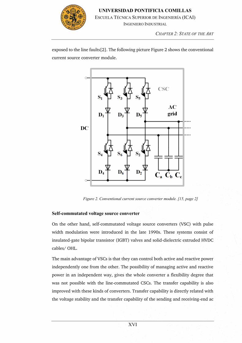
exposed to the line faults[2]. The following picture Figure 2 shows the conventional
current source converter module.
Self-commutated voltage source converter
On the other hand, self-commutated voltage source converters (VSC) with pulse
width modulation were introduced in the late 1990s. These systems consist of
insulated-gate bipolar transistor (IGBT) valves and solid-dielectric extruded HVDC
cables/ OHL.
The main advantage of VSCs is that they can control both active and reactive power
independently one from the other. The possibility of managing active and reactive
power in an independent way, gives the whole converter a flexibility degree that
was not possible with the line-commutated CSCs. The transfer capability is also
improved with these kinds of converters. Transfer capability is directly related with
the voltage stability and the transfer capability of the sending and receiving-end ac
Figure 2. Conventional current source converter module. [15, page 2]
CHAPTER 2: STATE OF THE ART
XVII
UNIVERSIDAD PONTIFICIA COMILLAS ESCUELA TÉCNICA SUPERIOR DE INGENIERÍA (ICAI)
INGENIERO INDUSTRIAL
systems. These two factors are improved due to the dynamic support that the
converter presents at each terminal.
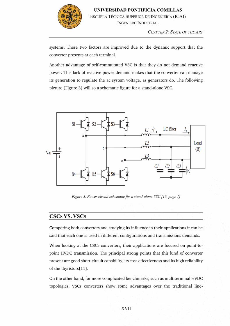
Another advantage of self-commutated VSC is that they do not demand reactive
power. This lack of reactive power demand makes that the converter can manage
its generation to regulate the ac system voltage, as generators do. The following
picture (Figure 3) will so a schematic figure for a stand-alone VSC.
CSCS VS. VSCS
Comparing both converters and studying its influence in their applications it can be
said that each one is used in different configurations and transmissions demands.
When looking at the CSCs converters, their applications are focused on point-to-
point HVDC transmission. The principal strong points that this kind of converter
present are good short-circuit capability, its cost-effectiveness and its high reliability
of the thyristors[11].
On the other hand, for more complicated benchmarks, such as multiterminal HVDC
topologies, VSCs converters show some advantages over the traditional line-
Figure 3. Power circuit schematic for a stand-alone VSC [16, page 1]

CHAPTER 2: STATE OF THE ART
XVIII
UNIVERSIDAD PONTIFICIA COMILLAS ESCUELA TÉCNICA SUPERIOR DE INGENIERÍA (ICAI)
INGENIERO INDUSTRIAL
commutated converters that make them much more efficient. The main benefits of
VSCs are [ETH]:
x The possibility to control active and reactive power independently
x Commutation trustworthiness
x Dynamic response
x Improvement in AC network short circuit capacity
x No reactive power demand
x Black-start capability
All these characteristics make voltage source converters a better option when
multiterminal networks are being treated. A multiterminal network is composed
with different branches. These branches have different performances regarding its
configurations and operation modes. The different possibilities that exist are:
x Asymmetric monopole
x Symmetric monopole
x Bipolar
x Combination
Asymmetric monopole
This kind of configuration is the simplest one, and as a result the less expensive one.
The requirements for these kinds of configurations are one converter per terminal
and one full insulated high voltage conductor. The disadvantage of this high voltage
conductor is that a constant DC current flows through ground. This current can
cause corrosion with all its implications, as damaging the transformers due to
saturation. Figure 4 shows an asymmetric monopole configuration.

CHAPTER 2: STATE OF THE ART
XIX
UNIVERSIDAD PONTIFICIA COMILLAS ESCUELA TÉCNICA SUPERIOR DE INGENIERÍA (ICAI)
INGENIERO INDUSTRIAL
Symmetric monopole
As differences from the asymmetric monopole configuration, no ground currents
flow during normal operation. Another important difference is the flexibility that it
offers. The two poles cannot operate in an independent way, but this configuration
allows to carry potential of opposite polarity. Figure 5 represents a symmetric
monopole configuration.
Figure 4. Asymmetric Monopole configuration. [11, page 16]
Figure 5. Symmetric Monopole configuration. [11, page 17]
CHAPTER 2: STATE OF THE ART
XX
UNIVERSIDAD PONTIFICIA COMILLAS ESCUELA TÉCNICA SUPERIOR DE INGENIERÍA (ICAI)
INGENIERO INDUSTRIAL
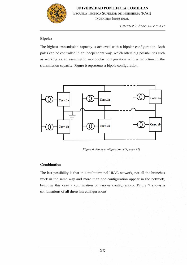
Bipolar
The highest transmission capacity is achieved with a bipolar configuration. Both
poles can be controlled in an independent way, which offers big possibilities such
as working as an asymmetric monopolar configuration with a reduction in the
transmission capacity. Figure 6 represents a bipole configuration.
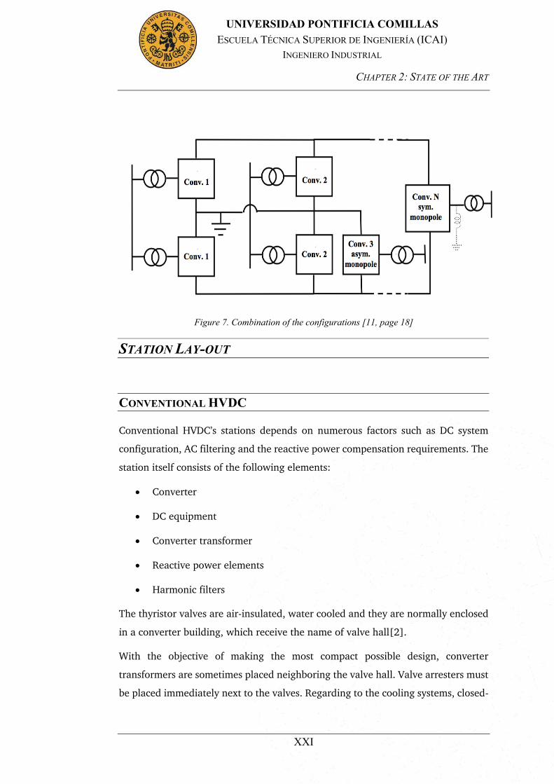
Combination
The last possibility is that in a multiterminal HDVC network, not all the branches
work in the same way and more than one configuration appear in the network,
being in this case a combination of various configurations. Figure 7 shows a
combinations of all three last configurations.
Figure 6. Bipole configuration. [11, page 17]
CHAPTER 2: STATE OF THE ART
XXI
UNIVERSIDAD PONTIFICIA COMILLAS ESCUELA TÉCNICA SUPERIOR DE INGENIERÍA (ICAI)
INGENIERO INDUSTRIAL
STATION LAY-OUT
CONVENTIONAL HVDC
Conventional HVDC’s stations depends on numerous factors such as DC system
configuration, AC filtering and the reactive power compensation requirements. The
station itself consists of the following elements:
x Converter
x DC equipment
x Converter transformer
x Reactive power elements
x Harmonic filters
The thyristor valves are air-insulated, water cooled and they are normally enclosed
in a converter building, which receive the name of valve hall[2].
With the objective of making the most compact possible design, converter
transformers are sometimes placed neighboring the valve hall. Valve arresters must
be placed immediately next to the valves. Regarding to the cooling systems, closed-
Figure 7. Combination of the configurations [11, page 18]

CHAPTER 2: STATE OF THE ART
XXII
UNIVERSIDAD PONTIFICIA COMILLAS ESCUELA TÉCNICA SUPERIOR DE INGENIERÍA (ICAI)
INGENIERO INDUSTRIAL
loop valves are used to circulate the cooling medium, which can be deionized water
or a mix of water and glycol, through the indoor thyristor valves. The AC system
voltage and the reactive power compensation requirements have big influence on
the area requirements. Each system requirements have its reactive power exchange
and its maximum voltage step. These requirements for each system makes that each
individual bank rating is limited by these conditions. In terms of the total space
used, the AC yard with filters and shunt compensation can cover up to three
quarters of the total area requirements. The following Figure 8, will show a
conventional HVDC station layout.
VSC-BASED HVDC
In these type of converters, the transmission circuit is formed by a bipolar two-wire
HVDC system. The presence of the DC capacitors is to provide a stiff DC voltage
source. AC phase reactors and power transformers are used for the coupling of the
converters to the AC system. Harmonic filters are located between the phase
reactors and power transformers, which is not common in most of the conventional
converters. This is done so that the transformers are not exposed to DC voltage
stresses or harmonic loading.
A set of series-connected IGBT positionsform the IGBT valves which are used in
VSC converters. Each complete IGBT position consists of:
x IGBT
x Antiparallel diode
x Gate unit
x Voltage divider
x Water-cooled heat sink
Figure 8. HVDC Conventional Station layout. From [2, page 41].
CHAPTER 2: STATE OF THE ART
XXIII
UNIVERSIDAD PONTIFICIA COMILLAS ESCUELA TÉCNICA SUPERIOR DE INGENIERÍA (ICAI)
INGENIERO INDUSTRIAL
Each gates unit includes gate-driving circuits, surveillance circuits and optical
interface. The gate driving electronics control the gate voltage, as well as the turn-
on and turn-off of the current. The goal of this control is to achieve optimal turn-on
and turn-off processes of the respective IGBT.
In case that the switching voltage needs to be higher than the rated voltage of one
IGBT, more positions are connected in series in order to achieve higher voltage
values. If this series connection is required, it is important to bear in mind that all
IBGTs must turn on and off at the same moment to achieve a uniformly distributed
voltage across the valve.
When the current is the limiting factor, and higher currents are required, the solution
comes from the paralleling of IGBT components or press packs.
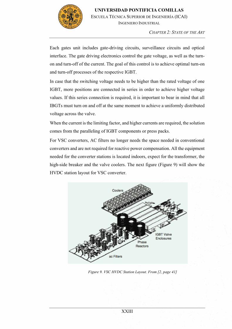
For VSC converters, AC filters no longer needs the space needed in conventional
converters and are not required for reactive power compensation. All the equipment
needed for the converter stations is located indoors, expect for the transformer, the
high-side breaker and the valve coolers. The next figure (Figure 9) will show the
HVDC station layout for VSC converter.
Figure 9. VSC HVDC Station Layout. From [2, page 41]

CHAPTER 2: STATE OF THE ART
XXIV
UNIVERSIDAD PONTIFICIA COMILLAS ESCUELA TÉCNICA SUPERIOR DE INGENIERÍA (ICAI)
INGENIERO INDUSTRIAL
TYPES OF FAULTS
In HVDC systems there are several types of failures on lines, which will lead to a
short circuit in the scheme. These type of faults are the following:
x Pole-to-ground faults
x Pole-to-pole faults
The thesis will put its focus on the pole-to-ground faults as they are considered to
be significantly more frequent than the pole-to-pole faults[11]. The main reasons
that lead to a pole-to-ground fault are the aging of the cable’s main insulation or
external damages. These situations provoke the breakdown of the cable insulation
and afterwards, that might lead to the pole-to-ground fault.
Once the breakdown has occurred in the cable insulation, an arc burns between the
pole and the sheath of the cable. Also, a ground loop through the sheath and the
next grounding point is established.
The current that flows through the arc experiments an increase in its value at high
speed. This increase in the current is the responsible for the destruction of the cable
at ground fault location. Once the cable is destructed, the arc now burns between
the pole and the ground. This arc is characterized by being a low-ohmic path for
the current.
On the other hand, after the ground fault occurs, the voltage behavior is different
to the current’s. In this case, the value of the voltage decreases to a level determined
by the fault resistance, the fault current and the characteristics of the soil. This drop
in the voltage is quick, but not instantaneously, which can be explained by the
voltage supporting of the distributed cable capacitance and the inductance in the
fault[11], [12] and [13].

CHAPTER 2: STATE OF THE ART
XXV
UNIVERSIDAD PONTIFICIA COMILLAS ESCUELA TÉCNICA SUPERIOR DE INGENIERÍA (ICAI)
INGENIERO INDUSTRIAL
MULTITERMINAL SYSTEMS
The majority of HVDC systems are used in point-to-point configurations. These
transmission systems are defined as two converter’s stations configurations, each
station located at each end of the line.
Historically, the idea of using HVDC systems not only for point-to-point
connections, but also for multiterminal networks has raised in several occasions. In
these networks, the power is exchanged at least between three power converters.
The first multiterminal networks that were connected via HVDC systems were
implanted in the 1980s and 1990s in Italy and Canada. These systems were based
on the previously discussed line-commutated converters. Due to the behavior of
these converters, the operation of the DC networks could not be done or only with
great effort.
The new generations of self-commutated power converters, makes the operation in
multiterminal networks possible due to its multiple advantages compared to the
line-commutated converters.
CURRENT EXISTING METHODS
At the moment two methods have been proposed with the objective of advancing
into a more standardized way to face the study of short-circuits in HVDC grids. In
both cases, the results obtained with the analytical equations proposed have been
compared with PSCAD simulations. PSCAD stands for Power System CAD and it is
a tool which allows to simulate the electrical behavior of a certain circuit. Besides
these two methods, a standard method exists for short circuit in DC grids.There
have also been other publications, which have helped the following publications
such as: [3],[4],[5],[6],[7],[8],[9] and [10]. Some of these public publications
were written by the authors of the methods which are going to be compared. This
previous work helped them to get a better understanding of the transient process
of the current when a short circuit occurs. These previous publications are related
to the understanding of short circuit current transient. Also, different types of
converters are studied (six pulse bridge, two-level converters).
CHAPTER 2: STATE OF THE ART
XXVI
UNIVERSIDAD PONTIFICIA COMILLAS ESCUELA TÉCNICA SUPERIOR DE INGENIERÍA (ICAI)
INGENIERO INDUSTRIAL
STANDARD IEC 61660
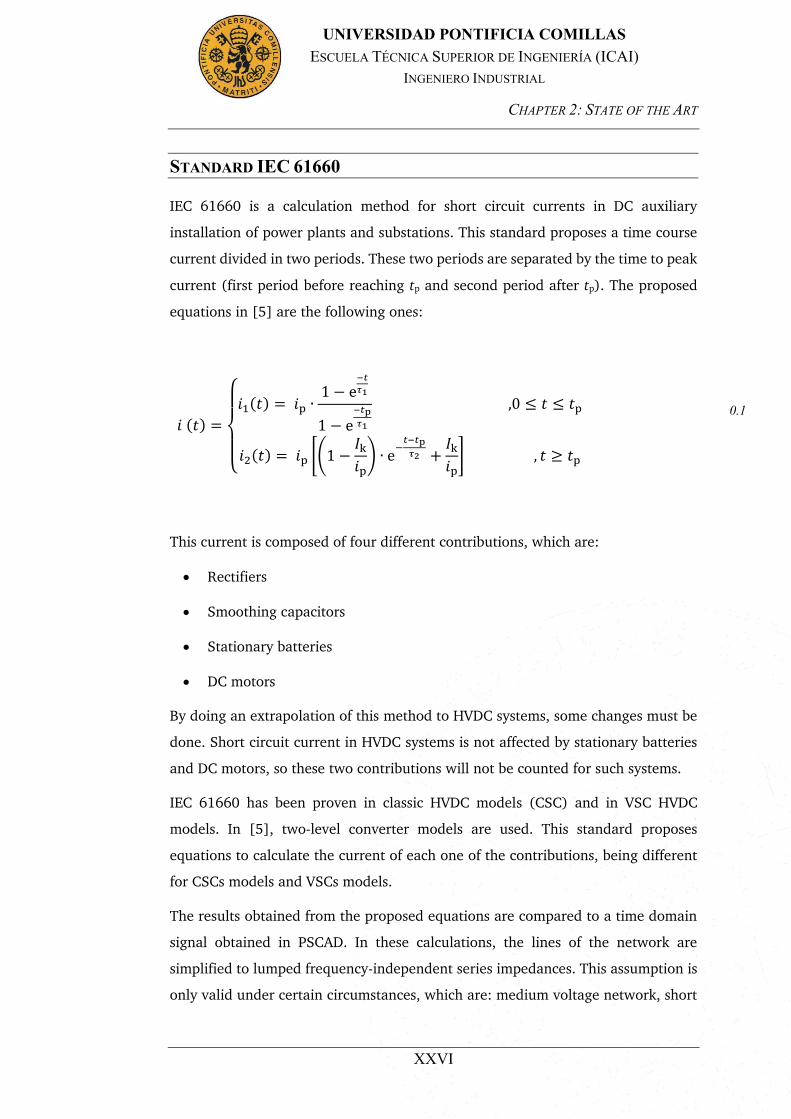
IEC 61660 is a calculation method for short circuit currents in DC auxiliary
installation of power plants and substations. This standard proposes a time course
current divided in two periods. These two periods are separated by the time to peak
current (first period before reaching tp and second period after tp). The proposed
equations in [5] are the following ones:
𝑖 (𝑡) =
𝑖1(𝑡) = 𝑖p ∙
1 − e−𝑡𝜏1
1 − e−𝑡p𝜏1
,0 ≤ 𝑡 ≤ 𝑡p
𝑖2(𝑡) = 𝑖p [(1 −𝐼k𝑖p) ∙ e−
𝑡−𝑡p𝜏2 +
𝐼k𝑖p] , 𝑡 ≥ 𝑡p
0.1
This current is composed of four different contributions, which are:
x Rectifiers
x Smoothing capacitors
x Stationary batteries
x DC motors
By doing an extrapolation of this method to HVDC systems, some changes must be
done. Short circuit current in HVDC systems is not affected by stationary batteries
and DC motors, so these two contributions will not be counted for such systems.
IEC 61660 has been proven in classic HVDC models (CSC) and in VSC HVDC
models. In [5], two-level converter models are used. This standard proposes
equations to calculate the current of each one of the contributions, being different
for CSCs models and VSCs models.
The results obtained from the proposed equations are compared to a time domain
signal obtained in PSCAD. In these calculations, the lines of the network are
simplified to lumped frequency-independent series impedances. This assumption is
only valid under certain circumstances, which are: medium voltage network, short
CHAPTER 2: STATE OF THE ART
XXVII
UNIVERSIDAD PONTIFICIA COMILLAS ESCUELA TÉCNICA SUPERIOR DE INGENIERÍA (ICAI)
INGENIERO INDUSTRIAL
interconnections and small line capacitances. In HVDC systems, these circumstances
are not real, and for instance, the capacitance cannot be neglected [11] and [5].
Taking all these into consideration, this comes to achieve reliable results only con
certain circumstances, which are the following ones: lines are relatively short, and
the DC capacitor and pole reactor are high[11]. Under these circumstances, the
lumped element become dominant over the frequency-dependent distributed line
parameters. As the goal of a standard for HVDC systems is the good performance of
the model in every situation, the IEC 61660 is dismissed for the purpose.
PHD OF ETH ZURICH
This PhD [11]studies transient fault currents in HVDC VSC Network during pole-
to-ground faults. It proposes analytic approximation of fault currents from the
different contributions of the system.
The network model, which is going to be used, consists of a converter, a DC
capacitor and a busbar, which gathers the different lines that converge at that point.
Figure 10 shows the network. All these elements in the system have an influence
on the short-circuit current and are considered in different equations.
The author divides the short-circuit current into different contributions. One of the
contributions are the capacitive sources and the other one the AC Network
contribution.
It is important to notice the influence that both contributions have on the total
current. The short circuit current during the first few ms after the fault has occurred
is dominated by the capacitive sources. In this period, the AC side can be neglected,
due to its weak influence[11].
Once this period is over, the next period's behavior is the opposite that the one seen
before. The period begins with little influence of the capacitive sources, being the
steady-state short circuit exclusively fed by the AC network contribution.
Further variations on different parameters of the system such as fault resistance,
DC capacitors, network topology or impedances are done in order to see the
parameter's influence.
CHAPTER 2: STATE OF THE ART
XXVIII
UNIVERSIDAD PONTIFICIA COMILLAS ESCUELA TÉCNICA SUPERIOR DE INGENIERÍA (ICAI)
INGENIERO INDUSTRIAL
Capacitive Sources
For the capacitive sources contribution, the equations proposed are obtained based
on the planar skin effect and the individual surges. These equations are proven on
cable networks, but they can also be applied to OHL configurations.
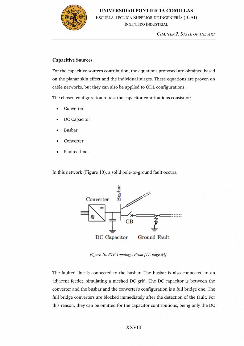
The chosen configuration to test the capacitor contributions consist of:
x Converter
x DC Capacitor
x Busbar
x Converter
x Faulted line
In this network (Figure 10), a solid pole-to-ground fault occurs.
The faulted line is connected to the busbar. The busbar is also connected to an
adjacent feeder, simulating a meshed DC grid. The DC capacitor is between the
converter and the busbar and the converter's configuration is a full bridge one. The
full bridge converters are blocked immediately after the detection of the fault. For
this reason, they can be omitted for the capacitor contributions, being only the DC
Figure 10. PTP Topology. From [11, page 84]

CHAPTER 2: STATE OF THE ART
XXIX
UNIVERSIDAD PONTIFICIA COMILLAS ESCUELA TÉCNICA SUPERIOR DE INGENIERÍA (ICAI)
INGENIERO INDUSTRIAL
capacitor and the adjacent feeder the elements that contribute to the short circuit
current.
The capacitive sources contributions also include a division and studies all the
elements that belong to them. In the studied system, the DC capacitor and the
adjacent feeder are the components which are going to be studied.
The short circuit current that the DC capacitor adds to the system is derived from
the voltage that the capacitor experiments. This voltage can be defined as the sum
of the forward and reflected, backward travelling wave. The voltage value, the
length at which the fault occurs, the reflection coefficient and the travelling wave
determine the voltage in the DC capacitor in the Laplace domain.
As the voltage and the current fulfill this equation in the time domain, the voltage
should be transformed into this domain. This transformation can be done in two
different ways: the first one is an exact transformation and the second one is an
approximation. For the thesis purposes, the approximation method satisfies our
requirements and the formulas obtained are used.
The adjacent feeder contribution is referred to the transmission through the busbar
into the neighboring feeder of the incident negative voltage surge. This surge is
initiated at the ground fault location. The neighboring feeder is, thus, discharged,
contributing in this way to the total fault current in the CB.
Unlike the DC Capacitor short circuit current, the adjacent feeder short circuit
current is calculated with the help of the travelling wave directly in the Laplace
domain. With the supposition of the adjacent feeder being infinitely long, there is
no backward travelling wave to be considered. This current must also be
transformed, in order to be able to work with both contributions in the same domain.
Again, two different alternatives are presented: exact transformation and
approximation. For the same reasons explained before, the approximation formulas
are accurate enough to use them. These equations were proposed in [11], [12] and
[13].

CHAPTER 2: STATE OF THE ART
XXX
UNIVERSIDAD PONTIFICIA COMILLAS ESCUELA TÉCNICA SUPERIOR DE INGENIERÍA (ICAI)
INGENIERO INDUSTRIAL
𝑣c(𝑡) = 𝑉0 ∙ 𝑒𝑟𝑓𝑐(𝛼 𝜏
2 √𝑡 − 𝜏) ∙ (e−
2𝐶𝑅0
(𝑡−𝜏) − 1) ∙ 𝜎(𝑡 − 𝜏) (0.2)
𝑖c(𝑡) = −𝐶𝑑𝑣c𝑑𝑡= −𝑉0
∙ [exp(−𝛼2𝜏2
4(𝑡 − 𝜏)) ∙ (𝑡 − 𝜏)−3 2⁄ ∙ (e
−2𝐶𝑅0
(𝑡−𝜏) − 1)
−2𝐶𝑅0
∙ e−2𝐶𝑅0
(𝑡−𝜏) ∙ 𝑒𝑟𝑓𝑐 (𝛼𝜏
2√𝑡 − 𝜏)] ∙ 𝜎(𝑡 − 𝜏)
(0.3)
Once both contributions have been transformed into the time domain, the sum of
both of them represent the short circuit current that flows through the circuit
breaker when a fault line to ground occurs.
The implementation of these formulas into Matlab leads to time domain signals,
which represent the behavior of the current and voltage in the transient period of
the short-circuit.
AC Network contribution
This second contribution is responsible of the AC Network infeed. It is noteworthy
that not both contributions have their highest impact at the same time. On the one
hand, the just discussed capacitor sources have their highest impact during the first
few ms of the transient period. Once this period is over, the AC network contribution
takes over and becomes the one that defines the total short circuit current. In fact,
it can be defined as a gradual process, where the AC infeed starts with almost none
importance, at the time when the fault occurs, and gains importance over the
capacitive sources the following ms. In the steady state, the short circuit current is
only fed by the AC Network contribution.
CHAPTER 2: STATE OF THE ART
XXXI
UNIVERSIDAD PONTIFICIA COMILLAS ESCUELA TÉCNICA SUPERIOR DE INGENIERÍA (ICAI)
INGENIERO INDUSTRIAL
The publication proposes new analytical expressions, also for this second period in
point-to-point connections and multiterminal DC systems. The author reached the
conclusion that the, until the time, existing equations that defined the transient
process were not accurate enough and only applicable to certain situations.
The presented equations are valid regardless the line configurations (both cable and
OHL achieve good results) and the type of fault (pole-to-ground or pole-to-pole).
Nevertheless, in his publications, only cable pole-to-ground faults results are
presented.
The study makes a difference for the different configurations that the grid can have.
The network can consist only of two nodes, which is represented as a point-to-point
configuration or it can have more nodes, being in this case a multiterminal network.
As it was already said, equations for both situations are provided.
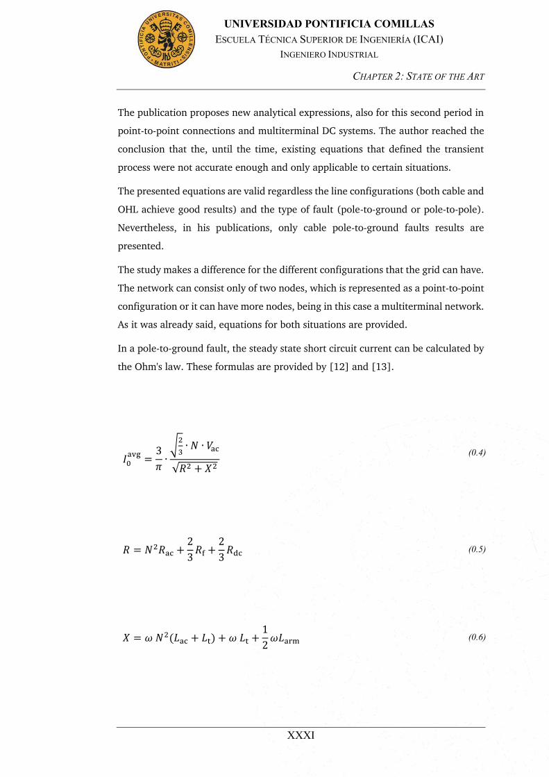
In a pole-to-ground fault, the steady state short circuit current can be calculated by
the Ohm's law. These formulas are provided by [12] and [13].
𝐼0avg =
3𝜋∙√23∙ 𝑁 ∙ 𝑉ac
√𝑅2 + 𝑋2 (0.4)
𝑅 = 𝑁2𝑅ac +23𝑅f +
23𝑅dc (0.5)
𝑋 = 𝜔 𝑁2(𝐿ac + 𝐿t) + 𝜔 𝐿t +12𝜔𝐿arm (0.6)

CHAPTER 2: STATE OF THE ART
XXXII
UNIVERSIDAD PONTIFICIA COMILLAS ESCUELA TÉCNICA SUPERIOR DE INGENIERÍA (ICAI)
INGENIERO INDUSTRIAL
To do so, the voltage will be divided by the impedance in the steady state and the
result will be the resulting current. The phase-to-phase voltage is Vac, the reactances
that have an impact on this state of the transient are the transformer reactance Lt,
the phase reactor LS and the armature reactance. The inductances in the DC side
can be omitted for the calculation of this current. AC and transformer reactances
will need to be multiplied by the transformer turns ratio to the power of two. The
resistances used in the formula are the resistance of the faulted cable RDC, and the
fault resistance. As well as AC inductance, the AC resistance will also be multiplied
by the transformer turns ratio to the power of two.
As it was exposed before, the systems which are going to be studied will be point-
to-point and multiterminal configurations. The formulas for the multiterminal
networks were not provided by[12], but the Phd [11] derives the formulas for these
situations.
STEADY STATE CURRENT
- The point-to-point configurations can be derived in a similar way than (0.4). With
the help of Kirchhoff's Current Law (KCL), the following equations are proposed. In
a situation, where the fault resistance is zero, equations (0.4) and (0.7) are
equivalent.
𝐼0avg =
3𝜋∙ √2
3∙ 𝑁1 ∙ 𝑉ac1 (𝑍2 +
23𝑅f) −
3𝜋∙ √2
3∙ 𝑁2 ∙ 𝑉ac2 ∙
23𝑅f
𝑍1𝑍2 +23𝑅f𝑍1 +
23𝑅f𝑍2
(0.7)
CHAPTER 2: STATE OF THE ART
XXXIII
UNIVERSIDAD PONTIFICIA COMILLAS ESCUELA TÉCNICA SUPERIOR DE INGENIERÍA (ICAI)
INGENIERO INDUSTRIAL
𝑍𝑖 = 𝑗𝜔 (𝐿ac,𝑖𝑁𝑖2 + 𝐿t,𝑖𝑁𝑖2 + 𝐿s,𝑖 +12𝐿arm,𝑖) + 𝑅ac,𝑖𝑁𝑖2
+23𝑅dc,𝑖 , 𝑖 = 1,2
(0.8)
- On the other hand, when handling with multiterminal topologies, the approach to
reach the steady state short circuit current is not exactly the same. For the treatment
of it, it is expressed a system of linear equations. The topology is divided by the
number of terminals present in the configuration. For a l-terminal system, l +1
linear equations will be studied. The additional linear equation, comes from the
ground fault.
[𝑌dc +23𝑌ac] ∙
[ 𝑣dc,1𝑣dc,2…𝑣dc,𝑛𝑣f ]
= 3𝜋∙ 𝑌ac ∙
[ 𝑣0,1𝑣0,2…𝑣0,𝑛0 ] (0.9)
The elements of these matrixes can be calculated following the next
equations(0.10)-(0.12).
𝑌dc,𝑖𝑗 =
𝑦dc,𝑖𝑖 +∑𝑦dc,𝑖𝑗𝑖≠𝑗
if 𝑖 = 𝑗
−𝑦dc,𝑖𝑗if 𝑖 ≠ 𝑗
(0.10)
CHAPTER 2: STATE OF THE ART
XXXIV
UNIVERSIDAD PONTIFICIA COMILLAS ESCUELA TÉCNICA SUPERIOR DE INGENIERÍA (ICAI)
INGENIERO INDUSTRIAL
𝑌ac,𝑖𝑖 = [𝑁𝑖2(𝑗𝜔𝐿ac,𝑖 + 𝑗𝜔𝐿t,𝑖 + 𝑅ac,𝑖) + 𝑗𝜔 (𝐿s,𝑖 +12𝐿arm,𝑖)]−1 (0.11)
𝑣0𝑖 = √23𝑁𝑖 ∙ 𝑉ac,𝑖 (0.12)
Ydc matrix represents the admittance matrix of the DC part of the topology, which
includes the faulted node and has (n+1)x(n+1) dimensions. Yac matrix represents
the admittance matrix of AC part of the network. In this case, the faulted node is
also included, having, thus, the same dimensions as the previous matrix. As Yac
represents the AC side of the topology, the elements of it corresponding the fault
node will be zero.
TRANSIENT CURRENT
For the transient current it is important to consider as a start point that the exact
time development from all the transient contributions cannot be exactly represented
analytically and the formulas that are proposed in [11] are derived from the peak
value.
The two contributions studied in this PhD have the peak values at different points
and the dimensioning criteria which is used for the derivation of the following
equation is that the peak current for the capacitor contributions occur at 2 ms and
the peak current for the AC infeed at 13 ms. Assuming this and with the help of the
solution of an underdamped, oscillating second order system, the following time
domain current equation is proposed:

CHAPTER 2: STATE OF THE ART
XXXV
UNIVERSIDAD PONTIFICIA COMILLAS ESCUELA TÉCNICA SUPERIOR DE INGENIERÍA (ICAI)
INGENIERO INDUSTRIAL
𝑖cb(𝑡) =𝜋3∙ 𝐼0avg 1 − e−𝜍𝑀𝑇𝜔T1(𝑡−𝑇)
∙ [cos(𝜔MT(𝑡 − 𝑇)) +𝜍MT
√1 − 𝜍MT2
∙ sin(𝜔MT(𝑡 − 𝑇))] ∙ 𝑢(𝑡 − 𝑇)
(0.13)
𝑇 = 𝑙𝑐 (0.14)
𝑐 = 1√𝐿𝐶
(0.15)
For the calculation of the damping factor, the method exposed in [11] will be used
and the equations required are the following ones (0.16)-(0.25)
𝜍MT = 𝜍T1 ∙𝛼T1 + 𝛼MT
𝛼T1 (0.16)
𝛼T1 =𝑅𝜔𝑋
(0.17)
𝛼MT = 𝑅eq𝐿eq
(0.18)
CHAPTER 2: STATE OF THE ART
XXXVI
UNIVERSIDAD PONTIFICIA COMILLAS ESCUELA TÉCNICA SUPERIOR DE INGENIERÍA (ICAI)
INGENIERO INDUSTRIAL
𝜍MT = 𝜍T1 ∙𝛼T1 + 𝛼MT
𝛼T1 (0.19)
𝑅eq = [1𝑅1f
+1
𝑅13 + (1𝑅23
+ 1𝑅34
+ 1𝑅24)−1+ 𝑅2f
]
−1
+ 𝑅f (0.20)
𝐿eq = [1𝐿1f
+1
𝐿13 + (1𝐿23+ 1𝐿34+ 1𝐿24)−1+ 𝐿2f
]
−1
(0.21)
𝜍T1 = √1 −
𝜋2
𝜋2 + (ln (𝐼maxT1 −𝐼0
T1,avg
𝐼0T1,avg ))
2 (0.22)
𝜔T1 = 𝜋
2𝜙T1𝜔
∙ √1 − 𝜍T12 (0.23)
𝜙T1 = arctan (𝑋𝑅)
(0.24)
𝜔MT = 𝜔T1√1 − 𝜍MT2 (0.25)
CHAPTER 2: STATE OF THE ART
XXXVII
UNIVERSIDAD PONTIFICIA COMILLAS ESCUELA TÉCNICA SUPERIOR DE INGENIERÍA (ICAI)
INGENIERO INDUSTRIAL
TU DARMSTADT DISSERTATION
In this dissertation[14], the author proposes equations for different parameters of
the short-circuit transient current response after the fault. These parameters are
time to peak, steady state short-circuit current, short-circuit current initial slope and
current peak.
Unlike the PhD from Zurich, this dissertation studies four different converters:
x Six-pulse bridge
x Twelve-pulse bridge
x Two-point converter
x Modular multi-level converter
All of these converters are studied for monopolar and bipolar configurations, so
equations for eight different configurations are provided.
Another difference that can be easily found between the two studies is that the TU
Darmstadt's formulas give special point of the time course, while the PhD from
Zurich gives time domain signals as results. In the future comparison, these
characteristic points from the current (steady state and peak current) will be
obtained from the time course result of the PhD and compared to the values from
the TU Darmstadt method.
The goal of the thesis is to compare both methods and see which one yields better
results for different situations. To achieve that goal, only the configurations that
can be compared in both methods will be implemented. In this case, only two-level
converter configuration will be studied.
The two-point converter is one of the self-commutated converters with switch-off
IGBTs that are connected in anti-parallel to diodes. In the event of a short-circuit
CHAPTER 2: STATE OF THE ART
XXXVIII
UNIVERSIDAD PONTIFICIA COMILLAS ESCUELA TÉCNICA SUPERIOR DE INGENIERÍA (ICAI)
INGENIERO INDUSTRIAL
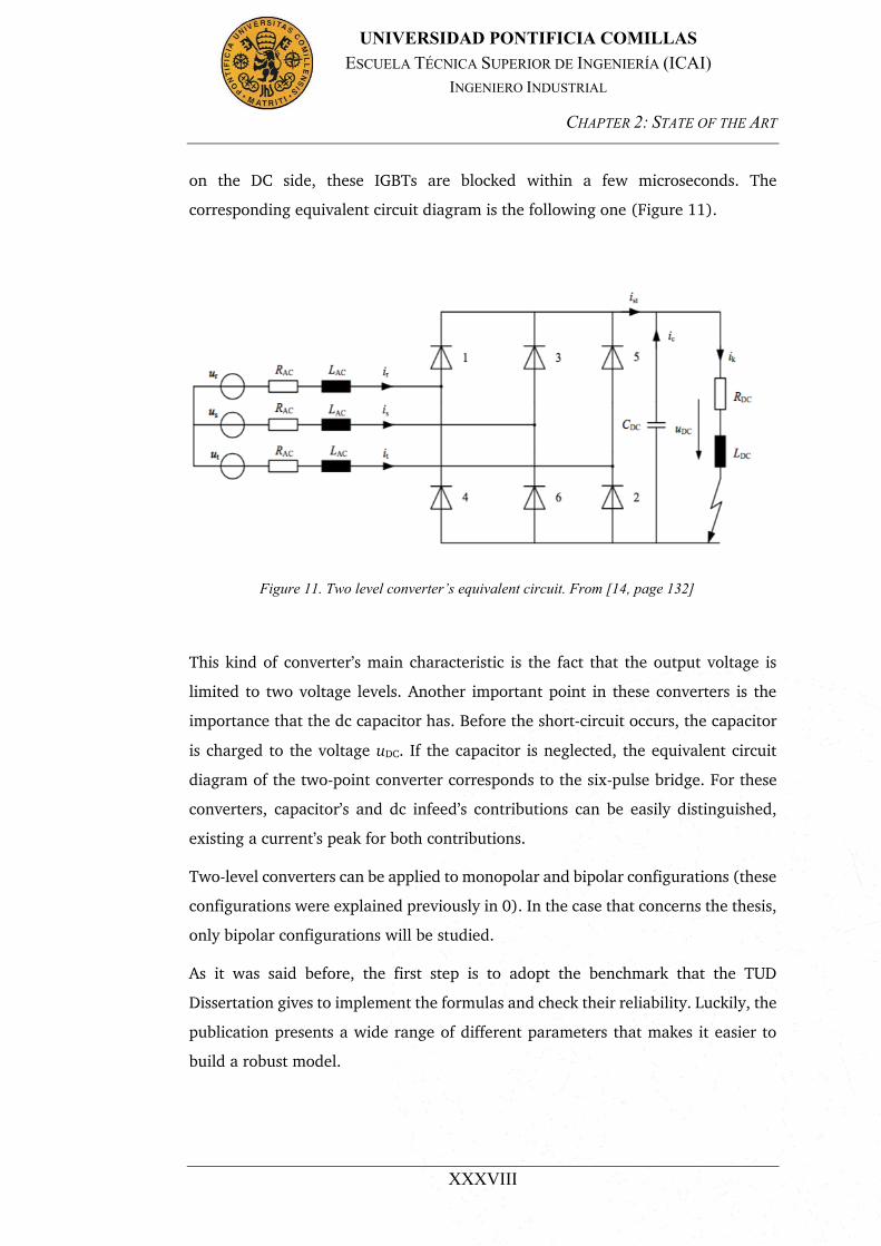
on the DC side, these IGBTs are blocked within a few microseconds. The
corresponding equivalent circuit diagram is the following one (Figure 11).
This kind of converter’s main characteristic is the fact that the output voltage is
limited to two voltage levels. Another important point in these converters is the
importance that the dc capacitor has. Before the short-circuit occurs, the capacitor
is charged to the voltage uDC. If the capacitor is neglected, the equivalent circuit
diagram of the two-point converter corresponds to the six-pulse bridge. For these
converters, capacitor’s and dc infeed’s contributions can be easily distinguished,
existing a current’s peak for both contributions.
Two-level converters can be applied to monopolar and bipolar configurations (these
configurations were explained previously in 0). In the case that concerns the thesis,
only bipolar configurations will be studied.
As it was said before, the first step is to adopt the benchmark that the TUD
Dissertation gives to implement the formulas and check their reliability. Luckily, the
publication presents a wide range of different parameters that makes it easier to
build a robust model.
Figure 11. Two level converter’s equivalent circuit. From [14, page 132]
CHAPTER 2: STATE OF THE ART
XXXIX
UNIVERSIDAD PONTIFICIA COMILLAS ESCUELA TÉCNICA SUPERIOR DE INGENIERÍA (ICAI)
INGENIERO INDUSTRIAL
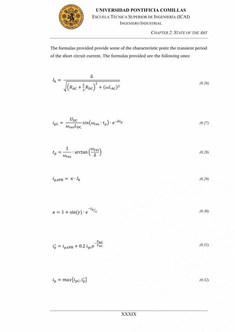
The formulas provided provide some of the characteristic point the transient period
of the short circuit current. The formulas provided are the following ones:
𝐼k =
√(𝑅AC +23𝑅DC)
2+ (𝜔𝐿AC)2
(0.26)
𝑖pC = 𝑈DC
𝜔res𝐿DC𝑠𝑖𝑛(𝜔res ∙ 𝑡p) ∙ e−𝛿𝑡p (0.27)
𝑡p =1𝜔res
∙ arctan (𝜔res𝛿) (0.28)
𝑖p,6PB = 𝜅 ∙ 𝐼k (0.29)
𝜅 = 1 + sin (𝛾) ∙ e−𝑡p
𝜏⁄ (0.30)
𝑖p∗ = 𝑖p,6PB + 0.2 𝑖pce−𝑅AC𝑋AC (0.31)
𝑖p = 𝑚𝑎𝑥𝑖pC, 𝑖p∗ (0.32)

CHAPTER 2: STATE OF THE ART
XL
UNIVERSIDAD PONTIFICIA COMILLAS ESCUELA TÉCNICA SUPERIOR DE INGENIERÍA (ICAI)
INGENIERO INDUSTRIAL
𝛿 = 𝑅DC2𝐿DC
(0.33)
𝜔02 = 1
𝐿DC𝐶DC (0.34)
CHAPTER 3: IMPLEMENTATION
XLI
UNIVERSIDAD PONTIFICIA COMILLAS ESCUELA TÉCNICA SUPERIOR DE INGENIERÍA (ICAI)
INGENIERO INDUSTRIAL
CHAPTER 3 : IMPLEMENTATION
PHD METHOD
The implementation of the formulas proposed in the ETH PhD, was done in Matlab,
with ".m" files. The thesis proposes formulas for the different contributions of the
electrical system. The procedure followed here was the following:
x Independent implementation for the different contributions
x Checking the reliability of the formulas with PSCAD simulations
x Superposition of the contributions
x Comparison with PSCAD simulations
INDEPENDENT IMPLEMENTATION FOR THE DIFFERENT CONTRIBUTIONS
This is the first part of the process. Here, the proposed formulas in the PhD are
studied and implemented in Matlab. The different contributions that the author
proposes are: Capacitive sources contributions and AC Network contribution.
Capacitive sources contributions are subdivided into DC capacitor's current and the
adjacent feeder's current contribution, while AC network contribution is just one
equation.
At this point, the benchmark and the system parameters were the same proposed
in the original publication. By selecting the same parameters, the graphics obtained
could be compared to the ones in the PhD.
The formulas given in the thesis [11], were not the correct ones, as the results were
not the expected ones, and the calculations of the right formula was done.
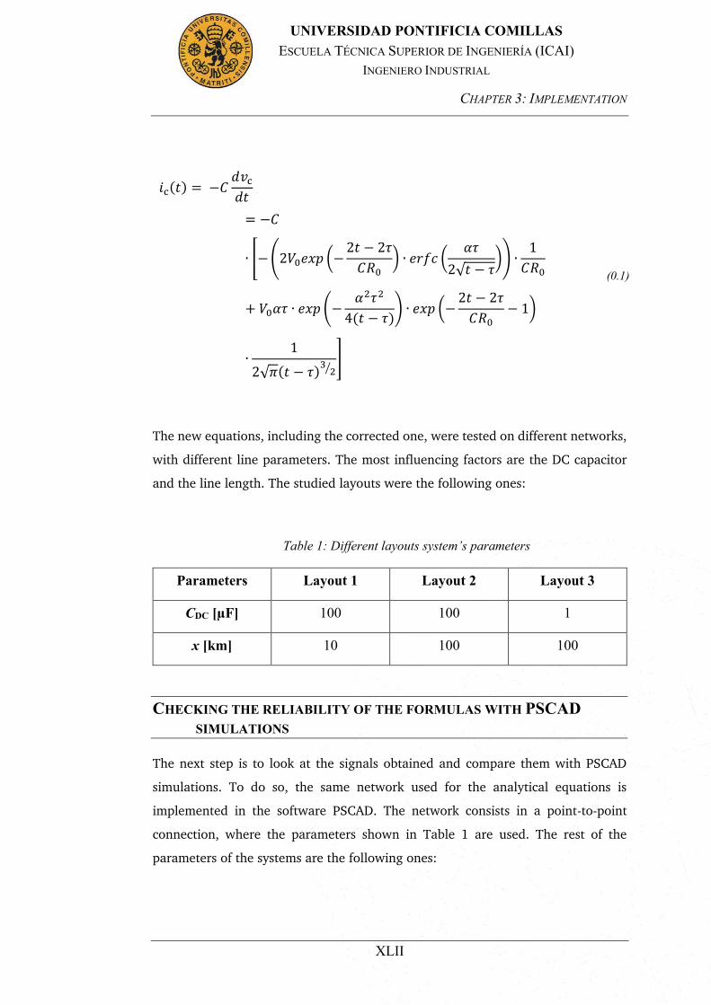
The new equation provided results much more accurate and similar to the provided
ones. This equation is the following:
CHAPTER 3: IMPLEMENTATION
XLII
UNIVERSIDAD PONTIFICIA COMILLAS ESCUELA TÉCNICA SUPERIOR DE INGENIERÍA (ICAI)
INGENIERO INDUSTRIAL
𝑖c(𝑡) = −𝐶𝑑𝑣c𝑑𝑡= −𝐶
∙ [−(2𝑉0𝑒𝑥𝑝 (−2𝑡 − 2𝜏𝐶𝑅0
) ∙ 𝑒𝑟𝑓𝑐 (𝛼𝜏
2√𝑡 − 𝜏)) ∙
1𝐶𝑅0
+ 𝑉0𝛼𝜏 ∙ 𝑒𝑥𝑝 (−𝛼2𝜏2
4(𝑡 − 𝜏)) ∙ 𝑒𝑥𝑝 (−
2𝑡 − 2𝜏𝐶𝑅0
− 1)
∙1
2√𝜋(𝑡 − 𝜏)32⁄]
(0.1)
The new equations, including the corrected one, were tested on different networks,
with different line parameters. The most influencing factors are the DC capacitor
and the line length. The studied layouts were the following ones:
Table 1: Different layouts system’s parameters
Parameters Layout 1 Layout 2 Layout 3
CDC [µF] 100 100 1
x [km] 10 100 100
CHECKING THE RELIABILITY OF THE FORMULAS WITH PSCAD SIMULATIONS
The next step is to look at the signals obtained and compare them with PSCAD
simulations. To do so, the same network used for the analytical equations is
implemented in the software PSCAD. The network consists in a point-to-point
connection, where the parameters shown in Table 1 are used. The rest of the
parameters of the systems are the following ones:

CHAPTER 3: IMPLEMENTATION
XLIII
UNIVERSIDAD PONTIFICIA COMILLAS ESCUELA TÉCNICA SUPERIOR DE INGENIERÍA (ICAI)
INGENIERO INDUSTRIAL
Table 2. System’s parameters
Parameters
Rated converter power 450 MW
DC Voltage 320 kV
AC Voltage 400 kV
SCR of AC Network 20
X/R of AC Networks 10
Transformer leakage
reactance 0.1 p.u
Transformer Turns Ratio 270/400
Converter Phase Reactor 0.05 p.u
CDC 10 – 100 µF
Rf 0 – 4 Ω
Line length 10 – 100 km
These different systems lead to the following current waveforms in the time domain.
In the original publication [11], the author describes a correction factor that is
applied to the different contributions. This correction factor is visually estimated
and set to 0.88. In the simulations done, three different factors were tested in order
to compare which one lead to a better performance. The three different factors were
0.75, 0.88 and 1. In the following pictures the results are shown with the best
correction factors, which were 0.88 and 1. It has been proved that the best result
was when the factor of 0.88 was used, as the author described in the original thesis.
Due to this, the figures will show the behavior of the current when this factor is
applied (Figure 12-Figure 14). The selected layout is the third one, where the values
CHAPTER 3: IMPLEMENTATION
XLIV
UNIVERSIDAD PONTIFICIA COMILLAS ESCUELA TÉCNICA SUPERIOR DE INGENIERÍA (ICAI)
INGENIERO INDUSTRIAL
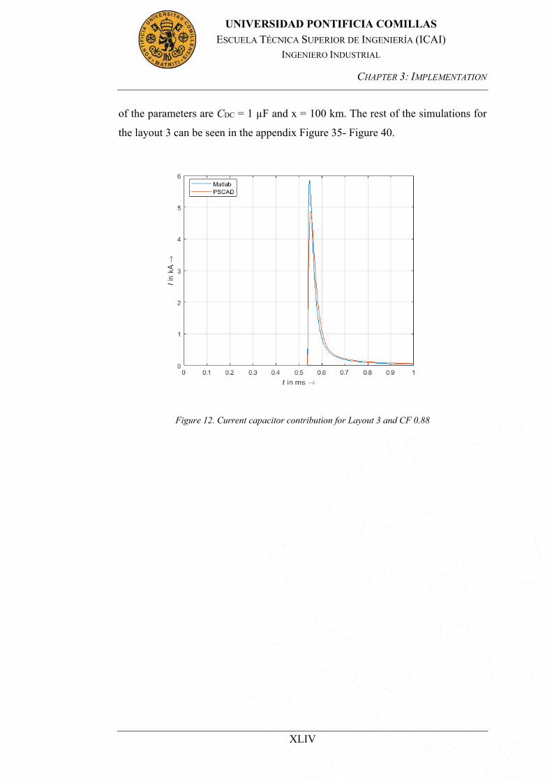
of the parameters are CDC = 1 µF and x = 100 km. The rest of the simulations for
the layout 3 can be seen in the appendix Figure 35- Figure 40.
Figure 12. Current capacitor contribution for Layout 3 and CF 0.88

CHAPTER 3: IMPLEMENTATION
XLV
UNIVERSIDAD PONTIFICIA COMILLAS ESCUELA TÉCNICA SUPERIOR DE INGENIERÍA (ICAI)
INGENIERO INDUSTRIAL
Figure 13.Current adjacent feeder contribution for Layout 3 and CF 0.88
Figure 14. CB Current for Layout 3 and CF 0.88

CHAPTER 3: IMPLEMENTATION
XLVI
UNIVERSIDAD PONTIFICIA COMILLAS ESCUELA TÉCNICA SUPERIOR DE INGENIERÍA (ICAI)
INGENIERO INDUSTRIAL
In this layout, the objective is to check how the systems behaves when the value of
the DC capacitor is very low (1 µF) and the distance to fault is 100 km. Observing
the three previous figures, it is seen that the current capacitor contribution is almost
1 kA higher in the peak moment, while in the rest of the time course both waves
match accurately.
On the other hand, the Matlab simulation is slightly lower for the adjacent feeder
contribution in the peak value. Overall, when both contributions are superposed,
the CB current present a very good behavior and the time domain signal can be said
to be reliable.
The figures of the first and the second layout are attached in the appendix of the
thesis. The observed behavior of those two layouts will be described in the
following paragraphs.
In the first layout, the distance to the fault location is 10 km and the DC capacitor
has a value of 100µF. With these conditions and a correction factor of 0.88the
obtained results are shown for the first ms. In the simulation it was be observed
how the number of surges seen in the PSCAD simulations are 9 for the specified
time, while the Matlab analytic simulation only represent one. The original PhD
proposes a formula for the subsequent surges, but it is only valid for the first two-
three surges, and afterwards does not give reliable results. This situation is also
attached in the appendix Figure 41.
Furthermore, the PSCAD model stablished to obtain these results (in this layout) is
not a realistic one and the future topologies and parameters will not lead to these
results (more than one surge and currents of 60 kA).
On the other hand, the second layout yield to more realistic results than the first
one. In this case, the distance to the fault is 100 km and the dc capacitor value is
100µF. These contributions can be seen to be important only in the first few ms.
That is the reason that the simulated time for these simulations is only 1 ms. In this
layout, with the set of parameters chosen, the current capacitor contribution
experiments an error of about 2 kA, while the current adjacent feeder contribution
follows better the expected value of current.
CHAPTER 3: IMPLEMENTATION
XLVII
UNIVERSIDAD PONTIFICIA COMILLAS ESCUELA TÉCNICA SUPERIOR DE INGENIERÍA (ICAI)
INGENIERO INDUSTRIAL
Analyzing the simulations and comparing them to the original and PSCAD
simulation ones it can be said that the implementation of the capacitive sources
currents is done correctly.
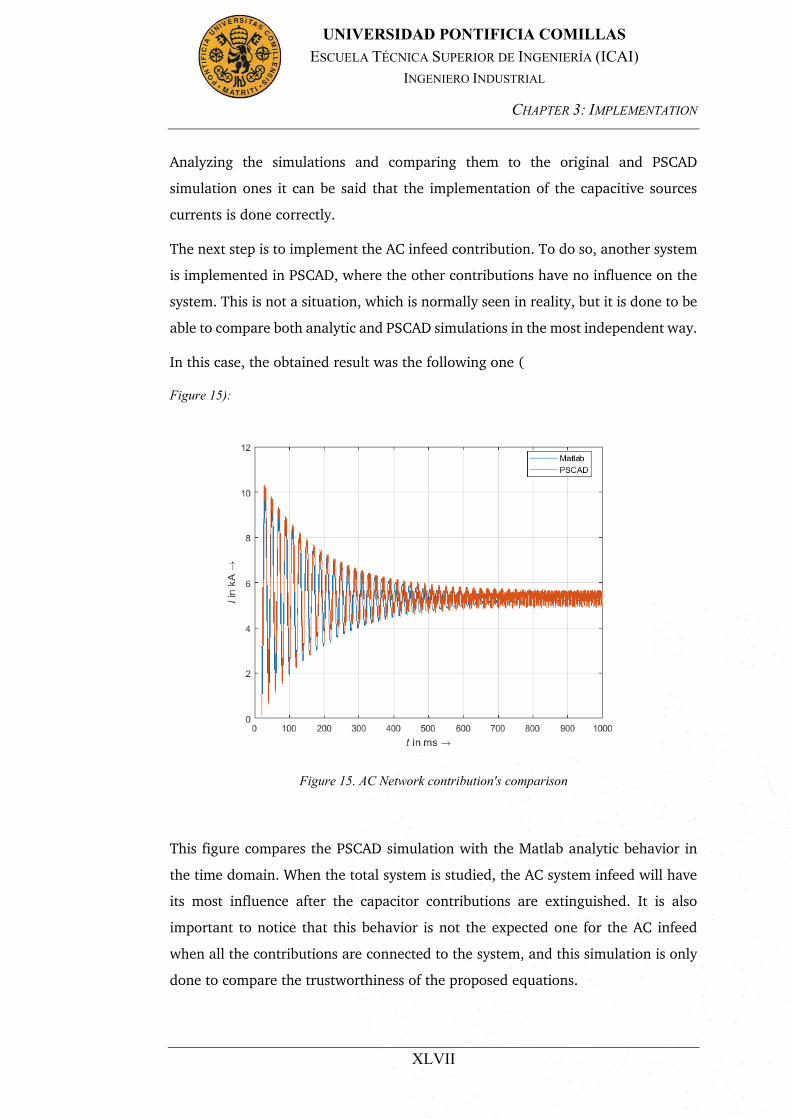
The next step is to implement the AC infeed contribution. To do so, another system
is implemented in PSCAD, where the other contributions have no influence on the
system. This is not a situation, which is normally seen in reality, but it is done to be
able to compare both analytic and PSCAD simulations in the most independent way.
In this case, the obtained result was the following one (
Figure 15):
Figure 15. AC Network contribution's comparison
This figure compares the PSCAD simulation with the Matlab analytic behavior in
the time domain. When the total system is studied, the AC system infeed will have
its most influence after the capacitor contributions are extinguished. It is also
important to notice that this behavior is not the expected one for the AC infeed
when all the contributions are connected to the system, and this simulation is only
done to compare the trustworthiness of the proposed equations.
CHAPTER 3: IMPLEMENTATION
XLVIII
UNIVERSIDAD PONTIFICIA COMILLAS ESCUELA TÉCNICA SUPERIOR DE INGENIERÍA (ICAI)
INGENIERO INDUSTRIAL
As it can be seen the analytic solution matches good with the PSCAD solution both
in the first part of the transient and in the final steady state current, which will
determine the steady state of the complete system. When all the contributions are
connected in the system, the AC network contribution will also be studied and
analyzed to monitor and control that its contribution is also correct under those
circumstances. The damping factor applied to it is one of the most decisive
parameters in the behavior of the system and needs to be constantly reviewed.
SUPERPOSITION OF THE CONTRIBUTIONS
Once all the contributions have been separately implemented and calculated, the
next step is to overlay the different contributions to have the real total current
response when a fault phase to ground happens.
The superposition will be done in two steps: first all the capacitive sources will be
superimposed and afterwards, the result from the capacitive sources will be overlaid
with the AC network contribution.
For the capacitive sources the number of surges needs to be taken into account,
using the following formula and being N the number of surges. The following
formula (0.2) ,is the one applied for the superposition of the capacitive sources:
𝑖cb(𝑡) = [∑ 𝑖f(𝑡 − 2𝜏𝑚) + 𝑖c(𝑡 − 2𝜏𝑚)𝑁−1
𝑚=0
] (0.2)
Subsequent surges are observed, but as it has been proven empirically, this equation
is only valid for the first few instants (0-0.2 ms) of the simulation.
CHAPTER 3: IMPLEMENTATION
XLIX
UNIVERSIDAD PONTIFICIA COMILLAS ESCUELA TÉCNICA SUPERIOR DE INGENIERÍA (ICAI)
INGENIERO INDUSTRIAL
COMPARISON WITH PSCAD SIMULATIONS
The last part of this method implementation and study is to compare the total
current with PSCAD simulations for the whole system contributions and in different
situations.
At this point it is crucial to evaluate the parameters that are going to be selected for
the system, as conclusions are going to be obtained from these graphics and time
courses. Unlike the previous points of this method, it is not necessary to select the
same benchmark as it was in [11]. The equations have already been proved to work
and this gives more freedom in terms of a wider range of parameters values to
choose and, as a result, more interesting conclusions can be obtained.
As it was said before, the objective of this procedure is to study the accuracy of the
method in, as many different configurations as possible. To do so, it is interesting
and important to look at point-to-point configuration and also at multiterminal
networks. Taking into account, that equations are provided for both configurations,
the comparison can be calculated both for point to point and multiterminal
networks.
The point to point configuration consists of two converters, which are connected
with a cable. At one point in that cable, the fault occurs. On the other hand, when
looking at a multiterminal configuration, more than two converters will form the
network. The system selected will consist of 4 different nodes, with 4 converters
and different lines connecting the nodes. The multiterminal topology used, is the
same that the one implemented in [11]. This decision was made, due to the fact
that the equations proposed included equations to calculate the equivalent
resistances, that were only applicable to that topology. In the following figure (
), it is shown:
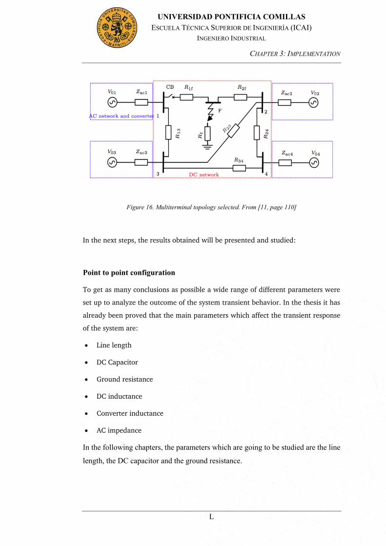
CHAPTER 3: IMPLEMENTATION
L
UNIVERSIDAD PONTIFICIA COMILLAS ESCUELA TÉCNICA SUPERIOR DE INGENIERÍA (ICAI)
INGENIERO INDUSTRIAL
Figure 16. Multiterminal topology selected. From [11, page 110]
In the next steps, the results obtained will be presented and studied:
Point to point configuration
To get as many conclusions as possible a wide range of different parameters were
set up to analyze the outcome of the system transient behavior. In the thesis it has
already been proved that the main parameters which affect the transient response
of the system are:
x Line length
x DC Capacitor
x Ground resistance
x DC inductance
x Converter inductance
x AC impedance
In the following chapters, the parameters which are going to be studied are the line
length, the DC capacitor and the ground resistance.
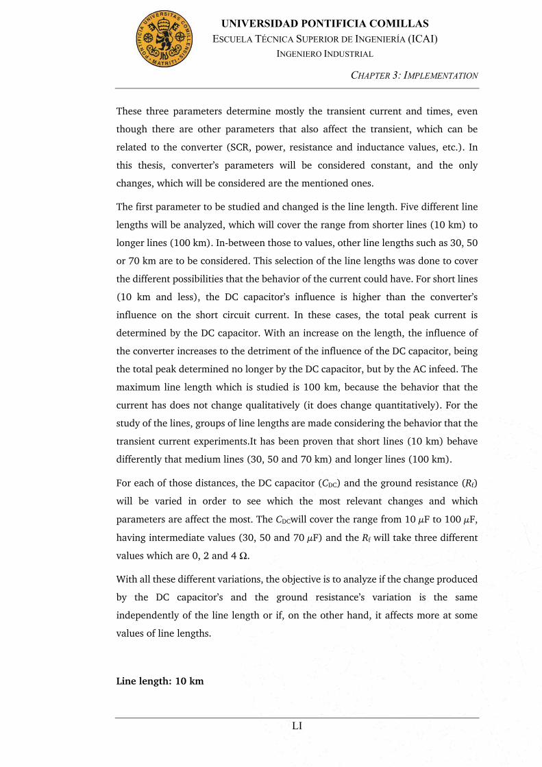
CHAPTER 3: IMPLEMENTATION
LI
UNIVERSIDAD PONTIFICIA COMILLAS ESCUELA TÉCNICA SUPERIOR DE INGENIERÍA (ICAI)
INGENIERO INDUSTRIAL
These three parameters determine mostly the transient current and times, even
though there are other parameters that also affect the transient, which can be
related to the converter (SCR, power, resistance and inductance values, etc.). In
this thesis, converter’s parameters will be considered constant, and the only
changes, which will be considered are the mentioned ones.
The first parameter to be studied and changed is the line length. Five different line
lengths will be analyzed, which will cover the range from shorter lines (10 km) to
longer lines (100 km). In-between those to values, other line lengths such as 30, 50
or 70 km are to be considered. This selection of the line lengths was done to cover
the different possibilities that the behavior of the current could have. For short lines
(10 km and less), the DC capacitor’s influence is higher than the converter’s
influence on the short circuit current. In these cases, the total peak current is
determined by the DC capacitor. With an increase on the length, the influence of
the converter increases to the detriment of the influence of the DC capacitor, being
the total peak determined no longer by the DC capacitor, but by the AC infeed. The
maximum line length which is studied is 100 km, because the behavior that the
current has does not change qualitatively (it does change quantitatively). For the
study of the lines, groups of line lengths are made considering the behavior that the
transient current experiments.It has been proven that short lines (10 km) behave
differently that medium lines (30, 50 and 70 km) and longer lines (100 km).
For each of those distances, the DC capacitor (CDC) and the ground resistance (Rf)
will be varied in order to see which the most relevant changes and which
parameters are affect the most. The CDCwill cover the range from 10 µF to 100 µF,
having intermediate values (30, 50 and 70 µF) and the Rf will take three different
values which are 0, 2 and 4 Ω.
With all these different variations, the objective is to analyze if the change produced
by the DC capacitor’s and the ground resistance’s variation is the same
independently of the line length or if, on the other hand, it affects more at some
values of line lengths.
Line length: 10 km
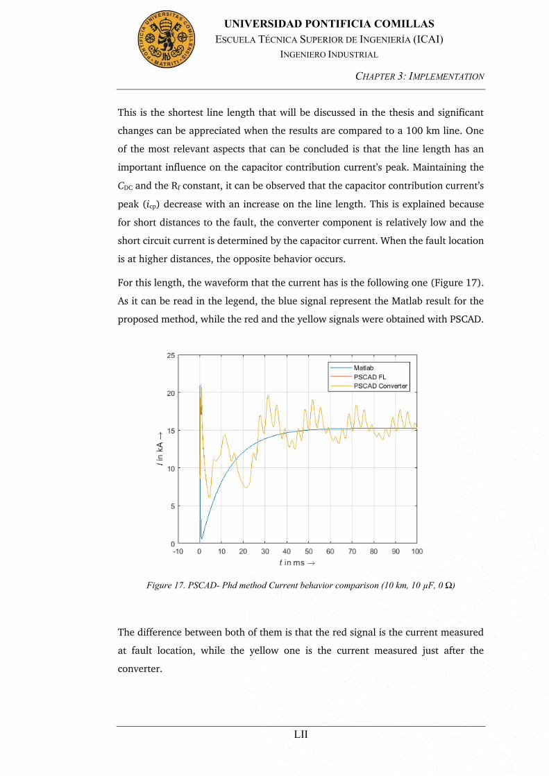
CHAPTER 3: IMPLEMENTATION
LII
UNIVERSIDAD PONTIFICIA COMILLAS ESCUELA TÉCNICA SUPERIOR DE INGENIERÍA (ICAI)
INGENIERO INDUSTRIAL
This is the shortest line length that will be discussed in the thesis and significant
changes can be appreciated when the results are compared to a 100 km line. One
of the most relevant aspects that can be concluded is that the line length has an
important influence on the capacitor contribution current’s peak. Maintaining the
CDC and the Rf constant, it can be observed that the capacitor contribution current’s
peak (icp) decrease with an increase on the line length. This is explained because
for short distances to the fault, the converter component is relatively low and the
short circuit current is determined by the capacitor current. When the fault location
is at higher distances, the opposite behavior occurs.
For this length, the waveform that the current has is the following one (Figure 17).
As it can be read in the legend, the blue signal represent the Matlab result for the
proposed method, while the red and the yellow signals were obtained with PSCAD.
Figure 17. PSCAD- Phd method Current behavior comparison (10 km, 10 µF, 0 Ω)
The difference between both of them is that the red signal is the current measured
at fault location, while the yellow one is the current measured just after the
converter.

CHAPTER 3: IMPLEMENTATION
LIII
UNIVERSIDAD PONTIFICIA COMILLAS ESCUELA TÉCNICA SUPERIOR DE INGENIERÍA (ICAI)
INGENIERO INDUSTRIAL
Even though the difference is almost not appreciated, the PhD method was
developed for the current after the converter and the TUD dissertation was
developed for the current at fault location.
As it was said before, for shorter lines, the DC capacitor has more influence than for
longer lines, and in this case, the total peak current of the transient (ip) matches
with the capacitor contribution current’s peak (icp).
The next step is to analyze how the behavior changes for alterations in the CDC and
the Rf.
First, the Rf will be kept constant to a certain value (0 Ω for example), and the
relative and absolute error in the peak and steady state current will be measured
for different values of the CDC. Afterwards, the procedure will be done the other way
around, keeping constant the DC capacitor and making variations in the ground
resistance. In this figure Figure 18, the absolute error for the PhD method can be
seen for different values of CDC, when the Rf is kept constant.
Figure 18. Absolute error for PTP x = 10 km,Rf = 0 Ω and variation in CDC

CHAPTER 3: IMPLEMENTATION
LIV
UNIVERSIDAD PONTIFICIA COMILLAS ESCUELA TÉCNICA SUPERIOR DE INGENIERÍA (ICAI)
INGENIERO INDUSTRIAL
Errors from three different points are measured (capacitor contribution current
peak (icp), total current peak (ip) and steady state current (Ik)). These points are
taken and measured from the time course current that the equations provide.
Analyzing the three different characteristic points, it is interesting to see, how Ik
does not experiment any variation when the CDC is modified. As it was explained
before, this is because the CDC has its influence in the first part of the transient, and
not in the last part, when the steady state current is determined. In the next
chapters, it will be seen how this steady state current varies depending on the line
length and the ground resistance, but remains unchanged for different values of
CDC. This is explained, due to the fact that the contribution of the CDC is extinguished
in the last part of the transient, where the steady state current is determined. For
the exposed configuration, the absolute error is lower than 0.1 kA.
Another interesting point to see, is that for short lines, the peak current matches
with the capacitor contribution’s peak.
This current peak’s error reaches its minimum value for very low capacitors, being
almost 0 for 10 µF. An increase in this value, makes the error increase, reaching its
maximum value for 100 µF, 0.5 kA.
CHAPTER 3: IMPLEMENTATION
LV
UNIVERSIDAD PONTIFICIA COMILLAS ESCUELA TÉCNICA SUPERIOR DE INGENIERÍA (ICAI)
INGENIERO INDUSTRIAL
In the next figure (Figure 19), the relative error for the PhD method can be seen for
different values of CDC, when the Rf is kept constant.
Figure 19. Relative error for PTP x = 10 km, Rf = 0 Ωand variation in CDC
It is also important to check the errors in a relative way, due to the fact that an error
of 1 kA is not equally critical when the expected value is 2 kA or 20 kA. In the case
of PTP configurations, for a 10 km line and ground resistance of 0 Ω, the relative
error for the peak current varies between almost 0 %, for low DC capacitors, and -
2.5 % for the highest DC capacitors. Taking a look at the steady state current, the
relative error is slightly below 0.5% for all the values of CDC.
The next figures (Figure 20 and Figure 22) will show the absolute and relative error
for steady state, and peak current in a configuration where the CDC remains
unchanged (10 µF) and the Rf changes from 0 to 4 Ω.
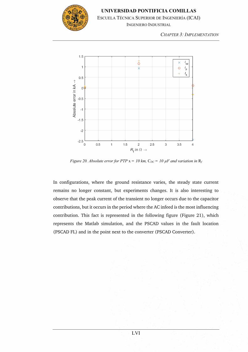
CHAPTER 3: IMPLEMENTATION
LVI
UNIVERSIDAD PONTIFICIA COMILLAS ESCUELA TÉCNICA SUPERIOR DE INGENIERÍA (ICAI)
INGENIERO INDUSTRIAL
Figure 20. Absolute error for PTP x = 10 km, CDC = 10 µF and variation in Rf
In configurations, where the ground resistance varies, the steady state current
remains no longer constant, but experiments changes. It is also interesting to
observe that the peak current of the transient no longer occurs due to the capacitor
contributions, but it occurs in the period where the AC infeed is the most influencing
contribution. This fact is represented in the following figure (Figure 21), which
represents the Matlab simulation, and the PSCAD values in the fault location
(PSCAD FL) and in the point next to the converter (PSCAD Converter).
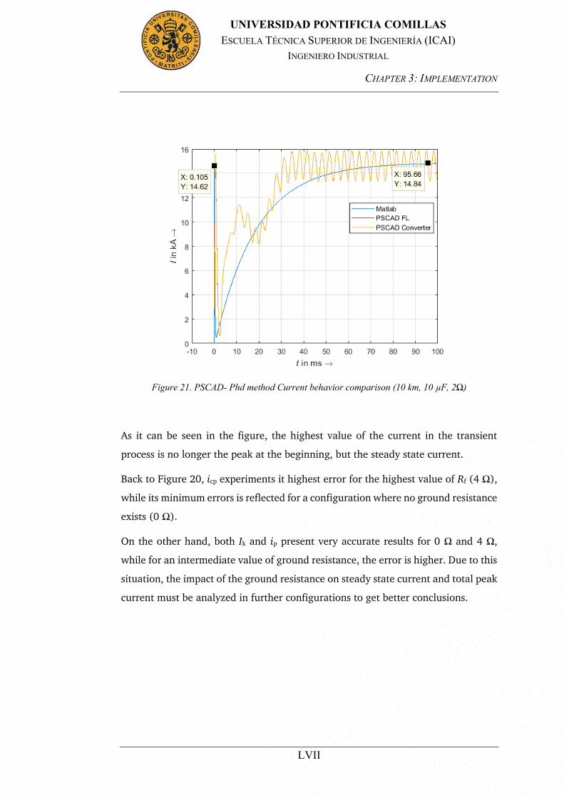
CHAPTER 3: IMPLEMENTATION
LVII
UNIVERSIDAD PONTIFICIA COMILLAS ESCUELA TÉCNICA SUPERIOR DE INGENIERÍA (ICAI)
INGENIERO INDUSTRIAL
Figure 21. PSCAD- Phd method Current behavior comparison (10 km, 10 µF, 2Ω)
As it can be seen in the figure, the highest value of the current in the transient
process is no longer the peak at the beginning, but the steady state current.
Back to Figure 20, icp experiments it highest error for the highest value of Rf (4 Ω),
while its minimum errors is reflected for a configuration where no ground resistance
exists (0 Ω).
On the other hand, both Ik and ip present very accurate results for 0 Ω and 4 Ω,
while for an intermediate value of ground resistance, the error is higher. Due to this
situation, the impact of the ground resistance on steady state current and total peak
current must be analyzed in further configurations to get better conclusions.
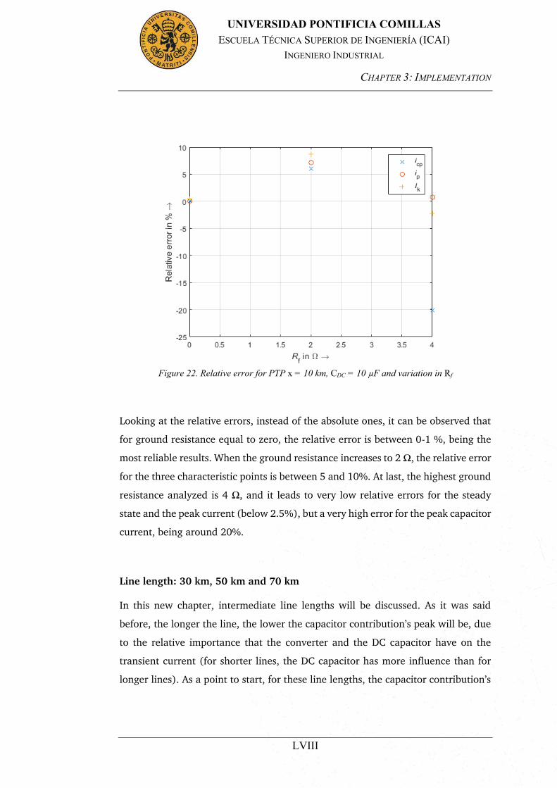
CHAPTER 3: IMPLEMENTATION
LVIII
UNIVERSIDAD PONTIFICIA COMILLAS ESCUELA TÉCNICA SUPERIOR DE INGENIERÍA (ICAI)
INGENIERO INDUSTRIAL
Figure 22. Relative error for PTP x = 10 km, CDC = 10 µF and variation in Rf
Looking at the relative errors, instead of the absolute ones, it can be observed that
for ground resistance equal to zero, the relative error is between 0-1 %, being the
most reliable results. When the ground resistance increases to 2 Ω, the relative error
for the three characteristic points is between 5 and 10%. At last, the highest ground
resistance analyzed is 4 Ω, and it leads to very low relative errors for the steady
state and the peak current (below 2.5%), but a very high error for the peak capacitor
current, being around 20%.
Line length: 30 km, 50 km and 70 km
In this new chapter, intermediate line lengths will be discussed. As it was said
before, the longer the line, the lower the capacitor contribution’s peak will be, due
to the relative importance that the converter and the DC capacitor have on the
transient current (for shorter lines, the DC capacitor has more influence than for
longer lines). As a point to start, for these line lengths, the capacitor contribution’s

CHAPTER 3: IMPLEMENTATION
LIX
UNIVERSIDAD PONTIFICIA COMILLAS ESCUELA TÉCNICA SUPERIOR DE INGENIERÍA (ICAI)
INGENIERO INDUSTRIAL
peak will no longer match with the total peak of the transient period. In these cases,
the global peak of the current will be due to the AC infeed.
In the appendix, Figure 42 and Figure 43 show the time domain signals for 30 km
and 70 km (CDC = 10 µF and Rf = 0 Ω).
It is important to check if the changes of the parameters (CDC and Rf) affect in the
same way to medium line lengths systems than to short line lengths systems. To do
so, the same procedure will be followed, maintaining in one case the CDC constant
and applying changes to Rf, and in the other case the other way around.
The variables to study are the same ones that were studied before: peak currents
(both contributions) and steady state current. Results from the three line lengths
were obtained and it can be said that the system behaves the same for the different
line lengths, so it makes sense to make an aggrupation of medium lines for the
analysis.
As it was done before, first the ground resistance will be set to a certain value (0 Ω)
and it will be kept constant. It is observed that a change in the DC capacitor does
not have much influence in the % of error that the method presents. There are very
few variations between different values of CDC in the three of the variables. These
figures can be seen in the appendix Figure 44 and Figure 45.
ip remains unchanged for the different values of CDC This is because the total peak
of the system occurs once the capacitor contribution is extinguished and the dc
capacitor does not have any influence.
When looking at ipc, the error that it presents is practically constant, but experiments
a slight tendency to increase the error, as the value of the DC capacitor increases.
The steady state current error is also constant, for the same reason that the total
peak current remains unchanged.
To sum up, the steady state and the peak current errors remain unchanged when
the CDC is changed, while the capacitor contribution current peak’s error slightly
presents a tendency to increase with an increase in the CDC.

CHAPTER 3: IMPLEMENTATION
LX
UNIVERSIDAD PONTIFICIA COMILLAS ESCUELA TÉCNICA SUPERIOR DE INGENIERÍA (ICAI)
INGENIERO INDUSTRIAL
Now, the ground resistance will be the changing parameter, while the CDC remains
constant. The Figure 46 and Figure 47 are attached in the appendix.
For these analysis, it is helpful to analyze each of the characteristic points of the
current in an independent way, as a change in Rf does not have the same influence
in the total peak current, the steady state or capacitor contribution’s peak current.
First, the steady state current will be studied. Contrary to the previous change in
the DC capacitor, the ground resistance does have big influence on the steady state
current. Even though, the value of the steady state current changes with a variation
of the ground resistance, the relative error of this characteristic point of the current
remains always very low, increasing slightly with an increase in the ground
resistance.
When the characteristic value studied is icp, the system does not behave in a linear
way, and no clear tendency can be obtained. The only aspect that is repeated
constantly for the different line lengths is that the method usually overestimates the
value for low and high values of ground resistance and underestimates the peak for
intermediate values of ground resistance.
Finally, the total peak value of the current experiments better results for higher
values of ground resistance.
Line length: 100 km
The longest line lengths analyzed are the 100 km ones. In these lines, the difference
of the capacitor contribution’s peak and the peak of the ac infeed is the highest in
the studied cases. The following picture (Figure 23) will show the PSCAD time
waves from a 10 km and a 100 km line length superposed.
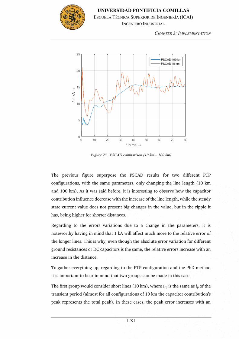
CHAPTER 3: IMPLEMENTATION
LXI
UNIVERSIDAD PONTIFICIA COMILLAS ESCUELA TÉCNICA SUPERIOR DE INGENIERÍA (ICAI)
INGENIERO INDUSTRIAL
Figure 23 . PSCAD comparison (10 km – 100 km)
The previous figure superpose the PSCAD results for two different PTP
configurations, with the same parameters, only changing the line length (10 km
and 100 km). As it was said before, it is interesting to observe how the capacitor
contribution influence decrease with the increase of the line length, while the steady
state current value does not present big changes in the value, but in the ripple it
has, being higher for shorter distances.
Regarding to the errors variations due to a change in the parameters, it is
noteworthy having in mind that 1 kA will affect much more to the relative error of
the longer lines. This is why, even though the absolute error variation for different
ground resistances or DC capacitors is the same, the relative errors increase with an
increase in the distance.
To gather everything up, regarding to the PTP configuration and the PhD method
it is important to bear in mind that two groups can be made in this case.
The first group would consider short lines (10 km), where icp is the same as ip of the
transient period (almost for all configurations of 10 km the capacitor contribution’s
peak represents the total peak). In these cases, the peak error increases with an

CHAPTER 3: IMPLEMENTATION
LXII
UNIVERSIDAD PONTIFICIA COMILLAS ESCUELA TÉCNICA SUPERIOR DE INGENIERÍA (ICAI)
INGENIERO INDUSTRIAL
increase of the DC capacitor, while it does not behave in a uniform way with a
change in the ground resistance. Hence, no reliable conclusions can be obtained for
a change in the ground resistance. On the other hand, the steady state current
presents no change against variations in the DC capacitor, and it presents very good
results for low and high values of ground resistance, being slightly worse for
intermediate values.
The second group would be the configurations where the capacitor’s peak does not
represent the total current’s peak. Some configurations of 10 km line lengths and
the totality of longer lines belong to this group. For this group, three different
characteristic points must be taken into account. First, the steady state current’s
estimation deteriorates with increasing values of ground resistance, while it remains
unchanged for different values of DC capacitor. Secondly, the total peak current’s
error decreases with an increase in the value of ground resistance and remains
unchanged for different values of DC capacitor (as when the total peak occurs, the
influence of the capacitive sources is already extinguished). Finally, the current’s
capacitor current does not present clear results in order to achieve a good
conclusion. It is noticeable that it tends to underestimate the real value for low and
high ground resistance’s values and to overestimate for intermediate values.
The last analysist that will be done for this method in the PTP configurations will
be regarding to the line lengths. To do so, ground resistance’s and dc capacitor’s
values will be kept constant (10 µF and 0 Ω). The results can be seen in the appendix
in Figure 48 and Figure 49.
Analyzing the three different characteristic points for different distances interesting
conclusions can be taken.
The behavior of the steady state current is very good, remaining the relative error
for the five distances below 2%. There is a slight tendency for this error to increase
with the distance.
The total peak estimations present its minimum value for 10 km, where this peak is
the same as the capacitor’s contribution peak current. If this value is omitted, the
error decreases with an increase of the distance, being in all cases the value
overestimated.
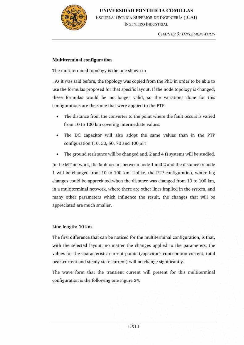
CHAPTER 3: IMPLEMENTATION
LXIII
UNIVERSIDAD PONTIFICIA COMILLAS ESCUELA TÉCNICA SUPERIOR DE INGENIERÍA (ICAI)
INGENIERO INDUSTRIAL
Multiterminal configuration
The multiterminal topology is the one shown in
. As it was said before, the topology was copied from the PhD in order to be able to
use the formulas proposed for that specific layout. If the node topology is changed,
these formulas would be no longer valid, so the variations done for this
configurations are the same that were applied to the PTP:
x The distance from the converter to the point where the fault occurs is varied
from 10 to 100 km covering intermediate values.
x The DC capacitor will also adopt the same values than in the PTP
configuration (10, 30, 50, 70 and 100 µF)
x The ground resistance will be changed and, 2 and 4 Ω systems will be studied.
In the MT network, the fault occurs between node 1 and 2 and the distance to node
1 will be changed from 10 to 100 km. Unlike, the PTP configuration, where big
changes could be appreciated when the distance was changed from 10 to 100 km,
in a multiterminal network, where there are other lines implied in the system, and
many other parameters which influence the result, the changes that will be
appreciated are much smaller.
Line length: 10 km
The first difference that can be noticed for the multiterminal configuration, is that,
with the selected layout, no matter the changes applied to the parameters, the
values for the characteristic current points (capacitor’s contribution current, total
peak current and steady state current) will no change significantly.
The wave form that the transient current will present for this multiterminal
configuration is the following one Figure 24:
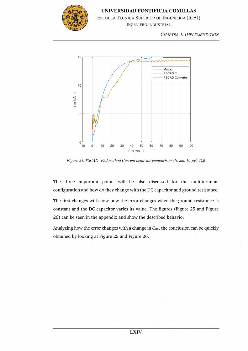
CHAPTER 3: IMPLEMENTATION
LXIV
UNIVERSIDAD PONTIFICIA COMILLAS ESCUELA TÉCNICA SUPERIOR DE INGENIERÍA (ICAI)
INGENIERO INDUSTRIAL
Figure 24. PSCAD- Phd method Current behavior comparison (10 km, 10 µF, 2Ω)
The three important points will be also discussed for the multiterminal
configuration and how do they change with the DC capacitor and ground resistance.
The first changes will show how the error changes when the ground resistance is
constant and the DC capacitor varies its value. The figures (Figure 25 and Figure
26) can be seen in the appendix and show the described behavior.
Analyzing how the error changes with a change in CDC, the conclusion can be quickly
obtained by looking at Figure 25 and Figure 26.

CHAPTER 3: IMPLEMENTATION
LXV
UNIVERSIDAD PONTIFICIA COMILLAS ESCUELA TÉCNICA SUPERIOR DE INGENIERÍA (ICAI)
INGENIERO INDUSTRIAL
Figure 25. Absolute error for MT x = 10 km, Rf = 2 Ω and variation in CDC
Figure 26. Relative error for MT x = 10 km, Rf = 2 Ω and variation in CDC

CHAPTER 3: IMPLEMENTATION
LXVI
UNIVERSIDAD PONTIFICIA COMILLAS ESCUELA TÉCNICA SUPERIOR DE INGENIERÍA (ICAI)
INGENIERO INDUSTRIAL
In this case, the DC capacitor does not have any influence on the presented error
and it remains practically unchanged. In the steady state current and peak current,
in fact, it does not change at all, due to the fact that the DC capacitor has an
influence in the first part of the transient and then it extinguishes. Once the
influence of the DC capacitor is extinguished, the AC infeed is the one that
determines the value of total peak and steady state current. The capacitor current’s
peak presents slight changes, with differences lower than 0.5%.
Once the influence of the DC capacitor is tested, the ground resistance is the
parameter to look at. CDC will be set to 10 µF and Rf will change in order to try to
find a tendency in the way the method works for different values of resistances.
The figures (Figure 50 and Figure 51) show the absolute and relative error that the
system has when the ground resistance is changed. As it can be seen, the capacitor
current contribution’s peak error and the steady state current’s error is not affected
by a change in the resistance, while the peak of the system’s error does change. In
this case, the error increases by almost 1%.
Line length: 30, 50 and 70 km
The next line lengths to be analyzed are the medium lines. For these lines, the
behavior against a change in the DC capacitor is the same as for short lines (10 km).
If the parameter kept constant is the CDC and the Rf changes, the behavior of the icp
is the same that the one seen in short lines. On the other hand, Ik and ip error have
a different variation when analyzing medium lines. To do the analysis, the following
figures will be useful. The results are in the appendix (Figure 52 and Figure 53)
The conclusion that can be obtained from the data taken is that the method tends
to underestimate the values for lower ground resistances and overestimate for
higher values of ground resistance, being the error very low in both cases and below
4%.

CHAPTER 3: IMPLEMENTATION
LXVII
UNIVERSIDAD PONTIFICIA COMILLAS ESCUELA TÉCNICA SUPERIOR DE INGENIERÍA (ICAI)
INGENIERO INDUSTRIAL
Line length: 100 km
The estimations for long line lengths present the same error variation that medium
line lengths.
The last analysis to do for multiterminal configurations is how the distance to fault
affects the current estimations. For it, the DC capacitor and the ground resistance
will be set to 10 µF and 2 Ω respectively. The figures can be seen in the appendix
(Figure 54 and Figure 55)
For the steady state current, the best results are obtained for short distances (less
than 0.5% of relative error), while for medium and long lines the error stabilizes in
3.5%.
When the point to be studied is the total peak current, it can be seen how the error
is also slightly better for short lines (around 0.5% better) than for medium and long
lines.
To finish with the characteristic points, the capacitor current contribution’s peak is
the only value which presents worse results for short than for medium and long
lines. In this case, the difference is higher than before, and it is of almost 4% worse
for short lines.
Knowing how the three values change and where does these currents come from, it
can be concluded that the capacitor contributions lead to better results in medium
and long lines, while the AC infeed contribution has slightly better estimations for
longer lines.
Conclusion
Once the influence of the parameters has been studied (both in PTP configurations
and MT networks, an explanation to the errors in the steady state current and in the
peak currents is provided.
The differences observed for the steady state current are due to the simplified
calculations that have been used. In these calculations, only the sixth harmonic was
considered, and not the rest of the harmonics which are present in the simulations.
CHAPTER 3: IMPLEMENTATION
LXVIII
UNIVERSIDAD PONTIFICIA COMILLAS ESCUELA TÉCNICA SUPERIOR DE INGENIERÍA (ICAI)
INGENIERO INDUSTRIAL
On the other hand, the error which is observed on the peak values are due to the
estimations errors in the single terminal damping ratio (ςT1). The value of the single
terminal damping ratio is estimated in the first place. This estimation leads to error
in the peak currents.
After these four steps, the PhD equations are totally executed, and the results are
ready to be compared with the TUD Dissertation method.
TUD DISSERTATION’S METHOD
This second method to study the system behavior was developed in TU Darmstadt
in 2016. Unlike the first method already discussed, this one does not provide a time
domain signal, but it gives some key values in the current response to a phase to
ground fault. These values are:
x Time to peak
x Steady state short circuit current
x Peak short circuit current
x Short circuit current initial slope
The given values correspond to the values experimented by the total current, taking
into account all the superpositions.
The work methodology applied to this method will be the same one applied to the
first one, and will be the following one:
x Equations implementation
x Checking the reliability of the formulas with PSCAD simulations
In this case, unlike the first method, the equations provided are directly considering
all the superposition of the different contributions (capacitive and AC infeed
contributions) and that step can be skipped.

CHAPTER 3: IMPLEMENTATION
LXIX
UNIVERSIDAD PONTIFICIA COMILLAS ESCUELA TÉCNICA SUPERIOR DE INGENIERÍA (ICAI)
INGENIERO INDUSTRIAL
To proceed in that way, the benchmark and the parameters selections proposed in
the dissertation will be taken and used for the Matlab simulations.
As it was said before, the aim of this part of the thesis is to be sure to implement
the formulas correctly, so that the results can be treated with a high level of
reliability. To do so, all the given parameters combinations will be tested and
compared.
As happened with the PhD from Zurich, the input parameters in these formulas are
the AC and DC impedances, the converter parameters and the voltages of the
system.
Two of the most important relations that are observed to have a big influence on
the output are the RDC and RAC relation, as well as La and LAC relation. With different
values for these relations, diverse output signals are observed, and the robustness
of the equations are tested. There can be big difference between a very low and a
very high parameter’s relation.
To be sure that the equations proposed in the dissertation were correct and that the
implementation done in Matlab was also satisfactory, these equations are
implemented in Matlab and the results are compared to the expected ones.
The original dissertation provides a wide range of parameters and its respective
results of steady state current, peak current, initial slope and time to peak. By
adopting the same parameters choice, the results obtained should be the same. By
doing this test, it can be proven that the equations are correct and the
implementation in Matlab is also adequate. Once this step is done, the parameters
selection can be changed and other conditions can be studied.
The comparison lead to some interesting results. The results obtained for the
characteristic points were accurate and in very few cases the results were slightly
different. Not even for the highest error, the difference was so big, that the
implementation could be categorized as wrong.
Once the formulas are implemented and compared to the proposed graphics of the
original publication, it can be said that the implementation of this publications is
CHAPTER 3: IMPLEMENTATION
LXX
UNIVERSIDAD PONTIFICIA COMILLAS ESCUELA TÉCNICA SUPERIOR DE INGENIERÍA (ICAI)
INGENIERO INDUSTRIAL
also completed. The next step is the comparison to PSCAD simulations in different
situations.
Comparison with PSCAD simulations
For the TU Darmstadt Dissertation method, also two different topologies were
studied. First, PTP configurations will be studied. The range of variations in the
parameters is the same that it was applied in the previous method.
A distinction between line lengths is done, where the distances simulated are 10,
30, 50, 70 and 100 km. The parameters which affect the behavior of the system are
the same (CDC and Rf). For each distance, five different values of DC capacitor (10,
30, 50, 70 and 100 µF) and three different values of ground resistance (0, 2 and 4
Ω ) values are tested.
Once the PTP configuration is studied and analyzed, the next topology is a
multiterminal network. In this case, the topology which will be adopted is the one
that was used for the PhD method and it can be seen in
. By making this decision, a comparison for the same configurations and topology
is possible between the two methods. The changes that will be applied to the
topology are related to the distance from the converter to the point where the fault
occur, the DC capacitor value and the ground resistance value.
Point to point configuration
Line length: 10 km
The first line length to analyze is 10 km, which will be the shortest distance to be
taken into account. With this line length, if the ground resistance is 0 Ω, the
capacitor’s current peak will be the total peak of the transient system. For higher
values of ground resistance, the peak current of the AC infeed contribution is
slightly higher. This aspect will be noticed in the following figures (Figure 27).

CHAPTER 3: IMPLEMENTATION
LXXI
UNIVERSIDAD PONTIFICIA COMILLAS ESCUELA TÉCNICA SUPERIOR DE INGENIERÍA (ICAI)
INGENIERO INDUSTRIAL
To analyze as deeply as possible how the variations affect the result, the process
will be separated in two parts. First, Rf will be kept constant, and CDC will change
between five different values (10, 30, 50, 70 and 100 µF). Afterwards, the DC
capacitor will be the parameter set to a fixed value and the ground resistance
changes. The relative error will be represented in Figure 27.
Figure 27. Relative error for PTP x = 10 km, Rf = 0 Ωand variation in CDC
Looking at the relative error of the three characteristic points of the current it can
be said that the results obtained are consistent for a value of ground resistance equal
to zero. The highest recorded error is below 6%, which matches with the expected
error for this method. The original publication [14]does not show the errors for this
exact parameter set-up, and uses other parameters. The results obtained with
similar parameters are comparable to ones showed in the thesis.
The DC capacitor does not have an influence in the steady state current, thus the
error remains constant, and below 0.5%. On the other hand, CDC has a big influence
on the peak values, especially in this situation where the capacitor contribution’s
peak is also the total peak of the current. Unfortunately, the error does not present
any tendency for the capacitor change, and it varies between -2% and 6% for the
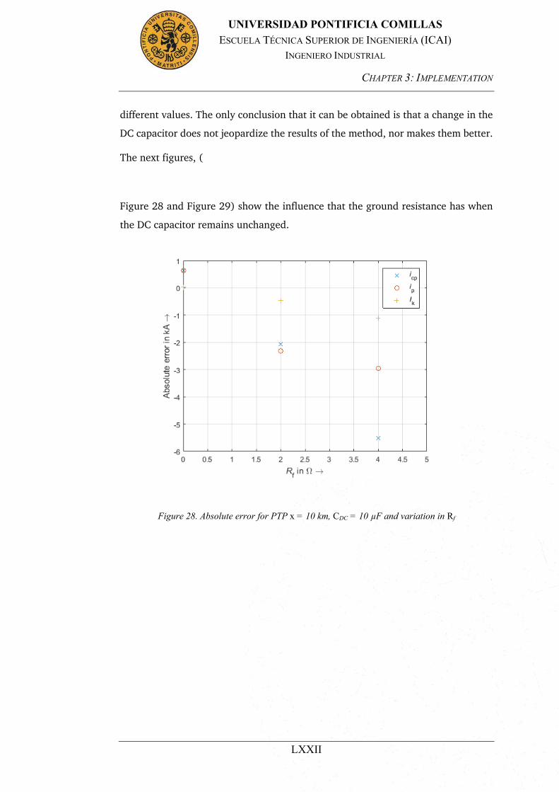
CHAPTER 3: IMPLEMENTATION
LXXII
UNIVERSIDAD PONTIFICIA COMILLAS ESCUELA TÉCNICA SUPERIOR DE INGENIERÍA (ICAI)
INGENIERO INDUSTRIAL
different values. The only conclusion that it can be obtained is that a change in the
DC capacitor does not jeopardize the results of the method, nor makes them better.
The next figures, (
Figure 28 and Figure 29) show the influence that the ground resistance has when
the DC capacitor remains unchanged.
Figure 28. Absolute error for PTP x = 10 km, CDC = 10 µF and variation in Rf

CHAPTER 3: IMPLEMENTATION
LXXIII
UNIVERSIDAD PONTIFICIA COMILLAS ESCUELA TÉCNICA SUPERIOR DE INGENIERÍA (ICAI)
INGENIERO INDUSTRIAL
Figure 29. Relative error for PTP x = 10 km, CDC = 10 µF and variation in Rf
When the parameter to be modified is Rf, the tendency shown in the values is clear
and in the three cases an increase in the ground resistance imply an increase in the
error made. The most affected point is the capacitor contribution’s peak, whose
error reaches around 45 % for a ground resistance of 4 Ω. The total peak current is
also affected by an increase in the ground resistance and its error reaches 20% at
its maximum. The steady state current is the less affected point, being its error
always below 10%.
Line length: 30, 50 and 70 km
The methodology to follow in intermediate line lengths is the same as the one
followed for shorter lines. First, the ground resistance will be set to a certain value
(0 Ω) and the DC capacitor will adopt different values (10, 30, 50, 70 and 100 µF).
Once, the influence of the capacitor is studied, the ground resistance will be the
parameter that changes. It is also very important to check if the behavior observed
for the different line length is the same or not.

CHAPTER 3: IMPLEMENTATION
LXXIV
UNIVERSIDAD PONTIFICIA COMILLAS ESCUELA TÉCNICA SUPERIOR DE INGENIERÍA (ICAI)
INGENIERO INDUSTRIAL
For a ground resistance set to 0 Ω, it is safe to assure that the change in the DC
capacitor affects the same way all the line lengths (30, 50 and 70 km). In this case,
no significant change is appreciated for any of the distances and values of the DC
capacitor. The error for the three characteristic current’s points remains unchanged.
The figures attached in the appendix (Figure 56 and Figure 57) will serve as an
example for the intermediate line lengths. It represents a 50 km line length, which
qualitatively has the same behavior as the 30 and 70 km lines.
When the parameter changed is the ground resistance, the errors vary much more
than before. That is to say, a ground resistance variation makes the method much
more vulnerable than a DC capacitor variation. The results can be seen in the
appendix (Figure 58 and Figure 59).
As it was said before, prior to reach to any conclusion for intermediate line lengths,
it is important to see if a change in the ground resistance affects the same way every
line in this group. This aspect was checked and it is confirmed that the three line
lengths react the same way to changes in the ground resistance.
First, the steady state current is examined. This is the value that has less variation,
and the maximum variation for extreme values is around 5%. Further, higher values
of Rf increase the error in the estimated value.
The capacitor contribution’s peak also experiments big changes for different values
of ground resistance and has better performance for intermediate than for extreme
values.
The last value to look at, is the total peak current, whose tendency is the same as
the steady state current. The best performance comes when the ground resistance
is zero, while an increase in the resistance makes the result worse. An increase of 4
Ω can affect around 10% in the final result.
Line length: 100 km
For long lines, the behavior that is observed is similar than for intermediate line
lengths, with slight differences.

CHAPTER 3: IMPLEMENTATION
LXXV
UNIVERSIDAD PONTIFICIA COMILLAS ESCUELA TÉCNICA SUPERIOR DE INGENIERÍA (ICAI)
INGENIERO INDUSTRIAL
First, the influence of a variation in the DC capacitor is studied, remaining the
ground resistance fixed to 0 Ω. As it happened with intermediate lines, CDC has
almost no influence in the error variation in none of the current characteristic
points. Even though, the values change, the error that the system presents are
constant when it is compared to PSCAD simulations.
The second parameter to change its value is the ground resistance. As happened
before, when Rf varies, the method behaves better for certain situations.
The only difference in this point is in Ik. For this length of line, the steady state
current’s estimation improves its performance with an increase in the ground
resistance, while for short and medium lines it was the other way around. The peak
currents vary the same way that they did for medium lines.
Once the influence of the different parameters is tested for short, medium and long
lines, the last point to test for PTP configurations is compare how does the error
react to different line lengths when the same parameters are set to the system. The
parameters, which will be used for the comparison are 10 µF and 0 Ω. The figures
attached in the appendix (Figure 60 and ) will show the absolute and relative error
measured for the different lengths.
This is one of the most important analysis that will be done, as it can be compared
the performance of the method for different line lengths. It is very important to
check the method’s robustness. A good method will not present a lot of differences
between shorter and longer distances.
In the figures in the appendix, (Figure 60 and ) it can be observed that the error
does not vary much from the shortest distance to the longest one. The maximum
variation experimented is around 5%, which in absolute value represent less than
1 kA. Taking a deeper look and analyzing the three different characteristic points,
three different behaviors are observed.
First, the steady state current has its better results for short lines, increasing the
error for intermediate and long lines. In all the cases, the recorded relative error is
below 5%.

CHAPTER 3: IMPLEMENTATION
LXXVI
UNIVERSIDAD PONTIFICIA COMILLAS ESCUELA TÉCNICA SUPERIOR DE INGENIERÍA (ICAI)
INGENIERO INDUSTRIAL
The total peak current’s performance is different and reaches relative errors below
1% for intermediate distances, while this error increases both for short and long
lines, being the maximum error 3%.
Last, the capacitor’s current does not present a clear tendency in the presented
error. When the capacitor current peak matches with the peak current, the error
reaches its minimum value (3%), but when this peak no longer represent the total
peak of the transient period, the relative error can reach values of almost 12 %. The
only conclusion that can be extracted from these analysis is that for short lines,
when the peak represents the total peak of the transient period the estimated value
is much better than for longer lines, when this peak is only a relative maximum and
not the absolute.
Multiterminal configuration
The next step is to check if the results present the same grade of accuracy when
more nodes are added into the system. The multiterminal network which is going
to be tested is the same one that it was used for the PhD method. This configuration
is adopted for the same reasons given before and also to be able to compare both
methods afterwards and observe which one presents better results in the different
situations.
The parameters which are going to be changed for this configurations are: the
distance to the fault location from the converter, the value of the DC capacitor and
the ground resistance. The lines will be divided into three different groups: short
lines (10 km), intermediate lines (30, 50 and 70 km) and long lines (100 km).
Line length: 10 km
For the three groups of lines, the procedure to follow is the same as the one done
in the previous chapters. First, the ground resistance will be kept constant and the
influence of a variation in the DC capacitor in the absolute and relative error will
be studied. Later, the influence of the ground resistance will be one tested when the

CHAPTER 3: IMPLEMENTATION
LXXVII
UNIVERSIDAD PONTIFICIA COMILLAS ESCUELA TÉCNICA SUPERIOR DE INGENIERÍA (ICAI)
INGENIERO INDUSTRIAL
DC capacitor value is constant. The results when Rf is the fixed parameter and CDC
changes can be observed in the appendix (Figure 62 and ).
For short lines, it can be observed, how icp yields results which are not as good as it
can be expected. The error reaches its maximum for 10 µF and its stabilizes for
higher values of CDC in 40 %. On the other hand, Ik and ip does have better results,
being the best ones for the lowest capacitor value. As happened with icp, the error
stabilizes for the rest of the values of DC capacitor and does not present any further
variation.
By changing the ground resistance to other values, the results that are appreciated
are practically unchanged for steady state current and total peak current. On the
other hand, the capacitor current’s peak estimation’s performance changes and
improves by 10% for an increase to 4 Ω in the ground resistance.
Line length: 30, 50 and 70 km
For medium line lengths, the results of the system’s estimations against a change in
the CDC are practically the same than for short lines. In this case, the only difference
is that not even for values of DC capacitor of 10 µF, the error varies and it remains
unchanged regardless of what values does the DC capacitor take. This can be
observed in the figures attached in the appendix (Figure 64 and Figure 65).
The ground resistance value has more influence on the error variation than the DC
capacitor, but when comparing the changes to the PTP configuration, it can be
observed how in multiterminal networks there are many other parameters that
affect in the system stability and makes the system more robust against changes.
For that reason, a change in the ground resistance does not change as drastically
the error as it affected in the point to point configuration. Nevertheless, an increase
in the ground resistance improves the estimation accuracy of the total peak current.
The steady state current error remains unchanged and the capacitor current’s peak
error increases slightly.
All these changes can be checked in the figures attached in the appendix (Figure 66
and Figure 67), which represent a 50 km line length multiterminal configuration
with the DC capacitor set to 10 µF.

CHAPTER 3: IMPLEMENTATION
LXXVIII
UNIVERSIDAD PONTIFICIA COMILLAS ESCUELA TÉCNICA SUPERIOR DE INGENIERÍA (ICAI)
INGENIERO INDUSTRIAL
Line length: 100 km
The estimations for long line lengths present the same error variation that
intermediate line lengths.
To finish with the sensibility analysis for the different parameters that affect the
current behavior in the transient period when a fault occurs, the last parameter to
change is the distance to the fault location. The results for these changes can be
seen in the appendix (Figure 68 and Figure 69).
This last analysis is very interesting in order to check how good will be results be
depending on the line length. By first glance it can be seen how there is one
characteristic point which is very sensible to changes in the line length. This value
is the capacitor current’s peak, which also presents high sensibility to changes in the
ground resistance and the DC capacitor. It can be seen how for short and long lines,
the error is almost of 50%, while for intermediate values the error can reach values
of 10%.
The steady state current estimation’s performance does not present big alterations
when the distance to the fault changes, and remains for all the range of distances
below 2%, having accurate results.
The total peak current’s error also presents itself as robust against changes in the
distance and the error varies between 10% and 7% in extreme cases. It cannot be
concluded that a relation between distance and error exists.

CHAPTER 4: COMPARISON
LXXIX
UNIVERSIDAD PONTIFICIA COMILLAS ESCUELA TÉCNICA SUPERIOR DE INGENIERÍA (ICAI)
INGENIERO INDUSTRIAL
CHAPTER 4 : COMPARISON
In this step of the thesis, both methods have been satisfactory implemented in
Matlab and compared to the expected results according to their original thesis. A
sensibility test has also been done to the different configurations (both point to
point and multiterminal configurations from both methods).
The next step is the main objective of the thesis and consists of the comparison of
the performance of the different results when the configurations changes. The
results obtained from the sensibility analysis will be used and the comparison will
be done with the following approach:
A distinction between transmission networks will be done. The point to point
configuration will be the first one to be studied and afterwards the multiterminal
network will follow the same steps of the analysis.
For both point to point and multiterminal networks, groups of line lengths will be
done in relation to the previous behavior against changes in the parameters. These
groups will be: shorter lines (10 km), medium lines (30, 50 and 70 km) and longer
lines (100 km). For each one of this group lines, the steady state current, total peak
current and capacitor’s contribution peak current will be studied and the results
from PSCAD will be compared to the PhD’s and the TU Darmstadt’s methods.
For each one of the group lines, the DC capacitor, as well as the ground resistance
will be changed and the errors will be measured and compared.
POINT TO POINT CONFIGURATION
Line length: 10 km
The first case of study are short lines. The results for the steady state current are
very satisfactory for both methods.
In the first place, when the ground resistance is fixed, a change in the DC capacitor
does not vary the steady state current, so the error is the same. This happens for

CHAPTER 4: COMPARISON
LXXX
UNIVERSIDAD PONTIFICIA COMILLAS ESCUELA TÉCNICA SUPERIOR DE INGENIERÍA (ICAI)
INGENIERO INDUSTRIAL
every configuration, so from now on, the steady state current will only be studied
for changes in the ground resistance, as a change in the DC capacitor does not make
any sense in this case.
As discussed before, three different values of ground resistance were studied (0, 2
and 4 Ω). Having a look to all the results obtained for the different resistance values,
the TU Darmstadt method presents itself as a better method, obtaining errors of only
0.23 % for the lowest value of ground resistance. The main advantage of this
method is that the error changes in a linear way, knowing that for higher values of
resistance the error will always increase. It can be said that the method is more
predictable in its estimations.
The PhD method also presents good results having in some cases only 0.42% of
variation, but, on the other hand, it is more sensible to changes and a variation in
the resistance does not always affect in the same way, increasing the error up to
8.71 % for a value of 2 Ω and being reduced again to 2.28% when the resistance
acquires a value of 4 Ω.
The next values to be studied are the peak current. When studying these values,
both approaches present accurate results for ground resistances of 0 Ω, being all the
errors below 6 % for different DC capacitors. For that case, the PhD approach
presents outstanding results being below 3% in all cases and having a slightly better
performance. On the other hand, when the ground resistance increases its value,
none of the methods can be as reliable as they are for zero ground resistance. In an
extreme case of 4 Ω, the error for the total peak current is lower for the PhD method,
while the capacitor contribution peak’s estimation is better for the TUD
Dissertation.
As a conclusion for short lines it can be said the TU Darmstadt Dissertation’s
method presents better results for steady state current and capacitor’s current peak,
while the total peak current’s estimation is better for PhD method. It is noteworthy
to keep in mind that in any case the results of one of the methods were significantly
worse than the other and in the most extreme case the error difference from one
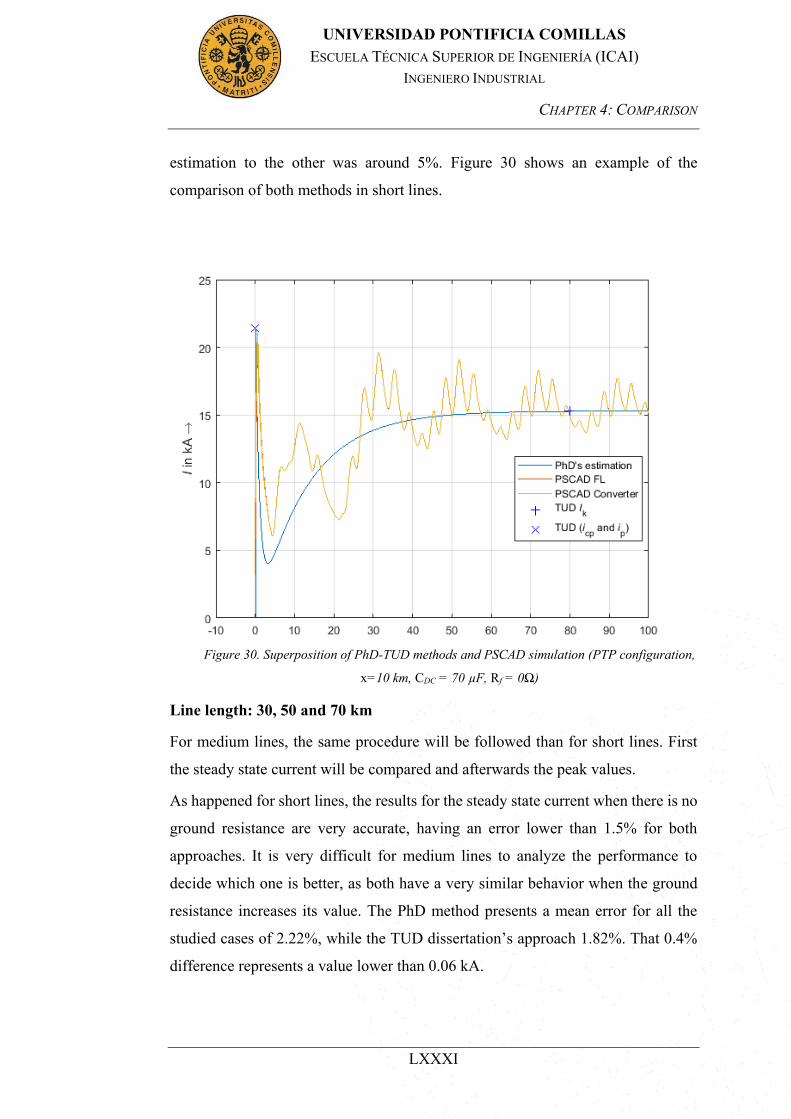
CHAPTER 4: COMPARISON
LXXXI
UNIVERSIDAD PONTIFICIA COMILLAS ESCUELA TÉCNICA SUPERIOR DE INGENIERÍA (ICAI)
INGENIERO INDUSTRIAL
estimation to the other was around 5%. Figure 30 shows an example of the
comparison of both methods in short lines.
Line length: 30, 50 and 70 km
For medium lines, the same procedure will be followed than for short lines. First
the steady state current will be compared and afterwards the peak values.
As happened for short lines, the results for the steady state current when there is no
ground resistance are very accurate, having an error lower than 1.5% for both
approaches. It is very difficult for medium lines to analyze the performance to
decide which one is better, as both have a very similar behavior when the ground
resistance increases its value. The PhD method presents a mean error for all the
studied cases of 2.22%, while the TUD dissertation’s approach 1.82%. That 0.4%
difference represents a value lower than 0.06 kA.
Figure 30. Superposition of PhD-TUD methods and PSCAD simulation (PTP configuration,
x=10 km, CDC = 70 µF, Rf = 0Ω)

CHAPTER 4: COMPARISON
LXXXII
UNIVERSIDAD PONTIFICIA COMILLAS ESCUELA TÉCNICA SUPERIOR DE INGENIERÍA (ICAI)
INGENIERO INDUSTRIAL
When the peak values are to be studied, a clear difference can be observed between
the estimations for the capacitor contribution’s peak and the total peak current,
being the capacitor contribution peak’s estimation significantly worse than the total
peak current’s estimation.
For the capacitor contribution’s peak the first situation to be studied is a variation
of the DC capacitor and a fixed value of ground resistance to 0 Ω. The mean error,
under these circumstances, for the PhD’s method is around 13-14%, while the TU
Darmstadt’s one is in the range of 10-11%. Knowing this data, it can be said that
the PhD’s methods performs slightly worse for these estimations. When the ground
resistance changes its value, it can be observed that the Darmstadt’s method works
better for low values of resistance, and when big values are studied, the PhD’s
approach is the one which works better.
On the other hand, the total peak current presents for both methods, errors below
7%, being in some situations below 0.5% for the TU Darmstadt’s approach. In this
case the results observed are constant and does not vary with DC capacitor’s nor
ground resistance’s changes. In every situation observed, the TU Darmstadt’s
method has a better performance.
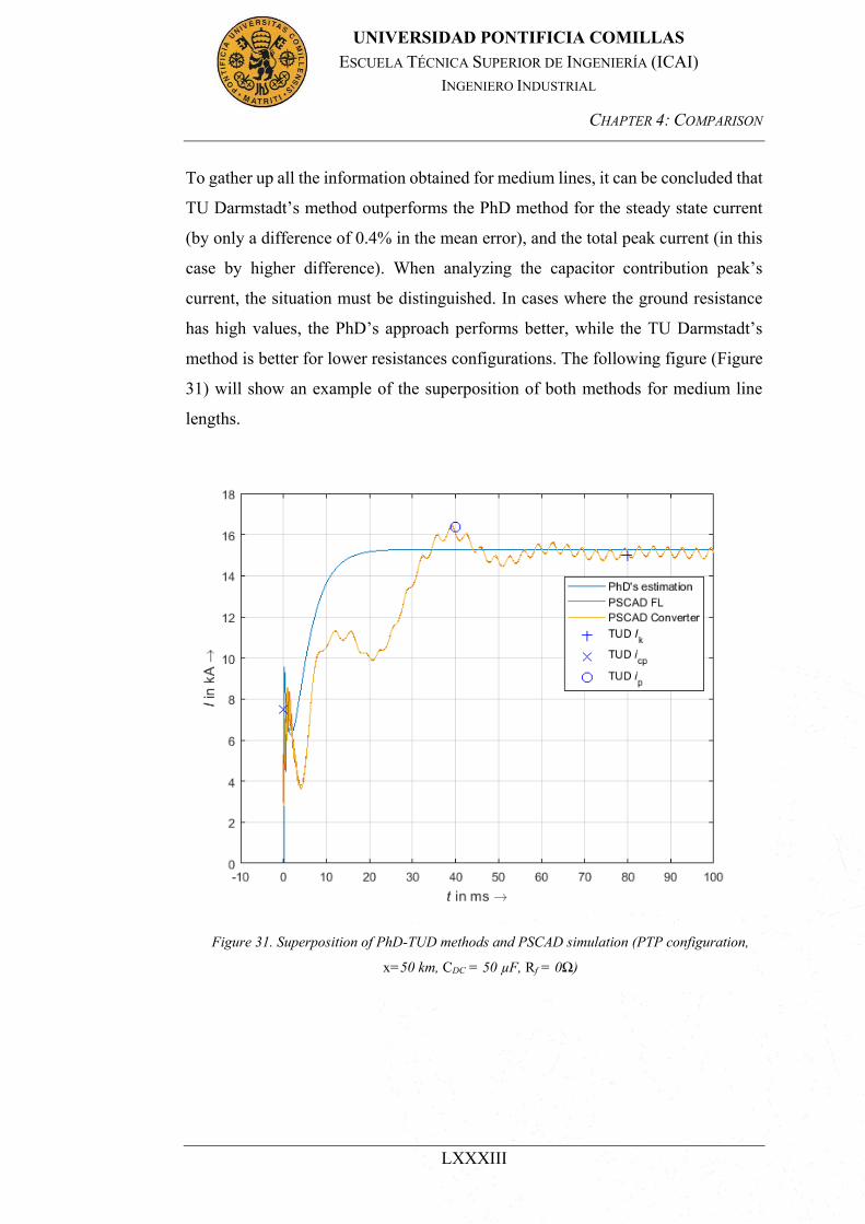
CHAPTER 4: COMPARISON
LXXXIII
UNIVERSIDAD PONTIFICIA COMILLAS ESCUELA TÉCNICA SUPERIOR DE INGENIERÍA (ICAI)
INGENIERO INDUSTRIAL
To gather up all the information obtained for medium lines, it can be concluded that
TU Darmstadt’s method outperforms the PhD method for the steady state current
(by only a difference of 0.4% in the mean error), and the total peak current (in this
case by higher difference). When analyzing the capacitor contribution peak’s
current, the situation must be distinguished. In cases where the ground resistance
has high values, the PhD’s approach performs better, while the TU Darmstadt’s
method is better for lower resistances configurations. The following figure (Figure
31) will show an example of the superposition of both methods for medium line
lengths.
Figure 31. Superposition of PhD-TUD methods and PSCAD simulation (PTP configuration,
x=50 km, CDC = 50 µF, Rf = 0Ω)
CHAPTER 4: COMPARISON
LXXXIV
UNIVERSIDAD PONTIFICIA COMILLAS ESCUELA TÉCNICA SUPERIOR DE INGENIERÍA (ICAI)
INGENIERO INDUSTRIAL
Line length: 100 km
The last case to be analyzed in the point to point configurations are the long lines.
For long lines, it is curious to observe how the TU Darmstadt’s method worsens its
performance. While the steady state current’s estimation has been proved to be
better for short and medium lines when the Darmstadt dissertation’s equations were
applied, in this case the PhD’s equations lead to better results. The difference
between the methods is more noticeable for low values of ground resistance, while
that difference shortens as the ground resistance increases. The reduction in that
error’s difference is not enough to change which approach is better and the PhD
outperforms the TUD’s method in every situation by 3% in the most extreme case
and 0.3% for higher values of ground resistance.
The capacitor contribution peak current’s estimation presents the highest difference
in long lines estimations. While the TU Darmstadt’s dissertation achieves error
below 10% in all cases, the PhD reaches error of almost 17%. This difference is
present for every parameter configuration (both for low and high DC capacitor and
ground resistance values).
On the other hand, when the total peak current is the value studied, almost no
difference can be observed in the estimations. Both methods have very good
estimations being the results in most cases below 3%. The only differences that can
be observed is that the PhD’s approach performs better in situations where the
ground resistance is at its maximum level (4 Ω) and the DC capacitor is also at its
maximum values (100 µF).
To sum up the analysis of long lines, it can be concluded that the PhD has better
estimations for the steady state current in every situation. On the other hand, the
dissertation’s results for both capacitor contribution’s peak and total peak current
are better (except the capacitor contribution’s peak for configurations with 4 Ω and
100 µF). The following figure (Figure 32) will show an example of the
superposition of both methods for long line lengths.

CHAPTER 4: COMPARISON
LXXXV
UNIVERSIDAD PONTIFICIA COMILLAS ESCUELA TÉCNICA SUPERIOR DE INGENIERÍA (ICAI)
INGENIERO INDUSTRIAL
MULTITERMINAL NETWORK
Once the PTP configurations have been studied, the approaches will be tested now
in multiterminal networks. These networks are characterized by the fact that the
transmission interaction occurs between three of more converters. In this case, the
topology which is used is the one already mentioned (
). This topology consists of four different converters in which the fault occurs in the
line that connects the node 1 and node 2. The distance at which this fault occurs
measured from node 1 will be changed. As it was done for PTP configuration, the
values of DC capacitor and ground resistance will also change in order to gather as
much data as possible and extract the best possible conclusions.
Three different groups will be done: short lines, medium lines and long lines. For
each of those groups a wide range of DC capacitor and ground resistance values
Figure 32. Superposition of PhD-TUD methods and PSCAD simulation (PTP
configuration, x=100 km, CDC = 50 µF, Rf = 0Ω)

CHAPTER 4: COMPARISON
LXXXVI
UNIVERSIDAD PONTIFICIA COMILLAS ESCUELA TÉCNICA SUPERIOR DE INGENIERÍA (ICAI)
INGENIERO INDUSTRIAL
will be varied and the steady state current, capacitor contribution peak and total
peak current values will be measured and compared to the PSCAD values.
Line length: 10 km
In this first case, the fault occurs at 10 km from the converter in node 1. In this
situation, the errors which are measured for the steady state current are under 3%
for every parameter combination and for both methods. This means that the
estimations done have great accuracy. By the sensibility analysis done in
“Comparison with PSCAD simulations” and “Comparison with PSCAD
simulations”, it can also be seen that changes in the DC capacitor and ground
resistance do not yield to big changes in the error. An explanation to this can be that
when a multiterminal network is studied, there are much more parameters that affect
the transient response of the system and changes in just one parameter are less
critical that those same changes for point to point configurations.
Even though both approaches obtain very good results, the PhD’s equations are
slightly better for steady state current’s estimations, having an error of only 0.24 %
for this configuration.
When the peak currents (both the capacitor’s contribution and the total peak) are
analyzed, it can be seen how PhD’s approach is very consistent, presenting very
little error difference against changes in DC capacitor and ground resistance. On
the other hand, the results from the TU Darmstadt’s dissertation present a higher
variability in the error for changes in the parameters.
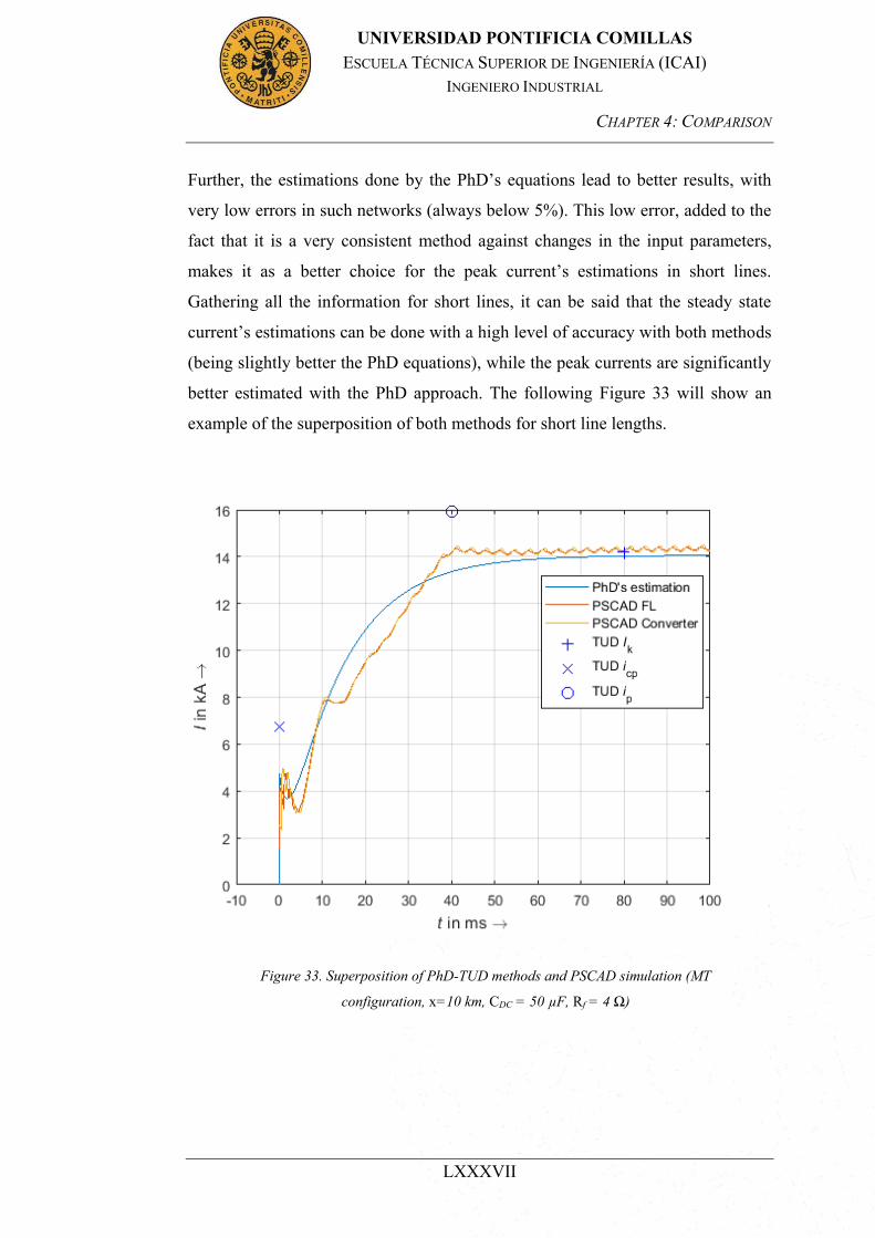
CHAPTER 4: COMPARISON
LXXXVII
UNIVERSIDAD PONTIFICIA COMILLAS ESCUELA TÉCNICA SUPERIOR DE INGENIERÍA (ICAI)
INGENIERO INDUSTRIAL
Further, the estimations done by the PhD’s equations lead to better results, with
very low errors in such networks (always below 5%). This low error, added to the
fact that it is a very consistent method against changes in the input parameters,
makes it as a better choice for the peak current’s estimations in short lines.
Gathering all the information for short lines, it can be said that the steady state
current’s estimations can be done with a high level of accuracy with both methods
(being slightly better the PhD equations), while the peak currents are significantly
better estimated with the PhD approach. The following Figure 33 will show an
example of the superposition of both methods for short line lengths.
Figure 33. Superposition of PhD-TUD methods and PSCAD simulation (MT
configuration, x=10 km, CDC = 50 µF, Rf = 4 Ω)
CHAPTER 4: COMPARISON
LXXXVIII
UNIVERSIDAD PONTIFICIA COMILLAS ESCUELA TÉCNICA SUPERIOR DE INGENIERÍA (ICAI)
INGENIERO INDUSTRIAL
Line lengths: 30, 50 and 70 km
In these cases, the fault occurs at a medium distance from the converter. Three
different cases are studied, which happen to behave the same way, so it makes the
sense the aggrupation of these three cases.
As happened for short lines, the accuracy of both methods for the steady state
current, regardless of the value of the DC capacitor and ground resistance is very
high. In both methods, the maximum error is not above 3.5 % and the differences
are very low. Nevertheless, the TU Darmstadt dissertation’s equations yield results
with errors below 0.25%.
On the other hand, TU Darmstadt’s method struggles with the peak values’
estimation. Specially with the capacitor current’s peak, where errors up to 25% can
be observed. In these cases, the PhD approach is more consistent and the errors do
not exceed 5%.
If the estimated value is the total peak’s current, the error for the TU Darmstadt’s
dissertation improves significantly to errors below 10%, but the PhD remains as a
better choice due to the fact that for the most unfavorable case, the error is 5%.
As a conclusion, it can be said that for medium distances the steady state current is
estimated with very low error by both methods, being slightly better with the TU
Darmstadt’s equations. When the peak values are the studied values, the PhD
approach is clearly better for that purpose, presenting itself as a very consistent
method, whose error is not altered by changes in the parameter’s configuration. The
following Figure 34 will show an example of the superposition of both methods for
medium line lengths.
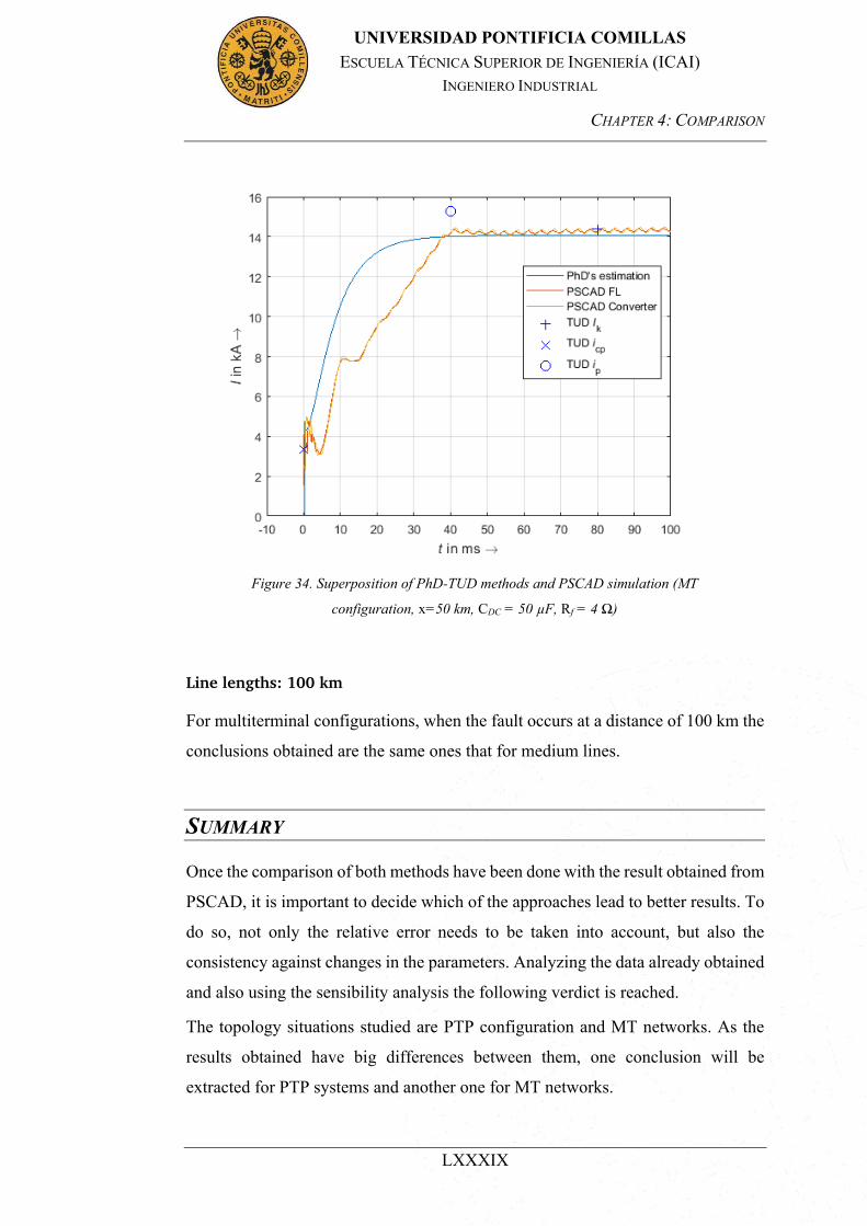
CHAPTER 4: COMPARISON
LXXXIX
UNIVERSIDAD PONTIFICIA COMILLAS ESCUELA TÉCNICA SUPERIOR DE INGENIERÍA (ICAI)
INGENIERO INDUSTRIAL
Line lengths: 100 km
For multiterminal configurations, when the fault occurs at a distance of 100 km the
conclusions obtained are the same ones that for medium lines.
SUMMARY
Once the comparison of both methods have been done with the result obtained from
PSCAD, it is important to decide which of the approaches lead to better results. To
do so, not only the relative error needs to be taken into account, but also the
consistency against changes in the parameters. Analyzing the data already obtained
and also using the sensibility analysis the following verdict is reached.
The topology situations studied are PTP configuration and MT networks. As the
results obtained have big differences between them, one conclusion will be
extracted for PTP systems and another one for MT networks.
Figure 34. Superposition of PhD-TUD methods and PSCAD simulation (MT
configuration, x=50 km, CDC = 50 µF, Rf = 4 Ω)

CHAPTER 4: COMPARISON
XC
UNIVERSIDAD PONTIFICIA COMILLAS ESCUELA TÉCNICA SUPERIOR DE INGENIERÍA (ICAI)
INGENIERO INDUSTRIAL
The results obtained for PTP situations are very accurate with the two different
approaches. Checking the results obtained for the steady state current, it can be
affirmed that for short and medium lines, Darmstadt’s equations have better results,
while for long lines, the equations proposed in the PhD are minimally more
accurate. In every case, the errors that were obtained are below 5%. This error
comes from neglecting the influence that the harmonics have on the steady state
current. The equations developed only take into account the sixth harmonic and the
rest of them, which do have influence on the steady state value.
For the peak values, also good results were obtained from the simulations. In this
case, the PhD equations reach more precise estimations for short lines, while for
medium and long lines the Darmstadt method presents itself as more consistent.
With the correct analysis of this information and knowing that some metrics are
more beneficial to one or the other method it can be concluded that when the whole
range of analysis is studied, the TUD Dissertation presents itself as a more reliable
approach for PTP networks. In the total comparison, there are more situations in
which this method has better results.
One clarification that must be done is related to the capacitor contribution’s peak.
As it was already discussed in 0, the PhD method applies a correction factor to this
peak value. Even though, in the majority of the situations studied, this factor
improves the performance when it is set to 0.88, there might be situations (different
parameters, converters, etc.) in which the results do not perform the same manner.
The second configuration tested was the multiterminal network. These kind of
networks are characterized by the presence of more than two converters. In the
studied case, a four node system was chosen.
In this case, changes in the distance to the fault does not affect so much the final
results and for the three lines studied (short, medium and long lines), the same
conclusion can be extracted. For MT networks, the results lead to bigger differences
in the current estimations. The results of the PhD method are better for every
analyzed situation. Also, the changes that the estimations suffer against variations
in the parameters are smaller than in the TUD Dissertation’s method. These

CHAPTER 4: COMPARISON
XCI
UNIVERSIDAD PONTIFICIA COMILLAS ESCUELA TÉCNICA SUPERIOR DE INGENIERÍA (ICAI)
INGENIERO INDUSTRIAL
differences are more noticeable in the peak current’s estimations, while for the
steady state current, the difference is significantly smaller.
For all the exposed reasons and results, it can be said that for PTP configurations,
the TU Darmstadt approach is more accurate, while when MT networks are studied,
the PhD method is the best choice for the current estimations.

CHAPTER 5: CONCLUSIONS
XCII
UNIVERSIDAD PONTIFICIA COMILLAS ESCUELA TÉCNICA SUPERIOR DE INGENIERÍA (ICAI)
INGENIERO INDUSTRIAL
CHAPTER 5 : CONCLUSIONS
Once all the simulations and comparisons have been done, interesting conclusions
can be extracted from the work done. Two main configurations have been studied,
which are point-to-point configurations and multiterminal network. In both of these
configurations, changes in the parameter’s definition have been applied in order to
have a wider range of data to analyse. The parameters which have been varied are
the value of the DC capacitor, the ground resistance and the distance from the
converter to the fault.
The main objective of the thesis is to compare the accuracy that the two proposed
methods have under different situations. To do so, first a sensibility analysis was
done to determine which are the optimal conditions for the different methods. The
outcome of that analysis was the following one:
For point to point configurations the first method (PhD) presents differences in the
results for short, medium and long lines. Nevertheless, in general, the steady state
current’s estimation is better when low values of ground resistances are defined,
while it does not present any changes against variations of the DC capacitor.
Moreover, the peak values of the current have better results under low DC
capacitors.
The second method (TUD) also presents differences between parameters changes
for short, medium and long lines. General results conclude that the DC capacitor
does not affect the results of the steady state current. This current is only affected
by changes in the ground resistance, and presents better estimations for low values.
On the other hand, the peak currents do not present a clear tendency against changes
in the DC capacitor, whereas an increase in the ground resistance increases the error
in the peak estimations.
The conclusions obtained for the point to point configurations can be extrapolated
to the multiterminal networks with some differences. One of the most important
differences is that changes in the DC capacitor and ground resistance, as well as the
CHAPTER 5: CONCLUSIONS
XCIII
UNIVERSIDAD PONTIFICIA COMILLAS ESCUELA TÉCNICA SUPERIOR DE INGENIERÍA (ICAI)
INGENIERO INDUSTRIAL
fault distance have less influence in multiterminal networks, as there are more
parameters which affect the transient behaviour of the system.
This analysis is very important to see which situations or parameters affect more to
the proposed methods and is very helpful in order to decide which approach
presents better and more reliable results.
With the objective to reach a verdict on determining which approach is better for
the purpose, all the information must be gathered up. Not only one result can be
used in order to determine a final decision. The sensibility analysis and the
comparison chapters were key analysis to reach a conclusion. As it was said before,
the results obtained are different for PTP configurations and MT networks, so
different conclusions will be exposed for each case.
By using the whole range of parameters combinations and analysing the different
configurations, it can be said that two main aspects determine which method is more
suitable. The first condition is the relative error that the estimations have for the
three characteristic points of the transient current (steady state, total peak, capacitor
contribution’s peak). The second aspect that must be taken into account is the
robustness that the results have for different situations. It is desired a method that
do not experiment big changes in the error when the parameters change.
Taking these features into account, it can be said that PTP configurations are more
suitable for TU Darmstadt’s dissertation method, while MT networks are better for
the performance of the PhD’s approach.
CHAPTER 6: OUTLOOK
XCV
UNIVERSIDAD PONTIFICIA COMILLAS ESCUELA TÉCNICA SUPERIOR DE INGENIERÍA (ICAI)
INGENIERO INDUSTRIAL
CHAPTER 6 : OUTLOOK
Once the analysis in order to determine how much difference exists between the
two proposed methods in the exposed situations is done, there are some areas which
seem to be unsolved. These areas can be applicable both for point to point
configurations and multiterminal networks or it can be specific only to one of them.
One of the aspects that can be changed are the characteristics of the converter. Even
though, the PhD method is only applicable to two-level converters, the
characteristics that define these converters can be changed and studied.
These changes in the converter can be done both for PTP and MT networks. It is
interesting to check if the obtained results are equivalent for different voltage levels
or armature inductances.
Another feature to have in mind is the type of line and the internal resistance of
them. In the original publications, it is exposed that the proposed equations are valid
also for overhead lines, but in none of the publications an extent analysis have been
done.
Being more specific into MT networks, in the actual thesis only one topology has
been studied. This decision was taken due to the fact the proposed equations for
equivalent resistances and inductances were only valid for the given configuration.
An interesting improvement in this topic would be to propose formulas for these
equivalent resistances and inductances regardless the number of nodes and the
connections between them.
Another aspect, related also with the equivalent resistances for MT networks is the
location of the fault. In the studied cases, the fault always occurs at the same place.
By changing the location of the fault (in other nodes), the transient current may be
more or less affected.

REFERENCES
XCVI
UNIVERSIDAD PONTIFICIA COMILLAS ESCUELA TÉCNICA SUPERIOR DE INGENIERÍA (ICAI)
INGENIERO INDUSTRIAL
REFERENCES
XCVII
UNIVERSIDAD PONTIFICIA COMILLAS ESCUELA TÉCNICA SUPERIOR DE INGENIERÍA (ICAI)
INGENIERO INDUSTRIAL
REFERENCES
[1] M. Eghlimi and S. G. Hamed, “Economic analysis of Iran-Turkey power network interconnection: HVDC vs. HVAC,” PECon 2008 - 2008 IEEE 2nd Int. Power Energy Conf., no. PECon 08, pp. 164–168, 2008.
[2] M. P. Bahrman and B. K. Johnson, “The ABCs of HVDC transmission technologies,” IEEE Power Energy Mag., 2007.
[3] A. Wasserrab and G. Balzer, “Determination of DC Short-Circuit Currents of MMC-HVDC Converters for DC Circuit Breaker Dimensioning.”
[4] X. Feng, L. Qi, and Z. Wang, “Estimation of short circuit currents in mesh DC networks,” in IEEE Power and Energy Society General Meeting, 2014.
[5] A. Wasserrab and G. Balzer, “Calculation of Short Circuit Currents in HVDC Systems.”
[6] A. Wasserrab, B. Just, and G. Balzer, “Contribution of HVDC converters to the DC short circuit current,” in Proceedings of the Universities Power Engineering Conference, 2013.
[7] J. Brown, J. Allan, and M. B. Mellitt, “Six-pulse three-phase rectifier bridge models for calculating closeup and remote short circuit transients on DC supplied railways.”
[8] V. Akhmatov et al., “Technical guidelines and prestandardization work for first HVDC Grids,” IEEE Trans. Power Deliv., 2014.
[9] P. Pozzobon, “Transient and steady-state short-circuit currents in rectifiers for DC traction supply,” IEEE Trans. Veh. Technol., 1998.
[10] S. Skok, A. Marusic, and S. Tesnjak, “Transient short - Circuit currents in auxiliary DC installations in power plants and substations,” in 2003 IEEE Bologna PowerTech - Conference Proceedings, 2003.
[11] M. K. Bucher, “Transient Fault Currents in HVDC VSC Networks During Pole-to- Ground Faults ETH Library,” 2014.
[12] M. K. Bucher and C. M. Franck, “Analytic Approximation of Fault Current Contribution from AC Networks to MTDC Networks during Pole-to-Ground Faults,” IEEE Trans. Power Deliv., 2016.
[13] M. K. Bucher and C. M. Franck, “Analytic approximation of fault current contributions from capacitive components in HVDC cable networks,” IEEE Trans. Power Deliv., 2015.
[14] Dipl-Ing Andreas Wasserrab, D.-I. Gerd Balzer Korreferent, rer M. nat Christian Franck Korreferent, and D.-I. Jutta Hanson, “Kurzschlussstromberechnung in Gleichstromnetzen der elektrischen Leistungsübertragung,” 2016.

REFERENCES
XCVIII
UNIVERSIDAD PONTIFICIA COMILLAS ESCUELA TÉCNICA SUPERIOR DE INGENIERÍA (ICAI)
INGENIERO INDUSTRIAL
[15] W. Wang et al., “Cascaded H7 Current Source Converter Based Power Transmission System and Fault Analysis,” pp. 0–6, 2006.
[16] M. Alhasheem, T. Dragicevic, M. Rivera, and F. Blaabjerg, “Losses Evaluation for a Two-Level Three-Phase Stand-Alone Voltage Source Converter Using Model Predictive Control.”
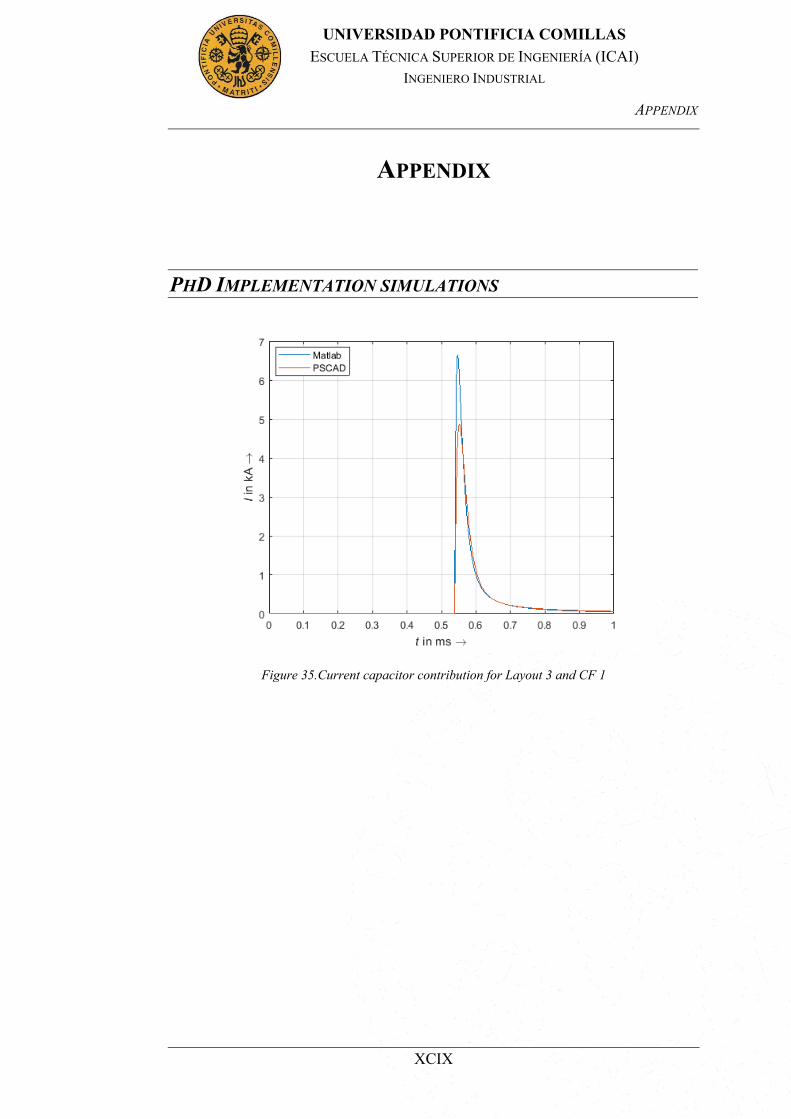
APPENDIX
XCIX
UNIVERSIDAD PONTIFICIA COMILLAS ESCUELA TÉCNICA SUPERIOR DE INGENIERÍA (ICAI)
INGENIERO INDUSTRIAL
APPENDIX
PHD IMPLEMENTATION SIMULATIONS
Figure 35.Current capacitor contribution for Layout 3 and CF 1

APPENDIX
C
UNIVERSIDAD PONTIFICIA COMILLAS ESCUELA TÉCNICA SUPERIOR DE INGENIERÍA (ICAI)
INGENIERO INDUSTRIAL
Figure 36. Current capacitor contribution for Layout 3 and CF 0.75
Figure 37. Current adjacent feeder contribution for Layout 3 and CF 1

APPENDIX
CI
UNIVERSIDAD PONTIFICIA COMILLAS ESCUELA TÉCNICA SUPERIOR DE INGENIERÍA (ICAI)
INGENIERO INDUSTRIAL
Figure 38. Current adjacent feeder contribution for Layout 3 and CF 0.75
Figure 39. CB Current for Layout 3 and CF 1

APPENDIX
CII
UNIVERSIDAD PONTIFICIA COMILLAS ESCUELA TÉCNICA SUPERIOR DE INGENIERÍA (ICAI)
INGENIERO INDUSTRIAL
Figure 40. CB Current for Layout 3 and CF 0.75
Figure 41. CB Current for Layout 1and CF 0.88
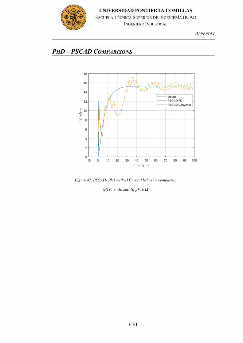
APPENDIX
CIII
UNIVERSIDAD PONTIFICIA COMILLAS ESCUELA TÉCNICA SUPERIOR DE INGENIERÍA (ICAI)
INGENIERO INDUSTRIAL
PHD – PSCAD COMPARISONS
Figure 42. PSCAD- Phd method Current behavior comparison
(PTP, x=30 km, 10 µF, 0 Ω)
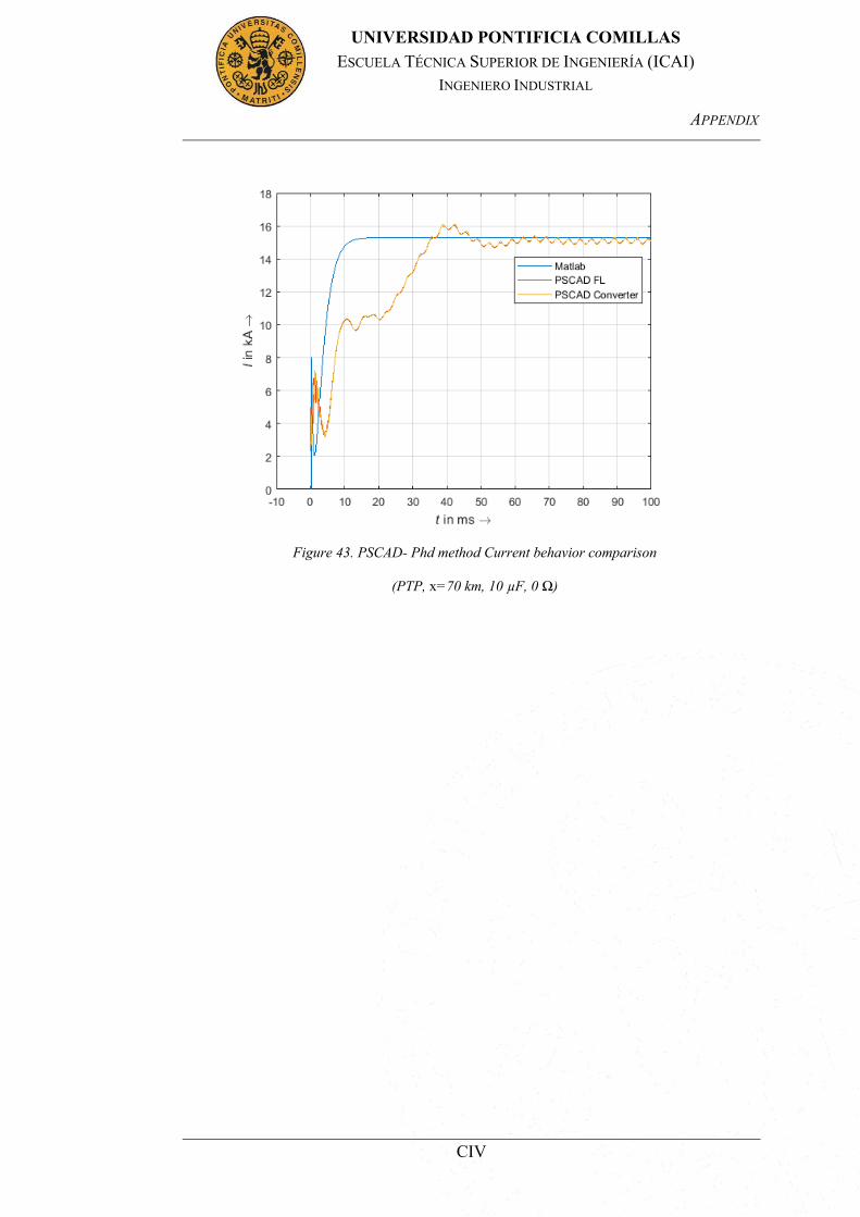
APPENDIX
CIV
UNIVERSIDAD PONTIFICIA COMILLAS ESCUELA TÉCNICA SUPERIOR DE INGENIERÍA (ICAI)
INGENIERO INDUSTRIAL
Figure 43. PSCAD- Phd method Current behavior comparison
(PTP, x=70 km, 10 µF, 0 Ω)
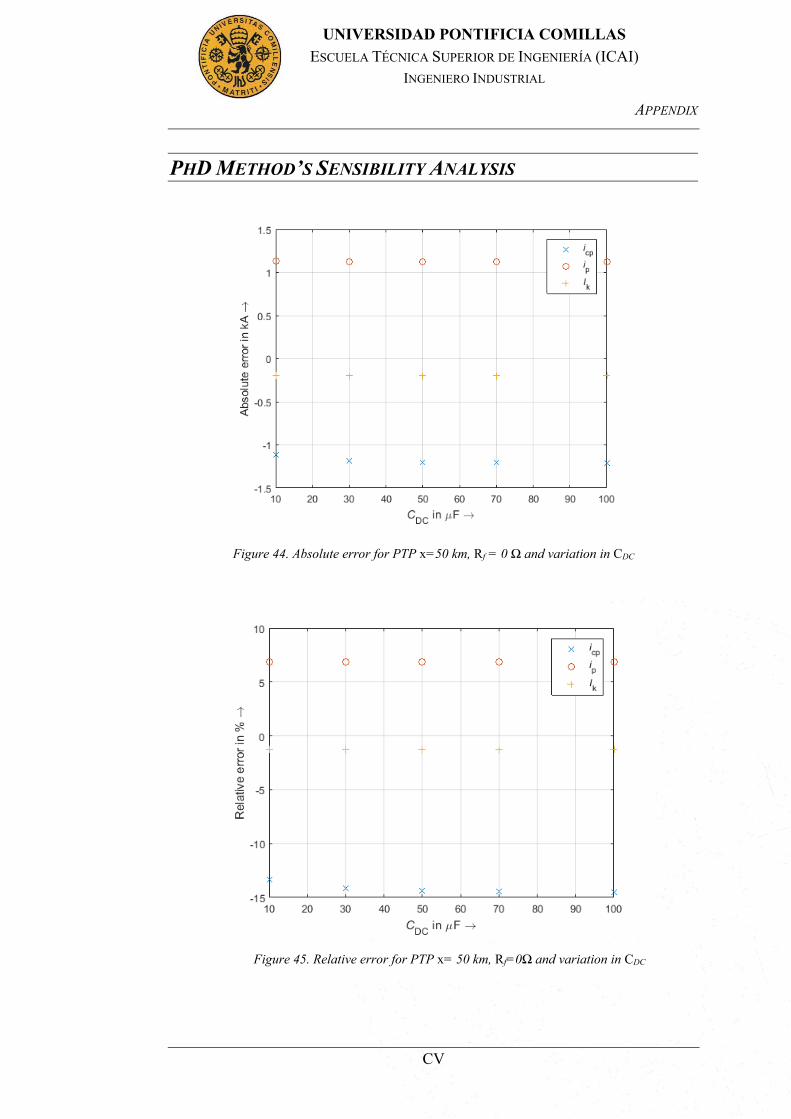
APPENDIX
CV
UNIVERSIDAD PONTIFICIA COMILLAS ESCUELA TÉCNICA SUPERIOR DE INGENIERÍA (ICAI)
INGENIERO INDUSTRIAL
PHD METHOD’S SENSIBILITY ANALYSIS
Figure 45. Relative error for PTP x= 50 km, Rf=0Ω and variation in CDC
Figure 44. Absolute error for PTP x=50 km, Rf = 0 Ω and variation in CDC
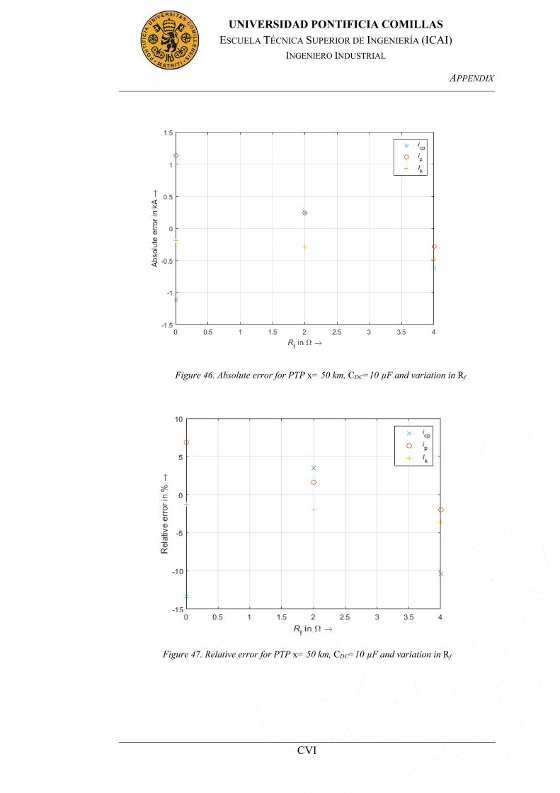
APPENDIX
CVI
UNIVERSIDAD PONTIFICIA COMILLAS ESCUELA TÉCNICA SUPERIOR DE INGENIERÍA (ICAI)
INGENIERO INDUSTRIAL
Figure 46. Absolute error for PTP x= 50 km, CDC=10 µF and variation in Rf
Figure 47. Relative error for PTP x= 50 km, CDC=10 µF and variation in Rf

APPENDIX
CVII
UNIVERSIDAD PONTIFICIA COMILLAS ESCUELA TÉCNICA SUPERIOR DE INGENIERÍA (ICAI)
INGENIERO INDUSTRIAL
Figure 48. Absolute error for PTP configuration and different distances
Figure 49. Relative error for PTP configuration and different distances

APPENDIX
CVIII
UNIVERSIDAD PONTIFICIA COMILLAS ESCUELA TÉCNICA SUPERIOR DE INGENIERÍA (ICAI)
INGENIERO INDUSTRIAL
Figure 50. Absolute error for MT x = 10 km, CDC = 10 µF and variation in Rf
Figure 51. Relative error for MT x = 10 km, CDC = 10 µF and variation in Rf

APPENDIX
CIX
UNIVERSIDAD PONTIFICIA COMILLAS ESCUELA TÉCNICA SUPERIOR DE INGENIERÍA (ICAI)
INGENIERO INDUSTRIAL
Figure 52. Absolute error for MT x = 50 km, CDC = 10 µF and variation in Rf
Figure 53. Relative error for MT x = 50 km, CDC = 10 µF and variation in Rf

APPENDIX
CX
UNIVERSIDAD PONTIFICIA COMILLAS ESCUELA TÉCNICA SUPERIOR DE INGENIERÍA (ICAI)
INGENIERO INDUSTRIAL
Figure 54. Absolute error for MT configuration and different distances
Figure 55. Relative error for MT configuration and different distances

APPENDIX
CXI
UNIVERSIDAD PONTIFICIA COMILLAS ESCUELA TÉCNICA SUPERIOR DE INGENIERÍA (ICAI)
INGENIERO INDUSTRIAL
TUD METHOD’S SENSIBILITY ANALYSIS
Figure 56. Absolute error for PTP x = 50 km, Rf = 0 Ωand variation in CDC
Figure 57. Relative error for PTP x = 50 km, Rf = 0 Ωand variation in CDC

APPENDIX
CXII
UNIVERSIDAD PONTIFICIA COMILLAS ESCUELA TÉCNICA SUPERIOR DE INGENIERÍA (ICAI)
INGENIERO INDUSTRIAL
Figure 58. Absolute error for PTP x = 50 km, CDC = 10 µF and variation in Rf
Figure 59. Relative error for PTP x = 50 km, CDC = 10 µF and variation in Rf
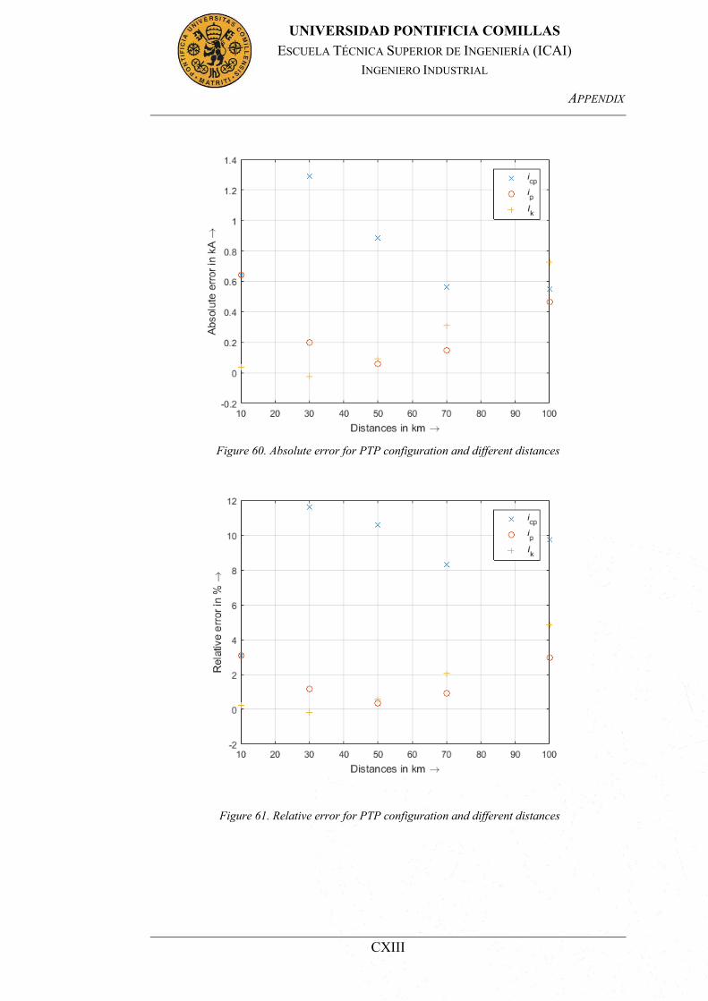
APPENDIX
CXIII
UNIVERSIDAD PONTIFICIA COMILLAS ESCUELA TÉCNICA SUPERIOR DE INGENIERÍA (ICAI)
INGENIERO INDUSTRIAL
Figure 60. Absolute error for PTP configuration and different distances
Figure 61. Relative error for PTP configuration and different distances

APPENDIX
CXIV
UNIVERSIDAD PONTIFICIA COMILLAS ESCUELA TÉCNICA SUPERIOR DE INGENIERÍA (ICAI)
INGENIERO INDUSTRIAL
Figure 62. Absolute error for MT x = 10 km, Rf = 2 Ωand variation in CDC
Figure 63. Relative error for MT x = 10 km, Rf = 2 Ω and variation in CDC

APPENDIX
CXV
UNIVERSIDAD PONTIFICIA COMILLAS ESCUELA TÉCNICA SUPERIOR DE INGENIERÍA (ICAI)
INGENIERO INDUSTRIAL
Figure 64. Absolute error for MT x = 50 km, Rf = 2 Ω and variation in CDC
Figure 65. Relative error for MT x = 50 km, Rf = 2 Ωand variation in CDC
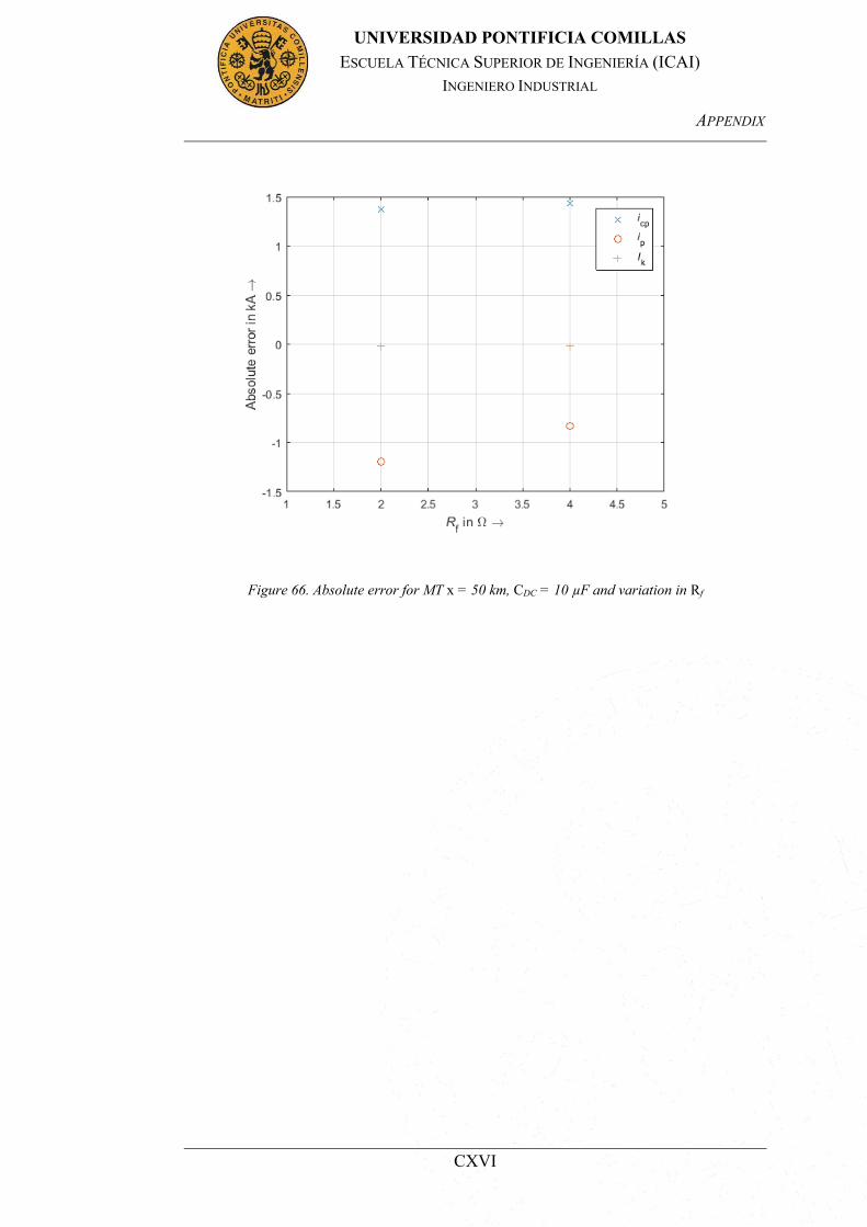
APPENDIX
CXVI
UNIVERSIDAD PONTIFICIA COMILLAS ESCUELA TÉCNICA SUPERIOR DE INGENIERÍA (ICAI)
INGENIERO INDUSTRIAL
Figure 66. Absolute error for MT x = 50 km, CDC = 10 µF and variation in Rf

APPENDIX
CXVII
UNIVERSIDAD PONTIFICIA COMILLAS ESCUELA TÉCNICA SUPERIOR DE INGENIERÍA (ICAI)
INGENIERO INDUSTRIAL
Figure 67. Relative error for MT x = 50 km, CDC = 10 µF and variation in Rf
Figure 68. Absolute error for MT configuration and different distances
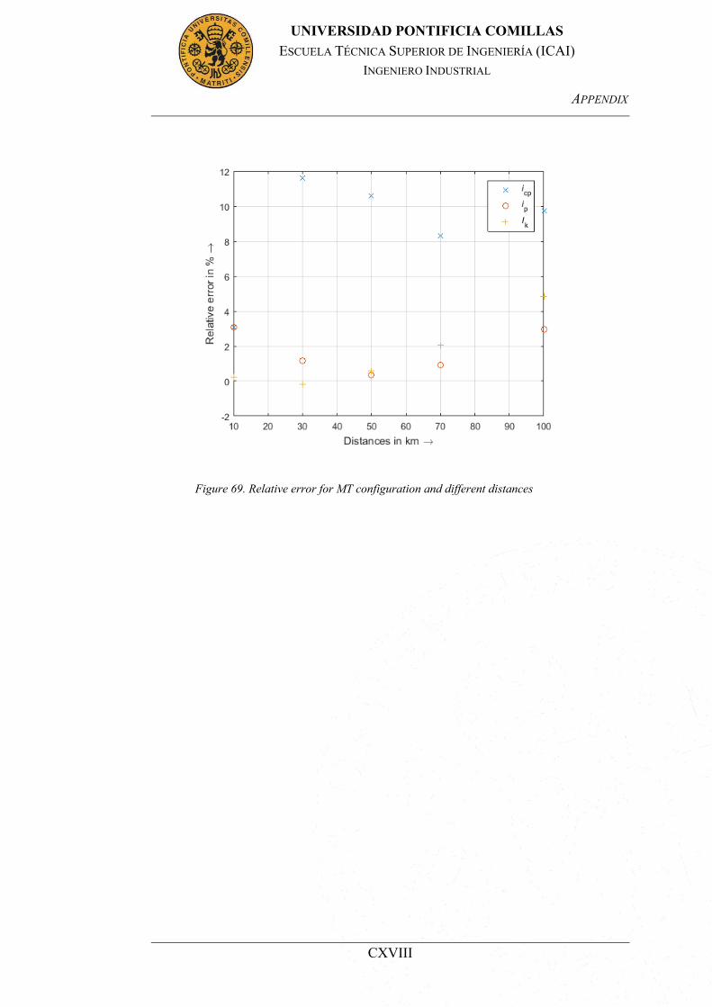
APPENDIX
CXVIII
UNIVERSIDAD PONTIFICIA COMILLAS ESCUELA TÉCNICA SUPERIOR DE INGENIERÍA (ICAI)
INGENIERO INDUSTRIAL
Figure 69. Relative error for MT configuration and different distances