CENTRO DE INVESTIGACIÓN EN MATERIALES

AVANZADOS S.C.

DEPARTAMENTO DE ESTUDIOS DE POSGRADO

Graduate School

Synthesis and characterization of sodium silicate obtained by

different chemical routes (Síntesis y caracterización de silicato de sodio obtenido por diferentes rutas químicas)

THESIS SUBMITTED IN PARTIAL FULLMILMENT OF THE

REQUIREMEMENTS FOR THE DEGREE OF

MASTER IN MATERIALS SCIENCE

PRESENTED BY:

Eng. Armando Tejeda Ochoa

ADVISOR:

José Martín Herrera Ramírez, Ph.D.

CHIHUAHUA, CHIH. November, 2015

ABSTRACT

Silicon is the second most abundant element in Earth’s crust (28% compared to oxygen at 46%)

occurring as silicon dioxide (sand, flint, quartz) and various silicates.

Sodium silicate is the generic name given to a series of compounds derived from soluble sodium

silicate glass. Aqueous solutions are important in biology, geology and numerous technical

processes including for example the manufacturing of sol gels and zeolites. Sodium silicate is also

used as an activator for geopolymer cements synthesis, which are a low carbon emission type.

When silicates are combined with cement ingredients, they react chemically in order to form

masses with strong binding properties.

In this study different silica sands have been investigated in order to synthesize sodium silicate,

which has several applications in the industry. All the silica sand banks were compared with a

control sample, then different reactions were studied and performed in order to obtain the best

sodium silicate. All reactions were evaluated and their products characterized, which comprised

structural and microstructural analysis including, but not limited to, thermogravimetric analysis,

scanning electron microscopy, energy dispersive spectrometry, Fourier transform infrared

spectroscopy (FTIR), Raman spectroscopy, X-ray fluorescence (XRF) and X-ray powder

diffraction (XRD). The best reaction is presented and discussed.

RESUMEN

El silicio es el segundo elemento más abundante en la corteza terrestre (28% comparado con el

oxígeno 46%) y se presenta como dióxido de silicio (arena, piedra, cuarzo) y varios silicatos.

Silicato de sodio es el nombre genérico dado a una serie de compuestos derivados del silicato de

sodio soluble. Soluciones acuosas de silicato son importantes en biología, geología y un número

de procesos químicos incluyendo por ejemplo la manufactura de sol geles y zeolitas. El silicato de

sodio es también usado como activador para la síntesis de cementos geopoliméricos, los cuales son

reconocidos por presentar una baja huella de carbono. Cuando los silicatos son combinados con

ingredientes del cemento, reaccionan químicamente para formar masas con fuertes propiedades

ligantes.

En este estudio, diferentes arenas fueron investigadas con la finalidad de sintetizar silicato de

sodio, el cual tiene diversas aplicaciones de interés en la industria. Todos los bancos de arenas

fueron comparados con una muestra testigo, diferentes reacciones fueron estudiadas y llevadas a

cabo con el fin de obtener el mejor silicato de sodio. Todas las reacciones fueron evaluadas y sus

productos caracterizados, lo cual comprendió el análisis estructural y microestructural incluyendo,

pero no limitados a, análisis termogravimétrico, microscopía electrónica de barrido, análisis

elemental, espectroscopía de infrarroja por transformada de Fourier (FTIR), espectroscopía

Raman, fluorescencia de rayos-X (XRF ) y difracción de rayos-X (XRD). Se presenta y discute la

mejor reacción

TABLE OF CONTENTS

TABLE OF CONTENTS ............................................................................................. v

TABLE OF FIGURES ................................................................................................. viii

TABLE OF INDEX ..................................................................................................... xi

AKNOWLEDGMENTS .............................................................................................. xii

JUSTIFICATION ........................................................................................................ 14

Chapter 1: Background ................................................................................................ 15

Silicon and their nature. ........................................................................................ 15 Applications of Silicon-based products. ........................................................ 16

Sodium silicate. ..................................................................................................... 16 Production of sodium silicate. ....................................................................... 17

Reactions: ............................................................................................... 19 Sodium silicate applications. ......................................................................... 19

Lower carbon footprint cements............................................................. 19

Hypothesis and Objectives ........................................................................................... 20

Hypothesis. ........................................................................................................... 20

General objective. ................................................................................................. 20

Specific objectives. ........................................................................................ 20

Chapter 2: Experimental methodology ........................................................................ 21

Fluorescence and X-ray diffractions. .................................................................... 21

X-ray diffraction. ........................................................................................... 22

Operation. ............................................................................................... 23 Sample preparation and equipment specifications. ................................ 25

X-ray fluorescence. ........................................................................................ 26 Operation. ............................................................................................... 26 Sample preparation and equipment specifications. ................................ 28

Optical microscope. .............................................................................................. 29

Components. .................................................................................................. 29

Lenses. ........................................................................................................... 30 Illumination. .................................................................................................. 30 Equipment specifications. .............................................................................. 31

Scanning electron microscopy. ............................................................................. 32 System components. ...................................................................................... 32

Electron gun. .......................................................................................... 33 Lenses. .................................................................................................... 34 Sample chamber. .................................................................................... 34

Detectors. ................................................................................................ 34

Vacuum chamber. ................................................................................... 35 Electron-sample interactions. ........................................................................ 35 Operation. ...................................................................................................... 36

Sample preparation and equipment specifications. ....................................... 37 Thermal analysis. .................................................................................................. 38

Differential thermal analysis (DTA). ............................................................ 38 Differential scanning calorimetry (DSC). ..................................................... 40

The heat flux DSC. ................................................................................. 40

Disk-type DSC…………………………………………………….................41

Cylinder-type DSC………………………………………………………...….41

Power compensating differential scanning calorimeters. ....................... 42 Thermogravimetric analysis (TGA). ............................................................. 43

TGA Design and experimental concerns. .............................................. 43 Equipment specifications. .............................................................................. 45

Thermocouples. .................................................................................................... 46 Common thermocouple types. ....................................................................... 46

T-type thermocouple. ............................................................................. 47 J-type thermocouple. .............................................................................. 47 K-type thermocouple. ............................................................................. 47

Sample preparation and equipment specifications. ....................................... 48 Fourier transform infra-red spectroscopy. ............................................................ 49

Operation. ...................................................................................................... 50

Equipment specifications. .............................................................................. 51

Raman spectroscopy. ............................................................................................ 51 Basic theory. .................................................................................................. 51

Origin of the Raman spectra. ......................................................................... 52 Raman active modes. ..................................................................................... 53 Raman equipment design. ............................................................................. 53

Excitation source. ................................................................................... 54 Sample holder. ........................................................................................ 54 Grating. ................................................................................................... 54

Filters. ..................................................................................................... 54 Detection system. ................................................................................... 54

Operation. ...................................................................................................... 55 Equipment specifications. .............................................................................. 55

Samples. ................................................................................................................ 57 Crushing and pulverization. .................................................................................. 58 Milling. ................................................................................................................. 58

Reaction procedure. .............................................................................................. 60 Experimental reaction. ................................................................................... 61

Chapter 3: Results and discussion................................................................................ 62

ΔG simulation. ...................................................................................................... 62

SILICA SAND BANKS ....................................................................................... 63 Optical microscopy. ....................................................................................... 63 Particle size distribution. ............................................................................... 65

Milling. ................................................................................................... 66 X-ray diffraction. ........................................................................................... 67 X-ray fluorescence. ........................................................................................ 69 Scanning electron microscopy. ...................................................................... 70 Thermogravimetric analysis. ......................................................................... 72

Fourier transform infra-red spectroscopy. ..................................................... 73 SODIUM SILICATE. ........................................................................................... 75

Thermal analysis. ........................................................................................... 75 X-ray diffraction. ........................................................................................... 78

Fourier transform infra-red spectroscopy. ..................................................... 80 Raman spectroscopy ...................................................................................... 82

Scanning electron microscopy. ...................................................................... 82

Chapter 4: Conclusions and future work ..................................................................... 85

Conclusions........................................................................................................... 85 Future work. .......................................................................................................... 87

References .................................................................................................................... 88

TABLE OF FIGURES

Figure 1: (a) Bragg's law for the case of a rectangular grid, i.e. AB = BC = d(hkl) sin θ: the

path difference (AB + BC) = 2d(hkl) sin θ. (b) Bragg's law for the general case in which

AB ≠ BC. Again, the path difference (AB + BC) = 2d(hkl) sin θ [22]. .................. 23

Figure 2: Arrangement of slits in a diffractometer [21]. .............................................. 23

Figure 3: Illustration of the process of inner-shell ionization and the subsequent emission

of a characteristic X-ray: (a) an incident electron ejects a K shell electron from an

atom, (b) leaving a hole in the K shell; (c) electron rearrangement occurs, resulting in

the emission of an X-ray photon [21]. .................................................................. 24

Figure 4: Bruker D8 advance diffractometer. .............................................................. 25

Figure 5: Fluorescent X-ray spectroscopy [18]. .......................................................... 28

Figure 6: Microscope optical components [23]. .......................................................... 31

Figure 7: Axio Scope A1 microscope. ......................................................................... 31

Figure 8: The two major parts of the SEM, the electron column and the electronics console

[24]. ....................................................................................................................... 33

Figure 9: Types of interactions between electrons and sample [25]. ........................... 36

Figure 10: Scanning electron microscopes. (a) JEOL 5800LV, (b) Hitachi SU3500.. 37

Figure 11: DTA measuring system with free standing crucibles. The crucibles are contacted

by thermocouples to measure ΔTSR and the reference temperature TR [31].......... 39

Figure 12: DTA block measuring system. The temperature sensors are located inside the

specimens [31]. ..................................................................................................... 39

Figure 13: Disc-type DSC [31]. ................................................................................... 41

Figure 14: Cylinder-type DSC [31]. ............................................................................ 42

Figure 15: Power compensating DSC [31]. ................................................................. 43

Figure 16: Example of a TGA design. As the specimen changes weight, its tendency to rise

or fall is detected by the LVDT. A current through the coil on the counterbalance side

exerts a force on the magnetic core which acts to return the balance pan to a null

position. The current required to maintain this position is considered proportional to

the mass change of the specimen [30]. ................................................................. 44

Figure 17: Gahn microbalance design [30]. ................................................................. 45

Figure 18: DSC Autosampler, TA instruments............................................................ 45

Figure 19: High temperature furnaces: (a) GSL1300X tube furnace, (b) Electra furnace.48

Figure 20: Michelson Interferometer [36]. .................................................................. 49

Figure 21: FTIR System Spectrum GX. ...................................................................... 51

Figure 22: Types of Raman scattering signals. ............................................................ 52

Figure 23: Horiba Xplora Raman spectrometer. .......................................................... 55

Figure 24: Aspect of a Lajas sand (a) before and (b) after the particle size reduction. 58

Figure 25: Equipment used to reduce and measure particle size. (a) High energy mixer mill,

(b) CILAS equipment. .......................................................................................... 59

Figure 26: ΔG simulation results of the different reactions. ........................................ 62

Figure 27: Control sample micrograph. ....................................................................... 63

Figure 28: Micrographs of the different silica sand banks (continued on next page). . 63

Figure 29: Results of mesh distribution. ...................................................................... 65

Figure 30: Average "CS" silica sand particle size versus milling time. ...................... 66

Figure 31: XRD results of silica sand banks. ............................................................... 68

Figure 32: SEM micrographs of the different silica sand banks. The left micrographs were

acquired using a secondary electron signal, and the right micrographs were acquired

with a backscattered electron signal. .................................................................... 71

Figure 33: EDS results of a bright phase in a silica sand sample: (a) BSE micrograph

showing the analyzed area, (b) elemental analysis (Fe = 95.55 wt%, Si = 3.19 wt% and

Al = 0.83 wt%). .................................................................................................... 72

Figure 34: Thermogravimetric analysis of silica sand samples. .................................. 73

Figure 35: Infra-red spectra: (a) calcium carbonate, (b) sodium carbonate, (c) Control

sample, (d) Samalayuca samples, (e) Cuervo samples and (f) Lajas samples. ..... 74

Figure 36: TGA-DTA thermograms: (a) Reaction M1, (b) Reaction M2 ................... 75

Figure 37: Heating and cooling curves of M1 and M2 samples. ................................. 76

Figure 38: First derivative of sample heating. ............................................................. 77

Figure 39: X-ray diffraction of sodium silicate obtained by reaction “M3-solution”. 78

Figure 40: X-ray diffraction pattern of sodium silicate obtained by three different reactions

in a furnace. .......................................................................................................... 79

Figure 41: Infra-red spectra of sodium silicates: (a) commercial sample, (b) sample M1,

and (c) sample M2 (continued from previous page). ............................................ 81

Figure 42: Sodium silicate Raman spectra: (a) sample M1 and (b) sample M2. ......... 82

Figure 43: Backscattered electron micrographs of sodium silicate samples: (a) and (b) M1

sample, (c) and (d) M2 sample and (e) and (f) M3 sample, (continued from previous

page). .................................................................................................................... 84

TABLE OF INDEX

Table 1. Typical data for foundry grade sodium silicate [5]. ....................................... 17

Table 2: X-ray diffractometer conditions. ................................................................... 26

Table 3: X-ray fluorescence diffractometer. ................................................................ 28

Table 4: Raman’s instrument specifications. ............................................................... 56

Table 5: Reactions to synthesize sodium silicate. ........................................................ 60

Table 6: Results of particle size distribution (wt %). ................................................... 65

Table 7: Diameter dispersion at different milling times. ............................................. 67

Table 8: Results of XRD pattern indexing. .................................................................. 69

Table 9: XRF Results. .................................................................................................. 69

Table 10: Energy dispersive spectroscopy (EDS) results of silica sand banks (wt%). 70

Table 11: Comparison between TGA-DTA and Furnace test. .................................... 78

Table 12: Assignments of IR and Raman vibrations of solid, crystalline sodium metasilicate

[42, 43]. ................................................................................................................. 81

Table 13: Energy dispersive spectroscopy (EDS) results of sodium silicates (wt%). . 83

AKNOWLEDGMENTS

Undertaking this Master has been truly life-changing experience for me and it would not have been

possible to do without the support and guidance that I received from many people.

First of all I would like to thank God for everything he gave me.

I would like to express my gratitude to my advisor, Dr. Jose M. Herrera, whose expertise,

understanding and patience, added considerably to my graduate experience. I appreciate his vast

knowledge and skill in many areas, and his assistance in writing reports (i.e., congress’s abstracts,

scholarship applications and this thesis).

Special thanks to Dr. Francisco C. Robles for taking me into his group at University of Houston

and for all the help, motivation and guidance during my research stay.

I would also like to thank my family for the support they provided me through my entire life and

in particular, I must acknowledge my parents for their support, patience and motivation.

Thanks to my mates at CIMAV: Octavio Herrera, Luis Ponce, Enrique Sosa, Francisco

Baldenebro, Ernesto Ledezma and Zelma Guzman, for their valuable help and insightful

comments. Also thanks to my lab mate and friend at UH: Ivanovich Estrada for his support,

patience and his knowledge.

I would also like to thank all my teachers at CIMAV for all the lessons taught and help whenever

I needed it and to all the technicians at CIMAV who helped me during this project.

Special thanks to GCC for its support in lending equipment which was very helpful for the

development of this research. In the same manner I would like to thank to Dra. Carolina Prieto for

her guidance and recommendations during the course of this work. Also thanks to Eng. Ceiry P.

Alvidrez for her assistance in the manipulation of equipments.

In conclusion, I recognize that this research would not have been possible without the financial

assistance of CONACYT and CIMAV who have supported me during this project as well as for

their support for performing a research stay at the College of Technology at the University of

Houston; I express my gratitude to them.

JUSTIFICATION

Sodium silicate is produced by different industries due to its numerous applications; it is

mainly obtained as a liquid product and in smaller proportion as a solid product.

The interest of this research is to obtain sodium silicate based on rich silica sands, since in

the State of Chihuahua there exist several sand banks that can be exploited by regional

industries. Moreover, there is interest in obtaining sodium silicate in solid form to be used

in the manufacture of geopolymers, which seem to be potential candidates to replace the

Portland cement and reduce CO2 emissions from 25% to 70%.

Although different routes for the manufacture of sodium silicate are known, there is no

research that compares the chemical reactions to obtain it, reason why in this work an

analysis is made using different techniques, in order to choose the most efficient synthesis

route. X-ray diffraction, infrared and Raman spectroscopies, thermal analysis and scanning

electron microscopy are some techniques that will help in this investigation.

The results could be extrapolated in the production of sodium silicate from rich silica sands

of the region. This will involve the characterization of different silica sand banks, as well

as the experimentation with various chemical processes to select the suitable for obtaining

sodium silicate.

15

CHAPTER 1: BACKGROUND

This chapter is intended to perform a literature review of what silicon dioxide is and its

importance. Furthermore a review of different chemical routes to produce sodium silicate

as well as its applications.

Silicon and their nature.

Silicon is the second most abundant element in Earth’s crust (28% compared to oxygen at

46%) occurring as silicon dioxide (sand, flint, quartz) and various silicates [1]. It not

possible to say when or by whom silicon and its early compounds were discovered, because

natural silica and silicates have been used by man since the dawn of the race. Indeed, silica

has helped to shape the evolution of man [2].

Silicates are the most important minerals in soil parent materials. About 95% of the Earth’s

crust and almost 80% of the minerals in igneous and metamorphic rocks are constituted of

silicates [3, 4].

Silicon has a valence of four, forming a small ion (Si+4, 4.5 nm). It is similar to carbon

( 𝐶612 ), which is just above it in Group IV of the periodic table and most of its chemical

properties are nonmetallic. It combines readily with oxygen and halogens forming very

strong covalent bonds that require strong reducing agents and heat for reduction to

elemental silicon [3, 4].

16

Silicon forms a covalent bonded crystal, similar to carbon in diamonds, but its shared

electrons are not as strongly bonded as those of carbon. The bonding to oxygen has both

ionic and covalent characteristics; the bonding appears to involve both ionization and

covalent electron sharing, forming macro-molecules linked by strong bonding [3, 4].

Applications of Silicon-based products.

Silicon is a vital element in numerous industries due to its high rate of applications. Because

of its semiconductor properties, it has been used in electronic such as: chips, solar cells, in

spintronic and in the manufacture of transistors. It is also widely used in conventional

ceramics such as cements, glasses, enamel, passive fire protection, refractories, textile and

lumber processing, detergents and soaps, and art.

Sodium silicate.

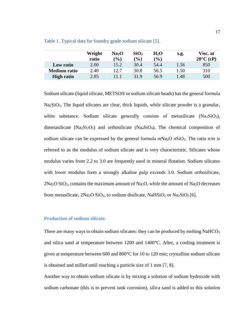
Sodium silicate is water soluble glass available from suppliers in a wide range of types

specified by the silica (SiO2), soda (Na2O) and water content (Table 1). Manufacturer’s

data sheets specify the “weight ratio” of silica to soda, the water percentage and the

viscosity. For foundry use, sodium silicates with ratios between 2 and 3 and water content

around 56% are usually used. Sodium silicate can be hardened in a number of ways: by

adding weak acids (CO2 gas or organic esters), by adding various powders (di-calcium

silicate, anhydrite, etc.) or by removing water [5].

17

Table 1. Typical data for foundry grade sodium silicate [5].

Weight

ratio

Na2O

(%)

SiO2

(%)

H2O

(%)

s.g. Visc. at

20°C (cP)

Low ratio 2.00 15.2 30.4 54.4 1.56 850

Medium ratio 2.40 12.7 30.8 56.5 1.50 310

High ratio 2.85 11.1 31.9 56.9 1.48 500

Sodium silicate (liquid silicate, METSO® or sodium silicate beads) has the general formula

Na2SiO3. The liquid silicates are clear, thick liquids, while silicate powder is a granular,

white substance. Sodium silicate generally consists of metasilicate (Na2SiO3),

dimetasilicate (Na2Si2O5) and orthosilicate (Na4SiO4). The chemical composition of

sodium silicate can be expressed by the general formula mNa2O nSiO2. The ratio n/m is

referred to as the modulus of sodium silicate and is very characteristic. Silicates whose

modulus varies from 2.2 to 3.0 are frequently used in mineral flotation. Sodium silicates

with lower modulus form a strongly alkaline pulp exceeds 3.0. Sodium orthosilicate,

2Na2O SiO2, contains the maximum amount of Na2O, while the amount of Na2O decreases

from metasilicate, 2Na2O SiO2, to sodium disilicate, NaHSiO2 or Na2SiO5 [6].

Production of sodium silicate.

There are many ways to obtain sodium silicates: they can be produced by melting NaHCO3

and silica sand at temperature between 1200 and 1400°C. After, a cooling treatment is

given at temperature between 600 and 800°C for 10 to 120 min; crystalline sodium silicate

is obtained and milled until reaching a particle size of 1 mm [7, 8].

Another way to obtain sodium silicate is by mixing a solution of sodium hydroxide with

sodium carbonate (this is to prevent tank corrosion), silica sand is added to this solution

18

and passed to an autoclave, which is kept at a temperature between 225 and 245°C and

maintained at a pressure between 2.7 and 3.2 MPa. The mixture is left in the autoclave for

about 30 min; once the product is cooled and the pressure is restored to the atmospheric

pressure, the obtained product can be diluted to avoid the silicate crystallization [9, 10].

Another process to obtain sodium silicate is by reacting silica sand with a sodium

hydroxide solution in an autoclave maintaining a temperature between 180 and 240°C and

a pressure from 1.0 to 3.0 MPa; the solution is treated in the spray-drying with hot air from

200 to 300°C for 10 to 20 s and a temperature of exit gas leaving the spray-drying zone

from 90 to 130°C, to form an amorphous sodium silicate powder having a water content of

15 to 23 wt%. Sodium silicate powder is introduced into a rotary furnace with

countercurrent hot air at a temperature form 250 to 500°C for 60 min; the amorphous

sodium silicate emerging from the rotary furnace is milled until reach a size of 0.1 to 12

mm [11].

Sodium silicate can be also produced by melting at high temperatures a mixture of sodium

carbonate (Na2CO3) and specially selected silica sand. The resulting product is an

amorphous crystal (primary glass) which can be dissolved to produce different types of

solutions. In dry form is presented as tablets and it is anhydrous [12].

Additionally sodium silicate can be produced from silica sand and soda ash in a process

similar to that of the glass manufacture, except that the sodium silicates are water soluble

and glass is not. The two raw materials are melted at 2,450°C in an open-heart furnace.

The melt is removed, cooled, crushed, and dissolved under pressure with steam [13].

19

Reactions:

In summary, sodium silicate can be produced by the following reactions:

2NaHCO3 + SiO2(s) ∆→ Na2SiO3 + H2O + 2CO2(g)

Na2CO3 + SiO2(s) ∆→ Na2SiO3 + CO2(g)

2NaOH + SiO2(s) ∆→ Na2SiO3 + H2O

Sodium silicate applications.

Sodium silicates are a group of chemicals used in industry as adhesives, lower carbon

cements, cleaning compounds, deflocculants, protective coatings, soaps and detergents,

silica-type catalysts and gels, pigments, paper adhesives, etc. [6, 13].

Lower carbon footprint cements.

The demand of cement has been increasing due to increased infra-structural activities of

the world. In recent years, lower carbon footprint cements (geopolymers) has attracted

considerable attention among these binders because of its early compressive strength, low

permeability, good chemical resistance and excellent fire resistance behavior [14]. In this

respect, geopolymers are an alternative cementitious binder, comprising of an alkali-

activated fly ash, and they have been considered as a substitute for Ordinary Portland

Cement (OPC). The cement hardens at room temperatures and provides compressive

strengths of 20 MPa after 4 hours and up to 70-100 MPa after 28 days [15]. In addition,

studies that have been completed on geopolymer concretes indicate that there is a potential

for 25-70% reduction in greenhouse gas emissions [16, 17].

20

HYPOTHESIS AND OBJECTIVES

Hypothesis.

Rich silica sands from the region could be chemical and thermally investigated to produce

solid sodium silicate, with the characteristics to develop low carbon footprint cements.

A detailed study to synthesize sodium silicate by different chemical routes allow to

choosing the most efficient route.

General objective.

To establish an efficient synthesis route for the production of solid sodium silicate from

local silica sands banks.

Specific objectives.

- Obtain samples of different silica sand banks.

- Perform a granulometric analysis of silica sands.

- Characterize silica sands by fluorescence and X-ray diffraction techniques, optical

and scanning microscopies, Raman spectroscopy and thermal analysis.

- Experiment with different chemical processes for obtaining sodium silicate, in

order to choose the optimum.

- Characterize the products through techniques: X-ray diffraction, scanning electron

microscopy, Raman and infrared spectroscopies.

21

CHAPTER 2: EXPERIMENTAL METHODOLOGY

This chapter is conceived to know the different experimental techniques, procedure and

equipment used in this work, the preparation techniques and the conditions under which

each was developed.

Fluorescence and X-ray diffractions.

A given substance always produces a characteristic diffraction pattern, whether that the

substance is present in the pure state or as one constituent of a mixture of substances. This

fact is the basis for the diffraction method of chemical analysis. Qualitative analysis for a

particular substance is accomplished by identification of the pattern of that substance.

Quantitative analysis is also possible, because the intensities of the diffraction lines due to

one constituent of a mixture depend on the proportion of that constituent in the specimen.

Diffraction analysis is useful whenever it is necessary to know the state of chemical

combination of the elements involved or the particular phases in which they are present.

As a result, the diffraction method has been widely applied for the analysis of such

materials as ores, clays, refractories, alloys, corrosion products, wear products, industrial

dusts, etc. Compared with ordinary chemical analysis, the diffraction method has the

additional advantages that it is usually much faster, requires only a very small sample, and

is non-destructive [18].

22

X-ray diffraction.

Max von Laue, in 1912, discovered that crystalline substances act as three-dimensional

diffraction gratings for X-ray wavelengths similar to the spacing of planes in a crystal

lattice. X-ray diffraction is a technique for the study of crystal structures and atomic

spacing [19].

X-ray diffraction is based on constructive interference of monochromatic X-rays and a

crystalline sample. These X-rays are generated by a cathode ray tube, filtered to produce

monochromatic radiation, collimated to concentrate, and directed toward the sample [19,

20]. The interaction of the incident rays with the sample produces constructive interference

(and a diffracted ray) when conditions satisfy Bragg's Law (nλ=2d sin θ), Figure 1. This

law relates the wavelength of electromagnetic radiation to the diffraction angle and the

lattice spacing in a crystalline sample. These diffracted X-rays are then detected, processed

and counted. By scanning the sample through a range of 2θ angles, all possible diffraction

directions of the lattice should be attained due to the random orientation of the powdered

material. Conversion of the diffraction peaks to d-spacings allows identification of the

mineral because each mineral has a set of unique d-spacings. Typically, this is achieved by

comparison of d-spacings with standard reference patterns [19, 21].

23

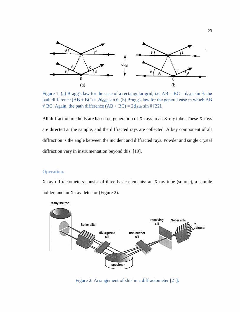
Figure 1: (a) Bragg's law for the case of a rectangular grid, i.e. AB = BC = d(hkl) sin θ: the

path difference (AB + BC) = 2d(hkl) sin θ. (b) Bragg's law for the general case in which AB

≠ BC. Again, the path difference (AB + BC) = 2d(hkl) sin θ [22].

All diffraction methods are based on generation of X-rays in an X-ray tube. These X-rays

are directed at the sample, and the diffracted rays are collected. A key component of all

diffraction is the angle between the incident and diffracted rays. Powder and single crystal

diffraction vary in instrumentation beyond this. [19].

Operation.

X-ray diffractometers consist of three basic elements: an X-ray tube (source), a sample

holder, and an X-ray detector (Figure 2).

Figure 2: Arrangement of slits in a diffractometer [21].

(a) (b

)

24

X-rays are generated in a cathode ray tube by heating a filament to produce electrons,

accelerating the electrons toward a target by applying a voltage, and bombarding the target

material with electrons. When electrons have sufficient energy to dislodge inner shell

electrons of the target material, characteristic X-ray spectra are produced. These spectra

consist of several components, the most common being Kα and Kβ. Kα consists, in part, of

Kα1 and Kα2. Kα1 has a slightly shorter wavelength and twice the intensity as Kα2 (Figure

3). The specific wavelengths are characteristic of the target material (Cu, Fe, Mo, and Cr).

Figure 3: Illustration of the process of inner-shell ionization and the subsequent emission

of a characteristic X-ray: (a) an incident electron ejects a K shell electron from an atom,

(b) leaving a hole in the K shell; (c) electron rearrangement occurs, resulting in the emission

of an X-ray photon [21].

25

Filtering, by foils or crystal monochrometers, is required to produce monochromatic X-

rays needed for diffraction. Kα1 and Kα2 are sufficiently close in wavelength such that a

weighted average of the two is used. Copper is the most common target material for single-

crystal diffraction, with CuKα radiation = 1.5418Å. These X-rays are collimated and

directed onto the sample. As the sample and detector are rotated, the intensity of the

reflected X-rays is recorded. When the geometry of the incident X-rays impinging the

sample satisfies the Bragg’s Equation, constructive interference occurs and a peak in

intensity occurs. A detector records and processes this X-ray signal and converts the signal

to a count rate which is then output to a device such as a printer or computer monitor [19].

Sample preparation and equipment specifications.

For silica sand samples no preparation was done because they were already in powder

form; in the case of sodium silicate samples, a reduction in size was required, which was

made in a porcelain mortar.

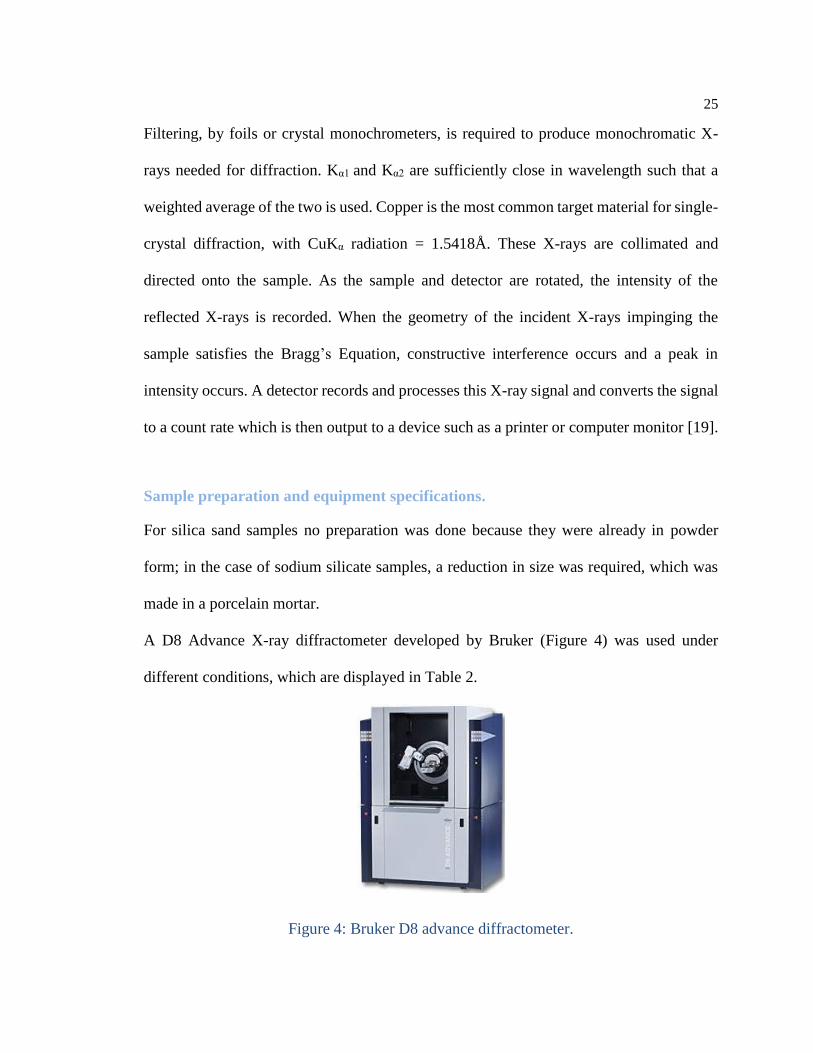
A D8 Advance X-ray diffractometer developed by Bruker (Figure 4) was used under

different conditions, which are displayed in Table 2.

Figure 4: Bruker D8 advance diffractometer.

26

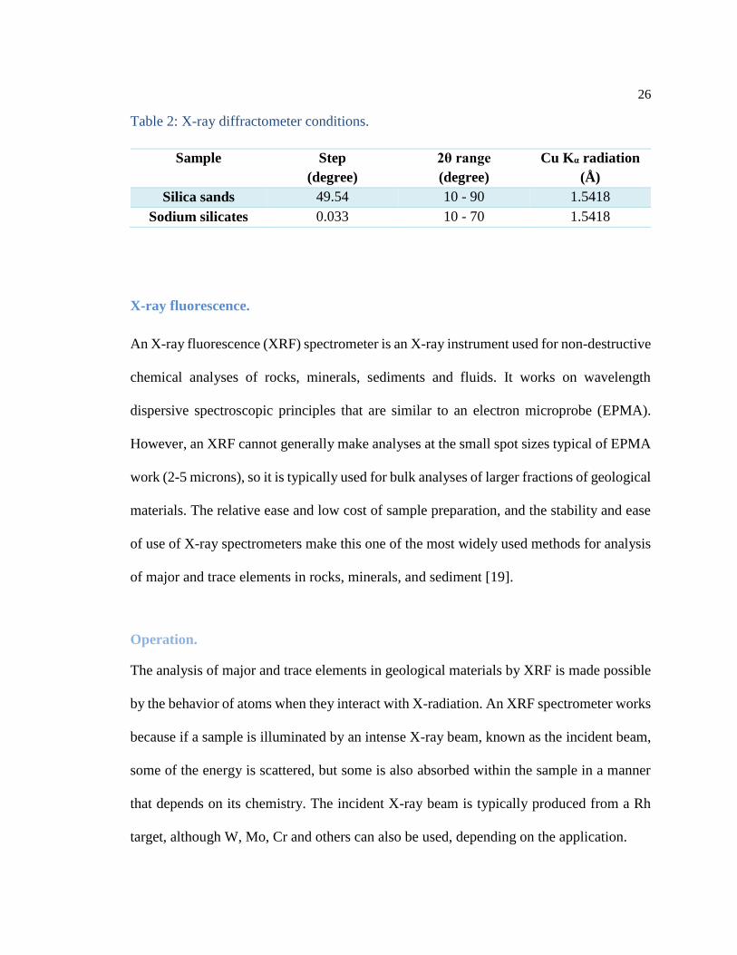
Table 2: X-ray diffractometer conditions.

Sample Step

(degree)

2θ range

(degree)

Cu Kα radiation

(Å)

Silica sands 49.54 10 - 90 1.5418

Sodium silicates 0.033 10 - 70 1.5418

X-ray fluorescence.

An X-ray fluorescence (XRF) spectrometer is an X-ray instrument used for non-destructive

chemical analyses of rocks, minerals, sediments and fluids. It works on wavelength

dispersive spectroscopic principles that are similar to an electron microprobe (EPMA).

However, an XRF cannot generally make analyses at the small spot sizes typical of EPMA

work (2-5 microns), so it is typically used for bulk analyses of larger fractions of geological

materials. The relative ease and low cost of sample preparation, and the stability and ease

of use of X-ray spectrometers make this one of the most widely used methods for analysis

of major and trace elements in rocks, minerals, and sediment [19].

Operation.

The analysis of major and trace elements in geological materials by XRF is made possible

by the behavior of atoms when they interact with X-radiation. An XRF spectrometer works

because if a sample is illuminated by an intense X-ray beam, known as the incident beam,

some of the energy is scattered, but some is also absorbed within the sample in a manner

that depends on its chemistry. The incident X-ray beam is typically produced from a Rh

target, although W, Mo, Cr and others can also be used, depending on the application.

27

When this primary X-ray beam illuminates the sample, it is said to be excited. The excited

sample in turn emits X-rays along a spectrum of wavelengths characteristic of the types of

atoms present in the sample (Figure 5). The atoms in the sample absorb X-ray energy by

ionizing, ejecting electrons from the lower (usually K and L) energy levels. The ejected

electrons are replaced by electrons from an outer, higher energy orbital. When this happens,

energy is released due to the decreased binding energy of the inner electron orbital

compared with an outer one. This energy release is in the form of emission of characteristic

X-rays indicating the type of atom present. If a sample has many elements present, as is

typical for most minerals and rocks, the use of a wavelength dispersive spectrometer much

like that in an EPMA allows the separation of a complex emitted X-ray spectrum into

characteristic wavelengths for each element present. Various types of detectors (gas flow

proportional and scintillation) are used to measure the intensity of the emitted beam. The

flow counter is commonly utilized for measuring long wavelength (>0.15 nm) X-rays that

are typical of K spectra from elements lighter than Zn. The scintillation detector is

commonly used to analyze shorter wavelengths in the X-ray spectrum (K spectra of

element from Nb to I; L spectra of Th and U). X-rays of intermediate wavelength (K spectra

produced from Zn to Zr and L spectra from Ba and the rare earth elements) are generally

measured by using both detectors in tandem. The intensity of the energy measured by these

detectors is proportional to the abundance of the element in the sample. The exact value of

this proportionality for each element is derived by comparison to mineral or rock standards

whose composition is known from prior analyses by other techniques [18, 19].

28

Figure 5: Fluorescent X-ray spectroscopy [18].

Sample preparation and equipment specifications.

Silica sand samples were dried at 100°C, pulverized and then compressed into tablets.

The XRF diffractometer used for this work was a Cubix XRF Dy699 developed by Philips.

The conditions used are displayed in Table 3 .

Table 3: X-ray fluorescence diffractometer.

Time 45 s per sample

Operation temperature 36.5°C

Source 50 kV 4 mA

X-ray tube power 200 W

Tube target Sc

29

Optical microscope.

Microscopes are instruments designed to produce magnified images of small objects. The

microscope must accomplish three tasks: produce a magnified image of the specimen,

separate the details in image, and render the details visible to the human eye or camera.

This group of instruments includes not only multiple-lens designs with objectives and

condensers, but also very simple single lens devices that are often hand-held, such as a

magnifying glass [23].

Components.

Optical microscopes (Figure 6) are designed to provide a magnified two-dimensional

image that can be focused axially in successive focal planes, thus enabling a thorough

examination of specimen fine structural detail in both two and three dimensions.

Most microscopes provide a translation mechanism attached to the stage that allows the

microscopist to accurately position, orient, and focus the specimen to optimize

visualization and recording of images. The intensity of illumination and orientation of light

pathways throughout the microscope can be controlled with strategically placed

diaphragms, mirrors, prisms, beamsplitters, and other optical elements to achieve the

desired degree of brightness and contrast in the specimen [23].

30

Lenses.

The term lens is the common name given to a component of glass or transparent plastic

material, usually circular in diameter, which has two primary surfaces that are ground and

polished in a specific manner designed to produce either a convergence or divergence of

light passing through the material. The optical microscope forms an image of a specimen

placed on the stage by passing light from the illuminator through a series of glass lenses

and focusing this light either into the eyepieces, on the film plane in a traditional camera

system, or onto the surface of a digital image sensor [23].

Illumination.

Sophisticated and well-equipped microscopes fail to yield excellent images due to incorrect

use of the light source, which usually leads to inadequate sample illumination. When

optimized, illumination of the specimen should be bright, glare-free, and evenly dispersed

in the field of view.

There are numerous light sources available to illuminate microscopes, both for routine

observation and critical photomicrography. A most common light source, because of its

low cost and long life, is the 50 or 100 watt tungsten halogen lamp as illustrated at the base

of the microscope diagram in Figure 6, which also details the optical pathways in a typical

modern transmitted light microscope [23].

31

Figure 6: Microscope optical components [23].

Equipment specifications.

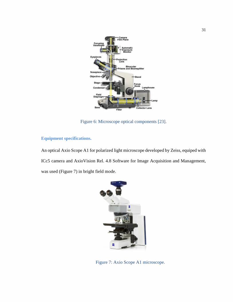
An optical Axio Scope A1 for polarized light microscope developed by Zeiss, equiped with

ICc5 camera and AxioVision Rel. 4.8 Software for Image Acquisition and Management,

was used (Figure 7) in bright field mode.

Figure 7: Axio Scope A1 microscope.

32

Scanning electron microscopy.

The scanning electron microscope (SEM) permits the observation and characterization of

heterogeneous organic and inorganic materials on a nanometer (nm) to micrometer (µm)

scale. It is one of the most versatile instruments available for the examination and analysis

of the microstructural characteristics of solid objects [24]. The signals that derive from

electron-sample interactions reveal information about the sample including external

morphology (texture), chemical composition, and crystalline structure and orientation of

materials making up the sample [25].

The scanning electron microscope has many advantages over traditional microscopes. The

SEM has a large depth of field, which allows more of a specimen to be in focus at one time.

The SEM also has much higher resolution, so closely spaced specimens can be magnified

at much higher levels. Because the SEM uses electromagnets rather than lenses, the

researcher has much more control in the degree of magnification. All of these advantages,

as well as the actual strikingly clear images, make the scanning electron microscope one

of the most useful instruments in research today [26].

System components.

While the variations from one model to the next are seemingly endless, all SEMs share the

same basic parts, which can be seen in Figure 8.

33

Figure 8: The two major parts of the SEM, the electron column and the electronics console

[24].

Electron gun.

It produces the steady stream of electrons necessary for SEMs to operate. Electron guns

are typically one of two types. Thermionic guns, which are the most common type, apply

thermal energy to a filament (usually made of tungsten, which has a high melting point) to

take electrons away from the gun and toward the specimen under examination. Field

emission guns, on the other hand, create a strong electrical field to pull electrons away from

the atoms they are associated with. Electron guns are located either at the very top or at the

very bottom of an SEM and fire a beam of electrons at the object under examination [27]

34

Lenses.

Just like optical microscopes, SEMs use lenses to produce clear and detailed images. The

lenses in these devices, however, work differently. For one thing, they are not made of

glass. Instead, the lenses are made of magnets capable of bending the path of electrons. By

doing so, the lenses focus and control the electron beam, ensuring that the electrons end up

precisely where they need to go [27].

Sample chamber.

The sample chamber of an SEM is where the specimen that is examined is placed. Because

the specimen must be kept extremely still for the microscope to produce clear images, the

sample chamber must be very sturdy and insulated from vibration. The sample chambers

of a SEM do more than keep a specimen still. They also manipulate the specimen, placing

it at different angles and moving it [27].

Detectors.

These devices detect the various ways that the electron beam interacts with the sample

object. For instance, Everhart-Thornley detectors register secondary electrons, which are

electrons dislodged from the outer surface of a specimen. These detectors are capable of

producing the most detailed images of an object's surface. Other detectors, such as

backscattered electron detectors and X-ray detectors, can determine the composition of a

substance [27].

35

Vacuum chamber.

SEMs require a vacuum to operate. Without a vacuum, the electron beam generated by the

electron gun would encounter constant interference from air particles in the atmosphere.

Not only would these particles block the path of the electron beam, they would also be

knocked out of the air and onto the specimen, which would distort the surface of the

specimen [27].

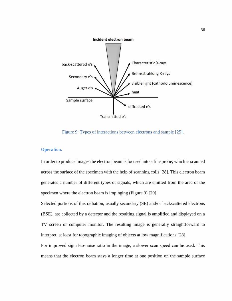
Electron-sample interactions.

Electrons accelerated onto a material result in a number of interactions with the atoms of

the target sample. Accelerated electrons can pass through the sample without interaction,

undergo elastic scattering and can be inelastically scattered (Figure 9). Elastic and inelastic

scattering result in a number of signals that are used for imaging, quantitative and semi-

quantitative information of the target sample and generation of an X-ray source. Typical

signals used for imaging include secondary electrons (SE), backscattered electrons (BSE),

cathodoluminescence (CL), Auger electrons and characteristic X-rays. Quantitative and

semiquantitative analyses of materials as well as element mapping typically utilize

characteristic X-rays [25].

36

Figure 9: Types of interactions between electrons and sample [25].

Operation.

In order to produce images the electron beam is focused into a fine probe, which is scanned

across the surface of the specimen with the help of scanning coils [28]. This electron beam

generates a number of different types of signals, which are emitted from the area of the

specimen where the electron beam is impinging (Figure 9) [29].

Selected portions of this radiation, usually secondary (SE) and/or backscattered electrons

(BSE), are collected by a detector and the resulting signal is amplified and displayed on a

TV screen or computer monitor. The resulting image is generally straightforward to

interpret, at least for topographic imaging of objects at low magnifications [28].

For improved signal-to-noise ratio in the image, a slower scan speed can be used. This

means that the electron beam stays a longer time at one position on the sample surface

37

before moving to the next. This gives a higher detected signal and increased signal-to noise

ratio [29].

Sample preparation and equipment specifications.

Silica sand samples were milled for five minutes using a SPEX 8000M mixer/mill in order

to reduce their size (see Milling in chapter 2). In the case of sodium silicate samples, they

were prepared as it was mentioned in the X-ray diffraction section.

For the development of this work, two SEMs were used: for silica sand samples a JEOL

5800 LV (Figure 10a) and for sodium silicate samples a Hitachi SU3500 (Figure 10b); both

microscopes were operated under 15 kV.

(a) (b)

Figure 10: Scanning electron microscopes. (a) JEOL 5800LV, (b) Hitachi SU3500.

38

Thermal analysis.

There are many ways to characterize samples by scanning thermoanalytical techniques

such as: differential thermal analysis (DTA), differential scanning calorimetry (DSC),

dilatometry, and thermogravimetric analysis (TGA). Although there are a myriad of

devices used to measure the temperature of an object, thermal analysis instruments

predominantly use thermocouples, platinum resistance thermometers and thermistors [30].

Differential thermal analysis (DTA).

The temperature difference between a reactive sample and a non-reactive reference is

determined as a function of time, providing useful information about the temperatures,

thermodynamics and kinetics of reactions [30].

39

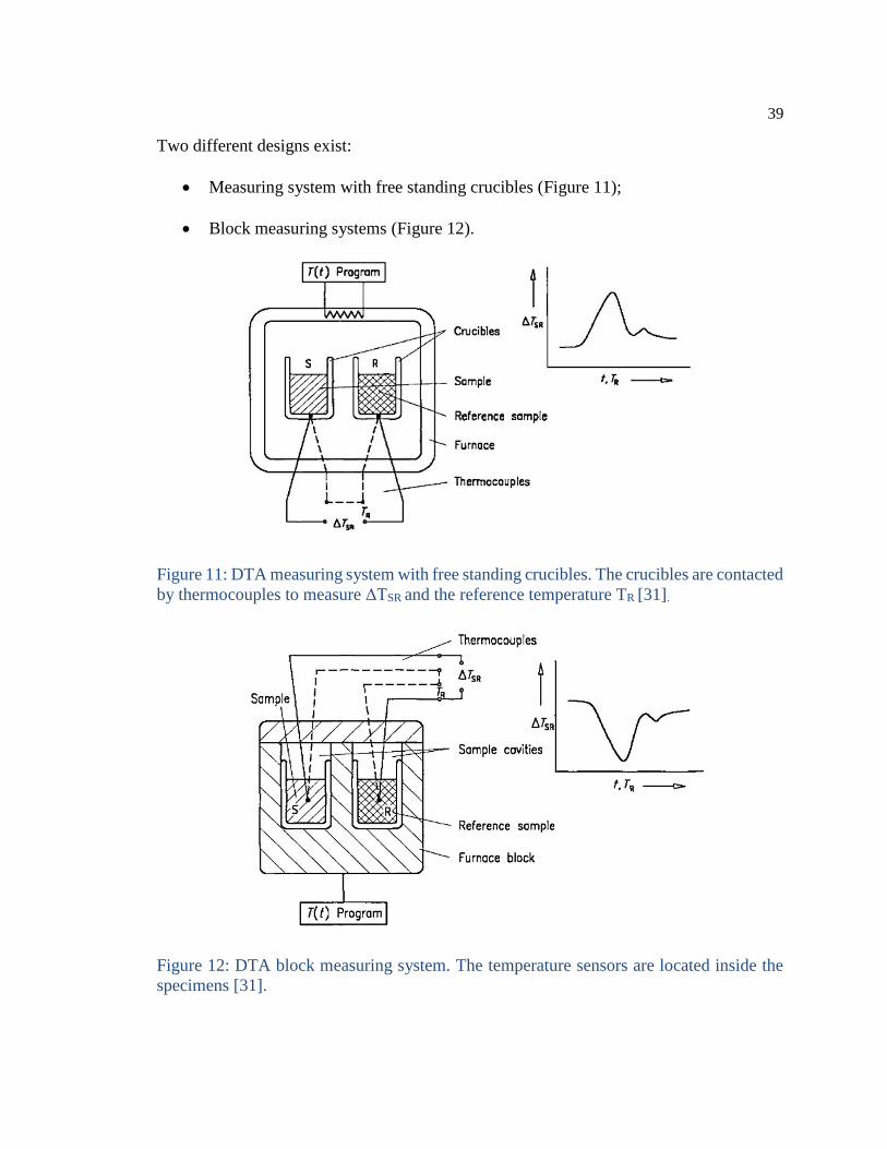
Two different designs exist:

Measuring system with free standing crucibles (Figure 11);

Block measuring systems (Figure 12).

Figure 11: DTA measuring system with free standing crucibles. The crucibles are contacted

by thermocouples to measure ΔTSR and the reference temperature TR [31].

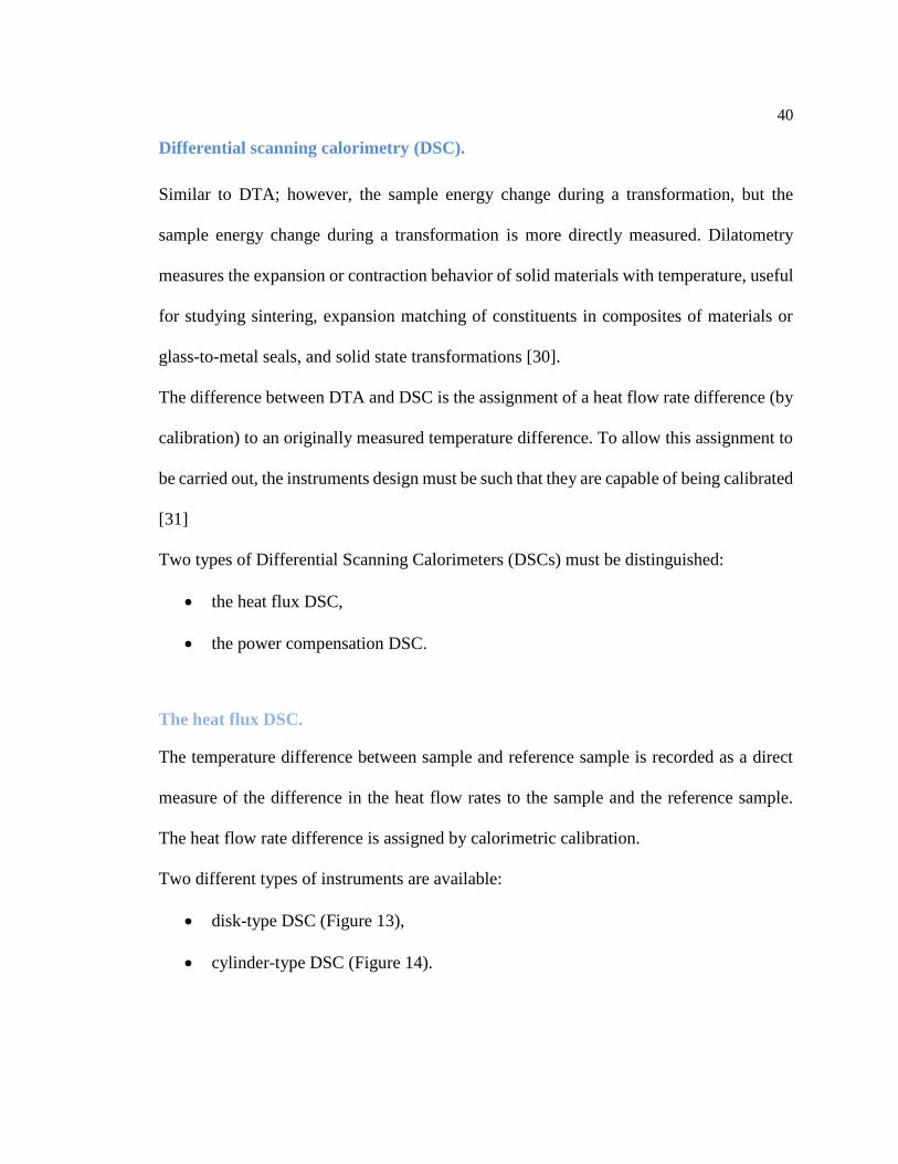
Figure 12: DTA block measuring system. The temperature sensors are located inside the

specimens [31].

40

Differential scanning calorimetry (DSC).

Similar to DTA; however, the sample energy change during a transformation, but the

sample energy change during a transformation is more directly measured. Dilatometry

measures the expansion or contraction behavior of solid materials with temperature, useful

for studying sintering, expansion matching of constituents in composites of materials or

glass-to-metal seals, and solid state transformations [30].

The difference between DTA and DSC is the assignment of a heat flow rate difference (by

calibration) to an originally measured temperature difference. To allow this assignment to

be carried out, the instruments design must be such that they are capable of being calibrated

[31]

Two types of Differential Scanning Calorimeters (DSCs) must be distinguished:

the heat flux DSC,

the power compensation DSC.

The heat flux DSC.

The temperature difference between sample and reference sample is recorded as a direct

measure of the difference in the heat flow rates to the sample and the reference sample.

The heat flow rate difference is assigned by calorimetric calibration.

Two different types of instruments are available:

disk-type DSC (Figure 13),

cylinder-type DSC (Figure 14).

41

Figure 13: Disc-type DSC [31].

Disk-type DSC.

The crucibles with the specimens are positioned on a disk (made of metal, ceramics or the

like). The temperature difference ΔTSR between the specimens is measure with temperature

sensors integrated in the disk or contacting the disk surface [31].

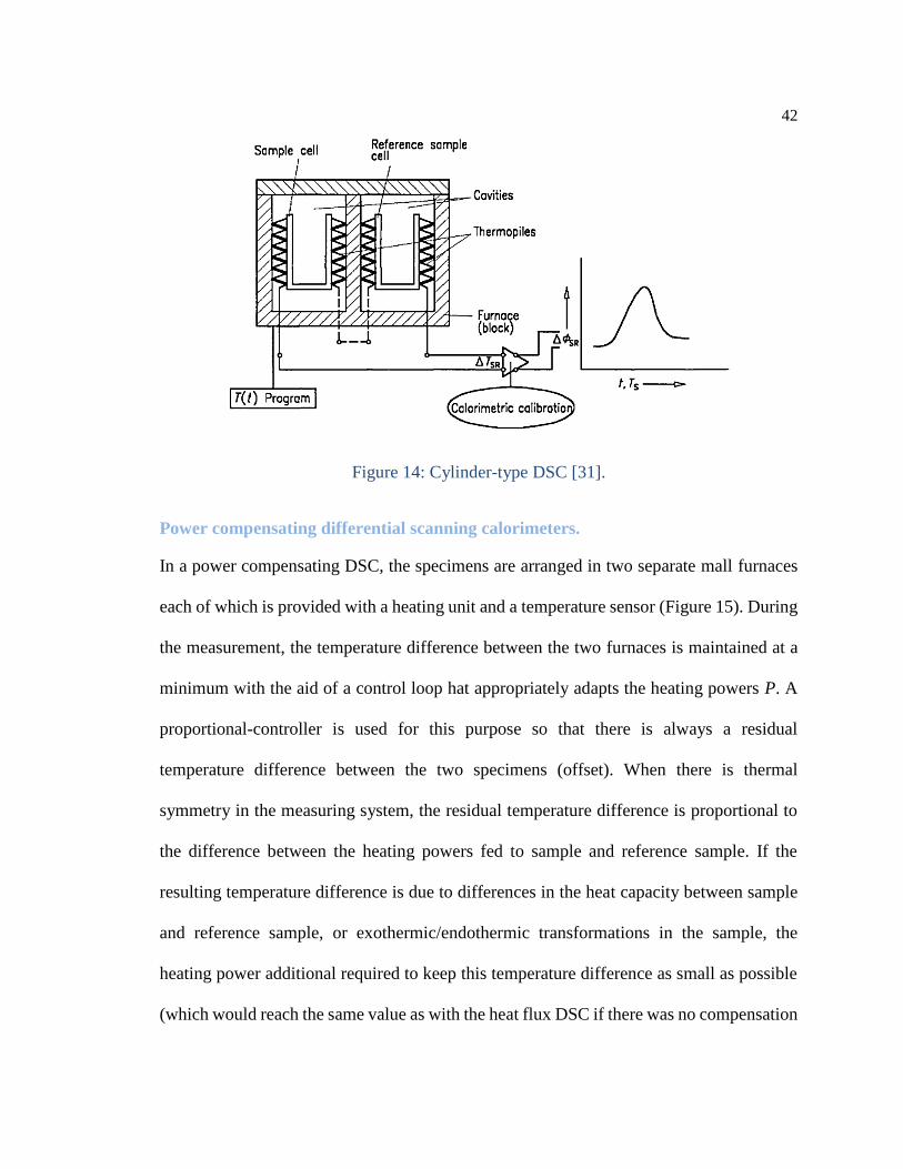
Cylinder-type DSC.

The furnace is provided with two (or more) cylindrical cavities. They take up hollow

cylinders whose bottoms are closed (cells) and in which the specimens are placed directly

or in suitable crucibles. Thermopiles or thermoelectrical semi-conducting sensors are

arranged between the hollow cylinder and the furnace, which measure the temperature

difference between the two hollow cylinders, which is registered as the temperature

difference ΔTSR between the sample and reference sample. Variants of the design: the two

hollow cylinders are arranged side by side in the furnace directly connected through one or

several thermopiles. There are also other DSC designs whose construction features are

between those disk-type and cylinder type DSC [31].

42

Figure 14: Cylinder-type DSC [31].

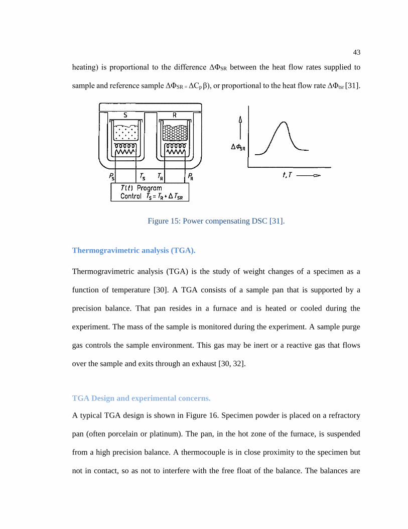
Power compensating differential scanning calorimeters.

In a power compensating DSC, the specimens are arranged in two separate mall furnaces

each of which is provided with a heating unit and a temperature sensor (Figure 15). During

the measurement, the temperature difference between the two furnaces is maintained at a

minimum with the aid of a control loop hat appropriately adapts the heating powers P. A

proportional-controller is used for this purpose so that there is always a residual

temperature difference between the two specimens (offset). When there is thermal

symmetry in the measuring system, the residual temperature difference is proportional to

the difference between the heating powers fed to sample and reference sample. If the

resulting temperature difference is due to differences in the heat capacity between sample

and reference sample, or exothermic/endothermic transformations in the sample, the

heating power additional required to keep this temperature difference as small as possible

(which would reach the same value as with the heat flux DSC if there was no compensation

43

heating) is proportional to the difference ΔΦSR between the heat flow rates supplied to

sample and reference sample ΔΦSR = ΔCp β), or proportional to the heat flow rate ΔΦtsr [31].

Figure 15: Power compensating DSC [31].

Thermogravimetric analysis (TGA).

Thermogravimetric analysis (TGA) is the study of weight changes of a specimen as a

function of temperature [30]. A TGA consists of a sample pan that is supported by a

precision balance. That pan resides in a furnace and is heated or cooled during the

experiment. The mass of the sample is monitored during the experiment. A sample purge

gas controls the sample environment. This gas may be inert or a reactive gas that flows

over the sample and exits through an exhaust [30, 32].

TGA Design and experimental concerns.

A typical TGA design is shown in Figure 16. Specimen powder is placed on a refractory

pan (often porcelain or platinum). The pan, in the hot zone of the furnace, is suspended

from a high precision balance. A thermocouple is in close proximity to the specimen but

not in contact, so as not to interfere with the free float of the balance. The balances are

44

electronically compensated so that the specimen pan does not move when the specimen

gains or losses weight [30].

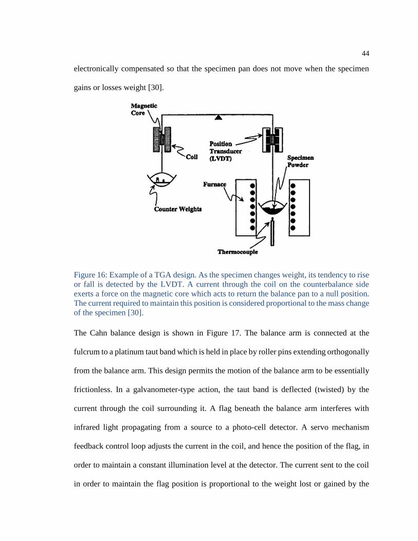
Figure 16: Example of a TGA design. As the specimen changes weight, its tendency to rise

or fall is detected by the LVDT. A current through the coil on the counterbalance side

exerts a force on the magnetic core which acts to return the balance pan to a null position.

The current required to maintain this position is considered proportional to the mass change

of the specimen [30].

The Cahn balance design is shown in Figure 17. The balance arm is connected at the

fulcrum to a platinum taut band which is held in place by roller pins extending orthogonally

from the balance arm. This design permits the motion of the balance arm to be essentially

frictionless. In a galvanometer-type action, the taut band is deflected (twisted) by the

current through the coil surrounding it. A flag beneath the balance arm interferes with

infrared light propagating from a source to a photo-cell detector. A servo mechanism

feedback control loop adjusts the current in the coil, and hence the position of the flag, in

order to maintain a constant illumination level at the detector. The current sent to the coil

in order to maintain the flag position is proportional to the weight lost or gained by the

45

specimen. A dc voltage proportional to this current is provided for external data acquisition.

These balances have a manufacturer’s reported precision of 0.1 µg [30].

Figure 17: Gahn microbalance design [30].

Equipment specifications.

A DSC autosampler (Figure 18) developed by TA Instruments was used. For silica sand

samples the analysis were performed in a range from 25 to 850°C, whereas for the reactions to

produce sodium silicate they were out between 25 and 1100°C; in both of them an air

atmosphere was used.

Figure 18: DSC Autosampler, TA instruments.

46

Thermocouples.

A thermocouple is a device for the measurement of temperature. Its operation is based upon

the finding of Seebeck (1821) [33]. His work showed that a small electric current will flow

in a closed circuit composed of two dissimilar metallic conductors when their junctions are

kept at different temperatures. The electromotive force, emf, produced under these

conditions is known as the Seebeck emf. Their pair of conductors, or thermocouple

elements, which constitutes the thermoelectric circuit is called a thermocouple. Simply

stated, a thermocouple is a device which converts thermal energy to electric energy. The

amount of electric energy produced can be used to measure temperature [33].

Common thermocouple types.

The commonly used thermocouple types are identified by letter dessignations originally

assigned by the Instrument Society of America (ISA) and adopted as an American Standar

in ANSI-C96.1-1964 [34].

B-type.- Pt-30% Rd (+) versus Pt-6%Rd (-).

E-type.- Ni-10%Cr (+) versus constantan1 (-).

J-type.- Iron (+) versus constantan (-).

K-type.- Ni-10%Cr (+) versus Ni-5%(Al, Si) (-)

R-type.- Pt-13%Rd (+) versus Pt (-).

S-type.- Pt-10%Rd (+) versus Pt (-).

1 Constantan is an alloy compound of 55% Cu and 45% Ni (Cu55Ni45)

47

T-type.- Cu (+) versus constantan (-).

T-type thermocouple.

These thermocouples are resistant to corrosion in moist atmospheres and are suitable for

subzero temperature measurements. They have an upper temperature limit of 371 °C and

can be used in a vacuum and oxidizing, reducing, or inert atmospheres. This is the only

thermocouple type for which limits of error are established in the subzero temperature

range [33].

J-type thermocouple.

These thermocouples are suitable for use in vacuum and in oxidizing, reducing, or inert

atmospheres, at temperatures up to 760°C. The rate of oxidation of the iron thermoelement

is rapid above when long life is required at the higher temperatures [33].

K-type thermocouple.

K-type thermocouples are recommended for continuous use in oxidizing or inert

atmospheres at temperatures up to 1260°C. Because their oxidation resistance

characteristics are better than those of other base metal thermocouples, they find widest

use at temperature above 538°C. However, this thermocouple is suitable for temperature

measurements as low as -250°C, although limits of error have been established only for the

temperature range of -18 to 1260°C [33].

48

Sample preparation and equipment specifications.

The reactive mixtures (see “Reaction Procedure” in chapter 3) were placed in the crucibles

and K-type thermocouples were placed in the middle part of the samples.

The following crucibles were used in this work:

- Alumina crucibles.

- Iron crucibles.

- Nickel crucibles.

- Copper crucibles.

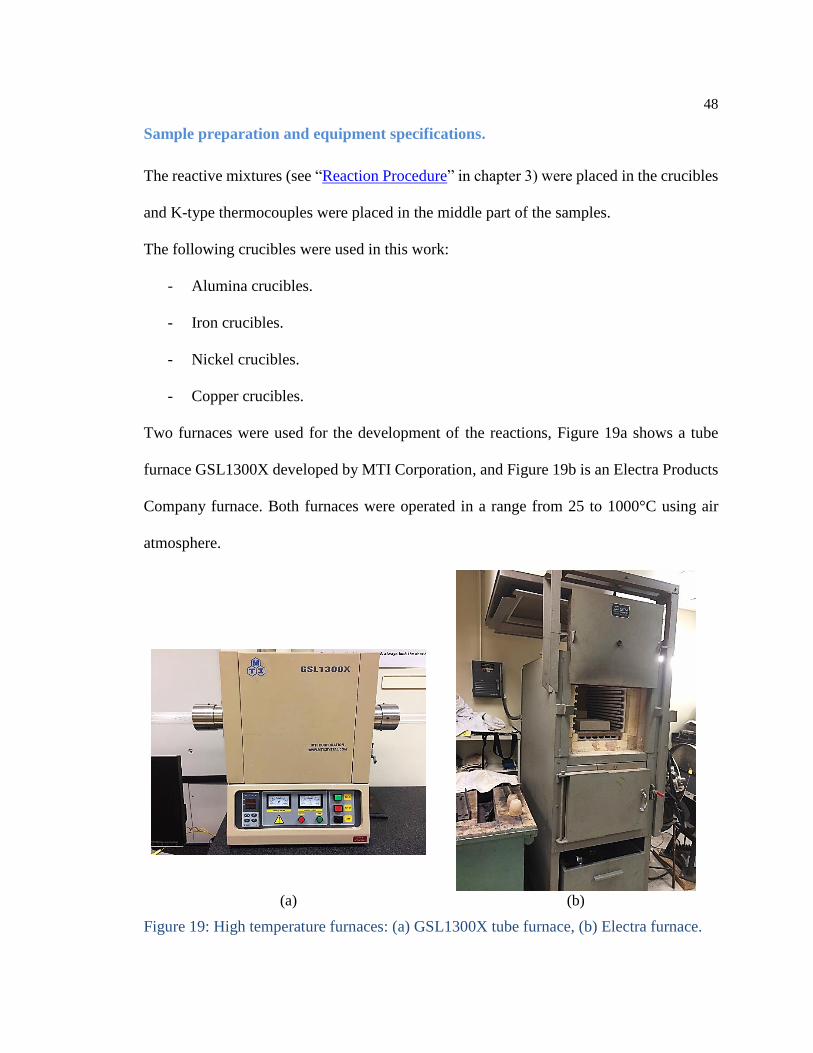
Two furnaces were used for the development of the reactions, Figure 19a shows a tube

furnace GSL1300X developed by MTI Corporation, and Figure 19b is an Electra Products

Company furnace. Both furnaces were operated in a range from 25 to 1000°C using air

atmosphere.

(a) (b)

Figure 19: High temperature furnaces: (a) GSL1300X tube furnace, (b) Electra furnace.

49

In order to collect thermocouples data information, a computer equipped with a National

Instruments “cDAQ-9174” card and a thermocouple input module “NI 9213” were used;

furthermore, a LabView software acquired the information.

Fourier transform infra-red spectroscopy.

Fourier Transform Infra-Red (FTIR) is a diverse molecular spectroscopy technique and

chemical analysis method. While FTIR is frequently used for polymer testing and

pharmaceutical analysis, it can provide qualitative analysis of a wide range of organic and

inorganic samples [35].

Infrared spectroscopy probes molecular motions which involve a change in the dipole

moment. The FTIR technique is based on a Michelson interferometer [36].

Figure 20: Michelson Interferometer [36].

50

Operation.

In a Michelson interferometer (Figure 20), the polychromatic light (S) from the light source

(Globar or tungsten lamp) passes through a beamsplitter (B), where the light is split into

equal parts. Half of the light goes to a fixed mirror (M2) and half of the light goes to a

movable mirror (M1). The light is then reflected off the mirrors and is recombined through

the beamsplitter. At the detector (D), constructive interference will take place if the path

length is the same between the two mirrors. The motion of the mirror leads to a pattern of

destructive and constructive interference as a function of displacement, which is called the

interferogram. A HeNe laser is used to measure the path difference of the moveable mirror

(Connes advantage).

A FTIR spectrometer is a multiplex instrument, which means that all the spectral

information measured simultaneously by the detector. The sensitivity is better because of

the Jacquinot advantage, which allows for a large energy throughput due to the possibility

to use a large aperture.

The absorbance A is defined by the Lambert-Beer equation as:

𝐴 = 𝑙𝑛𝐼0

𝐼= ɛ 𝑐 𝑙

In this equation I is the light intensity after it passes through the probe, I0 is the light

intensity before it passes the probe, ɛ is the absorption coefficient, c is the concentration

and l is the path length probed by the beam [36].

51

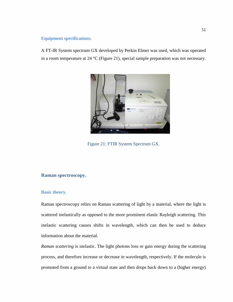
Equipment specifications.

A FT-IR System spectrum GX developed by Perkin Elmer was used, which was operated

in a room temperature at 24 °C (Figure 21), special sample preparation was not necessary.

Figure 21: FTIR System Spectrum GX.

Raman spectroscopy.

Basic theory.

Raman spectroscopy relies on Raman scattering of light by a material, where the light is

scattered inelastically as opposed to the more prominent elastic Rayleigh scattering. This

inelastic scattering causes shifts in wavelength, which can then be used to deduce

information about the material.

Raman scattering is inelastic. The light photons loss or gain energy during the scattering

process, and therefore increase or decrease in wavelength, respectively. If the molecule is

promoted from a ground to a virtual state and then drops back down to a (higher energy)

52

vibrational state, then the scattered photon has less energy than the incident photon, and

therefore a longer wavelength. This is called Stokes scattering. If the molecule is in a

vibrational state to begin with and after scattering is in its ground state, then the scattered

photon has more energy, and therefore a shorter wavelength. This is called anti-Stokes

scattering. Normally in Raman spectroscopy only the Stokes half of the spectrum is used,

due to its greater intensity [37].

Origin of the Raman spectra.

Vibrational transitions can be observed in either Infrared (IR) or Raman spectra. In the

former, the absorption of infrared light by the sample as a function of frequency is

measured. The origin of Raman spectra is markedly different from that of IR spectra. In

Raman spectroscopy, the sample is irradiated by intense laser beams in the UV-Visible

region and the scattered light is usually observed in the direction perpendicular to the

incident beam (Figure 22).

Figure 22: Types of Raman scattering signals.

53

The scattered light consists of two types: one called Rayleigh scattering is strong and has

the same frequency as the incident beam (v0) and the other called Raman scattering, is very

weak and has frequencies v0 ± vm , which is a vibrational frequency of a molecule. The v0 -

vm and v0 + vm lines are called the Stokes and anti-Stokes, respectively [38].

Raman active modes.

For a mode to be Raman active it must involve a change in the polarizability, α of the

molecule (𝑑α

𝑑𝑞)

𝑒≠ 0, where q is the normal coordinate and “e” the equilibrium position.

This is known as spectroscopic selection. The spectroscopic selection rule for infrared

spectroscopy is that only transitions that cause a change in dipole moment can be observed.

Because this relates to different vibrational transitions than in Raman spectroscopy, the

two techniques are complementary [37].

Raman equipment design.

Five major components make up the commercially available Raman spectrometer. These

consist on the following:

- Excitation source, which is generally a continuous wave (CW) gas laser.

- Sample holder [38].

- Grating and filters [37].

- Detection system [38].

54

Excitation source.

Lasers are ideal excitation sources for Raman spectroscopy, mainly due to the following

characteristics: 1) Laser beams are highly monochromatic, 2) Laser beams have small

diameter (1-2 mm) which can be reduced to 0.1 mm using simple lens systems [38].

Sample holder.

Raman can capture data from a sample contained in plastic or other materials that are

optically transparent to the wavelengths of interest. And unlike IR spectroscopy, which

falls spectrally within the water window, Raman spectroscopy can be used to capture data

on aqueous samples or samples with high moisture content [39].

Grating.

This diffracts the scattered light into a spectrum. The grating density affects the spectral

resolution and range, so the spectrometer may have multiple gratings which can be

switched [37].

Filters.

These remove stray light that has been Rayleigh scattered [37].

Detection system.

This collects the spectrum and converts it into electrical signals. It is cooled to reduce

thermal noise [37].

55

Operation.

First the light from the laser is focused on the sample, and then the sample scatters the light.

Most of this scattering is Rayleigh scattering, so has the same wavelength. A small amount

is Raman scattered, changing in wavelength. The filters (chosen according to the

wavelength) remove the Rayleigh scattered light, leaving only that which has undergone

Raman scattering. The grating diffracts the light incident on it. It can be rotated in order to

select different wavelengths. The Charge Couple Device (CCD) detector produces an

electrical signal according to the intensity of the light. This is then passed to a computer

for analysis [37].

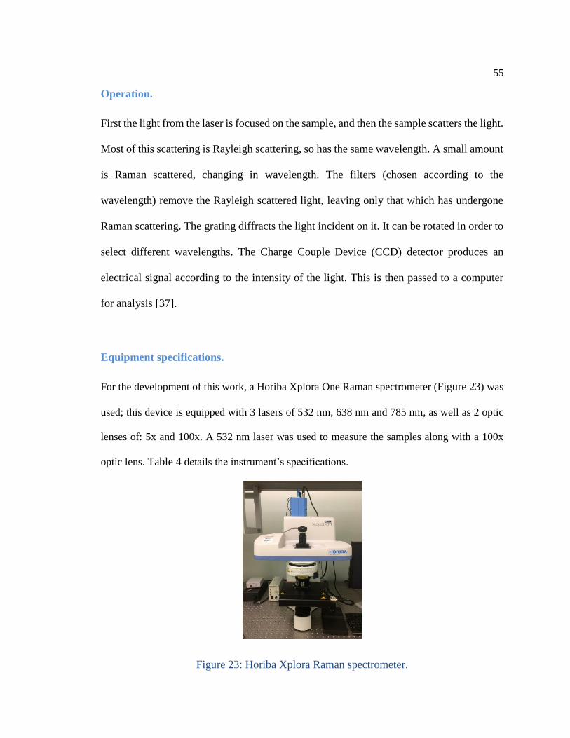
Equipment specifications.

For the development of this work, a Horiba Xplora One Raman spectrometer (Figure 23) was

used; this device is equipped with 3 lasers of 532 nm, 638 nm and 785 nm, as well as 2 optic

lenses of: 5x and 100x. A 532 nm laser was used to measure the samples along with a 100x

optic lens. Table 4 details the instrument’s specifications.

Figure 23: Horiba Xplora Raman spectrometer.

56

Table 4: Raman’s instrument specifications.

Spectral range 100 cm-1 to 3500 cm-1 minimum range in ONE-shot operation

(depending upon laser).

Spectrograph: Imaging flat field spectrometer for use with large area CCD

detector.

High throughput/sensitivity.

Detector: 1024x256 TE air-cooled scientific CCD, USB control, no

maintenance vacuum, 16 bit and up to 1.48 MHz readout speed.

Offering improved sensitivity and fast Raman acquisition.

Microscope Materials/clinical light microscope. Optimized for stability

with high quality optics and ergonomic design. Includes Kohler

illumination for transmission and reflection illumination, abbe

condenser, 10x and 50x objectives (100x objective optional).

Confocal sampling Rugged confocal spatial filtering, offering maximum 1 µm

x1µm lateral resolution for micron scale Raman analysis and

imaging (where 100x objective used).

Monitor Desktop PC with monitor, keyboard and mouse, pre-loaded

with Windows 7TM 32-bit and LabSpec 6 spectral software

suite.

57

Samples.

In order to select the most effective sample, 9 different silica sand samples were analyzed,

each sample corresponds to a different silica sand bank except for the sample “CS”, which

corresponds to a commercial silica sand from US Silica Company.

Silica sands:

Samalayuca

o Samalayuca 1 “S1”

o Samalayuca 2 “S2”

Cuervo

o Cuervo 1 “C1

o Cuervo 2 “C2”

o Cuervo 3 “C3”

Lajas

o Lajas 1 “L1”

o Lajas 2 “L2”

o Lajas 3 “L3”

Control Sample “CS”

58

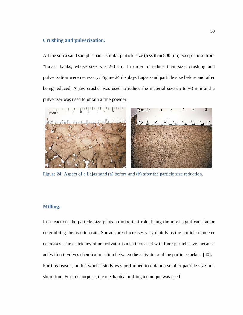
Crushing and pulverization.

All the silica sand samples had a similar particle size (less than 500 µm) except those from

“Lajas” banks, whose size was 2-3 cm. In order to reduce their size, crushing and

pulverization were necessary. Figure 24 displays Lajas sand particle size before and after

being reduced. A jaw crusher was used to reduce the material size up to ~3 mm and a

pulverizer was used to obtain a fine powder.

Figure 24: Aspect of a Lajas sand (a) before and (b) after the particle size reduction.

Milling.

In a reaction, the particle size plays an important role, being the most significant factor

determining the reaction rate. Surface area increases very rapidly as the particle diameter

decreases. The efficiency of an activator is also increased with finer particle size, because

activation involves chemical reaction between the activator and the particle surface [40].

For this reason, in this work a study was performed to obtain a smaller particle size in a

short time. For this purpose, the mechanical milling technique was used.

59

Silica sands were reduced using a SPEX 8000M mixer/mill (Figure 25a) operated at 1600

r.p.m. under an air atmosphere for different milling times. Methanol (MeOH) was added

as a process control agent in order to avoid material agglomeration. A CILAS1180

equipment was employed to determine the particle size of the milled powders (Figure 25b).

This equipment uses the laser diffraction and a CCD camera, which allows, in one single

range, the measure of particles between 0.04 and 2,500 µm. The fine particles are measured

by the diffraction pattern, using Fraunhofer or Mie theory. The coarse particles are

measured using a real-time Fast Fourier Transform of the image obtained with a CCD

camera equipped with a digital signal processing unit (DSP) [41].

(a) SPEX 8000M mixer/mill (b) CILAS 1180

Figure 25: Equipment used to reduce and measure particle size. (a) High energy mixer mill,

(b) CILAS equipment.

60

Reaction procedure.

In order to synthesize sodium silicate, three different reactions were studied and conducted

in this work (Table 5). Before carrying out the reactions, they were simulated in the HSC

Chemical® software with the aim of obtaining their ΔG. A negative ΔG indicates that the

process or chemical reaction proceeds spontaneously in the forward direction; a positive

ΔG indicates that the process proceeds spontaneously in the reverse direction (unfavorable)

and, when ΔG is zero, the process is already in equilibrium, with no net change taking

place over time. For purposes of this work, a negative ΔG is necessary.

Table 5: Reactions to synthesize sodium silicate.

Given name Reaction

M1 2NaHCO3 + SiO2(s)

∆→ Na2SiO3 + H2O + 2CO2(g)

M2 Na2CO3 + SiO2(s)

∆→ Na2SiO3 + CO2(g)

M3 2NaOH + SiO2(s)

∆→ Na2SiO3 + H2O

A stoichiometric study was conducted to obtain the necessary amounts of each reactant for

the reaction properly takes place.

61

Experimental reaction.

Reactions M1 and M2 were carried out using a DSC autosampler, with whose results and

data of the HSC Chemical® software, bulk materials could be produced using a higher

capacity furnace. The sample temperature could be measured in every moment using K-

type thermocouples. A tube furnace was used to obtain heating curves unaltered by the air

presence. The first derivative of these thermograms showed the curvature changes, which

indicated that phase transformations were occurring.

M3 reaction was conducted in two ways: the first one consisted in a soda solution and

silicon dioxide (sand) carried out in a chemical reactor. The second reaction was developed

in a furnace using K-type thermocouples.

62

CHAPTER 3: RESULTS AND DISCUSSION

In this chapter the characterization results of the silica sand banks as well as the synthesis

of sodium silicate will be presented and discussed.

ΔG simulation.

Figure 26 shows the simulation results of each reaction achieved. As can be seen, all the

ΔG values are negative, which means that the reactions described in chapter 2 are able to

succeed. However, this only gives an indication of the temperatures at which it is possible

to work with each reaction.

Figure 26: ΔG simulation results of the different reactions.

200 400 600 800 1000 1200-400

-300

-200

-100

0

100

M1

M2

M3

G

(kJ)

Temperature (°C)

63

SILICA SAND BANKS

Optical microscopy.

Control Sample (CS) micrograph in Figure 27 displays a regular size and morphology.

Figure 28 shows optical micrographs of the sands, which have similar size and

morphology, excluding Lajas sands whose particle size is smaller due to the previous

reduction. All samples have the same roundish appearance.

Control Sample

Figure 27: Control sample micrograph.

Samalayuca 1 Samalayuca 2

Figure 28: Micrographs of the different silica sand banks (continued on

next page).

64

Cuervo 1 Cuervo 2

Cuervo 3 Lajas 1

Lajas 2 Lajas 3

Figure 28: Micrographs of the different silica sand banks (continued from

previous page).

65

Particle size distribution.

Table 6 presents the particle size distribution before milling, obtained by gradation test

using different meshes. The results indicate a highly variation for all the samples except

for CS sample. Cuervo and Lajas silica sand samples have cumulative percentage at the

200 mesh, which means that the particle size for those samples remains between 74 and

149 µm. Samalayuca silica sand samples are between 149 and 177 µm and CS silica sand

sample is between 250 and 400 µm. These results can also be appreciated in Figure 29.

Table 6: Results of particle size distribution (wt %).

Mesh CS S1 S2 C1 C2 C3 L1 L2 L3

40 16.5 0.7 0.0 1.9 1.7 0.0 6.0 3.5 27.6

60 70.2 2.3 2.0 2.8 7.2 8.8 10.0 12.5 8.2

80 12.4 33.0 38.9 21.9 26.4 26.7 15.7 22.5 10.6

100 0.9 43.3 41.0 24.2 23.0 22.4 10.2 11.1 7.2

200 0.0 20.5 17.4 46.4 39.4 40.9 39.6 37.9 41.0

300 0.0 0.2 0.7 2.9 2.3 1.2 18.5 12.5 5.4

Figure 29: Results of mesh distribution.

66

Milling.

In order to not perform unnecessary tests, this study was based on sample “CS”, since

according to the above results, this one has a larger particle size in comparison with the

other silica sand samples.

The results of Figure 30 indicate that 5 min are enough to reduce its particle size; the

particle size reduction is not worth with longer times, there is even an increment at 120

min.

Figure 30: Average "CS" silica sand particle size versus milling time.

Table 7 shows the diameter dispersion at different milling times. As can be observed, with

5 min of milling the 90% of all the sample has an average diameter of 27.68 µm, the 50%

an average diameter of 5.53 µm and the 10% a diameter of 1.06 µm.

0

10

20

30

40

50

60

30

Av

era

ge

(m

)

Milling time (min)1 2 5 10 120

67

Table 7: Diameter dispersion at different milling times.

Milling time

(min)

Diameter at 10%

(µm)

Diameter at 50%

(µm)

Diameter at 90%

(µm)

1 3.52 ± 0.10 35.53 ± 0.46 157.32 ± 1.30

2 2.21 ± 0.01 15.54 ± 0.05 59.41 ± 0.25

5 1.06 ± 0.09 5.53 ± 0.24 27.68 ± 0.96

10 0.98 ± 0.01 4.35 ± 0.13 21.52 ± 0.70

30 0.99 ± 0.01 4.84 ± 0.18 23.00 ± 0.70

120 1.05 ± 0.21 6.96 ± 0.41 31.71 ± 2.15

X-ray diffraction.

Silica sand samples were analyzed by X-ray diffraction. As can be seen in Figure 31 all

samples contain silicon dioxide and all silica sand banks are similar among themselves.

The XRD pattern of CS sample (Figure 31a), indicates that it contains high amount of

silicon dioxide with another phase in a very low concentration.

Samalayuca samples (Figure 31b) shows signs of the presence of albite (Na(Si3Al)O8) and

orthoclase (K(AlSi3)O8) phases, which can be seen in Cuervo samples (Figure 31c), in

addition to calcite (CaCO3) phase. Lajas silica sand samples (Figure 31d) shows the

presence of calcite (CaCO3) and microcline (K(AlSi3)O8) phases.

Table 8 displays the XRD pattern indexing results.

68

(a) CS sample (b) Samalayuca samples

(c) Cuervo samples (d) Lajas samples

Figure 31: XRD results of silica sand banks.

Table 8: Results of XRD pattern indexing.

69

Table 8: Results of XRD pattern indexing.

X-ray fluorescence.

The XRF chemical analysis results of all samples are displayed in Table 9. As can be seen,

all samples contain from moderate to high percentage of silicon dioxide. To obtain a more

efficient reaction and to achieve a standard procedure which works with the silica sand

banks, this work will be focused on the CS sample.

Table 9: XRF Results.

Sample SiO2 (wt%)

CS 94.04

S1 80.32

S2 84.23

C1 68.01

C2 68.68

C3 77.79

L1 79.31

L2 73.22

L3 61.59

Sample Name Chem. Formula Structure Ref. Code

MT Quartz SiO2 Hexagonal 00-046-1045

S

α SiO2 SiO2 Hexagonal 01-075-0443

Potassium tecto-al K(AlSi3)O8 Monoclinic 01-075-1190

Sodium calcium tec (Na0.98 Ca0.02) Anorthic 01-070-3752

L

α Silicon dioxide SiO2 Hexagonal 01-076-9281

Calcyte, syn Ca(CO3) Rhombohedral 01-076-2712

Microcline, ordered KAlSi3O8 Anorthic 00-019-0926

C

Quartz, syn SiO2 Hexagonal 01-085-0797

Potassium tecto-al K(AlSi3O8) Monoclinic 01-073-6359

Albite, disordered Na(Si3Al)O8 Anorthic 00-010-0393

Calcite, syn CaCO3 Rhombohedral 00-005-0586

70

Scanning electron microscopy.

Scanning electron microscopy was used to obtain punctual semiquantitative analysis by

energy dispersive spectroscopy (EDS). Secondary electron signal was used to observe the

silica sand morphology after 5 min of milling. Backscattered electron signal revealed the

difference in composition (present phases).

In Table 10 a higher percentage of silicon and oxygen (constituents of silicon dioxide) can

be observed again. Other elements are present in silica sand banks but in smaller amount.

SEM micrographs in Figure 32 show the morphology of these samples; a high size

variation induced by the milling can be observed. Backscattered electron signal in the right

micrographs show that there is no appreciable phases at that magnification. However, small

bright points can be observed, which were revealed to be a Fe-rich phase (Figure 33). This

iron can be a product of the mechanical milling process.

In the case of the CS sample, because it is highly composed of silicon dioxide, no difference

could be observed with the backscattered electron micrographs.

Table 10: Energy dispersive spectroscopy (EDS) results of silica sand banks (wt%).

Sample O Si Al K Fe Na Mg Ca

CS 25.0 75.1 0.0 0.0 0.4 0.0 0.0 0.0

S 20.7 69.3 4.3 2.5 2.3 0.8 0.0 0.3

L 20.9 63.4 8.2 4.6 1.2 0.0 0.0 1.1

C 19.5 67.3 5.8 4.9 0.9 0.8 0.3 0.7

71

(a) Samalayuca sample.

(b) Cuervo sample.

(c) Lajas sample.

Figure 32: SEM micrographs of the different silica sand banks. The left micrographs were

acquired using a secondary electron signal, and the right micrographs were acquired with

a backscattered electron signal.

72

(a) Sample. (b) Elemental analysis.

Figure 33: EDS results of a bright phase in a silica sand sample: (a) BSE micrograph

showing the analyzed area, (b) elemental analysis (Fe = 95.55 wt%, Si = 3.19 wt% and Al

= 0.83 wt%).

Thermogravimetric analysis.

Thermogravimetric analyses in Figure 34 show the weight loss when the material is heated

at high temperatures. The first weight loss occurs between 100 and 150°C, which

corresponds to water evaporation (Figure 34a-d); however not all samples contain a

considerable amount of water. The water loss is more evident in Cuervo silica sand samples

Error! Reference source not found., which is around 0.5 wt%, but it is not high enough

to affect subsequent studies. The second weight loss is from 200 to 450°C, which

corresponds to (OH)- linked to silicon; the samples with higher loss are: CS sample (Figure

34a) and Cuervo (Figure 34c). The last weight loss is after 550°C, which is due to the

decarbonation reaction. The samples that contain more carbonates are Cuervo (Figure 34c)

and Lajas (Figure 34d), although the first one in a lesser amount; however the carbonate

content is still low, even for this samples. These results can be compared with XRD results,

where the presence of carbonates was detected (see X-ray diffraction section).

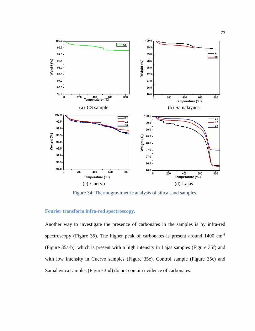
73

(a) CS sample (b) Samalayuca

(c) Cuervo (d) Lajas

Figure 34: Thermogravimetric analysis of silica sand samples.

Fourier transform infra-red spectroscopy.

Another way to investigate the presence of carbonates in the samples is by infra-red

spectroscopy (Figure 35). The higher peak of carbonates is present around 1400 cm-1

(Figure 35a-b), which is present with a high intensity in Lajas samples (Figure 35f) and

with low intensity in Cuervo samples (Figure 35e). Control sample (Figure 35c) and

Samalayuca samples (Figure 35d) do not contain evidence of carbonates.

74

(a) (b)

(c) (d)

(e) (f)

Figure 35: Infra-red spectra: (a) calcium carbonate, (b) sodium carbonate, (c) Control

sample, (d) Samalayuca samples, (e) Cuervo samples and (f) Lajas samples.

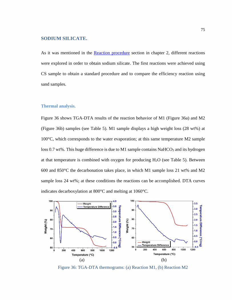
75

SODIUM SILICATE.

As it was mentioned in the Reaction procedure section in chapter 2, different reactions

were explored in order to obtain sodium silicate. The first reactions were achieved using

CS sample to obtain a standard procedure and to compare the efficiency reaction using

sand samples.

Thermal analysis.

Figure 36 shows TGA-DTA results of the reaction behavior of M1 (Figure 36a) and M2

(Figure 36b) samples (see Table 5). M1 sample displays a high weight loss (28 wt%) at

100°C, which corresponds to the water evaporation; at this same temperature M2 sample

loss 0.7 wt%. This huge difference is due to M1 sample contains NaHCO3 and its hydrogen

at that temperature is combined with oxygen for producing H2O (see Table 5). Between

600 and 850°C the decarbonation takes place, in which M1 sample loss 21 wt% and M2

sample loss 24 wt%; at these conditions the reactions can be accomplished. DTA curves

indicates decarboxylation at 800°C and melting at 1060°C.

(a) (b)

Figure 36: TGA-DTA thermograms: (a) Reaction M1, (b) Reaction M2

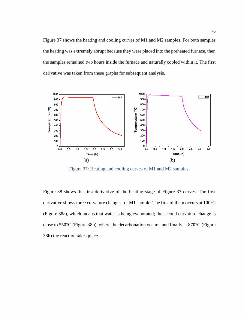
76

Figure 37 shows the heating and cooling curves of M1 and M2 samples. For both samples

the heating was extremely abrupt because they were placed into the preheated furnace, then

the samples remained two hours inside the furnace and naturally cooled within it. The first

derivative was taken from these graphs for subsequent analysis.

(a) (b)

Figure 37: Heating and cooling curves of M1 and M2 samples.

Figure 38 shows the first derivative of the heating stage of Figure 37 curves. The first

derivative shows three curvature changes for M1 sample. The first of them occurs at 100°C

(Figure 38a), which means that water is being evaporated; the second curvature change is

close to 550°C (Figure 38b), where the decarbonation occurs; and finally at 870°C (Figure

38b) the reaction takes place.

0.0 0.5 1.0 1.5 2.0 2.5 3.0 3.50

100

200

300

400

500

600

700

800

900

1000

Te

mp

era

ture

(°C

)

Time (h)

M1

0.0 0.5 1.0 1.5 2.0 2.5 3.0 3.50

100

200

300

400

500

600

700

800

900

1000

Te

mp

era

ture

(°C

)

Time (h)

M2

77

(a) (b)

(c) (d)

Figure 38: First derivative of sample heating.

M2 Sample shows a similar behavior to sample M1 while heating; however, it presents a

lower curvature change at 100°C (Figure 38c) and the decarbonation is more evident close

to 600°C; this information complements the DTA-TGA results. At 870°C (Figure 38d) the

last curvature change can be seen, which corresponds to the reaction.

A comparison between TGA-DTA and Furnace analyses is present in Table 11, where can

be seen that the results are consistent; therefore, sodium silicate can be obtained under these

conditions in other furnaces.

78

Table 11: Comparison between TGA-DTA and Furnace test.

Test type Sample Temperature

(°C)

Details

TGA-DTA

M1

100 Water evaporation

600 Decarbonation

850 Reaction

M2 600 Decarbonation

850 Reaction

Furnace

M1

100 Water evaporation

600 Decarbonation

870 Reaction

M2

100 Water evaporation

550 Decarbonation

870 Reaction

X-ray diffraction.

Figure 39 shows the X-ray diffraction pattern results of sodium silicate obtained by “M3-

solution” reaction by the chemical reactor process. As can be seen the efficiency reaction

is not what was expected because high peaks of silicon dioxide can be observed.

Although the presence of sodium silicate is evident, this is not the best procedure to produce

sodium silicate. Therefore, this reaction will no longer be studied.

Figure 39: X-ray diffraction of sodium silicate obtained by reaction “M3-solution”.

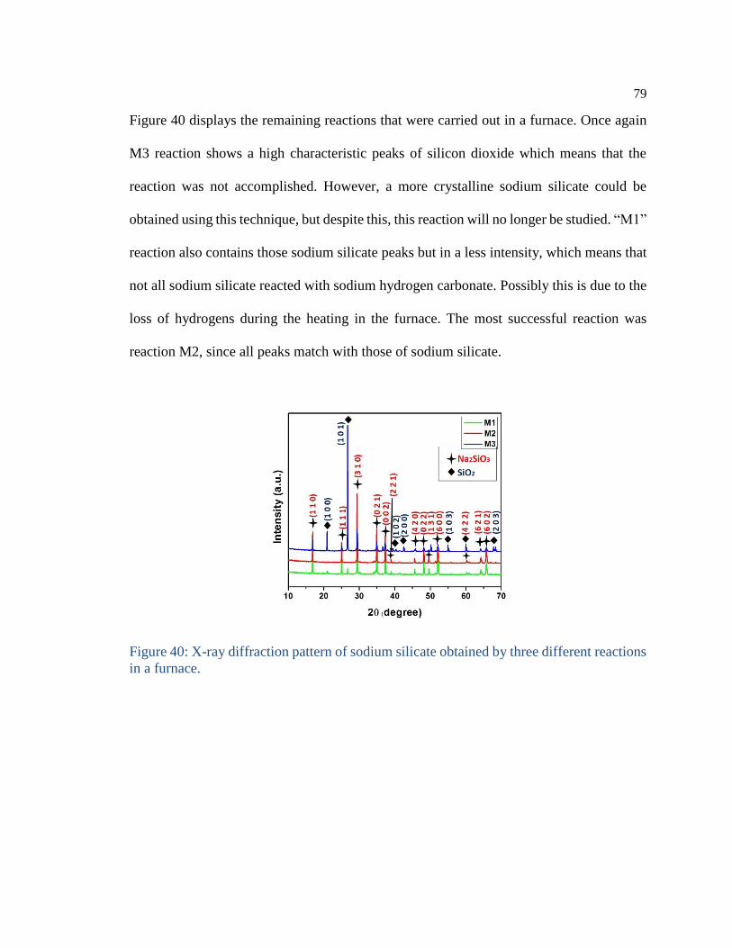
79

Figure 40 displays the remaining reactions that were carried out in a furnace. Once again

M3 reaction shows a high characteristic peaks of silicon dioxide which means that the

reaction was not accomplished. However, a more crystalline sodium silicate could be

obtained using this technique, but despite this, this reaction will no longer be studied. “M1”

reaction also contains those sodium silicate peaks but in a less intensity, which means that

not all sodium silicate reacted with sodium hydrogen carbonate. Possibly this is due to the

loss of hydrogens during the heating in the furnace. The most successful reaction was

reaction M2, since all peaks match with those of sodium silicate.

Figure 40: X-ray diffraction pattern of sodium silicate obtained by three different reactions

in a furnace.

80

Fourier transform infra-red spectroscopy.

Figure 41 shows the FTIR spectra of sodium silicate synthesized by the three different

routes. In order to compare the products (M1-M2), a commercial sodium silicate was

studied as a reference sample (Figure 41a). Once again M1 (Figure 41b) and M2 (Figure

41c) were the best reactions. Both samples show signs of carbonate, probably due to the

presence of CO2 generated during the cooling stage.

Table 12 displays the assignments of IR and Raman vibrations according to Halasz et al

[42] and Gunasekaran et al [43].

(a)

Figure 41: Infra-red spectra of sodium silicates, (a) commercial sample, (b) sample M1,

and (c) sample M2 (continued on next page).

81

(b) (c)

Figure 41: Infra-red spectra of sodium silicates: (a) commercial sample, (b) sample M1,

and (c) sample M2 (continued from previous page).

Table 12: Assignments of IR and Raman vibrations of solid, crystalline sodium metasilicate

[42, 43].

Frequencies (cm-1)

Assignments IR Raman

1034 - vas Si-O(Na) “possible”

1435 - v3 Asymmetric CO3 stretching

968 972 vas Si-O(Si)

897 - vs Si-O(Na)

876 v2-Asymmetric CO3 deformation

- 756 δas (H)O-Si-O(H)

712 - v4-Asymmetric CO3 deformation

713 - vs Si-O(Si)

592 592 δas as (Na)O-Si-O(Na)

525 - δas (Si)O-Si-O(Si)

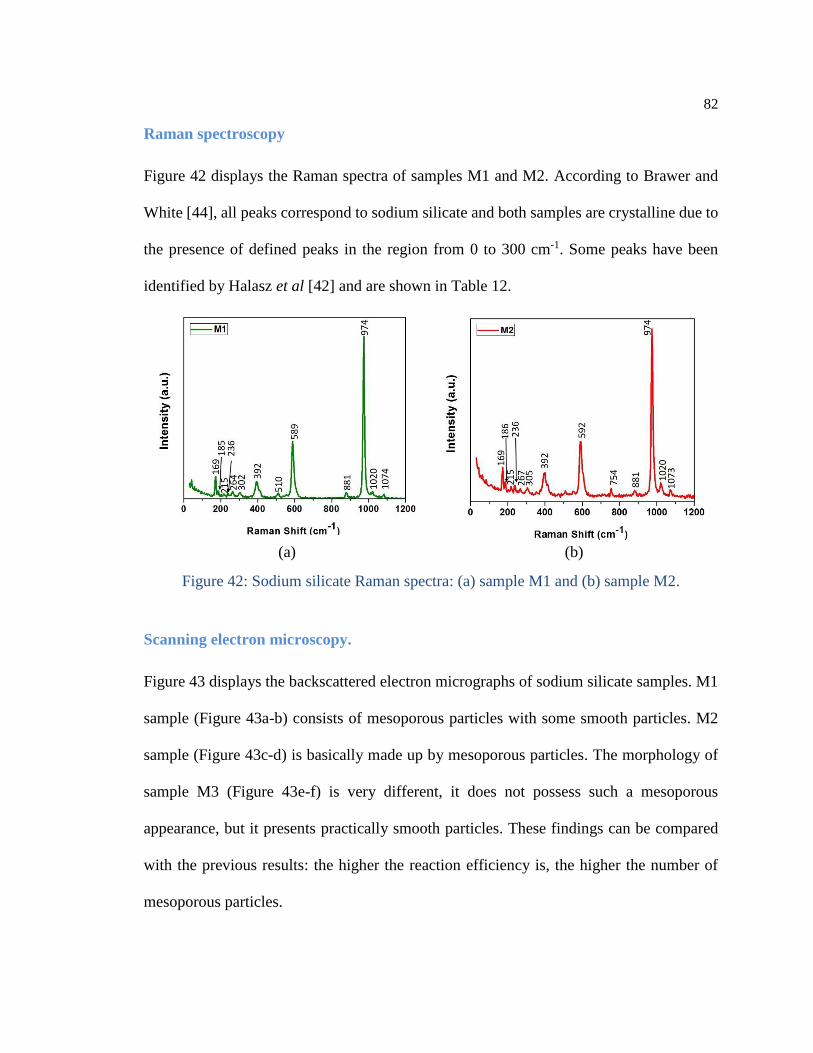
82

Raman spectroscopy

Figure 42 displays the Raman spectra of samples M1 and M2. According to Brawer and

White [44], all peaks correspond to sodium silicate and both samples are crystalline due to

the presence of defined peaks in the region from 0 to 300 cm-1. Some peaks have been

identified by Halasz et al [42] and are shown in Table 12.

(a) (b)

Figure 42: Sodium silicate Raman spectra: (a) sample M1 and (b) sample M2.

Scanning electron microscopy.

Figure 43 displays the backscattered electron micrographs of sodium silicate samples. M1

sample (Figure 43a-b) consists of mesoporous particles with some smooth particles. M2

sample (Figure 43c-d) is basically made up by mesoporous particles. The morphology of

sample M3 (Figure 43e-f) is very different, it does not possess such a mesoporous

appearance, but it presents practically smooth particles. These findings can be compared

with the previous results: the higher the reaction efficiency is, the higher the number of

mesoporous particles.

83

EDS analyses (Table 13) were performed on the whole sample surface to verify that the

most important elements of sodium silicate are present in the samples; as can be seen, there

are some similitudes in the three samples. The EDS results cannot say how efficient was

the reaction, but they give an idea of the relation of the sodium silicate elements.

Table 13: Energy dispersive spectroscopy (EDS) results of sodium silicates (wt%).

Sample O Na Si Fe

M1 40.6 ± 0.1 35.2 ± 0.1 20.8 ± 0.1 0.7 ± 0.1

M2 39.1 ± 0.2 36.2 ± 0.1 23.6 ± 0.1 0.5 ± 0.1

M3 44.2 ± 0.2 31.5 ± 0.2 23.9 ± 0.1 0.4 ± 0.1

(a) (b)

Figure 43: Backscattered electron micrographs of sodium silicate samples: (a) and (b) M1

sample, (c) and (d) M2 sample and (e) and (f) M3 sample, (continued on next page).

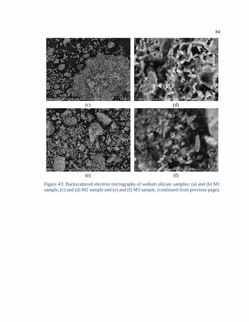
84

(c) (d)

(e) (f)

Figure 43: Backscattered electron micrographs of sodium silicate samples: (a) and (b) M1

sample, (c) and (d) M2 sample and (e) and (f) M3 sample, (continued from previous page).

85

CHAPTER 4: CONCLUSIONS AND FUTURE WORK

Conclusions.

- All different silica sand banks analyzed were similar in aspect, size and

morphology, except lajas sand banks whose size were bigger.

- The main phase of silica sand banks was silicon dioxide in a medium to high

concentration. The most suitable silica sand banks were, in this order, Samalayuca

2 and 1.

- Lajas silica sand banks have a higher content of carbonates, which could cause an

incomplete reaction.

- Thermal analysis indicates that the reaction takes place at approximately 870°C to

produce a granular sodium silicate. After 1060°C a sodium metasilicate can be

obtained, but the application of a thermal shock is necessary to separate the product

of the crucible.

- TGA-DTA revealed that reaction M1 lost a high percentage of weight during its

heating due to the presence of hydrogen (from the acid sodium carbonate), which

combined with oxygen produced high amount of water. This weight loss causes

that the reaction cannot be finished at all and that by XRD reflections of silicon

dioxide have been seen; furthermore, mesoporous particles were observed by SEM.

86

- A poor sodium silicate could be synthesized using soda as a reactant (reaction M3).

This reaction was performed in two ways, the most effective was that carried out in

the furnace. However, X-ray diffraction patterns revealed high peaks of silicon

dioxide and SEM micrographs showed absence of mesoporous particles.

- The best route to produce sodium silicate is by reacting sodium carbonate with

silicon dioxide in stoichiometric concentrations (reaction M2). The adequate

temperature to accomplish the synthesis is between 870°C and 1000°C. The

efficiency of the reaction was demonstrated by XRD, SEM and Raman

Spectroscopy.

87

Future work.

- Synthesize sodium silicate from Samalayuca silica sand using reaction M2 and

characterize it.

- Produce in a pilot plant sodium silicate from this silica sand bank and use it to

obtain a geopolymer.

- Evaluate the mechanical properties of geopolymer as they are:

o Compressive test,

o Drying shrinkage,

o Expansion in autoclave,

o Expansion in water and,

o Curing time.

- Compare its mechanical properties with a Portland cement.

88

REFERENCES

[1] Donaldson, Erle C. Alam, waqi, "Chemistry of silica sand," in Wettability, Gulf

Publishing Company, 2008, pp. 223-226.

[2] E. G. Rochow, "The Chemistry of Silicon," in Pergamon Texts in Inorganic

Chemistry, vol. 9, New York, Pergamon Press, 1973, pp. 1323-1465.

[3] B. Eduardo, Mineralogía de arcillas de suelos, Costa Rica: CIDIA, 1985.

[4] C. Klein, Manual de Mineralogía, vol. 4, Barcelona: Reverté, 2003.

[5] John R. Brown,Foseco (F.S.) Limited, The Foseco Foundryman's Handbook, vol.

10th edition, Oxford: Pergamon Press, 1994.

[6] S. M. Bulatovic, Handbook of Flotation Reagents, Oxford: Elsevier, 2007, p. 65.

[7] G. Schimmel, "Process for the preparation of crystalline sodium silicates". United

States Patent 5183651, 2 February 1993.

[8] B. E. V. Rehren, "Silicatos cristalinos de sodio/potasio". México Patent 198108, 16

August 2000.

[9] J. Deabriges, "Process for the manufacture of sodium silicate". United States Patent

4336235, 22 June 1982.

[10] J. Deabriges, "Método mejorado para la producción de silicato de sodio". México

Patent 006875, 11 September 1986.

[11] G. Schimmel, "Process for producing amorphous sodium silicate". United States

Patent 5229095, 20 July 1993.

[12] Norma Mexicana NMX-K-240-SCFI-2009, Silicato de sodio o potasio para uso

industrial, Mexico, D.F..

[13] Jessica Elzea Kogel, Nikhil C. Trivedi, James M. Barker Stanley T. Krukowski,

Industrial Minerals and Rocks, 7TH ed., Littleton, Colorado: Society for Mining,

Metallurgy, and Exploration, Inc., 2006.

[14] B. Singh, G. Ishwarya, M. Gupta, S.K. Bhattacharyya, "Geopolymer concrete: A

review of some recent developments," Construction and Building Materials,, vol. 85,

pp. 78-90, 2015.

89

[15] Troitzsch, Jurgen, Plastics Flammability Handbook, vol. 3, D. J. Troitzsch, Ed.,

Munich: Hanser, 2004.

[16] J. Provis, Geopolymers-Structure, Processing, Properties and Industrial Applications,

Australi: Woodhead Publishing, 2009.

[17] Benjamin C. McLellan and others, "Costs and carbon emissions for geopolymer

pastes in comparison to ordinary portland cement," Journal of Cleaner Production,

vol. 19, pp. 1080-1090, 2011.

[18] B. D. Cullity, Elements of X-ray diffraction, Massachusets: Addison-Wesley

Publishing , 1956.

[19] B. L. Dutrow, C. M. Clark., "Serc. Carleton," Montanta State University, 2015.

[Online]. Available:

http://serc.carleton.edu/research_education/geochemsheets/techniques/XRD.html.

[20] A. Guinier, X-ray diffraction, in crystals, imperfect crystals and amprphous bodies,

Ontario: General Publishing Company, 1994.

[21] C. Suryanarayana and M. Grant Norton, X-ray diffraction, A practical approach, New

York: Plenum Publishing Corporation, 1998.

[22] C. Hammond, The basics of crystallography and diffraction, 4 ed., Oxford: Oxford

Science Publications, 2015.

[23] K. R. Pring and MW. Davidson, "Olympusmicro," OLYMPUS America Inc., 2012.

[Online]. Available:

http://www.olympusmicro.com/primer/anatomy/components.html.

[24] Goldstein J.I., L.C.E., Newbury D.E., Lifshin E., Echlin P., Sawyer L., Joy D.C.,

Michael J.R., Scanning Electron Microscopy and X-Ray Microanalysis, 3 ed., New

York: Plenum Publishers, 1992.

[25] D. Mogk, "Serc. Carleton," Montana State University, 2015. [Online]. Available:

http://serc.carleton.edu/research_education/geochemsheets/techniques/SEM.html.

[26] J. Schweitzer., "Radiological and environmental Management," Purdue University,

2010. [Online]. Available: https://www.purdue.edu/ehps/rem/rs/sem.htm.

[27] Attberry, "How stuff works," 2013. [Online]. Available:

http://science.howstuffworks.com/scanning-electron-microscope2.htm.

90

[28] University of California Riverside, "Central Facility for Advanced Microscopy and

Microanalysis," 2014. [Online]. Available:

http://micron.ucr.edu/public/manuals/Sem-intro.pdf. [Accessed 2014].

[29] J. Börgesson., "Physics and Engineering Pysics," Goteborg University, 2009.

[Online]. Available:

http://www.fy.chalmers.se/microscopy/students/imagecourse/SEMlabPM.pdf.

[30] R. F. Speyer, Thermal analyisis of materials, New York: Marcel Dekker, 1994.

[31] M. E. Brown, Handbook of the thermal analysis and calorimetry, Amsterdam:

Elsevier, 1998.

[32] Perkin Elmer, "Perkin Elmer Inc.," 2010. [Online]. Available:

http://www.perkinelmer.com/CMSResources/Images/44-

74556GDE_TGABeginnersGuide.pdf.

[33] American Society for Testing and Materials, The theory and properties of

thermocouple elements, Baltimore, 1971.

[34] American Society for Testing and Materials, Manual on the use of thermocouples in

temperature measurement, 1974.

[35] Thermoscientific, Thermo Fisher Scientific Inc., 2015. [Online]. Available:

http://www.thermoscientific.com/en/products/fourier-transform-infrared-

spectroscopy-ftir.html.

[36] C. A. Rice, "Jet-FTIR Spectroscopy of Biomolecular Model Systems," Cuvillier

Verlag Göttingen, Göttingen, Germany, 2007.

[37] Centre for materials Education, "doitpoms," University of Cambridge UK , 2004.

[Online]. Available: http://www.doitpoms.ac.uk/tlplib/raman/active_modes.php.

[38] Ferraro, J.R., K. Nakamoto, and C. W. Brown, Introductory Raman Spectroscopy,

2nd ed., ELSEVIER, 2003.

[39] C. Rathmell, "Ocean Optics," Ocean Optics, Inc., 1989-2015. [Online]. Available:

http://oceanoptics.com/measurementtechnique/raman/.

[40] S. J. Dick, Rubber Technology - Compounding and Testing for Performance, second

ed., Hanser, 2009.

[41] E. Scientifiques, "ES-France," 2012. [Online]. Available: http://www.es-

france.com/pdf/1180_us_doctech.pdf.

91

[42] Istvan Halasz, Mukesh Agarwal, Runbo Li, and Neil Miller, "Vibrational spectra and

dissociation of aqueous Na2SiO3 solutions," Springer Science, vol. 117, 2007.

[43] S. Gunasekaran, G. Anbalagan and S. Pandi, "Raman and infrared spectra of

carbonates of calcite structure," Journal of Raman Spectroscopy, vol. 36, pp. 892-

899, 2006.

[44] Steven A. Brawer and William B. White, "Raman spectroscopic investigation of the

structure of silicate glasses. I. The binary alkali silicates," Chemical and Physics, vol.

63, p. 2421, 1975.