bonta desarrollo jy utilidad de la curva de huff

7/27/2019 Bonta Desarrollo Jy Utilidad de La Curva de Huff

http://slidepdf.com/reader/full/bonta-desarrollo-jy-utilidad-de-la-curva-de-huff 1/13

Applied Engineering in Agriculture

Vol. 20(5): 641−653 2004 American Society of Agricultural Engineers ISSN 0883−8542 641

DEVELOPMENT AND UTILITY OF HUFF CURVES FOR

DISAGGREGATING PRECIPITATION AMOUNTS

J. V. Bonta

ABSTRACT. Watershed models are becoming more sophisticated and require temporal inputs of precipitation to drive themodeled hydrologic processes. Short time increments of the order of minutes are particularly needed, but these are seldomavailable or do not have good spatial coverage. The most widely available precipitation data in the United States are totalamounts for 24−h periods. Information on the actual intensity distribution within a period of precipitation is lacking and practitioners resort to approximate methods to distribute the precipitation in time (“disaggregation”). The most commonapproach to disaggregate total precipitation amounts has been to use “design storms,” fixed patterns of the time distributionof precipitation intensities within a period. “ Huff curves” provide a method of characterizing storm mass curves. They area probabilistic representation of accumulated storm depths for corresponding accumulated storm durations expressed indimensionless form. The development of Huff curves is described in the present study using precipitation data from Coshocton,Ohio because the procedure has never been documented in the literature. The potential use of these curves, the state of knowledge, and research needs for advancing the utility of Huff curves for storm disaggregation are summarized. Threeapproaches for using Huff curves to disaggregate precipitation totals are described: design storms (fixed patterns of intensities), stochastic simulation of within−storm intensities, and a hybrid of these two approaches. Expanded use of Huff

curves as described in the latter two approaches offer opportunities for maximizing the information contained in Huff curves.There is no meaningful correspondence between NRCS design storms (Types I, IA, II, and III) and Huff curves. A computer program is available to facilitate the development of Huff curves for stimulating research into their practical use.

Keywords. Huff curves, Storm simulation, Storm synthesis, Stochastic simulation, Design storm, Disaggregation, precipitation.

atershed models are required for many pur-poses such as engineering design for runoff and erosion control in agricultural and urbanareas, water−quality evaluations, global−

change investigations, etc. Precipitation inputs to models areoften in the form of either measured precipitation or “design

storms” (fixed patterns of the time distribution of precipita-tion intensities, often referred to as “storm profiles”). Designstorms are often used for engineering design for storm−watercontrol (e.g., urban areas) because time distributions of pre-cipitation for time intervals less than a day are needed but areoften not available. Design storms “disaggregate” total pre-cipitation to synthesize within−storm intensities. They are as-sumed to be representative of the general trend of thevariation of precipitation intensities, but they are inadequatefor this purpose because an “expected” time distribution nev-er occurs. This is because observed precipitation within astorm has both random and deterministic components, result-ing in an infinite number of possible time distributions of in-tensities within a storm.

The most widely used precipitation inputs to watershedmodels are total amounts for 24−h periods. This is because of

Article was submitted for review in December 2003; approved forpublication by the Soil & Water Division of ASAE in April 2004.

The author is James V. Bonta, ASAE Member Engineer, ResearchHydraulic Engineer, USDA−Agricultural Research Service, North

Appalachian Experimental Watershed, Coshocton, Ohio 43812; phone:740−545−6349 fax: 740−545−5125 e−mail:[email protected].

the large geographic coverage and long records of these data.However, information on the actual intensity distributionwithin the 24−h period is lacking and practitioners resort todesign storms to distribute subdaily precipitation. Hourlyprecipitation data are available to a lesser aerial extent overthe United States, which can be directly used for inputs to

models. Additionally, these data are useful for developingmethods for distributing intensities. Fifteen−minute precipi-tation is available, but to even a lesser aerial extent thanhourly data. Another source of available precipitation data isintensity−duration−frequency (IDF) precipitation data. How-ever, these uniform intensities are developed only frommaximum intensities within storms, and thus representincomplete storms. Incomplete storms do not includeintensities prior to the maximum precipitation burst thatsatisfies a soil−water deficit incorporated into many wa-tershed models.

Another source of precipitation “data” to watershedmodels is from weather−generation models (e.g., CLIGEN,Nicks et al., 1995; GEM, Hanson et al., 1989, 1994, and

2002). These models can simulate temporally distributedestimates of precipitation amounts and other weather ele-ments by using known statistical characteristics of weather(”stochastic simulation”). However, the smallest time−stepthat is currently generated is often only 24 h because of thewidespread availability of these data used to parameterizethese models. Consequently, precipitation intensities must beartificially distributed in time given only the 24−h totalamounts. CLIGEN includes an undocumented breakpointprecipitation simulator (Zeleke et al., 2000). The An-nAGNPS watershed model (Bingner and Theurer, 2001) uses

W

DESARROLLO Y UTILIDAD DE LA CURVA DE HUFF PARA

DESAGREGAR LA CANTIDAD DE LA PRECIPITACION



642 APPLIED ENGINEERING IN AGRICULTURE

the various Natural Resources Conservation Service (NRCS)“Type” profiles to distribute 24−h totals over spatiallydistributed landscape cells (Theurer, F., 2003, personalcommunication). Algorithms for stochastic storm simulationof short−time increment precipitation data are largelyunderdeveloped.

Perhaps the most common design storms used in practiceare the various distributions of the NRCS (i.e., Types I, IA,II, and III; SCS, 1986). Other patterns have been developedand many are used today such as, Kiefer and Chu (1957), Yen

and Chow (1980), Desbordes and Raous (1976), Sifalda(1973), Pilgrim and Cordery (1975), Pilgrim et al. (1969),Natural Environment Research Council (NERC, 1975),Sutherland (1982), Asquith et al. (2003), Huff (1967; 1990),Huff and Angel (1989; 1992).

An assumption often made for estimating the magnitudeof peak runoff rates is that the frequencies of occurrence of the peak flow and causal precipitation are the same. Pilgrimand Cordery (1975) suggest that this is true if median oraverage values of parameters are used, but this assumption isunproven. It is also assumed that the season of largestprecipitation intensities cause the largest peak flow rates.This assumption is not necessarily the case in smallagricultural watersheds (Bonta and Rao, 1994), but may be

for urban areas where antecedent soil−water deficit is not amajor factor. Problems with the design−storm concept andsuggestions for improving rainfall inputs to urban watershedmodels are discussed in Patry and McPherson (1979).

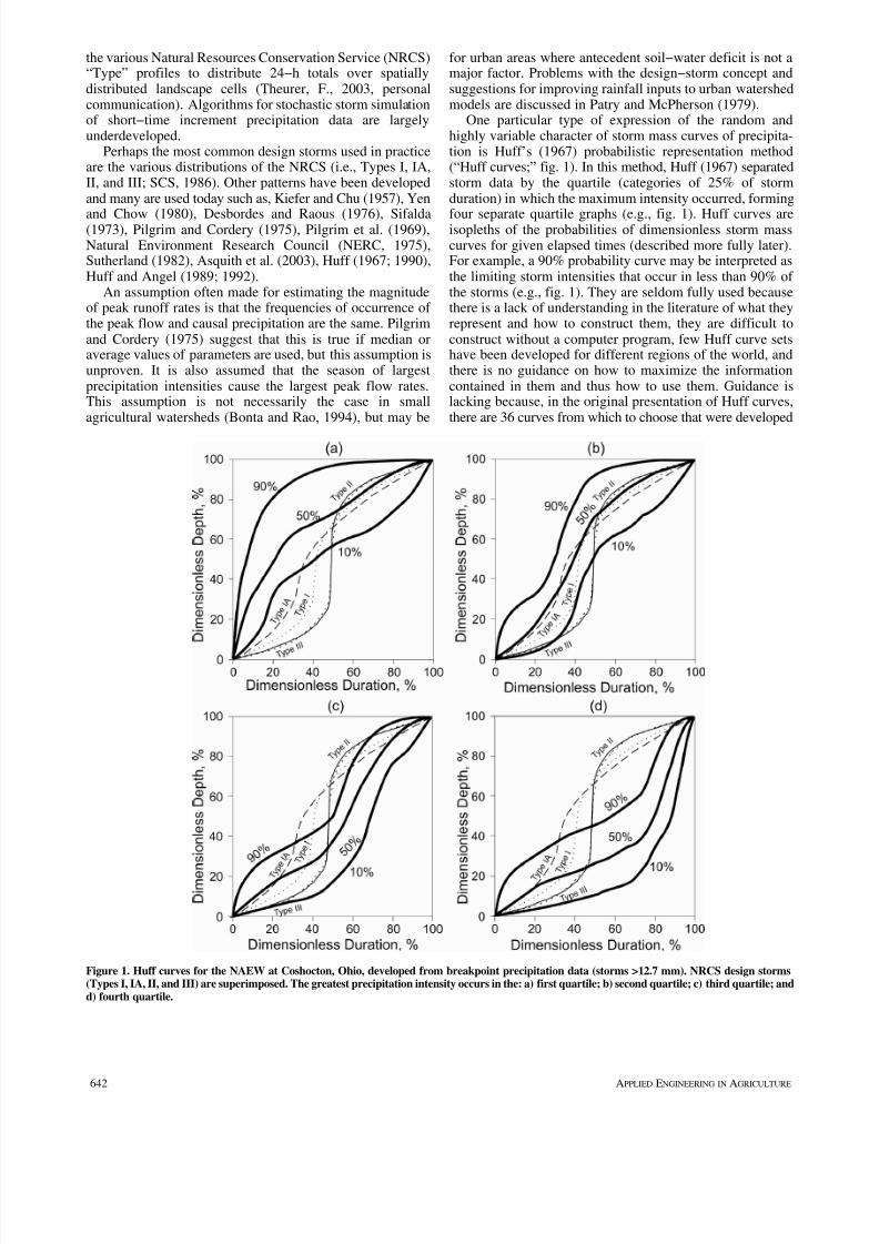
One particular type of expression of the random andhighly variable character of storm mass curves of precipita-tion is Huff’s (1967) probabilistic representation method(“Huff curves;” fig. 1). In this method, Huff (1967) separatedstorm data by the quartile (categories of 25% of stormduration) in which the maximum intensity occurred, forming

four separate quartile graphs (e.g., fig. 1). Huff curves areisopleths of the probabilities of dimensionless storm masscurves for given elapsed times (described more fully later).For example, a 90% probability curve may be interpreted asthe limiting storm intensities that occur in less than 90% of the storms (e.g., fig. 1). They are seldom fully used becausethere is a lack of understanding in the literature of what theyrepresent and how to construct them, they are difficult toconstruct without a computer program, few Huff curve setshave been developed for different regions of the world, andthere is no guidance on how to maximize the informationcontained in them and thus how to use them. Guidance islacking because, in the original presentation of Huff curves,there are 36 curves from which to choose that were developed

Figure 1. Huff curves for the NAEW at Coshocton, Ohio, developed from breakpoint precipitation data (storms >12.7 mm). NRCS design storms(Types I, IA, II, and III) are superimposed. The greatest precipitation intensity occurs in the: a) first quartile; b) second quartile; c) third quartile; andd) fourth quartile.



643Vol. 20(5): 641−653

using Illinois precipitation data (Huff, 1967), and criteria forselecting a curve for use in any region of the United States arelacking. Three approaches to temporally disaggregate storm,24−h, and other precipitation totals using Huff curves havebeen investigated in recent years and are the subject of thepresent article: design storms, stochastic generation of stormintensities, and a hybrid of these two approaches.

OBJECTIVES

Information contained in Huff curves is seldom fully

utilized but these curves offer opportunities for practical usefor disaggregating precipitation totals. Detail on constructionof Huff curves is not documented in the literature, and theiruse has been limited for the reasons mentioned earlier. Also,areas for further study can be identified based on presentknowledge and use of Huff curves. The objectives of thisarticle are to: 1) present the conceptual and mathematicaldevelopment of Huff curves; 2) describe applications andapproaches for use of Huff curves for design storms,stochastic simulation, and a hybrid approach; 3) summarizeinformation on the effects of factors affecting the curves; and4) discuss research needs. A computer program is availableto readers for developing Huff curves to facilitate morewidespread use, and is also briefly described. This article is

intended to summarize what is known about Huff curves andto stimulate thinking on how to extract the maximum amountof information contained in Huff curves for practical use inprecipitation and watershed modeling.

PROCEDURE

DATA USED FOR THE PRESENT STUDY

Data from rain gage RG100 on the USDA – AgriculturalResearch Service facility at the North Appalachian Experi-mental Watershed (NAEW) located near Coshocton, Ohio,are used to describe the procedure for developing Huff curvesand for evaluating some features of Huff curves. Data fromRG109 and RG115 are also used for some purposes. Thesethree gages are located about 1.5 km from each other on the425−ha NAEW facility. Data from these gages are tabulatedat changes in precipitation intensity (“breakpoint” data) forthe period of record from 1937 through 1994. Data fromRG119 are also used for regional comparisons. Some featuresof Huff’s original development are modified as explained inthe steps that follow. Average annual precipitation is about948 mm for the NAEW at Coshocton, Ohio.

DATA USED BY HUFF

In his original work, Huff (1967) used 12 years of datafrom 49 gages over an area of 1037 km2in eastern Illinois.The gaged area was topographically a flat prairie with

elevations ranging from 198 to 277 m. He used storm datagreater than a rain−gage network mean of 12.7 mm and/orwhen one or more gages recorded more than 25.4 mm. Stormdurations used ranged from 1 to 48 hours. The study by Huff (1990) updated the previous study by including an additional12 gages in a 25.9−km2 Champaign−Urbana, Illinois area,and 6 more gages in the Chicago area (Huff and Vogel, 1976)to include 417 more storms. The latest work on Huff curvesin Illinois is by Huff and Angel (1992) in which they used thecurves from Huff (1990). Their Huff−curve−related results

are developed strictly from east−central Illinois and are notbased on data collected over an extensive area.

STORM IDENTIFICATION

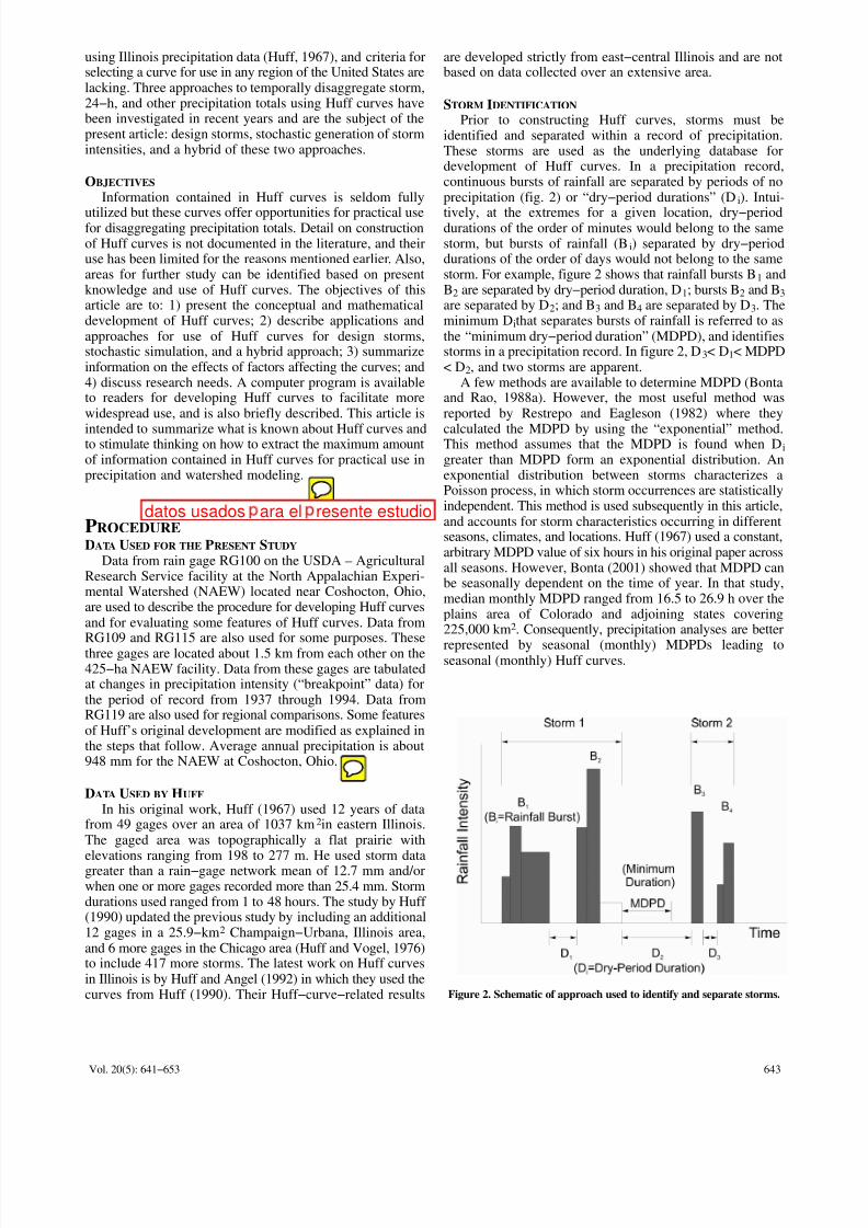
Prior to constructing Huff curves, storms must beidentified and separated within a record of precipitation.These storms are used as the underlying database fordevelopment of Huff curves. In a precipitation record,continuous bursts of rainfall are separated by periods of noprecipitation (fig. 2) or “dry−period durations” (Di). Intui-

tively, at the extremes for a given location, dry−perioddurations of the order of minutes would belong to the samestorm, but bursts of rainfall (Bi) separated by dry−perioddurations of the order of days would not belong to the samestorm. For example, figure 2 shows that rainfall bursts B1 andB2 are separated by dry−period duration, D1; bursts B2 and B3

are separated by D2; and B3 and B4 are separated by D3. Theminimum Dithat separates bursts of rainfall is referred to asthe “minimum dry−period duration” (MDPD), and identifiesstorms in a precipitation record. In figure 2, D3< D1< MDPD< D2, and two storms are apparent.

A few methods are available to determine MDPD (Bontaand Rao, 1988a). However, the most useful method wasreported by Restrepo and Eagleson (1982) where they

calculated the MDPD by using the “exponential” method.This method assumes that the MDPD is found when Di

greater than MDPD form an exponential distribution. Anexponential distribution between storms characterizes aPoisson process, in which storm occurrences are statisticallyindependent. This method is used subsequently in this article,and accounts for storm characteristics occurring in differentseasons, climates, and locations. Huff (1967) used a constant,arbitrary MDPD value of six hours in his original paper acrossall seasons. However, Bonta (2001) showed that MDPD canbe seasonally dependent on the time of year. In that study,median monthly MDPD ranged from 16.5 to 26.9 h over theplains area of Colorado and adjoining states covering225,000 km2. Consequently, precipitation analyses are better

represented by seasonal (monthly) MDPDs leading toseasonal (monthly) Huff curves.

Figure 2. Schematic of approach used to identify and separate storms.

datos usados ara el resente estudio




DEVELOPMENT OF HUFF CURVES FROM MEASURED DATA

CURVES FROM COSHOCTON POINT RAIN−GAGE DATA

There are two types of Huff curves: point−developed andarea−averaged. This section assumes curves are developedfrom data from an individual rain gage (“point”). Area−aver-aged curves are discussed in the next section, but theprocedure is identical to point−developed curves after anintermediate step.

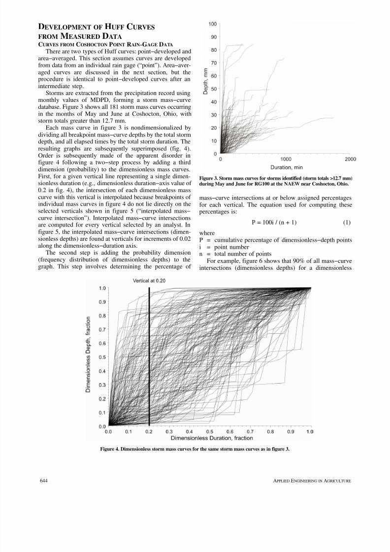
Storms are extracted from the precipitation record usingmonthly values of MDPD, forming a storm mass−curvedatabase. Figure 3 shows all 181 storm mass curves occurringin the months of May and June at Coshocton, Ohio, withstorm totals greater than 12.7 mm.

Each mass curve in figure 3 is nondimensionalized bydividing all breakpoint mass−curve depths by the total stormdepth, and all elapsed times by the total storm duration. Theresulting graphs are subsequently superimposed (fig. 4).Order is subsequently made of the apparent disorder infigure 4 following a two−step process by adding a thirddimension (probability) to the dimensionless mass curves.First, for a given vertical line representing a single dimen-sionless duration (e.g., dimensionless duration−axis value of

0.2 in fig. 4), the intersection of each dimensionless masscurve with this vertical is interpolated because breakpoints of individual mass curves in figure 4 do not lie directly on theselected verticals shown in figure 5 (“interpolated mass−curve intersection”). Interpolated mass−curve intersectionsare computed for every vertical selected by an analyst. Infigure 5, the interpolated mass−curve intersections (dimen-sionless depths) are found at verticals for increments of 0.02along the dimensionless−duration axis.

The second step is adding the probability dimension(frequency distribution of dimensionless depths) to thegraph. This step involves determining the percentage of

Figure 3. Storm mass curves for storms identified (storm totals >12.7 mm)during May and June for RG100 at the NAEW near Coshocton, Ohio.

mass−curve intersections at or below assigned percentagesfor each vertical. The equation used for computing thesepercentages is:

P = 100i / (n + 1) (1)

whereP = cumulative percentage of dimensionless−depth pointsi = point numbern = total number of points

For example, figure 6 shows that 90% of all mass−curveintersections (dimensionless depths) for a dimensionless

Figure 4. Dimensionless storm mass curves for the same storm mass curves as in figure 3.



645Vol. 20(5): 641−653

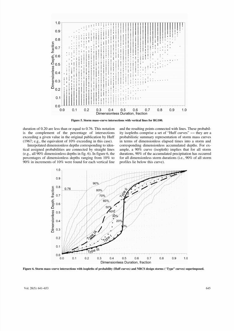
Figure 5. Storm mass−curve intersections with vertical lines for RG100.

duration of 0.20 are less than or equal to 0.76. This notationis the complement of the percentage of intersectionsexceeding a given value in the original publication by Huff (1967; e.g., the equivalent of 10% exceeding in this case).

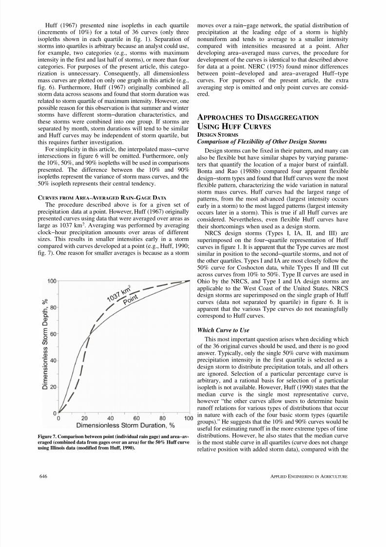
Interpolated dimensionless depths corresponding to iden-tical assigned probabilities are connected by straight lines(e.g., all 90% dimensionless depths in fig. 6). In figure 6, thepercentages of dimensionless depths ranging from 10% to90% in increments of 10% were found for each vertical line

and the resulting points connected with lines. These probabil-ity isopleths comprise a set of “Huff curves” −− they are aprobabilistic summary representation of storm mass curvesin terms of dimensionless elapsed times into a storm andcorresponding dimensionless accumulated depths. For ex-ample, a 90% curve (isopleth) implies that for all stormdurations, 90% of the accumulated precipitation has occurredfor all dimensionless storm durations (i.e., 90% of all stormprofiles lie below this curve).

Figure 6. Storm mass−curve intersections with isopleths of probability (Huff curves) and NRCS design storms (“Type” curves) superimposed.




Huff (1967) presented nine isopleths in each quartile(increments of 10%) for a total of 36 curves (only threeisopleths shown in each quartile in fig. 1). Separation of storms into quartiles is arbitrary because an analyst could use,for example, two categories (e.g., storms with maximumintensity in the first and last half of storms), or more than fourcategories. For purposes of the present article, this catego-rization is unnecessary. Consequently, all dimensionlessmass curves are plotted on only one graph in this article (e.g.,fig. 6). Furthermore, Huff (1967) originally combined all

storm data across seasons and found that storm duration wasrelated to storm quartile of maximum intensity. However, onepossible reason for this observation is that summer and winterstorms have different storm−duration characteristics, andthese storms were combined into one group. If storms areseparated by month, storm durations will tend to be similarand Huff curves may be independent of storm quartile, butthis requires further investigation.

For simplicity in this article, the interpolated mass−curveintersections in figure 6 will be omitted. Furthermore, onlythe 10%, 50%, and 90% isopleths will be used in comparisonspresented. The difference between the 10% and 90%isopleths represent the variance of storm mass curves, and the50% isopleth represents their central tendency.

CURVES FROM AREA−AVERAGED RAIN−GAGE DATA

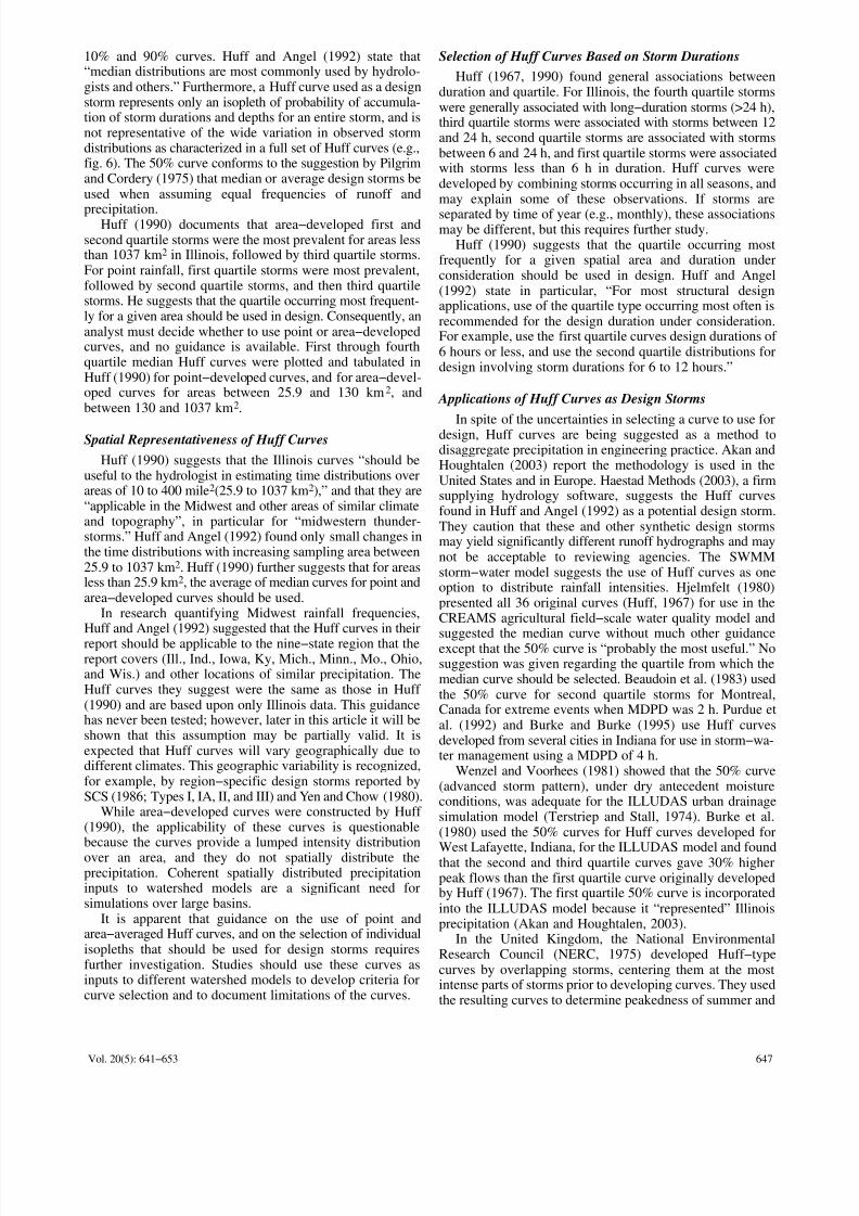
The procedure described above is for a given set of precipitation data at a point. However, Huff (1967) originallypresented curves using data that were averaged over areas aslarge as 1037 km2. Averaging was performed by averagingclock−hour precipitation amounts over areas of differentsizes. This results in smaller intensities early in a stormcompared with curves developed at a point (e.g., Huff, 1990;fig. 7). One reason for smaller averages is because as a storm

Figure 7. Comparison between point (individual rain gage) and area−av-eraged (combined data from gages over an area) for the 50% Huff curveusing Illinois data (modified from Huff, 1990).

moves over a rain−gage network, the spatial distribution of precipitation at the leading edge of a storm is highlynonuniform and tends to average to a smaller intensitycompared with intensities measured at a point. Afterdeveloping area−averaged mass curves, the procedure fordevelopment of the curves is identical to that described abovefor data at a point. NERC (1975) found minor differencesbetween point−developed and area−averaged Huff−typecurves. For purposes of the present article, the extraaveraging step is omitted and only point curves are consid-

ered.

APPROACHES TO DISAGGREGATION USING HUFF CURVES

DESIGN STORMS

Comparison of Flexibility of Other Design Storms

Design storms can be fixed in their pattern, and many canalso be flexible but have similar shapes by varying parame-ters that quantify the location of a major burst of rainfall.Bonta and Rao (1988b) compared four apparent flexibledesign−storm types and found that Huff curves were the mostflexible pattern, characterizing the wide variation in natural

storm mass curves. Huff curves had the largest range of patterns, from the most advanced (largest intensity occursearly in a storm) to the most lagged patterns (largest intensityoccurs later in a storm). This is true if all Huff curves areconsidered. Nevertheless, even flexible Huff curves havetheir shortcomings when used as a design storm.

NRCS design storms (Types I, IA, II, and III) aresuperimposed on the four−quartile representation of Huff curves in figure 1. It is apparent that the Type curves are mostsimilar in position to the second−quartile storms, and not of the other quartiles. Types I and IA are most closely follow the50% curve for Coshocton data, while Types II and III cutacross curves from 10% to 50%. Type II curves are used inOhio by the NRCS, and Type I and IA design storms are

applicable to the West Coast of the United States. NRCSdesign storms are superimposed on the single graph of Huff curves (data not separated by quartile) in figure 6. It isapparent that the various Type curves do not meaningfullycorrespond to Huff curves.

Which Curve to Use

This most important question arises when deciding whichof the 36 original curves should be used, and there is no goodanswer. Typically, only the single 50% curve with maximumprecipitation intensity in the first quartile is selected as adesign storm to distribute precipitation totals, and all othersare ignored. Selection of a particular percentage curve is

arbitrary, and a rational basis for selection of a particularisopleth is not available. However, Huff (1990) states that themedian curve is the single most representative curve,however “the other curves allow users to determine basinrunoff relations for various types of distributions that occurin nature with each of the four basic storm types (quartilegroups).” He suggests that the 10% and 90% curves would beuseful for estimating runoff in the more extreme types of timedistributions. However, he also states that the median curveis the most stable curve in all quartiles (curve does not changerelative position with added storm data), compared with the



647Vol. 20(5): 641−653

10% and 90% curves. Huff and Angel (1992) state that“median distributions are most commonly used by hydrolo-gists and others.” Furthermore, a Huff curve used as a designstorm represents only an isopleth of probability of accumula-tion of storm durations and depths for an entire storm, and isnot representative of the wide variation in observed stormdistributions as characterized in a full set of Huff curves (e.g.,fig. 6). The 50% curve conforms to the suggestion by Pilgrimand Cordery (1975) that median or average design storms beused when assuming equal frequencies of runoff and

precipitation.Huff (1990) documents that area−developed first andsecond quartile storms were the most prevalent for areas lessthan 1037 km2 in Illinois, followed by third quartile storms.For point rainfall, first quartile storms were most prevalent,followed by second quartile storms, and then third quartilestorms. He suggests that the quartile occurring most frequent-ly for a given area should be used in design. Consequently, ananalyst must decide whether to use point or area−developedcurves, and no guidance is available. First through fourthquartile median Huff curves were plotted and tabulated inHuff (1990) for point−developed curves, and for area−devel-oped curves for areas between 25.9 and 130 km2, andbetween 130 and 1037 km2.

Spatial Representativeness of Huff Curves

Huff (1990) suggests that the Illinois curves “should beuseful to the hydrologist in estimating time distributions overareas of 10 to 400 mile2(25.9 to 1037 km2),” and that they are“applicable in the Midwest and other areas of similar climateand topography”, in particular for “midwestern thunder-storms.” Huff and Angel (1992) found only small changes inthe time distributions with increasing sampling area between25.9 to 1037 km2. Huff (1990) further suggests that for areasless than 25.9 km2, the average of median curves for point andarea−developed curves should be used.

In research quantifying Midwest rainfall frequencies,Huff and Angel (1992) suggested that the Huff curves in their

report should be applicable to the nine−state region that thereport covers (Ill., Ind., Iowa, Ky, Mich., Minn., Mo., Ohio,and Wis.) and other locations of similar precipitation. TheHuff curves they suggest were the same as those in Huff (1990) and are based upon only Illinois data. This guidancehas never been tested; however, later in this article it will beshown that this assumption may be partially valid. It isexpected that Huff curves will vary geographically due todifferent climates. This geographic variability is recognized,for example, by region−specific design storms reported bySCS (1986; Types I, IA, II, and III) and Yen and Chow (1980).

While area−developed curves were constructed by Huff (1990), the applicability of these curves is questionablebecause the curves provide a lumped intensity distributionover an area, and they do not spatially distribute theprecipitation. Coherent spatially distributed precipitationinputs to watershed models are a significant need forsimulations over large basins.

It is apparent that guidance on the use of point andarea−averaged Huff curves, and on the selection of individualisopleths that should be used for design storms requiresfurther investigation. Studies should use these curves asinputs to different watershed models to develop criteria forcurve selection and to document limitations of the curves.

Selection of Huff Curves Based on Storm Durations

Huff (1967, 1990) found general associations betweenduration and quartile. For Illinois, the fourth quartile stormswere generally associated with long−duration storms (>24 h),third quartile storms were associated with storms between 12and 24 h, second quartile storms are associated with stormsbetween 6 and 24 h, and first quartile storms were associatedwith storms less than 6 h in duration. Huff curves weredeveloped by combining storms occurring in all seasons, andmay explain some of these observations. If storms are

separated by time of year (e.g., monthly), these associationsmay be different, but this requires further study.

Huff (1990) suggests that the quartile occurring mostfrequently for a given spatial area and duration underconsideration should be used in design. Huff and Angel(1992) state in particular, “For most structural designapplications, use of the quartile type occurring most often isrecommended for the design duration under consideration.For example, use the first quartile curves design durations of 6 hours or less, and use the second quartile distributions fordesign involving storm durations for 6 to 12 hours.”

Applications of Huff Curves as Design Storms

In spite of the uncertainties in selecting a curve to use fordesign, Huff curves are being suggested as a method todisaggregate precipitation in engineering practice. Akan andHoughtalen (2003) report the methodology is used in theUnited States and in Europe. Haestad Methods (2003), a firmsupplying hydrology software, suggests the Huff curvesfound in Huff and Angel (1992) as a potential design storm.They caution that these and other synthetic design stormsmay yield significantly different runoff hydrographs and maynot be acceptable to reviewing agencies. The SWMMstorm−water model suggests the use of Huff curves as oneoption to distribute rainfall intensities. Hjelmfelt (1980)presented all 36 original curves (Huff, 1967) for use in theCREAMS agricultural field−scale water quality model and

suggested the median curve without much other guidanceexcept that the 50% curve is “probably the most useful.” Nosuggestion was given regarding the quartile from which themedian curve should be selected. Beaudoin et al. (1983) usedthe 50% curve for second quartile storms for Montreal,Canada for extreme events when MDPD was 2 h. Purdue etal. (1992) and Burke and Burke (1995) use Huff curvesdeveloped from several cities in Indiana for use in storm−wa-ter management using a MDPD of 4 h.

Wenzel and Voorhees (1981) showed that the 50% curve(advanced storm pattern), under dry antecedent moistureconditions, was adequate for the ILLUDAS urban drainagesimulation model (Terstriep and Stall, 1974). Burke et al.(1980) used the 50% curves for Huff curves developed for

West Lafayette, Indiana, for the ILLUDAS model and foundthat the second and third quartile curves gave 30% higherpeak flows than the first quartile curve originally developedby Huff (1967). The first quartile 50% curve is incorporatedinto the ILLUDAS model because it “represented” Illinoisprecipitation (Akan and Houghtalen, 2003).

In the United Kingdom, the National EnvironmentalResearch Council (NERC, 1975) developed Huff−typecurves by overlapping storms, centering them at the mostintense parts of storms prior to developing curves. They usedthe resulting curves to determine peakedness of summer and




winter 24−h hyetographs. They found no differences due toarea, and suggested the curves are useful across the UnitedKingdom except for higher elevation areas. They also foundno differences due to storm duration ranging from 60 min to4 days.

It is apparent that much uncertainty remains regarding theuse and limitations of Huff curves, and firm guidance islacking. The only comprehensive investigation of the curvesused data from Illinois (Huff, 1990). The following twosections describe alternative uses of the curves that have

promise for disaggregating precipitation totals and addresssome of the limitations of Huff curves. However, the issue of spatial representativeness remains with the alternative meth-ods.

CONCEPT FOR USE OF HUFF CURVES FOR STOCHASTIC DISAGGREGATION

Isopleths of probability distributions of dimensionlessdepths shown in figure 8 (Huff curves) from the data−deriveddimensionless storm mass curves in figure 4 suggests areverse procedure to stochastically generate dimensionlessstorm mass curves and subsequently, storm mass curves withunits. The procedure is similar to sampling from a knownfrequency distribution in Monte Carlo sampling. Bonta

(2004) describes the use of Huff curves for stochasticsimulation of storm intensities in more detail. Only a brief description is presented in the present article.

At a vertical selected near the beginning of a dimension-less storm (e.g. vertical at 0.2), the empirical cumulativedistribution of dimensionless storm depths (fig. 5) is sampledby the Monte Carlo method (e.g., point A in fig. 8). At thenext selected dimensionless storm duration (e.g., vertical at0.3), the corresponding empirical frequency distribution of dimensionless depth is sampled (e.g., point B). The proce-dure is repeated until the dimensionless mass curve reachesthe coordinates (1.0, 1.0).

The result of the above procedure is a set of mass curvesthat are in dimensionless form. However, a mass curve interms of depth and time units is desired for practicalapplications. The procedure to determine units for a masscurve is proposed by Bonta (2004). Frequency distributionsof durations and depths are formed from the storm data setdeveloped by identifying storms using the exponentialmethod. These distributions are sampled, considering theconditional relations between storm depth and duration.Bonta and Rao (1992) used such a method in their application

of Huff curves to estimate peak−flow rates and their returnperiods. Grace and Eagleson (1966) and Rao and Chenchaya(1974) also used a similar concept. Each dimensionlessmass−curve point of a generated mass curve is multiplied bythe depth−duration pair sampled. A storm mass curve withdepth and duration units is thus derived.

CONCEPT FOR HYBRID USE OF HUFF CURVES

As mentioned previously, use of a single fixed curve fora design storm is arbitrary and does not capture the widevariability of actual storm intensities (fig. 3). Stochasticsimulation of mass curves uses only the isopleths indirectlyby sampling from them (fig. 8). A hybrid approach is possibleto maximize the information contained in Huff curves, which

uses all the fixed isopleths as design storms, and stochasticsimulation of storm durations and depths. This hybridapproach was used by Bonta and Rao (1992) in thedevelopment of a method to estimate peak flow rates andtheir frequencies of occurrence from small agriculturalwatersheds.

Because selecting a single representative curve is difficultto justify, Bonta and Rao (1992) used all 36 curves (designstorms) contained in the four−quartile representation of Huff curves (e.g., fig. 1). Huff curves summarize the range of storm conditions through isopleths from advanced (maxi-mum intensity in early part of storm) to lagged (maximum

Figure 8. Schematic for stochastic generation of dimensionless storm mass curves.



649Vol. 20(5): 641−653

intensity in later part of storm) as illustrated in figure 1. Therunoff response of an agricultural watershed to theseidealized storm profiles depends on the soil−water status atthe beginning of a storm. In their methodology a smallwatershed model representing agricultural areas was chosenthat continuously simulated soil−water content, infiltration,and runoff using short−time−increment precipitation. Ante-cedent soil−water content was an initial state variable for themodel also. The model was modified to run on a storm−eventbasis with an assigned antecedent soil−water content value.

It was also modified to compute the rainfall intensity (of varying duration) that caused observed peak runoff rates.Each of the 36 Huff curves was used to temporally distributea randomly sampled storm depth and duration pair with theassigned initial soil−water−content value. This pair of stormvalues was obtained stochastically in a manner similar to thatdescribed in the preceding section. After running the modelwith the 36 curves, a new depth−duration pair was sampledand the model was run again with the 36 curves. Thisprocedure was repeated for 300 paired samples of stormdepth and duration. The procedure was performed for fivedifferent initial antecedent soil−water−content values rang-ing from dry to wet. It was found that the initial antecedentsoil−water content that yielded identical frequency distribu-

tions of modeled peak runoff rates and causal rainfallintensities also matched the measured peak runoff−ratedistribution. This gives validity to the assumption of equalprecipitation and peak−runoff−rate distributions under con-ditions of varying storm durations found in the causalrainfalls.

FACTORS AFFECTING THE UTILITY OF HUFF CURVES

Several studies of factors that affect Huff−curve construc-tion and use have been conducted that document theirpractical use and limitations. Some of these studies are

summarized visually with Huff curves using the 10%, 50%,and 90% curves for RG100 as baseline curves.

COMPARISON WITH OTHER DESIGN STORMS

Huff curves were found to be the most flexible of fourmass curve representations studied. These patterns includetriangular, mixed rectangular and triangular, mixed triangu-lar, and Huff curves (Bonta and Rao, 1988b). Figures 1 and6 show that NRCS design storms (Types I, IA, II, and III) donot correspond meaningfully to Huff curves.

SAMPLING INTERVAL OF PRECIPITATION DATA

Huff curves are not sensitive to sampling interval of thedata. Hourly precipitation data gave nearly identical Huff

curves as 3−min data, which is more representative of thebreakpoint data. This observation is because, with ideal data,a mass curve developed from minutely data would total to thesame precipitation amount as hourly data every hour. Theseresults are important because the Huff curves can bedeveloped from more widely available hourly precipitationdata (Bonta and Rao, 1987).

METHOD OF STORM IDENTIFICATION

Huff curves appear insensitive to the method of stormidentification (value of MDPD). Two methods of computingMDPD gave different estimates but yielded very similar Huff curves (Bonta and Rao, 1987). That study documents therobustness of Huff curves to errors in estimating MDPD.

STORM DEPTH

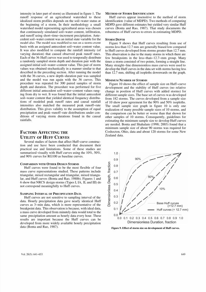
Figure 9 shows that Huff curves resulting from use of storms less than 12.7 mm are generally biased low compared

to Huff curves developed from storms greater than 12.7 mm.This observation is due to the many storms in which there arefew breakpoints in the less−than−12.7−mm group. Manytimes a storm consisted of two points, forming a straight line.Many straight−line dimensionless mass curves were used todevelop the Huff curves in the data set with storms having lessthan 12.7 mm, shifting all isopleths downwards on the graph.

MINIMUM NUMBER OF STORMS

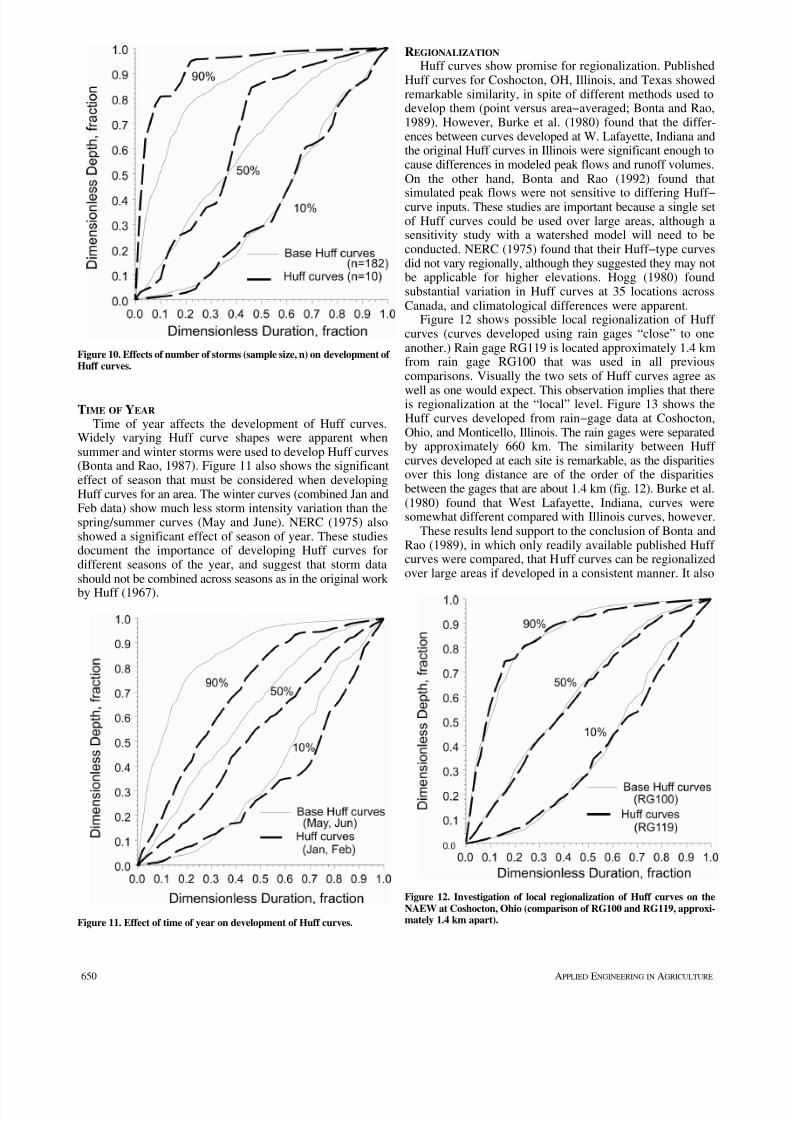
Figure 10 shows the effect of sample size on Huff−curvedevelopment and the stability of Huff curves (no relativechange in position of Huff curves with added storms) fordifferent sample sizes. The base set of curves was developedfrom 182 storms. The curves developed from a sample size

of 10 show poor agreement for the 90% and 50% isopleths.The small sample size graph in figure 10 is only onerealization of many possible sample sizes of 10 storms, andthe comparison can be better or worse than that shown forother samples of 10 storms. Consequently, guidelines forestimating the minimum sample size to develop Huff curvesare needed. Bonta and Shahalam (1998; 2003) found that aminimum sample size of about 90 storms was required forCoshocton, Ohio, data and about 120 storms for some NewZealand data.

Figure 9. Effect of storm size on development of Huff curves.




Figure 10. Effects of number of storms (sample size, n) on development of Huff curves.

TIME OF YEAR

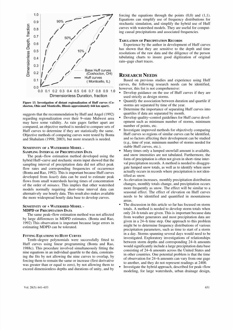
Time of year affects the development of Huff curves.Widely varying Huff curve shapes were apparent whensummer and winter storms were used to develop Huff curves(Bonta and Rao, 1987). Figure 11 also shows the significanteffect of season that must be considered when developingHuff curves for an area. The winter curves (combined Jan andFeb data) show much less storm intensity variation than thespring/summer curves (May and June). NERC (1975) alsoshowed a significant effect of season of year. These studiesdocument the importance of developing Huff curves fordifferent seasons of the year, and suggest that storm datashould not be combined across seasons as in the original work

by Huff (1967).

Figure 11. Effect of time of year on development of Huff curves.

REGIONALIZATION

Huff curves show promise for regionalization. PublishedHuff curves for Coshocton, OH, Illinois, and Texas showedremarkable similarity, in spite of different methods used todevelop them (point versus area−averaged; Bonta and Rao,1989). However, Burke et al. (1980) found that the differ-ences between curves developed at W. Lafayette, Indiana andthe original Huff curves in Illinois were significant enough tocause differences in modeled peak flows and runoff volumes.On the other hand, Bonta and Rao (1992) found that

simulated peak flows were not sensitive to differing Huff−curve inputs. These studies are important because a single setof Huff curves could be used over large areas, although asensitivity study with a watershed model will need to beconducted. NERC (1975) found that their Huff−type curvesdid not vary regionally, although they suggested they may notbe applicable for higher elevations. Hogg (1980) foundsubstantial variation in Huff curves at 35 locations acrossCanada, and climatological differences were apparent.

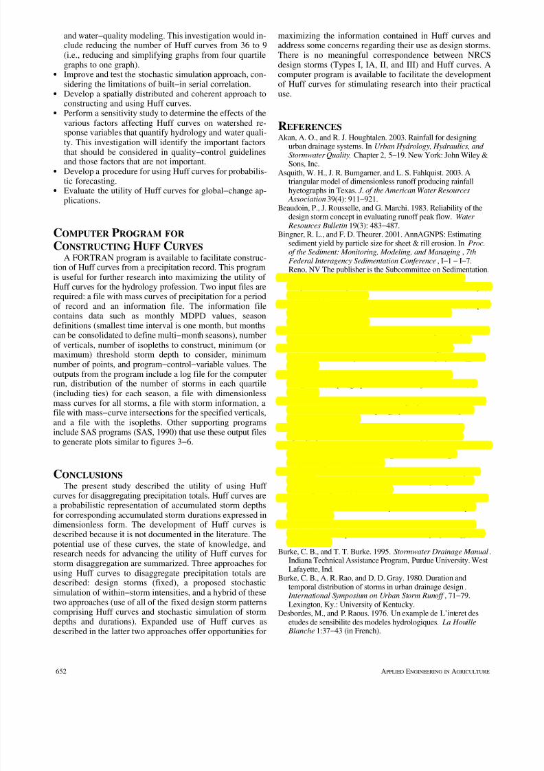
Figure 12 shows possible local regionalization of Huff curves (curves developed using rain gages “close” to oneanother.) Rain gage RG119 is located approximately 1.4 kmfrom rain gage RG100 that was used in all previouscomparisons. Visually the two sets of Huff curves agree as

well as one would expect. This observation implies that thereis regionalization at the “local” level. Figure 13 shows theHuff curves developed from rain−gage data at Coshocton,Ohio, and Monticello, Illinois. The rain gages were separatedby approximately 660 km. The similarity between Huff curves developed at each site is remarkable, as the disparitiesover this long distance are of the order of the disparitiesbetween the gages that are about 1.4 km (fig. 12). Burke et al.(1980) found that West Lafayette, Indiana, curves weresomewhat different compared with Illinois curves, however.

These results lend support to the conclusion of Bonta andRao (1989), in which only readily available published Huff curves were compared, that Huff curves can be regionalizedover large areas if developed in a consistent manner. It also

Figure 12. Investigation of local regionalization of Huff curves on theNAEW at Coshocton, Ohio (comparison of RG100 and RG119, approxi-mately 1.4 km apart).



651Vol. 20(5): 641−653

Figure 13. Investigation of distant regionalization of Huff curves (Co-shocton, Ohio and Monticello, Illinois approximately 644 km apart).

suggests that the recommendation by Huff and Angel (1992)regarding regionalization over their 9−state Midwest areamay have some validity. As rain gages farther apart arecompared, an objective method is needed to compare sets of Huff curves to determine if they are statistically the same.Objective methods of comparing curves were tested by Bontaand Shahalam (1998; 2003), but more research is needed.

SENSITIVITY OF A WATERSHED MODEL – SAMPLING INTERVAL OF PRECIPITATION DATA

The peak−flow estimation method developed using thehybrid Huff−curve and stochastic storm input showed that thesampling interval of precipitation data did not affect peak flow rates and corresponding frequencies of occurrence

(Bonta and Rao, 1992). This is important because Huff curvesdeveloped from hourly data can be used to estimate peak flows from small watersheds having times of concentrationof the order of minutes. This implies that other watershedmodels normally requiring short−time interval data canalternatively use hourly data. This result also makes availablethe more widespread hourly data base to develop curves.

SENSITIVITY OF A WATERSHED MODEL – MDPD OF PRECIPITATION DATA

The same peak−flow estimation method was not affectedby large differences in MDPD estimates. (Bonta and Rao,1992) This observation is important because large errors inestimating MDPD can be tolerated.

FITTING EQUATIONS TO HUFF CURVES

Tenth−degree polynomials were successfully fitted toHuff curves using linear programming (Bonta and Rao,1988c). This procedure involved simultaneously fitting thenine equations in an individual quartile to the data, constrain-ing the fits by not allowing the nine curves to overlap, byforcing them to remain the same or increase (first derivativewas greater than or equal to zero), by not allowing them toexceed dimensionless depths and durations of unity, and by

forcing the equations through the points (0,0) and (1,1).Equations can simplify use of frequency distributions forstochastic simulation, and simplify the hybrid use of Huff curves with watershed models. They are useful for comput-ing causal precipitations and associated frequencies.

TABULATION OF PRECIPITATION RECORDS

Experience by the author in development of Huff curveshas shown that they are sensitive to the depth and timeresolutions of the raw data and the diligence of the person

tabulating charts to insure good digitization of originalrain−gage chart traces.

RESEARCH NEEDS

Based on previous studies and experience using Huff curves, the following research needs can be identified,however, this list is not comprehensive:S Develop guidance on the use of Huff curves if they are

used strictly as design storms.S Quantify the association between duration and quartile if

storms are separated by time of the year.S Determine the importance of separating Huff curves into

quartiles if data are separated by month.S Develop quality−control guidelines for Huff curve devel-

opment such as minimum number of storms, minimumnumber of points, etc.

S Investigate improved methods for objectively comparingHuff curves so regions of similar curves can be identified,and so factors affecting their development can be studied(e.g., time of year, minimum number of storms needed forstable Huff curves, etc.).

S Many times only a lumped snowfall amount is available,and snow intensities are not tabulated. Furthermore, theform of precipitation is often not given in short−time inter-val precipitation records. A method is needed to disaggre-gate lumped snow totals, as well as to identify when snowactually occurs in records where precipitation is not iden-tified as snow.

S As elevation increases, monthly precipitation distributionchanges, monthly totals change, and precipitation occursmore frequently as snow. The effect will be similar to aseasonal effect. The effect of elevation on Huff curvesneeds to be identified and quantified in mountainousareas.

S The discussion in this article so far has focused on stormtotals. A method is needed to develop storm totals whenonly 24−h totals are given. This is important because datafrom weather generators and most precipitation data aregiven in a 24−h time step. One approach to this problemmight be to determine frequency distributions of various

precipitation parameters, such as time to start of a stormin a day. Storms spanning several days would need to beinvestigated. Exploratory investigations of relationshipsbetween storm depths and corresponding 24−h amountswould significantly include a large precipitation data baseconsisting of 24−h amounts across the United States andin other countries. One potential problem is that the timeof observation for 24−h amounts can vary from one gageto another, and they do not represent readings at 2400.

S Investigate the hybrid approach, described for peak−flowmodeling, for large watersheds, urban drainage design,




and water−quality modeling. This investigation would in-clude reducing the number of Huff curves from 36 to 9(i.e., reducing and simplifying graphs from four quartilegraphs to one graph).

S Improve and test the stochastic simulation approach, con-sidering the limitations of built−in serial correlation.

S Develop a spatially distributed and coherent approach toconstructing and using Huff curves.

S Perform a sensitivity study to determine the effects of thevarious factors affecting Huff curves on watershed re-

sponse variables that quantify hydrology and water quali-ty. This investigation will identify the important factorsthat should be considered in quality−control guidelinesand those factors that are not important.

S Develop a procedure for using Huff curves for probabilis-tic forecasting.

S Evaluate the utility of Huff curves for global−change ap-plications.

COMPUTER PROGRAM FOR CONSTRUCTING HUFF CURVES

A FORTRAN program is available to facilitate construc-

tion of Huff curves from a precipitation record. This programis useful for further research into maximizing the utility of Huff curves for the hydrology profession. Two input files arerequired: a file with mass curves of precipitation for a periodof record and an information file. The information filecontains data such as monthly MDPD values, seasondefinitions (smallest time interval is one month, but monthscan be consolidated to define multi−month seasons), numberof verticals, number of isopleths to construct, minimum (ormaximum) threshold storm depth to consider, minimumnumber of points, and program−control−variable values. Theoutputs from the program include a log file for the computerrun, distribution of the number of storms in each quartile(including ties) for each season, a file with dimensionless

mass curves for all storms, a file with storm information, afile with mass−curve intersections for the specified verticals,and a file with the isopleths. Other supporting programsinclude SAS programs (SAS, 1990) that use these output filesto generate plots similar to figures 3−6.

CONCLUSIONS

The present study described the utility of using Huff curves for disaggregating precipitation totals. Huff curves area probabilistic representation of accumulated storm depthsfor corresponding accumulated storm durations expressed indimensionless form. The development of Huff curves isdescribed because it is not documented in the literature. Thepotential use of these curves, the state of knowledge, andresearch needs for advancing the utility of Huff curves forstorm disaggregation are summarized. Three approaches forusing Huff curves to disaggregate precipitation totals aredescribed: design storms (fixed), a proposed stochasticsimulation of within−storm intensities, and a hybrid of thesetwo approaches (use of all of the fixed design storm patternscomprising Huff curves and stochastic simulation of stormdepths and durations). Expanded use of Huff curves asdescribed in the latter two approaches offer opportunities for

maximizing the information contained in Huff curves andaddress some concerns regarding their use as design storms.There is no meaningful correspondence between NRCSdesign storms (Types I, IA, II, and III) and Huff curves. Acomputer program is available to facilitate the developmentof Huff curves for stimulating research into their practicaluse.

REFERENCES

Akan, A. O., and R. J. Houghtalen. 2003. Rainfall for designingurban drainage systems. In Urban Hydrology, Hydraulics, and Stormwater Quality, Chapter 2, 5−19. New York: John Wiley &Sons, Inc.

Asquith, W. H., J. R. Bumgarner, and L. S. Fahlquist. 2003. Atriangular model of dimensionless runoff producing rainfallhyetographs in Texas. J. of the American Water Resources

Association39(4): 911−921.Beaudoin, P., J. Rousselle, and G. Marchi. 1983. Reliability of the

design storm concept in evaluating runoff peak flow. Water Resources Bulletin 19(3): 483−487.

Bingner, R. L., and F. D. Theurer. 2001. AnnAGNPS: Estimatingsediment yield by particle size for sheet & rill erosion. In Proc.of the Sediment: Monitoring, Modeling, and Managing, 7thFederal Interagency Sedimentation Conference, I−1 − I−7.

Reno, NV The publisher is the Subcommittee on Sedimentation.Bonta, J. V. 2001. Characterizing and estimating spatial and

temporal variability of times between storms. Transactions of the

ASAE 44(6): 1593−1601.Bonta, J. V. 2004. Stochastic simulation of storm occurrence, depth,

duration, and within−storm intensities. Submitted toTransactions of the ASAE

Bonta, J. V., and A. R. Rao. 1987. Factors affecting development of Huff curves. Transactions of the ASAE 30(6): 1689−1693.

Bonta, J. V., and A. R. Rao. 1988a. Factors affecting theidentification of independent storm events. J. of Hydrology 98:275−293.

Bonta, J. V., and A. R. Rao. 1988b. Comparison of fourdesign−storm hyetographs. Transactions of the ASAE 31(1):102−106.

Bonta, J. V., and A. R. Rao. 1988c. Fitting equations to families of dimensionless cumulative hyetographs. Transactions of the ASAE 31(3): 756−760.

Bonta, J. V., and A. R. Rao. 1989. Regionalization of stormhyetographs. Water Resources Bulletin 25(1): 211−217.

Bonta, J. V., and A. R. Rao. 1992. Estimating peak flows from smallagricultural watersheds. J. of Irrigation and Drainage

Engineering 118(1): 122−137.Bonta, J. V., and A. R. Rao. 1994. Seasonal distributions of peak

flows from small agricultural watersheds. J. of Irrigation & Drainage Eng. 120(2): 422−439.

Bonta, J. V., and A. Shahalam. 1998. Investigation of techniques tocompare Huff curves. ASAE Paper No. 982192. St. Joseph,Mich.: ASAE.

Bonta, J. V., and A. Shahalam. 2003. Cumulative storm rainfalldistributions: comparison of Huff curves. J. of Hydrology (NZ)

42(1): 65−74.Burke, C. B., and T. T. Burke. 1995. Stormwater Drainage Manual.

Indiana Technical Assistance Program, Purdue University. WestLafayette, Ind.

Burke, C. B., A. R. Rao, and D. D. Gray. 1980. Duration andtemporal distribution of storms in urban drainage design.

International Symposium on Urban Storm Runoff , 71−79.Lexington, Ky.: University of Kentucky.

Desbordes, M., and P. Raous. 1976. Un example de L’interet desetudes de sensibilite des modeles hydrologiques. La Houille

Blanche 1:37−43 (in French).



653Vol. 20(5): 641−653

Grace, R. A., and P. S. Eagleson. 1966. The synthesis of short−timeincrement rainfall sequences. Massachusetts Institute of Technology, Hydrodynamics Laboratory, Report No. 91. Schoolof Civil Engineering, Massachusetts Institute of Technology,Cambridge, Mass.

Haestad Methods, 2003. Stormwater Conveyance Modeling and Design, First Edition. Waterbury, Conn.: Haestad Methods.

Hanson, C. L., H. B. Osborn, and D. A. Woolhiser. 1989. Dailyprecipitation simulation model for mountainous areas.Transactions of the ASAE 32(3): 865−873.

Hanson, C. L., G. L. Johnson, and W. L. Frymire. 2002. The GEM

(Generation of weather Elements for Multiple applications)weather simulation model. In 13th AMS Conf. Appl.Climatology, 117−121. American Meteorological Society,Portland, Oregon

Hanson, C. L., K. A. Cumming, D. A. Woolhiser, and C. W.Richardson. 1994. Microcomputer program for daily weathersimulation. U.S. Dept. Agric., Agric. Res. Svc. Pub. No.ARS−114. Washington, D.C.

Hjelmfelt, A. T. 1980. Time distribution of clock hour rainfall. InCREAMS, A field scale model for chemicals, runoff, anderosion from agricultural management systems. USDA,Conservation Research Report No. 26. Washington, D.C.

Hogg, W. D. 1980. Time distribution of short duration stormrainfall in Canada. Proc. of the Canadian HydrologySymposium: Hydrology of Developed Areas, Toronto, National

Research Council, 53−63. Ottawa, Ontario: NRC.Huff, F. A. 1967. Time distribution of rainfall in heavy storms.

Water Resources Research 3(4): 1007−1019.Huff, F. A. 1990. Time distributions of heavy rainstorms in Illinois.

Illinois State Water Survey, Circular 173. Champaign, Ill.Huff, F. A., and J. R. Angel, 1989. Rainfall distributions and

hydroclimatic characteristics of heavy rainstorms in Illinois(Bulletin 70). Illinois State Water Survey. Champaign, Ill.

Huff, F. A., and J. R. Angel. 1992. Rainfall frequency atlas of theMidwest. Illinois State Water Survey, Champaign, Ill.

Huff, F. A., and J. L. Vogel. 1976. Hydrometeorology of heavyrainstorms in Chicago and Northeastern Illinois. Illinois StateWater Survey Report of Investigation 82. Champaign, Ill.

Intergovernmental Panel on Climate Change. 1990. Climate

Change: The IPCC Scientific Assessment,eds.J. T. Houghton, G.J. Jenkins, and J. J. Ephraums. Cambridge: University Press.

Keifer, C. J., and H. H. Chu. 1957. Synthetic storm pattern fordrainage design. J. of the Hydraulics Divison, ASCE 83(HY4):1−25.

Natural Environment Research Council (NERC). 1975. Flood Studies Report, Vol. 2.Meteorological studies. Whitefriars PressLtd., London.

Nicks, A. D., L. J. Lane, and G. A. Gander. 1995. Chapter 2.Weather Generator. In Hillslope Profile and Watershed Model

Documentation, eds. D. C. Flanagan and M. A. Nearing.NSERL Report No. 10, USDA−ARS National Soil ErosionResearch Laboratory, West Lafayette, Ind.

Patry, G., and M. B. McPherson. 1979. The Design Storm Concept.Urban Water Resources Research Group. Proc. of a seminar atEcole Polytechnique de Montreal Montreal, Quebec.

Pilgrim, D. H., I. Cordery, and R. French. 1969. Temporal patternsof design rainfall for Sydney. Civil Engineering Transactions,

Institution of Engineers, Australia CE11(1): 9−14.

Pilgrim, D. H., and I. Cordery. 1975. Rainfall temporal patterns fordesign floods. J. of the Hydraulics Division HY1: 81−95.Purdue, A. M., G. D. Jeong, and A. R. Rao. 1992. Statistical

characteristics of short time increment rainfall. School of CivilEngineering, Purdue University, No. CE−EHE−92−09. WestLafayette, Ind.

Rao, R. A., and B. T. Chenchayya. 1974. Probabilistic analysis andsimulation of the short time increment rainfall process. PurdueUniversity Water Resources Research Center, Technical ReportNo. 55. West Lafayette, Ind.

Restrepo, P. J., and P. S. Eagleson. 1982. Identification of independent rainstorms. J. Hydrol. 55: 303−319.

SAS Institute Inc. 1990. SAS/GRAPH R Software: Reference,Version 6, First Ed., Vol. 2. Cary, N.C.: SAS Institute Inc.

Sifalda, V. 1973. Entwicklung eines Berechnungsregens für dieBemessung von Kanalnetzen. Gwf−wasser/Abwasser 114(9):435−440 (in German).

Soil Conservation Service (SCS). 1986. Urban hydrology for smallwatersheds. Technical Release 55, U.S. Department of Agriculture, Washington, D.C.

Sutherland, F. R. 1982. An improved rainfall intensity distributionfor hydrograph synthesis. Univ. of the Witwatersrand, Dept. of Civil Engineering, Johannesburg, South Africa Report No.1/1983.

Terstriep, M. L., and J. B. Stall. 1974. The Illinois urban drainagearea simulator, ILLUDAS. Illinois State Water Survey Bulletin58. Champaign, Ill.

Wenzel, H. G., Jr., and M. L. Voorhees. 1981. An evaluation of theurban design storm concept. University of Illinois atUrbana−Champaign, Water Resources Center, Research Report164. Urbana−Champaign, Ill.

Yen, B. C., and V. T. Chow. 1980. Design hyetographs for smalldrainage structures. J. of the Hydraulics Division, ASCE 106(HY6): 1055−1076.

Zeleke, G., T. Winter, and D. Flanagan. 2000. BPCDG: Breakpointclimate data generator for WEPP using observed standardweather data sets. USDA−ARS Natl. Soil Erosion Res. Lab,http://topsoil.nserl.purdue.edu/nserlweb/weppmain/BPCDG.html (accessed 11/24/2003).

bonta desarrollo jy utilidad de la curva de huff

Documents