biblioteca digital | fcen-uba | ubalde, sebastián. 2016 03 22
TRANSCRIPT

Reconocimiento de acciones en videos deprofundidad
Ubalde, Sebastián2016 03 22
Tesis Doctoral
Facultad de Ciencias Exactas y NaturalesUniversidad de Buenos Aires
www.digital.bl.fcen.uba.ar
Contacto: [email protected]
Este documento forma parte de la colección de tesis doctorales y de maestría de la BibliotecaCentral Dr. Luis Federico Leloir. Su utilización debe ser acompañada por la cita bibliográfica conreconocimiento de la fuente.
This document is part of the doctoral theses collection of the Central Library Dr. Luis Federico Leloir.It should be used accompanied by the corresponding citation acknowledging the source.
Fuente / source: Biblioteca Digital de la Facultad de Ciencias Exactas y Naturales - Universidad de Buenos Aires

Universidad de Buenos Aires
Facultad de Ciencias Exctas y Naturales
Departamento de Computacion
Reconocimiento de acciones en videos de
profundidad
Tesis presentada para optar al tıtulo de Doctor de la Universidad de
Buenos Aires en el area Cs. de la Computacion
Sebastian UBALDE
Directora de tesis: Marta E. Mejail
Consejera de estudios: Marta E. Mejail
Buenos Aires, 2015


Reconocimiento de acciones en videos de profundidad
Resumen El problema de reconocer automaticamente una accion lleva-
da a cabo en un video esta recibiendo mucha atencion en la comunidad de
vision por computadora, con aplicaciones que van desde el reconocimiento
de personas hasta la interaccion persona-computador. Podemos pensar al
cuerpo humano como un sistema de segmentos rıgidos conectados por arti-
culaciones, y al movimiento del cuerpo como una transformacion continua
de la configuracion espacial de dichos segmentos. La llegada de camaras
de profundidad de bajo costo hizo posible el desarrollo de un algoritmo de
seguimiento de personas preciso y eficiente, que obtiene la ubicacion 3D de
varias articulaciones del esqueleto humano en tiempo real. Esta tesis presen-
ta contribuciones al modelado de la evolucion temporal de los esqueletos.
El modelado de la evolucion temporal de descriptores de esqueleto plan-
tea varios desafıos. En primer lugar, la posicion 3D estimada para las ar-
ticulaciones suele ser imprecisa. En segundo lugar, las acciones humanas
presentan gran variabilidad intra-clase. Esta variabilidad puede encontrarse
no solo en la configuracion de los esqueletos por separado (por ejemplo, la
misma accion da lugar a diferentes configuraciones para diestros y para zur-
dos) sino tambien en la dinamica de la accion: diferentes personas pueden
ejecutar una misma accion a distintas velocidades; las acciones que involu-
cran movimientos periodicos (como aplaudir) pueden presentar diferentes
cantidades de repeticiones de esos movimientos; dos videos de la misma
accion puede estar no-alineados temporalmente; etc. Por ultimo, acciones
diferentes pueden involucrar configuraciones de esqueleto y movimientos
similares, dando lugar a un escenario de gran similaridad inter-clase. En
este trabajo exploramos dos enfoques para hacer frente a estas dificultades.
En el primer enfoque presentamos una extension a Edit Distance on Real
sequence (EDR), una medida de similaridad entre series temporales robusta
y precisa. Proponemos dos mejoras clave a EDR: una funcion de costo suave
para el alineamiento de puntos y un algoritmo de alineamiento modifica-

3
do basado en el concepto de Instancia-a-Clase (I2C, por el termino en ingles:
Instance-to-Class) . La funcion de distancia resultante tiene en cuenta el or-
denamiento temporal de las secuencias comparadas, no requiere aprendi-
zaje de parametros y es altamente tolerante al ruido y al desfasaje temporal.
Ademas, mejora los resultados de metodos no-parametricos de clasificacion
de secuencias, sobre todo en casos de alta variabilidad intra-clase y pocos
datos de entrenamiento.
En el segundo enfoque, reconocemos que la cantidad de esqueletos dis-
criminativos en una secuencia puede ser baja. Los esqueletos restantes pue-
den ser ruidosos, tener configuraciones comunes a varias acciones (por ejem-
plo, la configuracion correspondiente a un esqueleto sentado e inmovil) u
ocurrir en instantes de tiempo poco comunes para la accion del video. Por lo
tanto, el problema puede ser naturalmente encarado como uno de Aprendi-
zaje Multi Instancia (MIL por el termino en ingles Multiple Instance Learning).
En MIL, las instancias de entrenamiento se organizan en conjuntos o bags.
Cada bag de entrenamiento tiene asignada una etiqueta que indica la clase
a la que pertenece. Un bag etiquetado con una determinada clase contiene
instancias que son caracterısticas de la clase, pero puede (y generalmente
ası ocurre) tambien contener instancias que no lo son. Siguiendo esta idea,
representamos los videos como bags de descriptores de esqueleto con mar-
cas de tiempo, y proponemos un framework basado en MIL para el reco-
nocimiento de acciones. Nuestro enfoque resulta muy tolerante al ruido, la
variabilidad intra-clase y la similaridad inter-clase. El framework propuesto
es simple y provee un mecanismo claro para regular la tolerancia al ruido, a
la poca alineacion temporal y a la variacion en las velocidades de ejecucion.
Evaluamos los enfoques presentados en cuatro bases de datos publicas
capturadas con camaras de profundidad. En todos los casos, se trata de
bases desafiantes. Los resultados muestran una comparacion favorable de
nuestras propuestas respecto al estado del arte.
Palabras clave: Video de profundidad, Aprendizaje Multi Instancia, Citation-
kNN, Edit Distance on Real sequence, Instancia-a-Clase
3


Action recognition in depth videos
Abstract The problem of automatically identifying an action performed
in a video is receiving a great deal of attention in the computer vision com-
munity, with applications ranging from people recognition to human com-
puter interaction. We can think the human body as an articulated system
of rigid segments connected by joints, and human motion as a continuous
transformation of the spatial arrangement of those segments. The arrival of
low-cost depth cameras has made possible the development of an accurate
and efficient human body tracking algorithm, that computes the 3D loca-
tion of several skeleton joints in real time. This thesis presents contributions
concerning the modeling of the skeletons temporal evolution.
Modeling the temporal evolution of skeleton descriptors is a challenging
task. First, the estimated location of the 3D joints are usually inaccurate.
Second, human actions have large intra-class variability. This variability
may be found not only in the spatial configuration of individual skeletons
(for example, the same action involves different configurations for right-
handed and left-handed people) but also on the action dynamics: different
people have different execution speeds; actions with periodic movements
(like clapping) may involve different numbers of repetitions; two videos of
the same action may be temporally misaligned; etc. Finally, different actions
may involve similar skeletal configurations, as well as similar movements,
effectively yielding large inter-class similarity. We explore two approaches
to the problem that aim at tackling this difficulties.
In the first approach, we present an extension to the Edit Distance on
Real sequence (EDR), a robust and accurate similarity measure between time
series. We introduce two key improvements to EDR: a weighted matching
scheme for the points in the series and a modified aligning algorithm based
on the concept of Instance-to-Class distance. The resulting distance function
takes into account temporal ordering, requires no learning of parameters
and is highly tolerant to noise and temporal misalignment. Furthermore,

6
it improves the results of non-parametric sequence classification methods,
specially in cases of large intra-class variability and small training sets.
In the second approach, we explicitly acknowledge that the number of
discriminative skeletons in a sequence might be low. The rest of the skele-
tons might be noisy or too person-specific, have a configuration common to
several actions (for example, a sit still configuration), or occur at uncommon
frames. Thus, the problem can be naturally treated as a Multiple Instance
Learning (MIL) problem. In MIL, training instances are organized into bags.
A bag from a given class contains some instances that are characteristic of
that class, but might (and most probably will) contain instances that are not.
Following this idea, we represent videos as bags of time-stamped skeleton
descriptors, and we propose a new MIL framework for action recognition
from skeleton sequences. We found that our approach is highly tolerant to
noise, intra-class variability and inter-class similarity. The proposed frame-
work is simple and provides a clear way of regulating tolerance to noise,
temporal misalignment and variations in execution speed.
We evaluate the proposed approaches on four publicly available chal-
lenging datasets captured by depth cameras, and we show that they com-
pare favorably against other state-of-the-art methods.
Keywords: Depth video, Multiple Instance Learning, Citation-kNN, Edit
Distance on Real sequence, Instance-to-Class
6


Contents
1 Introduction 16
1.1 Problem description . . . . . . . . . . . . . . . . . . . . . . . . 17
1.1.1 Action recognition in depth videos . . . . . . . . . . . . 18
1.2 Contributions . . . . . . . . . . . . . . . . . . . . . . . . . . . . 22
1.3 Publications . . . . . . . . . . . . . . . . . . . . . . . . . . . . . 23
1.4 Organization of the thesis . . . . . . . . . . . . . . . . . . . . . 25
1 Introduccion 26
1.1 Descripcion del problema . . . . . . . . . . . . . . . . . . . . . 27
1.1.1 Reconocimiento de acciones en videos de profundidad 29
1.2 Contribuciones . . . . . . . . . . . . . . . . . . . . . . . . . . . 33
1.3 Publicaciones . . . . . . . . . . . . . . . . . . . . . . . . . . . . 34
1.4 Organizacion de la tesis . . . . . . . . . . . . . . . . . . . . . . 36
2 Prior works and datasets 37
2.1 Related Work . . . . . . . . . . . . . . . . . . . . . . . . . . . . 37
2.1.1 Skeleton-based action recognition review . . . . . . . . 37
2.2 Datasets . . . . . . . . . . . . . . . . . . . . . . . . . . . . . . . 43
2.2.1 MSRDailyActivity3D dataset . . . . . . . . . . . . . . . 44
2.2.2 MSRAction3D dataset . . . . . . . . . . . . . . . . . . . 45
2.2.3 UTKinect dataset . . . . . . . . . . . . . . . . . . . . . . 46
2.2.4 Florence3D dataset . . . . . . . . . . . . . . . . . . . . . 48
2.3 Resumen . . . . . . . . . . . . . . . . . . . . . . . . . . . . . . . 49

CONTENTS 9
3 Action recognition using Instance-to-Class Edit Distance on Real
sequence 50
3.1 Introduction . . . . . . . . . . . . . . . . . . . . . . . . . . . . . 50
3.2 Recognizing actions using Instance-to-Class
Edit Distance on Real sequence . . . . . . . . . . . . . . . . . . 53
3.2.1 Comparing time series . . . . . . . . . . . . . . . . . . . 54
3.2.2 A new time series similarity measure . . . . . . . . . . 62
3.2.3 Action recognition with I2CEDR . . . . . . . . . . . . . 74
3.3 Results . . . . . . . . . . . . . . . . . . . . . . . . . . . . . . . . 80
3.3.1 Evaluation of the proposed EDR extensions . . . . . . . 80
3.3.2 Comparison of the proposed EDR extensions with other
elastic matching similarity measures . . . . . . . . . . . 82
3.3.3 Robustness analysis . . . . . . . . . . . . . . . . . . . . 84
3.3.4 Comparison with the state-of-the-art . . . . . . . . . . . 87
3.4 Resumen . . . . . . . . . . . . . . . . . . . . . . . . . . . . . . . 89
4 Action recognition using Citation-kNN on bags of time-stamped
poses 91
4.1 Introduction . . . . . . . . . . . . . . . . . . . . . . . . . . . . . 91
4.2 Recognizing actions with Citation-kNN on bags of time-stamped
poses . . . . . . . . . . . . . . . . . . . . . . . . . . . . . . . . . 93
4.2.1 Multiple Instance Learning . . . . . . . . . . . . . . . . 93
4.2.2 Citation-kNN . . . . . . . . . . . . . . . . . . . . . . . . 94
4.2.3 Modified Citation-kNN . . . . . . . . . . . . . . . . . . 98
4.2.4 Citation-kNN on bags of time-stamped poses . . . . . 99
4.3 Results . . . . . . . . . . . . . . . . . . . . . . . . . . . . . . . . 111
4.3.1 Parameter selection . . . . . . . . . . . . . . . . . . . . . 111
4.3.2 Parameter influence . . . . . . . . . . . . . . . . . . . . 112
4.3.3 Evaluation of the main components of the action recog-
nition procedure . . . . . . . . . . . . . . . . . . . . . . 116
4.3.4 Robustness analysis . . . . . . . . . . . . . . . . . . . . 118
4.3.5 Comparation with the state-of-the-art . . . . . . . . . . 123
4.4 Resumen . . . . . . . . . . . . . . . . . . . . . . . . . . . . . . . 125
9

CONTENTS 10
5 Conclusions and perspective 127
5 Conclusiones y perspectiva 130
Bibliography 133
10

List of Figures
1.1 Four examples of the challenges involved in RGB-based ac-
tion recognition. Figures 1.1a and 1.1b show frames of videos
that have quite different appearance despite being instances
of the same action. Figures 1.1c and 1.1d show frames of
videos that have similar appearance even though they cor-
respond to different actions. See text for details. . . . . . . . . 19
1.2 RGB (1.2a) and depth (1.2b) sequences for an instance of the
cheer up action. . . . . . . . . . . . . . . . . . . . . . . . . . . . . 19
1.3 Two widely used depth devices: Microsoft Kinect (1.3a) and
Asus Xtion PRO LIVE (1.3b). . . . . . . . . . . . . . . . . . . . . 20
1.4 Joints tracked by Kinect. . . . . . . . . . . . . . . . . . . . . . . 21
1.1 Cuatro ejemplos de los desafıos involucrados en el recono-
cimiento de acciones basado en RGB. Las figuras 1.1a y 1.1b
muestran frames de videos que tienen apariencia consider-
ablemente diferente a pesar de ser instancias de la misma ac-
cion. Las figuras 1.1c y 1.1d muestran frames de videos que
tienen apariencia similar pese a que corresponden a acciones
diferentes. Ver el texto para mas detalles. . . . . . . . . . . . . 29
1.2 Secuencias de frames RGB (1.2a) y de profundidad (1.2b) para
una instancia de la accion cheer up. . . . . . . . . . . . . . . . . 30
1.3 Dos sensores de profundidad ampliamente utilizados: Mi-
crosoft Kinect (1.3a) y Asus Xtion PRO LIVE (1.3b). . . . . . . 30
1.4 Articulaciones localizadas por Kinect. . . . . . . . . . . . . . . 31

LIST OF FIGURES 12
2.1 Example RGB frames of the MSRDailyActivity3D dataset. . . 45
2.2 Example depth frames of the MSRAction3D dataset. . . . . . . 46
2.3 Example frames of the UTKinect dataset. . . . . . . . . . . . . 47
2.4 Example frames of the Florence3D dataset. . . . . . . . . . . . 48
3.1 A schematic example of a warping path. . . . . . . . . . . . . . 56
3.2 A schematic example of a trace. . . . . . . . . . . . . . . . . . . 60
3.3 A schematic example of an extended trace. . . . . . . . . . . . 68
3.4 Traces and EDRS distances between a query sequence A and
two training sequences C11 (3.4a) and C1
2 (3.4b). The computed
distances are larger than expected. See text for description. . . 70
3.5 Traces and EDRS distances between a query sequence A and
two training sequences C21 (3.5a) and C2
2 (3.5b). See text for
description. . . . . . . . . . . . . . . . . . . . . . . . . . . . . . 71
3.6 Extended traces and I2CEDR distances between a query se-
quence A and two sets of training sequences C1 and C2. See
text for description. . . . . . . . . . . . . . . . . . . . . . . . . . 72
3.7 Evaluation of the proposed EDR extensions. The original
EDR distance is referred to as Hard, while Soft and I2C de-
note EDRS and I2CEDR respectively. The term I2C-P denotes
the use of I2CEDR combined with the multi-part approach.
See text for details. . . . . . . . . . . . . . . . . . . . . . . . . . 81
3.8 Comparison of I2CEDR with other elastic matching similar-
ity measures. The presented functions EDRS (referred as EDR
Soft) and I2CEDR (referred as I2C-EDR) are compared with
four other measures: Frechet, Dynamic Time Warping (DTW),
Instance-to-Class Frechet (I2C-Frechet) and Instance-to-Class
Dynamic Time Warping (I2C-DTW). See text for details. . . . . 83
3.9 Relationship between the relative accuracy and the noise stan-
dard variation for several methods on two datasets: MSRDai-
lyActivity3D (3.9a) and UTKinect (3.9b). . . . . . . . . . . . . . 85
12

LIST OF FIGURES 13
3.10 Relationship between the relative accuracy and the temporal
misalignment for several methods on two datasets: MSRDai-
lyActivity3D (3.10a) and UTKinect (3.10b). . . . . . . . . . . . 86
4.1 The traditional kNN method for combining neighbors labels
to obtain the label of a query is not directly applicable to
the MIL setting. The figure illustrates how false positive in-
stances contained in positive bags attract negative bags. For
example, given {P1, P2, N1} as training bags, N2 will be clas-
sified as positive when the minimal Hausdorff distance is used. 97
4.2 Illustration of the Hausdorff distance between two bags of
skeleton descriptors, corresponding to the actions cheer up
and drink. Figure 4.2a describes the directed Hausdorff dis-
tance from the cheer up bag to the drink bag. Figure 4.2b de-
scribes the distances for the directed Hausdorff distance from
the drink bag to the cheer up bag. Each descriptor in the source
bag is linked by an arrow to its nearest neighbor in the target
bag. The distance to such nearest neighbor is indicated both
by the color of the arrow (following the color scale shown on
the right side) and by the number next to the arrow. See text
for details. . . . . . . . . . . . . . . . . . . . . . . . . . . . . . . 103
13

LIST OF FIGURES 14
4.3 Illustration of the Hausdorff distance between a query bag
and two training bags of skeleton descriptors. The query bag
corresponds to the action sit down. Training bags are labeled
with the actions sit down and stand up. Figure 4.3a describes
the directed Hausdorff distance from the stand up bag to the
query bag. Figure 4.3b describes the directed Hausdorff dis-
tance from the sit down training bag to the query bag. Tem-
poral order is not considered. Descriptors in the source bag
are linked by an arrow to their nearest neighbors in the target
bag. The distance to such nearest neighbor is indicated both
by the color of the arrow (following the color scale shown on
the right side) and by the number next to the arrow. See text
for details. . . . . . . . . . . . . . . . . . . . . . . . . . . . . . . 104
4.4 Illustration of the Hausdorff distance between a query bag
and two training bags of skeleton descriptors. The compared
bags are the same as in Figure 4.3. Different from the scenario
illustrated in that Figure, the example shown here takes into
account temporal information. See text for details. . . . . . . . 106
4.5 Illustration of the Hausdorff distance between a query bag
and two training bags of skeleton descriptors. The query bag
corresponds to the action cheer up. Training bags are labeled
with the actions cheer up and drink. Figure 4.5a describes
the directed Hausdorff distance from the cheer up bag to the
query bag. Figure 4.5b describes the directed Hausdorff dis-
tance from the query bag to the cheer up training bag. One
of the descriptors in the cheer up training bag is very noisy.
Descriptors in the source bag are linked by an arrow to their
nearest neighbors in the target bag. The distance to such near-
est neighbor is indicated both by the color of the arrow (fol-
lowing the color scale shown on the right side) and by the
number next to the arrow. See text for details. . . . . . . . . . . 108
4.6 Parameter influence for two of the four considered datasets. . 113
4.7 Parameter influence for two of the four considered datasets. . 114
14

LIST OF FIGURES 15
4.8 Confusion matrices for the UTKinect dataset. Figure 4.8a shows
the results obtained when time information is ignored. Figure
4.8b shows the results obtained when taking temporal infor-
mation into account. . . . . . . . . . . . . . . . . . . . . . . . . 119
4.9 Confusion matrices for the MSRDailyActivity3D dataset. In
Figure 4.9a time information is ignored, while in Figure 4.9b
it is not. . . . . . . . . . . . . . . . . . . . . . . . . . . . . . . . . 120
4.10 Relationship between the relative accuracy and the noise stan-
dard variation for several methods on two datasets: MSRDai-
lyActivity3D (4.10a) and UTKinect (4.10b). . . . . . . . . . . . 122
4.11 Relationship between the relative accuracy and the temporal
misalignment for several methods on two datasets: MSRDai-
lyActivity3D (4.11a) and UTKinect (4.11b). . . . . . . . . . . . 123
15

Chapter 1
Introduction
Action recognition is a growing topic in computer vision research. Gener-
ally speaking, it consists of identifying which of a predefined set of actions is
performed in a given video. The problem is usually approached using ma-
chine learning techniques, that tend to deal robustly with the complexities
found in real data.
Automatically identifying an action performed in a video can be a valu-
able tool in many applications. A common example is the analysis of surveil-
lance videos [Cha02]. Many security systems are based on the the data cap-
tured by several cameras. When the number of cameras is large, it can be
hard or even impossible for human controllers to manually detect important
events in the videos.
Closely related is the use of video understanding techniques for the pur-
pose of elderly and children care in indoor environments such as smart
homes and smart hospitals [SS15]. Monitoring and automatically recogniz-
ing daily activities can be of great help for assisting the residents, as well as
for describing their functional and health status. Yet another related appli-
cation is automatic video summarization, that provides short videos using
only the important scenes from the original video.
Another common example is content-based search in video databases
[HXL+11]. The ability to automatically obtain textual data describing a
video avoids the need for manual annotation, and can be crucial for the
development of more useful and informative datasets.

1.1 Problem description 17
Human-computer interaction is a further field that benefits from im-
provements in action recognition techniques. For example, such techniques
can be used to provide interfaces for people with motion impairments, eas-
ing their interaction with computers or other people [ZHJR11]. Another
common application is the development of video games that let the user
interact with the console/computer without the need for a game controller
[RKH11].
Behavior-based biometrics has also received much attention in the last
years. Unlike classical biometrics (such as fingerprints-based), they obtain
data for identification without interfering with the activity of the person.
A typical example is gait recognition [SPL+05]. A related use concerns the
automatic guidance of a patients movements in rehabilitation systems.
Therefore, new developments in action recognition methods, such as the
ones presented in this work, can be of great interest for a wide range of
applications.
1.1 Problem description
This thesis focus on the problem of action recognition from depth videos. In
this section, we give a general introduction to the problem and we clarify
several aspects about it. Specifically, we make explicit what we understand
by action recognition, and describe how the problem changes depending on
the type of video data employed. In doing so, we pay special attention to
depth data, as this is the one used in this work.
Given a list of possible actions and a video showing an actor performing
any one of them, the ultimate goal in the considered problem is to recog-
nize the action being performed. To clarify the meaning of the termn action,
the taxonomy defined in [MHK06] can be used. The work distinguishes
between action primitives (or movements), actions and activities. Action prim-
itives are atomic motions, and can be considered as the building blocks of
actions. Activities in turn are made up of several actions. As an example,
cooking can be thought of as an activity, involving several actions such as
chopping and stirring. Chopping can in turn be decomposed in several action
17

1.1 Problem description 18
primitives, such as taking a knife and cutting a vegetable. The actions con-
sidered in the thesis can be thought of as belonging to the action primitive
category. Note, however, that the granularity of the primitives may vary de-
pending on the application, and some of the actions considered in this work
can be very well seen as simple exemplars of the action category.
A large number of works have been proposed for action recognition from
RGB videos. This type of video data poses several challenges. On the one
hand, the appearance of an action can vary considerably in different videos.
This may be due to changes in lighting conditions, occlusions, viewpoint,
actor’s clothing, execution style, etc. Figures 1.1a and 1.1b show examples
of videos that have quite different appearance despite being instances of the
same action. The former corresponds to the action play game and the latter to
the action use vacuum cleaner. On the other hand, different actions can look
very similar to each other. This is illustrated in Figure 1.1c, that compares
frames from the actions drink and call cellphone. Another example of this
phenomena can be seen in Figure 1.1d, that shows frames from the actions
read and write.
The difficulties mentioned above have been partially mitigated with the
arrival of low cost depth sensors. Section 1.1.1 introduces some of the tech-
nologies used for depth sensing, and explain their advantages over tradi-
tional RGB videos. In particular, it highlights the possibility of inferring an
actor’s pose based on depth information, which is crucial for the methods
presented in the thesis.
1.1.1 Action recognition in depth videos
The advent of low cost depth sensors opened up new options to address
classical difficulties in action recognition. Typical depth sensors consist of
an infrared laser projector and an infrared camera. Combined, the camera
and the projector can be used to create a depth map, which encodes distance
information between the objects in the scene and the camera. Most of the
devices are also coupled with an RGB camera. Figure 1.2 shows three dif-
ferent RGB frames and their associated depth maps. Frames were extracted
18

1.1 Problem description 19
(a) (b)
(c) (d)
Figure 1.1: Four examples of the challenges involved in RGB-based action
recognition. Figures 1.1a and 1.1b show frames of videos that have quite
different appearance despite being instances of the same action. Figures 1.1c
and 1.1d show frames of videos that have similar appearance even though
they correspond to different actions. See text for details.
from a video corresponding to the cheer up action.
An example of this kind of technologies is the Microsoft Kinect. It calcu-
lates depth images at 320 × 240 or 640 × 480 resolution and at 30 frames
per second. See Figure 1.3a for a visual description of the device. An-
other widely used sensor is the Asus Xtion PRO LIVE, that offers either 60
320× 240 depth frames per second or 30 640× 480 depth frames per second.
The device is depicted in Figure 1.3b.
Many of the problems faced by RGB-based action recognitions methods
(a) (b)
Figure 1.2: RGB (1.2a) and depth (1.2b) sequences for an instance of the cheer
up action.
19

1.1 Problem description 20
IR projector
RGB cameraIR camera
(a)
IR projector
RGB camera
IR camera
(b)
Figure 1.3: Two widely used depth devices: Microsoft Kinect (1.3a) and
Asus Xtion PRO LIVE (1.3b).
are eased when working with depth videos. Such videos are less affected by
environmental conditions than conventional RGB data. More importantly,
they provide additional information that makes 3D reconstruction possible.
In particular, an accurate estimation of a person’s pose can be computed
from depth information, including the location of several skeleton joints at
each frame of a video. The temporal evolution of the human skeleton across
a video is a valuable tool for interpreting the action being performed. The
action recognition methods presented in this thesis are fully based on such
skeleton information. Therefore, in the following we describe how it can
be extracted from the raw depth data. Furthermore, we explain the specific
challenges involved in skeleton-based action recognition.
Skeleton-based action recognition
The current standard method for skeleton estimation from depth data is pre-
sented in the work of Shotton et al. [SSK+13]. The method labels each pixel
in a depth image as being either part of the human body, the background, or
unknown, and predicts the 3D position of several body joints (hand, wrist,
elbow, etc.). A description of the localized joints is shown in Fig. 1.4. Note
that a skeleton can be thought of as a tree. For example, the hip center can
be seen as the root with 3 subtrees, corresponding to the left leg, the right
leg and the upper body.
20

1.1 Problem description 21
Right foot
Right ankle
Right knee
Right hip
Hip center
Spine
Neck
Head
Left hip
Left knee
Left ankle
Left foot
Right shoulder
Right elbow
Right wrist
Right hand
Left shoulder
Left elbow
Left wrist
Left hand
Figure 1.4: Joints tracked by Kinect.
Most of the public datasets for action recognition from depth videos pro-
vide skeleton data. In the vast majority of the cases (including the datasets
used for the experiments in this thesis, described in Section 2.2), skeleton
information was obtained using the Microsoft Kinect tracking system built
on top of the work in [SSK+13].
While skeleton data provides useful information for action recognition,
it also poses new challenges. Moreover, it is far from eradicating many of
the inherent difficulties of the problem. Previous work in skeleton-based ac-
tion recognition has focused mainly in two issues. The first one is the design
of suitable spatio-temporal skeleton descriptors and proper distance func-
tions for comparing them. The second one is the modeling of their temporal
evolution. The rest of the thesis focuses mainly on this second task.
Modeling the temporal evolution of skeleton descriptors is challenging.
First, 3D joints estimated from the detph image are usually inaccurate, due
to the noise present in the depth image. Second, human actions present
large intra-class variability. This variability may be found not only in the
spatial configuration of individual skeletons (for example, the same action
21

1.2 Contributions 22
would involve different configurations for right and left handed people)
but also on the action dynamics: different people would probably have dif-
ferent execution speeds; the number of repetitions may change in actions
involving periodic movements (like waving); temporal misalignment may
exist between videos of the same action; etc. Finally, different actions may
involve similar skeletal configurations, as well as similar movements, effec-
tively yielding large inter-class similarity.
This work focuses on skeleton-based action recognition. Therefore, the
rest of the thesis considers an action execution as represented by a sequence
of skeletons, encoding the temporal evolution of the actor’s pose, and pro-
poses a new machine learning techniques that aim at overcoming the prob-
lems commented in the previous paragraph.
1.2 Contributions
In this thesis we present two novel methods for skeleton-based action recog-
nition. The goal of the presented methods is to predict the action label of a
query skeleton sequence, based on previously labeled training sequences.
The first method is strongly based in a new distance function between
time series. We call such distance Instance-to-Class Edit Distance on Real
sequence (I2CEDR). The proposed distance can be seen as belonging to a
group of techniques that measure the similarity between two sequences of
points by finding optimal alignments between the points, according to a
chosen cost function. The novel I2CEDR is obtained as the result of two key
changes to one of such techniques, known as Edit Distance on Real sequence
(EDR) [COO05]. First, a soft cost mechanism is introduced for aligning the
points. Second, the notion of Instance-to-Class (I2C) [BSI08] distance is in-
corporated into the function. The first change aims at making EDR a more
accurate measure, by allowing small differences between aligned points to
be taken into account. The second change aims at improving the results
of non-parametric [BSI08] sequence classification methods based on EDR,
specially in cases of large intra-class variability and small training sets. The
proposed measure takes into account temporal ordering and requires no
22
1.3 Publications 23
learning of parameters. An efficient dynamic programming algorithm is
presented for computing I2CEDR. Our method shows considerable robust-
ness to noise and temporal misalignment. Thorough experiments on four
popular datasets support the superiority of our approach over other meth-
ods using distance functions based on sequence alignment. Further, when
coupled with a robust skeleton descriptor, the performance of our approach
is comparable to the state-of-the-art.
The second method proposes a novel Multiple Instance Learning (MIL)
[FF10] approach to the problem. A new representation for skeleton se-
quences is described, that allows for effective sequence classification using
a classic and simple MIL technique [WZ00] known as Citation-kNN. This
technique adapts the k-Nearest Neighbors (kNN) approach to the multiple
instance setting. We introduce three changes to the standard Citation-kNN
formulation. First, we present a natural extension to multi-class classifica-
tion. Second, we adjust the neighbor voting mechanism by incorporating
distance-weighted votes. Third, we adapt it to work on videos represented
by multiple sequences, each corresponding to the temporal evolution of a
different body part. We experimentally validate the benefits of the proposed
representation for skeleton sequences and the improvements brought by the
modified Citation-kNN. Extensive tests show that the proposed method is
very tolerant to noise and temporal misalignment. Further, the role played
by the different parameters is exposed. Results show that the combination
of a reasonably robust skeleton descriptor with our approach for sequence
representation and classification leads to state-of-the-art results. Despite the
simplicity of the method, highly competitive results are achieved in four
popular datasets. We believe this supports the appropriateness of the MIL
approach to the problem, and opens the door to further research in that di-
rection.
1.3 Publications
The development of this thesis has lead to several works. Some of them
have already been published, while others are submitted or to be submitted.
23

1.3 Publications 24
Journal Papers:
• Sebastian Ubalde, Norberto Goussies and Marta Mejail, Efficient De-
scriptor Tree Growing For Fast Action Recognition. Pattern Recognition
Letters, 0167-8655, 2013.
• Norberto A. Goussies, Sebastian Ubalde and Marta Mejail, Transfer
Learning Decision Forests for Gesture Recognition. Journal of Machine
Learning Research, 15:3667-3690, 2014.
Peer-reviewed Conference Papers:
• Sebastian Ubalde and Norberto A. Goussies, Fast Non-Parametric Ac-
tion Recognition. Proceedings of the 17th Iberoamerican Congress on
Pattern Recognition, CIARP 2012, Buenos Aires, Argentina, Septiem-
bre 3-6, 2012. Proceedings. Lecture Notes in Computer Science 7441
Springer 2012.
• Sebastian Ubalde, Zicheng Liu and Marta Mejail, Detecting Subtle Ob-
ject Interactions Using Kinect. Proceedings of the 19th Iberoamerican
Congress on Pattern Recognition, CIARP 2014, Puerto Vallarta, Mex-
ico, Noviembre 2-4. Lecture Notes in Computer Science 8827, 770-777,
Springer, 2014.
• Norberto Goussies, Sebastian Ubalde, Francisco Gomez Fernandez and
Marta Mejail, Optical Character Recognition Using Transfer Learning Deci-
sion Forests. IEEE International Conference on Image Processing, ICIP
2014, 309-4313, IEEE, 2014.
Submitted:
• Sebastian Ubalde, Francisco Gomez Fernandez and Marta Mejail,
Skeleton-based Action Recognition Using Citation-kNN on Bags of Time-
stamped Pose Descriptors. IEEE International Conference on Image Pro-
cessing, ICIP 2016.
To be submitted:
24

1.4 Organization of the thesis 25
• Sebastian Ubalde and Marta Mejail,Skeleton-based Action Recognition
Using Instance-to-Class Edit Distance on Real sequence. IEEE Interna-
tional Conference on Pattern Recognition, ICPR 2016.
1.4 Organization of the thesis
This thesis is organized as follows. We discuss previous works and describe
the datasets used in the experiments in Chapter 2. The first novel method
presented in the thesis is explained in Chapter 3. The second main contri-
bution is introduced in Chapter 4. Both chapters 3 and 4 include thorough
experiments for the proposed methods. Finally, Chapter 5 concludes and
comments on future work.
25

Capıtulo 1
Introduccion
El reconocimiento de acciones es un tema de creciente interes en el campo
de la vision por computadora. En terminos generales, consiste en identificar
cual de un conjunto predefinido de acciones es ejecutada en un video dado.
El problema es generalmente encarado usando tecnicas de aprendizaje au-
tomatico (o machine learning), que tienden a lidiar de manera robusta con las
complejidades tıpicas de los datos de la realidad.
La identificacion automatica de la accion ejecutada en un video puede
ser una herramienta valiosa para muchas aplicaciones. Un ejemplo comun
es el analisis de videos de vigilancia [Cha02]. Muchos sistemas de seguridad
se basan en los datos capturados por varias camaras. Cuando el numero de
camaras es grande, puede ser difıcil, o incluso imposible, detectar manual-
mente eventos importantes en los videos.
Una aplicacion muy relacionada a la anterior es el uso de tecnicas de
comprension de videos para el cuidado de ancianos y ninos en predios ce-
rrados como las casas y los hospitales inteligentes [SS15]. El monitoreo y el
reconocimiento automatico de actividades diarias puede ser de gran ayuda
en la asistencia de los residentes, ası como en la obtencion de informes acer-
ca de sus capacidades funcionales y su salud. Otra aplicacion relacionada es
el resumen automatico de videos, que intenta obtener videos cortos a partir
de las escenas importantes del video original.
Otro ejemplo comun es la busqueda basada en contenido en bases de
datos de videos [HXL+11]. La habilidad de obtener de manera automatica

1.1 Descripcion del problema 27
descripciones textuales de un video dado evita la necesidad de realizar ano-
taciones manuales, y puede ser crucial para el desarrollo de bases de datos
mas utiles e informativas.
La interaccion humano-computadora es otro campo de aplicacion que
se beneficia de las mejoras en las tecnicas de reconocimiento de acciones.
Por ejemplo, dichas tecnicas pueden ser usadas para proveer interfaces pa-
ra personas con movilidad reducida, facilitando su interaccion con compu-
tadoras y con otras personas [ZHJR11]. Otro ejemplo es el desarrollo de vi-
deo juegos que permiten que el usuario interactue con la consola/compu-
tadora sin la necesidad de usar un dispositivo fısico [RKH11].
La biometrıa basada en comportamiento ha recibido tambien mucha aten-
cion en los ultimos anos. A diferencia de las herramientas biometricas clasi-
cas (como las huellas digitales), las tecnicas basadas en comportamiento ob-
tienen datos para identificacion sin interferir con la actividad de la persona.
Un ejemplo tıpico es la identificacion a partir del modo de andar de las per-
sonas [SPL+05]. Un uso relacionado es el desarrollo de herramientas que
guıen de manera automatica a pacientes en rehabilitacion por problemas
motrices.
En resumen, nuevos desarrollos en metodos de reconocimiento de accio-
nes, como los presentados en este trabajo, pueden ser de gran interes para
una amplia gama de aplicaciones.
1.1 Descripcion del problema
Esta tesis se enfoca en el problema del reconocimiento de acciones en videos
de profundidad. En esta seccion damos una introduccion general al proble-
ma y clarificamos varios aspectos del mismo. Mas especıficamente, hacemos
explıcito que entendemos por reconocimiento de acciones, y describimos como
el problema cambia dependiendo del tipo de datos de video considerado.
Prestamos especial atencion a la descripcion de los datos de profundidad,
que son los utilizados en este trabajo.
Dada una lista de posibles acciones y un video en el que se muestra a un
actor llevando a cabo una de ellas, el objetivo del problema considerado es
27

1.1 Descripcion del problema 28
reconocer la accion siendo ejecutada. Para aclarar el significado del termino
accion, se puede utilizar la taxonomıa definida en [MHK06]. Dicho traba-
jo distingue entre acciones primitivas (o movimientos), acciones y actividades.
Las acciones primitivas son movimientos atomicos, y pueden ser conside-
rados como las piezas basicas con las que se “construyen” las acciones. Las
actividades, por su parte, estan constituidas por varias acciones. Por ejem-
plo, cocinar puede ser interpretada como una actividad que involucra varias
acciones como cortar y revolver. A su vez, cortar puede descomponerse in
varias acciones primitivas, como agarrar un cuchillo y cortar un vegetal. Las
acciones consideradas en la tesis pueden pensarse como pertenecientes a la
categorıa de accion primitiva. No obstante, es importante tener en cuenta que
la granularidad de las acciones primitivas puede variar dependiendo de la
aplicacion, y alguna de las acciones consideradas en este trabajo pueden ser
vistas como ejemplares sencillos de la categorıa accion.
Un gran numero de trabajos ha sido propuesto para reconocimiento de
acciones a partir de videos RGB. Este tipo de datos de video plantea varios
desafıos. Por un lado, la apariencia de una accion puede variar considerable-
mente en diferentes videos. Esto puede deberse a cambios en la iluminacion,
oclusiones, ubicacion de la camara, indumentaria, estilo de ejecucion, etc.
Las figuras 1.1a and 1.1b muestran ejemplos de videos que tienen aparien-
cia muy diferente pese a mostrar instancias de la misma accion. El primero
corresponde a la accion jugar videojuego y el segundo a la accion usar aspira-
dora. Por otro lado, acciones diferentes pueden verse muy similares entre sı.
Esto se ilustra en la figura 1.1c, que compara frames de las acciones tomar y
llamar por telefono. Otro ejemplo puede verse en la figura 1.1d, que muestra
frames para las acciones leer y escribir.
Las dificultades mencionadas mas arriba han sido parcialmente mitiga-
das con la llegada de sensores de profundidad de bajo costo. La seccion 1.1.1
comenta algunas de las tecnologıas usadas para sensado de profundidad y
explica sus ventajas sobre los videos RGB tradicionales. En particular, resal-
ta la posibilidad de inferir la pose de un actor a partir de la informacion de
profundidad, lo cual es crucial para los metodos presentados en esta tesis.
28

1.1 Descripcion del problema 29
(a) (b)
(c) (d)
Figura 1.1: Cuatro ejemplos de los desafıos involucrados en el reconocimien-
to de acciones basado en RGB. Las figuras 1.1a y 1.1b muestran frames de
videos que tienen apariencia considerablemente diferente a pesar de ser ins-
tancias de la misma accion. Las figuras 1.1c y 1.1d muestran frames de vi-
deos que tienen apariencia similar pese a que corresponden a acciones dife-
rentes. Ver el texto para mas detalles.
1.1.1 Reconocimiento de acciones en videos de profundidad
El advenimiento de sensores de profundidad de bajo costo abrio nuevas
opciones para encarar algunas dificultades clasicas del problema de recono-
cimiento de acciones. Un sensor de profundidad tıpico consiste en un pro-
yector de laser infrarrojo y una camara infrarroja. Combinados, la camara y
el proyector pueden usarse para crear un mapa de profundidad, que codifica
la informacion de distancia entre los objetos en la escena y la camara. La
mayorıa de los dispositivos estan equipados tambien con una camara RGB.
La figura 1.2 muestra tres frames RGB diferentes y sus mapas de profundi-
dad asociados. Los frames fueron extraıdos de un video correspondiente a
la accion alentar.
Un ejemplo de este tipo de tecnologıas es Microsoft Kinect. El disposi-
tivo calcula imagenes de profundidad con una resolucion de 320 × 240 o
640× 480 a 30 frames por segundo. La figura 1.3a muestra una descripcion
del mismo. Otro ejemplo es Asus Xtion PRO LIVE, que ofrece 60 frames de
320× 240 por segundo, o 30 frames de 640× 480 por segundo. El dispositivo
29

1.1 Descripcion del problema 30
(a) (b)
Figura 1.2: Secuencias de frames RGB (1.2a) y de profundidad (1.2b) para
una instancia de la accion cheer up.
Proyector IR
Camara RGBCamara IR
(a)
Proyector IR
Camara RGB
Camara IR
(b)
Figura 1.3: Dos sensores de profundidad ampliamente utilizados: Microsoft
Kinect (1.3a) y Asus Xtion PRO LIVE (1.3b).
puede verse en la figura 1.3b.
Muchos de los problemas enfrentados por metodos de reconocimiento
de acciones en videos RGB son simplificados al trabajar con videos de pro-
fundidad. Dichos videos son menos afectados por las condiciones del en-
torno que los videos RGB convencionales. Mas importante aun, proveen in-
formacion adicional que hace posible realizar reconstrucciones 3D. En parti-
cular, es posible estimar con precision la pose de una persona a partir de los
datos de profundidad, incluyendo la ubicacion de varias articulaciones del
esqueleto humano en cada frame de un video. La evolucion temporal del
esqueleto humano a lo largo de un video es una herramienta valiosa para
interpretar la accion ejecutada. Los metodos de reconocimiento de acciones
presentados en esta tesis estan basados en su totalidad en dicha informa-
cion del esqueleto. Por lo tanto, a continuacion describimos como puede ser
30

1.1 Descripcion del problema 31
Pie derecho
Tobillo derecho
Rodilla derecha
Cadera derecha
Cadera centralColumna
Cuello
Cabeza
Cadera izquierda
Rodilla izquierda
Tobillo izquierdo
Pie izquierdo
Hombro derecho
Codo derecho
Muneca derecha
Mano derecha
Hombro izquierdo
Codo izquierdo
Muneca izquierda
Mano izquierda
Figura 1.4: Articulaciones localizadas por Kinect.
extraıda a partir de los datos de profundidad en bruto. Ademas, explica-
mos los desafıos especıficos involucrados en el reconocimiento de acciones
basado en esqueletos.
Reconocimiento de acciones basado en esqueletos
Actualmente, el metodo estandar para estimar esqueletos a partir de los da-
tos de profundidad es el presentado en el trabajo de Shotton et al. [SSK+13].
El metodo etiqueta cada pixel en la imagen de profundidad como corres-
pondiente al cuerpo humano, al fondo, o como indefinido. A partir de ese
etiquetado, predice la posicion 3D de varias articulaciones del cuerpo hu-
mano (manos, munecas, codos, etc.). Una descripcion de las articulaciones
localizadas se muestra en la figura 1.4. Notese que un esqueleto puede pen-
sarse como un arbol. Por ejemplo, el centro de la cadera puede ser visto
como la raız de un arbol con 3 subarboles, correspondientes a las piernas
izquierda y derecha, y a la parte superior del cuerpo.
La mayorıa de las bases de datos publicas para reconocimiento de ac-
ciones en videos de profundidad proveen informacion de esqueleto. En la
gran mayorıa de los casos (incluyendo las bases de datos usadas para los
experimentos de esta tesis, descriptos en la seccion 2.2), la informacion de
31

1.1 Descripcion del problema 32
esqueleto se obtuvo usando el sistema de seguimiento de Microsoft Kinect,
desarrollado a partir del trabajo en [SSK+13]
Si bien la informacion de esqueleto es util para el reconocimiento de ac-
ciones, tambien plantea nuevos desafıos. Ademas, su uso no altera muchas
de las dificultades inherentes al problema. Los trabajos anteriores en recono-
cimiento de acciones basado en esqueletos se han enfocado principalmente
en dos aspectos. El primero el diseno de descriptores de esqueleto adecua-
dos, y de funciones para compararlos de manera efectiva. El segundo es el
modelado de la evolucion temporal de dichos descriptores. El resto de la
tesis se enfoca principalmente en el segundo aspecto.
El modelado de la evolucion temporal de descriptores de esqueleto es
una tarea desafiante. En primer lugar, las ubicaciones 3D de las articulacio-
nes estimadas a partir de imagenes de profundidad suelen ser imprecisas,
debido al ruido encontrado en la imagen de profundidad. En segundo lugar,
las acciones humanas presentan alta variabilidad intra-clase. Dicha variabi-
lidad puede encontrarse no solo en la configuracion espacial de cada es-
queleto (por ejemplo, la misma accion involucra diferentes configuraciones
dependiendo de la mano habil de la persona), sino tambien en la dinamica
de la accion: diferentes personas probablemente tengan diferentes veloci-
dades de ejecucion; el numero de repeticiones puede cambiar en acciones
que involucran movimientos periodicos (como agitar los brazos); diferentes
videos de la misma accion pueden estar desfasados temporalmente; etc. Por
ultimo, acciones diferentes pueden parecerse tanto en terminos de confi-
guraciones de esqueleto como de movimientos, generando alta similaridad
inter-clase.
Este trabajo se enfoca en el reconocimiento de acciones basado en es-
queletos. Por lo tanto, el resto de la tesis considera que la ejecucion de una
accion esta representada por una secuencia de esqueletos, que codifica la
evolucion temporal de la pose del actor. Con dicha representacion en mente,
presenta nuevas tecnicas de aprendizaje automatico que apuntan a superar
los problemas comentados en el parrafo anterior.
32

1.2 Contribuciones 33
1.2 Contribuciones
En esta tesis presentamos dos metodos novedosos para el reconocimiento
de acciones basado en esqueletos. El objetivo de dichos metodos es prede-
cir la etiqueta de una secuencia de esqueletos dada, a partir de secuencias
de entrenamiento etiquetadas. La etiqueta, en nuestro caso, indica la accion
ejecutada en la secuencia.
El primer metodo esta fuertemente basado en una nueva funcion de dis-
tancia entre series temporales. Llamamos Instance-to-Class Edit Distance on
Real sequence (I2CEDR) a dicha funcion. La misma puede pensarse como
perteneciente a un grupo de tecnicas que mide la similaridad entre dos se-
cuencias de puntos a traves del calculo de un alineamiento optimo entre
los puntos, de acuerdo a una determinada funcion de costo. La novedo-
sa I2CEDR se obtiene como resultado de dos cambios clave a una de las
tecnicas del mencionado grupo, conocida como Edit Distance on Real sequen-
ce (EDR) [COO05]. Por un lado, una funcion de costo suave es propuesta
para el alineamiento de puntos. Por otro, la nocion de Instancia-a-Clase (I2C,
por el termino en ingles Instance-to-Class) es incorporada al calculo de la
distancia. El primer cambio apunta a hacer de EDR una medida mas pre-
cisa, permitiendo que pequenas diferencias entre los puntos alineados sean
tenidas en cuenta. El segundo busca mejorar los resultados de metodos de
clasificacion de secuencias no-parametricos [BSI08], sobre todo en casos de
alta variabilidad intra-clase y pocos datos de entrenamiento. La medida pro-
puesta tiene en cuenta el ordenamiento temporal entre los puntos alineados,
y no requiere aprender parametros. Un algoritmo de programacion dinami-
ca eficiente es presentado para computar I2CEDR. Nuestro metodo muestra
una robustez considerable frente al ruido y al desfasaje temporal. Los deta-
llados experimentos en cuatro bases de datos frecuentemente utilizadas en
la literatura avalan la superioridad de nuestro enfoque frente a otros meto-
dos que utilizan funciones de distancia basadas en alineamiento de puntos.
Ademas, cuando se lo usa en conjunto con descriptor de esqueleto robusto,
el rendimiento de nuestro enfoque resulta comparable al estado del arte.
El segundo metodo propone un novedoso enfoque de Aprendizaje Mul-
33

1.3 Publicaciones 34
ti Instancia (MIL por el termino en ingles Multiple Instance Learning) [FF10]
para el problema. Una nueva representacion para secuencias de esquele-
to es presentada. La misma permite clasificar secuencias de manera efec-
tiva usando una tecnica de MIL clasica y simple, conocida como Citation-
kNN [WZ00]. Dicha tecnica adapta el enfoque de k vecinos mas cercanos (kNN
por el termino en ingles k-nearest-neighbors) al contexto de MIL. Proponemos
tres cambios a la formulacion estandar de Citation-kNN. Primero, presen-
tamos una extension natural a la clasificacion multi-clase. Luego, ajustamos
el mecanismo de voto de los vecinos mas cercanos incorporando pesos de
acuerdo a la distancia del vecino. Por ultimo, adaptamos la tecnica para
trabajar sobre multiples secuencias obtenidas a partir de la secuencia origi-
nal a clasificar, lo cual permite emplear un enfoque multi-parte al trabajar
con secuencias de esqueletos. Validamos experimentalmente tanto los bene-
ficios de la representacion presentada como las mejoras logradas mediante
los cambios a Citation-kNN. Los detallados experimentos muestran que el
metodo es muy tolerante al ruido y al desfasaje temporal. Ademas, permi-
ten analizar el rol jugado por cada parametro del metodo. Los resultados
muestran que la combinacion de un descriptor de esqueleto razonablemente
robusto con nuestro enfoque para representar y clasificar secuencias permi-
te obtener resultados comparables al estado del arte. A pesar de tratarse de
un metodo simple, se obtienen resultados altamente competitivos en cuatro
bases de datos frecuentemente utilizadas en la literatura. Creemos que esto
avala la pertinencia del enfoque basado en MIL para el problema, y abre la
puerta a nuevas investigaciones en esa direccion.
1.3 Publicaciones
El desarrollo de esta tesis ha dado lugar a varios trabajos. Algunos de ellos
ya han sido publicados, mientras que otros han sido enviados o lo seran en
un futuro cercano:
Revistas internacionales con arbitraje:
• Sebastian Ubalde, Norberto Goussies y Marta Mejail, Efficient Descrip-
tor Tree Growing For Fast Action Recognition. Pattern Recognition Let-
34

1.3 Publicaciones 35
ters, 0167-8655, 2013.
• Norberto A. Goussies, Sebastian Ubalde y Marta Mejail, Transfer Lear-
ning Decision Forests for Gesture Recognition. Journal of Machine Lear-
ning Research, 15:3667-3690, 2014.
Actas de conferencias de congresos internacionales con arbitraje:
• Sebastian Ubalde y Norberto A. Goussies, Fast Non-Parametric Action
Recognition. Proceedings of the 17th Iberoamerican Congress on Pat-
tern Recognition, CIARP 2012, Buenos Aires, Argentina, Septiembre
3-6, 2012. Proceedings. Lecture Notes in Computer Science 7441 Sprin-
ger 2012.
• Sebastian Ubalde, Zicheng Liu y Marta Mejail, Detecting Subtle Ob-
ject Interactions Using Kinect. Proceedings of the 19th Iberoamerican
Congress on Pattern Recognition, CIARP 2014, Puerto Vallarta, Mexi-
co, Noviembre 2-4. Lecture Notes in Computer Science 8827, 770-777,
Springer, 2014.
• Norberto Goussies, Sebastian Ubalde, Francisco Gomez Fernandez y
Marta Mejail, Optical Character Recognition Using Transfer Learning Deci-
sion Forests. IEEE International Conference on Image Processing, ICIP
2014, 309-4313, IEEE, 2014.
Enviados:
• Sebastian Ubalde, Francisco Gomez Fernandez y Marta Mejail,
Skeleton-based Action Recognition Using Citation-kNN on Bags of Time-
stamped Pose Descriptors. IEEE International Conference on Image Pro-
cessing, ICIP 2016.
A ser enviados proximamente:
• Sebastian Ubalde y Marta Mejail,Skeleton-based Action Recognition Using
Instance-to-Class Edit Distance on Real sequence. IEEE International Con-
ference on Pattern Recognition, ICPR 2016.
35

1.4 Organizacion de la tesis 36
1.4 Organizacion de la tesis
Esta tesis se organiza de la siguiente manera. En el capıtulo 2 repasamos tra-
bajo previo y describimos las bases de datos utilizadas en los experimentos.
En el capıtulo 3 explicamos el primer metodo presentado en la tesis. En el
capıtulo 4 presentamos la segunda contribucion principal del trabajo. Tanto
el capıtulo 3 como el 4 incluyen experimentos detallados para los metodos
propuestos. Por ultimo, en el capıtulo 5 transmitimos nuestras conclusiones
y comentamos posibles opciones de trabajo futuro.
36

Chapter 2
Prior works and datasets
This chapter discusses related works and presents the datasets used to test
our methods. Section 2.1 gives an overview of previous works on action
recognition related to the methods presented in the thesis. Section 2.2 de-
scribes four public datasets used in the exeriments of sections 3.3 and 4.3.
2.1 Related Work
In this section we review state-of-the-art approaches for action recognition
from depth videos. More precisely, the review covers skeleton-based meth-
ods, that predict the action performed in a video using only the sequence
of skeletons estimated from the depth maps (see Section 1.1.1). Many meth-
ods [OL13,wan12,LZL10,LS13,YZT12] in the literature work directly on the
raw depth map, without relying on skeleton information. Those methods
are not considered in the review. Moreover, note that several works present
hybrid solutions, that combine skeletal data with raw depth information.
When describing such works, we focus on the skeleton-based aspects of
their solutions. Finally, surveys on traditional action recognition from RGB
data can be found in [WRB11, Pop10, MHK06].
2.1.1 Skeleton-based action recognition review
Previous work in skeleton-based action recognition has focused mainly in
two issues. The first one is the design of suitable spatio-temporal skeleton

2.1 Related Work 38
descriptors and proper distance functions for comparing them. The sec-
ond one is the modeling of their temporal evolution. This section reviews
common approaches to the problem, paying special attention to their con-
tributions on both aspects.
The work in [YT12] presents a new skeleton descriptor that combines
information about the static posture, the local motion and the overall mo-
tion of the actor. Variants of this descriptor have been used in several works
since its introduction in [YT12]. To capture the static posture, the relative po-
sitions of the joints within the same skeleton are computed. To represent the
motion information, the relative positions are computed between the skele-
ton and its temporal predecessor. Similarly, overall motion is described by
calculating the relative positions between the skeleton and the first skele-
ton in the sequence. To deal with redundancy and noise, PCA is applied to
the original descriptor. Classification of new sequences is achieved using
the Naive-Bayes-Nearest-Neighbor (NBNN) method [BSI08], that avoids
descriptor quantization and offers good generalization capabilities by con-
sidering Video-to-Class distance instead of the classical Video-to-Video dis-
tance. Further, informative skeleton selection is performed using the raw
depth information.
Seidenari et al. [SVB+13] describe skeletons using four kinematic chains.
The torso joints are considered as composing a single rigid part. Such part
serves as the root of the four chains. The rest of the joints are organized
into first (those adjacent to the torso) and second degree (those connected
to the torso trough a first degree joint) joints. The first degree joints are
expressed in a coordinate system relative to the torso, while the second de-
gree joints are expressed in a coordinate system relative to its parent joint. In
both cases, Cartesian coordinates are used to avoid the gimbal lock problem.
Similar to [YT12], the NBNN method is used for classification. In this case,
however, an extra feature is added to the skeleton descriptors to account for
temporal information. Further, several NBNN classifiers are combined to
independently align different body parts.
Wang et al. [WLWY12a] use the (static) relative position of the joints pre-
sented in [YT12] as the skeleton descriptor, and present the Fourier Tempo-
38

2.1 Related Work 39
ral Pyramid (FTP) to capture the temporal structure of the action. To miti-
gate the effect of noisy data and temporal misalignment, FTPs compute the
evolution of the low-frequency Fourier coefficients along the video, using
a pyramid structure inspired by [LSP06]. Given a set of joints, the notion
of actionlet is defined as the concatenation of the FTP for each joint in the
set. A data mining method is proposed to select discriminative actionlets.
Further, a Multiple Kernel Learning (MKL) approach is used to combine the
discriminative power of the mined actionlets.
Gowayyed et al. [GTHES13] describe the trajectory of each joint using
Histograms of Oriented Displacements (HOD). Specifically, for each pair of
consecutive joint positions, the length and orientation angle of the associ-
ated displacement vector are calculated. The length of the vector is added
to the corresponding bin in an histogram of orientation angles. To capture
global temporal information, histograms are organized into a pyramid, sim-
ilar to the one considered in [WLWY12a]. The final descriptor is obtained
by concatenating the pyramids of each joint. The proposed representation
is speed invariant, and is fast to compute.
The work in [LN06] uses the 3D joint positions as skeleton descriptors,
and model temporal dynamics using Continuous Hidden Markov Models
(CHMM). They observe that low accuracy can be obtained when a single
descriptor (i.e. the coordinates of each of the joints) is used to represent a
skeleton. Therefore, they consider instead several lower-dimensional de-
scriptors, each corresponding to a single joint or a combination of related
joints. The motion model of each lower-dimensional descriptor is learned
with a separate CHMM. Each trained CHMM is considered a weak classi-
fier, that nevertheless has reasonably good performance and different dis-
criminative power for different actions. Because of that, the authors com-
bine them using AdaBoost [FS97] to obtain a stronger classifier.
Xia et al. [XCA12] introduce a new skeleton descriptor and use k-means
clustering to represent each skeleton by a posture visual word. The temporal
evolution of those words is modeled using Discrete Hidden Markov Models
(DHMM). Specifically, joint locations are casted into the bins of a spherical
histogram centered at the actor’s hip and aligned with the actor’s direction.
39

2.1 Related Work 40
To gain robustness against pose variability, each joint votes for several bins
(its actual bin and the surrounding 3D bins), and voting is done trough a
Gaussian weight function. Histograms are reprojected using linear discrim-
inant analysis (LDA) to select relevant bins, and k-means is used to cluster
the reprojected vectors into the posture words. As a result, each action se-
quence is encoded as a sequence of posture words, which is in turn fed into
the DHMM training algorithm.
Focusing on the recognition of domestic activities, the work in [SPSS11]
presents a carefully hand-crafted skeleton descriptor that includes the rel-
ative position of specific joints, such as the feet and hands with respect to
the torso, or the hands with respect to the head. Half-space quaternions
are used to achieve a compact representation of the joint’s orientation. Mo-
tion information of several selected joints is also incorporated into the de-
scriptor. The temporal evolution of the descriptors is modeled using a two-
layered Maximum Entropy Markov Model (MEMM), that considers activi-
ties as composed of a set of sub-activities. The top-layer represents activities,
and the bottom layer represent their associated sub-activities. The associa-
tion between activities and sub-activities is efficiently determined during
inference using a dynamic programming algorithm.
The work in [DWW15] uses the raw joint locations as descriptors, and
leaves the extraction of meaningful features to several Recurrent Neural
Networks (RNN) connected in a hierarchical fashion. Different to percep-
trons, RNNs are neural networks with cyclical connections between cells.
Such recurrent connections can be seen as leading to memorization of pre-
vious inputs. For time sequences, this allows for temporal context to be
taken into account. The commented work decomposes skeletons into five
parts (two arms, two legs and one trunk) and feed them into five Bidirec-
tional RNNs (BRNN). The outputs of the trunk network are concatenated
with the outputs of the other four networks, and the resulting vectors are
fed into four BRNNs that model the movements of neighboring body parts.
A similar scheme is used to obtain two further high level representations,
corresponding to the lower body, upper body and full body. The final out-
put is fed into a single-layer perceptron. To overcome the vanishing gra-
40

2.1 Related Work 41
dient problem [G+12], the highest level network (corresponding to the full
body) uses a Long Short-Term Memory (LSTM) architecture [HS97]. LSTM
networks consists of a set of recurrently connected memory blocks. Each
block contains one or more self-connected memory cells and three multi-
plicative gates: the input, output and forget gates. The multiplicative gates
allow LSTM memory cells to store and access information over long periods
of time.
Based on the observation that not all skeletons in a sequence are dis-
criminative about the performed action, the authors in [VZQ15] add a dif-
ferential gating scheme to the traditional LSTM network that quantifies the
change in information gain caused by successive skeletons. Such quantifi-
cation is measured by the so call Derivative of States (DoS). A large value of
DoS corresponds to skeletons with salient motion information and instruct
the gate units to allow more information to enter the memory cell. The cho-
sen skeleton descriptor combines joint locations, pairwise angles between
limbs, pairwise joint distances and joint velocities.
[ZCG13] uses the same skeleton descriptor as in [YT12], but considers a
Bag-of-Words (BoW) approach for temporal modeling. Similar to [XCA12],
training descriptors are quantized using k-means clustering, and the clus-
ter centers are used as posture visual words. For a given sequence, each
descriptor in the sequence is mapped to its nearest word, and a histogram
is built by counting the number of descriptors associated with each word.
Histograms are used to train a random forest, that is used for classification
of new instances.
Wang et al. [WWY13] divide joints into five groups using the same crite-
ria as in [DWW15]. Using the training data, a dictionary of posture words is
learned for each group by clustering the poses of its associated joints. Each
posture word represents a certain pose of the joints in the group. Data min-
ing techniques are applied to obtain distinctive sets of both co-occurring
spatial configurations of posture words (which are called spatial-part-sets)
and co-occurring sequences of posture words (called temporal-part-sets). A
BoW approach is then applied to condense the information in the part-sets.
Specifically, sequences are represented by histograms that count the pres-
41

2.1 Related Work 42
ence of distinctive part-sets, and SVM is used for classification.
Similar to [DWW15], the raw joint locations are used in [RDE11] as de-
scriptors. The authors observe that not all joints have the same importance
when trying to decide if a skeleton sequence corresponds to a particular ac-
tion. For example, lower body joints should have little or non influence in
deciding if the actor is clapping hands or not. Based on such observation,
their approach associates a weight to each joint depending on its discrimi-
native power. For a given joint, measures representing its intra/inter action
variability are learned from the training data. The former is obtained by av-
eraging the DTW distance between all possible pairs of sequences labeled
with the same action. The latter is computed by averaging the DTW dis-
tance between all the remaining pairs. In both cases, only the descriptor
coordinates associated with the considered joint are used. The (normalized)
difference between the inter-action variability and the intra-action variabil-
ity determines the final weight of the joint. Specifically, larger differences
correspond to larger weights. New sequences are classified by comparing
them to each training sequence using DTW distance. The learned weights
are plugged into the distance function used to compare points in DTW (see
Section 3.2.1).
Relational binary features are proposed in [MR06] as skeleton descrip-
tors, in an attempt to discard uninformative details while retaining impor-
tant pose characteristics. Such features describe geometric relations between
joints using boolean values. For example, one feature might describe the left
hand position as being above (value zero) or below (value one) the head.
Temporal evolution is modeled using the concept of motion templates (MTs).
An MT is learned for each action using a procedure that aligns all the se-
quences for that action using DTW. For a given action, its associated MT
aims at capturing the essence of the action, by identifying periods in time
where certain binary features consistently assume the same value in all the
sequences of that action. Classification of a new sequence is achieved by
computing the DTW distance between the sequence an each training MT.
A special function is proposed to measure the distance between points in
DTW (see Section 3.2.1), that accounts only for the pose features associated
42
2.2 Datasets 43
with consistent periods in the MT, and discards the rest.
A novel skeleton descriptor is described in [VAC14]. Given two body
limbs, the translation and rotation matrices required to take one limb to
the position and orientation of the other is used to represent their relative
3D geometry. Such matrices are members of the special Euclidean group
SE(3) [MLSS94], which is a Lie group. Therefore, by considering every
pair of limbs, skeletons are described by points in the Lie group SE(3) ×
. . .× SE(3), where × indicates the direct product between Lie groups. As
such Lie group is a curved manifold, points are further map to its lie alge-
bra se(3)× . . .× se(3), to ease temporal modeling and classification. Skele-
ton sequences are thus represented as curves in the mentioned Lie algebra.
Moreover, a nominal curve is computed for each action, and all the training
curves are warped to their corresponding nominal curve using DTW. Fi-
nally, the FTP representation of [WLWY12a] is used to describe sequences,
and classification is performed using SVM.
The work in [OBT13] represents skeletons by the relative azimuth and
elevation angles of each joint with respect with its parent. Considering such
representation, each joint can be associated with two temporal series, de-
scribing the evolution of the two angles along the action sequence. Tempo-
ral modeling is achieved by computing the distance between every possible
pair of series. Therefore, if m is the number of angles in the skeleton repre-
sentation (and thus the number of series), the action sequence is represented
by a vector ofm(m−1)
2 elements. The authors found that simple distance
functions between series (e.g. the Euclidean distance) lead to better results
for this representation than more complex functions such as DTW. A linear
SVM is used for classification.
2.2 Datasets
This section describes the four datasets used in our experiments: MSRDaily-
Activity3D, MSRAction3D, UTKinect and Florence3D. In every case, videos
show a single actor performing an action. Each video is labeled according
to the performed action. Skeleton data is provided for all the videos.
43

2.2 Datasets 44
For each dataset, we present a general overview, we show example frames
and we describe the training/testing setting followed in the experiments.
Specifically, we detail which videos are considered as training data and
which videos are used for testing. Moreover, we make explicit how the per-
formance measure (namely, the average class accuracy) reported in sections
3.3 and 4.3 is computed. Further, we indicate which part of the data was
used for parameter optimization via leave-one-actor-out cross-validation
(i.e all sequences belonging to the same person are associated with the same
fold).
2.2.1 MSRDailyActivity3D dataset
The MSRDailyActivity3D dataset [WLWY12a] consists of several action se-
quences captured with a Kinect device. It was designed with daily activities
in mind. As such, actions take place in a living room containing a sofa, and
the actor interacts with typical objects found in domestic spaces. There are
16 actions: drink, eat, read book, call cellphone, write on a paper, use laptop, use
vacuum cleaner, cheer up, stay still, toss paper, play game, lay down on sofa, walk,
play guitar, stand up and sit down. Ten different subjects are recorded. If pos-
sible, each subject performs an action twice: one standing next to the sofa
and the other sitting on the sofa. Overall, there are 16× 2× 10 = 320 action
sequences. Figure 2.1 shows some example RGB frames.
This dataset is very challenging. First, the presence of the sofa makes
skeleton tracking difficult. As a consequence, joint positions are quite noisy
and inaccurate. Second, many actions involve similar sets of subtle body
movements, such as read book or write on a paper, that are hard to differentiate
from one another based solely on skeleton information. Finally, the wide
diversity of actors, positions and performing styles leads to large intra-class
variability.
The typical experimental setting on this dataset uses the videos corre-
sponding to half of the subjects as training data, and the videos correspond-
ing to the remaining subjects as testing data. In the experiments described
in sections 3.3 and 4.3, average class accuracy is computed following such
44

2.2 Datasets 45
Figure 2.1: Example RGB frames of the MSRDailyActivity3D dataset.
typical setting. For parameter selection, we optimize the average class ac-
curacy via leave-one-actor-out cross-validation on the training data.
2.2.2 MSRAction3D dataset
The action sequences in the MSRAction3D dataset [LZL10] were captured
with a depth sensor similar to the Kinect device. The actions were chosen
in the context of hands-free game console interaction. Therefore, they cover
the various movements of arms, legs, torso and their combinations. There
are 20 actions: high arm wave, horizontal arm wave, hammer, hand catch, forward
punch, high throw, draw x, draw tick, draw circle, hand clap, two hand wave,
side-boxing, bend, forward kick, side kick, jogging, tennis swing, tennis serve, golf
swing, pickup & throw. Each action was performed by 10 subjects for 2 or 3
times. Overall, the dataset includes 577 action sequences. Figure 2.2 shows
example depth frames.
This is undoubtedly the most popular dataset in the literature. Despite a
somewhat low intra-class variability (subjects are facing the camera during
45

2.2 Datasets 46
Figure 2.2: Example depth frames of the MSRAction3D dataset.
the performance and use their right arm or leg whenever the action involves
a single arm or leg), it is also considerably challenging. Specifically, many
of the actions are highly similar to each other, leading to a large inter-class
similarity.
The typical experimental setting presented in [LZL10] divides the dataset
into three subsets AS1, AS2 and AS3, each having 8 actions. Subsets AS1
and AS2 are intended to group actions with similar movement, while subset
AS3 is intended to group complex actions together. For each subset, such
typical setting follows a cross-subject scheme (presented in [LZL10]), that
uses half of the subjects for training and the remaining half for testing. In
the experiments described in sections 3.3 and 4.3, average class accuracy is
computed by averaging the results for AS1, AS2 and AS3. For parameter
selection, we optimize the average class accuracy via leave-one-actor-out
cross-validation on the training subjects, using a single set of 20 actions.
2.2.3 UTKinect dataset
The UTKinect dataset [XCA12] was collected using a Kinect device, with
focus on indoor activities. It includes 10 actions: walk, sit down, stand up, pick
up, carry, throw, push, pull, wave and clap hands. Each action is performed
46

2.2 Datasets 47
Figure 2.3: Example frames of the UTKinect dataset.
twice by 10 actors, for a total of 10× 2× 19 = 200 videos. Figure 2.3 shows
some example frames.
The dataset is challenging for several reasons. First, sequences where
captured from different views. Second, sequences corresponding to the
same action can be very different from each other. For example, some actors
pick up objects with one hand while others do it with both hands. Third,
the duration of the action sequences can vary considerably, ranging from 5
to 120 frames. Finally, body parts might be out of the scene or occluded by
objects, hurting the performance of the skeleton tracker.
In our experiments, we used the cross-subject setting from [ZCG13], that
uses half of the subjects for training and the remaining subjects for testing.
Average class accuracy reported in sections 3.3 and 4.3 for our methods is
computed following such setting. For parameter selection, we optimize the
average class accuracy via leave-one-actor-out cross-validation on the train-
ing data.
47

2.2 Datasets 48
Figure 2.4: Example frames of the Florence3D dataset.
2.2.4 Florence3D dataset
This dataset was captured using a Kinect device for the work in [SVB+13].
It contains 9 actions: wave, drink from a bottle, answer phone, clap, tight lace,
sit down, stand up, read watch and bow. Each action was performed by 10
subjects for 2 or 3 times. Overall, there are 215 action sequences. Figure 2.4
shows example frames.
This dataset has considerable intra-class variability. For example, some
subjects perform a given action using their left hand, while some other use
their right hand. Furthermore, several actions involve the same set of move-
ments, like drink from a bottle and answer phone.
As with the UTKinect dataset, we used the cross-subject setting from
[ZCG13] to obtain the average class accuracy reported in sections 3.3 and
4.3, and optimize the average class accuracy via leave-one-actor-out cross-
validation on the training data for parameter selection.
48

2.3 Resumen 49
2.3 Resumen
En este capıtulo se hace un repaso de los principales trabajos relacionados
existentes en la literatura para el problema encarado en la tesis, y se descri-
ben las cuatro bases de datos utilizadas en los experimentos de las secciones
3.3 y 4.3.
La revision del estado del arte (seccion 2.1) se concentra en aquellos
metodos de reconocimiento de acciones en videos de profundidad basados
en secuencias de esqueletos. Muchos trabajos utilizan directamente la infor-
macion de profundidad, descartando la informacion correspondiente al es-
queleto. Dichos trabajos no son considerados en la revision, ya que su enfo-
que se encuentra demasiado alejado del considerado en la tesis. Asimismo,
para las tecnicas hıbridas que consideran tanto la informacion de esquele-
to como la informacion de profundidad, la revision solo tiene en cuenta los
aspectos de las mismas relacionados al esqueleto.
Por cada trabajo comentado, se describen principalmente dos aspectos
del mismo. El primero involucra el descriptor de esqueleto considerado y/o
la medida de similaridad utilizada para comparar descriptores. El segundo
es el enfoque elegido para modelar la evolucion temporal de los descripto-
res.
La seccion 2.2 describe las bases de datos utilizadas en los experimen-
tos de la tesis. Se trata de cuatro bases datos que incluyen informacion de
esqueleto, en su mayor parte obtenida usando el algoritmo de seguimiento
incluido con Microsoft Kinect, basado en el trabajo de [SSK+13]. Por cada
base, se describen las acciones consideradas, se muestran imagenes de ejem-
plo y se comentan las caracterısticas principales de sus videos, enfocandose
en aquellas mas desafiantes. Ademas, se explica que parte de los videos es
usada para entrenamiento, y que parte para testing. Asimismo, se detalla
como se calculan las medidas de performance reportadas en las secciones
de resultados.
49

Chapter 3
Action recognition using
Instance-to-Class Edit Distance on
Real sequence
This chapter describes one of the two novel methods for action recognition
presented in the thesis. At its core lies a new technique for comparing se-
quences, obtained as the result of two modifications to a popular distance
function between sequences. Section 3.1 motivates our method by focusing
on specific aspects of the previous works. Section 3.2 presents the men-
tioned technique and the proposed approach for action recognition. Finally,
Section 3.3 experimentally evaluates our method and compares it with the
state-of-the-art.
3.1 Introduction
Modeling the temporal evolution of skeleton descriptors is a challenging
task. The reasons, discussed in detail in Section 1.1.1, are mainly related
to the noisy skeletons, and the inherently large intra-class variability/inter-
class similarity. A detailed description of common approaches to the prob-
lem of skeleton-based action recognition can be found in Section 2.1.1. We
now present a general review of such approaches, focusing specially in the
temporal evolution model proposed by each particular method.

3.1 Introduction 51
Several works use generative models such as Hidden Markov Models
(HMM) [LN06,XCA12,SPSS11]. These methods suffer with limited amount
of training data, as their training algorithms are prone to overfitting. More-
over, many works are based on Motion Capture (MoCap) data [BW95]. Skele-
tons computed from depth maps sequences are generally more noisy than
those obtained through MoCap systems. When the difference between the
actions is small, determining the number of states (as required in HMM) is
usually difficult, which undermines the performance of these models.
Recurrent Neural Networks have also been employed, with relative suc-
cess [VZQ15, DWW15]. These are very flexible classifiers for time series,
that can model contextual time information. However, they tend to overfit
when the amount of available training data is limited, as is usually the case
in action recognition problems. Further, the amount of context information
that can be used in practice tends to be very limited, as the signal of a given
input decays too fast as to influence the network at distant time steps, an ef-
fect commonly known as the vanishing gradient problem. Early stopping, in-
put noise and weight noise are among the most popular techniques to deal
with the overfiting problem, while long short-term memory LSTM proved
effective against the gradient problem [G+12]. While promising results are
reported for these methods on certain datasets (see for example Table 4.2),
careful tuning is required to successfully take advantage of the above com-
mented techniques.
Other approaches [WLWY12a,GTHES13,VAC14] build a high level pyra-
midal description of the temporal sequence based on the skeletons features.
Wang et al. [WLWY12a] present the Fourier Temporal Pyramid (FTP). To
mitigate the effect of noisy data and temporal misalignment, they compute
the evolution of the low-frequency Fourier coefficients along the video, us-
ing a pyramid structure. In [GTHES13], the trajectory of each joint is de-
scribed using Histograms of Oriented Displacements (HOD), and a pyra-
mid structure similar to the one used in [WLWY12a] to account for temporal
information. [VAC14] also considers the same pyramid representation, but
sequences belonging to the same action are warped to a nominal curve for
that action using Dynamic Time Warping before computing the pyramid.
51

3.1 Introduction 52
The main problem with these approaches is that the temporal structure of
the sequence is only roughly captured by the pyramid representation.
Similarly, some works follow a Bag-of-Words approach [ZCG13,WWY13].
Employing a clustering technique, base descriptors are quantized into words,
yielding a codebook. Videos are then represented as histograms of quan-
tized descriptors. The main problem with these sort of approaches is that
discriminative information is considerably reduced in descriptor quantiza-
tion [BSI08]. Moreover, global time information is discarded as only the
presence of words is taken into account, but not their temporal positions.
The works in [YT12, SVB+13] avoid descriptor quantization by using the
Naive-Bayes-Nearest-Neighbor (NBNN) [BSI08] method for classification.
However, temporal information is only roughly encoded in the descriptors.
This fact, coupled with the independence assumption underlying NBNN
(namely, that descriptors are i.i.d. given the action class), can lead to inac-
curate temporal representations. In addition, when considerably different
densities in descriptor space exist among the actions, classification might be
biased towards certain classes.
More related to our approach is the usage of Dynamic Temporal Warping
(DTW) [RDE11,MR06,VAC14,VSRCC09,GD+95,SMA11]. DTW is probably
the most popular technique among a group of related similarity measures
that allow non-linear alignments between time series. It is undoubtedly
the most used within the group for the problem of action recognition from
skeletal data. Other similarity measures in the group include the Frechet
distance [EM94], the Edit Distance with Real Penalty [CN04], the Longest
Common Subsequence [VKG02] and the Edit Distance on Real Sequence
[COO05].
These similarity measures present certain features that make them at-
tractive for the problem of action recognition from skeletal sequences. On
the one hand, they have the ability to deal with non-linear variations in
the time dimension (different speeds, temporal misalignment, etc.). On
the other, they specifically take into account the temporal order of the data
when aligning series. That is, if position i in series X is aligned to position
j in sequence Y, then positions larger than i in X can only be aligned to
52

3.2 Recognizing actions using Instance-to-ClassEdit Distance on Real sequence 53
positions larger than j in Y.
However, the performance of classification methods based on these mea-
sures heavily depends on the approach used to compare the points in the
series. Even with a considerably robust approach, results can suffer in cases
of very noisy data (such as skeletons computed from depth images).
In this chapter, we present a distance function that aims at mitigating
these problems. Our proposal extends the Edit Distance on Real sequence
(EDR) [COO05], a robust and accurate similarity measure between time se-
ries. We introduce two key improvements to EDR: a weighted matching
scheme for the points in the series and a modified aligning algorithm based
on the concept of Instance-to-Class [BSI08] distance. The resulting distance
function takes into account temporal ordering, requires no learning of pa-
rameters and is highly tolerant to noise and temporal misalignment.
We describe a method for action recognition on skeleton sequences based
on the presented distance function, and perform extensive experiments on
four datasets, comparing our approach with other methods. The presented
method proves superior to other approaches based on distance functions
between time series. Further, results show that, when coupled with a robust
skeleton descriptor, its performance is comparable to the state of the art.
3.2 Recognizing actions using Instance-to-Class
Edit Distance on Real sequence
This section presents a new method for skeleton-based action recognition.
Its core component is a new approach to the temporal modeling of skeletal
sequences, based on a novel technique for comparing time series.
Section 3.2.1 formalizes the notion of time series and reviews classical
techniques for comparing them, focusing on those computing distance func-
tions defined over the raw series representation. The main problems of such
techniques in dealing with realistic data are highlighted. Section 3.2.2 intro-
duces a new similarity measure as an extension to a particular technique.
Finally, Section 3.2.3 describes the complete action classification method, in-
53

3.2 Recognizing actions using Instance-to-ClassEdit Distance on Real sequence 54
cluding the role played in it by the proposed measure.
3.2.1 Comparing time series
A time series is a sequence of d dimensional points A = (a1, a2, . . . , aN),
ai ∈ Rd ∀ 1 ≤ i ≤ N, usually produced by an underlying movement
during which values are sampled at uniformly spaced time instants. Note
that some works use the term trajectory for this kind of sequence. In the
following, we use the terms series, time series and sequence interchangeably.
In addition, we shall talk of similarity measure, while most of the time we
are actually measuring dissimilarity. Further, we usually employ the term
distance or distance function when referring to similarity measures (note that
by distance we do not necessarily mean a distance metric).
Many techniques have been used for comparing time series, with con-
tributions coming from a variety of domains. All of them focus either on a
specific format for representing the series, or on a particular distance func-
tion for measuring the similarity between different series.
Among the ones focusing on series representation, Piecewise Linear Ap-
proximation (PLA) is a popular choice [Pav73,SZ96] for noise filtering. This
technique approximates the original series using a sequence of linear func-
tions. Transformation to the frequency domain is another common proce-
dure [HKT99, PM02, WLWY12a]. Typical transformations are the Discrete
Fourier Transform (DFT) and the Discrete Wavelet Transform (DWT). Rep-
resenting the original series by its DFT or DWT coefficients is an effective
way of dealing with temporal misalignment. Further, discarding coeffi-
cients corresponding to high frequency components can lead to significant
noise robustness. Feature-based representations have also been employed
several times [MWLF05,WWY13]. Local segments are quantized into words,
and the series is represented by histograms (or pyramids) of word occur-
rences. Also frequent is the use of model-based techniques [XY04], that al-
low for prior knowledge about the process generating the series to be taken
advantage of. Once a model for such process is trained, similarity is based
on the likelihood that a series was generated by that model. Hidden Markov
54

3.2 Recognizing actions using Instance-to-ClassEdit Distance on Real sequence 55
Model is a classical example.
More related to our approach are techniques based on distance functions
defined over raw series representations. The most basic options align the
ith point on one time series with the ith point on the other, and sum the
distance between each of the aligned points. These sort of measures are very
sensitive to distortions in the time dimension and will typically produce
poor similarity scores for many real world problems.
Non-linear (elastic) alignment methods have been proposed to overcome
this weakness of basic distance functions. These techniques allow similar
points to match even if they are out of phase in the time axis. Several dis-
tance measures using this kind of elastic matching can be found in the liter-
ature. In the following we describe three relevant examples. We pay special
attention to one of them, called Edit Distance on Real sequence, as our pro-
posed method (Section 3.2.2) builds upon this particular technique
Elastic matching over raw series representations
The first two examples of elastic distances described in this section are Frechet
and Dynamic Time Warping. Both can be explained using a structure called
warping path. Therefore, we introduce such structure before explaining the
distances.
Let A = (a1, a2, . . . aN) and B = (b1, b2, . . . , bM) be times series, with
ai, bj ∈ Rd ∀ 1 ≤ i ≤ N and 1 ≤ j ≤ M. An (N, M)-warping path
(or simply a warping path when N and M are clear) is a sequence p =
(p1, . . . , pL), with pt = (it, jt) ∈ [1, N]× [1, M] for 1 ≤ t ≤ L, satisfying the
following conditions:
(i) Boundary condition: p1 = (1, 1) and pL = (N, M).
(ii) Monotonicity condition: i1 ≤ i2 ≤ . . . ≤ nL and j1 ≤ j2 ≤ . . . ≤ jL.
(iii) Continuity condition: it − it−1 ≤ 1, jt − jt−1 ≤ 1 and ‖pt − pt−1‖ 6= 0
∀ 1 < t ≤ L
A warping path p = (p1, . . . , pL) defines an alignment between series A
and B where the element aitof A is paired with the element bjt of B. Condi-
55

3.2 Recognizing actions using Instance-to-ClassEdit Distance on Real sequence 56
a1 a2 a3 a4 a5 a6
b1 b2 b3 b4 b5
Figure 3.1: A schematic example of a warping path.
tion (i) enforces that the first (last) elements of A and B are aligned to each
other. I.e., no portions of the sequences are left out of the alignment. Con-
dition (ii) states that, whenever position i in A is matched to position j in B,
positions larger or equal than i in A can only be matched to positions larger
or equal than j in B. Finally, condition (iii) requires that no element in A or
B is omitted and there are no replications in the alignment. Figure 3.1 shows
an example warping path.
Both Frechet distance and DTW optimize, over all possible warping paths,
some measure that depends on the cost of aligning points ait and bjt . The
main difference between them lies in the optimized measure. We next present
the Frechet distance and describe its chosen measure. In doing so, we point
out potential problems of such measure. Then we introduce DTW and ex-
plain why it uses a more robust measure than Frechet.
Given sequences A = (a1, a2, . . . , aN) and B = (b1, b2, . . . , bM), the Frechet
distance between them Fre(A, B) can be defined recursively as:
Fre(A, B) =
0 if N = M = 0
∞ if NM = 0
max
cost(a1, b1),
min
Fre(Rest(A), Rest(B)),
Fre(Rest(A), B),
Fre(A, Rest(B))
Otherwise
(3.1)
where Rest(S) denotes the subsequence of S obtained by removing its first
point and cost(a, b) = d(a, b), with d(·) a given Lp distance.
The measure optimized by Frechet over all possible warping paths is
56

3.2 Recognizing actions using Instance-to-ClassEdit Distance on Real sequence 57
the maximum cost. Given a warping path p = (p1, . . . , pL) between A =
(a1, a2, . . . , aN) and B = (b1, b2, . . . , bM), with pt = (it, jt) ∈ [1, N]× [1, M],
the maximum cost mcp(A, B) is defined as:
mcp(A, B) = maxt=1,...,L
cost(ait , bjt) (3.2)
where cost(·) is defined as in Equation 3.1.
The Frechet distance between A and B is therefore the maximum cost of
a warping path p∗ for which the maximum cost is minimum:
Fre(A, B) = mcp∗(A, B) (3.3)
Frechet distance is defined in terms of the maximum cost of a warping
path. This dependence on a maximum measure undermines it robustness
for many real world scenarios. The computed distance can be severely dis-
torted by noise and outliers. Sum or average-based measures, on the other
hand, help to smooth out computations, and are typically more tolerant to
the presence of these artifacts. Dynamic Time Warping is an example of
such measures.
Given sequences A = (a1, a2, . . . , aN) and B = (b1, b2, . . . , bM), the DTW
distance between them DTW(A, B) can be defined recursively as:
DTW(A, B) =
0 if N = M = 0
∞ if NM = 0
cost(a1, b1)+
min
DTW(Rest(A), Rest(B))
DTW(Rest(A), B),
DTW(A, Rest(B))
Otherwise
(3.4)
where again Rest(S) denotes the subsequence of S obtained by removing its
first point and cost(a, b) = d(a, b), with d(·) a given Lp distance.
The measure optimized by DTW over all possible warping paths is the
total cost. Given a warping path p = (p1, . . . , pL) between A = (a1, a2, . . . , aN)
57

3.2 Recognizing actions using Instance-to-ClassEdit Distance on Real sequence 58
and B = (b1, b2, . . . , bM), with pt = (it, jt) ∈ [1, N] × [1, M], the total cost
tcp(A, B) is defined as:
tcp(A, B) =L
∑t=1
cost(ait , bjt) (3.5)
where cost(·) is defined as in Equation 3.1.
The DTW distance between A and B is therefore the total cost of a warp-
ing path p∗ for which the total cost is minimum:
DTW(A, B) = tcp∗(A, B) (3.6)
DTW performance deteriorates with noisy data as, when matching all
the points (recall condition (iii) in the definition of warping path), it also
matches the outliers, distorting the true distance between sequences. The
distortion can be severe because Lp norms are used to compute the distance
between the aligned points. Edit Distance on Real sequence (EDR), pre-
sented next, overcomes these problems.
EDR is based on the Edit Distance (ED) [WF74], also refered to as Leven-
shtein distance. Given a source sequence A and a target sequence B, the ED
between them is the number of insert, delete or replace operations needed
to convert A into B. Determining the operations that need to be applied
requires the ability to compare the individual elements in the sequences.
ED measures the similarity between sequences of discrete symbols. As a
consequence, elements are compared for equality. EDR, however, works on
sequences of points in Rd. As such, it compares elements based on proxim-
ity. Specifically, a threshold ǫ ∈ R is used for point matching. Two points ai
and bj from sequences A and B respectively are said to match if d(ai, bj) < ǫ,
where d(.) is a given distance function.
The EDR between two sequences A and B is the number of insert, delete
and replace operations needed to transform A into a sequence E that matches
B. Two sequences A and B are said to match if they have the same length
and each element in A matches the correspondent element in B. In other
words:
58

3.2 Recognizing actions using Instance-to-ClassEdit Distance on Real sequence 59
match(A, B) ≡ |A| = |B| ∧ (d(ai, bi) < ǫ ∀1 ≤ i ≤ |A|) (3.7)
where ǫ is the threshold used for element matching, d(·) is a distance func-
tion between points and | · | denotes length.
Formally, given sequences A = (a1, a2, . . . , aN) and B = (b1, b2, . . . , bM),
and a real number ǫ, EDR is defined as:
EDRǫ(A, B) =
N if M = 0
M if N = 0
min
EDRǫ(Rest(A), Rest(B))
+ costedr(ǫ, a1, b1),
EDRǫ(Rest(A), B) + 1,
EDRǫ(A, Rest(B) + 1)
Otherwise
(3.8)
where Rest(S) again denotes the subsequence of S obtained by removing its
first point and costedr(·) is defined for a given distance function d(·) between
points as follows:
costedr(ǫ, a, b) =
0 if d(a, b) < ǫ
1 Otherwise(3.9)
The criteria used for setting the value of ǫ strongly depends on the con-
sidered distance function between points d(·). A common choice is for d(·)
to be the Euclidean distance and for ǫ to be set to min(Ψ(A), Ψ(B)) where
Ψ(A) and Ψ(B) are the sum of the coordinate-wise standard deviations of A
and B respectively. The two last terms in the minimization in Equation 3.8
correspond to delete and insert operations respectively, while the first term
corresponds either to a match or to a replacement.
Just as DTW optimizes a measure over all possible warping paths, EDR
does it over all possible instances of a structure called trace. Intuitively,
given sequences A and B and a threshold value ǫ, a trace describes how
a series of edit operations transforms A into a sequence E that matches a
sequence B, but ignoring the order in which changes happen and any re-
dundancy in the series of operations.
59

3.2 Recognizing actions using Instance-to-ClassEdit Distance on Real sequence 60
a1 a2 a3 a4 a5 a6
b1 b2 b3 b4 b5
Figure 3.2: A schematic example of a trace.
Let A = (a1, a2, . . . aN) and B = (b1, b2, . . . , bM) be times series, with
ai, bj ∈ Rd ∀ 1 ≤ i ≤ N and 1 ≤ j ≤ M. An (N, M)-trace t (or simply
a trace when N and M are clear) is a set of ordered pairs (i, j) of integers
satisfying:
(i) 1 ≤ i ≤ N, 1 ≤ j ≤ M
(ii) for any two distinct tuples (i1, j1) and (i2, j2) in t:
(a) i1 6= i2 and j1 6= j2;
(b) i1 < i2 ⇐⇒ j1 < j2.
A tuple (i, j) can be seen as a line joining point i of sequence A with point
j of sequence B. We say that the line (i, j) touches positions i and j, and that
points ai and bj are connected. Condition (i) states that i and j are actually
withing the limits of the sequences. Condition (iia) ensures each position
(either in A or in B) is touched by at most one line. Condition (iib) states
that lines cannot cross. A line (i, j) indicates either a match or a replacement
operation. If d(ai, bj) < ǫ, ai matches bj and ai is left unchanged. Otherwise,
ai is replaced by bj. Positions of A not touched by any line represent points
of A deleted by the series of operations. Similarly, untouched positions of B
represent points inserted in A. An example trace is shown in figure 3.2.
Traces are very similar to warping paths. However, they differ from
them in two ways. First, in a warping path a point from one of the se-
quences may be connected to several points from the other sequence, while
in a trace each point is connected to at most one other point. Second, in a
warping path every point is connected to at least one other point, while in a
trace points may not be part of any connection.
The measure optimized by EDR over all possible traces is the edit cost.
60

3.2 Recognizing actions using Instance-to-ClassEdit Distance on Real sequence 61
Given a trace t between A = (a1, a2, . . . , aN) and B = (b1, b2, . . . , bM), and a
threshold value ǫ, the edit cost ect(ǫ, A, B) is defined as:
ect(ǫ, A, B) = I + D + ∑(i,j)∈t
costedr(ǫ, ai, bj) (3.10)
where I and D are the number of positions in A and B respectively left
untouched by lines in the trace, and costedr(·) is definied as in Equation 3.9.
For a given ǫ, EDRǫ(A, B) is therefore the edit cost of a trace t∗ for which
the edit cost is minimum:
EDRǫ(A, B) = ect∗(ǫ, A, B) (3.11)
Like warping paths, traces define alignments between sequences. There-
fore, both DTW and EDR optimize a cost over all possible alignments. This
optimization process gives them the ability to deal with temporal misalign-
ment. However, they crucially differ in the considered alignments and the
criteria used to assign costs to each alignment. On the one hand, EDR al-
lows unmatched points (corresponding to positions not touched by any line
in Figure 3.2). This is different from DTW, that requires all points to be
matched (as illustrated in the example of Figure 3.1 by the absence of un-
connected points). On the other hand, EDR quantizes distances between
points to 0 or 1 when computing the cost of a given alignment, whereas
DTW uses the raw distance between points. The combination of this two
elements (i.e. allowing unmatched points and quantizing distances), makes
EDR more robust than DTW to noise and outliers.
The EDR definition in Equation 3.8 suggests that an algorithm for com-
puting the distance can be obtained using a dynamic programming ap-
proach. The algorithm stores the cumulative distance in a matrix D ∈
R(N+1)×(M+1) indexed from zero (N and M are the number of elements in
the sequences). The cost of the optimal trace between the first i elements of
A and the first j elements of B is stored at Di,j. An initialization step sets
D0,j = j and Di,0 = i ∀ 0 ≤ i ≤ n and 0 ≤ j ≤ m. As the value in Di,j can be
computed from the values of Di−1,j, Di,j−1 and Di−1,j−1, carrying out com-
putations in a specific order allows the algorithm to reuse previous results.
61

3.2 Recognizing actions using Instance-to-ClassEdit Distance on Real sequence 62
When the algorithm finishes, the EDR distance between A and B is stored
at Dn,m. The pseudo-code of the dynamic programming algorithm is shown
in Algorithm 1. It is not difficult to see that the temporal complexity of the
algorithm is in O(NM).
Algorithm 1 Compute EDR distance between 2 time series
Require: Time series A = (a1, a2, . . . aN) and B = (b1, b2, . . . , bM), matching
threshold ǫ ∈ R
1: function EDR(ǫ, A, B)
2: D ← new matrix ∈ R(N+1)×(M+1)
3: Di,0 ← i ∀ 0 ≤ i ≤ N
4: D0,j ← j ∀ 0 ≤ j ≤ M
5: for i← 1, N do
6: for j← 1, M do
7: ins← Di,j−1 + 1
8: del ← Di−1,j + 1
9: mr ← Di−1,j−1 + costedr(ǫ, ai, bj)
10: Di,j ← min(ins, del, mr)
11: end for
12: end for
13: return DN,M
14: end function
3.2.2 A new time series similarity measure
In this section we present new similarity measure between time series, based
on EDR. This novel distance function is the result of two improvements to
the original EDR, which we introduce in an incremental fashion.
The first improvement introduces a soft cost for comparing points. We
call Edit Distance on Real sequence with Soft matching (EDRS) the distance
function obtained by adding the soft cost mechanism to EDR. The second
improvement incorporates the notion of Instance-to-Class (I2C) distance to
EDRS. The resulting technique is called Instance-to-Class Edit Distance on Real
62

3.2 Recognizing actions using Instance-to-ClassEdit Distance on Real sequence 63
sequence (I2CEDR). For each new distance presented in this section, we dis-
cuss its benefits and illustrate them with examples. Finally, we describe a
dynamic programming algorithm for computing I2CEDR.
Edit Distance on Real sequence with Soft matching
In EDR, matched points add zero to the final distance computation, because
no cost is assigned to aligned points lying within ǫ from each other. On the
other hand, points separated by a distance slightly larger than the match-
ing threshold can only by aligned at a cost of 1 (via a replacement). This
hard criteria for assigning penalties undermines the accuracy of the method.
With this problem in mind, we introduce a soft matching approach, that as-
signs a lower penalty to closer points and a larger one to distant points. The
penalty increases gradually up to the matching threshold. As in EDR, the
cost of aligning points that lie at distances larger than ǫ is 1. The result-
ing distance function can help to reveal and capture very small differences
between sequences while retaining noise robustness.
Several functions can be chosen for assigning penalties. We use a linear
function, that multiples the distance between the points by 1ǫ . The choice is
lead by the simplicity of the function and the good experimental results.
Equation 3.12 formally defines the Edit Distance on Real sequence with
Soft matching (EDRS) between two sequences A = (a1, a2, . . . , aN) and B =
(b1, b2, . . . , bM), for a given matching threshold ǫ. The definition of EDRS
is the same as EDR (Equation 3.8), except for the cost assigned to aligned
points, which appears in bold:
EDRSǫ(A, B) =
N if M = 0
M if N = 0
min
EDRSǫ(Rest(A), Rest(B))
+ costedrs(ǫ,a1, b1),
EDRSǫ(Rest(A), B) + 1,
EDRSǫ(A, Rest(B) + 1)
Otherwise
(3.12)
63

3.2 Recognizing actions using Instance-to-ClassEdit Distance on Real sequence 64
where Rest(S) again denotes the subsequence of S obtained by removing its
first point, and costedrs(·) is defined as:
costedrs(ǫ, a, b) =
d(a,b)ǫ if d(a, b) < ǫ
1 Otherwise(3.13)
In all our experiments, we chose d(·) to be the Euclidean distance and
set the value of ǫ to min(Ψ(A), Ψ(B)) where Ψ(A) and Ψ(B) are the sum of
the coordinate-wise standard deviations of A and B respectively.
In EDRS, insertions, deletions and replacement operations have a cost of
of 1, just as in EDR. However, different to EDR, matchings might also add up
to the final cost of a given trace. In other words, EDRS optimizes a different
measure than EDR over all possible traces. We call such measure the soft edit
cost. Given a trace t between A = (a1, a2, . . . , aN) and B = (b1, b2, . . . , bM),
and a threshold value ǫ, the soft edit cost sect(ǫ, A, B) is defined as:
sect(ǫ, A, B) = I + D + ∑(i,j)∈t
costedrs(ǫ, ai, bj) (3.14)
where I and D are, as in Equation 3.10, the number of positions in A and B
respectively left untouched by lines in the trace, and costedrs(·) is definied
as in Equation 3.13.
For a given ǫ, EDRSǫ(A, B) is therefore the soft edit cost of a trace t∗ for
which the soft edit cost is minimum:
EDRSǫ(A, B) = sect∗(ǫ, A, B) (3.15)
An example of the effects of the new soft cost can be seen in the fol-
lowing example of three one-dimensional sequences: A = (1, 2, 3, 4, 8), B =
(8, 4, 3, 2, 1) and C = (10, 1, 2, 3, 4). The matching threshold for the following
computations is ǫ = min(Ψ(A), Ψ(B)) = min(Ψ(A), Ψ(C)) = 2.7, where
Ψ(A), Ψ(B) and Ψ(C) are the standard deviations of A, B and C respec-
tively. Clearly, C is more simmilar to A than B: A and C are essentially
the same (except for noise), while B is structurally different to A (in fact, it
is its exact reversal). The EDR distance between A and B, however, is the
same as the EDR distance between A and C. Specifically, EDRǫ(A, B) = 2,
64

3.2 Recognizing actions using Instance-to-ClassEdit Distance on Real sequence 65
resulting from the replacements 1− 8, 8− 1 (both at cost 1) and the match-
ings 2 − 4, 3 − 3 and 4 − 2 (all of them at cost 0), and EDRǫ(A, C) = 2,
resulting from the insertion of 10 and the deletion of 8 (both at cost 1) and
the matchings 1− 1, 2− 2, 3− 3 and 4− 4 (all of them at cost 0). On the
other hand, the EDRS distance is smaller for C, as desired. More precisely,
EDRSǫ(A, C) = 2 < EDRSǫ(A, B) = 3.5. The replacements and match-
ings yielding the value of EDRSǫ(A, B) are the same as those considered for
EDRǫ(A, B), but in the soft case the penalties assigned to two of the match-
ings are different from zero (matchings 2− 4 and 4− 2 are both penalized
with 0.75). The matching cost assigned by EDR is too coarse, and can not
distinguish subtle differences in the matched elements.
Instance-to-Class Edit Distance on Real sequence
This section presents a further extension to the distance presented in the
previous section, that aims at improving the results of certain sequence clas-
sification methods based on EDR in cases of large intra-class variability and
small training sets.
Classification methods can be roughly divided into: (a) Learning-based
classifiers, that require an intensive parameter learning phase, and (b) Non-
parametric classifiers, for which learning is based mostly in memorization
of the training data. The latter have several attractive features. Remark-
ably, no calibration phase is required, which avoids large retraining periods
in presence of new data and potential overfitting of parameters. Among
the variants in the non-parametric group, the most common methods are
those based in the Nearest-Neighbor (NN) principle [DHS01], which assigns
a query instance the class of its nearest neighbor in the training dataset.
As pointed out by [BSI08], the use of Instance-to-Instance (I2I) distance
can lead to poor results for NN-based methods in certain situations. Intra-
class variability increases the distance between instances of the same class,
potentially hurting performance. When the number of available training
instances is low, the recognition rate can be severely degraded.
Inspired by [BSI08], we incorporate the idea of computing Instance-to-
Class (I2C) distances (as opposed to I2I) to EDRS. The resulting sequence
65

3.2 Recognizing actions using Instance-to-ClassEdit Distance on Real sequence 66
classification method calculates the distance between a query sequence and
those of a given class by matching points from the query with points of
any of the sequences of that class. As a result, the generalization capabil-
ities of NN methods using EDR-based distances are improved. The pre-
sented method exploits the information from different training sequences,
reducing the effect of intra-class variations. Furthermore, as the I2C concept
is adapted to EDR, the temporal order of the aligned points is specifically
taken into account.
Given a sequence A = (a1, a2, . . . aN) and a set of K sequences C =
{C1, C2, . . . , CK} all of them with the same lengths M, and having Ck =
(c1k, c2k, . . . , cMk) for 1 ≤ k ≤ K, and a vector ǫ of K matching thresholds, we
define the Instance to Class Edit Distance on Real sequence (I2CEDR) between
A and C as:
I2CEDRǫ(A, C) =
|A| if M = 0
|C1| if N = 0
min
I2CEDRǫ(Rest(A), Rests(C))
+ costI2C(ǫ, a1, (c11, . . . , c1k))),
I2CEDRǫ(Rest(A), C) + 1,
I2CEDRǫ(A, Rests(C) + 1)
Otherwise
(3.16)
where Rest(S) again denotes the subsequence of S obtained by removing
its first point, Rests(W) denotes the set obtained by applying Rest to each
sequence in W (i.e. Rests(W) = {Rest(Wk)|1 ≤ k ≤ |W|}) and costI2C is
defined as:
costI2C(ǫ, a, b) = min1≤k≤|b|
costedrs(ǫk, a, bk) (3.17)
Given a point a, a sequence of points b and a vector ǫ of |b| matching
thresholds, costI2C(ǫ, a, b) returns the minimum matching cost between a
and every possible point in b. For a given 1 ≤ k ≤ |b|, the cost of matching
a with bk is computed using costedrs as defined in 3.13, using the threshold
ǫk. Thus, for a given position, the point of A at that position is compared for
66

3.2 Recognizing actions using Instance-to-ClassEdit Distance on Real sequence 67
matching against every point in a specific position in a sequence of C. In all
our experiments, we set the value of ǫk to min(Ψ(A), Ψ(Ck)) where Ψ(A)
and Ψ(Ck) are the sum of the coordinate-wise standard deviations of A and
Ck respectively.
Note that I2CEDRǫ(A, C) effectively considers the alignment of A with
different sequences obtained by combining points from the sequences in
C. More specifically, it tries every sequence in comb(C), where comb(C) =
{B|( ∀ 1 ≤ i ≤ |B|) ((∃k)( 1 ≤ k ≤ |C|)∧ (cik = bi))}. By considering every
possible sequence in comb(C), it is possible to obtain a low value for the
distance between A and C, even if distances between A and the individual
sequences in C are large. A point ai in A can be matched to points of |C|
different sequences. If A belongs to the same class as the sequences in C,
the chances of finding a point similar to ai at the same position in any of the
|C| sequences is large.
To further clarify the notion of I2CEDR distance, we extend the notion
of trace to describe the alignment of between a sequence and a set of se-
quences. Formally, given a sequence A = (a1, a2, . . . aN) and a set of se-
quences C = {C1, C2, . . . , CK} all of them with the same length M, where
Ck = (c1k, c2k, . . . , cMk) for 1 ≤ k ≤ K, an (N, M, K)-extended trace (or sim-
ply an extended trace when N, M and K are clear) from A to C is a set t of
ordered triples (i, j, k) of integers satisfying:
(1) 1 ≤ i ≤ N, 1 ≤ j ≤ M and 1 ≤ k ≤ K;
(2) for any two distinct triples (i1, j1, k1) and (i2, j2, k2) in t:
(a) i1 6= i2 and j1 6= j2;
(b) i1 < i2 ⇐⇒ j1 < j2.
A triple (i, j, k) can be seen as a line joining point i of sequence A with
point j of sequence Ck. We say that the line (i, j, k) touches positions i and j,
and that points ai and cjk are connected. Condition (1) states that i and j are
actually withing the limits of the sequences, and that k refers to a sequence
in C. Condition (2a) ensures each position (either in A or in C) is touched
by at most one line. Note this implies that, for a given position, at most one
67

3.2 Recognizing actions using Instance-to-ClassEdit Distance on Real sequence 68
a1 a2 a3 a4 a5
c11 c21 c31 c41
c12 c22 c32 c42
Figure 3.3: A schematic example of an extended trace.
sequence in C is touched by a line at that position. Condition (2b) states that
lines cannot cross.
A line (i, j, k) indicates either a match or a replacement operation. If
d(ai, cjk) < ǫk, ai matches cjk and ai is left unchanged. Otherwise, ai is re-
placed by cjk. Positions of A not touched by any line represent points of
A deleted by the series of operations. Similarly, untouched positions of C
represent points inserted in A.
Figure 3.3 shows a schematic example of an extended trace. Replace-
ments are shown in dotted red lines, while matchings are shown in green.
In the example, the first and the third points in A are matched with the first
point in C1 and the fourth point in C2 respectively, the second point in A is
replaced by the second point in C2, the fourth and fifth elements in A are
deleted, and either c31 or c32 is inserted into A.
We call Instance-to-Class soft edit cost the measure optimized by I2CEDR
over all possible extended traces. Let t be an extended trace between se-
quence A = (a1, a2, . . . aN) and a set of sequences C = {C1, C2, . . . , CK} all of
them with the same length M, where Ck = (c1k, c2k, . . . , cMk) for 1 ≤ k ≤ K,
and a vector ǫ of K matching thresholds. If I and D are the number of posi-
tions in A and C respectively left untouched by lines in the extended trace,
the Instance-to-Class soft edit cost i2csect(ǫ, A, C) is defined as:
i2csect(ǫ, A, C) = I + D + ∑(i,j,k)∈t
costedrs(ǫk, ai, cjk) (3.18)
wher costedrs(·) is definied as in Equation 3.13.
For a given ǫ ∈ RK, I2CEDRǫ(A, B) is therefore the Instance-to-Class
soft edit cost of an extended trace t∗ for which the Instance-to-Class soft
edit cost is minimum:
68

3.2 Recognizing actions using Instance-to-ClassEdit Distance on Real sequence 69
I2CEDRǫ(A, B) = i2csect∗(ǫ, A, B) (3.19)
Note that several extended traces may have the same associated Instance-
to-Class soft edit cost. For example, let t be an extended trace including the
tuple (i, j, k) and ǫ the used vector of thresholds. If costedrs(ǫk, ai, cjk) >= 1
(that is, the line corresponds to a replacement operation), (i, j, k) can be re-
placed by any other tuple (i, j, k′) for wich costedrs(ǫk, ai, cjk′) >= 1, with no
change in the Instance-to-Class soft edit cost of the extended trace.
To illustrate the benefits of the I2C approach, consider now the following
toy example of a nearest-neighbor based sequence classification problem.
Sequence A = (1, 1, 1, 5, 5, 5) has to be classified into one of two classes.
Training data includes two sets of sequences C1 and C2. The first set has the
training data for class 1, namely sequences C11 = (1.3, 1, 0.9, 2.8, 3.1, 3) and
C12 = (3, 3.1, 2.9, 5, 4.9, 5). The second set has the training data for class 2,
namely sequences C21 = (1, 1, 1, 1, 1.1, 1.2) and C2
2 = (1, 1, 1, 1.1, 1.2, 1). Note
that class 1 corresponds roughly to sequences consisting of three low num-
bers (with an approximate value of 2), followed by three larger numbers
(with an approximate value of 4). Class 2, on the other hand, is better de-
scribed by a constant sequence with a value of 1 at each position. It is clear
that A should be closer to class 1 than to class 2. However, due to intra-class
variations, A is neither really similar (in terms of EDRS distance) to C11 nor
to C12 . The problem is that the first three numbers of A are noticeably lower
that 2, while its last three numbers are noticeably larger than 4. The training
sequences in class 1 contain examples where either one or the other of these
two things happen, but no both. Just like A, C11 has its first tree values lower
than 2 but, unlike A, its last three values are lower than 4. The inverse hap-
pens with C12 . Its last three values are larger than 4 but its first three values
are larger than 2.
As a result, neither C11 nor C1
2 yield a low EDRS value when compared to
A. For example, when using a matching threshold ǫ = min(SA, SC11) = 1.05
(SA and SC11
are the sum of the coordinate-wise standard deviations of A
and C11 respectively), three operations of cost 1 are required to transform A
into C11 . Figure 3.4 illustrates this situation.
69

3.2 Recognizing actions using Instance-to-ClassEdit Distance on Real sequence 70
A 1 1 1 5 5 5
C11 1.3 1 0.9 2.8 3.1 3
EDRS(A, C11) = 3.38
0.28 0 0.09
(a)
A 1 1 1 5 5 5
C12 3 3.1 2.9 5 4.9 5
EDRS(A, C12) = 3.05
0 0.05 0
(b)
Figure 3.4: Traces and EDRS distances between a query sequence A and
two training sequences C11 (3.4a) and C1
2 (3.4b). The computed distances are
larger than expected. See text for description.
Unfortunately, even though the last three points of A are not matched
with any point in C21 , the first three points of the sequences match exactly,
yielding a distance of EDRS distance of 3, which is lower than the values
obtained for C11 and C1
2 . The same thing happens with C22 . This is illustrated
in Figure 3.5. As a consequence, A is classified as part of class 2.
On the other hand, the desired result is obtained if I2CEDR is used in-
stead of EDRS. When computing the I2CEDR distance between A and C1,
the first three elements of A are matched with the first three elements of C11 ,
and the last three elements of A are matched with the last three elements
of C12 . Even though the number of matches obtained when comparing A
with C11 or C1
2 alone is small, the I2C approach manages to reveal the high
similarity between A and C1. The key is its ability to match points of the
query sequence with points from different training sequences. The I2CEDR
distance between A and C2 is the same as the EDRS distance between A
and C21 or C2
2 , because none of the sequences in C2 has large values in the
last three positions. Therefore, A is classified as part of class 1. Figure 3.6a
70

3.2 Recognizing actions using Instance-to-ClassEdit Distance on Real sequence 71
A 1 1 1 5 5 5
C21 1 1 1 1 1.1 1.2
EDRS(A, C21) = 3
0 0 0
(a)
A 1 1 1 5 5 5
C22 1 1 1 1.1 1.2 1
EDRS(A, C22) = 3
0 0 0
(b)
Figure 3.5: Traces and EDRS distances between a query sequence A and two
training sequences C21 (3.5a) and C2
2 (3.5b). See text for description.
illustrates the situation.
Similar to EDR, the I2CEDR definition in Equation 3.16 suggests a dy-
namic programming approach to compute the distance. Given a sequence
A = (a1, a2, . . . , aN) of length N, and a set of sequences C = {C1, C2, . . . , CK},
all of them with the same length M, and a vector ǫ of K matching thresh-
olds, we now describe an algorithm implementing such an approach to
compute I2CEDRǫ(A, C). Through the description, we use First(A, m) to
denote the subsequence obtained by taking the first m elements of A, i.e.,
given 0 ≤ m ≤ N, we define First(A, m) = (a1, a2, . . . , am). Moreover, we
overload First and use it to denote the the set of sequences resulting from
taking the first m elements of each sequence in the set C. That is, given
a set of sequences C of the same length M, and 0 ≤ m ≤ M we define
First(C, m) = {First(Ci, m)|1 ≤ i ≤ K}.
As with EDR, the algorithm uses a matrix D ∈ R(N+1)×(M+1)×K indexed
from zero to store the cumulative distance. The distance between First(A, i)
and First(C, j) is stored at arg min1≤k≤K
Di,j,k. Like EDR, the value in Di,j,k can
be computed from the values of a set of predecessors. Namely, the follow-
71

3.2 Recognizing actions using Instance-to-ClassEdit Distance on Real sequence 72
A 1 1 1 5 5 5
C11 1.3 1 0.9 2.8 3.1 3
C12 3 3.1 2.9 5 4.9 5
I2CEDR(A, C1) = 0.43
0.28 0 0.09
0 0.05 0
(a)
A 1 1 1 5 5 5
C21 1 1 1 1 1.2 1
C22 1 1 1 1.1 1.2 1
I2CEDR(A, C2) = 3
0 0 0
(b)
Figure 3.6: Extended traces and I2CEDR distances between a query se-
quence A and two sets of training sequences C1 and C2. See text for de-
scription.
72

3.2 Recognizing actions using Instance-to-ClassEdit Distance on Real sequence 73
ing 3K values need to be taken into account D{(i−1,j−1),(i−1,j),(i,j−1)}×{1,...,K}.
As with EDR, reusing previous results can be achieved by computing the
values of D in a particular order. The value of I2CEDRǫ(A, C) is stored at
arg min1≤k≤K
Di,j,k. An initialization step sets D0,j,k = j ∀ 0 ≤ j ≤ M, 1 ≤ k ≤ K
and Di,0,k = i ∀ 1 ≤ i ≤ N, 1 ≤ k ≤ K. Pseudo-code of the described
approach is shown in Algorithm 2.
Algorithm 2 Compute I2CEDR distance
Require: Time series A = (a1, a2, . . . aN), set C = {C1, C2, . . . , CK} of time
series such that Ci = (c1i, c2i, . . . , cMi), vector ǫ ∈ RK of matching thresh-
olds.
1: function I2CEDR(A, C, ǫ)
2: D ← new matrix ∈ R(N+1)×(M+1)×K
3: D0,j,k = j ∀ 0 ≤ j ≤ M, 1 ≤ k ≤ K
4: Di,0,k = i ∀ 0 ≤ i ≤ N, 1 ≤ k ≤ K
5: for i← 1, N do
6: for j← 1, M do
7: ins← min D{(i,j−1)}×{1,...,K}
8: del ← min D{(i−1,j)}×{1,...,K}
9: mr ← min D{(i−1,j−1)}×{1,...,K}
10: for k← 1, K do
11: mr ← mr + costedrs(ǫk, ai, cjk)
12: Di,j,k ← min(ins, del, mr)
13: end for
14: end for
15: end for
16: return min D{(N,M)}×{1,...,K}
17: end function
The algorithm has three nested loops. The two outer loops traverse the
N positions of A and the M positions of the sequences in C. The inner
loop traverse the K sequences in C. Besides the inner loop, three minimum
searches among K elements are performed for each position (i, j). All of the
remaining steps have a temporal complexity of O(1). The time complexity
73

3.2 Recognizing actions using Instance-to-ClassEdit Distance on Real sequence 74
of the algorithm is thus O(MN(4K)) = O(MNK), which can be reduced to
O(MN) when K ≪ min(M, N), as often happens in many real world action
recognition tasks.
3.2.3 Action recognition with I2CEDR
In this section we describe our proposed action recognition method based
on I2CEDR. The method classifies a query video based on its similarity with
several sets of labeled videos (the training data).
As explained in Section 1.1.1, the posture of the actor at a specific instant
is given by a skeleton, consisting of the 3D coordinates of a set of body joints.
If we let J be the number of joints, then a skeleton contains the location
information of each joint j, i.e. lj = (xj, yj, zj) where 1 ≤ j ≤ J. A sequence
of skeletons serves in turn as the raw representation of an action execution,
encoding the temporal evolution of the actor’s pose.
Several transformations are applied to this basic raw representation to
make it more suitable for action classification. This section makes explicit
those transformations and details the classification procedure for a new
skeleton sequence.
Skeleton normalization
In order to achieve scale, translation and orientation invariance, three nor-
malizations proposed in [VAC14] are applied to the raw skeleton data.
Translation invariance is achieved by subtracting from each joint loca-
tion the location of the hip center. This effectively express the posture in-
formation in hip-centered coordinate system, abstracting from the relative
locations of the actor and the camera.
The second normalization concerns body sizes. The lengths of the seg-
ments connecting adjacent joints (limbs) in a skeleton depends on the con-
sidered subject. This fact increases intra-class variability, making action
recognition more difficult. As this information is not relevant for deter-
mining the performed action, we impose the same limbs lengths for all the
skeletons. To this end, we take one skeleton from the training data as ref-
74

3.2 Recognizing actions using Instance-to-ClassEdit Distance on Real sequence 75
erence, and modify the joint locations in the rest of the skeletons in such a
way that their limbs have the same lengths as the reference skeleton, but
without changing the angles between the limbs. Recall from Section 1.1.1
that a skeleton can be seen as a tree. Starting from a root joint in the tree,
the employed procedure moves down the branches modifying each joint lo-
cation, such that the length of the affected limb becomes the same as in the
reference skeleton, while preserving its direction.
To further gain orientation invariance, we rotate the skeletons such that
the x-component of the vector joining the left hip with the right hip has the
same direction as the x-axis.
Skeleton descriptor
Skeleton data can be used directly for classification. However, using a skele-
ton descriptor instead tends to improve the performance. An action execu-
tion is therefore better represented by a sequence of skeleton descriptors.
As commented in Section 2.1.1, many interesting skeleton descriptors
have been proposed in the past. In this work, we compute the pairwise rel-
ative position of the joints (RJP), a popular option that has been used many
times before [VAC14,YT12,WLWY12a,CZN+11]. The following paragraphs
explain the descriptor.
Recall that given a joint 1 ≤ j ≤ J, its (normalized) 3D location is lj =
(xj, yj, zj). The descriptor dj for joint j is computed by taking the difference
between lj and li, for any 1 ≤ i ≤ J ∧ i 6= j:
dj = (dj1, dj2, . . . , dj(j−1), dj(j+1), . . . , djJ) (3.20)
where dji = lj − li.
Note that dj is a 3(J − 1) length vector. The RJP descriptor is a 3(J − 1)J
length vector, obtained by concatenating the descriptors of the J joints:
d = (d1, d2, . . . , dJ) (3.21)
Relative positions describe human posture more naturally than raw joint
locations. For example, the statement “hand next to the head” is an intuitive
75

3.2 Recognizing actions using Instance-to-ClassEdit Distance on Real sequence 76
way of describing the action talking on the phone. In practice, this descriptor
has stand out as a discriminative feature, and offered satisfactory perfor-
mance in many previous works.
Sequence length standardization
Recall from Equation 3.16 that I2CEDR distance is defined for a sequence
A and a set of sequences C, all of the same length. Thus, the length of the
skeleton descriptor sequences need to be standardized in the training data
to allow for the use of I2CEDR. Specifically, for every action in the consid-
ered dataset, sequences labeled with that action have to be brought to the
same number of skeleton descriptors. We now describe how this is done in
this work.
Let Ci = {Ci1, Ci
2, . . . , CiKi} be the set of skeleton descriptor sequences
labeled with action i. The standarized length Mi for class i is chosen to be the
average length of all the sequences in Ci:
Mi =
Ki
∑k=1
|Cik|
Ki(3.22)
where | · | denotes length.
For a given i and k, with 1 ≤ k ≤ Ki sequence Cik = (Ci
1k, Ci2k, . . . , Ci
|Cik|k),
consisting of |Cik| descriptors is transformed into a new sequence Ci
k
′=
(Ci1k
′, Ci
2k
′, . . . , Ci
Mik
′) of length Mi. This is achieved by applying a simple
coordinate-wise cubic spline interpolation [DB78], which is explained next.
As described in Equation 3.21, each skeleton descriptor is a 3(J − 1)J
length vector, where J is the number of joints. For any given 1 ≤ c ≤
3(J − 1)J, consider the real sequence Cik(c) = (Ci
1k(c), Ci2k(c), . . . , Ci
|Cik|k(c))
obtained by retaining only coordinate c from each skeleton descriptor in Cik.
A cubic spline S is fit to the values in Cik(c). The cubic spline S is a peace-
wise function:
76

3.2 Recognizing actions using Instance-to-ClassEdit Distance on Real sequence 77
S[x] =
S1[x] f or 1 ≤ x ≤ 2
S2[x] f or 2 ≤ x ≤ 3
. . .
S|Cik|−1[x] f or |Ci
k| − 1 ≤ x ≤ |Cik|
(3.23)
where each St, for 1 ≤ t ≤ |Cik| − 1, is a cubic polynomial.
Fitting the spline means finding the coefficients of St for 1 ≤ t ≤ |Cik| − 1
that let S fulfill certain conditions. The first set of conditions requires that S
equals Cik(j) at 1 ≤ t ≤ |Ci
k|:
St[t] = Cik(j)[t] ∧ St[t + 1] = Ci
k(j)[t + 1] ∀ 1 ≤ t ≤ |Cik| − 1 (3.24)
The second set of conditions intends to make S smooth, by equating the
first and second derivatives of adjacent polynomials at the internal points:
S′t[t + 1] = S′t+1[t + 1] ∧ S′′t [t + 1] = S′′t+1[t + 1] ∀ 1 ≤ t ≤ |Cik| − 2
(3.25)
Finally, the second derivatives are required to equal zero at the end-
points. These conditions lead to a linear system that can be easily solved
to find the polynomials coefficients.
The resulting spline is used to find the values in Cik(c)
′, the transformed
1-dimensional sequence of standardized length Mi. For example, the f th
value in Cik(c)
′, with 1 ≤ f ≤ Mi is found by evaluating S at f
|Cik|
Mi .
Choice of the matching threshold
Recall from Equation 3.16 that the I2CEDR distance between a sequence A
and set of sequences C = {C1, C2, . . . , CK} depends on a vector ǫ ∈ RK of
matching thresholds. The values in ǫ play a crucial role in determining the
cost of the considered edit operations, as seen in equations 3.13 and 3.17.
In all our experiments we use the following formula to obtain the value
of ǫk for a given 1 ≤ k ≤ K:
77

3.2 Recognizing actions using Instance-to-ClassEdit Distance on Real sequence 78
ǫk = min(Ψ(A), Ψ(Ck)) (3.26)
where given a sequence A of d dimensional points, Ψ(A) is the sum of the
coordinate-wise standard deviations of A:
Ψ(A) =d
∑c=1
σA(c) (3.27)
In Equation 3.27 σA(c) denotes the standard deviation of the sequence
obtained by retaining only coordinate c from the points in A. For clarity, in
the following we omit the ǫ when mentioning EDR, EDRS and I2CEDR.
Video classification procedure
The ultimate goal of the presented method is to predict the action label of a
query video, based on the available training data. Training data consists in
turn of several videos, each of them with an assigned action label.
As refreshed at the beginning of Section 3.2.3, actions are represented as
sequences of skeletons. Thus, our method attempts to classify a query skele-
ton sequence based on several training skeleton sequences. Raw training
data is preprocessed using the techniques explained before in this section:
normalization, descriptor computation and length standardization. When
labeling a query skeleton sequence A, the first two techniques are also ap-
plied to A before classification. Therefore, action prediction for a query se-
quence A consists of three steps:
1. Obtain a sequence of normalized skeletons by normalizing each skele-
ton in A,
2. Obtain a sequence of skeleton descriptors by computing a descriptor
for each skeleton normalized in the previous step,
3. Classify the sequence of skeleton descriptors obtained in the previous
step.
Training sequences are organized in sets, according to their label. If L is
the number of possible action labels, the training data consists of L sets Ci
78

3.2 Recognizing actions using Instance-to-ClassEdit Distance on Real sequence 79
for 1 ≤ i ≤ L. Step 3 above classifies a sequence A of skeleton descriptors
by comparing it with each of the L sets. The comparison between A and a
given set Ci is done by computing the I2CEDR distance between them. A
possible classification approach is therefore obtained by choosing the pre-
dicted action label l∗ as:
l∗ = arg min1≤i≤L
I2CEDR(A, Ci). (3.28)
Multi-part approach
Following a trend used in several works [WLWY12a,SVB+13,WWY13], this
basic classification approach is improved by grouping skeleton joints into
body parts, and solving the problem stated in Equation 3.28 for each part.
Specifically, joints are grouped into five body parts. As an example,
part 4 consists of the joints 13 (right hip), 14 (right knee), 15(right ankle)
and 16 (right hip), thus corresponding to the right leg. Recall from equa-
tions 3.20 and 3.21 that a skeleton descriptor is a 3(J − 1)J length vector
d = (d1, d2, . . . , dJ), where J is the number of joints in the skeleton and di
is the 3(J − 1) length vector corresponding to joint i. For a given set p,
we define a function fp that, given a skeleton descriptor, it preserves the
coordinates associated with joints in p, and discards the rest. Formally, if
p = {p1, p2, . . . , pz} is a set of z integers such that 1 ≤ pi ≤ J ∀ 1 ≤ i ≤ z,
fp is a function fp : R3(J−1)J → R
3(J−1)z such that:
fp((d1, d2, . . . , dJ)) = (dp1, dp2 , . . . , dpz) (3.29)
We overload fp to describe a function that takes a sequence of skeleton
descriptors A = (a1, a2, . . . , aN) and applies fp to each of them:
fp(A) = ( fp(a1), fp(a2), . . . , fp(aN)) (3.30)
Further, given a set of skeleton descriptors sequences C = {C1, C2, . . . , CK},
we overload fp as:
fp(C) = { fp(C1), fp(C2), . . . , fp(CK)} (3.31)
79

3.3 Results 80
The multi-part approach determines the predicted action label l∗ as:
l∗ = arg min1≤i≤L
∑p∈P
I2CEDR( fp(A), fp(Ci))
Gp(A)(3.32)
where Gp(A) is a normalization factor, defined as:
Gp(A) =L
∑i=1
I2CEDR( fp(A), fp(Ci)) (3.33)
3.3 Results
In this section we detail and discuss experimental results for the proposed
action recognition method. In our evaluation, we use 4 different datasets:
MSRDailyActivity3D, MSRAction3D, UTKinect and Florence3D. See sec-
tion 2.2 for a thorough description of the datasets.
3.3.1 Evaluation of the proposed EDR extensions
In Section 3.2.2, we present two extensions to original ERD distance. The
first one introduces a soft matching mechanism between points. Allegedly,
this results in a more accurate distance measure (EDRS), since it can now
capture smaller differences between sequences. The second one incorpo-
rates the idea of computing I2C distances to EDRS. We argue that the re-
sulting distance measure (I2CEDR) brings improved performance to nearest
neighbor sequence classification in cases of large intra-class variability and
small training sets.
In order to support these claims, we experimentally compare the three
distance measures (EDR, EDRS and I2CEDR) for the problem of action clas-
sification. Both EDR and EDRS are tested on a classical nearest neighbor
classification scheme: query videos are assigned the action label of the clos-
est (according to EDR or EDRS) video. On the other hand, I2CEDR is tested
using the instance-to-class scheme explained in Section 3.2.3. We further in-
clude a fourth variant in the comparison, corresponding to the multi-part
method described in Section 3.2.3, to evaluate the benefits of using I2CEDR
for that approach.
80

3.3 Results 81
Figure 3.7: Evaluation of the proposed EDR extensions. The original EDR
distance is referred to as Hard, while Soft and I2C denote EDRS and I2CEDR
respectively. The term I2C-P denotes the use of I2CEDR combined with the
multi-part approach. See text for details.
Figure 3.7 shows the average class accuracy of the compared variants,
for the four considered datasets. The original EDR distance is referred to as
Hard, reflecting the fact that a hard mechanism is used for point matching.
The soft matching extension EDRS is noted by Soft. I2C indicates in turn the
instance-to-class extension I2CEDR. Lastly, I2C-P denotes the use of I2CEDR
combined with the multi-part approach.
The figure show that EDRS consistently outperforms EDR on every con-
sidered dataset, in some cases by a remarkable amount. Likewise, I2CEDR
outperforms EDRS in every case. The multi-part approach gives some im-
provement in every database, except in UTKinect. Results support our be-
81

3.3 Results 82
lief that the extensions introduced in Section 3.2.2 enhance the original EDR
distance. Moreover, they suggest that performance can be further benefited
by using them in conjunction with the multi-part approach of Section 3.2.3.
3.3.2 Comparison of the proposed EDR extensions with other
elastic matching similarity measures
In order to compare EDRS and I2CEDR with other elastic similarity mea-
sures between sequences, we implemented four other distance functions,
and use them for action classification. Among the considered functions,
two of them (the classical Frechet and DTW) are more related to EDRS
than to I2CEDR, in the sense that they compute distances between two se-
quences. As such, they are used in a classic Instance-to-Instance nearest
neighbor classification scheme. The other two are Instance-to-Class versions
of the formers, and thus more related to I2CEDR. They are Instance-to-Class
Frechet (I2CFrechet) and Instance-to-Class Dynamic Time Warping (I2CDTW).
I2CDTW was originally proposed in [WLL+14] for the problem of face recog-
nition.
Figure 3.8 shows the average class accuracy obtained with each distance
function for the four considered datasets.
Frechet obtains the worst performance on every dataset. This is expected
(see Section 3.2.1) since its dependence on a maximum measure makes it
very sensitive to noise and outliers, which tend to be frequent in sequences
of skeleton descriptors. The I2C extension of Frechet shows better results,
although the improvement over the I2I version varies depending on the
dataset. Moreover, it is consistently outperformed by the classical I2I DTW,
suggesting that the replacement of the maximum measure by a sum mea-
sure is more beneficial for performance than the switch from an I2I to an I2C
approach. Regarding our proposed distance functions, the I2CEDR based
method consistently yields the best performance. Further, EDRS is only sur-
passed by I2CEDR (on every dataset) and I2CDTW (on two of the datasets).
EDRS outperforms DTW on every dataset, supporting the effectiveness of
distance quantization combined with soft thresholding.
82
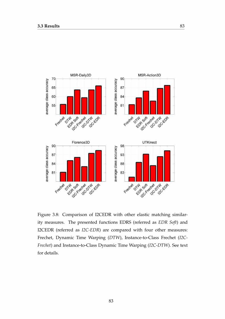
3.3 Results 83
Figure 3.8: Comparison of I2CEDR with other elastic matching similar-
ity measures. The presented functions EDRS (referred as EDR Soft) and
I2CEDR (referred as I2C-EDR) are compared with four other measures:
Frechet, Dynamic Time Warping (DTW), Instance-to-Class Frechet (I2C-
Frechet) and Instance-to-Class Dynamic Time Warping (I2C-DTW). See text
for details.
83

3.3 Results 84
It is worth noting that all the results correspond to the basic single-part
classification approach. For simplicity, the multi-part approach described in
Section 3.2.3 was no used for these experiments.
The results support the claim about the superiority of our method for ac-
tion classification with respect to methods using on other sequence distance
functions.
3.3.3 Robustness analysis
In this section we detail a number of experiments aimed at testing the ro-
bustness of the proposed action recognition method. First, we analyze the
effect of adding independent identically distributed white noise to the skele-
tons. Then, we study the impact of local temporal shifts in the sequences.
Our approach is compared with several other methods, based on dif-
ferent modelings of the temporal information. Besides the methods based
on distance functions over raw sequence representations considered in Sec-
tion 3.3.2 (Frechet, DTW, I2CFrechet and I2CDTW), two other approaches
are included in the comparison: Fourier Temporal Pyramids (FTP) from
[WLWY12b], and Hidden Markov Model (HMM) from [LN06]. See Section
2.1.1 for a description of the methods. In every case, the optimal parameters
for FTP and HMM were found by leave-one-actor-out cross-validation (see
Section 2.2 for a description of the technique) on the training actors.
Experiments were carried out for two datasets: MSRDailyActivity3D
and UTKinect. In both cases, we show the relative accuracy obtained by
each of the tested methods, which is defined as the ratio between the aver-
age class accuracy under the perturbed scenario and the average class accu-
racy under the non-perturbed scenario.
Robustness to noise
We evaluated the robustness of the proposed approach to noise, along with
that of several other methods. For this purpose, we corrupted the skeletons
by adding noise from a Gaussian distribution with mean zero and variance
one. We compute the relative accuracy of each method for different amounts
84

3.3 Results 85
(a) (b)
Figure 3.9: Relationship between the relative accuracy and the noise stan-
dard variation for several methods on two datasets: MSRDailyActivity3D
(3.9a) and UTKinect (3.9b).
of noise, and studied the resulting behaviors.
Figure 3.9 shows the results for the two considered datasets. While, as
expected, relative accuracy decays with noise in every case, the degree in
which this happens varies depending on the method. Moreover, results on
MSRDailyActivity3D are generally worse than results on UTKinect, which
is reasonable considering that the former is a more challenging dataset.
Frechet exhibits the worst behavior in terms of robustness. The negative
effects of the maximum measure employed by this distance are evidenced
once again. Its I2C version (I2CFrechet) achieves some improvement on the
MSRDailyActivity3D dataset, although it shows less robustness than most
of the other methods. Hidden Markov Model results almost as sensitive
to noise as Frechet, presumably because of the instability of the procedure
used by HMM to compute the hidden states. DTW and EDR (indicated as
EDR Hard in the figure) offer similar robustness, suggesting that the quan-
tization of point distances is not, by itself, enough to make of EDR a more
robust measure than DTW. On the other hand, the incorporation of the soft
matching mechanism seems to give EDR the edge over DTW in terms of ro-
bustness, as EDRS shows larger relative accuracy than DTW for most of the
scenarios. Fourier Temporal Pyramid, I2CDTW and I2CEDR stand out as
85

3.3 Results 86
(a) (b)
Figure 3.10: Relationship between the relative accuracy and the temporal
misalignment for several methods on two datasets: MSRDailyActivity3D
(3.10a) and UTKinect (3.10b).
the most robust methods according to the tests. Dropping the Fourier coef-
ficients associated to high frequency components makes Fourier Temporal
Pyramid highly resilient to noise. The increased robustness of I2CDTW and
I2CEDR with respect to its I2I versions comes presumably from their ability
to match points from different sequences within a sequence set, thus miti-
gating the effects of noisy points.
Robustness to temporal misalignment
To test the robustness of our method to temporal misalignment, we circu-
larly shifted every skeleton descriptor sequence in the training data. The
(uncorrupted) testing data was classified by a given method several times,
each corresponding to a different number of shifted frames. Again, we com-
pare the relative accuracy of our approach with that of the other methods.
Figure 3.10 shows the results for the two datasets. Accuracy deterio-
rates for most of the methods as the number of shifted frames increases.
The exception is HMM, which achieves almost the same accuracy for every
scenario. This was expected as it is well known that HMM performance
does not depend on the sequences being aligned. A variety of behaviors is
observed for the rest of the methods.
86

3.3 Results 87
Frechet once again gives the worst results on both datasets. This can also
be attributed to the instability caused by the maximum computation. DTW,
EDR, and EDRS show roughly the same robustness. This makes sense, as
the main difference between the three methods does not lie in the ability to
deal with time shifting. A similar reasoning can be used to explain the be-
havior of I2CEDR and I2CDTW. While achieving slightly better results than
their I2I versions for 15 and 20 shifted frames, they show nearly the same
robustness than those methods in most of the scenarios. FTP shows consid-
erable robustness in every case, thanks to its usage of the frequency domain.
Overall, we see that the proposed I2CEDR shows considerable tolerance to
temporal misalignment and stands out as one of the more robust methods
among the compared approaches.
3.3.4 Comparison with the state-of-the-art
In this section, we compare the results obtained by our proposed action
recognition approach with those of several state-of-the-art methods. In or-
der to make a fair comparison, we only consider those works focusing on
skeleton-based action classification. That is, we do not include results cor-
responding to methods employing depth or RGB information.
Table 3.1 shows the average class accuracy of each method for the four
considered datasets. In comparison to the state-of-the-art our method is able
to be on par with previously reported results, achieving competitive perfor-
mance on the four datasets. On the Florence3D dataset, it even outperforms
the best accuracy known to us (85.20%) by 4.30%. On the rest of the datasets,
it is among the top performing approaches.
It is worth mentioning that many of the methods referenced in Table 3.1
( [CPLFR13, YT12, XCA12, ATSS15, SVB+13]) use skeleton descriptors dif-
ferent to the RJP (described in Section 3.2.3) employed in our approach, as
well as different preprocessing techniques. For example, [CPLFR13] consid-
ers a descriptor that extends RJP with joint offset and velocity information,
[YT12] further improves that descriptor by applying Principal Component
Analysis (PCA), [XCA12] uses histograms of joints positions, and [SVB+13]
87

3.3 Results 88
MSRDailyActivity3D dataset
Fourier Temporal Pyramid [WLWY12b] 68.00
Weakly-aligned Bag of Poses [SVB+13] 70.00
Proposed method 68.00
MSRAction3D dataset
Hidden Markov Model [XCA12] 78.97
Naive-Bayes-Nearest-Neighbor [YT12] 82.30
Joint Angle Similarities [OBT13] 83.53
Elastic Functional Coding [ATSS15] 85.16
Fourier Temporal Pyramid [WLWY12b] 88.20
DTW Nominal Curve + FTP [VAC14] 88.23
Bag of Temporal and Spatial Part-Sets [WWY13] 90.22
Random Forest [ZCG13] 90.90
Recurrent Neural Networks [DWW15] 94.49
Proposed method 88.42
UTKinect dataset
Random Forest [ZCG13] 87.90
Hidden Markov Model [XCA12] 90.92
Elastic Functional Coding [ATSS15] 94.87
DTW Nominal Curve + FTP [VAC14] 95.58
Proposed method 95.28
Florence3D dataset
Weakly-aligned Bag of Poses [SVB+13] 82.00
DTW Nominal Curve + FTP [VAC14] 85.20
Proposed method 89.50
Table 3.1: Comparison of the proposed approach with the state-of-the-art.
88

3.4 Resumen 89
models the human torso as a rigid part, expressing the position of the joints
in a coordinate system derived from the torso orientation. Therefore, Ta-
ble 3.1 should be approached with caution in terms of temporal modeling
comparison, as the differences in accuracies may be caused by several other
factors. Nevertheless, the table shows that the proposed method can yield
very satisfactory results, and encourages the use of the I2CEDR distance for
action recognition based on skeleton sequences.
3.4 Resumen
En este capıtulo se presenta el primero de los dos metodos propuestos en la
tesis para el reconocimiento de acciones en videos de profundidad. El mis-
mo esta basado en una nueva tecnica para comparar secuencias, obtenida
como resultado de dos modificaciones a una conocida medida de similari-
dad entre secuencias.
La seccion 3.1 presenta un repaso general a los enfoques elegidos por
trabajos anteriores para modelar la evolucion temporal de secuencias de es-
queletos. Dicho repaso analiza los principales defectos de los metodos des-
criptos y sirve como motivacion para presentar el enfoque propuesto en la
tesis.
La seccion 3.2 presenta la nueva tecnica para comparar secuencias y
el metodo de reconocimiento de acciones basado en ella. Primero (seccion
3.2.1), se repasan varias tecnicas clasicas para comparacion de secuencias,
poniendo especial enfasis en un grupo de tecnicas que calcula la distancia
entre secuencias buscando el mejor (de acuerdo a una determinada funcion
de costo) alineamiento posible entre los puntos de las secuencias compara-
das. Entre ellas se encuentra la medida conocida como Edit Distance on Real
sequence (EDR), que tiende a ser mas precisa y mas robusta al ruido que otras
tecnicas del grupo. La seccion 3.2.2 introduce la tecnica propuesta en la te-
sis, obtenida mediante dos modificaciones clave a EDR. La primera consiste
en la introduccion de una funcion de costo suave para el alineamiento de
puntos, que apunta a hacer de EDR una medida mas precisa, permitiendo
caracterizar diferencias mas sutiles entre los puntos alineados. La segunda
89

3.4 Resumen 90
modificacion incorpora la nocion de distancia Instancia-a-Clase (I2C, por el
termino en ingles Instance-to-Class) a EDR, y permite alinear puntos de la
secuencia a clasificar con puntos pertenecientes a distintas secuencias, me-
jorando la capacidad de generalizacion de clasificadores no-parametricos
en casos de alta variabilidad intra-clase y pocos datos de entrenamiento.
Al ser derivada a partir de EDR, la tecnica propuesta tiene especialmente
el ordenamiento temporal a la hora de alinear puntos. Como un beneficio
adicional, no requiere aprendizaje de parametros. La seccion 3.2.3 describe
el metodo propuesto para reconocimiento de acciones basado en secuencias
de esqueleto. El metodo clasifica una secuencia dada basandose en la simi-
laridad de la misma con varios conjuntos de secuencias de entrenamiento.
Dicha similaridad es medida utilizando la tecnica propuesta en la seccion
3.2.2. La seccion detalla el modo exacto en que la tecnica es usada, ası como
varios preprocesamientos aplicados a las secuencias originales de esquele-
tos antes de la clasificacion.
La seccion 3.3 presenta los resultados de los experimentos realizados con
el metodo propuesto en cuatro bases de datos. En particular, se evaluan las
mejoras obtenidas respecto de metodos basados en EDR y en otras medidas
de alineamiento de secuencias. Ademas, se evalua la robustez del metodo
respecto al ruido y al desfasaje temporal. Por ultimo, se compara el rendi-
miento del mismo con el estado del arte.
90

Chapter 4
Action recognition using
Citation-kNN on bags of
time-stamped poses
This chapter describes the second novel method for action recognition pre-
sented in the thesis. Its main feature is a new Multiple Instance Learning
(MIL) approach to the problem. Section 4.1 explains the reasoning behind
the MIL approach. Section 4.2 reviews MIL concepts needed to understand
our proposal and presents the action recognition method. Finally, Section
4.3 experimentally evaluates our method and compares it with the state-of-
the-art.
4.1 Introduction
As discussed in Section 1.1.1, modeling the temporal evolution of skele-
ton descriptors is a challenging task, due mainly to the noisy joints, and
the inherently large intra-class variability/inter-class similarity (in skeleton
spatial configurations as well as in execution speed and temporal misalign-
ment). This challenges have been addressed in a variety of ways in previous
works. Sections 1.1.1 and 3.1 detail many of the existent approaches to the
problem.
Most of those approaches attempt to capture the main features of the

4.1 Introduction 92
temporal evolution in a single representation, either by training a model or
classifier specifically suited for time series, by using distance functions ap-
propriate for temporal patterns, or by computing a high level description of
the temporal sequence based on the individual skeletons. In doing so, they
face the challenges commented above. The proposed representation has to
be general enough as to abstract away the inherent intra-class variability
and the noisy skeletons, and, at the same time, it has to be able to discrimi-
nate between very similar sequences corresponding to different actions. The
proposed solutions are typically sophisticated, highly hand-crafted and re-
quire a lot of tuning.
In contrast, we explicitly acknowledge that the number of discrimina-
tive skeletons in a sequence might be low. The rest of the skeletons might
be noisy, correspond to subject-specific poses, occur at uncommon frames,
or have a configuration common to several actions (for example, a sit still
configuration). In other words, we know that certain actor poses, when oc-
curring at specific times, provide discriminative information about the per-
formed action. But we do not know exactly which poses (in terms of con-
figuration and time location) those are. At the same time, many other poses
may provide no information, or may even be misleading or ambiguous.
Thus, the problem can be naturally treated as a Multiple Instance Learn-
ing (MIL) problem. In MIL, training instances are organized into bags. A
bag from a given class contains some instances that are characteristic of that
class, but might (and most probably will) contain instances that are not. Fol-
lowing this idea, we represent videos as bags of time-stamped skeleton de-
scriptors, and we propose a new framework based on Citation-kNN [WZ00]
for action recognition.
Approaching the task using a MIL framework allows our method to con-
dense all the descriptors in a loose representation to decide the sequence
class. As long as a few representative descriptors occur at the right time, the
query video has a good chance of being correctly classified. We found that
our approach is effective in dealing with the large intra-class variability/inter-
class similarity nature of the problem. The proposed framework is simple
and provides a clear way or regulating tolerance to noise and temporal mis-
92

4.2 Recognizing actions with Citation-kNN on bags of time-stampedposes 93
alignment.
To the best of our knowledge we are the first to use Citation-kNN for
this problem. MIL has been considered before [YHC+12] for skeleton-based
action recognition. However, their main reason for using a MIL approach
is the presence of irrelevant actions in the videos as a consequence of inac-
curate manual segmentation. Furthermore, their goal is the classification of
actions involving two people. On the other hand, we aim at exploring the
MIL ability to deal with the large intra-class variability/inter-class similar-
ity of the single-person action recognition problem.
Experimental results support the validity of the proposed approach. Ex-
tensive tests on four datasets verify the robustness of our method and show
that it compares favorably to other state-of-the-art action recognition meth-
ods.
4.2 Recognizing actions with Citation-kNN on bags
of time-stamped poses
This section describes the Multiple Instance Learning (MIL) approach pro-
posed for skeleton-based action recognition. Sections 4.2.1 and 4.2.2 review
MIL and Citation-kNN, the specific MIL method used by our approach. Sec-
tion 4.2.3 presents a modified version of Citation-kNN. Finally, Section 4.2.4
presents our method for action recognition based on Citation-kNN.
4.2.1 Multiple Instance Learning
Multiple Instance Learning (MIL) is a variant of supervised machine learn-
ing in which the training examples come in the form of bags. A bag is a set
of feature vectors, called instances. Each training bag has, as in traditional
supervised learning, an assigned class label. The goal is to learn a model
capable of predicting class labels for unseen query bags. Note how this
setting considerably differs from classical single instance supervised learn-
ing, in which training data is organized as individual feature vectors, and
a class label is available for each vector. Following the usual procedure in
93
4.2 Recognizing actions with Citation-kNN on bags of time-stampedposes 94
the literature, we present MIL as a binary classification task. Multiple-class
classification can be obtained following typical one-vs-one or one-vs-rest
strategies [Bis06], although other approaches are possible (see for example
our proposed method in Section 4.2.4).
More formally, a bag is defined as a set of instances X = {x1, . . . , xM}
where each of the instances xi is a vector in a d-dimensional space, i.e. xi ∈
Rd ∀ 1 ≤ i ≤ M. The goal in MIL is to learn a classification function
C(X) ∈ [0, 1] that predicts 1 if and only if X is estimated to be positive. The
training set T = {(X1, y1), . . . , (XN, yN)} consists of N bags and its labels.
For each bag Xi, its label yi ∈ {0, 1} indicates whether Xi is positive (yi = 1)
or negative (yi = 0).
A variety of approaches to the MIL task have been proposed over the
years [DLLP97, MLP98, WFP03, ZG01, ATH02, ZX07, CBW06, Don06]. Every
method relies on a specific assumption about the relationship between a
bag label and the instances within that bag. Early works [DLLP97, MLP98]
assume that every instance has an assigned hidden label, and that every
bag with a positive label contains at least one positive instance. Further,
negative bags do not contain any positive instances. This assumption is
known as the standard MI assumption. A considerable part of the most recent
works [WFP03, SZB05, CBW06, Don06], however, relaxes this assumption.
In particular, the approach used in this work (see Section 4.2.2) is based on
the very loose assumption that bags that are similar according to a given
distance measure are likely to have the same class label. The key aspect of
the approach is, of course, the distance measure considered for comparing
bags.
4.2.2 Citation-kNN
Citation-kNN is presented in [WZ00] as a way of adapting the k-Nearest
Neighbors (kNN) approach to the multiple instance task. In the single in-
stance variant of kNN, traditional distance functions such as Lp norms can
be used to compare examples. In MIL though, proper distance functions be-
tween bags have to be used instead. Moreover, the usual kNN method for
94

4.2 Recognizing actions with Citation-kNN on bags of time-stampedposes 95
selecting the label of a query example based on the majority class of the clos-
est neighbors may not lead to good classification results. Therefore, other
ways of combining the labels of the nearest bags have to be considered.
The chosen distance function in Citation-kNN is a modified version of
the Hausdorff distance. Given two set of points A = {a1, . . . , aM} and B =
{b1, . . . , bN}, the Hausdorff distance is defined as:
H(A, B) = max(h(A, B), h(B, A)) (4.1)
where
h(A, B) = maxa∈A
minb∈B‖a− b‖ (4.2)
and ‖ · ‖ is a norm on the points of A and B.
The function h(A, B) is known as the directed Hausdorff distance from A
to B. If we denote by a the point in A that is farthest from any point in B,
then h(A, B) is the distance from a to its nearest neighbor in B. Note that if
h(A, B) = d, then each point of A is within distance d of at least one point
in B and, further, there is some point in A that is exactly at distance d from
its nearest neighbor in B. For future reference, we call A the source set and B
the target set.
The Hausdorff distance measures the degree in which the compared sets
A and B differ from one another. It does it by measuring the distance of the
point in A that is farthest from any point in B and vice versa. A Hausdorff
distance of d indicates that every point in A is within distance d from some
point in B, and that every point in B is within distance d from some point
in A. Therefore, two sets are similar if each point in one set is close to some
point in the other set, and vice versa.
A small Hausdorff distance is obtained if and only if every point of one
set is near some point of the other set. Thus, a single outlier can severely
distort the distance. In order to increase its robustness with respect to out-
liers, a modified version of the distance is used in [WZ00]. The modified
measure considers a different function for the directed Hausdorff distance
from A to B, h(A, B). Specifically, each point in A is ranked by the distance to
its nearest point in B, and the R-th ranked such point determines the modi-
95

4.2 Recognizing actions with Citation-kNN on bags of time-stampedposes 96
fied distance. Formally, if M is the number of points in A and 1 ≤ S ≤ M,
hS(A, B) is defined as:
hS(A, B) = Sth
a∈Aminb∈B‖a− b‖, (4.3)
where Sth
a∈Ais the S-th ranked distance in the set of distances (one for each
element in A).
The value of S is usually defined indirectly by specifying a fraction 0 ≤
K ≤ 1 of the points in A. Therefore, after ranking each of the M points in
A by the distance to its nearest point in B, the value corresponding to po-
sition S = max(⌊KM⌋ , 1) of the ranking is the modified directed distance.
Note that when K = 1, the largest distance in the ranking is used, and thus
hS(A, B) is the same as h(A, B). On the other hand, when K ≤ 1M , the mini-
mal of the M point distances decides the modified directed distance.
The modified Hausdorff distance is given by:
HSL(A, B) = max(hS(A, B), hL(B, A)) (4.4)
where S and L indicate the considered number of points from A and B re-
spectively.
Again, S and L are usually determined using a single K value. Specif-
ically, if M is the number of points in A and N is the number of points in
B, then S = max(⌊KM⌋ , 1) and L = max(⌊KN⌋ , 1). Setting K = 1 results
in S = M and L = N (i.e. the standard Citation-kNN), while setting K to a
value such that K ≤ 1M and K ≤ 1
N results in S = L = 1. This last variant is
typically called minimal Hausdorff distance.
In [WZ00], the conventional kNN procedure for selecting the label of a
query example was found not to be optimal for the MIL scenario. In their
experiments with binary classification, the authors observed that negative
examples might frequently contain more positive bags than negative bags
among their nearest neighbors. Thus, predicting an example label based on
the majority class of the closest neighbors will generally yield low accuracy.
This phenomena might be due to the presence of false positive instances in
the positive bags, that may attract negative bags. This situation is explained
96
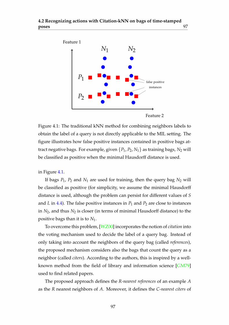
4.2 Recognizing actions with Citation-kNN on bags of time-stampedposes 97
P1
P2
N1 N2
false positive
instances
Feature 2
Feature 1
Figure 4.1: The traditional kNN method for combining neighbors labels to
obtain the label of a query is not directly applicable to the MIL setting. The
figure illustrates how false positive instances contained in positive bags at-
tract negative bags. For example, given {P1, P2, N1} as training bags, N2 will
be classified as positive when the minimal Hausdorff distance is used.
in Figure 4.1.
If bags P1, P2 and N1 are used for training, then the query bag N2 will
be classified as positive (for simplicity, we assume the minimal Hausdorff
distance is used, although the problem can persist for different values of S
and L in 4.4). The false positive instances in P1 and P2 are close to instances
in N2, and thus N2 is closer (in terms of minimal Hausdorff distance) to the
positive bags than it is to N1.
To overcome this problem, [WZ00] incorporates the notion of citation into
the voting mechanism used to decide the label of a query bag. Instead of
only taking into account the neighbors of the query bag (called references),
the proposed mechanism considers also the bags that count the query as a
neighbor (called citers). According to the authors, this is inspired by a well-
known method from the field of library and information science [GM79]
used to find related papers.
The proposed approach defines the R-nearest references of an example A
as the R nearest neighbors of A. Moreover, it defines the C-nearest citers of
97

4.2 Recognizing actions with Citation-kNN on bags of time-stampedposes 98
A to be the set that includes any given bag X if and only if A is one of the C
nearest neighbors of X. Note that, in general, the number of C-nearest citers
is not C.
The class of a query bag is derived by combining the votes of its R-
nearest references with those of its C-nearest citers. For binary classifica-
tion, the number of positive votes p is determined by summing the number
of positive references Rp and positive citers Cp, i.e. p = Rp + Cp. Likewise,
if the number of positive and negative references are Rn and Cn respectively,
the number of negative votes is n = Rn + Cn. The query is predicted posi-
tive if p > n, and negative otherwise.
4.2.3 Modified Citation-kNN
This section presents a modified version of Citation-kNN, which introduces
two changes to the original method. First, it extends it to allow for multiple-
class classification. Second, it adjusts the voting mechanism by incorporat-
ing weighted votes. Both changes are a natural application of ideas com-
monly used in the kNN method.
The voting procedure described in Section 4.2.2 was thought for binary
classification. Like other binary methods, this procedure can be combined
with (for example) a one-vs-one or one-vs-rest strategy to allow for multiple-
class classification. However, a more natural extension to the multiple class
scenario can be devised for Citation-kNN. We now present such extension.
Let L be the set of possible labels. For a given query bag X, assume
{r1, . . . , rnr} and {c1, . . . , cnc} are the class labels of its nr nearest references
and its nc nearest citers respectively. In our extension, the predicted label l∗
for X is obtained by summing the votes of citers and references as:
l∗ = arg maxl∈L
(nc
∑i=1
δ(l, ci) +nr
∑j=1
δ(l, rj)) (4.5)
where δ(a, b) = 1 if a = b and δ(a, b) = 0 otherwise.
The criteria presented in Equation 4.5 assigns the same importance to the
vote of any citer or reference. However, it seems reasonable to pay more at-
tention to those neighbors that are closer to the query bag. In other words,
98

4.2 Recognizing actions with Citation-kNN on bags of time-stampedposes 99
examples that are closer to the query should count for more. This can be
achieved by using weighted voting. Formally, let X be the query example,
L be the set of possible labels, and assume {R1, . . . , Rnr} and {C1, . . . , Cnc}
are the sets of nearest references and citers of X respectively. Further, let
{r1, . . . , rnr} and {c1, . . . , cnc} be the class labels of its nearest references and
its nearest citers respectively. Then, the weighted voting approach for pre-
dicting label l∗ for X is:
l∗ = arg maxl∈L
(nc
∑i=1
αiδ(l, ci) +nr
∑i=1
βiδ(l, ri)) (4.6)
where αi is the weight for citer Ci and βi is the weight for reference Ri.
Clearly, the weight for a particular example should be a decreasing func-
tion of its distance to X. In this work we use the following popular choice
for kNN:
αi =1
H(X, Ci)βi =
1
H(X, Ri)(4.7)
where H(·) is the modified Hausdorff distance described in Equation 4.4
(we omit the S and L subscripts here for clarity).
Note that the weight functions in Equation 4.7 are not defined when the
distance between the compared examples is zero. Therefore, when a neigh-
bour matches the query exactly, we directly assign l∗ to be the label of such
neighbour.
4.2.4 Citation-kNN on bags of time-stamped poses
This section describes the proposed method for action recognition based
on Citation-kNN. As explained in Chapter 1.2, the raw representation of
an action execution is given by a sequence of skeletons, that encodes the
temporal evolution of the actor’s pose (see Section 3.2.3 for details).
In this method, skeletons are normalized using the same procedure as in
Section 3.2.3. Furthermore, the relative position of the joints (RJP), detailed
in Section 3.2.3 is used as skeleton descriptor.
99

4.2 Recognizing actions with Citation-kNN on bags of time-stampedposes 100
In the following, we introduce the specific representation for descriptor
sequences used by the presented method, and we study the application of
Hausdorff distance on such representation. Then, we describe the classifi-
cation procedure for new skeleton sequences.
Representing skeleton descriptor sequences as bags of time-stamped skele-
ton descriptors
Any given skeleton descriptor sequence contains descriptors that are repre-
sentative of the action being performed. However, at the same time, many
other descriptors in the sequence provide no information (or worse, they
are misleading) about the action label. As explained in sections 1.1.1 and
4.1, this is due not only to the nature of action sequences (which have large
inherent inter-class similarity and intra-class variability), but also to the
high degree of noise and outliers present in sequences captured with typical
depth devices.
Formally, given a sequence X = (x1, x2, . . . , xN) with N skeleton descrip-
tors, its time-stamped bag representation is the set BX = {b1, b2, . . . , bN},
where bi = (xi, α iN ) is the ordered pair obtained by appending a single
value to descriptor xi. The appended value α iN adds temporal information
to the original descriptor. It is computed by multiplying the relative tempo-
ral position of the descriptor (i.e. the video frame at which the descriptors
is located divided by the total number of frames in the video) by a constant
α, that regulates the weight of the temporal information. We refer to α as
the frame weight and to bi as a time-stamped descriptor. Bags of time-stamped
descriptors are compared using the modified Hausdorff distance given in
Equation 4.4. We now present a series of examples that aim at gaining fur-
ther insight into the proposed bag representation and the chosen distance
function.
Comparing bags of skeletons descriptors using the Hausdorff distance
Figure 4.2 illustrates how the Hausdorff distance between two bags of de-
scriptors is obtained. The compared bags correspond to the actions cheer
100

4.2 Recognizing actions with Citation-kNN on bags of time-stampedposes 101
up and drink. For clarity purposes, the original sequences (belonging to
the dataset MSRDailyActivity3D described in Section 2.2) were brought to
a length of only 6 frames.
Figure 4.2a shows the distance between each descriptor in the cheer up
bag and its nearest neighbor in the drink bag. I.e., it shows the values in-
volved in the computation of the directed Hausdorff distance (Equation 4.2)
from the cheer up bag to the drink bag. Figure 4.2b illustrates in turn the di-
rected Hausdorff distance from the drink bag to the cheer up bag. In both
figures, descriptors are linked to their nearest neighbor by an arrow. Note
how multiple descriptors from one set can be map to the same descriptor
in the other set. Arrows are colored according to the color scale shown on
the right. Arrow color serves as an additional indication of the distance be-
tween the linked descriptors. Observe that each descriptor is represented by
its corresponding skeleton (that is, the skeleton from which it was obtained).
Moreover, skeletons are shown in the order they appear in the original se-
quence. In this example, frame information was not considered. That is, a
frame weight α = 0 was used.
For both figures 4.2a and 4.2b, it can be seen that descriptors correspond-
ing to neutral poses (located roughly at the beginning and at the end of the
sequences) are relatively close to their nearest neighbors. This is expected
behavior, since the neutral pose is common to both actions. On the other
hand, the more representative poses of each action (both hands above the
head in the case of cheer up and one hand next to the head in the case of
dink) lead to larger distances. The largest distances are produced by the most
characteristic poses of the cheer up sequence. In particular, one of those dis-
tances (91.13) determines the final Hausdorff distance when K = 1 is used.
This example illustrates an important assumption of our approach: Even
though two differently labeled action sequences may (and most probably
will) contain many similar poses, at least one of the sequences will contain
poses that differentiate it from the other sequence. Therefore, when com-
paring the bag representations of those sequences, descriptors originated in
such differentiating poses will be at large distance from their nearest neigh-
bors in the other bag. As a consequence, the Hausdorff distance will be
101

4.2 Recognizing actions with Citation-kNN on bags of time-stampedposes 102
large. On the contrary, two sequences with the same label will share most
of their poses, causing the Hausdorff distance between their corresponding
bags to be small.
Taking temporal information into account
In the example of Figure 4.2 time was not taken into account. While this
may not be a problem for some actions, ignoring temporal information can
severely hurt classification performance in other cases. This is illustrated in
figures 4.3a and 4.3b. The figures show the comparison of a query sit down
bag with two other bags: another sit down bag and stand up bag. A frame
weight α = 0 was used. For future reference, we call the bags Q, A and
B respectively. Specifically, Figure 4.3a illustrates the directed Hausdorff
distance from the A to Q, h(A, Q), while Figure 4.3a illustrates the directed
Hausdorff distance from the B to Q, h(B, Q). For clarity, only one direction
of the Hausdorff distance is shown for each comparison. Take into account,
however, that considering both directions is important for achieving good
results.
Clearly, it is desirable that h(B, Q) < h(A, Q), because Q and B are la-
beled with the same action, and Q and A are not. However, as both ac-
tions sit down and stand up involve similar poses, h(A, Q) is smaller than
desired. In general, sit down bags contain skeleton descriptors that are simi-
lar to the ones found in stand up bags, namely those corresponding to siting
and standing poses. As a consequence, every descriptor in one bag has a
close nearest neighbor in the other bag, yielding a small distance between
bags. In this example, even though the distances involved in the compu-
tation of h(B, Q) are also small, a few of them are slightly larger than the
ones involved in the computation of h(A, Q), causing h(B, Q) > h(A, Q).
The unexpected behavior came from discarding temporal information. The
compared actions can be easily confused if the temporal order is not taken
into account.
The effect of choosing an adequate value for the frame weight is illus-
trated in Figure 4.4. The figure shows the same comparisons described in
Figure 4.3. In this case, however, time information is taken into account.
102

4.2 Recognizing actions with Citation-kNN on bags of time-stampedposes 103
(a)
(b)
Figure 4.2: Illustration of the Hausdorff distance between two bags of skele-
ton descriptors, corresponding to the actions cheer up and drink. Figure 4.2a
describes the directed Hausdorff distance from the cheer up bag to the drink
bag. Figure 4.2b describes the distances for the directed Hausdorff distance
from the drink bag to the cheer up bag. Each descriptor in the source bag is
linked by an arrow to its nearest neighbor in the target bag. The distance
to such nearest neighbor is indicated both by the color of the arrow (follow-
ing the color scale shown on the right side) and by the number next to the
arrow. See text for details.
103

4.2 Recognizing actions with Citation-kNN on bags of time-stampedposes 104
(a)
(b)
Figure 4.3: Illustration of the Hausdorff distance between a query bag and
two training bags of skeleton descriptors. The query bag corresponds to
the action sit down. Training bags are labeled with the actions sit down and
stand up. Figure 4.3a describes the directed Hausdorff distance from the
stand up bag to the query bag. Figure 4.3b describes the directed Hausdorff
distance from the sit down training bag to the query bag. Temporal order is
not considered. Descriptors in the source bag are linked by an arrow to their
nearest neighbors in the target bag. The distance to such nearest neighbor
is indicated both by the color of the arrow (following the color scale shown
on the right side) and by the number next to the arrow. See text for details.
104

4.2 Recognizing actions with Citation-kNN on bags of time-stampedposes 105
Note how the temporal information forces each descriptor to be linked to a
descriptor located at a similar temporal position. This has particularly ben-
eficial effects on the comparison between the sit down and the stand up bags,
shown in Figure 4.4a. For example, the rightmost descriptor in the bottom
row (corresponding to the standing pose) cannot longer be (costless) linked
to a descriptor located in left-half of the top row (as it happens in Figure
4.3a). In other words, it is forced to find its nearest neighbor among de-
scriptors with which is not similar in terms of pose. Compared to example
in Figure 4.3a, the computation of the Hausdorff distance between sit down
bag and the stand up bag involves larger values, causing bags to be further
apart. On the other hand, the Hausdorff distance between the two sit down
bags does not change significantly, because similar poses are located at sim-
ilar temporal locations in the original sequences. The ultimate consequence
is that the query bag is closer to the sit down bag than the stand up bag, as
desired.
The effect of the K parameter
Recall from Section 4.2.2 that the modified Hausdorff distance can be tuned
by specifying the parameter 0 ≤ K ≤ 1. This parameter indicates the frac-
tion of the points that are to be considered to compute the similarity be-
tween the two bags. In other words, 1− K% of the points is ignored when
computing the modified Hausdorff distance.
To illustrate the effect of the K parameter, Figure 4.5 compares a query
cheer up bag with two other bags. Specifically, Figure 4.5a compares the
query with another cheer up bag, and Figure 4.5b compares it with a drink
bag. As in the example of the previous section, we use the names Q, A and
B for the considered bags, where Q is the query, A is the other cheer up bag
and B is the drink bag. In each figure, the values involved in the compu-
tation of the modified Hausdorff distance (Equation 4.4) are shown. Note
that, for clarity purposes, only one direction of the modified Hausdorff dis-
tanceis shown for each comparison. More precisely, Figure 4.5a illustrates
hS(A, Q), while Figure 4.5b illustrates hS(Q, A). We intentionally choose the
directions that produce the larger final distance in each case. Recall from
105

4.2 Recognizing actions with Citation-kNN on bags of time-stampedposes 106
(a)
(b)
Figure 4.4: Illustration of the Hausdorff distance between a query bag and
two training bags of skeleton descriptors. The compared bags are the same
as in Figure 4.3. Different from the scenario illustrated in that Figure, the
example shown here takes into account temporal information. See text for
details.
106
4.2 Recognizing actions with Citation-kNN on bags of time-stampedposes 107
Section 4.2.2 that the value of S is determined by K as S = max(⌊K6⌋ , 1).
It is desired that hL(A, Q) < hL(Q, B), since Q and A have the same la-
bel, while Q and B do not. However, a different result is obtained using
K = 1 (and thus L = 6). This is due to a very noisy skeleton in A. Specifi-
cally, the fourth skeleton from the right is severely perturbed by noise. As a
consequence, its associated descriptor lies far away from every descriptor in
Q, causing h6(A, Q) to be large. On the other hand, while h6(Q, B) involves
some large distances (as expected, because Q and B have different labels),
none of them is as large as the one associated with the noisy skeleton in A.
In the end, h6(A, Q) = 121.59 > h6(Q, B) = 55.67, which differs from the
expected result.
The desired behavior can be obtained, however, by letting K = 56 (and
thus L = 5). After ranking each of the 6 points in A by the distance to its
nearest point in Q, the value corresponding to position 5 of the ranking is
the modified directed distance from A to Q, h5(A, Q) = 33.91. Similarly, the
modified directed distance from Q to B is h5(Q, B) = 40.89. Note that, as
desired, h5(A, Q) < h5(Q, B).
It might seem that reducing K is always beneficial. However, note that
setting K = 36 (and thus L = 3) again gives the undesired result h3(A, Q) =
18.78 > h3(Q, B) = 13.68. The problem comes from the fact the three more
discriminative poses in Q (namely, those in which both hands are above the
head) are ignored in the computation of h3(Q, B).
The following important conclusion can be drawn about the role of the
K parameter based on the previous example. It is possible to make the dis-
tance robust against noisy and outlying descriptors by adjusting the value
of K. More precisely, if n% of the descriptors in a bag are known to be noise
or outliers, then using a value of K such that K < 1− n, leaves those de-
scriptors out of the computations, avoiding their undesired effects on the
final distance. However, if the value of K is too low, then the descriptors
that differentiate one bag from the other might also be ignored. Specifically,
if the fraction of noisy and discriminative descriptors are known to be of n%
and d% respectively (assume, for simplicity, that the fractions are the same
for both bags), then setting K to a value less than 1− n− d discards not only
107

4.2 Recognizing actions with Citation-kNN on bags of time-stampedposes 108
(a)
(b)
Figure 4.5: Illustration of the Hausdorff distance between a query bag and
two training bags of skeleton descriptors. The query bag corresponds to the
action cheer up. Training bags are labeled with the actions cheer up and drink.
Figure 4.5a describes the directed Hausdorff distance from the cheer up bag
to the query bag. Figure 4.5b describes the directed Hausdorff distance from
the query bag to the cheer up training bag. One of the descriptors in the cheer
up training bag is very noisy. Descriptors in the source bag are linked by
an arrow to their nearest neighbors in the target bag. The distance to such
nearest neighbor is indicated both by the color of the arrow (following the
color scale shown on the right side) and by the number next to the arrow.
See text for details. 108

4.2 Recognizing actions with Citation-kNN on bags of time-stampedposes 109
the noisy descriptors but also the informative ones. Thus, the optimal K
must lie at some point between 1− n and 1− n− d. Of course, n and d vary
depending on the bags, and are generally not known in advance. Therefore,
the value of K has to be decided empirically.
Video classification procedure
This section presents an overview of the main steps involved in the clas-
sification of a query video. Recall from the beginning of this section and
from Chapter 1 that the raw representation of action sequence is given by
a sequence of skeletons. Therefore, our presented method attempts to pre-
dict the action label of a query skeleton sequence, based on labeled training
sequences.
After skeleton normalization and descriptor computation (see the begin-
ning of Section 4.2.4), the original sequences in the training data are trans-
formed into bags of time-stamped descriptors, as explained in Section4.2.4.
The same procedure is applied for a query sequence before classification.
Therefore, action prediction for a query sequence A consists of three steps:
1. Obtain a sequence of normalized skeletons by normalizing each skele-
ton in A,
2. Obtain a sequence of skeleton descriptors by computing a descriptor
for each skeleton normalized in the previous step,
3. Obtain a bag of time-stamped skeleton descriptors by appending tem-
poral information to each descriptor computed in the previous step,
4. Classify the bag of the time-stamped skeleton descriptors obtained in
the previous step.
Step 4 above predicts the label of the sequence A using the multi-class
distance-weighted classification approach presented in Section 4.2.3.
Multi-part approach
Similar to the method described in Section 3.2.3, we improve the basic clas-
sification step using a multi-part approach. Recall from equations 3.20 and
109

4.2 Recognizing actions with Citation-kNN on bags of time-stampedposes 110
3.21 that a skeleton descriptor is a 3(J− 1)J length vector d = (d1, d2, . . . , dJ),
where J is the number of joints in the skeleton and di is the 3(J − 1) length
vector corresponding to joint i. In addition, recall that when considering
time-stamped descriptors the value corresponding to the temporal informa-
tion is appended to the original descriptor. That is, if d is the ith descriptor
in a sequence with N elements, its associated time-stamped descriptor b is
a 3(J − 1)J + 1 length descriptor such that b = (d1, d2, . . . , dJ , α iN ).
For a given set p, we define a function fp that, given a skeleton descrip-
tor, it preserves the coordinates associated with joints in p and the tempo-
ral information, and discards the rest. Formally, if p = {p1, p2, . . . , pz} is
a set of z integers such that 1 ≤ pi ≤ J ∀ 1 ≤ i ≤ z, fp is a function
fp : R3(J−1)J+1 → R
3(J−1)z+1 such that:
fp((d1, d2, . . . , dJ , αi
N)) = (dp1
, dp2 , . . . , dpz , αi
N) (4.8)
We overload fp to describe a function that takes a bag of time-stamped
descriptors A = {a1, a2, . . . , aN} and applies fp to each of them:
fp(A) = { fp(a1), fp(a2), . . . , fp(aN)} (4.9)
Further, for a given set of time-stamped skeleton descriptors bags C =
{C1, C2, . . . , CK}, we overload fp as:
fp(C) = { fp(C1), fp(C2), . . . , fp(CK)} (4.10)
As in Section 3.2.3, we group joints into five body parts. For each part,
the problem stated in Equation 4.6 is solved. Formally, let A be the query
bag, L be the set of possible labels and T the set of all training bags. Assume
{Rp1 , . . . , R
p
npr} and {C
p1 , . . . , C
p
npc} are the sets of nearest references and citers
of fp(A) in fp(T), respectively. Further, let {rp1 , . . . , r
p
npr} and {c
p1 , . . . , cn
pc}
be the class labels of those references and citers respectively. We define
simpl (A), the similarity measure between fp(A) and class l, as:
simpl (A) =
npc
∑i=1
αpi δ(l, c
pi ) +
npr
∑i=1
βpi δ(l, r
pi ) (4.11)
110

4.3 Results 111
where δ(a, b) = 1 if a = b and δ(a, b) = 0 otherwise, and αpi and β
pi are
the weights for citer Cpi and reference R
pi respectively, determined using the
Hausdorff distance H(·) as:
αpi =
1
H( fp(A), Cpi )
βpi =
1
H( fp(A), Rpi )
(4.12)
Then, the multi-part approach for predicting label l∗ for A is:
l∗ = arg maxl∈L
∑p∈P
simpl (A)
Gp(A)(4.13)
where Gp(A) is a normalization factor, defined as:
Gp(A) = ∑l∈L
simpl (A) (4.14)
4.3 Results
This section presents and discuss experimental results for our proposed ac-
tion recognition method. As in Section 3.3, we use 4 different datasets: MSR-
DailyActivity3D, MSRAction3D, UTKinect and Florence3D. See section 2.2
for a thorough description of the datasets.
4.3.1 Parameter selection
Along Section 4.2, we describe several parameters that control the behavior
of the presented method. In order to select appropriate values for those pa-
rameters, we optimize the performance of our approach by cross-validation
on the training data. As the optimal parameters vary depending on the
dataset, we carry out such optimization procedure for each dataset.
The considered parameters are the frame weight α (see Section 4.2.4), the
K parameter for the modified Hausdorff distance (see Section 4.2.4), and the
values R and C that determine the number of references and citers of the
Citation-kNN method respectively.
A gradient ascent procedure is employed to obtain find optimal values for
the parameters. Specifically, such values are searched among the points of
111

4.3 Results 112
a grid that (roughly) divides the parameter space. Starting from a reason-
able point, the current point is updated at each iteration of the grid search.
More precisely, for each immediate neighbor of the current point, the av-
erage class accuracy for that point is computed using the leave-one-actor-
out cross-validation (LOAOCV) technique (see Section 2.2) on the training
data. After considering all the neighbors, the algorithm moves to the point
that produced the largest average class accuracy. Note that, as we have
four parameters to optimize, the grid is four-dimensional and the number
of neighbors for a grid point can be as large as 81. However, caching results
of previous points helps in reducing computation times. The grid search
finishes when no improvement is observed in the optimized measure. The
main reason for using this approach for parameter selection is its convenient
time complexity. In general, performing the gradient ascent is much faster
than evaluating every point in the grid. The price paid for the low temporal
complexity is that potentially optimal grid points might be not taken into
account.
4.3.2 Parameter influence
To evaluate the influence of the different parameters, we study the change
in performance obtained when varying one of them while leaving the rest
fixed. Specifically, the average class accuracy is computed using LOAOCV
on the training data for several values of the studied parameter. Such values
belong to a short range centered at the optimal value found by the grid
search described in Section 4.3.1. The remaining parameters are fixed at
their optimal values (also found by the grid search).
Figures 4.6a, 4.6b, 4.7a and 4.7b show the results for the MSRDailyActiv-
ity3D dataset, the MSRAction3D dataset, the UTKinect dataset and the Flo-
rence3D dataset respectively. In addition to the average class accuracy com-
puted by LOAOCV on the training data, the figures show the average class
accuracy computed on the test data (using the standard train-test regime for
each dataset, as described in Section 2.2). The former is denoted as train in
the figures, while the latter is denoted as test.
112

4.3 Results 113
(a) Parameter influence for the MSRDailyActivity3D dataset.
(b) Parameter influence for the MSRAction3D dataset.
Figure 4.6: Parameter influence for two of the four considered datasets.
Note that the influence of the parameters varies depending on the dataset.
113

4.3 Results 114
(a) Parameter influence for the UTKinect dataset.
(b) Parameter influence for the Florence3D dataset.
Figure 4.7: Parameter influence for two of the four considered datasets.
For example, the optimal K is around 0.55 for MSRDailyActivity3D, while
114

4.3 Results 115
it is around 0.88 for MSRAction3D. However, many behaviors common to
all datasets exist, as we discuss next.
In every considered dataset, performance drops somewhat drastically
when the frame weight is set below a specific threshold. Presumably, such
threshold corresponds to the point below which crucial temporal informa-
tion is discarded. Values above that threshold also lead to worse perfor-
mance. However, decrement is slower in this case, which suggests that giv-
ing excessive (but reasonable) importance to temporal order is less harmful
than ignoring it. It is worth commenting that, even if not shown in the plots,
an extremely large frame weight indeed shatters performance, as it allows
no temporal flexibility at all.
Figures also show a common pattern regarding the K parameter. Specif-
ically, high performance is achieved within a certain range, while low per-
formance is obtained outside the range. This is consistent with the obser-
vations in Section 4.2.4. Namely, that the optimal K must be low enough
as to leave noisy and outlying descriptors out of the computations, but
not as low as to ignore informative descriptors. Despite this common pat-
tern, note how the range varies for the different datasets. For example, it
is (roughly) [0.2, 0.76] for the UTKinect dataset and [0.66, 0.88] for the Flo-
rence3D dataset, which can be interpreted as the latter containing videos
with a smaller percentage of informative descriptors (indicated by the fact
that 0.88− 0.66 < 0, 76− 0.2) and a smaller percentage of noisy descriptors
(because 0.88 > 0.76).
In general, performance is not very sensitive to the number of refer-
ences and citers. While large deviations from the optimal values do cause a
change in accuracy, results show that such change tends to be smooth. This
is presumably due to the weighted voting mechanism explained in Section
4.2.3, that reduces the influence in the voting of those references and citers
located far away from the query bag.
115

4.3 Results 116
4.3.3 Evaluation of the main components of the action recog-
nition procedure
In this section, we experimentally study on two datasets (MSRDailyActiv-
ity3D and UTKinect) the impact on performance caused by the main com-
ponents of our method for action recognition. Specifically, we evaluate the
benefits of time-stamped descriptors (Section 4.2.4), weighted-voting (Sec-
tion 4.2.3) and the multi-part approach (Section 4.2.4).
We report results considering each component separately, but also for all
possible combinations of two and three components. Moreover, we include
results for basic variant of our method that does not use any of the compo-
nents. The basic version is indicated by Citation-kNN. Variants considering
only time-stamped descriptors, weighted voting or the multi-part approach
are indicated as Citation-kNN + time, Citation-kNN + weighted or Citation-kNN
+ parts respectively. Names for the solutions accounting for more than one
component together are indicated by combining the names of the single-
component variants. For example, Citation-kNN + time + weighted indicates
the combined use of time-stamped descriptors and weighted voting.
For each variant, the involved parameters were optimized using the gra-
dient ascent technique described in Section 4.3.1, and refined using the pro-
cedure explained in Section 4.3.2. Note that, depending on the variant,
different parameters need to be considered. For example, in the case of
Citation-kNN + parts + weighted, the frame weight parameter does not ex-
ist, because temporal information is not taken into account. The reported
measure is the average class accuracy computed on the test data (using the
standard train-test regime for each dataset, as described in Section 2.2).
Table 4.1 shows the results. In both datasets, performance of the ba-
sic Citation-kNN is considerably improved by the proposed method (i.e.
the variant than combines the three evaluated components). The table also
shows that every single-component variant yields better results than the ba-
sic approach. Further, it shows that the performance of any given variant
can be improved by extending it with any of its missing components.
Even though the exact relative benefit brought by each variant to the ba-
116

4.3 Results 117
sic approach depends on the dataset, improvements are consistent across
datasets for most of the variants. For example, the variant Citation-kNN +
parts + time yields an average class accuracy about 15% larger than the basic
approach on both datasets. However, two variants show particularly dif-
ferent behaviors in both datasets, in terms of the improvements to the basic
variant. The first one is Citation-kNN + weighted, that allows for an improve-
ment of 8% for the MSRDailyActivity3D dataset, but of only 1.7% for the
UTKinect. A possible explanation for this result could lie in the higher noise
levels of the MSRDailyActivity3D dataset (see Section 2.2). In that scenario,
it seems reasonable to find a relatively large number of misleading (i.e. la-
beled with a different action) neighbors among the citers and references of
the query bag. On the contrary, it is expect for such number to be low in a
less noisy scenario. Therefore, the benefit of weighting neighbors votes by
distance can be more noticeable in the noisy dataset.
The second variant that shows an interesting behavior is Citation-kNN +
time. For the UTKinect dataset, it allows for an improvement of aorund 12%
compared to the basic variant. However, such an improvement is of only 5%
for the MSRDailyActivity3D dataset. This suggests that using time-stamped
descriptors is more beneficial for the former dataset than it is for the latter.
Presumably, this is due to the fact that the relative number of actions for
which temporal order is decisive is lager in the UTKinect dataset. This ex-
planation is consistent with the frame weight plots in Figures 4.6a and 4.7a.
Those figures show that a quite large frame weight does not deteriorate per-
formance on the UTKinect dataset significantly, while small increments in
such weight cause a large decrease in performance on the MSRDailyActiv-
ity3D.
To further study the effects of time-stamped descriptors on performance,
we analyze the misclassified actions on both datasets when time informa-
tion is not taken into account. Figures 4.8a and 4.8b show confusion ma-
trices for the UTKinect dataset. The former corresponds to the the vari-
ant Citation-kNN + parts + weighted, that uses the multi-part approach and
weighted voting, but ignores temporal order. The latter corresponds to the
full method Citation-kNN + parts + weighted + time, that also take time into
117

4.3 Results 118
UTKinect MSRDaily
Citation-kNN 80.90 % 61.88 %
Citation-kNN + weighted 82.31 % 66.87 %
Citation-kNN + time 91.26 % 65.00 %
Citation-kNN + parts 85.02 % 66.87 %
Citation-kNN + weighted + time 92.36 % 69.37 %
Citation-kNN + parts + time 93.77 % 70.63 %
Citation-kNN + parts + weighted 86.94 % 68.13 %
Citation-kNN + parts + weighted + time 95.38 % 72.50 %
Table 4.1: Average class accuracy on datasets MSRDailyActivity3D and
UTKinect for different variants of the proposed method.
acount. Note how a considerable amount of error in Figure 4.8a comes from
confusing action sit down with action stand up, and action push with action
pull. The confused actions involve similar poses, meaning that any pose in
one of the actions can be found in the other action, and vice versa. The dif-
ferentiating aspect between those actions lies in the temporal location of the
poses. This is supported by Figure 4.8b, that shows a drastic reduction in
the confusion between them when using time-stamped descriptors.
Figures 4.9a and 4.9b show the confusion matrices corresponding to the
same variants for the MSRDailyActivity3D dataset. Note how the variant
that ignores temporal information confuses actions sit down and stand up.
Specifically, 60% of the videos labeled with one of the two actions is erro-
neously classified as corresponding to the other. When time is considered,
the confusion between them drops to 0%.
4.3.4 Robustness analysis
This section analyzes the tolerance of the proposed method to noise and
temporal misalignment. Similarly to Section 3.3.3, we study both the per-
formance in presence of independent identically distributed white noise in
the skeletons, and the impact of local temporal shifts on the descriptor se-
quences.
118

4.3 Results 119
(a) (b)
Figure 4.8: Confusion matrices for the UTKinect dataset. Figure 4.8a shows
the results obtained when time information is ignored. Figure 4.8b shows
the results obtained when taking temporal information into account.
Our approach is compared with two popular methods: Fourier Tempo-
ral Pyramids (FTP) from [WLWY12b], and Hidden Markov Model (HMM)
from [LN06]. See section 2.1.1 for a description of the methods. In every
case, the optimal parameters for FTP and HMM were found by leave-one-
actor-out cross-validation (see 2.2 for a description of the technique) on the
training actors. On the other, parameters for our method were optimized
using the gradient ascent technique described in Section 4.3.1, and refined
using the procedure explained in Section 4.3.2.
Experiments were carried out for two datasets: MSRDailyActivity3D
and UTKinect. In both cases, we show the relative accuracy obtained by
each of the tested methods, which is defined as the ratio between the aver-
age class accuracy under the perturbed scenario and the average class accu-
racy under the non-perturbed scenario.
Robustness to noise
We evaluated the noise robustness of the proposed approach, along with
that of several other methods. For this purpose, we corrupted the skeletons
by adding noise from a Gaussian distribution with mean zero and variance
119

4.3 Results 120
(a)
(b)
Figure 4.9: Confusion matrices for the MSRDailyActivity3D dataset. In Fig-
ure 4.9a time information is ignored, while in Figure 4.9b it is not.
120

4.3 Results 121
one. We compute the relative accuracy of each method for different amounts
of noise, and studied the resulting behaviors.
Figure 4.10 shows the results for the two considered datasets. While, as
expected, relative accuracy decays with noise in every case, the degree in
which this happens varies depending on the method. Moreover, results on
MSRDailyActivity3D are generally worse than results on UTKinect, which
is reasonable considering that the former is a more challenging dataset.
HMM shows the least robustness on both datasets. This is somewhat
expected, since it is well known that the procedure used by this method to
compute the hidden states is quite sensitive to noise. Our method and FTP
show a similar behavior. While the proposed approach seems to slightly
outperform FTP in terms of robustness on the MSRDailyActivity3D, both
methods obtain almost the same relative accuracy for most of the scenar-
ios on the UTKinect. As commented in 2.1.1, dropping the Fourier coeffi-
cients associated to high frequency components makes FTP highly resilient
to noise. Encouragingly, our method achieves similar robustness. We ar-
gue that a possible explanation lies mainly in two aspects of the proposed
multiple instance learning approach. First, the skeletons more affected by
noise can be ignored by the modified Hausdorff distance, as described in
Section 4.2.4. Second, the citation approach (improved by the weighted vot-
ing mechanism presented in Section 4.2.3) mitigates the effect of misleading
neighbors (potentially increased by noise).
Robustness to temporal misalignment
We compared the tolerance to temporal misalignment of the same methods
considered in Section 4.3.4. To that aim, we circularly shifted every skeleton
sequence in the training data, and kept the testing data uncorrupted. The
relative accuracy of our approach and that of FTP and HMM was computed
for several scenarios, each corresponding to a different number of shifted
frames.
Results for the two considered datasets are shown in Figure 4.11. It
is well known that the performance of HMM is not affected by sequence
alignment. This is reflected in its relative accuracy, that remains close to
121

4.3 Results 122
(a) (b)
Figure 4.10: Relationship between the relative accuracy and the noise stan-
dard variation for several methods on two datasets: MSRDailyActivity3D
(4.10a) and UTKinect (4.10b).
100% for every scenario on both datasets. Our method shows a robustness
comparable to that of FTP. Indeed, despite a somewhat erratic behavior, it
clearly outperforms such method on the MSRDailyActivity3D dataset. On
the other hand, both methods show very similar performance on UTKinect
dataset.
This test suggests that our method is more sensitive to temporal shifts
than HMM. Nevertheless, it shows competitive robustness, retaining a large
percentage of the average class accuracy obtained in the non-perturbed sce-
nario. This is presumably due to the same aspects commented in Section
4.3.4 for the noise experiments. Namely, the benefits brought by both the
Hausdorff distance and the citation approach with weighted voting. The
former reduces the effect of those skeletons shifted to unusual temporal po-
sitions. Such skeletons lead to misleading time-stamped descriptors, than
can be seen as noisy instances in the bag representation. The latter offers re-
silience against a potentially larger number of misleading neighbors, caused
by the larger presence of misleading time-stamped descriptors in the bags.
122

4.3 Results 123
(a) (b)
Figure 4.11: Relationship between the relative accuracy and the temporal
misalignment for several methods on two datasets: MSRDailyActivity3D
(4.11a) and UTKinect (4.11b).
4.3.5 Comparation with the state-of-the-art
In this section, we compare the results obtained by our proposed action
recognition approach with those of several state-of-the-art methods. In or-
der to make a fair comparison, we only consider those works focusing on
skeleton-based action classification. That is, we do not include results cor-
responding to methods employing depth or RGB information.
Table 4.2 shows the average class accuracy of each method for the four
considered datasets. Results of our method are competitive on the four
datasets. On two of them, it outperforms the rest of the methods. Specif-
ically, it surpass the best result among the considered methods by 2.5% on
the MSRDailyActivity3D dataset and by 5.83% on the Florence3D dataset.
On the UTKinect dataset, performance is slightly worse than that of [VAC14].
On the MSRAction3D dataset, it is the second best method.
It is worth mentioning that many of the methods referenced in Table 3.1
( [CPLFR13, YT12, XCA12, ATSS15, SVB+13]) use skeleton descriptors dif-
ferent to the RJP (described in Section 3.2.3) employed in our approach, as
well as different preprocessing techniques. For example, [CPLFR13] consid-
ers a descriptor that extends RJP with joint offset and velocity information,
[YT12] further improves that descriptor by applying Principal Component
123

4.3 Results 124
MSRDailyActivity3D dataset
Fourier Temporal Pyramid [WLWY12b] 68.00
Weakly-aligned Bag of Poses [SVB+13] 70.00
Proposed method 72.50
MSRAction3D dataset
Hidden Markov Model [XCA12] 78.97
Naive-Bayes-Nearest-Neighbor [YT12] 82.30
Joint Angle Similarities [OBT13] 83.53
Elastic Functional Coding [ATSS15] 85.16
Fourier Temporal Pyramid [WLWY12b] 88.20
DTW Nominal Curve + FTP [VAC14] 88.23
Bag of Temporal and Spatial Part-Sets [WWY13] 90.22
Random Forest [ZCG13] 90.90
Recurrent Neural Networks [DWW15] 94.49
Proposed method 92.22
UTKinect dataset
Random Forest [ZCG13] 87.90
Hidden Markov Model [XCA12] 90.92
Elastic Functional Coding [ATSS15] 94.87
DTW Nominal Curve + FTP [VAC14] 95.58
Proposed method 95.38
Florence3D dataset
Weakly-aligned Bag of Poses [SVB+13] 82.00
DTW Nominal Curve + FTP [VAC14] 85.20
Proposed method 91.03
Table 4.2: Comparison of the proposed approach with the state-of-the-art.
124

4.4 Resumen 125
Analysis (PCA), [XCA12] uses histograms of joints positions, and [SVB+13]
models the human torso as a rigid part, expressing the position of the joints
in a coordinate system derived from the torso orientation. Therefore, Ta-
ble 4.2 should be approached with caution in terms of temporal modeling
comparison, as the differences in accuracies may be caused by several other
factors. Nevertheless, the table shows that our method can yield very sat-
isfactory results, and encourages the use of the proposed MIL approach for
action recognition based on skeleton sequences.
4.4 Resumen
En este capıtulo se presenta el segundo metodo de reconocimiento de accio-
nes en videos de profundidad propuesto en la tesis. Su rasgo distintivo es el
enfoque de Aprendizaje Multi Instancia (MIL por el termino en ingles Multiple
Instance Learning) que utiliza. En MIL, las instancias de entrenamiento vie-
nen organizadas en conjuntos, generalmente denominados bags. Cada bag
de entrenamiento tiene asignada una etiqueta que indica la clase a la que
pertenece. Un bag etiquetado con una determinada clase contiene instancias
que son caracterısticas de la clase, pero puede (y generalmente ası ocurre)
tambien contener instancias que no lo son. Notar que, a diferencia de lo que
ocurre en el aprendizaje supervisado tradicional, las etiquetas de los datos
de entrenamiento estan disponibles a nivel de bag, y no de instancia.
La seccion 4.1 justifica la pertinencia del enfoque MIL para el problema
de reconocimiento de acciones a partir de secuencias de esqueleto. La obser-
vacion clave es que, en una secuencia dada, ciertas poses del actor pueden
proveer informacion caracterıstica de la accion ejecutada cuando ocurren en
determinados instantes, pero dichas poses “conviven” con otras que pue-
den ser no informativas y hasta causantes de ambiguedad (debido a ruido,
a desfasaje temporal, a la existencia de poses comunes a varias acciones,
etc.).
La seccion 4.2 detalla el metodo propuesto. Primero se repasan algunos
conceptos de MIL, poniendo especial enfasis en la tecnica de MIL consi-
derada en la tesis, conocida como Citation-kNN. Dicha tecnica adapta el
125
4.4 Resumen 126
clasico esquema de k vecinos mas cercanos (kNN por el termino en ingles
k-nearest-neighbors). Luego, se proponen tres modificaciones al planteo ori-
ginal de Citation-kNN. La primera modificacion es un extension natural de
la tecnica al problema de clasificacion multi-clase. La segunda incorpora
pesos ajustados por distancia en la votacion de los vecinos mas cercanos.
La tercera adapta el metodo para trabajar sobre multiples secuencias obte-
nidas a partir de la secuencia original a clasificar, lo cual permite emplear
un enfoque multi-parte al trabajar con secuencias de esqueletos. La seccion
4.2.4 introduce una nueva representacion para las secuencias de esquele-
tos, que permite su clasificacion mediante Citation-kNN. Especıficamente,
se representa una secuencia dada como un bag de descriptores de esqueleto
con marcas de tiempo. La seccion analiza tambien varios aspectos de la re-
presentacion propuesta. Ademas, dicha seccion detalla el metodo completo
para clasificar nuevas secuencias a partir de los datos de entrenamiento.
La seccion 4.3 evalua experimentalmente el metodo propuesto y lo com-
para con el estado del arte. En particular, el rol jugado por cada uno de
los parametros es analizado, y la robustez del metodo frente al ruido y al
desfasaje temporal es evaluada, con muy buenos resultados. Ademas, los
beneficios proporcionados por las modificaciones a Citation-kNN son veri-
ficados. A pesar de la simplicidad del enfoque propuesto, los experimentos
muestran que, cuando se lo utiliza en conjunto con un descriptor de esque-
leto robusto, es posible obtener resultados altamente competitivos. Creemos
que esto es un indicio de que utilizar un enfoque MIL para el problema es
apropiado, y prepara el terreno para posteriores investigaciones en esta di-
reccion.
126

Chapter 5
Conclusions and perspective
In this thesis we have presented and evaluated two novel methods for the
problem of skeleton-based action recognition. Both methods make use of
machine learning techniques to predict the action encoded in a sequence of
skeletons based on a set of labeled training sequences.
Section 3.2 described the first method. At its core lies a new technique
for comparing sequences, that computes the distance between a query se-
quence and a given class by searching for the best possible alignment be-
tween the query and the training sequences in the class, according to a spe-
cific criteria. Such technique, called Instance-to-Class Edit Distance on Real
sequence (I2CEDR) is the result of two modifications to a popular distance
function known as Edit Distance on Real sequence (EDR): (1) A soft matching
cost is used to align sequence points, allowing small differences between
aligned points to be taken into account. (2) An Instance-to-Class approach
is incorporated into the sequence comparison, that matches points from the
query with points from any sequence within a set of sequences, improving
generalization capabilities of non-parametric classification methods in cases
of large intra-class variability and small training sets. Being derived from
EDR, the proposed technique specifically takes into account temporal order-
ing when comparing sequences. As a further benefit, it requires no learning
of parameters. An efficient dynamic programming algorithm is presented
for computing I2CEDR.
Our proposed approach obtained highly competitive results (Section 3.3)
128
on four popular datasets. Moreover, it stood out as a very robust method,
both in terms of noise and temporal misalignment. We believe this shows
that alignment-based distances can be successfully used to compare skele-
ton sequences and that, when coupled with a robust skeleton descriptor,
they can lead to state-of-the art methods. We see the encouraging results
as an invitation to explore further variations of alignment-based distances
that might be beneficial for the action recognition problem. A concrete topic
for future work would be to train a cost function which assigns different
penalties to edit operations depending on the involved skeleton. Consider
for example the computation of I2CEDR between a query sequence and a
set associated with action label l. Insertions of skeletons corresponding to
poses frequently found in videos of action l should receive a large penalty,
because the absence of such skeletons indicates the action in the query is
probably not l. An analogous reasoning can be done for deletions. Another
interesting concrete topic would be to devise a new criteria for choosing the
threshold ǫ (See section 3.2.2), maybe by learning appropriate values from
training data.
Section 4 presented a novel Multiple Instance Learning (MIL) approach
to the problem of skeleton-based action recognition. The method involves
a new way of handling skeleton sequences, that represents them as bags of
time-stamped skeleton descriptors. Bags are classified using an modified
version of Citation-kNN, a classical and simple MIL method. Both the ben-
efits of the MIL approach to the problem, and the improvements brought by
the proposed modifications to Citation-kNN are supported by the extensive
experiments described in Section 4.3. Such experiments also showed that
the proposed method is very tolerant to noise and temporal misalignment,
and exposed the role played by the different parameters.
Regarding future work, it would be interesting to devise an efficient and
effective method to learn different values for the K parameter (see Section
4.2.4) depending on the considered action. Likewise, using different val-
ues for the frame weight α might improve performance, as the importance
of temporal information could vary depending on the action. Another at-
tractive topic is the incorporation of data mining techniques to select useful
128

129
training skeletons before applyin Citation-kNN. By filtering out uninforma-
tive skeletons, typical MIL problems such as the one described in Figure 4.1
can be mitigated. More generally, we think the work in this thesis opens
the door to the application of new MIL methods to the action recognition
problem. The MIL literature is vast, and many other of its methods can be
found to be useful apart from the one explored in this work.
A number of research directions apply to both methods presented in
this thesis. One such direction involves the development of new skeleton
descriptors and distance functions to compare them. As commented in Sec-
tion 2.1.1, many previous works have done contributions regarding these
aspects. We believe, however, there is still room for improvement. As a con-
crete example, it would be interesting to plug our proposed methods into a
framework that learns weights for each joint depending on its discrimina-
tive power, similar to the one presented in [DWW15]. Another direction is
the incorporation of raw depth information into our methods, a common
trend in the literature that we intentionally avoid to focus on skeletal data.
Taking raw depth information into account can be crucial for distinguishing
actions involving nearly identical movements but different objects, such as
having a cup of coffee and having a glass of water. The exact way in which this
information can be incorporated into the presented methods is not trivial,
but previous works suggest this might be a promising research avenue.
129

Capıtulo 5
Conclusiones y perspectiva
En esta tesis hemos presentado y evaluado dos metodos novedosos para
el reconocimiento de acciones basado en esqueletos. Ambos metodos usan
tecnicas de aprendizaje automatico para predecir la accion codificada en una
secuencia de esqueletos a partir de un conjunto se secuencias de entrena-
miento etiquetadas.
La seccion 3.2 describio el primer metodo. Una parte fundamental del
mismo es una nueva tecnica para comparar secuencias, que computa la dis-
tancia entre una secuencia dada y una determinada clase buscando el mejor
alineamiento posible entre dicha secuencia y las secuencias de entrenamien-
to de esa clase, de acuerdo a un criterio especıfico. Esta tecnica, llamada
Instance-to-Class Edit Distance on Real sequence (I2CEDR) es el resultado de
dos modificaciones a una conocida funcion de distancia entre secuencias
conocida como Edit Distance on Real sequence (EDR): (1) Una funcion de cos-
to suave es usada para el alineamiento de puntos. (2) Un enfoque Instancia-
a-Clase (I2C, por el termino en ingles Instance-to-Class) es incorporado a la
comparacion de secuencias, permitiendo el alineamiento de puntos de una
secuencia dada con puntos de varias secuencias incluidas en un conjunto,
mejorando la capacidad de generalizacion de metodos de clasificacion no-
parametricos en casos de alta variabilidad intra-clase y pocos datos de entre-
namiento. Al ser derivada a partir de EDR, la nueva tecnica tiene especıfi-
camente en cuenta el ordenamiento temporal al comparar las secuencias.
Como beneficio adicional, no requiere aprender parametros. Un algoritmo

131
eficiente de programacion dinamica es presentado para computar I2CEDR.
El metodo propuesto para reconocimiento de acciones obtuvo resultados
altamente competitivos (Seccion 3.3) en cuatro bases de datos utilizadas con
frecuencia en la literatura. Asimismo, resulto muy robusto , tanto en termi-
nos de ruido como de desfasaje temporal. Creemos que esto muestra que
las distancias basadas en alineamiento de puntos pueden ser usadas con
exito para comparar secuencias de esqueletos y que, combinadas con un
descriptor de esqueleto robusto, permiten la obtencion de metodos al nivel
del estado del arte. Vemos estos resultados alentadores como una invitacion
a continuar explorando variantes de distancias basadas en alineamiento de
puntos que puedan resultar beneficas para el problema de reconocimien-
to de acciones. Un posible tema concreto para trabajos futuros consiste en
entrenar una funcion de costo que asigne diferentes penalidades a las ope-
raciones de edicion de acuerdo al esqueleto involucrado. Consideremos por
ejemplo el calculo de I2CEDR entre una secuencia dada s y un conjunto
de secuencias asociado a la accion l. La insercion de esqueletos correspon-
dientes a poses frecuentemente encontradas en videos de la accion l deberıa
recibir una penalidad alta, ya que la ausencia de dichos esqueletos indica
que la accion en la secuencia s sea probablemente distinta a l. Un razona-
miento analogo puede hacerse con el la operacion de borrado. Otro tema
concreto que podrıa resultar interesante es el diseno de nuevos criterios pa-
ra determinar el umbral ǫ (Ver seccion 3.2.2), quizas mediante el aprendizaje
de valores apropiados a partir de los datos de entrenamiento.
La seccion 4 presento un novedoso enfoque de Aprendizaje Multi Instan-
cia (MIL por el termino en ingles Multiple Instance Learning) para el problema
de reconocimiento de acciones basado en esqueletos. El metodo involucra
una nueva manera de manejar secuencias de esqueletos, que las representa
como conjuntos (o bags) de descriptores de esqueleto con marcas de tiempo.
Los bags son clasificados usando una version modificada de Citation-kNN,
un metodo de MIL clasico y simple. Tanto los beneficios del enfoque basado
en MIL como las mejoras logradas a traves de las modificaciones propues-
tas para Citation-kNN son avaladas por detallados experimentos descriptos
en la seccion 4.3. Dichos experimentos mostraron tambien que el metodo
131

132
propuesto es muy tolerante al ruido y al desfasaje temporal, y pusieron de
manifiesto el rol jugado por los diferentes parametros.
Con respecto al trabajo futuro, serıa interesante disenar un metodo efi-
ciente y efectivo para aprender diferentes valores para el parametro K (ver
seccion 4.2.4) dependiendo de la accion considerada. De la misma manera,
utilizar distintos valores para el peso α asignado a la informacion temporal
de los descriptores podrıa mejorar la performance del metodo, dado que la
importancia de dicha informacion puede variar de acuerdo a la accion. Otro
tema atractivo es la utilizacion de tecnicas de minerıa de datos para seleccio-
nar esqueletos utilos para el entrenamiento antes de aplicar Citation-kNN.
Mediante la eliminacion de esqueletos no informativos es posible mitigar
problemas tıpicos de los metodos basados en MIL, como el descripto en
la figura 4.1. En lıneas mas generales, creemos que el trabajo en esta tesis
abre la puerta para la aplicacion de nuevo metodos basados en MIL para
el problema de reconocimiento de acciones. La literatura de MIL es vasta,
y muchos otros metodos propuestos en ella podrıan resultar utiles ademas
del explorado en este trabajo.
Ciertas direcciones de investigacion aplican a ambos metodos presenta-
dos en esta tesis. Una de ellas involucra el desarrollo de nuevos descripto-
res de esqueleto y nuevas funciones de distancia para compararlos. Como
se comenta en la seccion 2.1.1, muchos trabajos anteriores han hecho con-
tribuciones en este aspecto. Creemos, sin embargo, que todavıa queda mu-
cho por mejorar. A manera de ejemplo, serıa interesante integrar nuestros
metodos en un framework que aprenda pesos por cada articulacion del es-
queleto en base a su poder discriminativo, de manera similar a la propuesta
de [DWW15]. Otra direccion posible es el desarrollo de metodos que incor-
poren la informacion de profundidad en bruto a las tecnicas presentadas
en la tesis, una tendencia comun en la literatura que evitamos intencional-
mente en este trabajo para concentrarnos en los datos de esqueleto. Tener
en cuenta la informacion de profundidad en bruto puede ser crucial pa-
ra distinguir acciones que involucren movimientos casi identicos y objetos
diferentes, como tomar una taza de cafe y tomar un vaso de agua. Si bien la in-
corporacion de este tipo de datos a los metodos presentados no es trivial,
132

133
varios trabajos previos sugieren que la misma puede constituir una direc-
cion de trabajo prometedora.
133
Bibliography
[ATH02] Stuart Andrews, Ioannis Tsochantaridis, and Thomas Hof-
mann, Support vector machines for multiple-instance learning,
Advances in neural information processing systems, 2002,
pp. 561–568.
[ATSS15] Rushil Anirudh, Pavan Turaga, Jingyong Su, and Anuj Srivas-
tava, Elastic functional coding of human actions: From vector-fields
to latent variables, Proceedings of the IEEE Conference on Com-
puter Vision and Pattern Recognition, 2015, pp. 3147–3155.
[Bis06] Christopher M Bishop, Pattern recognition, Machine Learning
(2006).
[BSI08] O. Boiman, E. Shechtman, and M. Irani, In defense of nearest-
neighbor based image classification, CVPR08, 2008, pp. 1–8.
[BW95] Armin Bruderlin and Lance Williams, Motion signal process-
ing, Proceedings of the 22nd annual conference on Computer
graphics and interactive techniques, ACM, 1995, pp. 97–104.
[CBW06] Yixin Chen, Jinbo Bi, and James Z Wang, Miles: Multiple-
instance learning via embedded instance selection, Pattern Anal-
ysis and Machine Intelligence, IEEE Transactions on 28 (2006),
no. 12, 1931–1947.
[Cha02] Shih-Fu Chang, The holy grail of content-based media analysis,
MultiMedia, IEEE 9 (2002), no. 2, 6–10.
BIBLIOGRAPHY 135
[CN04] Lei Chen and Raymond Ng, On the marriage of lp-norms and edit
distance, Proceedings of the Thirtieth international conference
on Very large data bases-Volume 30, VLDB Endowment, 2004,
pp. 792–803.
[COO05] Lei Chen, M Tamer Ozsu, and Vincent Oria, Robust and fast
similarity search for moving object trajectories, Proceedings of the
2005 ACM SIGMOD international conference on Management
of data, ACM, 2005, pp. 491–502.
[CPLFR13] A.A. Chaaraoui, J.R. Padilla Lopez, and F. Florez Revuelta, Fu-
sion of skeletal and silhouette-based features for human action recog-
nition with rgb-d devices, 2013, pp. 91–97.
[CZN+11] Cheng Chen, Yueting Zhuang, Feiping Nie, Yi Yang, Fei Wu,
and Jun Xiao, Learning a 3d human pose distance metric from ge-
ometric pose descriptor, Visualization and Computer Graphics,
IEEE Transactions on 17 (2011), no. 11, 1676–1689.
[DB78] Carl De Boor, A practical guide to splines. number 27 in applied
mathematical sciences, 1978.
[DHS01] R.O. Duda, P.E. Hart, and D.G. Stork, Pattern classification, Wi-
ley, 2001.
[DLLP97] Thomas G Dietterich, Richard H Lathrop, and Tomas Lozano-
Perez, Solving the multiple instance problem with axis-parallel rect-
angles, Artificial intelligence 89 (1997), no. 1, 31–71.
[Don06] Lin Dong, A comparison of multi-instance learning algorithms,
Ph.D. thesis, Citeseer, 2006.
[DWW15] Yong Du, Wei Wang, and Liang Wang, Hierarchical recurrent
neural network for skeleton based action recognition, Proceed-
ings of the IEEE Conference on Computer Vision and Pattern
Recognition, 2015, pp. 1110–1118.
135

BIBLIOGRAPHY 136
[EM94] Thomas Eiter and Heikki Mannila, Computing discrete frechet
distance, Tech. report, Citeseer, 1994.
[FF10] James Foulds and Eibe Frank, A review of multi-instance learning
assumptions, The Knowledge Engineering Review 25 (2010),
no. 01, 1–25.
[FS97] Yoav Freund and Robert E Schapire, A decision-theoretic gener-
alization of on-line learning and an application to boosting, Journal
of computer and system sciences 55 (1997), no. 1, 119–139.
[G+12] Alex Graves et al., Supervised sequence labelling with recurrent
neural networks, vol. 385, Springer, 2012.
[GD+95] DM Gavrila, LS Davis, et al., Towards 3-d model-based tracking
and recognition of human movement: a multi-view approach, Inter-
national workshop on automatic face-and gesture-recognition,
Citeseer, 1995, pp. 272–277.
[GM79] Eugene Garfield and Robert King Merton, Citation indexing:
Its theory and application in science, technology, and humanities,
vol. 8, Wiley New York, 1979.
[GTHES13] Mohammad Abdelaziz Gowayyed, Marwan Torki, Mo-
hammed Elsayed Hussein, and Motaz El-Saban, Histogram
of oriented displacements (hod): Describing trajectories of human
joints for action recognition., IJCAI, 2013.
[HKT99] Yka Huhtala, Juha Karkkainen, and Hannu T Toivonen,
Mining for similarities in aligned time series using wavelets,
AeroSense’99, International Society for Optics and Photonics,
1999, pp. 150–160.
[HS97] Sepp Hochreiter and Jurgen Schmidhuber, Long short-term
memory, Neural computation 9 (1997), no. 8, 1735–1780.
[HXL+11] Weiming Hu, Nianhua Xie, Li Li, Xianglin Zeng, and Stephen
Maybank, A survey on visual content-based video indexing and re-
136

BIBLIOGRAPHY 137
trieval, Systems, Man, and Cybernetics, Part C: Applications
and Reviews, IEEE Transactions on 41 (2011), no. 6, 797–819.
[LN06] Fengjun Lv and Ramakant Nevatia, Recognition and segmen-
tation of 3-d human action using hmm and multi-class adaboost,
Computer Vision–ECCV 2006, Springer, 2006, pp. 359–372.
[LS13] Li Liu and Ling Shao, Learning discriminative representations
from rgb-d video data, Proceedings of the Twenty-Third Inter-
national Joint Conference on Artificial Intelligence, IJCAI ’13,
AAAI Press, 2013, pp. 1493–1500.
[LSP06] Svetlana Lazebnik, Cordelia Schmid, and Jean Ponce, Beyond
bags of features: Spatial pyramid matching for recognizing natu-
ral scene categories, Computer Vision and Pattern Recognition,
2006 IEEE Computer Society Conference on, vol. 2, IEEE, 2006,
pp. 2169–2178.
[LZL10] W.Q. Li, Z.Y. Zhang, and Z.C. Liu, Action recognition based on a
bag of 3d points, CVPR4HB10, 2010, pp. 9–14.
[MHK06] Thomas B Moeslund, Adrian Hilton, and Volker Kruger, A sur-
vey of advances in vision-based human motion capture and analysis,
Computer vision and image understanding 104 (2006), no. 2,
90–126.
[MLP98] Oded Maron and Tomas Lozano-Perez, A framework for
multiple-instance learning, Advances in neural information pro-
cessing systems (1998), 570–576.
[MLSS94] Richard M Murray, Zexiang Li, S Shankar Sastry, and
S Shankara Sastry, A mathematical introduction to robotic manip-
ulation, CRC press, 1994.
[MR06] Meinard Muller and Tido Roder, Motion templates for auto-
matic classification and retrieval of motion capture data, Pro-
ceedings of the 2006 ACM SIGGRAPH/Eurographics sym-
137

BIBLIOGRAPHY 138
posium on Computer animation, Eurographics Association,
2006, pp. 137–146.
[MWLF05] Vasileios Megalooikonomou, Qiang Wang, Guo Li, and Chris-
tos Faloutsos, A multiresolution symbolic representation of time
series, Data Engineering, 2005. ICDE 2005. Proceedings. 21st
International Conference on, IEEE, 2005, pp. 668–679.
[OBT13] E. Ohn-Bar and M.M. Trivedi, Joint angles similarities and hog2
for action recognition, Computer Vision and Pattern Recognition
Workshops (CVPRW), 2013 IEEE Conference on, June 2013,
pp. 465–470.
[OL13] Omar Oreifej and Zicheng Liu, Hon4d: Histogram of oriented 4d
normals for activity recognition from depth sequences, In CVPR,
2013.
[Pav73] Theodosios Pavlidis, Waveform segmentation through functional
approximation, Computers, IEEE Transactions on 100 (1973),
no. 7, 689–697.
[PM02] Ivan Popivanov and Renee J Miller, Similarity search over time-
series data using wavelets, Data Engineering, 2002. Proceedings.
18th International Conference on, IEEE, 2002, pp. 212–221.
[Pop10] Ronald Poppe, A survey on vision-based human action recogni-
tion, Image and vision computing 28 (2010), no. 6, 976–990.
[RDE11] Miguel Reyes, Gabriel Domınguez, and Sergio Escalera, Fea-
tureweighting in dynamic timewarping for gesture recognition in
depth data, Computer Vision Workshops (ICCV Workshops),
2011 IEEE International Conference on, IEEE, 2011, pp. 1182–
1188.
[RKH11] Michalis Raptis, Darko Kirovski, and Hugues Hoppe, Real-
time classification of dance gestures from skeleton animation, Pro-
ceedings of the 2011 ACM SIGGRAPH/Eurographics sympo-
sium on computer animation, ACM, 2011, pp. 147–156.
138

BIBLIOGRAPHY 139
[SMA11] Samsu Sempena, Nur Ulfa Maulidevi, and Peb Ruswono
Aryan, Human action recognition using dynamic time warping,
Electrical Engineering and Informatics (ICEEI), 2011 Interna-
tional Conference on, IEEE, 2011, pp. 1–5.
[SPL+05] Sudeep Sarkar, P Jonathon Phillips, Zongyi Liu, Isidro Rob-
ledo Vega, Patrick Grother, and Kevin W Bowyer, The humanid
gait challenge problem: Data sets, performance, and analysis, Pat-
tern Analysis and Machine Intelligence, IEEE Transactions on
27 (2005), no. 2, 162–177.
[SPSS11] Jaeyong Sung, Colin Ponce, Bart Selman, and Ashutosh Sax-
ena, Human activity detection from rgbd images., plan, activity,
and intent recognition 64 (2011).
[SS15] Erik E Stone and Marjorie Skubic, Fall detection in homes of older
adults using the microsoft kinect, Biomedical and Health Infor-
matics, IEEE Journal of 19 (2015), no. 1, 290–301.
[SSK+13] J.J.D. Shotton, T. Sharp, A. Kipman, A. Fitzgibbon, M. Finoc-
chio, A. Blake, M. Cook, and R. Moore, Real-time human pose
recognition in parts from single depth images, CACM 56 (2013),
no. 1, 116–124.
[SVB+13] Lorenzo Seidenari, Vincenzo Varano, Stefano Berretti, Alberto
Del Bimbo, and Pietro Pala, Recognizing actions from depth
cameras as weakly aligned multi-part bag-of-poses, Computer Vi-
sion and Pattern Recognition Workshops (CVPRW), 2013 IEEE
Conference on, IEEE, 2013, pp. 479–485.
[SZ96] Hagit Shatkay and Stanley B Zdonik, Approximate queries and
representations for large data sequences, Data Engineering, 1996.
Proceedings of the Twelfth International Conference on, IEEE,
1996, pp. 536–545.
[SZB05] Stephen Scott, Jun Zhang, and Joshua Brown, On generalized
139

BIBLIOGRAPHY 140
multiple-instance learning, International Journal of Computa-
tional Intelligence and Applications 5 (2005), no. 01, 21–35.
[VAC14] Raviteja Vemulapalli, Felipe Arrate, and Rama Chellappa, Hu-
man action recognition by representing 3d skeletons as points in a lie
group, Computer Vision and Pattern Recognition (CVPR), 2014
IEEE Conference on, IEEE, 2014, pp. 588–595.
[VKG02] Michail Vlachos, George Kollios, and Dimitrios Gunopu-
los, Discovering similar multidimensional trajectories, Data Engi-
neering, 2002. Proceedings. 18th International Conference on,
IEEE, 2002, pp. 673–684.
[VSRCC09] Ashok Veeraraghavan, Anuj Srivastava, Amit K Roy-
Chowdhury, and Rama Chellappa, Rate-invariant recognition
of humans and their activities, Image Processing, IEEE Transac-
tions on 18 (2009), no. 6, 1326–1339.
[VZQ15] Vivek Veeriah, Naifan Zhuang, and Guo-Jun Qi, Differential
recurrent neural networks for action recognition, arXiv preprint
arXiv:1504.06678 (2015).
[wan12] Robust 3d action recognition with random occupancy patterns,
Springer, October 2012.
[WF74] Robert A Wagner and Michael J Fischer, The string-to-string cor-
rection problem, Journal of the ACM (JACM) 21 (1974), no. 1,
168–173.
[WFP03] Nils Weidmann, Eibe Frank, and Bernhard Pfahringer, A two-
level learning method for generalized multi-instance problems, Ma-
chine Learning: ECML 2003, Springer, 2003, pp. 468–479.
[WLL+14] Xingjie Wei, Chang-Tsun Li, Zhen Lei, Dong Yi, and Stan Z
Li, Dynamic image-to-class warping for occluded face recognition,
Information Forensics and Security, IEEE Transactions on 9
(2014), no. 12, 2035–2050.
140

BIBLIOGRAPHY 141
[WLWY12a] J. Wang, Z.C. Liu, Y. Wu, and J.S. Yuan, Mining actionlet en-
semble for action recognition with depth cameras, CVPR12, 2012,
pp. 1290–1297.
[WLWY12b] Jiang Wang, Zicheng Liu, Ying Wu, and Junsong Yuan, Mining
actionlet ensemble for action recognition with depth cameras, CVPR
2012, 2012.
[WRB11] Daniel Weinland, Remi Ronfard, and Edmond Boyer, A survey
of vision-based methods for action representation, segmentation and
recognition, Computer Vision and Image Understanding 115
(2011), no. 2, 224–241.
[WWY13] Chunyu Wang, Yizhou Wang, and Alan L Yuille, An approach
to pose-based action recognition, Computer Vision and Pattern
Recognition (CVPR), 2013 IEEE Conference on, IEEE, 2013,
pp. 915–922.
[WZ00] Jun Wang and Jean-Daniel Zucker, Solving multiple-instance
problem: A lazy learning approach.
[XCA12] Lu Xia, Chia-Chih Chen, and JK Aggarwal, View invariant hu-
man action recognition using histograms of 3d joints, Computer
Vision and Pattern Recognition Workshops (CVPRW), 2012
IEEE Computer Society Conference on, IEEE, 2012, pp. 20–27.
[XY04] Yimin Xiong and Dit-Yan Yeung, Time series clustering with
arma mixtures, Pattern Recognition 37 (2004), no. 8, 1675–1689.
[YHC+12] Kiwon Yun, J. Honorio, D. Chattopadhyay, T.L. Berg, and
D. Samaras, Two-person interaction detection using body-pose fea-
tures and multiple instance learning, Computer Vision and Pat-
tern Recognition Workshops (CVPRW), 2012 IEEE Computer
Society Conference on, June 2012, pp. 28–35.
[YT12] Xiaodong Yang and YingLi Tian, Eigenjoints-based action recog-
nition using naive-bayes-nearest-neighbor, Computer Vision and
141

BIBLIOGRAPHY 142
Pattern Recognition Workshops (CVPRW), 2012 IEEE Com-
puter Society Conference on, June 2012, pp. 14–19.
[YZT12] Xiaodong Yang, Chenyang Zhang, and YingLi Tian, Recogniz-
ing actions using depth motion maps-based histograms of oriented
gradients, Proceedings of the 20th ACM international confer-
ence on Multimedia, ACM, 2012, pp. 1057–1060.
[ZCG13] Yu Zhu, Wenbin Chen, and Guodong Guo, Fusing spatiotempo-
ral features and joints for 3d action recognition, Proceedings of the
2013 IEEE Conference on Computer Vision and Pattern Recog-
nition Workshops (Washington, DC, USA), CVPRW ’13, IEEE
Computer Society, 2013, pp. 486–491.
[ZG01] Qi Zhang and Sally A Goldman, Em-dd: An improved multiple-
instance learning technique, Advances in neural information
processing systems, 2001, pp. 1073–1080.
[ZHJR11] Michael Zollner, Stephan Huber, Hans-Christian Jetter, and
Harald Reiterer, Navi–a proof-of-concept of a mobile navigational
aid for visually impaired based on the microsoft kinect, Springer,
2011.
[ZX07] Zhi-Hua Zhou and Jun-Ming Xu, On the relation between multi-
instance learning and semi-supervised learning, Proceedings of
the 24th international conference on Machine learning, ACM,
2007, pp. 1167–1174.
142