anexo ii analisis espectral con r - econometria aplicada · pdf filetransforma los datos del...

Analisis espectral con RDocumento tecnico:

http://econometria.wordpress.com/2013/07/29/estimacion-con-parametros-dependientes-del-tiempo/

Leer librerias/datos/ crear nuevas variables

Niveles de significación para el test de Durbin(1969) :

Test <- read.csv("TD.csv", header = TRUE, sep = ";", dec = ",")

## Warning: cannot open file 'TD.csv': No such file or directory

## Error: cannot open the connection

Datos de energía y PIB españa:

datos <- read.csv("energia.csv", header = TRUE, sep = ";", dec = ",")celec <- datos$YPIB <- datos$X

Función gdt(a)

Transforma los datos del dominio del tiempo al dominio de la frecuencia pre-multiplicandolospor la matriz ortogonal, A, sugerida por Harvey (1978)

gdf <- function(a) { a <- matrix(a, nrow = 1) n <- length(a) uno <- as.numeric(1:n) A <- matrix(rep(sqrt(1/n), n), nrow = 1) for (i in 3:n - 1) { if (i%%2 == 0) { A1 <- matrix(sqrt(2/n) * cos(pi * i * (uno - 1)/n), nrow = 1) A <- rbind(A, A1) } else { A2 <- matrix(sqrt(2/n) * sin(pi * (i - 1) * (uno - 1)/n), nrow = 1) A <- rbind(A, A2) } } AN <- matrix(sqrt(1/n) * (-1)^(uno + 1), nrow = 1) A <- rbind(A, AN) A %*% t(a)}

Analisis espectral con R file:///C:/Documents and Settings/PACO/Mis documentos/econometria ...

1 of 15 28/11/2013 23:29

Transforma los datos del dominio de frecuencias al dominio del tiempo pre-multiplicandolospor la matriz ortogonal, A, sugerida por Harvey (1978)

gdt <- function(a) { a <- matrix(a, nrow = 1) n <- length(a) uno <- as.numeric(1:n) A <- matrix(rep(sqrt(1/n), n), nrow = 1) for (i in 3:n - 1) { if (i%%2 == 0) { A1 <- matrix(sqrt(2/n) * cos(pi * i * (uno - 1)/n), nrow = 1) A <- rbind(A, A1) } else { A2 <- matrix(sqrt(2/n) * sin(pi * (i - 1) * (uno - 1)/n), nrow = 1) A <- rbind(A, A2) } } AN <- matrix(sqrt(1/n) * (-1)^(uno + 1), nrow = 1) A <- rbind(A, AN) t(A) %*% t(a)}

Otiene la matriz auxiliar para operaciones con vectores en dominio de tiempo y dominio de lafrecuencia, pre-multiplica un vector por la matriz ortogonal, A y por su transpuesta, Parra F.(2013)

cdf <- function(a) { a <- matrix(a, nrow = 1) n <- length(a) uno <- as.numeric(1:n) A <- matrix(rep(sqrt(1/n), n), nrow = 1) for (i in 3:n - 1) { if (i%%2 == 0) { A1 <- matrix(sqrt(2/n) * cos(pi * i * (uno - 1)/n), nrow = 1) A <- rbind(A, A1) } else { A2 <- matrix(sqrt(2/n) * sin(pi * (i - 1) * (uno - 1)/n), nrow = 1) A <- rbind(A, A2) } } AN <- matrix(sqrt(1/n) * (-1)^(uno + 1), nrow = 1) A <- rbind(A, AN) I <- diag(c(a)) B <- A %*% I B %*% t(A)}

Función periodogrma (a)


2 of 15 28/11/2013 23:29

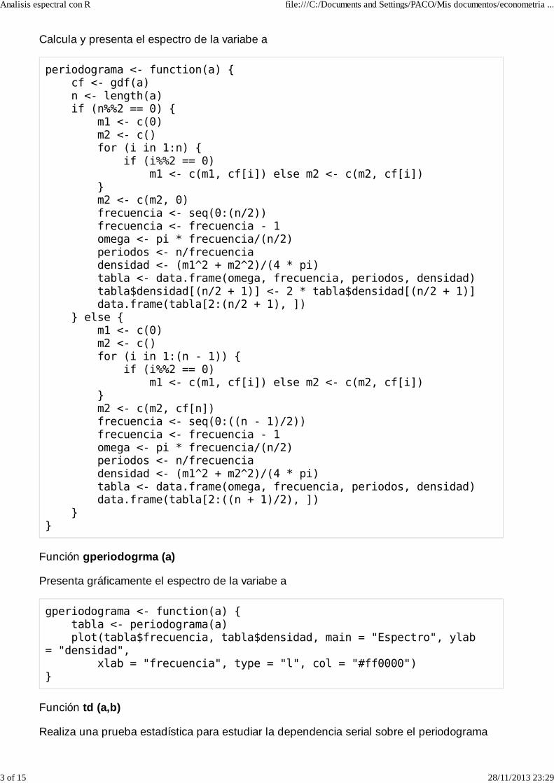
Calcula y presenta el espectro de la variabe a

periodograma <- function(a) { cf <- gdf(a) n <- length(a) if (n%%2 == 0) { m1 <- c(0) m2 <- c() for (i in 1:n) { if (i%%2 == 0) m1 <- c(m1, cf[i]) else m2 <- c(m2, cf[i]) } m2 <- c(m2, 0) frecuencia <- seq(0:(n/2)) frecuencia <- frecuencia - 1 omega <- pi * frecuencia/(n/2) periodos <- n/frecuencia densidad <- (m1^2 + m2^2)/(4 * pi) tabla <- data.frame(omega, frecuencia, periodos, densidad) tabla$densidad[(n/2 + 1)] <- 2 * tabla$densidad[(n/2 + 1)] data.frame(tabla[2:(n/2 + 1), ]) } else { m1 <- c(0) m2 <- c() for (i in 1:(n - 1)) { if (i%%2 == 0) m1 <- c(m1, cf[i]) else m2 <- c(m2, cf[i]) } m2 <- c(m2, cf[n]) frecuencia <- seq(0:((n - 1)/2)) frecuencia <- frecuencia - 1 omega <- pi * frecuencia/(n/2) periodos <- n/frecuencia densidad <- (m1^2 + m2^2)/(4 * pi) tabla <- data.frame(omega, frecuencia, periodos, densidad) data.frame(tabla[2:((n + 1)/2), ]) }}

Función gperiodogrma (a)

Presenta gráficamente el espectro de la variabe a

gperiodograma <- function(a) { tabla <- periodograma(a) plot(tabla$frecuencia, tabla$densidad, main = "Espectro", ylab = "densidad", xlab = "frecuencia", type = "l", col = "#ff0000")}

Función td (a,b)

Realiza una prueba estadística para estudiar la dependencia serial sobre el periodograma


3 of 15 28/11/2013 23:29

acumulado de a, con una significación de 0,1(b=1); 0,05(b=2); 0,025(b=3); 0,01(b=4) y 0,005(b=5) (Durbin; 1969)

td <- function(a, b) { per <- periodograma(a) p <- as.numeric(per$densidad) n <- length(p) s <- p[1] t <- 1:n for (i in 2:n) { s1 <- p[i] + s[(i - 1)] s <- c(s, s1) s2 <- s/s[n] } while (n > 50) n <- 50 if (b == 1) c <- Test[n, 1] else { if (b == 2) c <- Test[n, 2] else { if (b == 2) c <- Test[n, 3] else c <- Test[n, 4] } } min <- -c + (t/length(p)) max <- c + (t/length(p)) data.frame(s2, min, max)}

Fuction gtd (a,b)

Presenta graficamente los resultados de la prueba de Durbin (Durbin; 1969) :

gtd <- function(a, b) { S <- td(a, b) plot(ts(S), plot.type = "single", lty = 1:3)}

Función rbs (a)

Realiza la regresión band spectrum del vector de datos a con el vector de datos b para las dfrecuencias empezando por c.

rbs <- function(a, b, c, d) { a <- matrix(a, nrow = 1) n <- length(a) A <- c(1, rep(0, c - 1), rep(1, d), rep(0, n - c - d)) unos <- rep(1, n) lm1 <- lm(diag(A) %*% gdf(a) ~ 0 + diag(A) %*% gdf(b) + diag(A) %*% gdf(unos)) summary(lm1)}

Realiza la regresión dependiente del tiempo de los vectores a y b, en las d primeras


4 of 15 28/11/2013 23:29

frecuencias.

rdt <- function(a, b, d) { a <- matrix(a, nrow = 1) b <- matrix(b, nrow = 1) n <- length(a) f <- function(x) { for (i in 1:d) x[i] A <- c(x[1:d], rep(0, n - d)) B <- c(x[d + 1], rep(0, n - 1)) unos <- c(rep(1, n)) colSums((gdf(celec) - cdf(PIB) %*% t(t(A)) - cdf(unos) %*% t(t(B)))^2) } xmin <- optim(c(rep(1, d + 1)), f, NULL, method = "BFGS") A <- c(xmin$par[1:d], rep(0, n - d)) B <- c(xmin$par[d + 1], rep(0, n - 1)) fitted <- cdf(b) %*% t(t(A)) + cdf(unos) %*% t(t(B)) plot(b, a, pch = 19, col = "blue") lines(b, gdt(fitted), lwd = 3, col = "red") print(xmin) fitted <- gdt(fitted) betas <- gdt(A) alfha <- gdt(B) ta <- t(a) error <- ta - fitted ajuste <- 1 - colSums(error^2)/colSums(ta^2) print(fitted) print(betas) print(alfha) print(ajuste) plot(b, error, pch = 19, col = "blue") gtd(error, 2)}

Output:

Analisis PIB

periodograma(PIB)

## omega frecuencia periodos densidad## 2 0.3927 1 16.000 9.153e+09## 3 0.7854 2 8.000 2.266e+09## 4 1.1781 3 5.333 1.035e+09## 5 1.5708 4 4.000 6.284e+08## 6 1.9635 5 3.200 4.254e+08## 7 2.3562 6 2.667 3.206e+08## 8 2.7489 7 2.286 2.575e+08## 9 3.1416 8 2.000 2.406e+08

plot(ts(PIB), plot.type = "single", lty = 1:3)


5 of 15 28/11/2013 23:29

gperiodograma(PIB)

gtd(PIB, 3)


6 of 15 28/11/2013 23:29

## Error: object 'Test' not found

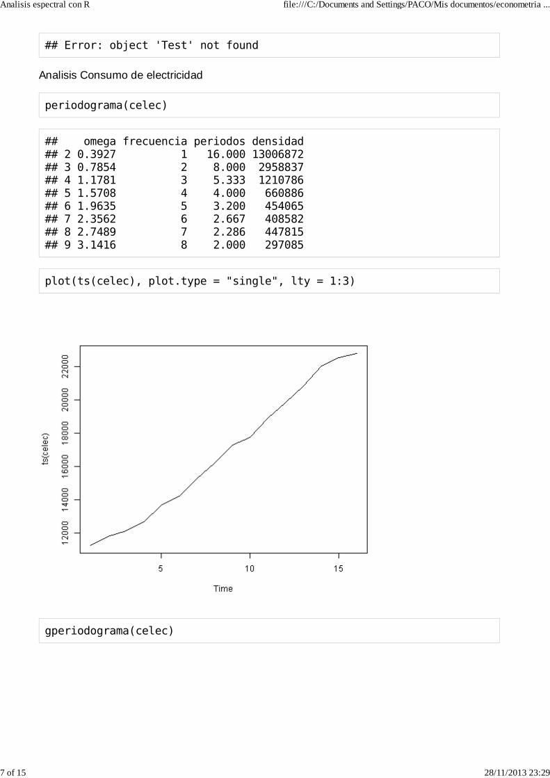
Analisis Consumo de electricidad

periodograma(celec)

## omega frecuencia periodos densidad## 2 0.3927 1 16.000 13006872## 3 0.7854 2 8.000 2958837## 4 1.1781 3 5.333 1210786## 5 1.5708 4 4.000 660886## 6 1.9635 5 3.200 454065## 7 2.3562 6 2.667 408582## 8 2.7489 7 2.286 447815## 9 3.1416 8 2.000 297085

plot(ts(celec), plot.type = "single", lty = 1:3)

gperiodograma(celec)


7 of 15 28/11/2013 23:29

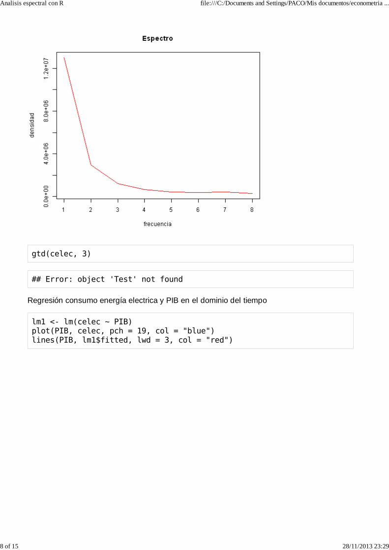
gtd(celec, 3)


Regresión consumo energía electrica y PIB en el dominio del tiempo

lm1 <- lm(celec ~ PIB)plot(PIB, celec, pch = 19, col = "blue")lines(PIB, lm1$fitted, lwd = 3, col = "red")


8 of 15 28/11/2013 23:29

summary(lm1)

## ## Call:## lm(formula = celec ~ PIB)## ## Residuals:## Min 1Q Median 3Q Max ## -334 -187 -111 213 378 ## ## Coefficients:## Estimate Std. Error t value Pr(>|t|) ## (Intercept) -6.65e+03 3.74e+02 -17.8 5.4e-11 ***## PIB 3.68e-02 5.79e-04 63.5 < 2e-16 ***## ---## Signif. codes: 0 '***' 0.001 '**' 0.01 '*' 0.05 '.' 0.1 ' ' 1## ## Residual standard error: 245 on 14 degrees of freedom## Multiple R-squared: 0.997, Adjusted R-squared: 0.996 ## F-statistic: 4.04e+03 on 1 and 14 DF, p-value: <2e-16

plot(lm1$residuals, celec, pch = 19, col = "blue")


9 of 15 28/11/2013 23:29

gperiodograma(lm1$residuals)

gtd(lm1$residuals, 3)


10 of 15 28/11/2013 23:29


Regresión consumo energía electrica y PIB en el dominio de la frecuencia

unos <- rep(1, 16)lm2 <- lm(gdf(celec) ~ 0 + gdf(PIB) + gdf(unos))summary(lm2)

## ## Call:## lm(formula = gdf(celec) ~ 0 + gdf(PIB) + gdf(unos))## ## Residuals:## Min 1Q Median 3Q Max ## -367.2 -29.7 115.6 214.2 370.5 ## ## Coefficients:## Estimate Std. Error t value Pr(>|t|) ## gdf(PIB) 3.68e-02 5.79e-04 63.5 < 2e-16 ***## gdf(unos) -6.65e+03 3.74e+02 -17.8 5.4e-11 ***## ---## Signif. codes: 0 '***' 0.001 '**' 0.01 '*' 0.05 '.' 0.1 ' ' 1## ## Residual standard error: 245 on 14 degrees of freedom## Multiple R-squared: 1, Adjusted R-squared: 1 ## F-statistic: 3.98e+04 on 2 and 14 DF, p-value: <2e-16

Regresión band spectrum del consumo de electricidad y el PIB para las 4/2 frecuencias,comenzando por la frecuencia de periodo n.

rbs(celec, PIB, 1, 4)


11 of 15 28/11/2013 23:29

## ## Call:## lm(formula = diag(A) %*% gdf(a) ~ 0 + diag(A) %*% gdf(b) + diag(A) %*% ## gdf(unos))## ## Residuals:## Min 1Q Median 3Q Max ## -216 0 0 0 403 ## ## Coefficients:## Estimate Std. Error t value Pr(>|t|) ## diag(A) %*% gdf(b) 3.74e-02 4.03e-04 92.6 < 2e-16 ***## diag(A) %*% gdf(unos) -7.01e+03 2.60e+02 -26.9 1.8e-13 ***## ---## Signif. codes: 0 '***' 0.001 '**' 0.01 '*' 0.05 '.' 0.1 ' ' 1## ## Residual standard error: 153 on 14 degrees of freedom## Multiple R-squared: 1, Adjusted R-squared: 1 ## F-statistic: 1.01e+05 on 2 and 14 DF, p-value: <2e-16

A <- c(rep(1, 5), rep(0, 11))unos <- rep(1, 16)lm5 <- lm(gdf(celec) ~ 0 + cdf(unos) %*% gdf(PIB) + gdf(unos))plot(PIB, celec, pch = 19, col = "blue")lines(PIB, gdt(lm5$fitted), lwd = 3, col = "red")

summary(lm5)


12 of 15 28/11/2013 23:29

## ## Call:## lm(formula = gdf(celec) ~ 0 + cdf(unos) %*% gdf(PIB) + gdf(unos))## ## Residuals:## Min 1Q Median 3Q Max ## -367.2 -29.7 115.6 214.2 370.5 ## ## Coefficients:## Estimate Std. Error t value Pr(>|t|) ## cdf(unos) %*% gdf(PIB) 3.68e-02 5.79e-04 63.5 < 2e-16 ***## gdf(unos) -6.65e+03 3.74e+02 -17.8 5.4e-11 ***## ---## Signif. codes: 0 '***' 0.001 '**' 0.01 '*' 0.05 '.' 0.1 ' ' 1## ## Residual standard error: 245 on 14 degrees of freedom## Multiple R-squared: 1, Adjusted R-squared: 1 ## F-statistic: 3.98e+04 on 2 and 14 DF, p-value: <2e-16

Realiza la regresión dependiente del tiempo de los vectores a y b, en la frecuencia de periodon y n/2.

rdt(celec, PIB, 5)


13 of 15 28/11/2013 23:29

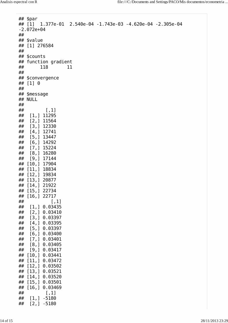
## $par## [1] 1.377e-01 2.540e-04 -1.743e-03 -4.620e-04 -2.305e-04 -2.072e+04## ## $value## [1] 276584## ## $counts## function gradient ## 118 11 ## ## $convergence## [1] 0## ## $message## NULL## ## [,1]## [1,] 11295## [2,] 11564## [3,] 12330## [4,] 12741## [5,] 13447## [6,] 14292## [7,] 15224## [8,] 16280## [9,] 17144## [10,] 17904## [11,] 18834## [12,] 19834## [13,] 20877## [14,] 21922## [15,] 22734## [16,] 22717## [,1]## [1,] 0.03435## [2,] 0.03410## [3,] 0.03397## [4,] 0.03395## [5,] 0.03397## [6,] 0.03400## [7,] 0.03401## [8,] 0.03405## [9,] 0.03417## [10,] 0.03441## [11,] 0.03472## [12,] 0.03502## [13,] 0.03521## [14,] 0.03520## [15,] 0.03501## [16,] 0.03469## [,1]## [1,] -5180## [2,] -5180


14 of 15 28/11/2013 23:29

## [3,] -5180## [4,] -5180## [5,] -5180## [6,] -5180## [7,] -5180## [8,] -5180## [9,] -5180## [10,] -5180## [11,] -5180## [12,] -5180## [13,] -5180## [14,] -5180## [15,] -5180## [16,] -5180## [1] 0.9999



15 of 15 28/11/2013 23:29